Download Simulated Human being a dissertation submitted in partial fulfilment

Simulated Human
being a dissertation submitted in partial fulfilment of
the requirements for the Degree of Master of Science
in the University of Hull
by
Vosinakis Spyridon
September 2000
Table of Contents
INTRODUCTION .....................................................................................................................................1
1.
ABSTRACT ......................................................................................................................................1
2.
STRUCTURE OF THE DISSERTATION ...............................................................................................1
BACKGROUND ........................................................................................................................................3
1.
INTRODUCTION ..............................................................................................................................3
2.
BODY MODELLING .........................................................................................................................4
3.
4.
2.1
Modelling the body...................................................................................................................4
2.2
Modelling the skeleton .............................................................................................................5
2.3
Modelling the skin and clothes.................................................................................................6
HUMAN ANIMATION ......................................................................................................................8
3.1
Body positioning: Forward and inverse kinematics................................................................8
3.2
Keyframing ...............................................................................................................................9
3.3
Motion Capture ......................................................................................................................10
3.4
Simulation...............................................................................................................................14
3.5
Hybrid Approaches ................................................................................................................17
APPLICATION FIELDS ...................................................................................................................18
PROJECT SPECIFICATION................................................................................................................20
1.
AIM OF THE PROJECT ....................................................................................................................20
2.
PROJECT STAGES..........................................................................................................................20
DESIGN ....................................................................................................................................................23
1.
INTRODUCTION ............................................................................................................................23
2.
CREATING AN ENVIRONMENT ......................................................................................................23
3.
MODELLING THE BODY................................................................................................................25
4.
BODY POSITIONING AND ANIMATION ..........................................................................................28
4.1
Joint rotations.........................................................................................................................28
4.2
Continuous skin ......................................................................................................................31
4.3
Keyframing .............................................................................................................................33
4.4
Walking animation .................................................................................................................34
5.
PHYSICALLY BASED MODELLING ................................................................................................35
6.
COLLISION DETECTION AND RESPONSE ......................................................................................37
6.1
Bounding Primitives...............................................................................................................38
6.2
Collision Detection.................................................................................................................40
6.3
Collision Response .................................................................................................................41
ii
7.
DYNAMIC BEHAVIOUR .................................................................................................................42
IMPLEMENTATION .............................................................................................................................45
1.
INTRODUCTION ............................................................................................................................45
2.
OPEN-GL .....................................................................................................................................45
3.
4.
2.1
Polygon Rendering .................................................................................................................46
2.2
Camera control.......................................................................................................................46
VISUAL C++ AND MFC ...............................................................................................................47
3.1
Mouse control.........................................................................................................................48
3.2
Keyboard, Menus and Dialogs...............................................................................................49
3.3
Timer.......................................................................................................................................50
POSER MODELS AND VRML IMPORT ..........................................................................................50
4.1
5.
The VRML file importer .........................................................................................................51
SKELETON DEFINITION AND MANIPULATION ..............................................................................54
5.1
The Joint Hierarchy files........................................................................................................55
5.2
Joint Matrices.........................................................................................................................56
6.
DESCRIPTION OF THE CLASSES ....................................................................................................57
7.
TESTING .......................................................................................................................................58
RESULTS .................................................................................................................................................60
1.
2.
DESCRIPTION AND USE OF THE PROGRAM ...................................................................................60
1.1
Camera control.......................................................................................................................60
1.2
Loading models and defining postures ..................................................................................61
1.3
Physically based modelling....................................................................................................62
1.4
Walking animation and other actions....................................................................................62
1.5
Demonstration ........................................................................................................................63
EXTENSIBILITY.............................................................................................................................64
CONCLUSIONS ......................................................................................................................................66
APPENDIX: USER MANUAL ..............................................................................................................68
1.
CD CONTENTS .............................................................................................................................68
2.
EXECUTING THE PROGRAM ..........................................................................................................69
3.
SUMMARY OF KEYS AND MENU COMMANDS ..............................................................................70
REFERENCES.........................................................................................................................................72
ADDITIONAL BIBLIOGRAPHY ........................................................................................................75
iii
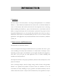
INTRODUCTION
1. ABSTRACT
The main subject of this dissertation is the design and implementation of a simulated
human, i.e. a three dimensional model that looks and acts like a real human. Besides the
review of the literature and the discussion about the most important issues concerning
human modelling and simulation, a project that demonstrates a virtual human with the
ability to navigate and interact with its environment is presented. The project has been
designed and implemented so as to be reusable and extensible, since its aim is not only to
demonstrate some features of a simulated human, but also to serve as a basis for future
applications. Such applications may include distributed virtual environments, simulation
systems, etc.
2. STRUCTURE OF THE DISSERTATION
The dissertation is structured as follows:
In the next chapter all the background and related work is presented. The focus is given
on the modelling of the body and the animation of a virtual human. Techniques such as
keyframing, motion capture and simulation are thoroughly described and compared to
each other. In the last part, the main application areas of human modelling and
simulation are briefly described.
The chapter that follows is the project specification, where the aims and objectives of the
project are analysed.
Next is the design chapter, where the design strategy and the theories and algorithms
behind it are explained and justified. It discusses about the definition of the 3D
environment, the body modelling, the pose generation and human animation, and the
collision detection between an object and the human body. The algorithms for major
1
problems such as physically based modelling, joint transformation, inverse kinematics,
collision detection and response are described in detail.
The chapter that follows discusses the implementation of the program and the
programming language and libraries that have been used. The use of OpenGL and
Microsoft Foundation Classes is explained, the algorithms are presented from the
programmer’s point of view and all the implementation techniques are explained.
Problems such as the import of the human mesh from a VRML file, the definition of
joint structure and posture information files, and the choice of data structures for the
body skin and skeleton are discussed. In the last part, the techniques employed for
testing the program are also described.
The implementation is followed by the results, a chapter that presents the final program
and its functionality. The various options and commands of the program are explained
and some screenshots are presented. The program is not only treated as a standalone
application, but also as a piece of code that can be extended and reused in future
applications. The second part of the chapter explores this side of the program.
In the last chapter of this dissertation are the conclusions. There is a comparison
between the aims and results of this project and a discussion about the difficulties of this
application area and the value of the project for graphics applications. The dissertation
closes with a description of possible future extensions.
After the conclusions there is an Appendix, which is the user manual, followed by the
References and the additional bibliography.
2
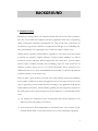
BACKGROUND
1. INTRODUCTION
Simulated (or virtual) humans are computer models that look and act like real humans.
They can vary in detail and complexity and can be applied in fields such as engineering,
virtual environments, education, entertainment, etc. They are also used as substitutes for
real humans in ergonomic evaluations of computer-based designs or for embedding realtime representations of live participants into virtual environments (Badler, 1999).
Human motion, interaction and simulation, especially for cases where an accurate model
is required, are extremely complex problems. Therefore human simulation is a field of
continuous research and many different approaches have taken place. Accurate human
motion requires complex physically based modelling, where the body should not be
treated as a passive object, but as a set of joints and muscles able to generate forces.
Additionally, there has to be an embedded behavioural model to help the body maintain
its balance and move in an effective way.
There has been a great amount of research in the field of human motion and simulation
and a number of different systems and approaches have been proposed. Each of them
varies in appearance, function and autonomy according to the application field and the
required detail and accuracy. Norman Badler, probably the most important researcher in
this field, proposes three separated stages for the development of a virtual human (Badler,
1993):
¾ body modelling: the visualisation of the overall human body and the definition of the
skeletal structure with proper joint motions.
¾ spatial interaction: the direct manipulation of the human joints or the creation of goaloriented motion based on constraints with the use of inverse kinematics algorithms.
3
¾ behavioural control: the ability to generate complex motion following a simple set of
rules that determine the model’s behaviour.
Obviously, these three stages differ in levels of complexity and each one is based on the
previous.
2. BODY MODELLING
The process of modelling a virtual human involves three different stages. The most
primitive one is the visualisation of the body, which is the same process as modelling any
other 3D object. This stage may be the only one required for producing static images, but
it is impossible to animate the body having only its 3D representation. Therefore, an
essential stage is the modelling of the skeleton, which will define the moving parts of the
body and the type of motion that they can perform. These two stages alone are enough
for simple, animated humans. Nevertheless, the production of natural-looking, believable
motion requires much more. Both the skin and the clothes of the virtual human should
move and deform in a natural way. The calculation of the skin and cloth motion is the
most computationally intensive task, which is why it is not suitable for real-time
animation.
2.1
Modelling the body
Modelling the human body follows the same process as modelling any other 3D object.
There are many ways to represent a figure geometrically (curved surfaces, voxels, etc),
but the most efficient one, especially for real-time applications, is to model the body as a
mesh (a set of vertices and polygons). The level of detail and complexity of the body
strictly depends on the application area. Games and real-time simulations tend to use
models with a small number of polygons and use alternative methods (e.g. textures) to
display detailed parts. On the other hand, in video or high quality image productions the
body is modelled with the maximum possible detail.
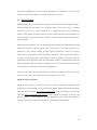
There are some commercial programs that allow users to define and construct a human
body model and export it in a 3D file format; probably the best known is Poser from
Metacreations (http://www.curiouslabs.com). With such programs, artists are able to select a
primitive model from a library, specify a number of visual details (such as height, muscle
4
size, face characteristics) and use this model in their own programs or animation
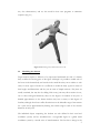
sequences (Fig. 2.1).
Figure 2.l: Human figure by Metacreations Poser ™
2.2
Modelling the skeleton
Proper motion requires a skeleton to be represented underneath the skin of a human
body to define the moving parts of the figure. Although it is possible to model each of
the bones in the human body and encode in the model how they move relative to each
other, for most types of motion it is sufficient to model the body segments in terms of
their lengths and dimensions and the joints in terms of simple rotations. The joints are
usually rotational, but may also be sliding. Each rotary joint may allow rotation in one,
two or three orthogonal directions; these are the degrees of freedom of the joint. A
detailed approximation to the human skeleton may have as many as 200 degrees of
freedom, although often fewer suffice. Restrictions on the allowable range of movements
for a joint can be approximated by limiting the rotation angle in each of the rotation
directions at each joint.
The individual objects comprising the skeleton are each defined in their own local
coordinate systems, and are assembled into a recognisable figure in a global world
coordinate system by a nested series of transformations. The fact that a change in the
5
rotation of one joint affects the position of several others makes it necessary to connect
them in a tree-structured topology (Badler, 1993). A change in the rotation of a node will
cause geometric transformations on all its leaf nodes.
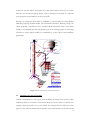
Recently, an attempt has been made to standardise a joint hierarchy for Virtual Reality
Modelling Language human models. The Humanoid Animation Working Group (HAnim) proposed a specification for a standard VRML humanoid (Roehl, 1999) which
includes a very detailed joint tree. The primary goal of the working group is to encourage
3D artists to create skeleton models in a standard way, so they can be used in different
applications.
Figure 2.2: The joint hierarchy proposed by H-Anim
2.3
Modelling the skin and clothes
Careful consideration has to be given when modelling the human skin, because, unlike
mechanical objects, movement of the human body causes the surface to deform. For
example, when the wheels of a car are turned, this rotation does not affect any other
parts of it, but when the human arm is rotated it causes a deformation of the skin around
6
the shoulder and chest. If the segments of the body are modelled as rigid objects, even
small rotations may cause unwanted ‘cracks’ on the skin and make the model look
unrealistic.
The simplest and easiest way to avoid this problem is to use fixed primitives in joints. These
primitives (usually spheres or ellipsoids) serve as a way to fill the cracks when the
segments are moving, giving the illusion of continuous skin. The visual results of this
technique are not as elegant as one might wish, but, due to its simplicity, it has been
adopted by many real-time systems, especially when less computational power is
available.
One other more efficient solution is deformation by manipulation of skin contours (Kalra,
1998). This technique does not treat body segments as static meshes, but deforms the
body’s geometry when a segment is rotated. The idea is to manipulate the cross-sectional
contours (set of points that lie on the same plane) of the body mesh. Every joint has to
be associated with a contour and it has to lie on the plane of this contour. When a
segment is rotated around a joint, the deformation of the skin around that joint is
determined by the two adjacent joints (the parent and the child in the joint hierarchy). If
the contour of the joint J1 that caused the rotation has normal N1 (the normal of the
plane on which the contour lies) and the two adjacent joints J0 and J2 have normals N0
and N2 respectively, the intermediate contours in the segments J0J1 and J1J2 are calculated
using linear interpolation between the normals. Once the normal of a contour is
calculated, all its vertices are transformed so as to lie on the new plane. This technique is
fast and efficient, but it cannot be applied to all body meshes. The body has to be
constructed using contours lying on planes perpendicular to the skeleton’s segments.
In cases where a high degree of realism is required, the skin’s motion has to follow the
laws of physics, it has to behave as an elastic surface. One way to achieve this is to model
the skin as a set of springs and masses (Vince, 1995). Each vertex of the surface mesh can
be treated as a small mass and each edge as a spring with a relatively high restitution
factor. This structure will ensure the elastic deformation of the skin while the body is
moving. It is nevertheless required that the surface mesh is as regular as possible and it
should be relatively dense as well.
There are also more complex approaches that use biomechanical models to determine
the skin’s behaviour and generate wrinkles while the skin is deforming (Wu, 1998,
7
Magnetat-Thalmann, 1996). These models additionally take the muscles of the body into
consideration and also calculate their deformation.
Cloth simulation follows almost the same process using a spring and mass model again.
The surface of the clothes has to be a dense set of small masses, which should have
gravity and be able to collide with themselves and the skin underneath. A more detailed
model (large set of springs and masses) will result in a more realistic deformation and
wrinkle generation of the clothes. Today’s computational power allows real-time cloth
animation using a simplified spring-mass model (Lander, 1999).
3. HUMAN ANIMATION
People are skilled at perceiving the subtle details of human motion. A person can, for
example, often recognise friends at a distance purely from their walk. Because of this
ability, people have high standards for animations that feature humans. For computergenerated motion to be realistic and compelling, the virtual actors must move with a
natural-looking style.
Specifying movement to a computer is surprisingly hard. Even a simple bouncing ball
can be difficult to animate convincingly, in part because people quickly pick out action
that is unnatural or implausible without necessarily knowing exactly what is wrong.
Animation of a human is especially time-consuming because numerous details of the
motion must be captured to convey personality and mood.
The techniques for computer animation fall into three basic categories: keyframing, motion
capture and simulation (Hodgins, 1998). All three involve a trade-off between the level of
control that the animator has over the fine details of the motion and the amount of work
that the computer does on its own. Keyframing allows fine control but it is the animator
who has to ensure the naturalness of the result. Motion capture and simulation generate
motion in a fairly automatic fashion but offer little opportunity for fine-tuning.
3.1
Body positioning: Forward and inverse kinematics
A body posture can be generated by varying the local rotations applied at each joint over
time, as well as the global translation applied at the joint root. There are two fundamental
approaches: the low-level forward kinematics approach and the more elegant inverse
kinematics one.
8
Forward kinematics involves explicitly setting the position and orientation of objects at
specific frame rimes. For skeletons, this means directly setting the rotations at selected
joints, and possibly the global translation applied to the root joint, to create a pose. Using
forward kinematics, the position of any object within a skeleton can only be indirectly
controlled by specifying rotations at the joints between the root and the object itself. In
contrast, inverse kinematics techniques provide direct control over the placement of an
end-effector object at the end of a kinematic chain of joints, providing a solution for the joint
rotations which place the object at the desired location (Welman, 1993).
Inverse kinematics, sometimes called ‘goal-directed motion’, offers an attractive alternative to
explicitly rotating individual joints within a skeleton. An animator can instead directly
specify the position of an end-effector, while the system automatically computes the joint
angles needed to place the part (Watt, 1992). The inverse kinematic problem has been
studied extensively in the robotics field, although it is only fairly recently that the
techniques have been adopted for computer animation.
In the case of forward kinematics the animator has more and more transformations to
control, which, while lending more freedom to achieve a more expressive animation, may
prove to be too complicated and intricate to achieve in practice. On the other hand,
inverse kinematics algorithms have a high computational cost, making it almost
impossible to calculate joint angles for all degrees of freedom of a virtual human in realtime. In most cases a balance between these two approaches is desired.
3.2
Keyframing
Borrowing its name from a traditional hand animation technique, keyframing requires
that the animator specify critical, or key, positions for the objects. The computer then
fills in the missing frames by smoothly interpolating between those positions.
The specification of keyframes can be partially automated with techniques that assist in
the placement of some body joints. If the hand of a character must be in a particular
location, for instance, the computer could calculate the appropriate elbow and shoulder
angles, using inverse kinematics. Although such techniques simplify the process,
keyframing requires that the animator has a detailed understanding of how moving
objects should behave over time as well as the talent to express that information through
9
keyframed configurations. The continued popularity of keyframing comes from the
degree of control that it allows over the fine details of the motion.
3.3
Motion Capture
Motion capture involves measuring an object's position and orientation in physical space,
then recording that information in a computer-usable form. Once data is recorded,
animators can use it to control elements in a computer-generated scene. Animation
which is based purely on motion capture uses the recorded positions and orientations of
the body parts to generate the paths taken by synthetic objects within the computergenerated scene.
Motion capture has proven to be an extremely useful technique for animating human and
human-like characters. Motion capture data retain many of the subtle elements of a
performer’s style, thereby making possible digital performances where the person’s
unique style is recognisable in the final product. Because the basic motion is specified in
real-time by the subject being captured, motion capture provides a powerful solution for
applications where animations with the characteristic qualities of human motion must be
generated quickly. Real-time capture techniques can be used to create immersive virtual
environments for training and entertainment applications.
There are three different techniques that can be used to record the motion of the body:
magnetic systems, optical systems and digital poseable mannequins (Dyer, 1995).
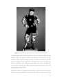
Magnetic Motion Capture
Magnetic motion capture systems use sensors to measure accurately the magnetic field
created by a source. Examples of magnetic motion capture systems include the Ascension
Bird and Flock of Birds (http://www.ascension-tech.com) and the Polhemus Fastrak and
Ultratrak (http://www.polhemus.com/home.htm) . Such systems are real-time, in that they can
provide from 15 to 120 samples per second (depending on the model and number of
sensors) of 6D data (position and orientation) with minimal transport delay.
10
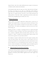
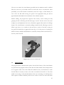
Figure 2.3: A performer in a typical configuration of magnetic motion capture sensors
A typical magnetic motion capture system has one or more electronic control units into
which the source and sensors are cabled. The electronic control units are, in turn,
attached to a host computer through a network or serial port connection. The motion
capture or animation software communicates with these devices via a driver program. The
sensors are attached to the scene elements being tracked. The source is set either above
or to the side of the active area. There can be no metal in the active area, since it can
interfere with the motion capture.
The obvious solution for magnetic motion capture is to place one sensor at each joint.
However, the physical limitations of the human body (the arms must connect to the
11
shoulder, etc.) allow an exact solution with significantly fewer sensors. Because a
magnetic system provides both position and orientation data, it is possible to infer joint
positions by knowing the limb lengths of the motion-capture subject.
Optical Motion Capture
Optical motion capture systems are based on high contrast video imaging of retro-reflective
markers which are attached to the object whose motion is being recorded. The markers
are small spheres covered in reflective material such as Scotch Brite.
The markers are imaged by high-speed digital cameras. The number of cameras used
depends on the type of motion capture. Facial motion capture usually uses one camera,
sometimes two. Full body motion capture may use four to six (or more) cameras to
provide full coverage of the active area. To enhance contrast, each camera is equipped
with infrared- (IR) emitting LEDs and IR (pass) filters are placed over the camera lens.
The cameras are attached to controller cards, typically in a PC chassis.
Depending on the system, either high-contrast (1 bit) video or the marker image
centroids are recorded on the PC host during motion capture. Before motion capture
begins, a calibration frame, ‘a carefully measured and constructed 3D array of markers’ is
recorded. This defines the frame of reference for the motion capture session.
After a motion capture session, the recorded motion data must be post-processed or
tracked. The centroids of the marker images (either computed then, or recalled from disk)
are matched in images from pairs of cameras, using a triangulation approach to compute
the marker positions in 3D space. Each marker's position from frame to frame is then
identified. Several problems can occur in the tracking process, including marker
swapping, missing or noisy data, and false reflections.
Tracking can be an interactive and time-consuming process, depending on the quality of
the captured data and the fidelity required. For straightforward data, tracking can take
anywhere from one to two minutes per captured second of data (at 120 Hz). For
complicated or noisy data, or when the tracked data is expected to be used as is, tracking
time can climb to 15 to 30 minutes per captured second, even with expert users. Firsttime users of tracking software can encounter even higher tracking times.
Digital Poseable Mannequins
12
The Digital Image Design Monkey (http://www.didi.com/www/areas/products/monkey2) is
the first commercial device to provide "motion capture" using poseable humanoid
figures or other morphological types. This class of devices should allow easier inclusion
of those familiar with the stop-motion work flow into computer animation. While these
devices may provide continuous data, it is not usually continuous motion that is being
captured but the position of the mannequin at discrete points in time.
The monkey consists of a poseable mannequin (typically sub-scale), position encoders
for each of the mannequin's joints, and an electronic control unit, which is attached to a
host computer. As the joints of the monkey are moved, the control unit tracks their
positions and passes them to a driver program on the host computer (this may either be
on request or by streaming). The joints on the monkey may be locked or tightened
individually, allowing adjustment of single joints. This implies a painstaking, though
familiar, workflow for the digital stop motion animator. Each frame, or keyframe, of an
animation sequence must be adjusted precisely then recorded using a motion capture
program.
Disadvantages of Motion Capture
Motion capture may have many advantages and commercial systems are improving
rapidly, but the technology has drawbacks. Both optical and magnetic systems suffer
from sensor noise and require careful calibration (O’Brien, 2000). Additionally,
measurements such as limb lengths or the offsets between the sensors and the joints are
often required. This information is usually gathered by measuring the subject in a
reference pose, but hand measurement is tedious and prone to error. Because of
constraints on mismatched geometry, quality constraints of motion capture data, and
creative requirements, animation rarely is purely motion capture based. In most of the
cases, animators have manually to alter the data to reach the desired results.
To maintain the integrity of motion-captured data, the scene elements being controlled
by the data should be as geometrically similar as possible. Depending on the degree that
the geometries are different, some compromises have to be made. Essentially, either
angles or positions can be preserved, though typically not both.
A simple example is that of reaching for a particular point in space. If the computerised
character is much shorter than the captured motion, the character must either reach up
13
higher to reach the same point in space (changing the joint angles), or reach to a lower
point (changing the position reached). As differences become more complicated, e.g. the
computer character is the same height as the human model but has shorter arms, so do
the compromises in quality.
Geometric dissimilarity and motion stitching are two of the most difficult problems
facing motion capture animators. Solutions to these problems, including inverse
kinematics and constrained forward kinematics, have had some success. However, these
techniques require substantial user intervention and do not solve all problems.
3.4
Simulation
Unlike keyframing and motion capture, simulation uses the laws of physics to generate
motion of figures and other objects. Virtual humans are usually represented as a
collection of rigid body parts. Although the models can be physically plausible, they are
nonetheless only an approximation of the human body. A collection of rigid body parts
ignores the movement of muscle mass relative to bone, and although the shoulder is
often modelled as a single joint with three degrees of freedom, the human clavicle and
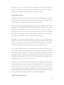
scapula allow more complex motions, such as shrugging. Recently researchers have
begun to build more complex models, and the resulting simulations will become
increasingly lifelike as researchers continue to add such detail (Hodgins, 1998, Kalra, 1998).
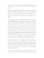
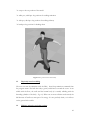
Figure 2.4: Simulated Human Running (© GeorgiaTech College of Computing)
When the models are of inanimate objects, such as clothing or water, the computer can
determine their movements by making them obey equations of motion derived from
14
physical laws. In the case of a ball rolling down a hill, the simulation could calculate
motion by taking into account gravity and forces such as friction that result from the
contact between the ball and the ground. But people have internal sources of energy and
are not merely passive or inanimate objects. Virtual humans, therefore, require a source
of muscle or motor commands--a "control system." This software computes and applies
torques at each joint of the simulated body to enable the character to perform the desired
action. A control system for jogging, for instance, must determine the torques necessary
to swing the leg forward before touchdown to prevent the runner from tripping (Hodgins,
1998).
Most control systems use state machines: algorithms implemented in software that
determine what each joint should be doing at every moment and then ensure that the
joints perform those functions at appropriate times (Hodgins, 1996). Running, for
example, is a cyclic activity that alternates between a stance phase, when one leg is
providing support, and a flight phase, when neither foot is on the ground. During the
stance phase, the ankle, knee and hip of the leg that is in contact with the ground must
provide support and balance. When that leg is in the air, however, the hip has a different
function--that of swinging the limb forward in preparation for the next touchdown. One
state machine selects among the various roles of the hip and chooses the right action for
the current phase of the running motion.
Associated with each phase are control laws that compute the desired angles for each of
the joints of the simulated human body. The control laws are equations that represent
how each body part should move to accomplish its intended function in each phase of
the motion. To move the joints into the desired positions, the control system computes
the appropriate torques with equations that act like springs, pulling the joints toward the
desired angles. In essence, the equations are virtual muscles that move the various body
parts into the right positions.
In recent years, researchers have worked on simulation-based methods that generate
motion without requiring the construction of a handcrafted control system. Several
investigators have treated the synthesis of movement as a trajectory optimisation
problem (Witkin, 1988, Gleicher, 1997). This formulation treats the equations of motion
and significant features of the desired action as constraints and finds the motion that
expends the least amount of energy while satisfying those restrictions. To simulate
jumping, the constraints might state that the character should begin and end on the
15
ground and be in the air in the middle of the motion. The optimisation software would
then automatically determine that the character must bend its knees before jumping to
get the maximum height for the minimum expenditure of energy. Another approach
finds the best control system by automatically searching among all the possibilities. In the
most general case, this technique must determine how a character could move from
every possible state to every other state. Because this method solves a more general
problem than that of finding a single optimum trajectory from a certain starting point to
a particular goal, it has been most successful in simple simulations and for problems that
have many solutions, thereby increasing the probability that the computer will find one.
Fully automatic techniques are preferable to those requiring manual design, but
researchers have not yet developed automatic methods that can generate behaviours for
systems as complex as humans without significant prior knowledge of the movement.
Other researchers have tried to add emotions to simulated human motion. (Unuma,
1995). Fourier expansions of experimental data of actual human behaviours serve as a
basis from which this method can interpolate or extrapolate the human locomotion. This
means, for instance, that transition from a walk to a run is smoothly and realistically
performed by the method. For example, the method gets ‘briskness’ from the
experimental data for a ‘normal’ walk and a ‘brisk’ walk. Then, the ‘brisk’ run is generated
by the method using another Fourier expansion of the measured data of running. The
superposition of these human behaviours is shown as an efficient technique for
generating rich variations of human locomotions. In addition, step – length, speed, and
hip position during the locomotions are also modelled, and then interactively controlled
to get a desired animation.
Advantages and Disadvantages
As a technique for synthesising human motion, simulation has two potential advantages
over keyframing and motion capture. First, simulations can easily be used to produce
slightly different sequences while maintaining physical realism -for example, a person
running at four meters per second instead of five. Merely speeding up or slowing down
the playback of another type of animation can spoil the naturalness of the motion.
Second, real-time simulations allow interactivity, an important feature for virtual
environments and video games in which artificial characters must respond to the actions
of an actual person. In contrast, applications based on keyframing and motion capture
select and modify motions from a precomputed library of movements.
16
Although control systems are difficult to construct, they are relatively easy to use. An
animator can execute a simulation to generate motion without possessing a detailed
understanding of the behaviour or of the underlying equations. Simulation enables
control over the general action but not the subtle details. For instance, the animator can
dictate the path for a bicycle but cannot easily specify that the cyclist should be riding
with a cheerful, light-hearted style. This limitation could be overcome in part by using
simulation to generate the gross movements automatically and then relying on
keyframing or on motion capture for the finer motions, such as facial expressions.
One drawback of simulation, is the expertise and time required to handcraft the
appropriate control systems. Another disadvantage is the computational cost. Virtual
environments with dynamically simulated actors need multiple processors with either
virtual or physical shared memory to obtain the required performance (Brogan, 1998).
Dynamic simulation also imposes some limitations on the behaviour of synthetic
characters. Simulated characters are less manoeuvrable than those modelled as pointmass systems and those that move along paths specified by animators. For example,
although a point-mass model can change direction instantaneously, a legged system can
change direction only with a foot planted on the ground. If the desired direction of travel
changes abruptly, the legged system may lose its balance and fall. These limitations,
although physically realistic and therefore intuitive to the user, make it more difficult to
design robust algorithms for group behaviours, obstacle avoidance, and path following.
3.5
Hybrid Approaches
Besides Keyframing, Motion Capture and Simulation there are also approaches that use a
combination of these. In most of the cases motion captured data are combined with
simulation algorithms to retain the important characteristics of dynamic simulation while
extracting the stylistic details found in human motion data. Z. Popovic and A. Witkin
propose an algorithm for transforming character animation sequences that preserves
essential physical properties of the motion (Popovic, 1999). The algorithm constructs a
simplified character model and fits the motion of the simplified model to the captured
motion data. From this fitted motion it obtains a physical spacetime optimisation
solution that includes the body’s mass properties, pose, footprint constraints and
muscles. From this altered parameterisation it computes a transformed motion sequence.
The motion change of the simplified model is mapped back onto the original motion to
produce a final animation sequence. This algorithm is well suited for the reuse of highly
17
detailed captured motion animations. A similar approach (Zordan, 1999) is using
simulation to animate models with different dynamic and kinematic parameters from
motion captured data.
4. APPLICATION FIELDS
Virtual humans can be useful in many different application areas, especially in cases
where human activity has to be visualised. Depending on the application, a virtual human
can have different roles as:
¾ an actor: all its actions are predefined by a script or other means. The main application
field is video / film production.
¾ an agent: it acts as an autonomous entity and its actions depend on the environment.
Agents are usually found in simulations and virtual environments.
¾ an avatar: it serves as a visual representation of an actual person, so its actions are
guided (in real-time) by that person. The main application fields are virtual
environments and video games.
The most important application fields that use or will use the current research on virtual
humans are (Badler, 1997):
¾ Engineering, Design and Maintenance: Analysis and simulation for virtual prototyping and
simulation­based design. Design for access, ease of repair, safety, tool clearance,
visibility, and hazard avoidance.
¾ Virtual Environments / Virtual­Conferencing: Efficient tele­conferencing using virtual
representations of participants to reduce transmission bandwidth requirements.
Living and working in a virtual place for visualization, analysis, training, or just the
experience.
¾ Education / Training: Skill development, team coordination, and decision­making.
Distance mentoring, interactive assistance, and personalized instruction.
¾ Games and Entertainment: Real­time characters with actions and personality for fun and
profit.
18
Besides general industry­driven improvements in the underlying computer and graphical
display technologies themselves, virtual humans will cause significant improvements in
applications requiring personal and live participation.
In building models of virtual humans, there are varying notions of virtual fidelity.
Understandably, these are application dependent. For example, fidelity to human size,
capabilities, and joint and strength limits are essential to some applications such as design
evaluation. On the other hand in games, training, and military simulations, temporal
fidelity (real­time behaviour) is essential (Badler, 1999).
Probably the most important application that utilises many aspects of human motion and
simulation is a commercial system called Jack, developed at the University of
Pennsylvania (Badler, 1998). It contains kinematic and dynamic models of humans based
on biomechanical data. Furthermore, it allows the interactive positioning of the body and
has several built-in behaviours including balance, reaching and grasping, walking and
running. The Jack model contains almost all the essential human skeletal joints and it can
be scaled to different body sizes based on population data.
19
PROJECT SPECIFICATION
1. AIM OF THE PROJECT
There may be a considerable amount and variety of research going on in the field of
human modelling and simulation, but not all the aspects of the problem have yet been
explored. Applications like Jack mainly focus on the accuracy of the simulation and have
far too many details on human body structure, because their main target is the field of
industrial design (and similar fields that need detailed results). Therefore, such systems
run only in powerful workstations. On the other hand, applications such as Virtual
Environments are not based on accuracy. They require natural looking motion as well as
acceptable execution speed and this is the aspect that this project will focus on. The aim
of this project is the design and implementation of a virtual human, a human model that
is able to execute actions and interact with its environment in near real-time.
The results of this project can be extended in many ways. First of all, it can be used for
photorealistic video production (since all the motion data can be extracted), where the
animation will look much more realistic compared to the traditional approach of
manually entering the motion sequence. Then, a real-time simulated human can be also
inserted in Virtual Environments (such as 3D conference rooms, virtual classrooms, etc.)
as synthetic actor and increase the believability of the virtual world. Additionally,
complex simulations which involve human action (e.g. fire emergency in a building) can
take advantage of the results of this project.
2. PROJECT STAGES
The project will be based on the C++ programming language and the OpenGL graphics
library. Microsoft Foundation Classes will be used for the windowing interface. A
physically based modelling (PBM) component will be created to simulate the physics of
the human body and the environment. The human model will be imported from a
20
commercial 3D-modelling package (such as Metacreations Poser or Animation Master)
and a hierarchy tree will be designed to support the animation of the human body parts.
The next step will be to apply coordinated transformations in the human parts and
generate complex and, if possible, goal-oriented animation sequences, such as walking or
grasping an object. Finally, a simple simulation environment containing one or more
instances of the virtual human will be set-up. Focus will be given on the functionality and
extensibility of the implemented code to allow this project to be a basis for future work.
The stages of the project will be:
¾ Implementation of a simple 3D environment: An MFC application that will be the basis of
the project’s implemented system. The environment will be able to load 3D polygons
from a file and display them using OpenGL. The implemented file format will
support material (diffuse colour, specular colour and shininess) for each polygon and
transformations (translation, rotation, scale and centre of rotation) for sets of
polygons. Furthermore, the user will be able to change the position and orientation
of the viewpoint to visualise different aspects of the 3D world.
¾ Physically based modelling: A component able to simulate physical forces and apply them
to the world’s objects causing a change in one or more of their attributes (position,
orientation etc.). The simulation will be executed in discrete time steps using the
Euler method of numerical integration and besides physical forces (such as friction,
collision and gravity) it will also take into account those generated by the human
muscles.
¾ Definition of a joint hierarchy: The human body will be divided into joints and segments
and a geometric transformation tree will be designed. Each body part will have
certain degrees of freedom and specified limits in its movement. The level of detail
and complexity of the defined hierarchy will be carefully chosen, since it will affect
the accuracy, the amount of computation needed to generate proper motion and the
overall performance. A good approach will be to allow more than one level of detail
and to be able to switch between them. Some joints will simply remain static (will
have fixed attributes) if the detail level has been decreased.
¾ Import of human model: A primitive human model will be imported from a 3D
modelling package and used as the basic model of the project. The vertices and faces
21
of the 3D object will be converted to the implemented file format and the defined
joint hierarchy will be applied to it. Again, the graphic detail of the human model will
be such that it does not affect too much the overall performance.
¾ Definition and testing of primitive motion: The independent rotation of different body
segments is regarded as primitive motion. A dialog will allow the user to change the
attributes and create different postures of the human model. Then, the system will be
tested on the accuracy and naturalness of the motion and, if necessary, the joint
hierarchy and the human model will be adapted.
¾ Definition of complex motion (multiple joints): The first task will be to define series of
simultaneous transformations to different body parts and generate complex
animations. Then, the physically based modelling component will be applied and the
body muscles will be able to generate forces. A number of different combinations
will be tested to achieve certain tasks. The first objective will be to apply forces in
such a way that the body balance is maintained and then, if possible, more complex
tasks involving motion will be tried.
¾ Set up of a simple simulation: The final aim will be to use the previous results in a simple
application: a simulation environment that will involve one or more virtual humans.
The nature of the simulation will depend on the achieved complexity in the previous
steps.
22
DESIGN
1. INTRODUCTION
The design stage of this project has been a very important phase, because of the
problem’s complexity and the number of design decisions that had to be taken. The most
basic part of the project has been the definition and modelling of a 3D environment. The
next stage was modelling of the body and skeleton of the virtual human, followed by the
positioning of the body and animation stages. After that, physically based modelling and
collision detection had to be defined, while the virtual human had to demonstrate some
dynamic behaviour as well.
2. CREATING AN ENVIRONMENT
The graphical environment is the basis of this project. It is the context in which a virtual
human ‘exists’, the means to visualise its appearance and actions. This effort aims to
display graphics that are realistic enough to be used in virtual environments or other realtime simulations, therefore the use of a three dimensional environment is essential.
There are a number of different approaches to generating three dimensional objects, but
currently the most efficient one for real-time applications is the use of 3D Polygons. This is
mainly because they are supported by all hardware accelerated graphics cards, making the
rendering of a scene a very fast process with relatively good quality. Additionally, creating
polygonal objects is straightforward and visually effective algorithms exist to produce
shaded versions of objects represented in this way. All other approaches have to make
use of the CPU to visualise the virtual space, thus increasing the rendering time
dramatically and making it almost impossible to render complex scenes in real time.
In the polygonal approach, each three-dimensional object is represented by a mesh of
polygonal facets. In the general case, an object possesses curved surfaces and the facets
are an approximation to such a surface. Polygons may contain an arbitrary vertex number
or be restricted to triangles. It may be necessary to do the latter to gain optimal
23
performance from special-purpose hardware or graphics accelerator cards. In the
simplest case, a polygon mesh is a structure that consists of polygons represented by a list of
linked (x, y, z) coordinates that are the polygon vertices. Thus, the information stored to
describe an object is finally a list of points or vertices.
In all solid objects, adjacent polygons share common vertices; therefore it is a waste of
memory to store the same vertices two, three or more times in a mesh structure. At first
this waste may seem insignificant, but one should not forget that with current technology
some graphics scenes can have hundreds of thousands of polygons. A more efficient
approach is to have a list of all vertices stored in the mesh structure and have the
polygons point to the vertices.
Some objects of the scene may contain curved surface parts and it is important for them
to be rendered smoothly to add realism to the images. This is necessary for applications
containing virtual humans because the human body itself is full of curved parts. Shading
algorithms use the normal vector at the vertex of each polygon to create a smooth shading
effect on a curved surface. Therefore a normal vector should be assigned to each vertex
and stored together in the mesh structure.
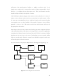
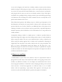
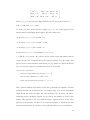
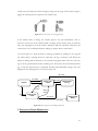
The scene structure of this project is depicted in the following class diagram (Fig. 4.1).
Scene
*
Light
Camera
1
*
Mesh
*
Polygon
1
Material
2
Vector
3..*
*
Point
Figure 4.1: The class diagram of the scene elements
24
As seen in the diagram, each mesh has an arbitrary number of points and an arbitrary
number of polygons. Each polygon can point to three or more points and each point has
two vectors, the vertex and the normal. Besides these, a material (colour) is associated to
each polygon and the scene can also have an arbitrary number of lights. Each light is
considered to be a pointlight having a unique position in space and emitting equal energy
in all directions. The final image that will be rendered from the scene depends on the
position and orientation of the camera.
Three dimensional geometry and shading can give a relatively good perception of the
third dimension. Nevertheless, the exact position of objects in the virtual space is better
perceived with the use of shadows. Therefore, one additional feature of this project is the
rendering of shadows cast by the objects onto the ground. This is especially important in
animation sequences, where the distance of the virtual human’s feet to the ground can be
visually estimated.
Conceptually, drawing a shadow is a simple process. A shadow is produced when an
object blocks light from a light source from striking another object or surface behind the
object casting the shadow. The area on the shadowed object’s surface, outlined by the
object casting the shadow, appears dark. A shadow can be produced by flattening the
original object into the plane of the surface, which in this case is the ground plane. The
idea is to create a transformation matrix that flattens any 3D object into a twodimensional polygon. No matter how the object is oriented, it is squashed into the plane
in which the shadow lies. This matrix depends on the position of the light source and the
coefficients that determine the plane.
3. MODELLING THE BODY
A virtual human is a part of the scene, therefore it has to be represented in terms of
polygons like any other object. The human body could be one big polygon mesh, but it
would be very difficult to animate it. If, for example, the virtual human had to raise its
arm, the program would have to find which vertices and polygons belong to the arm and
rotate only these. A much better approach is to define the body as a set of smaller
meshes, each one representing a segment (limb). Each segment is the body part that
connects two joints and should maintain its geometry throughout the animation.
25
The number of joints and segments that will be defined on the human body depends on
the application and the animation detail required. So does the number of degrees of
freedom allowed per joint. A real human has in total over two hundred degrees of
freedom, but efficient animation can be produced with significantly less. A simple
walking animation may need less than a dozen joints. On the other hand, a virtual human
that can grasp various objects requires a lot of additional joints and segments (for the
fingers of each hand). In this project a virtual human can have an arbitrary number of
joints and segments and any possible hierarchy tree to connect them. This gives the user
/ programmer the ability to load any possible models and adjust the program to the
needs of different applications having any possible detail.
The human body representation is something that should also be arbitrary. Therefore,
the program does not work with a fixed model, but is able to load models dynamically.
The model should follow a file format and be a set of polygon meshes as described in the
previous paragraph. Additionally, each mesh should have a unique name. The process of
loading a human body model is as follows:
for each mesh
read the set of vertices
read the set of normals and assign them to the vertices
for each polygon
find the corresponding vertices and assign pointers to them
read the set of colours and assign them to the polygons
Although the human body is now ‘split’ into a set of independent polygon meshes, they
themselves are not enough to animate it. The skeletal information is necessary to define
how these meshes are going to be transformed. This is loaded from a supplementary file,
which has the following data:
¾ the joint hierarchy: The tree structure that connects the joints. With this structure one
can identify the joints and segments that are going to be affected if a joint is rotated.
For example a raise in the arm affects the position of the wrist and the hand. As
stated before, all meshes have a unique name, which is also the name of the segment
they represent. To avoid introducing new names for the joints, each joint has the
name of the segment that it directly affects. For example the name of the wrist joint
is ‘hand’.
26
¾ the joint position: The joints have a maximum of three degrees of freedom; they allow
only rotations. Therefore, each joint has a fixed position that is also the centre of
rotation for all its descendants in the tree structure.
¾ the joint limits: A real human cannot rotate his/her limbs arbitrarily in all directions;
every joint has certain limits. These limits are introduced in the virtual human’s joints
as six numbers: the minimum and the maximum rotation angle per degree of
freedom.
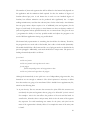
The joint hierarchy tree that is being used in the default models of the project is shown
in the Figure 4.2.
Hip
Left Thigh
Abdomen
Right Thigh
Left Shin
Chest
Right Shin
Left Foot
Left Collar
Neck
Right Collar
Left Shoulder
Head
Right Shoulder
Left Forearm
Right Forearm
Left Hand
Right Hand
Right Foot
Figure 4.2: A sample joint tree
As stated before, the skeletal information is a tree structure. Each node of the tree
(which is actually a joint) is stored in a class called TreeNode. This class has the following
properties:
¾ the position of the joint
¾ the three rotation angles of the joint
¾ a pointer to the mesh that it directly affects
¾ an array of pointers to the descendant nodes
27
The assignment of a mesh to a TreeNode should be done in the beginning of the
program by comparing the name property of a mesh with the joint name. The head of
the hierarchy tree (which is usually the Hip node) defines the global translation and
rotation of the body and can, of course, access the whole set of joints of the virtual
human. In the general case, where one application uses more than one virtual human,
there should be a Person class with a pointer to the head of the hierarchy tree. The
Person class should also have the entire set of meshes that define the body of the virtual
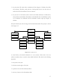
human. The class diagram for these classes is the following (Fig. 4.3).
Person
1
Treenode
*
1
*
Mesh
Figure 4.3: The class diagram of the Person, Mesh and Treenode classes
4. BODY POSITIONING AND ANIMATION
4.1
Joint rotations
When the human model is loaded all joint angles are zero. The posture of the model is its
initial pose and every other transformation is applied on this pose. This means that every
posture is actually a set of rotations on the initial pose. Although nothing prevents a
model from having any arbitrary pose as the initial one, the same pose will look entirely
different on two different models if their initial one is not the same. Therefore, it is
necessary that all models start from the same pose if the predefined animation is going to
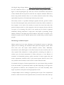
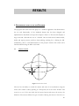
be applied to them. The most common initial pose among the programs/protocols that
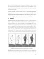
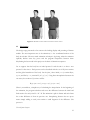
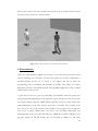
animate virtual humans and the one used in this program is the following (Fig. 4.4).
28
Figure 4.4: A sample initial position for virtual human.
Each pose is a set of rotations applied on joints. For example a raise in the arm is one
rotation applied on the shoulder joint. There are two ways to define a rotation: using a
rotation axis and one angle, or using three angles, one per axis. The second approach has
been adopted, mainly due to its simplicity in both defining a rotation and manipulating it.
Each of the three rotation angles is compared to the joint limits (the maximum and
minimum angle value per axis) and the program determines if it is valid or not.
Let us suppose that the joint Ji has a rotation Ri (rxi, ryy, rzi) and a position Pi [ pxi, pyi, pzi
]. The joint rotates the segment Si and all its descendants in the hierarchy tree. The
vertices of Si are defined in absolute coordinates (world coordinates) and not in terms of
the joint centre Pi. This means that they cannot be directly rotated by Ri, because after
the rotation Si will not be attached to Ji anymore. The rotation should be around Pi,
which is the joint centre and thus the centre of rotation for Si and all its descendant
nodes.
The process of rotating a mesh is actually the multiplication of its vectors by a matrix.
Both vertices and normal vectors should be multiplied by a special 3×3 matrix, the
rotation matrix.
The following matrix rotates points about an arbitrary axis passing
through the origin:
29
⎡ ka x2 + c
⎢
⎢ka x a y + sa z
⎢ ka x a z − sa y
⎣
ka x a y − sa z
ka y2 + c
ka y a z + sa x
ka x a z + sa y ⎤
⎥
ka y a z − sa x ⎥ ,
ka z2 + c ⎥⎦
where [ ax, ay, az ] is the unit vector aligned with the axis; θ is the angle of rotation; c =
cosθ, s = sinθ, and k = ( 1 – cosθ ).
To rotate one point around the three angles (rx, ry, rz), one should generate three
rotation matrices and multiply them together. The three matrices are:
¾ Rx with [ ax, ay, az ] = [ 1 0 0 ] and θ = rx,
¾ Ry with [ ax, ay, az ] = [ 0 1 0 ] and θ = ry and
¾ Rz with [ ax, ay, az ] = [ 0 0 1 ] and θ = rz.
For all vertices v = [ vx vy vz ] and normals n = [ nx ny nz ]:
v′ = (RxRyRz)v = R v and n′ = R n, where v′ and n′ are the vertices and normals after the
rotation and R is the 3×3 matrix that results from the product of Rx, Ry, and Rz. This
process rotates a mesh around the world centre [ 0 0 0 ], which is not always the desired
case. To rotate the segment Si around the joint centre Pi one should:
For each vertex v and normal n
subtract the centre of rotation from the vertices: v′ = v – Pi
rotate the vertices and normals: v′′ = Rv′, n′ = Rn
add the centre of rotation to the new vertices: v′′′ = v′′ + Pi
This is still not sufficient. The rotation of the joint Ji should also be applied to all other
segments that follow in the hierarchy tree. For example, in fig. 4.2, a rotation in the Right
Thigh should also affect the Right Shin and the Right Foot. Therefore, the abovementioned process should be repeated for the vertices and normals of several other
meshes. This approach is not very efficient, because segments that are in the lower
positions of the hierarchy tree have to be rotated several times to determine the final
vertex and normal values for a posture. A more efficient solution is to use 4×4 matrices.
30
A 4×4 matrix can both rotate and translate a vector when multiplied with it. The general
form of a transformation matrix is:
⎡ r11
⎢r
⎢ 12
⎢ r13
⎢
⎣0
r21
r22
r31
r32
r23
0
r33
0
tx ⎤
⎡ r11
t y ⎥⎥
, where ⎢⎢r12
tz ⎥
⎥
⎣⎢ r13
1⎦
r21
r22
r23
r31 ⎤
r32 ⎥⎥ a rotation matrix R and [ tx ty tz ] a
r33 ⎦⎥
translation vector T. The question that arises is how to multiply a 4×4 matrix with 3dimensional vectors. The idea is to add a fourth dimension to the vectors, which will also
determine their type. So, instead of using [ x y z ] vertices will be in the form of [ x y z 1 ]
and normals [ x y z 0 ]. If one multiplies the transformation matrix with any four
dimensional vector, one will find out that if the fourth value is one the vector will be
both translated and rotated; in the case of zero it will only be rotated. Therefore, it is very
practical to use 4×4 matrices and 4D vectors, because the program does not need to
determine if a vector is vertex or normal. They will all be multiplied by the same matrix.
Each time a segment has to be rotated, its vertices and normals will be multiplied by a
4×4 matrix. This single matrix will be the product of all the transformations that should
have been applied to the segment. For example, if the segment Si has to be rotated by the
joint Ji, its normals and vertices will be multiplied by the matrix M, where:
⎡1
⎢0
M= ⎢
⎢0
⎢
⎣0
0 0 − pxi ⎤
⎡1
⎥
⎢0
1 0 − py i ⎥
RxRyRz ⎢
⎢0
0 1 − pz i ⎥
⎥
⎢
0 0
1 ⎦
⎣0
0 0
1 0
0 1
0 0
px i ⎤
py i ⎥⎥
pz i ⎥
⎥
1 ⎦
For each joint Ji one can find the corresponding local transformation matrix Mi which
should be applied to the descending segments. Each segment’s final coordinates depend
on the transformations from all previous joints. The final transformation is determined
by a single 4×4 matrix, which is the product of all corresponding matrices of the previous
joints in the hierarchy tree. For example, in the hierarchy of fig. 4.2, the final
transformation matrix of the Right Foot mesh will be M = M′M′′M′′′, if M′, M′′ and M′′′
are the local transformation matrices of the Hip, the Right Thigh and the Right Shin
respectively.
4.2
Continuous skin
31
Let us suppose that the segments Si and Sk are connected through the joint Jk. If Jk is
rotated, Sk will be rotated, but Si will not. This will cause a crack around the joint, as
already described in the Background chapter. There are many ways to deal with this
problem and the simplest one is to have fixed primitives (usually spheres) on the joints.
The major drawback of this approach is the fact that these primitives do not always fit
perfectly with the model’s meshes, thus distorting the appearance of the model. Another
problem is that these spheres add a lot more polygons to the scene and decrease the
performance significantly.
In this project a different approach has been adopted. Instead of having primitives at the
joints, the idea is to have the ends of adjacent segments always connected with each
other. The human model, in its initial pose, has a continuous skin. This means that
adjacent meshes share common vertices and each one uses its own copy. If the program
can ensure that whenever a segment is rotated the vertices that are common with any
adjacent segment will not be rotated, then no crack is going to appear. The effect of this
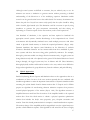
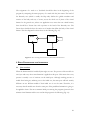
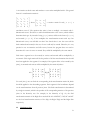
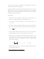
method can be seen in fig. 4.5.
Sj
Si
Sj
Si
crack
common
vertices
Figure 4.5: Segment rotation without and with common vertices
In the beginning of the program, when the model is loaded, each mesh checks its
adjacent ones if they share common vertices, i.e. if there are vertices with the same value.
Let us suppose that the mesh of the segment Si and that of Sj share the vertices v1, v2, …
vn. Each of the common vertices that belongs to Sj is being deleted and replaced with a
pointer to the corresponding vertex of Si. This means that all the polygons of Sj that
contain one or more of the common vertices will be projected using the values of the
corresponding vertices of Si. These vertices, that donot belong to Sj are marked as such
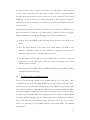
and are not rotated when Sj is being rotated (fig. 4.5). The visual result is that all the
polygons of Sj that are connected with Si (due to the common vertices) are stretched or
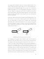
squeezed when the mesh is rotated, having the effect of a continuous skin (fig. 4.6).
32
Figure 4.6: Shoulder rotation without and with common vertices
4.3
Keyframing
The design stage presented so far concerns the loading, display and posturing of human
models. The next important state is the animation, i.e. the coordinated motion of the
body in real-time. The most usual animation technique is keyframing, where the animator
explicitly defines some key poses and the program interpolates between them.
Keyframing has been used in this project as the basis of animation sequences.
Let us suppose that the body has an initial posture P1 and the aim is to have a new
posture P2 after time t1. Each posture can be described with the set of all joint rotations
and the global translation of the body. Let the joint Ji have initial (t = 0) rotation R(rxi,
ryi, rzi) and final (t = t1) rotation R′ (rxi′, ryi′, rzi′). Using linear interpolation between the
two states, the rotation of Ji at time t will be
Rt( (t1-t)rxi + trxi′, (t1-t)ryi + tryi′, (t1-t)rzi + trzi′)
There is, nevertheless, a simpler way of calculating the interpolation. In the beginning of
the animation, the program calculates and stores the difference between the initial and
final rotation for each joint: D = R′ - R. The animation is split in frames and each frame
has a time difference dt from its previous one. Interpolating between the two poses
means simply adding to each joint rotation a small fragment of the difference. The
process is:
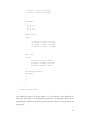
For each frame k repeat
33
For each joint i
Ri = Ri + dtD
until k*dt = t1
This generates a smooth transition between two states (poses). The use of this basic
process is made clear in the following example, the walking animation.
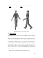
4.4
Walking animation
The animation of a walking human is a typical keyframing example. This is because of
the nature of walking, which is a continuous transition between several states. The aim of
walking is not only to continuously change the joint rotations, but also the global
translation of the body, causing the human to move towards a certain target. Walking has
the following states:
¾ State 1: the left leg touches the ground and pushes the body forward
¾ State 2: the right leg is on the ground and drives the body
Nevertheless, a walking animation should contain two more states. One is the transition
from current position to state 1 to start walking, and the other is the transition from any
state to a rest position to stop walking.
During each state the virtual human is also changing its global translation to animate the
body motion. This change should always follow the walking direction, which can be
determined directly from the global rotation of the body. In the initial position the
human body is facing the screen, so its direction vector is [ 0 0 1 ]. During any walking
process, the direction vector d is the rotation of the initial vector [ 0 0 1 ] by the global
rotation angles. If the virtual human is walking on a flat field the rotation around the yaxis will determine its direction.
The state – transition process presented so far is only capable of animating walking along
a straight line. However, in most of the cases, the virtual human may have to change its
direction while walking. This can not be done simply by interpolating the global rotation,
because the motion will not look natural. In reality, humans use their feet to rotate; they
can’t just turn their bodies while walking. The body rotation is a motion that has two
states, as shown in fig. 4.7. These two states may not be enough, because one cannot
34
usually rotate the body more than 90 degrees using just two steps. If the rotation angle is
bigger the rotation process is split into two smaller ones.
Figure 4.7: The two states for rotating the body
If the human body is resting, the rotation process can start immediately. This is,
however, not the case if the virtual human is walking. If the rotation starts on arbitrary
time, one leg might be in the air and the animation will look unnatural. Therefore, the
rotation has to be coordinated with the walking to achieve better visual results.
As seen in figure 4.7, when the body is rotating, the human is standing on one leg and
the whole body is rotating around it. After that, the leg is rotated as well. When the
human is walking and the body has to be rotated, the program waits until one of the two
legs is on the ground and the body is standing on it. The body is then rotated around that
leg, so that the whole process is animated smoothly and realistically enough. The state
diagram for the walking process is shown in figure 4.8
Stop rotating
Start walking
Stationary
Stop walking
Left Leg on the
Ground
Start rotating
Rotation around
Left Leg
Left Leg
forward
Right Leg
forward
Stop walking
Right Leg on the
Ground
Rotation around
Right Leg
Stop rotating
Start rotating
Figure 4.8: State diagram for the walking animation
5. PHYSICALLY BASED MODELLING
35
Traditional animators rely upon a mixture of visual memory and drawing skills to
simulate various physical behaviours. When a line test reveals that the animator is not
correct, it is redrawn and re-tested until it satisfies the animator. Unfortunately, such
techniques cannot be used in real-time computer graphics. If the aim is realism, one must
rely upon deterministic procedures that encode knowledge of the physical world. These
procedures are either based upon empirical laws or try to mimic a particular physical
behaviour.
Simulations that are based on moving objects usually rely upon Newton’s laws of
motion. Although they focus on the primary behaviours of theoretical particles having
mass but no size, they can however be employed to describe the motion of very large
objects without introducing significant errors.
Newton’s first law of motion states that ‘the momentum of a particle is constant when there are no
external forces’. In other words, an object moves in a straight line unless disturbed by some
force. In reality, the universe is full of gravitational, electric, magnetic or atomic force
fields and in general it is only when objects move away from the earth that they begin to
obey this law.
Newton’s second law of motion states that ‘a particle of mass m, subjected to a force F moves
with acceleration F/m’. This law is also called the equation of motion of a particle, and
means that work has to be done whenever an object is accelerated.
Newton’s third law of motion states that ‘if a particle exerts a force on a second particle, the
second particle exerts an equal reactive force in the opposite direction’. This law is useful when
considering collisions between objects.
One cannot just code Newton’s laws in a computer program and expect to have a perfect
simulation. There is a great difference between the theory and the implementation in
computer programs; in theory the time is considered to be continuous, while computers
work with discrete timesteps. The numerical integration used in computer programs
causes inevitable errors, usually in the form of energy discrepancy. A general rule is that
the error can be minimised with the use of smaller timesteps and better integration
methods, but these have computational costs. The primary aim of real-time simulations,
including this project, is not to be 100% accurate, but to achieve a good balance between
execution speed and realism. Therefore, in most of these cases the Euler Integration
36
method is being used, which is the simplest form of integration, but can still have
realistic results if the timestep is small enough.
The physical simulation is conducted in discrete timesteps. Each object has its own mass,
position and velocity and in each timestep its position and velocity are recalculated
following the laws of kinematics and collision. In this project the system executes the
following commands in each timestep dt:
For each object
1. Calculate the total force F applied to it. This will give rise to acceleration a such
that: F = m ⋅ a . From this equation the system can find the value of a.
2. If the velocity in the previous timestep was v0, then the current velocity v is:
v = v 0 + a ⋅ dt .
3. If the object’s position in the previous timestep was p0, its new position p will be the
result of the mean velocity between the previous and the current timestep. So:
p = p0 +
v + v0
⋅ dt .
2
4. Check if the object collides with any other object in the scene. If not, assign the new
position p and the new velocity v to the object and proceed to the next one.
5. Assuming that the other object did not move during dt find the position pc of the
object exactly when the collision occurred. Find the relation λ between the impact
position and the current one to approximate the exact time of impact and the
object’s velocity at that time.
λ=
pc − p0
p − p0
,0<λ≤1
vc = λ ⋅ v
dt c = λ ⋅ dt
6. Assign the position pc and velocity vc to the object and repeat the process (go to step
1) for the rest of the time dt - dtc.
6. COLLISION DETECTION AND RESPONSE
37
In a simulated environment all objects have to behave as rigid bodies, i.e. no object
should be allowed to penetrate another. The process of collision detection is to examine
if the whole or part of the geometry of an object is within another. Associated with this is
another equally important process, that of collision response, which should determine
the new position and velocity of the two (or more) objects that collided.
Calculating an accurate collision detection and response for a human body mesh is not
an easy task. One has to check each polygon of the mesh against all the other objects of
the scene and determine if it is penetrating another polygon. This is a very slow process,
especially for scenes containing virtual humans, where the total number of polygons will
be some thousands. There are of course acceleration techniques that can be used to
prevent testing collision against all other polygons, like the use of bounding boxes, but
polygon – polygon collision detection is still a very inefficient process for real-time
systems.
6.1
Bounding Primitives
There are a number of other collision detection techniques that are more efficient than
polygon – polygon collision detection but, as expected, less accurate. Nevertheless, the
primary aim of real-time systems is not accuracy. It is true that the more accurate the
calculations are the more believable the visual results will be, but efficiency is still the
most important issue. One interesting technique is to compare bounding geometrical
primitives of groups of polygons instead of comparing the polygons themselves. The
most used primitives are spheres and boxes mainly due to their simplicity, which makes
penetration tests much easier.
Having one giant bounding box or sphere around the entire human body mesh is far
from being a good solution to the collision detection problem. If an object were near the
human body it would collide with an “invisible” box or sphere. A much better approach
is to have one bounding primitive per body limb. The use of bounding spheres is still not
a good solution, because a sphere is equally large in all dimensions, which is not the case
in most of the human limbs. Only the head and hands would fit quite well in a bounding
sphere.
The bounding box is a much better approach since all the limbs fit very well inside
boxes, but there is one important drawback; the collision response. The box has the
38
problem that it contains corners, edges and flat parts, which will make the response of
colliding objects look very strange. For example, if an object (e.g. a ball) collides with the
human arm, its response will not be predictable, because it might hit a side of the
bounding box, an edge or a corner. The reflected velocity (after the collision) will be a
matter of luck. This situation can be avoided if one uses primitives with a certain degree
of symmetry, such as ellipsoids. Ellipsoids donot have corners and edges and they are
symmetrical around one axis. They have, nevertheless, other limitations. Mathematically
they are much more complex primitives compared to spheres and boxes making the
collision detection much harder to compute in real time. One good compromise between
all the previous geometric primitives is the cylinder (Fig. 4.9). It is fairly symmetrical, body
limbs fit well in it, and it is not very complex to calculate collision detection with it.
Therefore, this solution has been adopted for the collision detection of the human body
with its environment.
The bounding cylinders need to be calculated once and then they are only translated and
rotated following the motion of the limbs they correspond to. This calculation can be
done initially, when the human model is loaded. The process is simple and follows the
next three stages for each limb (mesh) of the body:
1. Calculation of the bounding box. One has to check all vertices of the mesh and find the
highest and lowest x, y and z values. The result will be two vectors (low and high)
which will define the corners of the bounding box. The size and centre of the box
can be found very easily: size = high – low and centre = high + low .
2
2. Cylinder type. Each cylinder can be aligned on the x, y or z axis. The use of arbitrary
cylinders has been avoided because it would complicate the calculations significantly.
This is not a drawback, since they can be rotated and translated as any other object in
the scene; it just affects their initial definition. The axis on which the cylinder will be
aligned will be the one with the highest value in the size vector of the bounding box.
3. Centre, radius and height. The cylinder’s centre is the centre of the bounding box. Its
height (or length, or width, depending on the axis) is the size value of the axis on
which it is aligned. The cylinder’s diameter is the mean between the size values of the
two other axes. For example, if the cylinder is aligned on the x-axis and the size
39
vector of the bounding box is [ sx sy sz ], then the length will be sx and the diameter
sy + sz
. So the radius is going to be sy + sz .
2
4
Figure 4.9: A human mesh covered by bounding cylinders
6.2
Collision Detection
After defining the initial position and size of each cylinder the next step is to check for
collision with other objects in the scene. In each timestep the cylinders have the
translation and rotation of the limbs they correspond to, so the collision detection has to
be done with the transformed cylinders and not with the initial ones. Although this
should complicate the calculations, there is a trick that can avoid this complication. Let
us, for example, check if a transformed cylinder collides with a sphere. Instead of
transforming the cylinder one could inverse transform the position and velocity of the
sphere and check for collision with the initial cylinder. If the objects collided, the new
position and velocity of the sphere has to be transformed back to the original coordinate
system. The steps are:
1. Find the matrix of the corresponding mesh and calculate its inverse.
40
2. Multiply the inverse matrix with the centre and velocity of the sphere
3. Check if the sphere collides with the initial cylinder
4. If they do, calculate the new position and velocity values and multiply them with the
transformation matrix.
The collision detection of a primitive with a cylinder is not a very complex task. Let us
consider the case of an x-aligned (horizontal) cylinder and test if a point is inside it. Let
the centre of the cylinder be [ cx cy cz ], its radius be R and its length l. Let also the point
be [ px py pz ]. The point is inside if and only if:
¾ cx -
l
l
≤ px ≤ cx +
and
2
2
¾ the distance of the point from the cylinder’s axis is less than the radius. In other
words:
(cy − px )2 (cz − pz )2
≤ R.
Similarly one can check if an edge is penetrating a cylinder, and with these two primitives
(points and edges) one can test boxes, polygons or any kind of mesh.
6.3
Collision Response
If a collision with the cylinder has been detected, the next step is to determine the
collision response, i.e. the new position and velocity of the object that has collided with
it. The general rule is that the velocity of the object after impact is equal to the reflection
of the velocity before impact if the collision is perfectly elastic and there is no friction
(Fig. 4.10). The reflection of the object’s velocity can be found with the use of the
normal vector of the cylinder’s surface point with which the object has collided. If the
unit normal at the point of collision is N and the velocity on impact is vI, the velocity vr
after impact will be: v r = v i − 2(v i ⋅ N ) ⋅ N . There are two cases:
1. The object has collided with one of the two disks of the cylinder. The normal vector is the
vector of the plane on which the disk lies. In the previous example the normal is
either [ 1 0 0 ] or [ -1 0 0 ] depending on the disk.
2. The object has collided with the cylinder’s body. The normal is the vector that results from
the difference between the point of collision and its projection on the cylinder axis.
41
In the previous example, if [ px py pz ] is the point of collision, the normal is the unit
vector of [ 0 (py-cy) (pz-cz) ].
vr
vi
N
Figure 4.10: The reflected velocity after the collision
7. DYNAMIC BEHAVIOUR
The term Dynamic Behaviour refers to actions executed by a virtual human that are not
predefined, but adapted to an ever-changing environment. This is, therefore, a very
important issue for simulation systems, because, in most of the cases, their objects /
creatures have to act in a dynamic environment. Virtual humans with embedded dynamic
behaviour demonstrate the most primitive form of ‘intelligence’, i.e. the ability to decide
on their actions according to the state of the environment. Besides simulation, this can
also be an important feature of virtual environments. Dynamic Behaviour could lead to a
higher level of control and a more ‘intelligent’ response of avatars as well as a more
believable, human-like behaviour of virtual agents.
In this project, the physically based modelling part inevitably ‘generates’ a dynamic
environment (where objects obey gravity), and the virtual human has to possess dynamic
behaviour to interact with the environment. The most primitive dynamic action is to
follow a moving object, e.g. a ball. This action can be implemented by using the most
basic principle of intelligent agents, the look – decide – act scheme.
Obviously the ‘look’ part is to read the coordinates (position in space) of the ball. A
more sophisticated version of it would be to be able to look at the ball only if it is within
the virtual human’s field of view, but one might argue that the virtual human could also
get a hint for the ball’s position by the sound that it makes when it bumps to the floor.
The ‘decide’ part is to choose if the virtual human should continue walking forward or
rotate its body. This decision is based on comparing the position of the ball with the
42
virtual human’s walking direction. The last phase is the action itself, where the body will
walk one step forward or rotate towards the ball.
More complicated dynamic actions involve catching a moving object or hitting it. These
actions must use a form of inverse kinematics, because they involve more than one joint
that have to be coordinated to succeed. Instead of using a generic inverse kinematics
solver, a different approach is introduced. This approach tests at every step the best
rotation for each joint to achieve the target.
The set of joints (or the joint chain) that are going to be used by the system are first
defined. Then, a function has to be assigned and return on how close to the target is the
current state of the virtual human is. The process is:
For each join in the chain
For each degree of freedom of the joint
increase and decrease angle by a value v
check which of the two states improves the function
if that state is different from the previous one decrease the value of v.
or else increase it (if lower than the maximum speed)
assign the value to the angle
This process is repeated in each frame and the system always corrects itself towards the
target. The speed of rotation change per joint depends on the success of the move. If
one segment is ‘shaking’ (the angle is increased in one step and decreased in the next, or
vice versa), the joint speed is decreased to provide finer approach to the target. On the
other hand, if an angle change is always heading towards the correct direction, the speed
is increased until it reaches the maximum value.
This procedural algorithm tries to mimic the real human behaviour. In reality, we do not
know the exact target state of our arm when we try to reach for an object. Starting from
an initial state, we continuously correct ourselves until we fulfil our target. Additionally,
this algorithm is less complex than the common inverse kinematics solvers and can even
work for moving targets. It also takes the joint limits into account to avoid unnatural
poses.
43
One example of using the above-mentioned algorithm is to have the virtual human reach
for a ball. In the case of fig. 4.2 the joint chain would be: Abdomen (to allow the body to
bend), Left Shoulder, Left Forearm. The target function would return the distance
between the Left Arm and the ball.
44
IMPLEMENTATION
1. INTRODUCTION
This chapter discusses some implementation issues of the project. It describes the use of
OpenGL and Visual C++ for the scene rendering and the interface, analyses the way the
VRML parser works and imports the virtual human geometry from files, and describes
the use and structure of the joint hierarchy files. The program’s classes and the testing
methods that have been employed are also described.
2. OPEN-GL
OpenGL is a library of graphics routines available on a wide variety of hardware
platforms and operating systems, including Windows 95, Windows NT, OS/2, Digital’s
Open VMS, and X Windows. It was developed by Silicon Graphics Incorporated in the
year 1992, and was eventually accepted as an industrial standard for hardcore 3D
graphics. The OpenGL Architecture Review Board maintains the library ensuring that
OpenGL is implemented properly on various platforms. This makes porting the
programs across the platforms much easier. OpenGL routines are well structured, highly
stable, intuitive, scalable from PCs to Super Computers and guaranteed to produce
consistent visual displays across various platforms.
OpenGL is defined as ‘a software interface to graphics hardware’. In essence, it is a 3D
graphics and modelling library that is extremely portable and very fast. OpenGL is not a
programming language, like C or C++. It is more like the C runtime library, which
provides some pre-packaged functionality. There really is no such thing as an “OpenGL
program”, but rather a program the developer wrote that uses OpenGL as one of its
APIs.
There has been extensive use of the OpenGL graphics library in this project. The camera
control and rendering of the 3D scene is based on OpenGL commands, which ensure
both quality and efficiency of the visual output. The reason for choosing OpenGL
45
instead of any other 3D graphics library is because OpenGL takes full advantage of the
hardware acceleration of current graphics cards and is therefore much more efficient that
any other ‘software-only’ approach. The only other API, which also uses graphics
accelerators, is Microsoft’s Direct 3D. The major drawback in using Direct 3D is that
compared to OpenGL it is a much more ‘low-level’ library and one needs more time and
effort to create graphics applications. Additionally, Direct 3D code can only work in
PC’s, so one cannot create platform-independent code and have his/her applications
running in powerful workstations.
2.1
Polygon Rendering
OpenGL does not only support triangles; it can render any polygons. This proved to be
very important, because the imported models were not triangle-based, so no additional
triangulation method was needed. A sample OpenGL code to display a polygon on
screen is the following:
glColor3f(r, g, b); // assign colour
glBegin(GL_POLYGON);
for(i=0; i<n; i++) { // for each edge
glNormal3f(normal[i].x, normal[i].y, normal[i].z); //normal
glVertex3f(vertex[i].x, vertex[i].y, vertex[i].z); //vertex
}
glEnd();
This code displays a polygon with n edges and colour (r, g, b), where its normals and
vertices are stored in normal[ ] and vertex[ ] arrays. The rendering of the scene in the
project was actually the process of scanning all the mesh objects of the scene, and for
each mesh displaying all its polygons using the previous piece of code. The only
additional code was the definition of the lights (position, direction and intensity) and the
viewing transformation that defined the distance and angle of the camera.
2.2
Camera control
OpenGL renders the scene from a fixed viewpoint and direction, so the only way to
define a camera transformation is to inverse transform the world. For example, if the
camera is at the point P and has a viewing angle (θx, θy, θz), in OpenGL one will have to
translate the world by –P and then rotate it by (-θx, -θy, -θz). This can be expressed in
OpenGL code as follows:
46
glPushMatrix();
glRotatef(-θx, 1.0, 0.0, 0.0); //rotation around x-axis
glRotatef(-θy, 0.0, 1.0, 0.0); //rotation around y-axis
glRotatef(-θz, 0.0, 0.0, 1.0); //rotation around z-axis
glTranslatef(-px, -py, -pz); //translation
render(); // a function that renders the world
glPopMatrix();
One other way of defining the camera is to have its focus fixed on a certain point P of
the world and rotate it around that point. This is very practical in cases like examining an
object (where the fixed point should be the object’s centre). In such cases the world first
has to be rotated around the point –P and then translated to the desired distance of the
camera D. The appropriate OpenGL code would be:
glPushMatrix();
glTranslatef(0.0, 0.0, -dist);
glRotatef(-θx, 1.0, 0.0, 0.0); //rotation around x-axis
glRotatef(-θy, 0.0, 1.0, 0.0); //rotation around y-axis
glRotatef(-θz, 0.0, 0.0, 1.0); //rotation around z-axis
glTranslatef(-px, -py, -pz); //translation
render(); // a function that renders the world
glPopMatrix();
The program has four different camera states that can be selected from the menu and
uses both camera models to implement them.
3. VISUAL C++ AND MFC
The project has been programmed in C++. There are two reasons for choosing C++ as
an implementation language. First of all, the program had to be written in an objectoriented language, because its aim is not only to be a standalone application, but also to
have an easily extensible and reusable code. Therefore, languages like C or Pascal (which
does not have full object support) are not suitable. On the other hand, the focus of this
project is real-time display capabilities; therefore the program had to be as efficient as
possible. Java might be a good object-oriented language, but it is not as efficient as C++
(because it uses an interpreter) and it does not have OpenGL support. As a conclusion,
the most efficient object-oriented approach was C++.
C++ alone is not enough to create graphical applications with OpenGL. The
programmer also needs a windows interface that will enable the application to run in
Microsoft Windows. This project is using the Microsoft Foundation Class (MFC) Library
47
Application Framework as a C++ interface to the Windows API. MFC, which is fully
supported by Microsoft Visual C++, is both efficient and relatively easy to use. Some of
the features of MFC which indicate why it is a very important tool for windows-based
applications are:
¾ Full support for File Open, Save and Save As menu items and the most recently used
file list
¾ Print preview and printer support
¾ Full support for the common controls in the released version of Windows95
¾ Classes for thread synchronisation
The use of MFC in this project resulted in a rich application interface. The use of
keyboard and mouse input, menus and dialogs gives the user the ability to have a better
control of the program. The mouse is used to control the camera, the keyboard to move
the virtual human and select different actions and the menus to use the various options
of the program (e.g. file import / export) and switch between different states (e.g. camera
types).
3.1
Mouse control
The mouse input has been handled with three different functions:
¾ OnLButtonDown( ): this function is called once, when the user presses the left mouse
button
¾ OnLButtonUp( ): this function is called once, when the user releases the left mouse
button
¾ OnRButtonDown( ): this function is called once, when the user presses the right mouse
button
¾ OnRButtonUp( ): this function is called once, when the user releases the right mouse
button
¾ OnMouseMove( ): this function is called when the user is moving the mouse.
48
The mouse is used in the project to rotate the camera and zoom in or out. The rotation is
achieved while the user is holding the left mouse button and moves the mouse. If the
mouse is moved to the left or right (x-axis) the world is rotated around the y-axis. A
move up or down (y-axis) rotates the world around the x-axis. Respectively, zooming in
or out requires the user to hold the right button and move the mouse. To achieve this
effect, the following technique has been used:
¾ There is a variable which can have three states: ROT if the world is being rotated,
ZOOM if the camera zooms in or out and NOOP if none of the above happens.
¾ In the OnLButtonDown( ) function ROT state is activated
¾ In the OnRButtonDown( ) function ZOOM state is activated
¾ In the OnLButtonUp( ) and OnRButtonUp( ) functions NOOP state is activated.
¾ In the OnMouseMove( ) function the system checks which is the current state. If it is
NOOP, it saves the mouse position and exits. If it is ZOOM, it checks the distance
between current mouse position and the previous one and zooms in or out in
proportion to the y-distance between the two mouse positions. If it is ROT it rotates
the world around the y-axis proportionally to the x-distance between the two mouse
positions and around the x-axis proportionally to the y-distance.
3.2
Keyboard, Menus and Dialogs
Keyboard handling follows the same idea. There are two functions, OnKeyDown( ) and
OnKeyUp( ) that are called when the user presses or releases a key respectively. There
are keys that activate actions of the virtual human and need to be pressed once. These
are handled directly in the OnKeyDown( ) function. On the other hand, the cursor keys
have a different role. They make the virtual human walk as long as they are pressed.
These keys indicate that the walking process started in the OnKeyDown( ) function and
that it stopped in the OnKeyUp( ) one. When the program updates the screen, it checks
if the walking state is enabled or not and calls the appropriate method.
The menu commands are simpler to control, since MFC provides a function for each
menu command that can be called by the user. The program also uses one dialog (fig.
5.1), which allows the user to select a body part of the virtual human and rotate it. The
49
dialog contains a combo box that has all the available limbs, and when the user presses
OK, it marks the pointer of the object that he/she has selected.
Figure 5.1: The dialog to select body part
3.3
Timer
The application uses a global timer to generate the animation sequences. There is a timer
function, provided by the MFC, which is called at a constant timestep. The length of this
timestep defines the frame rate of the application. Nevertheless, slower computers may
have fewer frames per second due to the inability of the hardware to render the scene in
a time smaller than or equal to the timestep. A frame rate greater than 30 frames/sec is
acceptable for animation, but really smooth motion is achieved in rates over 60
frames/sec.
The timer function updates the position and orientation of the scene elements (including
the camera) and redraws the scene. In this way, the scene is refreshed at constant rates.
The timer’s actions in a timestep are:
¾ update the ball’s position (due to gravity and collisions).
¾ update the virtual human’s global position and the orientation of joints if walking is
enabled
¾ update some joint rotations if a concurrent action is enabled
¾ redraw the scene
4. POSER MODELS AND VRML IMPORT
50
As stated in the design chapter, the program should import the 3D geometry of virtual
humans from files. The implemented version supports VRML models created by
Metacreations Poser. Poser is an application especially built for generating and rendering
human models, therefore it is very suitable source for 3D geometry files of humans. It
can export the human meshes in various file formats, such as .3ds (3D Studio), .dxf
(Autocad), and .wrl (VRML 97). The latter has been chosen, because VRML is fully
documented and it has an ASCII file format, which, although more difficult to parse,
makes the testing and debugging of the file importer easier.
4.1
The VRML file importer
The program is able to import any VRML file exported by Poser. Nevertheless, it does
not have a generic VRML parser, since this is outside of the scope of this project. It
exploits the way Poser generates the .wrl files and can parse only these files.
The Virtual Reality Modelling Language is a file format for the description of 3D virtual
worlds. It was initially built to display 3D worlds over the Internet and was only
supported by a few VRML plug-ins. Nowadays almost all 3D modelling and rendering
applications support it and it has become one of the most common 3D file formats. It is
in ASCII form.
The most basic element of VRML is the Node. A .wrl file is actually a set of nodes and
links between them. Nodes have different types (geometry, lighting, camera,
transformation, etc) and each node has a set of attributes. The values of the attributes
can be numbers, arrays or other Nodes. The most common and basic Node of VRML is
Shape, which describes the geometry of an object. The geometry could be either a simple
primitive (such as sphere, box, cylinder, etc) or a mesh. The Node that stands for a mesh
is called IndexedFaceSet and is the one that has to be parsed from the .wrl file. A sample
Shape node in a file exported by Poser is the following:
DEF Left_Thigh Shape
{
appearance Appearance { material Material { } }
geometry IndexedFaceSet
{
coord Coordinate
{
point
[
0.0024036 0.309619 -0.0272996
0.0023017 0.320267 -0.0277575
51
0.0208637 0.328671 -0.0431539
0.0359573 0.316325 -0.0483461
…
]
}
coordIndex
[
0 1 2 3 -1
3 2 4 -1
5 6 7 8 -1
9 5 8 10 -1
…
]
normal Normal
{
vector
[
-0.879089 -0.013376 -0.47647
-0.0736596 -0.871212 -0.48535
-0.0792951 -0.44513 -0.891948
-0.262508 -0.0100572 -0.964877
…
]
}
color Color
{
color
[
0.470573 0.337255 0.239216
0.117647 0.0784314 0.0352941
0.105882 0.0666667 0.0313726
0.454902 0.188235 0.160784
…
]
}
colorPerVertex FALSE
colorIndex
[
0
0
1
2
…
]
}
}
# DEF Left_Thigh Shape
The VRML files exported by Poser contain a set of such Shapes, which define all the
body parts. Each shape has an IndexedFaceSet geometry. The important attributes in the
IndexedFaceSet definition that define the mesh geometry and have to be parsed by the
program are:
52
¾ the point array in the Coordinate node: it contains all the vertices of the mesh. Every three
numbers is an (x, y, z) set of a new vertex.
¾ the coordIndex array: it defines the polygons of the mesh. Each polygon is a set of
numbers terminated by –1. Each of these numbers is an index to a vertex in the
point[ ] array. The indices start from zero, e.g. 0 1 2 –1 defines a triangle that
connects the first, second and third vertex of the point[ ] array.
¾ the vector array in the Normal node: it has the normal vectors of the mesh. The normal
vectors are not assigned to the polygons, but to the vertices for smooth display. The
nth vector in the vector[ ] array is the normal vector of the nth vertex in the point[ ]
array.
¾ the color array in the Color node: it has all the colours that are used in the mesh (each
polygon can have a different colour). The colours are in RGB format ranging from
0.0 to 1.0 for each of the red, green and blue values.
¾ the colorIndex array: it has the indices of the colours for each polygon. For example, if
the nth number in the colorIndex[ ] array is 1, it means that the nth polygon of the
mesh should have the second colour from the color[ ] array.
The VRML parser locates all Shape nodes in the file and for each one of them it reads all
the previously-stated arrays and stores the values in memory.
point array
The program continuously reads strings from the file using the standard C++ streaming
operators until it locates the ‘point’ keyword. It reads another string (the ‘[‘ character) and
then starts reading vectors until a ‘]’ character is read. The number of points in a mesh is
not pre-defined, therefore the use of a static array is not suitable, because it would have
great memory consumption. On the other hand, the use of double linked lists would
slow down the execution of the program (since tracking the nth element of a list needs at
least n steps). The way to get around this was to use a dynamic list for intermediate storage
and then, when the reading is over and the number of vertices is known, to allocate
memory for the point array (fig. 4.1) and copy the vertices from the list to the array. This
approach is both efficient and not memory consuming.
53
coordIndex array
The program locates the ‘coordIndex’ keyword. It reads another string (the ‘[‘ character)
and then starts reading polygons until a ‘]’ character is read. Neither the number of
polygons in the mesh is known a priori, nor is the number of vertices in each face. The
parser uses the same technique as in the point array. It stores all polygon pointers in an
intermediate list and when the reading is over, it allocates memory and copies them to
the polygon array of the mesh. For each polygon, the parser reads indices until it reaches
–1. For each index, it finds the vertex’s pointer from the vertex array and copies it to an
intermediate list. Again, when –1 is reached, memory is allocated and the list is copied to
an array with pointers to the vertices.
vector array
The program locates the ‘vector’ keyword and reads the normal vectors. Each vector is
assigned to the appropriate vertex in the point array of the mesh.
color array
The colours that will be used in each mesh can vary in number, so an intermediate
dynamic list is used too. The program locates the ‘color’ keyword, reads the RGB value
of the colours and stores them in the list. Once the size is known, it allocates memory for
the colour array and copies the colours.
When the reading of these arrays is over, the program tries to find the next Shape node,
until the end of file is reached. When a shape node is located, a new mesh object is
created and its values are read from the file. The defined name of the Shape in the
VRML file (#DEF name Shape) is stored in the name attribute of the Mesh class.
5. SKELETON DEFINITION AND MANIPULATION
As stated in the design chapter, the body skeleton is a tree structure of joints. This
structure is represented in memory with the use of pointers. Each TreeNode object has
an array of pointers to other TreeNode objects and each one of these points to others
etc. Each node should have exactly one parent node and a number of child nodes, except
for the head that does not have a parent node and the leaves that do not have child
nodes.
54
5.1
The Joint Hierarchy files
The TreeNode hierarchy is read from another file, the joint hierarchy file. This is the basic
file that the program reads to load a virtual human. It starts with the name of the VRML
file that contains the human geometry and describes the tree of joints that will be used
for posturing and animation. The specification of the joint hierarchy file is as follows:
MESH [ path of VRML file ]
NODE [ name of the node ]
centre [ x y z ]
min [ x y z ]
max [ x y z ]
{ an arbitrary number of children nodes }
END
The name of each node should be the same as the name of the mesh (Shape Node) in
the respective VRML file. The centre value is the centre of rotation of the joint and the
min and max values are the joint constraints, i.e. the minimum and maximum rotation
angles allowed for this joint.
The first node that is parsed from the file is the head node of the hierarchy tree. The
program performs a search in the array of meshes to locate the mesh with the same name
as the node and assigns its pointer to it. After its centre, min and max values are assigned,
the program checks if there are any children nodes (keyword NODE instead of END).
In that case, it allocates memory for the new node, copies its pointer in the array of
children nodes, and repeats the same reading process for the new node until the END
keyword is reached. If a node has no children, then it is a leaf node. A sample part of the
joint hierarchy file for the hierarchy of fig. 4.2 is the following:
MESH man.wrl
NODE Hip
centre 0 0.4 0
min 0 0 0
max 0 0 0
NODE Abdomen
centre 0 0.4 0
min -1.45 -0.6 -0.5
max 0.45 0.6 0.5
NODE Chest
centre 0 0 0
min 0 0 0
55
max 0 0 0
END Chest
END Adbomen
NODE Right_Thigh
centre -0.036 0.35 0.01
min 0 0 0
max 0 0 0
NODE Right_Shin
centre -0.037 0.2 0.01
min 0 0 0
max 0 0 0
END Right_Shin
END Right_Thigh
NODE Left_Thigh
centre 0.036 0.35 0.01
min 0 0 0
max 0 0 0
NODE Left_Shin
centre 0.037 0.2 0.01
min 0 0 0
max 0 0 0
END Left_Shin
END Left_Thigh
END Hip
5.2
Joint Matrices
Each joint has a 4×4 matrix, which is the transformation that is to be applied to the mesh
and all the children nodes. This matrix is calculated as the product of all translations and
rotations that have been applied on each node. Instead of having these products done by
the program, there is an easier and more efficient way of doing them, and that is to use
OpenGL code. OpenGL uses its own transformation matrices to translate, rotate or
scale the primitives. The difference is that these products are executed on the hardware
of the graphics card rather than the CPU, which makes the program much more
efficient. The technique is to have OpenGL do all the transformations and then pop the
4×4 matrix from the stack and use it on the joint. A sample code that demonstrates this
technique is the following:
Void TreeNode::transform( ) {
glPushMatrix(); // start a new transformation
56
glTranslatef(centre.x, centre.y, centre.z);
glRotatef(-rotation.x, 1.0f, 0.0f, 0.0f);
glRotatef(-rotation.y, 0.0f, 1.0f, 0.0f);
glRotatef(-rotation.z, 0.0f, 0.0f, 1.0f);
glTranslatef(-centre.x, -centre.y, -centre.z);
// read the matrix from the stack
glGetFloatv(GL_MODELVIEW_MATRIX, matrix);
for(int i=0; i<childrenNum; i++) //for all children
children.transform();
glPopMatrix(); // stop the transformation
}
6. DESCRIPTION OF THE CLASSES
The program uses a large number of classes, which belong to one of these four
categories: Normal, Abstract, Template or MFC. MFC classes are automatically created
by Visual C++ when a new program is created or a new resource is being added. The
following table has a short description of all classes of the program. The code is
thoroughly described in the CD that accompanies this dissertation.
MFC classes
CProject1App
CProject1Doc
CProject1View
Dialog1
Description
The application class
Contains document data and implements file saving and loading
Implements the document display, i.e. the scene rendering
The dialog to change body part (fig. 5.1)
Abstract classes
Description
String
Static methods for string manipulation
Streamable
The streaming interface
Template classes
Description
List
Node
Normal classes
Vector
A template to create double linked lists
The node template of the list
Description
A 4-dimensional Vector
Matrix33
Matrix44
Point
Colour
A 3x3 Matrix
A 4x4 Matrix
A point of a mesh, i.e. the vertex and the normal vector
The red, green and blue values of a polygon
Face
Mesh
A polygon of a mesh. Contains an array of pointers to the points
The mesh class that is used to manipulate and display a set of
57
polygons
TreeNode
Person
Cylinder
Wall
A node of the joint hierarchy tree
A virtual human as a set of meshes and TreeNodes (fig. 4.3)
The bounding cylinder of a mesh
A wall
Ball
Scene
A bouncing ball
The scene, which contains a number of Person and Wall objects
and a Ball
Table 5.1: A short description of the classes used by the program
7. TESTING
The testing of this application was not a very easy process. This is due to the fact that the
geometry files contain a very large polygon set and it is almost impossible to determine
where an error has occurred. Therefore, the critical processes, such as the VRML
importer, were built in small steps, and each step was tested thoroughly before
proceeding to the next one. Each of the classes that are used to determine a mesh object
(Mesh, Colour, Face, Point, Vector) has an output streaming function, which is used for
debug reasons. A Face object, for example, displays the Colour and the set of Points that
define it by using the streaming functions of the Colour and Point classes. Whenever a
new step in the VRML importer was completed (e.g. the reading of vertices) the memory
contents were streamed to an output file and compared with the input data. When the
VRML importer was ready, global information about each mesh was exported and tested.
One sample part of an output file of that stage is the following:
____ Hip ____
Vertices : 226
Colours : 10
Faces : 213
Bounding box : (0.0643671,
0.320257, -0.0529132)
____ Abdomen ____
Vertices : 278
Colours : 10
Faces : 296
Bounding box : (0.0602225,
0.413107, -0.049543)
____ Chest ____
Vertices : 102
Colours : 10
Faces : 97
Bounding box : (0.0799903,
0.463024, -0.0578575)
0.413679,
0.489162,
0.536267,
0.0404563)
0.0446974)
0.0463849)
->
->
->
(-0.0667226,
(-0.064597,
(-0.0811718,
58
Another important testing method, which is common in graphical software, was the
visualisation of additional information in the form of geometric primitives. For example,
in some stages the visualisation of the normals as 3D vectors and of the bounding
cylinders in wireframe (fig. 4.9) was required. Another important visual test was the
comparison of the VRML model rendered by the program and by another VRML
browser.
The physically based modelling mechanism was also tested, and one appropriate way to
do this was to test the reaction of the system in critical situations. Some tests were
included to have a ball collide with an edge or a corner of a primitive, or to collide with
two primitives simultaneously. Another test was to have a perfectly elastic ball bounce
around a room for a long time and check if there is gain or loss of total energy (e.g.
compare the maximum height of the ball over time).
The final test was the efficiency comparison, where the frames per second of the
program were measured in different hardware configurations. This test showed that the
program can work in acceptable frame rates in a common configuration, but it is really
efficient if the graphics card and CPU performance is higher than average.
59
RESULTS
1. DESCRIPTION AND USE OF THE PROGRAM
The program that results from this project is a windows application that demonstrates
the use and functionality of the simulated human that has been designed and
implemented as described in the previous chapters. There is a 3D scene that displays a
large room and a ball with the size of a football. One can load various human models,
define and export postures, and have them walking, reaching for or kicking the ball.
Furthermore, there is a full demonstration of the project’s features with a male and a
female model throwing the ball to each other.
1.1
Camera control
Y
focal point
X
camera
Figure 6.1: The camera model
The user has the ability to control the camera and rotate it in any direction using the
mouse. The camera is always pointing at a fixed point, but it can rotate around it and
zoom in or out. If the user holds the left mouse button and moves the mouse, the
direction of the mouse defines the type of rotation. Moving the mouse to the left or to
60
the right rotates the camera’s position around the y-axis. Moving up or down similarly
causes a rotation around the x-axis. The camera can also zoom in or out when holding
the right mouse button and moving the mouse up or down respectively. This camera
model (fig. 6.1) is faster and easier to control compared to a full navigation model and it
is also more suitable for examining the geometry of the human model and inspecting the
various postures.
The program supports four different view modes. Two of them have a different focal
point, the third one is fixed (the user cannot rotate it), while the fourth one displays
additional primitives for testing and debugging reasons. The view models are:
¾ Standard: This is the simplest mode. The camera always focuses on the centre of the
world.
¾ Trace: The camera focuses on the centre of the virtual human. This mode is very
useful for examining a model. It is also valuable for tracing the model when in
animation mode, because it constantly follows its motion.
¾ Eye: The camera is fixed on the eyes of the virtual human, so the user sees from the
model’s point of view. This view is useful for virtual environments, if the virtual
human is used as an avatar.
¾ Debug: Same as the standard mode, but additionally displays the bounding cylinders
superimposed on the body parts.
1.2
Loading models and defining postures
The user can load human models on the program with the use of the File | Open
command from the menu. The supported files are the joint hierarchy files (.dat), which
contain the joint tree information and the name of the VRML file (.wrl) of the body
mesh. Unless the name is in full path, both files have to be in the same directory. When
the model is loaded, it is displayed in the centre of the scene. The user can then select
any body part of the model and rotate it using the cursor keys. Postures can be defined
by rotating multiple body parts (fig. 6.2). These postures can be exported to or imported
from a file. Importing and exporting posture information allows the user to define
his/her own keyframes for the predefined actions of the human model. The available
keyframes are:
61
¾ rest.pos: the rest position of the model
¾ walk1.pos, walk2.pos: key positions for walking animation
¾ side1.pos, side2.pos: key positions for walking sideways
¾ bend.pos: key position for bending down
Figure 6.2: A posture of the human body
1.3
Physically based modelling
The user can start the animation with the Edit | Start/Stop animation command from
the program menu. The ball then obeys gravity and bounces around the scene. It can
collide with the floor, the walls and the human body (it is actually colliding with the
bounding cylinders of the body – fig. 4.9). When one or more collisions are detected, the
ball bounces off and loses some part of its energy. It is not perfectly elastic, so it will rest
on the ground after a while.
1.4
Walking animation and other actions
62
The user can control the virtual human, provided that the animation mode is enabled.
With the cursor keys, the human model can walk and rotate to any direction. More
specifically, it can walk forward or backwards, rotate left or right, or walk sideways. In
case it ‘hits’ the ball while moving, the speed of the appropriate body part will be
approximated and included in the calculation of the collision response.
Besides walking, the program also supports other actions, such as kicking the ball,
grasping the ball or following the ball and trying to catch it. The last action is the most
complex one and implements the inverse kinematics approach discussed in the Design
chapter. The virtual human is constantly walking towards the ball, following its motion.
When it gets close to it, it stretches its arm and tries to catch it; if the ball is resting on
the ground, it bends down to approach it better (fig. 6.3). In the process of catching the
ball the forearm, shoulder and abdomen are constantly rotated, until the end effector (i.e.
the arm) reaches the ball.
Figure 6.3: The man tries to catch the ball
1.5
Demonstration
The program offers a demonstration option, where all the features of the virtual human
are presented. The program loads one male and one female model. Their initial positions
are on opposite sides of the room. When the animation starts, one model tries to catch
the ball. When it succeeds, it turns to the other one and throws the ball to it. The other
model is now trying to catch the ball, while the first one is returning to its initial position.
This sequence continues infinitely, and the user is able to rotate the scene and switch
63
between the cameras. The most suitable camera mode is the trace mode, which is always
focusing on the person that is chasing the ball.
Figure 6.4: A sample screenshot from the demonstration mode
2. EXTENSIBILITY
Unless it is a full standalone application, a project is of no value if future projects cannot
take any advantage of it. Therefore, the aim of this project is not only to demonstrate a
simulated human and the set of actions it can support, but also to make the
programming code as extensible and reuseable as possible. This feature is of major
importance, because it will enable OpenGL-based graphical applications easily to embed
virtual humans in their scenes.
A great deal of focus was given on extensibility and reusability while this project was
being designed and implemented. One important step in that direction was the fact that
the program directly supports VRML models exported from Poser. Each model may
need modifications on the joint structure and centres of rotation, but it remains a fact
that one can use any of the numerous Poser models in the program. The file importer
may not be a generic VRML parser, but since it can read Mesh information (the
IndexedFaceSet node), one could easily adjust any VRML file to make it ‘readable’ by the
program. Almost all 3D file formats can be converted to VRML, so with slight
64
modifications one could take advantage of almost any 3D geometrical figure available
and use it on the program. The only drawback will be that one will have to manually
generate the joint hierarchy file.
One other important feature that enhances the extensibility of the project is the object oriented design and implementation of it. A proper object-oriented methodology ensures
a code more reusable and easier to debug. Any programmer that may need to use some
features of this project for a future application can easily include a subset of classes
without worrying too much about the subtle implementation details. One does only need
to use the interface correctly and call the appropriate methods. The most important class
is the Person class, which has the high-level control over the virtual human. Let us
suppose that one application needs to have human bodies as avatars (e.g. a virtual
environment for collaboration over the Internet). This application will have to include
the Person class and all other classes that are directly associated with it. The use of this
class will be as simple as the following commands:
Command
Person p;
file >> p;
p.initWalk();
p.stopWalk();
p.initRotation(float angle);
p.prepareDraw();
p.draw();
Description
create a person object
load a human model from a file
start / stop walking
rotate the body in a given angle
apply all translations and rotations on the
joints and create the final polygons to be
drawn
render the mesh on the screen
Table 6.1: Sample commands to embed a virtual human in an OpenGL application
65
CONCLUSIONS
The main conclusion from this project is that it is actually possible to implement a class
of simple but practical simulated humans; however, as the requirements increase, the
problem becomes much more complex. One example is the collision detection
mechanism. If an accurate collision with the objects is required, e.g. for grasping an
object, the bounding cylinders might not be sufficient and more complex collision
detection techniques should be used instead. This would nevertheless reduce the
efficiency of the program and it might need simpler models (with lower polygon count)
to work in real time.
Another example is the collision response of the human limbs. If a force is applied on
one limb, it will move it causing rotations on multiple joints. These rotations are a
complex inverse kinematics problem to calculate, and in reality they also depend on the
reaction forces applied on the muscles. For example, if a hand is pushed towards one
direction, the new joint angles depend on the muscle forces of the arm. Some people
may apply more force on the wrist, others on the elbow, etc. Therefore, an accurate
human simulation may require a full biomechanical model with the ability to simulate
muscle forces. This approach will again increase the complexity of the program and
reduce its efficiency in real-time systems.
As a result, one might state that there is no such thing as the perfect virtual human. The
success of the system depends strongly on the requirements, and different approaches
can serve different aims. This project has been designed and implemented as a basis for
real time systems and it has succeeded in being efficient even in environments with
multiple virtual humans. Its value is that it provides a programmer with all the critical
design decisions that have been taken to reach this result: a simulated human that utilises
some of the ideas behind state-of-the-art human modelling and simulation systems
(deformable skin, collision detection and response, inverse kinematics) and is still
efficient enough to be used in real-time systems. The use of object-oriented
66
programming that ensures the project’s reusability and extensibility is also of great
importance.
There are many possible extensions of this project. The fact that it does not have a
predefined set of joints, but can support any number of them, allows one to extend it
towards fields that require more detail, such as grasping or facial animation. All one has
to do is to extract more complex models from Poser, where the full set of finger joints
and a lot of facial muscles are supported, and then work on this specific field. One other
possible extension is to embed muscle forces that will lead to a more accurate physical
simulation, and then simulate actions like walking with forward dynamics rather than
kinematics.
Numerous application areas could take advantage of simulated humans like the one
presented in this dissertation. Distributed virtual environments that might need more
accurate and natural motion of avatars, real-time simulations that involve human activity
(e.g. fire in a crowded building) and visualisation of intelligent agent systems are some
target applications. The growth of public interest in virtual environments, distributed
simulation and collaboration systems, etc. will increase the demand for real-time
simulated humans and many related application fields are about to appear in the near
future.
67
APPENDIX: USER MANUAL
1. CD CONTENTS
The CD that accompanies this dissertation has the following contents:
¾ Program folder: the executable program with all necessary data
¾ Library folder: the additional OpenGL headers, libraries and dynamic link libraries
needed to compile and run the program (in case they are not already installed).
¾ Code folder: the program code and workspace.
¾ Document folder: this dissertation in electronic format (Word 97).
All the files of the CD are explained in Table 1:
Program Folder
Simulated
Human.exe
man.dat,
woman.dat
man.wrl,
woman.wrl
.pos files
Library Folder
.h files, .lib files
.dll files
Code Folder
.cpp files, .h files
rest of the files
The executable program
The data files that can be loaded from the program
The VRML files that contain the mesh description of each body.
These files have been directly exported by Metacreations Poser.
Files containing information (joint angles) for various key
positions. These are loaded by the program.
These are the necessary OpenGL library files to compile the
program in Microsoft Visual C++.
The dynamic link libraries needed to execute the program. Should
be placed in c:\windows\system folder, or in the same folder as
the executable.
The program code with the necessary comments
The resource and workspace files to compile the program in
Microsoft Visual C++.
68
Document Folder
dissertation.doc
This dissertation in Word 97 format
Table a.1: CD contents
It is better not to execute the program directly from the CD, but to copy the files to the
hard drive. All the files copied from the CD will have a read-only attribute, which has to
be turned off if re-compiling of the program is needed.
2. EXECUTING THE PROGRAM
The Program starts with the execution of the file ‘Simulated Human.exe’, which is
located in the Program folder of the CD. When the program is loaded, the initial scene (a
large room with a ball) is displayed. The user can load a human model from the File |
Open menu. The available models on the CD are one male and one female model
(man.dat and woman.dat).
Once the model is displayed, the camera position can be changed by holding down the
left mouse button and dragging the mouse to any direction. The viewing mode can also
be changed from the View menu. There are three camera states: Standard, which focuses
always on the centre of the screen, Trace, which follows the virtual human and Debug,
which displays the bounding cylinders superimposed on the virtual human’s body.
The Edit | Change Active dialog from the program’s menu allows the user to select an
active body part of the human body and manipulate it. Q and W keys rotate the active
part around the x-axis, A and S around the y-axis, Z and X around the z-axis. If the user
wants to store the current posture of the virtual human, he/she has to select the Edit |
Export Posture command from the menu. The current joint angles will be stored in a file
called posture.dat. Similarly, loading a posture from the posture.dat file and applying it to
the virtual human is activated from the Edit | Import Posture command.
The animation can be activated with the Edit |Start/Stop Animation command from the
program’s menu. When the animation starts, the ball obeys the laws of gravity and starts
bouncing on the floor. ‘ and / keys start and stop the ball motion respectively. If the ball
hits the floor, a wall or the virtual human, it bounces off, due to the collision detection
and response mechanism of the program.
69
The virtual human can be controlled from the keyboard using the cursor keys. It walks
forward with the up arrow and backwards with the down arrow. Left and right arrows
rotate the body 45 degrees to the given direction. Holding down SHIFT and pressing the
left or right arrow causes the virtual human to walk sideways to the left or right
respectively. The Space Bar attaches the ball to the man’s hand, the C key causes a kick
and the B key makes the man follow the ball until it catches it and throws it back to the
ground. The demo mode can be initialised from the Edit | Demo command of the
menu.
All available keys and menu commands of the program are summarised in the following
paragraph.
3. SUMMARY OF KEYS AND MENU COMMANDS
Key
Description
Q/W
Positive / negative rotation of the active body part around the xaxis
A/S
Positive / negative rotation of the active body part around the yaxis
Z/X
Positive / negative rotation of the active body part around the zaxis
Up / Down arrow human walks forward / backwards
Left / Right arrow human turns left / right
SHIFT + Left / human walks sideways to the left / right
Right arrow
C
SPACE
B
Mouse
left button
mouse move
human performs a kick
human grasps the ball
human tries to catch the ball and throws it back
Description
+ rotates the camera
right button + Zooms camera in or out
mouse move up
or down
Menu Command
File | Open
loads a human model
Description
File | Exit
exits the program
Edit | Change Changes the active body part
Active
Edit | Export Saves the current posture to the posture.dat file
70
Posture
Edit |
Posture
Import loads a posture from the posture.dat file
Edit | Start/Stop starts / stops the human and ball animation
Animation
Edit | Demo
View | Standard
View | Trace
View | Debug
Activates demonstration mode
sets view mode to Standard
sets view mode to Trace
sets view mode to Debug
View | Eye
Help | About
sets view mode to Eye
information about the program
Table a.2: Menu commands and Keys
71
REFERENCES
BADLER,
N.
1998.
Jack,
description
and
features
[Online].
Available:
http://www.cis.upenn.edu/~hms/ jack.html [accessed 9 March 2000]
BADLER, N., 1997. Virtual humans for animation, ergonomics, and simulation. IEEE
Workshop on Non-Rigid and Articulated Motion. Puerto Rico.
BADLER, N., BINDIGANAVALE, R., BOURNE, J., ALLBECK, J., SHI, J. and
PALMER, M. 1999. Real time virtual humans. International Conference on Digital Media
Futures, Bradford, UK.
BADLER, N., PHILLIPS, C., and WEBBER, B. 1993. Simulating Humans: Computer
Graphics Animation and Control. Oxford University Press.
BROGAN, D. C., METOYER, R. A., and HODGINS, J. K., 1998. Dynamically
Simulated Characters in Virtual Environments. IEEE Computer Graphics and
Applications. September/October 1998, Volume 15 Number 5, p. 58-69.
DYER, S., MARTIN, J. and ZULAUF, J., 1995. Motion Capture White Paper,
http://reality.sgi.com/jam_sb/mocap/MoCapWP_v2.0.html [accessed 9 March 2000].
GLEICHER, M., 1997. Motion editing with spacetime constraints. 1997 Symposium on
Interactive 3D Graphics, pp. 139-148, ACM SIGGRAPH.
HODGINS, J. and POLLARD, N., 1997. Adapting Simulated Behaviors For New Characters.
SIGGRAPH 97 Proceedings, Los Angeles, CA.
HODGINS, J. and WOOTEN, L. 1998. Animating Human Athletes. In Robotics Research:
The Eighth International Symposium. Y. Shirai and S. Hirose (eds). Springer-Verlag:
Berlin, pp. 356-367.
HODGINS, J., 1996. Three-Dimensional Human Running. Proceedings of the IEEE
Conference on Robotics and Automation
72
HODGINS, J., 1998. Animating Human Motion. Scientific American, issue 03-98.
http://www.sciam.com/1998/0398issue/0398hodgins.html [accessed 9 March 2000].
KALRA, P, MAGNETAT-THALMANN, N., MOCCOZET, L., SANNIER, G.,
AUBEL, A. and THALMANN, D., 1998. Real-time Animation of Realistic Virtual
Humans, IEEE Computer Graphics and Applications, Vol.18, No.5, pp.42-55.
LANDER, J., 1999. Devil in the Blue Faceted Dress: Real-time cloth animation, Game
Developer, May 1999, pp. 17-21.
MAGNETAT-THALMANN, N., CARION, S., COURCHESNE, M., VOLINO, P.,
WU Y., 1996. Virtual Clothes, Hair and Skin for Beautiful Top Models, Computer Graphics
International '96, Pohang, Korea, pp.132-141.
O'BRIEN, J. F., BODENHEIMER, B. E., BROSTOW, G. J. and HODGINS, J. K.,
2000. Automatic Joint Parameter Estimation from Magnetic Motion Capture Data. Proceedings
of Graphics Interface 2000, Montreal, Quebec, Canada, May 15-17, pp. 53-60.
POPOVIC, Z. and WITKIN A. 1999. Physically Based Motion Transformation. Proceedings
of SIGGRAPH 99, Computer Graphics Proceedings, Annual Conference Series, pp. 1120. Addison Wesley Longman. Edited by Alyn Rockwood.
ROEHL,
B.,
1999.
Specification
for
a
standard
humanoid
[Online].
Available:
http://ece.uwaterloo.ca/~h-anim/spec1.1/ [accessed 9 March 2000].
UNUMA, M., ANJYO K. and TAKEUCHI, R. 1995. Fourier Principles for Emotionbased Human Figure Articulation. Proceedings of SIGGRAPH 95, Computer Graphics
Proceedings, Annual Conference Series, pp. 91-96 (August 1995, Los Angeles,
California). Addison Wesley. Edited by Robert Cook.
VINCE, J, 1995.Virtual Reality Systems. Addison Wesley Press.
WATT, A. and WATT, M. 1992. Advanced Animation and Rendering Techniques: Theory and
Practice. Addison Wesley Press
WELMAN, C., 1993. Inverse Kinematics and Geometric Constraints for Articulated Figure
Manipulation. MSc Thesis, Simon Fraser University.
73
WITKIN, A., and KASS, M., 1988. Spacetime Constraints. Computer Graphics
(Proceedings of SIGGRAPH 88), vol. 22, pp. 159-168.
WU, Y., KALRA, P. and MAGNETAT-THALMANN, N., 1997. Physically-based Wrinkle
Simulation & Skin Rendering, EGCAS97, Budapest, Hungary.
ZORDAN, V. B. and HODGINS, J. K., 1999. Tracking and Modifying Upper-body Human
Motion Data with Dynamic Simulation. Computer Animation and Simulation '99,
Eurographics Animation Workshop.
74
ADDITIONAL BIBLIOGRAPHY
AMAYA, K., BRUDERLIN, A. and CALVER, T., 1996. Emotion from Motion. Graphics
Interface '96, pp. 222-229. Canadian Human-Computer Communications Society. Edited
by Wayne A. Davis and Richard Bartels.
BADLER, N., CHI, D. and CHOPRA, S., 1999. Virtual human animation based on movement
observation and cognitive behavior models. Computer Animation Conference, Geneva,
Switzerland.
BADLER, N., MANOOCHEHRI, K. and WALTERS, G., 1987. Articulated Figure
Positioning by Multiple Constraints. IEEE Computer Graphics and Applications, 7(6), pp.
28-38.
BADLER, N., O'ROURKE, J., and KAUFMAN, G., 1980. Special problems in human
movement simulation. Computer Graphics (Proceedings of SIGGRAPH 80), 14 (3), pp. 189197.
BEZ H. E., BRICIS, A. M. and ASCOUGH, J., 1996. A collision detection method with
applications in CAD systems for the apparel industry. Computer-aided Design, 28(1), pp. 27-32.
Elsevier Science.
CALVERT, T., CHAPMAN, J. and PATLA, A., 1982. Aspects of the Kinematic Simulation of
Human Movement. IEEE Computer Graphics & Applications, 2 (), pp. 41-48.
CALVERT, T., CHAPMAN, J. and PATLA, A., 1982. The simulation of human movement,
Graphics Interface '82, pp. 227-234.
CRAWFORD, M., 1977. Interactive computer graphics for simulation displays, Proc. Human
Factors Society 21st Annual Meeting, pp. 14-17.
75
FARENC, N., BOULIC, R. and THALMANN, D., 1999. An Informed Environment
Dedicated to the Simulation of Virtual Humans in Urban Context. Computer Graphics Forum,
18(3), pp. 309-318 (September 1999). Blackwell Publishers.
HODGINS, J. and POLLARD, N., 1997. Adapting Simulated Behaviors For New Characters.
SIGGRAPH 97 Proceedings, Los Angeles, CA.
HODGINS, J., O'BRIEN, J. and TUMBLIN, J., 1997. Do Geometric Models Affect Judgments
of Human Motion?. Graphics Interface '97, pp. 17-25 (May 1997). Canadian HumanComputer Communications Society. Edited by Wayne A. Davis and Marilyn Mantei and
R. Victor Klassen.
HODGINS, J., O'BRIEN, J. and TUMBLIN, J., 1998. Perception of Human Motion With
Different Geometric Models. IEEE Transactions on Visualization and Computer Graphics,
4(4), pp. 307-316. ISSN 1077-2626.
HODGINS, J., WOOTEN, W., BROGAN, D. and O'BRIEN, J., 1995. Animating
Human Athletics. Proceedings of SIGGRAPH 95, Computer Graphics Proceedings,
Annual Conference Series, pp. 71-78. Addison Wesley. Edited by Robert Cook.
IWATA, K., MORIWAKI, T. and KAWANO, T., 1980. Computer graphics applied to human
motion analysis and body force evaluation. Eurographics '80, pp. 167-178. North-Holland.
Edited by C. E. Vandoni.
JUNG, M., NOMA, T. and BADLER, N., 1993. Collision-Avoidance Planning for Task-Level
Human Motion Based on a Qualitative Motion Model. First Pacific Conference on Computer
Graphics and Applications. Korean Information Science Society, Korean Computer
Graphics Society.
KOREIN, J. and BADLER, N., 1982. Techniques for Generating the Goal-Directed Motion of
Articulated Structures. IEEE Computer Graphics and Applications, 2(9), p. 71-74, 76--81.
LAMOURET, A. and GASCUEL, M., 1995. Scripting Interactive Physically-Based Motions with
Relative Paths and Synchronization. Graphics Interface '95, pp. 18-25. Canadian HumanComputer Communications Society. Edited by Wayne A. Davis and Przemyslaw
Prusinkiewicz.
76
LEE, J., and WOHN, K., 1994. Fuzzy Aggregation of Motion Factors for Human Motion
Generation. Virtual Reality Software and Technology (Proceedings of VRST'94, August
23-26, 1994, Singapore), pp. 55-70. World Scientific Publishing.
LEE, P., WEI, J. and BADLER, N., 1990. Strength-guided Motion. Computer Graphics,
22(4), August 1990.
LO, J. and METAXAS, D., 1999. Recursive Dynamics and Optimal Control Techniques for
Human Motion Planning. Computer Animation '99, (May 1999, Geneva, Switzerland).
IEEE Computer Society.
LOIZIDOU, S., 1992. Hidds (Hybrid Inverse and Direct Dynamics System) for Human
Animation. Third Eurographics Workshop on Animation and Simulation, (September
1992, Cambridge, United Kingdom).
MAHMUD, S. and ÖZGUÇ, B., 1991. Semi Goal-Directed Animation: a new abstraction of
motion specification in parametric key-frame animation of human motion. Eurographics Workshop
on Animation and Simulation, pp. 75-87.
MULTON, F. and ARNALDI, B., 1999. Human Motion Coordination: Example of a Juggler.
Computer Animation '99. IEEE Computer Society.
MULTON, F., NOUGARET, J., HÉGRON, G., MILLET L. and ARNALDI, B., 1999.
A Software System to Carry-out Virtual Experiments on Human Motion. Computer Animation
'99, (May 1999, Geneva, Switzerland). IEEE Computer Society.
MYSZKOWSKI, K., OKUNEV, O., KUNII, T. and Masumi Ibusuki, 1997. Modelling of
Human Jaw Motion in Sliding Contact. The Journal of Visualization and Computer
Animation, 8(3), pp. 147-163.
PARKE, F. I. and FRIEDELL, M., 1978. Interactive simulation of biomechanical systems: the
kinematics and stress of the human knee. ACM 78 Proc. of the Annual Conf., pp. 759-764.
PHILLIPS, C. and BADLER, N., 1991. Interactive Behaviors for Bipedal Articulated Figures,
Computer Graphics (Proceedings of SIGGRAPH 91), 25 (4), pp. 359-362. Edited by
Thomas W. Sederberg.
77
POURAZAR, G., 1991. A method to capture and animate the dynamics of human motion.
COMPUGRAPHICS '91, I (), pp. 181-197 (1991).
RAIBERT, M. and HODGINS, J., 1991. Animation of Dynamic Legged Locomotion.
Computer Graphics (Proceedings of SIGGRAPH 91), 25 (4), pp. 349-35. Edited by
Thomas W. Sederberg.
RIJPKEMA, H. and GIRARD, M., 1991. Computer animation of knowledge-based human
grasping. Computer Graphics (Proceedings of SIGGRAPH 91), pp. 339-348. Edited by
Thomas W. Sederberg.
RIJPKEMA, H. and GIRARD, M., 1991. Computer animation of knowledge-based human
grasping. Computer Graphics (Proceedings of SIGGRAPH 91), 25 (4), pp. 339-348 (July
1991, Las Vegas, Nevada). Edited by Thomas W. Sederberg.
STEWART, J. and CREMER, J., 1992. Animation of Human Locomotion Through Algorithmic
Control. Third Eurographics Workshop on Animation and Simulation, (September 1992,
Cambridge, United Kingdom).
STEWART, J. and CREMER, J., 1992. Beyond keyframing: An algorithmic approach to
animation. Graphics Interface '92, pp. 273-281. Canadian Information Processing Society.
TANG, W., CAVAZZA, M., MOUNTAIN, D. and EARNSHAW, R., 1999. A
constrained inverse kinematics technique for real-time motion capture animation. The Visual
Computer, 15 (7/8), pp. 413-425.
WANG, X. and VERRIEST, J., 1998. A geometric algorithm to predict the arm reach posture for
computer-aided ergonomic evaluation. The Journal of Visualization and Computer Animation,
9(1), pp. 33-47.
WEBER, L., SMOLNIAR, S. W. and BADLER, N., 1978. An architecture for the simulation
of human movement. ACM 78 Proc. of the Annual Conf., pp. 737-745.
WILLMERT, K. D., 1975. Occupant model for human motion, Computers & Graphics, 1 (1),
pp. 123-128.
WILLMERT, K. D., 1978. Graphic display of human motion, ACM 78 Proc. of the Annual
Conf., pp. 715-719.
78
WILLMERT, K. D. and POTTER T. E., 1977. An Improved Human Display Model for
Occupant Crash Simulation Programs. Computers & Graphics, 2 (), pp. 51-54.
WOOTEN, W. and HODGINS, J., 1996. Animation of Human Diving. Computer
Graphics Forum, 15(1), pp. 3-14.
ZHAO, J. and BADLER, N., 1994. Inverse Kinematics Positioning Using Nonlinear
Programming for Highly Articulated Figures. ACM Transactions on Graphics, 13(4), pp. 313336.
79