Download IBM Massively Parallel Blue Gene

IBM Massively Parallel Blue Gene:
Application Development
Carlos P Sosa
IBM and Biomedical Informatics &
Computational Biology,
University of Minnesota Rochester
Rochester, Minnesota
Outline
o
Part I: Hardware
–
–
–
o
Historical perspective: Why do we need MPPs?
Overview of massively parallel processing (MPP)
Architecture
Part II: Software
–
–
–
–
Overview
Compilers
MPI
Building and Running Examples on Blue Gene
•
o
Part III: Applications
–
–
–
MPP architecture and its impact on applications
Performance tools
Introduction to code optimization
•
–
–
–
–
–
Hands-n session 2
Mapping applications on a massively parallel architecture
Applications landscape
Challenges and characteristics of Life Sciences applications
Selected Bioinformatics applications
Selected Structural Biology applications
•
o
o
Hands-on session 1
Hands-on session 3
Summary
Biomedical Informatics & Computational Biology
2
Outline
o
Part I: Hardware
–
–
–
o
Historical perspective: Why do we need MPPs?
Overview of massively parallel processing (MPP)
Architecture
Part II: Software
–
–
–
–
Overview
Compilers
MPI
Building and Running Examples on Blue Gene
•
o
Part III: Applications
–
–
–
MPP architecture and its impact on applications
Performance tools
Introduction to code optimization
•
–
–
–
–
–
Hands-n session 2
Mapping applications on a massively parallel architecture
Applications landscape
Challenges and characteristics of Life Sciences applications
Selected Bioinformatics applications
Selected Structural Biology applications
•
o
o
Hands-on session 1
Hands-on session 3
Summary
Biomedical Informatics & Computational Biology
3
Technological challenges
o The point to which we can shrink transistors has
an absolute limit
o The shrinking of transistors yield difficult side
effects (Electro-Magnetic Interference)
o Power leakage
Multi-processor shared-memory machines
- Fast, sophisticated interconnects with multiple-processors
4
The 1990s
o Commodity computing
o Large-scale machines could be achieved using
individual CPUs networked, or clustered to
function together as a single unit
Massively parallel processing (MPP) systems
From Kilobytes to Petabytes in 50 Years: http://www.eurekalert.org/features/doe/2002-03/dlnl-fkt062102.php
5
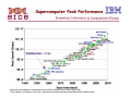
Supercomputer Peak Performance
http://www.reed-electronics.com/electronicnews/article/CA508575.html?indust ryid=21365
From Kilobytes to Petabytes in 50 Years: http://www.eurekalert.org/features/doe/2002-03/dlnl-fkt062102.php
6
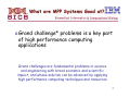
What are MPP Systems Good at?
oGrand challenge* problems is a key part
of high performance computing
applications
Grand challenges are fundamental problems in science
and engineering with broad economic and scientific
impact, and whose solution can be advanced by applying
high performance computing techniques and resources
7
Different from the Rest
8
Source: Pete Beckam, Director, ACLF, Argonne National Lab.
Pushing the Technology
9
Source: Pete Beckam, Director, ACLF, Argonne National Lab.
Machine for Protein Folding
December 1999:
IBM Announces $100 Million Research Initiative to
build World's Fastest Supercomputer
"Blue Gene" to Tackle Protein Folding Grand Challenge
YORKTOWN HEIGHTS, NY, December 6, 1999 -- IBM today announced a new $100 million
exploratory research initiative to build a supercomputer 500 times more powerful than the world’s
fastest computers today. The new computer -- nicknamed "Blue Gene" by IBM researchers -- will
be capable of more than one quadrillion operations per second (one petaflop). This level of
performance will make Blue Gene 1,000 times more powerful than the Deep Blue machine that
beat world chess champion Garry Kasparov in 1997, and about 2 million times more powerful
than today's top desktop PCs.
Blue Gene's massive computing power will initially be used to model the folding of human
proteins, making this fundamental study of biology the company's first computing "grand
challenge" since the Deep Blue experiment. Learning more about how proteins fold is expected
to give medical researchers better understanding of diseases, as well as potential cures.
10
MPP Constraints
oLimits of physical size (floor space)
oPower consumption
oCooling needed to house and run the
aggregated equipment
11
Design Considerations
o Widening gap between processor and DRAM clock
rates
o Excessive heat generated by dense packaging and
high switching frequency
o Disparity between processor clock rate and
immediate vicinity peripheral devices ( memory, I/O
buses, etc. )
o Network performance
The speed of the processor is traded in favor of dense
packaging and low power consumption per processor
12
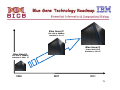
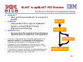
Blue Gene Technology Roadmap
Blue Gene/P
PPC 450 @ 850MHz
Scalable to 3+ PF
Blue Gene/Q
Power Multi-Core
Scalable to 10+ PF
Blue Gene/L
PPC 440 @ 700MHz
Scalable to 360+ TF
2004
2007
2011
13
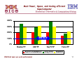
Most Power, Space, and Cooling efficient
Supercomputer
400%
300%
200%
IBM BG/P
100%
0%
Racks/TF
kW/TF
Sun/Constellation
(Published specs per peak performance)
Sq Ft/TF
Cray/XT4
Tons/TF
SGI/ICE
14
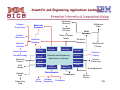
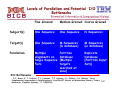
Areas of Application
o Improve understanding – significantly larger scale, more complex and higher
resolution models; new science applications
o Multiscale and multiphysics – From atoms to mega-structures; coupled applications
o Shorter time to solution – Answers from months to minutes
Life Sciences: In-Silico
Trials, Drug Discovery
Geophysical Data Processing
Upstream Petroleum
Biological
Modeling – Brain Science
Physics – Materials Science
Molecular Dynamics
Environment and Climate Modeling
Financial Modeling
Streaming Data Analysis
Computational Fluid Dynamics
Life Sciences: Sequencing
15
Outline
o
Part I: Hardware
–
–
–
o
Historical perspective: Why do we need MPPs?
Overview of massively parallel processing (MPP)
Architecture
Part II: Software
–
–
–
–
Overview
Compilers
MPI
Building and Running Examples on Blue Gene
•
o
Part III: Applications
–
–
–
MPP architecture and its impact on applications
Performance tools
Introduction to code optimization
•
–
–
–
–
–
Hands-on session 2
Mapping applications on a massively parallel architecture
Applications landscape
Challenges and characteristics of Life Sciences applications
Selected Bioinformatics applications
Selected Structural Biology applications
•
o
o
Hands-on session 1
Hands-on session 3
Summary
Biomedical Informatics and Computational Biology (BICB)
16
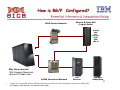
How is BG/P Configured?
1GbE Service Network
Service & Front End
(Login) Nodes
SLES10
DB2
XLF
XLC/C++
GPFS
ESSL
TWS LL
Blue Gene core rack
1024 Compute Nodes/rack
Up to 64 I/O Nodes/rack
10GbE Functional Network
1.
File
Servers
Source: C. P. Sosa and B. Knutson, IBM System Blue Gene Solution: Blue Gene/P Application Development, SG24-727803 Redbooks, Draft Redbooks, last update 25 August 2009
Storage
Subsystem
17
IBM System Blue Gene/P®
System-on-Chip (SoC)
Quad PowerPC 450 w/ Double FPU
Memory Controller w/ ECC
L2/L3 Cache
DMA & PMU
Torus Network
Collective Network
Global Barrier Network
10GbE Control Network
JTAG Monitor
System
Up to 256 Racks
Up to 3.5 PF/s
Up to 512 TB
Cabled
8x8x16
Rack
32 Node Cards
13.9 TF/s
2 TB
Node Card
SoC
13.6 GF/s
8 MB EDRAM
1.
32 Compute Cards
0-2 I/O cards
Compute Card
435.2 GF/s
1 SoC, 40 DRAMs
64 GB
13.6 GF/s
2 GB DDR
Source: C. P. Sosa and B. Knutson, IBM System Blue Gene Solution: Blue Gene/P Application Development, SG24-727803 Redbooks, Draft Redbooks, last update 25 August 2009
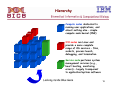
Hierarchy
Compute nodes dedicated to
running user applications, and
almost nothing else – simple
compute node kernel (CNK)
I/O nodes run Linux and
provide a more complete
range of OS services – files,
sockets, process launch,
debugging, and termination
Service node performs system
management services (e.g.,
heart beating, monitoring
errors) – largely transparent
to application/system software
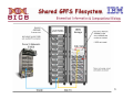
Looking inside Blue Gene
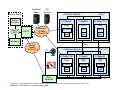
19
Frontend
Nodes
File
Servers
Collective Network
Service Node
System
Console
DB2
CMCS
Functional
10 Gbps
Ethernet
Pset 0
I/OI/O
Node
1151
Node
0
I/OC-Node
Node 1151
0
I/O
I/O Node
Node 1151
1151
Linux
CNK
CNK
fs client
MPI
MPI
ciod
app
app
.
.
Scheduler
Control
Gigabit
Ethernet
.
I2C
torus
. Collective Network
. Node 1151
I/O
I/O Node
1151
Pset 1151
I/OC-Node
Node 1151
0
I/OC-Node
Node 1151
63
Linux
CNK
CNK
. fs client
fs client
fs client
ciod
ciod
.
.
ciod
iCon+
Palomino
1.
Source: C. P. Sosa and B. Knutson, IBM System Blue Gene Solution: Blue Gene/P Application Development, SG24-727803 Redbooks, Draft Redbooks, last update 25 August 2009
JTAG
Shared GPFS Filesystem
21
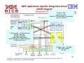
BG/P Applications Specific Integrated Circuit
(ASIC) Diagram
L2 Data cache:
prefetch buffer
holds 15 128128-byte lines can prefetch
up to 7 streams
L1 Data cache : 32 KB total size
3232-Byte line size,
6464-way associative
roundround-robin replacement
writewrite-through for cache coherency
4-cycle load to use
L3 Data cache : 2x4 MB
~50 cycles latency
onon-chip
22
1.
Source: C. P. Sosa and B. Knutson, IBM System Blue Gene Solution: Blue Gene/P Application Development, SG24-727803 Redbooks, Draft Redbooks, last update 25 August 2009
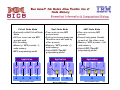
Blue Gene/P Job Modes Allow Flexible Use of
Node Memory
Dual Node Mode
o Two cores run one MPI
process each
o Each process may spawn one
thread on core not used by
other process
o Memory / MPI process = ½
node memory
o Hybrid MPI/OpenMP
programming model
M
M
Memory address space
M
M
T
M
Memory address space
CPU2
T
CPU3
T
Core 3
P
Core 0
T
P
Core 2
P
Application
Core 3
Core 1
P
Core 0
Core 2
Core 0
M
P
Core 3
P
Core 1
P
Application
Core 2
Application
SMP Node Mode
o One core runs one MPI
process
o Process may spawn threads
on each of the other cores
o Memory / MPI process = full
node memory
o Hybrid MPI/OpenMP
programming model
Core 1
Virtual Node Mode
oPreviously called Virtual Node
Mode
oAll four cores run one MPI
process each
oNo threading
oMemory / MPI process = ¼
node memory
oMPI programming model
T
M
Memory address space
23
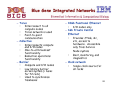
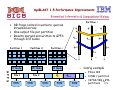
Blue Gene Integrated Networks
– Torus
•
Interconnect to all
compute nodes
•
Torus network is used
•
Point-to-point
communication
– Collective
•
Interconnects compute
and I/O nodes
•
One-to-all broadcast
functionality
•
Reduction operations
functionality
– Barrier
•
Compute and I/O nodes
•
Low latency barrier
across system (< 1usec
for 72 rack)
•
Used to synchronize
timebases
– 10Gb Functional Ethernet
•
I/O nodes only
– 1Gb Private Control
Ethernet
•
Provides JTAG, i2c,
etc, access to
hardware. Accessible
only from Service
Node system
•
Boot, monitoring, and
diagnostics
– Clock network
•
Single clock source for
all racks
24
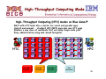
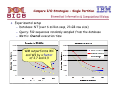
High-Throughput Computing Mode
High-Throughput Computing (HTC) modes on Blue Gene/P
BG/P with HTC looks like a cluster for serial and parallel apps
Hybrid environment … standard HPC (MPI) apps plus now HTC apps
Enables a new class of workloads that use many single-node jobs
Easy administration using web-based Navigator
HTC
App6
App9
App8
App8
App1
App1
App1
App1
App7
App8
App9
App6
App1
App1
App1
App1
App6
App8
App8
App9
App1
App1
App1
App1
App7
App7
App9
App6
App1
App1
App1
App1
HTC VNM
512 nodes
HTC DM
256 nodes
HTC SMP
256 nodes
HPC
1024 nodes
HPC
25
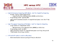
HPC versus HTC
o
High Performance Computing (HPC) Mode – best for Capability Computing
– Parallel, tightly coupled applications
• Single Instruction, Multiple Data (SIMD) architecture
– Programming model: typically MPI
– Apps need tremendous amount of computational power over short time
period
o
High Throughput Computing (HTC) Mode – best for Capacity Computing
– Large number of independent tasks
• Multiple Instruction, Multiple Data (MIMD) architecture
– Programming model: non-MPI
– Apps need large amount of computational power over long time period
– Traditionally run on large clusters
o
HTC and HPC modes co-exist on Blue Gene
– Determined when resource pool (partition) is allocated
26
Outline
o
Part I: Hardware
–
–
–
o
Historical perspective: Why do we need MPPs?
Overview of massively parallel processing (MPP)
Architecture
Part II: Software
–
–
–
–
Overview
Compilers
MPI
Building and Running Examples on Blue Gene
•
o
Part III: Applications
–
–
–
MPP architecture and its impact on applications
Performance tools
Introduction to code optimization
•
–
–
–
–
–
Hands-on session 2
Mapping applications on a massively parallel architecture
Applications landscape
Challenges and characteristics of Life Sciences applications
Selected Bioinformatics applications
Selected Structural Biology applications
•
o
o
Hands-on session 1
Hands-on session 3
Summary
Biomedical Informatics and Computational Biology (BICB)
27
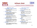
Software Stack
o
o
o
o
o
IBM Software Stack
XL (FORTRAN, C, and C++) compilers
Externals preserved
Optimized for specific BG functions
OpenMP support
LoadLeveler scheduler
Same externals for job submission
and system query functions
Backfill scheduling to achieve
maximum system utilization
GPFS parallel file system
Provides high performance file
access, as in current pSeries and
xSeries clusters
Runs on I/O nodes and disk servers
ESSL/MASSV libraries
Optimization library and intrinsics
for better application performance
Serial Static Library supporting 32bit applications
Callable from FORTRAN, C, and C++
MPI library
Message passing interface library,
based on MPICH2, tuned for the Blue
Gene architecture
o
o
o
o
o
Other Software Support
Parallel File Systems
Lustre at LLNL, PVFS2 at ANL
Job Schedulers
SLURM at LLNL, Cobalt at ANL
Altair PBS Pro, Platform LSF (for
BG/L only)
Condor HTC (porting for BG/P)
Parallel Debugger
Etnus TotalView (for BG/L as of now,
porting for BG/P)
Allinea DDT and OPT (porting for
BG/P)
Libraries
FFT Library - Tuned functions by
TU-Vienna
VNI (porting for BG/P)
Performance Tools
HPC Toolkit: MP_Profiler, Xprofiler,
HPM, PeekPerf, PAPI
Tau, Paraver, Kojak
28
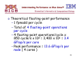
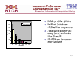
Understanding Performance on Blue Gene/P
o Theoretical floating-point performance
– 1 fpmadd per cycle
– Total of 4 floating-point operations
per cycle
– 4 floating-point operations/cycle x
850 cycle/s x 106 = 3,400 x 106 = 3.4
GFlop/s per core
– Peak performance = 13.6 GFlop/s per
node ( 4 cores )
29
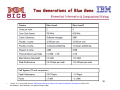
Two Generations of Blue Gene
30
1.
Source: C. P. Sosa and B. Knutson, IBM System Blue Gene Solution: Blue Gene/P Application Development, SG24-727803 Redbooks, Draft Redbooks, last update 25 August 2009
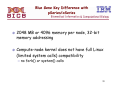
Blue Gene Key Difference with
pSeries/xSeries
o 2048 MB or 4096 memory per node, 32-bit
memory addressing
o Compute-node kernel does not have full Linux
(limited system calls) compatibility
– no fork() or system() calls
31
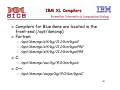
IBM XL Compilers
o Compilers for Blue Gene are located in the
front-end (/opt/ibmcmp)
o Fortran:
– /opt/ibmcmp/xlf/bg/11.1/bin/bgxlf
– /opt/ibmcmp/xlf/bg/11.1/bin/bgxlf90
– /opt/ibmcmp/xlf/bg/11.1/bin/bgxlf95
o C:
– /opt/ibmcmp/vac/bg/9.0/bin/bgxlc
o C++:
– /opt/ibmcmp/vacpp/bg/9.0/bin/bgxlC
32
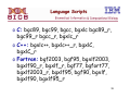
Language Scripts
o C: bgc89, bgc99, bgcc, bgxlc bgc89_r,
bgc99_r bgcc_r, bgxlc_r
o C++: bgxlc++, bgxlc++_r, bgxlC,
bgxlC_r
o Fortran: bgf2003, bgf95, bgxlf2003,
bgxlf90_r, bgxlf_r, bgf77, bgfort77,
bgxlf2003_r, bgxlf95, bgf90, bgxlf,
bgxlf90, bgxlf95_r
33
Unsupported Options
The following compiler options, although
available for other IBM systems, are not
supported by the Blue Gene/P hardware
o -q64: The Blue Gene/P system uses a 32-bit
architecture; you cannot compile in 64-bit
mode
o -qaltivec: The 450 processor does not
support VMX instructions or vector data
types.
34
GNU Compilers
o The Standard GNU compilers and libraries which are also
located on the frontend node will NOT produce Blue Gene
compatible binary code. The standard GNU compilers can only be
used for utility or frontend code development that your
application may require.
o GNU compilers (Fortran, C, C++) for Blue Gene are located in
(/opt/blrts-gnu/ )
o Fortran:
– /opt/gnu/powerpc-bgp-linux-gfortran
o C:
– /opt/gnu/powerpc-bgp-linux-gcc
o C++:
– /opt/gnu/powerpc-bgp-linux-g++
o It is recommended not to use GNU compiler for Blue Gene as
the IBM XL compilers offer significantly higher performance.
The GNU compilers do offer more flexible support for things
like inline assembler.
35
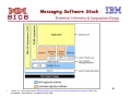
Messaging Software Stack
36
1.
Source: C. P. Sosa and B. Knutson, IBM System Blue Gene Solution: Blue Gene/P Application Development, SG24-727803 Redbooks, Draft Redbooks, last update 25 August 2009
MPI Library Location
o MPI implementation on Blue Gene is based
on MPICH-2 from Argonne National
Laboratory
o Include files mpi.h and mpif.h are at the
location:
– I/bgsys/drivers/ppcfloor/comm/include
37
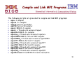
Compile and Link MPI Programs
The following scripts are provided to compile and link MPI programs:
o
o
o
o
o
o
o
o
o
o
o
o
o
o
o
o
o
mpicc C compiler
mpicxx C++ compiler
mpif77 Fortran 77compiler
mpif90 Fortran 90 compiler
mpixlc IBM XL C compiler
mpixlc_r Thread-safe version of mpixlc
mpixlcxx IBM XL C++ compiler
mpixlcxx_r Thread-safe version of mpixlcxx
mpixlf2003 IBM XL Fortran 2003 compiler
mpixlf2003_r Thread-safe version of mpixlf2003
mpixlf77 IBM XL Fortran 77 compiler
mpixlf77_r Thread-safe version of mpixlf77
mpixlf90 IBM XL Fortran 90 compiler
mpixlf90_r Thread-safe version of mpixlf90
mpixlf95 IBM XL Fortran 95 compiler
mpixlf95_r Thread-safe version of mpixlf95
mpich2version Prints MPICH2 version information
38
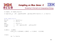
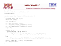
Compiling on Blue Gene: C
$ make -f make.hello
$ mpixlc_r -O3 -qarch=450 -qtune=450 hello.c -o hello
$cat make.hello
XL_CC
= mpixlc_r
OBJ
= hello
SRC
= hello.c
FLAGS
= -O3 -qarch=450
LIBS
=
$(OBJ):
-qtune=450
$(SRC)
${XL_CC} $(FLAGS) $(SRC) -o $(OBJ)
$(LIBS)
clean:
rm *.o hello
39
Hello World: C
$ cat hello.c
#include <stdio.h>
#include "mpi.h"
/* Headers
*/
main(int argc, char **argv) /* Function main
{
int rank, size, tag, rc, i;
MPI_Status status;
char message[20];
*/
rc = MPI_Init(&argc, &argv);
rc = MPI_Comm_size(MPI_COMM_WORLD, &size);
rc = MPI_Comm_rank(MPI_COMM_WORLD, &rank);
tag = 100;
if(rank == 0) {
strcpy(message, "Hello, world");
for (i=1; i<size; i++)
rc = MPI_Send(message, 13, MPI_CHAR, i, tag, MPI_COMM_WORLD);
}
else
rc = MPI_Recv(message, 13, MPI_CHAR, 0, tag, MPI_COMM_WORLD, &status);
printf( "node %d : %.13s\n", rank,message);
rc = MPI_Finalize();
}
40
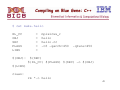
Compiling on Blue Gene: C++
$ cat make.hello
XL_CC
OBJ
SRC
FLAGS
LIBS
$(OBJ):
=
=
=
=
=
mpixlcxx_r
hello
hello.cc
-O3 -qarch=450
-qtune=450
$(SRC)
${XL_CC} $(FLAGS) $(SRC) -o $(OBJ)
$(LIBS)
clean:
rm *.o hello
41
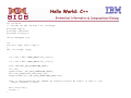
Hello World: C++
cat hello.cc
// Include the MPI version 2 C++ bindings:
#include <mpi.h>
#include <iostream>
#include <string.h>
using namespace std;
int
main(int argc, char* argv[])
{
MPI::Init(argc, argv);
int rank = MPI::COMM_WORLD.Get_rank();
int size = MPI::COMM_WORLD.Get_size();
char name[MPI_MAX_PROCESSOR_NAME];
int len;
memset(name,0,MPI_MAX_PROCESSOR_NAME);
MPI::Get_processor_name(name,len);
memset(name+len,0,MPI_MAX_PROCESSOR_NAME-len);
cout << "hello_parallel.cc: Number of tasks="<<size<<" My rank=" << rank << " My
name="<<name<<"."<<endl;
MPI::Finalize();
return 0;
}
42
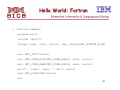
Hello World: Fortran
c
Fortran example
program hello
include 'mpif.h'
integer rank, size, ierror, tag, status(MPI_STATUS_SIZE)
call MPI_INIT(ierror)
call MPI_COMM_SIZE(MPI_COMM_WORLD, size, ierror)
call MPI_COMM_RANK(MPI_COMM_WORLD, rank, ierror)
print*, 'node', rank, ': Hello world'
call MPI_FINALIZE(ierror)
end
43
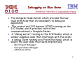
Debugging on Blue Gene
o The Compute Node Kernel, which provides the lowlevel primitives that are necessary to debug an
application
o The control and I/O daemon (CIOD) running on the
I/O Nodes, which provides control and
communications to Compute Nodes
o A “debug server” running on the I/O Nodes, which is
vendor-supplied code that interfaces with the CIOD
o A debug client running on a Front End Node, which is
where the user does their work interactively
– GNU Project debugger
– Core processor debugger
– Addr2Line utility
44
Outline
o
Part I: Hardware
–
–
–
o
Historical perspective: Why do we need MPPs?
Overview of massively parallel processing (MPP)
Architecture
Part II: Software
–
–
–
–
Overview
Compilers
MPI
Building and Running Examples on Blue Gene
•
o
Part III: Applications
–
–
–
MPP architecture and its impact on applications
Performance tools
Introduction to code optimization
•
–
–
–
–
–
Hands-n session 2
Mapping applications on a massively parallel architecture
Applications landscape
Challenges and characteristics of Life Sciences applications
Selected Bioinformatics applications
Selected Structural Biology applications
•
o
o
Hands-on session 1
Hands-on session 3
Future Directions
Summary
45
Hardware Naming Convention
46
1.
Source: C. P. Sosa and B. Knutson, IBM System Blue Gene Solution: Blue Gene/P Application Development, SG24-727803 Redbooks, Draft Redbooks, last update 25 August 2009
Cards Naming Convention
47
Submitting Jobs: mpirun
o Job submission using mpirun
– User can use “mpirun” to submit jobs.
– The Blue Gene mpirun is located in /usr/bin/mpirun
o Typical use of mpirun :
– mpirun -np <# of processes> -partition <block id> -cwd `pwd` -exe
<executable>
o Where:
-np : Number of processors to be used. Must fit in available partition
-partition : A partition from Blue Gene rack on which a given executable will
execute, eg., R000.
-cwd : The current working directory and is generally used to specify where
any input and output files are located.
-exe : The actual binary program which user wish to execute.
Example :
mpirun -np 32 -partition R000 -cwd /gpfs/fs2/frontend11/myaccount -exe /gpfs/fs2/frontend-11/myaccount/hello
48
mpirun Standalone Versus mpirun in LL
Environment
Comparison between mpirun and Loadleveler llsubmit command command
job_type and requirements tags must ALWAYS be specified as
listed above
If the above command file listing were contained in a file named
my_job.cmd, then the job would then be submitted to the LoadLeveler
49
queue using llsubmit my_job.cmd.
Outline
o
Part I: Hardware
–
–
–
o
Historical perspective: Why do we need MPPs?
Overview of massively parallel processing (MPP)
Architecture
Part II: Software
–
–
–
–
Overview
Compilers
MPI
Building and Running Examples on Blue Gene
•
o
Part III: Applications
–
–
–
MPP architecture and its impact on applications
Performance tools
Introduction to code optimization
•
–
–
–
–
–
Hands-n session 2
Mapping applications on a massively parallel architecture
Applications landscape
Challenges and characteristics of Life Sciences applications
Selected Bioinformatics applications
Selected Structural Biology applications
•
o
o
Hands-on session 1
Hands-on session 3
Future Directions
Summary
50
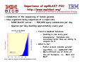
American Chemical Society: Chemical & Engineering News:
April 13, 2009 Issue
April 13, 2009
o “The Looming Petascale”
o “Chemists gear up for a new
generation of supercomputers”
o “The new petascale computers will
be 1,000 times faster than the
terascale supercomputers of today,
performing more than 1,000 trillion
operations per second. And instead
of machines with thousands of
processors, petascale machines will
have many hundreds of thousands
that simultaneously process streams
of information.”
http://pubs.acs.org/cen/science/87/8715sci3.html
o “This technological sprint could be a
great boon for chemists, allowing
them to computationally explore the
structure and behavior of bigger
and more complex molecules.”
51
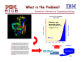
What is the Challenge?
Applications …
… are we there?
52
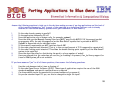
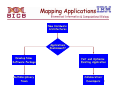
Porting Applications to Blue Gene
Answer the following questions to help you in the decision-making process of porting applications and the level of
effort required (answering “yes” to most of the questions is an indication that your code is already
enabled for distributed-memory systems and a good candidate for Blue Gene/P):
1.
2.
3.
4.
5.
6.
7.
8.
9.
Is the code already running in parallel?
Is the application addressing 32-bit?
Does the application rely on system calls, for example, system?
Does the code use the Message Passing Interface (MPI), specifically MPICH? Of the several parallel
programming APIs, the only one supported on the Blue Gene/P system that is portable is MPICH.
OpenMP is supported only on individual nodes.
Is the memory requirement per MPI task less than 4 GB?
Is the code computational intensive? That is, is there a small amount of I/O compared to computation?
Is the code floating-point intensive? This allows the double floating-point capability of the Blue Gene/P
system to be exploited.
Does the algorithm allow for distributing the work to a large number of nodes?
Have you ensured that the code does not use flex_lm licensing? At present, flex_lm library support for
Linux on IBM System p® is not available.
If you have answered “yes” to all of these questions, then answer the following questions:
1.
2.
3.
4.
Has the code been ported to Linux on System p?
Is the code Open Source Software (OSS)? These type of applications require the use of the GNU
standard configure and special considerations are required
Can the problem size be increased with increased numbers of processors?
Do you use standard input? If yes, can this be changed to single file input?
53
What is Performance Tuning?
o Application (software) optimization is
the process of making it work more
efficiently
– Executes faster
– Uses less memory
– Performs less I/O
– Better use of resources
Robert Sedgewick, Algorithms, 1984, p. 84
Programming Optimization: http://www.azillionmonkeys.com/qed/optimize.html
54
Application Flow Analysis
Work
Tasks
Time
55
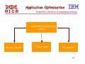
Application Optimization
Application performance
analysis
Memory bound?
I/O bound?
CPU bound?
56
Optimization Steps
1. Tune for compiler optimization flags
2. Locate hot-spots in the code
3. Use highly tuned libraries
MASS/ESSL
4. Manually optimize the code
5. Determine if I/O plays a role and tune
if needed
57
Two Key Concepts
o Speedup
o Efficiency
58
Speedup
o Speedup is defined as the ratio between
the run time of the original code and
the run time of the modified code
Original code run time
Speedup =
Modified code run time
59
Parallel Speedup
o Parallel speedup is defined as the ratio
between the run time of the sequential
code and the run time of the modified
code
Sequential run time
Parallel Speedup =
Parallel run time
Run time is measured as elapsed time ( or wallclock)
60
Efficiency
o Parallel efficiency is defined as how well
a program (your code) utilizes multiple
processors (cores)
Sequential run time
Efficiency
=
Nprocessors X Parallel run time
N is the number of processors defined by the user
61
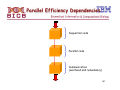
Parallel Efficiency Dependencies
Sequential code
Parallel code
Communication
(overhead and redundancy)
62
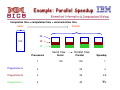
Example: Parallel Speedup
Completion time = computation time + communication time
Serial
Parallel
25
100
35
45
Serial time
Processors
Serial
1
100
Parallel time
Parallel
Speedup
100
1
Programmer A
4
25
4
Programmer B
4
35
2.9
Programmer c
4
45
63
2.2
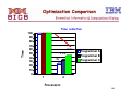
Optimization Comparison
Time
Time reduction
100
90
80
70
60
50
40
30
20
10
0
2.2x
2.9x
4x
1
Programmer A
Programmer B
Programmer C
4
Processors
64
Outline
o
Part I: Hardware
–
–
–
o
Historical perspective: Why do we need MPPs?
Overview of massively parallel processing (MPP)
Architecture
Part II: Software
–
–
–
–
Overview
Compilers
MPI
Building and Running Examples on Blue Gene
•
o
Part III: Applications
–
–
–
MPP architecture and its impact on applications
Performance tools
Introduction to code optimization
•
–
–
–
–
–
Hands-n session 2
Mapping applications on a massively parallel architecture
Applications landscape
Challenges and characteristics of Life Sciences applications
Selected Bioinformatics applications
Selected Structural Biology applications
•
o
o
Hands-on session 1
Hands-on session 3
Future Directions
Summary
65
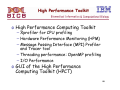
High Performance Toolkit
o High Performance Computing Toolkit
– Xprofiler for CPU profiling
– Hardware Performance Monitoring (HPM)
– Message Passing Interface (MPI) Profiler
and Tracer tool
– Threading performance: OpenMP profiling
– I/O Performance
o GUI of the High Performance
Computing Toolkit (HPCT)
66
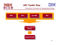
HPC Toolkit Flow
HPM
HPM
MPI
MPI
OpenMP
OpenMP
MIO
MIO
CC/ /C++
C++/Fortran
/Fortran
Binary
Binary
Output/Analysis
Output/Analysis
67
CPU Profiling using Xprofiler
o Xprofiler:
– Used to analyze your application performance
– It uses data collected by the -pg compiler option
to construct a graphical display
– It identifies functions that are the most CPU
intensive
o GUI manipulates the display in order to focus
on the critical areas of the application
o Important factors:
– Sampling interval is in the order of ms
– Profiling introduces overhead due to function calls
68
Starting Xprofiler
o Start Xprofiler by issuing the Xprofiler command
from the command line
– Specify the executable
– Profile data file or files
– Options
• Specify them on the command line, with the Xprofiler command
• Issue the Xprofiler command alone and then specify the options
from within the GUI
o $Xprofiler a.out gmon.out... [options]
– a.out is the name of your binary executable file
– gmon.out is the name of your profile data file or files
– options
69
Xprofiler versus gprof
o Xprofiler gives a graphical picture of the CPU consumption of
your application in addition to textual data
o Xprofiler displays your profiled program in a single main window
o It uses several types of graphic images to represent the
relevant parts of your program:
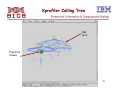
– Functions are displayed as solid green boxes, called function boxes
– Calls between them are displayed as blue arrows, called call arcs
– The function boxes and call arcs that belong to each library within
your application are displayed within a fenced-in area called a
cluster box
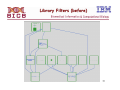
o When Xprofiler first opens, by default, the function boxes for
your application are clustered by library. This type of clustering
means that a cluster box appears around each library, and the
function boxes and call arcs within the cluster box are reduced
in size.
– If you want to see more detail, you must uncluster the functions by
selecting File → Uncluster Functions
70
Xprofiler Main Menus
o File menu
–
o
View menu
–
o
Using the Filter menu, you can add, remove, and change specific parts of the function
call tree. By controlling what Xprofiler displays, you can focus on the objects that are
most important to you.
Report menu
–
o
You use the View menu to help you focus on portions of the function call tree, in the
Xprofiler main window, in order to have a better view of the application’s critical areas.
Filter menu
–
o
With the File menu, you specify the executable (a.out) files and profile data (gmon.out)
files that Xprofiler will use. You also use this menu to control how your files are
accessed and saved.
The Report menu provides several types of profiled data in a textual and tabular
format. With the options of the Report menu, you can display textual data, save it to a
file, view the corresponding source code, or locate the corresponding function box or
call arc in the function call tree, in addition to presenting the profiled data.
Utility menu
–
The Utility menu contains one option, Locate Function By Name, with which you can
highlight a particular function box in the function call tree.
71
Xprofiler Main Menus - 2
o Function menu
–
–
Number of operations for any of the functions shown in the function call tree by using
the Function menu. You can access statistical data, look at source code, and control
which functions are displayed
The Function menu is not visible from the Xprofiler window. To access it, you right-click
the function box of the function in which you are interested
o Arc menu
–
–
Locate the caller and callee functions for a particular call arc
The Arc menu is not visible from the Xprofiler window. You access it by right-clicking
the call arc in which you are interested
o Cluster Node menu
–
–
–
Control the way your libraries are displayed by Xprofiler
The Cluster Node menu is not visible from the Xprofiler window. You access it by rightclicking the edge of the cluster box in which you are interested.
Display Status Field at the bottom of the Xprofiler window is a single field that tells
you:
• The name of your application
• The number of gmon.out files used in this session
• The total amount of CPU used by the application
• The number of functions and calls in your application and how many are currently
displayed
72
Building AMBER7 with Xprofiler
########## LOADER/LINKER:
# Use Standard options
setenv LOAD "xlf90 -pg -bmaxdata:0x80000000 "
# Load with the IBM MASS & ESSL libraries
setenv LOADLIB " "
if ( $HAS_MASSLIB == "yes" ) setenv LOADLIB "-L$MASSLIBDIR -lmassvp4 "
if ( $VENDOR_BLAS == "yes" ) setenv LOADLIB "$LOADLIB -lblas "
if ( $VENDOR_LAPACK == "yes" ) setenv LOADLIB "$LOADLIB -lessl "
# little or no optimization:
setenv L0 "xlf90 -pg -qfixed -c"
# modest optimization (local scalar):
setenv L1 "xlf90 -pg -qfixed -O2 -c"
# high scalar optimization (but not vectorization):
setenv L2 "xlf90 -pg -qfixed -O3 -qmaxmem=-1 -qarch=auto -qtune=auto -c"
# high optimization (may be vectorization, not parallelization):
setenv L3 "xlf90 -pg -qfixed -O3 -qmaxmem=-1 -qarch=auto -qtune=auto -c"
73
Xprofiler Calling Tree
Call
arcs
Function
boxes
74
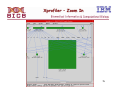
Xprofiler – Zoom In
75
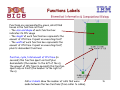
Functions Labels
Functions are represented by green, solid-filled
boxes in the function call tree:
• The size and shape of each function box
indicates its CPU usage
• The height of each function box represents the
amount of CPU time it spent on executing itself
• The width of each function box represents the
amount of CPU time it spent on executing itself,
plus its descendant functions
Function, cycle, total amount of CPU time (in
seconds) this function spent on itself plus
descendants (the number to the left of the x),
the amount of CPU time (in seconds) this function
spent only on itself (the number to the right of
the x)
Call arc labels show the number of calls that were
made between the two functions (from caller to callee).
76
Library Filters (before)
77
Library Filters (after)
78
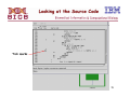
Looking at the Source Code
Tick marks
79
Looking at Assembler Code
80
Xprofiler – Flat Format
%time
55.0
9.1
8.1
6.2
[13]
cumulative
seconds
16.53
19.27
21.71
23.57
self
seconds
calls
16.53
2.74
2.44
1.86
235580
23558
10
10
self total
ms/call
ms/call
0.07
0.12
244.00
186.00
0.07
0.12
244.00
190.00
name
.short_ene [7]
.pack_nb_list [11]
.grad_sumrc [12]
.fill_charge_grid
81
Mass Library
o Mathematical Acceleration Subsystem (MASS)
consists of libraries of tuned mathematical intrinsic
functions
o Scalar Library: The MASS scalar library, libmass.a,
contains an accelerated set of frequently used math
intrinsic functions in the AIX and Linux system
library libm.a (now called libxlf90.a in the IBM XL
Fortran manual): o sqrt, rsqrt, exp, log, sin, cos, tan,
atan, atan2, sinh, cosh, tanh, dnint, x**y
o Vector Library: The general vector library, libmassv.a,
contains vector functions that will run on the entire
IBM pSeries and Blue Gene families.
82
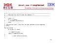
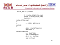
short_ene.f unoptimized
c-------------------------------------------------------------------------c
Loop over the 12-6 LJ terms for eedmeth = 1
c-------------------------------------------------------------------------c
icount = 0
do m = 1,numvdw
#
include "ew_directp.h"
enddo
c
c calculation starts: loop over the data gathered in the temporary
c array.
c
C*$* NO FUSION
do im_new = 1,icount
j = tempint(im_new)
delr2 = tempre(5*im_new)
c
c
-- cubic spline on switch:
83
short_ene.f unoptimized (cont.)
c
delrinv= 1.0/sqrt(delr2)
delr = delr2*delrinv
delr2inv = delrinv*delrinv
x = dxdr*delr
ind = eedtbdns*x
dx = x - ind*del
ind = 4*ind
$
e3dx = dx*eed_cub(3+ind)
e4dx = dx*dx*eed_cub(4+ind)
switch = eed_cub(1+ind) + dx*(eed_cub(2+ind) +
(e3dx + e4dx*third)*half)
d_switch_dx = eed_cub(2+ind) + e3dx+ e4dx*half
c
84
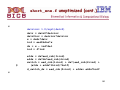
short_ene.f optimized
c-------------------------------------------------------------------------c
Loop over the 12-6 LJ terms for eedmeth = 1
c-------------------------------------------------------------------------c
icount = 0
do m = 1,numvdw
#
include "ew_directp.h"
enddo
c
c calculation starts: loop over the data gathered in the temporary
c array caches.
c
#ifdef MASSLIB
call vrsqrt( cache_df, cache_r2, icount )
#else
do im_new = 1,icount
delr2 = cache_r2(im_new)
delrinv = 1.0/sqrt(delr2)
cache_df(im_new) = delrinv
enddo
#endif
85
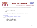
short_ene.f optimized (cont.)
do im_new = 1,icount
j = cache_bckptr(im_new)
delr2 = cache_r2(im_new)
delrinv =
cache_df(im_new)
c
c
-- cubic spline on
switch:
c
delr = delr2*delrinv
delr2inv =
delrinv*delrinv
x = dxdr*delr
ind = eedtbdns*x
dx = x - ind*del
ind = 4*ind
86
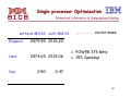
Single processor Optimization
without MASS with MASS
Elapsed
User
Sys
vector mass
2579.95 2226.20
2574.65 2224.06
0.50
o POWER 375 MHz
o 15% Speedup
0.47
87
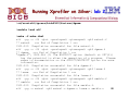
Running Xprofiler on Silver: lab 2
%cd/scratch1/cpsosa/bicb8510/fortran/dgemm
%module load xlf
%make -f make.ibm1
xlf -pg -c -O3 -qhot -qarch=pwr6 -qtune=pwr6 -q64 matmul.f
** matmul
=== End of Compilation 1 ===
1501-510 Compilation successful for file matmul.f.
xlf -pg -c -O3 -qhot -qarch=pwr6 -qtune=pwr6 -q64 dgemm.f
** dgemm
=== End of Compilation 1 ===
"dgemm.f", 1500-036 (I) The NOSTRICT option (default at OPT(3))
has the potential to alter the semantics of a program. Please
refer to documentation on the STRICT/NOSTRICT option for more
information.
1501-510 Compilation successful for file dgemm.f.
xlf -pg -c -O3 -qhot -qarch=pwr6 -qtune=pwr6 -q64 lsame.f
** lsame
=== End of Compilation 1 ===
1501-510 Compilation successful for file lsame.f.
xlf -pg -c -O3 -qhot -qarch=pwr6 -qtune=pwr6 -q64 xerbla.f
** xerbla
=== End of Compilation 1 ===
1501-510 Compilation successful for file xerbla.f.
xlf -pg -o matmul -q64 matmul.o dgemm.o lsame.o xerbla.o
88
Running Xprofiler on Silver: lab 2-2
%./matmul
mflops are 964.993481618238206
%ls
dgemm.f gmon.out lsame.o matmul
matmul.o xerbla.o
dgemm.o lsame.f make.ibm1 matmul.f
xerbla.f
%module load hpct
%Xprof ./matmul gmon.out
89
Running Xprofiler: lab 2-3
90
Hardware Performance Monitor (HPM) & Prerequisities
o Hardware Performance Counter:
– Set of special-purpose “registers” built into
modern “microprocessors” to store the
“To understand what
happens
counts of hardware-related
activities
inside a processor when an
within computer
systems
application is executed,
• Advanced users
oftenarchitects
rely on those
counters
processor
designed
a to
performance
analysis
or
conduct “low-level
set of special
registers
to count
tuning”
the events taking
place when processors are
http://en.wikipedia.org/wiki/Hardware_performance_counter
executing instructions”
http://download.boulder.ibm.com/ibmdl/pub/software/dw/aix/au-counteranalyzer/au-counteranalyzer-pdf.pdf
91
Registers, Microprocessors, and Tuning
o Processor register (or general purpose
register) is a small amount of storage
available on the CPU whose contents can be
accessed more quickly than storage available
elsewhere http://en.wikipedia.org/wiki/Processor_register
o Microprocessor incorporates most or all of
the functions of a central processing unit
(CPU) on a single integrated circuit (IC)
http://en.wikipedia.org/wiki/Microprocessor
o Performance tuning is the improvement of
system performance
http://en.wikipedia.org/wiki/Performance_tuning
92
Software Profilers
versus Hardware Counters
o Hardware counters provide low-overhead access to a wealth of
detailed performance information related to CPU's functional
units, caches and main memory
o With hardware counters no source code modifications are
needed in general
o Meaning of hardware counters vary from one kind of
architecture to another due to the variation in hardware
organizations
o Difficulties correlating the low level performance metrics back
to source code
o Limited number of registers to store the counters often force
users to conduct multiple measurements to collect all desired
performance metrics
o Modern superscalar processors schedule and execute multiple
instructions at one time
http://en.wikipedia.org/wiki/Hardware_performance_counter
93
Summary of Hardware Counters
o Extra logic inserted in the processor to count
specific events
o Updated at every cycle
o Strengths:
– Non-intrusive
– Very accurate
– Low overhead
o Weakness
–
–
–
–
Provides only hard counts
Specific for each processor
Access is not well documented
Lack of standard and documentation on what is counted
94
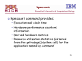
hpmcount
o hpmcount command provides:
– Execution wall clock time
– Hardware performance counters
information
– Derived hardware metrics
– Resource utilization statistics (obtained
from the getrusage() system call) for the
application named by command
95
hpmcount [options]
o -a Aggregates the counters on POE runs
o -d Adds detailed set counts for counter multiplexing
mode
o -H Adds hypervisor activity on behalf of the process
o -h Displays help message
o -k Adds system activity on behalf of the process
o -o file Output file name
o -s set Lists a predefined set of events or a commaseparated list of sets (1 to N, or 0 to select all.
http://publib.boulder.ibm.com/infocenter/pseries/v5r3/index.jsp?topic=/com.ibm.aix.cmds/doc/aixcmds2/hpmcount.htm
96
hpmcount: examples
o
To run the ls command and write information
concerning events in set 5 from hardware
counters, enter:
–
o
hpmcount -s 5 ls
To run the ls command and write information
concerning events in sets 5, 2, and 9 from
hardware counters using the counter
multiplexing mode, enter:
–
hpmcount -s 5,2,9 ls
97
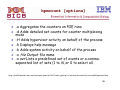
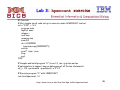
Lab 3: hpmcount exercise
#! /bin/csh
# Very simple serial code set up to execute under HPMCOUNT control.
cat << 'EOF' > ./it.f
program main
implicit none
integer i
real sum
common sum
sum=0.0
do i=1,1000000
sum=sum+exp(.00000001*i)
end do
print*,'sum=',sum
stop
end
'EOF'
# Compile and build program "it" from it.f, use -g option and no
# optimization to support source debugging of all Fortan statements:
xlf_r -O4 -qarch=auto -qrealsize=8 -o it it.f
# Execute program "it" with HPMCOUNT:
/usr/bin/hpmcount ./it
http://www.cisl.ucar.edu/docs/ibm/hpm.toolkit/hpmcount.html
98
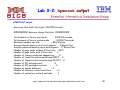
Lab 3-2: hpmcout output
HPMCOUNT output:
Execution time (wall clock time): 0.057595 seconds
######## Resource Usage Statistics ########
Total amount of time in user mode
: 0.015934 seconds
Total amount of time in system mode
: 0.003379 seconds
Maximum resident set size
: 8532 Kbytes
Average shared memory use in text segment : 0 Kbytes*sec
Average unshared memory use in data segment : 77 Kbytes*sec
Number of page faults without I/O activity : 2073
Number of page faults with I/O activity
:2
Number of times process was swapped out
:0
Number of times file system performed INPUT : 0
Number of times file system performed OUTPUT : 0
Number of IPC messages sent
:0
Number of IPC messages received
:0
Number of signals delivered
:0
Number of voluntary context switches
: 13
Number of involuntary context switches
:3
http://www.cisl.ucar.edu/docs/ibm/hpm.toolkit/hpmcount.html
99
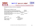
Lab 3-3: hpmcout output
####### End of Resource Statistics ########
Set: 1
Counting duration: 0.019886103 seconds
PM_FPU_1FLOP (FPU executed one flop instruction )
:
4000225
PM_FPU_FMA (FPU executed multiply-add instruction)
:
11000076
PM_FPU_FSQRT_FDIV (FPU executed FSQRT or FDIV instruction) :
0
PM_CYC (Processor cycles)
:
26428653
PM_RUN_INST_CMPL (Run instructions completed)
:
47657875
PM_RUN_CYC (Run cycles)
:
93529315
Utilization rate
Flop
Flop rate (flops / WCT)
Flops / user time
FMA percentage
:
:
9.755 %
26.000 Mflop
:
451.435 Mflop/s
:
4627.772 Mflop/s
:
146.665 %
http://www.cisl.ucar.edu/docs/ibm/hpm.toolkit/hpmcount.html
100
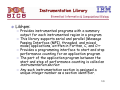
Instrumentation Library
o Libhpm:
– Provides instrumented programs with a summary
output for each instrumented region in a program
– This library supports serial and parallel (Message
Passing Interface (MPI), threaded, and mixed
mode) applications, written in Fortran, C, and C++
– Provides a programming interface to start and stop
performance counting for an application program
– The part of the application program between the
start and stop of performance counting is called an
instrumentation section
– Any such instrumentation section is assigned a
unique integer number as a section identifier.
101
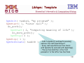
Libhpm: Template
hpmInit( tasked, "my program" );
hpmStart( 1, "outer call" );
do_work();
hpmStart( 2, "computing meaning of life" );
do_more_work();
hpmStop( 2 );
hpmStop( 1 );
hpmTerminate( taskID ); • Calls to hpmInit() and hpmTerminate()
embrace the instrumented part.
• Every instrumentation section starts
with hpmStart() and ends with hpmStop().
• The section identifier is the first
parameter to the latter two functions.
102
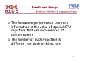
Events and Groups
o The hardware performance counters
information is the value of special CPU
registers that are incremented at
certain events
o The number of such registers is
different for each architecture
103
Registers per Architecture
Processor Architecture
Number of Performance
Counter Registers
Power PC 970
8
POWER4
8
POWER5
8
POWER5+
6
POWER6
6
Blue Gene/L
52
Blue Gene/P
256
104
Counting Registers
o User sees private counter values for the application
o Counting of the special CPU registers is frozen, and
the values are saved whenever the application process
is taken off the CPU and another process is
scheduled
o Counting is resumed when the user application is
scheduled on the CPU
o The special CPU registers can count different events
o There are restrictions on which registers can count
which events
105
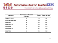
Performance Monitor Counters
Processor
Performance Monitor
Counters
Events Event Groups
PowerPC 970
8
230
49
PowerPC 970 MP
8
230
51
POWER4
8
244
63
POWER4 II
8
244
63
POWER5
6
474
163
POWER5 II
6
483
188
POWER6
6
553
202
106
HPM Metrics
•
•
•
•
•
•
•
•
•
•
•
•
Cycles
Instructions
Floating point instructions
Integer instructions
Load/stores
Cache misses
TLB misses
Branch taken / not taken
Branch mispredictions
Useful derived metrics
– IPC - instructions per
cycle
– Float point rate (Mflip/s)
– Computation intensity
– Instructions per
load/store
– Load/stores per cache
miss
– Cache hit rate
– Loads per load miss
– Stores per store miss
– Loads per TLB miss
– Branches mispredicted %
Derived metrics allow users to correlate the behavior of the application to
one or more of the hardware components
One can define threshold values acceptable for metrics and take actions
107
regarding program optimization when values are below the threshold
Motivation: Message Passing Model
send()
receive()
Task 1
Task 0
Task: a program with local
memory and I/O ports
receive()
Channel: a message queue that
connects two tasks
send()
Task 3
Task 2
Computation
+
Communication
108
MPI Profiler and Tracer
o The MPI profiling and tracing library
collects profiling and tracing data for
MPI programs
Library name
Usage
libmpitrace.a
Library for both the C and
Fortran applications
mpt.h
Header files
109
Compiling and Linking
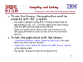
o To use the library, the application must be
compiled with the -g option
– You might consider turning off or having a lower level of
optimization (-O2, -O1,...) for the application when linking
with the MPI profiling and tracing library
– High level optimization affects the correctness of the
debugging information and can also affect the call stack
behavior
o To link the application with the library:
– -L/path/to/libraries, where /path/to/libraries is the path
where the libraries are located
– -lmpitrace, which should be before the MPI library -lmpich,
in the linking order
– The option -llicense to link the license library
110
Compiling on AIX on POWER
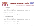
o C example
CC = /usr/lpp/ppe.poe/bin/mpcc_r
TRACE_LIB = -L</path/to/libmpitrace.a> -lmpitrace
mpitrace.ppe: mpi_test.c
$(CC) -g -o $@ $< $(TRACE_LIB) -lm
o Fortran example
FC = /usr/lpp/ppe.poe/bin/mpxlf_r
TRACE_LIB = -L</path/to/libmpitrace.a> -lmpitrace
swim.ppe: swim.f
$(FC) -g -o $@ $< $(TRACELIB)
111
Compiling on Linux on POWER
o C example
CC = /opt/ibmhpc/ppe.poe/bin/mpcc
TRACE_LIB = -L</path/to/libmpitrace.a> -lmpitrace
mpitrace: mpi_test.c
$(CC) -g -o $@ $< $(TRACE_LIB) –lm
o Fortran example
FC = /opt/ibmhpc/ppe.poe/bin/mpfort
TRACE_LIB = -L</path/to/libmpitrace.a> -lmpitrace
statusesf_trace: statusesf.f
$(FC) -g -o $@ $< $(TRACE_LIB)
112
Tracing All Events
o Wrappers can save a record of all MPI
events one after MPI Init(), until the
application completes or until the trace
buffer is full
113
Tracing All Events: Finer Granularity
o Control the time-history measurement within the
application by calling routines to start or stop tracing
o Fortran syntax
call trace_start()
do work + mpi ...
call trace_stop()
o C syntax
void trace_start(void);
void trace_start(void);
trace_start();
do work + mpi ...
trace_stop();
o C++ syntax
extern "C" void trace_start(void);
extern "C" void trace_start(void);
trace_start();
do work + mpi ...
trace_stop();
114
TRACE_ALL_EVENTS disabled
o To use one of the previous control methods,
the TRACE_ALL_EVENTS variable must be
Disabled. Otherwise, it traces all events
o You can use one of the following commands,
depending on your shell, to disable the
variable:
bash
export TRACE_ALL_EVENTS=no
csh
setenv TRACE_ALL_EVENTS no (csh)
115
Environmental Variables
o TRACE_ALL_TASKS
– When saving MPI event records, it is easy
to generate trace files that are too large
to visualize. To reduce the data volume,
when you set TRACE_ALL_EVENTS=yes
o TRACE_MAX_RANK
– To provide more control, you can set
MAX_TRACE_RANK=#
116
Environmental Variables - 2
o TRACEBACK_LEVEL
– In some cases, there might be deeply nested layers on top of MPI and you
might need to profile higher up the call chain (functions in the call stack).
You can do this by setting this environment variable (default value is 0). For
example, setting TRACEBACK_LEVEL=1 indicates that the library must save
addresses starting with the parent in the call chain (level = 1), not with the
location of the MPI call (level = 0)
o SWAP_BYTES
– The event trace file is binary, and therefore, it is sensitive to byte order.
For example, Blue Gene/L is big endian, and your visualization workstation is
probably little endian (for example, x86). The trace files are written in little
endian format by default. If you use a big endian system for graphical
display, such as Apple OS/X, AIX on the System p workstation, and so on),
you can set an environment variable by using one of the following commands
depending on you shell:
bash
export SWAP_BYTES=no
csh
setenv SWAP_BYTES no
Setting this variable results in a trace file in big endian format when you
run your job
117
TRACE_SEND_PATTERN (Blue Gene/L and
Blue Gene/P only)
o
In either profiling or tracing mode, there is an option to collect information about the number of hops for
point-to-point communication on the torus network. This feature can be enabled by setting the
TRACE_SEND_PATTERN environment variable as follows depending on your shell:
bash
export TRACE_SEND_PATTERN=yes
csh
setenv TRACE_SEND_PATTERN yes
o
Wrappers keep track of the number of bytes that are sent to each task, and a binary file send
bytes.matrix is written during MPI Finalize, which lists the number of bytes that were sent from each task
to all other tasks. The binary file has the following format:
D00,D01, ...D0n,D10, ...,Dij , ...,Dnn In this format, the data type Dij is double (in C), and it represents the size of MPI data
that is sent from rank i to rank j. This matrix can be used as input to external utilities that can generate efficient
mappings of MPI tasks onto torus coordinates. The wrappers also provide the average number of hops for all flavors of
MPI Send. The wrappers do not track the message-traffic patterns in collective calls, such as MPI Alltoall. Only point-topoint send operations are tracked. AverageHops for all communications on a given processor is measured as follows:
AverageHops = sum(Hopsi × Bytesi)/sum(Bytesi)
Hopsi is the distance between the processors for MPI communication, and Bytesi is the size
of the data that is transferred in this communication. The logical concept behind this
performance metric is to measure how far each byte has to travel for the communication (in
average). If the communication processor pair is close to each other in the coordinate, the
AverageHops value tends to be small
118
Output: plain text
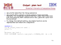
o mpi profile.taskid has the timing summaries
o mpi profile.0 file contains a timing summary from each task.
Currently, for scalability reasons, only four ranks, rank 0 and rank
with (min,med,max) MPI communication time, generate a plain text
file by default
o To change this default setting, one simple function can be
implemented and linked into compilation:
control.c:
int MT_output_trace(int rank) {
return 1;
}
mpitrace: mpi_test.c
$(CC) $(CFLAGS) control.o mpi_test.o $(TRACE_LIB) -lm -o $@
119
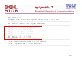
mpi profile.0
mpi profile.0
elapsed time from clock-cycles using freq = 700.0 MHz
----------------------------------------------------------------MPI Routine #calls avg. bytes time(sec)
----------------------------------------------------------------MPI_Comm_size 1 0.0 0.000
MPI_Comm_rank 1 0.0 0.000
MPI_Isend 21 99864.3 0.000
MPI_Irecv 21 99864.3 0.000
MPI_Waitall 21 0.0 0.014
MPI_Barrier 47 0.0 0.000
----------------------------------------------------------------total communication time = 0.015 seconds.
total elapsed time = 4.039 seconds.
-----------------------------------------------------------------
120
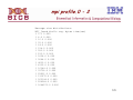
mpi profile.0 - 2
Message size distributions:
MPI_Isend #calls avg. bytes time(sec)
3 2.3 0.000
1 8.0 0.000
1 16.0 0.000
1 32.0 0.000
1 64.0 0.000
1 128.0 0.000
1 256.0 0.000
1 512.0 0.000
1 1024.0 0.000
1 2048.0 0.000
1 4096.0 0.000
1 8192.0 0.000
1 16384.0 0.000
1 32768.0 0.000
1 65536.0 0.000
1 131072.0 0.000
1 262144.0 0.000
1 524288.0 0.000
1 1048576.0 0.000
121
mpi profile.0 - 3
Message size distributions:
MPI_Irecv #calls avg. bytes time(sec)
3 2.3 0.000
1 8.0 0.000
1 16.0 0.000
1 32.0 0.000
1 64.0 0.000
1 128.0 0.000
1 256.0 0.000
1 512.0 0.000
1 1024.0 0.000
1 2048.0 0.000
1 4096.0 0.000
1 8192.0 0.000
1 16384.0 0.000
1 32768.0 0.000
1 65536.0 0.000
1 131072.0 0.000
1 262144.0 0.000
1 524288.0 0.000
1 1048576.0 0.000
----------------------------------------------------------------Communication summary for all tasks:
minimum communication time = 0.015 sec for task 0
median communication time = 4.039 sec for task 20
maximum communication time = 4.039 sec for task 30
122
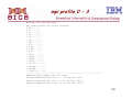
mpi profile.0 - 4
taskid xcoord ycoord zcoord procid total_comm(sec) avg_hops
0 0 0 0 0 0.015 1.00
1 1 0 0 0 4.039 1.00
2 2 0 0 0 4.039 1.00
3 3 0 0 0 4.039 4.00
4 0 1 0 0 4.039 1.00
5 1 1 0 0 4.039 1.00
6 2 1 0 0 4.039 1.00
7 3 1 0 0 4.039 4.00
8 0 2 0 0 4.039 1.00
9 1 2 0 0 4.039 1.00
10 2 2 0 0 4.039 1.00
11 3 2 0 0 4.039 4.00
12 0 3 0 0 4.039 1.00
13 1 3 0 0 4.039 1.00
14 2 3 0 0 4.039 1.00
15 3 3 0 0 4.039 7.00
16 0 0 1 0 4.039 1.00
17 1 0 1 0 4.039 1.00
18 2 0 1 0 4.039 1.00
19 3 0 1 0 4.039 4.00
20 0 1 1 0 4.039 1.00
21 1 1 1 0 4.039 1.00
22 2 1 1 0 4.039 1.00
23 3 1 1 0 4.039 4.00
24 0 2 1 0 4.039 1.00
25 1 2 1 0 4.039 1.00
26 2 2 1 0 4.039 1.00
27 3 2 1 0 4.039 4.00
28 0 3 1 0 4.039 1.00
29 1 3 1 0 4.039 1.00
30 2 3 1 0 4.039 1.00
31 3 3 1 0 4.039 7.00
123
mpi profile.0 - 5
MPI tasks sorted by communication time:
taskid xcoord ycoord zcoord procid total_comm(sec)
avg_hops
0 0 0 0 0 0.015 1.00
9 1 2 0 0 4.039 1.00
26 2 2 1 0 4.039 1.00
10 2 2 0 0 4.039 1.00
2 2 0 0 0 4.039 1.00
1 1 0 0 0 4.039 1.00
17 1 0 1 0 4.039 1.00
5 1 1 0 0 4.039 1.00
23 3 1 1 0 4.039 4.00
4 0 1 0 0 4.039 1.00
29 1 3 1 0 4.039 1.00
21 1 1 1 0 4.039 1.00
15 3 3 0 0 4.039 7.00
19 3 0 1 0 4.039 4.00
31 3 3 1 0 4.039 7.00
20 0 1 1 0 4.039 1.00
6 2 1 0 0 4.039 1.00
7 3 1 0 0 4.039 4.00
8 0 2 0 0 4.039 1.00
3 3 0 0 0 4.039 4.00
16 0 0 1 0 4.039 1.00
11 3 2 0 0 4.039 4.00
13 1 3 0 0 4.039 1.00
14 2 3 0 0 4.039 1.00
24 0 2 1 0 4.039 1.00
27 3 2 1 0 4.039 4.00
22 2 1 1 0 4.039 1.00
25 1 2 1 0 4.039 1.00
28 0 3 1 0 4.039 1.00
12 0 3 0 0 4.039 1.00
18 2 0 1 0 4.039 1.00
30 2 3 1 0 4.039 1.00
124
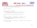
MPI Trace – lab 4
cd /scratch1/cpsosa/bicb8510/c/mpi
module load hpct
silver> make -f make.pi
/opt/ibmhpc/ppe.poe/bin/mpcc -g -o pi pi.c L/opt/ibmhpc/ppe.hpct/lib -lmpitrace –lm
silver> poe ./pi -hfile hostfile -procs 4
20
Enter the number of intervals: (0 quits) pi is
approximately 3.1418009868930938, Error is
0.0002083333033007
0
Enter the number of intervals: (0 quits) wrote trace file:
single_trace
125
Appendix I: Xprofiler Options
126
Xprofiler Options - 1
o -b Xprofiler -b a.out gmon.out
– This option suppresses the printing of the field descriptions for the
Flat Profile, Call Graph Profile, and Function Index reports when
they are written to a file with the Save As option of the File menu
o -s Xprofiler -s a.out gmon.out.1 gmon.out.2 gmon.out.3
– If multiple gmon.out files are specified when Xprofiler is started,
this option produces the gmon.sum profile data file. The gmon.sum
file represents the sum of the profile information in all the
specified profile files. Note that if you specify a single gmon.out
file, the gmon.sum file contains the same data as the gmon.out file
o -z Xprofiler -z a.out gmon.out
– This option includes functions that have both zero CPU usage and no
call counts in the Flat Profile, Call Graph Profile, and Function Index
reports. A function will not have a call count if the file that contains
its definition was not compiled with the -pg option, which is common
with system library files
127
Xprofiler Options - 2
o -a Xprofiler –a pathA:@:pathB
–
This option adds alternative paths to search for source code and library files, or
changes the current path search order. When using this command line option, you can
use the at sign (@) to represent the default file path, in order to specify that other
paths be searched before the default path
o -c Xprofiler a.out gmon.out –c config_file_name
–
This option loads the specified configuration file. If the -c option is used on the
command line, the configuration file name specified with it is displayed in the
Configuration File (-c): text field, in the Loads Files window, and the Selection field of
the Load Configuration File window. When both the -c and -disp_max options are
specified on the command line, the -disp_max option is ignored. However, the value that
was specified with it is displayed in the Initial Display (-disp_max): field in the Load
Files window the next time it is opened
o -disp_max Xprofiler -disp_max 50 a.out gmon.out
–
This option sets the number of function boxes that Xprofiler initially displays in the
function call tree. The value that is supplied with this flag can be any integer between 0
and 5,000. Xprofiler displays the function boxes for the most CPU-intensive functions
through the number that you specify. For instance, if you specify 50, Xprofiler displays
the function boxes for the 50 functions in your program that consume the most CPU.
After this, you can change the number of function boxes that are displayed via the
Filter menu options. This flag has no effect on the content of any of the Xprofiler
reports
128
Xprofiler Options - 3
o -e Xprofiler -e function1 -e function2 a.out gmon.out
– This option de-emphasizes the general appearance of the function
box or boxes for the specified function or functions in the function
call tree. This option also limits the number of entries for these
function in the Call Graph Profile report. This also applies to the
specified function’s descendants, as long as they have not been
called by non-specified functions. In the function call tree, the
function box or boxes for the specified function or functions
appears to be unavailable. Its size and the content of the label
remain the same. This also applies to descendant functions, as long
as they have not been called by non-specified functions. In the Call
Graph Profile report, an entry for the specified function only
appears where it is a child of another function or as a parent of a
function that also has at least one non-specified function as its
parent. The information for this entry remains unchanged. Entries
for descendants of the specified function do not appear unless they
have been called by at least one non-specified function in the
program.
129
Xprofiler Options - 4
o
-E Xprofiler -E function1 -E function2 a.out gmon.out
–
This option changes the general appearance and label information of the function box
or boxes for the specified function or functions in the function call tree. In addition,
this option limits the number of entries for these functions in the Call Graph Profile
report and changes the CPU data that is associated with them. These results also apply
to the specified function’s descendants, as long as they have not been called by nonspecified functions in the program. In the function call tree, the function box for the
specified function appears to be unavailable, and its size and shape also change so that
it appears as a square of the smallest allowable size. In addition, the CPU time shown in
the function box label appears as zero. The same applies to function boxes for
descendant functions, as long as they have not been called by non-specified functions.
This option also causes the CPU time spent by the specified function to be deducted
from the left side CPU total in the label of the function box for each of the specified
ancestors of the function. In the Call Graph Profile report, an entry for the specified
function only appears where it is a child of another function or as a parent of a function
that also has at least one non-specified function as its parent. When this is the case,
the time in the self and descendants columns for this entry is set to zero. In addition,
the amount of time that was in the descendants column for the specified function is
subtracted from the time listed under the descendants column for the profiled
function. As a result, be aware that the value listed in the % time column for most
profiled functions in this report will change.
130
Xprofiler Options - 5
o -f Xprofiler -f function1 -f function2 a.out gmon.out
– This option de-emphasizes the general appearance of all function
boxes in the function call tree, except for that of the specified
function or functions and its descendant or descendants. In
addition, the number of entries in the Call Graph Profile report for
the non-specified functions and non-descendant functions is limited.
The -f flag overrides the -e flag. In the function call tree, all
function boxes, except for that of the specified function or
functions and its descendant or descendants, appear to be
unavailable. The size of these boxes and the content of their labels
remain the same. For the specified function or functions, and its
descendant or descendants, the appearance of the function boxes
and labels remains the same. In the Call Graph Profile report, an
entry for a non-specified or non-descendant function only appears
where it is a parent or child of a specified function or one of its
descendants. All information for this entry remains the same.
131
Xprofiler Options - 6
o -F Xprofiler -F function1 -F function2 a.out gmon.out
– This option changes the general appearance and label information of all
function boxes in the function call tree, except for that of the specified
function or functions and its descendants. In addition, the number of entries
in the Call Graph Profile report for the non-specified and non-descendant
functions is limited, and the CPU data associated with them is changed. The
-F flag overrides the -E flag. In the function call tree, all function boxes,
except for that of the specified function or functions and its descendant or
descendants, appear to be unavailable. The size and shape of these boxes
change so that they are displayed as squares of the smallest allowable size.
In addition, the CPU time shown in the function box label appears as zero.
In the Call Graph Profile report, an entry for a non-specified or nondescendant function only is displayed where it is a parent or child of a
specified function or one of its descendants. When this is the case, the time
in the self and descendants columns for this entry is set to zero. As a
result, be aware that the value listed in the % time column for most profiled
functions in this report will change
o -L Xprofiler –L /lib/profiled
– This option sets the path name for locating shared libraries. If you plan to
specify multiple paths, use the Set File Search Paths option of the File menu
on the Xprofiler GUI
132
Appendix II: Computer
Performance
Name
FLOPS
yottaFLOPS
1024
zettaFLOPS
1021
exaFLOPS
1018
petaFLOPS
1015
teraFLOPS
1012
gigaFLOPS
109
megaFLOPS
106
kiloFLOPS
103
http://en.wikipedia.org/wiki/FLOPS
133
Outline
o
Part I: Hardware
–
–
–
o
Historical perspective: Why do we need MPPs?
Overview of massively parallel processing (MPP)
Architecture
Part II: Software
–
–
–
–
Overview
Compilers
MPI
Building and Running Examples on Blue Gene
•
o
Part III: Applications
–
–
–
MPP architecture and its impact on applications
Performance tools
Introduction to code optimization
•
–
–
–
–
–
Hands-n session 2
Mapping applications on a massively parallel architecture
Applications landscape
Challenges and characteristics of Life Sciences applications
Selected Bioinformatics applications
Selected Structural Biology applications
•
o
o
Hands-on session 1
Hands-on session 3
Summary
Biomedical Informatics & Computational Biology
134
Scientific and Engineering Applications Landscape
Rational
Drug Design
Petroleum
Reservoir
Molecular
Dynamics
Reaction
Diffusion
Fracture
Mechanics
Materials
Sciences
Semiconductors
Nanotechnology
Stochastic
Process
VLSI
Design
Elementary
Flow
Fourier
Methods
N-Body
Discrete
Events
Monte
Carlo
Graph
Theory
Partial Diff.
Equations
Scientific and Engineering
Applications Landscape
Pattern
Matching
Bioinformatics
Data
Mining
Fluid
Dynamics
Flows in Porous
Media
Molecular
Modeling
Network
Flow
Multiphase
Flow
Genome
Computing
Symbolic
Processing
Structural
Mechanics
Transport
Graphics
Structural
Display
Ord. Diff.
Equations
Seismic
Processing
Fields
Cryptography
Proteomics
Weather and
Climate
Aerodynamics
Particle
Physics
135
MPP Challenges for
Applications Developers
o MPP flops are not only dependent on the individual
performance of the CPU
o Performance on the holistic system
– Memory system
– File access
– Network (messaging)
– This type of system is not appropriate for every
application
• It is harder to take advantage of all processors
o Applications that can take advantage of large number of
processors need access to larger systems
136
Mapping Applications
New Hardware
Architectures
Applications
Enablement?
Develop New
Software Package
Multidisciplinary
Team
Port and Optimize
Existing Application
Collaboration/
Developers 137
Classical Molecular Dynamics
CHARACTERISTICS
These models were developed to
describe molecular structures and
properties in as practical a manner as
possible for very large systems mainly
of biological interest
CHALLENGE
o Micro-seconds scale simulations require an order of 103
increases in the computing power of contemporary high-end
systems
o Improving code performance and scalability for longer time
and length scales simulations
o Novel algorithms:
– To reduce the performance and scaling bottlenecks
– To minimize memory requirements for large systems
USAGE
o Protein modeling: structure, folding, dynamics and function
o Compute-intensive applications
138
Ligand-Protein Interactions
CHARACTERISTICS
Molecular docking is used in structure-based
drug design. The computational aspects can
be divided into two parts. Ligand atoms
being located inside the cavity or binding
pocket of a receptor, which is a large
biomolecule and scoring or identifying
the most favorable interactions
CHALLENGE
o Improving code performance and scalability for virtual
screening of millions of ligands
USAGE
o
Drug Discovery
o
Compute-intensive applications
139
Bioinformatics
Output
Database
Query
SWISSPROT
CHARACTERISTICS
o Science necessary to manage, process, and understand large
amounts of data, for instance from the sequencing of the human
genome, or from large databases containing information about
plants and animals
CHALLENGE
o Database fragmentation and distribution
o Parallelization of very large databases versus very large queries
USAGE
o Database searches; homology
o Data-intensive applications
140
Quantum Chemistry
ΗΨ = ΕΨ
CHARACTERISTICS
o These methods have traditionally been used for computing very
accurate properties of small molecules to
o Complex systems with 1000s of atoms
CHALLENGE
o
o
Parallel scalability to large number of processors
Parallelization of Linear Algebra based-algorithms
USAGE
o Small to medium molecules properties
o Compute-intensive applications
141
Bioinformatics: Areas of Interest
SEQUENCE ANALYSIS AND
ALIGNMENT
COMPARATIVE GENOMICS
EVOLUTION AND
PHYLOGENY
GENE REGULATION AND
TRANSCRIPTOMICS
PROTEIN STRUCTURE AND
FUNCTION
PROTEIN INTERACTIONS
AND MOLECULAR
NETWORKS
TEXT MINING
DATABASES AND
ONTOLOGIES
OTHER BIOINFORMATICS
APPLICATIONS AND
METHODS
BIOINFORMATICS OF
DISEASE
142
Source: ISMB 2008, Toronto Canada
Bioinformatics: Selected Applications
– HMMER
– mpiBLAST-PIO
– PBPI
143
HMMER
o Hidden Markov models (HMMs) were initially
introduced for pattern recognition in digitized
acoustics of the human voice
Oystein Thorsen,
Michigan Technological U
BLAST
Karl Jiang
U of Miami
HMMER
http://hmmer.janelia.org/
– L. R. Rabiner, “A Tutorial on Hidden Markov
Models and Selected Applications in Speech
Recognition”, Proceedings of the IEEE, Vol.
77, 257-286, 1989
– A. Krogh, M. Brown, I. S. Mian, K. Sjolander,
K and Haussler, D. (1994). “Hidden Markov
models in computational biology:
Applications to protein modeling” J. Mol.
Biol., vol. pp. 1501–1531
– S.R. Eddy, “Multiple Alignment Using Hidden
Markov Models,” Proc. Third Int’l Conf.
Intelligent Systems Molecular Biology
(ISMB ’95), vol. 3, pp. 114-120, 1995.
144
Hidden Markov Models in Bioinformatics
• The UC Santa Cruz profile HMM software(SAM), probably the closest
relative of HMMER
• Philipp Bucher's PFTOOLS package implements "generalized profiles",
which are substantially similar to profile HMMs
• The commercial HMMpro package from Pierre Baldi and Yves Chauvin
at NetID, Inc. implements more general HMM architectures than just
profile HMMs, and also comes with a nifty Java display
• Andy Neuwald's PROBE software implements models based on multiple
ungapped HMM motifs, and includes an implementation of training
models by Gibbs sampling
• The UC San Diego META-MEME package from Michael Gribskov, Bill
Grundy, Tim Bailey, and others implements multiple ungapped HMM
motif models, similar to PROBE
• NCBI's PSI-BLAST server implements a stripped down but ultra-fast
version of iterative profile HMM searches. This is a convenient Web
server for folks who don't want to hassle with installing software
locally
• Ewan Birney's WISETOOLS package can take a HMMER model and
search it against EST or genomic DNA sequence, doing six-frame
145
translation and allowing for frameshifts and introns
Hidden Markov Models References
o Several software packages are currently available:
HMMER http://hmmer.janelia.org/
SAM http://www.cse.ucsc.edu/research/compbio/sam.html
PFTOOLS http://www.isrec.isb-sib.ch/profile/profile.html
HMMpro http://www.bio.net/hypermail/bio-software/1999January/020107.html
– GENEWISE http://www.ebi.ac.uk/Wise2/
– META-MEME http://metameme.sdsc.edu/
– PSI-BLAST http://blast.ncbi.nlm.nih.gov/Blast.cgi
–
–
–
–
146
HMMs and Applications
o HMM:
– Profile HMMs are statistical models of multiple sequence
alignments
• Capture position-specific information on how conserved
each column of the alignment is, and which residues are
likely
o Applications:
– Evolutionary homology in family of proteins
– Automated annotation of the domain structure of proteins
– Automated construction and maintenance of large multiple
alignment databases
Source: HMMER’s User Guide 2.3.2
147
HMMER 2.3.2
o hmmalign Align sequences to an existing model
o hmmbuild Build a model from a multiple sequence alignment
o hmmcalibrate Takes an HMMand empirically determines parameters
that are used to make searches more sensitive, by calculating more
accurate expectation value scores (E-values)
o hmmconvert Convert a model file into different formats, including a
compact HMMER 2 binary format, and “best effort” emulation of GCG
profiles
o hmmemit Emit sequences probabilistically from a profile HMM
o hmmfetch Get a single model from an HMM database
o hmmindex Index an HMM database
o hmmpfam Search an HMM database for matches to a query sequence
o hmmsearch Search a sequence database for matches to an HMM
S.R. Eddy HMMER User’s Guide: Biological Sequence Analysis Using Profile Hidden Markov Models, Version 2.3.2, http://
hmmer.wustl.edu/, Oct. 1998
148
HMMER 2.3.2 Parallel Modules
o Three have been parallelized:
– hmmcalibrate: Takes an HMM and empirically
determines parameters that are used to make
searches more sensitive, by calculating more
accurate expectation value scores (E-values)
– hmmpfam: is used to search a profile HMM
database to a sequence query
– hmmsearch: is used to carry out sequence
database searches to match an HMM
S.R. Eddy HMMER User’s Guide: Biological Sequence Analysis Using Profile Hidden Markov Models, Version 2.3.2, http://
hmmer.wustl.edu/, Oct. 1998
149
Single Node Optimization: Data Set
o Queries:
– The two queries consisted of gi|1174687|sp|p42461|THIX_CORGL
Thiamine biosynthesis protein X and 50 aligned globin sequences as
provided in the HMMER version 2.2 (globins50)
– The first query corresponds to a single sequence of a small protein
with 135 characters (amino acids)
o Databases :
– Small protein database SWISS-PROT; 49787460 characters or
108891 sequences.
– The second database NR; 459219939 characters 929420 sequences
– This second database is larger than the first one by almost a factor
of 10
150
Profiler Partial Output
index
%time
self descendents
2.57
765.52
[1]
89.4
2.57
765.52
714.02
13.71
0.06
15.49
4.94
5.10
.TraceScoreCorrection [9]
3.61
5.48
0.17
1.45
0.01
0.65
.PostprocessSignificantHit [41]
0.24
0.00
0.22
0.00
0.03
0.15
0.06
0.04
[65]
0.05
0.00
.pthread_mutex_lock [78]
0.01
0.00
.pthread_mutex_unlock [96]
0.00
0.00
[137]
called/total
parents
called+self
name
index
called/total
children
1/1
1
727771/727771
727772/727772
727771/749381
._pthread_body [2]
.@2@worker_thread [1]
.P7Viterbi [3]
.ReadSeq [5]
230545997/230546004
4366626/13380941
3720/3720
2183313/36337220
2117717/2214013
727771/13380947
727771/727771
.toupper [12]
.free [15]
.log [17]
.exp [54]
.malloc [20]
.AddToHistogram
1455543/1455545
1455543/1455545
1/1
.pthread_exit
151
Selected Techniques
o Maximize Expressions
– Transforming if-max calculation into using
the ?: operator
o Use of registers
– Using registers to carry values to next
iterations, eliminating a large number of
load operations
o Fusion
– Helped increase registers reuse
o Better arrays access
152
Maximizing Expressions
for (k = 1; …
{
.
.
.
if ((sc = dmx[i-1][k-1]…
.
.
.
After maximizing expressions
for (k = 1; …
{
.
.
.
sc4 = dmx[i-1][k-1] …
sc5 = (sc2 > sc1) ? sc2:sc1;
sc6 = (sc4 > sc3) ? sc4 : sc3;
sc7 = (sc6 > sc5) ? sc6 : sc5;
.
.
.
153
hmmsearch Timings with a Single
Query and the NR Database
14000
POWER3 375 MHz
POWER4 1.3 GHz
12000
10000
8000
6000
3.55x
4000
2.40x
2000
0
Original
Optimized
154
Massively Parallel Version
I. Single node optimization
II. Port from PVM → MPI
III. BG parallel optimizations
K Jiang, O Thorsen, A Peters, B Smith and C. P. Sosa, An Efficient Parallel Implementation of the Hidden Markov
Methods for Genomic Sequence Search on a Massively Parallel SystemIEEE TRANSACTIONS ON PARALLEL AND
DISTRIBUTED SYSTEMS, VOL. 19, NO. 1, JANUARY 2008
155
PVM → MPI
– PVM calls
pvm_initsend
pvm_pk (pack) instructions or pvm_upk (unpack)
pvm_send or pvm_recv
– Replaced with MPI calls
MPI_Send for each pvm_send
MPI_Recv for every pvm_recv
memcpy for every pvm_pk and pvm_upk
MPI_Send and MPI_Recv to send and receive the entire
package
• Functions were constructed to pack the HMM data
along with other control structures in parallel with the
PVM to MPI conversions
K Jiang, O Thorsen, A Peters, B Smith and C. P. Sosa, An Efficient Parallel Implementation of the Hidden Markov Methods
for Genomic Sequence Search on a Massively Parallel SystemIEEE TRANSACTIONS ON PARALLEL AND
DISTRIBUTED SYSTEMS, VOL. 19, NO. 1, JANUARY 2008
156
hmmsearch Parallel
Scheme
Image source: K Jiang, O Thorsen, A Peters, B Smith and C. P. Sosa, An Efficient Parallel Implementation of the Hidden
Markov Methods for Genomic Sequence Search on a Massively Parallel SystemIEEE TRANSACTIONS ON PARALLEL
AND DISTRIBUTED SYSTEMS, VOL. 19, NO. 1, JANUARY 2008
157
hmmseacrh Plain MPI Port
Normalized search time
1.2
1
0.8
0.6
Plain
0.4
0.2
0
32
64
128
256
512
1024
Processors
158
Blue Gene Optimizations
– Alternate Sequence File Indexing
• Open file and skip to offset
– Multiple-Master Configuration
• Single master not enough to handle communication
• Use current infrastructure and include another
management level
• Multiple-master structure is able to do an intermediate
processing step
– Dynamic Data Collection
• Eliminate gather operation
• Introduce buffer and tolerance (threshold)
– Database Caching in hmmpfam
• Eliminate excessive I/O
– Load balancing
• Index file and offset
K Jiang, O Thorsen, A Peters, B Smith and C. P. Sosa, An Efficient Parallel Implementation of the Hidden Markov
Methods for Genomic Sequence Search on a Massively Parallel SystemIEEE TRANSACTIONS ON PARALLEL AND
DISTRIBUTED SYSTEMS, VOL. 19, NO. 1, JANUARY 2008
159
Master-Supermaster Scheme
Image source: K Jiang, O Thorsen, A Peters, B Smith and C. P. Sosa, An Efficient Parallel Implementation of the Hidden
Markov Methods for Genomic Sequence Search on a Massively Parallel SystemIEEE TRANSACTIONS ON PARALLEL
AND DISTRIBUTED SYSTEMS, VOL. 19, NO. 1, JANUARY 2008
160
hmmcalibrate
12000
Time (sec)
10000
8000
6000
4000
2000
0
32
64
128
256
512 1024 2048
Processors
Parallel performance using the first 327 entries of the
Pfam database
K Jiang, O Thorsen, A Peters, B Smith and C. P. Sosa, An Efficient Parallel Implementation of the Hidden Markov
Methods for Genomic Sequence Search on a Massively Parallel SystemIEEE TRANSACTIONS ON PARALLEL AND
DISTRIBUTED SYSTEMS, VOL. 19, NO. 1, JANUARY 2008
161
hmmseacrh
HMMSearch parallel optimizations
1.2
Normalized search time
1
0.8
0.6
0.4
0.2
0
32
64
128
256
Processors
512 1024
hmmsearch parallel
performance using 50
proteins of the globin
family
For each processor
Plain
count, the left bar
shows the original
Multiple master
PVM to MPI port
The second bar
With dynamic data
shows the multiple
collection
master
Load Balanced
implementation.
The third bar shows
the dynamic data
collection
implementation
the right bar shows
the load balancing
implementation
K Jiang, O Thorsen, A Peters, B Smith and C. P. Sosa, An Efficient Parallel Implementation of the Hidden Markov
Methods for Genomic Sequence Search on a Massively Parallel SystemIEEE TRANSACTIONS ON PARALLEL AND
DISTRIBUTED SYSTEMS, VOL. 19, NO. 1, JANUARY 2008
162
hmmpfam
1000
S peedu p
800
600
Optimized
Linear
400
200
0
0
200
400
600
Processors
800
1000
o Opposite of
hmmsearch, but
similar in program
structure (same
optimizations)
o In addition to the
other
optimizations, data
caching allowed
fast processing of
thousands of query
sequences
o Also scales close to
linearly up to 1000+
nodes
K Jiang, O Thorsen, A Peters, B Smith and C. P. Sosa, An Efficient Parallel Implementation of the Hidden Markov
Methods for Genomic Sequence Search on a Massively Parallel SystemIEEE TRANSACTIONS ON PARALLEL AND
DISTRIBUTED SYSTEMS, VOL. 19, NO. 1, JANUARY 2008
163
hmmsearch Performance
Improvements on BG/P
700
Viterbi Default
600
Viterbi Optimized
Time in Sec.
500
400
300
200
100
0
32
64
128
256
512
o HMM profile: globins
o UniProt Database:
~2.9 million sequences
o Jobs were submitted
using LoadLeveler to
Blue Gene/P
o 20-25% performance
improvement
1024
Processors
164
BLAST
Output
Database
Query
SWISSPROT
o BLAST®: Basic Local Alignment Search Tool
– A set of similarity-search programs for searching available
sequence databases (regardless of whether the query is protein
or DNA)
– The most popular tool in bioinformatics
• NCBI BLAST server: ~ 500,000 query submissions per day
165
What is the Problem?
Database size
increasing faster
than our ability to
compute on it
Hexokinase, from the yeast species Saccharomyces cerevisiae
5
10
15
20
25
30
1 AASX DXS L VEVH XXVF I VPPX IL Q AVVS IA
31 T T R X D D X D S A A A S I P M V P G W V L K Q V X G S Q A
61 G S F L A I V M G G G D L E V I L I X L A G Y Q E S S I X A
91 S R S L A A S M X T T A I P S D L W G N X A X S N A A F S S
121 X E F S S X A G S V P L G F T F X E A G A K E X V I K G Q I
151 T X Q A X A F S L A X L X K L I S A M X N A X F P A G D X X
181 X X V A D I X D S H G I L X X V N Y T D A X I K M G I I F G
211 S G V N A A Y W C D S T X I A D A A D A G X X G G A G X M X
241 V C C X Q D S F R K A F P S L P Q I X Y X X T L N X X S P X
271 A X K T F E K N S X A K N X G Q S L R D V L M X Y K X X G Q
301 X H X X X A X D F X A A N V E N S S Y P A K I Q K L P H F D
331 L R X X X D L F X G D Q G I A X K T X M K X V V R R X L F L
361 I A A Y A F R L V V C X I X A I C Q K K G Y S S G H I A A X
391 G S X R D Y S G F S X N S A T X N X N I Y G W P Q S A X X S
421 K P I X I T P A I D G E G A A X X V I X S I A S S Q X X X A
451 X X S A X X A
Output
Query
Database
SWISSPROT
166
Levels of Parallelism and Potential I/O
Bottlenecks
Fine Grained
Medium Grained Coarse Grained
Subject(s)
One Sequence
One Sequence
N Sequences
Target(s)
One Sequence
M Sequences
(in database)
M Sequences
(in database)
Parallelism
Multiple
Alignments on
Single Sequence
Pairs
Partition
Database
[Multiple
targets
searched at
once]
Replicate
Database
[Partition Input
Sets]
I/O Bottlenecks
R.C. Braun, K. T. Pedretti, T.L. Casavant, T.E. Scheetz, C.L. Birkett, C.A. Roberts, Three
Complementary Approaches to Parallelization of Local BLAST Service on Workstation Clusters, Future
167
Generation Computer Systems, 17, 745(2001).
BLAST to mpiBLAST-PIO Evolution
o mpiBLAST
– DB is partitioned and BLAST is executed in
parallel
o pioBLAST
– Uses parallel I/O to improve mpiBLAST
– Dynamic (virtual) DB partitioning
– Improved result merging
o mpiBLAST-pio
– Incorporates the parallel-I/O performance
enhancements of pioBLAST into mpiBLAST
o
A. Darling, L. Carey, and W. Feng. The design, implementation, and
evaluation of mpiBLAST. In Proceedings of the ClusterWorld
BLAST
mpiBLAST
pioBLAST
Conference and Expo, in conjunction with the 4th International
Conference on Linux Clusters: The HPC Revolution, 2003.
o
o
H. Rangwala, E. Lantz, R. Musselman, K. Pinnow, B. Smith, , and B.
Wallenfelt. Massively Parallel BLAST for the Blue Gene/L. In High
Availability and Performance Workshop, 2005.
C. Oehmen and J. Nieplocha. Scalablast: A scalable implementation of
blast for high-performance data-intensive bioinformatics analysis.
IEEE Trans. Parallel Distrib. Syst., 17(8), 2006
mpiBLAST-pio
168
Importance of mpiBLAST-PIO
http://www.mpiblast.org/
o Completion of the sequencing of human genome
o New organisms being sequenced at a rapid rate
– NCBI BLAST server: ~ 500,000 query submissions per day
– Queries per day doubling approximately every year
o Trend in GenBank Database
– Doubling in size every year.
– Consequence: Database size
increasing faster than our ability to
compute on it.
o What to Do?
– Faster & more scalable parallel
algorithms, i.e., mpiBLAST-PIO.
– More efficient use of state-ofthe-art hardware, i.e., BG/L and
BG/P.
169
http://www.ncbi.nlm.nih.gov/Genbank/genbankstats.html
Initial Problems
Query (28k)
o Disk I/O overload
o Master overworked
DB (2.4M)
Master
1
2
Worker
3
H. Lin, X. Ma, P. Chandramohan, A. Geist, and N. Samatova. Efficient data access for parallel BLAST. In
IPDPS 2005 Proceedings of the 19th IEEE International Parallel and Distributed Processing Symposium.
170
Storing Files in Memory
o Original BLAST version utilizes mmap to store the
database in memory
o mmap is not implemented as a part of the Blue Gene/L
operating system
o With all nodes sharing the same file system, I/O
contention severely limits the scaling of this
application
o Solution: “virtual file manager” (VFM)
Oystein Thorsen, Karl Jiang, Amanda Peters, Brian Smith, Heshan Lin, Wu-chun Feng, Carlos P. Sosa, "Parallel Genomic SequenceSearch on a Massively Parallel System", Conference On Computing Frontiers Proceedings of the 4th international conference on
Computing frontiers, Ischia, Italy, 59 - 68 (2007)
171
Virtual File Manager
o VFM is used to store:
– database fragments in memory
– query files in memory
– various temporary files in memory
o Eliminates disk I/O
o Allows files distribution using MPI when workers
need the same file
Oystein Thorsen, Karl Jiang, Amanda Peters, Brian Smith, Heshan Lin, Wu-chun Feng, Carlos P. Sosa, "Parallel Genomic SequenceSearch on a Massively Parallel System", Conference On Computing Frontiers Proceedings of the 4th international conference
172on
Computing frontiers, Ischia, Italy, 59 - 68 (2007)
Multiple Masters
o Second level of management
–Limit the number of workers for a single
master
o Groups of nodes
–One master for each group working on
separate query sequences
Oystein Thorsen, Karl Jiang, Amanda Peters, Brian Smith, Heshan Lin, Wu-chun Feng, Carlos P. Sosa, "Parallel
173
Genomic Sequence-Search on a Massively Parallel System", Conference On Computing Frontiers Proceedings
of the 4th international conference on Computing frontiers, Ischia, Italy, 59 - 68 (2007)
Divide into Groups
Query (28k)
DB (2.4M)
Super-master
Master
Worker
Oystein Thorsen, Karl Jiang, Amanda Peters, Brian Smith, Heshan Lin, Wu-chun Feng, Carlos P. Sosa, "Parallel
174
Genomic Sequence-Search on a Massively Parallel System", Conference On Computing Frontiers Proceedings
of the 4th international conference on Computing frontiers, Ischia, Italy, 59 - 68 (2007)
Divide into Groups
Query (28k)
oQuery fragmentation
DB (2.4M)
–Load-balancing
Super-master
Master
Worker
oMultiple output
1
2
3
175
Oystein Thorsen, Karl Jiang, Amanda Peters, Brian Smith, Heshan Lin, Wu-chun Feng, Carlos P. Sosa, "Parallel Genomic SequenceSearch on a Massively Parallel System", Conference On Computing Frontiers Proceedings of the 4th international conference on
Computing frontiers, Ischia, Italy, 59 - 68 (2007)
Fragment Distribution
176
The “DNA” of mpiBLAST-PIO on BG
o Approach
– Exploit the distributed processing power and memory of
supercomputing systems, particularly for large datasets.
o Software Environment
– Operating System: Linux
– Programming Language: C++ and MPI (Message Passing Interface)
o Overview of Parallel Algorithm
– Segment query file into individual queries (only one query shown
below)
– Fragment database and distribute to the worker nodes.
177
mpiBLAST-PIO 1.4 Performance on BG/L
8192
Performance Scaling
7168
Parallel Speedup
6144
5120
4096
3072
2048
1024
0
0
1024 2048 3072 4096 5120 6144 7168 8192
• Thick Line
• Ideal Speed-Up
• Thin Solid Line
• Speed-up for a large
query against nr
• Dashed Line
• Speed-up for a medium
query against nr
• Dotted Line
• Speed-up for small query
against nr
Nodes in co-processor mode
Oystein Thorsen, Karl Jiang, Amanda Peters, Brian Smith, Heshan Lin, Wu-chun Feng, Carlos P. Sosa, "Parallel
178
Genomic Sequence-Search on a Massively Parallel System", Conference On Computing Frontiers Proceedings
of the 4th international conference on Computing frontiers, Ischia, Italy, 59 - 68 (2007)
mpiBLAST 1.5 Performance Improvements
Partition i
o DB frags cached in workers, queries
streamed across
o One output file per partition
o Results merged and written to GPFS
through I/O nodes
Image source:sH. Lin, et al.
Partition 1
Partition 2
qi
qi
qi+1
…
qi
qi+1
qi+1
qi+2
qi+2
Partition i
qi+2
Compute Nodes
Compute Nodes
Compute Nodes
IO Node
IO Node
IO Node
G P F S
File 1
qi
File 2
…
…
Config example
Fileqii+1
Disk
Disk
Disk
Disk
Disk
PSize 128
4 DBs / partition
32768/128179
= 256
179
partitions
Compare I/O Strategies – Single Partition
o Experimental setup
– Database: NT (over 6 million seqs, 23 GB raw size)
– Query: 512 sequences randomly sampled from the database
– Metric: Overall execution time
WM outperforms WC
and WI by a factor
of 2.7 and 4.9
180
Images source: H. Lin SC’’08
Performance of Latest Research
Prototype on Blue Gene/P
o Self comparison of Microbial Gnome database (5.2
GB raw size, 16 million sequences)
36864
32768
Linear
mpiBLAST-PIO
Parallel Speedup
28672
24576
20480
16384
12288
8192
4096
0
0
4096 8192 12288 16384 20480 24576 28672 32768 36864
Number of Cores (VN mode)
o Scalability tests
–Search a quarter million of
randomly sampled sequences
against the database itself
–Achieve 93% parallel
efficiency on 32768 cores (8rack BG/P)
o Complete genome-to-genome
comparison
–Finish searching 16 million
vs. 16 million sequences within
12 hours
H. Lin, P. Balaji, R. Poole, C. P. Sosa, X. Ma and W. Feng, “Massively Parallel Genomic Sequence Search on the Blue
181
Gene/P Architecture,” IEEE/ACM International Conference for High-Performance Computing, Networking, Storage
and Analysis (SC), 2008
What is PBPI?
o PBPI is an open source implementation of Parallel
Bayesian Phylogenetic Inference
o Combines sequential optimization and parallel
processing to reduce execution times
o Supports large problem sizes
182
PBPI: http://www.pbpi.org/
PBPI uses MPI (message passing interface) and runs under
Linux. Its parallel algorithm can be summarized as:
(1) Multi-dimensional data and task distribution across
multi-dimensional grid topology organization of
processors;
(2) Context aware synchronization across the whole grid
and sub grid.
PBPI significantly reduces phylogenetic inference time by
exploiting distributed processing power and memory,
especially for large data set. For proper sizes of
phylogenetic problem, PBPI is capable to scale up to
thousands of processors on Blue Gene
183
Scalability on BG/L
Relative Speedup
256
512
1024
2048
4096
18
16
14
12
10
8
6
4
2
0
32 chains
64 chains
X. Feng, D. A. Buell, J. R. Rose and P. J. Waddell. "Parallel algorithms for Bayesian phylogenetic inference,"
Journal of Parallel and Distributed Computing (JPDC), Volume 63, Issues 7-8, 2003.
X. Feng, K.W. Cameron and D. A. Buell. "PBPI: a high performance Implementation of Bayesian Phylogenetic
Inference," ACM/IEEE SC 2006: the International Conference on High Performance Computing,
Networking, Storage and Analysis, November 2006, Tampa, FL
X. Feng, K.W. Cameron, B. Smith, and C. Sosa. "Building the Tree of Life on Tera-scale Systems," the 21st
International Parallel and Distributed Processing Symposium (IPDPS 07), April 2007, Long Beach, CA. 184
Molecular Docking &
Virtual Screening
o Ligand-receptor docking
Source: http://www.cs.princeton.edu/courses/archive/fall07/cos597A/index.html
185
Energetics and Conformation
E
Conformational Coordinates
Source: http://www.cs.princeton.edu/courses/archive/fall07/cos597A/index.html
186
DOCK6
o
o
o
o
DOCK 5: D Moustakas and P T Lang, et
al. J Comput Aided Mol Des (2006)
20:601–619
DOCK 5: D Moustakas, S C H Pegg, and
I D Kuntz in Virtual Screening in Drug
Discovery, Edited by J. Alvarez and B.
Shoichet, Taylor&Francis, Inc.
DOCK 6: P T Lang PT et al. (in
preparation)
MPP DOCK: A Peters, M E. Lundberg, C P
Sosa, and P. Therese Lang: . High
Throughput Computing Validation for
Drug Discovery Using the DOCK Program
on a Massively Parallel System, REDP4410-00 Redpapers, published 16 April
2008
187
Embarrassingly Parallel
Create database of potential drug candidates
For each independent node, load:
DOCK binary
Receptor input files
Subset of potential drug candidates
Store docking score results into database
188
Multi-level Parallelization of AutoDock 4.2
Andrew P Norgan1, Paul S Coffman2, Jean-Pierre Kocher1,
David J. Katzmann1, Carlos P. Sosa2,3
1Mayo Clinic, 2IBM Corporation, Rochester, MN,
3Biomedical Informatics and Computational Biology, UMR
Andrew P Norgan1, Paul S Coffman, Jean, Pierre Kocher, David J. Katzmann,
Carlos P. Sosa, BICB Research Symposium, University of Minnesota Rochester,
June 25, 2010, Rochester, MN
189
Outline
o
Part I: Hardware
–
–
–
o
Historical perspective: Why do we need MPPs?
Overview of massively parallel processing (MPP)
Architecture
Part II: Software
–
–
–
–
Overview
Compilers
MPI
Building and Running Examples on Blue Gene
•
o
Part III: Applications
–
–
–
MPP architecture and its impact on applications
Performance tools
Introduction to code optimization
•
–
–
–
–
–
Hands-n session 2
Mapping applications on a massively parallel architecture
Applications landscape
Challenges and characteristics of Life Sciences applications
Selected Bioinformatics applications
Selected Structural Biology applications
•
o
o
Hands-on session 1
Hands-on session 3
Summary
Biomedical Informatics & Computational Biology (BICB)
190
Summary
o Multiple applications in the area of Life Sciences have been enabled on
a massively parallel system
o Sequence alignment Bioinformatics applications can be mapped onto a
massively parallel architecture and take advantage of its architectural
features
o Multiple optimization techniques were required to improve
performance on a single node
o Multiple optimization techniques were required for extreme scalability
– Alternate Sequence File Indexing
– Multiple-Master Configuration
– Dynamic Data Collection
– Database Caching
– Load balancing
o Extreme scalability enables us to complete a large-scale
bioinformatics problem — sequence searching a microbial genome
database against itself to support the discovery of missing genes in
genomes — in only a few hours on BG/P. Previously, this problem was
viewed as computationally intractable in practice.
191
BG/P Applications Development Book
192
References
1.
2.
3.
4.
5.
6.
7.
C. P. Sosa and B. Knutson, IBM System Blue Gene Solution: Blue Gene/P Application
Development, SG24-7278-03 Redbooks, Draft Redbooks, last update 25 August
2009
G. Lakner, IBM System Blue Gene Solution: Blue Gene/P System Administration,
SG24-7417-03
Redbooks, published 1 September 2009
P. T. Lang, M. E. Lundberg, A. Peters, and C. P. Sosa, High Throughput Computing
Validation for Drug Discovery Using the DOCK Program on a Massively Parallel
System, REDP-4410-00
Redpapers, published 16 April 2008
IBM Rochester Blue Gene Center: BG/P User Guide, Rochester, MN
IBM System Blue Gene Solution: Performance Analysis Tools, REDP-4256-01
Redpapers, published 24 November 2008, last updated 4 June 2009:
http://www.redbooks.ibm.com/abstracts/redp4256.html?Open
IBM High Performance Computing Toolkit MPI Tracing/Profiling User Manual
Advanced Computing Technology Center IBM Thomas J. Watson Research
Center Yorktown Heights, NY 10598 April 4, 2008
http://www.redbooks.ibm.com/
193
Outline
o
Part I: Hardware
–
–
–
o
Historical perspective: Why do we need MPPs?
Overview of massively parallel processing (MPP)
Architecture
Part II: Software
–
–
–
–
Overview
Compilers
MPI
Building and Running Examples on Blue Gene
•
o
Part III: Applications
–
–
–
MPP architecture and its impact on applications
Performance tools
Introduction to code optimization
•
–
–
–
–
–
Hands-n session 2
Mapping applications on a massively parallel architecture
Applications landscape
Challenges and characteristics of Life Sciences applications
Selected Bioinformatics applications
Selected Structural Biology applications
•
o
o
Hands-on session 1
Hands-on session 3
Summary
Biomedical Informatics & Computational Biology (BICB)
194
Building Partnerships - BICB
Biomedical Informatics and
Computational Biology
195
BICB Objectives
Establish world-class academic and research programs in bioinformatics
and computational biology at UM Rochester.
Leverage the University of Minnesota’s academic and research
capabilities in partnership with IBM, Mayo Clinic, Hormel Institute and
other industry leaders.
Build academic and research programs that complement southeast
Minnesota’s existing leadership roles in health sciences, biosciences,
engineering and technology.
Create academic and research programs that provide applications to
economic activities via innovation, translational research, and clinical
experiences.
Overview: Biomedical Informatics and Computational Biology (BICB)
o Interdisciplinary, all-University graduate program
– University of Minnesota Twin Cities
– University of Minnesota Rochester (administrative home)
o Ph.D. and Master of Science (M.S. Plan A and Plan B) degrees and a
Minor
o Graduate faculty are from
–
–
–
–
–
University of Minnesota Twin Cities
University of Minnesota Rochester
Hormel Institute
Mayo Clinic
IBM
o Students are in residence on either the Rochester or Twin Cities
campus
o The program is suitable for full-time and part-time students
Admission Requirements
o Strong background in the quantitative sciences and varied
backgrounds in the life/health sciences
–
–
–
–
Calculus (1 year)
Introduction to computer science or programming (1 semester)
Chemistry (1 year)
General Biology (1 semester)
o Background in either two of the areas 1-3 or one of the
areas 1-3 and one of the areas 4-5
1. Multivariable calculus, differential equations, linear algebra
2. Algorithms & data structure, discrete mathematics
3. Statistics or biostatistics, probability theory
4. Biochemistry, genetics, and cell biology
5. Health sciences (pharmacology, physiology, or related areas)
o Deficiencies must be made up during the first year
BICB Graduate Program
CORE AREAS:
1.Biochemistry, molecular and cell biology
2.Database, data mining, and computing
3.Informatics, analysis, and machine learning
4.Mathematics, biostatistics and statistics
5.Computational and systems biology
ELECTIVE AREAS:
1.Biochemistry, molecular and cell biology
2.Informatics, database, data mining, and computing
3.Mathematics, biostatistics and statistics
4.Chemistry, chemical engineering, and physics
5.Biophysics and structural biology
6.Imaging, information theory, and signal processing
7.Computational chemistry, medicinal chemistry and drug
design
8.Clinical and translational science
BICB Graduate Program
•Personalized degree program to meet the needs of full-time and part-time
students
• M.S. Degree
•Course-work plus capstone or course-work plus thesis
• Ph.D. Degree
•Interdisciplinary and collaborative research environment
•Internships
•Professional development (leadership and management skills)
•Mentoring
CONTACT INFORMATION:
Professor Claudia Neuhauser - Director of Graduate Studies
Vice Chancellor for Academic Affairs, UMR
Telephone: 507-281-7791
E-mail: [email protected]
The Breadth of Research in BICB
o
o
o
o
Data mining of biomedical data
Metabolic pathways
Mining of unstructured biomedical data
Screening for drug development
Ebola Virus Therapeutics
Prof. Kaznessis (U of MN)
Dr Kocher’s Group (Mayo Clinic)
RNA Catalysis
Prof York’s Group (U of MN)
Geroge Giambasu, Ph.D. Candidate, Chemistry
Andrew Norgan, Ph.D. Candidate, Mayo Clinic
Metabolic Pathways
Prof Boley’s Group (U of MN)
Emilia Wu, Post-Doc, Chemical Engineering
Dimitrije Jevremovic, Ph.D. Candidate, Computer Science
Life Sciences Environment for Blue Gene
Kinases Small Molecules Inhibitors
Dr Dong & Dr Bode’s Group (Hormel Institute)
Rashed Ferdous, Ph.D. Candidate, IBM
Madhusanan Mottamal, Post-Doc, Hormel Institute
BICB Resource
IBM JS22
MSI
IBM Blue Gene/P
IBM Blue Gene
Center
Rochester
BICB Resource
Silver: IBM JS22 – QS22
Hardware and Configuration:
7 compute blades
1 interactive blade
1 file server/management node
30 total compute processors
.72 TB total memory
Specifications for the compute blades are as follows:
Six JS22 blades each with four 4.0 GHz Power6 processors and 8 GB of
memory
One QS22 blade with two 3.2 GHz PowerXCell 8i processors and 16 GB
of memory
Specifications for the interactive blade are as follows:
* One JS22 blade with four 4.0 GHz Power6 processor and 8 GB of
memory
Network:
All of the blades within the cluster are interconnected with a 4X
InfiniBand DDR network.
https://www.msi.umn.edu/labs/umbcl/techinfo.html
MSI Location
Silver
Calhoun
Blade
Itasca
SDML
SDVL
BSCL
Location
BMSDL
CGL
Workshops
o
o
o
o
o
Introductory
– Unix, Linux, remote computing, job
submission, queue policy
Programming & Scientific Computation
– Code parallelization, programming
languages, math libraries
Computational Physics
– Fluid dynamics, space physics, structural
mechanics, material science
Computational Chemistry
– Quantum chemistry, classical molecular
modeling, drug design, cheminformatics
Computational Biology
– Structural biology, computational
genomics, proteomics, bioinformatics
MSI web pages
o The institute’s web page
– https://www.msi.umn.edu
o Getting started
– https://www.msi.umn.edu/support/start.html
o Software
– https://www.msi.umn.edu/sw
o Password reset
– https://www.msi.umn.edu/password
o Tutorials
– https://www.msi.umn.edu/tutorial
Acknowledgements
o BICB: Grants and Traineeships
o Hormel Institute: Blue Gene
o Mayo Clinic
o IBM: Blue Gene Rochester and Watson
o University of Minnesota Supercomputing
Institute (MSI)
Thank You!
210