Download Physics 445L Modern Physics Laboratory Atomic Spectroscopy

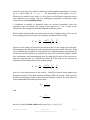
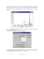
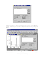
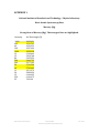
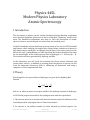
Physics
445L
Modern
Physics
Laboratory
Atomic
Spectroscopy
1
Introduction
The
description
of
atomic
spectra
and
the
Rutherford‐Geiger‐Marsden
experiment
were
the
most
significant
precursors
of
the
so‐called
Bohr
“planetary”
model
of
the
atom.
The
Rutherford
experiment
was
done
in
1909
the
description
of
atomic
spectra,
however,
was
developed
over
more
than
one
hundred
years.
In
1814
Fraunhofer
noticed
dark
lines
in
the
spectrum
of
the
sun.
In
1859
Kirchhoff
and
Bunsen,
while
studying
the
bright
lines
emitted
when
elements
are
heated
to
high
temperatures
noted
that
“an
element
absorbs
lines
in
the
exact
position
as
the
lines
it
can
emit.”
Johann
Balmer,
in
1885
developed
the
formula
that
bears
his
name
for
the
wavelengths
of
the
visible
spectral
lines
of
hydrogen,
λn
=
364.6n2/(n2
‐
4).
This
formula
was
later
generalized
by
Rydberg
and
Ritz.
In
this
laboratory
you
will
study
the
emission
lines
from
various
elements
and
several
other
sources.
In
addition
to
learning
about
the
physics
of
spectra
you
will
learn
the
important
laboratory
skills
of
calibrating
an
instrument
and
using
a
computer
to
collect
experimental
data.
2
Theory
Wavelengths
for
the
spectral
lines
of
hydrogen
are
given
by
the
Rydberg‐Ritz
formula
 1
1
1
= RH  2 − 2  m
λmn
n 
with
n
>
m,
where
m
and
n
are
integers
and
RH
is
the
Rydberg
constant
for
hydrogen.
€
In
1913
Bohr
proposed
a
model
for
the
hydrogen
atom
with
three
postulates.
1.
The
electron
moves
in
a
circular
orbit
about
the
nucleus
under
the
influence
of
the
Coulomb
potential,
obeying
the
laws
of
classical
mechanics
.
2.
In
contrast
to
the
infinite
number
of
orbits
allowed
by
classical
physics,
the
Department
of
Physics
11/24/2009
University
of
Missouri‐Kansas
City
1
of
10
electron
can
occupy
only
orbits
for
which
its
orbital
angular
momentum,
Ln,
is
given
by
Ln
=
nh/2π
where
n
=
1,
2,
3,
...
.
We
frequently
use
the
symbol
 = h /2π .
Electrons
are
stable
in
such
orbits,
i.e.,
they
have
a
well
defined
energy
and
do
not
emit
radiation
even
though
they
are
undergoing
centripetal
acceleration.
Bohr
termed
these
orbits
stationary
states.
€
3.
Radiation
is
emitted
or
absorbed
when
an
electron
transitions
from
one
stationary
state
to
another.
The
energy
of
the
radiation,
E
=
hν,
is
equal
to
the
difference
in
the
energies
of
the
initial
and
final
stationary
states.
Bohr’s
model
predicted
that
a
transition
from
a
state
of
higher
energy
(ni)
to
one
of
lower
energy
(nf)
should
result
in
the
emission
of
radiation
with
energy
hc
mZ 2e 4  1
1
Ei − E f =
=
−


λ (4 πε0 ) 2 2 2  n 2f n i2 
where
Z
is
the
number
of
protons
in
the
nucleus
and
e
is
the
charge
of
the
electron.
Unfortunately,
this
did
not
agree
with
experimental
spectral
results.
Therefore,
Bohr
soon
modified
€
his
postulates
to
require
that
the
combined
angular
momentum
of
the
electron
and
the
nucleus,
be
quantized
in
units
of
h/2π
which
brought
his
model
into
conformance
with
experimental
data.
By
replacing
the
mass
of
the
electron
m,
with
the
reduced
mass
µ =
mM/(M+m)
where
M
is
the
mass
of
the
nucleus,
he
obtained
the
following
result
for
the
emitted
energy:
hc
µX Z 2e 4  1
1
€
Ei − E f =
=
−


λ (4 πε0 ) 2 2 2  n 2f n i2 
here
µX
is
the
reduced
mass
of
the
atom
X.
Using
the
reduced
mass
implies
that
different
isotopes
of
the
same
element
will
have
different
spectra.
Bohr
used
his
€
model
of
the
hydrogen
atom
to
show
that
the
Rydberg
constant,
RH,
was
related
to
other
fundamental
constants
by
the
formula
e2
RH =
8πε0 a0 hc
and
€
e2
h=
8πε0 a0 R H c
Here
a0
is
called
the
Bohr
radius
and
is
given
by
a0 = 4 πε0 2 /me e 2 €
Department
of
Physics
11/24/2009
University
of
Missouri‐Kansas
City
€
2
of
10
3
The
Experiments
3.1
Apparatus
The
apparatus
for
these
experiments
consists
of
several
light
sources,
an
optical
fiber
for
directing
the
light
into
the
spectrometer,
which
consists
of
a
rotatable
grating
and
two
mirrors
for
directing
the
light,
a
solid
state
detector,
and
a
computer
for
recording
the
data.
Here
is
a
picture
of
the
spectrometer
and
the
detector.
Figure
1
Oriel
spectrograph
and
detector
Figure
2
Lamp
3.2
Setup
First,
read
the
Spectra‐Array
software
user
manual
and
MS
125
1/8m
spectrograph
model
77400
documents.
Familiarize
yourself
with
the
instrument
and
the
LineSpec
software.
Second,
it
is
important
that
all
of
the
mechanical
connections
of
the
instrument
be
carefully
and
securely
made
so
that
the
parts
do
not
wobble
out
of
alignment.
If
they
seem
loose,
ask
the
lab
assistant
to
fix
them.
3.3
Calibration
What
is
calibration
and
what
does
it
do?
Department
of
Physics
11/24/2009
University
of
Missouri‐Kansas
City
3
of
10
It
is
not
possible
to
measure
the
wavelength
of
light
directly
so
we
need
to
use
an
indirect
measuring
system.
Indirect
measuring
systems
require
calibration.
Consider
the
gasoline
pump.
In
the
early
days
they
consisted
of
a
glass
cylinder
with
graduations
showing
the
volume
of
gasoline
in
the
cylinder.
The
amount
of
gasoline
purchased
could
be
read
directly
against
these
graduations.
When
pumps
with
rotary
flow
meters
and
mechanical
quantity
displays
came
into
fashion
these
pumps
measured
the
volume
of
gasoline
indirectly
by
counting
the
rotations
and
converting
the
number
of
counts
to
a
volume
that
was
displayed.
These
pumps
required
periodic
calibration
to
ensure
that
the
amount
displayed
was
accurate.
The
spectrograph
used
in
this
experiment
requires
similar
calibration.
(a)
Direct
measure
pump
(b)
Rotary
flow
meter
pump
Figure
3
Although
the
exact
procedure
may
vary
from
instrument
to
instrument,
the
calibration
process
generally
involves
using
the
instrument
to
test
samples
of
one
or
more
known
values
called
calibrants.
The
calibrants
used
in
these
experiments
are
lines
of
very
well
known
wavelengths
from
a
mercury
discharge
tube.
These
lines
fall
onto
pixels
of
the
CCD
detector.
Calibration
is
essentially
the
assignment
of
pixels
to
known
wavelength
values.
Mercury
has
a
distinctive
yellow
doublet
between
approximately
575
and
580
nm
and
a
strong
single
green
line
and
single
violet
line
as
shown
below.
Yellow
doublet
at
578.97
nm
and
576.96
nm
Green
line
546.074
nm
Violet
line
435.833
nm
Department
of
Physics
11/24/2009
University
of
Missouri‐Kansas
City
4
of
10
Figure
4
Location
of
lines
of
mercury
used
for
calibration.
The
first
step
is
to
set
the
grating
of
the
spectrometer
to
546
nm.
When
the
micrometer
is
set
to
4
mm
the
grating
is
approximately
centered
at
400
nm;
5
mm
corresponds
to
500
nm
and
so
forth.
So
5.46
on
the
micrometer
will
move
the
grating
so
that
it
is
approximately
centered
at
546
nm.
To
take
a
sample
spectrum,
select
the
Spectrum
item
from
the
Mode
menu.
Check
the
Sample
box.
Now
select
the
third
button
from
the
left
(Scan
with
Averaging)
near
the
top
of
the
of
the
LineSpec
window.
Enter
100
in
the
number
of
scans
box
and
choose
OK.
The
spectrum
will
appear
in
the
Sample
window
of
the
Dump
window.
You
may
narrow
the
area
around
a
peak
by
using
the
mouse
to
draw
a
selection
box
around
it.
•
To
determine
the
calibration
coefficients
using
a
spectral
calibration
lamp:
Department
of
Physics
11/24/2009
University
of
Missouri‐Kansas
City
5
of
10
1.
Record
the
emission
spectrum
of
a
spectral
calibration
lamp
for
the
appropriate
detector
(Master,
Slave
1,
Slave
2
or
Slave
3.
We
only
have
a
master.).
An
example
of
an
emission
spectrum
corresponding
to
a
spectral
calibration
lamp
is
shown
in
Figure
5.
Figure
5
2.
Select
Wavelength
Calibration
from
the
Setup
pull‐down
menu
to
display
the
Wavelength
calibration
control
window.
Figure
6.
Figure
6
3.
Click
the
Calibrate
using
spectral
lines
button
to
display
the
Find
calibration
for
a
Master
detector
control
window
as
shown
in
Figure
7.
Department
of
Physics
11/24/2009
University
of
Missouri‐Kansas
City
6
of
10
Figure
7
4.
Find
the
position
of
a
known
spectral
line
using
the
mouse
pointer.
Note
the
position
(pixel
units)
of
the
spectral
line
displayed
in
the
status
bar
(see
Figure
8
below):
Figure
8
Department
of
Physics
11/24/2009
University
of
Missouri‐Kansas
City
7
of
10
5.
Click
the
Add
button
in
the
Find
calibration
control
window
to
display
the
following
window:
Figure
9
Enter
the
pixel
position
of
the
spectral
line
and
the
known
position
in
nanometer
units.
6.
Repeat
steps
4
to
5
identifying
at
least
three
spectral
lines
that
span
the
detection
region
of
interest.
It
is
best
to
try
to
use
the
lines
farthest
to
the
left
and
farthest
to
the
right
so
that
your
calibration
equation
is
interpolating
rather
than
extrapolating.
7.
Once
the
features
of
interest
have
been
identified
and
assigned
to
known
spectral
lines,
the
program
automatically
calculates
the
wavelength
calibration
coefficients
as
shown
in
Figure
10:
Department
of
Physics
Figure
10
11/24/2009
University
of
Missouri‐Kansas
City
8
of
10
The
Edit
button
allows
the
user
to
modify
any
reference
points
within
the
table,
while
the
Delete
button
allows
points
to
be
removed.
8.
Click
the
Accept
button
to
automatically
update
the
wavelength
calibration
coefficients
or
Cancel
to
retain
the
original
settings.
3.4
Procedures
Take
several
measurements
of
each
spectrum
and
use
the
mean
as
your
result.
•
Observe
the
spectra
from
the
incandescent
and
the
fluorescent
(overhead)
light
sources
using
the
hand
held
spectroscope.
Describe
these
spectra
qualitatively.
•
Measure
and
record
spectra
from
the
fluorescent
and
incandescent
light
sources
using
the
Oriel
spectrograph.
•
Measure
and
record
lines
from
the
H,
2H
(deuterium),
He,
Ne,
Hg,
and
Xe
lamps.
•
Measure
and
record
lines
from
the
white,
blue
and
red
LEDs.
4
Analysis
When
writing
your
report
include
all
instrument
parameters
such
as
the
grating
constant,
slit
width,
resolution,
focal
lengths,
etc.
Compare
all
of
your
results
to
currently
accepted
standard
values
and
do
error
analyses.
•
Determine
Rydberg’s
constant
for
hydorgen
and
deuterium.
•
Compute
Planck’s
constant.
•
Find
the
ratio
of
the
mass
of
deuterium
to
hydrogen.
•
Determine
the
ground
state
energy
of
hydrogen
by
using
the
Bohr
model
and
the
measured
wavelengths
of
the
lines
in
the
Balmer
series.
Department
of
Physics
11/24/2009
University
of
Missouri‐Kansas
City
9
of
10
APPENDIX
1
National
Institute
of
Standards
and
Technology
­
Physics
Laboratory
Basic
Atomic
Spectroscopy
Data
Mercury
(Hg)
Strong
Lines
of
Mercury
(Hg).
The
strongest
lines
are
highlighted.
Intensity
1000
400
60
100
1000
12
15
80
500
200
50
60
12
20
15
250
25
Air
Wavelength
(Å)
3983.931
4046.563
4339.223
4347.494
4358.328
5128.442
5204.768
5425.253
5460.735
5677.105
5769.598
5790.663
5871.279
5888.939
6146.435
6149.475
7081.90
Department
of
Physics
11/24/2009
University
of
Missouri‐Kansas
City
10
of
10