Download 31295019600575

MODELING HYBRID DOMAINS USING PROCESS
DESCRIPTION LANGUAGE
by
SANDEEP CHINTABATHINA, B.S.
A THESIS
IN
COMPUTER SCIENCE
Submitted to the Graduate Faculty
of Texas Tech University in
Partial Fulfillment of
the Requirements for
the Degree of
MASTER OF SCIENCE
Approved
Chairperson of the Committee
Accepted
Dean of the Graduate School
December, 2004
ACKNOWLEDGEMENTS
I would like to thank my parents and my sister for their support and good
wishes. They have always been my reason to do well. Mother and Father, I would
like to express to \ou my gratitude in your support as I pursue my college education.
And Akka, 1 have learned a lot of things from you over the years. Thank you for
everything.
I would like to thank Dr. Gelfond and Dr. Watson for making this thesis
possible. You guys are good at what you do and also nice to work with. You have
constantly pushed me and got the best out of me. Thank you for your guidance and
support.
Dr. Gelfond working with you is an unforgettable experience. I am amazed by
your ability to concentrate. Your work ethic and moral values will always inspire me.
I have learned so much from you. You always make time for me even when you are so
busy. You worked almost everyday with me to finish this thesis. I really appreciate
it. Thank you for all your suggestions and comments.
Dr. Watson you are a very open-minded and down to earth person. You hired
me as a research assistant at a time when I desperately needed funding. Thank you
for giving me an opportunity. I am glad that I will be one of your first students to
graduate. I am looking forward to working with you in future research projects.
."•Vnd to all my friends at Tcwas Tech University, a big thank you for cheering
me up whene\'er 1 am feeling down.
Ricardo \'()U nvv my hi'sl friend ever.
Whether it is working with you or
playing with you or just hanging out I enjoy every bit of it. Thank you for being
there whenever 1 needed \'ou.
A big thanks to Sunil and all my ex-roommates for bearing with me. Sunil,
we had a great time as roommates, I will never forget that.
1 would like to thank all the KR lab members. Each and everyone has contributed in some wa\' or an other towards this thesis. Its nice to be part of a very
active and smart group of researchers. I enjoy working with you all.
1 would like to thank the faculty and staff of computer science department for
their support and cooperation. Finally, I would Uke to thank NASA Johnson space
center for funding our research projects.
Ill
TABLE OF CONTENTS
ACK.XOWLEDGEMENTS
ABSTRACT
VI
LIST OF FIGURES
vn
1
INTRODUCTION
2
SYNTAX AND SEMANTICS
3
...
2.1
SYNTAX
2.2
SEMANTICS
2.3
S P E C I F Y I N G HISTORY
1
.
...
8
8
.
. .
13
16
TRANSLATION INTO LOGIC PROGRAM .
3.1
DECLARATIONS
3.2
G E N E R A L TRANSLATIONS
3.3
D O M A I N I N D E P E N D E N T AXIOMS
3.4
E X A M P L E TRANSLATIONS
. . . .
. . . .
19
. . . .
19
.
22
. . . .
. .
.
.
.
.
25
28
4
EXAMPLE DOMAIN
5
PLANNING AND DIAGNOSIS
42
5.1
PLANNING
42
5.2
DIAGNOSIS
47
6
.
33
RELATED WORK
6.1
S I T U A T I O N CALCULUS
6.2
L A N G U A G E AVC
60
.
.
.
.
.
60
75
iv
7 CONCLUSIONS AND FUTURE WORK
82
REFERENCES
84
APPENDIX A
. .
86
ABSTRACT
Researchers in the field of knowledge representation and logic programming
are constantly tr>'ing to come up with better ways to rejiresent knowledge. One of the
recent attempts is to model (l\'namic domains. A dynamic domain consists of actions
that are capable of changing the properties of objects in the domain, for example the
blocks world domain. Such domains can be modeled by action theories - collection of
statements in so called action languages specifically designed for this purpose. In this
thesis we extend this work to allow for continuous processes
properties of objects
that change continuously with time. For example the height of a freely falling object.
In order to do this we adopt an action language/logic programming approach.
A new action language called process description language is introduced that
will be useful to model systems that exhibit both continuous and discrete behavior
(also called hybrid systems). An example of a hybrid domain is the domain consisting
of a freely falling object. A freely falling object is in the state of falling,
which is
a discrete property that can be changed only by actions (also called fluent) while its
height is a continuous process.
The syntax, semantics, and translation of the statements of the language into
rules of a logic program will be discussed. Examples of domains that can represented
in this language will be given. In addition, some planning and diagnostic problems
will be discussed. Finally, the language will be compared with other languages used
for similar purposes.
vi
LIST OF FIGURES
1.1
Transitions caused by ./7//'
. .
1.2
Transitions caused l)y drop and cdtch
1.3
Mapping between local and global time
5.1
Architecture of an agent in a hybrid domain
VII
.
.
...
. . .
2
3
5
56
CHAPTER 1
INTRODUCTION
Designing an intelligent agent capable of reasoning, planning and acting in a
changing enxironment is one of the important research ar(>as in the field of AI. Such
an agent should have knowledge about the domain in which it is intended to act
and its capabilities and goals. In this thesis we are interested in agents which view
the world as a dynamical system represented by a transition diagram whose nodes
correspond to possible physical states of the world and whose arcs are labeled by
actions. A hnk, (so,a,Si) of a diagram indicates that action a is executable in SQ
and that after the execution of a in SQ the system may move to state Si. Various
approaches to representation of such diagrams [3; 6; 9] can be classified by languages
used for their description. In this thesis we will adopt the approach in which the
diagrams are represented by action theories
collections of statement in so called
action languages specifically designed for this purpose.
This approach allows for
useful classification of dynamical systems and for the methodology of design and
implementation of deliberative agents based on answer set programming.
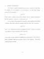
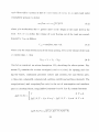
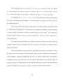
Most of this work, with the notable exception of [4; 14], deals with discrete
dynamical systems. A state of such a system consists of a set of fluents - properties
of the domain whose values can only be changed by actions. An example of a fluent
would be the position of an electrical switch. The position of the switch can be
1
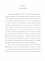
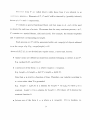
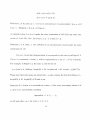
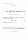
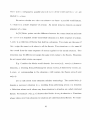
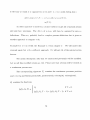
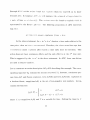
changed onl\' whiMi an external force cau.s(>s it to change. Once changed, it stays
in that position until it is changed yet again. The corresponding transitions in the
diagram are shown in Figure 1.1.
Sl
flrp
on
flip
^
I
-^on
Figure 1.1: Transitions caused by flip
Action languages will describe the diagram in Figure 1.1 by so called dynamic causal
laws of the form:
flip
causes
-^on if
flip
causes
on if
on.
(LI)
^on.
(L2)
(1.1) says that performing the action flip causes the position of the switch to be off
if it was on. (1.2) says that performing the action flip causes the position of the
switch to be on if it was
off.
In this thesis we focus on the design of action languages capable of describing
dynamical systems which allow continuous processes - properties of an object whose
values change continuously with time.
Example of such a process would be the
function, height of a freely falling object.
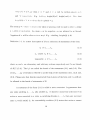
Suppose that a ball, 50 meters above
the ground is dropped. The height of the ball at any time is determined by Newton's
laws of motion. The height varies continuously with time until someone catches the
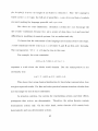
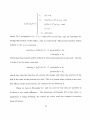
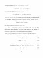
ball before it readies the ground. Suppose that the ball was caught alter 2 seccnuls.
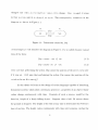
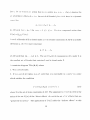
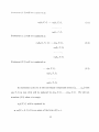
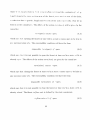
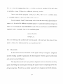
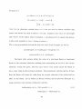
Assume that there is onl\' one arm that drops and catches the ball. Tlie corresponding
transition diagram will contain transitions of the form:
>'0
,S2
Sl
lioldiug
^
drop
I^nght = fo(50,T)
V
[0,0]
y
-'holding
\
catch
height =
f,(50,T)
[0,2]
J
holding
\
height = /o(30.T)
\
[0,5]
where /o and /i are defined as:
fo{Y,T) = Y
f,(Y,T)
=
Y-\gT\
Figure 1.2: Transitions caused by drop and catch
Notice that states of this diagram are represented by mapping of values to the symbols
holding and height over corresponding intervals of time. For example in state S\,
holding is mapped to false and height is defined by the function /i(50,T) where T
ranges over the interval [0,2].
Intuitively, the time interval of a state s denotes the time lapse between occurrences of actions. The lower bound of the interval denotes start time of s which
is the time at which an action initiates s. The upper bound denotes the end time
of s which is the time at which an action teminates s. We assume that actions are
instantaneous that is the actual duration is negligible with respect to the duration of
the units of time in our domain. For computability reasons, we assign local time to
states. Therefore, the start time of every state s is 0 and the end time of s is the time
since the start of .s tih the occurrence of an action terminating s. For example, in
Figure 1.2 the action drop occurs after a time lapse of 0 units since the start of state
So- Therefore, the end time of 5o is 0. The action catch occurs after a time lapse of
2 units since the start of state s^. Therefore the end time of 5i is 2.
The state so in Figure 1.2 has the interval [0,5] associated with it. This interval
was chosen randomly from an arbitrary collection of intervals of the form [0,n] where
n > 0. Therefore, any of the intervals [0,0] or [0,1] or [0, 2] and so on could have been
associated with .so. In other words, performing catch leads to an infinite collection of
states which differ from each other in their durations. The common feature among
all these states is that height is defined by / o ( 3 0 , r ) and holding is true. We do not
allow the interval [0, oo] for any state. We assume that every state is associated with
two symbols
0 and end. The constant 0 denotes the start time of the state and the
symbol end denotes the end time of the state. We will give an accurate definition of
end when we discuss the syntax of the language.
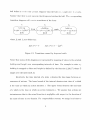
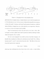
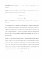
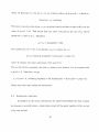
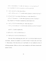
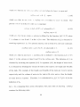
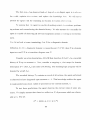
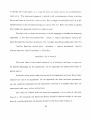
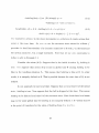
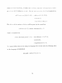
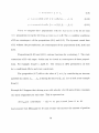
We assume that there is a global clock which is a function that maps every
local time point into global time. Figure 1.3 shows this mapping. Notice that this
mapping allows one to compute the height of the ball at any global time, t G [0, 7].
This is not necessarily true for the value of holding. According to our mapping global
time 0 corresponds to two local times: 0 in state SQ and 0 in state Si. Since the values
of holding in SQ and Si are true and false respectively, the global value of holding at
So
Sl
holding
N
/^
height = fo(50,T)]-^l^hrujhl
S2
-^holding ^
/^
= f,(50,T)\-^^^±^hcigld
Jwldmg~~ .
= ./o(30,T)l
Global
time
(sees)
Figure 1.3: Mapping between local and global time
global time 0 is not uniquely defined. Similar behavior can be observed at global time
2. The phenomena is caused by the presence of (physically impossible) instantaneous
actions in the model. It indicates that 0 and 2 are the points of transition at which the
value of holding is changed from true to false and false to true respectively. Therefore,
it is false at 1 and true during the interval [3,7].
Since the instantaneous actions drop and catch do not have a direct effect
on height, its value at global time 0 and 2 is preserved, thereby resulting in unique
values for height for every t 6 [0, 7].
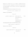
Our new action language H, also called as process description language, will
describe these transitions by defining the continuous process height, fluent holding,
functions fo(Y,T),
fi(Y,T),
and actions drop and catch.
The effects of the action
drop will be given by the causal law:
drop causes
-^holding.
(L3)
which says that performing the action drop at time end in a state, s, causes holding
to be false in the successor stale of .s. This explains the change in the value of holding
from .So to .S]. The executal)ill\' conditions will have the form:
iiiijHi.ssible droj) if
-^holding.
(L4)
which says that the ball cannot be dropped at time end in a state, s, if holding the
ball is false. Therefore, the action drop cannot be performed in the state Si.
impossible
drop if
height(end)
=
0.
(1.5)
sa>'s that the ball cannot be dropped at time end in a state, s, if it is on the ground at
end. height(end)
is a special fluent corresponding to the continuous process height
that denotes the height at the end of a state. The effects of the action catch are given
by the causal law:
catch causes
holding.
(1.6)
(1.6) explains why there is a change in the value of holding from Si to S2- The
executablity conditions will have the form:
impossible
catch if
holding.
(1.7)
(1.7) explains why the action catch cannot be performed in the states SQ and S2.
height is defined by the following statements:
height = fo(Y,T)
if height(0) = Y,
holding.
(1.8)
From Figure 1.3 it is obvious that the value of liciglil is determined depending on
whether holding is true or not. Statement (1.8) re(|uires that in any state in which
holding is true, height does not change with time
h('ight(0) is a special fluent
corresponding to continuous jirocess Iwighl that denotes the lic/ghl at time 0 of a
state. If holding is false then licight is defined as follows:
height = fi(Y,T)
if height(0) = Y,
(1.9)
-'holding.
Statement (1.9) requires that in any state in which holding is false, height is defined
b\' Newtonian equations.
In the next chapter we will discuss the syntax and semantics of the language
and see some more examples.
CHAPTER 2
SYNTAX AND SEMANTICS
2.1
S^•NTAX
To define our language we first need to fix a collection A of time points.
Normally A will be equal to the set, /?+, of non-negative real numbers, but we can as
well use integers, rational numbers, etc. We will use the variable T for the elements
of A. \\"e will also need a collection, Q, of functions defined on A, which we will use
to define continuous processes. Elements of Q will be denoted by lower case greek
letters a, p, etc.
A process description language, i / ( E , ^ , A ) , will be parameterized by A, Q
and a typed signature S. Whenever possible the parameters S, Q, A will be omitted.
We assume that E contains regular mathematical symbols including 0,1, + - , < , < , >
, ^ , *. etc. In addition, it contains two special classes, A and P = J^U C oi symbols
called actions and processes.
Elements of A are elementary actions. A set { a i , . . . , a„} of elementary actions
performed simultaneously is called a compound action. By actions we mean both
elementary and compound actions. Actions wiU be denoted by a's. Two types of
actions
agent and exogenous are allowed, agent actions are performed by an agent
and exogenous actions performed by nature.
Proc(>sses irom J^ are called fluents while those from C are referred to as
coiitiiiMvi.s processes. Elements of V, T and C wiU be denoted by (possibly indexed)
letters p"s, /.-'s and r's respectively.
T contains a special functional fluent end that maps to A. end will be used
to denote the end time of a state. We assume that for every continous process, c € C,
T contains two special fluents, c(0) and c(end). For example, the fluents height(0)
and hcight(end)
corresponding to height.
Each process p e V will be associated with a set range(p) of objects referred
to as the range of p. E.g. range(height)
= i?+
Atoms of 77(S. Q, A) are divided into regular atoms, c-atoms and
f-atoms.
• regular atoms are defined as usual from symbols belonging to neither A nor V.
E.g. mother(X,Y), sqrt(X)=Y.
• c-atoms are of the form c = a where range(c) =
E.g. height — 0, height = fo(Y,T),
range(a).
height = /o(50,T).
Note that a is strictly a function of time. Therefore, any variable occurring in
a c-atom other than T is grounded.
E.g.
height = fo(Y,T)
is a schema for height = XT.fo(y,T)
where y is a
constant, height = 0 is a schema for height = XT.O where AT.O denotes the
constant function 0.
• f-atoms
axe of the form k = y where y G range(k).
If k is boolean, i.e.
rangc(k)
= { T , l } then k = T and k = ± wiU be written siiiii)iy as A-
and ^A' ri\sp(H'ti\-(4y. E.g. holding, height(0)=Y, height(end)=(). N(jte that
luujht{0)
= V is a .schema for hcight{0) = y.
The atom p = v where c (leiR)tes the value of process p wiU be u.sed to refer to either
a c-atom or an f-atom.
An atom (/ or its negation -^u are referred to as literals.
Negation of = will be often written as 7^. E.g. -^holding, height(0) / 20.
Definition 2.1 An action description of / / is a collection of statements of the form:
/o if lu-..,ln-
(2.1)
Ce causes IQ if li,...,ln-
(2.2)
impossible a if / i , . . . , / „ .
(2.3)
where Qg and a are elementary and arbitrary actions respectively and Vs are literals
of H(T..Q,A).
The /Q'S are called the heads of the statements (2.1) and (2.2). The
set {/i,..., /„} of hterals is referred to as the body of the statements (2.1), (2.2) and,
(2.3). Please note that literals constructed from f-atoms of the form end = y will not
be allowed in the heads of statements of H.
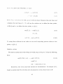
A statement of the form (2.1) is called a state constraint. It guarantees that
any state satifying / i , . . . , /„ also satisfies IQ. A dynamic causal law (2.2) says if an
action a were executed in a state SQ satisfying literals / i , . . . ,/„ then any successor
state Sl would satisfy IQ- An executability condition (2.3) states that action a cannot
10
be executed in a state satisfying / j , . . . , /„. If n = 0 then /,/ is dropped from (2.1),
(2.2), (2.3).
Example 2.1 Let us now construct an action description ADQ describing the transition
diagram from Figure 1.2. Let Go contain functions
foiY,T) = Y.
f,(Y^T)
where Y G range(height),
=
Y-\gT\
g is acceleration due to gravity, and T is a variable for
time points.
The description is given in language H whose signature EQ contains actions drop and
catch, a continuous process height, and fluents holding, height(0) and
holding is a boolean fluent; range(height)
height(end).
is the set of non-negative real numbers. It
is easy to see that statements (1.3) and (1.6) are dynamic causal laws while statements
(1.4), (1.5) and (1.7) are executabihty conditions and statements (1.8) and (1.9) are
state constraints.
Example 2.2 This example is simplied version of the example used by Reiter in [14].
Consider an elastic ball moving with uniform velocity on a frictionless floor between
two walls, Wi and W2. Assume that the floor is the X-axis and the walls are parallel
to the Y-axis. We expect the ball to bounce indefinitely between the two walls. The
bouncing causes velocity of the ball to change discontinuously. And as long as the
velocity is not zero, position changes continuously with time.
11
Let us now construct an action description AD^ of / / ( S i , ^ i , A ) that will
enable us to define the rclociig and position, of the ball. Signature Ei contains the
action bounce(\V)
process position,
which denotes the baU bouncing against wall 11'', a continuous
and fluents velocity, posttion(0)
and
position{end).
Since velocity is uniform and is a changed only by bounce we treat it as a
fluent. The range (velocity) is the set of real numbers and the range(position)
is the
set of non-negative real numbers. Let Qi contain the function
/2(Vo, r , T ) =
^0
if T = 0.
f,(Yo,V,T-l)
where VQ G range(position)
+V
and V G range(velocity).
if T > 0 .
On hitting a wall, the bah
changes direction. This is defined by the causal law:
bounce(\V)
causes
velocity = —V if velocity = V.
(2.4)
Statement (2.4) says that if the ball moving with velocity V bounces against the wall
\V at time end in a state, s, then its new velocity is —1/ in any successor state of s.
position will be defined by the state constraint.
position = f2iYo, V, T) if position(0)
= IQ,
(2.5)
velocity = V.
Statement (2.5) says that position is defined by Newtonian equations in any state.
The occurrence times of the bounce action is determined by Newtonian equations.
One way to represent such an action is to write statements called action triggers that
12
include these Newtonian equations. In general, action triggers describe the effects of
processes or actions on other actions. We will not address the issue of how to write
triggers in this thesis because it is not the purpose of this thesis. Our future work
may involve extending language H to include triggers.
2.2
SEMANTICS
The semantics of process description language, H, is similar to the semantics
of action language B given by McCain and Turner [10; 11]. An action description AD
of H, describes a transition diagram, TD(AD), whose nodes represent possible states
of the world and whose arcs are labeled by actions. Whenever possible the parameter
AD will be omitted.
Definition 2.2 An interpretation, I, of 7/ is a mapping that assigns (properly typed)
values to the processes of H such that for every continuous process, c, I(c(end))
I(c)(I(end))
=
and /(c(0)) = /(c)(0).
A mapping IQ below is an example of an interpretation of action language of Example 2.1.
lo(end) = 0,
lo(holding) = T,
Io(height(0))
13
= 50,
lQ(h<ight(cnd)) = 50,
/n(//cay/,/) = /o(.50,T).
Definition 2.3 An atom p = r is true in interpretation I (symbolically / |= p = t-) if
l{p) = V. Similarly, 1 ^ p ^ v \[ I(p) ^ v.
Aw interpretation / is closed under the state constraints of AD if for any state constraint (2.1) of AD, / 1= /, for every \,l<i<n
then / [= IQ.
Definition 2.4 A state, s, of a TD(AD) is an interpretation closed under the state
constraints of AD.
It is eas>' to see that interpretation IQ corresponds to the state SQ in Figure 1.2.
Wheiic\'er convenient, a state, s, wifl be represented by a set {/ : s |= /} of literals.
For example, in Figure 1.2, the state SQ will be the set
So = {end = 0, holding, height(0) = 50, height(end) = 50, height = /o(50,T)}
Please note that only atoms are shown here. So also contains the literals holding 7^ L,
height(0) / 10, height(0) 7^ 20 and so on.
Definition 2.5 Action a is executable in a state, s, if for every non-empty subset a' of
a, there is no executability condition
impossible a' if / i , . . . , /„.
of AD such that s |= /, for every i, 1 < i <n.
14
Let (/, be an elementar\' action that is executable in a st;ite .s. Es(a,.) denotes the
.set of all direct effects of a,., i.e. the set of all literals IQ for whi( h there is a dynamic
causal law
Oe causes
IQ if
li,.
. . ,l„
in AD such that .s- |= /, for e\'ery ?, 1 < i < n . If a is a compound action then
E4a) = Ua,eaEs{ae).
A set L of literals of H is closed under a set Z of state constraints of AD if L includes
the head, IQ, of every state constraint
IQ if Ix,...
,ln
of AD such that {/i, . . . , / „ } C L. The set Cnz{L)
of consequences of L under Z is
the smallest set of literals that contains L and is closed under Z.
A transition diagram T D = ( $ , ^ ) where
1. $ is a set of states.
2. ^ is a set of all triples (s, a, s') such that a is executable in s and s' is a state
which satisfies the condition
s' = Cnz(E,(a)
U (s n s' ) )
(2.6)
where Z is the set of state constraints of AD. The argument to Cn(Z) in (2.6) is the
union of the set Es(a) of the "direct effects" of a with the set s n s' of facts that are
"preserved by inertia"
The apphcation of Cn{Z) adds the "indirect effects" to this
15
union. In Example 2.1, the set E.Jdrop)
of direct effects of drop will he defined as
Esg(drop) =
{-'holding).
The instantaneous action drop occurs at global time 0 and has no direct effect on the
value of height at 0. This means that the value of height at the end of SQ will be
preserved at time 0 of Si. Therefore,
SoOsj = {height(0) = 50}.
The apphcation of CniZ)
to Eso(drop) U (SQ fl Si) gives the set
Q = {^holding, height(0) = 50, height = /i(50,T)}
where Z contains the state constraints (1.8) and (1.9).
The set Q will not represent the state Si unless end is defined. Let us suppose that
Si(end) = 2. Therefore, we get
Sl = {end = 2, -'holding, height(0) = 50, height(end)
= 30, height = /i(50, T)}.
Please note that only atoms are shown here.
2.3
S P E C I F Y I N G HISTORY
In addition to the action description, the agent's knowledge base may contain
the domain's recorded history - observations made by the agent together with a record
of its own actions.
16
The recorded history defines a collection of patlis in the diagram which, from
the standpoint of the agent, can be interpreted as the .system's possible pasts. If
the agent's knowledge is complete (e.g., it has complete informati(jn about the initial
state and the occurrence's of actions, and the system's actions are determinist ic) then
there is only one such path.
The Recorded history, r „ , of a system up to a current moment n is a collection
of observations, that is statements of the form:
obs(v,p,
t,i).
hpd(a, t,i).
where / is an integer from the interval [0,n) and time point, ^ G A. i is an index of
the trajectory. For example, i = 5 denotes the step 5 of the trajectory reached after
performing a sequence of 5 actions.
obs(v,p,t,i)
means that process p was observed to have value v at time t of
step i. hpd(a,t,i)
means that action a was observed to have happened at time t of
step i. Observations of the form obs(y,p, 0,0) will refer to the initial state of the
system.
Definition 2.6 A pair {AD, F) where AD is an action decription of H and F is a set
of observations, is called a domain
description.
17
Definition 2.7 (iiven an action decription AD of II that describes a transition diagram
TD(AD), and recorded history. F,,, upto moment n. a ])a,th
(.s'o,ao,Si,.. . ,r;„_i,s.„)
in the TD(AD) is a model of P,, with respect to the domain description, (/lL',r„), if
for every /, 0 < / < n and / G A
1. a, = {a : hpd(a, 1.1) G r „ } :
2. if obs(v.p, t. i) G r „ then p = v E s,.
18
CHAPTER 3
TR.ANSL.VTION INTO LOGIC PROGRAM
In this chapter we will discuss the translation of a domain description written
in language H into rules of an A-Prolog program. A-Prolog is a language of logic
programs under the answer set semantics [5] for representing agent's knowledge about
the domain and formulating the agent's reasoning tasks. Since we use SMODELS [12]
to compute answer sets of the resulting A-Prolog program, the translation will comply
with the syntax of the SMODELS inference engine.
Gi\en a domain description, V = {AD, F) where AD is an action description
of H and F is a set of observations, we will construct the logic program, aQ(T>) by
mapping statements of T> into rules of A-Prolog.
aQ(T>) contains two parts. The first part contains declarations for actions and
processes and the second part contains translations for the statements of H and the
observations in P.
3.1
DECLARATIONS
Let us look at a general way of declaring actions and processes:
action(action-name,
process(procesS-name,
19
action-type).
process-type).
acturn-iiame and actionJype
are non-numeric constants denoting the name of an
action and its type respectively. Similarly, proccss-namc and processJype are nonnumeric ci)iistaiits denoting the name of a i)rocess and its type respectively.
For
instance in Example 2.1 the actions and processes are declared as follows:
action(drop, ag( nt).
action(catch,
agent).
process (height,
continuous).
process(holding,
fluent).
Now let us see how the range of a process is declared. There are a couple
of wa\s of doing this. The range of height from Example 2.1 is the set of nonnegative real numbers. In terms of logic programming this means infinite groundings.
Therefore, we made a compromise and chose integers ranging from 0 to 50.
values(0..50).
range(height,Y)
: — values(Y).
holding is a boolean fluent. Therefore, we write
range(holding,
true).
range(holding,
false).
Suppose we have a switch that can be set in three different positions, the range of
20
the process swilcti-position is declared as:
rangi (suritchjposition,
low).
rangc(swi.tch-p(>sition,
medium).
ran ge(swi I eh ^position, high).
In order to talk about the \'alues of processes and occurrences of actions we
have to consider the time and step parameters.
Integers from some interval [0, n] will be used to denote the step of a trajectory.
Ls will be used as \-ariables for step. Now every step has a duration associated with
it. Therefore, integers from some interval [0, m] will be used to denote the time points
of ever>' step. In this case, m will be the maximum allowed duration for any step.
T"s will be used as variables for time. Therefore, we write
step{0..n).
time(0..m).
Assume that n and m are sufficiently large for our applications. Then we add the
rules
H^domain step(I;
^domain
II).
time(T; Tl; T2).
for declaring the variables / , 71, T, Tl and, T2 in the language of SMODELS. The
first domain declaration asserts that the variables / and 71 should get their domain
from the literal
step(I).
21
:^2
G E N E R A L TRANSLATIONS
Let us look at a general translation of an action description of H into rules
of A-prolog.
If a is an elementary action occurring in a statement that is being
translated, it is translated as
o(a,T,I)
which is read as "action a occurs at time T of step /." If a is a compound action then
for each elementary action Og G a, we write
o(ae,T,I).
If / is a literal of H occurring in the any part of the statement that is being
translated, other than the head of a dynamic causal law then it will be written as
cyo{l,T,l).
ao(l, T. I) is a function that denotes a translation of hteral /. A hteral, /, occurring
in the head of a dynamic causal law will be written as
ao(/, 0,7 + 1).
In this thesis we limit ourselves to translating action descriptions of H in which the
heads of dynamic causal laws are either f-atoms
translations look as follows:
•79
or their negations.
The general
StattMiient (2.1) will be translattnl as
aQ(k,T,I):-
ao(h,T,I),
(3.1)
ao{l„.TJ).
Statement (2.2) wiU be translated as
aQ(lQ,0,I + l):-
o(ae,T,I),
(3.2)
ao(^i,7',/).
O!0(ln,T,I).
Statement (2.3) will be translated as
•.-o(a,T,I),
(3.3)
0!o{luT,I),
ao(ln,T,I).
In statement (2.3) if a is the non-empty compound action { a i , . . . , 0 ^ } then
o(a,T,I)
in rule (3.3) wiU be replaced by o(ai,T,I),...
translate (2.3) when a is empty.
ao(l,T,I)
wiU be replaced by
• val(V, c, 0, / ) if / is an atom of the form c(0) = v.
23
,o(am,T,I).
We wifl not
val(\'.c.{).l)
is read as " \ ' /.s the value of process c at tviiie 0 of step /."
E.g. height{0) = Y will hv tran.slated as val{\
• - r a / ( r . c , 0 , 7) ff / is of the form c(0)
-val{\ .c,0,I)
,h.eig}it,0,1).
^v.
is read as "U /,s not the value of process c at time 0 of step /."
• ('a/(\ > , T, / ) if / is an atom of the form p = v other than c(0) = v.
val{\',p. T. I) is read as " U is the value of process p at time T of step 7."
E.g. height(cnd)
= 0 wiU be translated as val(0, height,
T,S).
• -val{\', p. T. I) if / is of the form p j^ v other than c(0) ^ v.
-valiWp.
T. I) is read as " V is not the value of process p at time T of step I."
ao(l, 0, 7 + 1) will be replaced by
• val(V.p, 0, 7 -I- 1) if / is of the form p = v.
• —val(V, p, 0,7 + 1) if / is of the form p ^ v.
Note that when translating the f-atom,
end = y we will not follow the above
conventions. Instead we translate it as end(T, I) where T denotes the end of step
/ . Observations of the form obs(v,p,t,i)
and hpd(a,t,i)
are translated as facts of
A-Prolog programs. Before we look at some examples we will discuss domain independent axioms.
24
3.3
DOKL-XIN I N D E P E N D E N T A X K ) M S
Domain independent axioms define properties that are common to every domain. Wi> will denote such a colli>ction of axioms by H. Given a domain description
V. and nii(P) that maps V into rules of .A-prolog, we wiU ccjiistruct a(V) that adds
n to ao(P). Therefore,
o(P) = n U a o ( P ) .
Let us look at the axioms constituting H.
E N D O F STATE AXIOMS
These axioms will define the end of every state s. The end of a state is the local
time at which an action terminates s. When it comes to implementation we talk
about the end of a step instead of state. Therefore, we write
end(T,I):-o{A,T,I).
(3.4)
If no action occurs during a step then end will be the maximum time point allowed
for that step. This is accomplished by using the choice rule
{end(m,I)}l.
(3.5)
The consequence of the rule (3.5) is that the number of end(m,I) that will be true is
either 0 or 1. A .step cannot have more than one end. This is expressed by (3.6).
: - end(T\,I),
end(T2,I),
neq(Tl,T2).
25
(3.6)
Every sUp must end. Therefore, we write
ends(l)
: - cn,l(T,l).
(3.7)
: - not cnils(l).
(3.8)
Ever>- step. i. is associatetl with an interval [0,e] where 0 denotes the start time and
e denotes the end time of i. We will use the relation out to define the time points,
t ^ [0, e] and in to define the time points, t G [0, e].
out(T,I)
: - end(Tl,I),
(3.9)
T>Tl.
in(T.I):
-not outiT,I).
(3.10)
By using these relations in our rules we can avoid computing process values at time
points, / ^ [0,e].
INERTIA AXIOM
The inertia axiom states that things normally stay as they are. It has the following
form:
val(Y,P,0,I-\-l)
:-
val(Y.P,T,I),
(3.11)
end(T, I),
not -val(Y,P,0,I
+ 1).
Intuitively, rule (3.11) says that actions are instantaneous. In example (2.1),
height at global time 0 is 50 when the instantaneous action drop occurs at 0.
26
RKALITY CHECK AXIOM
This axiom guarante(\s that the agent's predictions match with his observations.
:-
ob.s{},P,T,I),
(3.12)
'^val{},P,T,I).
O T H E R AXIOMS
The axiom
o(A,T,I):-hpd{A.T,I).
(3.13)
sa>-s that if action A was observed to have happened at time T of step I then it must
ha\'e occurred at time T of step I. And we have
val{Y, P, 0,0) : - obs(Y. P, 0.0).
(3.14)
for defining the initial values of processes. A fluent remains constant throughout the
duration of a step. This is expressed by the axiom (3.15).
val(Y, P, T,I):-
val(Y, P, 0,1),
process(P,
(3.15)
fluent),
in(T,I).
Axiom (3.16) says that no process can have more than one value at the same time.
-val(Yl,P,T,I)
:-
val(Y2,P,T,I),
neq(Yl,Y2}.
27
(3.16)
3.4
E X A M P L E TRANSL.ATIONS
Now let us refer back to Examples 2.1 and 2.2 and see how the corresponding causal
laws will be translated. In Example 2.1 tlu' dynamic causal law
drop caus(s
-'holding.
is translated as
val(false,
holding, 0, 7 -I- 1) : -o(drop, T, I).
catch causes
holding.
is translated as
val{true, holding, 0,7 + 1) : —o(catch, T, I).
Next we look at the executability conditions.
impossible
drop if
^holding.
is translated as
:-
o(drop,T,I),
val(false,
impossible
holding, T, I).
drop if
height(end)
is translated as
28
=0
:-
o(drop,T,I),
val(0,li.eight,T,I).
impossible
catch if
holding
is translated as
: — o{catch,T,
I),
val(true, holding, T, I).
Next we look at state constraints.
height = /o(>',r) if height(0) = Y,
holding.
is translated as
function
val(fO(Y,T),height,T,I)
fO.
: - val(Y, height, 0,1),
val(true, holding, T, I),
in(T,I),
range(height,
Y).
The function /O is a user defined function that is linked to Iparse. Such functions
29
are meant to be called directly from logic programs. Not(> that the function has to
be declared before it appears in aii.\' rule. For more information on how to use them
refer to the Iparse user manual.
height = fiiY.T)
if hcujht(0) = Y.
^holding.
is translated as
function
val(fl(Y.T),
fl.
height, T, I) : - val{Y, height,
0,1),
val{false, holding, T, I),
in(T,I),
range(height,
i').
where / I is also a user defined function that is linked to Iparse. The value returned
by the function fl given Y and T, will determine the value of height at T.
Now let us look at the translations for the causal laws in Example 2.2. The
dynamic causal law
bounce(\V)
causes
velocity = V if
is translated as
30
velocity = —V.
ra/(n,('c/o('/7//, 0,7 + 1) : - o{hounce{W),T,
I),
val(V,velocily,T,I),
VI = - 1 * 1 / ,
(/'a//(ir),
range(velocity,
V),
range(velocity,
VI).
And the state constraint
position = /2(Vo, \', T) if position(0)
= YQ,
velocity = V.
is translated as
val(f2(Y0,
V,T),position,T,
I) : — val{YO,position,
0,1),
val(V, velocity, T, I),
in(T,I),
range(position,
YO),
range(velocity,
V).
where / 2 is a user defined function. The following hypothesis establishes the relationship between the theory of actions in H and logic programming.
31
HYPOTHESIS
Given a domain description V — {AD,T„)
wliere AD is an action descri])tion of
7 / ( E , ^ , A) and r „ is the recorded history upto moment n; if the initial situation of
r „ is complete,
i.e. for any process /) of E. r „ contains o6s(e,p, 0,0) then M is a
model of r „ iff M is defined by some answer set of a ( P ) .
A proof of the above hypothesis will not be presented in this thesis. If proven it
means that our translations are indeed correct. In the next chapter we will look at a
complex example and some experimental results.
32
CHAPTER 4
LNAMPLE DOMAIN
In this chapter we will look at an example domain and show how our language
can be used to model it. First we will understand the physics of the system and then
construct an action description describing the system. Later we wifl translate the
statements of the action description into rules of A-prolog. Finally, we will look at
some sample scenarios and experimental results.
Example 4.1 Consider a rectangular water tank with a faucet on the top and a drain
at the bottom. The faucet is the source of water to the tank and the drain is an
outlet. The faucet can be opened and closed. We are interested in predicting the
volume of water in the tank. Let us first understand the physics of the system.
Assume that the velocity at which the water flows out of the faucet into the tank
(called inflow rate) is approximately 3 m/sec when the faucet is open and 0 when it
is closed. The volume of water flowing into the tank per second, denoted by Vin, is
determined by the following equation:
Vin = in flow-rate
* cf.
(4.1)
where cf is the cross section area of the faucet opening. Now we will define the
outflow rate which is the velocity at which the water flows out of the drain. We
33
api4\- BernouUi's eciuation of law of const-rvation of energy to an open tank under
atmospheric pressure^ to derive
out flow jiiU = J2 * g * h.
(4.2)
where g is acceleration due tt) gravity and /; is the height of the water level in the
tank. Now we can define the volume of water flowing out of the tank per second,
denoted In' Vout, as follows
\'uut = outflow-rate
* cd.
(4.3)
where cd is the cross section area of the drain opening. If Vf is the volume of the tank
at current time, t, then
Vt+l = Vt + Yn - Vout-
(4.4)
Now let us construct an action description AD2 describing the above system. Signature E2 contains the actions turn(open)
and turn{close)
for opening and clos-
ing the faucet, continuous processes volume and outflow-rate
inflowjrate,
range(volume)
volume(0),
volume(end),
outflow-rate{0)
and fluents open,
and outflow-rate(end).
The
and range(out flow -rate) is the set of non-negative real numbers;
open is a boolean fluent; range(inflow) contains 0 and 3. Let Q2 contain functions
Y
fs(Y,N,T)
ff
T = 0.
=
' fs(Y,N,T-l)-\-N*cf-f,(Y,N,T-l)*cd
f,(Y,N,T)
=
p*g*f,(Y.N,T)/(Ub).
34
ii T > 0.
where Y G range{volu.mc),
N G riingc{inflow-rale)
and the constants cf, cd. g,
I and b denote the cross .section area of the faucet, cross section area of the drain,
acceleration due io gravit>', length and l)readth of the tank respectively. Now let us
look us at the causal laws. The effects of the action tu.rn(opcn) will be given by the
causal law
turn(open)
causes
open.
(4-5)
which sa>'s t hat opening the faucet at time end in a state s causes open to be true in
any successor state of s. The executability condition will have the form
impossible
turn(open)
if
open.
(4-6)
which says that it is not possible to open the faucet at time end in a state s if it is
already open. The effects of the action turn(close)
turn(close)
causes
are given by the causal law
-'open.
(4-7)
which says that closing the faucet at time end in a state s causes open to be false in
any successor state of s. The executability condition will have the form
impossible
turn(close)
if
-'open.
(4.8)
which says that it is not possible to close the faucet at time end in a state s if it is
already closed. The fluent inflow-rate
inflow-rate
is defined by the state constraints
= 3 if
35
open.
(4.9)
which savs that in any state, s, infloiv-valc
infloivj-al(
is 3 when the faucet, is open and
= 0 / / -'Open.
which says that in any state, .s, inflowj-alc
(4.10)
is 0 when the faucet is closed. The
process volume is defined by the state constraint
volume = fs{],N,T)
if volume(0) = V.
inflow-rate
(4.11)
= N.
which says that in aii\' state, s, volume is defined by the function f3(Y,N,T)
V is volume at time 0 and A' is the inflow-rate.
rewriting equation (4.4). The process outflow.rate
out flow-rate
= f4i\',N,T)
The definition of /a is obtained by
is defined by the state constraint
if volume(0) = Y.
inflow-rate
which says that in any state, s. out flowjrate
where
(4.12)
= N.
is defined by the function
where Y is the volume at time 0 and N is the inflowjrate.
fA(Y,N.T)
The definition of f^ is
obtained by rewriting the equation (4.2). In equation (4.2), the height of water level,
h, is obtained by dividing the volume of water in the tank by the length and breadth
of the tank. For example, if the length and breadth of the tank are 3 and 4 meters
respectively and the volume of water in the tank is 36 cubic meters, then the height
of water level is 3 meters. Therefore, h is substituted by f3,(Y,N,T)/(l
* b) in the
definition of f^.
Let a be a mapping from action description AD2 into rules of A-prolog.
contains the following rules:
36
a(AD2)
Statement (4.5) is translated as
;•(//(/;•;/('. o/)c/;, 0,7 + 1) : - o{turn{opeii),T,
I).
(4.13)
Statement (4.6) is translated as
: - o(turn(open),T,I),
(4.14)
val[tru.e,open,T,I).
Statement (4.7) is translated as
val(false,
open, 0,7 + 1) : -o(turn(close),T,
I).
(4.15)
And (4.8) is translated as
: - o(turn(close),T,I),
val(false,
(4.16)
open, T, I).
Statement (4.9) is translated as
val(3,inflow-rate,T,I)
: -val(true,open,T,I).
(4.17)
And (4.10) is translated as
val(0,inflow-rate,T,
I) : —val(false,open,T,I).
(4.18)
Statement (4.11) contains a complex recursive function f^ which in turn calls
the function f^. One way of implementing such functions is to link them to Iparse.
Lparse uses pointer arithmetic to deal with the arguments of the user defined functions. It is capable of handling simple recursion but fails to give expected results when
37
functions interact recursively with each otlier. Therefore, we simplify these functions
consideraiily. so that Iparse lan handle them. Therefore the traiislati(jns of (4.11) and
(4.12) contain modified versions of fi and /4. W'c wiU call these modified versions as
/a and f[ respecti\'ely.
The following equation defines the relationship l^etween fs and f^.
f',iYN,T)
= f,{),N,l)
If
f,(YQ,N,T-l)
= Y
Therefore, (4.11) is translated as
function
val{f3'('t'0.A).volume,T-\rl,I)
/3'
: - val(Y0, volume,T, I),
val(N, inflow-rate,
(4.19)
T, I),
in(T+l,I),
range(in flow-rate,
range(volume,
N),
YO).
The following equation defines the relationship between f^ and f'^.
f',(Y,T)
= f,(Y,N,0)
if
fs(YQ,N,T)=Y
Therefore, (4.12) is translated as
function
val(fA'(Y),outflow.rate,T,I)
/4'.
: - val(\ , volume, T, I),
range(volume,
38
V).
(4.20)
For a comiilete listing of the translations along with declarations and domain independent axioms please refer to Appendix A.
S A M P L E SCENARIO AND RESULTS
Let r be the collection of observations:
obs(25, volume, 0, 0).
obs(false, open, 0, 0).
hpd(turn(open),
0,0).
hpd(turn(close),3.1).
The program a(AD2.r)
is obtained by adding F to Q ' ( ^ D 2 ) - In order to run this
program the variables and processes are declared as usual. For instance. I and T take
integer values from the intervals [0,2] and [0,6] respectively, range (volume) is the set
of integers from the interval [0,60].
The program was run on Sparc Ultra 10 running Solaris 8 using the 1.0.9 version of Iparse and 2.26 version of SMODELS. The corresponding answer set returned
from the program was as expected. The average run time was 7.2 seconds of which
SMODELS took 3.3 seconds and Iparse and SMODELS together took 7 seconds.
SMODELS directives are used to get a better looking output. The resulting answer
set is:
39
% proccs.s-nainc{\'alue.
Local-tiiiie.
Sici)).
oulflou<-rale(6, 0, 0).
eo/(/7?U'(25, 0, 0).
vnflowj-ale{0,
0, 0).
outflow-rate(6,
0, 1).
voluinc{25, 0, 1).
infloiv.rahiS,
0, 1).
outflow-ratc(6,1,
1).
volun}c{2S, 1,1).
infloiv.rale(3,
1,1).
outflow-rate(7,2.
1).
voluine(3l.2,l).
infloa'-rale(3,2,1).
outflow-rate(7,3,1).
volun}e{33, 3,1).
inflow-rate(3,3,1).
out f low-rate(7,0,2).
volume(33,0,2).
inflow-rate(0,0,'2).
outflow-rate{6,1,2).
volume (26,1,2).
inflow-rate(0,1,2).
outflow.rate(5.
2, 2).
volume(20, 2. 2).
outflow-rate(-i,
3, 2).
volume(15,3.
2).
inflow-rate{0,
2, 2).
mflow-rate(0,3,2).
out flow jrate(4.-1,2).
volume(ll,A.2).
inflowjrate(0,A,2).
outflow-rate(3,5,2).
volume(7,5,2).
inflow-rate(0,5,2).
outflow-rate(2,6,2).
volume(4:,6,2).
inflow-rate(0,6,2).
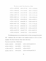
The following answer set was obtained when local time was mapped into global
time. Additional rules were added to the translated program in order to do this
mapping. We will not talk about these rules in this thesis.
% process-name(Value.
Global-time).
out flow-rate(6,0).
volume(25,0).
inflow-rate(changed(0,3),0).
out flow-rate(6,l).
volume(28,l).
inflow-rate(3,l).
outflow-rate(7,2).
volume(31,2).
inflow-rate(3,2).
outflow-rate(7,3).
volume(33,3).
inflow
40
j'ate(changed(3,0),3).
outflow-rate(6,4).
volume(26,4).
inflow.rate(0,4).
outflow-rate(5,5).
volume(20,5).
inflow jrate(0,5).
outflowjrate(4,6).
volume(lb,6).
inflow
outflow-rate(4,7).
volume(ll,7).
inflow jrate(0,7).
outflow-rate(3,8).
volume(7,8).
inflow-rate(0,8).
outflowjrate(2,9).
volume(4,9).
inflow-rate(0,9).
j'ate(0,6).
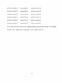
As we can see inflow-rate is not uniquely defined at global time 0 and 3. It changes
from 0 to 3 at global time 0 and from 3 to 0 at global time 3.
41
CHAPTER 5
PLANNING AND DIAGNOSIS
In this chapter we will look at some examples on how to do planning and
diagnosis in a h>-brid domain. The existing theories for planning and diagnosis can
be applied to hybrid domains.
5.1
PLANNING
The ability to plan is an important characteristic of an agent. A plan is a
sequence of actions that satisfies the agent's goal. By goal we mean a finite set of
literals of H the agent wants to make true.
A planning problem can be solved in different ways. Answer set programming
techniques is one of them. In this approach, the answer sets of an A-prolog program
encode possible plans. These plans are generated by so called 'planning modules'
In our examples the planning module is often a simple choice rule. Answer
set planning does not require any specialized planning algorithms. The reasoning
mechanism used for planning is the same as the one used for deducing answer sets.
Let us now look at an example that involves planning.
Example 5.1 Consider a car moving along X-axis with uniform velocity. The domain
consists of two actions start(V)
and stop.
42
start(V)
causes the car to move with
a velocity.
\' a n d stoji causes t h e velocity
continuously with time as long as velocity
to b e 0. position
of tlie car changes
is not, zero.
Let us construct an action description AD-s describing the above domain. T h e corresponding signature E3 contains the actions slarl(V)
position,
a n d fluents velocity,
posilion(0),
and stop, continuous process
a n d posit ion (end).
is t h e set of real numbers and t h e range(position)
The
range(velocity)
is t h e set of non-negative real
n u m b e r s . Let Q3 contain t h e function
a T = 0.
YQ
f,(YQ,\-T)
=
f,(Yo,V,T-l)
where YQ G range(position),
+V
V G range(velocity)
ffT>0.
and T is a variable for time. The
action description .47^3 contains the following statements. The effects of the action
start(V)
where U G range(velocity)
start(V)
wiU given by the causal law:
causes
velocity = V.
which says that performing the action start(V)
(5.1)
at time end in a state s causes velocity
to be V in any successor state of s. The executability condition will have the form:
impossible
start(V)
if
velocity / 0.
which says that in any state, s, it is not possible to perform start(V)
(5.2)
at time end
if the velocity is not zero. In other words, the car cannot be started if it is already
moving. The effects of the action stop will be given by the causal law:
stop causes
velocity = 0.
43
(5.3)
which says that performing the action stop at time end in a. st,a,t,e s causes the velocity
of the car to be 0 in any successor state of .s. The executability condition wiU have
the form:
inil>ossible stop if
velocity = 0.
(5.4)
which sa>-s that in an>' statt\ s, it is not possible to stop the car at time end if the
velocity is 0. In other words, the car cannot be stopped if it is not moving, position
is defined b\' the state constraint
position
= fr,(^'Q,V.T)
If position(0) = YQ,
(5.5)
velocity = V.
which says that position is defined by Newtonian equations in any state.
We will now consider the program aiADs),
obtained by translating the statements
of AD3. The actions and processes of the domain will be declared as
action(start(V),
agent) : —
range{velocity,V),
V >0.
action(stop,
agent).
process(velocity,
fluent).
process(position,
continuous).
Statement (5.1) wiU be translated as
val(V, velocity, 0, 7 + 1) : - o(start(V),
T, I),
range{velocity,
44
V).
Statement (5.2) will be translated as
:-
o(start(\-),T,I),
val{\'0.i-(locily,T,I),
vo ^ 0,
range(velocity,
\''),
range(v(locity,
VO).
Statement (5.3) will be translated as
val(0. velocity. 0, 7 + 1) : --o(stop, T, I).
Statement (5.4) wiU be translated as
:-
o(stop,T,I),
val(0, velocity, T, I).
Statement (5.5) will be translated as
function
val(f5(Y0,V,T),position,T,I)
:-
/5.
val(YO,position,0,I),
val(V, velocity, T, I),
in(T,I),
45
range(position,
YO),
range(velocity,
V).
Now consider the recorded liisti)r\'. Fj
obs{0,
velocity,0,0).
obs(0,po.'<ition.0,0).
These observations say that initially the car is not moving and positioned at 0. The
program n(.l£)3,ri) is obtained by adding Fi to (\(AD:i).
Now suppose that the goal of an agent acting in this domain is to drive to a
certain position on the X-axis and stop there. We will use the rule
goal(T,I)
: — val(8,position.
T, I),
(5.6)
val(0, velocity, T, I).
to say that the goal is to reach position 8 and stop there. To achieve this goal, the
values of I and T must satisfy the rule
success : — goal(T,I).
(5.7)
Failure is not an option. Therefore, we write
: — not success.
(5-8)
The rules (5.6), (5.7), and (5.8) wiU be added to the program a(AD3,ri).
We know
that I takes integer values from some interval [0, n]. This means that we can look for
plans of no more than n consecutive steps. Candidate plans will be generated by the
choice rule, PMQ:
{o(A,T,I)
: action(A,agent)}
46
: -I
<n.
For an\- \'alue of 1 ranging from 0 to /; - 1, if the goa,l is not, satisfied, PMQ wifl select
a candidate action. Pj'l7o is also called the planning
moduli
Answer sets of the program cy(AD-j„Tx) U PM^ wiU (Micode candidate plans,
i.e. possible sequences of actitms that satisf\' success.
In our example, I and T take integer values from the intervals [0,2] and [0,6] respecti\el>-. A total of 21 different candidate plans were generated and the average run
time was 4.6 seconds of which SMODELS took 2.75 sees and Lparse and SMODELS
together took 4.4 seconds. One of the candidate plans
o(s^a/';(2),4,0).
o(stop,4,1).
is to start driving with a velocity of 2 at time point 4 of step 0 and then stop at time
point 4 of step 1 at which point the car is positioned at 8.
5.2
DIAGNOSIS
In this section we are interested in the agent's ability to diagnose. Diagnosis
involves finding possible explanations for discrepancies between agent's predictions
and system's actual behavior.
The algorithms used in [1; 3] to perform diagnostic tasks are based on encoding
agent's knowledge in A-prolog and reducing the agent's task to computing answer sets
of logic programs. We will use a similar approach to do diagnosis in hybrid domains.
47
The first step of an observe-think-act loop of an intelhgent agent is to observe
the world, explain obscn'Nations, and update the knowledge base. We will try to
provide the agent with the reasoning mechanism to exi)lain observations.
We assume that tin- agent is capable of making correct observations, performing actions and remembering the domain history. We also assume that normally the
agent is capable of observing all relevant exogenous actions occurring in its environment.
Now let us look at some terminology. Let D be a diagnostic domain.
Definition 5.1 B\' a diagnostic domain we mean the pair (S, TD) where E is a domain
signature and TD is a transition diagram over E.
Consider an action description, AD of H that describes D. Let F^ be a recorded
history of D up to moment n. Now, consider a mapping a, that maps the domain
description V = {AD, r „ ) into rules of A-Prolog. The resulting logic program will be
denoted by a(AD, r „ ) .
The recorded history, r „ contains a record of all actions, the agent performed
or observed to have happened upto moment n - 1. This knowledge enables the agent
to make predictions about values of processes at the current moment, n.
To test these predictions, the agent observes the current value of some processes. We simply assume that there is a collection, P, of processes which are observable at n. The set
O" = {obs(v,p,t,n)
48
-.peP}
contains the corresponding observations. At this point it is convenient to spht the
domain's history into two parts. Thc> previously recorded history, r „ and the current
ol)ser\-ations (3" A pair
c = (r„.0")
will be often referred to as system's configuration. If new observations are consistent
with the agent's view of the world, i.e. if C is consistent, then O" simply becomes
part of recorded histor.\-. In other words r„+i = C. Otherwise, the agent has to start
seeking the explanation(s) of the mismatch.
Let
conf(C) =
a(AD,Tn)UO''
C is consistent iff conf(C) has an answer set.
Definition 5.2 The configuration C is a symptom
of system's malfunctioning iff the
program conf(C) has no answer set.
An explanation of the symptom can be found by discovering some unobserved past
occurrences of exogenous actions. Let £ denote a set of elementary exogenous actions
corresponding to D.
Definition 5.3 An explanation,
E, of symptom C is a collection of statements
E = {hpd(a, t,i) : 0 < i < n and a e £}
such that r „ U O" U £• is consistent.
49
Answer set programming provides a way of computing explanations for inconsistency
of C. Such a computation c an be viewed as 'planning in the past'
We construct a ])rogram called diagnostic module, DM, tlia,t computes explanations.
The simplest diagnostic module, DMQ. is defiiKnl by the choice rule of SMODELS.
{0(^1, T, 7) : action(A,ex)}
: -0 < I < n.
where e.r stands for exogenous action.
Finding diagnoses of the symptom, C, is reduced to finding answer sets of the
program conf(C) U DMQ. A set E of occurrences of exogenous actions is a possible
explanation of inconsistency- of C iff there is an answer set Q of conf(C) U DMQ such
that
E = {o(A. T, I) : action(A, ex) A o(A, T,I) EQA
hpd(A, T, I)
^Q}.
Let us introduce some faults in Example 4.1 of the water tank and see how a diagnosis
is done when the agent's predictions do not match with reality.
First we introduce the exogenous action 'break' which causes the faucet to
malfunction. By malfunction, we mean that the faucet will be unable to output any
water even when it is open. We will introduce the boolean fluent 'broken' to denote
that the faucet is broken.
We extend the signature, E2 in Example 4.1 to include the exogenous action
break and fluent broken. A few additions and modiflcations wifl be made to the action
description ^7^2 of Example 4.1. The effects of the action break will be given Iw' the
50
causal law:
/)rrr;A' causes
broken.
(,'j.fj)
which says that the exogenous action break causes the faucet to be broken.
The
executability condition is of the form
impossible
break if
broken.
(5.10)
which says that the faucet cannot break if it is already broken.
Statements (5.9) and (5.10) are now part of AD2. The statements (4.9) and (4.10)
wifl be modified to accomodate the effects of break.
in flow.rate
= 3 if
open,
(5-11)
-'broken.
inflow-rate
= 0 if
open,
(5.12)
broken.
Let us now look at the translations of the above statements. First we must declare
the exogenous action break and the fluent broken.
action(break,
process(broken,
ex).
fluent),
broken is a boolean fluent. Therefore, range(broken)
range(broken,
true).
range(broken,
false).
51
is deflned as
Now. a(AD2) from example (4.1) wiU contain the rules (4.13), (4.14), (4.15), (4.16),
(4.18), (4.19), (4.20), and the following rules:
Statement (5.9) is translated as
val{true. brokin.O. 7 + 1) : -o(break, T. I).
Statement (5.10) is translatetl as
:—
o(break,T,I),
val{true. broken, T, I).
Statement (5.11) is translated as
val(3.inflow-rate,T,
I) : — val{true, open,T, I),
val(false,
broken, T, I).
Statement (5.12) is translated as
val(0,inflowjrate,T,I)
:-
val(true,open,T,I),
val(true, broken, T, I).
Example 5.2 Consider the recorded history, Fi containing the observations
hpd(turn(open),
0,0).
obs(false, open, 0,0).
obs(25, volume,
obs(0, inflow-rate,
0,0).
0,0).
obs(false, broken, 0, 0).
52
Let O^ = {obs(0, In floiv-idte,
0,1)}.
obs(0, in ftoii'_nili. 0.1) says that
was observed to be 0 at time 0 of ste]) 1. ()l)\iousl\', v<il{3. iiiflowj-ate,0,1)
rnflow-rate
predicted
l)y Fl contradicts the observations.
This discrepancy can be explained by unobserved occurrence of action break
at time 0 of step 0. We will now see how to compute the possible explanations.
The program conf(C) = o(. 17^2-Pi) U O^ is inconsistent. Therefore, we augment it with the diagnostic module, DM^
{o{A.T,I)
: action(A,ex)}
: -0 < I < n.
The resulting program conf(C) U DMQ is consistent and has an answer set that contains o(break, 0,0) which is the possible explanation for the inconsistency of conf(C).
The average run time for this program was 4.9 seconds of which SMODELS took 2.1
seconds and Lparse and SMODELS together took 4.7 seconds.
Example 5.3 Let us look at another scenario where answer set programming alone
may not be enough to find explanations.
Consider the history, Fi
hpd(turn(close),3,
0).
obs(true, open, 0,0).
obs(25, volume, 0, 0).
obs(3, inflow-rate,
0,0).
obs(false, broken, 0,0).
53
and the new observation, O^ = {obs(n,
volume,0,1)}.
The program conf(C)
=
a(AD2, Fl) U O^ is found to be inconsistent,. So it is augmented with the diagnostic
module D.MQ. The resulting program is stiU hiconsist.ent.
The diagnostic module, DA7o will compute only tli(jse explanations in which
the unobser\ed exogenous actions occur in parallel with agent's action.
In Example 5.3, Fi predicts val(33, volume, 0,1) which contradicts the observation o6s(17. volume, 0,1).
Therefore, we add DMQ to find explanations. DMQ
will look for an exogenous action that occurs at the same time as the agent action
tutn(clo.^e).
But fails to find one.
In reality an unobserved exogenous event must have happened before the
agent action was executed. A possible explanation for the unexpected observation
o6s(17, volume, 0,1) is the unobserved occurrence of break at time 1 of step 0.
Similarly, there may arise situations in which break could have happened at
time point 0 or time point 2 of step 0. DMQ will be unable to explain the unexpected
observations in both situations.
Therefore, answer set programming alone is not enough to do diagnosis in such
situations. We have some ideas on how to approach such problems. But before we
talk about them, there are other issues such as grounding that must be addressed.
In most of our examples agent's knowledge is encoded in A-prolog and inference
engines such as SMODELS are used to reason about such knowledge. Computing
values of processes may involve trignometric functions, differential equations, complex
54
formulas etc. Existing answer set solvers cannot cany out such computations. Also
when numbers l)ecome large, the solvers run out of mcmor\'. Besides this, SMODELS
grounds all xariables in the program leading to poor efficiency.
In the following paragraphs, we propose an ag(-nt architecture for hybrid domains which will overcome computational problems and aid in efficient diagnosis.
A solution to the computation problem is to limit the answer set solver to
reason about effects of actions and leave the computations to an external program.
The external program will be called monitor.
The agent and the monitor will interact
with each other in the following manner.
The agent"s task will be reduced to computing the answer sets of an A-prolog
program. The answer sets will contain information about the values of processes at
time 0 and the functions associated with these processes. The only change is that
these functions are not evaluated yet.
The answer sets will be input to the monitor which then evaluates the functions
asssociated with processes. Each time the agent performs an action the initial values
and functions will be input to the monitor. The monitor will record all occurrences
of agent actions.
The monitor will be capable of observing actions that occur naturally or triggered by other actions in the environment. It wifl report such observations to the
agent. The agent will do the reasoning and send new input to the monitor.
55
An important function of the monitor is to help the agent diagnose.
The
computations done by the monitor will become the predictions of the monitor. The
monitor will record ol)ser\'ations with the help of sensors and then compare these
observations with its predictions. If there is discrepancy it will inform the agent of all
those observations that did not match, along with the time at which the discrepancy
was found.
With this information the agent's task will become easier. Now the agent
already knows when the exogenous action(s) occurred. It still needs to find out what
exogenous action(s) took place
For this the agent will use answer set programming
techniques. Once the correct explanation is found, the agent reasons about the effects
of the exogenous action(s) and sends input to the monitor. The monitor will record
the occurrence of exogenous action(s).
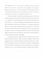
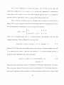
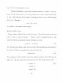
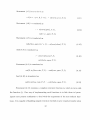
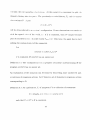
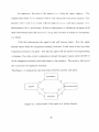
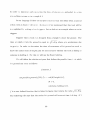
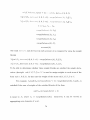
The Figure 5.1 summarizes the interaction between monitor and agent.
actuators
environment
agent
monitor
Figure 5.1: Architecture of an agent in a hybrid domain
56
The labeled arcs denote the following:
1
The agent inputs initial values antl functions associated with processes to the
monitor.
2
Monitor informs the agent about discre])ancies. actions triggered in the environment, initial situation, etc.
3
Monitor observes the environment.
4
Monitor records observations.
5
The agent sends messages to the actuators to perform actions.
6
The actuators perform actions in the environment.
Finally we say that with the help of monitor we will be able to find an explanation
for the inconsistency in Example 5.3, overcome computational problems, and improve
efficiency considerably.
There are still some pending issues such as grounding in
SMODELS which can be overcome by delayed grounding.
Example 5.4 Now let us see an example in which the monitor detects inconsistency
and reports it to the agent and the agent uses answer set programming techniques to
find out an explanation for inconsistenc}'. We will use the water tank example again.
Consider the recorded history, Fi consisting of
57
obs(3, infloivj-nlf,
0, 0).
obs(25, volume. 0.0).
obs{false.broken,0,0).
obs(true.op(ti.0,0).
Suppose that the monitor observes that infloiv.rate
is 0 at time 3 of step 0. But the
predicted \-aliie is 3. Since there is a discrepancy it sends a message to the agent that
in flow-rate
was observed to be 0 at time 3 of step 0. This will be represented by the
fact:
error(0, inflow-rate,
3,0).
(5.13)
Now we write the general rule
obs(Y, P, 0, 7 + 1) : - error(Y, P, T, I).
(5.14)
which states that since an error was detected at time T of step I it must be true that
an exogenous action must have occurred at this time, and therefore Y will be the
observed value of process P at time 0 of the next step, I + l . We also need the rule
end(T, I) : - error(Y, P, T, I).
(5.15)
to make sure that the step ends at time T when the discrepancy was detected.
The maximum number of steps is incremented by one and the rules (5.13), (5.14),
(5.15) are added to the program a(AD2,Ti).
58
The resulting program is inconsistent.
Therefore we augment it with the diagnostic module, DM\ to restore consistency.
{o(A, T, I) : action[A. e.v)} : - error{Y, P, T, I),
(5.16)
I < n.
The answer set of the resulting program contains o(/);'fY;A', 3,0) which is indeed the
correct explanation. The average run time for this program was 4.9 seconds of which
SMODELS took 2.1 sees and Lparse and SMODELS together took 4.6 seconds.
59
CHAPTER 6
RELATED WORK
In this chapter we will compare^ language H with tw<j other languages used
for similar purposes. The first language is called situation calculus [13; 14] and the
second one is called AVC [4] which stands for Actions with I^elayed and Continuous
effects.
6.1
SlTU.-^TION CALCULUS
In this section we will compare language H with situation calculus. Situation
calculus was introduced by John McCarthy in 1963 as a language for representing
actions and their effects. But it was Reiter who enhanced situation calculus with features like time, concurrency, and natural actions to be able to model hybrid systems.
Situation calculus or sitcalc for short uses an approach based on first-order
logic for modeling dynamical systems. The statements of the language are formulas
of first-order logic. We on the other hand , use an action language/logic programming
approach to modeling dynamical systems.
Situation calculus does not use transition function based semantics to characterize actions. By transition function based semantics we mean the approach in
which the world is viewed as a dynamical system represented by a transition diagram
60
whose nodes correspond to possible physical states of the world and whose arcs are
labeled by actions.
Situation calculus uses the term situation to denot.e a possible world history.
A .situation is a finite sequence of actions. An initial situation denotes an empty
sequence of actions.
In [14] Reiter points out the difference between the terms situation and state
as - a state is a snapshot of the world while situation is a finite sequence of actions.
A state is a collection of fluents that hold in a situation. Two states are the same if
the>' assign the same truth values to all the fluents. Two situations are the same iff'
the>- result from the same sequence of actions apphed to the initial situation. Two
situations may be different yet assign the same truth values to the fluents. Situations
do not repeat while states can repeat.
E.g. Consider the blocks world domain. Let move(a,b),
move(c,a)
situation, s, resulting from performing the action move(a,b) followed by
denote a
move(c,a).
A state, st, corresponding to the situation s will contain the fluents on(a,b) and
on(c, a).
Let us talk about some situation calculus terminology. The symbol do(a, s)
denotes a successor situation to s, resulting from performing action a in situation
s. Relations whose truth values vary from situation to situation are called relational
fluents. For example, on(x, y, s) denotes that block x is on y in situation s. Functions
whose values vary from situation to situation are called functional fluents. For exam-
61
pie, height(s)
denotes t,he height of an object in situation s. Since the language is
based on first-order logic, the full set of quantifiers, connectives and logical symbols
are used, making the language powerful and expressive.
But there are some limitations. Situation calculus does not encourage the
use of state constraints because they are a source of deep theoretical and practical
difficulties in modeling dynamical systems. Let us understand why.
We know that the statements of the language are formulas of first-order logic.
A state constraint will be written as .4 D B where A and B are first-order formulas.
The contrapositive -'B D -^A will also be true in this case.
For example, the state constraint
on(x, y, s) A on(x, z,s) D y = z.
expresses a truth about the blocks world domain.
But the contrapositive is not
necessarily true.
y ^ z D -'on(x, y, s) V ^on(x, z, s).
This shows that using classical implication for knowledge representation does
not give expected results. For this and other practical reasons situation calculus does
not encourage the use of state constraints.
In situation calculus, the axioms for representing actions and their effects
presuppose that actions are deterministic.
Therefore, the action theories contain
deterministic actions only. On the other hand, action theories of H contain both
deterministic and non-deterministic actions.
62
Sitcalc requires that the initial situation be complete^. We do not have sudi restrictions for language H. And t lu^ implementation in A-Prolog is capable of handling
incomplete initial situations.
In [14] Reiter introduced the term process in order to overcome the problems
associated with concurrent execution of actions with durations.
Reiter conceives
actions with duration as processes, represented by relational fluents, and introduces
durationless actions that initiate and terminate these processes.
For example, instead of the action walk(x,y) we might have instantaneous actions start\Valk(x,y)
and end\Valk(x.y) and the process of walking from x to y, repre-
sented b>- relational fluent walking(x,y,s).
true, endWalk(x.y)
startWalk(x,y)
causes the fluent to become
causes it to become false. With this device of instantaneous start
and end actions, arbitarily complex concurrency can be represented. For example,
{startWalk(A,
B), startChewGum},
{endChewGum,
startSing},
{endWalk(A,B)}
is the sequence of actions beginning with simultaneously starting to walk and starting
to chew, followed by simultaneouly ending to chew and starting to sing, followed by
ending to walk (at which time the singing process is still going on).
Since we assume that actions of H are instantaneous we adopt Reiter s approach to model actions with durations and delayed effects. The only difference is
that the term process refers to both fluents and continuous processes.
Reiter adds explicit representation for time to situation calculus which allows
63
to specify the exact times, or a range of times, at which actions in a world history
must occur. The temporal argument is added to all instantaneous actions, denoting
the actual time at which an action occurs. For example, bounce(ball,wall,7.3) is the
instantaneous action of ball bouncing on wall at time 7.3. Here time refers to global
time unlike our approach where local time is used.
New function symbols are introduccnl in the language to handle the temporal
argument. A new function symbol time : action -^ reals is introduced, time(a) denotes the time of occurrence of action a. For example,
time(bounce(ball,wall,7.3))=7.3.
Another function symbol start : situation —> reals is introduced,
start(s)
denotes the start time of situation s. Therefore,
start(do{a,s))
=
time(a).
The start time of the initial situation, So is arbitrary and may or may not
be deflned depending on the application. In our approach the initial state starts at
global time 0.
In sitcalc, every action takes time as one of its arguments and every fluent takes
situation as one of its arguments. In our approach, the time and state parameters
are not explicitly mentioned in the statements of H but it is imphed that they are
associated with every action and process.
The value of a fluent with the situation argument s is its value at the start
time of s. For example, the functional fluent height(s)
denotes height at the start
time of s and height(do(a, s)) denotes height at the start time of do(a, s).
64
The language does not provide an\' featurc^s to compute the value of a fluent
at a time other than the start tini(> of a situation. If there is an action that occurs at
every time point then it is possible t.o define fluent values at every time point.
In language H, we have a collection Q of functions for deflning continuous
processes. For instance in example (2.1) from chapter 2 we have functions /o and / j
for defining height.
Let us do an axiom by axiom comparision of situation calculus and H. For this
we wiU model the Example 2.1 from chapter 2 in situation calculus. In that example
we had actions drop and catch and processes holding and height.
The continuous
process height will be treated as a functional fluent, holding will be treated as a
relational fluent.
To reason about the effects of actions situation calculus uses three kinds of
axioms namely action precondition axioms, successor state axioms and unique names
axiom for actions.
Action precondition axioms specify conditions that must be satisfied in order
for an action to be executed in any situation. They can be considered as counterparts
of executability conditions of language H. They are more powerful than executability
conditions in the sense that they can be used to determine the occurrence times of
natural actions. The following example demonstrates how to use action precondition
axioms to predict the occurrence times of a natural action such as bounce.
65
Example 6.1
poss{bouncc(l),.s)
= isFalling{s)
A
{heighl(.s) -\- vvl{s){t - start(s)]
Icit-.start
-
(.s)]' = 0}.
Note that in situation calculus lower case k^ter are used to denote variables and
upper case letters are used to denote constants, height(s)
and vel(s) are the height
and velocit>- of the ball at start of situation s. poss(bounce(t),
s) means that bounce
is physically possible at time / during situation s.
The action precondition axioms for drop and catch from Example 2.2 will be
poss(drop(t),s)
= holding(s) A height(s) / 0.
poss(catch(t),s)
=
-'holding(s).
Successor state axioms define the value of a relational fluent or functional
fluent in the successor situation resulting from performing an action in the current
situation. It has two parts. The first part defines what action causes the fluent to
have a new value in the successor situation. The second part captures inertia. It says
that the fluent will retain its value from the current situation if the action had no
effect on the fluent. Let us define the fluents holding and height from Example 2.2
using successor state axioms of situation calculus.
holding(do(c, s)) = (3t) catch(t) ^ c \/
holding(s) A -^(3t)drop(t)
66
(6-1)
G c.
-'holding(do(c,
s)) = (3t) drop(t) G c V
-^holding(s) A -'(3t)calcli(t)
(6.2)
G c.
height(do(c, s)) = h = holding(s) Ah = hcigiit(s) V
-'holding(s)
(6.3)
Ah = height(.s) - \ G liine(c)'^.
Tlu^ concurrent action c in the above statements is a collection of simple actions that
occur at the same time. As \'ou can see the successor state axiom for a fluent /
provides the dual functionality of a dynamic causal law of H with / in the head and
the inertia axiom for / in a single statement. Note that we use state constraints to
define height in Example 2.1.
Consider the axiom (6.2). Suppose that in the initial situation SQ, holding is
true. Now suppose that action drop occurs at global time 0 causing holding to be
false in the resulting situation Si. This means that holding is false at 0. In other
words, it is uniquely defined at 0. This is possible because the start time of SQ is not
defined.
In our approach we use local time. Suppose that at local time 0 of the initial
state , holding is true. Now suppose that the ball is dropped at this time. This causes
holding to be false at local time 0 of the successor state. Since both these local times
map to the same global time 0, holding is not uniquely defined at 0. Global time 0
is the point of transition for the value of holding from true to
67
false.
Coming to implementation, axioms of situation calculus are translaterl into
rules of Prolog. The resulting program can hv verified for cori-ectness by querying
the prolog interpreter for fluents values and occurrence times of actions. The existing
prolog systems support floating point numbers, thereby allowing fluent values and
occurrence times of actions to be real numbers. Reiter's group uses the Eclipse Prolog
s>-stem primarily because, as implied b>' its name
Programming Sxstem
the ECLiPSe Constraint Logic
provides built in constraint solving libraries that are used for
temporal reasoning.
Most of the existing prolog systems suflcr from floundering, omit 'occurs check'
and are not capable of generating multiple models. Eclipse Prolog overcomes some
problems involving non-ground negative atoms but suffers from other drawbacks.
We translate statements of H into rules of A-Prolog. A-Prolog uses a reasoning
algorithm that is completely different from the one Prolog uses and overcomes many
of Prolog's shortcomings. A-Prolog programs can have multiple models which means
that A-prolog can handle non-determinism. It is also capable of representing defaults.
The task of predicting the values of processes and the occurrence times of
actions is reduced to computing answer sets of A-Prolog programs. We use existing
answer set solvers like SMODELS to compute answer sets of our programs.
Reiter's main goal was to model natural actions- actions that occur in response
to known laws of physics. For example, a ball bouncing on the floor after being
dropped.
The occurrence time of bounce is determined by Newtonian equations.
68
In order to represent such an axtion the laws of physics are embodied in action
prectJiidition axioms as in example 6.1.
In our language H there are no special axioms that will deflne when a natural
action such as bounce will occur. In chaptcn- 2 we mentioned that this task will be
accomplished b\' writing action triggers.
Let us look at an example where we write
triggers.
Suppose that a book was dropped from a height h above the ground. The
time at which it hits the ground is equal to J2 * h/g where g is acceleration due
to gravit>'. In order to determine the time of occurrence of hit-ground
we need to
know the initial value of height plus we need to know whether the book is falhng or
someone is holding it. For this we will use the fluent holding.
We will define the relation act-poss that defines the possible time, t, at which
hit-ground
can occur as follows:
function
act-poss(hit-ground,f(H),l)
f.
: - val(H, height, 0,1),
H >0,
val(false,
holding, 0,1).
/ is a user defined function that is linked to Iparse that returns the value ^ 2 * 77/5.
The following rule says that the action hit-ground
69
will occur at time t of step i if t
is the time at which it is supposed to occur and / is a time point during step /.
o(hit_grounil,T.
I) : — acLposs(hil Jirou.nd,T, I),
in(T,l).
An other approach to modeling natural worlds is to get rid of natural actions
and just ha\'e processes. The eflects of actions will then be captured by process
definitions. This nia\' probabl\' lead to complex process definitions but it gives us
another approach to compare with.
Example 6.2 Let us revisit the Example 2.2 from chapter 2
We will model this
example again but with a diflerent approach. We will get rid of the natural action
bounce.
The action description ADi that we constructed previously will be modified.
Let us call this modified version as AD\. Please note that velocity will be treated as
a continuous process now.
The corresponding signature Ej contains the continuous processes position
and velocity and fluents position(0),
position(end),
velocity (0), velocity (end).
Q\ contains the functions
ff
YQ
T
= 0.
fQ(YQ,VQ,T) = \
foiYQ,VQ,T-l)
+ fi(VQ,YQ,T-l)
70
ffr>0.
lo
^0
/i(Vo,lo,T) =
ffr
= o.
if/o(^i), ^ , 7 " ) 7^ (/'Pi
and
/o(yb, \Q.T) ^ v!p2 and
T>0.
-10
where YQ G range(position),
otherwise.
VQ G range(velocity)
and wpi, wp2 are constants de-
noting the position of the walls u'l and W2 respectively. The process position will be
defined l)y the state constraint
position = /o(yo, VQ, T) if position(0) = YQ,
velocity (0) = VQ.
which says that position will be defined by Newtonian equations in any state, velocity
is defined by the state constraint
velocity = /i(Vo,Vo,r) / / velocity(0) = VQ,
position(0)
= YQ.
which says that the direction of velocity will change only when the position of the
ball is the same as the position of a wall. This is of course when velocity is not zero.
The effects of the action bounce are captured by the function / i .
When we look at Examples 6.2 and 2.2, and the way they are modeled in
H there is not much difference.
The advantage of Example 6.2 is that when we
implement it using A-Prolog, the answer set solver need not compute occurrence
times of bounce.
71
When we implement Example 2.2 we have to write extra rules that will compute the occurrence tunes of bounce. These computations cost us time. The approach
suggested b\' Example 6.2 is just one way of improving efficieiicv
Let us discuss some of the hmitations of H. Language H is not capable of
representing the effects of several concurrently executing actions on a process. We
will use the features of SMODELS to reason about such effects. Let us look at the
following example.
Example 6.3 Consider the actions deposit and withdraw
that effect the balance of
a bank account. Now suppose that multiple deposits and withdrawals
were made
from the same account at the same time. The resulting balance can be computed b}'
adding all the deposits to the existing balance and subtracting all the withdrawals
from it. We will now see how to do this using weight rules of SMODELS.
Let us construct an action description, AD^ of H describing the above domain. The
corresponding signature E4 contains the actions deposit(A, X) and withdraw(A,
X)
which denote depositing X dollars into account A and withdrawing X dollars from
account A respectively and the fluents mcrease(A),
increase(A)
and decrease(A)
decrease(A)
balance(A).
are numerical fluents that denote the increase and de-
crease in account A respectively. The range(balance(A)),
range(decrease(A))
and
range(increase(A))
is the set of real numbers.
The effects of the action deposit(A,X)
deposit(A,X)
will be given by the causal law:
causes
72
increase(A)
= X.
and
which says that depositing A' dollars int,o a,ccount .1 at time end in a st,ate s causes
an increase of A' dollars in account .1 in any successor state of s. It is translated as
i'r(/(A',/7;('/'((;,s'c(.l),(),7 + l) : - o((leposil(A. X).T,
I),
account {A),
rangi (balance (A), X).
The etfects of the action withdraw wifl be given by the causal law:
withdraw(A.
X)
causes
decrease(A) = X.
which is translated as
val(X. decrease(A), 0,7 + 1) : - o(withdraw{A.
X), T, I),
account(A),
range(balance{A).
X).
We cannot deflne balance(A) using our language but we can write the following rules
in the language of SMODELS.
#weight
val(X,P,T,I)=X.
73
val(X. balancc(. 1), 0, 7 + 1) : - rr//( A'„, bal,inn(.\),
A'i[rr//(A';i./;/c;'r(;.sc(.l),0,7 + 1) :
-\2[ral(X^.dccrca.sc(A),0,I
0,1),
rarig({b(il(in.cc{A).X:i)]Xi,
-\- 1) : i-a:nge{balancc(y[), Xi)]X2,
X =
XQ
+ Yi - A'2,
rangc{l)alancc(A),XQ),
range(balance(A),
Xi),
range(balance{A),
X2),
range(balance(A),
X),
account(A).
The total increase and decrease in each account A, is computed by using the weight
literals
A'i[i;a/(A'3, increase(A),
0, 7 + 1) : range(balance(A),
X3)]Xi,
A'2[eo/(A'4, decrease(.4), 0, 7 + 1) : ran^e(6a/ance(A), A'4)]A'2.
To be able to determine whether these weight literals are satisfied the weight declaration 'i^weight
val(X.P,T,I)
= A'.' is used to assign weights to each atom of the
form val{X. P, T, I). In this case the weight of the atom val(X, P, T, I) is X.
For example, A'i[fa/(X3, mcrease(>l), 0,7 + 1) : range(balance(A),X'i)]Xi,
is
satisfied if the sum of weights of the satisfied literals of the form
7;a/(A"3, mcrease(74), 0,7 + 1)
is equal to Ai where A'l G range(balance(A)).
aggregating over elements of a set.
74
Intuitively, it can be viewed as
The new balance is obtained by adding the total increase to the existing
balance and then subtracting the total decrease from it. The rule that, we used to
define balance(,\) is called a weight rule.
An other approach to implementing Example 6.3 is to use ASET-Prolog+ [16]
which is an extension of A-Prolog by sets and aggregates. Functions such as sum
of elements of a set and cardinality
of a set are implemented in this language. The
answer sets of ASET-Prolog+ programs are computed by an inference engine called
the ASET-solver.
Like H, the language of situation calculus is not capable of representing the
effects of several concurrently executing actions on a fluent. Instead sitcalc depends on
the implementation to reason about such effects. Eclipse Prolog has built in aggregate
functions such as sum(L) which returns the sum of elements of list L. sum(L) can be
used to define balance(.{) from Example 6.3.
6.2
LANGUAGE
AVC
The language AVC was introduced by Baral, Son, and Tuan in [4] as a language for specifying actions with durations, continuous effects, delayed effects, and
dependency on non-sharable resources.
^P(^(Actions with Delayed and Continuous eflects) is the flrst language to use
a transition function based approach to dealing with such actions. Language H also
uses a transition function based approach for dealing with such actions.
75
In AVC, actions can have delayed and continuous eflects. This means that
effects of actions might not happen immediately or can last, over a period of time and
therefore actions are associated with time intervals of the form [^1,^2] where t^, is are
real numbers such that, 0 < ij < to.
Example 6.4 The action of driving a car for 10 units of time with velocity v wifl be
represented as drivcQiQ(v).
As mentioned earlier language H adopts Reiter's approach for dealing with actions with durations and delayed effects. For example, the action drive in example 6.4
will be represented b>' the fluent driving and instantaneous actions start-drive{v)
endArive.
start-drive(v)
and
causes driving to be true and end.drive causes driving to
be false.
Since the duration of drive is not captured in our representation, we have to
write a trigger for end-drive which says that end-drive will occur after 10 units of time
since start-drive(v)
was executed. Similarly, sitcalc will need triggers to characterize
actions with fixed durations.
When actions do not have fixed durations, AVC adopts Reiter's approach of
using processes. The start and end actions are treated as instantaneous actions which
initiate and terminate processes.
Let us look at how actions with delayed effects are represented in languages
AVC and H.
76
Example 6.5 Consider a timf> bomb that (-xi)lo(les when the time left on its timer
becomes zero. In language' ADC, we will represent the action of setting a timer to
.r units of time as .sd-tin)cr(.r).
This ;iction causc-s the bomb to explode which is
represented b>' the fluent e.vplosion.
The following proposition of AVC represents
this effect.
set-time r{.v) causes
explosion
from
x to x.
In the above statement, the .r in "x to x" denotes x time units relative to the
time point when setJimer
set-timer(x)
was executed. Therefore, the above causal law says that
causes explosion after exactly x time units since its execution. This
action does not have continuous effects and the only effect is at the x*'' time unit.
This is suggested by the "to x" in the above statement. In AVC, lower case letters
are used to denote variables.
Let us construct an action description AD^ of H describing this example. The corresponding signature Ee contains the actions set-timer(X),
cess time-left
and fluents explosion, time-left(0)
detonate, continuous pro-
and timedeft(end).
explosion is
a boolean fluent; range(timeJeft) is the set of non-negative real numbers. Let Q^
contain the function
f
X
ff
T = 0.
/6(A',T) =
f^(x,T-i)-i
where A' G range(time-left)
ffr>o.
and T is a variable for time. Setting the timer to X
77
time units initializes tiineJeft
to .V. Therefore, we write
s(IJiiner(X)
timeJeft
causes
trtncjcfl(0)
= X.
will be defined by the state constraints
tnncJeft
which says that timeJeft
= f^(X,T)
if
time-left(0)
= X.
wifl decrement with every time unit. The action detonate
will be triggered when timedeft
becomes 0 causing explosion. Therefore, we write
detonate
causes
explosion.
The trigger for detonate will not be part of ADf^.
When we compare both representations, the reader might observe that there
are no time intervals associated with actions of H. Instead the time intervals are
associated with the states of the transition diagram as in Figure 1.2.
AVC contains the following propositions to characterize the effects of actions:
executable
a if
a needs
a causes
a contributes
ci,...,Ck.
ri,...,rm-
f = valf(f, fi,...,
fn,t)
valf(f,fi,...,fn,t)
a initiates
(6.4)
(6-5)
from
ti to ^2.
to f from
p from
78
tg-
ti to ^2-
(6.6)
(6.7)
(6-8)
a It rniinalcs
p al t.,.
(6.9)
/) iSMs.sociated-With
f = valf{f, / i , . . . , / „ , / ) .
p is_as.sociatcd-with
f ^ valf{f. f,,...,
(6.10)
/„,/).
(6.11)
When we compare these propositions with the statements of H, we see that
every proposition except for (6.7) has a counteri)art in H. The executablity conditions
of H are counterparts of the propositions (6.4) and (6.5). The dynamic causal laws
of H, without the preconditions, are counterparts of the propositions (6.6), (6.8) and
(6.9).
Propositions (6.10) and (6.11) contain functions for evaluating / . The state
constraints of H with empt\' bodies can be viewed as counterparts of these propositions. For example, height = / o ( 5 0 , r ) . The version of AVC presented in [4] does
have conditional effects and state constraints.
The proposition (6.7) affects the value of / at ^i by contributing an increase
specified by valf(f, fi,...,fn,t)
during the interval [^1,^2]. Let us look at an example
from [4].
Example 6.6 Suppose that driving a car with velocity v for 10 units of time consumes
c(v) units of gasoline per unit time. This is expressed as:
driveojQ(v)
contributes
- c(v) * t to gas-in-tank
from
0 to 10.
And suppose that filling gas for 10 units of time will increase the amount of gasoline
79
by 2 * t. This is exinesscnl as:
filLgasQiQ
contribules
2 * / to gas-inJank
fioinO
to 10.
Let us assume that while driving we can refiU and that initially the gas-inJank
was
20. Suppose that action drivei^io(3) starts its (Execution at time 0 and filLgasQ^io
starts it execution at time 0. Let r(3) = 1.5. The net value oi gas-inJtank
at time 1
wifl be = 20 - 1.5 * 1 + 2 * 1 which is 20.5. Similarly at time 2, gas-inJank
= 21 and
so on.
.\s mentioned earlier, language H and sitcalc depend on the implementation to
represent the effects of several concurrently executing actions. Note that properties
of objects that change continuously with time are still referred to as fluents in the
language of AVC.
We will now discuss the semantics for action theories in AVC. In the presence
of time and delayed effects, the effects of an action might not happen immediately
or might last over a time interval. Therefore, a state encodes not only the fluent
values but also obligations due to delayed effects of recent actions and actions under
execution.
A state is a pair (7, Q) where I is an interpretation and Q is a set of future
effects.
An interpretation I maps a fluent / to a value v G dom(f).
Given that
a i , . . . ,a„ are executable in a state s, a function $(s, {(ai, ( i ) , . . . , (a„, f„)},i), where
tl < t2 • • • < in < t, expresses the state of the world after t units of time from the time
^0 corresponding to s assuming that the actions a i , . . . , a„ were started at relative (to
80
^o) limes ti,
/„ r(>spcH't,i\'elv. Note that t is a number > 0. If the effects of the
actions a i , . . . , a „ terminate at a time, t' such that /' < / then the values of fluent.s
during (t'.t] will be defined by inertia.
In ADC, all notions of time are relative. In sitcalc, time is the actual occurrence
time of an action. In our approach, time is local. But it is possible to predict global
\alues of processes b\' mapping local time into global time.
The version of AVC presented in [4] does not allow conditional effects and
temporal preconditions. Examples such as 2.2 in which the effects of actions depend
on the \'alue of some fluents temporally and conditionally, cannot be modeled using
this version of AVC. It does not contain state constraints and therefore will be unable
to model examples such as 4.1.
The authors of [4] are planning to enhance AVC by adding new features such as
those for expressing temporal preconditions, conditional effects, or state constraints.
They use a Java planner to implement their action theories. Results are satisfactory.
81
CHAPTER 7
CONCLUSIONS AND FUTURE WORK
In this thesis we introduced the action language H for modeling hybrid domains.
We looked at many examples and showed how they are modeled in this
language. The s\ntax and semantics of the language were defined. We implemented
action theories of H using A-Prolog. Some examples involved planning and diagnosis.
We were able to show tliat language H overcomes many of the limitations of
sitcalc and AVC.
It provides almost all the functionalities of sitcalc and AVC and
can model domains that cannot be modeled by the other two.
Using local time not only improves efficiency but also allows us to represent
different kinds of time units. For instance, given a transition diagram, TD, the local
time of a state, s G TD, could represent time in the order of seconds, while the local
time of an other state could represent minutes or hours.
For example, consider the action set-timer(X)
that sets the timer on a mi-
crowave to A' time units. The local time of a state resulting from performing this
action represents either minutes or seconds, depending on whether A' is minutes or
seconds.
Now let us look at some future work prospects. One area for future research
is delayed grounding.
By delayed grounding we mean that functional values and
82
timc\s are grounded if and only when needed. This could reduce the program size and
impro\'e efficiency.
.Another area for future research is developing mechanisms for (4ficient planning
and diagnosis. In chapter 5. there were some scenarios where a diagnosis could not
be found. We had some ideas on how to do a diagnosis in such circumstances. One
of the them was to introduce an external program called monitor that would interact
with the A-Prolog programs, do most of the computations, and help in diagnosis. We
would like to pursue this idea in the future.
H>-brid systems often involve control. An agent acting in such a system should
be reactive and deliberative. A reactive agent is one that acts with respect to its sensor
data. A deliberati\'e agent is one that acts with respect to its goals.
Example of a system that combines reactive and dehberative reasoning is the
Mars rover. If the Mars rover finds a rock that is interesting, it would come up with
a plan to reach the rock, and execute it. Hence it is deliberative in this case. On
its way to the rock it may come across obstacles. The system converts its sensory
data to motion vectors to avoid obstacles. Hence it is reactive in this case. Sometimes it replans depending on the sensor data in which case it combines reactive and
deliberative reasoning.
In this thesis we have not addressed how to combine reactive and deliberative
reasoning. We would like to address this issue in the future.
83
REFERENCES
1. M. Balduccini and M. Gelfond. Diagnostic rea.soning with A-Prolog. In Journal
of Theory and Pmctivc of Logic Programming (TPLP), 3(4-5):42.5-461, Jul 2003.
2. M. Balduccini and M. Gelfond. Logic Programs with Consistency-Restoring
Rules. In .L4^7 Spring 2003 Symposium, 2003.
3. C. Baral and M. Gelfond. Reasoning agents in dynamic domains. In Minker,
J. ed., Logic-Based AI, Kluwer Academic publishers, (2000), 257-279.
4. C. Baral, T. Son and L. Tuan. A transition function based characterization of
actions with dela>-ed and continuous eflects. In Proceedings of KR'02, pages
29L302.
5. M. Gelfond and V. Lifschitz. The stable model semantics for logic programming.
In Logic Programming: Proceedings of the Fifth International Conference and
Symposium, 1988, pp. 1070-1080.
6. M. Gelfond and V Lifschitz. Action Languages. In Electronic Transactions on
Artificial Intelligence, 3(6), 1998.
7. M. Gelfond and R. Watson. On Methodology of Representing Knowledge in
Dynamic Domains. In Proceedings of the 1998 ARO/ONR/NSF/DARPA
Monterey Workshop on Engineering Automation for Computer Based Systems, pp.
57-66, 1999.
8. V Lifschitz, Two components of an action language. In Annals of Mathematics
and Aitificud Intelligence, Vol. 21, 1997, pp. 305-320.
9. V. Lifschitz. Action languages, Answer Sets and planning. In The Logic Programming Paradigm: a 25 year perspective, 357-373, Springer Verlag, 1999.
84
10. Norman McCain and Hudson Turner. A < ausai theory of ramifications and
qualifications. In Proceedings of lJCAI-95, pages 1978-1984. 1995.
11. Norman McCain and Hudson Turner. Causal theories of action and change. In
Proceedings of AAAl-97, pages 4(i()-465, 1997.
12. I. Niemela and P Simons. Smodels an implementation of the stable model
and well founded semantics for normal logic programs. In Proceedings of LPNMR '97, pages 420-429, 1997.
13. R. Reiter. Natural actions, concurrency and continuous time in the situation
calculus. In Principles of Knowledge Representation and Reasoning: Proceedings of the Fifth International Conference (KR'96), pages 2-13, Cambridge,
Massachusetts, U.S.A., November 1996.
14. R. Reiter. Time, concurrency and processes. In Knowledge in action: Logical
Foundations for Specifying and Implementing Dynamical Systems, pages 149183, ISBN 0-262-18218-1, MIT, 2001.
15. Richard W^atson and Sandeep Chintabathina. Modeling hybrid systems in action languages. In Proceedings of the 2nd International ASP'03 Workshop,
pages 356-370, Messina, Sicily, Italy, September 2003.
16. Mary Heidt. Developing an inference engine for ASET-Prolog. Master's
University of Texas at El Paso, Dec 2001.
85
Thesis,
APPENDIX A
IMPLEMENTATION OF WATER TANK EXAMPLE
A-Prolog code for implementing the water tank example 4.1 from chapter 4.
% Declarations
% actions
action(tum(open), agent).
action(tum(close),agent).
% processes
process (open, fluent).
process (inflow.rate, fluent).
process(outflow-rate,continuous).
process (volume, continuous).
% time
const m=6.
time(0..m).
#domain
time(T;Tl;T2).
% step
const n=2.
step(0..n).
#domain step (I)% Range of processes
86
range(opcii.truc).
ratige(opcii.false).
raiige(viflow-rulc.O).
rangc(mflow-rate,3).
valucs(0..60).
% Suppose that the maximum volume of the tank
% whose length is 4 m , breadth is 3 m and height is
% 5 m is 60 cubic meter.
range(volume,Y)
:- values(Y).
% The maximum value of outflow_rate is 10.
range(outflow-rate,Y]
:-
values[Y),
Y <= 10.
% Domain independent axioms
% A process cannot have two values at the same time.
-val(Y2,PN,T,I)
.- val{Yl,PN,T,
neq(Y2,Yl),
process(PN,PT),
range(PN,Yl),
range(PN,Y2).
% Axioms for defining 'end' of a state.
I),
cnd{T.I) :-
o(AX,T,l).
action{AX.AT).
% If no action occurs during a step then the step will
% end at the last possible time unit.
{end{m,I)}l.
% No state can have more than one end.
.-
end{Tl,I),
end(T2.I),
neq(Tl,T2).
% Ever\- state must end.
ends(I) :- end(T,I).
;- not ends (I).
% Axioms that define 'in' and 'out'.
out(T,I)
:-
end(Tl,I),
T>T1.
in(T,I)
:- not
out(T,I).
% The value of fluent does not change with time.
88
val{Y,PX,T,I)
:- val() ,
PX,0,1),
in{T,I),
pr()Ccss{PN.
flurnl),
rangc(PN,)').
% Inertia axiom: "Things normally stay as they are."
val[Y.PX,0,I
+ 1) :- val(Y,
PN.T,1),
end{T.I),
not -val(Y.PN,0,I
process(PX,
+ 1),
FT),
range(PN,Y).
% Reahty Check (obs(Val,Process,T,I))
.•-
obs(Y,PX,T,I),
notval{Y,PN,T,I),
process(PN,PT),
range(PN,Y).
o(AN,T,l)
:-
hpd(AN,T,I),
action(AN,AT).
% Axiom for defining initial state.
89
val (YPN,0,0)
:- obs{Y. FN
,0,0),
procc.s.s(PN,PT),
range(PN,Y).
% Process definitions
% 1. open
% D>-namic causal law describing (>fl'ects of 'turn(open)'
val{true.open,0,l
-^ 1) :-
o(turn(open),T,I).
% Executability conditions for 'turn(open)'
.•-
o(turn(open),T,I).
val (true, open, T. I).
% Dynamic causal law describing effects of 'turn(close)'
val(false,
open, 0,7 + 1) .-- o(turn(close),T,
I).
% Executability conditions for 'turn(close)'
;-
o(turn(close),T,I),
val(false,
open, T, I).
% 2. inflow_rate
% State constraints deflning 'inflow_rate'
% If the faucet is open , inflow is 3.
val(3,inflow-rate,T,I)
:-
val(true,open,T,I).
90
% If the faucet is closed, inflow is 0.
val(0,inflowj'ale,T,l)
:- val(falsc.opcn.T,
I).
% 3. outflow_i'ate
% State constraints defining 'outflow_rate'
% outflow_rate is a function of the water level of the tank
function
/4'
val(f-l'('^').outflow-ratc,T,I)
:-
val(Y,volume,T,I),
range (volume
,Y).
% 4. volume
% State constraints defining 'volume'
function
/3'
val(f3'(Y0.X),volume,T+l,I)
:-
val{YO,volume,T,I),
val(N, inflow-rate,
T, I),
m(r + l,7),
range(volume,
YO),
range(in flow-rate,
91
N).
% History
obs[25. volume, 0, 0).
obs(fa!se. open. 0, (I).
hpd(turn{opcn),0.
0).
hpd(turn(closc),3,1).
% Defining some relations to get better looking output.
volumc{Y,T,I)
:- val{}', volume, T, I),
range(volume,
outflow.ratt
[Y.T.I)
:-
Y).
val(Y.outflow-rate,T,I),
range(out flow-rate,
inflow-rate{YT,I)
:-
Y).
val(Y,inflow-rate,T,I),
range(in flow -rate, Y).
% SMODELS directives to hide and show relations.
hide.
show
inflow-rate(Y,T.
volume(Y,T,
outflow-rate(Y,
I),
I),
T, I).
92
PERMISSION TO COPY
In presenting this thesis in partial fulfilhnent of the requirements for a master's
degree at Texas Tech University or Texas Tech University Health Sciences Center, I
agree that the Library and my major department shall make it freely available for
research purposes. Permission to copy this thesis for scholarly purposes may be
granted by the Director of the Library or my major professor. It is understood that any
copying or publication of this thesis for financial gain shall not be allowed without my
further written permission and that any user may be liable for copyright infringement.
Agree (Permission is granted.)
Student Signatuire
Date
Disagree (Permission is not granted.)
Smdent Signamre
Date