Download Optimization-Based Network Planning Tools in Telenor During the

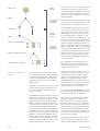
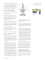
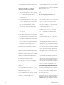
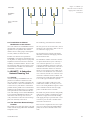
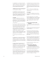
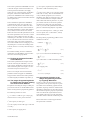
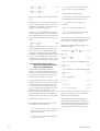
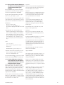
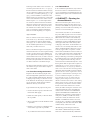
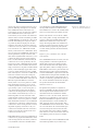
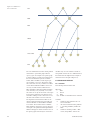
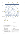
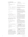
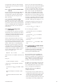
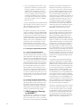
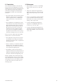
Optimization-Based Network Planning Tools
in Telenor During the Last 15 Years
– A Survey
RALPH LORENTZEN
1 Introduction
Ralph Lorentzen (67) is daily
leader of the company
Lorentzen LP Service which
does consulting work within
mathematical programming. He
retired July 1, 2003 from his job
as senior scientist in Telenor
R&D. Ralph Lorentzen graduated in mathematics at the University of Oslo, where he
worked for some time as assistant professor giving lectures in
statistics and operations
research. He worked as distribution planner in Norske Esso, as
principal scientist at Shape
Technical Centre, as systems
engineer in IBM, and as chief
consultant in Control Data Norway, before joining Telenor R&D
in 1985.
[email protected]
The rapid technological development in the
telecommunications field during the last two
decades made it necessary for the operators to
repeatedly reevaluate the structure, design and
application of their networks. In order to establish cost-effective network design and utilization
many telecommunication operators developed
and used optimization-based network planning
tools. This happened also in Telenor. The rationale was that the frequent technological shifts
did not give the planners sufficient time to
acquire an intuitive feeling of what constituted
good network designs. So the requirement for
comprehensive, cost-effective and robust
designs excluded simple back of the envelope
or spread sheet calculations. The idea was that
mathematical models could be used to optimize
network structures and thus contribute to reduce
costs, ensure network reliability and improve
operational efficiency.
The approach was said to be pragmatic but thorough; heuristic but nevertheless intelligent. The
aim was not to give a black box answer, but a
deeper understanding of the issues and of the
consequences of proposed solutions. The optimization tools were not meant to give a final
answer, but to constitute instruments to be integrated into the decision process of the planners.
Common to all the tools were that they were
based on mathematical programming. The different network components were modeled as
decision variables with associated costs. Technological constraints were modeled by equations
and inequalities that the decision variables had
to satisfy. Commercially available optimization
software together with tailor-made program
modules were used to find cost-effective solutions. The fact that the tools were to be used by
others than the ones who developed them implied that they had to be incorporated in high
quality user interfaces and linked up to relevant
data sources in an appropriate way. In general
the effort spent on the development of user interfaces exceeded the effort spent on implementation of optimization algorithms by a factor of
three to four.
In 1986 Telenor R&D together with the consultant company Veritas established a group of
three people who started building optimization
models for key network design problems.
Telenor R&D was mainly responsible for the
Telektronikk 3/4.2003
modelling whilst Veritas was given the task of
implementing the models. Later on the consultants at Veritas moved to the consultant company Computas, and the cooperation with Computas has continued to this day.
From the outset a good cooperation was established with network operators in the field who
allocated time and energy to specification and
testing.
The initiative was triggered by a situation where
a local cable TV network planner compared two
alternative network layouts which both seemed
reasonable, but discovered afterwards that the
cost of one of the layouts was twice the cost of
the other. The group worked together on and off
over a period of about 15 years and designed and
implemented a series of network planning tools
based on integer programming. Some of the
tools will be described in the sequel, namely
KABINETT, ABONETT, FABONETT,
PETRA, MOBANETT, and MOBINETT.
2 KABINETT – A Cable TV Network Planning Tool
2.1 General
At the time when the cable TV network planning
tool KABINETT was developed the networks
should have a tree structure. Manual planning
was time-consuming, and the planners had
capacity for analyzing a few alternatives only.
One important feature of the planning problem
was to secure that the subscribers received sufficient voltage with a minimum number of amplifiers. Also, the cost of civil work constituted a
large portion of the total cost. Of course, the
planning problem became much simpler later
when the decision was made to go for star networks in lieu of tree networks.
2.2 The Cable TV Network Design
Problem
Here will be given a short description of the
cable TV network design problem KABINETT
attempted to solve.
We were given a signal source and a set of subscribers. The signal source was to be connected
to the subscribers by copper cables via amplifiers, splitters and taps.
The amplifiers, splitters and taps had to be
placed in cabinets. There were two types of cabi-
47
Signal source
D1/D2
network
Splitter
(no attenuation
calculations
performed)
D3 amplifier
Splitter
D3 and
subscriber
network
Transit tap with subscribers
(attenuation
calculations
performed)
Splitter (possible, but unusual)
nets, large cabinets and small cabinets. Amplifiers must be placed in large cabinets while splitters and taps could be placed in small cabinets.
A cabinet could (in addition to the amplifier in
large cabinets) contain an arbitrary number of
splitters and taps.
The cables were placed in trenches. The trenches
formed a network which was called the trench
network. The trench network was assumed to
have a tree structure.
In KABINETT the signal passed via exactly one
amplifier on its way from the source to the subscriber. These amplifiers were called D3 amplifiers and were placed in the network by KABINETT such that the signal that the subscribers
received had sufficient voltage. In reality it could
be necessary to place additional amplifiers between the signal source and the D3 amplifiers. In
KABINETT there was no voltage calculation on
the stretch between the signal source and the D3
amplifiers. Consequently KABINETT did not
make any analysis of the requirement for amplifiers in addition to the D3 amplifiers. However,
once the D3 amplifiers had been placed, this was
generally straightforward. The users were
48
From the signal source the signal might go via splitters on its way to the amplifiers. This part of the
network will here be called the D1/D2 network.
From an amplifier the signal could go via splitters on its way to the taps. There were two types
of taps, namely terminal taps and transit taps.
Terminal taps had subscriber ports from which
the signal could only proceed directly to subscribers. A transit tap had an additional port, the
D3 port, from which the signal could proceed to
a splitter or to another tap. Normally the D3 port
would be connected to another tap and not to a
splitter. A subnetwork connecting a D3 amplifier
to the taps underneath it will here be called a D3
network. If the D3 amplifier had sufficient voltage to support its associated taps with their subscribers, the D3 network was said to be feasible.
Otherwise it was said to be infeasible. All the
D3 networks that KABINETT proposed had of
course to be feasible.
Every subscriber was connected directly to a
subscriber port on a tap. The subnetwork connecting the subscribers to the taps will here be
called the subscriber network.
Termianl tap with subscribers
Figure 2.1 Possible network
structure
assumed to have access to a calculation program
(which did not perform any optimization) for
voltage and attenuation calculations between the
signal source and the D3 amplifiers, which they
could use as an aid for deciding where to place
additional amplifiers.
Based on the location of the signal source, costs
and locations of candidate trenches, costs and
candidate locations of D3 amplifiers, splitters
and taps, costs and attenuations of candidate
cable types, and subscriber voltage requirements, KABINETT tried to find the least costly
network design. The user could specify parts of
the design and leave it to KABINETT to complete the design at the lowest possible cost.
The algorithms used in KABINETT were heuristic, so a theoretically optimal solution to the network design problem was not guaranteed.
Figure 2.1 shows a possible network structure.
The splitters could have more than two exit
ports, and the exit ports could have different
attenuations. There were also in general many
types of taps where each tap type was characterized by its number of exit ports and the attenuation associated with each individual exit port.
One could have several splitters and transit taps
in series, but normally the signal would not proceed from a tap to a splitter.
Ideally the trench network, the D1/D2 network,
the D3 networks and the subscriber network
shold be optimized together. Instead a separate
Telektronikk 3/4.2003
cost minimization of the trench network was
done first. Then an optimization of the subscriber network was done followed by the optimization of the D3 networks, and finally the
D1/D2 network was determined. The separate
optimization of the trench network was partly
justified by the fact that usually well above 70 %
of the total network cost was the cost of trenches.
2.3 Input
The input to KABINETT specified
• the location of the subscribers to be connected
to the network
• the location of the signal source node
• the location of the nodes where D3 amplifiers,
splitters and taps could be placed
• trench route alternatives
• cable types
• splitter types
• tap types
• the D3 amplifier type
• cabinet types
The trench routes consisted of trench sections,
each of which was characterized by geographical
location, length, and cost per metre.
The cable types were characterized by attenuation and cost per metre.
The splitter types were characterized by the
number of ports and the attenuation at each individual port.
The tap types were characterized by the number
of ports and the attenuation at each individual
port and whether they were transit taps or terminal taps.
KABINETT operated with one type of D3
amplifier which was characterized by cost and
the voltage at the exit port.
There were two cabinet types, namely large and
small. Each type was characterized by cost.
The output could be fed into an interactive calculation program (not described here) for placement of amplifiers in the D1/D2 network. This
program also gave a schematic description of the
solution.
2.5 Determining the Trench Network
The trench network cost minimization problem
is an example of the classical Steiner problem
in undirected graphs. A network of candidate
trenches was given, and the problem was to find
the cheapest possible subnetwork (which must
necessarily be a tree) which connected a subset
of nodes. The nodes to be connected included
the signal source node and the subscriber nodes.
In addition the planner could include amongst
the special nodes some of the equipment nodes,
i.e. candidate nodes for placement of D3 amplifiers, splitters and/or taps.
There could be subscribers who were connected
to the rest of the candidate trench network by
two or more candidate trenches. However, one
might want to avoid using these candidate
trenches for transit cables to other subscribers.
This was achieved by multiplying the cost of
these trenches by a large number before the optimization.
In KABINETT an approximate solution to the
Steiner problem was found using RaywardSmith’s algorithm [1].
2.6 Determining the Subscriber
Network
The model used for the subscriber network was
a classical capacitated plant location model.
The subscribers were to be connected to taps by
cables. In this module all taps were considered
to be terminal taps. One cable type only was
considered for each subscriber. In practice the
planner would assume a default cable type for
all subscribers in an initial run. As a result of inspecting the initial solution he could change the
cable type for some of the subscribers and run
the optimization again.
2.4 Output
The output from KABINETT described the proposed solution to the cable TV network design
problem. It showed
• the trenches to be dug
• what types of cables should be used where
• where D3 amplifiers should be placed
• what type of splitters and taps should be
placed where
• which subscribers should be connected to
which ports on which taps
• a table showing labour costs and bill of materials
Telektronikk 3/4.2003
Each candidate tap was given a cost which was
the sum of the tap cost, the cost of a small cabinet, and the cost of the copper cable needed to
connect the tap to the closest equipment node
in the direction of the signal source node.
The cost of connecting a given subscriber to a
tap in a given equipment node was set to the sum
of the material and labour cost associated with
connecting them with the appropriate cable.
Attenuation was not considered in the subscriber
network optimization. Voltage and attenuation
49
considerations were postponed to the D3 network optimization.
The subscriber network optimization model is
described in mathematical terms below.
The following notation is used:
Subscripts
n denotes equipment nodes,
s denotes subscribers,
t denotes terminal tap types.
Costs
cns denotes the cost of connecting subscriber s to
equipment node n;
cnt denotes the cost of placing a terminal tap of
type t in equipment node n. This cost is the sum
of the tap cost and the cost of a cable from the
tap to the nearest equipment node on the route to
the signal source node.
Capacities
pt denotes the number of subscriber ports on a
tap of type t.
Variables
xns = 1 if subscriber s should be connected to a
tap in equipment node n, and = 0 otherwise.
ynt = 1 if a tap of type t should be placed in
equipment node n, and = 0 otherwise.
Using this notation the optimization problem can
be formulated as follows:
minimize Σnscnsxns + Σntcntynt
2.7.1 General
The method for determining the D3 networks
consisted of three algorithms, namely the construction algorithm, the partitioning algorithm
and the move/exchange algorithm.
Typically, KABINETT started with attempting
to cover all the taps with one D3 amplifier. If
this failed, two D3 amplifiers were tried, etc. If
the minimum number of D3 amplifiers which
KABINETT found was needed was K, and the
parameter ‘extra’ was set to a positive integer,
then KABINETT tried to find the least expensive solution with K, K + 1, …, or K + extra
amplifiers.
The construction algorithm took as input a subset of the taps with their voltage requirements
and placed a D3 amplifier in a node such that
either a feasible D3 network was formed or an
(infeasible) D3 network was formed where the
voltage requirement in the D3 amplifier node
was as low as possible.
The partitioning algorithm was a one pass algorithm for partitioning the taps into a specified
number of subsets and constructing a (feasible
or infeasible) D3 network for each of the subsets.
The move/exchange algorithm was an iterative
algorithm which tried to improve on the solution
found by the partitioning algorithm. The move/
exchange algorithm tried first of all to make an
infeasible solution feasible, and tried thereafter
to find a solution with reduced cost.
Before we treat these algorithms we will
describe the splap concept.
(2.1)
subject to
Σnxns = 1
(2.2)
Σsxns ″ Σtptynt
(2.3)
xns ″ Σtynt
(2.4)
where xns and ynt are 0 – 1 variables.
This optimization problem was solved using a
conventional branch and bound code.
The planner could preset part of the solution by
fixing some of the xns or ynt variables to 1.
When the subscriber network was determined,
the voltage requirement at the taps were calculated and recorded.
50
2.7 Determining the D3 Network
2.7.2 Splaps
In the D3 network KABINETT could place
more than one splitter and/or tap in an equipment node. The result was a collection of splitters and taps which could be characterized by its
total cost, a set of D3 ports with their individual
attenuations, and a set of subscriber ports with
their individual attenuations. Such a collection
of splitters and taps in a node was in KABINETT denoted a splap (see Figure 2.2).
Before the D3 network optimization was started
KABINETT compiled a list of candidate splaps
based on the splitter and tap types in the input.
As mentioned earlier the D3 port of a transit tap
would normally be connected to another tap and
not to a splitter, and the splap list was based on
collections of splitters and taps where this was
the case. The planner decided the size of this list
by specifying the maximal number of subscriber
and D3 ports of the splaps.
Telektronikk 3/4.2003
A splap S was said to be inferior to another splap
S’ if the numbers of subscriber and D3 ports of S
were less or equal to the corresponding numbers
for S’, and the attenuations of the ports of S were
greater or equal to corresponding ports of S’.
The splap list would not contain any splap which
was inferior to another splap on the list.
Figure 2.2 Transformation of
a collection of splitters and
taps in a node to a splap
Splap
2.7.3 The Construction Algorithm
First an outline of the algorithm will be given:
Initially the signal source node was used as what
is called an attraction node.
The voltage requirements in the nodes in the
trench tree were calculated starting from the
taps and proceeding towards the attraction node.
Whenever a junction node in the tree was
reached a splap which minimized the voltage
requirement was placed.
If a node was reached where the voltage requirement was greater than the output voltage of the
D3 amplifier, this node was made the attraction
node the first time this happened. All subsequent
voltage calculations were then made proceeding
towards the new attraction node.
Based on criteria to be detailed below a D3
amplifier was then placed in the vicinity of the
attraction node such that a (feasible or not feasible) D3 network was formed.
The algorithm is described in more detail below.
Algorithm for constructing a candidate D3
network for a subset of taps:
1 Initialize the attraction node to be the signal
source node, label all edges in the trench tree
as untreated, label all the taps as treated and
label the remaining nodes in the trench tree as
untreated. The treated nodes are characterized
by the fact that their voltage requirement is
established.
2 If all nodes are treated, go to 4. Otherwise,
find an untreated node n which is farthest
away from the attraction node. Pick an untreated edge connecting n to a treated node,
calculate and save the contribution to the voltage requirement of n caused by this node (i.e.
the voltage requirement of the treated node
plus the attenuation in a cable between n and
the treated node), and label the edge as
treated. Repeat until all the edges coming into
n from treated nodes are treated. If then there
is only one treated node adjacent to n, set the
voltage requirement in n equal to the contribution to the voltage requirement of n caused
by this node. Otherwise, place in n a feasible
splap which minimizes the voltage require-
Telektronikk 3/4.2003
Subscriber
ports
D3 ports
ment of n, and establish this as the voltage
requirement of n. In both cases label node n
as treated. Go to 3.
3 The first time a voltage requirement of a node
is calculated which exceeds the voltage delivered by a D3 amplifier, change the attraction
node from the signal source node to this node.
Go to 2.
4 If the voltage requirement of the attraction
node does not exceed the voltage delivered by
a D3 amplifier (i.e. the attraction node has not
been changed from the signal source node),
place a D3 amplifier in the signal source node
and terminate the algorithm. Otherwise, try
iteratively to place a D3 amplifier in nodes
obtained by fanning out from the attraction
node until either a node is found whose voltage requirement does not exceed the voltage
delivered by a D3 amplifier or a local minimum of the voltage requirement is found
(which is larger than the voltage delivered by
a D3 amplifier). In both cases a D3 amplifier
is placed in the node found.
If the voltage requirement of the node where the
D3 amplifier was placed exceeded the voltage
delivered by a D3 amplifier, the resulting D3
network was infeasible. In that case the infeasibility was defined to be equal to the difference
between the voltage requirement and the D3
amplifier voltage. If the D3 network was feasible, the infeasibility was defined to be 0.
2.7.4 The Partitioning Algorithm
In KABINETT several variants of the partitioning algorithm were implemented. Here, however, only one of these variants will be described.
The partitioning algorithm took as input a positive integer K which represented the number of
D3 networks.
51
A description of the partitioning algorithm follows.
Partitioning algorithm for creating K
(feasible or infeasible) D3 networks:
1 Start with all the K networks empty. Select the
K taps which are farthest apart, i.e. the K taps
t1, …, tK which maximize mini<j d(ti, tj).
Include one of these taps in each of the K
networks. Go to 2.
2 For each network find its close node, i.e. the
closest node which has not been included in
any of the networks. If none of the networks
have a close node, terminate (every node belongs to a network). Otherwise, order the
close nodes in a list according to how close
they are to their associated network. Label
all the close nodes as untreated. Go to 3.
3 If there are no untreated nodes, go to 5. Otherwise, go to 4.
4 Pick the first untreated close node on the list.
If this close node does not contain a tap, include the node in its associated network, and
go to 2. If the close node contains a tap and
the node can be included in its associated network without making the network infeasible
(this is checked by the construction algorithm),
make this inclusion and go to 2. Otherwise,
label the close node as treated and go to 3.
5 Include the first close node on the list and
go to 2.
2.7.5 The Move/Exchange Algorithm
When a solution was found by the partitioning
algorithm, it was natural to try to improve on it.
Whether the solution is feasible or not, attempts
were made to change it into a feasible solution
with the same number of D3 amplifiers, and
with the lowest cost possible. This was the function of the move/exchange algorithm.
In the description of the move/exchange algorithm the following concepts will be used:
Let N1 and N2 denote D3 networks and let t
denote a tap.
If N2 is infeasible with t in N1, let r1(t, N1, N2)
denote the reduction in the sum of infeasibilities
obtained by moving t to N2.
If N1 is feasible with t in N1, and if N2 is feasible
after t is moved to N2, let rC(t, N1, N2) denote the
reduction in cost obtained by moving t.
52
If N1 is infeasible with t in N1 or if N2 is infeasible after t is moved to N2, let rV(t, N1, N2) denote
the reduction in the sum of voltage requirements
obtained by moving t to N2.
Now we can describe the move/exchange algorithm.
Move/exchange algorithm between a
collection of D3 networks:
1 If all networks are feasible, go to 2. Otherwise, calculate r = max r1(t, N1, N2) where the
maximization is done over all N1, N2 and t in
N1. If r > 0, make a move which gives the
infeasibility reduction r. Repeat until either all
networks are feasible or r ″ 0. If all networks
are feasible, go to 2. If r ″ 0 and 3 has been
executed – stop, otherwise, go to 3.
2 Calculate r = max rC(t, N1, N2) (as usual
maximization over the empty set is defined
to be –∞), where the maximization is done
over all t, N1 and N2 for which rC(t, N1, N2) is
defined.
If r > 0, make a move which gives the cost
reduction r. Repeat until r < 0. If 4 has been
executed, terminate. Otherwise, go to 4.
3 Calculate max rV(t, N1, N2) and max rV(t, N2,
N1), where the maximizations are made over
all t, N1 and N2 for which the expressions are
defined. Let t1 and t2 be taps which maximize
the two expressions respectively. If moving t1
from N1 to N2 and t2 from N2 to N1 results in a
reduction in the sum of infeasibilities, do these
moves. (This is an ‘exchange’.) Repeat until
all networks are feasible or no reduction in
infeasibility results. If all networks are feasible, go to 4. Otherwise, go to 1.
4 Calculate max rC(t, N1, N2) and max rC(t, N2,
N1), where the maximizations are made over
all t, N1 and N2 for which the expressions are
defined. Let t1 and t2 be taps which maximize
the two expressions respectively. If moving t1
from N1 to N2 and t2 from N2 to N1 results in
a reduction in cost, do these moves. Repeat as
long as cost reduction results. Then go to 2.
2.8 Determining the D1/D2 network
Once the D3 networks were determined the determination of the D1/D2 network was straightforward. KABINETT just cabled up the trench
tree which connects the D3 amplifiers with the
signal source node, and placed appropriate splitters wherever necessary.
As mentioned earlier no voltage and attenuation
calculation was done in the D1/D2 network, so
KABINETT did not place amplifiers in this network.
Telektronikk 3/4.2003
Figure 3.1 Outline of a
subscriber network with one
supply point at subscriber
switch level
Subscriber
Distribution
points
Cross connection
points
Supply
point
2.9 Possibilities for Manual
Modification of the Solution
The terminology used will first be described.
One of the weaknesses of KABINETT was that
the placement of the splaps in the construction
algorithm was not optimized. The solutions
tended to have too many splaps, which implied
too many cabinets, in the D3 networks.
We were given a set of new subscribers, each of
whom was to be connected by cables to one of a
set of alternative supply points.
Facilities were therefore incorporated into
KABINETT’s user interface which made it easy
for the planner to change locations of splaps and
amplifiers in the D3 networks and to check the
feasibility of modified solutions. The user could
also change the cable type to be used on a specified stretch. These facilities were described in
KABINETT’s user manual.
3 ABONETT– A Subscriber
Network Planning Tool
3.1 General
After the modeling of KABINETT was completed it was found that a similar tool could
solve the problem of extending a telephone subscriber network to connect new subscribers in a
cost-effective way. The absence of attenuation
problems made it possible to be somewhat more
ambitious in the modeling and go for a simultaneous optimization of the trench and cable network. The resulting tool was called ABONETT.
It was found that ABONETT resulted in solutions which on the average were 10 % less
costly, and that the work involved in the design
phase was reduced by at least 50 %.
3.2 The Subscriber Network Design
Problem
Here will be given a short description of the subscriber network design problem that ABONETT
attempted to solve.
Telektronikk 3/4.2003
The network between a supply point and the
subscribers connected to this supply point had
a hierarchical structure.
The subscribers could be connected to distributors placed in distribution points or directly to
cross connectors placed in cross connection
points. The subscribers which were connected
to distributors were called ordinary subscribers
whilst the subscribers which were connected
directly to cross connectors were called special
subscribers. The distributors were connected to
cross connectors, and the cross connectors were
connected to subscriber switches or RSUs. All
connections were made with cables selected from
a set of cable types with different capacities.
A supply point could be a cable from a subscriber switch, an RSU, an existing cross connector or an existing distributor. Figure 3.1 illustrates a subscriber network where the supply
point is a subscriber switch or an RSU.
The cables were placed in trenches and possibly
in ducts. There could be a requirement for placing cables or empty ducts in trenches leading
from supply points up to specified cable or duct
termination points in order to facilitate future
extensions of the network.
There was also a requirement for reserve capacity in cross connection points and distribution
points, also in order to facilitate future extensions.
53
The ABONETT user specified the subscribers,
candidate supply points, candidate trenches, candidate cross connection points and distribution
points, and requirements for cables/ducts to
specified cable/duct termination points.
ABONETT tried to find a network design which
satisfied all the given requirements and which
was as inexpensive as possible.
The ABONETT user had full control over the
solution in the sense that he could specify as
many characteristics of the design as he wanted.
In the extreme he could specify the solution
completely and use ABONETT just to check the
validity of the solution and calculate its cost.
3.3 Input
The input to ABONETT described the subscribers to be connected to the network, the supply point(s), cross connection and distribution
point alternatives, reserve capacity requirements,
cable or duct requirements (if any), and trench
route alternatives.
The trench routes consisted of trench sections,
each of which was characterized by geographical
location, length and the required trench type. In
certain cases it was desired to reserve trench
usage. If a subscriber could connect to the network via more than one trench alternative
through his property, it was important to prevent
ABONETT from considering the possibility of
using these trench alternatives as “transit
trenches” for reaching other subscribers. Technically this was treated in ABONETT by adding a
high artificial cost to such trenches.
The trench types were described by cost per
metre.
The subscribers were characterized by their geographical location, the capacity they required,
whether they should be connected to a distribution point or directly to a cross connection point,
and whether the adjacent trench sections should
be reserved.
The supply points were characterized by their
geographical location, whether they were
switches/RSUs, cross connectors or distributors,
capacity, reserve capacity requirement, and maximal distance to cross connection points, cable
termination points, distribution points or subscribers they could offer connection to.
The cross connection points were characterized
by their geographical location, the types of cross
connectors which could be placed there, the required reserve capacity in percent, and maximal
distance to distribution points or special subscribers they could offer connection to.
54
The distribution points were likewise characterized by their geographical location, the types of
distributors which could be placed there, the
required spare capacity in percent, and maximal
distance to subscribers they could offer connection to.
The cross connector types, distributor types,
cable types, and ducts were characterized by
capacity and cost.
3.4 Output
The output from ABONETT described the proposed solution to the subscriber network design
problem.
It listed the supply points, cross connection
points and distribution points with the equipment
selected by ABONETT, which trenches should
be dug, and which cables and ducts should be
used. A simplified bill of materials was also
given.
3.5 The Trench and the Cable
Networks
Two networks were introduced, namely an undirected trench network and a directed cable network.
The edges in the trench network were the trench
sections, and the nodes were the end points of
the trench sections.
The nodes in the cable network represented
existing supply points, existing and candidate
cross connection and distribution points, subscribers, and cable/duct termination points. In
addition an extra node was introduced, namely
the root node.
The arcs in the cable network connected the root
node to the supply points, the supply points to
the cross connection points and cable/duct termination points, the cross connection points to the
distribution points and special subscribers, and
the distribution points to the ordinary subscribers.
The cable network thus constituted a rooted
directed acyclic graph.
3.6 The Trench, Cable and
Combined Optimizations
In order to keep the computation time within
reasonable limits three optimizations were made;
namely the cable optimization, the trench optimization, and the combined optimization.
In the cable optimization ABONETT tried to
find the cheapest cabling which satisfied all the
requirements under the assumption that all the
trenches are available free of charge.
Telektronikk 3/4.2003
In the trench optimization ABONETT first tried
to find the cheapest trench network which connected together the subscribers, the supply
points, the cross connection points, the distribution points, and the duct/cable termination
points. Then ABONETT tried to find the cheapest cabling in this trench network which satisfied
all the requirements.
In the combination optimization ABONETT
considered both trench costs and cable costs.
However, the only trenches which were taken
into consideration were those selected either in
the trench optimization or in the cable optimization (or both). Trenches which were selected
both in the trench and cable optimization, and in
the trench optimization were selected to contain
either two or more cables or at least one cable
terminating at a subscriber, are made available at
no cost. All other trenches which were selected
either in the cable or the trench optimization
were made available at their real digging cost if
they belonged to a circle in the resulting trench
network, and at no cost if they did not belong to
a circle.
The solution resulting from the combination
optimization was ABONETT’s suggested solution to the network design problem.
3.7 Finding the Cheapest Possible
Trench Network
In the trench optimization the cheapest trench
network connecting the subscribers, cross connection points, distribution points and the duct/
cable termination points was sought. It is obvious that the cheapest network is a tree.
This was an example of the classical Steiner
problem in undirected graphs. In ABONETT
an approximate solution to the Steiner problem
is found using Rayward-Smith’s algorithm [1].
3.8 The Integer Programming Model
for Finding the Cheapest Cabling
in a Given Trench Network
The problem of finding the cheapest cabling in a
given trench network was in ABONETT formulated as an integer linear programming problem.
The following notation was used:
xijt = 1 if there is a cable of type t carrying signals from node i to node j, and 0 otherwise.
at is the capacity of cable type t.
pj is the capacity required in the cable leading to
subscriber or cable termination point j.
cijt is the cost of a cable of type t carrying signals
from node i to node j. This cost included the cost
of any technical equipment (cross connector,
distributor) this cable necessitated in node j, and
it was calculated under the assumption that the
cable followed the shortest path from i to j in the
given trench network. For the trench optimization this shortest path is the only path leading
from i to j. For the cable optimization the shortest
path was calculated using Dijkstra’s algorithm.
Ducts were looked upon as a “cable type” which
served a special class of “subscribers”, namely
duct termination points.
The integer linear programming problem can be
formulated as follows:
minimize z =
ctij xtij
ijt
subject to
at xtij ≥
it
ntjk
(3.1)
kt
if j is a cross connection or distribution point,
ntij ≥ pj
(3.2)
it
if j is a subscriber or a cable termination point,
ntij ≤ bi
(3.3)
jt
if i is a supply point,
ntij ″ at,
(3.4)
xtij = 0 or 1, ntij integer.
(3.5)
3.9 Approximate Solution of the
Integer Programming Problem
by Lagrange Relaxation
In order to reduce the integer linear programming problem in the previous chapter to a problem which can be handled by graph theoretical
algorithms, Lagrange relaxation combined with
subgradient optimization was used. We relaxed
the constraints expressing capacity requirements
while we retained the requirement that the network should connect the root node with all the
subscribers and the cable/duct termination points.
Before relaxation we made an approximation:
We replaced the constraints
nijt is the capacity used in cable type t from node
i to node j.
bi is the capacity of supply point i.
Telektronikk 3/4.2003
55
at xtij ≥
it
ntjk by
(3.6)
at xtjk ,
(3.7)
kt
at xtij ≥
it
nijrt is the capacity used in cable type t from
node i to node j following trench path r.
bi is the capacity of supply point i.
kt
and we disregarded the other constraints involving nijt.
pj is the capacity required in the cable leading
to subscriber or cable termination point j.
This had the effect of reducing the subproblem
to a pure ‘cabling problem’. The n-s, which constituted the corresponding ‘usage solution’, were
uniquely determined by the cabling.
yg = 1 if trench section g is dug, and 0
otherwise.
However, when we updated the dual variables
corresponding to the modified constraints above
in the subgradient method, we did this based on
to what extent the following inequalities are satisfied:
δijgr = 1 if trench section g is on the trench
path r from i to j, and 0 otherwise.
it
ntij ≥
ntjk .
dg is the cost of digging trench section g.
The variables yg were only defined for the trench
sections which were available at their true digging cost in the combination optimization.
(3.8)
kt
In this way we were led to solve a sequence of
cabling subproblems which were Steiner problems in directed acyclic graphs. We elected to
use Wong’s method [2] augmented by Pacheco
and Maculan’s solution improvement procedure
[3] to solve these subproblems. For the sake of
completeness we describe in 3.11 and 3.12 the
specialization of these methods to acyclic graphs.
The integer linear programming problem was
formulated as follows:
minimize z =
rt
crt
ij xij +
ijrt
subject to
at xrt
nrt
ij ≥
jk
irt
cg yg
(3.9)
g
(3.10)
krt
if j is a cross connection or distribution point,
3.10 The Integer Programming
Model for Simultaneous Cable
and Trench Optimization
In the combined optimization cables and
trenches were optimized simultaneously. The
problem was again formulated as an integer linear program. This model is an extension of the
model described in the previous chapter.
if j is a subscriber or a cable termination point,
Several trench paths between nodes were made
eligible as alternatives in the optimization. First
of all the trench paths found in the cable and
trench optimizations were eligible. New paths
up to a prescribed maximum number were generated by shortest paths whilst successively
blocking trench sections which were given a cost
in the combined optimization. Here paths containing few of these trenches were given priority.
nijrt ″ at,
(3.13)
δijgr xijrt ″ yg,
(3.14)
xijrt, yg = 0 or 1 integer.
(3.15)
The following notation was used:
The eligible trench paths between node i and j
are referred to by the superscript r.
nrt
ij ≥ pj
(3.11)
irt
nrt
jk ≤ bi
(3.12)
krt
if i is a supply point,
Ducts were again looked upon as a “cable type”
which served a special class of “subscribers”,
namely duct termination points.
This problem was again solved by Lagrange
relaxation where in addition the relationship
between cables and trenches were relaxed, and
where the same type of approximations were
made as when the trench network was given.
xijrt =1 if there is a cable of type t carrying signals from node i to node j following trench
path r, and 0 otherwise.
cijrt is the cost of a cable of type t following
trench path r from i to j.
56
Telektronikk 3/4.2003
3.11 Wong’s Dual Ascent Method for
the Steiner Problem Specialized
to Rooted Directed Acyclic
Graphs
Here we describe Wong’s dual ascent method
specialized to rooted directed acyclic graphs in
the form it is implemented in ABONETT.
Let G(N, A) be rooted directed acyclic graph
where arc (i, j) has length c(i, j) ≥ 0.
Let r be the root node, S the set of special nodes
to be connected to the root node and v(s) an auxiliary function to be defined for the nodes s in S.
Initialization:
Set v(s) = 0 for all s in S.
Set d(i, j) = c(i, j) for all lines (i, j).
Let G’ be the subgraph with node set N and no
lines.
1) For all nodes s in S, let C(s) be the set of
nodes from which there are directed paths to
s in G’. Choose an arbitrary s in S such that r
does not belong to C(s). If there is no such s,
go to 3). Otherwise, find nodes i and j such that
i does not belong to C(s), j belongs to C(s),
d(i, j) = min d(k, 1) for k not in C(s) and 1 in
C(s).
2) Set
v(s) = v(s) + d(i, j)
d(k, l) = d(k, l) – d(i, j) for k not in C(s)
and l in C(s).
Include the line (i, j) in G’ and go to 1).
3) Find the shortest directed spanning tree in G’
from r to the nodes which can be reached
from r in G’ and prune this tree.
It can be remarked that
v(s)becomes a lower
bound on the minimum length of a Steiner tree.
3.12 Pacheco/Maculan’s Improvement Algorithm for the Steiner
Problem Specialized to Rooted
Directed Acyclic Graphs
Pacheco and Maculan have designed an algorithm which in many cases improves significantly the solution of the Steiner problem which
results from Wong’s algorithm. We describe
here the specialization of this algorithm to rooted directed acyclic graphs in the form it has been
implemented in ABONETT.
Let G(N, A) be a rooted directed acyclic graph
where arc (i, j) has length l(i, j) ≥ 0. Let r be the
root node, and let S be the set of special nodes to
be connected to r in a Steiner tree.
Telektronikk 3/4.2003
Definition:
The Steiner length of a directed spanning tree in
G(N, A) is equal to the sum of the length of the
arcs in the Steiner tree it contains.
Definition:
The Steiner function f(i, j) defined for the arcs in
a directed spanning tree is equal to the number
of special nodes which can be reached via the
arc (i, j) in the Steiner tree it contains.
Definition:
A fragment in a directed spanning tree with
Steiner function f is a maximal chain of arcs
with the same value of f. A node belongs by
definition to the fragment which the incoming
arc belongs to.
The definition above secures that every node
belongs to one fragment only.
Definition:
The segment of a node is the subchain of the
fragment to which the node belongs that terminates at the node.
In a directed spanning tree where (u, v) is an arc,
the predecessor u of v is denoted by p(v).
The algorithmic iterates from one spanning tree
to another such that the Steiner length either is
reduced or stays constant while the prospect of
obtaining Steiner length reductions in later iterations is increased.
We operate with type 1 and type 2 iterations
which we describe below:
Type 1 iteration:
We consider a node i and an out-of-tree arc (i, j).
If we obtain reduction in the Steiner length by
replacing (p(j), j) by (i, j), this is done, and the
iteration is terminated.
If f(p(j), j) = 0, the Steiner length will remain
unchanged by such a replacement. Nevertheless.
the replacement is carried out and the iteration
terminated if the length of j’s segment is reduced
by it.
Assume now that f(p(j), j) > 0, f(p(i), i) = 0, and
that the change in the Steiner length which
would result by replacing (p(j), j) by (i, j) is
δ ≥ 0. Then we look for nodes j’ such that (i, j’)
are out-of-tree arcs and such that replacing
(p(j’), j’) by (i, j’) would contribute to a reduction of the Steiner length. If we can find a set
of such nodes whose total contribution ∆ to the
reduction of the Steiner length is greater than δ,
all the replacements are carried out, and the iteration is terminated.
57
If the largest total reduction ∆ we can find is ″ δ,
we back up one node from i. If ∆ – δ ″ l(p(i), i),
then the iteration is terminated without carrying
out any replacement. Otherwise we look for outof-tree nodes j’ such that replacing (p(j’), j’) by
(p(i), j’) would contribute to a reduction of the
Steiner length. If we can find a set of such nodes
whose total contribution to the reduction of the
Steiner length is > δ – ∆, all the replacements
are carried out, and the iteration is terminated.
Otherwise we back up one node from p(i) and
continue in the same way. If this process does
not terminate in accordance with the criteria
given, we terminate it without replacements
when we reach the beginning of i’s segment.
Type 2 iteration:
Here we consider a node n not in S with f(n, j) >
0 for at least two j-s. We will try to find an alternative spanning tree with less Steiner length
where f(p(n), n) = 0. This is done by searching
for one suitable replacement arc for each fragment with f > 0 which succeeds n.
First we calculate the length l of the fragment
which ends in node n. For each fragment starting
at node n we then search for the candidate outof-tree replacement arc leading to the fragment
which would increase least (or reduce most) the
Steiner length. If the sum of these increases is
less than l, the replacements are carried out, and
we obtain a reduction of the Steiner length.
The improvement algorithm consists of carrying
out iterations of type 1 and 2 until no replacements can be made.
3.13 Post-Processing the Solution
Experience has shown that Lagrangian relaxation and subgradient optimization not necessarily yield acceptable primal solutions. Therefore
a simple post-processing of a selection of solutions obtained in the final stages of the iteration
process was done, and the cheapest solution
obtained in this way was selected.
Typical elements in the postprocessing were:
• Increase the cable capacity to all nodes with
insufficient cable supply;
• Reduce the cable capacity to all nodes where
this is possible;
• Move a subscriber to another distributor if this
is profitable;
• Replace a cross connector or distributor with
one of another type if this is profitable;
• Try to eliminate nodes with low utilization.
58
3.14 Related Work
In the combination optimization, only a subset of
the trench sections are considered at their real
cost. A formulation was implemented where all
cable and trench options were considered simultaneously.
4 FABONETT– Planning the
Access Network
When it was decided to place Service Access
Points (SAPs) and ring structures in the access
network, Telenor R&D was requested to make a
planning tool, which could assist in finding costeffective access network designs.
A local switch (LS) and a set of main distribution points (MDs) together with a set of what we
call special subscribers (SSs) were given. The
MDs and the SSs could be connected directly
to LS or via service access points (SAPs) where
multiplexing was done. FABONETT operated
with copper cables, fibre cables and, by abuse
of language, radio cables. An SS should be connected to LS or to a SAP by either fibre or radio
cables. An MD should be connected to LS or to
a SAP by copper cables. A sequence of cables
which connected an MD or an SS to a SAP or to
LS, or which connected a SAP to another SAP or
to LS, was called a connection. The SAPs may
belong to SDH rings, which must go through LS.
In an SDH ring there were connections between
pairs of contiguous SAPs in the ring, and connections between LS and SAPs adjacent to LS in
the ring. Each cable was placed in a sequence of
contiguous trace sections. A trace section was
characterized by its cost, length, type and one or
more section codes. The trace section type determined inter alia which cable types that could be
placed in the trace section. Typical trace section
types were conduits and ducts (existing or new),
trenches of different categories, air cable sections and radio sections. A section code was
simply a positive integer. Two trace sections
shared a common section code if events causing
damage to the two trace sections were assumed
to be positively correlated. A connection inherited the section codes from the trace sections
used by the cables forming the connection. Two
connections belonging to the same SDH ring
could not share a section code. FABONETT
operated with PDH SAPs and SDH SAPs. All
SDH SAPs were assumed to contain add/drop
multiplexers (ADMs). If an MD was directly
connected to a SAP, the SAP had to contain
RSS/RSU. An SDH SAP could be a Transmission Point (TP). A TP did not contain RSS/RSU.
Consequently, SSs and other SAPs, but no MDs,
could be directly connected to a TP.
All SDH rings passed through LS and were
either STM1 or STM4 SNCP rings. The SDH
SAPs were ordered hierarchically: SDH SAPs
Telektronikk 3/4.2003
MD
SS
MD
SS
SAPR
SAPR
PSAP
SAP3
SAP2
SAPR
LS
SAP1
SAP2
SAP3
PSAP
SAPR
SAPR
which could only be connected directly to LS or
placed in SDH rings through LS were called S1
SAPs. SDH SAPs which could only be connected directly to LS or S1 SAPs were called S2
SAPs. SDH SAPs which could only be connected directly to LS, S1 SAPs or S2 SAPs were
called S3 SAPs. S1 SAPs could belong to STM1
or STM4 SDH rings or not belong to rings at all.
S1 SAPs which belonged to rings were called
ring SAPs. By abuse of language LS was also
denoted as an S0 SAP. If an S2 (S3) SAP S was
connected to an S1 (S2) SAP S’, it was said that
S was subordinate to S’. PDH SAPs could be
directly connected to LS or to SDH SAPs. There
were two categories of PDH SAPs, namely those
which required only a single connection, and
those which required double connection (i.e. two
connections with no section code in common)
back to LS. The PDH SAPs would normally be
connected to LS in a way specified by the user.
If this was not done, a PDH SAP which required
double connection to LS would be allowed to be
singly connected to a ring SAP. An MD could be
directly connected through copper cables either
to LS or to a SAP which was not a TP. A PDH
SAP could only have connected to it MDs which
either were connected to it in the existing network or which the planner explicitly connected
to it. There could be subscribers connected to an
MD who required the MD to be connected
directly either to LS, to a ring SAP or to a PDH
SAP with double connection to LS. A circuit
connecting an SS to LS belonged to one of two
types, namely regular circuits and singular circuits. The singular circuits had to be directly
connected to LS through fibre. The regular circuits could be connected directly to LS or to a
SAP through fibre or radio. Some SSs could
require that their regular circuits were connected
directly either to LS, to a ring SAP or to a PDH
SAP with double connection to LS. A PDH SAP
could only have connected to it SSs which were
connected to it in the existing network or which
the planner explicitly connected to it. By convention it was said that an SS was connected to
a SAP (or LS) if the SS’s regular circuits were
connected to the SAP (or LS).
FABONETT did not propose new PDH SAPs. It
could, however, propose that PDH SAPs, which
in the existing network were directly connected
to LS, should be connected to an SDH SAP in-
Telektronikk 3/4.2003
stead. Furthermore, FABONETT/SDH did not
invent possible locations for candidate SAPs
and candidate trace sections. All candidate SAPs
and trace sections must be provided by the user.
Figure 4.1 Schematic view of
the access network structure
Based on the location of LS, locations of MDs,
SSs, existing cables, existing and candidate trace
sections, existing and candidate SAPs, FABONETT tried to find the least costly network
design. The design problem was formulated as
an integer program which was solved by a combination of linear programming with dynamic
row and column generation, branch and bound,
and heuristics.
Figure 4.1 gives a schematic view of the network structure.
Since FABONETT did not necessarily solve the
design problem to a theoretical optimum, the
planner had to inspect the solution and sometimes make model reruns with slightly altered
input. The planner could for example question
FABONETT’s selection of a particular SAP candidate and wish to make a rerun with this SAP
excluded. FABONETT’s input format made this
possible without erasing the SAP candidate from
the input. Or the planner could question the correctness of connecting a particular SS directly to
LS. A rerun could then be made where the planner specified which SAPs the SS should be
allowed to connect to.
The planner had a problem of a dynamical
nature. In establishing the best network structure
the development of the demand structure over
time had be taken into consideration. FABONETT was a static ‘one shot’ model. Some simple features for ‘dynamical use’ were, however,
built into FABONETT. The planner could give
selected SAP and trace section candidates the
label ‘preferred’ and give them a bonus. Then
two FABONETT runs were made. First a ‘future
run’ was made where the circuit demands represent some future point in time. Then the main
run was made where some or all the candidate
SAPs and trace sections chosen in the future run
were labelled ‘preferred’ and given a suitable
bonus.
A detailed description of the FABONETT model
and solution algorithms may be found in [4].
59
5 RUGSAM/RUGINETT/PETRA
–Transport Network Planning
Up to the early 1980s the routing and grouping
of circuits in what is now called the transport
network was done manually. Telenor had experimented with the use of planning tools from other
telecommunication administrations without
much success, and it was decided to give Telenor R&D the task of developing an optimization
tool. The development of the tool went through
several phases. In the first phase routing and
grouping of circuits in a pure PDH network was
considered. The tool RUGSAM consisted of two
optimization models where the first model optimized routing without considering grouping.
Then the model was changed into a single
model, RUGINETT, which optimized routing
and grouping simultaneously. RUGINETT was
generalized to consider a combined PDH and
SDH network. In RUGINETT the cable and
radio connections were considered as given, and
the tool proposed cost-effective routing and
grouping of demands in the given network.
Eventually it was found that this scope was too
narrow, and that the RUGINETT methodology
could be generalized to also propose new
trenches, ducts, cables, and radio connections,
and thus become a combined network design
and network utilization tool. Even if the basic
ideas were the same, the generalization was so
fundamental that the tool was renamed and was
called PETRA. PETRA contained an optimization model based on integer programming which
proposed the installation of new components like
multiplexers, cables and radio connections and
ring structures, and at the same time how the
network should be used to service forecasted
demands. PETRA did not pretend to solve the
integer program to optimality. However, the user
interface allowed the planner to make modifications to the proposed solutions and check feasibility and costs.
We shall briefly describe the basic concepts that
were used in PETRA. The term route objects
were used as a common name for connections
and equipment. The route objects were partitioned into connection objects (short: connections) and equipment objects (short: equipment).
Equipment objects were situated in nodes. Every
route object belonged to a route object type.
Connections were generally routed on other connections in the connections hierarchy and possibly on nodes according to a set of inputted routing rules. In general, however, existing connections or connections specified by the planner
could have partial routing only, or no routing
at all. The routing rules were visualized by an
acyclic routing graph. The nodes represented
route objects. An arc from node R to node R’
indicated that a route object of type R could be
60
routed on a route object of type R’. One or more
weight factors could be associated with arc (R,
R’) in the graph indicating the fraction of the different capacities of type R’ taken up by a route
object of type R routed on R’.
Connections that service circuit demands
directly were called demand connections. The
planner could specify that demand connections
associated with a certain demand could or could
not be routed on by other connections. If a
demand could be routed on, it was denoted
accessible. Otherwise it was denoted inaccessible. Accessible demands were treated in the following manner in the optimization module:
• For every accessible demand, one or more
connections (which might be routed on) without routing were established which the optimization regarded as existing. Normally no
existing connections were routed on these
connections, but the planner could specify
any partial use of them.
• Each accessible demand was changed into an
inaccessible demand where a possible requirement for diversified routing was maintained.
• After the optimization (which operated with
inaccessible demands only), whatever was
routed on the accessible connections without
routing was shifted over to the connections
which covered the created demands.
A connection belonged to exactly one connection type. Typical connection types were
• different variants of 2 Mb groups/circuits
• x Mb PDH groups/circuits/transmission
systems
• x Mb SDH virtual containers/multiplex
sections/groups/circuits
• x Mb SDH ring sections
• x Mb WDM groups
• cables and radio links
• XDSL connections, point-to-multipoint connections, conduits and ducts
A connection could be one-way, two-way or
undirected and was characterized by capacities,
costs and how it was governed by the routing
rules. In particular, one-way connections could
be routed on one-way, two-way, and undirected
connections, whilst two-way connections could
be routed on two-way and undirected connections only, and undirected connections could
be routed on undirected connections only.
The number of possible connections is huge, and
it would be impossible to introduce them all as
decision variables in the optimization. They
were therefore generated dynamically through
Telektronikk 3/4.2003
a column generation technique. Another means
of keeping the number of variables down was
to operate with connection sets in lieu of connections, where a connection set was a set of connections with identical routing.
The (mixed integer) optimization problem could
in principle be solved to optimality by a branchand-generate algorithm. However, the very size
of the problem made this prohibitive, and the
problem was instead solved by a combination
of linear programming and heuristics.
Like the access network planner, the transport
network planner had a problem of a dynamical
nature. In establishing the best design, the development of the demands over time had to be taken
into consideration. Like FABONETT, PETRA
was a static ‘one shot’ model, and the same features for ‘dynamical use’ were built into PETRA.
Two PETRA runs could be made, first a ‘future
run’ where the demands represent some future
point in time, and then a main run where some
or all the route objects chosen in the future run
could be labelled ‘preferred’ and given a bonus.
A detailed description of an early version of
RUGINETT may be found in [5].
6 MOBANETT – GSM Access
Network Planning
Like for the other networks we have discussed,
planners of mobile networks in Telenor had
found that manual planning of the GSM access
network was time-consuming, and that they
would have capacity for analyzing a few alternatives only. Therefore Telenor R&D was again
given the task of developing a suitable PC-based
planning tool. The result was the tool MOBANETT which attempted to find a GSM access
network which minimized total cost. Like the
other tools, MOBANETT did not pretend to
solve the cost minimization problem to optimality. However, the accompanying user interface
allowed the planner to make modifications to the
solution found by MOBANETT and check feasibility and cost.
6.2 The GSM Access Network
Design Problem
The mobile subscribers can connect to a set of
given Base Transceiver Stations (BTSs).
Several BTSs can be connected together forming
a rooted tree. The BTS sitting at the root of such
a tree is called an anchor BTS.
Each anchor BTS must be connected to a Base
Stations Controller (BSC), possibly via a Digital
Access Cross Connect System (DACS). In
MOBANETT each BTS is characterized by a
number of 64 kbit/s radio channels. The connection must have sufficient capacity to be able to
carry the total number of radio channels for all
BTSs in the rooted tree associated with the
anchor BTS.
Each BSC must in turn be connected to a Mobile
Services Switching Centre (MSC). The connection must have sufficient capacity to carry the
traffic from the BSC subject to a given blocking
probability.
Each MSC must be connected to one or two
Main Switches (FS2s). The connection must
have sufficient capacity to carry the traffic from
the MSC subject to a given blocking probability
and a given so-called redundancy factor. To
simplify the presentation we shall assume that
each MSC should be connected to two FS2s.
An MSC and a BSC can be collocated in order
to reduce cost.
Thus the GSM access network has a tree structure. This structure is shown in Figure 6.1.
6.3 Cost Minimization,
General Description
In Figure 6.1 the network to be designed lies
between the two horizontal lines.
The locations of the FS2s and the BTSs and the
number of radio channels between the anchor
BTSs and the BSC/DACS were input to MOBANETT. MOBANETT tried to determine
6.1 General
MOBANETT consisted of several modules
which could be put into one of two categories:
• where MSCs, BSCs and DACSs should be
placed;
• optimization modules which found solutions
to the cost minimization problem by mathematical and graph teoretical methods;
• which BTSs should be connected to which
DACS/BSCs;
• modules which enabled the user to interface
with MOBANETT via (input and output)
tables and which prepared the data formats
suitable for the optimization modules.
Telektronikk 3/4.2003
• which BSCs should be connected to which
MSCs;
in order to obtain a feasible access network at
the lowest possible cost.
61
Figure 6.1 GSM access
network structure
FS2
MSC
BSC
DACS
Anchor BTS
BTS
The cost minimization was done with algorithms
which relate to a particular graph called an
options graph. An example of an options graph
is shown in Figure 6.2. Here the nodes between
the two horizontal lines represent candidate
DACSs, BSCs and MSCs, and the edges represent candidate connections. Each of the candidate connections can carry a number of 64 kbit/s
circuits. Between BTSs and BSCs each circuit
can carry one radio channel, while between
BSCs and MSCs, and between MSCs and FS2s,
each circuit may carry F (usually 1 or 4) channels where F is set by the user. Each of the edges
in the options graph had a cost function associated with it which gives the connection cost as a
function of the number of circuits connected.
The algorithms tried to find the subtree of the
options graph which at the lowest possible cost
connects the BTSs via DACS/BSCs and MSCs
to two FS2s. The two FS2s which a candidate
MSC should be connected to (if it was selected)
were input to the optimization although MOBANETT would propose which two FS2s to use. In
the options graph a DACS may be connected to
62
one BSC only. So if one wanted to model several optional connections for a candidate DACS,
the DACS had to be duplicated (an example of
which is shown to the right in Figure 6.2).
6.4 Mathematical Model
6.4.1 Notation
The following notation will be used:
Subscripts:
t:
BTS
d:
DACS
m: MSC
b(d): the BSC to which DACS d is connected
Constants:
kt:
number of radio channels to be connected from BTS t
et:
the traffic measured in erlang at BTS t
f:
1 – blocking probability in BSC and
MSC
F:
number of channels per BSC – MSC
circuit, and per MSC – FS2 circuit
Telektronikk 3/4.2003
Figure 6.2 Options graph
FS2
MSC
BSC
DACS
Anchor BTS
BTS
Rm:
redundancy factor between MSC m and
FS2
Decision variables:
xtd = 1 if BTS t is connected to DACS d, and
0 otherwise
xtb = 1 if BTS t is connected to BSC b, and 0
otherwise
xdk = 1 if there are k channels between
DACS d and BSC b(d), and 0 otherwise
xbmk = 1 if there are k channels from BSC b to
MSC m, and 0 otherwise
xmk = 1 if there are k channels from MSC m
to FS2, and 0 otherwise
Cost coefficients associated with the variables:
ctd: cost of edge between BTS t and DACS d
ctb: cost of edge between BTS t and BSC b
cdk: cost of connecting k channels between
DACS d and BSC b(d)
cbmk: cost of connecting k channels from
BSC b to MSC m
Telektronikk 3/4.2003
cmk:
cost of connecting k channels between
MSC m and FS2
The cost coefficients will reflect connection
costs as well as costs of DACS, BSC and MSC.
We shall return to the cost structure later.
Auxiliary variables:
eb:
offered traffic at BSC b
em: offered traffic at MSC m
Linearized erlang functions:
T:
traffic in erlang
k:
number of channels
E(T): number of channels needed as a function of T (for given f)
E0 and E: constants in the linearization of E(T)
E(T) = E0 + ET for T > 0, E(T) = 0 for T = 0
with inverse
E-1(k) = –E0 / E + k / E for k > E0, E-1(k) = 0
for T = 0
63
6.4.2 Optimization Model
The cost minimization problem was formulated
as follows:
Thus C(c) = C + Lc + T(c).
minimize Σctdxtd + Σctbxtb + Σcdkxdk +
Σcbmkxbmk + Σcmkxmk
The saw tooth part reflected cost elements which
depended on the number of 2 Mbit/s circuits.
subject to
Σtktxtd ″ Σkkxdk
a constant part = C,
a linear part Lc, and
a ‘saw tooth’ part T(c) = T . (1 – c(mod 30) / c)
(balance in DACS d) (6.1)
E(eb) ″ FΣmkkxbmk (balance in BSC b)
(6.2)
RmE(em) ″ Σkkxmk (balance in MSC m) (6.3)
where
eb = Σt,d∈betxtd + Σtetxtb
and
We shall now describe the individual cost functions and how they were allocated to the edges
in the options graph.
6.5.1 DACS Cost
The cost of a DACS consisted of a cost per
2 Mbit/s circuit connected to a BTS or a BSC.
The cost decomposed into a linear part and a
saw tooth part. The linear part translated into a
constant part which was put on each of the edges
connecting to BTSs. The saw tooth part was put
on the edge connecting to the BSC.
em = ΣbfE-1 (FΣkkxbmk)
Using the formulas for E(T) and E-1(k) transforms (2) and (3) to (4) and (5):
E Σt,d∈betxtd + EΣtetxtb ″ Σmk(Fk – E0)xbmk (6.4)
RmfΣbk(Fk – E0)xbmk ″ Σk(k – RmE0)xmk
(6.5)
Note that we must have k ≥ E0 / F in BSCs and
k ≥ RmE0 in MSCs. This defines the minimal
values kmin which k can take.
6.5.3 MSC Cost
The cost of an MSC consisted of a fixed cost
plus a cost per 2 Mbit/s circuit connecting to a
BSC or FS2. The cost decomposed into a constant part on the edges to the FS2s, a linear part
on the edges to the BSCs, a saw tooth part on
each of the edges to BSCs and a saw tooth part
for each of the edges to FS2s.
Thus the optimization model becomes:
minimize Σctdxtd + Σctbxtb + Σcdkxdk +
Σcbmkxbmk + Σcmkxmk
subject to
Σtktxtd ″ Σkkxdk
(balance in DACS d)
(6.6)
E Σt,d∈betxtd + EΣtetxtb ″ Σmk(Fk – E0)xbmk
(balance in BSC b)
(6.7)
RmfΣbk(Fk – E0)xbmk ″ Σk(k – RmE0)xmk
(balance in MSC m)
6.5.2 BSC Cost
The cost of a BSC consists of a fixed cost plus
a cost per radio channel coming from the BTSs
which are connected to it (possibly via DACS).
The cost decomposed into a constant part and
a linear part. The constant part was put on the
edges connecting to MSCs. The linear part translated into constant parts on the edges between
BTSs and the BSC and on the edges between
BTSs and the DACSs associated with the BSC.
(6.8)
6.5.4 Cost of Connection Between BTS
and DACS/BSC
The cost of the connection between a BTS and
a DACS/BSC consisted of a cost per 64 kbit/s or
per 2 Mbit/s. In both cases this translated into a
constant cost on the edge between the BTS and
DACS.
where
k ≥ E0 / F in BSCs and k ≥ RmE0 in MSCs.
6.5 Cost Structure
A detailed presentation of the cost elements
which the planner gives via tables to MOBANETT is not given here. Prior to the optimization the costs of components (DACS, BSC,
MSC) and connections as a function of the number of radio channels c were approximated by
functions C(c) which in general were sums of
up to three terms. These terms were
64
6.5.5 Cost of Connection Between DACS
and BSC
The cost of the connection between a DACS
and a BSC consisted of a cost per 2 Mbit/s. This
decomposed into a linear part which translates
into constant parts on the BTS – DACS edges
and a saw tooth part on the DACS – BSC edge.
6.5.6 Cost of Connection Between BSC
and MSC
The cost of the connection between a BSC and
an MSC consisted of a cost per 2 Mbit/s. This
Telektronikk 3/4.2003
decomposed into a linear part which translated
into linear parts and saw tooth parts on the BSC
– MSC edges.
6.5.7 Cost of Connection Between MSC
and FS2
The cost of the connection between an MSC and
an FS2 consisted of a cost per 2 Mbit/s. This
decomposed into a linear part which translated
into a linear part and a saw tooth part on the
MSC – FS2 edge.
6.5.8 Collocation of BSC and MSC
It could be cost effective to place a BSC and an
MSC in the same node. This was treated simply
by introducing into the options graph additional
nodes for a candidate MSC and a candidate BSC
with reduced costs and a zero cost connection
between them.
6.5.9 Shifting Linear Edge Costs
Towards BTS
It was believed that the optimization algorithms
function better if the cost elements were shifted
to edges in the options graph which are as close
to the BTSs as possible. We shall now describe
how this shifting is done in principle.
We have already seen how linear costs associated with connections between DACS and BSC
were changed to constant costs on DACS – BTS
edges. We similarly translated the linear costs on
the FS2 – MSC edges to corresponding MSC –
BSC edges. In order to do this it was necessary
to find the number k of channels between FS2s
and an MSC as a function of the number k’ of
channels between the MSC and MSCs. Inequality (6.5), which could just as well have been
written as an equality, gives
RmfΣb(Fk’ – E0) = k – RmE0
This gives
k = E0 / F + EΣt,d∈bet / F + EΣtet / F.
The cost shifting thus resulted in
a constant term LminEet / F on each BTS –
DACS edge
a constant term LminEet / F on each BTS –
BSC edge
a constant term LminE0 / F on each BTS –
DACS edge
a linear term (L – Lmin)k on the BSC – MSC
edge
6.6 Candidate BSC and MSC Nodes
and Connections
In order to relieve the planner of the tedious task
of inputting all locations for candidate BSC
locations a simple algorithm was developed
which proposed candidate BSC nodes.
The geographical locations of the BTSs and
FS2s were given as input to MOBANETT. In
addition it was possible to give as input the locations of NMT base stations and NMT switches
(MTXs). All these geographical points had the
possibility of becoming candidate BSC nodes.
(6.10)
A linear term Lc on the edge MSC – FS2 thus
translates into
a constant term –LRmfE0 on each BSC – MSC
edge
a linear term LRmfFk’ on each BSC – MSC
edge
a constant term LRmE0 on the FS2 – MSC
edge
Telektronikk 3/4.2003
Considerations analogous to those above give
the number k of channels between BSC and
MSC equal to
(6.9)
where the sum is over the BSCs connected to the
MSC.
k = RmE0 + Σb(RmfFk’ – RmfE0)
Linear costs on the edges between MSCs and
BSCs cannot be moved towards the DACS/BTSs
in the same way because a BSC can be connected to several alternative MSCs. The best we
can do is for a BSC to move a part of each linear
MSC – BSC cost equal to the minimal linear
MSC – BSC cost for this BSC. This was done
after all other costs had been allocated and possibly shifted. Let Lmin be the minimal coefficient
for the linear costs on the edges from MSCs and
let L be the corresponding coefficient for the edge
to an arbitrary MSC. The linear cost coefficient
on the BSC – MSC edge was changed to L – Lmin.
The MTXs were automatically made into candidate BSC nodes, and the planner would add on
more candidate BSC nodes of his choice. Thereafter he could apply the algorithm below.
Algorithm which proposes additional
candidate BSC nodes:
1 Draw the largest circle possible around every
candidate node (with the node as centre) so that
the total traffic generated by the BTSs in the
circle is below a given limit (the exclusion
limit), and exclude all points in the circles from
the possibility of becoming candidate nodes.
65
2 If every geographical point is either a candidate node or excluded, stop. Otherwise draw
the largest possible circle around every geographical point (with the point as centre)
which is not yet a candidate node and which
is not yet excluded, so that the total traffic
generated by the BTSs in the circle is below
a given limit (the inclusion limit). Define the
point with the smallest circle as a candidate
BSC node. Go to 1.
After the candidate BSC nodes had been decided
upon the planner selected a subset of these, possibly augmented by some other geographical
points, as candidate MSC nodes.
The planner could also get some assistance in
setting up candidate connections. MOBANETT
would for every MSC candidate propose connections to the two closest FS2s and to the closest
candidate BSC nodes up to a given number and
within a certain distance. Furthermore MOBANETT would for each candidate BSC propose
connections to the closest BTSs up to a given
number and within a given distance. Connections via DACS were also proposed according to
certain criteria which we shall not go into here.
6.7 Solving the Optimization Model
6.7.1 Use of Lagrange Relaxation
The optimization model as defined in 3.2 was
solved by using Lagrange relaxation and subgradient optimization. The technicalities connected
with the use of the subgradient method are standard and will not be described here. Inequalities
(1), (4) and (5) were relaxed. However, the condition that the BTSs must be connected to FS2s
in a tree structure was retained as a constraint.
The relaxed problem thus became a classical
Steiner problem in a rooted directed acyclic
graph. The root node was an auxiliary node connected to the candidate MSC nodes where the
cost of the connection reflected the cost of connecting the MSC to its two FS2s, and where the
special nodes to be connected to the root represented the BTSs.
6.7.2 Solving the Steiner Subproblem
Since the Steiner subproblem had to be solved a
substantial number of times a heuristic is used.
The heuristic chosen was Wong’s dual ascent
algorithm [2] followed by Pacheco-Maculan’s
solution improvement algorithm [3], both specialized to rooted directed acyclic graphs.
7 GSM Frequency Planning
by MOBINETT
The requirements for GSM services increased
rapidly in the early 1990s, and it was realized
that it was crucial to have access to a good PCbased tool for frequency planning. Telenor R&D
66
had earlier experimented with algorithms for
finding the least number of frequencies necessary to carry a given traffic in a network with a
given set of BTSs with sufficiently low level of
interference. Telenor R&D was then given the
task of instead making an optimization tool
which assigned a given number of frequencies to
each BTS such that the level of interference was
acceptable and minimized. The input was a set
of admissible frequencies (which needed not
be contiguous) and a symmetric compatibility
matrix which for each pair of BTSs indicated
whether they interfered on neighboring frequencies, on same frequencies only, or not at all.
MOBINETT went through several stages.
The first variant considered only BTSs which
supported neither baseband nor synthesizer hopping. This problem was formulated as a pure
integer programming problem which was initially solved by a combination of linear programming and heuristics. For realistic cases the
number of variables was reasonably small (about
10,000) whilst the number of constraints could
be rather large (> 150,000). Since the linear programming software we used performed better
with a high number of variables and a low number of constraints than vice versa, the transposed
problem (where the dual variables had to be integers) was solved instead. In order to solve the
problem to optimality the heuristic was replaced
by a dual ‘branch and cut and generate’ software
package that was designed and implemented at
Telenor R&D.
As new BTSs which supported baseband and
synthesizer hopping became available, MOBINETT had to be modified accordingly. The compatibility matrix was replaced by two asymmetric interference matrices, one describing interferences from interfering BTSs to victim BTSs on
the same frequency, and one describing corresponding interferences on neighboring frequencies. Thresholds were set for acceptable interference. This necessitated a complete remodeling
of the problem, and new solution algorithms had
to be implemented. The new MOBINETT tried
to allocate frequencies to cells such that the frequency requirements were satisfied and such that
a weighted sum of interference contributions
above given thresholds were minimized.
The planner could partition the cells into subsets
and solve the allocation problem for one subset
at a time. The basic approach was to formulate
the subproblems as integer programs which was
solved by classical branch and bound. In addition, postprocessors based on tabu search and
simulated annealing were implemented. MOBINETT is at the time of writing still in use.
Telektronikk 3/4.2003
8 Conclusion
9 References
We see that Telenor R&D over the years has
been involved in the establishment of network
planning tools for most parts of the physical network. This had not been possible without the
participation and support from dedicated network planners in Telenor. The main hurdles
have been:
1
Rayward-Smith, V J, Clare, A. On Finding
Steiner Vertices. Networks, 16, 283–294,
1986.
2
Wong, R T. A Dual Ascent Approach for
Steiner Tree Problems on a Directed Graph.
Mathematical Programming, 28, 271–287,
1984.
3
Pacheco, O I P, Maculan, N. Metodo Heuristic para o Problema de Steiner num Grafo
Direcionado. Proceedings of the III CLAIO,
Santiago, Chile, August 1986.
4
Lorentzen, R. Mathematical Model and
Algorithms for FABONETT/SDH. Telektronikk, 94 (1), 135–145, 1998.
5
Lorentzen, R. Mathematical Methods and
Algorithms in the Network Utilization Planning Tool RUGINETT. Telektronikk, 90 (4),
73–82, 1994.
• The varying quality of the data in the network
databases. A spin-off effect of the planning
tool development has been a substantial increase in the accuracy of some of the data
sources.
• The responsibility for the planning of the different networks was in the past decentralized.
The local planners had a variety of responsibilities, and it was often difficult for them to
allocate the time necessary to acquire and
maintain the necessary familiarity with the
tools. Also, the ICT equipment available to
the planners at the local level was not always
sufficient for making effective use of the tools.
There are reasons to believe that these hurdles
will be easier to overcome in the future:
• The requirement for high accuracy in the network databases is becoming more and more
pronounced, not only because of requirements
from planning tools.
• There is a tendency to centralize the network
planning activity. This implies that planners
can dedicate more of their time to get the most
out of sophisticated planning tools.
• The reliability, capacity and speed of ICT
equipment has become more than sufficient to
support the optimization algorithms that form
the motor in modern network planning tools.
Finally it should be observed that the development, implementation, and use of network planning tools ought to be an ongoing process. Both
the demands for new services and the technology that can be used to serve them evolve at
increasing speed.
Telektronikk 3/4.2003
67