No category

Download apply object-oriented programming

Transcript

An Object-Oriented Approach To Managing
Model Complexity
Robert Powers
Supervised by Professor Pål Davidsen
BE
RG
IS
S
UN
ER SI
TA
IV
S
EN
esis Submitted in Partial Fulﬁllment of the Requirements
for the Degree of Master of Philosophy in System Dynamics
System Dynamics Group
Department of Geography
University of Bergen, Norway
November 2011
Abstract
System dynamics is a methodology for improving the understanding and management of complex systems.
Oen these complex systems are large, and require a simulation model with a signiﬁcant level of detail to
represent them adequately. For large models like these, applying techniques and concepts from objectoriented soware development can help manage incidental complexity – the complexity that arises from
the implementation of the model, rather than from the system itself. is thesis introduces object-oriented
concepts and techniques, like polymorphism, encapsulation, inheritance and interfaces and applies them
to traditional stock and ﬂow modeling. Finally a national model is developed with these object-oriented
modeling techniques to explore how they inﬂuence the modeling process.
Contents
1
2
3
Introduction
8
1.1
Managing Complexity . . . . . . . . . . . . . . . . . . . . . . . . . . . . . . . . . . .
9
1.2
Overview . . . . . . . . . . . . . . . . . . . . . . . . . . . . . . . . . . . . . . . . . .
10
Deﬁnitions
12
2.1
Types . . . . . . . . . . . . . . . . . . . . . . . . . . . . . . . . . . . . . . . . . . . .
12
2.2
Classes . . . . . . . . . . . . . . . . . . . . . . . . . . . . . . . . . . . . . . . . . . .
14
2.3
Objects . . . . . . . . . . . . . . . . . . . . . . . . . . . . . . . . . . . . . . . . . . .
15
Object orientation
17
3.1
Encapsulation . . . . . . . . . . . . . . . . . . . . . . . . . . . . . . . . . . . . . . . .
17
3.2
Inheritance and delegation . . . . . . . . . . . . . . . . . . . . . . . . . . . . . . . . .
19
3.2.1
Delegation . . . . . . . . . . . . . . . . . . . . . . . . . . . . . . . . . . . . .
20
Polymorphism . . . . . . . . . . . . . . . . . . . . . . . . . . . . . . . . . . . . . . .
23
3.3.1
Subclass polymorphism . . . . . . . . . . . . . . . . . . . . . . . . . . . . . .
24
3.3.2
Interfaces . . . . . . . . . . . . . . . . . . . . . . . . . . . . . . . . . . . . .
24
3.3.3
Go . . . . . . . . . . . . . . . . . . . . . . . . . . . . . . . . . . . . . . . . .
27
3.3
4
Previous approaches in SD
30
4.0.4
DYNAMO Macros . . . . . . . . . . . . . . . . . . . . . . . . . . . . . . . .
31
4.0.5
Subsystem and policy diagrams . . . . . . . . . . . . . . . . . . . . . . . . . .
32
4.0.6
Object-oriented extensions to system dynamics . . . . . . . . . . . . . . . . . .
34
4.0.7
Construction through replacement . . . . . . . . . . . . . . . . . . . . . . . .
35
1
4.0.8
5
36
5.1
Vocabulary . . . . . . . . . . . . . . . . . . . . . . . . . . . . . . . . . . . . . . . . .
37
5.1.1
Instances vs. Models . . . . . . . . . . . . . . . . . . . . . . . . . . . . . . . .
37
5.2
Projects . . . . . . . . . . . . . . . . . . . . . . . . . . . . . . . . . . . . . . . . . . .
37
5.3
Models . . . . . . . . . . . . . . . . . . . . . . . . . . . . . . . . . . . . . . . . . . .
38
5.3.1
Main model . . . . . . . . . . . . . . . . . . . . . . . . . . . . . . . . . . . .
39
5.3.2
Model with required parameters . . . . . . . . . . . . . . . . . . . . . . . . .
40
5.3.3
Dynamo macro-like models . . . . . . . . . . . . . . . . . . . . . . . . . . . .
41
Inheritance . . . . . . . . . . . . . . . . . . . . . . . . . . . . . . . . . . . . . . . . .
44
5.4.1
Smooth3 . . . . . . . . . . . . . . . . . . . . . . . . . . . . . . . . . . . . . .
45
Interfaces . . . . . . . . . . . . . . . . . . . . . . . . . . . . . . . . . . . . . . . . . .
47
5.5.1
49
5.5
7
35
Methods
5.4
6
Visual modeling tools . . . . . . . . . . . . . . . . . . . . . . . . . . . . . . .
Population Models . . . . . . . . . . . . . . . . . . . . . . . . . . . . . . . .
e object-oriented modeling process
53
6.1
Declaring new model types . . . . . . . . . . . . . . . . . . . . . . . . . . . . . . . . .
56
6.2
Deﬁning new models . . . . . . . . . . . . . . . . . . . . . . . . . . . . . . . . . . . .
58
6.3
Enabling inter-model feedbacks . . . . . . . . . . . . . . . . . . . . . . . . . . . . . .
62
Discussion
68
7.1
Improving understanding . . . . . . . . . . . . . . . . . . . . . . . . . . . . . . . . .
68
7.1.1
Paradigm . . . . . . . . . . . . . . . . . . . . . . . . . . . . . . . . . . . . .
69
7.1.2
Composition . . . . . . . . . . . . . . . . . . . . . . . . . . . . . . . . . . .
70
7.2
Comprehensiveness . . . . . . . . . . . . . . . . . . . . . . . . . . . . . . . . . . . .
70
7.3
Libraries . . . . . . . . . . . . . . . . . . . . . . . . . . . . . . . . . . . . . . . . . .
71
7.4
Programs and tooling . . . . . . . . . . . . . . . . . . . . . . . . . . . . . . . . . . . .
71
7.4.1
Execution . . . . . . . . . . . . . . . . . . . . . . . . . . . . . . . . . . . . .
72
7.4.2
Cut the loop . . . . . . . . . . . . . . . . . . . . . . . . . . . . . . . . . . . .
72
Future directions . . . . . . . . . . . . . . . . . . . . . . . . . . . . . . . . . . . . . .
73
7.5
2
7.5.1
7.6
Agent-based modeling . . . . . . . . . . . . . . . . . . . . . . . . . . . . . . .
73
Conclusion . . . . . . . . . . . . . . . . . . . . . . . . . . . . . . . . . . . . . . . . .
74
A Reference key for Object-oriented system dynamics diagrams
77
A.1 Model and interface declarations . . . . . . . . . . . . . . . . . . . . . . . . . . . . . .
77
A.2 Standard interface components . . . . . . . . . . . . . . . . . . . . . . . . . . . . . .
77
A.3 Standard connectors . . . . . . . . . . . . . . . . . . . . . . . . . . . . . . . . . . . .
79
A.4 Colors . . . . . . . . . . . . . . . . . . . . . . . . . . . . . . . . . . . . . . . . . . .
80
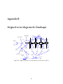
B Original sector diagrams for Zambaqui
81
C Boosd grammar deﬁnition
83
3
List of Figures
3.1
Bicycle inheritance hierarchy . . . . . . . . . . . . . . . . . . . . . . . . . . . . . . . .
19
3.2
Interface of an automobile . . . . . . . . . . . . . . . . . . . . . . . . . . . . . . . . .
23
3.3
Car interiors . . . . . . . . . . . . . . . . . . . . . . . . . . . . . . . . . . . . . . . .
24
(a)
Chevy Volt interior . . . . . . . . . . . . . . . . . . . . . . . . . . . . . . . . .
24
(b)
F350 pickup truck interior . . . . . . . . . . . . . . . . . . . . . . . . . . . . .
24
4.1
Manufacturing and retailing subsystem diagram . . . . . . . . . . . . . . . . . . . . . .
32
4.2
Policy structure diagram . . . . . . . . . . . . . . . . . . . . . . . . . . . . . . . . . .
34
5.1
Bathtub1 model deﬁnition . . . . . . . . . . . . . . . . . . . . . . . . . . . . . . . . .
39
5.2
Main model: Bathtub1 model usage . . . . . . . . . . . . . . . . . . . . . . . . . . . .
40
5.3
Bathtub2 model, with required parameters . . . . . . . . . . . . . . . . . . . . . . . .
41
5.4
Main model: Bathtub2 model usage . . . . . . . . . . . . . . . . . . . . . . . . . . . .
42
5.5
Smooth3I model implementation . . . . . . . . . . . . . . . . . . . . . . . . . . . . .
43
5.6
Bathtub With Inﬂow model, subclass of Bathtub2 . . . . . . . . . . . . . . . . . . . . .
44
5.7
Smooth3 model as a subclass of Smooth3I . . . . . . . . . . . . . . . . . . . . . . . . .
46
5.8
Shower temperature model with Smooth3 . . . . . . . . . . . . . . . . . . . . . . . . .
46
5.9
Water User interface . . . . . . . . . . . . . . . . . . . . . . . . . . . . . . . . . . . .
47
5.10 Policy-driven greenhouse model . . . . . . . . . . . . . . . . . . . . . . . . . . . . . .
48
5.11 A house, with an array of Water Users . . . . . . . . . . . . . . . . . . . . . . . . . . .
49
5.12 A piece of property containing a house . . . . . . . . . . . . . . . . . . . . . . . . . .
50
5.13 An interface to population models . . . . . . . . . . . . . . . . . . . . . . . . . . . . .
51
5.14 Advanced population model . . . . . . . . . . . . . . . . . . . . . . . . . . . . . . . .
52
4
5.15 Simple population model . . . . . . . . . . . . . . . . . . . . . . . . . . . . . . . . . .
52
6.1
Start of main Zambaqui model . . . . . . . . . . . . . . . . . . . . . . . . . . . . . . .
54
6.2
Creating a new model for the society sector . . . . . . . . . . . . . . . . . . . . . . . .
56
6.3
Empty ZamSociety model . . . . . . . . . . . . . . . . . . . . . . . . . . . . . . . . .
57
6.4
Main Zambaqui model with society fully deﬁned . . . . . . . . . . . . . . . . . . . . .
57
6.5
Creating and deﬁning the population submodel . . . . . . . . . . . . . . . . . . . . . .
58
(a)
Society model with population added . . . . . . . . . . . . . . . . . . . . . . .
58
(b)
Creating a new model for the population submodel . . . . . . . . . . . . . . . .
58
6.6
ZamPopulation model details . . . . . . . . . . . . . . . . . . . . . . . . . . . . . . .
59
6.7
Society sector with fully deﬁned population model . . . . . . . . . . . . . . . . . . . .
59
6.8
Births policy structure model details . . . . . . . . . . . . . . . . . . . . . . . . . . . .
60
6.9
Education model . . . . . . . . . . . . . . . . . . . . . . . . . . . . . . . . . . . . . .
61
6.10 Economy and population interfaces . . . . . . . . . . . . . . . . . . . . . . . . . . . .
62
6.11 Economy model for testing . . . . . . . . . . . . . . . . . . . . . . . . . . . . . . . . .
63
6.12 Society with population and education . . . . . . . . . . . . . . . . . . . . . . . . . .
63
6.13 Society with population and education connected . . . . . . . . . . . . . . . . . . . . .
64
6.14 Society with population, education and health sectors . . . . . . . . . . . . . . . . . . .
65
6.15 Society connected to the economy . . . . . . . . . . . . . . . . . . . . . . . . . . . . .
66
6.16 Completed Zambaqui main model . . . . . . . . . . . . . . . . . . . . . . . . . . . .
67
7.1
Society with a highlighted feedback loop . . . . . . . . . . . . . . . . . . . . . . . . .
71
A.1 Model deﬁnitions . . . . . . . . . . . . . . . . . . . . . . . . . . . . . . . . . . . . . .
78
A.2 Diagram symbols . . . . . . . . . . . . . . . . . . . . . . . . . . . . . . . . . . . . . .
78
A.3 Standard diagram connectors . . . . . . . . . . . . . . . . . . . . . . . . . . . . . . .
79
(a)
Information link . . . . . . . . . . . . . . . . . . . . . . . . . . . . . . . . . . .
79
(b)
Multi-link from model . . . . . . . . . . . . . . . . . . . . . . . . . . . . . . .
79
(c)
Flow . . . . . . . . . . . . . . . . . . . . . . . . . . . . . . . . . . . . . . . . .
79
A.4 Diagram color key . . . . . . . . . . . . . . . . . . . . . . . . . . . . . . . . . . . . .
80
(a)
Black - new structure . . . . . . . . . . . . . . . . . . . . . . . . . . . . . . . .
5
80
(b)
Gray - inherited structure . . . . . . . . . . . . . . . . . . . . . . . . . . . . . .
80
(c)
Blue - subclass-speciﬁc structure . . . . . . . . . . . . . . . . . . . . . . . . . . .
80
(d)
Red - required parameters . . . . . . . . . . . . . . . . . . . . . . . . . . . . . .
80
B.1
Original population sector formulation, from Pedercini [2011] . . . . . . . . . . . . . .
81
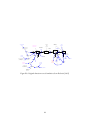
B.2
Original education sector formulation, from Pedercini [2011] . . . . . . . . . . . . . .
82
6
Listings
2.1
”Addition” . . . . . . . . . . . . . . . . . . . . . . . . . . . . . . . . . . . . . . . . .
12
2.2
”Car” . . . . . . . . . . . . . . . . . . . . . . . . . . . . . . . . . . . . . . . . . . . .
13
2.3
”Warehouse class example 1” . . . . . . . . . . . . . . . . . . . . . . . . . . . . . . . .
14
3.1
”Warehouse class example 2” . . . . . . . . . . . . . . . . . . . . . . . . . . . . . . . .
18
3.2
”Bicycles 1” . . . . . . . . . . . . . . . . . . . . . . . . . . . . . . . . . . . . . . . . .
20
3.3
”Bicycles 2” . . . . . . . . . . . . . . . . . . . . . . . . . . . . . . . . . . . . . . . . .
21
3.4
”Bicycles 3” . . . . . . . . . . . . . . . . . . . . . . . . . . . . . . . . . . . . . . . . .
22
3.5
”Interfaces 1” . . . . . . . . . . . . . . . . . . . . . . . . . . . . . . . . . . . . . . . .
26
3.6
”Teenager” . . . . . . . . . . . . . . . . . . . . . . . . . . . . . . . . . . . . . . . . .
27
3.7
”Interfaces 2” . . . . . . . . . . . . . . . . . . . . . . . . . . . . . . . . . . . . . . . .
28
4.1
DYNAMO DELAY1 macro [Richardson and Pugh, 1988] . . . . . . . . . . . . . . . .
31
C.1 Boosd grammar . . . . . . . . . . . . . . . . . . . . . . . . . . . . . . . . . . . . . . .
83
7
Chapter 1
Introduction
System dynamics is a methodology for improving the understanding and management of complex systems.
What sets it apart from other methodologies like systems thinking is the focus system dynamics has on
computer simulation, on quantifying and rigorously testing assumptions and understanding. is puts
the simulation model at the center of the system dynamics approach. ese models are simpliﬁed versions
of reality where we can test our assumptions and policies. At times, however, these simpliﬁed versions of
reality can become quite complex themselves.
Approaching dynamic problems that require a signiﬁcant level of detail, such as those that might be required when modeling a large business organization or national economy, puts a lower bounds on the
complexity of the model. A simple model may be easy to understand, but if it cannot match the reference mode it is not very helpful in understanding the dynamic problem at hand. Additionally, as Forrester
[1989] notes, complex models more closely match reality, and consequently are less subject to criticisms
of important pieces being le out.
In the beginning, system dynamics modeling was a multiple-medium exercise [Morecro, 1982]. e
modeling process started by sketching out stock and ﬂow diagrams of the problem. Once the structure
was decided upon, equations would be entered into a computer in the DYNAMO simulation language.
is was an iterative process until both the stock and ﬂow structure and equation structure matched the
8
reference modes of behavior, or otherwise addresses the dynamic problem. A later development to the
modeling process was adding causal loop diagrams to papers and reports to aid in the articulation of the
major feedback loops of a model. ese causal loop diagrams are oen the “distillation of understanding
which may have taken months or years to achieve” [Morecro, 1982].
In the mid-1980s, relatively inexpensive personal computers with graphical user interfaces were becoming
widely available. e Macintosh, followed by the IBM PC with Windows, were making computing accessible in a whole new way. is encouraged and enabled graphical modeling soware to be developed
which combined model layout/sketching with equation editing.
1.1
Managing Complexity
Subsystem diagrams and causal loop diagrams are two approaches for managing the complexity in presenting models to both other system dynamicists and clients. Some system dynamics tools like iink and
Powersim support hierarchical modeling, allowing you to nest models in much the same way subsystem
diagrams present structure.
Despite this, many prominent large models like C-ROADS and reshold 21 are still built ﬂatly using just
stock and ﬂow structures. Building sophisticated models in this manner is diﬃcult, and can cause diﬃculty communicating model results [Baker and Mullen, 2000]. In large models, there is a lot of complexity
inherent in the dynamics of the problem. Large ﬂat models introduce incidental complexity, complexity
that arise from the medium in which we are trying to solve the problem [Fogus, 2011]. In this case, creating a several thousand equation stock and ﬂow model imposes a lot of work on the modeler trying to
understand how pieces interact. Supplementary tools like causal tracing can help, but they don’t cancel
out the increase in complexity from having a ﬂat model.
Soware developers found themselves in a similar situation in the 80s and 90s. Programs were getting
larger and more complex. When once a text-based program would suﬃce, users were beginning to expect
feature-rich graphical applications. e standard programming languages of the time, such as C, made
9
easy a sprawling, hard-to-maintain style of program that was ill-suited to this new soware market.
A number of diﬀerent programming paradigms were available to help manage complexity, such as logical
and functional programming, but languages based on the object-oriented paradigm gained and have maintained dominance in the soware development community since the mid-1990s [TIOBE, 2011]. While it
has its roots at MIT in the 1950s, the object-orientated paradigm was formalized and popularized through
the development of the Simula language at the University of Oslo [Dahl and Nygaard, 1967]. In brief, the
“object” in object-oriented programming is the grouping of data together with methods, methods being
deﬁned as the relevant program structure (code) whose behavior depends on the associated data. Simula
was the main inﬂuence in the development of C++, which itself was the main inﬂuence on the development of Java; Java and C++ are the two most popular object-oriented programming languages. In 2011,
the majority of the programming languages used were object-oriented [TIOBE, 2011].
Object orientation has proven to be the most popular conceptual amework used to manage complexity in
soware development. is raises the question: can object-oriented concepts and techniques be applied to system
dynamics to help manage model complexity.
1.2
Overview
Chapter 2 deﬁnes deﬁnitions necessary for the introduction of object-orientation, such as those for types,
classes and objects. e next chapter, 3, introduces object-oriented concepts, such as polymorphism, encapsulation and inheritance, along with speciﬁc techniques – applications of object-oriented concepts in
speciﬁc programming languages. Chapter 4 reviews previous applications of object-oriented principles
and hierarchical modeling in system dynamics, such as DYNAMO macros and subsystem diagrams.
With a ﬁrm understanding of object-oriented approaches to managing complexity along with an introduction to prior work in system dynamics, chapter 5 describes this approach in applying object-orientation to
system dynamics. Chapter 6 walks through applying this approach to a large modeling project. Finally,
chapter 7 discusses the utility of this paradigm, some interesting options it opens up for modeling tools,
10
and discusses future directions of this research.
11
Chapter 2
Deﬁnitions
Before digging into the concepts of the object-oriented paradigm, it is necessary to deﬁne a number of basic
terms and concepts, such as what “objects” are. is chapter starts by exploring types and type systems.
Once types are deﬁned, classes of objects are introduced, followed by objects themselves.
2.1
Types
A type is classiﬁcation of a given piece of data. At the lowest level, all data on a computer is made up of ones
and zeroes; types give context to this binary data and deﬁne the operations that are allowed on any given
value or collection of values. When it comes down to it, types are what allow programs to turn commands
you give them, like “add these two things together”, into a set of instructions the computer understands.
Most languages have types to distinguish between things like sequences of text (character strings), integers
(whole numbers), booleans and ﬂoating-point (real) numbers. ese are known as primitive types, types
that represent the basic building blocks in a language. Consider the following example:
1
result = a + b
Listing 2.1: ”Addition”
12
For the computer to know what to do here, it must know the types of a and b. For example, if a and b
represent the strings “system ” and “dynamics”, the result might be the string “system dynamics”. However,
if a and b are integers, the result would be the addition of a and b. Similarly, if a and b are ﬂoating point
numbers, the result is still the addition of the two numbers, but the computer has to use a diﬀerent method
for the addition. Or, if the types of a and b aren’t compatible it could represent an error. For example, many
programming languages don’t allow adding text and a ﬂoating-point number, because that operation is
ambiguous – the intent could be to add the text-representation of the number to the string, but its equally
likely that it represents a logical error.
Usually, the programming system knows what the type of an object is by its declaration. In visual system
dynamics tools, when creating a variable the user also declares its type. is happens, for example, by drawing a stock symbol, or the ﬂow symbol, or telling the program that the auxiliary variable has an associated
lookup table. In most programming systems things are analogous, the ﬁst time you use a variable you have
to declare its name and type.
In addition to types like the primitives above, there are composite types. In many languages, composite
types are known as classes. As their name would suggest they are aggregations comprised of (usually)
named primitive and other composite types. An example would be a very coarse approximation of a car:
1 class Car {
2
int numberOfDoors;
3
Engine engine;
4
Wheel[] wheels;
5 }
Listing 2.2: ”Car”
is type deﬁnes how we represent cars. In this representation, we keep track of three pieces of data: a
simple integer counter of doors, a single composite object called the engine, and an array (noted by the
”[]”) of wheel objects. ese three pieces of data are named for what they represent: numberOfDoors,
engine, and wheels.
13
In short, types deﬁne the layout of and operations possible on a given piece of data. Historically, programming languages speciﬁed a ﬁx set of types. ese types (like integers, strings, booleans, and complex
structure types) were deﬁned in the language speciﬁcation, and your code could only use values that conformed to those types. Fortran didn’t support user-speciﬁed types until Fortran 90, which was released
over 30 years aer the initial version [Wikipedia, 2011]. e ability to specify new ﬁrst-class types, commonly called classes, is key to object-oriented programming.
2.2
Classes
A class is a user-deﬁned composite type like the Car example in listing 2.2 above. All classes are types, but
not all types are classes. It speciﬁes a collection of data along with a set of methods that are used to access
and manipulate the data. It is a group of attributes and behaviors. A method is a function (or subroutine, or
procedure) that is associated with a particular class. Imagine you wanted to create a simple representation
of a warehouse that holds widgets:
1 class Warehouse {
2
int inventory; // number of widgets on hand
3
4
// lets people view, but not modify, the current inventory level
5
public int getInventorySize() {
6
7
return inventory;
}
8
9
// add a number of widgets to our inventory, but make sure the
10
// number of widgets makes sense (is positive)
11
public void stock(int count) {
12
if (count > 0) {
13
inventory += number;
14
15
}
}
16
17
// fulfill a customers order, returns the number of widgets available
18
public int order(int count) {
14
19
// make sure we have a big enough inventory to fill the order
20
if (count > 0 \&\& count < inventory) {
21
inventory -= count;
22
} else if (count >= inventory) {
23
// if we don’t, give the customer all of our inventory
24
number = inventory;
25
inventory = 0;
26
} else {
27
// if we asked for an order of negative widgets, which
28
// doesn’t make sense, so don’t do anything
29
number = 0;
30
}
31
return number;
32
}
33 }
Listing 2.3: ”Warehouse class example 1”
In this example, the factory’s inventory can only be changed by calling the stock() method to add new
items, or by removing items when an order() comes in. e most complicated part is order fulﬁllment. It
is important to make sure that inventory never goes negative. Both stock() and order() also contain logic
to make sure that the factory handles negative order values correctly. All of this could be accomplished
by simply having an integer containing the inventory somewhere in your code program. In this case, the
beneﬁt of having a Factory class is that the code for checking extreme values and error conditions only has
be written once, in one place, and everywhere you use the factory beneﬁts.
2.3
Objects
In the real world, you encounter many individual objects (things) that are all of the same kind [Campione
et al., 2000]. Take a ﬂock of geese as an example. ese bird objects in the ﬂock are instances of the class
Bird (or perhaps of a more descriptive class like Geese). Because these individual goose instances share the
same class, you can interact with any bird in the same way, even though the details of individuals may vary.
You can command the bird to ﬂy(), perform a bird call(), perhaps even mate().
15
An object is a collection of state and methods to interact with that state. Each object is an instance of a
particular class, which describes the types of state and methods available.
e relationship between an object and its class is somewhat analogous to that of a simulation run and a
system dynamics model. e model deﬁnes the variables and equations of a system, but except for constants
and tables, doesn’t keep track of data. e model is strictly declarative. e simulation run is an instance
of a model, one of potentially many. Each run contains the actual values of variables of interest. Even if
runs started out with diﬀerent initial values or had diﬀerent decisions executed during the run, the set of
available variables doesn’t change, and you access the data in the same way.
16
Chapter 3
Object orientation
ere is a notable distinction between object-oriented concepts and object-oriented techniques [Myrtveit,
2000]. e main concepts of object oriented programming can be implemented in a number of diﬀerent
ways, making various techniques more or less useful. Two well-known object-oriented programming languages are Java and Ruby. ey both implement the concepts we’ll talk about below, but their diﬀerent
approaches lead to languages that feel and act signiﬁcantly diﬀerent [Ruby, 2011, Tate, 2006].
ere are 3 core object-oriented concepts: encapsulation, inheritance/delegation, and polymorphism (also
known as dynamic dispatch) [Scott, 2000].
3.1
Encapsulation
Encapsulation is the act of restricting access to some or all of the state of an object from other objects.
e canonical way this is done is by restricting access to the state of an object to the methods associated
with that class. e warehouse example in listing 2.3 clearly illustrates encapsulation. e only way to get
information about, or to change, the inventory of widgets is through the methods deﬁned by the class.
One of the major beneﬁts of encapsulation is that it hides the internal operations of your class behind a
17
consistent interface. is enables the programmer to restructure how the class works without having to
make changes throughout the projects source code in every place the class is currently being used. For
example, we could decide that our representation of a warehouse is too simplistic. In the real world, there
is a delay between receiving a new shipment of widgets and having them available for customers. One way
to restructure the class would be:
1 class Warehouse {
2
// inventory of widgets, with a 1 day delay between when items are
3
// received and when they’re available to fill orders
4
Queue inventory = new Queue(1, TimeUnit.DAY);
5
6
// lets people view, but not modify, the current level of
7
// available inventory
8
public int getInventorySize() {
9
return inventory.size();
10
}
11
12
// add a number of widgets to our inventory, but make sure the
13
// number of widgets makes sense (is positive)
14
public void stock(int count) {
15
16
inventory.add(count);
}
17
18
// fulfill a customers order, returns the number of widgets available
19
public int order(int count) {
20
21
return inventory.get(count);
}
22 }
Listing 3.1: ”Warehouse class example 2”
Here we’ve replaced the integer counter for inventory with an object that represents a time-delayed queue
of inventory. We’ve speciﬁed that this queue should always have a 1 day delay between when we add new
inventory and when its available to ﬁll orders. All 3 methods of our Warehouse class, getInventorySize(),
stock(), and order() now all simply call analogous methods on the inventory queue. is example is also
much shorter, because we assume that the ueue class now takes care of the error checking.
18
Places where the original Warehouse class are used won’t need to be changed to take advantage of the
more realistic behavior of this updated Warehouse, because they weren’t allowed to depend on the internal
implementation details of the original formulation. If the program had been allowed to directly access the
inventory counter, adding a delay would have been more work, with more places to make mistakes.
3.2
Inheritance and delegation
Inheritance and delegation are designed to enable the sharing of code and behavior. Having identical or
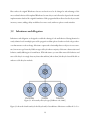
nearly-identical code in multiple parts of the program’s codebase places a burden on the developer whenever that structure needs to change. Inheritance captures the relationships between objects in a tree structure, known as a type hierarchy. Diﬀerent types of bicycles share a majority of the same characteristics and
behavior, usually diﬀering in a few small areas. With inheritance, you can deﬁne most of the behavior and
state of the bicycle in a single class, any classes that subclass (inherit from) this bicycle class will be able to
make use of the bicycles methods.
Figure 3.1: A hierarchy of bicycle types [Zakhour et al., 2006]
Figure 3.1 shows the class hierarchy for the Bicycle and 3 of its subclasses. Inheritance codiﬁes the “is-a” re-
19
lationships between classes of objects. A tandem bike is a kind of bicycle, same for both mountain and road
bikes. Subclasses can override, or redeﬁne, methods deﬁned in Bicycle that don’t ﬁt their needs, keeping the
rest. ey can also add additional methods. e tandem bike might add a method getNumberOfRiders(),
allowing you to ﬁnd out how many people are currently riding the tandem bicycle, which is not necessary
for the other types of bicycles. Similarly, the mountain bike will probably have to deﬁne its own behavior
for changing gears, as mountain bikes typically have more gears at a lower gear ratio than other bicycles.
1 class Bicycle {
2
public void changeGearTo(int newGear) {
3
4
// ...
}
5 }
6
7 class TandemBicycle extends Bicycle {
8
int riders;
9
public int getNumberOfRiders() {
10
11
return riders;
}
12 }
13
14 class MountainBicycle extends Bicycle {
15
public void changeGearTo(int newGear) {
16
17
// ...
}
18 }
Listing 3.2: ”Bicycles 1”
3.2.1 Delegation
Delegation is an alternate way of managing complexity by sharing code and behavior. While inheritance
captures is-a relationships, delegation promotes code use by enabling composition, known as has-a relationships. Going back to our bicycle diagram, with delegation, the particular types of bicycles, like MountainBicycles and RoadBicycles wouldn’t need to know the details of their particular gearing, they would
20
just delegate the responsibility for handling the message oﬀ to a separate object of type DriveChain. So
simply changing the type of the Bicycle’s DriveChain, as in listing 3.3 would cause the Bicycle to exhibit
diﬀerent behavior, without the need to change or override the Bicycles methods.
1 class Bicycle {
2
DriveChain driveChain = new StandardDriveChain();
3
public void changeGearTo(int newGear) {
4
5
driveChain.changeGearTo(newGear);
}
6 }
7
8 class MountainBicycle extends Bicycle {
9
DriveChain driveChain = new ExtraGearsDriveChain();
10
11
// no need to override changeGearTo, because all MountianBicycle’s
12
// driveChain objects Bicycle’s method will use the ExtraGearsDriveTrain
13 }
Listing 3.3: ”Bicycles 2”
Composition
Composition is one way of implementing delegation. Listing 3.3 was an example of composition in Java;
any time the changeGearsTo() method on a bicycle object was called, it would simply forward the method’s
argument to an identically named method on its driveTrain object, returning the driveTrain’s result to the
caller. is works well, but can get cumbersome for larger objects. Every time a method call needs to be
delegated to a particular component, a proxy method needs to created on the parent object, like the one
deﬁned in listing 3.3 on line 3 for Bicycle.
e Go language has an interesting technique to make composition easier called type embedding. Rather
than require proxy methods for every method a class intends to forward to a component, if a class does not
implement a given method but an embedded type does, the method is directly called on the embedded
type. In Go, we could rewrite listing 3.3, slightly reformulated, as follows:
21
1 type Drivechain interface {
2
ShiftUp()
3
ShiftDown()
4 }
5
6 type StandardDrivechain {}
7 func (*StandardDrivechain) ShiftUp() {
8
// check limits and shift to higher gear
9 }
10 func (*StandardDrivechain) ShiftDown() {
11
// check limits and shift to lower gear
12 }
13
14 type MountainDrivechain {}
15 func (*MountainDrivechain) ShiftUp() {
16
// check limits and shift to higher gear
17 }
18 func (*MountainDrivechain) ShiftDown() {
19
// check limits and shift to lower gear
20 }
21
22 type Bicycle {
23
Drivechain
24
Frame
25
Brakes
26
tires [2]Tire // an array of 2 tires
27 }
28
29 func NewRoadBicycle() *Bicycle {
30
return \&Bicycle{StandardDrivechain{}}
31 }
32
33 func NewMountainBicycle() *Bicycle {
34
return \&Bicycle{MountainDrivechain{}}
35 }
36
37 func main() {
38
bike1 := NewRoadBicycle()
39
bike2 := NewMountainBicycle()
22
40 }
Listing 3.4: ”Bicycles 3”
In the main function at the end of listing 3.4, two bicycles objects are created, one a mountain bike and
the other a road bike. When you call bike1.ShiUp(), bike1’s StandardDrivetrain instance’s ShiUp()
method is directly called. Composing objects like this takes some getting use to, but ends up being a very
productive programming style [Pike, 2010].
3.3
Polymorphism
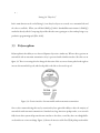
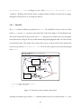
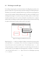
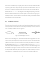
Polymorphism is the ability to use classes of disparate objects in a similar way. When a driver gets into an
automobile with an automatic transmission, they’re presented with a familiar interface, like that seen in
ﬁgure 3.2. ere is a steering wheel to change the direction of the car, an accelerator pedal on the right to
increase the automobile’s speed, and a break pedal on the le to decrease the speed.
steering
wheel
brake
gas
Figure 3.2: Generic interface of an automobile with an automatic transmission
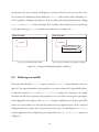
Once a driver masters driving their car, by extension they have gained the ability to drive the majority of
automobiles with automatic transmissions. Standard cars, large American pickup trucks, even cars with
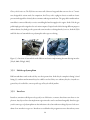
fully-electric drive systems all present the same interface to the driver, even if they have exceedingly diﬀerent form factors or inner workings. Figure 3.3 shows the interiors of the Ford F350 pickup truck and the
23
Chevy volt electric car. e F350 is a two-meter tall, 6.6-meter long truck that can tow close to 7 metric
tons, designed for serious work. In comparison, the Chevy volt is a plug-in electric car with an electric
powertrain designed for relatively short commutes and trips around town. e gas pedal in traditional automobiles is connected directly to a wire controlling fuel and air supply to the engine. In the Volt, the gas
pedal simply provides a signal to the car’s main computer. Despite both vehicles having diﬀerent purposes
and mechanics, they both give the operator the same interface to driving that they’re use to; both the F350
and Volt classes of automobiles are polymorphic with respect to driving.
(a) Chevy Volt interior
(b) F350 pickup truck interior
Figure 3.3: Interiors of automobiles with diﬀerent mechanics implementing the same driving interface
[Lloyd, 2008, Gillogly, 2009]
3.3.1 Subclass polymorphism
Diﬀerent subclasses can be used as if they were their parent class. In the bicycle examples in listing 3.2 and
listing 3.3, tandems and mountain bicycles could be used as if they were ordinary bicycles. Anywhere a
generic bicycle is called for, a more speciﬁc type of bicycle will do just ﬁne.
3.3.2 Interfaces
Interfaces, sometimes called protocols, specify a set of behavior, a contract, that classes can choose to implement. Any object whose class implements a given interface can be used interchangeably. Interfaces give
you the same type of polymorphism as class inheritance does, but without needing objects to be descendants of one another in a type tree. Interfaces are useful when the program cares more about how you use
24
objects, rather than how those objects are related to each other.
Interfaces are somewhat analogous to telephone jacks. e brand or details of the telephone are not important, as long as the cord for the telephone ﬁts in the wall jack and provides the telephone jack with
the right analog data. e phone could be a cordless phone, a wall-mounted phone, or even a computer
modem. All that matters to the telephone company’s system is that it the cord to the phone physically ﬁts
in the wall jack, and the data has the right form. It is not important to the telephone company if the signal
from a house is coming from the basement, or from a cordless phone in the yard. Similarly, a family can
go to the store and buy a replacement telephone without needing to call the telephone company and let
them know that the physical telephone is changing.
ere are times when the telephone doesn’t provide the correct interface. Several companies, such as Cisco,
now sell voice-over-IP (VOIP) telephones, which act more like computers than phones. e connector
used to hook them up to a phone system is physically diﬀerent – it is designed to be plugged into a data
network, not an analog telephone system. Old rotary telephones have the correct socket to connect them
to the telephone system, but the method they use to dial numbers (the pulse method) is no longer in use,
and may not work on some telephone systems even though they can physically be plugged into the system.
is is what interfaces provide for system dynamics. An interface allows you to specify the variables needed
(ﬁt of the jack), along with information about the type of data (ﬂows vs auxiliary data and units, for example).
Interfaces allow two models to interact without one needing to know the exact details of the other. A national model does not need to know the details of the population replacement telephone without needing
to call the telephone company and let them know that the physical telephone is changing.
ere are times when the telephone doesn’t provide the correct interface. Several companies, such as Cisco,
now sell voice-over-IP (VOIP) telephones, which act more like computers than phones. e connector
used to hook them up to a phone system is physically diﬀerent – it is designed to be plugged into a data
network, not an analog telephone system. Old rotary telephones have the correct socket to connect them
25
to the telephone system, but the method they use to dial numbers (the pulse method) is no longer in use,
and may not work on some telephone systems even though they can physically be plugged into the system.
is is what interfaces provide for system dynamics. An interface allows you to specify the variables needed
(ﬁt of the jack), along with information about the type of data (ﬂows vs auxiliary data and units, for example).
Interfaces allow two models to interact without one needing to know the exact details of the other. A
national model does not need to know the details of the population submodel, it only needs access to
indicators such as total population and labor size while providing the submodel with access to variables
such as average life expectancy and fertility rate needed to close the loop. Clearly deﬁning the interface to
the population submodel makes it much less complicated to change the structure of the population model
later, even if that means substituting a completely diﬀerent population model formulation.
1 class Bicycle implements Vehicle {
2
public void turn(float radians) {
3
// twist handlebars
4
}
5
public void accelerate(float rate) {
6
// downshift, stand up on pedals if rate is positive
7
}
8
public float getSpeed() {
9
10
// return information about our current speed
}
11 }
12
13 class Skateboard implements Vehicle {
14
public void turn(float radians) {
15
// lean left or right
16
}
17
public void accelerate(float rate) {
18
// kick with your feet more if rate is positive
19
}
20
public float getSpeed() {
21
22
// return information about our current speed
}
26
23 }
24
25 interface Vehicle {
26
public void turn(float radians);
27
public void accelerate(float rate);
28
public float getSpeed();
29 }
Listing 3.5: ”Interfaces 1”
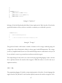
In listing 3.5, both the Skateboard and the Bicycle classes implement the Vehicle interface. If you had an
agent based simulation of how youth move around in a community, you could model a person as:
1 class Teenager {
2
Vehicle modeOfTransportation;
3
4
// rest of the details that define teenagers go here.
5 }
Listing 3.6: ”Teenager”
e agent based model could construct a number of instances of the teenager, randomly giving each
teenager object either a Skateboard or a Bicycle as that teenager’s modeOf Transportation. e teenager
(in this very simpliﬁed model) doesn’t care if his modeOf Transportation is a skateboard or a bicycle, all
he cares is that he can use it to get around town and interact with other agents.
e example listings 3.5 and 3.6 above were written in the Java programming language. In Java, each class
has to explicitly enumerate the interfaces that it supports. While this works, it is not the only way to
implement interfaces.
3.3.3 Go
e programming language Go includes a unique implementation of interfaces. In most languages that
support interfaces, like Java and C#, each class must explicitly enumerate the interfaces it supports. In Go,
27
any type which supports the set of methods listed in an interface automatically implements the interface.
In Go, our Vehicle example from listings 3.5 and 3.6 would look like:
1 type Bicycle struct{}
2 func (*Bicycle) Turn(radians float32) {
3
// twist handlebars
4 }
5 func (*Bicycle) Accelerate(rate float32) {
6
// downshift, stand up on pedals if rate is positive
7 }
8
9 func (*Bicycle) GetSpeed() float32 {
10
// return information about our current speed
11 }
12
13 type Skateboard struct{}
14 func (*Skateboard) Turn(radians float32) {
15
// lean left or right
16 }
17 func (*Skateboard) Accelerate(rate float32) {
18
// kick with your feet more if rate is positive
19 }
20 func (*Skateboard) GetSpeed() float32 {
21
// return information about our current speed
22 }
23
24 type Vehicle interface {
25
Turn(radians float32)
26
Accelerate(rate float32)
27
GetSpeed() float32
28 }
29
30 type Teenager struct {
31
modeOfTransportation Vehicle
32
// rest of the details that define teenagers go here.
33 }
Listing 3.7: ”Interfaces 2”
28
e advantage of Go’s approach is that you can create and use new interfaces without having to modify any
existing types to work with them. If you have existing types that have already implemented the methods
you list in your interface, you can immediately use them without modiﬁcation where ever that interface is
called for.
29
Chapter 4
Previous approaches in SD
ere is a long history of attempts to encourage encapsulation and hierarchy into the system dynamics
modeling process, as well as several experiments and implementations that are explicitly object-oriented.
DYNAMO, the ﬁrst system dynamics modeling language1 , had built-in functions that could be used to
generate common model structures, like smooth and delay3 [Richardson and Pugh, 1988]. In addition to
common built in functions, it allowed modelers to deﬁne their own macros, which were called like regular
functions, but computed their values based on DYNAMO statements. In the 1970s, subsystem and policy
diagrams were introduced to help manage complexity when applying the production sector of the National
Economic Model to speciﬁc business applications and to aid in teaching the Industrial Dynamics model
[Morecro, 1982].
Recently, Magne Myrtviet has published much research about how to apply object-oriented programming
to system dynamics, including information hiding and polymorphism. Jim Hines has published work on
a model construction approach based around successive rounds of replacing more general model structure
with more speciﬁc structure. Finally, several system dynamics modeling tools have various levels of support
for hierarchical and modular modeling.
1
ere was a program called SIMPLE which predated DYNAMO, but it was not considered complete and did not see
widespread use [Haigh, 2005].
30
4.0.4 DYNAMO Macros
Modelers equently discover that they must repeat a pattern of statements or expressions a number of diﬀerent places in a model. e ability to devise a shorthand notation for such repeated
structures would save the modeler time while constructing the model. Model readers would also
beneﬁt by quickly being able to master the structure once and quickly recognize it wherever it is
used. – Richardson and Pugh [1988]
e DYNAMO language included built-in support for macros. Macros deﬁne a mathematical operation
or a commonly used set of model structure. Once deﬁned, the macro can be used elsewhere in the model.
Deﬁning macros is analogous to deﬁning a class in an object-oriented programming language. You can
deﬁne an arbitrary number of stocks and auxiliary variables in the macro to use as intermediate variables
in the formulation of the return value. Every time the macro is used (which is analogous to class instantiation) private, hidden copies of those variables are created and added to the model structure. Each use
of the macro gets its own copies of the variables. Listing 4.1 shows the implementation of DELAY1 in
DYNAMO2 .
1 MACRO DELAY1(IN,DELAY)
2 A DELAY1=$LV/DELAY
3 L $LV.K=$LV.J+DT*(IN.JK-DELAY1.J)
4 N $LV=DELAY*IN
5 MEND
Listing 4.1: DYNAMO DELAY1 macro [Richardson and Pugh, 1988]
In macro deﬁnitions, variables whose name started with a dollar sign were private to instances of that
macro, such as $LV in listing 4.1. e value of the macro was determined by the equation of a variable with
the macro name, DELAY1 in this case.
Along with this macro support came a number of built-in functions to encapsulate common model structure. As we saw in listing 4.1, these functions (like the DELAYs and SMOOTH) were implemented as
2
In DYNAMO, spaces are not allowed in variable deﬁnitions, making the formulations harder to read than necessary.
31
macros [Richardson and Pugh, 1988]. Rather than having to create 3 stocks and deﬁne their inﬂows and
outﬂows every time a 3rd order exponential delay is needed, the DELAY3 function was available be used to
the same eﬀect. is decreased model complexity by reducing the number of equations in the model (along
with the chance for typos), and explicitly naming interesting structures, like SMOOTH and RAMP.
4.0.5 Subsystem and policy diagrams
In the early years of system dynamics, the only diagrams used to convey the structure of models were stock
and ﬂow diagrams [Morecro, 1982]. Forrester’s Industrial Dynamics doesn’t include any visual overview
of model structure, it simply has a collection of individual stock and ﬂow diagrams representing diﬀerent
pieces of the model. Using causal loop diagrams (CLDs) to convey the dominant feedback loops in a
model ﬁrst appears in Forrester [1968]. Morecro notes that the causal loop diagram represents not the
conceptual origin of the model, but a reﬁned product of the modeling process [Morecro, 1982]; CLDs
are used to give a less complex, less detailed overview of parts of the model considered important.
To overcome certain weaknesses of causal loop diagrams and provide a high level view of the model that can
be used during model construction, subsystem and policy diagrams were introduced [Morecro, 1982].
Subsystem diagrams show major subsystems, such as organizational divisions in a social or industrial system.
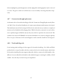
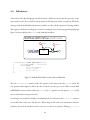
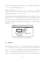
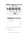
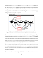
Figure 4.2 is a subsystem model of a manufacturing and retailing system. It shows the three main subsystems of the model, retail, production and shipping control, and labor procurement, along with the feedback loops and material ﬂows between them. e details of these three subsystems would all be deﬁned in
separate subsystem or policy structure diagrams.
Subsystem diagrams like ﬁgure 4.2 provide a similar view of the major feedback loops of a model, but have
the advantage that they can be used throughout the modeling process, and are especially valuable at the
start. As Morecro notes, “policy diagram stands in a natural hierarchical relationship above [equation]
formulation”.
32
Figure 4.1: A subsystem diagram representing manufacturing and retailing, ﬁgure 3 from Morecro
[1982]
is view of subsystems ﬁts cleanly into an object-oriented paradigm. e behavior of diﬀerent parts of
the model is cleanly delegated to more specialized sub-models.
Subsystem and policy structure diagrams were used in introductory courses at MIT Sloan with the Industrial Dynamics model [Morecro, 1979]. Corporate systems were broken down into component functional areas, such as production control, labor procurement, pricing and marketing. Students commented
favorably on the approach.
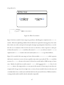
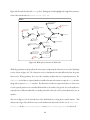
Figure 4.2 shows a policy structure diagram of a marketing system. In it, values from other subsystems are
used, along with values endogenous to the marketing subsystem, as inputs to policies. e value of these
policies are used both in the formulation of other policies, although they could also be used directly to control the rates of ﬂows. Policy structure diagrams put the focus on the decision-making process by ‘hiding’
the details of the decisions inside policies, which would be represented in another diagram. Interestingly
they also show diﬀerent levels of abstraction in the same diagram; ﬁgure 4.2 has policies and subsystems,
which themselves potentially contain additional policies or subsystems, alongside traditional stocks and
ﬂows.
33
Figure 4.2: A policy structure diagram of a market subsystem, ﬁgure 6 from Morecro [1982]
4.0.6 Object-oriented extensions to system dynamics
Magne Myrtveit has written extensively about how to extend system dynamics with object oriented concepts. Object Oriented Extensions to System Dynamics [Myrtveit, 2000] lays out one possible way to
approach system dynamics modeling with an object-oriented paradigm.
Components are deﬁned as a pieces of model structure which may be used as the building-blocks of other
components. Components may specify interfaces which deﬁne the pieces of their structure that are available to other parts of the model. Any two components which identical interfaces may be interchanged,
allowing for polymorphism.
A key beneﬁt of this component-based object-oriented approach is that it would allow collections of
domain-speciﬁc building blocks to be assembled. ese collections would enable faster, more modular
model development. ey would also enable a division of labor between the component-modeler and the
integration-modeler.
Sockets and plugs are introduced as a way to simplify wiring together components into a cohesive model.
34
Sockets and plugs have particular signatures, and only a plug with a matching signature may be connected
to a socket. e goal is to allow non-technical users to create models by connecting ready-made components.
4.0.7 Construction through replacement
An alternative take on hierarchical modeling is oﬀered in Construction rough Replacement by Hines
et al. [2011]. In it, a hierarchical classiﬁcation of common system dynamics model structure is developed.
is classiﬁcation starts oﬀ with an unspeciﬁc SD molecule, and works its way toward more complicated
structures such as bathtub models and aging chains. With the hierarchy constructed, it is used to allow
users to quickly navigate and ﬁnd the structure they want, which is copied into the current model. is
is similar to how macros in DYNAMO create structure behind the scenes, only here it happens explicitly.
Once a new piece of structure is in the current diagram, it can be renamed to match how it is being used.
4.0.8 Visual modeling tools
Several existing visual modeling tools have support for hierarchical modeling. iSee’s Stella and iink
products has the concept of modules, which are containers for lower level model structure and the basis
for hierarchical modeling. Powersim supports submodels, which are containers for child variables. A key
diﬀerence between submodels and modules is that submodels support restricting the visibility of child
variables – this is the object-oriented concept of encapsulation.
35
Chapter 5
Methods
ere are a variety of object-oriented programming techniques and concepts that could be applied to system dynamics. e approach described here aims to minimize the incidental complexity that arises when
modeling moderate to large systems while providing a familiar visual system dynamics environment. e
new symbols and visual syntax presented here is summarized in appendix A.
In 2011, almost all system dynamics models are created in visual modeling programs1 . is paper introduces both extensions to the traditional system dynamics diagrams to enable object-oriented techniques,
along with a clean, concise textual representation of the object oriented models.
In large models, its oen necessary to look at the equation view of the model for veriﬁcation or debugging;
having an easy to navigate text-based format for this is an asset. It is similarly beneﬁcial when publishing
model results to have a clear and concise textual representation of model structure. is textual language
is called Boosd2 .
1
2
With the exception of some models on the Forio online simulation platforms
Boosd (written with a single initial capital) was initially an acronym for Bergen Object-Oriented System Dynamics
36
5.1
Vocabulary
In this approach, the basic unit of aggregation is known as a model. Stocks, ﬂows, auxiliary variables and
tables are what is known as primitive types, they are the atoms which are combined to form molecules
(models). Primitive types cannot contain any child variables, like a model can. A variable is a symbolic
name, a placeholder, for either the result of an equation or a model instance.
Models are alternatively called submodels, sectors, model classes, classes, and policy structure diagrams
when these alternative titles are less ambiguous. ey all refer to the same singular concept (although
policy structures may have a distinct visual representation).
5.1.1 Instances vs. Models
e distinction between an instance of a model and the model’s deﬁnition, as described in chapter 2 is very
important. It is not new, as the concept applies to Dynamo macros and built-in function as well, but being
comfortable with the concept is key to this object oriented approach.
5.2
Projects
A system dynamics modeling project typically results in the creation of a model, reports on the structure
and behavior of the model, and potentially a management ﬂight simulator. With an object oriented approach, the creation of that ﬁnal simulation model may result in the creation of numerous ‘sub’-models.
Accordingly, the approach described here structures things in terms of ‘modeling projects’ rather than
‘models’.
A modeling project can be classiﬁed as either a ’library’ or ’simulation’ project. A simulation project deﬁnes
a model named ‘main’ along with any supplementary models developed in the course of the project. For
example, the model of a ﬁrm may have submodels for retail, production and labor. e main model would
contain an instance of each of these models with the necessary feedback loops connected between them.
37
If the modeler followed the conventions in ?, the production model would be a policy structure diagram
composed of several stocks, along with models representing each major policy decision involved in the
production process.
A library project contains the deﬁnitions of a number of models, but doesn’t contain a main model. A
library is useful for a modeler, modeling team, or larger organization as a way to aggregate and distribute
models representing their collective modeling experience and wisdom. Model libraries can easily be imported into new projects, saving the modeler from having to re-implement common structure in every new
modeling project. e standard structures provided by a modeling tool can be thought of as belonging to
a single library project.
5.3
Models
Model deﬁnitions are how all models and submodels are speciﬁed. Where it is more readable, this paper
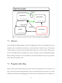
will use the object-oriented terminology, where models are referred to as classes, and instances of models
as objects.
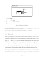
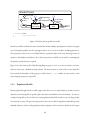
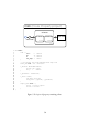
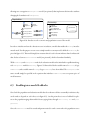
Figure 5.1 shows the deﬁnition of a bathtub model with no inﬂow and a single outﬂow. In Boosd, type
names come aer the variable names. is is primarily done to improve readability; when skimming
through a large model it is easier to read ‘bathtub stock’ than ‘stock bathtub’. If a variable doesn’t declare a type directly aer the name, before the equals sign, it is assumed by the compiler to be an auxiliary
variable. In other words, the deﬁnition of “delay” in ﬁgure 5.1 is equivalent to ‘delay
aux = 2 ‘minutes‘’.
e delay declaration also introduces the syntax for units. Units come aer an expression or a variable
declaration. Because units themselves may be expressions, such as ‘Rabbits/m²‘, it is necessary to have a
way to clearly delineate where equations end and units start. In Boosd backticks are used to mark the start
and end of unit equations.
Deﬁning a stock is done by specifying equations for a number of named initialization parameters. In the
bathtub example, we use two of them, outflow and initial.
38
outflow, biflow,
and inflow parameters are
Bathtub1
delay
tub
to drain
1 Bathtub1 model {
2
delay = 2 ‘minutes‘
3
to_drain flow = bathtub / delay
4
bathtub stock = {
5
outflow: to_drain
6
initial: 500 ‘liters‘
7
}
8 }
Figure 5.1: Bathtub1 model deﬁnition
optional, and a stock initialization may contain multiple outflows, inflows and biflows. e initial parameter is required, and each stock initialization must contain an initial expression.
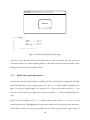
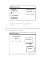
5.3.1 Main model
Because each modeling project (group of ﬁles) can deﬁne a number of models, it is necessary to have a
mechanism to decide which model to run when simulating the project. By convention, this is the model
named main. To run our Bathtub1 model, we would deﬁne a main model with a single instance of the
Bathtub object, along with speciﬁcations of how long the model should run for, as in ﬁgure 5.2. e
creation of an instance of the bathtub model is the same as initializing a stock, with the diﬀerence that the
Bathtub1
class name appears directly before the opening curly brace (‘{’) and the initialization parameters
are diﬀerent. In the case of this model of a bathtub, there aren’t any initialization parameters needed.
Time is a special variable in Boosd. It can only be deﬁned in the main model, to avoid confusion about
when the simulation should start, end and at which time step (dt) the model should run. It is initialized
39
main (Bathtub project)
bathtub
Bathtub1
1 main model {
2
time = {
3
start:
0
4
end:
60
5
dt:
.5
6
save_step: 1
7
}
8
9
bathtub = Bathtub1{}
10 }
‘minutes‘
‘minutes‘
‘minutes‘
‘minute‘
Figure 5.2: Main model: Bathtub1 model usage
as if it were a stock, but with the four named parameters start, end, dt, and save_step. Save step is used
in a similar manner to the Vensim modeling soware; it allows the model to be run with a small dt, while
limiting the amount of data recorded for analysis.
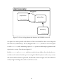
5.3.2 Model with required parameters
Its oen both convenient and useful for re-usability to be able to specify parts of a submodel, like delay
times and initial values, when creating an instance of it. e Bathtub1 model could be reformulated as in
ﬁgure 5.3, with three things changed. e equation for delay has been removed, the unit for delay has
been moved to directly aer the variable name, and a new variable initial has been added with liters for
units.
Figure 5.3 shows the addition of the initial variable, and the outlines of both initial and delay’s circle
symbols has turned red. is highlights the fact that these variables need to be speciﬁed when an instance
of the model is created. In a model, any variables that do not have equations must be given a value at
40
initialization time, similar to how the initial value must be speciﬁed for a stock. In the Bathtub2 model,
delay
and initial must be speciﬁed (initialized) when creating a new instance. e revised main model
which fully initializes Bathtub2 is shown in ﬁgure 5.4.
Bathtub2
initial
delay
tub
to drain
1 Bathtub2 model {
2
delay ‘minutes‘
3
initial ‘liters‘
4
to_drain flow = bathtub / delay
5
6
bathtub stock = {
7
outflow: to_drain
8
initial: initial
9
}
10 }
Figure 5.3: Bathtub2 model, with required parameters
5.3.3 Dynamo macro-like models
By making the creation and use of models a ﬁrst-class feature of the language, it makes it trivial to implement the built-in Dynamo macro functions like SMOOTH3I and DELAY1. e Boosd language uses
the same convention as Dynamo [Richardson and Pugh, 1988]: by giving a variable in a model the same
name as the model itself, referencing an instance of the model gives you the value of that variable for that
instance.
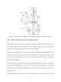
e Smooth3i and Smooth3 models are good illustrations of this. Figure 5.5 shows a typical implementation
of Smooth3I3 : there are 3 stocks and 3 biﬂows representing the goal/gap nature of the exponential smooth.
3
is is the formulation used in both the Stella and Vensim reference manuals.
41
main (Bathtub project)
bathtub
Bathtub2
1 main model {
2
time = {
3
start:
0 ‘minutes‘
4
end:
60 ‘minutes‘
5
dt:
.5 ‘minutes‘
6
save_step: 1 ‘minute‘
7
}
8
9
bathtub = Bathtub2{
10
initial: 500 ‘liters‘
11
delay:
2
‘minutes‘
12
}
13 }
Figure 5.4: Main model: Bathtub2 model usage
42
e three required parameters for Smooth3i are initial, input, and delay.
Smooth3i
input
initial
level 1
change in 1
level 2
change in 2
delay
smooth3i
change in 3
1 Smooth3I model {
2
input
3
initial
4
delay ‘time‘
5
6
change_in_1 = (input - level1)/delay
7
change_in_2 = (level1 - level2)/delay
8
change_in_3 = (level2 - smooth3)/delay
9
10
level1 stock = {
11
biflow: change_in_1
12
initial: initial
13
}
14
15
level2 stock = {
16
biflow: change_in_2
17
initial: initial
18
}
19
20
smooth3i stock = {
21
biflow: change_in_3
22
initial: initial
23
}
24 }
Figure 5.5: Smooth3I model implementation
e ﬁnal stock in the cascade is named smooth3i, the same name as the model. is allows users to assign
an instance of the Smooth3I model to a variable, and simply reference that variable’s name to get the value
of the smooth3i stock, as you would with the SMOOTH3I Dynamo macro or any of the smooth built in
functions in the existing graphical tools.
43
5.4
Inheritance
A key feature of the Boosd language is model inheritance. Models can declare that they specialize, or subclass, another model. e model that a class specializes is called its parent model, or superclass. When subclassing, a model may add additional structure (variables), as well as redeﬁne equations of existing variables.
is equation redeﬁnition is analogous to method overriding in object-oriented programming languages.
Figure 5.6 shows subclasses the Bathtub2 model and adds an inﬂow.
Bathtub With Inflow (Bathtub2)
initial
delay
tub
from plumbing
to drain
1 BathtubWithInflow model specializes Bathtub2 {
2
from_plumbing flow = 2 ‘liters/minute‘
3
bathtub stock = {
4
inflow: from_plumbing
5
outflow: to_drain
6
initial: initial
7
}
8 }
Figure 5.6: Bathtub With Inﬂow model, subclass of Bathtub2
e new BathtubWithInflow model overrides the equation for the main stock of the Bathtub2 model. e
new equation adds a single new inﬂow, the value of which is two liters per second. When created, BathtubWithInﬂow instances still need the same initial and delay parameters of the parent Bathtub2 model;
they are inherited from the parent model.
Something to note is that Boosd makes a clear distinction between functions, like if_then_else, and common models that contain state, like Smooth. When using models, such as for information and material delays, they must be initialized on their own, not as a value in an equation. Writing, nput:a_stock;
44
delay:3apparent = 2 * Smoothi
would give an error, while
nput:2*a_stock;
delay:3apparent = Smoothi
would not. ‘Hiding’ model structure inside of equations limits the ability of visual tools to navigate
through the model structure, so it is simply not allowed.
5.4.1 Smooth3
e Smooth3 model is a subclass, a specialization of Smooth3i. e only diﬀerence between the two models
is that Smooth3 uses the input parameter as the initial value of the stocks. Figure 5.7 clearly illustrates this.
e structure inherited from the parent model Smooth3i has grayed out variable names, representing the
fact that they haven’t changed. e only variable that has changed is highlighted in blue; the value of initial
is now based on input. is change is also evident in the text-view of the model: the only equation that
needs to be speciﬁed for Smooth3 is initial
= input,
all of the other equations are inherited unchanged
from Smooth3i.
Smooth3 (Smooth3I)
input
initial
level 1
change in 1
level 2
change in 2
delay
smooth3i
change in 3
1 Smooth3 model specializes Smooth3I {
2
initial = input
3 }
Figure 5.7: Smooth3 model as a subclass of Smooth3I
A perhaps non-intuitive aspect of this Smooth3 subclass is that because no new variable named smooth3 (the
45
name of the model) was added, a reference to an instance of Smooth3 in an equation will yield the value of
the Smooth3i stock, as it does for the parent model Smooth3i
In ﬁgure 5.8, the equation for perceived
temp
is Smooth3{input:
shower_temperature; delay: 10}.
is is
similar to how you would use the smooth3 function in Vensim, or smth3 in iSee soware, with the diﬀerence that in Boosd parameters like input and delay are named.
Figure 5.8 shows a simple goal/gap policy regulating the temperature of a shower. By having Smooth3 implemented as a model, perceived
temp is clearly identiﬁed in the shower temperature model as an information
delay, without the need for examining the equation or adhering to a particular naming convention for variables. Additionally, graphical soware could enable users to ‘zoom-into’ the Smooth3, ﬁgure 5.7, model by
clicking on perceived
temp.
main (Shower Temperature proj.)
delay
shower
temperature
temp change
perceived
temp
temp goal
Smooth3
Figure 5.8: Shower temperature model with Smooth3
5.5
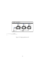
Interfaces
Figure 5.9 deﬁnes an interface named Water
Water User
User.
e visual representation may look out of place at ﬁrst;
is designed to present a consistent view (interface) of any model that has volumetric ﬂows
named from
plumbing
and to
drain,
whether that is a model of a shower, bathtub, sink, washing machine,
greenhouse, or even a pool. In ﬁgure 5.9’s diagram, it does not show what is in between the from
and the to
plumbing
drain ﬂows; in fact that is the point of an interface, to allow the use of a model without knowing
46
the speciﬁcs of it.
Water User
from plumbing
to drain
1 WaterUser interface {
2
from_plumbing flow ‘liters/minute‘
3
to_drain
flow ‘liters/minute‘
4 }
Figure 5.9: Water User interface
Figure 5.10 shows a model of water usage in a greenhouse, which happens to implement the Water
User
interface. Water from plumbing is added to ﬂower beds based on a particular watering policy. Once in the
ﬂower beds, water either ends up in the atmosphere through evapotranspiration from ﬂowers, or on the
ﬂoor due to over-saturation of the soil. Once the water is on the ﬂoor, it either evaporates or ends up in
the drain. Because the Greenhouse model has a ﬂow named from
implements the Water
plumbing as well as one named to drain, it
User interface and can be used anywhere a Water User is speciﬁed/called for.
Figure 5.11 is a model of the water usage in a house. It has an inﬂow from
water source
which represents
that house’s connection to a source of water, typically a water main or personal well. e House model has
an array of Water
Userss,
because each instance of a house has a varied number of diﬀerent types of water
users. Finally, the model has an outﬂow named to
Water User
septic,
which aggregates the to
drain
ﬂow of each
instance. By using interfaces, we can represent the structure of water usage in most houses in
a single model: they get water from a single source, a variety of users around the house use that water and
eventually drain it into a central system, and that drain leaves the system of the house. Without interfaces,
creating a similar model would be either be awkward or impossible.
47
Greenhouse
time of day
temperature
watering
policy
evaporation
from floor
evapotranspiration
water in
flower beds
from plumbing
water on
floor
to floor
to drain
1 Greenhouse model {
2
// <equations omitted>
3 }
Figure 5.10: Policy-driven greenhouse model
Interfaces would be useful for the class of models that include multiple participants in a market. A typical
way of solving this problem involves arraying an entire sector, or view, of variables, including parameters.
Some parameters may be set to 0 to disable them for a particular index of the array. By using an array of
interfaces, what had previously been a ‘slice’ of the arrayed sector could be its own model, containing only
the parameters and structures required.
Figure 5.12 is the main model of this Housing Property project. In it, we create an instance of a house
with two water users: a bathtub and a greenhouse. e house instance is connected to a water main ﬂow
from outside the boundaries of the property, and the house’s to
septic
outﬂow is connected to a stock
representing the property’s septic ﬁeld.
5.5.1 Population Models
Polymorphism through interfaces enables approaches that were not easily feasible previously in system
dynamics, such as being able to quickly replace alternative formulations of model structure. A concrete
example is being able to choose which of several population submodels is used in a run of a larger model
of a national economy. e general requirements in this case are that the population submodels provide
standard indicators, such as total population and net migration, and can reference data from other parts
48
House
water users
bathtub
bathtub
from water
source
Bathtub1
Bathtub1
[]WaterUser
to septic
1 House model {
2
from_water_source ‘liters/min‘
3
to_septic ‘liters/min‘
4
5
water_users []WaterUser = {
6
from_plumbing: from_main
7
to_drain: to_septic
8
}
9 }
Figure 5.11: A house, with an array of Water Users
of the model, such as average life expectancy, to close the feedback loops.
For a detailed analysis intended for peers with modeling experience, a population model based on an aging
chain of yearly cohorts, broken up by sex, might be most appropriate. For policymakers who are more interested in the national model’s insights into tax formulation and government regulation, removing complexity in other parts of the model could be desirable. In this case, a simple three-stock aging chain population
sector would be suﬃcient.
In this example, inheritance is not an eﬀective strategy. e two diﬀerent population submodels do not
share any signiﬁcant structure; one centers on an array-based aging chain, the other on an explicit threestock one. Inheritance is appropriate when there is structure in one model that is extended or changed in
another, not simply when two ideas are conceptually similar.
49
main (House Property project)
a house
a shower
a bathtub
septic field
water main
Shower
Bathtub1
House
1 main model {
2
time = {
3
start:
0 ‘minutes‘
4
end:
60 ‘minutes‘
5
dt:
.5 ‘minutes‘
6
save_step: 1 ‘minute‘
7
}
8
9
// this defines the house’s maximum water usage rate
10
water_main flow = 100 ‘liters/min‘
11
12
a_bathtub = BathtubWithInflow{
13
initial: 500 ‘liters‘
14
delay:
2
‘minutes‘
15
}
16
17
a_greenhouse = Greenhouse{}
18
19
a_house = House{
20
from_main: water_main
21
water_users: (a_bathtub, a_greenhouse)
22
}
23
24
septic_field stock = {
25
inflow: a_house.to_septic
26
initial: 0 ‘liters‘
27
}
28 }
Figure 5.12: A piece of property containing a house
50
Population
total
population
births
deaths
youth population
labor force
1 Population interface {
2
births flow ‘Individuals/time‘
3
deaths flow ‘Individuals/time‘
4
5
total_population ‘Individuals‘
6
youth_population ‘Individuals‘
7
labor_force
‘Individuals‘
8 }
Figure 5.13: An interface to population models
Advanced Population
per capita
income
births
access to
clean water
migration
total
population
per capita
GDP
deaths
[Ages]
access to
healthcare
adult literacy rate
youth population
labor force
1 AdvancedPopulation model {
2
// <details omitted>
3 }
Figure 5.14: An advanced formulation of a population model with policy symbols, indicating this population model has 3 sub-models: births, deaths and migrations.
51
Simple Population
youth
deaths
labor
force
youth
births
elderly
deaths
adult
deaths
elderly
adult
to elderly
youth
to adult
total population
birth rate
1 SimplePopulation model {
2
// <details omitted>
3 }
Figure 5.15: Simple population model
52
Chapter 6
e object-oriented modeling process
Modeling with an object-oriented approach takes a much more top-down approach than is usually found
in system dynamics. is chapter works through the application of the object-oriented modeling paradigm
to a moderately-sized system dynamics project. Because system dynamics takes a strongly visual approach
to specifying model structure, this chapter occasionally refers to actions the user of a hypothetical modeling
program would take in that (hypothetical) program. is is necessary to give the reader a sense of the actual
object-oriented process, as opposed to simply staying at the conceptual level.
e example used is a version of the Millennium Institute’s reshold 21 (T21) Minimum Country Model
(MCM), a simpliﬁed version of the full T21 model [Kopainsky et al., 2010, Pedercini et al., 2007, Pedercini, 2007]. Here, the MCM will be built and parameterized for a ﬁctional but prototypical West African
nation named Zambaqui. Zambaqui was created for use in the GEO-SD 321 course, “Model-based Socioeconomic Planning”, at the University of Bergen. It is introduced as a prototypical West African nation
facing a number of challenges in three sectors: society, economy and the environment. ese challenges
are shown in table 6.1. Given this problem formulation, it is natural to start the model with a similar
structure.
Figure 6.1 shows a new main model for the Zambaqui project with three submodels: society, economy, and
environment.
So far, the system dynamics model corresponds directly to the conceptual structure of the
53
Challenge
Society
Low Life Expectancy
Low Literacy Rate
Low Access to Health Care
Poor Infrastructure
Economy
Low GDP Growth rate
High Aid Dependence
Low PC Income
High Debt
Environment
High deforestation
Increasing energy price
Increasing CO2 emissions
Goal by 2030
Life expectancy > 60 years
100% Literacy Rate
100% Access to Health Care
Double roads’ density
Above 5%
Grants < 10% of total revenue
Double PC income
Debt/GDP < 50%
Preserve Core Forests (6 Millions Ha)
Energy price below 15,000 ZQ87/Barrel
Fossil fuel GhG emissions reduced to 2000 level
Table 6.1: Challenges and goals faced by Zambaqui.
main (Zambaqui project)
society
environment
economy
Figure 6.1: Start of main Zambaqui model
54
model.
With an object-oriented approach, the model for Zambaqui will be constructed by starting at this top
level and creating one sector at a time, starting with society. In the society model, submodels for population, education and healthcare will be added, one at a time. Initially each submodel will be created and
initialized in equilibrium [Sterman, 2000]. Once in equilibrium, these submodels will be connected together inside the society model to enable intra-sector feedback. Finally, once the society, economy and
environment models are complete and initialized independently, they will be connected together in the
main model to enable inter-sector, higher level feedback loops, such as that between energy price → GDP
→ energy demand → energy price.
is is the basic object-oriented approach – start at a high level, drill down to the level of policy structure
diagrams, then work back up, connecting sectors together on the way up:
1. Outline the high level structure (set of submodels).
2. Focus on one submodel, outlining its structure.
3. Repeat until at the level of a policy structure diagram.
4. Create individual policy structure diagrams containing stocks, ﬂows and policies (policies being
models themselves, representing functions that take a number of information ﬂows and yield a single
policy value)
5. Once policy structure diagrams are created and initialized in equilibrium, they can be connected
together in the parent model, enabling feedback loops between model components.
6. Similarly, once individual submodels are complete, they can be connected to other submodels in
the parent model’s diagram to enable higher level feedback between submodels.
55
6.1
Declaring new model types
In a modeling tool supporting object oriented system dynamics, when adding subsystem symbols to a diagram, these symbols can be of a speciﬁc model type (useful when working in a well-deﬁned problem space
with a library of relevant models), or submodel symbols of ‘no type’, with the intent of specifying the type
at a later time, before simulation. Symbols of subsystems with no type, like those of the high level sectors
in Zambaqui shown in ﬁgure 6.1, are similar in concept to how auxiliary variables are created in Vensim.
An auxiliary variable may turn out to be a constant, a lookup table, an external data reference, or simply an
auxiliary variable; when adding a new auxiliary variable to a page its speciﬁc type isn’t known until entering
the equation. In this situation the auxiliary variable is said to be under-deﬁned.
main (Zambaqui project)
society
create a new 'society' model
associate 'society' with existing model
create a new 'society' interface
associate 'society' with existing interface
environment
economy
Figure 6.2: Creating a new model for the society sector
Right clicking on the society symbol, as seen in ﬁgure 6.2, displays a contextual menu of actions to perform
on the under-deﬁned society model instance. Since we do not have an existing model of the Zambaqui
society, the best action is to select “create model for ‘society’ ”. e model instance’s name, society, refers
to this particular instance of a model; the new model of a society that is being created needs to have its
own name speciﬁed. To reduce ambiguity in the following discussion, we will preﬁx Zam to model names
– the societal model will be named ZamSociety. Figure 6.3 shows the new, blank diagram representing
ZamSociety’s structure.
56
ZamSociety
Figure 6.3: Empty ZamSociety model
Aer performing the “create model for ‘society’ ” action, the society variable in the main model is associated with an instance of the ZamSociety model. e ZamSociety model, with an empty model diagram,
does not require any particular initialization parameters, so society is fully deﬁned and able to be simulated, even though it will not be able to produce any meaningful data. Consequently the border color for
society has changed from red to black, as seen in ﬁgure 6.4.
main (Zambaqui project)
society
ZamSociety
environment
economy
Figure 6.4: Main Zambaqui model with society fully deﬁned
57
At this point in the object-oriented modeling process, attention is focused on the society model. At the
level of detail of the Minimum Country Model, the ZamSociety model consists of three submodels: one
each for population, healthcare and education. Each one will be deﬁned and initialized in turn. Adding
population
to the ZamSociety model yields ﬁgure 6.5a. Similarly to how ZamSociety was created in ﬁg-
ure 6.2, right-clicking on population yields the contextual menu seen in ﬁgure 6.5b.
ZamSociety
ZamSociety
population
population
create a new 'population' model
associate 'population' with existing model
create a new 'population' interface
associate 'population' with existing interface
(a) Society model with population added
(b) Creating a new model for the population submodel
Figure 6.5: Creating and deﬁning the population submodel
6.2
Deﬁning new models
e model class behind the population instance is named ZamPopulation, and its deﬁnition is shown in
ﬁgure 6.6. e original formulation of the population sector is given in ﬁgure B.1 in appendix B. Of note
are the policy symbols for births and average
life expectancy
in ﬁgure 6.6. Compared to the original
formulation, much of the complexity of the population sector is moved into the two policies, leaving the
4-stock aging chain as the majority of the ZamPopulation diagram. Adult literacy rate, real per-capita GDP
and access to basic healthcare are all required parameters for the population model. In the completed
Zambaqui model, these values will come from other model sectors. For initializing the ZamPopulation
model in equilibrium, they can simply be given constant values in the ZamSociety’s population equation, as
in ﬁgure 6.7.
58
ZamPopulation
total population
net migration rate
adult literacy rate
births
infant
migration
infant
population
becoming
school age
youth
migration
youth
population
infant
deaths
infant
death rate
real per
capita GDP
becoming
adult
elderly
migration
adult
migration
adult
population
youth
deaths
becoming
elderly
elderly
population
adult
deaths
youth
death rate
avg life
expectancy
elderly
deaths
adult
death rate
access to
basic healthcare
Figure 6.6: ZamPopulation model details
ZamSociety
population
ZamPopulation
1 ZamSociety model {
2
population = ZamPopulation{
3
adult_literacy_rate = .2
4
real_per_capita_gdp = 88000 ‘zq87/person‘
5
access_to_basic_healthcare = .05
6
}
7 }
Figure 6.7: Society sector with fully deﬁned population model
59
elderly
death rate
Figure 6.8 shows the details of the births policy. e diagram clearly highlights the single delay structure,
a ﬁrst order smooth named perceived
real per capita GDP.
Births
proportion of sexually
active females in
adult population
adult population
elasticity of
contraceptive prevelance
to literacy rate
sexually active females
average adult
literacy rate
relative
literacy rate
births
contraceptive
prevalance
fertile period
initial adult
literacy rate
total fertility rate
initial
contraceptive
prevelance
desired fertility rate
natural fertility rate
elasticity of fertility
rate to income
relative real
per capita GDP
initial desired
fertility rate
initial real per
capita GDP
time for income
changes to affect
life expectancy
perceived real
per capita GDP
Smooth1I
real per
capita GDP
Figure 6.8: Births policy structure model details
With the population model speciﬁed, the next step is to implement the education sector of the Zambaqui
society, shown in ﬁgure 6.9. e education sector is formulated somewhat diﬀerently from the population sector. With population, there were three auxiliary variables that were required parameters. e
ZamEducation
model has no required auxiliary variables, but instead contains a required Economy interface
along with a required Population interface. e distinction of when to require an interface vs. when to use
several required parameters is somewhat ﬂuid and le to the modeler. In general, if several variables are
required from a diﬀerent submodel it is usually preferable to directly reference that submodel or use an
interface.
Also new in ﬁgure 6.9 is the introduction of the thick black line coming from a model instance. is
indicates the target of the thick line uses several variables from that model. In the case of average
literacy rate, both population.adult_population
adult
and population.elderly_population are referenced.
60
Figure 6.9 shows how entrance
rate is a function of youth population, the completion rate, and the econ-
omy. is view of the ZamEducation model does not show exactly which part of the economy the entrance
rate depends on, but it also omits the details of how the youth population inﬂuences the entrance rate.
Investigating further would simply be a matter of double clicking the entrance
rate
symbol to bring up
the diagram for the entry rate policy (not pictured).
ZamEducation
economy
Economy
entrance
rate
students
completion
rate
young
literate
becoming
adult
literate
working age
becoming
elderly
adult
deaths and
migration
dropout
rate
literate
elderly
elderly
deaths and
migration
dropout
fraction
youth
population
population
average adult
literacy rate
Population
Figure 6.9: Education model, which requires references to population and economy submodels
e Economy and Population interfaces are the ﬁrst two interfaces used in the Zambaqui project. ey
are declared as interfaces, as opposed to direct references to the ZamPopulation and ZamEconomy submodels,
because it is desirable to be able to test the education model in isolation from the population and economic
models. In this case, the economic model is not going to be developed until later in the project; being able
to provide an alternate economic model for testing is important to keep the model simulatable.
e Economy interface is deﬁned in ﬁgure 6.10. is interface is simple – what is required from the economy
is to provide information about key indicators like real
per capita GDP,
and access to the government
subsector. e government interface (not pictured) is expected to provide information about expenditures
for healthcare and education.
e Population interface is also shown in ﬁgure 6.10. It deﬁnes a subset of the structure in ZamPopulation,
61
allowing us to test against a TestPopulation model (not pictured) that implements this interface without
changing the formulation of ZamPopulation.
Population
Economy
adult
migration
elderly
migration
real per
capita GDP
per capita real
disposable income
total population
youth population
adult deaths
government
GovernmentI
GDP deflator
adult population
births
total factor
productivity
elderly population elderly deaths
Figure 6.10: Interfaces to the economic and population sectors of the model.
In order to initialize and test the education sector in isolation, a model that satisﬁes the Economy interface
must be used. For this purpose we can create a simple stand-in economy model, called the TestEconomy, depicted in ﬁgure 6.11. is model simply has constant values for each relevant indicator based on historical
data. It also references a TestGovernment model (not pictured), which is formulated similarly.
With TestEconomy and TestPopulation models, the education model can be initialized in equilibrium alongside ZamPopulation model in ZamSociety. Figure 6.12 shows this. Both a variable named education, of type
ZamEducation,
and a variable named economy, of type TestEconomy have been added. e TestPopulation in-
stance would simply be speciﬁed in the equation that initializes ZamEducation, not as a separate piece of
model structure.
6.3
Enabling inter-model feedbacks
Once both the population and education models have been shown to behave reasonably in isolation, they
can be made to depend on each other, as in ﬁgure 6.13. At this point there is now a feedback loop between the population aging chain and the literacy aging chain, through adult
literacy rate
and youth
population.
Once the ZamHealthcare model is created and parameterized, it can be connected to the population sector
62
TestEconomy
real per
capita GDP
government
per capita real
disposable income
TestGovernment
GDP deflator
total factor
productivity
1 TestEconomy model {
2
real_per_capita_gdp
3
per_capita_real_disposable_income
4
gdp_deflator
5
total_factor_productivity
6
government
7 }
=
=
=
=
=
88000 ‘zq87/person/year‘
92000 ‘zq87/person/year‘
.6 ‘zq/zq87‘
1
TestGovernment{}
Figure 6.11: A test implementation of the economy – for use when initializing submodels that require an
instance of a model that satisﬁes the Economy interface.
ZamSociety
population
education
ZamPopulation
ZamEducation
economy
NullEconomy
Figure 6.12: Society with population and education, both initialized in equilibrium
63
ZamSociety
adult literacy
rate
population
education
ZamPopulation
ZamEducation
economy
NullEconomy
Figure 6.13: Society with population and education, with feedbacks connected
as in ﬁgure 6.14. At this point, all of the subsectors of the societal model have been created, along with
their intra-society feedback loops. e only thing le for the ZamSociety model is to remove the explicit
use of the TestEconomy model, substituting a required Economy parameter, and having the population model
depend on the economy. is is shown in ﬁgure 6.15.
Both the ZamEconomy and ZamEnvironment models are created in the same fashion. Once they have been created and tested in isolation, the ﬁnal step of connecting the feedback loops between the society, economy
and environmental models can be performed. e ﬁnal model is shown in ﬁgure 6.16. is model shows
clearly the high level linkages that exist between the three sectors.
64
ZamSociety
adult literacy
rate
population
education
ZamPopulation
ZamEducation
total population
access to basic
healthcare
health
economy
ZamHealthcare
NullEconomy
Figure 6.14: Society with population, education and health sectors
65
ZamSociety
adult literacy
rate
population
education
ZamPopulation
ZamEducation
total population
access to basic
healthcare
real per
capita GDP
health
economy
ZamHealthcare
Economy
1 ZamSociety model {
2
economy Economy
3
4
population = ZamPopulation{
5
access_to_basic_healthcare: health.access_to_basic_healthcare
6
adult_literacy_rate: education.adult_literacy_rate
7
real_per_capita_gdp: economy.real_per_capita_gdp
8
}
9
10
health = ZamHealth{
11
total_population: population.total_population
12
economy: economy
13
}
14
15
education = ZamEducation{
16
population: population
17
economy: economy
18
}
19 }
Figure 6.15: Society connected to the economy
66
main (Zambaqui project)
society
ZamSociety
environment
economy
ZamEconomy
ZamEnvironment
1 main model {
2
society = ZamSociety{
3
economy: economy
4
}
5
economy = ZamEconomy{
6
society: society
7
environment: environment
8
}
9
environment = ZamEnvironment{
10
society: society
11
economy: economy
12
}
13 }
Figure 6.16: Completed Zambaqui main model
67
Chapter 7
Discussion
Object-orientation is a useful and interesting addition to the system dynamics paradigm. It has the potential to improve the understanding of larger models and enable innovative features in modeling environments. e object-oriented approach described here is similar but distinct from previous approaches, in
particular from the object-oriented modeling approach described in Myrtveit [2000]. Additionally, there
are some interesting future directions this research could take, such as integrating the ability to use models
in an agent-based environment.
7.1
Improving understanding
is object-oriented approach has the ability to improve people’s understanding of larger dynamic systems.
Part of this improvement is due to a better management of complexity, but part is also simply due to the
change in paradigm object-orientation adds.
68
7.1.1 Paradigm
Approaching a modeling project with an object-oriented view can yield quite diﬀerent results than starting
out with a stock and ﬂow approach. While diﬀerent, the paradigm is not without precedent.
One prominent system dynamics textbooks emphasize approaching modeling problems by identifying at a
high level the sectors involved, and at a more detailed level focusing on the distinct policy decisions [Morecro, 2007]. Only once the important policy decisions have been identiﬁed, along with the information
each policy depends on, are the details of each policy formulation laid out in a separate diagram. is is
the same approach taken in chapter 6, with a major diﬀerence being that the information required from
other sectors in the formulation of rates and policies is formalized by creating interfaces to those sectors.
Switching paradigms places a burden on system dynamicists – if modelers are not currently using an approach similar to that in Morecro [2007], it requires a retraining in both the tools used and in model
conceptualization. is burden necessitates evaluating the usefulness of the approach: is the gain greater
than the eﬀort spent retraining?
When evaluating the usefulness of this paradigm, there are two important aspects to keep in mind. e
ﬁrst is the ease of constructing the model – does it actually take less time to construct complicated models?
Enabling the easy reuse of components from previous projects, along with the decrease in complexity by
deﬁning the model in a hierarchical way, would suggest that there is a real potential to increase the pace of
model development and iteration.
e second factor to evaluate is the ease in communicating models to the client. At a high level, objectoriented models resemble a block diagram, an approach that has been advocated for disseminating model
results [Baker and Mullen, 2000]. Similarly, reducing the amount of information on lower-level diagrams
by focusing on policies would seem to be something that can improve clients understanding of model
structure. Both of these claims are important areas for future research and validation.
69
7.1.2 Composition
Building a system dynamics model visually is an exercise in composition. e modeler starts oﬀ with a
blank page, and combines stocks, ﬂows and auxiliary variables until they have composed a model which is
able to address their dynamic hypothesis. Functions like smooth3 and delayn have long been used to more
easily compose models – and when models were created with DYNAMO macros were regularly employed
to reuse common pieces of domain-speciﬁc model structure. An object-oriented modeling approach is a
natural extension of this. It would be a barrier for modelers if they had to cut and paste the structure for a
third order smooth into a model and relabel each stock every time they wanted to use an information delay.
Similarly, changing between a ﬁrst order and third order smooth function is simply a matter of changing
a single function call in one equation without the need to edit the model diagram. An object-oriented
approach to modeling simply extends this line of thinking.
7.2
Comprehensiveness
ere is a potential problem that arises with creating models in a hierarchical manner: identifying feedback
loops. In ﬁgure 6.13, it is not possible to tell if there is actually one or more feedback looks between the
population and economy sectors just by looking at the diagram for ZamSociety – it is possible that indicators
from the two models are used in the other’s formulation, but not in a way that creates dynamic feedback.
Of course, this same criticism applies to tools like Vensim which split up a larger model into diﬀerent views,
relying on shadow variables to connect feedback loops between model sections.
A visual modeling tool that implements the object-oriented approach deﬁned here could enable the user
to select an inter-model link and highlight any other links that are involved in related feedback loops. An
example is shown in ﬁgure 7.1. Here, the user highlights the adult
literacy rate link from the education
sector and the modeling tool highlights that there is in fact a feedback loop between the two sectors.
70
ZamSociety
adult literacy
rate
population
education
ZamPopulation
ZamEducation
total population
access to basic
healthcare
real per
capita GDP
health
economy
ZamHealthcare
Economy
Figure 7.1: ZamSociety model with an inter-submodel feedback loop highlighted.
7.3
Libraries
As noted in Myrtveit [2000] and Hines et al. [2011], a big appeal of an object-oriented approach to system
dynamics is that it would enable a natural way to construct libraries of reusable structure. is structure
could be both generic, like the smooth and delay families of functions, as well as speciﬁc to diﬀerent problem areas. Individual modelers, modeling teams, and the community in general could build and manage
libraries, sharing or selling access as needed, similar as to how soware libraries have grown to prominence
in the soware development world.
7.4
Programs and tooling
Object-oriented system dynamics has the potential to allow system dynamics tools to work better. An
object-oriented, hierarchical model naturally encodes more information about the structure of a model,
and with more information modeling programs are able to do more detailed analyses. For example, auto71
matic casual loop diagrams are not currently generated in most soware programs, partly because causal
loops identiﬁed in a ﬂat model are more verbose than necessary. In many cases submodel diagrams more
closely represent the level of detail required for a causal loop diagram; its not hard to imagine a tool which
allows you to select several submodels and generate a diagram with some or all of those model’s causal
loops shown. Because the CLD would be generated by the modeling tool, it could automatically be kept
in sync with any variable name or structural changes.
7.4.1 Execution
Developing models in an object-oriented approach enables two possible approaches to the execution of
model simulations. e ﬁrst approach is to ﬂatten the model out into a single, ordered list of equations.
e second approach is to, internally to the modeling tool, mirror the visual representation of objects and
simulate the model by having each submodel individually simulate itself, asking other submodels for data
where appropriate. is is similar to how some object-oriented languages, like Smalltalk, work. e ﬁrst
approach, ﬂattening out the model, trades more upfront time spent ordering and ﬂattening the model for a
potentially faster simulation, which could be useful when doing optimization runs or simulating the model
in response to user input. e second approach, simulation through message passing, has less upfront work
but is less eﬃcient than simply iterating through a list of equations. Whichever approach is taken is largely
an implementation detail, as both should yield the same results.
7.4.2 Cut the loop
Both when initializing a model as well as when analyzing it, it can be beneﬁcial to be able to isolate submodels from each other, cutting the feedback loops between them. With a object-oriented model, this is
easily done by modifying the model containing the submodel instances that are to be isolated. is was
illustrated when initializing the ZamEducation model in section 6.2. Switching the education model from
using the static test inputs in TestPopulation to the dynamic results generated by the population instance
72
of ZamPopulation is a matter of changing the equation initializing education. is makes it easier to go
back into the model later on and re-isolate individual submodels in order to investigate where interesting
behavior is coming from.
7.5
Future directions
ere are a number of exciting future directions this work opens up. e most immediate is simply implementing the concepts laid out here in a modeling tool. is would enable the testing and reﬁnement of
the claims and techniques that have been introduced in this thesis. is is probably the most important
and immediate next step.
7.5.1 Agent-based modeling
With hierarchical models that can conform to interfaces, models end up supporting everything needed
to implement agents for use in agent based models. e major diﬀerence between agent-based modeling
and system dynamics is the focus. Typically agent-based models focus on modeling how individuals in
a population act, while system dynamics focuses on modeling the aggregate population and its average
behavior over time.
However, there is no reason the individual agent cannot be speciﬁed as a system dynamics model. e
Anylogic modeling tool supports a form of this already. If modeling a number of similar types of agents,
you could have a base-agent model, and a number of model subclasses which change small parts of the
structure of the agent. Similarly, if there are a number of dissimilar agents interacting in a common way, as
long as each diﬀerent agent model implements the common interaction interface all the agents can interact
through the same mechanism.
73
7.6
Conclusion
is thesis introduces object-oriented system dynamics modeling as a way to manage the complexity that
arises in large models. Object-oriented concepts and techniques, such as composition, inheritance and interfaces were introduced and related to existing approaches and research in the system dynamics ﬁeld. Next
an adaptation of these concepts was introduced with example diagrams, symbols and equations. To show
how the these techniques and tools could be applied, chapter 6 walked-through how the T21 Minimum
Country Model could be developed for a hypothetical country in an object-oriented manner.
74
Bibliography
J. Baker and Tom Mullen. Lots of loops: Lessons from using system dynamics for complex governmental
decisions. In Proc. 29th Int’l. System Dynamics Conference, 2000.
M. Campione, K. Walrath, and A. Huml. e Java tutorial: a short course on the basics. Addison-Wesley
Longman Publishing Co., Inc., 2000.
Ole-Johan Dahl and Kristen Nygaard. Simula: A language for programming and discription of discrete event
systems. Introduction and user’s manual. Norwegian Computing Center, 1967.
M. Fogus. Rich hickey q and a, 2011. URL http://www.codequarterly.com/2011/
rich-hickey/. [Online; accessed 8-November-2011].
J.W. Forrester. Standard symbols for industrial dynamics ﬂow diagrams. Industrial Dynamics Research
Memorandum D-41, Massachusetts Institute of Technology,(Cambridge: By the Author, 1У59), 1961.
J.W. Forrester. Market growth as inﬂuenced by capital investment. Industrial Management Review, 9(2):
83–105, 1968.
J.W. Forrester. e system dynamics national model: macrobehavior from microstructure. In ComputerBased Management of Complex Systems: International System Dynamics Conference, 1989.
B. Gillogly. 2009 ford f150 and 2009 ford f350 - striker, 2009. URL http://www.truckinweb.
com/features/0912tr_2009_ford_f150_f350/index.html. [Online; accessed
14-November-2011].
T. Haigh. An interview with Phyllis Fox, 2005. URL http://history.siam.org/pdfs2/
Fox_final.pdf. [Online; accessed 11-November-2011].
James Hines, omas Malone, Paulo Gonçalves, George Herman, John uimby, Mary Murphy-Hoye,
James Rice, James Patten, and Hiroshi Ishii. Construction by replacement: a new approach to simulation
modeling. System Dynamics Review, 27(1):64–90, 2011. ISSN 1099-1727. doi: 10.1002/sdr.437. URL
http://dx.doi.org/10.1002/sdr.437.
B. Kopainsky, M. Pedercini, P.I. Davidsen, and S.M. Alessi. A blend of planning and learning: simplifying
a simulation model of national development. Simulation & Gaming, 41(5):641, 2010.
Lloyd. Chevy volt interior 1, 2008. URL http://www.automotiveaddicts.com/
[Online; acwp-content/uploads/2008/11/chevy-volt-interior-1.jpg.
cessed 14-November-2011].
75
J. Morecro. An integrated approach to industrial dynamcis. D-memos, D-3117:24, 1979.
J. Morecro. A critical review of diagraming tools for conceptualizing feedback system models. Dynamica,
8:20, 1982.
J. Morecro. Strategic modelling and business dynamics: a feedback systems approach. Wiley, 2007.
M. Myrtveit. Object-oriented extensions to system dynamics. In Proc. 18th Int’l. System Dynamics Conference, 2000.
M. Pedercini. Technical Documentation for the reshold21 Starting Framework. Millennium Institute,
2007.
M. Pedercini. Reference material for Zambaqui. 2011.
M. Pedercini, B. Kopainsky, P.I. Davidsen, and S.M. Alessi. Blending planning and learning for national
development. In International Conference of the System Dynamics Society, 2007.
R. Pike. Another Go at language design. Stanford University Computer Systems Laboratory Colloquium,
April, 2010.
G. Richardson and Alexander L. Pugh. Introduction to System Dynamics Modeling with DYNAMO. e
MIT Press, 5th edition, 1988.
Ruby. To ruby from java, 2011. URL http://www.ruby-lang.org/en/documentation/
ruby-from-other-languages/to-ruby-from-java/.
M.L. Scott. Programming language pragmatics. Morgan Kaufmann Pub, 2000.
J. Sterman. Business dynamics : systems thinking and modeling for a complex world. Irwin/McGraw-Hill,
Boston, 2000. ISBN 007238915X.
B. Tate. From java to ruby, 2006.
TIOBE. Tiobe programming community index for november 2011, 2011. URL http://www.
tiobe.com/index.php/content/paperinfo/tpci/index.html.
Wikipedia. Fortran — Wikipedia, the free encyclopedia, 2011. URL http://en.wikipedia.
org/wiki/Fortran#Fortran_90. [Online; accessed 10-November-2011].
Sharon Zakhour, Scott Hommel, Jacob Royal, Isaac Rabinovitch, Tom Risser, and Mark Hoeber. e Java
Tutorial: A Short Course on the Basics, 4th Edition. Prentice Hall, 2006. ISBN 0321334205.
76
Appendix A
Reference key for Object-oriented system
dynamics diagrams
A.1
Model and interface declarations
Models, including policy diagrams, and interfaces are deﬁned in boxes with rounded corners, featuring
their names in the upper le corner, followed by a solid line with the diagram deﬁning the model below it.
Figure A.1 illustrates the deﬁnition of a model named Model
Name with an empty deﬁnition (no equations
or model structure). e same ﬁgure also shows what it looks like when one model inherits from a model
named parent and how interface deﬁnitions are distinguished by italicized text.
A.2
Standard interface components
Figure A.2 shows the standard components that can be used inside model diagrams. e ﬁrst three are the
common ﬂow, stock and auxiliary variables derived from Forrester [1961]. Next is a triangle, symbolizing
a lookup table. e an
instance
symbol denotes an instance of the ClassName model [Morecro, 1982].
e next two symbols represent policy-governed ﬂows, and stand-alone policy models. ese symbols
77
Model Name
Model Name (Parent Name)
Interface Name
Figure A.1: Model deﬁnitions
stock
auxiliary
variable
lookup
table
flow
an instance
ClassName
another instance
policygoverned
flow
policy
model
InterfaceName
Figure A.2: Diagram symbols
78
denote instances of models that represent speciﬁc policies, and by convention only take information links
as input (as opposed to ﬂows), and provide a single output. Policies are deﬁned exactly the same way as
other models – it is simply their visual representation when referenced in other models that is diﬀerent.
e ﬁnal symbol, for another
instance is the designation for something that implements a given interface.
Interfaces are discussed in detail in section 5.5. Interfaces provide a consistent view into a range of (potentially disparate) models – they list the indicators and outﬂows those models provide and deﬁne standard
inﬂows and parameters the models may require.
A.3
Standard connectors
ere are three types of connectors for use in object-oriented system dynamics diagrams, only one of which
is relatively novel. We use the term ‘sink’ to denote the variable pointed to by the connector, and the term
‘source’ to identify the variable the connector originates at.
(a) Information link
(b) Multi-link from model
(c) Flow
Figure A.3: Standard diagram connectors
e ﬁrst connector is that of ﬁgure A.3a – the information link. is denotes simply that the source of the
connector is used in the formulation of the variable at the sink of the connector. When information links
originate at model instances, they may be named based on the variable they originate at. For example, a
link originating at an instance of ZamPopulation, presented in chapter 6, that refers to the Total
Population
variable may be labeled ‘Total Population’. e second type of connector is the multi-link of ﬁgure A.3b.
e multi-link can only originate at an instance of a model or interface. It denotes the fact that more than
one information link or ﬂow from the sink is referenced by the source variable. e third type of connector
is that of ﬁgure A.3c – the standard ﬂow connector. is denotes a ﬂow entering or leaving a stock.
79
A.4
Colors
ere are 4 diﬀerent colors that are used to convey diﬀerent types of information in a Boosd diagram, as
you can see in ﬁgure A.4. e color black is used for most new structure in a model diagram, indicating
that the structure was added in the current diagram. If the current model diagram inherits structure from a
parent model, information links and variable names will be grayed to indicate that these pieces of structure
exist, but didn’t originate in, the current model. Similarly, if a piece of structure is inherited and changed
in the current model, its name (and any related information ﬂows) will be turned blue. Finally, a variable
that is red is indicating that it does not have an equation. A value is required to be provided during model
initialization, or by overriding that variable’s equation in a subclass.
equation
inherited
unchaned
standard new
structure
(a) Black - new structure
(b) Gray - inherited
structure
required interface
required
parameter
changed from
parent model
InterfaceName
(c) Blue - subclass-speciﬁc
structure
(d) Red - required parameters
Figure A.4: Diagram color key
80
Appendix B
Original sector diagrams for Zambaqui
total population
proportion of sexually active
female in working age
population
net migration rate
elasticity of contraceptive
prevalence to literacy rate
fertile period
initial average
adult literacy rate
relative literacy rate
births
contraceptive
prevalence
infant
population
school age
population
becoming
school age
<average adult
literacy rate>
total fertility rate
working age net
migration
school age net
migration
infant net migration
sexually active
females
infant stage
duration
natural fertility
rate
elderly
population
working age
population
becoming elderly
school age deaths
infant deaths
desired fertility rate
becoming
working age
elderly net
migration
working age deaths
school age
duration
elderly deaths
working age
duration
initial
contraceptive
prevalence
initial desired
fertility rate
elderly death rate
relative real pc gdp
elasticity of desired
fertility rate to income
infant death rate
initial real pc gdp
time for income
changes to affect life
expectancy
<real pc gdp>
<ACCESS TO
BASIC HEALTH
CARE>
school age
death rate
working age
death rate
average life
expectancy
income weight
perceived real
pc gdp
wellbeing index
reference
saturation
income
Figure B.1: Original population sector formulation, from Pedercini [2011]
81
<pc real disposable
income>
time to complete
primary school
proportion of school age
population willing to go to
school
entrance rate
completion rate
literate working
age population
becoming adult
proportion of school age
population in primary
school age
school age
population not in
school
primary school age
population
time to enroll
students
time for education
exdpenditure to impact
on services
literate elderly
deaths and migration
dropout
fraction
<net migration
rate>
vacant places at
school
working age
population
literacy rate
<education
expenditure>
school system
capacity
average cost
per student
literate
elderly
literate becoming
elderly
literate working age
population deaths and
migration
dropout rate
<school age
population>
<elderly
population>
<working age
duration>
time to become
adult
young literate
population
students
potentail new
students
initial average
literacy rate
initial young
literate
population
initial proportion of
children in school
<working age
death rate>
<elderly death
rate>
<net migration
rate>
average adult
literacy rate
<working age
population>
average education
expenditure
real education
expenditure
<gdp deflator>
initial average
education
expenditure
Figure B.2: Original education sector formulation, from Pedercini [2011]
82
Appendix C
Boosd grammar deﬁnition
e following is the formal grammar deﬁnition for Boosd, presented in the modiﬁed Backus–Naur Form
(BNF) that the UNIX yacc command uses.
1 file:
imports
2
kinds
3
defs
4 ;
5
6 imports:
7 |
imports import
8 ;
9
10 import: YIMPORT lit ’;’
11 ;
12
13 kinds:
14 |
kinds kind
15 ;
16
17 kind:
YKIND id_list opt_kind ’;’
18 ;
19
20 opt_kind:
83
21 |
YKIND_DECL
22 ;
23
24 id_list: ident
25 |
id_list ’,’ ident
26 ;
27
28 defs:
29 |
defs def
30 ;
31
32 def:
ident top_type opt_kind specializes ’{’ stmts ’}’ ’;’
33 ;
34
35 top_type: YMODEL
36 |
YINTERFACE
37 ;
38
39 specializes:
40 |
YSPECIALIZES ident
41 ;
42
43
44 stmts:
45 |
stmts stmt
46 ;
47
48 stmt:
var_decl ’;’
49 |
var_decl assignment ’;’
50 ;
51
52
53 var_decl:
54 |
ident opt_kind
ident ident opt_kind
55 ;
56
57 assignment: ’=’ ’{’ initializers ’}’
58 |
’=’ ident ’{’ initializers ’}’
59 |
’=’ expr_w_unit
60 |
’=’ lit
61 ;
84
62
63 initializers:
64 |
initializers initializer
65 ;
66
67 initializer: ident ’:’ expr_w_unit ’;’
68 ;
69
70 expr_w_unit: expr opt_kind
71 ;
72
73 expr:
’(’ expr ’)’
74 |
expr ’+’ expr
75 |
expr ’-’ expr
76 |
expr ’*’ expr
77 |
expr ’/’ expr
78 |
expr ’^’ expr
79 |
’-’ expr
80 |
ident ’(’ expr_list ’)’
81 |
table ’[’ expr ’]’
82 |
ident ’[’ expr ’]’
83 |
table
84 |
ident
85 |
number
86 ;
87
88 ident:
YIDENT
89 ;
90
91 lit:
YLITERAL
92 ;
93
94 number: YNUMBER
95 ;
96
97 expr_list: expr
98 |
expr_list ’,’ expr
99 ;
100
101 table:
’[’ pairs ’]’
102 ;
85
103
104 pairs:
pair
105 |
pairs ’,’ pair
106 ;
107
108 pair:
’(’ number ’,’ number ’)’
109 ;
Listing C.1: Boosd grammar
86

Top types

Top brands

Top types

Top brands

Top types

Top brands

Top types

Top brands

Top types

Top brands

Top types

Top brands

Top types

Top brands

Top types

Top brands

Top types

Top brands

Top types

Top brands

Top types

Top brands

Top types

Top brands

Top types

Top brands

Download apply object-oriented programming