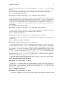
1
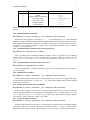
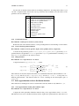
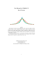
User Manual for STABLE 5.2 Excel Version Abstract This manual gives information about the STABLE library, which computes basic quantities for univariate stable distributions: densities, cumulative distribution functions, quantiles, and simulation. Statistical routines are given for fitting stable distributions to data and assessing the fit. Utility routines give information about the program and perform related calculations. Quick spline approximations of the basic functions are provided. Densities, cumulative distribution functions and simulation for discrete/quantized stable distributions are described. The multivariate module gives functions to compute bivariate stable densities, simulate stable random vectors, and fit bivariate stable data. In the radially symmetric case, the amplitude densities, cumulative distribution functions, quantiles are computed for dimension up to 100. c ⃝2002-2011 by Robust Analysis, Inc. www.RobustAnalysis.com [email protected] Revised December 13, 2010 (processed January 3, 2011) 1 STABLE User Manual 2 Contents 1 Univariate Stable Introduction 2 Univariate Stable Functions 2.1 Basic functions . . . . . . . . . . . . . . . . . . . . . . . . . . . 2.1.1 Stable densities . . . . . . . . . . . . . . . . . . . . . . . 2.1.2 Stable distribution functions . . . . . . . . . . . . . . . . 2.1.3 Stable quantiles . . . . . . . . . . . . . . . . . . . . . . . 2.1.4 Simulate stable random variates . . . . . . . . . . . . . . 2.1.5 Stable hazard function . . . . . . . . . . . . . . . . . . . 2.1.6 Derivative of stable densities . . . . . . . . . . . . . . . . 2.1.7 Second derivative of stable densities . . . . . . . . . . . . 2.1.8 Stable score/nonlinear function . . . . . . . . . . . . . . . 2.2 Statistical functions . . . . . . . . . . . . . . . . . . . . . . . . . 2.2.1 Estimating stable parameters . . . . . . . . . . . . . . . . 2.2.2 Maximum likelihood estimation . . . . . . . . . . . . . . 2.2.3 Maximum likelihood estimation with restricted parameters 2.2.4 Maximum likelihood estimation with search control . . . 2.2.5 Quantile based estimation . . . . . . . . . . . . . . . . . 2.2.6 Empirical characteristic function estimation . . . . . . . . 2.2.7 Fractional moment estimation . . . . . . . . . . . . . . . 2.2.8 Log absolute moment estimation . . . . . . . . . . . . . . 2.2.9 Quantile based estimation, version 2 . . . . . . . . . . . . 2.2.10 U statistic based estimation . . . . . . . . . . . . . . . . . 2.2.11 Confidence intervals for ML estimation . . . . . . . . . . 2.2.12 Information matrix for stable parameters . . . . . . . . . 2.2.13 Log-likelihood computation . . . . . . . . . . . . . . . . 2.2.14 Chi-squared goodness-of-fit test . . . . . . . . . . . . . . 2.2.15 Kolmogorov-Smirnov goodness-of-fit test . . . . . . . . . 2.2.16 Likelihood ratio test . . . . . . . . . . . . . . . . . . . . 2.2.17 Stable regression . . . . . . . . . . . . . . . . . . . . . . 2.3 Informational/utility functions . . . . . . . . . . . . . . . . . . . 2.3.1 Version information . . . . . . . . . . . . . . . . . . . . 2.3.2 Modes of stable distributions . . . . . . . . . . . . . . . . 2.3.3 Set internal tolerance . . . . . . . . . . . . . . . . . . . . 2.3.4 Get internal tolerance . . . . . . . . . . . . . . . . . . . . 2.3.5 Convert between parameterizations . . . . . . . . . . . . 2.3.6 Omega function . . . . . . . . . . . . . . . . . . . . . . . 2.4 Series approximations to basic distribution functions . . . . . . . 2.4.1 Series approximation of stable pdf around the origin . . . 2.4.2 Series approximation of stable cdf around the origin . . . 2.4.3 Series approximation of stable pdf at the tail . . . . . . . . 2.4.4 Series approximation of stable cdf at the tail . . . . . . . . 2.5 Faster approximations to basic functions . . . . . . . . . . . . . . 2.5.1 Quick stable density computation . . . . . . . . . . . . . 2.5.2 Quick stable cumulative computation . . . . . . . . . . . 2.5.3 Quick stable log pdf computation . . . . . . . . . . . . . 2.5.4 Quick stable quantile computation . . . . . . . . . . . . . 2.5.5 Quick stable hazard function computation . . . . . . . . . 2.5.6 Quick stable likelihood computation . . . . . . . . . . . . 2.5.7 Quick stable score/nonlinear function . . . . . . . . . . . 2.6 Discrete stable distributions . . . . . . . . . . . . . . . . . . . . . 2.6.1 Discrete stable density . . . . . . . . . . . . . . . . . . . 4 . . . . . . . . . . . . . . . . . . . . . . . . . . . . . . . . . . . . . . . . . . . . . . . . . . . . . . . . . . . . . . . . . . . . . . . . . . . . . . . . . . . . . . . . . . . . . . . . . . . . . . . . . . . . . . . . . . . . . . . . . . . . . . . . . . . . . . . . . . . . . . . . . . . . . . . . . . . . . . . . . . . . . . . . . . . . . . . . . . . . . . . . . . . . . . . . . . . . . . . . . . . . . . . . . . . . . . . . . . . . . . . . . . . . . . . . . . . . . . . . . . . . . . . . . . . . . . . . . . . . . . . . . . . . . . . . . . . . . . . . . . . . . . . . . . . . . . . . . . . . . . . . . . . . . . . . . . . . . . . . . . . . . . . . . . . . . . . . . . . . . . . . . . . . . . . . . . . . . . . . . . . . . . . . . . . . . . . . . . . . . . . . . . . . . . . . . . . . . . . . . . . . . . . . . . . . . . . . . . . . . . . . . . . . . . . . . . . . . . . . . . . . . . . . . . . . . . . . . . . . . . . . . . . . . . . . . . . . . . . . . . . . . . . . . . . . . . . . . . . . . . . . . . . . . . . . . . . . . . . . . . . . . . . . . . . . . . . . . . . . . . . . . . . . . . . . . . . . . . . . . . . . . . . . . . . . . . . . . . . . . . . . . . . . . . . . . . . . . . . . . . . . . . . . . . . . . . . . . . . . . . . . . . . . . . . . . . . . . . . . . . . . . . . . . . . . . . . . . . . . . . . . . . . . . . . . . . . . . . . . . . . . . . 5 5 5 5 5 6 6 6 6 6 6 6 7 7 7 7 7 7 8 8 8 8 8 8 9 9 9 10 10 10 10 10 11 11 11 11 11 12 12 12 12 12 12 12 13 13 13 13 13 13 STABLE User Manual 3 2.6.2 2.6.3 2.6.4 2.6.5 2.6.6 2.6.7 2.6.8 13 13 14 14 14 14 14 Quick discrete stable density . . . . . . . . . . . . . . . . . . . . . . . . . . . . . . Discrete stable cumulative distribution function . . . . . . . . . . . . . . . . . . . . Quick discrete stable cumulative distribution function . . . . . . . . . . . . . . . . . Simulate discrete stable random variates . . . . . . . . . . . . . . . . . . . . . . . . Simulate discrete stable random variates with specified saturation probability . . . . Find scale γ to have a specified saturation probability for a discrete stable distribution Discrete maximum likelihood estimation . . . . . . . . . . . . . . . . . . . . . . . 3 Multivariate Stable Introduction 4 Multivariate Stable Functions 4.1 Define multivariate stable distribution . . . . . . . . . . . . . . . . . . . . . . . . . 4.1.1 Independent components . . . . . . . . . . . . . . . . . . . . . . . . . . . . 4.1.2 Isotropic stable . . . . . . . . . . . . . . . . . . . . . . . . . . . . . . . . . 4.1.3 Elliptical stable . . . . . . . . . . . . . . . . . . . . . . . . . . . . . . . . . 4.1.4 Discrete spectral measure . . . . . . . . . . . . . . . . . . . . . . . . . . . 4.1.5 Discrete spectral measure in 2 dimensions . . . . . . . . . . . . . . . . . . . 4.1.6 Undefine a stable distribution . . . . . . . . . . . . . . . . . . . . . . . . . 4.2 Basic functions . . . . . . . . . . . . . . . . . . . . . . . . . . . . . . . . . . . . . 4.2.1 Density function . . . . . . . . . . . . . . . . . . . . . . . . . . . . . . . . 4.2.2 Cumulative function . . . . . . . . . . . . . . . . . . . . . . . . . . . . . . 4.2.3 Cumulative function (Monte Carlo) . . . . . . . . . . . . . . . . . . . . . . 4.2.4 Multivariate simulation . . . . . . . . . . . . . . . . . . . . . . . . . . . . . 4.2.5 Find a 2-dimensional rectangle with probability at least p . . . . . . . . . . . 4.3 Statistical functions . . . . . . . . . . . . . . . . . . . . . . . . . . . . . . . . . . . 4.3.1 Estimate a discrete spectral measure - fit a stable distribution to bivariate data 4.3.2 Estimate parameter functions . . . . . . . . . . . . . . . . . . . . . . . . . . 4.3.3 Fit an elliptical stable distribution to multivariate data . . . . . . . . . . . . . 4.4 Amplitude distribution . . . . . . . . . . . . . . . . . . . . . . . . . . . . . . . . . 4.4.1 Amplitude cumulative distribution function . . . . . . . . . . . . . . . . . . 4.4.2 Amplitude density . . . . . . . . . . . . . . . . . . . . . . . . . . . . . . . 4.4.3 Amplitude quantiles . . . . . . . . . . . . . . . . . . . . . . . . . . . . . . 4.4.4 Simulate amplitude distribution . . . . . . . . . . . . . . . . . . . . . . . . 4.4.5 Fit amplitude data . . . . . . . . . . . . . . . . . . . . . . . . . . . . . . . 4.4.6 Amplitude score function . . . . . . . . . . . . . . . . . . . . . . . . . . . . 4.5 Faster approximations to multivariate routines . . . . . . . . . . . . . . . . . . . . . 4.5.1 Quick log-likelihood for bivariate isotropic case . . . . . . . . . . . . . . . . 4.5.2 Quick amplitude density in bivariate case . . . . . . . . . . . . . . . . . . . 4.6 Bivariate discrete stable distribution . . . . . . . . . . . . . . . . . . . . . . . . . . 4.6.1 Discrete bivariate density . . . . . . . . . . . . . . . . . . . . . . . . . . . . 4.7 Multivariate informational/utility functions . . . . . . . . . . . . . . . . . . . . . . 4.7.1 Information about a distribution . . . . . . . . . . . . . . . . . . . . . . . . 4.7.2 Compute projection parameter functions . . . . . . . . . . . . . . . . . . . . 4.7.3 Multivariate convert parameterization . . . . . . . . . . . . . . . . . . . . . 15 . . . . . . . . . . . . . . . . . . . . . . . . . . . . . . . . . . . . . . . . . . . . . . . . . . . . . . . . . . . . . . . . . . . . . . . . . . . . . . . . . . . . . . . . . . . . . . . . . . . . . . . . . . . . . . . . . . . . . . . . . . . . . . . . . . . . 16 16 17 17 17 17 17 18 18 18 18 18 19 19 19 19 19 19 20 20 20 20 20 20 20 21 21 21 21 21 22 22 22 22 5 Error/return codes 23 References 24 Index 25 STABLE User Manual 4 1 Univariate Stable Introduction Stable distributions are a class of probability distributions that generalize the normal distribution. Stable distributions are a four parameter family: α is the tail index, or index of stability, and is in the range 0 < α ≤ 2, β is a skewness parameter and is in the range −1 ≤ β ≤ 1, γ is a scale parameter and must be positive, and δ is a location parameter, an arbitrary real number. Since there are no formulas for the density and distribution function of a general stable law, they are described in terms of their characteristic function (see below). The main purpose of the STABLE program is to make these distributions accessible in practical problems. The package enables the calculation of stable densities, cumulative distribution functions, quantiles, etc. It also can fit data by several different estimation procedures. 0.00 0.05 0.10 0.15 0.20 0.25 0.30 0.35 stable densities −4 −2 0 2 4 x Figure 1: Symmetric stable densities (β = 0) with α = 2 (Gaussian, in black), α = 1.5 (red), and α = 1 (Cauchy, green). There are numerous meanings for these parameters. We will focus on two here, which we call the 0-parameterization and the 1-parameterization. The STABLE programs use a variable param to specify which of these parameterizations to use. If you are only concerned with symmetric stable distributions, the two parameterizations are identical. For non-symmetric stable distributions, we recommend using the 0parameterization for most statistical problems, and only using the 1-parameterization in special cases, e. g. the one sided distributions when α < 1 and β = ±1. A random variable X is S(α, β, γ, δ; 0) if it has characteristic function (Fourier transform) ( [ ] ) { 1−α exp (−γ α |u|[α 1 + iβ(tan πα )(sign u)(|γu| − 1) + iδu α ̸= 1 2 ] ) E exp(iuX) = (1) 2 α = 1. exp −γ|u| 1 + iβ π (sign u) ln(γ|u|) + iδu A random variable X is S(α, β, γ, δ; 1) if it has characteristic function ] ) ( [ { )(sign u) + iδu α ̸= 1 exp (−γ α |u|[α 1 − iβ(tan πα 2 ] ) E exp(iuX) = exp −γ|u| 1 + iβ π2 (sign u) ln |u| + iδu α = 1. (2) Note that if β = 0, then these two parameterizations are identical, it is only when β ̸= 0 that the asymmetry 2 term (the imaginary factor involving tan πα 2 or π ) becomes relevant. More information on parameterizations and about stable distributions in general can be found at http://academic2.american.edu/ ∼jpnolan, which has a draft of the first chapter of Nolan (2010b). The next section gives a description of the basic univariate functions in STABLE. STABLE User Manual 5 2 Univariate Stable Functions Interfaced STABLE functions require input variables, and return the results of the computations. The interface computes the lengths of all arrays, specifies default values for some of the variables in some case, and handles return codes and results. The parameters of the stable distribution must be specified. In Excel the parameter values alpha, beta, gamma, delta, param are passed individually. The STABLE interface prints an error message when an error occurs. If an error occurs, execution is aborted; if a warning occurs, execution continues. There is basic help information built into the interfaces. In Excel, you can see the parameters to each function call in the Function Wizard, which is started by clicking on the icon fx near the top of the screen. The Excel interface requires you to select a block of cells where the output will go, and then type the function you want to compute with it’s arguments, and then press CTRL-SHIFT-ENTER (all 3 keys pressed at the same time). If you just press ENTER, you will get the error message ”You cannot change part of an array”, and Excel will lock up until you correct the entry and press CTRL-SHIFT-ENTER. For example, to simulate stable random, you select a block of cells within a column where you want the output to go, then type the command stablernd(1.7,0,1,0,0) (to simulate random variables with alpha=1.7, beta=0, gamma=1, delta=0 in the 0-parameterization), then CTRL-SHIFT-ENTER. The program then fills the number of cells that were highlighted with stable random variates. In some cases, like the multivariate elliptical routines, the output will be a block of cells with different information in them. The STABLE library is not reentrant; only one user should be using the library at once. The user should be aware that these routines attempt to calculate quantities related to stable distributions with high accuracy. Nevertheless, there are times when the accuracy is limited. If α is small, the pdf and cdf have very abrupt changes and are hard to calculate. When some quantity is small, e.g. the cdf of the light tail of a totally skewed stable distribution, the routines may only be accurate to approximately ten decimal places. There are certain values of the parameters (α near 2, α near 1, β near ±1, etc.) where there are complicated numerical problems with calculations. In these cases, the STABLE program may approximate values by rounding parameters. For example, if you try to calculate a stable pdf or cdf for α = 1.01 and β = 0.01, the STABLE program will round to α = 1 and β = 0, and compute the value for these values of the parameters. Likewise, when x is near 0 in the 1-parameterization, STABLE will do a linear interpolation to compute the pdf or cdf at that point. The thresholds used in rounding and linear approximation are described on page 11. You can manually reset these values, but be careful: the algorithms may yield poor values in some cases. The remainder of this section is a description of the functions in the STABLE library. 2.1 Basic functions 2.1.1 Stable densities Excel function: stablepdf(x,alpha,beta,gamma,delta,param) This function computes stable density functions (pdf): yi = f (xi ) = f (xi |α, β, γ, δ; param), i = 1, . . . , n. The algorithm is described in Nolan (1997). 2.1.2 Stable distribution functions Excel function: stablecdf(x,alpha,beta,gamma,delta,param) This function computes stable cumulative distribution functions (cdf): yi = F (xi ) = F (xi |α, β, γ, δ; param), i = 1, . . . , n. The algorithm is described in Nolan (1997). 2.1.3 Stable quantiles Excel function: stableinv(p,alpha,beta,gamma,delta,param) This function computes stable quantiles, the inverse of the cdf: xi = F −1 (pi ), i = 1, . . . , n. The quantiles are found by numerically inverting the cdf. Extreme tail quantiles may be hard to find because of STABLE User Manual 6 subtractive cancelation and the fact that cdf calculations may only be accurate to 10 decimal places; see the notes below. Note that the accuracy of the inversion is determined by two internal tolerances. (See Section 2.3.3.) (1) tolerance 10 is used to limit how low a quantile can be searched for. The default value is p = 10−10 : quantiles below p will be set to the left endpoint of the support of the distribution, which may be −∞. Likewise, quantiles above 1 − p will be set to the right endpoint of the support of the distribution, which may be +∞. (2) tolerance 2 is the relative error used when searching for the quantile. The search tries to get full precision, but if it can’t, it will stop when the relative error is less than tolerance 2. 2.1.4 Simulate stable random variates Excel function: stablernd(alpha,beta,gamma,delta,param) This function simulates n stable random variates: x1 , x2 , . . . , xn with parameters (α, β, γ, δ) in parameterization param. It is based on Chambers et al. (1976). The algorithm that generates stable random variates requires uniform(0,1) random variates as input. In Excel, there is an function inside STABLE that does this. That method uses two integer values as “seeds” that determine the random values produced. When you start STABLE, these seeds are always set to the same values, so unless you change them using the function stablernd seed(seed1, seed2), you will always see the same random values. If you want to “randomize” the starting seeds based on clock time, you can call stablernd seed(0,0). This will provide a different set of values for each run. If you want to repeat simulations: set the seeds manually to non-zero integers, then run your simulations. If you want to rerun the same simulations, you can reset the seeds and restart. 2.1.5 Stable hazard function Excel function: not implemented in Excel This function computes the hazard function for a stable distribution: hi = f (xi )/(1 − F (xi )), i = 1, . . . , n. 2.1.6 Derivative of stable densities Excel function: not implemented in Excel This function computes the derivative of stable density functions: yi = f ′ (xi ) = f ′ (xi |α, β, γ, δ; param), i = 1, . . . , n. 2.1.7 Second derivative of stable densities Excel function: not implemented in Excel This function computes the second derivative of stable density functions: yi = f ′′ (xi ) = f ′′ (xi |α, β, γ, δ; param), i = 1, . . . , n. 2.1.8 Stable score/nonlinear function Excel function: not implemented in Excel This function computes the score or nonlinear function for a stable distribution: g(x) = −f ′ (x)/f (x) = −(d/dx) ln f (x). The routine uses stablepdf to evaluate f (x) and numerically evaluates the derivative f ′ (x). Warning: this routine will give unpredictable results when β = ±1. The problems occur where f (x) = 0 is small; in this region calculations of both f (x) and f ′ (x) are of limited accuracy and their ratio can be very unreliable. 2.2 Statistical functions 2.2.1 Estimating stable parameters Excel function: stablefit(x,method,param) Estimate stable parameters from the data in x1 , . . . , xn , using method as described in the following table. This routine calls one of the functions described below to do the actual estimation. STABLE User Manual method value 1 2 3 4 5 6 7 7 algorithm maximum likelihood quantile empirical characteristic function fractional moment log absolute moment modified quantile U statistic method notes α ≥ 0.4 α ≥ 0.1 α ≥ 0.1 α ≥ 0.4 , β = 0, uses power p = 0.2 β=δ=0 α ≥ 0.4 β=δ=0 Note that the fractional moment and log absolute moment methods do not work when there are zeros in the data set. 2.2.2 Maximum likelihood estimation Excel function: no direct interface, use stablefit with method=1 Estimate the stable parameters for the data in x1 , . . . , xn , in parameterization param using maximum likelihood estimation. The likelihood is numerically evaluated and maximized using an optimization routine. This program and the numerical computation of confidence intervals below are described in Nolan (2001). For speed reasons, the quick log likelihood routine is used to approximate the likelihood; this is where the restriction α ≥ 0.4 comes from. 2.2.3 Maximum likelihood estimation with restricted parameters Excel function: not implemented in Excel This is a modified version of maximum likelihood estimation, where some parameters can be estimated while the others are restricted to a fixed value. The function receives theta = {alpha, beta, gamma, delta} and if restriction[i] = 1, then theta[i] is fixed; to allow a parameter to vary, set restriction[i] = 0. 2.2.4 Maximum likelihood estimation with search control Excel function: not implemented in Excel This is maximum likelihood estimation with greater control over the search and ranges for the parameters. It is used internally. 2.2.5 Quantile based estimation Excel function: no direct interface, use stablefit with method=2 Estimate stable parameters for the data in x, using the quantile based on the method of McCulloch (1986). It sometimes has problems when α is small, say α < 1/2, and the data is highly skewed. Try the modified version below in such cases. 2.2.6 Empirical characteristic function estimation Excel function: no direct interface, use stablefit with method=3 Estimate stable parameters for the data in x using the empirical characteristic function based method of Koutrovelis-Kogon-Williams, described in Kogon and Williams (1998). An initial estimate of the scale gamma0 and the location delta0 are needed to get accurate results. We recommend using the quantile based estimates of these parameters as input to this routine. 2.2.7 Fractional moment estimation Excel function: no direct interface, use stablefit with method=4 Estimate stable parameters for the data in x, using the fractional moment estimator as in Nikias and Shao (1995). This routine only works in the symmetric case, it will always return β = 0 and δ = 0. In this case the 0-parameterization coincides with the 1-parameterization, so there is no need to specify parameterization. p STABLE User Manual 8 is the fractional moment power used. A reasonable default value is p = 0.2; take p < α/2 to get reasonable results. This method does not work if there are zeros in the data set - negative sample moments do not exist. Remove zero values (and possibly values close to 0) from the data set if you want to use this method. 2.2.8 Log absolute moment estimation Excel function: no direct interface, use stablefit with method=5 Estimate stable parameters for the data in x, using the log absolute moment method as in Nikias and Shao (1995). This routine only works in the symmetric case, it will always return β = 0 and δ = 0. In this case the 0-parameterization coincides with the 1-parameterization, so there is no need to specify parameterization. The log absolute moment method does not work when there are zeros in the data set, because log |x| is undefined when x is 0. Remove zero values (and possibly values close to 0) from the data set if you want to use this method. 2.2.9 Quantile based estimation, version 2 Excel function: no direct interface, use stablefit with method=6 Estimate stable parameters for the data in x, using a modified quantile method of Nolan (2010b). It should work for any values of the parameters, but some extreme values are inaccurate. 2.2.10 U statistic based estimation Excel function: no direct interface, use stablefit with method=7 Estimate stable parameters for the data in x, using the method of Fan (2006). It only works for the symmetric case. 2.2.11 Confidence intervals for ML estimation Excel function: stablefitmleci(theta,z,n,sigtheta) This routine finds confidence intervals for maximum likelihood estimators of all four stable parameters. The routine returns a vector sigtheta of half widths of the confidence interval for each parameter in theta=(alpha,beta,gamma,delta). These values depend on the confidence level you are seeking, specified by z, and the size of the sample n. The z value is the standard critical value from a normal distribution, i.e. use z = 1.96 for a 95% confidence interval. For example, the point estimate of α is theta[1], and the confidence interval is theta[1]±sigtheta[1]. For β, the confidence interval is theta[2]±sigtheta[2], for γ, the confidence interval is theta[3]±sigtheta[3], For δ, the confidence interval is theta[4] ± sigtheta[4]. These values do not make sense when a parameter is at the boundary of the parameter space, e.g. α = 2 or β = ±1. These values are numerically approximated using a grid of numerically computed values in Nolan (2001). The values have limited accuracy, especially when α ≤ 1. 2.2.12 Information matrix for stable parameters Excel function: not implemented in Excel Returns the 4 × 4 information matrix for maximum likelihood estimation of the stable parameters for parameter values theta. This is done in the continuous 0-parameterization. These are approximate values, interpolated from a grid of numerically computed values in Nolan (2001) for α ≥ 0.5. The values have limited accuracy, especially when α ≤ 1. 2.2.13 Log-likelihood computation Excel function: not implemented in Excel Compute the log-likelihood of the data, assuming an underlying stable distribution with the specified STABLE User Manual 9 parameters. 2.2.14 Chi-squared goodness-of-fit test Excel function: not implemented in Excel Compute chi-squared goodness-of-fit statistic for the data in x1 , . . . , xn using nclass equally probable classes/bins. 2.2.15 Kolmogorov-Smirnov goodness-of-fit test Excel function: not implemented in Excel This function computes the Kolmogorov-Smirnov two-sided test statistic: D= sup −∞<x<∞ |F (x) − F̂ (x)|, where F (·) is the stable cdf with parameters α = theta[1], β = theta[2], γ = theta[3], δ = theta[4] and F̂ (·) is the sample cdf of the data in x. Use method=0 for quick computations (stableqkcdf is used to compute cdf), use method=1 for slower computations (stablecdf is used to compute cdf). The routine returns the observed value of D and an estimate of the tail probability P (D > d), i.e. the significance level of the test. This tail probability is calculated using Stephen’s approximation to the limiting distribution, e.g. (n1/2 + 0.12 + 0.11n−1/2 )D is close to the limiting Smirnov distribution. This is close to n1/2 D for large n, and a better approximation on the tails for small n. Note, this calculation is not very accurate if the tail probability is large, but these cases aren’t of much interest in a goodness-of-fit test. (If you don’t like this approximation, the function returns D, and you can compute your own tail probability.) WARNING: the computation of the significance level is based on the assumption that the parameter values theta=(α, β, γ, δ) were chosen independently of the data. If the parameters were estimated from the data, then this tail probability will be an overestimate of the significance level. 2.2.16 Likelihood ratio test Excel function: not implemented in Excel This function computes the likelihood ratio L0 /L1 , where L0 is the maximum likelihood of the data x under the assumption that x is an i.i.d. sample from a stable distribution with α and β restricted to the range abnd[1] ≤ α ≤ abnd[2] and bbnd[1] ≤ β ≤ bbnd[2], and L1 is the maximum likelihood of the data under an unrestricted stable model. The function computes the maximum likelihood using the quick approximation to stable likelihoods, so is limited to α in the range [0.4,2]. The vector results will contain the results of the computations: results[1] = ratio of the likelihoods results[2] = -2*log(ratio of likelihoods) results[3] = log likelihood of the data for the restricted H0 results[4] = log likelihood of the data for the unrestricted H1 results[5] = estimated value of alpha under H0 results[6] = estimated value of beta under H0 results[7] = estimated value of gamma under H0 results[8] = estimated value of delta under H0 results[9] = estimated value of alpha without assuming H0 results[10] = estimated value of beta without assuming H0 results[11] = estimated value of gamma without assuming H0 results[12] = estimated value of delta without assuming H0 Note that under the standard assumptions, results[2] converges to a chi-squared distribution with d.f. = (# free parameters in H1 parameter space - # free parameters in H0 parameter space) as the sample size tends to ∞. For example, to compute the likelihood ratio test for the null hypothesis H0: data comes from a normal distribution vs H1: data comes from stable distribution, use abnd=(2,2) and bbnd=(0,0), in which case STABLE User Manual 10 results[2] will have 2 d.f. To test H0: data comes from a symmetric stable distribution vs H1: data comes from a general stable distribution, use abnd=(0.4,2) and bbnd=(0,0), in which case results[2] will have 3 d.f. 2.2.17 Stable regression Excel function: stableregression(x,trimprob,theta init,theta trim,theta, symmetric) Computes linear regression coefficients θ1 , θ2 , . . . , θk for the problem yi = θ1 xi,1 + θ2 xi,2 + · · · + θk xi,k + ei , i = 1, . . . , n where the error term ei has a stable distribution. In matrix form, the equation is y = Xθ + e. The algorithm uses maximum likelihood and is described in Nolan and Ojeda (2010). y is a vector of length n of observed responses. x is a n × k matrix, with the columns of x representing the variables and the rows representing the different observations. NOTE: if you want an intercept term, you must include a column of ones in the x matrix. Typically one sets the first column of x to ones, and then θ1 is the intercept. trimprob is a vector of length 2, e.g. (0.1,0.9), which gives the lower and upper quantiles for the trimmed regression. (Trimmed regression trims off extreme values and then performs ordinary least squares regression. The resulting coefficients are used to get an initial estimate of the stable regression coefficients.) symmetric can be used to force the fitting program to assume symmetry in the error terms ei . The interfaced versions of this function returns a structure with different fields. • theta is the vector of coefficients • theta init is the initial vector of coefficients from the OLS regression • theta trim is the initial vector of coefficients from the trimmed regression • alpha,beta,gamma are the stable parameters estimated from the residuals. They can be regarded as nuisance parameters if you only care about the coefficients. Note that all parameters are in the 2-parameterization. You can convert to another representation using the convert parameterization function in Section 2.3.5. It is assumed that the location parameter δ is zero. Note that in the non-Gaussian stable case, some of the traditional assumptions in regression are no longer true. In particular, it is NOT always the case that Eei = 0. First, if α ≤ 1, the heavy tails will mean that Eei is undefined. Second, in the non-symmetric case, for β ̸= 0, we do not require Eei = 0. Instead, the regression uses the 2-parameterization so that the mode of ei is zero. The reason for this is to make the regression line go through the center of the data points. 2.3 Informational/utility functions 2.3.1 Version information Excel function: stableversion stableversion( ) returns a string with version information. 2.3.2 Modes of stable distributions Excel function: not implemented in Excel Returns the mode of a S(α = theta[1], β = theta[2], γ = theta[3], δ = theta[4]; param) distribution. If β ̸= 0, the mode is determined by a numerical search of the pdf. 2.3.3 Set internal tolerance Excel function: stablesettolerance(inum,value) STABLE User Manual 11 Sets the value of internal tolerances that are used during computations. You change these values at your own risk: computation times can become very long, inaccuracy can accumulate, and some choices of the parameters can cause infinite loops. inum 0 1 2 3 4 5 6 7 8 9 10 11 meaning relative error for pdf numerical integration relative error for cdf numerical integration relative error for quantile search alpha and beta rounding x tolerance near zeta exponential cutoff peak/strim location tolerance stabletrim tolerance minimum alpha minimum xtol threshold for quantile search x tolerance 2.3.4 Get internal tolerance Excel function: stablegettolerance(inum,value) Returns the value of the internal tolerances, see the preceding function for the meanings of each variable. 2.3.5 Convert between parameterizations Excel function: stableconvert(param,alpha,beta,gamma,delta,newparam) Convert from the parameters given in theta=(alpha,beta,gamma,delta) given in the paramparameterization to the parameters thetanew given in the newparam-parameterization. Currently param and newparam are restricted to the values 0,1,2 and 3. 2.3.6 Omega function Excel function: not implemented in Excel Compute the function ω(ui |α, β; k), i = 1, . . . , n where ] { α[ 1−α |u| [ 1 + iβ(tan πα − 1) α ̸= 1 2 )(sign]u)(|u| ω(u|α, β; 0) = |u| 1 + iβ π2 (sign u) ln |u| α = 1, ] { α[ πα |u| [ 1 − iβ(tan 2 )(sign]u) α ̸= 1 ω(u|α, β; 1) = |u| 1 + iβ π2 (sign u) ln |u| α = 1. (3) These functions are from the characteristic functions of standardized univariate stable distributions: if Z ∼ S (α, β, 1, 0; k), then E exp(iuZ) = exp(−ω(u|α, β; k)). As before, k = 0 or k = 1 correspond to two different parameterization. The function returns two vectors containing the real and imaginary parts of ω(u|α, β; k) 2.4 Series approximations to basic distribution functions These functions use the Bergstrom series for stable densities and cdfs, which are only defined for α ̸= 1. 2.4.1 Series approximation of stable pdf around the origin Excel function: not implemented in Excel Computes the stable probability distribution function using a series approximation with nterms in it. This function is best used to calculate the density near the origin in the 1-parameterization. The series is not STABLE User Manual 12 defined for α = 1. Note that nterms=1 corresponds to a constant term, nterms=2 corresponds to a linear term, etc. 2.4.2 Series approximation of stable cdf around the origin Excel function: not implemented in Excel Computes the stable cumulative distribution function using a series expansion with nterms in it. This function is best used to calculate the cdf near the origin in the 1-parameterization. The series is not defined for α = 1. Note that nterms=1 corresponds to a constant term, nterms=2 corresponds to a linear term, etc. 2.4.3 Series approximation of stable pdf at the tail Excel function: not implemented in Excel Computes the stable probability distribution function using a series approximation with nterms in it. This function is best used to calculate points on the tail of a distribution. The series is defined only for x > 0. (For x < 0, replace x by −x and β by −β. The series is not defined for α = 1. 2.4.4 Series approximation of stable cdf at the tail Excel function: not implemented in Excel Computes the stable cumulative distribution function using a series approximation with nterms in it. This function is best used to calculate points on the tail of a distribution. The series is defined only for x > 0. (For x < 0, replace x by −x and β by −β. The series is not defined for α = 1. 2.5 Faster approximations to basic functions The functions described in preceding sections are accurate, but can take a long time to compute. For evaluating a single pdf or cdf at a single set of parameter values, they are fine. However, when the functions must be evaluated many times, the previous routines are slow. For example, when estimating stable parameters by maximum likelihood estimation, the likelihood is evaluated at each data point for a large number of parameter values during the numerical search for the point where the likelihood is maximized. In these cases, speed is more desirable than great accuracy. The functions described below are approximations to the functions above, and are based on pre-computed values using those basic functions. They are designed to evaluate the quantity of interest at many x values for fixed values of α and β. Each routine has a setup time, and if you change α or β, that setup code must be rerun. It can be slower to run these routines than the basic routines above if you only want to calculate the quantity at a few x values. These routines work for 0.2 ≤ α ≤ 2 and all −1 ≤ β ≤ 1. 2.5.1 Quick stable density computation Excel function: stableqkpdf(x,alpha,beta,gamma,delta,param) Call is identical to Section 2.1.1, results are approximately the same. 2.5.2 Quick stable cumulative computation Excel function: stableqkcdf(x,alpha,beta,gamma,delta,param) Call is identical to Section 2.1.2, results are approximately the same. 2.5.3 Quick stable log pdf computation Excel function: not implemented in Excel STABLE User Manual 13 Approximates log(pdf) for stable distributions. Results are approximately the same as log(f (x)). 2.5.4 Quick stable quantile computation Excel function: stableqkinv(p,alpha,beta,gamma,delta,param) Call is identical to Section 2.1.3, but much faster. Note the comments in that section about extreme upper quantiles. 2.5.5 Quick stable hazard function computation Excel function: Not implemented in Excel Call is identical to Section 2.1.5. 2.5.6 Quick stable likelihood computation Excel function: Not implemented in Excel Call is identical to Section 2.2.13. 2.5.7 Quick stable score/nonlinear function Excel function: Not implemented in Excel This function approximates the score or nonlinear function for a stable distribution: g(x) = −f ′ (x)/f (x) = −(d/dx) ln f (x). The algorithm used depends on the value of method. When method=1, stableqkpdf is used to compute f (x) and in the numerical evaluation of f ′ (x). When method=2, stablescorefn is used to compute g(x) on a grid, then a spline is fit to those values. The resulting spline is used to approximate g(x). If n is large, this is noticeably faster than either stablescorefn or method=1 above. When method=3, a rational function approximation is used to approximate g(x). This is the fastest method, but the accuracy depends on the values of alpha and beta. If alpha is between 1 and 1.9 and beta is near 0, the approximation is good. 2.6 Discrete stable distributions Given a stable distribution X ∼ S(α, β, γ, δ; param) and a pair of cutoff values a < b, the random variable Y = integer part of max(a, min(X, b)) is a discrete stable distribution. These distribution arise in signal processing where a continuous quantity is quantized/digitized and limited accuracy is kept. It is assumed that the cutoff values are integers. The saturation probability is P (X < a − 1/2) + P (X > b + 1/2), and is a measure of how much of the distribution is lost by truncating at the cutoff values. In the routines below, the cutoff is specified by a vector of length 2: cutoff=(a, b). In this section X will always refer to the continuous stable distribution, while Y will always refer to a discrete/quantized/integer valued distribution. In the internal routines, the x values are integers. The matlab/R/Mathematica interfaces use double precision values. 2.6.1 Discrete stable density Excel function: Not implemented in Excel Calculates fi = P (Y = xi ), i = 1, . . . , n. 2.6.2 Quick discrete stable density Excel function: Not implemented in Excel Calculates fi = P (Y = xi ), i = 1, . . . , n. Faster than above, less accurate. 2.6.3 Discrete stable cumulative distribution function Excel function: Not implemented in Excel STABLE User Manual 14 Calculates Fi = P (Y ≤ xi ), i = 1, . . . , n. 2.6.4 Quick discrete stable cumulative distribution function Excel function: Not implemented in Excel Calculates Fi = P (Y ≤ xi ), i = 1, . . . , n. Faster than above, less accurate. 2.6.5 Simulate discrete stable random variates Excel function: Not implemented in Excel Simulates discrete stable random variates with the specified parameters and cutoffs. 2.6.6 Simulate discrete stable random variates with specified saturation probability Excel function: Not implemented in Excel Simulates discrete stable random variates, where the scale is computed internally to make the saturation probability=psaturation. Note that in cases where the stable parameters are passed individually, gamma is NOT used. In the cases where the vector theta is used, the value of γ =theta[3] is ignored. The following function is used to compute γ, then the previous function is called to generate the values. 2.6.7 Find scale γ to have a specified saturation probability for a discrete stable distribution Excel function: Not implemented in Excel Given α, β, δ and cutoff= (a, b), the scale γ is computed to get the requested saturation probability, e.g. psaturation=P (X < a − 1/2) + P (X > b + 1/2). 2.6.8 Discrete maximum likelihood estimation Excel function: Not implemented in Excel Estimate the stable parameters for the discrete stable data in x1 , . . . , xn , in parameterization param using maximum likelihood estimation. The likelihood is numerically evaluated and maximized using an optimization routine. When method=1, stablepdfdiscrete is used to calculate likelihood, when method=2, symmetry is assumed (β = 0) and a faster method is used to compute the likelihood. STABLE User Manual 15 3 Multivariate Stable Introduction WARNING: The Excel interface for multivariate stable distributions currently only implements two functions: mvstablerndelliptical( ) and mvstablefitelliptical( ). To specify a multivariate stable distribution X = (X1 , X2 , . . . , Xd )T in d dimensions requires an index of stability α ∈ (0, 2], a finite Borel measure Λ on the unit sphere S = {s ∈ Rd : |s| = 1} and a shift vector δ ∈ Rd . The measure Λ is called the spectral measure of the distribution. The joint characteristic function of X ∼ S (α, Λ, δ; k) is given by: ) ( ∫ E exp(i < u, X >) = exp − ωk (< u, s > |α, 1; k)Λ(ds) + i < u, δ > , S where ω(u|α, β; k) is defined in (3). As in one dimension, the 1-parameterization is more common in theoretical research, while the 0-parameterization is better suited to computation and statistical problems. Here and below, < u, X >= uXT = u1 X1 + · · · + ud Xd is the inner product. Symmetric stable distribud tions are defined by the condition X= − X, which is equivalent to Λ being a symmetric measure on S, i.e. Λ(A) = Λ(−A) for any Borel subset A ⊂ S. As in the univariate case, in the symmetric case the 0=parameterization and the 1-parameterization coincide. The general case is beyond current computational capabilities, but several special cases: isotropic (radially symmetric), elliptical, independent components and discrete spectral measure are computationally accessible. isotropic The spectral measure is continuous and uniform, leading to isotropic/radial symmetry for the distribution. The characteristic function is E exp(i < u, X >) = exp (−γ0α |u|α + i < u, δ >) . (4) elliptical The characteristic function is ( ) E exp(i < u, X >) = exp −(uT Ru)(α/2) + i < u, δ > (5) where R is a positive definite matrix. (R = γ02 I is equivalent to the isotropic case above.) More information on this accessible class of distributions is given in Nolan (2010a). independent components If components are independent with Xj ∼ S (α, βj , γj , δj ; k), then the characteristic function is d ∑ E exp(i < u, X >) = exp − ω(uj |α, βj ; k)γjα + i < u, δ > (6) j=1 This is a special case of the discrete spectral measure below: the spectral mass is concentrated on the points where the coordinates axes intersect the unit sphere. discrete When the spectral measure is discrete with mass λj at sj ∈ S, j = 1, . . . , m the characteristic function is m ∑ E exp(i < u, X >) = exp − ω(< u, sj > |α, 1; k)λj + i < u, δ > (7) j=1 This discrete class is dense in the class of all stable distributions: any finite spectral measure Λ can be approximated by a discrete measure, see Byczkowski et al. (1993). Below is a plot of the density surface of a bivariate stable density with three point masses, each of weight 1 at locations (cos(π/3), sin(π/3)), (-1,0), and (cos(5π/3), sin(5π/3)) STABLE User Manual 16 density surface triangle, alpha=1.3 0.01 1 2 Z 1 2 3 04 .05 0 0.0 0.0 0.0 0. 0 3 contours of density surface 0.02 0.04 0 xx 0.03 3 1 2 -1 -1 -2 0 X -3 -3 -3 -2 3 1 -2 0 Y -1 2 0.01 0.01 -3 -2 -1 0 1 2 3 xx 4 Multivariate Stable Functions Since the specification of a multivariate stable distribution is somewhat cumbersome, a different approach from the univariate case is taken in these routines. Two steps are needed to work with a multivariate stable distribution. First, the distribution is specified by calling a function to define the distribution. Second, call a separate functions to compute densities, cumulatives, simulate, etc. The programs for working with multivariate stable distributions are less well developed and generally limited to 2 dimensions. At the current time, when dimension 2 < d ≤ 100, you can: • simulate using mvstablernd • fit multivariate data with an elliptical model • calculate the pdf using mvstablepdf if the components are independent OR the spectral measure has exactly d point masses OR the distribution is isotropic or elliptical • calculate the cdf using mvstablecdf if the components are independent • calculate the cdf using mvstablecdfMC by Monte Carlo estimation for any type of distribution The accuracy of the multivariate pdf and cdf calculations are limited. In all cases, X is a column vector, this is important to remember when you specify x for calculating the multivariate pdf or cdf. 4.1 Define multivariate stable distribution STABLE has the ability to work with multiple distributions. When a multivariate stable distribution is defined, a ‘distribution descriptor’ is returned. That descriptor must be used when computing quantities for that STABLE User Manual 17 distribution. Note: The descriptor should not be changed by a user. The descriptor may change between calls, and contents may vary in future versions of STABLE. There are different functions used to define each of the different types of distributions that STABLE can work with. They are described below. 4.1.1 Independent components Excel function: Not implemented in Excel Define a multivariate stable distribution with dimension d≤ 100 and independent components with characteristic function (6). beta, gamma and delta should be vectors of length d= the dimension of the distribution. 4.1.2 Isotropic stable Excel function: Not implemented in Excel Define a multivariate isotropic stable distribution with with dimension d≤ 100 and characteristic function (4). d is the dimension of the distribution, gamma0 is the scale parameter, delta is the location vector. 4.1.3 Elliptical stable Excel function: Not implemented in Excel Define a multivariate elliptically contoured/sub-Gaussian stable distribution with dimension d≤ 100 and with characteristic function (5). The dimension of the distribution is determined from the size of R, a positive definite d × d shape matrix, and delta is the location vector. 4.1.4 Discrete spectral measure Excel function: Not implemented in Excel Define a multivariate stable distribution with discrete spectral measure with dimension d≤ 100 and characteristic function (7). s should be a d × nlambda matrix specifying the location of the point masses as columns, lambda should be a row vector of length nlambda containing the weights. beta should be a row vector of length nlambda specifying the skewness at each point mass. delta is the shift as a column vector. param is the parameterization, must be 0 or 1. The spectral measure is defined by putting mass lambda[j]*(1+beta[j])/2 at sj and mass lambda[j]*(1beta[j])/2 at −sj . Setting all beta equal to 1 gives the standard definition of a spectral measure, with mass lambda[j] at s[j]. Setting all beta equal to 0 guarantees that the distribution is symmetric, putting weight lambda[j]/2 at ±sj . If any element of beta is not 0, the distribution is assumed to be nonsymmetric. (It is possible to manually make a spectral measure symmetric with nonzero beta by defining antipodal points and weights and values of beta that balance correctly. However, STABLE does not detect this.) Some parts of STABLE are significantly faster and more accurate in the symmetric case, e.g. density calculations and simulations. 4.1.5 Discrete spectral measure in 2 dimensions Excel function: Not implemented in Excel Define a bivariate stable distribution with discrete spectral measure. This is a special case of the previous function. In two dimensions the locations of the point masses can be specified by angles: angle[j] gives the angle (in radians) of the location of sj = (cos(angle[j]), sin(angle[j])). There are several special cases that are handled differently internally: • When angle and lambda are of length 2, densities can be calculated in terms of univariate densities. • The special case of the previous one is when angle=(0, π/2). This corresponds to a distribution with independent components. Both density and cdf are calculated in terms of products of univariate density and cdf respectively. STABLE User Manual 18 • If all elements of beta are 0, the distribution is symmetric. Cumulative distribution function calculations only work in the symmetric case (though Monte Carlo based cdf estimation works for any case you can simulate, including skewed.) 4.1.6 Undefine a stable distribution Excel function: Not implemented in Excel Clears the definition of the stable distribution dist. When a multivariate stable distribution is defined by one of the above functions, the STABLE library allocates memory for a distribution descriptor. The amount of memory used is not large, and this should not normally be a problem. But if your program loops and defines many multivariate stable distributions, you could have a memory problem as the descriptors accumulate. Calling this function when you are done with a stable distribution will deallocate the memory. A technical detail: distribution descriptors are allocated internally in the STABLE library, not in the workspace of the user session. If you exit, these distribution descriptors are lost, EVEN IF YOUR SESSION INFORMATION IS SAVED. You must redefine all multivariate distributions when you restart the STABLE library. 4.2 Basic functions 4.2.1 Density function Excel function: Not implemented in Excel Computes the density f (x) for stable distribution dist at each value in x. Note: this routine assumes that the density exists. The density will not exist if the spectral measure is supported on a proper linear subspace of the domain. When dimension d > 2, the pdf can be calculated in special cases: • the components are independent components • the spectral measure is discrete AND the number of point masses is equal the dimension of the problem • the isotropic case • the elliptical case Otherwise, only 2-dimensional computations can be done. The symmetric case uses the method in Abdul-Hamid and Nolan (1998), the nonsymmetric case uses the method in Nolan and Rajput (1995). The symmetric case is faster and more accurate than the nonsymmetric case. Both routines are accurate near the center of the distribution, and have limited accuracy near the tails. 4.2.2 Cumulative function Excel function: Not implemented in Excel This function approximates P (a ≤ X ≤ b). If the components are independent, this works in dimensions up to 100. In the symmetric two-dimensional case, the probability is evaluated by numerically integrating the (numerically computed) 2-dimensional density f (x). Due to the limited precision in the numerical calculation of the density, and the approximate nature of the integration of this density, this routine gives only a few digits of accuracy. To find the probability of an unbounded regions, it is best to truncate the region using the routine in Section 4.2.5 to find a bounded rectangle containing most of the probability. Use the function in Section 4.2.3 to approximate in 2-dimensional nonsymmetric case or in higher dimensions. 4.2.3 Cumulative function (Monte Carlo) Excel function: Not implemented in Excel STABLE User Manual 19 This function approximates P (a ≤ X ≤ b) by simulating n indepedent random vectors with the same distribution as X and counting how many are in the interval [a, b]. It works for any distribution and dimension that can be simulated. 4.2.4 Multivariate simulation Excel function: mvstablerndellptical(alpha,delta,R) In Excel, one can only simulate from a multivariate elliptical distribution. To do this, specify the stable index alpha, a location vector delta (length d), and a shape matrix R (a d × d matrix). The output should be a block of n × d columns, where n is the number of values to simulate. 4.2.5 Find a 2-dimensional rectangle with probability at least p Excel function: Not implemented in Excel Find a number r so that the 2-dimensional rectangle A = A(r) = [−r, r] × [−r, r] has P (X ∈ A) ≥ p, where X is a bivariate stable distribution defined by dist. This is used for technical calculations, e.g. in approximating the probability of unbounded regions. The method uses univariate projections and will generally give an overestimate of r. The method is less accurate for small p or if the distribution is not centered or highly skewed, it gets more accurate if p is close to 1 and the distribution is centered and symmetric. If p is not too close to 1, one can get a better value of r by making repeated calls to the multivariate cdf function with rectangles of the form A(r) and search for a value of r that makes P (X ∈ A(r)) close to p. That procedure involves bivariate numerical integration will take much longer than this function. 4.3 Statistical functions 4.3.1 Estimate a discrete spectral measure - fit a stable distribution to bivariate data Excel function: Not implemented in Excel x contains the data values, nspectral is the number of points in the estimated spectral measure (must be divisible by 4), method1d is the method to use for estimating univariate stable parameters internally (see Section 2.2.1 for codes; only used if method2d=1), method2d is the method to use in estimating bivariate distribution. Use method2d=1 for Rachev-Xin-Cheng method, method2d=2 for projection method, method2d=3 for empirical characteristic function method. The methods are described in Nolan et al. (2001), see Nolan and Panorska (1997) for some discussion of suggested values and diagnostics. Suggest using nspectral=40, method1d=3, method2d=2, param=1. The function returns a list/structure that contains information about the fit, which is always done as a discrete spectral measure. The fields in the fit are: the estimated value of α, the estimated shift/location vector δ, angle which is a uniform grid from 0 to 2π of length nspectral, and lambda for the estimated weights at each position. 4.3.2 Estimate parameter functions Excel function: Not implemented in Excel Estimate the parameter functions for the bivariate data in x. The data is projected in each direction given by angle and the parameters are estimated in the param parameterization. method1d is the univariate method used to estimate the parameters (see Section 2.2.1 for codes). The result is a matrix of dimension length(x)×5. The columns of the result are (1) for the angle, (2) for the estimate of α, (3) for the estimate of β, (4) for the estimate of γ, (5) for the estimate of δ at that angle. 4.3.3 Fit an elliptical stable distribution to multivariate data Excel function: mvstablefitelliptical(x,method1d) x contains the data values (d-vectors), method1d is the method to use for estimating univariate stable parameters internally (see Section 2.2.1 for codes). STABLE User Manual 20 The output should be a block of cells with d rows and d + 2 columns. The first column will have the estimated alpha in the first row (and no other entries). The second column will have the estimated shift vector delta. The remaining columns will contain an estimate of the d × d shape matrix R. 4.4 Amplitude distribution For d-dimensional random vector X, the univariate quantity R = |X| is called the amplitude of X. When X is isotropic, the radial symmetry allows one to reduce the dimension of the problem to a univariate problem. The following routines compute the cdf, pdf, quantiles, simulate and estimate for amplitudes of isotropic stable random vectors. Since these are univariate quantities, and it is required that the distribution is isotropic, one does NOT have to define the isotropic distribution separately. Because of computational difficulties, these routines are limited to dimension d ≤ 100. 4.4.1 Amplitude cumulative distribution function Excel function: Not implemented in Excel Compute the cdf of the amplitude distribution: FR (r) = P (R ≤ r) for R = |X|, where X is an d dimensional isotropic stable random vector with characteristic function E exp(i < u, X >) = exp(−γ0α |u|α ). Current implementation works for α ∈ [0.8, 2]. There seems to be a relative error of approximately 3% for large r. 4.4.2 Amplitude density Excel function: Not implemented in Excel Compute the density fR (r) where R is described above. Current implementation works for α ∈ [0.8, 2]. There seems to be a relative error of approximately 3% for large r. 4.4.3 Amplitude quantiles Excel function: Not implemented in Excel Compute the quantiles of the amplitude R described above. Current implementation works for α ∈ [0.8, 2]. 4.4.4 Simulate amplitude distribution Excel function: Not implemented in Excel Simulate n i.i.d. values of the amplitude distribution R as described above. Current implementation works for α ∈ (0.2, 2]. 4.4.5 Fit amplitude data Excel function: Not implemented in Excel Estimate the parameters α and γ0 for amplitude data. r contains the (univariate) amplitude data values, d is the dimension of the underlying distribution that the amplitude data comes from, method is the method to use for estimating. This initial implementation allows only method=5, which uses method of moments on the log of the amplitude data. Other methods are planned for the future. The function returns the estimated value of α and γ0 . 4.4.6 Amplitude score function Excel function: Not implemented in Excel Compute the score function of the amplitude: g(r) = −f ′ (r)/f (r), where f (r) = fR (r|α, γ0 , d) is the amplitude pdf defined above. Current implementation works for α ∈ [0.8, 2], d ≤ 98. There seems to be a STABLE User Manual 21 relative error of approximately 3% for large r. 4.5 Faster approximations to multivariate routines There are a limited number of functions for quickly calculating multivariate functions in the 2-dimensional isotropic case. Such a distribution is specified by the index of stability α, the scale γ0 , and the location δ = (δ1 , δ2 ). Because the description is simple, these functions use those arguments directly and do not use a distribution descriptor. 4.5.1 Quick log-likelihood for bivariate isotropic case Excel function: Not implemented in Excel Compute the log likelihood of the bivariate isotropic stable data in x with stable index alpha, scale gamma0, and location vector delta. An internal approximation is used to compute the single value ℓ(α, γ0 , δ|x1 , . . . , xn ) = log n ∏ fX (xi |α, γ0 , δ). i=1 This function is designed to compute the log likelihood for a fixed α many times. In this case, it is much faster than trying to compute the right hand side above using the bivariate pdf routine in Section 4.2.1. It is also more accurate than that routine, especially on the tails. The program initially computes an approximation that depends on α; if α changes, the approximation must be recomputed and it will be slower. 4.5.2 Quick amplitude density in bivariate case Excel function: Not implemented in Excel Compute the amplitude function fR (r|α, γ0 , d = 2) for a 2-dimensional isotropic stable vector . For large n, it is much faster than the function in Section 4.4.2. 4.6 Bivariate discrete stable distribution A bivariate discrete stable distribution is defined by digitizing and truncating a continuous bivariate stable distribution X = (X1 , X2 )T : discrete Y = (Y1 , Y2 )T has components Yi = integer part of max(a, min(Xi , b)), where cutoff=(a, b) are the upper and lower cutoff values. Note that the same cutoff is used for both components of X. These distributions arise in signal processing where a bivariate continuous quantity is quantized/digitized and limited accuracy is kept. It is assumed that the cutoff values are integers. The saturation probability is psat = P (X1 < a − 1/2) + P (X1 > b + 1/2) + P (X2 < a − 1/2) + P (X2 > b + 1/2), and is a measure of how much of the distribution is lost by truncating at the cutoff values. In the internal routines, the x values are integers. The R, Mathematica and matlab interfaces store these integer values in double precision numbers. 4.6.1 Discrete bivariate density Excel function: Not implemented in Excel Compute the pdf of a discrete bivariate stable distribution. x should be a 2 × n matrix of integer values, cutoff is a vector of length 2 with upper and lower cutoff values for the truncation. The typical value for cutoff is (-128,127); both components of (X1 , X2 ) are truncated at the same value. The function returns a vector p of length n with pi = P (Y = xi ) = P (Y1 = x1i , Y2 = x2i ). Note that eps is the attempted accuracy for each probability pi , not for the total error. The probabilities are computed using the bivariate cdf function above and thus only works for symmetric stable two dimen∑ sional distributions. It’s accuracy is limited: it is likely that when all possible values of x are used, i pi STABLE User Manual 22 will be slightly different from 1. The current implementation is slow. The method variable is unused at the current time; it will be used for faster approximations in future implementations. 4.7 Multivariate informational/utility functions 4.7.1 Information about a distribution Excel function: Not implemented in Excel Returns information about distribution dist. Useful for checking that definition. 4.7.2 Compute projection parameter functions Excel function: Not implemented in Excel Compute the exact parameter functions for a bivariate stable distribution. For direction t ∈ R2 , (X, tj ) is univariate stable with parameters (α, β(t), γ(t), δ(t)). This function computes the parameter functions β(·), γ(·) and δ(·) at the values t = (cos angle[j], sin angle[j]). Angles in angle are given in radians. 4.7.3 Multivariate convert parameterization Excel function: Not implemented in Excel Converts between multivariate stable parameterizations. newparam must be 0 or 1. In the interfaced versions of STABLE, the input distribution dist is converted to the new parameterization, and a new distribution descriptor is returned. STABLE User Manual 23 5 Error/return codes An error is unrecoverable and stops execution. For example, if you ask to compute the density of a stable parameter with α = 3, you will get a return code of 1 and your function will stop. In contrast, a warning is informational and is usually not serious. It alerts you to the fact that the results of a calculation may have some inaccuracy. For example, stable densities have radical changes of the tail behavior when α = 2 or β = ±1, and the computations have small inaccuracies in them. In practical terms this usually means little, as the difference between an α = 1.99 stable distribution and an α = 2 stable distribution in an statistical problem is likely to be unobservable in practice. Return codes for STABLE program are given in the tables below. Univariate routines return error codes in the range 1-99, multivariate routines return error codes in the range 100-199. code 0 1 2 3 4 5 6 7 8 9 10 11 12 13 14 15 16 17 18 19 20 21 30 type error error error error warning warning warning warning error error error error error error error error error error error error error error meaning No error Invalid input parameter alpha parameter outside of tabulated values in QKSTABLE Too many data points for internal array Error computing the likelihood, e.g. pdf=0 Possible approx. error while using QKSTABLE for alpha or beta near boundary Possible error in confidence intervals because parameter is near boundary alpha and/or beta rounded to a special value, adjust tol(4) alpha is at lower bound for search, may not have found best value for alpha Too many bins (distinct possible values) in sdiscretemle beta must be 0 to use this function beta near +1 or -1 does not work in this function sinc error in sfitfracmoment Internal error in sfitlogabs Data value near zero in sfitfracmoment or sfitlogabs Error in subroutine Internal error while computing derivatives f(a) and f(b) have the same signs Too many function evaluations Not enough memory X zero value Internal error in quickstable Two parameterization is required in skewed case Table 1: Univariate error codes Warning code 7 can arise in several ways. The purpose of this warning is to avoid numerical problems in internal calculations that can occur near the boundary in the parameter space or to use special cases to increase speed, but to let the user know that something nonstandard is being done. In the following discussion, let ϵ = the value of tolerance(4). The default value is ϵ = 0.01. (You can change the value of tolerance(4) by using the function stablesettolerance above, and query it’s value by using function stablegettolerance. The default value was picked in an ad hoc way; you can make it smaller, even 0, if you wish to calculate certain quantities in one of the cases below. But be aware that numerical errors may arise.) Special cases where warning code 7 occur are: 1. α near 2: if α ∈ (2 − ϵ, 2), then α is set to 2 and β is set to 0. 2. Near α = 1 but not Cauchy: if |α − 1| < ϵ and |β| ≥ ϵ, then α is set to 1 and β is left unchanged. This is to avoid computations involving β tan(πα/2), which blows up as α → 1 if β ̸= 0. 3. Near Cauchy case: if |α − 1| < ϵ and |β| < ϵ, then α is set to 1 and β is set to 0. 4. Near Lévy case: if |α − 1/2| < ϵ and |β − 1| < ϵ, then α is set to 1/2 and β is set to 1; if |α − 1/2| < ϵ and |β + 1| < ϵ, then α is set to 1/2 and β is set to -1. STABLE User Manual 24 code 101 102 103 104 105 106 107 108 109 110 111 112 113 115 150 151 type error warning warning error error error error error error error error error error error error error meaning Invalid input parameter Accuracy warning, alpha < 1 vmax exceeded in mvstablepdf Too many points in spectral measure nspectral must be divisible by 4 This parameterization is not allowed in this function Too few uniform(0,1) input values for simulation Distribution not defined mvstablecdf not implemented for nonsymmetric case Matrix is not positive definite alpha must be at least 0.8 Definition error Dimension is greater than the max allowed Spline error Not enough memory Error in a subroutine Table 2: Multivariate error codes References Abdul-Hamid, H. and J. P. Nolan (1998). Multivariate stable densities as functions of one dimensional projections. J. Multivar. Anal. 67, 80–89. Byczkowski, T., J. P. Nolan, and B. Rajput (1993). Approximation of multidimensional stable densities. J. Multivar. Anal. 46, 13–31. Chambers, J., C. Mallows, and B. Stuck (1976). A method for simulating stable random variables. Journal of the American Statistical Association 71(354), 340–344. Fan, Z. (2006). Parameter estimation of stable distributions. Communications in Statistics. Theory and Methods 35, 245–256. Kogon, S. and D. Williams (1998). Characteristic function based estimation of stable parameters. In R. Adler, R. Feldman, and M. Taqqu (Eds.), A Practical Guide to Heavy Tailed Data pp. 311-338. Boston, MA: Birkhäuser. McCulloch, J. H. (1986). Simple consistent estimators of stable distribution parameters. Communications in Statistics. Simulation and Computation 15, 1109–1136. Nikias, C. L. and M. Shao (1995). Signal Processing with Alpha-Stable Distributions and Applications. New York: Wiley. Nolan, J. P. (1997). Numerical calculation of stable densities and distribution functions. Commun. Statist. -Stochastic Models 13, 759–774. Nolan, J. P. (2001). Maximum likelihood estimation of stable parameters. In O. E. Barndorff-Nielsen, T. Mikosch, and S. I. Resnick (Eds.), Lévy Processes: Theory and Applications. Boston: Birkhäuser. Nolan, J. P. (2010a). Multivariate elliptically contoured stable distributions: theory and estimation. Submitted. Nolan, J. P. (2010b). Stable Distributions - Models for Heavy Tailed Data. Boston: Birkhäuser. In progress, Chapter 1 online at academic2.american.edu/∼jpnolan. Nolan, J. P. and D. Ojeda (2010). Linear and nonlinear regression with stable errors. Preprint. Nolan, J. P., A. Panorska, and J. H. McCulloch (2001). Estimation of stable spectral measures. Mathematical and Computer Modelling 34, 1113–1122. STABLE User Manual 25 Nolan, J. P. and A. K. Panorska (1997). Data analysis for heavy tailed multivariate samples. Comm. in Stat. - Stochastic Models 13, 687–702. Nolan, J. P. and B. Rajput (1995). Calculation of multidimensional stable densities. Commun. Statist. Simula. 24, 551–556. Index Excel functions, 6–14, 17–22 mvstablefitelliptical, 19 mvstablerndellptical, 19 stablecdf, 5 stableconvert, 11 stablefit, 6 stablefitmleci, 8 stablegettolerance, 11 stableinv, 5 stablepdf, 5 stableqkcdf, 12 stableqkinv, 13 stableqkpdf, 12 stableregression, 10 stablernd, 6 stablesettolerance, 10 stableversion, 10 26