Download Aiding Program Comprehension by Static and Dynamic

Aiding Program Comprehension by Static and Dynamic Feature Analysis
Thomas Eisenbarth, Rainer Koschke, Daniel Simon
Universität Stuttgart, Breitwiesenstr. 20-22, 70565 Stuttgart, Germany
{eisenbts, koschke, simondl}@informatik.uni-stuttgart.de
Abstract
Understanding a system’s implementation without
prior knowledge is a hard task for reengineers in general.
However, some degree of automatic aid is possible. In this
paper, we present a technique building a mapping between
the system’s externally visible behavior and the relevant
parts of the source code. Our technique combines dynamic
and static analyses to rapidly focus on the system’s parts
urgently required for a goal-directed process of program
understanding.
1. Introduction
Understanding how a certain feature is implemented is
a major problem of program understanding, especially
when the understanding is directed to a certain goal like
changing or extending the feature. Before real understanding starts, one has to localize the implementation of the
feature in the code. Systems often appear as a large number of modules each containing hundreds of lines of code.
It is in general not obvious which components implement
a given feature. Typically any existing documentation is
outdated, the system’s original architects are no longer
available or their view is outdated due to changes made by
others.
One option is to completely reverse engineer the system in order to exhaustively identify its components. We
integrated published automatic techniques for component
retrieval in an incremental semi-automatic process, in
which the results of selected automatic techniques are validated by the user [13].
However, the problem of assigning features to components is not solved by such an exhaustive analysis.
Besides, components implementing a specific set of features suffice in many cases, so exhaustive methods are not
cost-effective and feature-oriented search focusing on the
components of interest is needed.
This paper describes a process and its supporting techniques to identify components implementing a specific set
of related features. The process is automated to a great
extent. It combines static and dynamic analyses and uses
concept analysis – a mathematical technique to investigate
binary relations – to derive correspondences between features and components.
1.1. Terminology
A feature f is a realized functional requirement (the
term feature is intentionally defined weakly because its
exact meaning depends on the specific context). Generally,
the term feature also subsumes non-functional requirements. However, in the context of this paper only functional features are relevant, i.e., we consider a feature an
observable result of value to a user.
A scenario s is a sequence of user inputs triggering
actions of a system that yields an observable result to an
actor [3]. A scenario is said to execute a feature if the
observable result is executed by the scenario’s actions. A
scenario may execute multiple features. Scenarios resemble use cases but do not include options or choices, so a
use case subsumes multiple scenarios.
A component is a computational unit of a system.
Components consist of an interface which offers the services of the component and the implementation of these
services. The services of the component coherently contribute to the purpose of the component. We address subprograms as well as sets of subprograms as components.
The result of our technique are sets of subprograms implementing features.
A subprogram is a function or procedure according to
the programming language. Subprograms are the lowestlevel kind of components.
The execution summary of a given program run lists
all subprograms called during the run. The execution
trace lists the sequence of all performed calls.
A feature-component map describes which components implement a given set of relevant features.
1.2. Overview
The remainder of this article is organized as follows.
Section 2 starts with related research and gives a brief
overview on the process presented in this article, Section 3
briefly introduces concept analysis. Section 4 explains
how concept analysis can be used to derive the correspondence of scenarios executing features and components,
Section 5 describes how static information can be incorporated. Section 6 shows our implementation of the technique and Section 7 describes our experiences in a case
study. Section 8 concludes the paper.
2. Related Research on Localizing Features
Chen and Rajlich [5] propose a semi-automatic method
for feature localization, in which an analyst browses the
statically derived system dependency graph (SDG) [9].
The SDG describes detailed dependencies among subprograms, types, and variables at the level of individual
expressions and statements. Even though navigation on the
SDG is computer-aided, the analyst takes on all the search
for a feature’s implementation. Thus, this method is less
suited to quickly and cheaply localize features if it starts
without any pre-knowledge on where to begin searching.
Moreover, the method relies on the SDG’s quality. If
the SDG includes overoptimistic assumptions on function
pointers, the analyst may miss functions called via functions pointers. If it reflects too conservative assumptions,
the search space increases drastically. It is statically undecidable which control flow paths are taken at runtime, so
that every conservative static analysis will yield an overestimated search space. In contrast dynamic analyses exactly
tell which parts are really used at runtime – though only
for a particular run. However, dynamic analyses recording
the execution trace only view the system as a black box
giving no insights in internal aspects, like conditions under
which subprograms are called.
Wilde and Scully [21] use a dynamic analysis to localize features as follows:
1. The invoking input set I (i.e., a set of test cases or – in
our terminology – a set of scenarios) is identified that
will invoke a feature.
2. The excluding input set E is identified that will not
invoke a feature.
3. The program is executed twice using I and E separately.
4. By comparison of the two resulting execution traces,
the subprograms can be identified that implement the
feature.
Wilde and Scully focus on localizing specifically
needed rather than all required components. For deriving
all required components, the execution trace for the
including input set is sufficient. By subtracting all subprograms in the execution trace for the excluding input set
from those in the execution trace for the invoking input
set, only those subprograms remain that specifically deal
with the feature. This information alone is not sufficient to
identify the interface and the constituents of a component
in the source code, but these subprograms are at least a
starting point for a more detailed static analysis.
However, Wilde and Scully’s approach deals with one
feature at a time and gives little insight into connections
between a set of related features. If a set of related features
is to be considered rather than a single feature, one could
repeat the analysis using each feature separately and then
unite the specifically required subprograms. However,
even then relationships among pairs of features cannot be
identified.
Our own contribution. Our technique combines static
and dynamic analyses to identify the components implementing a set of related features. Dynamic information by
way of execution summaries generated by a profiler for
different scenarios is used to identify the subprograms
executed when any of the given features is invoked, similarly to Wilde and Scully. One scenario represents the
invocation of preferably one single feature only and yields
all subprograms executed for this feature.
Beyond simply localizing all required subprograms, we
use concept analysis to derive detailed relationships
between features and executed subprograms. These relationships identify subprograms jointly required by any
subset of features, classify subprograms as low-level or
high-level with respect to the given set of features, reveal
additional dependencies between subprograms, and help
to identify the subprograms that together constitute a
larger component during static analysis.
The information gained by concept analysis is then
used to guide a subsequent static analysis along the static
dependency graph in order to narrow the executed subprograms to those that form self-contained and understandable feature-specific components. Subprograms that are
only utility subprograms used as building blocks for a
component but not containing any application-specific
logic are sorted out. Additional static analyses, like
strongly connected component identification, dominance
analysis, and program slicing [9] support the search for the
components of interest.
The general process is as follows (explanations follow):
1. identify the set of relevant features F = {f1.. fn}
2. identify scenarios A = {S1.. Sq} so that the features in
F are covered
3. generate execution summaries (profiler); step 3 yields
all required subprograms O = {s1 …sp} for each scenario
4. create relation table R such that (S1, s1), (S1, s2), ..,
(Sq, sp) ∈R
5. perform concept analysis for (O, A,R)
6. identify relationships between scenarios and subprograms
7. perform static dependency analyses
In [6], we explained the first six steps of this process
based on dynamic information only that results in a feature-component map. This article extends the process by
additionally exploiting static analyses and by providing
another case study.
Applicability. The retrieval of the feature-component map
is based on dynamic information where all subprograms
are collected that are executed when a feature is invoked.
Invoking externally visible features is comparatively simple when a graphical user interface is available. Then, usually only a menu selection or a similar interaction is
necessary. In the case of a batch system, one has to vary
command line switches and to provide different sets of test
data to invoke a feature. However, one might need some
knowledge on internal details of a system in order to find
suitable test data.
Our technique is primarily suited for functional features that may be mapped to components. In particular
non-functional features do not easily map to components.
For example, features would have to take time into
account for applications where timing is critical (because
it may result in different behavior).
The technique is not suited for features that are only
internally visible, like a program using a garbage collector.
Strictly speaking, internal features may be viewed as
implementation details. It is not clear how to execute internal features from outside and how to derive from an execution summary how these features are implemented – or if
they are implemented at all.
3. Concept Analysis
Concept analysis is a mathematical technique that provides insights into binary relations. The mathematical
foundation of concept analysis was laid by Birkhoff in
1940. Primarily Snelting has recently introduced concept
analysis to software engineering. Since then it has been
used to evaluate class hierarchies [19], explore configuration structures of preprocessor statements [14, 18], for redocumentation [15], and to recover components
[4,8,10,16,17,20].
The binary relation in our specific application of concept analysis to derive the scenario-subprogram relationships states which subprograms are required when a
feature is invoked.
Concept analysis is based on a relation R between a set
of objects O and a set of attributes A, hence R ⊆ O × A.
The tuple C = (O, A, R) is called formal context. For a
set of objects O ⊆ O the set of common attributes σ is
defined as:
σ ( O ) = { a ∈ A ∀( o ∈ O ) ( o, a ) ∈ R }
Analogously, the set of common objects τ for a set of
attributes A⊆ A is defined as:
τ ( A ) = { o ∈ O ∀( a ∈ A ) ( o, a ) ∈ R }
In Section 4.1 the formal context for applying concept
analysis to derive the scenario-subprogram relationships
will be laid down as follows;
• subprograms will be considered objects,
• scenarios will be considered attributes,
• a pair (subprogram s, scenario S) is in relation R if s is
executed when S is performed.
However, here – for the time being – we will use the
binary relation between arbitrary objects and attributes
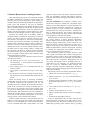
shown in Table 1 as an abstract example. An object oi has
attribute aj if row i and column j is marked with an ✕ in
Table 1 (the example stems from Lindig and Snelting
[10]). For this table, also known as relation table, the following equations hold:
σ ( { o 1 } ) = { a 1, a 2 }
τ ( { a 7, a 8 } ) = { o 3, o 4 }
a3
a4
a5
o2
✕
✕
✕
o3
✕
✕
o4
✕
✕
o1
a1
a2
✕
✕
✕
a6
a7
a8
✕
✕
✕
✕
✕
✕
Table 1: Example relation.
A pair (O, A) is called concept if A = σ ( O ) ∧ O = τ ( A )
holds, i.e., all objects share all attributes. For a concept c =
(O, A), O is the extent of c, denoted by extent(c), and A is
the intent of c, denoted by intent(c).
Informally, a concept corresponds to a maximal rectangle of filled table cells modulo row and column permutations. For example, Table 2 contains the concepts for the
relation in Table 1.
C1
({o1, o2, o3, o4}, ∅)
C2
({o2, o3, o4}, {a3, a4})
C3
({o1}, {a1, a2})
C4
({o2, o4}, {a3, a4, a5})
C5
({o3, o4}, {a3, a4, a6, a7, a8})
C6
({o4}, {a3, a4, a5, a6, a7, a8})
C7
(∅, {a1, a2, a3, a4, a5, a6, a7, a8})
Table 2: Concepts for Table 1.
The set of all concepts of a given formal context forms
a partial order via:
( O 1, A 1 ) ≤ ( O 2, A 2 ) ⇔ O 1 ⊆ O 2 or equivalently with
( O 1, A 1 ) ≤ ( O 2, A 2 ) ⇔ A 1 ⊇ A 2 .
If c1 ≤ c2 holds, then c1 is called a subconcept of c2
and c2 is called superconcept of c1. For instance,
({o2, o4}, {a3, a4, a5}) ≤ ({o2, o3, o4}, {a3, a4}) is true in
Table 2.
The set L of all concepts of a given formal context and
the partial order ≤ form a complete lattice, called concept
lattice:
O
L(C) = { ( O, A ) ∈ 2 × 2
A
A = σ(O) ∧ O = τ( A)}
The infimum of two concepts in this lattice is computed by intersecting their extents as follows:
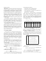
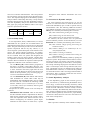
shown in Figure 2. The content of a node N in this representation can be derived as follows:
• the objects of N are all objects at and below N,
• the attributes of N are all attributes at and above N.
For instance, the node in Figure 2 marked with o2 and
a5 is the concept ({o2, o4}, {a3, a4, a5}).
( O 1, A 1 ) ∧ ( O 2, A 2 ) = ( O 1 ∩ O 2, σ ( O 1 ∩ O 2 ) )
The infimum describes a set of common attributes of
two sets of objects. Similarly, the supremum is determined by intersecting the intents:
a3, a4
a1, a2
o1
a5
o2
( O 1, A 1 ) ∨ ( O 2, A 2 ) = ( τ( A 1 ∩ A 2), A 1 ∩ A 2 )
The supremum ascertains the set of common objects,
which share all attributes in the intersection of two sets of
attributes.
C1
<
C6
4.1. Context for Scenarios and Subprograms
C7
Figure 1. Concept lattice for Table 1.
The concept lattice for the example relation in Table 1
can be graphically depicted as a directed acyclic graph
whose nodes represent concepts and whose edges denote
the superconcept/subconcept relation < as shown in
Figure 1. The most general concept is called the top element and is denoted by . The most special concept is
called the bottom element and is denoted by ⊥ .
The combination of the graphical representation in
Figure 1 and the contents of the concepts in Table 2 form
the concept lattice. The complete information can be visualized in a more readable equivalent way by marking only
the graph node with an attribute a ∈ A whose represented
concept is the most general concept that has a in its intent.
Analogously, a node will be marked with an object o ∈ O
if it represents the most special concept that has o in its
extent. The unique element µ in the concept lattice marked
with a is therefore:
∨ { c ∈ L(C ) a ∈ intent ( c ) }
EQ (1)
∧ { c ∈ L(C ) o ∈ extent ( c ) }
EQ (2)
The unique element γ marked with object o is:
γ (o) =
Figure 2. Sparse representation of Figure 1.
In order to derive the feature-component map via concept analysis, one has to define the formal context
(objects, attributes, relation) and to interpret the resulting
concept lattice accordingly.
concept
C5
C4
µ(a) =
o4
4. Dynamic Analysis
C2
C3
a6, a7, a8
o3
We will call a graph representing a concept lattice
using this marking strategy a sparse representation of the
lattice. The equivalent sparse representation for Figure 1 is
The goal of the dynamic analysis is to find out which
subprograms contribute to a given set of features. For each
feature, a scenario is prepared that exploits this feature.
Hence, subprograms will be considered objects of the formal context, whereas scenarios will be considered
attributes. In the reverse case, the concept lattice is simply
inverted but the derived information will be the same.
The relation for the formal context necessary for concept analysis is thus defined as follows:
(s, S) ∈ R if and only if subprogram s is required
for scenario S; a subprogram is required when it
needs to be executed.
In order to obtain the relation, a set of scenarios needs
to be prepared where each scenario executes preferably
only one relevant feature. Then the system is used according to the set of scenarios, one at a time, and the execution
summaries are recorded. Each system run yields all
required subprograms for a single scenario, i.e., one column of the relation table can be filled per system run.
Applying all scenarios provides the complete relation
table.
4.2. On Features and Scenarios
Because one feature can be invoked by many scenarios
and one scenario can invoke several features, there is not
always a strict correspondence between features and scenarios. If there is an n:m mapping between scenarios and
features, one has to locate the concepts in the lattice where
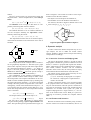
scenarios contributing to a feature overlap. Assume we
analyze a drawing tool and features are the ability to draw
different types of objects, like circles, rectangle, etc., and
the ability to apply different actions on drawn objects, like
move, rotate, or scale. Let us further assume that we have
four scenarios: scenario SA is “draw a circle and move it”,
SB is “draw a circle and scale it”, SC is “draw a rectangle
and move it”, and SD is “draw a rectangle and scale it”. In
the concept lattice for these scenarios, the concept including SA and SC will include all subprograms related to the
feature move whereas the concept including SB and SD
contains the subprograms for the scaling feature. The concept including SA and SB includes all subprograms needed
to draw circles, the concept including SC and SD includes
all subprograms related to rectangles. Because features are
combined in scenarios, one has to interpret the results
revealed by the concept lattice. For instance, if the system
is implemented in an object-oriented style in which the
actions on each object type are implemented by a separate
subprogram, one will get concepts each including one
object type and one action. Presumably, there are some
subprograms needed for all operations on circles (like
drawing and hiding), which will go into one subconcept
(see Figure 3).
from the concept lattice. Consequently, we will assume
that a scenario can easily be mapped onto a feature in the
following.
4.3. Interpretation of the Concept Lattice
Figure 3. Concept lattice A.
Concept analysis applied to the formal context
described in the last section yields a lattice, from which
interesting relationships can be derived. These relationships can be fully automatically derived and presented to
the analyst such that the theoretical background can be
hidden. The only thing an analyst has to know is how to
interpret the derived relationships. This section explains
how interesting relationships can be derived automatically.
As already abstractly described in Section 3 the following base relationships can be derived from the sparse representation of the lattice (note the duality):
• A subprogram s is required for all scenarios at and
above γ(s) – as defined by EQ(1) on page 4 – in the lattice.
• A scenario S requires all subprograms at and below
µ(S) – as defined by EQ(2) on page 4 – in the lattice.
• A subprogram s is specific to exactly one scenario S if
S is the only scenario on all paths from γ(s) to the top
element.
• A scenario S is specific to exactly one subprogram s if s
is the only subprogram on all paths from µ(S) to the
bottom element (i.e, s is the only subprogram required
to implement scenario S).
• Scenarios to which two subprograms s1 and s2 jointly
contribute can be identified by γ(s1) ∨ γ(s2). In the lattice, it is the closest common node toward the top element starting at the nodes to which s1 and s2 are
attached. All scenarios at and above this common node
are those jointly implemented by s1 and s2.
In an alternative functional-style implementation, in
which each subprogram implements actions on different
types of objects, one will get one concept for each action
including scenarios for all object types (see Figure 4).
Interestingly enough, the concept lattice will thus show
whether an object-oriented or functional-style implementation was chosen.
• Subprograms jointly required for two scenarios S1 and
S2 are described by µ(S1) ∧ µ(S2). In the lattice, it is the
closest common node toward the bottom element starting at the nodes to which S1 and S2 are attached. All
subprograms at and below this common node are those
jointly required for S1 and S2.
circlescale
circlemove
circlealign
circlescale
circlemove
circlealign
circledraw
circlemove
rectmove
linemove
circlerotate
rectrotate
linerotate
Key:
scenario1
scenario2
...
circlealign
rectalign
linealign
Figure 4. Alternative concept lattice B.
In most cases the relationship between scenarios and
features is a 1:1 mapping or is at least intuitively clear
• Subprograms required for all scenarios can be found at
the bottom element.
• Scenarios that require all subprograms can be found at
the top element.
Beyond these relationships between subprograms and
scenarios, further useful aspects between scenarios on one
hand and between subprograms on the other hand may be
derived:
• If γ(s1) < γ(s2) holds for two subprograms s1 and s2,
then subprogram s2 is more specific with respect to the
given use case than subprogram s1 because s1 contributes not just to the features for which s2 contributes,
but also to other features.
• If µ(S1) < µ(S2) holds for two scenarios S1 and S2, then
scenario S2 is based on scenario S1 because if S2 is executed, all subprograms in the extent of µ(S1) need also
to be executed.
Thus the lattice also reflects the level of application
specificity. The information described above can be
derived by a tool and fed back to the analyst. Inspecting
the relationships derived from the concept lattice, a decision may be made to analyze only a subset of the original
features in depth due to the additional dependencies that
concept analysis could reveal. All subprograms required
for these features (easily derived from the concept lattice)
form a starting point for further static analyses to identify
components, to investigate quality (like maintainability,
extractability, and integrability) and to estimate effort for
subsequent steps.
5. Static Dependency Analysis
From the concept lattice, we can easily derive all subprograms executed for any set of relevant features (note
that we use features and scenarios as synonyms from here
on, see Section 4.2). However, this gives us only a set of
subprograms, but it is not clear which of these subprograms form a feature-specific component and which of
them are general-purpose subprograms that are only used
as building blocks for other components but do not contain
any feature-specific logic. Given a feature f of interest this
question can be answered as follows:
• As a first approximation, all subprograms in the extent
of concept µ(f) according to EQ(2) on page 4 may
jointly constitute a component.
• Irrelevant subprograms among these subprograms can
be sorted out by a goal-directed manual inspection.
5.1. Building the Starting Set
All subprograms in the extent of a concept jointly contribute to all features in the intent of the concept, which
immediately follows from the definition of a concept.
However, there may also be subprograms in the extent that
contribute to other features as well, so they are not specific
to the given feature. There may be subprograms in the
extent that do not contain any feature-specific code at all.
Thus, subprograms in the extent of the concept need to be
inspected manually. Because there are no reliable criteria
known that distinguish feature-specific code from generalpurpose code, this analysis cannot be automated and
human expertise is necessary. However, the concept lattice
may narrow the candidates for manual inspection.
The concept lattice and the dependency graph can help
to decide in which order the subprograms are to be
inspected such that the effort for manual inspection can be
reduced to a minimum. Since we are interested in subprograms most specific to a feature f we start at those subprograms s that are attached to µ(f), i.e., for which µ(f) = γ(s)
holds. If there are no such subprograms, we collect all
concepts below µ(f) with minimal distance from µ(f) to
which subprograms are attached. There can be more than
one concept, so we unite all subprograms that are attached
to one of these concepts. The subset of subprograms identified in this step and accepted by manual inspection is
called the starting set S(f).
5.2. Inspection of the Static Call Graph
Next, we inspect all subprograms called from subprograms in S(f). We generate the call graph (as one specific
subset of the dependency graph) that contains all subprograms transitively called by subprograms in S(f) as derived
by a static analysis. We concentrate on subprograms here
because they are the active constituents of a component.
Global variables and types may be added once all subprograms have been identified. Subprograms in S(f) are said
to be the roots of this call graph. A static points-to analysis
is needed to resolve calls via function pointers if present.
The static points-to analysis may take advantage of the
knowledge about actually called functions yielded by the
dynamic analysis.
It is sufficient to consider only those subprograms s for
which s ∈ extent (µ(f)) holds because only those subprograms are actually called when f is invoked according to
the dynamic analysis. Hence, we combine static and
dynamic information to eliminate conditional static subprogram calls in order to reduce the search space.
If the component for the feature f is to be understood,
calls to subprograms not in extent(µ(f)) can be safely
ignored in the original source code in order to cut apparent
static dependencies – unless there is another relevant feature relying on the same subprogram and in whose context
the call is actually executed. In this case, one can apply
slicing techniques to separate the code relevant for each
feature.
Once the call graph is generated, it can be traversed to
inspect subprograms. Any kind of traversal is possible, but
a depth-first search is most suited because a subprogram
can only be understood if all its called subprograms are
understood. Moreover, in a breadth-first search, a human
has to cope with continuous context switches. The goal of
the inspection is to sort out subprograms that do not
belong to the component in a narrow sense because they
do not contain feature-specific code. Two additional analyses gather further information useful while navigating on
the call graph:
• Strongly connected component analysis is used to identify cycles in the call graph: If there is one subprogram
in a cycle that contains feature-specific code, all subprograms of the cycle need to be added to the component because of the cyclic dependency.
• Dominance analysis is used to identify subprograms
that are local to other subprograms. A subprogram s1 is
said to dominate another subprogram s2 if every path in
the call graph from one of its roots in S(f) to s2 contains
s1. In other words, s2 can only be called by way of s1. If
a subprogram s is found to be feature-specific, then all
its dominators also need to be added to the component,
because they need to be called in order for s to be executed. If neither of a dominator’s dominatees contain
feature-specific code and the dominator itself is not
feature-specific, then the dominator is a clear cutting
point as all its dominatees are local to it. Consequently,
the dominator and all its dominatees can be safely
omitted while understanding the system.
Inspection is done along the call relation in the call
graph rather than following a top-down traversal in the
concept lattice because the lattice does not really reflect
the dependencies: γ(s1) > γ(s2) does not imply that s1 calls
s2. However, the concept lattice may still provide useful
information for the inspection. In Section 4.3 we made the
observation that the lower a concept γ(s) is in the lattice,
the more general subprogram s is as it serves more features – and vice versa. Thus, the concept lattice gives us
insight into the level of abstraction of a subprogram and,
therefore, contributes to the degree of confidence that a
specific subprogram contains feature-specific code.
If more than one feature is relevant, one simply unites
the starting sets for each feature and then follows the same
approach. For more than one feature, the concept lattice
provides insight into feature interaction and identifies subprograms jointly used by several features. Such subprograms can then be considered a component of their own.
Hence, not only one component is detected but the call
graph is partitioned into several connected components by
merging connected concepts in the lattice and by filtering
out subprograms in their extent.
Once all subprograms have been identified, static
dependency analysis, e.g., program slicing, can be used to
extract the components’ code including necessary variable
and type declarations. Moreover, static dependency analysis will also be used to identify the provided interface of
the extracted components – those elements of a component used in other parts of the system – and the required
interface – those elements of the system the component’s
elements rely on and that are not declared by the component itself.
6. Implementation
The implementation of detecting the executed subprograms per scenario and applying concept analysis is surprisingly simple (if one already has a tool for concept
analysis). Our prototype for a Unix environment is an
opportunistic integration of the following parts:
• Gnu C compiler gcc to compile the system using a
command line switch for generating profiling information,
• Gnu object code viewer nm and a short Perl script in
order to identify all functions of the system (as
opposed to those included from standard libraries),
• Gnu profiler gprof and a short Perl script to ascertain
the executed functions in the execution summary,
• concept analysis tool concepts [11],
• graph editor Graphlet [2] to visualize the concept lattice,
• one short Perl script to convert the file formats of concepts and Graphlet (147 LOC),
• and our extended version of Rigi [22].
For deriving the static dependency graph and to identify components, we have developed the Bauhaus toolkit
[1]. It allows deriving detailed dependencies as system
dependency graph (SDG) [9] and more coarse-grained
dependencies as resource flow graph (RFG) [12]. An SDG
describes set-use data dependencies and control dependencies at the level of expressions and statements, while an
RFG contains only global declarations (global variables,
user-defined types, and subprograms) and their relationships (variable access, signature relations, calls, etc.). The
RFG is derived from the SDG by abstracting from individual expressions and statements and is better suited for presentation to a human analyst. The Bauhaus toolkit uses
Rigi [22] to visualize the RFG. Rigi supports graph navigation and provides immediate access to the original
source code for a more detailed investigation. We added
multiple additional automatic analyses specifically to support component retrieval [13], like identification of cyclic
dependencies and local (i.e., dominated) parts (see Section
5.2).
7. Case Study
We analyzed two web browsers (see Table 3) using the
same set of relevant related features. The concept lattice
for each of these systems was derived as described in Section 6. The required subprograms as identified by dynamic
analysis and the relationships derived by concept analysis
formed a starting point for the static dependency analysis.
The static dependency analysis was done on the resource
flow graph [12] using the Bauhaus toolkit. The experiences are reported in this section.
System
Version
KLOC (wc)
#subprograms
Mosaic
2.6
51,440
701
Chimera
2.0a19
38,208
928
Table 3: Analyzed web browsers.
7.1. Case Study Setup
In two experiments, History and Bookmark, we tried to
understand how two specific sets of related features are
implemented in both browsers using the process described
above. The goal of this analysis was to recover the featurespecific components and the way they interact, i.e., to
reverse engineer a partial description of the software architecture. The partial software architecture, for instance,
allows one to decide whether feature-specific components
can be extracted from one system and integrated into
another system with only minor changes. Chimera does
not implement all features that Mosaic provides and we
wanted to find out whether the respective feature-specific
components of Mosaic can be reused for Chimera.
Use case History (H): Chimera allows going back in
the history of already visited URLs. However, Chimera does not have a forward button that allows a user
to move forward in the history again after the back
button was used. Mosaic has both a back and forward
button. In this experiment, going back and going forward were considered related features.
Use case Bookmark (B): Both Mosaic and Chimera
offer bookmarks for visited URLs. URLs may be
bookmarked, and bookmarked URLs may be loaded
and removed. We considered the following related
features: addition of a new bookmark for a currently
viewed URL, removal of a bookmark, and navigation
to a bookmarked URL.
The question we want to answer in our case study was
as follows:
Identification and extraction: How are the history
and the bookmark features implemented in Mosaic?
What are the interfaces between the specific components that implement these features and the rest of
Mosaic? Analogously for Chimera’s partial implementation of these features. In both cases, a partial
description of the software architecture was recovered.
7.2. Scenarios for Dynamic Analysis
For each experiment and each browser, we ran the
browser in a start-end scenario in which the browser was
started and immediately quit in order to separate start-up
and shutdown code. The following additional scenarios
were defined specifically to the two experiments. Use case
History was covered by the following three scenarios:
(H1) basic scenario doing nothing but browsing,
(H2) scenario using the back button, and
(H3) scenario using the back and forward buttons.
For Chimera, the last scenario was not performed
(because Chimera possesses no forward button). Use case
Bookmark was covered by the following four scenarios:
(B1) basic scenario: simply opening and closing the
bookmark window,
(B2) scenario: adding a new bookmark for the currently displayed URL,
(B3) scenario: removing a bookmark,
(B4) scenario: selecting a bookmark and visiting the
associated URL.
Each scenario was immediately ended by quitting the
respective system. We provided scenarios that use one feature only except for one scenario: One cannot use the forward button without using the back button. Consequently,
the concept containing subprograms executed for scenario
(H2) is a subconcept of the concept related to (H3). Likewise, a bookmark can only be deleted when an URL has
been added before. However, to circumvent this problem,
we started the browser with a non-empty bookmark file in
all scenarios. Thus, we did not consider the case of insertion into an empty bookmark list.
7.3. Static Dependency Analysis
In the dependency graph for the browsers (given as
RFG, see Section 6), visualized using the Bauhaus extension to Rigi, we derived all statically transitively called
functions (using Rigi’s basic selection facilities) and intersected the static information with the actually executed
functions manually. We additionally filtered out all functions specific to HTML and the X-window-based graphical user interface guided by the browser’s proper naming
conventions. These functions were all in the bottom element of the concept lattice.
7.4. Results
Table 4 provides a summary of the numbers of subpro-
grams that needed to be further considered in each step
and shows how the search space could be reduced in each
step. (H) denotes the history, (B) the bookmark experiment. The total number of all functions of the kernels (not
including libraries such as html, jpeg, zlib) are in column
(1), the number of actually executed subprograms for each
scenario is shown in column (2). All functions statically
called by subprograms selected from the set of dynamically executed functions in upper concepts of the lattice
are in column (3). The intersection of column (2) and (3)
is contained in column (2) ∩ (3). Column relevant reports
all functions in column (2) ∩ (3) that are specific to the
selected features according to our manual inspection. All
other functions are used for other purposes than bookmarks and histories.
(1)
Mosaic/(B)
(2)
701
Mosaic/(H)
Chimera/(B)
928
Chimera/(H)
(2) ∩ (3)
(3)
relevant
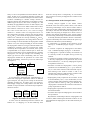
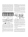
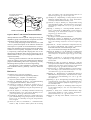
Results for History. The interface between Mosaic’s
browser kernel and the history component (see Figure 6) is
formed by three subprograms to (a) get the current URL,
(b) set the current URL, and (c) communicate the action
and event (changed URL).
The history component can be easily extracted from
Mosaic’s source code because it is a separate component –
while the history is an integral part of Chimera’s kernel.
There is no set of subprograms of Chimera that could be
reasonably addressed as “history manager component” as
in Mosaic. Chimera uses a layer of wrappers calling a dispatching routine around a list of actions where the displayed URLs are part of that list.
As the analysis of the partial architectural architectures
reveals, re-using Mosaic’s history components in Chimera
would be very difficult due to the architectural mismatch
[7].
359
99
74
16
348
74
65
6
the meaning of the letters is
described in the text
431
89
55
3
history
419
123
55
24
Table 4: Subprogram counts for Mosaic and Chimera
GUI
dispatch
(b)
(a)
browser
navigate
remove
GUI
(c)
inner
state
add
upper region
Mosaic’s history
component
browser
here, the
history is
located
Chimera’s history
data storage
procedure call
Figure 6. Mosaic’s and Chimera’s history architecture
lower region
procedure calls procedure
Figure 5. Relevant parts of Chimera for history
Eventually, only a small number of subprograms
needed to be inspected more thoroughly due to the topdown inspection process. As an example, Figure 5 shows
the remaining subprograms of Chimera (omitting their
names) relevant to the history experiment. This picture
clearly shows the possible cutting points in the dependency graph between functions specific to the history features (upper region) and non-specific functions (lower
region).
We recovered the parts of the architecture of Mosaic
and Chimera relevant to the two use cases. The recovered
partial architecture shows that Chimera’s browser kernel is
built around a list of visited URLs whereas Mosaic’s
browser kernel does not know the history of visited URLs
at all.
Results for Bookmarks. The partial architectures of the
two systems are similar to each other with respect to bookmarks. Both architectures include an encapsulated bookmark component, which communicates via a narrow
interface with the basic browser kernel (see Figure 7).
The basic actions that have to be performed are: (a) get
currently shown URL, (b) set currently shown URL, (c)
display the bookmarks, and (d) communicate the bookmark selection back.
Exchanging the two implementations between Mosaic
and Chimera would be reasonably easy.
8. Conclusions
The technique presented in this paper identifies all
components specific to a set of related features using execution traces for different usage scenarios. At first, concept
analysis – a mathematically sound technique to analyze
binary relations – allows to locate the most feature-specific
subprograms among all executed subprograms. Then, a
static analysis uses these feature-specific subprograms to
the meaning of the letters is
described in the text
book-
(c)
(d)
(b)
GUI
(a)
book- (c)
marks
(d)
(b)
(a)
browser
browser
Mosaic’s bookmarks
parts‘, Proceedings of the 17th International Conference on
Software Engineering, pp. 179-185, April 1995
GUI
dispatch
inner
state
Chimera’s bookmarks
Figure 7. Mosaic’s and Chimera’s bookmark architecture
identify additional feature-specific subprograms along the
dependency graph. The combination of dynamic and static
information reduces the search space drastically.
In a case study, analyzing two web browsers, we could
recover a partial description of the software architecture
with respect to a specific set of related features. Commonalities and variabilities between these partial architectures
could be recovered quickly. Altogether, we found 16 and
6, respectively, feature-specific subprograms out of 701
subprograms for Mosaic and 3 and 24, respectively, out of
928 for Chimera. Only very few subprograms needed to be
inspected manually.
Deriving partial architectures with the described technique can support a more goal-oriented and cost-effective
program understanding and reverse engineering, thereby
facilitating feature-specific re-use and reengineering.
The approach is only applicable to externally visible
and executable features, primarily suited for functional
features.
References
[1] Bauhaus project, University of Stuttgart,
http://www.informatik.uni-stuttgart.de/ifi/ps/bauhaus.
[2] Brandenburg, F.J., ‘Graphlet’, Universität Passau,
http://www.infosun.fmi.uni-passau.de/Graphlet.
[3] Booch, G., Rumbaugh, Jacobson, J., ‘The Unified Modeling
Language Reference Manual’, Addison-Wesley.
[4] Canfora, G., Cimitile, A., De Lucia, A., Di Lucca, G.A., ‘A
Case Study of Applying an Eclectic Approach to Identify
Objects in Code’, Workshop on Program Comprehension, pp.
136-143, 1999.
[8] Graudejus, H., ‘Implementing a Concept Analysis Tool for
Identifying Abstract Data Types in C Code’, master thesis,
University of Kaiserslautern, Germany, 1998.
[9] Horwitz, S., Reps, T., Binkley, D., ‘Interprocedural slicing
using dependence graphs’, ACM Transactions on Programming Languages and Systems, vol. 12, no. 1, pp. 26-60, January 1990.
[10]Lindig, C., Snelting, G., ‘Assessing Modular Structure of
Legacy Code Based on Mathematical Concept Analysis’,
Proceedings of the International Conference on Software
Engineering, pp. 349-359, 1997.
[11]Lindig, C., Concepts,
ftp://ftp.ips.cs.tu-bs.de/pub/local/softech/misc.
[12]Koschke, R., Girard, J.-F., Würthner, M., ‘An Intermediate
Representation for Reverse Engineering Analyses’, Proceedings of the Working Conference on Reverse Engineering,
1998.
[13]Koschke, R., ‘Atomic Architectural Component Recovery
for Program Understanding and Evolution’, Dissertation,
Institut für Informatik, Universität Stuttgart, 2000,
http://www.informatik.uni-stuttgart.de/ifi/ps/rainer/thesis.
[14]Krone, M., Snelting, G., ‘On the Inference of Configuration
Structures From Source Code’, Proceedings of the International Conference on Software Engineering, pp. 49-57, May
1994.
[15]Kuipers, T., Moonen, L., ‘Types and Concept Analysis for
Legacy Systems’, Proc. Int. Workshop on Program Comprehension, 2001.
[16]Sahraoui, H., Melo. W, Lounis, H., Dumont, F., ‘Applying
Concept Formation Methods to Object Identification in Procedural Code’, Proceedings of the Conference on Automated
Software Engineering, pp. 210-218, November 1997.
[17]Siff, M., Reps, T., ‘Identifying Modules via Concept Analysis’, Proceedings of the International Conference on Software Maintenance, pp. 170-179, October 1997.
[18]Snelting, G., ‘Reengineering of Configurations Based on
Mathematical Concept Analysis’, ACM Transactions on Software Engineering and Methodology vol. 5, no. 2, pp. 146189, April 1997.
[19]Snelting, G., Tip, F., ‘Reengineering Class Hierarchies Using
Concept Analysis’, Proceedings of the ACM SIGSOFT Symposium on the Foundations of Software Engineering, pp. 99110, November 1994.
[20]van Deursen, A., Kuipers, T., ‘Identifying objects using cluster and concept analysis’, Proc. Int. Conf. Software Engineering, 1999.
[5] Chen, K., Rajlich, V., ‘Case Study of Feature Location Using
Dependence Graph’, Proc. of the 8th Int. Workshop on Program Comprehension, pp. 241-249, June 2000.
[21]Wilde, N., Scully, M.C., ‘Software Reconnaissance: Mapping Program Features to Code’, Software Maintenance:
Research and Practice, vol. 7, pp. 49-62, 1995.
[6] Eisenbarth, E., Koschke, R. Simon, D., ‘Feature-Driven Program Understanding Using Concept Analysis of Execution
Traces’, Proc. Int. Workshop on Program Comprehension,
2001, to appear.
[22]Wong, K., ‘The Rigi User’s Manual’, Version 5.4.4., June
1998.
[7] Garlan, D., Allen, R., Ockerbloom, J., ‘Architectural Mismatch or, Why it’s hard to build systems out of existing