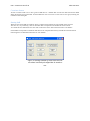
1
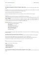
IntR – Interactive GUI for R
Fabio Veronesi
USER MANUAL
Introductory Notes
This software is a simple interface for compiling R script interactively. After the script is compiled it runs it in
batch mode. All the computations are done using packages already present in R and NOT CREATED BY THE
AUTHOR OF THIS SOFTWARE INTERFACE.
The packages with the relative authors are listed below:
- GSTAT: Pebesma, E.J., 2004. Multivariable geostatistics in S: the gstat package. Computers &
Geosciences, 30: 683-691.
- sp: Pebesma, E.J., R.S. Bivand, 2005. Classes and methods for spatial data in R. R News 5 (2),
http://cran.r-project.org/doc/Rnews/. Roger S. Bivand, Edzer J. Pebesma, Virgilio Gomez-Rubio, 2008.
Applied spatial data analysis with R. Springer, NY. http://www.asdar-book.org/
- maptools: Nicholas J. Lewin-Koh and Roger Bivand
- RandomForest: A. Liaw and M. Wiener (2002). Classification and Regression by randomForest. R
News 2(3), 18--22.
- tree: Brian Ripley
- rgdal: Timothy H. Keitt, Roger Bivand, Edzer Pebesma, Barry Rowlingson
- lattice: Sarkar, Deepayan (2008) Lattice: Multivariate Data Visualization with R. Springer, New York.
ISBN 978-0-387-75968-5
- akima: Albrecht Gebhardt (1998). Akima: Interpolation of irregularly spaced data
Note on R
R is a very powerful statistical language. However it is also a slow language and this is clear in geostatistical
interpolations.
For this reason, especially when it is interpolating with inverse distance, it takes some time to finish the process.
Do not worry too much and let it works.
System Requirements
The system requirements are the same of R. In this version of IntR is included the version 2.12.0 of R, that is
used to run the scripts. This version of R is compatible with 32bit machines. On these machines R can run but it
has some memory limitations. It can use a maximum of 4 Gb of RAM (but in some machines the amount is
limited at 2 or 3 Gb of RAM). This means that sometimes R will not be able to complete the process because it
is not able to allocate the data onto the RAM. However, there are some ways to limit the amount of memory
necessary for complete the process. The common tip is to reduce the size of data and covariates. In IntR the user
can choose in every step of the process the resolution of the ascii grid and the resolution of the map that he
wants to create. This way, if the user notices that R does not complete the process because of a memory related
problem, he can just decrease the resolution and try again. The only way to increase the memory that R can use
for its computation is to use a 64bit machine. On these machines the upper limit of RAM that can be used by R
is virtually unlimited.
Data Format
IntR works with data file arrange in a textual table, in txt format. The structure of the file must be like the
following example:
ID
1
2
3
4
Lat
xxxxxx.xx
xxxxxx.xx
xxxxxx.xx
xxxxxx.xx
Lon
yyyyyy.yy
yyyyyy.yy
yyyyyy.yy
yyyyyy.yy
value
ii
iii
iiii
iiii
The format of the two spatial coordinates is not important, because within the sp package in R there is the
possibility to set the projection of your data, according to the proj4string format (http://spatialreference.org/).
Once the user insert the correct projection of his data, all the interpolation will consider the Euclidean distance
between data points. The important thing is that the header of the file is exactly the same of the above example.
IntR – Interactive GUI for R
Fabio Veronesi
Covariates format
All the covariates need to be in ascii grid. In IntR there is a module that converts the data between the ESRI
shape file and the ascii grid format. In this module the user can convert a raster into an ascii grid, selecting the
resolution of the final grid.
Starting IntR
When the user starts IntR, the software shows a window with a button for each module of the program.
The user can, very intuitively, click on the button that corresponds to the module he wants to start.
To consult this user manual the user can click on the menu “File” and on the menu item “User Guide”.
Each module corresponds to a different task that will be compiled interactively in IntR and executed with R.
Following there are detailed instructions for each module.
Figure 1: starting window of IntR. Here the user
can select intuitively the algorithm he needs to
use.
IntR – Interactive GUI for R
Fabio Veronesi
Variogram & Anisotropy
In IntR there are two modules that are used for performing some preliminary studies upon the study area. These
two modules are “Variogram Plot” and “Anisotropy”.
Variogram Plot
Variogram plot studies the spatial variability of the dataset performing the variogram computation. The results
are a series of three images, the omnidirectional variogram, four directional variograms a 0, 45, 90 and 135
degrees and a variogram map that can be used to assess the anisotropy of the field.
Installation
Simply run the script START.exe and select Variogram Plot from the buttons.
In order to run the software all the data and covariates that you need for running the interpolation must be in the
folder c:\RHOME.
Running the Program
The working flow for Variogram Plot is the following:
select data file
input of ID number of the projection
select number and covariates files
input the linear regression model
select the variogram model
execute the cross-validation
This module can be used for an ordinary kriging variogram or for computing a regression variogram, which uses
a linear regression module. Even if the user wants to perform a simple ordinary kriging variogram, he needs to
insert a covariate file that will be used for the variogram boundary.
Results
At the end of the module, IntR displays a window with three buttons that are used to show the images of the
variograms.
Anisotropy
Anisotropy is a module that is used to provide the user with the two values used to assess the geometrical
anisotropy of the field.
A geometrical anisotropy is evident when the directional variograms show the same sill but different ranges. To
correct this anisotropy the user needs to insert two parameters, the angle of the direction of maximum
continuity, in positive degrees from north, and the ratio between the range in the direction of maximum
continuity and the range in the direction of minimum continuity.
Installation
Simply run the script START.exe and select Anisotropy from the buttons.
In order to run the software all the data that you need for running the interpolation must be in the folder
c:\RHOME.
Running the Program
This module asks only for the data file, the projection and an ascii grid for bounding the variograms.
Results
At the end of the module, IntR displays a window with the values of the two parameters used to correct the
geometrical anisotropy. Those 2 values are saved in a txt file called parameters.txt within the RHOME folder.
To correct the anisotropy the user needs to insert manually the two parameters when asked in one of the kriging
modules.
IntR – Interactive GUI for R
Fabio Veronesi
Universal Kriging
This python script will help you compiling and running a script able to perform a Universal kriging on your
data. The kriging is performed with the package Gstat.
Installation
Simply run the script START.exe and select Universal Kriging from the buttons.
In order to run the software all the data and covariates that you need for running the interpolation must be in the
folder c:\RHOME.
All the covariates need to be in ascii grid (*.asc) format. To convert a table with Latitude, Longitude and
covariate value into .asc you can use the Inverse Distance algorithm in IntR or any other GIS software. To
convert an ESRI raster into an ascii grid use the module from SHP to ASC.
Running the Program
The working flow for Universal Kriging is the following:
input of ID number of the projection
select data file
select the prediction-grid size
select number and covariates files
input the linear regression model
select the variogram model
execute the cross-validation
perform the kriging
The first information the program needs is the ID number of the projection. For more information see paragraph
"Projection" below.
After that, the program will ask you to choose the data file.
The data file can be a txt and the format has to be the same of the one presented in the Data Format paragraph.
In the next input windows IntR asks you to insert the grid size of your prediction grid.
If you insert 10, for example, it means that IntR will predict a value on a square grid of dimension 10x10 m.
Subsequently, the program will ask for the covariate number and to select the covariates files.
Be careful during this step because if you need to insert 2 covariates, for example, the second file selection
window, for selecting the second covariate, will appear very shortly after the first.
At this point you must insert the linear regression model. The model has to be in the form:
covariate1+covariate2+......+covariateN
Ex.
if the two covariates are named slope.asc and em38h.asc
the model will be:
slope.asc+em38h.asc
it is important to insert the entire name of the file, extension included.
When you finish input the linear regression model, IntR asks you for some variogram parameters, such as the
variogram model and the fitting algorithm. It important to insert the name as it is shown on the screen.
Ex.
on the screen you will see a message like,
"Please write the model of the variogram.
Type:
- 0 for the default model,
- Sph for Spherical Model,
- Exp for Exponential model,
- Gau for Gaussian model
- Mat for the Matern. "
IntR – Interactive GUI for R
Fabio Veronesi
if you want the spherical model, you need to insert Sph, with the first letter in capital.
For the fitting, if you want the reml, just type reml (no capitals), or gls (no capitals) for the generalized least
square.
Subsequently a dialog appears and asks for the two anisotropy parameter. The user, if an anisotropy is presents,
needs to insert the two numbers separated by a comma. If no anisotropy is present in the field, the user needs to
insert a single 0.
Ex.
Parameter p is 45 and the parameter s is 0.5.
The user has to insert: 45,0.5
At this point, the cross-validation starts.
After it finishes the cross-validation, it shows a window with the R Squared value of it and a button that shows
the variogram image, which is also saved on “C:\”.
If the result of the cross-validation is satisfying, you can click on "YES" and automatically proceed with the
kriging with the same linear regression model.
If the result is not good you can click on "NO" and repeat the cross-validation selecting again the linear
regression model and all the parameters of the variogram.
Projection
To set the projection of the map you need to insert the ID number of the coordinates system. You can find a list
of ID number and the relative system here:
http://spatialreference.org/ref/?search=utm&srtext=Search
At the moment, IntR supports only EPSG projections, so you need to insert a number of an EPSG projection.
If your data are unprojected insert 0 in the apposite space.
It is important to insert the projection ID, if the data are projected, because the package GSTAT has been
designed to work with projections. This means that if the projection is available, the interpolation is done using
Euclidean Distances.
Output
The output of the script are:
- variogram plot in jpg
- prediction map in jpg
- kriging error map in jpg
- cross-validation of the last used model in txt
- kriging results table in txt
- ascii grid of the map
- shp file with predicted points
IntR – Interactive GUI for R
Fabio Veronesi
Inverse Distance
This program performs an inverse distance interpolation.
The data file can be a txt and the format has to be the same of the one presented in the Data Format paragraph.
However, this module asks for the name of the variable of interest, so the user can use a file with different
variables and perform an IDW (inverse distance weighted) for each variable of interest.
Running the Program
The working flow for Inverse Distance is the following:
select data file
input of ID number of the projection
select the prediction-grid size
select the ascii grid file
select the inverse distance power
select the percentage of data excluded for validation
execute the cross-validation
perform the inverse distance
The inverse distance algorithm asks first for a data file. Then it asks for a projection ID number (see paragraph
"Projection" in the Universal kriging section). If the file is unprojected, or if you don't want to consider
projection in your computation, type 0.
After that, IntR asks you to select an Ascii Grid that will be used as a base for the final interpolation. The asc
file can be the result of the script SHPtoASC.
The next step requires you to select the power of the inverse distance, the default is 2.
Then you need to select the percentage of samples to exclude for validation. In this case, the validation is done
creating two subsets of the data a training and a test subset based on the percentage of samples that the user
inserted. Then it interpolates the training data and predicts the variable in the test locations. In the end it
compares the observed and predicted values, giving the R Square and the plotting the results.
The final step is to proceed with the inverse distance, which uses all the available data, and plots a Prediction
Map in jpeg.
Results
After the validation, IntR shows a window with the R squared of the validation and a button to show a plot of
the results. The plot shows the observed versus the predicted values, with a red line on the 45 degrees line and a
black line that correspond to the linear regression between observed and predicted.
At the end of the module, it shows the map with the prediction of the interpolation.
IntR – Interactive GUI for R
Fabio Veronesi
Regression Kriging
The Regression kriging is an alternative to Universal kriging. The difference is that the linear regression is done
separately from the variogram computation.
The script is very similar to Universal Kriging.
Installation
Simply run the script START.exe and select Regression Kriging from the buttons.
In order to run the software all the data and covariates that you need for running the interpolation must be in the
folder c:\RHOME.
All the covariates need to be in ascii grid (*.asc) format. To convert a table with Latitude, Longitude and
covariate value into .asc you can use the Inverse Distance algorithm in IntR or any other GIS software. To
convert an ESRI raster into an ascii grid use the module from SHP to ASC.
Running the Program
The working flow for Regression Kriging is the following:
input of ID number of the projection
select data file
select the prediction-grid size
select number and covariates files
input the linear regression model
select the variogram model
execute the cross-validation
perform the kriging
The first information the program needs is the ID number of the projection. For more information see paragraph
"Projection" below.
After that, the program will ask you to choose the data file.
The data file can be a txt and the format has to be the same of the one presented in the Data Format paragraph.
In the next input windows IntR asks you to insert the grid size of your prediction grid.
If you insert 10, for example, it means that IntR will predict a value on a square grid of dimension 10x10 m.
Subsequently, the program will ask for the covariate number and to select the covariates files.
Be careful during this step because if you need to insert 2 covariates, for example, the second file selection
window, for selecting the second covariate, will appear very shortly after the first.
At this point you must insert the linear regression model. The model has to be in the form:
covariate1+covariate2+......+covariateN
Ex.
if the two covariates are named slope.asc and em38h.asc the model will be:
slope.asc+em38h.asc
it is important to insert the entire name of the file, extension included.
When you finish input the linear regression model, IntR asks you for some variogram parameters, such as the
variogram model and the fitting algorithm. It important to insert the name as it is shown on the screen.
Ex.
on the screen you will see a message like,
"Please write the model of the variogram.
Type:
- 0 for the default model,
- Sph for Spherical Model,
- Exp for Exponential model,
IntR – Interactive GUI for R
Fabio Veronesi
- Gau for Gaussian model
- Mat for the Matern. "
if you want the spherical model, you need to insert Sph, with the first letter in capital.
For the fitting, if you want the reml, just type reml (no capitals), or gls (no capitals) for the generalized least
square.
Subsequently a dialog appears and asks for the two anisotropy parameter. The user, if anisotropy is presents,
needs to insert the two numbers separated by a comma. If no anisotropy is present in the field, the user needs to
insert a single 0.
Ex.
Parameter p is 45 and the parameter s is 0.5.
The user has to insert: 45,0.5
At this point, the cross-validation starts.
After it finishes the cross-validation, it shows a window with the R Squared value of it and a button that shows
the variogram image, which is also saved on “C:\”.
If the result of the cross-validation is satisfying, you can click on "YES" and automatically proceed with the
kriging with the same linear regression model.
If the result is not good you can click on "NO" and repeat the cross-validation selecting again the linear
regression model and all the parameters of the variogram.
Projection
To set the projection of the map you need to insert the ID number of the coordinates system. You can find a list
of ID number and the relative system here:
http://spatialreference.org/ref/?search=utm&srtext=Search
At the moment, IntR supports only EPSG projections, so you need to insert a number of an EPSG projection.
If your data are unprojected insert 0 in the apposite space.
It is important to insert the projection ID, if the data are projected, because the package GSTAT has been
designed to work with projections. This means that if the projection is available, the interpolation is done using
Euclidean Distances.
Output
The output of the script are:
- variogram plot in jpg
- prediction map in jpg
- kriging error map in jpg
- cross-validation of the last used model in txt
- kriging results table in txt
- ascii grid of the map
- shp file with predicted points
IntR – Interactive GUI for R
Fabio Veronesi
Ordinary Kriging
The Ordinary kriging script is similar to the other two kriging script.
The format of the data file is the same, coordinates columns called Lat and Lon and the data column called
value.
The difference of course is that with the ordinary kriging you don't need to insert covariates. However you still
need to insert an ascii grid for interpolating the final prediction map.
The ascii grid can be the result of the SHPtoASC script.
The series of information needed by the software are similar to the one needed for universal kriging.
Installation
Simply run the script START.exe and select Ordinary Kriging from the buttons.
In order to run the software all the data and covariates that you need for running the interpolation must be in the
folder c:\RHOME.
All the covariates need to be in ascii grid (*.asc) format. To convert a table with Latitude, Longitude and
covariate value into .asc you can use the Inverse Distance algorithm in IntR or any other GIS software. To
convert an ESRI raster into an ascii grid use the module from SHP to ASC.
Running the Program
The working flow for Universal Kriging is the following:
input of ID number of the projection
select data file
select the prediction-grid size
select number and covariates files
input the linear regression model
select the variogram model
execute the cross-validation
perform the kriging
The first information the program needs is the ID number of the projection. For more information see paragraph
"Projection" below.
After that, the program will ask you to choose the data file.
The data file can be a txt and the format has to be the same of the one presented in the Data Format paragraph.
In the next input windows IntR asks you to insert the grid size of your prediction grid.
If you insert 10, for example, it means that IntR will predict a value on a square grid of dimension 10x10 m.
Subsequently, the program will ask for an ascii grid. This will be used to bind the variogram.
Ex.
on the screen you will see a message like the following:
"Please write the model of the variogram.
Type:
- 0 for the default model,
- Sph for Spherical Model,
- Exp for Exponential model,
- Gau for Gaussian model
- Mat for the Matern. "
if you want the spherical model, you need to insert Sph, with the first letter in capital.
For the fitting, if you want the reml, just type reml (no capitals), or gls (no capitals) for the generalized least
square.
IntR – Interactive GUI for R
Fabio Veronesi
Subsequently a dialog appears and asks for the two anisotropy parameter. The user, if an anisotropy is presents,
needs to insert the two numbers separated by a comma. If no anisotropy is present in the field, the user needs to
insert a single 0.
Ex.
Parameter p is 45 and the parameter s is 0.5.
The user has to insert: 45,0.5
At this point, the cross-validation starts.
After it finishes the cross-validation, it shows a window with the R Squared value of it and a button that shows
the variogram image, which is also saved on “C:\”.
If the result of the cross-validation is satisfying, you can click on "YES" and automatically proceed with the
kriging with the same linear regression model.
If the result is not good you can click on "NO" and repeat the cross-validation selecting again the linear
regression model and all the parameters of the variogram.
Projection
To set the projection of the map you need to insert the ID number of the coordinates system. You can find a list
of ID number and the relative system here:
http://spatialreference.org/ref/?search=utm&srtext=Search
At the moment, IntR supports only EPSG projections, so you need to insert a number of an EPSG projection.
If your data are unprojected insert 0 in the apposite space.
It is important to insert the projection ID, if the data are projected, because the package GSTAT has been
designed to work with projections. This means that if the projection is available, the interpolation is done using
Euclidean Distances.
Output
The output of the script are:
- variogram plot in jpg
- prediction map in jpg
- kriging error map in jpg
- cross-validation of the last used model in txt
- kriging results table in txt
- ascii grid of the map
- shp file with predicted points
IntR – Interactive GUI for R
Fabio Veronesi
CART
This program performs a CART regression with the package tree.
The data file can be a txt and the format has to be the same of the one presented in the Data Format paragraph,
with the coordinates columns called "Lat" and "Lon" and the variable of interest column called "value", plus an
“ID” column with a single value for every sample. The separation must be a white space.
The first thing to type is the ID number of the projection. Then, like all the other algorithms, CART asks the
user for a data file and for covariates. Then it asks for the size of the prediction grid, for the regression model.
At this point, it starts R runs the script and shows the results, which include a plot of observed versus predicted,
with a red line that indicate the 45 degree line and a black line which is a linear regression between observed
and predicted. Other results are a plot of the tree and the prediction map, also saved in jpg onto the main hard
drive.
Installation
Simply run the script START.exe and select Ordinary Kriging from the buttons.
In order to run the software all the data and covariates that you need for running the interpolation must be in the
folder c:\RHOME.
All the covariates need to be in ascii grid (*.asc) format. To convert a table with Latitude, Longitude and
covariate value into .asc you can use the Inverse Distance algorithm in IntR or any other GIS software. To
convert an ESRI raster into an ascii grid use the module from SHP to ASC.
Running the Program
The working flow for Universal Kriging is the following:
input of ID number of the projection
select data file
select the prediction-grid size
select number and covariates files
input the linear regression model
select the variogram model
execute the cross-validation
perform the regression
Projection
To set the projection of the map you need to insert the ID number of the coordinates system. You can find a list
of ID number and the relative system here:
http://spatialreference.org/ref/?search=utm&srtext=Search
At the moment, IntR supports only EPSG projections, so you need to insert a number of an EPSG projection.
If your data are unprojected insert 0 in the apposite space.
It is important to insert the projection ID, if the data are projected, because the package GSTAT has been
designed to work with projections. This means that if the projection is available, the interpolation is done using
Euclidean Distances.
IntR – Interactive GUI for R
Fabio Veronesi
Random Forest
This script is similar to CART and asks for the same inputs.
The data file can be a txt and the format has to be the same of the one presented in the Data Format paragraph,
with the coordinates columns called "Lat" and "Lon" and the variable of interest column called "value", plus an
“ID” column with a single value for every sample. The separation must be a white space.
The first thing to type is the ID number of the projection. Then, like all the other algorithms, Random Forest
asks the user for a data file and for covariates. Then it asks for the size of the prediction grid, for the regression
model. At this point, it starts R runs the script and shows the results, which include a plot of observed versus
predicted, with a red line that indicate the 45 degree line and a black line which is a linear regression between
observed and predicted. Other results are a plot of the regression error versus the number of iterations and the
prediction map, also saved in jpg onto the main hard drive.
Installation
Simply run the script START.exe and select Ordinary Kriging from the buttons.
In order to run the software all the data and covariates that you need for running the interpolation must be in the
folder c:\RHOME.
All the covariates need to be in ascii grid (*.asc) format. To convert a table with Latitude, Longitude and
covariate value into .asc you can use the Inverse Distance algorithm in IntR or any other GIS software. To
convert an ESRI raster into an ascii grid use the module from SHP to ASC.
Running the Program
The working flow for Universal Kriging is the following:
input of ID number of the projection
select data file
select the prediction-grid size
select number and covariates files
input the linear regression model
select the variogram model
execute the cross-validation
perform the regression
Projection
To set the projection of the map you need to insert the ID number of the coordinates system. You can find a list
of ID number and the relative system here:
http://spatialreference.org/ref/?search=utm&srtext=Search
At the moment, IntR supports only EPSG projections, so you need to insert a number of an EPSG projection.
If your data are unprojected insert 0 in the apposite space.
It is important to insert the projection ID, if the data are projected, because the package GSTAT has been
designed to work with projections. This means that if the projection is available, the interpolation is done using
Euclidean Distances.