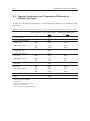
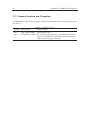
1
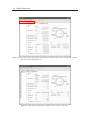
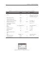
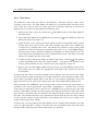
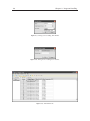
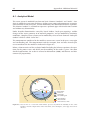
User Manual
TEMPEST
Computer Program for the Simulation of the
Wastewater Temperature in Sewers
Version 1.02
David J. Dürrenmatt and Oskar Wanner
[email protected]
http://www.tempest.eawag.ch
Atmosphere
Wastewater
Sewer air
Sewer pipe
Soil type 1
Soil type 2
Airflow
Wastewater discharge
Heat transfer
Mass transfer
Sources / sinks
System boundary
Lateral
inflow
Biofilm
Node 1
Node 2
Conduit 1
Node 3
Conduit 2
Conduit 3
Contents
1. Introduction
1.1.
1.2.
1.3.
1.4.
Background . . . . .
Program Capabilities
System Prerequisites
File Format . . . . .
1
.
.
.
.
.
.
.
.
.
.
.
.
.
.
.
.
.
.
.
.
.
.
.
.
.
.
.
.
.
.
.
.
.
.
.
.
.
.
.
.
.
.
.
.
.
.
.
.
.
.
.
.
.
.
.
.
.
.
.
.
.
.
.
.
.
.
.
.
.
.
.
.
.
.
.
.
.
.
.
.
.
.
.
.
.
.
.
.
.
.
.
.
.
.
.
.
.
.
.
.
.
.
.
.
.
.
.
.
.
.
.
.
.
.
.
.
.
.
.
.
.
.
.
.
1
1
2
2
2.1. Overview . . . . . . . . . . .
2.1.1. User Interface . . . . .
2.1.2. File Handling . . . . .
2.2. Model Formulation . . . . . .
2.2.1. Sewer Lines . . . . . .
2.2.2. Time Series . . . . . .
2.2.3. Model Settings . . . .
2.3. Computation . . . . . . . . .
2.3.1. Steady State Solutions
2.3.2. Dynamic Solutions . .
2.3.3. Computation Process .
2.3.4. Numerical Parameters
2.4. Results: View and Export . . .
2.5. System Preferences . . . . . .
.
.
.
.
.
.
.
.
.
.
.
.
.
.
.
.
.
.
.
.
.
.
.
.
.
.
.
.
.
.
.
.
.
.
.
.
.
.
.
.
.
.
.
.
.
.
.
.
.
.
.
.
.
.
.
.
.
.
.
.
.
.
.
.
.
.
.
.
.
.
.
.
.
.
.
.
.
.
.
.
.
.
.
.
.
.
.
.
.
.
.
.
.
.
.
.
.
.
.
.
.
.
.
.
.
.
.
.
.
.
.
.
.
.
.
.
.
.
.
.
.
.
.
.
.
.
.
.
.
.
.
.
.
.
.
.
.
.
.
.
.
.
.
.
.
.
.
.
.
.
.
.
.
.
.
.
.
.
.
.
.
.
.
.
.
.
.
.
.
.
.
.
.
.
.
.
.
.
.
.
.
.
.
.
.
.
.
.
.
.
.
.
.
.
.
.
.
.
.
.
.
.
.
.
.
.
.
.
.
.
.
.
.
.
.
.
.
.
.
.
.
.
.
.
.
.
.
.
.
.
.
.
.
.
.
.
.
.
.
.
.
.
.
.
.
.
.
.
.
.
.
.
.
.
.
.
.
.
.
.
.
.
.
.
.
.
.
.
.
.
.
.
.
.
.
.
.
.
.
.
.
.
.
.
.
.
.
.
.
.
.
.
.
.
.
.
.
.
.
.
.
.
.
.
.
.
.
.
.
.
.
.
.
.
.
.
.
.
.
.
.
.
.
.
.
.
.
.
.
.
.
.
.
.
.
.
.
.
.
.
.
.
.
.
.
.
.
.
.
.
.
.
.
.
.
.
.
.
.
.
.
.
.
.
3
3
5
5
6
9
11
12
12
14
14
14
15
18
3.1. Introduction . . . . . . . . . . . . . . . . .
3.2. Field Measurements and Data Acquisition
3.3. Modeling with TEMPEST . . . . . . . . . .
3.3.1. Model Calibration . . . . . . . . .
3.3.2. Model Validation . . . . . . . . . .
3.3.3. Heat Recovery Scenarios . . . . . .
3.4. Conclusions . . . . . . . . . . . . . . . . .
.
.
.
.
.
.
.
.
.
.
.
.
.
.
.
.
.
.
.
.
.
.
.
.
.
.
.
.
.
.
.
.
.
.
.
.
.
.
.
.
.
.
.
.
.
.
.
.
.
.
.
.
.
.
.
.
.
.
.
.
.
.
.
.
.
.
.
.
.
.
.
.
.
.
.
.
.
.
.
.
.
.
.
.
.
.
.
.
.
.
.
.
.
.
.
.
.
.
.
.
.
.
.
.
.
.
.
.
.
.
.
.
.
.
.
.
.
.
.
.
.
.
.
.
.
.
.
.
.
.
.
.
.
20
21
23
27
29
29
30
2. Program Handling
3
3. Case Study
20
Bibliography
33
A. Additional Material
A.1. Analytical Model . . . . . . . . . . . . . . . . . .
A.1.1. Balance Equations and Transfer Processes
A.1.2. Nodes . . . . . . . . . . . . . . . . . . . .
A.2. PDE Solver . . . . . . . . . . . . . . . . . . . . .
B. Material Properties
35
.
.
.
.
.
.
.
.
.
.
.
.
.
.
.
.
.
.
.
.
.
.
.
.
.
.
.
.
.
.
.
.
.
.
.
.
.
.
.
.
.
.
.
.
.
.
.
.
.
.
.
.
.
.
.
.
.
.
.
.
36
37
37
40
41
B.1. Friction Coefficients kst . . . . . . . . . . . . . . . . . . . . . . . . . . . . . . 42
B.2. Thermal Conductivity and Temperature Diffusivity of Different Pipe Types . 43
B.3. Thermal Conductivity and Temperature Diffusivity of Different Soil Types . . 44
i
ii
Contents
C. TEMPEST Development
45
C.1. Program Versions and Changelog . . . . . . . . . . . . . . . . . . . . . . . . 46
1
Introduction
The program TEMPEST was designed for the calculation of the dynamics and longitudinal
spatial profiles of the wastewater temperature in the sewer. This manual introduces the
concepts behind TEMPEST and explains the program handling. It is organized as follows:
It first discusses the program’s fields of application, its capabilities and the system prerequisites. The second chapter focuses on the program handling and explains the conceptual
model formulation. Chapter 3 exemplifies the application of TEMPEST in a heat recovery
project for the assessment of the recoverable amount of heat.
1.1. Background
Raw wastewater contains a considerable amount of energy which can be recovered and
used to produce warm water and for room heating. This is done by means of a heat pump
and a heat exchanger which is installed in the sewer.
The optimal location for the installation of a heat exchanger in the sewer depends on
several criteria. First of all, it is important that the energy consumers are located close
to the site where the heat is recovered. More heat can be reclaimed from the wastewater
if the discharge is high, which is typically the case towards the end of the sewer. On
the other hand, the wastewater temperature usually is highest in the initial part of the
sewer system. An additional aspect to be considered is that the efficiency of a nitrifying
wastewater treatment plant is reduced if its influent wastewater temperature is lowered
(Wanner et al., 2005). Therefore, planning and design of facilities for heat recovery from
raw wastewater require that the changes of the wastewater temperature along the flow
path in the sewer and the effect of heat recovery on the influent temperature of wastewater
treatment plants can be quantified.
The interactive simulation program TEMPEST (temperature estimation) has been developed to calculate the dynamics and longitudinal spatial profiles of the wastewater temperature in the sewer. The program is based on a new model of the heat balance in sewers
(Dürrenmatt, 2006 and for a summary of the model equations see Appendix A.1). Applications range from simple steady state estimates of the changes of the wastewater temperature in a single sewer line to full scale simulations of the dynamics of the wastewater
temperature in successive sewer lines with lateral inflows.
1.2. Program Capabilities
TEMPEST targets high applicability in practice. The implemented model requires as few
input data and a priori estimates as possible. TEMPEST applies default values wherever
1
2
Chapter 1. Introduction
possible and disposes of a library that already contains parameter values for the most common soil and pipe types. Generally, it prefers parameters that are either easy to measure
or available from the literature, and internally converts them into the appropriate format.
However, the model includes all processes, which are of primary importance. Its clear and
intuitive graphical user interfaces make it easy to handle.
Some among the major capabilities are:
• The sewer hydraulics is modeled with the dynamic form of the St. Venant equations
(Cunge et al., 1980). Therefore, the user has to provide upstream discharge data
only. To model parameters, such as temperature, humidity and airflow, balance equations which form a system of one-dimensional partial differential equations (PDEs)
are used (for an overview, see Appendix A.1).
• To yield high accuracy and numerical stability, the two step Lax-Wendroff algorithm
(Press, 2005) is implemented to solve the system of PDEs (for implementation details, please refer to Appendix A.2).
• TEMPEST applications range from simple steady state estimates of the changes of
the wastewater temperature in a single sewer line to full scale simulations of the
dynamics of the wastewater temperature in large systems of successive sewer lines
with lateral inflows.
• Intuitive graphical user interfaces assist the user in managing data, performing calculations and plotting results. Data can easily be imported from a text file or spreadsheet and results can be plotted on the screen and exported for further use.
1.3. System Prerequisites
TEMPEST is written in the object oriented programming language C++ and uses the
wxWidgets graphical user interface library. It is compiled for the Microsoft Windows operating systems and consists of just one executable file, has no dependencies on external
libraries and does not require any software installation. Therefore, the only action to be
taken in order to run the application is to copy or download the executable file and execute
it.
The program has been extensively tested on Windows XP and Windows Vista but it should
also run on previous versions of Windows. Since it numerically solves partial differential
equations and therefore performs a lot of calculations, faster processor clocks yield shorter
calculation times.
1.4. File Format
Models created with TEMPEST can be saved to disk and have the extension “tmo”. Sewer
line definitions, material parameters and time series data as well as numerical settings will
be saved. Therefore, TEMPEST model files can conveniently be exchanged between users
and platforms.
2
Program Handling
The handling of TEMPEST and its dialog boxes are illustrated in
this chapter. The model formulation is explained and it is shown,
how sewer systems can be modeled in TEMPEST. The order of the
sections corresponds to a typical session in which a user first creates a model file, then defines the model, performs and optimizes
computations and eventually analyzes the results.
2.1. Overview
2.1.1. User Interface
Figure 2.1 shows the main window of TEMPEST upon the start of the program. The
commands for file handling, model creation and editing and computation can be found in
the menus of the menu bar. The commands most often used also are represented in the
toolbar. All commands are listed and described in Table 2.1.
P
P Menubar
P
P
Toolbar
Figure 2.1.: Main window of TEMPEST.
3
4
Chapter 2. Program Handling
Table 2.1.: Menu and toolbar items.
Menu item
Hot key
File
Alt + F
New
Toolbar icon
Ctrl + N
See also
2.1.2
Open...
2.1.2
Close
Ctrl + W
Save
Ctrl + S
Save As...
Ctrl + Shift + S
–
2.1.2
2.1.2
–
2.1.2
Export Data...
–
2.4
Recent Files...
–
Exit
Edit
Alt + F4
–
Alt + E
–
Copy
–
2.2.2
Paste
–
2.2.2
Preferences
–
2.5
Model
Alt + M
Add Sewer Line
2.2.1
Remove Sewer Line
2.2.1
Add Time Series
2.2.2
Delete Time Series
2.2.2
Insert Column
2.2.2
Remove Column
2.2.2
Validate Entries and Data
Model Settings...
Compute
–
Alt + C
2.2.3
–
Steady State Solution
2.3
Dynamic Solution
2.3
View
Alt + V
–
Sewer Lines
–
2.2.1
Time Series
–
2.2.2
Results
–
2.4
Box Zoom
2.4
Pan
2.4
Zoom In
2.4
Zoom Out
2.4
Restore View
2.4
Help
About...
Alt + H
–
2.2. Model Formulation
5
2.1.2. File Handling
TEMPEST models (consisting of sewer lines, time series and settings) are stored in model
files with the file extension TMO.
The File menu provides the basic functionalities to create TEMPEST models (File – New),
to save a model (File – Save or File – Save As...) or to load a previously created model
from the file system (File – Open...).
2.2. Model Formulation
In TEMPEST, the basic element used to build models of complex sewer systems, is the
“Sewer Line”, which consists of a “Node” followed by a “Conduit” (Dürrenmatt and Wanner, 2008). Nodes are introduced in the sewer at each location, where there are lateral
inflows, changes in the pipe geometry, changes in the material properties of the sewer
pipe, or changes in the surrounding soil, as shown in Figure 2.2. Lateral wastewater inflows to the system and inflow temperatures can either be constant values in time or time
series.
Mathematically, “Conduits” represent sets of mass balance equations and “Nodes” represent sets of continuity conditions of the variables of successive conduits. The variables
considered are discharge and temperature in the wastewater compartment, airflow, temperature and humidity in the sewer headspace, and temperature in the sewer pipe and
the surrounding soil. The hydraulics is modeled with the St. Venant equations (Cunge
et al., 1980) and the airflow with a recently developed model for circular pipes. The heat
and mass transfer processes considered in the model are shown in Figure 2.3. The rate
expressions of the transfer processes were taken from the literature (e.g. Holman, 2002;
Incropera and DeWitt, 2002; Wanner et al., 2004). The complete mathematical model implemented in TEMPEST is described and discussed in two publications (Dürrenmatt, 2006
and Wanner and Dürrenmatt, in preparation; an overview is given in Appendix A.1).
The following sections explain how to input sewer lines and read in time series data.
Unsaturated soil
Sewer line =
Node +
Saturated soil
Conduit
Flow direction
Air exchange
N
Figure 2.2.: Discontinuities require that nodes are introduced, which separate sewer conduits having different
properties.
6
Chapter 2. Program Handling
Atmosphere
Wastewater
Sewer air
Sewer pipe
Soil type 1
Soil type 2
Airflow
Wastewater discharge
Heat transfer
Mass transfer
Sources / sinks
System boundary
Lateral
inflow
Biofilm
Node 1
Node 2
Conduit 1
Node 3
Conduit 2
Conduit 3
Figure 2.3.: Compartments and processes considered in the sewer model. Complex systems can be modeled
by series of the elements "node plus conduit".
2.2.1. Sewer Lines
Each model can contain an unlimited number of sewer lines. The management of the
sewer lines is done within the Sewer Lines tab (see Figure 2.4): The Table to the left lists
the successive sewer lines, the form to the right has input fields for the various parameters.
A small image of a sewer cross section with the location where each model parameter is
measured indicated helps the user.
In TEMPEST, the input data needed for wastewater temperature simulations can be divided into three groups: sewer node data, sewer pipe data and surrounding soil data.
The wastewater discharge and temperature, ambient meteorological conditions, and the
Air Exchange Coefficient at the upstream end of a sewer conduit are specified in the Sewer
Node section. The Air Exchange Coefficient describes the capacity for air exchange between
the sewer and the environment. The Sewer Pipe and Soil sections are filled with data
describing these two compartments. By the select fields the user can choose appropriate
values for thermal conductivities, a biofouling factor and friction coefficients of many types
of materials. The COD Degradation Rate describes the production of heat by biological
processes and the Penetration Depth describes the depth to which the soil temperature
TS,inf is assumed to be affected by the sewer. Table 2.2 lists all parameters needed to
model a sewer system with TEMPEST and Figure 2.5 shows a screenshot of the Sewer
Lines form with typical parameter values.
in the toolbar or, alternatively, select Add Sewer Line...
To add a new sewer line, click on
from the Model menu. A dialog box as shown in Figure 2.6 appears. You can now name
the series and, if desired, choose a sewer line whose parameter values should be copied
and used for the new sewer line. Confirm by clicking the OK button.
Sewer lines can be deleted by using the Remove Sewer Line command from the Model
menu or by using the
button in the toolbar.
2.2. Model Formulation
7
PP
P
P Model tabs
Figure 2.4.: New model with empty Sewer Lines form. The model tabs can be used to switch between Sewer
Lines, Time Series and Results view.
Figure 2.5.: Main window displaying the Sewer Lines tab completed with values.
8
Chapter 2. Program Handling
Table 2.2.: List of all parameters needed in order to perform simulations with TEMPEST.
Name
Symbol
Unit
Constraints
Inflow
QWin
m3 /s
QWin > 0 m3 /s for first
and QWin ≥ 0 m3 /s for
successive sewer lines
Inflow Temperature
TWin
°C
TA
°C
phiA
–
0 ≤ phiA ≤ 1
pA
mbar
pA > 0 mbar
b
–
Sewer Node
Ambient Temperature
Ambient Relative Humidity
Ambient Air Pressure
Air Exchange Coefficient
0≤b≤1
Sewer Pipe
Type
(kst, lambdaP, aP, f)
Value from library
Length
L
m
L>0m
Nominal Diameter
D
m
D>0m
Wall Thickness
s
m
s>0m
S0
–
S0 > 0
r
mg/(m3 s)
Slope
COD Degradation Rate
Soil
Type
(lambdaS, aS)
Value from library
Penetration Depth
deltaS
m
Soil Temperature
TS,inf
°C
Figure 2.6.: Dialog box for adding new sewer lines.
deltaS > 0 m
2.2. Model Formulation
9
2.2.2. Time Series
The inflow of a sewer line can either be described by a constant value or a time series.
To define a time series, the Time Series tab which has a spreadsheet-like interface can be
used. If the user wants to add a new time series for wastewater discharge or wastewater
temperature, he or she has to perform the following steps:
1. Switch to the time series tab (click on the
the View menu).
Time Series tab or select Time Series in
2. Select Add Time Series in the Model menu or click on
dialog box showed in Figure 2.7.
in the toolbar to open the
3. Name the time series, specify the initial number of rows (corresponds to the number
of data point you want to enter) and select whether your time series should have
a relative or an absolute time scale. The former has seconds as unit starting from
second zero, whereas the latter uses absolute time values (e.g. “25.02.2004 12:00”).
The time series is then added by clicking the OK button. Its name appears in the list
on the left of the Time Series tab and is automatically selected. The time series now
consists of a column for time values only.
in the toolbar
4. In order to add a column for inflow or inflow temperature, click on
or open the Model menu and select Insert Column... and specify the parameter you
want to add to column for and a default value (not required). Figure 2.8.
5. Repeat step 4 to add another column and go to step 2 to add additional time series.
If new time series are added, the appropriate select fields in the Sewer Lines tab will
be extended.
To input and edit values, two main methods can be applied: The user can use the arrow
keys or the mouse cursor to navigate in the table and enter values directly or, more easily,
paste values previously copied from a text file or a spreadsheet application (select the
upper left cell were the pasted area should start and select Paste from the Edit menu).
Please consider that TEMPEST expects the date/time values to have the same format as
specified in the system preferences (menu Edit – Preferences...) and that date and time
values must be provided. If this is not the case, TEMPEST tries its best to guess the right
format. Furthermore, consider that data gaps are not allowed and that the date/time value
must increase with increasing row number. The program ignores empty cell at the end of
the table. The columns for time series parameters do not need to have the same number
of rows but the number of rows of the time scale column must be at least as high as the
length of the longest data column.
In Figure 2.9, the screenshot of the Time Series tab of a model which contains one time
series (“25.02-27.02.08”) is shown. The time series has an absolute time scale and values
for both inflow discharge and inflow temperature are specified.
10
Chapter 2. Program Handling
Figure 2.7.: Dialog box for adding Time Series.
Figure 2.8.: Dialog box for adding new columns.
Figure 2.9.: Time Series tab.
2.2. Model Formulation
11
Time series columns and entire time series can be deleted if no references to sewer lines
exist.
• To delete a column of a time series, select the time series and click on
in the
toolbar or select Remove Column from the Model menu alternatively. Then, a dialog
box shows up listing the columns of the current time series. Select the column you
want to be removed and confirm your choice.
• In order to delete an entire time series, be sure that it is selected and click on
the toolbar (or menu Model – Delete Time Series).
in
2.2.3. Model Settings
The model settings dialog box includes data on material properties and numerical parameters. It can be opened by choosing Model Settings... from the Model menu. This dialog
box has three tabs, the first two tabs allow the user to add and modify data for pipe (Pipe
Types, Figure 2.10) and soil types (Soil Types, Figure 2.11), the third one lets the user
change the numerical parameters. The numerical parameters will be widely discussed in
Section 2.3.4. A selection of parameter values of the most common pipe and soil types is
given in Appendix B.
The forms to edit pipe and soil types have the same user interface but the two types
have different parameters. Types can be added and removed by clicking on the respective
button indicated in Figure 2.10. In order to edit one of the types, select it in the list on top
of the dialog box and change the parameter values in the text fields below. The changes
are applied if the user clicks on the OK button.
Remove type
Add type 6
MBB
Figure 2.10.: Pipe Types tab of the Model Settings dialog box.
12
Chapter 2. Program Handling
Figure 2.11.: Soil Types tab of the Model Settings dialog box.
2.3. Computation
If the model formulation is complete, calculations can be performed. To open the Compute
Solution dialog box, either select Steady State Solution... or Dynamic Solution... in the
Compute menu, or click on
in the toolbar.
Before the Compute Solution dialog box is displayed, TEMPEST verifies the model (the
verification can also be manually started by clicking on
in the toolbar or by selecting
Validate Entries and Data in the Model menu).
If errors are found, the Verification Errors dialog box (Figure 2.12) appears. Each error is
listed, its category is illustrated with an icon and the sewer line parameter, the time series
data point, or the setting where it occurred is given. Once all the errors are corrected,
computations can be performed.
2.3.1. Steady State Solutions
The same dialog box is used to compute both steady state and dynamic solutions. A radio
button allows changing the type of calculation within the dialog box. A configuration
ready to perform a steady state simulation is shown in Figure 2.13.
If time series are used in the model, care has to be taken when filling in the Reference
Time: The reference time defines the link between the simulation time in the program and
the data for inflow, inflow temperature, or both. If all time series used have a relative time
scale, the reference time has the unit seconds. If all time series used have an absolute time
scale, the reference time must have a value as illustrated in Figure 2.13. If relative and
absolute time scales are mixed, an absolute date and time must be specified and the time
series with relative time scales are shifted to start with the reference time specified.
2.3. Computation
13
Figure 2.12.: Dialog box that displays errors.
Figure 2.13.: Dialog box for defining computation type and reference time to compute a steady state solution.
14
Chapter 2. Program Handling
TEMPEST uses linear interpolation algorithms to calculate values between known data.
The first value of the time series is taken for calculation times earlier than the first data
value and vice versa for computation times beyond the last data value of a time series.
2.3.2. Dynamic Solutions
In Figure 2.14, the dialog box of Figure 2.13 is set up for a dynamic calculation. Here, the
same rules for time series apply as discussed in the previous paragraph. It has to be noted
that TEMPEST automatically calculates a steady state solution first in order to generate
initial conditions for the dynamic simulation. The reference time for the calculation of the
steady state solution is set equal to the start time of the dynamic simulation.
In addition to a Start Time and an End Time, one can also choose the Output Timestep: It
specifies the temporal interval by which calculated results will be stored for further use.
2.3.3. Computation Process
Once the calculations have started, a dialog box with a progress bar appears (Figure 2.15)
and informs the user about the ongoing process. Usually, TEMPEST occupies a lot of processor time and the ability to work with other application while calculating can be limited
(this is defused if a multi core processor or multiple processors are at your disposition).
Therefore, the calculations can be paused and resumed by clicking on the Pause button
and ended by clicking on the Abort button.
If the steady state can not be found or the convergence is beyond the tolerance, TEMPEST
stops the calculation and gives advice for further optimization of the numerical parameters.
When finished, the dialog box with additional information, such as total computation time,
stays on the screen until it is closed.
2.3.4. Numerical Parameters
TEMPEST tries to guess the best suiting numerical parameters, though numerical settings
can still be modified by the user to improve accuracy and optimize calculation time. These
Figure 2.14.: Dialog box for defining computation type and reference time to compute a dynamic solution.
2.4. Results: View and Export
15
Figure 2.15.: Progress dialog showing typical information on the ongoing process of a dynamic solution.
Figure 2.16.: Dialog box for editing numerical settings.
settings can be accessed in the Numerics tab of the Model Settings dialog box (Figure
2.16). To open the dialog box, click on Model Settings... in the Model menu and select the
appropriate tab, or click on the Numerical Settings button in the Compute Solution dialog
box (Figure 2.13 and Figure 2.14).
Three groups of parameters can be modified: Parameters for the Newton-Raphson iterator,
the soil module structure and the PDE solver (cf. Appendix A.2). The parameters together
with a short description and the implemented default values are given in Table 2.3.
The numerical settings are stored together with the model in the TEMPEST file “Modelname.tmo”.
2.4. Results: View and Export
The results of a computation are displayed in the Results tab (Figure 2.17). It consists of
five sub panels:
16
Chapter 2. Program Handling
Table 2.3.: List of the numerical parameters needed by simulations performed with TEMPEST.
Parameter
Description
Default value
Newton-Raphson Iterator
Tolerance for Convergence
This is a relative value which specifies the accuracy that must be obtained in order to stop the iteration.
0.001
Defines the discretization of the
pipe in radial direction: the number of radial layers the pipe will be
divided in.
5
Max. Courant Number
If the step size in time is auto
computed, the solver tries to keep
the Courant number lower than the
given value.
0.95
Rel. Tolerance Steady State
Defines the relative tolerance which
must be reached for the solver to
abort the relaxation for steady state.
5x10⁻⁵
Max. Iterations (Steady State)
If steady state cannot be reached,
the solver will stop after this number of steps.
10 000
Stepsize in Space
Defines the spatial discretization
along the flow path in the sewer.
10 metres
Stepsize in Time
The discretization in time can either
be automatically computed or specified by the user.
(autocompute)
Apply Filter
To improve stability and avoid numerical artifacts, a non linear filter can be applied to suppress high
frequency oscillations of calculated
variables.
Enquist 2.1
Pipe/Soil Module Structure
Number of Pipe Layers
PDE Solver
2.4. Results: View and Export
17
Figure 2.17.: Main window displaying the calculation Results tab. The wastewater and sewer air temperature
as well as the temperature of the pipe layers are plotted.
18
Chapter 2. Program Handling
• Data selection (top left and bottom left): Either the time or the location for which
the results are to be plotted and listed can be selected.
• Data table (bottom right): Lists the numerical values of the data series for the time
value or location selected.
• Plot panel (top center): Visualizes the listed data.
• Data series panel (top right): The user can select the data series to be plotted.
Several tools are at your disposition to navigate and zoom within the plot panel. The
mouse cursor can either be in box zoom state or pan state. In order to switch between
and the
icon in the toolbar. If the box zoom state is activated, a
these states use the
rectangular box can be drawn into the plot area which will then be zoomed in. If the mouse
cursor is in pan state, the clipping can be shifted (click and hold left mouse button while
moving). The
and
commands can be used to zoom in and zoom out, respectively. To
restore the original view, click on .
Cells, rows, columns or the entire data table can be selected and the selection may then
be copied to the clipboard (menu Edit – Copy).
The calculated values can also be exported for external use. Figure 2.18 shows the Data
Export dialog box (File menu - Export Data...) in which the variables, time and location as
well as output format can be specified. One can export spatial data for a given time step,
time series data at a fixed coordinate or all data together.
2.5. System Preferences
System preferences such as plot pen colors and the default date/time format can be
changed in the Preferences dialog box (Figure 2.19). To open it, select Preferences...
in the Edit menu.
Figure 2.18.: Dialog box for selecting data to export.
2.5. System Preferences
Figure 2.19.: Dialog box for editing the system preferences.
19
3
Case Study
In this chapter, it is illustrated step by step how TEMPEST can be
used for the optimal planning of heat recovery from the sewer. It is
described, which data must necessarily be collected and it is shown,
how a TEMPEST model is created, calibrated and validated, and
then is used for the modeling of load scenarios.
3.1. Introduction
A fictitious heat recovery project was defined as follows: It is planned to erect a new
building close to manhole RS 4943 in Rümlang (see Figure 3.1). Since a lot of attention
is given to ecological aspects during all phases of the building project, the project team
also wants to assess the potential of using heat that is reclaimed from the wastewater of a
sewer system situated nearby for room heating and warm water production.
In this fictitious project, TEMPEST is used to model the sewer system and to calculate
different heat recovery scenarios. For each scenario, one must check that the legal constraints are fulfilled. Those constraints assure that there will be no negative effects for the
downstream wastewater treatment plant due to the heat recovery (here, we assume that
the plant is located right after manhole RS 3096, 1.845 km downstream of RS 4943). In
the Canton of Zurich, the inflow temperature to the plant must not fall below 8 °C and
the maximum temperature decrease resulting from temperature reclamation must not be
higher than 0.5 °C (AWEL, 2003).
The preparatory work before being able to model the sewer system with TEMPEST is discussed in Section 3.2. Then, it is illustrated how the considered section of the Rümlang
Oberglatt
Manhole
RS 3096
Rümlang
Manhole
RS 4943
L=
184
5m
ion
rect
di
Flow
500 m
Figure 3.1.: Top view of a section of the sewer between the villages Rümlang and Oberglatt in the Canton of
Zurich, Switzerland
20
3.2. Field Measurements and Data Acquisition
21
sewer system can be modeled in TEMPEST (Section 3.3) and how calibration (Section
3.3.2) and validation (Section 3.3.2) are performed using the available data. Two exemplary heat recovery scenarios are simulated in Section 3.3.3. Finally, some conclusions
drawn from the project are addressed in Section 3.4.
3.2. Field Measurements and Data Acquisition
In order to model the considered sewer section with TEMPEST, geometrical as well as
material properties must be known. Further, discharge and temperature measurements
and meteorological data must be measured, gathered or estimated for the period in time
which will be used for model calibration and validation.
For the Rümlang sewer, data were measured by an ultrasonic flow meter and a temperature logger mounted at RS 4943 manhole and a temperature logger in manhole RS 3096
(TEMPEST automatically calculates the hydraulics). The measured discharge and temperature data are plotted in Figure 3.2. To get a good estimate for the ground temperature,
a temperature logger was buried in 1.2 m depth and in 2 m distance from the sewer at
manhole RS 4943.
RS 4943
RS 3096
RS 4943
3
Discharge [m /s]
3
Discharge [m /s]
Information on the geometrical and material properties were made available by the engineering company that has built the sewer section. Based on the type of concrete that has
been used, the parameters of the thermal properties and the friction coefficient of the pipe
were estimated. The thermal properties of the soil were estimated based on the soil discovered on-site. Meteorological data were taken from the closest meteorological station.
The values of these parameters are listed in Table 3.1.
0.2
0.1
0
26−Feb−2008
27−Feb−2008
28−Feb−2008
Temperature [°C]
Temperature [°C]
12−Mar−2008
13−Mar−2008
14
12
8
26−Feb−2008
0.1
0
11−Mar−2008
14
10
0.2
RS 4943
RS 3096
27−Feb−2008
28−Feb−2008
12
10
8
11−Mar−2008
RS 4943
RS 3096
12−Mar−2008
13−Mar−2008
Figure 3.2.: Discharge and temperature data measured from February 26 to February 28 (left column) and
from March 11 to March 13 (right column) at the manholes RS 4943 and RS 3096.
22
Chapter 3. Case Study
Table 3.1.: Geometrical and meteorological parameters, and material properties that describe the sewer section RS 4943-RS 3096 in Rümlang. Estimates were made where no data was available. Key
to “Origin” column: IP=implementation plan, E=estimate, AS=ANETZ meteorological station,
L=literature (cf. Appendix B).
Parameter
Symbol
Value
Unit
Origin
Length
L
1845
m
IP
Nominal diameter
D
0.9
m
IP
Wall thickness
s
0.1
m
IP
Sewer slope
S0
0.0091
-
IP
Friction coeff.
kst
70
m1/3 s−1
E
Fouling factor
f
200
W/(m2 K)
L
COD degradation rate
r
0.6-2.8
mgCOD/(m3
Soil penetration depth
δS
0.1
m
E
Air exchange coeff.
b
0.1
-
E
Ambient temperature
TA
8.3
°C
AS
Ambient air pressure
pA
966
mbar
AS
Relative humidity
ϕ
0.75
-
AS
Soil temperature
TS,in f
5.5
°C
M/E
Thermal conductivity pipe
λP
0.3-2.5a
W/(m K)
IP / L
Thermal conductivity soil
λS
0.25-2.5b
W/(m K)
IP / L
Thermal diffusivity pipe
aP
0.4 - 0.6 a
m2 /s
IP / L
aS
b
m2 /s
IP / L
Thermal diffusivity soil
a Reinforced
b Gravel
0.3 - 0.8
concrete
with a porosity of 50% and 50% saturated
s)
L
3.3. Modeling with TEMPEST
23
Figure 3.3.: Main window of TEMPEST as it shows up when the TEMPEST executable file is run.
3.3. Modeling with TEMPEST
In order to simulate the effect of heat recovery at the upstream site on the downstream
wastewater temperature a new model has to be setup and the parameters of the sewer
section and the time series data must be entered into the model. To do so, run the TEMPEST executable file in Windows. The main window as shown in Figure 3.3 appears. After
selecting New from the File menu, a model is created but does not yet contain any sewer
line or time series. Since the relevant data needed is already at the user’s disposition, he
or she can start to define sewer lines now.
Between manhole RS 4943 and RS 3096, there are actually around 30 additional manholes. Ideally the sewer should be modeled by 31 sewer lines separated by the manholes.
However, since there are no relevant parameter changes along the flow path, and since the
manhole covers only have small openings with very limited air exchange, it is sufficient to
set up the TEMPEST model with just one sewer line of 1845 m in length.
After clicking on Add Sewer Line in the Model menu, a dialog box appears. In this box
a name (e.g. “Rümlang”) for the new sewer line can by typed in and it can be chosen
whether or not the parameters are to be copied from an already existing line (since you
are adding the first line now, the dropdown list is still empty). The new sewer line is added
by clicking on OK and is now listed on the left side of the sewer lines tab (see Figure 3.4).
You may rename the sewer line at any time later by clicking its name.
The data of the Rümlang sewer as given in Table 3.1 can now be entered into the Sewer
Lines form. For Inflow and Inflow Temperature, the user can either enter a constant value
or define a time series. Because the objective of this project is to choose an heat extraction mode that does not negatively affect the performance of the downstream wastewater
treatment plant but that reclaims as much heat as possible, the amount of heat extracted
is most certainly not constant over time. Thus, a dynamic simulation must be performed
and therefore the latter be selected.
After clicking on the Time Series radio button for QWin in the Sewer Node panel of the
Sewer Lines tab, you can access a drop down list. Initially, there are no values in the list
because no time series has been added to the TEMPEST model yet. To add a new time
series, click on Add Time Series from the Model menu. A dialog box appears that lets you
24
Chapter 3. Case Study
Figure 3.4.: The Sewer Lines tab. A new, empty sewer line has been added to the model and the parameter
values of Table 3.1 have been entered.
3.3. Modeling with TEMPEST
25
Figure 3.5.: The newly added time series which is named “Measuring Campaign 26.2-28.2.2008” is now
available in the list to the left. The time series data table currently only has a Date / Time row.
name the series (e.g. “Measuring Campaign 26.2-28.2.2008”), define the number of rows
the time series table should have (e.g. 1000) and choose between a relative time scale,
where the time series starts from second zero, and an absolute time scale, depending on
the time format of the measured time series data. Select Absolute (Date/Time). The time
series tab is now visible showing the Date / Time column of the added time series (Figure
3.5).
Before adding inflow and temperature data to the data table, a new column must be added
for each of the two variables. This is done by selecting Insert Column from the Model
menu, for both, the Lateral Inflow [m3/s] and the Lat. Inflow Temperature [°C] parameter.
The Default Value field can be left blank. Note that Lateral Inflow also refers to the inflow
at the upper end of the sewer to be modeled.
In order to fill the cells of the time series table for long time series, it is recommended to
copy-paste the data from a text file or a spreadsheet application like MS Excel. Care has to
be taken that the date/time format in the data source is similar to the format specified in
the TEMPEST preferences (menu Edit – Preferences...). Once the data of the source file is
copied to the clipboard, you can select the upper left cell of the time series table and select
Paste from the Edit menu. The time series named “Measuring Campaign 26.2-28.2.2008”
is now filled with data as shown in Figure 3.6.
If you switch back to the Sewer Lines tab, you can now select the new time series in the
drop down lists for inflow and inflow temperature.
The last parameters to be set before you can start the model calibration are the sewer
pipe and soil type. Every TEMPEST model disposes of a pipe and soil type library which
can be accessed via the menu Model – Model Settings. Add a new pipe type in the Pipe
Types tab of the Model Settings dialog box and enter the estimates from Table 3.1 for the
friction coefficient, the thermal conductivity, the thermal diffusivity and the fouling factor
and assign a comprehensive label (Figure 3.7). The same steps can be performed to add
a new soil type to the library after switching to the Soil Types tab. Save the changes and
close the dialog by clicking on OK. In the Sewer Pipe panel and the Soil panel of the Sewer
Lines tab now select the appropriate Type for pipe and soil, respectively, from the list.
All the data needed to perform simulations has now been entered. If you want to verify
whether the model is complete, select Validate Entries and Data from the Model menu.
Before starting the model calibration, it is recommended to save the model file to disk
(File - Save).
26
Chapter 3. Case Study
Figure 3.6.: The data table of the series named “Measuring Campaign 26.2-28.2.2008” is filled with data
copied from a spreadsheet application.
Figure 3.7.: Pipe Types library with an entry for the Rümlang sewer pipe type. Since no exact values were
available, rough estimates have been typed in.
3.3. Modeling with TEMPEST
27
3.3.1. Model Calibration
In the model calibration phase, one tries to change to model parameters (within certain
limits) so that the output of the model, the simulated wastewater temperature at the lower
end of the sewer section, matches the measured temperature as good as possible.
The time series of the measuring period from February 26 to February 28 2008 (Figure 3.2,
page 21) will be used for the calibration. You can first try to calculate the downstream
wastewater temperature using the parameters given in Table 3.1. Click on Compute – Dynamic Solution to open the Compute Solution dialog. The option Compute dynamic solution
is preselected and start and stop times are set to the first and the last time series value
defined in the time series used in the model (Figure 3.8). The Output Timestep [s] can be
changed in order that more or less calculated data are saved as results.
Usually, there is no need to change the numerical settings (see Section 2.3.4). If your
sewer system is rather long but not very dynamic and complex, you can try to increase
the Stepsize in Space [m] in order to speed up the calculation time (click on Numerical
Settings...). If you want to find the optimal stepsize, start with a rather long stepsize and
perform the calculation. Now, decrease to stepsize gradually until the results of the actual
and the last calculation do not differ significantly.
By clicking on Run..., the calculation process starts. A progress bar keeps you informed
about the ongoing process. First, the steady state solution is calculated using the time
series values at the specified start time. The steady state solution is then used as initial
condition for the calculation of the dynamic solution. Since the heat transfer processes
in the sewer pipe and the soil are rather slow, the relaxation time of the steady state
calculation might be shorter than the time needed. A possible way to cope with this
phenomenon is to duplicate the input time series and perform a simulation, e.g. for 6 days
instead of the original 3 days of available input data, and use the results of the last 3 days
of the simulation only.
When the calculation process has finished, you can close the progress dialog. TEMPEST
will now show the Results tab. To compare the values of the calculated and measured
variables at the downstream end of the sewer, the calculated variables must be transferred
to a data analysis or spreadsheet application. You can either export the data by using
the Data Export dialog (File – Export Data..., cf. Section 2.4) or first choose the row “x
= 1845.00 m” in the Parameter vs Time list (lower left), then select the variable row by
clicking on its header in the data table (lower right) and select Copy from the Edit menu.
If the parameters TS,in f , λP , aP , λS , aS , and δS are systematically changed within the ranges
indicated in Table 3.1 on page 22, a good correspondence between the temperatures simulated and measured in Rümlang is achieved using the values listed in Table 3.2. The
measured and calculated time series are plotted in Figure 3.9.
28
Chapter 3. Case Study
Figure 3.8.: The Compute Solution Dialog.
Table 3.2.: Parameters changed during the model calibration and values yielding good correspondence of
measured and calculated data.
Parameter
Symbol
Value
Unit
Soil penetration depth
δS
0.11
m
Soil temperature
TS,in f
5.5
°C
Thermal conductivity pipe
λP
2.3
W/(m K)
Thermal diffusivity pipe
aP
0.5
m2 /s
Thermal conductivity soil
λS
0.7
W/(m K)
Thermal diffusivity soil
aS
0.6
m2 /s
15
14
Temperature [°C]
13
12
11
10
RS 4943
RS 3096 (measured)
RS 3096 (calculated)
9
8
26−Feb−2008
27−Feb−2008
Figure 3.9.: Result of the model calibration.
28−Feb−2008
3.3. Modeling with TEMPEST
29
15
RS 4943
RS 3096 (measured)
RS 3096 (calculated)
14
Temperature [°C]
13
12
11
10
9
8
11−Mar−2008
12−Mar−2008
13−Mar−2008
Figure 3.10.: Result of the model validation.
3.3.2. Model Validation
The model parameter values identified during the model calibration phase now have to
be validated by performing a simulation using time series data that have not already been
used for the model calibration. If the accuracy of the model validation, more precisely the
correspondence of the simulated and the measured downstream temperatures, is satisfying, the model can be accepted. Otherwise, the calibration must be revised.
In Figure 3.10, the results of a simulation based on the model parameters found by the
calibration and based on inflow and inflow temperature values from March 8 to March
9 2008, are compared to the corresponding measurements. The accordance of the two
series is satisfying.
3.3.3. Heat Recovery Scenarios
By comparing two very simple heat recovery scenarios, the potential of TEMPEST as a tool
to investigate the effects of heat recovery on the downstream wastewater treatment plant
is demonstrated.
In the first scenario, a constant amount of heat of Q̇rec = 350kW shall be reclaimed at the
upper end of the sewer (at manhole RS 4943) and used for the fictitious building planned
next to the manhole. In the second scenario the amount of heat extracted is varied during
the day: Q̇rec = 500kW from 7 am to 10 pm, and Q̇rec = 100kW from 10 pm to 7 am. The
total amount of heat recovered is the same for both scenarios.
When heat is recovered from wastewater, the wastewater temperature decreases. Given
the amount of heat extracted, Q̇rec , the wastewater temperature and discharge upstream
30
Chapter 3. Case Study
of the heat exchanger, TW,in and QW , respectively, the temperature after the heat exchanger
TW,out can be calculated using the equation
TW,out = TW,in −
Q̇rec
c p,W ρW QW
(3.1)
where c p,W stands for the specific heat capacity of water and ρW for the density of water.
In order to investigate the effect of the decrease of TW,out on the wastewater temperature
at the downstream end of the sewer, the new time series TW,out , stored, e.g. in an Excel
spreadsheet, can be used as input time series for the model developed above. To do so, add
a new time series in the Time Series tab, add the column for the wastewater temperature
and copy-paste the values of TW,out with the corresponding date/time values into the data
table (proceed as described in the model calibration section). Now, switch to the Sewer
Lines tab and select the new time series as input for the inflow temperature.
In Figure 3.11 the wastewater temperatures at the downstream end of the sewer (manhole
RS 3096) calculated for the two scenarios are compared. One can see that the first scenario
which reclaims a constant amount of heat causes cold downstream temperature peaks at
times where the discharge in the sewer is low (though there is even some warming up
during the flow time in the sewer). In contrast, the diurnal variation of the downstream
temperature calculated for the second scenario is much smaller.
Additional heat recovery scenarios could start from the second scenario and try to further
increase the amount of heat extracted, or to optimize the pattern of the diurnal extraction
profile.
3.4. Conclusions
By means of a simple and fictitious example, a procedure to use TEMPEST for planning of
heat recovery projects is proposed.
To achieve this, the data needed in order to model the sewer section has to be acquired.
Model parameters can be measured on-site or found in the literature. When data is missing, even a priori estimates may be used. Because TEMPEST yields model predictions
whose accuracy depend on the accuracy of the input data available, sensitivity analyses
can be performed in order to assess the accuracy of the predicted results.
Model calibration is used to adjust the model parameters to the specific conditions of the
sewer considered and model validation serves to test the reliability of the model predictions.
Once the model is set up and tested, it can be used, e.g., to estimate the effect of heat
recovery on the downstream wastewater temperature, to analyze alternative patterns of
heat recovery with diurnal variation or to identify potentially critical conditions for downstream wastewater treatment plants.
3.4. Conclusions
31
3
Discharge [m /s]
0
11−Mar−2008 12−Mar−2008 13−Mar−2008
0.4
0.3
0.2
0.1
0
11−Mar−2008 12−Mar−2008 13−Mar−2008
Extracted Heat [kW]
200
400
200
0
11−Mar−2008 12−Mar−2008 13−Mar−2008
3
400
600
Discharge [m /s]
Extracted Heat [kW]
600
11−Mar−2008 12−Mar−2008 13−Mar−2008
0.2
0.1
15
Temperature [°C]
Temperature [°C]
5
0.3
0
11−Mar−2008 12−Mar−2008 13−Mar−2008
15
10
0.4
10
5
11−Mar−2008 12−Mar−2008 13−Mar−2008
Figure 3.11.: Simulation results of two alternative heat recovery scenarios. In the first scenario (left column),
350 kW heat were constantly reclaimed from the wastewater. In the second scenario (right
column), 350 kW of were reclaimed from 7am to 10pm and 100 kW in the remaining time.
The discharge measured at the heat exchanger is plotted in the middle row. In the third row,
the temperature before the heat exchanger (dashed, black line), the temperature after the heat
exchanger (gray line) and the downstream temperature (bold, black line) are indicated.
Bibliography
AWEL, 2003. Wärmenutzung aus Abwasser: Kanalisation (ungereichnigt) und ARAAbläufe (gereinigt). AWEL-Standard.
Baehr, H. D., Stephan, K., 2006. Wärme- und Stoffübertragung, 5. Edition. Springer,
Berlin.
Bischofsberger, W., Seyfried, C., 1984. Wärmeentnahme aus Abwasser. Institut für
Bauingenieurwesen V (München) Lehrstuhl und Prüfamt für Wassergütewirtschaft und
Gesundheitsingenieurwesen, Institut für Siedlungswasserwirtschaft und Abfalltechnik
(Hannover).
Cunge, J., Holly, F., Verwey, A., 1980. Practical Aspects of Computational River Hydraulics.
Pitman.
Dürrenmatt, D. J., 2006. Berechnung des Verlaufs der Abwassertemperatur im Kanalisationsrohr. Diploma Thesis, ETH Zurich.
Dürrenmatt, D. J., Wanner, O., 2008. Simulation of the wastewater temperature in sewers
with TEMPEST. Water Science and Technology 57 (11), 1809–1815.
Hager, W. H., 1994. Abwasserhydraulik : Theorie und Praxis. Springer, Berlin.
Hohmann, R., Setzer, M. J., Wehling, M., 2004. Bauphysikalische Formeln und Tabellen.
Werner Verlag.
Holman, J. P., 2002. Heat transfer, 9. Edition. McGraw-Hill, New York.
Incropera, F. P., DeWitt, D. P., 2002. Fundamentals of heat and mass transfer, 5. Edition.
Wiley, New York.
Press, W. H., 2005. Numerical recipes in C++ the art of scientific computing, 2. Edition.
Cambridge University Press, Cambridge.
Scheffer, F., Schachtschabel, P., Blume, H.-P., 2002. Lehrbuch der Bodenkunde, 15. Edition. Spektrum Akademischer Verlag, Heidelberg.
Unsworth, M. H., Monteith, J. L., 1990. Principles of environmental physics, 2. Edition.
Edward Arnold, London.
VDI, 1963. VDI-Wärmeatlas Berechnungsblätter für den Wärmeübergang. VDI-Verlag, Düsseldorf.
33
34
Bibliography
Wanner, O., Dürrenmatt, D. J., in preparation. Heat recovery from sewers and its effect on
the influent temperature of wastewater treatment plants.
Wanner, O., Panagiotidis, V., Clavadetscher, P., Siegrist, H., 2005. Effect of heat recovery
from raw wastewater on nitrification and nitrogen removal in activated sludge plants.
Water Research 39 (19), 4725–4734.
Wanner, O., Panagiotidis, V., Siegrist, H., 2004. Wärmeentnahme aus der Kanalisation –
Einfluss auf die Abwassertemperatur. Korrespondenz Abwasser 51 (5), 489–495.
A
Appendix:
Additional Material
This appendix contains additional material, mainly on the analytical
model (model equations and transfer processes) implemented in
TEMPEST. Additionally, the algorithm used to numerically solve the
partial differential equations is introduced.
35
36
Appendix A: Additional Material
A.1. Analytical Model
The sewer system is modeled based on two basic elements “conduits” and “nodes”. Conduits, in which the wastewater discharge, airflow, water vapor and temperature are continuous functions in time and space, and are modeled by one-dimensional balance equations.
The element “conduit” is assumed to represent a prismatic pipe with circular cross-section
and without any discontinuity.
Nodes describe discontinuities caused by lateral inflows, head space openings, sudden
changes of the sewer geometry or of material properties, and are modeled by continuity
conditions. Complex sewer systems can be modeled by series of basic elements “node plus
conduit” which is called “sewer line”.
The compartments considered in the model are wastewater, sewer head space, sewer pipe
and surrounding soil. The compartments and the transport, heat and mass transfer processes considered in the model are indicated in Figure A.1.
Below, a short overview of the analytical model including the balance equations, the equations for the process rates and details on the modeling of the nodes is given. For more
detailed explanations, the reader is referred to Dürrenmatt (2006) and Wanner and Dürrenmatt (in preparation).
.
qcP
.
q PL
.
q cL‘
D/2
s
Biofilm
.
q WL
.
q eW
.
q‘COD
δB
.
q PW
Wastewater
Sewer air
Sewer pipe
Surrounding soil
Heat transfer
Mass transfer
Heat sources / sinks
Figure A.1.: Cross-section of a sewer line with transfer processes by which the humidity in the sewer
headspace and the temperatures in the wastewater, sewer headspace, sewer pipe and soil are
affected.
A.1. Analytical Model
37
Table A.1.: Balance equations which are solved by TEMPEST. The mathematical formulation of the heat and
mass transfer processes ( j̇ and q̇) can be found in Table A.2. The underlying assumptions are
discussed in depth in Dürrenmatt (2006) and Wanner and Dürrenmatt (in preparation). The
mass and the momentum balance equations of water are known as the St. Venant equations.
Mass Balances
Water discharge (QW )
Sewer airflow (QL )
Water vapor loading (X )
∂ QW
∂ AW
1
∂ t = − ∂ x − ρW jvP P
∂ QL
∂ AL
∂t = − ∂ x
∂ (AL X)
= − ∂ (Q∂Lx X) + ρ1W
∂t
( jvP P − jkP UL − jkL ′ AL )
Heat Balances
Water temp. (TW )
Sewer air temp. (TL )
( j)
Pipe layer temp. (TP )
∂ (AW TW )
= − ∂ (Q∂Wx TW ) + c p,W1 ρW (q̇PW UW − q̇W L P − q̇vP P + q̇ω ′
∂t
∂ (AL TL )
= − ∂ (Q∂Lx TL ) + c p,L1 ρL (q̇PL UL + q̇W L P + ξ q̇kL ′ AL )
∂t
( j)
( j)
∂ AP TP
( j+1/2)
( j+1/2)
( j−1/2) ( j−1/2)
1
q̇
U
−
q̇
=
U
P
P
P
P
c p,P ρP
∂t
AW )
Momentum Balance
Water
∂ QW
∂t
= − ∂∂x
QW 2
AW
− g AW ∂∂ yx + g AW (S0 − S f )
A.1.1. Balance Equations and Transfer Processes
The balance equations for mass, heat and momentum are given in Table A.1. The transfer
processes used in the balance equations are described in detail in Table A.2 (p. 38). Please
notice that the nomenclature used in this section is explained in Table A.3 (p. 39).
A.1.2. Nodes
If the sewer is modeled as a series of conduits, additional continuity conditions must be
fulfilled at the nodes between them. Continuity of TW , TL and X requires that at the nodes
i = 2 to N
QW,i TW,i = QW,i−1 TW,i−1 + QWin,i TWin,i
(A.1)
QL,i TL,i = QL,i−1 TL,i−1 + Q∗L,i TA,i
(A.2)
QL,i XL,i = QL,i−1 XL,i−1 + Q∗L,i XA,i
(A.3)
and
if air is inhaled at the node (Q∗L,i > 0) or
TL,i = TL,i−1
(A.4)
XL,i = XL,i−1
(A.5)
if air is exhaled at the node (Q∗L,i < 0). In these equations QWin,i and TWin,i are the discharge and water temperature of a lateral inflow, respectively, and TA,i and XA,i are the
temperature and water vapor loading of the ambient air, respectively.
38
Appendix A: Additional Material
Table A.2.: Mathematical description of the transfer processes used in the balance equations (Table A.1).
Processa
Description
q̇W L = αW L (TW − TL )
Convective heat transfer from the compartment “wastewater“ to the compartment “sewer head space”.
( j=N)
q̇SNb = kSNb TS,in f − TPb
Heat flux from the surrounding soil with temperature
TS,in f to the outermost lower pipe layer segment N.b
( j)
( j+1)
= kPb TPb − TPb
Heat flux from the lower pipe layer segment j + 1 to the
lower pipe layer segment j.
( j+1/2)
q̇Pb
(1)
q̇PW = kPW TPb − TW
Heat flux from the lower pipe layer segment 1 the compartment “wastewater”.
( j=N)
q̇SNt = kSNt TS,in f − TPt
Heat flux from the surrounding soil with temperature
TS,in f to the outermost upper pipe layer segment N.
( j+1/2)
q̇Pt
( j+1)
( j)
− TPt
= kPt TPt
Heat flux from the upper pipe layer segment j + 1 to the
upper pipe layer segment j.
(1)
q̇PL = kPL TPt − TL
Convective heat transfer from the innermost lower pipe
layer segment the the compartment “sewer head space”.
q̇ω ′ = eCSB rCSB
Heat produced by biochemical activity in the compartment “wastewater”.
q̇vP = αvP (psat (TW ) − pL )
Heat transfer due to evaporation / condensation at the
water-air interface.
jvP = h−1
f g q̇vP
Mass flux between the compartments “wastewater” and
“sewer head space” caused by evaporation / condensation.
(1)
q̇kP = αkPt pL − psat TPt
Mass flux due to condensation at the innermost upper
pipe layer.
jkP = h−1
f g q̇kP
Loss of water vapor caused by condensation at the innermost upper pipe layer.
q̇kL ′ = h f g ρL (X − Xsat )
Condensation in the compartment “sewer head space”
because of oversaturation (reduction of the latent heat).
jkL ′ = ρL (X − Xsat )
Condensation in the compartment “sewer head space”
because of oversaturation (reduction of the content of
water vapor).
a mathematical formulation of the parameters αW L , kSNb , kSNt , kPb , kPW , kRPt , kPL , αvP and αkPt , please
consult Dürrenmatt (2006).
b For a more accurate calculation of the pipe temperature, the pipe is discretized in N radial layers where the
innermost layer is layer j = 1, the outermost j = N. Each layer is then further divided in two segments:
the lower segment Pb interfaces the compartment “wastewater”, the upper segment Pt the compartment
“sewer head space”.
a For
A.1. Analytical Model
39
Table A.3.: Nomenclature used in Table A.1 and A.2.
Symbol
Description
Geometrical Variables
An
cross section area (n = W for water, L for air and P for a pipe layer)
P
Water level width
Un
Wetted perimeter (n = W for water, L for air and P for a pipe layer)
Material Properties
c p,n
Specific heat capacity (n = W for water, L for air, P for the pipe and S for soil)
TS,in f
Temperature of the undisturbed soil
λn
Thermal conductivity (n = W for water, L for air, P for the pipe and S for soil)
ρn
Density (n = W for water, L for air, P for the pipe and S for soil)
Transfer Processes
j
Mass transfer
q̇
Heat transfer
Heat and Mass Transfer Coefficients
k
Thermal transmission coefficient
rCOD
Biological degradation rate
α
heat transfer coefficient
Miscellaneous Variables
eCOD
Reaction enthalpy of COD degradation
g
Gravitational force
hfg
Evaporation enthalpy
pL
Partial pressure of water
psat
Partial pressure of water of saturated air
S0
Sewer slope
Sf
Friction slope
TA
Ambient temperature
Xsat
Water vapor loading of saturated air
40
Appendix A: Additional Material
A.2. PDE Solver
To solve the system of one-dimensional partial differential equations, the two step LaxWendroff scheme, an explicit finite volume scheme which is second order in both space
and time (O(∆x2 , ∆t 2 )), is used. It omits excessive numerical dispersion, has no amplitude
dissipation and no instabilities due to mesh drifting.
A one-dimensional initial value problem can be written in a flux conservative form as
F(u)
∂u
=−
+ S(u)
∂t
∂x
(A.6)
where u (state variables), F (flux terms) and S (source terms) are vectors. The two-step
Lax-Wendroff method calculates interim values ui+1/2 at half time steps t j+1/2 :
j+1/2
ui+1/2 =
∆t 1 j
j
ui+1 + uij −
Fi+1
− Fi j
2
2∆x
j+1/2
(A.7)
j+1/2
j+1/2
j+1/2
The fluxes Fi+1/2 can be calculated using ui+1/2 (similar for ui−1/2 and Fi−1/2 ) and finally,
the values uij+1 at the full time step can be calculated by
uij+1 = uij −
∆t j+1/2
j+1/2
Fi+1/2 − Fi−1/2 + ∆t Sij
∆x
j+1/2
(A.8)
j+1/2
After evaluating uij+1 , the interim values ui+1/2 and ui−1/2 can be discarded.
To assure stability, the Courant-Friedrichs-Lewy (CFL) criterion must be met (Press, 2005).
Since the St. Venant equations contain a non-linear term, it is advisable to apply a filter
that suppresses oscillations caused by waves of short wavelength in order to improve stability and avoid numerical artifacts after each time step. In TEMPEST, the Enquist 2.1 filter
is implemented for this purpose.
B
Appendix:
Material Properties
In this appendix, a collection of different parameter values to describe the thermal properties of the most common soils and building materials and friction coefficient for different pipe materials is
provided. The values are collected from the literature.
41
42
Appendix B: Material Properties
B.1. Friction Coefficients kst
In order to describe the wastewater discharge, a friction coefficient is needed. A selection
for several pipe materials is given in Table B.1.
Table B.1.: Friction coefficients kst (Manning-Strickler) for different pipe materials, by Hager (1994).
Condition
kst [m1/3 s−1 ]
Pipes
Asbestos-cement pipe
67 - 91
Brick
58 - 77
Cast iron pipe
new, cemented
67 - 91
Concrete, monolithic
smooth
70 - 83
rough
58 - 67
Concrete pipe
Plastic pipe
Fire-clay pipe
67 - 91
smooth
70 - 90
70 - 90
Canals
Coated with
Asphalt
60 - 77
Brick
55 - 83
Concrete
50 - 90
B.2. Thermal Conductivity and Temperature Diffusivity of Different Pipe Types
43
B.2. Thermal Conductivity and Temperature Diffusivity of
Different Pipe Types
A selection of the thermal conductivity and temperature diffusivity values for different
pipe types is listed in Table B.2.
Table B.2.: Values of the thermal conductivity (λ ) and the temperature diffusivity (a) for different pipe materials.
Thermal conductivity
[ mWK ]
Temperature diffusivity
[10−6
m2
s ]
Concretea :
Medium density (1800 kg/m3 )
1.15
0.64
kg/m3 )
1.35
0.68
Medium density (2200 kg/m3 )
1.65
0.75
1.65
0.75
Reinforced (1% steel)
2.30
1.00
Reinforced (2% steel)
2.50
1.04
Clay
1.00
0.63
Concrete
1.50
0.71
Masonry, outside wall
0.64
-
Masonry, inside wall
0.52
-
0.38 - 0.52
-
0.60
-
0.69
-
Reinforced concrete
1.12
-
Gravel concrete
0.95
-
0.52
-
1
-
Medium density (2000
High density (2400
kg/m3 )
Bricka :
Brickb :
Brickc
Masonry, saturated with waterd
Cement,
hardenedb
Concreteb :
Slag concrete, masonry
Concrete, saturated with
a Hohmann
waterd
et al. (2004)
(1963)
c Baehr and Stephan (2006)
d Bischofsberger and Seyfried (1984)
b VDI
44
Appendix B: Material Properties
B.3. Thermal Conductivity and Temperature Diffusivity of
Different Soil Types
In Table B.3, the thermal conductivity (λ ) and temperature diffusivity (a) of different soils
are listed.
Table B.3.: Values of the thermal conductivity (λ ) and the temperature diffusivity (a) for different soil types.
Water content
Heat conductivity
[-]
[ mWK ]
Gravel, coarsea
-
0.52
Gravel, crushed rockb
Temperature diffusivity
[10−6
m2
s ]
-
0.37
soilc
0.0
0.30
0.24
(40% pore space)
0.2
1.80
0.85
0.4
2.20
0.74
-
0.27
-
0.58
Clay soilc
0.0
0.25
0.18
(40% pore space)
0.2
1.18
0.53
0.4
1.58
0.51
-
1.28
-
0.0
0.06
0.10
0.4
0.29
0.13
0.8
0.50
0.12
Humusd
-
0.25
-
Soile
-
2.00
-
Sandy
Sandy soil, drya
Sandy soil,
moista
Clay soila
Peat
soilc
(80% pore space)
a Baehr
and Stephan (2006)
(1963)
c Unsworth and Monteith (1990)
d Scheffer et al. (2002)
e Bischofsberger and Seyfried (1984)
b VDI
C
Appendix:
TEMPEST Development
45
46
Appendix C: TEMPEST Development
C.1. Program Versions and Changelog
The TEMPEST version history together with a documentation of the major changes is given
in Table C.1.
Table C.1.: TEMPEST changelog
Version
Release Date
Major Changes
1.01
29th October 2008
Initial public release
1.02
8th December 2012
Fix: Condensation process in air compartment wrong
under certain hydraulic conditions (low discharge together with small pipe diameter).