Download myPresto 4.2

myPresto 4.2
USER MANUAL
Version 1.0
Copyright (C) 2006-2010 National Institute of Advanced Industrial Science and Technology (AIST)
Copyright (C) 2006-2010 Japan Biological Informatics Consortium (JBIC)
ii
About copyright
The program myPresto includes software distributed to with "program use written consent".
Copyright indication as follows.
myPresto version 4 :
Copyright (C) 2006-2010
National Institute of Advanced Industrial Science and Technology (AIST)
Copyright (C) 2006-2010
Japan Biological Informatics Consortium (JBIC)
Copyright (C) 2006-2010
FUJITSU LIMITED
Copyright (C) 2006-2010
Hitachi, Ltd.
myPresto 4.2
iii
Software License Agreement
See the separate document.
Overview of myPresto version 4
tplgene: topology generator for protein. Available force fields are AMBER/CHARMm.
tplgeneL: topology generator for protein. Available force field the general AMBER
force field (GAFF).
cosgene :Molecular dynamics simulation program. NVE/NVT/NPT ensemble, SHAKE,
rigid model, multicanonical MD,various umbrella sampling, GBSA, etc.
sievgene : protein-compound docking program
Matrix : in silico screening (Multiple Target Screening method, Docking Score Index
method)
LigandBox : compound 3D database generation tools
Hgene : add/remove H atoms of molecule, Gasteiger charge calculation, etc.
VCOL : combinatorial compound generation tool
confgene/ confgeneC :conformer generator for compound
MVO: modeling of protein-compound complex structure by the maximum volume overlap
method
myPresto 4.2
iv
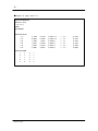
Software authors
◆ myPresto version 4
Nakamura, Haruki
Fukunishi, Yoshifumi
Eiji, Kanamori
Kubota, Satoru
Omagari, Katsumi
Fukuda, Ikuo
Wada, Mitsuhito
Mashimo, Tadaaki
Mitomo, Daisuke
◆ myPresto version 3
Nakamura, Haruki
Fukunishi, Yoshifumi
Jae Gil Kim
Watanabe, YS
Omagari, Katsumi
Mikami, Yoshiaki
Kubota, Satoru
Tatsumi,Rie
Horie, Masaru
Fukuda, Ikuo
◆ myPresto version 2
Nakamura, Haruki
Fukunishi, Yoshifumi
Jae Gil Kim
Mikami, Yoshiaki
Watanabe, YS
Ina, Yasuo
Horie, Masaru
Takahashi, Makoto
Fukuda, Ikuo
◆ myPresto version 1
cosgene version 1：
Nakamura, Haruki
Fukunishi, Yoshifumi
Hashi, Yuichi
Mikami, Yoshiaki
myPresto 4.2
v
Kidera, Akinori
Terada, Toru
tplgene version 1：
Nakamura, Haruki
Fukunishi, Yoshifumi
Kuroda, Masataka
Fukuda, Ikuo
myPresto 4.2
vi
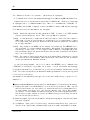
Cited references
Please refer to the following works when using this software.
myPresto and the filling potential method
1) "The filling potential method: A method for estimating the free energy surface
for protein-ligand docking", Yoshifumi Fukunishi, Yoshiaki Mikami, and Haruki
Nakamura, J. Phys. Chem. B. (2003) 107, 13201-13210.
cosgene multicanonical MD
2) "Determination of multicanonical weight based on a stochastic model of sampling
dynamics", Jae Gill Kim, Yoshifumi Fukunishi, Akinori Kidera and Haruki Nakamura,
Physical Review E (2003) 68, 021110.
3) "Multicanonical molecular dynamics algorithm employing adaptive force-biased
iteration scheme", Jae Gil Kim, Yoshifumi Fukunishi, Haruki Nakamura, Phys. Rev.
E 70, 057103 (2004).
Particle Mesh Ewald(PME)
4) U.Essmann, L.Perera, M.L.Berkowitz, T.Darden, H.Lee and L.G.Pedersen. A smooth
particle meth Ewald method.
J. Chem. Phys. 103, 8577-8593(1995)
Accessible surface area (ASA)について
5) Kinjo, A. R., Kidera, A., Nakamura, H. & Nishikawa, K. Physicochemical evaluation
of protein folds predicted by threading.
Eur Biophys J 30, 1-10. (2001).
Fast Multipole Method (FMM)
6) J. A. Board, Z. S. Hakura, W. D. Elliott, and W. T. Rankin. “Scalable variants
of multipole-accelerated algorithms for molecular dynamics applications”In
Proceedings of the Seventh SIAM Conference on Parallel Processing for Scientific
Computing, February 1995.
7) W. T. Rankin,“Efficient Parallel Implementations of Multipole Based N-Body
Algorithms.“PhD thesis, Duke University, Department of Electrical and Computer
Engineering, P.O.Box 90291, Durham, NC 27708-0291, April 1999.
8) W. T. Rankin, DPMTA ?Distributed Parallel Multipole Tree Algorithm, Duke University,
Durham, NC (2002).
sievgene
9) "Similarity among receptor pockets and among compounds: Analysis and application
to in silico ligand screening", Y. Fukunishi, Y. Mikami, and H. Nakamura, The Journal
of Molecular Graphics and Modelling 24 (2005) 34-45.
Multiple Target Screening (MTS) method
10) "Multiple target screening method for robust and accurate in silico screening",
Y. Fukunishi, Y. Mikami, S. Kubota, H. Nakamura, Journal of Molecular Graphics and
myPresto 4.2
vii
Modelling,25, 61-70 (2005).
11) "Noise reduction method for molecular interaction energy: application to in silico
drug screening and in silico target protein screening", Y. Fukunishi, S. Kubota,
H. Nakamura, Journal of Chemical Information and Modeling, 46, 2071-2084 (2006).
12) "Improvement of protein-compound docking scores by using amino-acid sequence
similarities of proteins", Y. Fukunishi, H. Nakamura, Journal of chemical
information and modeling, 48, 148-156 (2008)
Docking Score Index (DSI) method
13) "Classification of chemical compounds by protein-compound docking for use in
designing a focused library", Y. Fukunishi, Y. Mikami, K. Takedomi, M. Yamanouchi,
H. Shima, H. Nakamura, Journal of Medicinal Chemistry, 49, 523-533 (2006).
14) "An efficient in silico screening method based on the protein-compound affinity
matrix and its application to the design of a focused library for cytochrome P450
(CYP) ligands", Y. Fukunishi, S. Hojo, H.Nakamura, Journal of chemical information
and modeling, 46, 2610-22 (2006).
Maximum Volume Overlap (MVO) method
15) "Prediction of protein-ligand complex by docking software guided by other complex
structures", Y. Fukunishi, H. Nakamura, Journal of Molecular Graphics and Modelling,
26 (2008) 1030-1033.
Other references are listed at the end of this document.
myPresto 4.2
viii
ACKNOWLEDGEMENT:
This work was supported by grants from New Energy and Industrial Technology Development
Organization (NEDO) and Ministry of Economy, Trade and Industry (METI), JAPAN.
This software was developed as part of a research project advanced by the late Dr.
Yoshimasa Kyogoku.
The Particle Mesh Ewald (PME) routines were originally developed by Dr. Tom Darden [28].
National Institute of Environmental Health Sciences,
Research Triangle Park,
North Carolina 27709 US.
The Accessible Surface Area (ASA) routines were originally developed by Dr. Akira Kinjo [40].
Center for Information Biology and DNA Data Bank of Japan,
National Institute of Genetics,
Mishima, Shizuoka, 411-8540, Japan.
The Fast Multipole Method (FMM) routines were originally developed by Dr. William T. Rankin.
Center for Computational Science and Engineering
Duke University
Dept. of Electrical and Computer Engineering
Box 90291
Durham, NC 27708-0291 US.
myPresto 4.2
ix
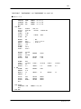
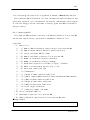
Table of Contents
1
2
Overview .............................................................. 1
1.1
Molecule dynamics simulation system: myPresto .............................. 1
1.2
Topology generator：tplgene ................................................ 2
1.3
Low molecule topology generator: tplgeneL .................................. 2
1.4
Conformation search engine: cosgene ........................................ 2
1.5
Installation................................................................ 3
1.6
Compound database：LigandBOX ............................................... 4
tplgene ............................................................... 7
2.1
Execution................................................................... 7
2.2
Creating input data........................................................ 10
2.2.1
3
4
PDB files............................................................ 10
2.3
Force field database file ................................................. 14
2.4
Environment variables...................................................... 15
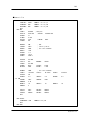
tplgeneL ............................................................. 16
3.1
Execution.................................................................. 16
3.2
Creating input data........................................................ 19
3.2.1
tplgeneL original format files ...................................... 19
3.2.2
Sybyl mol2 files..................................................... 21
3.3
Atom type definition file ................................................. 26
3.4
Force field parameter database file ....................................... 26
3.5
Fragment database file .................................................... 28
3.6
Environment variables...................................................... 29
cosgene .............................................................. 31
4.1
Execution.................................................................. 31
4.2
Input data creation........................................................ 31
4.2.1
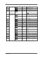
Control file......................................................... 31
4.2.1.1 EXE> INPUT
group................................................. 33
4.2.1.2 EXE> MINimize
group ............................................. 40
4.2.1.3 EXE> MD group..................................................... 58
4.2.1.4 EXE> OUTPUT group................................................. 81
4.2.1.5 EXE> END group.................................................... 82
myPresto 4.2
x
5
A
Sample calculations ................................................... 85
5.1
Sample-1：Peptide in a vacuum
- Calculation of Vassopressin - ............ 85
5.2
Sample-2: Protein in a vacuum
- Calculation of Lysozyme - ................ 88
5.3
Sample-3: Protein in water
5.4
Sample-4: Expanded ensemble（Force-biased McMD）−Calculation of Alanine peptide−102
5.5
Sample-5：Expanded ensemble (Simulated Tempering McMD) −Alanine peptide calculation−.. 106
5.6
Sample-6：Extend ensemble (Generalized ST McMD)−Calculation of Alanine peptide−110
5.7
Sample-7：Expanded sampling−Structure extraction and clustering ......... 117
5.8
Sample-8：Generation of low molecule topology
5.9
Sample-9：Free energy calculation（Filling Potential method）−Calculation of methane in water−125
5.10
Sample-10：RESPA method ................................................. 132
5.11
Sample-11：RATTLE
−Calculation of indometacin in water− .............. 134
5.12
Sample-12：Rigid
−Calculation of indometacin in water− ............... 137
5.13
Sample-13：Calculation of periodic systems using NPT and PME −Calculation of methane in water−140
5.14
Sample-14：Fast Multipole Method
5.15
Sample-15：GB/SA
- Calculation of Lysozyme - ................... 94
−Calculation of Methanol− 121
−MD calculation using counter ions− . 144
−Calculation of Vassopressin− ....................... 150
Input/Output files ....................................................155
A.1
Input/Output files of cosgene ............................................ 155
A.1.1
Explanation of phase ............................................... 155
A.2 Input Files................................................................ 156
A.2.1 Control file......................................................... 158
A.2.2 Topology files....................................................... 177
A.2.3 Coordinate file...................................................... 188
A.2.4 SHAKE file........................................................... 189
A.2.5 Fixed atom and free atom designation file ........................... 191
A.2.6 CAP designation file ................................................ 193
A.2.7 ExtendCAP designation file .......................................... 195
A.2.8 Position restraint file ............................................. 199
A.2.9 Distance restraint file ............................................. 201
A.2.10 Dihedral angle restraint file ...................................... 203
A.2.11 Monitor designation file ........................................... 205
A.2.12 File for designating center of mass alignment of system ............ 207
A.2.13 System GB/SA and ASA parameter specification file .................. 209
A.2.14 Umbrella restraint file ............................................ 211
A.2.15
myPresto 4.2
Restart file....................................................... 214
xi
A.2.16 Rigid body model file .............................................. 217
A.3 Output files............................................................... 219
A.3.1 MIN energy trajectory ............................................... 220
A.3.2 MD energy trajectory ................................................ 222
A.3.3 Monitor designation trajectory ...................................... 224
A.3.4 Total energy data.................................................... 226
A.3.5 Coordinate trajectory ............................................... 227
A.3.6 Velocity trajectory.................................................. 229
B
Utilities ............................................................231
B.1
setwater.................................................................. 231
B.2
mergetpl.................................................................. 233
B.3
SHAKEinp.................................................................. 235
B.4
RIGIDinp.................................................................. 236
B.5
GBSAinp................................................................... 238
B.6
Free energy calculation (Filling potential method + WHAM method) analysis 239
B.6.1
Generate_NextFP..................................................... 239
B.6.2
Extract_Atom........................................................ 241
B.6.3
Wham_Analysis....................................................... 242
B.7
Expanded ensemble analysis tools ......................................... 244
B.7.1
reweightFB.......................................................... 245
B.7.2
reweightST.......................................................... 246
B.7.3 reweightGST.......................................................... 248
B.7.4 selection............................................................ 249
B.7.5
B.8
clustering.......................................................... 251
Existing probability（Potential Mean Force）analysis tool ................ 256
B.8.1 pmf.................................................................. 256
B.8.2 contour.............................................................. 258
B.9
pca ....................................................................... 259
B.10
Gamess2tplinp............................................................ 261
B.11
Gauss2tplinp............................................................. 262
B.12
tpl2mol2................................................................. 263
B.13
add_ion.................................................................. 264
B.14
confgene................................................................. 266
B.15
confgeneC................................................................ 269
B.16
Free energy perturbative method (under development) ..................... 271
B.16.1 Calculation method.................................................. 271
myPresto 4.2
xii
B.16.2 vdw parameter and electrical charge scaling function（cosgene） .... 273
B.16.3 Analyze............................................................. 275
B.16.4 FEP................................................................. 277
B.17
Hgene.................................................................... 278
References ..............................................................279
myPresto 4.2
xiii
myPresto 4.2
1
1
Overview
1.1
Molecule dynamics simulation system: myPresto
myPresto is a molecule dynamics simulation system for biomolecules which i s equipped
with a conformation search engine based on a highly efficient conformation search
algorithm. myPresto was developed with the goal of creating an efficient general
purpose system for the simulation of three-dimensional dynamic biomolecule structures
and free energy calculation. The main areas of application include protein modeling,
protein - pharmaceutical low molecule modeling, pharmaceutical docking, and
calculation of film proteins.
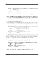
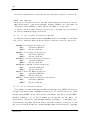
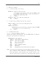
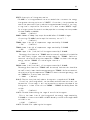
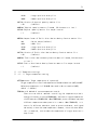
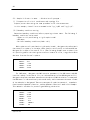
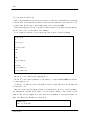
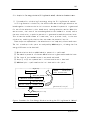
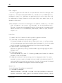
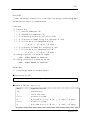
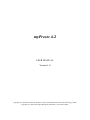
myPresto version 4.0 is composed of the subsystems indicated below. The procedure
for using the system is divided into the following stages: initial molecule
coordinates and topology file preparation (tplgene/tplgeneL), energy minimization
and MD calculation（cosgene）, and analysis of results using the analysis tools.
① Topology generator: tplgene
② Low molecule topology generator: tplgeneL
③ Conformation search engine：cosgene
④ Assembly of tools
⑤ Compound database：LigandBOX
Initial molecule coordinates and topology file preparation
（tplgene/tplgeneL）
Energy minimization and MD calculation
（cosgene）
Analysis of results using analysis tools
myPresto configuration
myPresto 4.2
2
1.2
Topology generator：tplgene
When performing energy minimization and MD calculation using myPresto, a topology
file must first be created for the molecule system. This file can be easily created
using the tplgene subsystem.
Using tplgene, even when incomplete Cartesian coordinates that are missing some
information (such as for a hydrogen atom) are used in standard input, complete
Cartesian coordinates can be obtained as an initial structure for performing the
conformation energy calculation. Supported force fields are AMBER and CHARMm.
1.3
Low molecule topology generator: tplgeneL
The low molecule topology generator tplgeneL can be used to create topology files
for ligands and other low molecules that are not supported by tplgene.
Supported force fields are AMBER parm99 and AMBER General Amber Force Field(GAFF).
Calculation of the MD of a high molecule - low molecule compound can be performed
by combining the topology files created with the tplgene and tplgeneL subsystems into
a single file.
1.4
Conformation search engine: cosgene
cosgene performs energy minimization and MD calculation using the initial molecular
coordinates and topology file that were prepared with tplgene as input. The main
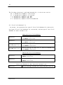
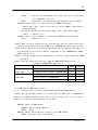
functions of cosgene are described below.
(Current version does not support the fast multipole method.)
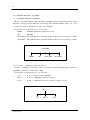
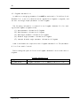
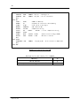
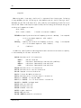
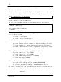
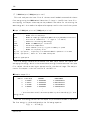
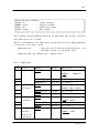
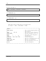
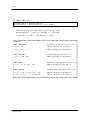
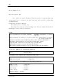
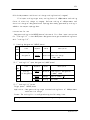
Main functions of cosgene
Function type
Description
Energy minimization
Steepest descent method, Steepest descent method with SHAKE,
Conjugate gradient method
MD calculation
Micro-Canonical, Canonical, Force-biased Multi-Canonical
Tsallis Dynamics（under development）
Integrator
Leap-frog (Verlet), Velocity Verlet, RESPA
Thermostat
Hoover-Evans Gaussian constraint, Nose-Hoover
Barostat
Andersen, Parrinello-Rahman
Long distance interaction
Direct summation, Direct summation & Cutoff,
Ewald, Particle Mesh Ewald, Fast Multipole Method
Restraint method
SHAKE, RATTLE, Rigid-body,
Position restraint, Distance restraint
Boundary conditions
Sphere, ellipsoid, periodic boundary conditions
※Shaded items in the above table are not supported in this release.
myPresto 4.2
3
1.5
Installation
（１）System requirements
・UNIX（Linux）environment ： Environment in which myPresto is run.
・C compiler
： Used to build tplgene and tplgeneL.
・Fortran90 compiler
： Used to build cosgene.
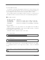
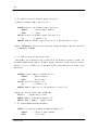
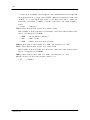
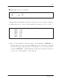
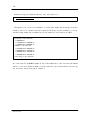
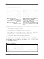
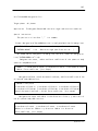
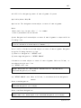
（２）Installation method
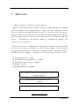
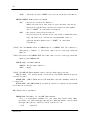
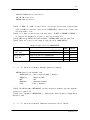
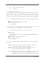
Copy the myPresto directory and its subdirectories to the desired installation
directory.
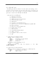
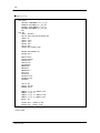
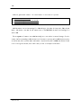
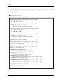
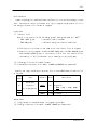
The myPresto directory consists of the following subdirectories:
・tplgene ：tplgene main module
・tplgeneL：tplgeneL main module
・cosgene ：cosgene main module
・tools
： Tool set
・doc
： Documentation
・sample
： Sample data （goes with chapter 5, "Calculation Examples", in this
manual）
myPresto
tplgene
bin DB src
tplgeneL
cosgene
bin DB src
bin src
tools
doc
sample
sample1
sample2 ...
sampleN
Use the "make" command in the "src" directory of tplgene, tplgeneL, and cosgene.
Compile the tools in "tools" as needed.
【Note】It may be necessary to modify Makefile to suit your compiler environment.
myPresto 4.2
4
1.6
Compound database：LigandBOX
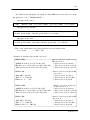
（１）Compound database LigandBOX
Mol2 file format dataset made by adding hydrogen atoms and estimating the total
molecular charge from the 2D electron catalog distributed by Namiki Shoji Co., Ltd.
in order to convert 2D molecular data into 3D data.
The directory configuration is as follows:
・MOLDB
：Compound database preparation tool
・doc
：Document
・mol2_2004 ：3D compound data prepared based on 2D electron catalog in 2004.
・mol2_2005 ：3D compound data prepared based on 2D electron catalog in 2005.
LigandBOX
MOLDB
doc
mol2_2004
mol2_2005
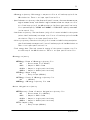
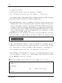
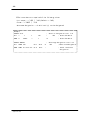
（２）Protein−compound interaction matrix
Protein − compound interaction matrix prepared from 3D compound data based on
LigandBOX
2D electron catalog in 2004.
The directory configuration is as follows:
・list
：List of proteins and compounds
・Matrix
：Protein−compound interaction matrix
・tools
：Protein−compound interaction matrix analysis tool
Matrix
list
myPresto 4.2
Matrix
tools
5
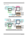
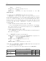
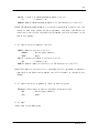
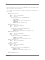
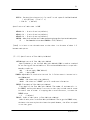
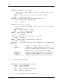
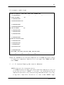
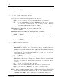
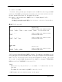
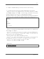
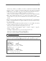
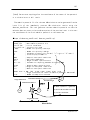
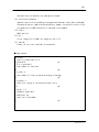
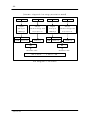
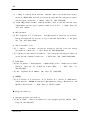
◆Execution examples
Protein information
Pocket search
PDB
or
residue list
Protein – Ligand
docking
Pocket
information
sievgene
Ligand
PDB
Conformer generation
tplgene
Global search
PDB
Topology generation
Local search
Hydrogen addition
Score evaluation
Topology
information
Scores,
RMSD etc.
Parameter
data base
Topology generation
Score analysis tool
Ligand information
evaluation
score result
Clustering
Clustering
result
low molecule
Data analysis
mol2
rough in silico screening ∼ tplgene & sievgene ∼
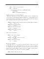
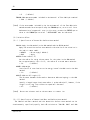
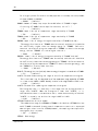
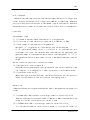
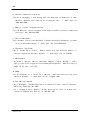
Protein information
Structural search（MD）Complex information
PDB
Complex
PDB
Topology
information
Merge
(complex information)
cosgene
MIN & MD
Topology
information
Force-bias McMD
GB/SA
Ligand information
Trajectory
・physical
quantities
Filling Potential
Ligand
PDB
GAMESS
tplgeneL
Topology
information
feedback
Topology generation
Quantum
calculation
result
(low molecule)
Analytical
data for FP
Parameter
data base
Topology generation
Analysis tools for FP
Analysis tools for McMD
Data analysis
Free energy
data
Canonical
distribution
data
Structural optimization and free energy calculation ∼ tplgeneL & cosgene ∼
myPresto 4.2
7
2 tplgene
2.1
Execution
tplgene creates initial coordinate and topology files for a molecule using data
related to the structure of the target molecule (PDB files and DIHED files) as input.
Directories referenced during calculation (directories for input files, output
files, and force field DB files) can be set in environment variables. If environment
variables will not be used, copy the input files and force field DB files to the
execution directory ahead of time, as the current directory will be used.
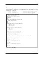
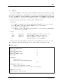
When tplgene is executed, the following items are specified. These items can be
entered interactively from the screen, or using command line options.
■Input items
・Title of topology file
・Molecule name
・Molecule type（1： Peptide chain, 2： DNA or RNA chain）
・Input file format（1：PDB, 2：DIHED）
・Force field DB file name
・Input file name
・Output PDB filename
・Output TPL filename
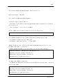
% tplgene
or
% tplgene （option）
Items specified using command line options are skipped during interactive input.
Only items that were not specified using command line options are entered
interactively.
myPresto 4.2
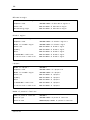
8
-title
<title_name>
Specify the title in <title_name>
-molname
<molculer_name>
Specify the molecule name in <molculer_name>
-i
<input_coord>
Specify the input coordinate file name in <input_coord>
-db
<db_file>
Specify the force field DB file name in <db_file>
-chain
[ pep ￨ nuc ]
Specify the type of molecule calculated
Peptide
⇒ pep
Nucleotide ⇒ nuc
-filetype [ pdb ￨ dihed ]
Specify the type of input file
PDB file format
⇒ pdb
DIHED file format ⇒ dihed
-outcrd
<output_coord>
Specify the output coordinate file name in <output_coord>
-outtpl
<output_tpl>
Specify the output topology file name in <output_tpl>
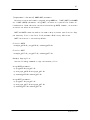
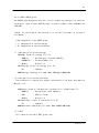
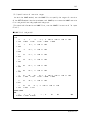
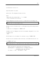
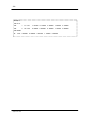
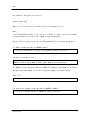
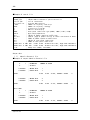
■Example of option specifications（underlined parts are entered）
% tplgene -i vas.dih -chain pep -filetype dihed -db C96_aa.tpl
Instructions for using tplgene can be viewed by specifying the option "-h" or
"-help".
% tplgene
-h
or
% tplgene
myPresto 4.2
-help
9
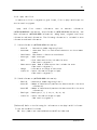
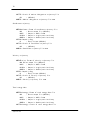
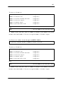
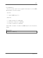
Items entered interactively (control specification) can be saved in a file
(control_file) to eliminate the trouble of entering the items each time tplgene is
executed.
% tplgene
<
control_file
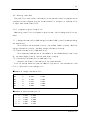
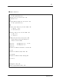
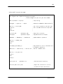
■Control file example
ALA-ALA
： Title line. Anything can be entered in 10 lines or less.
END
： Enter "END" at the end of the title lines.
ALA-ALA
： Molecule name. Any name can be entered
GLY-GLY
： To calculate multiple molecules, write each molecule name
on its own line.
END
： Enter "END" as the final line of the molecule names.
1
： Enter "1" for a peptide chain, or "2" for DNA or RNA.
1
： Enter "1" for PDB input, or "2" for DIHED input.
C96_aa.tpl
： Enter the force field DB file name.
ALA-ALA-input.pdb
： Enter the input file name.
ALA-ALA_out.pdb
： Enter the output PDB file name.
ALA-ALA-out.tpl
： Enter the output TPL file name.
The results output by tplgene are a topology that takes into account all atoms of
the molecule system, and coordinate information. These two sets of information can
be used to perform many conformation energy calculations.
If you wish to use separate directories for the data related to the structure of
the target molecule, the force field used, and the output files, each path can be
specified in an environment variable. If no environment variables are configured,
the current directory at the time of execution is used (refer to "2.2.4 Environment
Variables").
myPresto 4.2
10
2.2
2.2.1
Creating input data
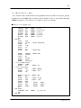
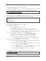
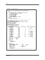
PDB files
Files in standard PDB format are used. The required information is indicated below.
(１) Amino acid residue name and residue sequence information
(２) Names of atoms of amino acid residues and cartesian coordinate information
(３) Disulfide bond information
(４) Circular molecule information
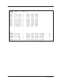
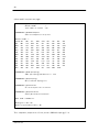
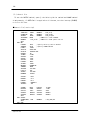
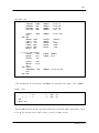
(1) and (2) above are required. (3) and (4) can be specified as necessary.
Disulfide bonds are defined according to normal PDB format. When calculating a
circular molecule, specify the keyword "CIRCLE" on the line prior to the ATOM lines
(see the example below).
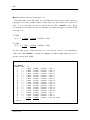
When information o n several molecules (several chains) is included in the PDB file,
calculations of all included molecules are performed.
If your system includes metal ions and water molecules, these atoms must be specified
by “HETATM” instead of “ATOM”in the PDB file.
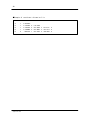
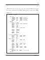
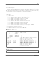
■Example of PDB file
myPresto 4.2
11
SSBOND
1 CYS A
6
CYS A
11
CIRCLE
ATOM
20
N
GLU A
4
33.037 -5.952
10.469
ATOM
21
CA
GLU A
4
33.629 -7.247
10.859
ATOM
22
C
GLU A
4
32.721 -7.845
11.909
ATOM
23
O
GLU A
4
32.470 -9.061
11.856
ATOM
24
CB
GLU A
4
35.029 -7.100
11.439
ATOM
25
CG
GLU A
4
36.081 -6.452
10.545
ATOM
26
CD
GLU A
4
35.906 -5.028
10.096
ATOM
27
OE1 GLU A
4
35.591 -4.102
10.842
ATOM
28
OE2 GLU A
4
36.158 -4.867
8.851
･
･
･
TER
HETATM
29 Zn
ZN
1
29.157
3.021
20.624
1.00 41.80
Zn
HETATM
30
Zn
ZN
2
20.538
16.287
4.630
1.00 43.88
Zn
HETATM
32
O
HOH
1
29.669
21.569
37.480
1.00 49.12
O
HETATM
33
O
HOH
2
20.132
6.585
18.359
1.00 60.57
O
HETATM
34
O
HOH
3
23.610
26.063
37.625
1.00 62.85
O
myPresto 4.2
12
2.2.2
DIHED files
If you wish to generate Cartesian coordinates for one molecule, an effective method
is to use a file in DIHED format. This format makes it possible to use the system
by providing only amino acid residue and disulfide bond information, together with
circular molecule information. The required information is indicated below.
(１) Amino acid residue name and residue sequence information
(２) Circular molecule information
(３) Disulfide bond information
(４) Dihedral angle information
(1) above is required. (2) through (4) can be specified as necessary.
If dihedral angle information is not specified, an elongated chain structure will
be generated. If dihedral angle information is specified, a chain structure will be
generated according to the provided values.
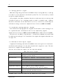
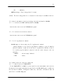
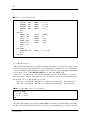
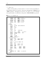
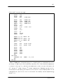
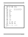
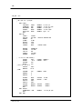
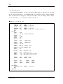
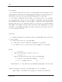
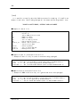
■Example of a DIHED file
The information entered in a DIHED file for a DODECA-PEPTIDE is as shown below.
This peptide chain consists of 12 residues, and there is a disulfide bond between
the 6th and 9th residues (CYS-CYS).
PRE>SEQUENCE
ASP
：1
LYS
：2
CYS
：3 -----+
CYS
：4
￨
HIS
：5
￨
HIS
：6
LEU
：7
￨
TRP
：8
￨
CYS
：9 -----+
GLN
：10
GLU
：11
GLU
：12
S-S BRIDGE
PRE>SSBONDS
3
9
For amino acid residues in the PDB, enter the keywords below. Entries are from
several groups beginning with "PRE>".
myPresto 4.2
13
（１）Amino acid sequence（PRE>SEQUENCE）
Describe the amino acid residue sequence.
Starting from the next line after
"PRE>SEQUENCE", enter amino acid names in succession from the N terminal side. Enter
one amino acid name per line.
Amino acids that can be used are as follows, for both the C96 and C99 data bases.
ACE （N terminal acetyl group）/ ALA / ARG / ASN / ASP / ASH (ASP neutral) / CYS /
CYSS / GLN / GLU / GLH (GLU neutral) /GLY / HIS / HISE / HIS / ILE / LEU / LYS / MET
/ PHE / PRO / SER / THR / TRP / TYR / VAL / NMEC (C terminal methyl group) / NHEC
(C terminal amino group)
/ ABA （2-aminobutanoic acid） / NLE (2-aminohexanoic acid) / SEP (SER phosphate)
/ TYP (TYR phosphate) / THP (THR phosphate) / LYN (LYS neutral) / CYM (S- non-protonated
CYS)
（２）Specification of a circular molecule（PRE>CIRCULAR）
This indicates that the molecule is circular.
（３）Specification of S-S bond（PRE>SSBOND）
If the molecule has a disulphide bond, specify the bond as shown below.
PRE>SSBOND
3
9
：1 st line. Indicates that the molecule has a disulfide bond.
：#3 and #9 residues are joined by the SS bond.
（４）Specification of dihedral angles（PRE>DIHEDRAL-ANGLES）
Enter dihedral angle information. Enter φ, ψ, ω, and χ from the N -terminal to
the C-terminal. Up to ten angles can be entered on each line. The angle definition
follows ECEPP.
The following processing is performed within the program;
‘+’；Added to the end of the group name when LYS, ARG, or HIS is protonated.
‘-' ；Added when ASP or GLU is non-protonated.
‘E’；Added if HIS has an AN HE hydrogen instead of an ANHD hydrogen.
‘S’；Added if CYS forms a disulphide bond.
The following processing is performed for N and C terminals.
‘N+’； Protonated N terminal
‘N ' ； Neutral N terminal
‘C-’； Non-protonated C terminal
‘C ’； Neutral C terminal
myPresto 4.2
14
The following processing is performed automatically in the current version.
'N+' is automatically added for an N terminal.
'C-' is automatically added for a C terminal.
'+' is automatically added for LYS, ARG.
'-' is automatically added for ASP, GLU.
'S' is automatically added to disulfide bonded CYS.
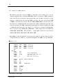
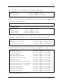
2.3
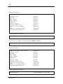
Force field database file
At present, the system has four types of force field databases for amino acids,
two types of force field databases for nucleotides, and one type of force field
dababase for water and metal ions.
Amino acid force field databases
Contains topology information for all amino acid monomers for
C96_aa.tpl
the AMBER96 force field.
Contains topology information for all amino acid monomers for
C99_aa.tpl
the AMBER96 force field.
charmm19_aa_all.tpl
charmm22_aa_all.tpl
Contains topology information for all amino acid monomers for
the CHARMm19 force field.
Contains topology information for all amino acid monomers for
the CHARMm22 force field.
Nucleotide force field databases
C96_na.tpl
C99_na.tpl
Contains topology information for all nucleotides for the
AMBER96 force field.
Contains topology information for all nucleotides for the
AMBER99 force field.
Force field database of water molecules and metal ions
metals.tpl
myPresto 4.2
Contains topology information for water molecules and ions.
15
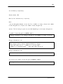
2.4
Environment variables
If you wish to calculate using separate directories for data relating to the
structure of the applicable molecule, the force field to be used, and the output file,
you can designate the path of each directory using environment variables.
The following 3 types of environment variables can be set. If you do not set
environment variables, the current directory will be accessed during execution.
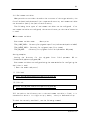
■Environment variables
Environment variable name
TPL_INPUT_PATH
TPL_OUTPUT_PATH
TPL_DB_PATH
Explanation
：Directory for tplgene input file (Must include path)
：Directory for tplgene output file (Must include path)
：Directory for tplgene force field DB (Must include path)
(Setting example)
Suppose you wish to set the directory for the tplgene force field DB to
"/home/user01/myPresto/tplgene/DB". To set the environment variables, follow the
setting method of the shell you are using.
(The underlined part indicates the part to be input.)
（１）In case of bash
% export TPL_DB_PATH=/home/user01/myPresto/tplgene/DB
（２）In case of csh
% setenv TPL_DB_PATH /home/user01/myPresto/tplgene/DB
※If the path to the directory (set in the environment variable) will not change,
it is convenient to write it into a login script (.bashrc, .cshrc) or a dedicated
script.
The shell which is currently being used can be checked using the following command.
% ps
myPresto 4.2
16
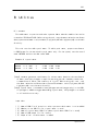
3
tplgeneL
3.1
Execution
Using data (tplgeneL original format files or mol2 files) on the structure of the
target molecule as input, tplgeneL creates initial coordinate and topology files for
the molecule.
Directories (for input files, output files, and force field DB files) accessed
during calculation can be set in environment variables. If environment variables are
not configured, the current directory is used, and thus the input files, atom type
definition files, and force field parameter DB files must be copied to the execution
directory prior to execution.
When executing tplgeneL, specify the following items. These items can be entered
interactively from the screen, or specified using command line options.
■Items entered
・Input file format（1：tplgeneL original format, 2：Sybyl mol2 format）
・Input file name
・Processing method when parameters are missing.
(1： Use default parameters, 2： Automatically calculate parameters,
3：Use default parameters. Dynamically calculate parameters for items with no
parameters. )
・Parameter DB file name
・Use fragment DB? (yes: use, no: do not use)
% tplgeneL
or
% tplgeneL （option）
When an item is specified using a command line option, input of that item by
interactive entry is skipped. Only items that are not specified using command line
options are entered interactively.
myPresto 4.2
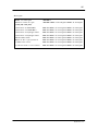
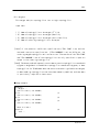
17
-ft
[ 1 ￨ 2 ]
Specify the input file format.
tplgeneL original input file
Sybyl mol2 input file
-i
： 1
： 2
<file>
Specify the input file name in <file>
-d
<db_file>
Specify the parameter DB file name in <db_file>.
-r
<resname>
Specify the residue name to be indicated in the output topology file in
<resname> (4 characters or less).
-f
[ yes ￨ no ]
Specify whether or not the fragment DB is used.
Use
⇒
Do not use
-p
yes
⇒
or y
no or n
[ 1 ￨ 2 ]
Select the method for compensating for missing parameters
Default parameters
Dynamic compensation
：
1
：
2
Default parameters ＋ dynamic compensation
：
3
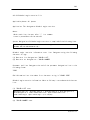
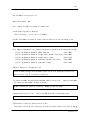
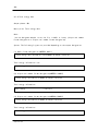
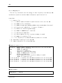
■Example of specifying options（underlined parts are entered）
% tplgeneL -i methanol -d prm_gaff.db -f no
The option "-h" or "-help" can be specified to view the instructions for using
tplgene.
% tplgeneL
-h
or
% tplgeneL
-help
myPresto 4.2
18
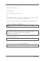
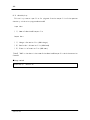
Interactive input (control) items can be stored in a file (control file) to eliminate
the trouble of having to enter the items interactively each time tplgeneL is executed.
% tplgeneL
<
control_file
■Control file example
1
methanol
1
prm_gaff.db
no
：Input file format (1:original、2:mol2)。
：File name (omit the extension).
：Compensation method for missing parameters
：(1: default, 2: dynamic compensation).
：Parameter DB file name
：Indicate whether or not fragment DB is used (yes/no)。
The high molecule topology file obtained with tplgene and the topology file obtained
with tplgeneL can be combined to perform MD simulation of the high molecule - low
molecule complex using cosgene.
If you wish to use separate directories for the target molecule structure data,
the force field used, and the output files, the paths of the directories can be
specified in environment variables. When environment variables are not configured,
the current directory at the time of execution is used (refer to "3.2.6 Environment
variables").
myPresto 4.2
19
3.2
Creating input data
The input files that contain information on the molecule used in tplgeneL can be
created in either tplgeneL original format (bond file, charge file, and zmat file)
or Sybyl mol2 format (mol2 file).
3.2.1
tplgeneL original format files
When using input files in tplgeneL original format, the following three files are
used:
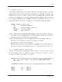
（１） Charge information file (XXX.charge file (where "XXX" is the file name excluding
the extension)).
This contains the atom name (item 1), the element symbol (item 2), Mulliken
charge information (item 3), and Resp charge information (item 4).
（２）Bond information file (XXX.bond file)
This shows the combinations of the numbers of the bonded atoms (items 1 and
2), the bond length (item 3), and the bond order (item 4).
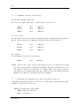
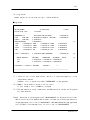
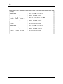
（３）Coordinate information file (XXX.zmat file)
Contains the Z-matrix information of the input molecule.
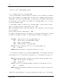
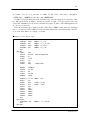
Files (1) and (2) above are required. When file (3) exists, the information in the
file is reflected in the topology file.
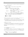
■Example of charge information file
C1
C
-0.1320
-0.1320
O2
O
-0.7323
-0.7323
H3
H
0.1340
0.1340
H4
H
0.1653
0.1653
H5
H
0.1644
0.1644
H6
H
0.4006
0.4006
■Example of bond information file
1
2
1.4130
0.7600
1
3
1.1160
0.9530
1
4
1.1200
0.9480
1
5
1.1200
0.9480
2
6
0.9630
0.7970
myPresto 4.2
20
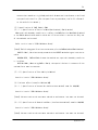
■Example of coordinate information file
C
O
1
1.4132350
H
1
1.1159340
2
112.6746
H
1
1.1195330
2
107.3658
3
121.0117
0
H
1
1.1196880
2
107.4483
3 -121.0171
0
H
2
.9627370
1
107.7002
5 -120.0241
0
myPresto 4.2
21
3.2.2
Sybyl mol2 files
In addition to files in tplgeneL original format, files in Sybyl mol2 format can
also be used in tplgeneL.
Sybyl
mol2
files
contain
information
such
as
molecule
information
(@<TRIPOS>MOLECULE information), atom information (@<TRIPOS>ATOM information), and
bond information (@<TRIPOS>BOND information). Among these, tplgeneL uses atom
information and bond information. The following information is included in atom
information and bond information.
（１）Atom information (@<TRIPOS>ATOM information)
・Atom ID
・Atom name
： Consecutive number beginning from 1.
： Atom name. The first and second characters are the element
symbol.
・Coordinates： Coordinates in Cartesian coordinates.
・Atom type ：Sybyl atom type.
・SuID
：ID of substructure that includes the atom.
＜Not used in tplgeneL.＞
・Substructure name： Name of substructure that includes the atom.
＜Not used in tplgeneL.＞
・Charge
：Information on charge of each atom.
・status bit ：Status information unique to Sybyl.
＜Not used in tplgeneL.＞
（２）Bond information (@<TRIPOS>BOND information)
・Bond ID
：Consecutive number beginning from 1.
・Atom ID１ ：Number of bound atom 1 (matches the above atom ID in the atom
information).
・Atom ID２ ：Number of bound atom 2 (matches the above atom ID in the atom
information).
・Bond type ：Bond type (1, 2, 3, am, ar, du, un, nc).
・status bit ：Status information unique to Sybyl.
＜Not used in tplgeneL.＞
【Reference】Refer to the following for information on the Sybyl mol2 file format:
Tripos Online Mol2 File Format
URL
http://www.tripos.com/custResources/mol2Files/index.html
myPresto 4.2
22
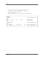
■Example of Sybyl mol2 file
@<TRIPOS>MOLECULE
methanol.mol2
6 5 0 0 0
SMALL
NO_CHARGES
@<TRIPOS>ATOM
1 C
0.7253
0.0134
0.0001 C.3
1
<1>
-0.1320
2 O
-0.6859
-0.0645
-0.0000 O.3
1
<1>
-0.7323
3 H
1.0981
1.0651
0.0186 H
1
<1>
0.1340
4 H
1.0901
-0.5342
0.9059 H
1
<1>
0.1653
5 H
1.0900
-0.5012
-0.9251 H
1
<1>
0.1644
6 H
-1.0287
0.8351
0.0005 H
1
<1>
0.4006
@<TRIPOS>BOND
1
1
2
1
2
1
3
1
3
1
4
1
4
1
5
1
5
2
6
1
myPresto 4.2
23
【Supplemental information】Reading mol2 files into tplgeneL
・Mol2 file information referenced by tplgeneL
tplgeneL does not reference @<TRIPOS>MOLECULE information.
Only atom and bond information
@<TRIPOS>ATOM
：
@<TRIPOS>BOND
：
in the specified mol2 file is obtained and processed. For this reason,
・If there is a format error in the ATOM or BOND sections, tplgeneL will show
and error message and end.
・If there is a format error in @<TRIPOS> of other than ATOM or BOND, processing
will continue.
・Handling the status bit in the ATOM and BOND sections
The status bits in MOL2 files are specified internally by SYBYL.
The effective status bits are shown below. However, these items are not set by
the user, and thus tplgeneL does not perform an error check on these items.
（Reference） Effective status bits for ATOM
DSPMOD, TYPECOL, CAP, BACKBONE, DICT, ESSENTIAL, WATER, DIRECT
（Reference） Effective status bits for BOND
TYPECOL, GROUP, CAP, BACKBONE, DICT, INTERRES
・Handling bond types
The following bond types are defined in MOL2 files.
1 = single
2 = double
3 = triple
am = amide
ar = aromatic
du = dummy
un = unknown
nc = not connected
When the bond type "am" is specified, the bond is processed internally as a
single bond in tplgeneL. When the type "ar" is specified, it is processed as
an aromatic bond.
When the type "du", "un", or "nc" is specified, processing is not possible
in tplgeneL. An error message is output and the program ends.
myPresto 4.2
24
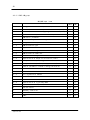
【Error messages and causes】
No.
1.
2.
Error message
ERROR> ltgReadMOParmMol2
Contents Error : filename.mol2
Start of next line must not begin with "@" or "#",
if line is continued with a back slash "¥".
Please check following information.
(data in vicinity of error)
ERROR> ltgReadMOParmMol2
Contents Error : filename.mol2
It is necessary to describe sign "@" and "#" in column
1 of the line.
Please check following information.
(data in vicinity of error)
ERROR> ltgReadMOParmMol2
Contents Error : filename.mol
Atom format is wrong.
Please check following information.
(data in vicinity of error)
3.
or
ERROR> ltgReadMOParmMol2
Contents Error : filename.mol
Bond format is wrong.
Please check following information.
(data in vicinity of error)
4.
Cause
The first character of a line following the
continue symbol is ”@” or ”#”.
"@" or "#" is in a position other than the
beginning of the line.
With respect to the ATOM section,
data continues after the continue symbol.
1st item includes characters other than numbers
(atom ID).
First character of 2nd item (atom name) is a
number.
3rd item (x coordinates) includes characters
other than numbers, "-", or "."
4th item (y coordinates) includes characters
other than numbers, "-", or "."
5th item (z coordinates) includes characters
other than numbers, "-", or "."
First character of 6th item (atom type) is a
number.
7th item (substructure ID) includes characters
other than numbers.
9th item (atom type) includes characters other
than numbers.
Less than 6 items or more than 10 items are
entered.
With respect to the BOND section,
data continues after the continue symbol.
1st item (bond ID) includes a character string.
2nd item (atom ID) includes a character string.
3rd item (atom ID) includes a character string.
Less than 4items or more than 5 items are
entered.
ERROR> ltgReadMOParmMol2
The 4th item (bond type) of the BOND section
Contents Error!
specifies a character string not defined in the
The Bondtype ( "bond type") that Mol2 Format does not MOL2 file format.
support is found.
Please check following information.
(data in vicinity of error)
myPresto 4.2
25
No.
Error message
ERROR> ltgReadMOParmMol2
Contents Error!
The Bondtype ("bond type") that tplgeneL does not
5.
support is found.
Please check and modify following information.
(data in vicinity of error)
ERROR> ltgReadMOParmMol2
6.
File Format Error : *.mol2
File Format is not correct.
ERROR> ltgDefineBond
Contents Error!
7.
Isolated Atom ("atom name") that it has not any Bond
is detected in Input File.
Please check Input Files. : *.bond or *.mol2.
ERROR> ltgReadMOParmMol2
Contents Error!
8.
Bond information does not match to Atom information.
Please check mol2 file "filename.mol2 ".
ERROR> ltgDefineBond
Contents Error!
9.
The Bond Information is overlapped. : (Duplicate
atom combinations)
Please confirm Input Files. : *.bond or *.mol2.
Cause
The 4th item (bond type) of the BOND section is
defined in the MOL2 file format, however, a bond
type not supported by tplgene (du, un, or nc) is
specified.
No ATOM line or no BOND line.
ATOM items and BOND items do not correspond.
Too many ATOM items.
ATOM items and BOND items do not correspond.
Too many BOND items.
The same atom combination is entered more than
once in the BOND section.
myPresto 4.2
26
3.3
Atom type definition file
tplgeneL first assigns the atom type of each atom in the molecule to be calculated,
and then assigns force field parameters corresponding to each combination of atom
types.
The atom type definition file contains atom type information corresponding to the
environment (element symbol, number of bonds of atom, bond order, whether or not atom
is in a ring, aromatic or not) of each atom.
Atom type definition files for the following two types of force fields are available
in tplgeneL.
Atom type definition file
atomtype_gaff.db
atomtype_amber99.db
3.4
DB file of atom type assignment rules for AMBER GAFF force
fields
DB file of atom type assignment rules for AMBER parm99 force
fields
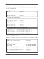
Force field parameter database file
tplgeneL assigns force field parameters based on the atom type assigned in "3.2.3
Atom type definition file".
The force field parameter database consists of the "prm_XXXX.db" file, which
contains bond parameters for each atom type, bond angle parameters, dyhedral angle
parameters, and improper dihedral parameter information, and the "nonbond_XXXX.db"
file, which contains function parameters and nonbond parameters.
Force field parameter database files are currently available for AMBER parm99 and
AMBER GAFF.
Force field parameter database files
prm_gaff.db
prm_amber99.db
nonbond_gaff.db
nonbond_amber99.db
myPresto 4.2
DB
DB
DB
DB
file
file
file
file
for
for
for
for
AMBER
AMBER
AMBER
AMBER
GAFF force field parameters
parm99 force field parameters
GAFF force field nonbond parameters
parm99 force field nonbond parameters
27
【Supplemental information】AMBER GAFF parameters
Calculation can be performed in tplgeneL using AMBER ver. 7 GAFF (GAFF7) and AMBER
ver. 8 GAFF (GAFF8) parameters. Using GAFF7, calculation is possible for almost all
low molecules. Fewer molecules can be calculated using GAFF8, however, an accurate
structure can often be calculated.
GAFF7 and GAFF8 cannot be used at the same time by a present specification. Copy
the necessary files in the force field parameter DB directory before use.
GAFF7 calculation is selected by default.
Files for GAFF8
atomtype_gaff8.db, prm_gaff8.db, nonbond_gaff8.db
Files for GAFF7
atomtype_gaff7.db, prm_gaff7.db, nonbond_gaff7.db
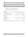
Example) Copying files
Use the following commands to copy the necessary files.
Using GAFF8 parameters
cp prm_gaff8.db prm_gaff.db
cp atom_type_gaff8.db atom_type_gaff.db
cp nonbond_gaff8.db nonbond_gaff.db
Using GAFF7 parameters
cp prm_gaff7.db prm_gaff.db
cp atom_type_gaff7.db atom_type_gaff.db
cp nonbond_gaff7.db nonbond_gaff.db
myPresto 4.2
28
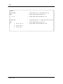
3.5
Fragment database file
In addition to assigning parameters from AMBER as explained in "3.2.4 Force field
database file", a part of a molecule can be regarded as a fragment in tplgeneL, and
the user can assign unique parameters to that fragment.
The following information is entered in the fragment database file for each
registered fragment (fragment block).
(１) Atom parameter information of fragment
(２) Bond parameter information of fragment
(３) Bond angle parameter information of fragment
(４) Dihedral angle parameter information of fragment
(５) Improper dihedral angle parameter information of fragment
Items 1 and 2 above are required to use a fragment database file. The parameters
of 3 to 5 are used if stored.
The following two types of force field fragment database files are available in
tplgeneL.
Fragment database files
frg_gaff.db
Fragment database file for AMBER GAFF force fields
frg_amber99.db
Fragment database file for AMBER parm99 force fields
myPresto 4.2
29
3.6
Environment variables
When you wish to store data related to the structure of the target molecule, the
force field used, and the output files in separate directories, environment variables
can be used to specify the path of each directory.
The following three types of environment variables can be configured. If no
environment variables are configured, the current directory at the time of execution
is used.
■Environment variables
Environment variable name
Description
TPLL_INPUT_PATH ： Directory for tplgeneL input files (indicate with path included）
TPLL_OUTPUT_PATH ： Directory for tplgeneL input files (same)
TPLL_DB_PATH
：Directory for tplgeneL force field parameters DB (same)
Setting examples
Setting
the
directory
for
the
tplgeneL
force
field
parameter
DB
to
"/home/user01/myPresto/tplgeneL/DB":
Environment variables are configured using the same method as for configuring the
shell that is used.
（Enter the underlined parts.）
（１）For bash
% export TPLL_DB_PATH=/home/user01/myPresto/tplgeneL/DB
（２）For csh
% setenv TPLL_DB_PATH /home/user01/myPresto/tplgeneL/DB
※If the path to the directory set in the environment variable is fixed, it is
convenient to write it in a login script (.bashrc, .cshrc) or dedicated script.
To check the currently used shell, use the following command.
% ps
myPresto 4.2
30
(Blank)
myPresto 4.2
31
4 cosgene
4.1
Execution
cosgene performs system energy minimization and MD calculation using information
on the target molecule such as the initial coordinates and topology file prepared
with tplgene and tplgeneL. The results of the calculations can be analyzed using the
analysis tools.
Molecular information such as the initial coordinates, topology file, and
calculation conditions are specified in the control file. cosgene loads the file by
standard input.
% cosgene
4.2
<
control_file
> output
Input data creation
4.2.1
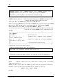
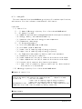
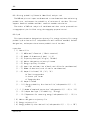
Control file
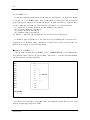
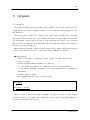
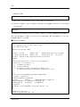
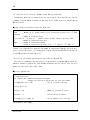
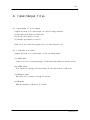
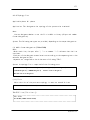
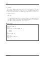
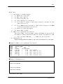
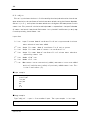
The control file consists of the following groups. Each group is ended with "QUIT".
・EXE> INPUT group
：Specifies the main input file names.
・EXE> MINI group
：Specifies options for energy minimization.
・EXE> MD group ：Specifies options for MD.
・EXE> OUTPUT group
：Specifies output of the final results.
・EXE> END
：Indicates the end of the control file.
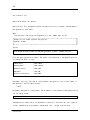
EXE> INPUT
TOPOLOGY= FORM
COORDINA= PDB
NAMETO= thrp.tpl
NAMECO= thrp.pdb
；Topology file
；Initial coordinates
QUIT
EXE> MINI
METHOD=
CONJ
；Energy minimization using t he c onjugate gradient method
LOOPLI=
40
UPDATE=
20
CUTMET=
DIEFUN=
RESA
DIST
CUTLEN= 8.0D0
DIEVAL= 2.0D0
；Calculate 40 times, update interaction table every 20 times.
；Set CUTOFF length for interaction to 8A
；Use distance-dependant dielectric constant
QUIT
EXE> OUTPUT
COORDINATE= PDB
NAMECO=
thrp_mini.pdb
；Final structure in PDB format
QUIT
EXE> END
Example of control file for energy minimization
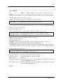
myPresto 4.2
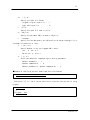
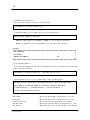
32
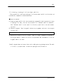
EXE> INPUT
TOPOLOGY=
COORDINA=
FORM
NAMETO=
serp.tpl
；Topology file
PDB
NAMECO=
serp.pdb
；Initial coordinates
QUIT
EXE> MD
LOOPLI=
20000
；Number of MD steps
UPDATE=
TIMEST=
20
0.5D0
；Frequency of interaction table updating
；Time step of time integral
METHOD=
CANONICAL
；NVT canonical MD
SETTEM=
INITIA=
300.0D0
；Temperature setting
SET
STARTT=
300.0D0 ； Initial temperature setting
RANDOM=
654321
CUTMET=
DIEFUN=
RESA
CONS
CUTLEN=
DIEVAL=
PDB
NAMECO=
10.0D0
1.0D0
；Specification of energy CUTOFF
；Dielectric constant
QUIT
EXE> OUTPUT
COORDINATE=
serp_md_1p.pdb
；Final structure in PDB format
QUIT
EXE> END
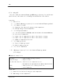
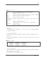
Example of control file for MD
Explanation of each control file command
Mandatory
◎
Can be omitted
△
Mandatory when the user designates certain functions
○
myPresto 4.2
33
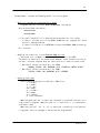
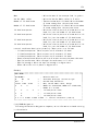
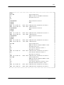
4.2.1.1 EXE> INPUT
group
The INPUT group specifies external files that specify the topology, initial
coordinates, and various atoms to be restrained or monitored (for the format of the
external files, refer to "A File Formats" at the end of the manual). The same input
group input is used for both "EXE> MIN" and "EXE> MD".
Items specified in the INPUT group：
（１）Topology of the system
（２）Coordinates of the system
（３）SHAKE atoms and restraining distance
（４）Fixed atoms and free atoms
（５）CAP potential
（６）Assignment of extended CAP potential
（７）Specifications for calculation of RMSD（when using MIN or MD）
（８）Position restraint
（９）Restraint of distance between atoms
（１０）Dihedral angle restraint
（１１）Monitored items
（１２）System GB/SA and ASA parameters
（１３）Umbrella restraint
（１４）Alignment of center of mass of system
（１５）QUIT
（１）Specification of topology of system
TOPOLOgy：Format of topology file（◎）
=NOREad
=FORMAtted
=BINAry
；No topology file input（default）
；Formatted ASCII file
；Binary file
UNITTOpology：IO units of topology file（△）
=10
；（default）
NAMETOpology=(Topology
file
name,
80
characters
or
less.
When
TOPOLOgy=[FORM￨BINA])
（２）Specification of system coordinates
COORDInate: Format of 3-dimensional coordinate file in PDB format（◎）
=NOREad
；No coordinate input (default)
=PDB
；PDB file format
myPresto 4.2
34
=BINAry
；Binary file
UNITCOordiante：IO units of coordinate file（△）
=11
；（default）
NAMECOordinate = (Coordinate file name, 80 characters
or
less.
When
COORD=[PDB￨BINA])
（３）Specification of SHAKE/RATTLE atoms and restraint distance
If SHAKE/RATTLE is used, the atomic number of the target atom and the restraint
distance may be designated by a file or the information may be automatically prepared.
In this file, in addition to regular restraint of distance between two atoms, special
distance restraint can also be specified in a 3-atom triangle (CH2 , H2 O) or 4-atom
tetrahedron (CH3 , NH3 ) topology.
SHAKE/RATTLE is automatically prepared by the
following method:
（a）Other than water molecule（molecule name is not "WAT"）
If one to three hydrogen atoms bind covalently to an atom that is not hydrogen,
their atomic distances are calculated and respectively set as SHAKE/RATTLE
information of two to four atoms.
（b）Water molecule（molecule name is "WAT"）
Set as SHAKE/RATTLE information of three atoms based on the bond distances of
water held in the program.
（３−１）SHAKE/RATTLE information input designation
SETSHAke：Read file specifying atoms to which SHAKE/RATTLE will be applied.（○）
=NOREad
；Do not use SHAKE/RATTLE (default)
=READ
；Use SHAKE/RATTLE
UNITSHake: IO Units of SHAKE specification file（△）
=12
；（default）
NAMESHake=(SHAKE file name, 80 characters or less (○))
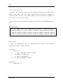
【Note】When using SHAKE/RATTLE, "SHAKEMethod= [HBON ￨ ALLB]" must also be specified
in the EXE> MD or EXE> MIN group.
【Note】There are limitations on the range of application of SHAKE/RATTLE.
Range of application of SHAKE/RATTLE
SHAKE
RATTLE
Energy minimization
Steepest gradient method （METHOD=STEEP） ○
×
（EXE> MIN）
Conjugate gradient method （METHOD=CONJ） ×
×
MD calculation
Leap Frog Verlet（INTEGR=LEAP）
×
myPresto 4.2
○
35
（EXE> MD）
Velocity-Verlet （INTEGR=VELO）
×
○
Multi Time Step （INTEGR=MTS）
×
×
（３−２）SHAKE/RATTLE automatic preparation information output designation
If SHAKE/RATTLE information is automatically prepared, the prepared information can
be output as a file. The format of the output file is the same as the input file.
DBGSHA：SHAKE/RATTLE automatic preparation information output designation（△）
=NOWRite ：Do not output file (default）.
=ASCIi
：Output file.
UNITDS：IO units of SHAKE/RATTLE automatic prepration information file（△）
=84
：（default）
NAMEDS = (SHAKE/RATTLE automatic preparation information file name, 133
characters or less)
（４）Specification of fixed atoms and free atoms
Atoms specified as fixed atoms are not subject to MIN/MD calculation, and are treated
as points where a force field is applied. Free atoms are subject to the normal MIN/MD
calculation. Atoms to be fixed can be specified by atom number, or by specifying a
particular center and radii R1 and R2 such that atoms at a distance R from the center
where R1 < R < R2 are specified. For this purpose, a control file is necessary. Free
atoms are specified in the same way. If these specifications are not made, all atoms
in the system are treated as free atoms.
SETVARiables=:Format of fixed/free atom designation file（△）
=NOREad ；No fixed atom designation (Default)
=READ
；Designate fixed atoms
UNITVAribles：IO unit of fixed atom designation file（△）
=13
；(Default)
NAMEVAriables =(Name of file designating fixed atoms, 80 chars. max.)
（５）Designation of CAP potential
This designates the atoms to which CAP potential is applied, coordinates of the CAP center,
and constants for radius and force. You can designate atoms in the CAP designation file, and
information like center coordinates can be designated either in the CAP designation file, or
in the control file. However, control file input will take priority.
myPresto 4.2
36
SETBOUndary：Designates atoms for applying CAP potential, and CAP radius and force
constants（○）
=NOREad
；Do not use CAP
=READ
；Use CAP
UNITBOundary：IO unit of CAP designation file（△）
=14
；(Default)
NAMEBOundary=(Name of CAP designation file, 80 chars. max.（○）)
【Note】 In EXE>MD, you must add "CALCAP=CALC", and also add the designation of CAP parameters.
It is best to designate "STOPCE=[TRANIBOTH]" and fix the 1st chain of the system (start
molecule) in space, so that CAP potential does not shift from the 1st chain.
（６）Designation of ExtendCAP potential
Specify atoms to which an ExtendCAP potential, restraint range, and force constant
are applied. A spherical or ellipsoidal body can be designated for the restraint range.
SETEXtendCap：Specify atoms to which an ExtendCAP potential, restraint range,
and force coefficient are applied.（○）
=NOREad
；ExtendCAP is not used. （default）
=READ
；ExtendCAP is used.
UNITExtendCap：IO Units of ExtendCAP designation file（△）
=23
；（default）
NAMEExtendCap=(ExtendCAP designation file name, 133 characters or less（○）)
【Note】"EXTCAP=CALC" should be added to EXE> MD. It is desirable to prevent the CAP
potential from deviating from the first chain by specifying "STOPCE= [TRAN￨BOTH]"
and spacially fixing the first chain (leading molecule) of the system.
（７）Designation for RMSD calculation (when using MIN or MD)
REFCOOrdinate：Reference file. The coordinate file in PDB format which serves as the basis.
=NOREad
; Do not use (Default)
=PDB
; Use
UNITREfcoordi：IO unit of reference file（△）
=15
; (Default)
NAMEREFcoordi=(Reference file name, 80 chars. max.)
【Note】 Add "BESTFIt=YES" to EXE>MD or EXE>MIN for RMSD calculation.
myPresto 4.2
37
（８）Designation of position restraint
You must prepare the following two files in order to use position restraint.
・A restraint designation file which designates the atoms to be restrained and
information about the force constant
・Reference file in PDB format listing coordinates to be restrained
REFCOOrdinate：Reference file, same as for RMSD（○）
=NOREad
；Do not use (Default)
=PDB
；Use
UNITREfcoordi：IO Unit of reference file（△）
=15
；Default
NAMEREFcoordi=(Reference file name, 80 chars. max.（○）)
POSITIonrestrain：Designation of applicable atoms and force constant etc.（○）
=NOREad
；Do not use (Default)
=READ
；Use
UNITPOsition：IO unit of file designating atoms to be constrained
=16
；（Default）（△）
NAMEPOsition=(Name of file designating atoms to be constrained, 80 chars. max. (○))
【Note】 You must also designate "CALPSR=CALC" and position restraint parameters in
EXE>MIN or EXE>MD.
（９）Designation of restraint distance between atoms
Prepare a file designating the distance restraint between atoms.
DISTANcerestrain：Use restraint distance between atoms
=NOREad
；Do not apply (Default)
=READ
；Apply
UNITDIstance：IO unit of distance designation file
=17
；(Default)（△）
NAMEDIstance=(Name of file for designating distance between atoms, 80 chars. max.)
【Note】 You must designate "CALDSR=CALC" and restraint potential weight parameters
in EXE>MIN or EXE>MD.
myPresto 4.2
38
（１０）Specification of dihedral angle restraints
Prepare a dihedral angle restraint file.
DIHEDRalrestrain：Use dihedral angle restraints
=NOREad
； Do not apply（default）
=READ
； Apply
UNITDH：IO units of dihedral angle restraint file.
=18
；（default）（△）
NAMEDH=（Name of dihedral angle restraint file, 80 characters or less）
【Note】"CALDHR=CALC" and restraint potential weight parameters must be specified
in EXE>MIN or EXE>MD.
（１１）Specification of monitored items
During MD, real-time monitoring is possible of coordinates of specific atoms, the
distance between atoms, angles, dihedral angles, and other items, with the results
output to a file. Prepare a file designating the atoms and pairs of atoms to be
monitored.
OUTMONitoritems： Monitor information file
=NOREad
；Apply（default）
=READ
；Do not apply
UNITMO：IO units of monitor file
=19
；（default）（△）
NAMEMO=（Name of monitor file, 80 characters or less（○））
【Note】Set the following items in EXE> MD.
OUTTRJ= n
： Output every n steps.
NAMETR= (Monitor information output file)
MNTRTR= [ASCI ￨ BINAry]
：Output format
（１２）System GB/SA and ASA parameters
ASAREA：File specifying GB/SA and ASA parameters（○）
=NOREad
； No file input（default）
=READ
； File input
myPresto 4.2
39
UNITSA： I/O units of GB/SA and ASA parameter file（△）
=77
；（default）（△）
NAMESA=（Name of GB/SA and ASA parameter file, 80 characters or less（○））
【Note】The GB/SA and ASA parameter file can be created using a special tool. The
radius of each atom, atomic solvation parameter, and other information are
specified in the file (for the specification method, see "A File Formats" at the
end of this manual).
（１３）Specification of umbrella restraint
UMBREL：Umbrella restraint file（○）
=NOREad
；Do not apply（default）
=READ
；Apply
UNITUI：I/O units of umbrella restraint file（△）
=22
；（default）（△）
NAMEUI=（Name of umbrella restraint file, 80 characters or less（○））
【Note】The umbrella restraint file is used when the Filling Potential method is
applied (for the specification method, see "A File Formats" at the end of this
manual).
（１４）Specification of alignment of center of mass of system
SETORIgin：Place center of mass of system at coordinate origin.
=NO
；Do not apply（default）
=YES
；Apply
（１５）QUIT
Ends input of the EXE> group.
myPresto 4.2
40
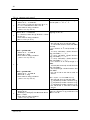
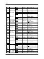
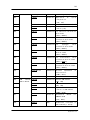
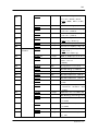
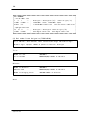
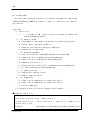
4.2.1.2 EXE> MINimize
group
Items required for energy minimization such as t he method, convergence conditions,
calculation result output, energy terms used in calculation, and boundary/restraint
conditions are specified in this group.
Almost all specifications related to energy calculation are the same as those for
the EXE>MD group.
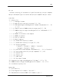
MIN/MD input items
MIN
MD
１
Energy minimization control parameters (same as for STEEP/CONJ)
○
１−１
Control parameters for steepest descent method (STEEP)
○
１−２
Control parameters for conjugate gradient method (CONJ)
○
１−３
Output of calculation results (same as for STEEP/CONJ)
○
１
MD control parameters
○
１−１
Calculation upper limit settings
○
１−２
Time step and number of loop iterations for MD
○
１−３
MD calculation type
○
１−４
Expanded ensemble
○
１−５
Temperature setting
○
１−６
MD calculation conditions
○
１−７
Job restart setting
○
１−８
Calculation result output
○
２
Data output for analysis (energy variation)
２
Data output for analysis (trajectory, parameters)
３
Control parameters related to energy calculation
○
○
３−１
Interaction CUTOFF method
○
○
３−２
Interaction calculation switch
○
○
３−３
Filling Potential method
４
Restraint conditions
○
○
４−１
SHAKE/RATTLE specifications
○
○
４−２
Rigid body model
５
PME, Ewald, FMM specifications
○
○
６
Solvent effect
○
○
７
Boundary conditions
○
○
８
LIST
○
○
９
QUIT
○
○
myPresto 4.2
○
○
○
○
41
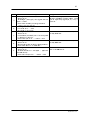
（１）Energy minimization control parameters (same for STEEP/CONJ)
METHODofmini：Energy minimization method（◎）
=STEEpest
；Steepest descent method (Default)
=CONJugate
；Conjugate gradient method
CPUTIMelimit：CPU time upper limit (secs.)（○）
=60.0
；(Default)
LOOPLImit：Number of energy minimization cycles.
If this is 0, the program only calculates energy for initial coordinates.（○）
=0
；(Default)
UPDATEinterval：Update cycle of coordinate information.（△）
If CUTOFF is used for 1 -5 interaction energy, t his designates the update
cycle for the interaction table. In case of periodic boundary conditions,
this designates the update cycle for calculation to correct the
coordinates of an item (which has jumped out of the unit cell) to back
within the cell.
=20
；(Default)
CONVGRadient：Convergence determination condition（△）
If the root mean square summation of force (R.M.S.F.) is less than the
designated value, the calculation is determined to have converged, and
the calculation is terminated. Units (kcal/mol/A)
=0.1
；(Default)
ISTEPLength：Movement distance of atoms in the first step (R.M.S.D.(A) with initial coordinates)
=0.01
；(Default)（△）
（１−１）Control parameters for steepest descent method (STEEP)
This sets step length parameters for the steepest descent method.
UPRATE：If a low energy structure can be obtained in the previous step, this extends
the movement distance by multiplying UPRATE with the step length.
=1.2
；(Default)
DOWNRAte：If energy has increased in the previous step, this reduces the movement
length by multiplying DOWNRATE with the step length.
=0.6：
；(Default)
myPresto 4.2
42
（１−２）Control parameters for conjugate gradient method (CONJ)
This sets search parameters in the conjugate gradient method.
LINESEarchlimit：Number of loop iterations of line search. Do not make this too small.
=10
；(Default)
CONVLInesearch：Threshold value for determining convergence of line search.
Convergence is determined when (DIRGRD/DIRGRS) ≦ CONVL.
DIRGRD : Current Directional Derivative.
DIRGRS : Initial Directional Derivative.
=0.1
；(Default)
（１−３）Calculation result output designation (same for STEEP/CONJ)
MONITOrinterval：Output cycle for standard output
Designates cycle for calculating energy, RMSD etc.（△）
=10
；(Default)
LOGFORmat：Format of standard input（△）
=SHORt
；Simple output within 80 chars. in 1 line (Default)
=DETAil
；Detailed output within 80 chars. in l line. Add each energy.
BESTFItmini：In energy minimization, this provides standard output of RMSD for the
1st chain of the system relative to the reference structure. In the
EXE>INPUT phase, "REFCOORD" or "NAMERE" must be designated as the
reference structure.（△）
=NO
；Do not calculate (Default)
=YES
；Calculate.
（２）Data output for analysis (Energy variation)
MIN energy trajectory
・This outputs energy for each step during energy minimization to a file.
No input designation file.
NAMEAN= (Name of MIN energy trajectory file)
UNITAN：IO Unit of file for MIN energy trajectory
=30
；(Default)
【Note】 the MIN energy trajectory is output for each step.
myPresto 4.2
43
（３）Control parameters relating to energy calculation (same for STEEP/CONJ)
（３−１）Interaction CUTOFF method
CUTMEThod：Interaction CUTOFF method
=RESC ；Residue base cutoff (Default)
Calculates the interactions between all atoms included in residues if the
distance between the residue centers of mass is at or below the CUTOFF distance.
=ATOM ；Atom base cutoff
Calculates the interactions between atoms if the distance between
the atom centers of mass is less than the CUTOFF distance.
=RESA ；Residue base cutoff
Calculates interaction between all atoms included in residues if the minimum
distance between two atoms of a residue is less than the CUTOFF distance.
【Note】 Ordinarily RESA is recommended (if boundary conditions are not periodic).
RESC is recommended for periodic boundary conditions.
CUTLENgth ：Cutoff length（Å）
=8.0
；(Default)
DIEFUNction：Format of relative dielectric function in space
=CONS
；Dielectric function is constant (Default)
=DIST
；Dielectric constant is proportional to the distance.ε=DIEVAL * Distance (Å)
DIEVALue：Dielectric constant of space
=1.0
；(Default)
【Note】 Ordinarily, "DIEVAL=1.0" is used if "DIEFUN=CONS". If "DIEFUN=DIST" is
designated in a vacuum, DIEVAL is set to a value of about 1.0 4.0.
USESPL
；Application of spline interpolation
=NO
；Do not apply（default）
=YES
；Apply
CUT-ON
=6.0
；Spline interpolation start distance
；（default）
【Note】If input topology is CHARM potential, apply spline interpolation by CHARMM.
（３−２）Interaction calculation switch
myPresto 4.2
44
Use the following switch to calculate (or not calculate) a specific interaction.
【Note】 Very Important
・With the 1-5 interaction switch, you must switch energy calculation of van der
Waals/electrostatic interaction/hydrogen bonding between the case when an
interaction table (CUTOFF) is used, and the case when it is not used.
・If you use restraint (CAP, position restraint etc.), you must turn on the switch
for the corresponding energy calculation.
（３−２−１）1-2, 1-3 and 1-4 interaction switches
All default values are used in ordinary MIN/MD calculation. Although it is extremely
rare, this is used only when you do not wish to calculate a certain interaction.
CALBONd：1-2 interaction calculation
=CALC
；Calculate (Default)
=NOCAlc
；Do not calculate
CALANGle：1-3 interaction calculation
=CALC
；Calculate (Default)
=NOCAlc
；Do not calculate
CALTORsion：Torsion interaction calculation
=CALC
；Calculate (Default)
=NOCAlc
；Do not calculate
CALIMProper：Improper torsion calculation
=CALC
；Calculate (Default)
=NOCAlc
；Do not calculate
CALV14：1-4 van der Waals calculation
=CALC
；Calculate (Default)
=NOCAlc
；Do not calculate
CALE14：1-4 electrostatic interaction calculation
=CALC
；Calculate (Default)
=NOCAlc
；Do not calculate
（３−２−２）1-5 interaction switch
This changes the switch designation when calculating using CUTOFF (calculation
using an interaction table), and when calculating all 1 -5 interactions for all atoms
without using CUTOFF (direct calculation). The default setting is to use CUTOFF.
Normally (default), all of the following are calculated: van der Waals, 1-5
electrostatic interaction, and hydrogen bonding. Although it is extremely rare,
please use this only when you do not wish to calculate a certain interaction. If you
use a force field which does not include hydrogen bonds (12-10 Potential), hydrogen
myPresto 4.2
45
bonds are not calculated, regardless of the value of the switch CALHYD. When using
the PME method or Ewald method, please use an interaction table.
When using an interaction table (using CUTOFF)
The following CALV15, CLAE15 and CALHYD are set to =CALC, and CALV5N, CALE5N and
CALH5N are set to =NOCALC. (Default)
CALV15：1-5 van der Waals
=CALC
；Calculate(Default)
=NOCAlc
；Do not calculate
CALE15：1-5 electrostatic interaction calculation
=CALC
；Calculate(Default) ※Mandatory with *PME/FMM
=NOCAlc
；Do not calculate
CALHYD：Hydrogen bonds
=CALC
；Calculate(Default)
=NOCAlc
；Do not calculate
When not using an interaction table
The above CALV15, CLAE15 and CALHYD are set to =NOCALC, and CALV5N, CALE5N and CALH5N
are set to =CALC.
【Note】 With this setting, calculation cannot be done using the PME method, Ewald method
and soft core.
CALV5N：1-5 van der Waals
=NOCAlc
；Do not directly calculate 1-5 van der Waals (Default)
=CALC
；Calculate
CALE5N：1-5 electrostatic interaction
=NOCAlc
；Do not directly calculate 1-5 electrostatic interaction (Default)
=CALC
；Calculate
CALH5N：Hydrogen bonds
=NOCAlc
；Do not directly calculate hydrogen bonds (Default)
=CALC
；Calculate
（３−２−３）Restraint potential
Restraint potential settings are all set to NOCALC (no calculation) by default.
Please set the corresponding energy calculation term when using soft core (soft
repulsion) for CAP restraint, position restraint, distance/angle/torsion restraint
or van der Waals repulsion etc. Also, ordinarily you should designate the applicable
myPresto 4.2
46
atoms for these potentials (see the section on EXE>INPUT), and input parameters where
they are required for force constants etc.
All of these restraint potentials are added to the potential energy term of the
entire system.
CALPSR：Position restraint
=NOCAlc
；Do not calculate(Default)
=CALC
；Calculate
Designate the following in the EXE>INPUT phase.
POSITION=READ
NAMEPO= (Position restraint designation file)
REFCOORD=PDB
NAMERE= (Reference coordinate file)
CALDSR：distance-restraint
=NOCAlc
；Do not calculate(Default)
=CALC
；Calculate
Designate the following in the EXE>INPUT phase.
DISTANcerestrain =READ
NAMEDIstance= (Distance restraint designation file)
CALDHR：dihedral-restraint
=NOCAlc
；Do not calculate(Default)
=CALC
；Calculate
Designate the following in the EXE>INPUT phase.
DIHEDRalrestrain =READ
NAMEDH= (Dihedral restraint designation file)
CALREP：simple repulsion
=NOCAlc
；Do not calculate(Default)
=CALC
；Calculate
CALCAP：CAP restraint
=NOCAlc
；Do not calculate(Default)
=CALC
；Calculate
Designate the following in the EXE>INPUT phase.
SETBOUndary =READ
NAMEBOundary = (CAP boundary designation file)
EXTCAP：ExtendCAP restraint
myPresto 4.2
47
=NOCAlc
；Do not calculate（default）
=CALC
；Calculate
The following is specified in the EXE>INPUT phase:
SETEXC =READ
NAMEEC =（ExtendCAP designated file）
Parameters necessary for restraint potential
Weight factors: With position, distance, repulsion or dihedral restraint, the hardness of the
restraint potential is determined by the temperature and weight etc. If these parameters restrain
the system and the hardness is good and appropriate, then that is generally sufficient. Ordinarily
there is no need to be particularly precise about these values.
TEMPERature: Temperature used for restraint（K）(Position, Distance, Repulsion, Dihedral).
=300.0
；（default）（△）
WETDSR：distance restraint weight
=1.0
；（default）
WETPSR：position restraint weight
=5.0
；（default）
WETDHR：dihedral restraint weight
=10.0
；（default）
Simple repulsion parameters
WETREP：simple repulsion weight
=1.0
；（default）
REPSCAle：van der Waals radius scale factor
=1.0
；（default）
REPDELta：Permissible tolerance
=1.0
；（default）
CAP restraint parameters
To use CAP restraint, a file specifying the atoms subject to CAP restraint (see
the EXE>INPUT section) and "CALCAP=CALC" must be specified, as well as parameters
for the CAP center, CAP radius, and the type and force coefficient of the repulsion
potential which forms the CAP wall. Default values exist, however, the user normally
specifies parameters other than the force constant (FORCAP).
RADCAP： Radius of CAP restraint (A).
myPresto 4.2
48
（The restraint force is 0 inside this radius and is determined by the
potential outside this radius.）
=20.0
：（default）
FORCAP：Force constant of repulsion potential forming the CAP wall
=150.0 ：（default）
FUNCAP：Shape of repulsion potential forming the CAP wall
=HARMonic
： Quadratic parabola potential (default)
=BIQUadratic
F = 0.5 * FORCAP * ( R - RADCAP ) **2
where R = ( center of mass of chain ) - ( CAP center ).
： Biquadratic potential
F = 0.25 * FORCAP * ( R**2 - RADCAP**2 ) **2
where R = ( center of mass of chain ) - ( CAP center ).
SETCEN： Sets center of CAP at center of mass of 1st chain of system.
=NO ： Do not set. Specify the center with CENTRX/CENTRY/CENTRZ (default)
=YES ： Set. Set center of CAP with Cartesian coordinates (A).
CENTRX= 0.0 ：（default）
CENTRY=
CENTRZ=
0.0
0.0
：（default）
：（default）
【Note】If these parameters are specified in both the CAP file and the control file,
the specifications in the control file will take precedence.
【Note】The CAP potential is applied to the center of mass of the molecule or residue.
If the molecule or residue is large, some atoms in the molecule/residue may protrude
outside the CAP radius even if the center of mass is inside the radius.
ExtendCAP restraint parameter
In ExtendCAP restraint, the target atom, target range and force coefficient are
all designated by the ExtendCAP designation file. The control file does not designate
anything other than the Extend designation file （ see the EXE>INPUT chapter ） ,
"EXTCAP=CALC".
（４）Specification of restraint conditions
（４−１）SHAKE/RATTLE
To use SHAKE/RATTLE, a SHAKE file that specifies the atom numbers of the target
atoms and the restraint distance must be specified in the EXE>INPUT group. The
calculation method and convergence conditions are specified in the EXE> MIN group.
SHAKEMethod： Specification of the SHAKE method
=NOSHake ； Do not perform SHAKE（default）
myPresto 4.2
49
=HBON
； Do not perform together with other restraints; calculate as
an independent restraint.
=ALLB
；Calculate all interrelated restraints using the iterative method.
COVSHK：Threshold value for determination of SHAKE convergence.
When ( CBL - IBL ) / IBL is less than this value, SHAKE is determined to
have converged.
CBL: Calculated and corrected bond length, IBL： Input bond length
= 1.0D-6 ；（default）（△）
LIMSHK： Upper limit on number of iterations of SHAKE iterative method
=1000
；（default）（△）
【 Note 】 When restraint conditions that overlap with and interrelate with other
restraints are specified in the SHAKE file, "SHAKEMethod= ALLB" must be used.
【Note】Special restraints in 3 -atom triangle and 4 -atom tetrahedron topologies are
calculated using the iterative method, regardless of the "SHAKEMethod= [HBON ￨
ALLB]" specification.
【Note】 In large systems with extreme deformity, calculation may stop without SHAKE
converging.
【Note】There are restrictions on the range of SHAKE/RATTLE application.
Range of SHAKE/RATTLE application
SHAKE
RATTLE
Energy minimization
Steepest descent method
（METHOD=STEEP）
○
×
（EXE> MIN）
Conjugate gradient method （METHOD=CONJ）
×
×
MD calculation
Leap Frog Verlet（INTEGR=LEAP）
○
×
（EXE> MD）
Velocity-Verlet （INTEGR=VELO）
×
○
Multi Time Step （INTEGR=MTS）
×
×
（５）PME, Ewald, FMM specification
（５−１）Specification of Particle Mesh Ewald method and Ewald method
When a periodic boundary condition is specified, the PME （Particle Mesh Ewald）
method or the Ewald method can be used for the calculation of 1-5 electrostatic
interaction. Only one of the methods can be used.
CALPME： Apply the PME method.
=NOCALC： Do not apply（default）
=CALC ： Apply
PMESPD： Adjust the calculation interval in the PME method.
=NORM ：Calculate every time（default）
myPresto 4.2
50
=HIGH
： Calculate at each "UPDATE" cycle of the coordinate information.
PMEUPD：PMESPD= HIGH calculation method.
=CUT
：Use cut off calculation（default）
Update calculation at each step for short-distance interaction.
Synchronize long-distance interaction calculation with update
cycle “UPDATE” of coordinate information.
=RECI
：Use reversal space term calculation.
Only calculation of interaction for real space is updated at every
step. Calculation of interaction from wavenumber space is
synchronized with update cycle “UPDATE” of coordinate
information.
【 Note 】 The recommended value of PMEUPD option is PMEUPD= CUT. This method is
opportunistic, however, it has better qualities for retaining conserved
quantity.
【Note】Calculation by PMEUPD= RECI has lower qualities for retaining conserved
quantity than PMEUPD= CUT.
CALEWA：Apply the Ewald method.
=NOCALC： Do not apply（default）
=CALC ： Apply
【Note】The PME and Ewald methods require the following specifications:
CALE15= CALC ; For nearby atoms, calculate by the CUTOFF method using the
interaction table.
BOUNDA= PERI ; PME or Ewald can only be used when a periodic boundary condition
is specified.
DIEFUN= CONS ; With PME and Ewald, the spatial dielectric constant of the coulomb
force must be a constant.
PME, Ewald control parameters
EWAPRM：Ewald parameter for the PME, Ewald method
This is a convergence parameter for real space and inverse space. When
increased, real space converges more quickly. When decreased, inverse space
converges more quickly. Specify a value from 0.0 to 1.0.
= 0.35
；（default）
myPresto 4.2
51
REATOL： Permissible tolerance (ε) for cutoff in real space of the Ewald method
（erfc(βＲcut) / Ｒcut ＜ ε）
= 1.0d-19
；（default）
Specification of mesh count in PME
MESHLX= 16
MESHLY= 16
MESHLZ= 16
：X-axis direction (default)
：Y-axis direction (default)
：Z-axis direction (default)
PMEORD： Order of spline function fit when representing charge distribution with mesh points
=5
： Recommended value when EWAPRM = 0.35（default）
【Note】It is best to set the mesh count so that there is a distance of about 1 Å
between mesh points.
（５−２）Specification of Fast Multiple Method
USEFMM：Application of Fast Multipole Method
Specify whether or not the Fast Multipole Method (FMM) is used as a method
for not cutting off the coulomb force. This can be used when there is no periodic
boundary condition.
=NO
；Do not apply FMM（default）
=YES
；Apply FMM.
FMMSPD：Adjustment of calculation interval for 1-5 electrostatic interaction in
the FMM method.
=NORM ：Calculate each time (default)
=HIGH ：Calculate at "UPDATE" cycle of coordinate information.
FMTREE：Tree depth of Fast Multipole Method
Tree depth of the Fast Multipole Method. The number of minimum cells is
8**FMTREE, and the minimum cells are set so that they include several atoms
to several tens of atoms. If stopping due to overflow occurs, increase the
FMTREE value.
= 3
；（default）
FMPOLE： Order of multipoles in Fast Multipole Method
Order of multipoles in the Fast Multipole Method. The larger the FMPOLE value,
the better the accuracy but the slower the speed. However, the effect on speed
is not that great.
myPresto 4.2
52
= 8
；（default）
FMNUMA：Maximum atom number included in minimum cell of Fast Multipole method
= 1000
；（default）
【Note】If the atom number included in the the minimum cell of the Fast Multipole
method exceeds the value specified by the FMNUMA option, an error will occur
And execution of cosgene will stop. In this case, increase the FMTREE option
value or the FMNUMA option value. “DIEFUN=CONS”must be indicated.
（６）Solution effect
（６−１）Specification of Accessible Surface Area method
CALASA：Apply the SA method in the ASA method and the GB/SA method
Apply the accessible surface area method to calculation of the solvation in
the implicit water model.
= NOCALC
；Do not apply（default）
= CALC
；Apply
ASAPRO：Probe radius（Å）
Set the radius for using solvent water for the probe in the ADA method.
Set to approximately 1.4 to 1.6 Å, the radius of a normal water molecule.
= 1.4
；（default）
ASAWEI：ASA weight
Scale factor of contribution to the energy item of the ASA item in the ASA
method.
= 1.0
；（default）
ASACUT：ASA cut-off length (Å)
The distance between atoms used to determine ASA overlapping in the ASA
method.
Specify a length longer than (atom radius ＋ probe radius)×２, however, if the
length is too long, the calculation speed will decrease.
= 4.5
；（default）
【Note】 Do not use solvents such as solvent water or counter ion.
（６−２）Specification of Generalized Born and Surface Area method
The Generalized Born method and the Accessible Surface Area method can be
simultaneously specified (specify both GB calculation "CAL-GB= CALC" and ASA
myPresto 4.2
53
calculation "CALASA= CALC"）to perform calculation by the GB/SA method.
CAL-GB：Use the Generalized Born method
Use the Generalized Born method for calculation of the electrostatic field
in the implicit water model.
= NOCALC
；Do not apply（default）
= CALC
；Apply
CALASA：Use the SA method in the GB/SA method
Use the Surface Area method for calculation of the solvation in the implicit
water model.
= NOCALC
；Do not apply（default）
= CALC
；Apply
GBWELE： Dielectric constant of water
Set the dielectric constant of the solvent water region in the GB method.
This varies depending on the temperature. A dielectric constant near 298 K
is used as the default.
= 78.3
；（default）
GBMELE： Dielectric constant of protein
Set the dielectric constant of the protein region in the GB method.
This varies depending on the temperature and type of protein. Usually a value
from about 1 to 4 is set.
= 1.0
；（default）
GBDELT： Correction value for the Born radius (Å)
Correction value for the Born radius in the GB method (corresponds to "δ"
introduced in Onufriev's work).
Born radius used for calculation = Born radius - GBDELT.
= 0.0
；（default）
GBOFFS：van der Waals radius correction value (Å)
van der Waals radius correction value in the GB method.
van der Waals radius used for calculation = van der Waals radius - GBOFFS.
= 0.09
；（default）
【Note】 The Born radius correction value "GBDELT" corresponds to "δ" introduced
in Onufriev's work. If taken from the work of Still and Hawkins, "GBDELT=0.00".
If taken from the work of Onufriev, "GBDELT=0.15". (For these works, see
"References" at the end of this manual.)
【Note】The default value of the van der Waals radius correction value "GBOFFS"
originates in the work of Still WC (for this work, see "References" at the end
of this manual).
【Note】The Atomic Solvation parameter used in calculation by the ASA method and the
myPresto 4.2
54
GB/SA method changes automatically.
【Note】Do not use solvents such as solvent water or counter ion.
myPresto 4.2
55
（７）Boundary conditions
The boundary conditions which can be used in myPresto are a sphere/ellipsoid, or periodic
boundary conditions (a cell with the 6 faces of a rectangular parallelepiped). A rigid wall which
provides elastic collision is used in a sphere or ellipsoid. Common names are used for some
variables (like designation of the center). When using periodic boundary conditions, be sure
not to forget to designate the cycle (UPDATE) for returning coordinates to the unit cell. In
contrast with CAP restraint, there is no need for a file designating applicable atoms.
BOUNDAry：Boundary condition type
=NO
=PERI
=ELLIPSoid
=SPHERE
；No boundary (Default)
；Periodic boundary conditions
；Ellipsoid boundary
；Sphere boundary
【Note】 Do not designate NO CUTOFF (CAL15N=CALC) for periodic boundary conditions.
Also, RESC is the recommended value. The PME and Ewald methods can be used with
a periodic system, but CUTOFF must be designated.
【Note】 Calculation may stop in the following cases with periodic boundary conditions.
・Switches for the necessary interaction calculation are OFF.
・An unnaturally large force has appeared.
(Potential causes: Strain of initial coordinates, long UPDATE interval, large time step etc.)
・The sum of residue size and CUTOFF distance is larger than half the cell size.
（７−１）Boundary condition center setting
With a periodic system, the boundary condition center is set to the center of mass
of the rectangular unit cell, and with a sphere or ellipsoid, the center is set to
the center of mass of the sphere or ellipsoid.
SETCEN：Sets center of mass of the 1st chain of the system to the center of boundary conditions.
=NO
：Do not apply (Default). Designate with CENTRX/CENTRY/CENTRZ.
=YES ：Apply
If SETCEN=NO, the boundary condition center is designated with Cartesian coordinates
CENTRX=
CENTRY=
CENTRZ=
0.0
0.0
0.0
；(Default)
；(Default)
；(Default)
myPresto 4.2
56
（７−２）Boundary condition size setting
For periodic boundary conditions：
This sets the length along the X, Y and Z axes of the unit cell
LXCELL=
40.0
；(Default)
LYCELL=
40.0
；(Default)
LZCELL=
40.0
；(Default)
For an ellipsoid：
This designates the radius in the X, Y and Z directions, assuming the major and minor
axes of the ellipsoid are aligned with the XYZ coordination directions.
ELLIPA=
30.0
；(Default)
ELLIPB=
30.0
；(Default)
ELLIPC=
30.0
；(Default)
For a sphere：
This designates the radius of the sphere.
RADIUS=
30.0
；(Default)
【Note】 An error will occur if any of the atoms at the initial coordinates are such
that their atomic nucleus is outside the boundary. Be careful because t his is not
the center of mass of the molecule or residue. After starting calculation,
coordinates are corrected and processing is done to return the system inside the
boundary only when the atom goes outside the boundary.
（７−３）Designation of method to pull back coordinates to unit cell
Designate coordinate pull back to a unit cell in a periodical system. Specify atom,
residue, or chain for the unit cell.
REPLAC：coordinate pull back method
=ATOM ：atom unit（default）
=RESI ：residue unit
myPresto 4.2
57
=CHAI ：chain unit
【Note】REPLAC option is enabled only when
BOUNDA= PERI or HEXA.
【Note】If residue base cut off （CUTMET= RESA or RESC）is used with REPLAC= ATOM
specified, coordinates are pulled back by residue unit.
（８）LIST
If you add the command "LIST", current parameter settings will be displayed. No
parameters.
（９）QUIT
This indicates the end of EXE> group input. No parameters.
myPresto 4.2
58
4.2.1.3 EXE> MD group
MIN/MD input items
MIN
MD
１
Energy minimization control parameters ( same for STEEP/CONJ)
○
１−１
Control parameters for steepest descent method (STEEP)
○
１−２
Control parameters for conjugate gradient method (CONJ)
○
１−３
Specification of output of calculation results (same for STEEP/CONJ)
○
１
MD control parameters
○
１−１
Calculation upper limit settings
○
１−２
Designation of time step and number of loop iterations for MD
○
１−３
MD calculation type
○
１−４
Expanded ensemble
○
１−５
Temperature setting
○
１−６
MD calculation conditions
○
１−７
Job restart setting
○
１−８
Specification of output of calculation results
○
２
Analysis data output（energy variation）
２
Analysis data output（trajectory, parameters）
３
Control parameters related to energy calculation
○
○
３−１
Interaction CUTOFF method
○
○
３−２
Interaction calculation switch
○
○
３−３
Filling Potential method
４
Restraint specification
○
○
４−１
Specification of SHAKE/RATTLE
○
○
４−２
Specification of rigid body model
５
Specification of PME, Ewald, FMM
○
○
６
Solvent effect
○
○
７
Boundary conditions
○
○
８
LIST
○
○
９
QUIT
○
○
myPresto 4.2
○
○
○
○
59
（１）MD control parameters
（１−１）Calculation upper limit setting
SETTIMelimit：Simulation time setting (ps).
If the time value (ps) given by "Loop iterations (LOOPLI) x Time
step (TIMEST)" (described below) is large, the calculation is
stopped at the time set here.（◎）
=5.0
；（default）
CPUTIMelimit：Upper limit in CPU time（seconds）（◎）
=60.0
；（default）
（１−２）Specification of MD time step and loop iterations
LOOPLImit：Number of loop iterations for MD simulation（◎）
=0
；（default）
TIMESTep：Time step (fs).
Normally this is 0.5 to 1.0 fs. Set to 1.0 to 2.0 fs when using SHAKE
or rigid model for all H in the system.（◎）
=1.0
；（default）
（１−３）MD calculation type
（１−３−１）Calculation method: Integrator
Method of time integration. When using multi time step（RESPA method), the method of
varying the time step must also be specified.
INTEGR：Method of time integration
=LEAPfrog ；Leap-frog Verlet method（default）
=VELOcity ；Velocity-Verlet method
=MTS
=PRCO
；Multi Time Step (RESPA)
；Predictor-Corrector
=RK4O
；Quartic Runge-Kutta method
=GEAR
；GEAR method
=EXVP
；EXtended phase space Volume Preserving integrator
【Note】In this version, only execution files are provided for Predictor-Corrector,
quartic Runge-Kutta method, GEAR method, and EXtended phase space Volume
Preserving integrator. Source programs are not provided. Therefore, these
functions cannot be used in an execution file obtained by compiling source
myPresto 4.2
60
programs.
When using multi time step, the force f is separated into three types: fa having
a long movement period, fb having an intermediate period, and fc having a short
movement period. The time steps ⊿ta, ⊿tb, and ⊿tc corresponding to each force are
controlled. These time steps are specified by the following relationships using the
calculation frequencies K and L:
⊿tb = K⊿tc,
⊿ta = L⊿tb = LK⊿tc
（K and L are natural numbers）
FREQMEdium: Specify the calculation frequency (interval - medium)
（corresponds
to K in the above equation: ⊿tb = K⊿tc）
；（default）
：Specify the calculation frequency (interval - long)
（corresponds
=1
FREQLOng
=1
to L in the above equation：⊿ta = LK⊿tc）
；（default）
In addition, specify which time step governs each interaction calculation. Specify
in the same way as the next calculation.
CALBON：Calculation of 1-2 interaction
=NOCAlc
=CALC
=MEDIum
；Do not calculate
；Calculate. Governed by time step ⊿tc (default)
；Calculate. Governed by time step ⊿tb
=LONG
；Calculate. Governed by time step ⊿ta
CALANG：Calculation for 1-3 interaction
CALTOR：Calculation for torsion interaction
CALIMP：Improper torsion calculation
CALV14：1-4 van der Waals calculation
CALE14：Calculation for 1-4 electrostatic interaction
CALV15（or CALV5N）：1-5 van der Waals
CALE15（or CALE5N）： for 1-5 electrostatic interaction
CALHYD（or CALH5N）：hydrogen bond
CALPSR：position restraint
CALDSR：distance-restraint
CALDHR：dihedral-restraint
CALREP：simple repulsion
CALCAP：CAP restraint
CALUMB：UMBRELLA potential calculation
myPresto 4.2
61
CALFLW：FLOW potential calculation
CAL-GB：GB calculation
CALASA：ASA calculation
【Note】If "MEDI" or "LONG" is specified for the interaction calculation switch when
other than Multi time step is specified ("INTEGR=MTS"), and error will result and
the program will stop.
【Note】It is best to specify the time step ⊿ta（ "TIMEST"×"FREQME"×"FREQLO" ）
of long-period movement fa so that is does not exceed 4.0 fs.
【Note】When using RATTLE with NVT ensemble, "THERMO= NOSE" must be specified.
【Note】There are limits on the range of application of SHAKE/RATTLE.
Range of application of SHAKE/RATTLE
SHAKE
RATTLE
Energy minimization
Steepest descent method
（METHOD=STEEP） ○
×
（EXE> MIN）
Conjugate gradient method （METHOD=CONJ） ×
×
MD calculation
Leap Frog Verlet（INTEGR=LEAP）
○
×
（EXE> MD）
Velocity-Verlet （INTEGR=VELO）
×
○
Multi Time Step （INTEGR=MTS）
×
×
（１−３−２）Calculation method: Ensemble generation method
METHOD：Specify the ensemble type.
=MICRocanonical ; Micro-canonical(NVE) （default）
=CANOnical
; Canonical(NVT)
=NPT
; NPT
=EXPAnded
=TSAL
; Expanded ensemble
;Tsallis Dynamics
【Note】The NPT ensemble "METHOD=NPT" can only be specified when a periodic boundary
condition is specified.
【Note】Tsalli Dynamics "METHOD=TSAL" is enabled only when the quartic Runge-Kutta
method is used.
（１−３−３）Calculation method: Temperature/Pressure control method
myPresto 4.2
62
THERMOstat：Temperature control method.
This is applied when "METHOD = CANO". Note carefully the range of
application.
=CONStant ; Hoover-Evans Gaussian constraint method （default）
=NOSE
; Nose-Hoover method
COUPLIngtime：Coupling time in the Nose-Hoover method（τ：fs）.
This is applied when "THERMO = NOSE".
=100.0
;（default）
BAROSTat：Pressure control method
This is applied when "METHOD = NPT". Note carefully the range of
application.
=ANDErsen ;Andersen method （default）
=PARA
;Parrinello Rahmann method
SETPRE： Target pressure in NPT（atm）.
= 1.0
；（default）
COUPHB： Coupling time of pressure control in NPT (fs).
= 1000.0
；（default）
COUPPI： Coupling time of pressure control in NPT (fs).
= 1000.0
；（default）
MODIFIcation： Cell shape in NPT. Only effective w hen Parrinello-Rahman method
is specified.
= FLEX
= MONOclinic
= ORTHorhombic
= ISOTropic
；6 degrees of freedom, rhombic cell (default）
； 4 degrees of freedom. Expands and contracts in 3
directions, and the angle of the base cell γ（the angle
formed by the ａ axis and the b axis) changes.
；3 degrees of freedom. Expands and contracts in 3 directions.
；1 degree of freedom. Shape varies isotropically.
= SINGle_direction ；1 degree of freedom. Shape varies only in the z direction.
（１−４）Expanded ensemble method
EXPAND：Specify the expanded ensemble method.
= FORC ： Force-Biased McMD
= SIMU ： Simulated Tempering
= GST ： Generalized Simulated Tempering
= EFFE ： Effective Temperature
（１−４−１）Force-biased Multicanonical MD method
myPresto 4.2
63
RESETC：Step cycle of histogram creation
F.B.McMD is a histogram-based iterative method that recreates the energy
histogram at the step cycle set in "RESETC". If too short, the system does not
search the space sufficiently and the histogram becomes biased. If too long,
a long time is required for calculation. It is best to make "RESETC" longer
for a larger system. For several residue peptides in a vacuum, use a step number
of about 200000 to 400000.
= 300000
；（default）
DUMMYL：Number of dummy loop steps discarded before F.B.McMD is begun.
If starting F.B.McMD from the equilibrium state, set to "１".
= 1
；（default）
TEMMAX：Upper limit (K) of temperature range searched by F.B.McMD.
= 700
；（default）
TEMMIN：Lower limit (K) of temperature range searched by F.B.McMD.
= 250
；（default）
ENEMAX：Upper limit （kcal/mol）of histogram created by F.B.McMD.
The energy distribution at "TEMMAX" must be covered, and thus this should be
set sufficiently higher than the average energy at "TEMMAX". Perform a
canonical calculation using the temperature "TEMMAX" to obtain the average
energy, and set "ENEMAX" to a value higher than this.
= 10000
；（default）
ENEMIN：Lower limit（kcal/mol） of histogram created by F.B.McMD.
The energy distribution at "TEMMIN" must be covered, and thus this should be
set sufficiently lower than the average energy at "TEMMIN". Perform a canonical
calculation using the temperature "TEMMIN" to obtain the average energy, and
set "ENEMIN" to a value lower than this.
= -10000
；（default）
BINSIZ：The bin size (kcal/mol) when a histogram is created with F.B.McMD.
If too fine, the histogram will not be smooth and differentiation will not
be possible. If too rough, it will not be possible to express the shape of the
histogram. It is best to set this to "ENEMAX" - "ENEMIN" divided by about 100
to 200.
= 5.0
；（default）
LIMITS：Threshold determining the range of use of the histogram.
This is the lower limit of the histogram of the energy range sampled by
F.B.McMD. It is best to set LIMITS = LIMITC. Normally a value in the range 0.0005
to 0.001 is set.
= 0.001
；（default）
LIMITC：Threshold for updating the histogram.
myPresto 4.2
64
In the iterative method, the histogram is only updated within the range that
the histogram value is larger than "LIMITC". When the histogram is lower than
"LIMITC", it is considered that there is too much noise and γ cannot be
accurately calculated. "LIMITC" is normally set within the range 0.0005 to
0.001.
= 0.001
；（default）
FBRSTO：Distribution data restart file output format
Specify ASCII or binary format for the output file of distribution d ata (scale
factor, histogram) of F.B.McMD.
=
NOWR
；Do not output （default）
=
ASCI
；ASCII format
=
DOUB
；Double precision binary format
NAMEFO=（Distribution data output file name, 133 characters or less）
FBRSTI：Distribution data restart file input format
Specify ASCII or binary format for the restart-input distribution data (scale
factor, histogram) of F.B.McMD.
NAMEFI= (Distribution data input file name; 133 characters or less）
UNITFR：IO units of distribution data restart file
= 85
myPresto 4.2
；（default）
65
（File example in ASCII format）
# PREVIUS POTENTIAL, LOCAL LOOP, TOTAL LOOP, CURRENT STEP
19.6646786598415
1
# LOCAL HISTGRAM
1
1
351
2.00000000000000
0.000000000000000E+000
：
2.00000000000000
0.000000000000000E+000
# TOTAL HISTGRAM
351
2.00000000000000
1.00000000000000
5.00000000000000
：
4.00000000000000
# PREVIOUS SCALING FACTOR
0.750000000000000
0.750000000000000
1.16322986359255
0.991723974379762
：
0.750000000000000
# BIN-LOWER, BIN-UPPER, PREVIOUS-LOWER, PREVIOUS-UPPER
117
155
112
158
【Note】Set "SETTEM" as the reference temperature for F.B.McMD. The kinetic energy
is fixed at this temperature. Generally this is set higher than "TEMMIN" and lower
than "TEMMAX".
（１−４−２）Simulated Tempering Multicanonical MD method
RESETC：Step cycle for histogram creation
S.T.McMD recreates the coefficient used to determine temperature transition
at the step cycle set in "RESETC". If too short, the system does not search
temperature space sufficiently and the histogram becomes biased. If too long,
a long time is required for calculation. It is best to make "RESETC" longer
myPresto 4.2
66
for a larger system. For several residue peptides in a vacuum, use a step number
of about 200000 to 400000.
= 300000
；（default）
DUMMYL：Number of dummy loop steps discarded before S.T.McMD is begun.
If starting S.T.McMD from the equilibrium state, set to "１".
= 1
；（default）
TEMMAX：Upper limit (K) of temperature range searched by S.T.McMD.
= 700
；（default）
TEMMIN：Lower limit (K) of temperature range searched by S.T.McMD.
= 250
；（default）
ENEMAX：Upper limit of energy histogram created by S.T.McMD（kcal/mol)
The energy distribution at "TEMMAX" must be covered, and thus this should be
set sufficiently higher than the average energy at "TEMMAX". Perform a
canonical calculation using the temperature "TEMMAX" to obtain the average
energy, and set "ENEMAX" to a value higher than this.
= 10000
；（default）
ENEMIN： Lower limit of energy histogram created by S.T.McMD（kcal/mol）
The energy distribution at "TEMMIN" must be covered, and thus this should be
set sufficiently lower than the average energy at "TEMMIN". Perform a canonical
calculation using the temperature "TEMMIN" to obtain the average energy, and
set "ENEMIN" to a value lower than this.
= -10000
；（default）
BINSIZ：The energy bin size (kcal/mol) when an energy histogram is created with S.T.McMD.
= 5.0
；（default）
LIMITS：Threshold determining the range of use of the temperature histogram
This is the lower limit for determination of the temperature range sampled by S.T.McMD.
It is best to set LIMITS = LIMITC. Normally a value in the range 0.0005 to 0.001 is set.
= 0.001
；（default）
LIMITC：Threshold for updating the temperature histogram.
The histogram item γ is used only in the range that the histogram value is
larger than "LIMITC". When the histogram is lower than "LIMITC", it is
considered that there is too much noise and γ cannot be accurately calculated.
"LIMITC" is normally set within the range 0.0005 to 0.001.
= 0.001
；（default）
STTNUM：Temperature division number
The temperature range from TEMMIN to TEMMAX is divided into STTNUM divisions
and S.T.McMD is executed. A more natural temperature transition is expressed
when a higher value is set for STTNUM, however, the sampling time required for
convergence also increases.
= 100
；（default）
STEBAS： Base energy
myPresto 4.2
67
Set the minimum value of the energy that can be taken in by the system. Estimate
this ahead of time by means of a canonical calculation at the temperature
"TEMMIN".
= 0.0
；（default）
【Note】Set "SETTEM" as the reference temperature for S.T.McMD. The kinetic energy
is fixed at this temperature. Generally this is set higher than "TEMMIN" and lower
than "TEMMAX".
（１−４−３）Generalized Simulated Tempering method
Common energy distribution P (E) can be expressed by a Canonical distribution
overlapped at various temperaturesβ i (=1/ｋ B Ｔ i ) by weight Ｆ i . In the Simulated
Tempering method, the ensemble Ξ in which the subensemble Q determined by β is
overlapped by weightＦ(β) has been considered. In Generalized Simulated Tempering,
the parameterλ is introduced and it is expressed by the overlapping of a common
subensemble determined by λ.
GSTMIN：Lower limit of parameter λ
= 0.001d0
；（default）
GSTMAX：Upper limit of parameter λ
= 0.006d0
；（default）
GSTNUM：Number of parameterλ
= 20
；（default）
GSTUPD：Update interval of parameter λ
= 100
；（default）
GSTCON：Parameterλ convergence MD number
= 10000000 ；（default）
GSTSAM：Sampling number before scaling parameterλ
= 50000
；（default）
GSTBAS：Base energy
Set minimum energy value that can be taken by the system.
= 25.5
；（default）
GSTETA：
= 0.5
；（default）
（１−４−４）Effective Temperature method
myPresto 4.2
68
RESETC：Step cycle to preparing histogram
If too short, the histogram deviates because the system temperature space
is not investigated enough. If too long, the histogram takes a long time to
calculate. As the system gets larger, it is desirable to set "RESETC" longer.
In a vacuum, use approximately 200000 to 400000 steps for several peptide
residues.
= 300000
；（default）
ENEMAX：Upper limit of energy histogram prepared by Effective Temperature method
（kcal/mol）.
= 10000
；（default）
ENEMIN: Lower limit of energy histogram prepared by Effective Temperature method
（kcal/mol）.
= -10000
；（default）
BINSIZ：Energy bin size when preparing energy histogram byEffective Temperature method
（kcal/mol）.
= 5.0
；（default）
LIMITS：Threshold to determine the range used by the temperature histogram.
This is the lower limit for determining the temperature range sampled by
the Effective Temperature method. This should be LIMITS= LIMITC. Generally,
the range is 0.0005 to 0.001.
= 0.001
；（default）
LIMITC：Threshold for updating temperature histogram
Termγ of the histogram is used only in the range in which the histogram value
is larger than "LIMITC". If the histogram is lower than "LIMITC", it is
considered that there is too much noise and γ cannot be calculated correctly.
Generally, the range is 0.0005 to 0.001.
= 0.001
；（default）
（１−４−５）Extend ensemble data file output
Designate the file name to which the probability , scale factor, and energy data
is output when Extend ensemble（Effective Temp, Force Bias, Simulated Tempering,
Generalized Simulated Tempering）is used.
NAMEEP：Probability data filename（133 characters or less）
= expand.prob
；（default）
UNITEP：IO units of probability data file
= 78
myPresto 4.2
；（default）
69
NAMEES：Scale factor data file name（133 characters or less）
= expand.scale
；（default）
UNITES：IO units of scale factor data file
= 77
；（default）
NAMEEE：Energy data filename（133 characters or less）
= expand.energy ；（default）
UNITEE：IO units of energy data file
= 79
；（default）
（１−５）Tsallis Dynamics
【Note】In this version, only execution files are provided for Tsallis Dynamics .
Source programs are not provided. Therefore, Tsallis Dynamics cannot be used
in execution files obtained by compiling source programs.
（１−５−１）Setting distribution density function parameters
It is possible to change the distribution density function of Tsallis Dynamics
using the potential energy range.
ELOWER：Low energy side threshold
= 0.0
；（default）
EUPPER：High energy side threshold
= 0.0
；（default）
ROF1DR：Condition of parameter d of ρ１
= 0.5
；（default）
ROF2XI：parameterξ value of ρ２
= 10
；（default）
ROF2VX：Condition of parameterδ ofρ２
= 1000
；（default）
ROF2VY：Condition of parameterγ of row ２
= 0.5
；（default）
（１−５−２）File output option
MNTRZT：Output format of zeta value monitor file
=NO
；Do not output（default）
=ASCI
；ASCII file
myPresto 4.2
70
=SING
；Single precision binary file
=DOUB
；Double precision file
UNITZT：IO units of zeta value monitor file
= 80
；（default）
NAMEZT=（Zeta value monitor file name, 133 characters or less.）
OUTZET：Zeta value monitor file output interval
= 1
；（default）
MNTRCK：Output format of Tsallis integral check value monitor file
=NO
；Do not output（default）
=ASCI
；ASCII file
=SING
；Single precision binary file
=DOUB
；Double precision binary file
UNITCK：IO units of Tsallis integralcheck value monitor file
= 75
；（default）
NAMECK=（Tsallis integral check value monitor filename, 133 characters or less.）
OUTCHK：Tsallis integralcheck value monitor file output interval
= 1
；（default）
MNTRPK：Output format of energy monitor file
=NO
；Do not output（default）
=ASCI
；ASCII file
=SING
；Single precision binary file
=DOUB
；Double precision binary file
UNITPK：IO units of energy monitor file
= 81
；（default）
NAMEPK=（Energy monitor filename, 133 characters or less.）
OUTZPK：Energy monitor file output interval
= 0
；（default）
FLGPKT=（Energy monitor file output item. Potential, kinetic and total energy
are expressed in three characters. "+" is output target, "-" is not
output target.）
MNTRQU：Output format of physical quantity monitor file
=NO
；Do not output（default）
=ASCI
；ASCII file
myPresto 4.2
71
=SING
；Single precision binary file
=DOUB
；Double precision binary file
UNITQU：IO units of physical quantity monitor file
= 82
；（default）
NAMEQU=（Physical quantity monitor filename, 133 characters or less.）
OUTQUA：Physical quantity monitor file output interval
= 1
；（default）
MNTRDO：Output format of Tsallis distribution density function monitor file
=NO
；Do not output（default）
=ASCI
；ASCII file
=SING
；Single precision binary file
=DOUB
；Double precision binary file
UNITDO：IO units of Tsallis distribution density function monitor file
= 82
；（default）
NAMEDO=（Tsallis distribution density function monitor filename, 133 characters
or less.）
OUTDOF：Tsallis distribution density function monitor file output interval
= 1
；（default）
（１−６）Temperature settings
（１−６−１）Target temperature setting
SETTEMperature：Target temperature of system (K).
Target temperature in the fixed temperature ensemble Canonical (NCT) and NPT.
Reference temperature in F.B.McMD. Not used in Micro-canonical(NVE).
=300.0
；（default）
TEMPCOntrol2：Method of system temperature control.
There are two control methods: controlling the temperature (kinetic
energy) of the entire system (TEMPCO=NO), and controlling the temperature
of each molecule (TEMPCO=YES). When TEMPCO=NO, protein and water may have
different temperatures when protein is in water. When TEMCO=YES, it is
easier for different molecules (such as protein and water, and ligand
molecules) to have the same temperature. However, there are cases where
this is unnatural, such as when the temperature of single atom ions is
kept fixed.
myPresto 4.2
72
=NO
；（default）
=YES
（１−６−２）Initial temperature setting
INITIAlvelocity：Method of setting the initial velocity.
=ZERO
=SET
；Initial velocity = 0, Initial temperature = 0 （default）
；Using random numbers defined by RANDOM below, the initial velocity
of each atom is set so that the velocities form a Gaussian
distribution whose mean value is "STARTT".
=RESEt ；Change initial conditions of restart job（refer to （１−７））
STARTTempearture：Mean value of initial temperature (K)
=300.0 ；（default）
RANDOMseed：Random seed number for obtaining velocity distribution
(integer value < 2**31 - 1)
=584287 ；（default）
HEATLOop：Number of iterations of MD loop for raising the temperature using the
Hoover-Evans Gaussian constraint method.
=0
；（default）
（１−７）MD calculation conditions
UPDATEinterval：Update cycle of coordinate information.（△）
When CUTOFF is used for the 1-5 interaction energy, this designates the
update cycle for the interaction table. When a periodic boundary condition
is set, this designates the update cycle for calculation to correct the
coordinates of an atom that has jumped out of a unit cell so that the
coordinates are within the cell.
=20
；（default）
STOPCEnterofmass：Method of fixing center of mass during MD calculation
When applying CAP restraint or a periodic boundary condition, this performs
fixing of the center of mass so that translational or rotational motion
is zero.
=NO
=TRAN
=ROTA
；Do not fix center of mass（default）
；Set translational momentum of 1st chain of system to zero.
；Set rotational momentum of 1st chain of system to zero.
=BOTH ；Set translational and rotational momentum of 1st chain of system to zero.
BESTFIt：Provide standard output of changes in RMSD in the 1st chain of the system
relative to the reference structure in MD. For the reference structure,
"REFCOORD" and "NAMERE" must be specified in the EXE>INPUT phase.（△）
myPresto 4.2
73
=NO
；Do not calculate（default）
=YES
；Calculate
（１−８）Job restart settings
To stop an MD calculation at any step and then restart and continue the calculation,
use the restart file that is output at the end of the job. To restart a job,
specifications for loading the restart file and for resuming calculation are needed.
The initial velocity and initial coordinates of a restart job can be changed.
（１−８−１）Specification of name of restart file: MD calculation before restart
NAMERO：File name of restart file. Binary format.
UNITRO：IO units of restart file
=41
；（default）
【Note】A restart file is always output at the end of MD calculation. If a file name
is not specified, the system default file name will be used.
（１−８−２）Specify loading of restart file: Perform at restart
RESTARt：Restart
=NO ；Do not restart. The initial velocity setting (*see above) is applied（default）
=YES ；Restart.
NAMERI= Name of previously prepared restart file.
UNITRI：IO units of restart file.
=40
；（default）
（１−８−３）Checkpoint setting：Specify the output interval for the automatic
restart file
OUTReSTartfile：CPU time interval for output of automatic restart file.
=0
; Do not output automatic restart file（default）
OUTReStartfileLoop：Loop interval for output of automatic restart file.
=0
; Do not output automatic restart file（default）
【Note】 When OUTRST is specified, output of the automatic restart file takes
place at the CPU time interval for output of automatic restart files.
When OUTRSL is specified, output of the automatic restart file takes
myPresto 4.2
74
place at the loop interval for output of automatic restart files.
【Note】The file name is in the form“name.num”（"name" is the restart file name
specified in the NAMERI option and "num" is a sequence number), and thus
the file is not overwritten.
（１−８−４）Initial condition change： Change the initial velocity and initial
coordinates for restart
Set the initial velocity and initial coordinates for the restart job.
INITIAlvelocity：Method of setting the initial velocity
=ZERO
；Initial velocity = 0, initial temperature = 0（default）
=SET
；Using random numbers defined by RANDOM below, the initial velocity
of each atom is set so that the velocities form a Gaussian
distribution whose mean value is "STARTT"
=RESEt ；Change initial conditions of restart job.
RANDOMseed：Random seed number for obtaining velocity distribution (integer valueRandom seed
number for obtaining velocity distribution (integer value < 2**31 - 1)
=584287 ；（default）
NAMETrajectryIn = Input trajectory file name
NUMberTRJ：Position of coordinate trajectory
=0 ；（default）
（１−９）Specification of result output
Among the intermediate results of MD, this provides standard output of data such
as energy terms, RMSD, temperature, pressure, and CPU time. Monitor output and
trajectories are output to separate files using a different command.
OUTLOG：Number of MD steps for output of intermediate results.
=1
；Output results at each step（default）
LOGFORmat：Output format
=SHORt
；Simple output within 80 characters on 1 line（default）
=DETAil
；Detailed output within 80 characters on 1 line. Each energy is added.
（２）Analysis data input/output (trajectory, parameters)
The following trajectories are all output to files:
myPresto 4.2
75
・MD energy trajectory: Each energy is output to a file at a fixed step cycle of the
MD calculation. There is no input specification file.
・Specified m onitor trajectory: Coordinates of specific atoms, distances between atoms,
angles between atoms, and dihedral angles between atoms are output to a file
at a fixed step cycle of the MD calculation. Perform input specification by
file input and specify "OUTMON" and "NAMEMO" in "EXE>INPUT". Specify atom names
in the control file.
・Coordinate trajectory: The coordinates (only) of all atoms included in the system
(other than fixed atoms) are output to a file at a fixed step cycle of the MD
calculation. There is no input specification file.
・Velocity trajectory: The velocities (only) of all atoms included in the system (other
than fixed atoms) are output to a file at a fixed step cycle of the MD calculation.
There is no input specification file.
・Total energy data: The total potential energy of the system is output to a file
at each step of the MD calculation. There is no input specification file.
MD energy trajectory
MNTRENergy：Format of MD energy trajectory file
=NO
=ASCIi
=SINGle
；Do not output file（default）
；Output in ASCII format
；Output in single-precision binary
=DOUBle ；Output in double-precision binary
OUTENEergy：Output timing
=0
；Every 0 steps (Default)
UNITENergy：IO unit of MD energy trajectory file
=44
；(Default)
NAMEENergy = MD energy trajectory file name
Monitor designation trajectory
MNTRTRajectory：Format of monitor designation trajectory file
=NO
；Do not output file (Default)
=ASCIi
；Output in ASCII format
=SINGle ；Output in single-precision binary
=DOUBle ；Output in double-precision binary
OUTTRJ：Output timing
=0
；Every 0 steps (Default)
myPresto 4.2
76
UNITTR：IO unit of monitor designation trajectory file
=50
；(Default)
NAMETR = Monitor designation trajectory file name
Coordinate trajectory
MNTRCOordinate：Format of coordinate trajectory file
=NO
；Do not output file (Default)
=ASCIi
；Output in ASCII format
=SINGle ；Output in single-precision binary
=DOUBle ；Output in double-precision binary
OUTCOO：Output timing
=0
；Every 0 steps (Default)
UNITCO：IO unit of coordinate trajectory file
=42
；(Default)
NAMECO = Coordinate trajectory file name
Velocity trajectory
MNTRVElocity：Format of velocity trajectory file
=NO：Do not output file (Default)
=ASCIi
；Output in ASCII format
=SINGle ；Output in single-precision binary
=DOUBle ；Output in double-precision binary
OUTVEL：Output timing
=0
；Every 0 steps (Default)
UNITVE：IO unit of velocity trajectory file
=43
；(Default)
NAMEVE = Velocity trajectory file name
Total energy data
MNTRTOtalenergy：Format of total energy data file
=NO
；Do not output file (Default)
=ASCIi
；Output in ASCII format
=SINGle ；Output in single-precision binary
=DOUBle ；Output in double-precision binary
UNITTOtalenergy：IO unit of total energy data file
myPresto 4.2
77
=59
；(Default)
NAMETOtalenergy = Total energy data file name
【Note】 The total energy data file is output for each step of the MD calculation.
（３）Control parameters relating to energy calculation (Same for MIN/MD)
（３−１）Interaction CUTOFF method (Same for MIN/MD)
See the main section on the "EXE>MINimize group".
（３−２）Interaction calculation switch
See the main section on the "EXE>MINimize group".
（３−３）Filling Potential method
CALUMB：Apply or do not apply the Filling Potential method
Specify whether or not the Filling Potential method, a type of umbrella
potential method, is applied. To use the Filling Potential method, a control
file specifying the umbrella potential and the result analysis tool are
necessary.
= NOCALC
；Do not apply（default）
= CALC
；Apply
（４）Specification of restraint conditions
（４−１）Specification of SHAKE/RATTLE
To use SHAKE/RATTLE, a SHAKE file that specifies the atom numbers and restraint
distances of the target atoms must be specified in the EXE>INPUT group. In addition,
the calculation method, convergence conditions, and other information must be
specified in the EXE> MD group.
myPresto 4.2
78
See this item in "EXE> MINimize Group".
（４−２）Specification of rigid body model
The rigid body model allows any atoms of a molecule to be treated as rigid bodies
with internal degrees of freedom fixed. This function is mandatory when using the
TIP4P model. To use the rigid body model, you must specify the molecule and the part
of the molecule to be treated as a rigid body in a rigid-body-model file, or you just
select the automatic mode.
If the automatic mode is selected, the rigid body model is specified as follows.
(a)For a non-water molecule, whose name is not “WAT”.
When a non-hydrogen atom is covalently bound to 1 to 3 hydrogens, they are treated
as a rigid body.
(b)For a water molecule, whose name is “WAT”.
All atoms of the water molecule are treated as a rigid body. The molecule is treated
as TIP3P if the number of atoms is 3 and treated as TIP4P If the number is 4.
RIGIDModel : Specify use of the rigid body model（△）
=NO
；Do not apply rigid body model（default）
=YES
；Apply rigid body model
=AUTO
；Apply automatic rigid body model
UNITRM：IO units of specification file of rigid body model（△）
=58
；（default）
NAMERM =(Rigid body model file name, 80 characters or less.)
If rigid-body is automatically prepared (RIGIDM= AUTO), the prepared information
can be output to a file. The format of the output file is the same as the input file.
DBGRIG：Rigid-body automatic preparation information output designation (△）
=NOWR
；Do not output file（default）
=ASCI
；Output file
UNITDR：IO units of rigid-body automatic preparation information file（△）
=84
：（default）
NAMEDR =(Rigid-body automatic preparation information filename, 133 characters
or less.)
【Note】The rigid body model file can be created using a special tool. The group of
myPresto 4.2
79
atoms to be treated as a rigid body and the 3 -dimensional coordinates to be fixed
are specified in the file. (For the specification procedures, see "A. File Formats"
at the end of this manual.)
（５）Specification of PME, Ewald, FMM
（５−１）Specification of Particle Mesh Ewald method, Ewald method
When a periodic boundary condition is in effect, the PME (Particle Mesh Ewald) method
or the Ewald method can be used to calculate 1 -5 electrostatic interaction. Only one
of the methods can be used.
Refer to this item in "EXE> MINimize Group".
【Note】The following specifications are necessary for the PME method and Ewald method.
CALE15= CALC ; Calculate nearby atoms with the CUTOFF method using an interaction
table.
BOUNDA= PERI ; PME and Ewald cannot be used unless a periodic boundary condition
is in effect.
DIEFUN= CONS ; When using PME or Ewald, the spatial dielectric constant of the
coulomb force must be constant.
（５−２）Specification of Fast Multiple Method
See this item in "EXE> MINimize Group".
（６）Solvent effect（same for MIN and MD）
（６−１）Specification of Accessible Surface Area method（same for MIN/MD）
See this item in "EXE> MINimize Group".
【Note】Solvents such as solvent water molecules and counter ions must not be used.
（６−２）Specification of Generalized Born / Surface Area method（same for MIN/MD）
See this item in "EXE> MINimize Group".
【Note】Solvents such as solvent water molecules and counter ions must not be used.
myPresto 4.2
80
（７）Boundary conditions（same for MIN/MD）
（７−１）Boundary condition center setting（same for MIN/MD）
See this item in "EXE> MINimize Group".
（７−２）Boundary condition size setting（same for MIN/MD）
See this item in "EXE> MINimize Group".
（８）LIST
If list "LIST" is added, the current parameter settings will be displayed. No
arguments.
（９）QUIT
Indicates the end of EXE>Group input.
myPresto 4.2
81
4.2.1.4 EXE> OUTPUT group
The OUTPUT group designates external files for outputting topology files and final
coordinates. Input of these OUTPUT groups is used in common in both "EXE>MIN" and
"EXE>/MD".
【Note】 For the format of each external file, see "A File formats" at the end of
this Manual.
Items designated in the OUTPUT group：
（１）Designation of system topology
（２）Designation of system coordinates
（１）Designation of system topology
TOPOLOgy：Format of topology file（○）
=NOWRite
；No topology file output (Default)
=FORMAtted
；Formatted ASCII file
=BINAry
；Binary file
UNITTOpology：IO unit of topology file（△）
=90
；(Default)
NAMETOpology= (Topology file name. When TOPOLOgy=[FORMIBINA])
（２）Designation of system coordinates
The coordinate file output here outputs coordinates for the N+1st step when the
MD step is N.
COORDInate：Format of 3-dimensional coordinate file in PDB format（○）
=NOWRite
；No coordinate input (Default)
=PDB
；PDB file format
=BINAry
；Binary file
UNITCOordiante：IO unit of coordinate file（△）
=91
；(Default)
NAMECOordinate= (Coordinate file name. When COORD=[PDBIBINA])
（３）QUIT
This indicates the end of EXE> group input.
myPresto 4.2
82
4.2.1.5 EXE> END group
END indicates the end of the cosgene control file.
The only item input is the single line "EXE>END".
myPresto 4.2
83
myPresto 4.2
85
5
Sample calculations
5.1
Sample-1：Peptide in a vacuum
- Calculation of Vassopressin -
（１）Preparing initial coordinate and topology files
Initial coordinates and a topology file in PDB format are required as mandatory
input for MD/energy minimization. These can be prepared using tplgene. Roughly
speaking, there are two ways of preparing these files.
Method 1：Generating the initial coordinates and topology file (in PDB format) by
indicating the amino acid/DNA sequence and its structure to tplgene using
a dihedral angle system
Method 2 ：Generating the initial coordinates and topology file (in PDB format) while
automatically supplementing insufficient atoms with tplgene, using
coordinates in PDB format downloaded from the PDB etc.
Sample-1 provides an explanation of Method 1, and Sample-2 provides an explanation
of Method 2.
（２）Generating initial coordinates and topology file with a dihedral angle system
Create the dihedral angle system input file as "vas.dih".
① Amino acid sequence（PRE>SEQUENCE）
In the lines below "PRE>SEQUENCE", list the amino acid sequence using 3-letter
abbreviations. For N terminal acetylation or C terminal methylation, write ACE/NME,
and if the C terminal is NH2, write "NHE".
② Designation of S-S bonds（PRE>SSBOND）
If the nth residue and the mth residue are bonded with an S -S bond, write the location
of the S -S bond below "PRE>SSBOND" in the form "n m". If there are multiple S -S bonds,
continue to input them on the next line.
③ Designation of dihedral angles（PRE>DIHEDRAL-ANGLES）
Dihedral angles are listed under "PRE>DIHEDRAL-ANGLES". In accordance with the
ECEPP definition, these are listed in the sequenceφ-ψ-ω-χ1-χ2. Please be aware
that in ordinary amino acids, the ω angle is 180°. If you do not understand the
dihedral angles well, in many cases you can obtain a plausible structure via energy
minimization later if you substitute a suitable angle, as indicated in the diagram
below.
myPresto 4.2
86
■Example of input file for dihedral system（vas.dih）
PRE>SEQUENCE
CYS
TYR
PHE
GLN
ASN
CYS
PRO
ARG
GLY
NMECPRE>SSBOND
1
6
PRE>DIHEDRAL-ANGLES
180
180
180
180
180
180
0
0
0
0
0
0
0
0
0
0
0
0
0
0
180
180
180
0
0
0
0
0
0
0
180
180
180
180
180
180
0
0
0
0
0
0
0
0
0
0
0
0
0
0
180
180
180
0
0
0
0
0
0
0
180
180
180
180
180
180
0
0
0
0
0
0
0
0
0
0
0
0
0
0
180
180
180
0
0
0
0
0
0
0
180
180
180
0
0
0
0
0
0
0
In the following example, "vas.dih" generates initial coordinate and topology files
(with the names "vas-dih.pdb" and "vas-dih.tpl") for the molecule "VAS". This section
explains the method of placing the input file and database file in the run-time
directory.
(An example where an arbitrary directory is designated using an environment variable
is given in "5.2 Sample-2".)
■Execution method (Method of placing input file and database file in the run-time directory)
① Copy the input file (assumed here to be "vas.dih"), and the database file to be
used, into the execution directory.
② Execute tplgene in the execution directory. This has no parameters and processing
begins interactively when you type "tplgene".
③ In sequence, input: the title (arbitrary), molecule name (arbitrary), protein or
nucleic acid, input format, database used, input file names, and output file names.
myPresto 4.2
87
■Sample execution
%% Input Title for this molecules %%
If end, type end and (cr).
%% Input Title less than 79 char. %%
Vassopressin test
end
%% Input Molecular Name less than 39 char. %%
If end, type end and (cr).
VAS
end
%% Select Chain Species by the next number. %%
1 : peptide
chain
2 : nucleotide chain
1
%% Select Input File by the next number. %%
1 : pdb
file
2 : dihed file
2
%% Which Force Field Files do you use ? %%
Please choose from the following files .
and write the File Name .
./
C96_aa.tpl
C96_na.tpl
charmm19_aa_all.tpl
charmm22_aa_all.tpl
vas.dih
C96_aa.tpl
%% Input File Name of Atom Coord. or Dihed. %%
./
vas.dih
%% Input File Name of Output Coord. %%
./
vas-dih.pdb
%% Input File Name of Output Topology %%
./
vas-dih.tpl
：
：
%% Program is done. %%
%% This program ended normally. %%
myPresto 4.2
88
5.2
Sample-2: Protein in a vacuum
- Calculation of Lysozyme -
（１）Preparation of initial coordinate and topology files: When using PDB coordinate files
Prepare the initial coordinates of the protein in PDB format. If there is a shortage
of hydrogen (H) it is added automatically. Here it is assumed that "1LZA.pdb" is
downloaded from the PDB. "tplgene" creates the PDB file used in MD, and the topology
file where force field parameters are assigned.
【Note】 Check that molecules are delimited with "TER". If there is no "TER" between
protein chains/molecules, write "TER" into the PDB file yourself.
【Note】 If the molecule is comprised of multiple chains, enter the chain name in
PDB format in front of the residue no. A topology file is created even if there
is no chain name, but multiple molecules with no chemical bonds will be handled
as a single molecule.
【Note】 Only atoms in the ATOM line are subject to processing. The METATM line is
not processed. If a non-standard atom name is designated, the program may stop
processing. In particular, if an irregular name is used for a hydrogen (H) atom,
the system may ignore the given coordinates and recreate a new H at coordinates
built into the program.
【Note】 The types of amino acids which can be processed with tplgene are limited
to those stored in the database. Amino acids other than these are not processed
unless you expand the database yourself.
In the following example, the file in which the HETATM line is removed from
"1LZA.pdb" is treated as "lys_0.pdb". As a result, initial coordinate and topology
files (with the names "lys_1.pdb" and "lys_1.tpl") are created for the molecule called
"LYZ". This section explains the method of handling database files by placing them
in an arbitrary directory.
(An example of the method of placing files in the run-time directory is given in " 5.1
Sample-1".)
■Execution method (Method of placing input file and database file in an arbitrary directory)
① Prepare the input file and database file in an arbitrary directory. Next, set the
path of the directory for the input file, and the directory for the database file,
in environment variables (for the setting method, see "2.2.5 Environment
variables"). If environment variables are not set at the time of tplgene execution,
the directory (input, output or force field DB directory) for the unset variables
will be the current directory.
② Execute tplgene. This has no parameters and processing begins interactively when
you type "tplgene".
③ In sequence, input: the title (arbitrary), molecule name (arbitrary), protein or
nucleic acid, input format, database used, input file names, and output file names.
myPresto 4.2
89
■Sample execution
※In this example, calculation is performed assuming that environmental variables
have been set as follows.
Directory for input file
：/home/user01/myPresto/sample/sample2
Directory for database file
：/home/user01/myPresto/tplgene/DB
%% Input Title for this molecules %%
If end, type end and (cr).
%% Input Title less than 79 char. %%
LYSOZYME test
end
%% Input Molecular Name less than 39 char. %%
If end, type end and (cr).
LYZ
end
%% Select Chain Species by the next number. %%
1 : peptide
chain
2 : nucleotide chain
1
%% Select Input File by the next number. %%
1 : pdb
file
2 : dihed file
1
%% Which Force Field Files do you use ? %%
Please choose from the following files .
and write the File Name .
/home/user01/myPresto/tplgene/DB/
C96_aa.tpl
C96_na.tpl
charmm19_aa_all.tpl
charmm22_aa_all.tpl
C96_aa.tpl
%% Input File Name of Atom Coord. or Dihed. %%
/home/user01/myPresto/sample/sample2/
1LZA.pdb
lys_0.pdb
lys_0.pdb
%% Input File Name of Output Coord. %%
./
lys_1.pdb
%% Input File Name of Output Topology %%
./
lys_1.tpl
(Continued on next page)
myPresto 4.2
90
(Continued from previous page)
INFORMATION> tgReadAminoSequence
Molecule Number
:1
Total number of residues
:129
INFORMATION> tgReadAminoSequence
Amino acid Sequence of the protein
Molecule number :1
LYS+N+ VAL
PHE
GLY
ARG+
CYSS
GLU-
LEU
ALA
ALA
ALA
ARG+
MET
GLY
LYS+
TYR
ARG+
SER
HIS
LEU
GLY
GLY
LEU
ASN
ASPTRP
ASN
VAL
TYR
CYSS
ALA
ALA
LYS+
PHE
GLU-
SER
ASN
PHE
ASN
THR
GLN
THR
ALA
ASP-
THR
TYR
ASN
GLY
ARG+
ILE
ASN
LEU
THR
GLN
ASPILE
GLY
ASN
SER
SER
ARG+
TRP
TRP
CYSS
ASN
ASP-
GLY
ARG+
THR
PRO
GLY
SER
SER
ALA
ARG+
LEU
ASN
LEU
LEU
SER
CYSS
SER
ASN
ASP-
ILE
ILE
PRO
THR
CYSS
ALA
SER
VAL
ASN
CYSS
ALA
LYS+
LYS+
ILE
VAL
SER
ASPTRP
GLY
ARG+
ASN
ASN
GLY
ARG+
MET
CYSS
ASN
LYS+
ALA
GLY
TRP
THR
VAL
ASP-
ALA
VAL
GLN
ALA
TRP
ILE
ARG+
GLY
CYSS
ARG+
LEUC-
INFORMATION> tgReadInputTopology
Amber Type Topology Database File is read
INFORMATION> tgOutputTopology
Write formatted Topology File
INFORMATION> tgSetCoordinate
All the atom positions are now set.
INFORMATION> tgOutputCoordinate
Output pdb-formatted coordinates
CALC. TIME = 0.490000 sec.
%% Program is done. %%
%% This program ended normally. %%
This completes preparation of the protein PDB and topology file.
myPresto 4.2
91
【Note】 For proteins not containing an S-S bond, the PDB ATOM line is sufficient.
However, for molecules containing an S-S bond, tplgene determines the presence
of S-S bonds by reading the line designating S-S bonds in the PDB.
In this example, there is an S-S bond designation line, so "CYS" is replaced with
"CYSS". If the S-S designation line is deleted, "CYS" remains as is, S-S bonds are
not formed, and H is added (as in "S-H"), as indicated in the example below. Please
check whether the conversion has been done correctly.
■Results when S-S bonds have not been designated (Partial)
Molecule number :1
LYS+N+ VAL
ALA
MET
PHE
LYS+
GLY
ARG+
ARG+
HIS
CYS
GLY
GLULEU
LEU
ASP-
ALA
ASN
ALA
TYR
ARG+
GLY
TYR
SER
LEU
GLY
ASN
TRP
VAL
CYS
ALA
GLN
ALA
ALA
LYS+
THR
PHE
ASN
GLUARG+
SER
ASN
ASN
THR
PHE
ASP-
ASN
GLY
THR
SER
THR
ASP-
TYR
GLY
ILE
LEU
GLN
ILE
ASN
SER
ARG+
GLY
TRP
SER
TRP
ARG+
CYS
ASN
ASN
LEU
ASPCYS
GLY
ASN
ARG+
ILE
THR
PRO
PRO
CYS
SER
ALA
LEU
LEU
SER
SER
ASP-
ILE
THR
ALA
SER
ASP-
VAL
GLY
ASN
ASN
CYS
GLY
ALA
MET
LYS+
ASN
LYS+
ALA
ILE
TRP
VAL
VAL
SER
ALA
TRP
ARG+
ASN
ARG+
CYS
LYS+
GLY
THR
ASP-
VAL
GLN
ALA
TRP
ILE
ARG+
GLY
CYS
ARG+
LEUC-
（２）Energy minimization and MD calculation
There are two methods of energy minimization: the steepest descent method and the
conjugate gradient method. However, please be aware that SHAKE cannot be used with the
conjugate gradient method.
Energy minimization is performed in a vacuum using the previous created topology file
and initial coordinates. For interaction, this example uses an 8 Å cutoff and a distance
dependent dielectric function, and updating of the interaction table is done every 20 steps.
In order to observe the displacement of coordinates from initial coordinates as energy
minimization progresses, the following are designated: "REFCOORD=PDB NAMERE=lys_1.pdb"
and "BESTFI=YES". SHAKE cannot be designated with the conjugate gradient method, so a
semi-colon (; ) is used to comment out the "SETSHAKE" line.
If convergence is poor with the conjugate gradient method (i.e. in a large system, or
a system with large strain etc.), it is often better to apply the conjugate gradient method
after first applying the steepest descent method (METHOD=STEEP) for a few tens of steps.
myPresto 4.2
92
■Control file（min_vac.inp）
EXE> INPUT
FORM
PDB
NAMETO=
NAMECO=
lys_1.tpl
lys_1.pdb
REFCOORD=
PDB
NAMERE=
lys_1.pdb
SETSHAKE=
QUIT
READ
NAMESH=
lys.shk
;
TOPOLOGY=
COORDINA=
EXE> MINI
METHOD=
LOOPLI=
CONJ
4000
CPUTIM=
UPDATE=
360000.0
20
MONITO=
5
CONVGR=
0.1D0
CUTMET=
DIEFUN=
RESA
DIST
CUTLEN=
DIEVAL=
8.0D0
2.0D0
BESTFI=
YES
QUIT
EXE> OUTPUT
COORDINATE=
PDB
NAMECO=
lys_1_min.pdb
QUIT
EXE> END
（３）MD calculation
MD is performed, based on the energy minimized coordinates, to achieve the equilibrium
state of the system. The topology file is the same as that used with initial coordinates.
In order to measure the discrepancy from the initial structure, the following are designated
in the control file: "REFCOORD=PDB NAMERE=lys_1.pdb" and "BESTFI=YES".
Now, let's try measuring the distance between amino acid residues in a protein.
Here we create a monitor designation file, and monitor the distance between atom A
and atom B. This is designated as follows.
・Chain no. including A Residue no. in molecule containing A Atom name of A
・Chain no. including B Residue no. in molecule containing B Atom name of B
■Monitor designation file（lys.mntinp）
MONITOR> DISTANCE
1 46 ND2 1 109 CB
1
73
CZ
1 101 CG
END
The above designates the distance between ND2 in the 46th residue and CB in the 109th
residue, and the distance between CZ in the 73rd residue and CG in the 101st residue.
myPresto 4.2
93
To output this to "lys_vac.mnt" in ASCII format every 100 steps, designate
"OUTTRJ=100", "NAMETR=lys_vac.mnt" and "MNTRTR=ASCI".
In addition to the above calculation conditions, the following also indicates input
for NVT calculation at 300K, interaction cutoff at 10Å, fixing translational and
rotational movement of the protein around the center of mass, and random generation
of initial velocities.
The time step setting is normally 0.5fs, and 1.5fs if SHAKE is applied to all hydrogen,
but it is okay to perform NVE calculation beforehand with the same system, and set
to a time step where all energy is saved.
■Control file（md_vac.inp）
EXE> INPUT
TOPOLOGY=
COORDINA=
OUTMONIT=
REFCOORD=
QUIT
EXE> MD
LOOPLI=
SETTIM=
UPDATE=
TIMEST=
OUTTRJ=
OUTLOG=
LOGFOR=
METHOD=
SETTEM=
INITIA=
STARTT=
RANDOM=
FORM
PDB
READ
PDB
2000
500.0D0
20
0.5D0
100
100
DETA
NAMETO=
NAMECO=
NAMEMO=
NAMERE=
lys_1.tpl
lys_1_min.pdb
lys.mntinp
lys_1.pdb
CPUTIM= 3600000.0D0
STOPCE= BOTH
CANONICAL
300.0D0
SET
300.0D0
654321
NAMETR= lys_vac.mnt
BESTFI=
YES
CUTMET=
RESA
DIEFUN=
DIST
CALV15=
CALC
CALE15=
CALC
CALHYD=
NOCALC
CALV5N=
NOCALC
CALE5N=
NOCALC
CALH5N=
NOCALC
QUIT
EXE> OUTPUT
COORDINATE= PDB
QUIT
EXE> END
MNTRTR=
ASCI
CUTLEN=
DIEVAL=
10.0D0
2.0D0
NAMECO=
lys_1_md.pdb
myPresto 4.2
94
5.3
Sample-3: Protein in water
- Calculation of Lysozyme -
（１）Preparation of initial coordinates and topology file
Prepare protein data using the same procedure as for the vacuum case.
In this example, these files are assumed to be "lys_1.pdb" and "lys_1.tpl".
（２）Boundary condition setting
Determine boundary conditions before preparing solvent water. The following 3
boundary conditions can be used.
・Sphere or ellipsoid having a rigid repulsive wall
・CAP water
・Periodic boundary conditions (Cubic cell)
With a sphere or ellipsoid with a rigid repulsive wall, designate the radius (with
the center) for a sphere, or the major/minor axes for an ellipsoid, as indicated below.
Designation is done in the control file. (The following example uses a sphere.) An
ellipsoid is good for calculating the structure in water of a flat, long protein which
deviates from the form of a sphere.
BOUNDARY=
RADIUS=
SPHERE
30.0
CENTRX=
3.500
CENTRY=
CENTRZ=
27.800
34.000
For CAP water, designate the CAP restraint parameters (like CAP center and CAP
restraint radius) in the control file, as indicated below. In the CAP designation file,
designate the protein and water molecules as the object of CAP calculation. In some cases
the CAP center is indicated clearly with coordinates, and in some cases the center of mass
of the molecule is designated. There are two types of repulsion potential , a quadratic
function and a biquadratic function , and the quadratic function is used in this example.
This method is suitable for protein-ligand docking calculation.
CALCAP=
CENTRX=
CALC
3.500
CENTRY=
27.800
CENTRZ=
RADCAP=
34.000
10.0
FORCAP=
20.0
FUNCAP=
SETCEN=
HARMonic
NO
myPresto 4.2
95
■CAP designation file（lys_w.capbc）
BOUND> INCLUDE
LYZ
1
WAT
1
1
YES
4592
YES
Designate periodic boundary conditions in the control file as follows. In addition
to designating the cell center, please designate the length of the cell sides.
BOUNDARY= PERI
CENTRX=
CENTRY=
3.500
27.800
CENTRZ=
34.000
LXCELL=
LYCELL=
20.00
20.00
LZCELL=
20.00
【Note】 For the method of interaction cutoff, please designate "CUTMET=RESC". A
molecule dipole split will occur with ATOM base cut off, so myPresto is designed
so that this feature cannot be used. If the molecule size is close to the cell
size with "CUTMET=RESA", it may be impossible to definitely calculate interactions.
In this case, the program will issue a warning.
myPresto 4.2
96
（３）Generation of water
① Generate water molecules using the program tool "setwater".
(For information on using this tool, see "setwater" in "B Utilities".)
In this example, setwater is used to generate sphericalTIP3P water molecules "wat.pdb" in the region
from the center of mass of the protein "lys_1.pdb" to a radius of 34 Å.
【Note】When adding water, there is a tendency for the density of water molecules to be
somewhat smaller than the actual density due to the form of occupation of the protein
space. If there appear to be gaps in the hydration system after NVT execution, adjust
the number of water molecules. When adding CAP water, arrange molecules (depending on
the system) so that they are somewhat larger than the CAP radius (0.5 to 2 Å). In other
cases, it may be necessary to decrease the damping factor of the vdW radius, or adjust
the density to a slightly higher value.
② Add PDB data for the created water molecules to the protein PDB data, and create
an in-water PDB file. (Add the PDB to the end of the PDB of the target system.)
% cp
lys_1.pdb
lys_w.pdb
% cat wat.pdb >> lys_w.pdb
③ Using the program tool "mergetpl", merge the information in the water molecule
topology file with information in the protein topology file to form a single topology
file. Use the editor to enter the number of water molecules in the merged file.
(For information on using this tool, see "mergetpl" in "B Utilities".)
In this example, a new topology file "lys_w.tpl" is created by merging the protein
"lys_1.tpl" and water " tip3p.tpl" files, and the number of water molecules is entered
in the "MOLECULES" section of "lys_w.tpl".
■Entering the number of water molecules in the topology file "lys_w.tpl"
TPL> TITLE
LYSOZYME test
TPL> MOLECULES
LYZ
WAT
：
（Omitted）
myPresto 4.2
1
4592
；Number of water molecules
97
（４）How to use SHAKE
To execute shake, you must provide myPresto with a SHAKE file describing the SHAKE
conditions. The SHAKE file designates the atoms to be restrained, and the restraint
distance between them. These are designated as follows.
(For details, see the section on SHAKE files in "A Input/Output files".)
・Molecule name
・Number of atoms subject to SHAKE, relative atom no. in molecule of atoms subject
to SHAKE, distance between atoms
■SHAKE file（lys_w.shk）
SHAKE> SHAKE
LYZ
4
1
2
3
1.01000
1.64962
2
5 ->
6
1.01000
8
1.0905
1.01000
1.64962
1.64962
；Distance between atoms
；Number of SHAKE atoms, SHAKE atom number
1.0901
3
；Molecule name
；Number of SHAKE atoms, SHAKE atom number
4 ->
；Distance between atoms
7
9 ->
1.0917
；Number of SHAKE atoms, SHAKE atom number
1.7691
；Distance between atoms
：
：
SHAKE> SHAKE
WAT
3
1
0.95720
；Molecule name
2
3
1.51360
->
0.95720
；Number of SHAKE atoms, SHAKE atom number
；Distance between atoms
The first section above designates SHAKE for 4 atoms. This comprises a tetrahedron, so the
settings designate the distances between 6 atoms. The designation sequence of distances between
atoms is 1-2, 2-3, 3-1 (up to this point, settings are the same as for 3 atoms), 1-4, 2-4 and
3-4. In order to execute SHAKE designated with this SHAKE file, designate "SETSHAKE=READ
NAMESH=lys_w.shk" and "SHAKEM=HBON" in the control file.
【Note】
・Within each line, the part after "; " is a comment. "->" indicates that the line
continues.
・The number of atoms comprising SHAKE is set to 2, 3 or 4.
・SHAKE between multiple molecules cannot be designated.
myPresto 4.2
98
（５）Energy minimization
The following example shows the case where CAP water is used.
■Control file（min_wat.inp）
EXE> INPUT
TOPOLOGY=
FORM
NAMETO=
lys_w.tpl
COORDINA=
PDB
NAMECO=
lys_w.pdb
REFCOORD=
SETBOU=
PDB
READ
NAMERE=
NAMEBO=
lys_w.pdb
lys_w.capbc
SETSHAKE=
READ
NAMESH=
lys_w.shk
QUIT
EXE> MINI
;
;
STEEP
CPUTIM=
360000.0
LOOPLI=
MONITO=
4000
5
UPDATE=
CONVGR=
20
0.2D0
CUTMET=
RESA
CUTLEN=
8.0D0
DIEFUN=
BESTFI=
CONS
YES
DIEVAL=
1.0D0
in case of SPHERE boundary
BOUNDARY=
SPHERE
;
;
;
METHOD=
RADIUS=
35.0
SETCEN=
YES
in case of CAP boundary
CALCAP=
CALC
FUNCAP=
HARMonic
RADCAP=
SETCEN=
34.0
YES
FORCAP=
100.0
SHAKEM=
HBON
QUIT
EXE> OUTPUT
COORDINATE=
PDB
NAMECO=
lys_w_min.pdb
QUIT
EXE> END
【Note】 In boundary conditions for a sphere or ellipsoid, you cannot designate a
sphere region smaller than the atom coordinates included in the input PDB. If there
are atoms outside the boundary conditions, the program will issue a warning and
stop.
myPresto 4.2
99
（６）MD calculation in water
This indicates input for NVT calculation using Gaussian constraint under the restraint given by
the CAP constraint and SHAKE. Equilibrium has not been reached in the first step of MD, so designate
"NAMERO=lys_w_md.res" in the control file, output a restart file and quit.
■Control file（md_wat.inp）
EXE> INPUT
TOPOLOGY=
COORDINA=
OUTMONIT=
REFCOORD=
SETBOU=
SETSHAKE=
QUIT
EXE> MD
LOOPLI=
SETTIM=
UPDATE=
TIMEST=
OUTTRJ=
OUTLOG=
LOGFOR=
;
;
;
;
FORM
PDB
READ
PDB
READ
READ
2000
500.0D0
20
2.0D0
100
10
DETA
NAMETO=
NAMECO=
NAMEMO=
NAMERE=
NAMEBO=
NAMESH=
lys_w.tpl
lys_w_min.pdb
lys.mntinp
lys_w.pdb
lys_w.capbc
lys_w.shk
CPUTIM= 3600000.0D0
STOPCE= BOTH
METHOD=
CANONICAL
THERMO=
SETTEM=
300.0D0
INITIA=
SET
STARTT=
300.0D0
RANDOM=
654321
NAMERO=
lys_w_md.res
in case of SPHERE boundary
BOUNDARY=
SPHERE
RADIUS=
35.0
SETCEN=
in case of CAP boundary
CALCAP=
CALC
FUNCAP=
RADCAP=
34.0
FORCAP=
SETCEN=
YES
NAMETR= lys_wat.mnt
BESTFI=
YES
CUTMET=
RESA
DIEFUN=
CONS
SHAKEM=
HBON
CALV15=
CALC
CALE15=
CALC
CALHYD=
NOCALC
QUIT
EXE> OUTPUT
COORDINATE= PDB
QUIT
EXE> END
CONS
YES
HARMonic
100.0
MNTRTR=
ASCI
CUTLEN=
DIEVAL=
10.0D0
1.0D0
CALV5N=
CALE5N=
CALH5N=
NAMECO=
NOCALC
NOCALC
NOCALC
lys_w_md_1.pdb
myPresto 4.2
100
（７）Restarting
In MD for performing sampling, the usual approach is to restart from the previous MD results.
The coordinates and velocities used for restarting are designated with "RESTARt=YES" and
"NAMERI=lys_w_md.res". Atom names are not written in the restart file, so the coordinates
matching the atom names in the INPUT phase are designated as "COORDINA=PDB NAMECO=lys_w_min.pdb".
■Control file（md_wat2.inp）
EXE> INPUT
TOPOLOGY=
COORDINA=
OUTMONIT=
REFCOORD=
SETBOU=
SETSHAKE=
QUIT
EXE> MD
LOOPLI=
SETTIM=
UPDATE=
TIMEST=
OUTTRJ=
OUTLOG=
LOGFOR=
;
FORM
PDB
READ
PDB
READ
READ
100
500.0D0
20
2.0D0
100
10
DETA
NAMETO=
NAMECO=
NAMEMO=
NAMERE=
NAMEBO=
NAMESH=
lys_w.tpl
lys_w_min.pdb
lys.mntinp
lys_w.pdb
lys_w.capbc
lys_w.shk
CPUTIM= 3600000.0D0
STOPCE= BOTH
RESTARt=
YES
NAMERI=
lys_w_md.res
METHOD=
CANONICAL THERMO=
CONS
SETTEM=
300.0D0
INITIA=
SET
STARTT=
300.0D0
RANDOM=
654321
NAMERO=
lys_w_md_2.res
in case of CAP boundary
CALCAP=
CALC
FUNCAP= HARMonic
RADCAP=
34.0
FORCAP= 100.0
SETCEN=
YES
NAMETR=
lys_wat2.mnt MNTRTR= ASCI
BESTFI=
YES
CUTMET=
RESA
CUTLEN= 10.0D0
DIEFUN=
CONS
DIEVAL= 1.0D0
SHAKEM=
HBON
CALV15=
CALC
CALV5N=
NOCALC
CALE15=
CALC
CALE5N=
NOCALC
CALHYD=
NOCALC
CALH5N=
NOCALC
QUIT
EXE> OUTPUT
COORDINATE= PDB
NAMECO=
lys_w_md_2.pdb
QUIT
EXE> END
myPresto 4.2
101
（８）Log output
Sample output of the calculation log is indicated below.
■Log output
*******************************************************************************
MD LOOP NUMBER
:
LAP CPU TIME
:
(SEC)
TEMPERATURE (K)
TOTAL
KINETIC
20 TIME (PSEC)
:
0.01000
:
0.0000000E+00
(KCAL/MOL) :
-0.4029400E+05
299.9925948 SCALING FACTOR
(KCAL/MOL) :
(KCAL/MOL) :
HAMILTONIAN(NOSE)
:
39.5810551
:
-0.2936448E+05 POTENTIAL
0.1092952E+05
:
:
-0.4029400E+05
0.7281127E+03
ELE14
:
DHR.
:
-0.2936448E+05
TOTAL
TORS.
-(1)
BOND
:
IMPRO. :
0.2342204E+03
0.5763917E+02
ANGLE
VDW14
:
:
0.5456552E+03
0.4271405E+03
0.3779113E+04
VDW15
:
0.3002577E+04
ELE15
:
-0.4906846E+05
0.0000000E+00
REP.
:
0.0000000E+00
CAP.
:
0.0000000E+00
R.M.S.F. (KCAL/MOL*A) :
NAME OF MOLECULE
0.1761278E+02 RMSD (ANGSTROMS)
:
0.2545461E+00
MAX FORCE
TEMPERATURE
CAP ENERGY
LYZ
0.6555757E+02
0.1755462E+03
0.0000000E+00
WAT
0.7155075E+02
0.3165385E+03
0.0000000E+00
INFO>CUTOFF: 1-5 VDW & 1-5 HYD.BOND :
4877928 &
ERROR
-(2)
-(3)
0
*******************************************************************************
（ １ ） Value of the virtual Hamiltonian, which is a conserved quantity in the
Nose-Hoover method.
(However, this is output only when "THERMO=NOSE" is designated.)
（２）RMSD is calculated for atoms in the 1st chain.
In this example, this is RMSD for lysozyme.
（３）The maximum force value, temperature and CAP potential values are displayed
for each molecule.
【Note】 Be careful of the designation of "CALHYD=NOCALC" for different force fields.
With a force field like Amber91 which openly includes the LJ12-10 type potential
of hydrogen bonds, this is set to "CALHYD=CALC". With Amber94/96/99, hydrogen bonds
are included in the Coulomb force, so this is set to "CALHYD=NOCALC".
myPresto 4.2
102
5.4
Sample-4: Expanded ensemble（Force-biased McMD）−Calculation of Alanine peptide−
（１）Force-Biased Multicanonical MD calculation
cosgene can be used to perform Force-Biased Multicanonical MD(F.B.McMD) calculation. Prepare the
protein coordinates and topology file as usual. Using Ace-Ala-Ala-Nme as an example, the dihedral angle
input ala-ala.dih has been prepared as the initial input. First use tplgene to prepare the initial
coordinates ala-ala.pdb and topology file ala-ala.tpl. F.B.McMD is an MD method, and thus cannot be
used for energy minimization. Perform energy minimization in the normal way.
In F.B.McMD, specify expanded ensemble (METHOD= EXPA) and F.B.McMD（EXPAND= FORC). Next, set the
temperature range of the multicanonical distribution that you wish to produce. The range TEMMIN= 250
K to TEMMAX= 700 K is specified in the example. The weight factor for scaling is created from the energy
histogram in F.B.McMD. The range over which the energy histogram is created (ENEMIN to ENEMAX) must
be sufficient to cover the energy distribution of canonical distribution at TEMMIN and the energy range
of canonical distribution at TEMMAX, and thus NVT calculation should be previously performed at TEMMIN
and TEMMAX to obtain approximate values for ENEMIN and ENEMAX.In the example, the energy distribution
at T = 250 K is 20 to 30 kcal/mol, and the energy distribution at T = 700 K is 50 to 70 kcal/mol, and
thus ENEMIN = -100 kcal/mol, ENEMAX = 400 kcal/mol are specified to provide sufficient leeway. Specify
the bin size (BINSIZ) used when the histogram is created. 2 kcal/mol is specified in the example. The
temperature for MD simulation（T0= SETTEM）is the temperature used when the kinetic equation is solved,
and is set such that TEMMIN < SETTEM < TEMMAX. Specify the number of loops (RESETC) per F.B.McMD iteration
and the number of data discard dummy loops (DUMMYL), as well as the overall number of loops (LOOPLI).
LOOPLI should be an integer multiple of RESETC.
■Control file
;fbmcmd_vac.inp
EXE> INPUT
TOPOLOGY=
COORDINA=
OUTMONIT=
REFCOORD=
QUIT
EXE> MD
LOOPLI=
SETTIM=
UPDATE=
TIMEST=
FORM
PDB
READ
PDB
30000000
50000.0D0
20
0.5D0
(Continued on next page)
myPresto 4.2
NAMETO=
NAMECO=
NAMEMO=
NAMERE=
ala_ala.tpl
ala_min.pdb
ala.mntinp
ala_min.pdb
CPUTIM= 3600000.0D0
103
(Continued from previous page)
OUTTRJ=
OUTCOO=
OUTLOG=
LOGFOR=
1000
1000
2000
DETA
METHOD=
RESETC=
TEMMAX=
ENEMIN=
BINSIZ=
SETTEM=
LIMITS=
EXPA
300000
700.0
-100.0
2.0
600.0
0.001
STOPCE= BOTH
EXPAND=
DUMMYL=
TEMMIN=
ENEMAX=
LIMITC=
FORC
1000
250.0
400.0
0.001
INITIA=
STARTT=
RANDOM=
SET
600.0D0
654321
NAMETR=
NAMERO=
NAMECO=
NAMETO=
BESTFI=
ala_vac.mnt
ala_vac.rst
ala_vac.cor
ala_vac.eto
YES
MNTRTR=
ASCI
MNTRCO=
MNTRTO=
SING
ASCI
CUTMET=
DIEFUN=
RESA
DIST
CUTLEN=
DIEVAL=
99.0D0
4.0D0
CALV15=
CALE15=
CALHYD=
CALV5N=
CALE5N=
CALH5N=
QUIT
EXE> OUTPUT
COORDINATE=
QUIT
CALC
CALC
NOCALC
NOCALC
NOCALC
NOCALC
PDB
NAMECO=
ala_md.pdb
EXE> END
When F.B.McMD ends, the expand.energy file, expand.prob file, and expand.scale file
are output along with the coordinate trajectory file. Reweighting analysis for the
purpose of reproducing the canonical distribution is performed using the reweightFB
tool (see "B. Utilities" at the end of this manual) and the expand.scale output file.
myPresto 4.2
104
（２）Reconfiguration of canonical distribution
Prepare the reweightFB analysis tool. Compile as shown below. Analysis is completed
in a short time and thus optimization options are normally not necessary.
% f90 reweightFB.f90
-o reweightFB.x
Prepare the input file inp_MUCA as shown below. Among the files, the ttt3 file is
the most important for reproduction of the canonical distribution.
F.B.scale
ttt1 ttt2 ttt3 ttt4
2.0 251 10 100
600 260 700 20 1.d-05
1st line：Input filename（expand.scale in default）
2nd line：Output file name
1st column：Distribution coefficient
2nd column：Energy, density of state index, entire probability
3rd column：Energy, probability of reweighted canonical distribution
4th column：Temperature, mean energy, square of mean energy, specific heat
3rd line： 1st column：bin size specified in F.B.McMD (=BINSIZ)
2nd column：Data number of histogram (=(ENEMAX-ENEMIN)/BINSIZ + 1)
3rd column：Iteration number at which you wish to begin reweight
4th column：Iteration number at which you wish to end reweight
Normally used until the final iteration (= LOOPLI/RESETC)
4th line： 1st column：T0(SETTEM) used in MD simulation
2nd column：Lower limit of temperature of canonical distribution that you
wish to generate（ > TEMMIN）
rd
3
column：Upper limit of temperature of canonical distribution that you
wish to generate（ > TEMMAM）
th
4
column ： Temperature gradations. "Upper temperature limit - lower
temperature limit" is divided by this number.
th
5
column：Threshold of WHAM analysis. Set to 10-5 or less.
Using the prepared analysis tool and input file, execute with
% reweightFB.x
myPresto 4.2
< inp_MUCA
105
The output file ttt3 is as shown below. The example indicates that a canonical
distribution at 260 K is reproduced by sampling the structure output on the trajectory
at the probability in the second column in the energy range 21 kcal/mol to 61 kcal/mol.
0.260000E+03
0.210000E+02
0.230000E+02
0.250000E+02
0.270000E+02
0.290000E+02
0.310000E+02
0.330000E+02
0.350000E+02
0.370000E+02
0.390000E+02
0.410000E+02
0.430000E+02
0.450000E+02
0.470000E+02
0.490000E+02
0.510000E+02
0.530000E+02
0.550000E+02
0.570000E+02
0.590000E+02
0.610000E+02
0.480194E-04
0.122335E-02
0.917415E-02
0.322814E-01
0.732955E-01
0.126560E+00
0.173496E+00
0.193453E+00
0.173022E+00
0.116629E+00
0.614765E-01
0.263826E-01
0.928163E-02
0.277370E-02
0.708900E-03
0.158080E-03
0.312139E-04
0.549539E-05
0.875144E-06
0.126766E-06
0.167411E-07
Sample 6 explains a method for outputting a representative structure by extracting the structure
from the coordinate trajectory according to this probability distribution.
Cut out only the part for the temperature that you wish to reproduce from the output file ttt3
so as to make a two-column energy and probability distribution file (pdf260_fb) as shown below.
0.210000E+02 0.480194E-04
0.230000E+02 0.122335E-02
0.250000E+02 0.917415E-02
（Middle omitted）
0.510000E+02 0.158080E-03
0.530000E+02 0.312139E-04
0.550000E+02 0.549539E-05
0.570000E+02 0.875144E-06
0.590000E+02 0.126766E-06
0.610000E+02 0.167411E-07
myPresto 4.2
106
5.5
Sample-5：Expanded ensemble (Simulated Tempering McMD) −Alanine peptide calculation−
（１）Simulated Tempering Multicanonical MD calculation
cosgene can be used to perform Simulated Tempering Multicanonical MD (S.T.McMD) calculation. The
following explanation uses the same system as in sample 4. Follow the procedure in sample 4 to perform
the calculations through energy minimization.
To perform S.T.McMD, specify expanded ensemble (METHOD= EXPA) and S.T.McMD （EXPAND= SIMU）. Next,
set the temperature range of the multicanonical distribution that you wish to obtain. The range TEMMIN=
250 K to TEMMAX= 700 K is specified in the example. Perform NVT calculation ahead of time at TEMMIN
and TEMMAX in the same way as for F.B.McMD to determine the ENEMIN, ENEMAX, and BINSIZ parameters for
the energy histogram.
The temperature transition width ΔT will be TEMMAX (maximum temperature) - TEMMIN (minimum
temperature) divided by the temperature division number (STTNUM). The temperature division number
（STTNUM）can be made larger to decrease ΔT and obtain a natural temperature transition, however,
the number of calculations required to sample all temperatures will increase.
The implementation of S.T.McMD in cosgene uses the guide coefficient (E-E0)/kBT2 to calculate the
temperature transition probability. Use the same method as for ENEMIN to obtain an approximate value
for the minimum energy E0 and set the parameter STEBAS to this value. The temperature for performing
MD simulation (T0= SETTEM) is the temperature used when solving the kinetic equation, and is set such
that TEMMIN < SETTEM < TEMMAX. Set the number of loops (RESETC) per S.T.McMD iteration and the number
of data discard dummy loops (DUMMYL), as well as the overall number of loops (LOOPLI). LOOPLI should
be an integer multiple of RESETC.
■Control file
;stmcmd_vac.inp
EXE> INPUT
TOPOLOGY=
COORDINA=
OUTMONIT=
REFCOORD=
QUIT
EXE> MD
LOOPLI=
SETTIM=
UPDATE=
TIMEST=
FORM
PDB
READ
PDB
30000000
50000.0D0
20
0.5D0
(Continued on next page)
myPresto 4.2
NAMETO=
NAMECO=
NAMEMO=
NAMERE=
ala_ala.tpl
ala_min.pdb
ala.mntinp
ala_min.pdb
CPUTIM= 3600000.0D0
107
(Continued from previous page)
OUTTRJ=
OUTCOO=
OUTLOG=
LOGFOR=
1000
1000
2000
DETA
METHOD=
RESETC=
TEMMAX=
ENEMIN=
BINSIZ=
SETTEM=
LIMITS=
STTNUM=
STEBAS=
EXPA
300000
700.0
-100.0
2.0
600.0
0.001
100
-100.0
INITIA=
STARTT=
RANDOM=
NAMETR=
NAMERO=
NAMECO=
NAMETO=
BESTFI=
STOPCE= BOTH
EXPAND=
DUMMYL=
TEMMIN=
ENEMAX=
LIMITC=
SIMU
1000
250.0
400.0
0.001
SET
600.0D0
654321
ala_st.mnt
ala_st.rst
ala_st.cor
ala_st.eto
YES
CUTMET=
DIEFUN=
CALV15=
CALE15=
CALHYD=
CALV5N=
CALE5N=
CALH5N=
QUIT
EXE> OUTPUT
COORDINATE=
QUIT
RESA
DIST
MNTRTR=
ASCI
MNTRCO=
MNTRTO=
SING
ASCI
CUTLEN=
DIEVAL=
99.0D0
4.0D0
CALC
CALC
NOCALC
NOCALC
NOCALC
NOCALC
PDB
NAMECO=
ala_st.pdb
EXE> END
When S.T.McMD ends, the expand.energy file, expand.prob file, and expand.scale file
are output in addition to the coordinate trajectory file. The reference temperature
is output in the log file, and thus the temperature transition state references the
S.T. energy (1st column: energy, 2nd column: temperature). Reweighting analysis for
the purpose of reproducing the canonical distribution is performed by means of the
reweightST tool (see "B. Utilities" at the end of this manual) and the expand.energy
output file.
myPresto 4.2
108
（２）Reconstitution of the canonical distribution
Prepare the reweightST analysis tool. Compile as shown below. Analysis is completed
in a short time and thus optimization options are normally not necessary.
% f90 reweightST.f90
-o reweightST.x
Prepare the input file inp_ST as shown below.
This is the most important canonical file for reproduction of the canonical
distribution.
S.T.energy
average canonical
2.0 250.0 700.0 9.0
1 29999000
600.0
1st column：Input file name（expand.energy in defalt）
2nd column：Output file name
1st column：Mean energy
2nd column：Probability of reweighted canonical distribution
3rd column： 1st column：bin size specified in S.T.McMD (=BINSIZ)
2nd column：Lower limit of distribution output temperature（ > TEMMIN）
3rd column：Upper limit of distribution output temperature（ < TEMMAX）
4th column：Temperature division number. "Upper temperature limit - lower temperature
limit" is divided by this number, calculated, and output.
4th column：1st column：Start of sampling interval（counted from the end of the dummy loop）
2nd column：End of sampling interval（counted from the end of the dummy loop）
5th column：1st column：Reference temperature, SETTEM specified in S.T.McMD
Using the prepared analysis tool and input file, execute with
% reweightST.x
< inp_ST
The output file canonical is as shown below. This was created from the energy
histogram sampled at 362.5K (334.4 K to 390.6K), and indicates that the distribution
is reproduced by sampling the structures output on the trajectory at the probability
in the second column in the energy range 17 kcal/mol to 73 kcal/mol.
myPresto 4.2
109
(Omitted)
362.5000
0.170000E+02
0.190000E+02
0.210000E+02
0.230000E+02
0.250000E+02
0.270000E+02
(Omitted)
0.550000E+02
0.570000E+02
0.590000E+02
0.610000E+02
0.630000E+02
0.650000E+02
0.670000E+02
0.690000E+02
0.710000E+02
0.730000E+02
(Omitted)
0.482616E-06
0.144785E-05
0.231656E-04
0.209455E-03
0.121378E-02
0.491255E-02
0.655827E-02
0.320747E-02
0.141262E-02
0.610027E-03
0.256269E-03
0.112932E-03
0.448833E-04
0.164089E-04
0.337831E-05
0.144785E-05
As with F.B.McMD in Sample 4, cut out only the part for the temperature that you wish
to reproduce from this probability distribution file, and use it in the structure
extraction and clustering of Sample 6（pdf363_st）.
myPresto 4.2
110
5.6
Sample-6：Extend ensemble (Generalized ST McMD)−Calculation of Alanine peptide−
（１）Generalized Simulated Tempering Multicanonical MD calculation
Cosgene
can
calculate
Generalized
Simulated
Tempering
Multicanonical
MD
(G.S.T.McMD). This function can investigate the structure of a wide range of energy
distributions by automatically and optimally shifting between subensembles in
accordance with Tsallis distribution. The system used in sample 4 will be explained.
Calculate until energy is minimized in accordance with the procedure of sample 4.
For G.S.T.McMD, designate Extend ensemble (METHOD= EXPA) and designate G.S.T.McMD
(EXPAND= GST).
The most important parameters for G.S.T.McMD are GSTBAS, GSTETA, GSTMIN, GSTMAX
and GSTNUM. Setting these determines the number of sampled energy ranges and used
subensembles. Determine these numbers taking into consideration the temperature range
to be re-configured later.
At first, determine the safe upper limit temperature
(Tmax) and lower limit temperature (Tmin) so that the temperature range to be
reconfigured is included. Obtain in advance the average potential energy by NVT
calculation in the upper limit and lower limit temperatures.
The multiple subensemble indexλ is the discrete value of GSTMIN∼GSTMAX divided
by the number of GSTNUM. E0 ：GSTBAS is for guaranteeing E-E0 >0 during calculation.
Determine this based on the minimum value of the potential energy in NVT calculation
of Tmin.
If T is effective temperature, T 0 is temperature designated by SETTEMP（reference
temperature）, η is GSTETA, E 0 is GSTBAS, and E is potential energy, the following
relationship holds:
T/T0 =η+λ(E-E0 )
Designate parameters so that the equation provides a value from Tmin/T0 to Tmax/T0.
Set η to
approximately Tmin/T0 . Set GSTMAX so that η+λ(Emax-E0 ) exceeds Tmax/T0
λ and is the upper limit GSTMAX (Emax is determined based on the average potential
energy of NVT calculation in Tmax). Set GSTNUM so that transition between subensembles
becomes smooth for the system.
ENEMIN, ENEMAX and BINSIZ are for preparing a histogram of potential energy.
Determine these so that they do not exceed the range from ENEMIN to ENEMAX during
calculation, as the case of F.B.McMD based on the result of NVT calculation at Tmin
and Tmax.
In order to optimally transfer index λ, the weight ofλ is re-calculated by RESETC.
It is required to set a sufficient size for RESETC depending on the system. GSTUPD
myPresto 4.2
111
becomes the step interval for attempting the transition between subensembles.
myPresto 4.2
112
■Control file
;gstmcmd_vac.inp
EXE> INPUT
TOPOLOGY= FORM NAMETO= ala_ala.tpl
COORDINA= PDB NAMECO= ala_min.pdb
OUTMONIT= READ NAMEMO= ala.mntinp
REFCOORD= PDB NAMERE= ala_min.pdb
QUIT
EXE> MD
LOOPLI= 20000000
SETTIM= 50000.0D0 CPUTIM=3600000.0D0
UPDATE= 20
TIMEST= 0.5D0
OUTTRJ= 1000
OUTCOO= 1000
OUTLOG= 2000
LOGFOR= DETA STOPCE= BOTH
METHOD= EXPA EXPAND= GST
SETTEM= 600.0
RESETC=100000
GSTCON=10000000
GSTBAS=0.0d0
GSTETA=0.3d0
GSTSAM=50000
MNTRXE=ASCI
ENEMIN=0.0
ENEMAX=500.0
BINSIZ=0.5
GSTUPD=100
GSTMIN=0.001d0
GSTMAX=0.015d0
GSTNUM=40
INITIA= SET
STARTT= 600.0D0
RANDOM= 654321
NAMETR=
NAMERO=
NAMECO=
NAMETO=
BESTFI=
ala_gst.mnt MNTRTR= ASCI
ala_gst.rst
ala_gst.cor MNTRCO= SING
ala_gst.eto MNTRTO= ASCI
YES
CUTMET= RESA
DIEFUN= DIST
（Continued）
myPresto 4.2
CUTLEN= 99.0D0
DIEVAL= 4.0D0
113
（Continued）
CALV15= CALC
CALE15= CALC
CALHYD= NOCALC
CALV5N= NOCALC
CALE5N= NOCALC
CALH5N= NOCALC
QUIT
EXE>OUTPUT
COORDINATE=PDB NAMECO=ala_gst.pdb
QUIT
EXE>END
When G.S.T.McMD is completed, the coordinate trajectory file, expand.energy, and
expand.scale file are output. The change in potential energy can be verified in the
first column of expand.energy. The state of transition of λ can be verified in the
third column. Analysis by Reweighting for reproducing the Canonical distribution is
performed by tool reweight GST（refer to the end of the manual ”B utility” for
details） and the output file expand.energy.
myPresto 4.2
114
（２）Reconstruction of canonical distribution
Prepare analysis tool reweight GST. Compile as follows. Analysis is completed in
a short time. Generally, optimization options are not required.
% f90
reweightGST.f90
-o reweightGST.x
Prepare input file inp_GST as shown below.
The ttt3 file is the most important for reproducing canonical distribution.
expand.energy
lambda-pdf lambda-ene-pdf
ttt1 ttt2 ttt3 ttt4
0.5 0.001d0 0.015d0 40 0.0d0 0.3d0
1 18000000
250.0 700.0 50.0 600
1st line: Input filename（default: expand.energy）
2nd line：Output filename
1st column：λ distribution
2nd column ：Energy distribution by λ
3rd line：Output filename
1st column：Partition function
2nd column: Exponent and total probability of energy and density of state,
3rd column: Probability of energy and reweighed canonical distribution
4th column： Square and specific heat of temperature, average energy, square
of average energy, and specific heat
th
4
st
line：1
column：Bin size designated by G.S.T.McMD (=BINSIZ)
2nd column：Lower limit of λ（=GSTMIN）
3rd column：Upper limit of λ（=GSTMAX）
4th column：Number of partitions of λ（=GSTNUM）
5th column：Base energy（=GSTBAS）
6th column：η（=GSTETA）
5th line：1st column：Beginning of sampling interval
2nd column：End of sampling interval (<LOOPLI-GSTNUM*GSTSAM)
For performing preparatory sampling of GSTNUM*GSTSAM step portion.
6th line：1st column：Lower limit of temperature of canonical distribution to be
generated
2nd column ： Upper limit of temperature of canonical distribution to be
generated
myPresto 4.2
115
3rd column：temperature interval
4th column：T0(SETTEM) used for simulation MD
myPresto 4.2
116
Execute using the prepared analysis tool and input file.
% reweightGST.x < inp_GST
The o utput file（ttt3 in this example）is as follows: Sampling the energy structure
shown in the first column from the structure trajectory by the probability in the
second column shows the reproduction of the canonical distribution of 300k.
（Previous lines omitted）
0.300000E+03
0.137500E+02 0.234968E-07
0.142500E+02 0.836684E-07
（Middle lines omitted）
0.577500E+02 0.658355E-07
0.582500E+02 0.430977E-07
0.587500E+02 0.279324E-07
0.592500E+02 0.181532E-07
（Following lines omitted）
As in the case of F.B.McMD of Sample 4, only the temperature l portion to be reproduced
(which is cut out from the probability distribution file) can be used for extracting
the structure and clustering of sample 7.
myPresto 4.2
117
5.7
Sample-7：Expanded sampling−Structure extraction and clustering
（１）Structure extraction using the reconstituted canonical distribution
Energy distributions at any temperature were calculated by reweighting in Sample
4 (F.B.McMD) and Sample 5 (S.T.McMD). In the following, coordinates are extracted
from the trajectory file so as to fill those energy distributions.
The selection analysis tool is used for structure extraction (for detailed information,
see "B. Utilities" at the end of this manual). Prepare the following input file.
pdf363_st
ala_st.cor
S
1000
300000000
0.5
ala_st_363.cor
32
On the 1st line, specify the energy probability distribution file created at the
end of Sample 4 or Sample 5.
On the 2nd line, specify the trajectory file output at the time of MD execution.
The 3rd line is the trajectory file type (Single ￨ Double). This must match the
specification at the time of MD execution.
On the 4th and 5th lines, specify the sampling interval.
On the 6th line, specify the percentage of the structures to be extracted. The
percentage specified here of structures in the sampling interval are output.
On the 7th line, specify the output trajectory file name.
On the 8th line, specify the number of atoms.
Execute with
% selection
< select.inp
myPresto 4.2
118
（２）Structure clustering
Next, the procedure for using cluster analysis to extract representative structures
from the many structures extracted to constitute the canonical distribution in (1)
is explained. Clustering is performed using inter-structure RMSD.
The clustering analysis tool is used for cluster analysis (for detailed information,
see "B. Utilities" at the end of this manual).
First prepare a control file (clustering.inp) similar to the following:
ala_ala.tpl
y
ala_ala.fit
y
ala_ala.rmsd
400
10
1
500
ala_st_363.cor
S
average
ala_st_363.cls
ala_st_363.tree
On the 1st line, specify the topology file.
On the 2nd line, specify whether or not bestfit is applied when RMSD calculation
is performed (y ￨ n).
If bestfit is applied, enter the name of the file that specifies the atoms used
on the next line.
Here a file with the following content is prepared as ala_ala.fit. In this example,
the hydrogen of residue 1-4 of chain 1 is not used for bestfit. This format is the
same as that of the cosgene file that specifies alignment of the system center of
mass. For detailed information, see A.2.11.
SETBST> LIST
FIX 1 1 1 4 H* YES;
myPresto 4.2
119
On the 4th line, indicate (y ￨ n) whether or not there is a specification of atoms used in RMSD
calculation. If there is, on the next line indicate the name of the file that specifies the atoms used
in RMSD calculation. In this example, the file ala_ala.rmsd, which has the same content as ala_ala.fit,
is used. The atoms used in bestfit and RMSD can be checked in the execution log.
On the 6th line, specify the number of structures used for clustering. This will depend on the system,
however, specify a number under 1000. On the 7th line, specify the final number of clusters.
On the 8th and 9th lines, specify the start and end positions of the coordinate trajectory range to
be used.
Specify this trajectory range so that the number of structures specified on the 6th line can be obtained.
In addition, the range should be within the range of the number of structures extracted with the select
tool as described above.
On the 10th line, specify the name of the coordinate trajectory file. In this example, the trajectory
file used to reproduce the canonical distribution with the select tool is used.
On the 11th line, specify the format of the trajectory file（S ￨ D）.
On the 12th line, enter the clustering method（”nearest”￨ “furthest”￨ “median” ￨ “centroid”￨
“average”￨ “flexible”￨ “ward”）.
If "flexible" is specified on this line, set the β value on the next line.
On the 13th line, specify the first name of the output PDB file.
On the 14th line, specify the name of the output dendrogram file.
% clustering < clustering.inp
Execute with the above command. Among the log output items, the number of structures
output per cluster and the mean RMSD express the cluster characteristics well.
（Previous lines omitted）
CLUSTER ID
STRUCTURE COUNT
LOOP NUMBER
RMSD OF AVERAGE
OUTPUT PDB FILE
:
1
:
32
:
16969000
:
1.44551613437161
:ala_st_363.cls.16969000
CLUSTER ID
STRUCTURE COUNT
LOOP NUMBER
RMSD OF AVERAGE
OUTPUT PDB FILE
:
2
:
32
:
8055000
:
1.87505849035797
:ala_st_363.cls.8055000
（Following lines omitted）
myPresto 4.2
120
In addition to the structures of the specified number of clusters (PBX format), a
dendrogram file (PHYLIP format) is output and can be displayed using general tools.
The dendrogram is displayed in three branches: two structures (or clusters) and the
RMSD between them.
23.2573910252864
7.66306178006837
3.26001926531007
79000 44.7507362365723
LOOP 79000, E=44.75
5346000 41.2941055297852
LOOP 5346000, E=41.29
1.88731415528864
RMSD
8076000 47.0816841125488
22555000 49.8077392578125
1.21994863853140
17713000 43.7229232788086
myPresto 4.2
121
5.8
Sample-8：Generation of low molecule topology
−Calculation of Methanol−
（１）Preparation of calculation input file
Topology files of proteins and nucleotides are created with tplgene. By contrast,
tplgeneL is used to create topology files of low-molecule compounds.
There are two general methods for creating topology files of low molecules.
Method 1 ：Create "tplgeneL original format files" based on the charge, bonding order,
and coordinate information obtained by quantum chemistry calculations, and
use those files for calculation.
Method 2 ：Prepare a "Sybyl mol2" file, enter values for the charge information items
in the file, and use the resulting file for calculation.
In the explanation that follows, the environment variables of tplgeneL are set as
shown below (for the setting procedure, see "3.2.6 Environment variables").
TPLL_INPUT_PATH
⇒ ./
Current directory
TPLL_OUTPUT_PATH
⇒ ./
Current directory
TPLL_DB_PATH
⇒ /home/user01/myPresto/tplgeneL/DB
Directory for tplgeneL force field parameter DB
【Note】There are two types of tools for creating tplgeneL original format files:
one for GAMESS output and one for Gaussian output.
（For detailed information, see "B.8 Gamess2tplinp" and "B.9 Gauss2tplinp".）
（２）Generating a topology file from a tplgeneL original format file
The procedure for creating a topology file based on the calculation results of the
quantum chemistry calculation program GAMESS is explained below.
■Execution method
① First perform quantum chemistry calculation of the methanol molecule. Use GAMESS
to perform the calculation, and specify "methnol.log" for the result output file.
② Use the Gamess2tplinp tool to create a tplgeneL original format file from the
"methanol.log" file obtained in ①.
In the execution directory, type in "Gamess2tplinp methanol.log". In this case,
the following three files will be created: "methanol.charge", "methanol.bond", and
myPresto 4.2
122
"methanol.zmat".
%Gamess2tplinp
methanol.log
③ Copy the files obtained in ② to the input file directory.
④ Execute tplgeneL. Type "tplgeneL" without any arguments and start the program
interactively.
%tplgeneL
⑤ Successively specify the file format, input file name, compensation method for
missing parameters, name of the force field parameter DB, and whether or not the
fragment DB will be used.
■Execution example
Please select Input File Format by the next number!
1 : tplgeneL original (*.bond,*.charge,*.zmat)
2 : Sybyl mol2 (*.mol2)
1
Please select Input File Name!
./
ala.bond
ala.zmat
methanol.mol2
phenylalanine.charge
ala.charge methanol.bond
methanol.zmat
phenylalanine.zmat
ala.mol2
methanol.charge phenylalanine.bond xylitol.bond
methanol
What processing do you do if there is a missing parameter?
Please select 1 or 2! (default : 1)
1 : use default parameters.
2 : calculate parameters.
3 : use default parameters when default parameters exist.
use calculated parameters when default parameters don't exist.
1
Please select Input DB Name(prm_gaff.db/prm_amber99.db)!
(default : prm_gaff.db)
/home/user01/myPresto/tplgeneL/DB
angle.prm
bond.prm
nonbond_amber99.db prm_gaff.db
atomtype_amber99.db frg_amber99.db nonbond_gaff.db
atomtype_gaff.db
frg_gaff.db
prm_amber99.db
prm_gaff.db
Do you want to use FragmentDB ? (yes(y)/no(n) default : no)
no
%% Program is done. %%
%% This program ended normally. %%
myPresto 4.2
xylitol.charge
xylitol.zmat
123
（３）Creating a topology file from a Sybyl mol2 file
The procedure for creating a topology file from the Sybyl mol2 file of the desired
low-molecule compound is explained below.
■Execution method
① Prepare a Sybyl mol2 file for the low-molecule compound for which you wish to create
a topology file. Here, this will be the mol2 file ""methanol.mol2" for methanol.
Save "methanol.mol2" in the input file directory specified in the environment
variable.
② Execute tplgeneL. Type "tplgeneL" without any arguments and start the program
interactively.
%tplgeneL
③ Successively specify the file format, input file name, compensation method for
missing parameters, name of the force field parameter DB, and whether or not the
fragment DB will be used.
【Note】tplgeneL does not have a function for adding missing hydrogen atoms. The mol2
file that is prepared must include the hydrogen atom information.
myPresto 4.2
124
■Execution example
Please select Input File Format by the next number!
1 : tplgeneL original (*.bond,*.charge,*.zmat)
2 : Sybyl mol2 (*.mol2)
2
Please select Input File Name!
./
ala.bond
ala.zmat
methanol.mol2
phenylalanine.charge
ala.charge methanol.bond
methanol.zmat
phenylalanine.zmat
ala.mol2
methanol.charge phenylalanine.bond xylitol.bond
methanol
What processing do you do if there is a missing parameter?
Please select 1 or 2! (default : 1)
1 : use default parameters.
2 : calculate parameters.
3 : use default parameters when default parameters exist.
use calculated parameters when default parameters don't exist.
1
Please select Input DB Name(prm_gaff.db/prm_amber99.db)!
(default : prm_gaff.db)
/home/user01/myPresto/tplgeneL/DB
angle.prm
bond.prm
nonbond_amber99.db prm_gaff.db
atomtype_amber99.db frg_amber99.db nonbond_gaff.db
atomtype_gaff.db
frg_gaff.db
prm_amber99.db
prm_gaff.db
Do you want to use FragmentDB ? (yes(y)/no(n) default : no)
no
%% Program is done. %%
%% This program ended normally. %%
myPresto 4.2
xylitol.charge
xylitol.zmat
125
5.9
Sample-9：Free energy calculation（Filling Potential method）−Calculation of methane in water−
（１）Procedure for calculating free energy using the Filling Potential method
In Filling Potential calculation, the stable state where two target molecules are
bound together is taken as the initial structure. An umbrella potential is generated
for one of the molecules in this bound state, causing molecular motion. When this
motion occurs, the locus of the atom designated as the landmark is stored, and at
the next calculation, a repulsive potential is generated around the previous locus.
This allows the establishment of a new locus, not a previous locus, in the next
calculation, enabling calculation that overcomes the potential barrier.
These steps are repeated until the molecules are in a completely dissociated state.
The loci traced up to this point are analyzed by WHAM analysis, allowing the free
energy difference to be obtained.
① MD calculation with an added umbrella potential is performed.
② The umbrella potential of the next MD calculation is generated around the locus.
③ The locus of the landmark atom is extracted and saved.
④ Steps ① to ③ are repeated until a dissociated state is obtained.
⑤ WHAM analysis is performed on the loci obtained to this point.
md_w.inp
Repeat
calculation
until dissociated
MD
Generate_nextFP.inp
Generation of umbrella potential
Extract_atom.inp
Extract locus of landmark atom
ganzine.sh（script）
WHAM_analysis.inp
WHAM Analyis
Figure．Procedure for Free Energy Calculation Using the Filling Potential Method
myPresto 4.2
126
（２）Explanation of sample input file
・Initial coordinate structure
（ch42w.pdb）
・MD calculation input
（md_w.inp）
・Input for umbrella potential update program
（Generate_nextFP.inp）
・Input for landmark atom locus extraction program
（Extract_atom.inp）
・Umbrella potential file
（newopt_fp, newopt_fp_ini）
・Script for execution of entire calculation
（ganzene.sh）
・WHAM analysis program input
（WHAM_analysis.head）
：Prepare the initial structure of the system in
PDB format.
：Input for MD calculation by means of Filling
Potential.
：Input file of program that updates the umbrella
potential.
：Input file of program that extracts the locus of
the landmark atom from the entire locus file.
：Umbrella potential position information file.
Updated as calculation progresses.
： Script that executes the 3 Filling
Potential programs in succession.
：Form of input file for program that analyzes the
locus file calculated by script using the WHAM
method
【Note】The parts that must be changed at the least to calculate another system are
shown in bold in the input file example.
（３）MD calculation with added umbrella potential（cosgene）
To perform MD calculation with an umbrella potential added, specify "CALUMB=CALC"
and "NAMEUM=newopt_fp" in the EXE> MD group of the cosgene control file.
（４）Generate the umbrella potential（Generate_nextFP tool）
Enter the initial center coordinates of the umbrella potential in "newopt_fp_ini".
The umbrella potential coordinates while calculation is in progress and the dimensions
at that time are entered in "newopt_fp". The "newopt_fp" file is also used as input
for the next MD calculations.
■Umbrella potential file
FILL.>GAUS
1 1
6
0.000
0.0300
ATOM 6 CA
potential
myPresto 4.2
；
；
；
；
；
ACE
Specification of unbrella potential shape（ＧＡＵＳ only）
Number of nest and target atom for umbrella potential
Atom number of landmark atom
Height of Gause potential
Width of Gauss potential
2 0.000 0.000 − 2.000
； Coordinates of center of
127
【Note】Do not enter anything after the coordinates of the center of the potential
or a calculation error will result.
The umbrella potential file for the next MD calculation can be generated from the
locus
file
of
the
immediately
previous
MD
calculation
results
using
the
Generate_nextFP tool. This tool generates the next umbrella potential so that the
molecule does not return to the coordinate points of the previous locus. It also sets
the coordinates of the final umbrella potential at the same time.
■Input of Generate_nextFP tool（Generate_nextFP.inp）
newopt_fp
newopt_fp2
initial.pdb
xx_traject.cor
-1000
1000
s
n
HAR1
300.0
0.5
2.5 6.0
3.000
5.0
1.0
ATOM
4131 O
1 50
; Umbrella potential file
; Next umbrella potential file
; Initial coordinates
; Trajectory file name
; Number of trajectory read skips
; Number of trajectory loadings
; Coordinate trajectory file format（ “s”ingle or “d”ouble ）
; Screen display of PDB file
; Shape of centripetal coefficient
; Applicable temperature
; Height of Gauss repulsion factor
; Parameter for adjusting movement distance by RMSD
; Width of Gauss repulsion factor
; Height of centripetal coefficient
; Width of centripetal coefficient
WAT
839
0.000 0.000 -8.000 16.00 -0.83
; Target coordinates for center of umbrella potential（PDB format）
; Number of sweep starts and ends
Target Molecule A
Umbrella Potential 2nd
Potential Target
Umbrella Potential 1st
An umbrella potential is generated
CH4
CH4
CH4
X
so that the molecule does not return
to previous coordinates.
Target Molecule B
dissociation
myPresto 4.2
128
（５）Extraction of locus of landmark atom（Extract_Atom tool）
The Extract_Atom tool is used to extract the locus of the atom that will be the
landmark from the umbrella potential description file and locus file output during
MD calculation.
■Input of Extract_Atom tool（Extract_Atom.inp）
newopt_fp
1033
; Number of all atoms（check initial structure file with "tail" or other
command）
1
; Number of atoms extracted
xx_traject.cor
xx_cont.cor ; Loaded trajectory name＿Output trajectory name
0
; Number of coordinate read skips
2000
; Number of coordinate loadings
s
; Format of coordinate trajectory file（ “s”ingle or “d”ouble ）
【Note】If a large value is used for the number of coordinate loadings, an error will
occur. If an error occurs, try changing this value. The value depends on the entries
in the MD calculation settings file.
（６）Script for executing the entire calculation（ganzene.sh）
This script repeatedly runs the three Filling Potential programs (MD calculation,
umbrella potential generation, and landmark atom extraction). Verify that the file
names are consistent with other input.
■Script（ganzene.sh）
#!/bin/csh
# program directory
set cosgene=/user1/myPresto/cosgene/bin/cosgene
; Change this section as appropriate for your environment.
cp ch42w.pdb initial.pdb
; Initial structure settings
：
rm xx_traject.cor
@ cycle1 = 60
;
Number of calculation cycles
@ counter = 1
;
Initialization of counter
cp newopt_fp_ini newopt_fp
;
Initial umbrella file settings
(Continued on next page)
myPresto 4.2
129
(Continued from previous page)
# program directory
set cosgene=/user1/myPresto/cosgene/bin/cosgene
; Please change this part for your environment
while ($counter < $cycle1)
$cosgene
<
md_w.inp
>
; Loop setting
output
; Execution command for MD calculation
while (! -e final.pdb)
sleep 10
end
sleep 30
; Set to not proceed to the next step
; until the MD calculation loop ends.
;
;
cp final.pdb
mv output
; Copy final structure
; Copy MD calculation output
$GeneFPx
<
w_$counter.pdb
w_$counter.output
$GeneFPinp
>
GeneFP.out
; Update umbrella potential
while (! -e newopt_fp2)
sleep 2
end
mv newopt_fp2 newopt_fp
$Extractx
<
$Extractinp
; Copy output as initial coordinate file
; of umbrella potential.
>
Extract.out
; Extract landmark atom
while (! -e xx_cont.cor)
sleep 3
end
sleep 2
mv xx_cont.cor
w_$counter.cor
mv final.pdb initial.pdb
; Save extracted trajectory
; Copy final structure as initial
; structure of next calculation
myPresto 4.2
130
（７）WHAM Analysis（WHAM_analysis tool）
This tool analyzes the locus files of the extracted landmark atom and calculates
free energy using the WHAM method. Note that if there is insufficient locus file
overlapping, the output values may not be produced. The radius for calculating the
mean energy will also need to be adjusted as appropriate for the size of the system.
■Input of WHAM_analysis tool（WHAM_analysis.inp）
newopt_fp
; Umbrella potential file for the last MD calculation
0
; Number of file read skips
2000
; Number of samplings（depends on MD calculation and number of extracts）
s
; Precision of loaded file（ “s”ingle or “d”ouble ）
1.0
; Radius for calculating mean energy
1000
; Number of WHAM analysis iterations
300.0
; Calculation temperature
m
; Select whether priority is given to memory or speed.
60
; Number of trajectory files
w_1.cor w_1.option ; Trajectory file name and Umbrella potential file name
w_2.cor w_2.option ; Enter all file names one-by-one.
：
w_60.cor w_60.option
The free energy calculation calculates the data point within the radius for
averaging the energy, which is the second value setting from the bottom of the input
file. Adjust the value setting as appropriate for the desired range. The analysis
results are output in the last section of the OUT file.
■Example output file
INFORMATION> WHAM ANALYSIS RESULT
EXP-ID
R.M.S.D(A)
AVERAGE
FREE-ENERGY
1
0.000000
0.000009425
0.712812629E+01
2
0.500101
0.000002134
0.804317891E+01
3
0.410962
0.000006086
0.739754038E+01
4
0.859058
0.000002663
0.790654353E+01
：
：
：
：
：
：
（Structure shear value）（Existence probability distribution（ P(ξ)）（Free
energy value）
The final free energy values that are output are plotted and the PMF is indicated.
The free energy is calculated based on the following equation:
F(ξ) ＝ −ｋTlnP(ξ)
myPresto 4.2
131
k and T are constants that depend on the calculation settings. The P(ξ) value changes
each calculation cycle. If the existence probability is not sufficient, the free
energy
calculation
will
not
be
performed
and
an
error
will
be
displayed: ’-----------------------‘. In this case, it will be necessary to redo
the entire calculation so that sufficient overlapping is obtained, taking such
measures as widening the energy calculation region.
【Note】The WHAM analysis program uses a large amount of memory. Limitations such
as the StackSize may be configured in some calculation environments. Set as large
a StackSize as possible before executing calculation.
【Note】In WHAM analysis of sample 9, please use Wham_AnalysisSample.f90 instead of
Wham_Analysis.f90
to define the distance between the molecules as reaction
coordinates.
myPresto 4.2
132
5.10
Sample-10：RESPA method
MD simulation using multi-time step (RESPA）is explained in the following. First, set the
integration method to multi-time step (INTEGR= MTS). Normally a time-step (= TIMEST) of about 0.5
fsec is used. This will be the short time-step of the most inner side. Multi-time step is a 3-step
operation, integrating over the time step TIMEST in the most inner loop, the time step TIMEST
×FREQME in the second loop, and the time step TIMEST×FREQME×FREQLO in the most outer loop.
The interaction is updated such that the item specified in CALC is updated during the most inner
loop, the item specified in MEDI is updated during the second loop, and the item specified in LONG
is updated during the most outer loop. Normally it is effective to integrate the bonding/angle
parts in the short step （CALBON= CALC, CALANG= CALC）, dihedral angle items in the middle step
(CALTOR= MEDI, CALIMP= MEDI), and electrostatic / van der Waals interaction in the slow step
(CALV14= LONG, CALE14= LONG, CALV15= LONG, CALE15= LONG).
【Note】RESPA is a multistep method of solving the kinetic equation, and thus cannot be used for
energy minimization. In addition, it cannot be used together with SHAKE or the rigid body model.
■Control file
EXE> INPUT
TOPOLOGY=
COORDINA=
OUTMONIT=
REFCOORD=
QUIT
EXE> MD
LOOPLI=
INTEGR=
TIMEST=
FREQME=
FREQLO=
FORM
PDB
READ
PDB
2000
MTS
0.5D0
2
2
NAMETO=
NAMECO=
NAMEMO=
NAMERE=
SETTIM=
UPDATE=
OUTTRJ=
OUTLOG=
LOGFOR=
500.0D0
20
100
200
DETA
METHOD=
SETTEM=
INITIA=
STARTT=
RANDOM=
CANONICAL
300.0D0
SET
300.0D0
654321
(Continued on next page)
myPresto 4.2
;
;
;
;
vas-dih.tpl
vas_min.pdb
vas.mntinp
vas_min.pdb
Specify RESPA method
Time step of most inner side
Most inner side × ２
Most inner side ×２×２
CPUTIM= 3600000.0D0
STOPCE= BOTH
133
(Continued from previous page)
NAMETR= vas_vac.mnt
BESTFI=
YES
CUTMET=
RESA
DIEFUN=
DIST
CALBON=
CALANG=
CALTOR=
CALIMP=
CALV14=
CALE14=
CALV15=
CALE15=
CALC
CALC
MEDI
MEDI
LONG
LONG
LONG
LONG
CALHYD=
CALV5N=
CALE5N=
CALH5N=
QUIT
NOCALC
NOCALC
NOCALC
NOCALC
EXE> OUTPUT
COORDINATE=
QUIT
PDB
MNTRTR=
ASCI
CUTLEN=
DIEVAL=
99.0D0
4.0D0
;
;
;
;
;
;
;
;
Short
Short
Middle
Middle
Long
Long
Long
Long
NAMECO=
vas_md.pdb
EXE> END
myPresto 4.2
134
5.11
Sample-11：RATTLE
−Calculation of indometacin in water−
It is possible to restrain both the position coordinates and velocity in myPresto
by simultaneously specifying the Velocity-Verlet method and the SHAKE method to
execute the RATTLE method.
In this sample, MD calculation of an indometacin-in-water system is performed by
means of the Velocity-Verlet method, which applies the RATTLE method to water
molecules and indometacin.
（１）Preparation of molecules
Use another molecule construction program to create the structure of indometacin.
In the sample, the three-dimensional structure of indometacine has been previously
prepared in PDB format as indo.pdb. In addition, the results of calculation of
indometacin by Gaussian98 have been prepared in indo_g98.out.
First, prepare indo.charge/indo.bond using Gauss2tplinp, and calculate the RESP
charge using the RESP specification file resp.in. The RESP charge calculation tool
can be obtained from the AMBER home page (http://amber.scripps.edu/). Calculate
the RESP charge and then modify the value of the charge of indo.charge or substitute
the RESP charge in the charge item of the mol2 file. When finished, create a topology
file using tplgeneL. Name the indometacin coordinate file, topology file, and mol2
file thus created "indo.pdb", "indo.tpl", and "INDO.mol2".
Next, use the water addition tool setwater to add TIP3P as CAPwater at a radius
of 12 Å centered on the center of mass of indometacin, and name the PDB file
"indo_w.pdb". The topology file of TIP3P is tip3p.tpl, so use the attachment tool
mergetpl to merge the topology file with indo.tpl and thereby create the topology
file "indo_w.tpl" of the indometacin + TIP3P water system.
In addition, for in-water calculation, prepare the file indo_w.capbc which sets
the boundary conditions, and enter the CAP restraint conditions in the control file.
myPresto 4.2
135
（２）Specification of restraint target
As with the SHAKE method, use the SHAKE file to specify the target of restraint
of the RATTLE method. Use the attachment tool SHAKEinp to create the SHAKE restraint
file indo_w.shk from indo_w.pdb and indo_w.tpl.
（For detailed information on SHAKE files, see the SHAKE file section of "A. Input
Files".）
■SHAKE file（indo_w.shk）
SHAKE> SHAKE
indo
4
2
1.1126
1.8434
3
4
5 ->; C
LGD H
LGD
1.1126
1.1135
1.8025
1.8038
2
1.1034
7
8 ->;
C
LGD
H
LGD
2
1.0998
9
10 ->;
C
LGD
H
LGD
2
1.1015
16
17 ->;
C
LGD
H
LGD
2
1.1023
18
19 ->;
C
LGD
H
LGD
2
1.1026
22
23 ->;
C
LGD
H
LGD
2
1.1020
24
25 ->;
C
LGD
H
LGD
4
1.1123
27
28
29
1.7800
1.1127
2
1.0977
33
3
1.1123
35
36
37 ->;
1.7944
1.1137
34 ->;
C
SHAKE> SHAKE
WAT
3
1
2
3
0.95720 1.51360 0.95720
30 ->; C
LGD H
LGD
1.1123
1.8098
1.8049
LGD
H
C
->
H
LGD
H
LGD
H
LGD
H
LGD
LGD
LGD
; O
H
LGD
H1
H
LGD
H2
WAT
myPresto 4.2
136
（３）Control file
To use the RATTLE method, specify the Velocity-Verlet method and SHAKE method
simultaneously. If RATTLE will be applied to all H atoms, set the time step (TIMEST)
to 0.5 to 2.0 fsec.
■Control file（rattle.inp）
EXE> INPUT
TOPOLOGY=
COORDINA=
SETBOU=
SETSHAKE=
NAMESH=
QUIT
EXE> MD
INTEGR=
SHAKEM=
LOOPLI=
SETTIM=
CPUTIM=
UPDATE=
TIMEST=
OUTCOO=
OUTTRJ=
OUTLOG=
LOGFOR=
STOPCE=
METHOD=
THERMO=
SETTEM=
INITIA=
STARTT=
RANDOM=
CALCAP=
RADCAP=
FORCAP=
FUNCAP=
SETCEN=
CUTMET=
DIEFUN=
CALV15=
CALHYD=
CALE5N=
QUIT
EXE> OUTPUT
COORDINATE=
QUIT
EXE> END
myPresto 4.2
FORM
NAMETO=
PDB
NAMECO=
READ
NAMEBO=
READ
; SHAKE
indo_w.shk ; SHAKE
indo_w.tpl
indo_w.pdb
indo_w.capbc
file load command
file name specification
VELO
; Specify Velocity-Verlet method
ALLB
; Specify SHAKE method
10000
5000.0D0
3600000.0D0
20
2.0D0
1000
1000
1000
DETA
TRAN
CANONICAL
NOSE
300.0D0
SET
300.0D0
654321
CALC
10.0
50.0
HARMonic
YES
RESA
CONS
CALC
NOCALC
NOCALC
CUTLEN=
DIEVAL=
CALE15=
CALV5N=
CALH5N=
12.0D0
1.0D0
CALC
NOCALC
NOCALC
PDB
NAMECO=
indo_wmd.pdb
137
5.12
Sample-12：Rigid
−Calculation of indometacin in water−
In this sample, MD calculation of an indometacin-in-water system is performed by
applying the rigid body model to water molecules. Note that the rigid body model can
only be applied to water molecules; currently the TIP3P model and TIP4P model can
be calculated. Other molecules are calculated by calculating all atoms as usual. In
the TIP4P model, the mass of the charge point is zero, and thus cannot be handled
by models other than the rigid body model.
【Note】The rigid body model is only effective when the Velocity-Verlet method is
used for calculation.
（１） File
preparation
Follow the same steps as in Sample 11 to prepare the input file. Generation of TIP4P
water can be performed using the water molecule addition tool setwater. Insert the
water molecule topology file tip4p.tpl into the topology file using mergetpl.
Parameters for the force field in the water molecule are entered in TIP4P, however,
these are not used in the rigid body model.
（２）Specification of rigid body model
The rigid body model file is used to specify the restraint targets of the rigid body
model.（For detailed information on the rigid body model file, see the rigid body
model file section of "A. Input Files".）
■Rigid body model file（indo_w4.rig）
myPresto 4.2
138
RIGID>
indo
4
2
2
2
2
2
2
4
2
3
NUMBER
2
7
9
16
18
22
24
27
33
35
3
8
10
17
19
23
25
28
34
36
RIGID> COOR
WAT
4 ->
1
0.000
2
0.757
3
-0.757
4
0.000
4
5
29
30
37
0.000
0.586
0.586
0.150
0.000 ->
0.000 ->
0.000 ->
0.000
（３）Control file
To use the rigid body model, use of the rigid body model and the rigid body model
file name must be specified in the MD phase of the control file. If H atoms that have
not been made rigid remain in the system, set the time step (TIMEST) to about 0.5
fsec.
myPresto 4.2
139
■Control file（rigid.inp）
EXE> INPUT
TOPOLOGY=
COORDINA=
SETBOU=
QUIT
EXE> MD
RIGIDM=
NAMERM=
INTEGR=
LOOPLI=
SETTIM=
CPUTIM=
UPDATE=
TIMEST=
OUTCOO=
OUTTRJ=
OUTLOG=
LOGFOR=
METHOD=
SETTEM=
INITIA=
STARTT=
RANDOM=
CALCAP=
RADCAP=
FORCAP=
FUNCAP=
SETCEN=
CUTMET=
DIEFUN=
CALV15=
CALHYD=
CALE5N=
QUIT
EXE> OUTPUT
COORDINATE=
QUIT
EXE> END
FORM
PDB
READ
NAMETO=
NAMECO=
NAMEBO=
YES
indo_w4.rig
VELO
10000
5000.0D0
3600000.0D0
20
2.0D0
1000
1000
1000
DETA
CANONICAL
300.0D0
SET
300.0D0
654321
indo_w4.tpl
indo_w4.pdb
indo_w4.capbc
; Specify use of rigid body model
; Specify rigid body model file name
; Specify Velocity-Verlet method
CALC
10.0
50.0
HARMonic
YES
RESA
CONS
CALC
NOCALC
NOCALC
CUTLEN=
DIEVAL=
CALE15=
CALV5N=
CALH5N=
12.0D0
1.0D0
CALC
NOCALC
NOCALC
PDB
NAMECO=
indo_w4md.pdb
myPresto 4.2
140
5.13
Sample-13：Calculation of periodic systems using NPT and PME −Calculation of methane in water−
【Andersen method】
In this sample the NPT ensemble and Andersen methods are used to calculate a periodic boundary
system consisting of two methane molecules in a unit cell filled with water.
The system is created by generating water molecules around the two methane molecules using
the set_water tool. Each side of the three-dimensional unit cell is 18.64775 Å.
As a basic principle, SHAKE cannot be used for NPT calculation. Here calculation is performed
with All Atom. Specify "METHOD=NPT", and specify the Velocity-Verlet method ("INTEGR=VELO") for
the integrator. The Andersen method is used, and thus "BAROST=ANDE" is specified. In the Andersen
method, only isotropic cells are transformed. Specify "MODIFI=ISOT" so that the option for
specifying the cell shape is always isotropic cell transformation with one degree of freedom.
As calculation will be performed using the boundary condition of a periodic system, specify
"BOUNDA=PERI" for the boundary condition setting.
The target pressure "SETPRE" is 1 atmosphere in this sample.
The relaxation time setting depends on the system, however, it is generally best to set the
relaxation time of temperature control "COUPHB" to about 100 to 500 fsec, and the relaxation
time of pressure control "COUPPI" to several times the relaxation time of temperature control,
or about 1000 to 5000 fsec.
1-5 electrostatic interaction is calculated using the Particle-Mesh-Ewald (PME) method. For
the PME settings, "CALPME=CALC" is specified, and "CUTLEN" is set so as to openly calculate the
electric field, requiring a value of about 6 to 8 Å, or less than half the length of a side
of the unit cell. The number of mesh nodes are set in "MESHLX", "MESHLY","MESHLZ" for the X,
Y, and Z axes. A value of 1 to 3 Å is reasonable for the mesh width, as a short width increases
precision but also lengthens the calculation time. In the sample, "MESHLX=18" is specified
（same for "MESHLY" and "MESHLZ） so as to partition the side length of 18.64775 Å into mesh
nodes of about 1 Å. The Ewald parameter "EWAPRM" may affect precision depending on the system,
and a value of 0.35 is generally set. Specifying a low value for the order "PMEORD" of the
polynomial for interpolation from the grid potential will make calculation quicker but decrease
precision, while specifying a high value will increase precision but decrease speed. This value
is set to about 3 to 6. PME is a no-cutoff method, however, this does not mean that calculation
is performed without creating an atom interaction table; an atom interaction table is created
to calculate nearby electrostatic interaction and thus "CALE15=CALC", "CALE5N=NOCALC",
myPresto 4.2
141
"CALV15=CALC", "CALV5N=NOCALC", and "CALH5N=NOCALC" are specified.
■Control file
EXE> INPUT
TOPOLOGY=
COORDINA=
REFCOORD=
QUIT
EXE> MD
LOOPLI=
SETTIM=
UPDATE=
TIMEST=
OUTLOG=
STOPCE=
FORM
PDB
PDB
2000000
5000.0D0
10
0.5D0
1000
NO
METHOD=
INTEGR=
BAROST=
MODIFI=
SETPRE=
COUPHB=
COUPPI=
NPT
VELO
ANDErsen
ISOT
1.0
100.0
2000.0
SETTEM=
INITIA=
STARTT=
CUTMET=
DIEFUN=
300.0D0
SET
300.0D0
RESC
CONS
BOUNDA=
LXCELL=
SETCEN=
CENTRX=
PERI
18.64775
NO
0.0
NAMETO=
NAMECO=
NAMERE=
initial.tpl
initial.pdb
initial.pdb
;1000 psec
CPUTIM=
LOGFOR=
3600000.0D0
DETA
; NPT
; Velocity-Verlet
; Andersen
RANDOM=
654321
CUTLEN=
DIEVAL=
8.0D0
1.0D0
LYCELL=
18.64775
LZCELL=
18.64775
CENTRY=
0.0
CENTRZ=
0.0
MESHLZ=
18
; for PME
CALPME=
EWAPRM=
MESHLX=
PMEORD=
CALC
0.35
18
6
PMESPD=
HIGH
MESHLY=
18
CALV15=
CALE15=
CALHYD=
QUIT
CALC
CALC
NOCALC
CALV5N=
CALE5N=
CALH5N=
NOCALC
NOCALC
NOCALC
EXE> OUTPUT
COORDINATE=
QUIT
EXE> END
PDB
NAMECO= final.pdb
myPresto 4.2
142
【Parrinello-Rahmann method】
In this sample the NPT ensemble and Parrinello-Rahmann methods are used to calculate a periodic
boundary system consisting of two methane molecules in a unit cell filled with water.
The system is created by generating water molecules around the two methane molecules using
the set_water tool. Each side of the three-dimensional unit cell is 18.64775 Å.
As a basic principle, SHAKE cannot be used for NPT calculation. Here calculation is performed
with All Atom. Specify "METHOD=NPT", and specify the Velocity-Verlet method ("INTEGR=VELO") for
the integrator. The Parrinello-Rahmann method is used, and thus "BAROST=PARA" is specified. In
the Parrinello-Rahmann method, transformation of anisotropic cells is allowed. The five
selections below are available for the option "MODIFI", which specifies the cell shape.
MODIFI = FLEX
；6 degrees of freedom, rhombic cell（default）
= MONOckinic
；4 degrees of freedom, extension/contraction in 3 directions,
angle γ of base cell (angle between a and b axes) changes
= ORTHorhombic
；3 degrees of freedom, extension/contraction in 3 directions
= ISOTropic
；1 degree of freedom, isotropic change. Resembles Andersen method.
= SINGle_direction ；1 degree of freedom, change only in direction of z axis
In the Parrinello-Rahmann method, the boundary condition setting "BOUNDA" is always set to
"BOUNDA=HEXA", regardless of the "MODIFI" specification.
【Note】Set the periodic boundary condition to "BOUNDA=HEXA", not "BOUNDA=PERI".
The target pressure "SETPRE" is 1 atmosphere in this sample.
The relaxation time setting depends on the system, however like the Andersen method, it is
generally best to set the relaxation time of temperature control "COUPHB" to about 100 to 500
fsec, and the relaxation time of pressure control "COUPPI" to several times the relaxation time
of temperature control, or about 1000 to 5000 fsec.
PME is specified in the same way as for the Andersen method in the previous section. The cell
shape changes during NPT, and thus in particular when "MODIFI=FLEX" or "MODIFI=MONO", the
interaction cutoff length "CUTLEN" may become longer than half the cell side length as simulation
progresses. Considering the possibility that the cell shape may distort to a hexagonal
close-packed lattice, the cutoff length should be set to a length sufficiently shorter than half
the initial cell side length, or a sufficiently large cell should be prepared.
myPresto 4.2
143
■Control file
EXE> INPUT
TOPOLOGY=
COORDINA=
REFCOORD=
QUIT
EXE> MD
LOOPLI=
SETTIM=
UPDATE=
TIMEST=
OUTLOG=
STOPCE=
FORM
PDB
PDB
2000000
5000.0D0
10
0.5D0
1000
NO
NAMETO=
NAMECO=
NAMERE=
initial.tpl
initial.pdb
initial.pdb
;1000 psec
CPUTIM=
LOGFOR=
3600000.0D0
DETA
METHOD=
INTEGR=
BAROST=
MODIFI=
SETPRE=
COUPHB=
COUPPI=
NPT
VELO
PARA
ISOT
1.0
100.0
2000.0
; NPT
; Velocity-Verlet
; Parrinello-Rahmann
SETTEM=
INITIA=
STARTT=
CUTMET=
DIEFUN=
300.0D0
SET
300.0D0
RESC
CONS
BOUNDA=
LXCELL=
SETCEN=
CENTRX=
HEXA
18.64775
NO
0.0
; Parrinello-Rahmann
LYCELL=
18.64775
LZCELL=
18.64775
CENTRY=
0.0
CENTRZ=
0.0
CALPME=
EWAPRM=
MESHLX=
PMEORD=
CALC
0.35
18
6
PMESPD=
HIGH
MESHLY=
18
MESHLZ=
18
CALV15=
CALE15=
CALHYD=
QUIT
CALC
CALC
NOCALC
CALV5N=
CALE5N=
CALH5N=
NOCALC
NOCALC
NOCALC
RANDOM=
654321
CUTLEN=
DIEVAL=
8.0D0
1.0D0
; for PME
EXE> OUTPUT
COORDINATE=
QUIT
EXE> END
PDB
NAMECO= final.pdb
myPresto 4.2
144
5.14
Sample-14：Fast Multipole Method
−MD calculation using counter ions−
The Fast Multipole Method (FMM) and MD calculation using counter ions are explained
below using zinc finger protein (PDB code: 1A1H) as an example.
（１）Creating a topology file of the protein and DNA complex
First, separate the protein section and the DNA section of the 1A1H file into separate files
and generate separate topology files for each. This is necessary because different databases
are used to generate the topology files of the peptide chain and nucleic acid in tplgene and
simultaneous processing is not possible. In the example, the hydrogen-added protein part is
"zif1.pdb" and the topology file is "zif1.tpl". The hydrogen-added DNA part is "zif2.pdb" and
the topology file is "zif2.tpl".
（２）Counter ion addition
Counter ion addition is performed by adding solvent water molecules to the system and then
replacing suitable water molecules with Na＋ and Cl− ions. For this reason, solvent water
molecules must first be generated as explained in sample-3.
First, merge the two PDB files "zif1.pdb" and "zif2.pdb" and create the PDB file
"zifcmp.pdb_vac" as a complex that includes no solvents. Use the setwater tool to add solvent
water as explained in sample-3. Add the solvent water at a radius of 40Å as in the input file
"setwater.inp". Prepare the coordinates and topology file including solvent water as
"zifcmp.pdb" and "zifcmp.tpl".
At this point, a calculation of the charge of the entire system of the prepared data results
in -8, and thus a positive charge of 8 must be added to make the system neutral. There are 8186
solvent water molecules, and thus we replace about 1% with NaCl, adding 80 Na+ ions and 72 Clions as counter ions. Addition of the counter ions is performed with the "add_ion.f" tool.
"add_ion" calculates the electric field created by the solute (molecules other than solvent water
molecules) at the coordinates of each solvent water molecule using the distance-dependant
dielectric (ε∝ｒ), and replaces the water molecules at the highest and lowest potentials with
counter ions. This process of calculation and replacement is repeated until the specified number
of counter ions have all been placed. Each counter ion is placed a fixed distance (or more) away
from the previously placed counter ions.
Compiling method：
% f90 add_ion.f -o add_ion
myPresto 4.2
145
Method of use：
Type "add_ion". Input from standard input. The input example is "ion.input".
% add_ion < ion.input
Input example：
zifcmp.pdb
protein.pdb
ion.pdb
wat.pdb
80
72
6.0
1st line
：Input file name：Name of coordinate file for entire system to which solvent water
molecules are added.
2nd line ：Output file name：Name of coordinate file for entire system.
3rd line ：Output file name：Name of coordinate file for counter ions.
4th line ：Output file name： Name of coordinate file for solvent water molecules replaced by
counter ions.
th
5 line
: How to calculate the number of counter ions.
1=the number of counter ions indicated directly.
2=the minimum number of counter ions is automatically calculated to neutralize the system.
3= the density of the counter ions is indicated. The number of counter ions is automatically
calculated to neutralize the system.
In case of 1 in the 5th line,
6th line ：Number of Na+ ions
7th line ：Number of Cl- ions
8th line ：When counter ions are successively added, new counters are not added within a fixed
distance (radius) of previously added counter ions. This is that fixed radius ( Å).
In case of 2 in the 5th line,
6th line ：When counter ions are successively added, new counters are not added within a fixed
distance (radius) of previously added counter ions. This is that fixed radius ( Å).
In case of 3 in the 5th line,
6th line ：density of the counter ion ( mol of ions/mol of water)
7th line ：When counter ions are successively added, new counters are not added within a fixed
distance (radius) of previously added counter ions. This is that fixed radius ( Å).
myPresto 4.2
146
Add the generated counter ion coordinates to the overall system.
% cp protein.pdb zifcmx.pdb
% cat ion.pdb ￨ grep NA+ >> zifcmx.pdb
% cat ion.pdb ￨ grep CL- >> zifcmx.pdb
Add the counter ions to the topology file. When doing so, the order of the protein, DNA, solvent
water, and counter ions must be the same as that in the MOLECULES column of the topology file
and in PDB.
The arrangement of counter ions added with add_ion is not stable in terms of energy. For this
reason, before proceeding to MD calculation of the entire system, perform MD calculation only
on the solvent parts (solvent water and counter ion) with the protein and DNA coordinates fixed,
so as to bring the solvent parts sufficiently closer to an equilibrium state.
myPresto 4.2
147
＜min_wat.inp＞
EXE> INPUT
TOPOLOGY=
COORDINA=
REFCOORD=
POSITION=
;
FORM
PDB
PDB
READ
NAMETO=
NAMECO=
NAMERE=
NAMEPO=
zifcmx.tpl
zifcmx.pdb
zifcmx.pdb
M_all.res
SETBOU=
READ
QUIT
EXE> MINI
METHOD= STEEP
LOOPLI= 5000
MONITO=
100
CUTMET= RESA
DIEFUN= CONS
BESTFI= YES
NAMEBO=
zifcmx.capbc
CPUTIM=
UPDATE=
CONVGR=
CUTLEN=
DIEVAL=
in case of CAP boundary
CALCAP=
CALC
RADCAP=
40.0
SETCEN=
YES
CALPSR=
CALC
WETPSR=
10.00
QUIT
EXE> OUTPUT
COORDINATE= PDB
QUIT
EXE> END
360000.0
10
0.2D0
8.0D0
1.0D0
FUNCAP=
FORCAP=
HARMonic
100.0
NAMECO=
zifcmx_min.pdb
The coordinates of the protein and DNA are fixed with the "M_all.res" command.
＜M_all.res＞
GROUP> LIST
1
1
2
3
END
1
1
85
11
*
*
*
*
1.0
1.0
MASS
MASS
YES
YES
GROUP> STOP
Perform MD calculation only on the solvent parts (solvent water and counter ions)
to bring the solvent parts sufficiently closer to equilibrium.
myPresto 4.2
148
<md_wat.inp>
;
; md input for lysozyme
;
EXE> INPUT
TOPOLOGY=
FORM
COORDINA=
PDB
REFCOORD=
PDB
SETBOU=
READ
POSITION=
READ
QUIT
EXE> MD
LOOPLI=
100000
SETTIM=
500.0D0
UPDATE=
40
TIMEST=
0.5D0
OUTTRJ=
1000
OUTLOG=
1000
LOGFOR=
DETA
METHOD=
SETTEM=
INITIA=
STARTT=
RANDOM=
NAMETO=
NAMECO=
NAMERE=
NAMEBO=
NAMEPO=
zifcmx.tpl
zifcmx_min.pdb
zifcmx.pdb
zifcmx.capbc
M_all.res
CPUTIM= 3600000.0D0
STOPCE= BOTH
CANONICAL
310.0D0
SET
310.0D0
654321
;
in case of CAP boundary
CALCAP=
CALC
RADCAP=
40.0
SETCEN=
YES
BESTFI=
YES
; position restraint
CALPSR=
CALC
WETPSR=
10.00
; FMM
USEFMM=
YES
FMTREE=
4
FMPOLE=
6
CUTMET=
DIEFUN=
CALV15=
CALE15=
CALHYD=
CALE5N=
QUIT
EXE> OUTPUT
COORDINATE=
QUIT
EXE> END
myPresto 4.2
RESA
CONS
CALC
CALC
NOCALC
NOCALC
PDB
FUNCAP=
FORCAP=
HARMonic
100.0
FMMSPD=
HIGH
CUTLEN=
8.0D0
DIEVAL= 1.0D0
CALV5N=
CALH5N=
NAMECO=
NOCALC
NOCALC
zifcmx_md.pdb
149
When the solvent parts are sufficiently close to equilibrium, perform MD calculation on the
entire system, including the protein and DNA. If FMM overflows, set a larger value for FMTREE.
<md_wat2.inp>
;
; md input for lysozyme
;
EXE> INPUT
TOPOLOGY=
FORM
COORDINA=
PDB
REFCOORD=
PDB
SETBOU=
READ
QUIT
EXE> MD
LOOPLI=
100000
SETTIM=
500.0D0
UPDATE=
20
TIMEST=
0.5D0
OUTTRJ=
1000
OUTLOG=
1000
LOGFOR=
DETA
METHOD=
SETTEM=
INITIA=
STARTT=
RANDOM=
NAMETO=
NAMECO=
NAMERE=
NAMEBO=
zifcmx.tpl
zifcmx_md.pdb
zifcmx.pdb
zifcmx.capbc
CPUTIM= 3600000.0D0
STOPCE= BOTH
CANONICAL
310.0D0
SET
310.0D0
654321
;
in case of CAP boundary
CALCAP=
CALC
RADCAP=
40.0
SETCEN=
YES
BESTFI=
YES
; FMM
USEFMM=
YES
FMTREE=
4
FMPOLE=
8
CUTMET=
DIEFUN=
CALV15=
CALE15=
CALHYD=
CALE5N=
QUIT
EXE> OUTPUT
COORDINATE=
QUIT
EXE> END
FUNCAP=
FORCAP=
HARMonic
100.0
FMMSPD=
HIGH
RESA
CONS
CALC
CALC
NOCALC
NOCALC
CUTLEN=
8.0D0
DIEVAL= 1.0D0
CALV5N=
CALH5N=
PDB
NAMECO=
NOCALC
NOCALC
zifcmx_res.pdb
myPresto 4.2
150
5.15
Sample-15：GB/SA
−Calculation of Vassopressin−
（１）Preparation of parameter file for GB/SA calculation
Calculation using the Generalized Born/Surface Area（GB/SA）model and the Accessible
Surface Area (ASA) model is possible in cosgene. Prepare the protein coordinates and
topology file in the usual way. In this example using Vassopressin, dihedral angle
input "vas.dih" has been prepared for the initial input. First use tplgene to prepare
the initial coordinates vas-dih.pdb and the topology file vas-dih.tpl.
The GB/SA model requires that a GB/SA parameter file be prepared for the molecule
to be calculated. For the protein, the parameter file creation tool mkGBSAin.pl and
the GB/SA parameter database gb_sa.db are used.
The ASA model also requires the creation of a GB/SA parameter file for the molecule
to be calculated. The parameter file is the same as that for GB/SA.
■Execution method
① Prepare an initial coordinate file (vas-dih.pdb), topology file (vas-dih.tpl),
and gd_sa.db in the directory where mkGBSAin.pl will be executed.
② Execute mkGBSAin.pl. Type "mkGBSAin.pl". Follow the instructions in the program
to specify the topology file name and the parameter file name.
■Execution example
% mkGBSAin.pl
%% INPUT DB FILE NAME. %%
gb_sa.db
%% SELECT INPUT FILE BY THE NEXT NUMBER.
1 : PDB FILE
2 : TPL FILE
2
%% INPUT FILE NAME.
%%
vas-dih.tpl
%% INPUT OUTPUT FILE NAME.
vas-dih.sol
myPresto 4.2
%%
%%
151
（２）Energy minimization
Energy minimization is possible in the GB/SA model. Specify vas-dih.sol in the GB/SA
parameter file that you created.
Calculation using the GB/SA model and ASA model is possible in cosgene. Calculation
will be performed as follows based on the specification method:
・When CAL-GB= CALC,
CALASA= CALC：
・When CAL-GB= NOCALC, CALASA= CALC：
GB/SA model
ASA model
■Control file（min_vac.inp）
EXE> INPUT
TOPOLOGY=
FORM
NAMETO=
vas-dih.tpl
COORDINA=
PDB
NAMECO=
vas-dih.pdb
REFCOORD=
ASAREA=
PDB
READ
NAMERE=
NAMESA=
vas-dih.pdb
vas-dih.sol
；GB/SA parameter file
QUIT
EXE> MINI
METHOD=
CONJ
CPUTIM=
360000.0
LOOPLI=
MONITO=
1000
5
UPDATE=
CONVGR=
20
0.1D0
CAL-GB=
CALASA=
CUTMET=
DIEFUN=
CALC
CALC
RESA
CONS
；GB specification
；SA specification
CUTLEN=
DIEVAL=
30.0D0
1.0D0
QUIT
EXE> OUTPUT
COORDINATE=
PDB
NAMECO=
vas_min.pdb
QUIT
EXE> END
myPresto 4.2
152
（３）MD simulation
The GB/SA and ASA models can also be used in MD simulation. Options are the same
as for energy minimization. In the GB/SA m odel, a long energy cutoff length（CUTLEN）
must be specified or energy will not be stored well. Set the energy cutoff length
to at least 20 Å, or if possible to more than 30 Å.
■Control file（md_vac.inp）
EXE> INPUT
TOPOLOGY=
COORDINA=
OUTMONIT=
REFCOORD=
ASAREA=
QUIT
EXE> MD
LOOPLI=
SETTIM=
UPDATE=
TIMEST=
OUTTRJ=
OUTLOG=
LOGFOR=
FORM
PDB
READ
PDB
READ
NAMETO=
NAMECO=
NAMEMO=
NAMERE=
NAMESA=
2000
500.0D0
20
0.5D0
100
200
DETA
METHOD=
SETTEM=
INITIA=
STARTT=
NAMETR=
BESTFI=
CANO
300.0D0
SET
300.0D0
vas_vac.mnt
YES
CAL-GB=
CALASA=
GBDELT=
GBOFFS=
CALC
CALC
0.0
0.09
CUTMET=
DIEFUN=
RESA
CONS
myPresto 4.2
；GB/SA parameter file
CPUTIM= 3600000.0D0
STOPCE= BOTH
INTEGR= VELO
RANDOM=
MNTRTR=
654321
ASCI
；GB specification
；SA specification
；Born radius correction value
；vdW radius correction value
CALV15=
CALC
CALE15=
CALC
CALHYD=
NOCALC
QUIT
EXE> OUTPUT
COORDINATE= PDB
QUIT
EXE> END
vas-dih.tpl
vas_min.pdb
vas.mntinp
vas_min.pdb
vas-dih.sol
CUTLEN=
DIEVAL=
99.0D0
1.0D0
CALV5N=
CALE5N=
CALH5N=
NAMECO=
NOCALC
NOCALC
NOCALC
vas_md.pdb
153
myPresto 4.2
155
A
Input/Output files
A.1
Input/Output files of cosgene
cosgene performs file input/output for the following purposes:
(1) Designating simulation conditions
(2) Saving the simulation state
(3) Outputting simulation results
These files are referred to generically as input/output files.
A.1.1
Explanation of phase
cosgene performs file input/output in the following phases.
(1) INPUT phase
Input of files for system topology, coordinates and simulation conditions etc.
(2) OUTPUT phase
File output of topology and coordinates of the system after simulation.
(3) MINimize phase
Minimization of potential energy of system.
(4) MD phase
Molecule dynamics simulation of system.
myPresto 4.2
156
A.2 Input Files
Input files for the structure search engine are shown below.
Item no.
File name
Applicable
Use
phase
#1
Control file
-
#2
Topology file
All phases
Control of structure search engine
Specifies topology of system to be
simulated
#3
Coordinate file
All phases
Specifies
coordinates
of
atoms
in
system to be simulated
#4
SHAKE file
MIN, MD
Specifies SHAKE atoms and restraint
distance
#5
Fixed atom / free atom MIN, MD
Specifies free/fixed atoms.
specification file
#6
CAP specification file All phases
Specifies cell shape and CAP restraint
#7
Ex CAP specification
Specifies
All phases
file
#8
cell
shape
and
Ex
CAP
restraint
Position
restraint
All phases
Specifies position restraint
restraint
All phases
Specifies distance restraint
angle
All phases
Specifies dihedral angle restraint
MD
Specifies items to be monitored
MIN, MD
Specifies center of mass alignment
file
#9
Distance
file
#10
Dihedral
restraint file
#11
Monitor specification
file
#12
System center of mass
alignment
atoms
specification file
#13
GB/SA
and
ASA
MIN, MD
Specifies GB/SA and ASA parameters
parameter
specification file
#14
Restart file
MD
Specifies restart information
#15
Rigid body model file
MD
Specifies rigid body model atoms
myPresto 4.2
157
myPresto 4.2
158
A.2.1 Control file
Applicable phases: All phases
Applications: This designates execution phase control for cosgene, and parameters
designated for each phase.
Note:
The character indicating the exponent of a real number must be "D".
Example of real number exponent designation)
CPUTIM = 60.0D0
Syntax:
[Line designating execution phase [Line designating parameters in phase]… Parameter end line]…
Line designating execution phase: The phase to be executed is designated with the
following character strings.
INPUT phase=
“EXE> INPUT”
OUTPUT phase=
“EXE> OUTPUT”
MINimize phase=
“EXE> MIN”
MD phase=
“EXE> MD”
Execution end phase=
“EXE> END”
Parameter end line: The end of the parameter designation line in each phase is
designated in the following format:
“QUIT”
Parameter designation in each phase: The parameters in each phase are designated using
the following format.
Keyword “=” Value
※Keywords are comprised of 6 alphanumeric characters, and there are four types of
values, depending on the keyword: enumerated, real, integer and character.
myPresto 4.2
159
Keyword designation examples)
UNITAN = 30
；
Integer parameter
NAMEAN = aa.ana
；
Character parameter
BINCLO = NO
；
Enumerated parameter
CPUTIM = 60.0D0
；
Real parameter
The following indicates keywords and values for each phase. Only the part indicated
with uppercase letters is used.
The part in parentheses in the "Description" column indicates the following, depending
on the type in the "Value" column
・Enumerated type
：Uppercase letters indicate the designated part, and
the underlined part is the default value.
・Integer type, Real type, Character type ：Default value
A.2.1.1 INPUT phase
Number Item
Keyword
Value
#1
TOPOLOgy
Enumerated File
Input topology
Description
loading
(NOREad
￨
and
format
FORMatted
￨
BINAry)
#2
UNITTOpology
Integer
Unit no. (10)
#3
NAMETOpology
Character
File name ("")
COORDInate
Enumerated File
#4
Input
atom
coordinates
loading
UNITCOordinate
Integer
Unit no. (11)
#6
NAMECOordinate
Character
File name ("")
SETSHAke
Enumerated File loading
Input
SHAKE
information
(NOREad ￨ READ)
#8
UNITSHake
Integer
Unit no. (12)
#9
NAMESHake
Character
File name ("")
DBGSHA
Selection
File write
#10
Output
SHAKE
automatic
format
(NOREad ￨ PDB ￨ BINAry)
#5
#7
and
(NOWRite ￨ ASCIi)
preparation
information
myPresto 4.2
160
#11
UNITDS
Integer
Device number（84）
#12
NAMERS
Character
filename("")
SETVARiables
Enumerated File loading
#13
Input
fixed
atom
#14
(NOREad ￨ READ)
information
#15
#16
Input boundary
UNITVAribles
Integer
Unit no. (13)
NAMEVAriables
Character
File name ("")
SETBOUndary
Enumerated File loading
conditions
(NOREad ￨ READ)
#17
UNITBOundary
Integer
Unit no. (14)
#18
NAMEBOundary
Character
File name ("")
SETEXC
Selection
File read
#19
inputExtendCAP
information
(NOREad ￨ READ)
#20
UNITEC
Integer
Device number（23）
#21
NAMEEC
Character
filename("")
REFCOOrdinate
Selection
File read and format
#22
Input position
restraint
#23
coordinates
#24
#25
Input position
(NOREad ￨ PDB)
UNITREfcoordinate
Integer
Device number (15)
NAMEREFcoordinate
Text
File name
POSITIonrestrain
Selection
File read
restraint
#26
information
#27
#28
Input distance
(NOREad ￨ READ)
UNITPOsition
Integer
Device number (16)
NAMEPOsition
Text
File name ("")
DISTANcerestrain
Selection
File read
restraint
#29
information
#30
#31
Input dihedral
(NOREad ￨ READ)
UNITDIstance
Integer
Device number (17)
NAMEDIstance
Text
File name ("")
DIHEDRalrestrain
Selection
File read
angle
#32
#33
#34
(NOREad ￨ READ)
restraint
information
Input
monitor
UNITDH
Integer
Device number (18)
NAMEDH
Text
File name ("")
OUTMONitoritems
Selection
File read
item structure
#35
information
#36
#37
UNITMOnitoritems
Integer
Device number (19)
NAMEMOnitoritems
Text
File name ("")
Selection
File read
Input GB/SA and ASAREA
ASA
#38
(NOREad ￨ READ)
parameter
information
myPresto 4.2
(NOREad ￨ READ)
UNITSA
Integer
Device number (77)
161
#39
#40
Input UMBRELLA
NAMESA
Text
File name ("")
UMBREL
Selection
File read
restraint
#41
(NOREad ￨ READ)
information
#42
#43
Centering
system
of
UNITUI
Integer
Device number (22)
NAMEUI
Text
File name ("")
SETORIgin
Selection
Centering specification
center
(NO ￨ YES)
of mass
A.2.1.2 OUTPUT phase
Number Item
Keyword
Value
#1
TOPOLOgy
Enumerated File loading and format
Output
topology
Description
(NOWRite
￨
FORMatted
￨
BINAry)
#2
UNITTOpology
Integer
Unit no. (90)
#3
NAMETOpology
Character
File name ("")
COORDInate
Enumerated File loading and format
#4
Output
atom
coordinates
(NOWRite ￨ PDB ￨ BINAry)
#5
UNITCOordiante
Integer
Unit no. (91)
#6
NAMECOordinate
Character
File name ("")
myPresto 4.2
162
A.2.1.3 MINimize phase
Number Item
Keyword
Value
Description
Integer
Unit no.(30)
#1
MIN energy data UNITAN
#2
NAMEAN
Character
File name("")
CPUTIMelimit
Real
CPU time upper limit (60.0)
#4
MONITOrinterval
Integer
Log output interval (10)
#5
LOGFORmat
Enumerated Log output format
#3
Job control
(SHORt ￨ DETAil)
#6
BESTFItmini
Enumerated Display of (least square
fitting) value
(NO ￨ YES)
#7
Energy
METHODofmini
Enumerated Calculation method
minimization
(STEEpest ￨ CONJugate)
#8
LOOPLImit
Integer
Number
of
MINIMIZE
loop
#9
CONVGRadient
Real
Convergence RMSF value (0.1)
#10
ISTEPLength
Real
Initial step length (0.01)
#11
UPRATE
Real
Step length upward multiplier
iterations (0)
for STEEP method (1.2)
#12
DOWNRAte
Real
Step length downward multiplier
for STEEP method
(0.6)
#13
LINESEarchlimit
Integer
Number of loop iterations
for CONJUGATE method (10)
#14
CONVLInesearch
Real
CONJUGATE method convergence
CALBONd
Enumerated Bond force calculation
conditions (0.1)
#15
Interaction
calculation
#16
(CALC ￨ NOCAlc)
CALANGle
Enumerated Angle force calculation
(CALC ￨ NOCAlc)
#17
CALTORsion
Enumerated Torsion force calculation
(CALC ￨ NOCAlc)
#18
CALIMProper
Enumerated Improper force calculation
(CALC ￨ NOCAlc)
#19
CALV14
Enumerated 1-4
van
der
Waals
force
calculation
(CALC ￨ NOCAlc)
#20
CALE14
Enumerated 1-4
electrostatic
calculation
(CALC ￨ NOCAlc)
#21
CUTMEThod
Enumerated Cutoff method
(RESC ￨ ATOM ￨ RESA)
myPresto 4.2
force
163
#22
CUTLENgth
Real
Cutoff length (8.0)
#23
USESPL
Selection
Application
of
spline
interpolation
（NO ￨ YES）
#24
CUT-ON
Real
Spline start interval（6.0）
#25
UPDATEinterval
Integer
Interaction
table
update
interval (20)
CALV15
#26
Enumerated 1-5 vdw force calculation
with cutoff
(CALC ￨ NOCAlc)
CALE15
#27
Enumerated 1-5
electrostatic
force
calculation with cutoff
(CALC ￨ NOCAlc)
CALHYD
#28
Enumerated 1-5
hydrogen
force
calculation with cutoff
(CALC ￨ NOCAlc)
CALV5N
#29
Enumerated 1-5 vdw force calculation
with no cutoff
(CALC ￨ NOCAlc)
CALE5N
#30
Enumerated 1-5
electrostatic
force
calculation with no cutoff
(CALC ￨ NOCAlc)
CALH5N
#31
Enumerated 1-5
hydrogen
force
calculation with no cutoff
(CALC ￨ NOCAlc)
DIEFUNction
#32
Enumerated Distance
dependence
of
electrostatics
(CONS ￨ DIST)
#33
#34
PME
method,
DIEVALue
Real
CALPME
Enumerated Execute PME method
Ewald method
Electrostatic coefficient (1.0)
(NO ￨ YES)
#35
CALEWAld
Enumerated Execute Ewald method
#36
PMESPD
Selection
(NO ￨ YES)
Adjustment of calculation
interval in PME method
(NORM ￨ HIGH)
#37
PMEUPD
Selection
Calculation
method
for
tolerance
in
PMESPD= HIGH
(CUT ￨ RECI)
#38
REATOL
Real
Permissible
Ewald method (1.0d-19)
myPresto 4.2
164
EWAPAR
#39
Real
Inverse space calculation
coefficient in PME method
and Ewald method (0.35)
PMEORDer
#40
Integer
PME
method
multipolar
expansion order (5)
#41
MESHLX
Integer
PME method x-axis mesh count (16)
#42
MESHLY
Integer
PME method y-axis mesh count (16)
#43
MESHLZ
Integer
PME method z-axis mesh count (16)
USEFMM
Selection
Execute FMM method ( NO ￨ YES)
FMMSPD
Selection
Adjustment of calculation
#44
FMM method
#45
interval in FMM method
(NORM ￨ HIGH)
#46
FMTREE
Integer
FMM method tree size (3)
#47
FMPOLE
Integer
FMM
#48
FMNUMA
method
multipolar
expansion order (8)
Integer
FMM
method
maximum
atom
number in cell(1000)
#49
Restraint
CALPSR
Selection
WETPSR
Real
Position restraint weight (5.0)
CALDSR
Selection
Distance
force
#50
calculation
#51
Position restraint calculation
(CALC ￨ NOCAlc)
restraint
force
calculation
(CALC ￨ NOCAlc)
#52
WETDSR
Real
Distance restraint weight (1.0)
#53
CALDHR
Selection
Dihedral
angle
restraint
force calculation
(CALC ￨ NOCAlc)
#54
WETDHR
Real
Dihedral
angle
restraint
weight (10.0)
#55
CALREPulsion
Selection
Repulsion force calculation
(CALC ￨ NOCAlc)
#56
WETREPulsion
Real
Repulsion weight (1.0)
#57
REPSCAle
Real
Repulsion scale factor (1.0)
#58
REPDELta
Real
Repulsion permissible tolerance
(1.0)
#59
CALCAP
Selection
Cap restraint force calculation
(CALC ￨ NOCAlc)
#60
EXTCAP
Selection
Extend
cap
calculation
(CALC ￨ NOCAlc)
myPresto 4.2
restraint
165
#61
RADCAP
Real
Cap radius (20.0)
#62
FORCAP
Real
Cap coefficient (150.0)
#63
FUNCAP
Selection
Cap type
#64
TEMPERature
Real
Convergence temperature (300.0)
#65
SHAKEMethod
Selection
Shake type
(HARMonic ￨ BIQUadratic)
(NOSHake ￨ HBONd ￨ ALLBond)
#66
COVSHK
Real
Shake convergence value (1.0D-6)
#67
LIMSHK
Integer
Shake loop upper limit (1000)
CAL-GB
Selection
GB
#68
GB calculation
calculation
(CALC
￨
NOCAlc)
#69
GBWELE
Real
Conductivity of water (78.3)
#70
GBMELE
Real
Conductivity of protein (1.0)
#71
GBDELT
Real
Born radius correction value
#72
GBLAMB
Real
Capacity correction value (1.0)
#73
GBOFFS
Real
van
(0.0)
der
Waals
radius
correction value (0.09)
#74
ASA
CALASA
Selection
ASA calculation (CALC ￨ NOCAlc)
#75
calculation
ASAPRO
Real
PROBE radius (1.4)
#76
ASAWEI
Real
ASA weight (1.0)
#77
ASACUT
Real
ASA cutoff length 4.5)
BOUNDAry
Selection
Base cell shape
#78
Boundary
conditions
#79
(NO ￨ PERI ￨ ELLIPSoid ￨ SPHERE)
SETCENter
Selection
Set center of mass of starting
molecule to cell center
(NO ￨ YES)
#80
CENTRX
Real
x coordinate of cell center(0)
#81
CENTRY
Real
y coordinate of cell center (0)
#82
CENTRZ
Real
z coordinate of cell center (0)
#83
LXCELL
Real
x-axis length of cubic cell(40)
#84
LYCELL
Real
y-axis length of cubic cell(40)
#85
LZCELL
Real
z-axis length of cubic cell(40)
#86
ELLIPA
Real
Ellipsoid cell radius (30)
#87
ELLIPB
Real
Ellipsoid cell radius (30)
#88
ELLIPC
Real
Ellipsoid cell radius (30)
#89
RADIUS
Real
SPHERE cell radius (30)
myPresto 4.2
166
#90
REPLAC
Selection
Coordinate pull back method
(ATOM ￨ RESI ￨ CHAI)
myPresto 4.2
167
A.2.1.4 MD phase
Number Item
#1
Restart
#2
input
#3
Restart
#4
output
#5
Atom
file
file
Keyword
Value
Description
UNITRI
Integer
Unit no.(40)
NAMERI
Character
File name("")
UNITRO
Integer
Unit no.(41)
NAMERO
Character
File name("")
velocity MNTRVElocity
Enumerated Format
output
(NO ￨ ASCIi ￨ SINGle ￨ DOUBle)
#6
UNITVElocity
Integer
Unit no.(43)
#7
NAMEVElocity
Character
File name("")
#8
OUTVELocity
Integer
Output interval (0)
MNTRENergy
Enumerated Format
#9
Energy
information
output
(NO ￨ ASCIi ￨ SINGle ￨ DOUBle)
UNITENergy
Integer
Unit no.(44)
#11
NAMEENergy
Character
File name("")
#12
OUTENErgy
Integer
Output interval (0)
MNTRCOordinate
Enumerated Format
#10
#13
Atom
position
output
(NO ￨ ASCIi ￨ SINGle ￨ DOUBle)
#14
UNITCOordinate
Integer
Unit no.(42)
#15
NAMECOordinate
Character
File name("")
#16
OUTCOOrdinate
Integer
Output interval(0)
MNTRTRajectory
Enumerated Format
#17
Trajectory
output
(NO ￨ ASCIi ￨ SINGle ￨ DOUBle)
#18
UNITTRajectory
Integer
Unit no.(50)
#19
NAMETRajectory
Character
File name("")
#20
OUTTRJ
Integer
Output interval(0)
MNTRTOtalenergy
Enumerated Format
#21
Total
energy
(total potential
#22
energy) output
#23
#24
Job control
(NO ￨ ASCIi ￨ SINGle ￨ DOUBle)
UNITTOtalenergy
Integer
Unit no.(59)
NAMETOtalenergy
Character
File name("")
CONTINuousjob
Enumerated Inherit
the
result
physical
quantities between MD calculations
within the same job
(NO ￨ YES)
#25
RESTARt
Enumerated Restart
(NO ￨ YES)
#26
OUTRST
Real
Auto
restart
file
output
interval in seconds (0.0)
0 or less: no output
myPresto 4.2
168
OUTRSL
#27
Integer
Auto restart file output loop
interval (0)
0 or less: no output
NAMETI
#28
Text
Input coordinate trajectory file
name ("")
NUMTRJ
#29
Integer
Position of coordinate trajectory
(0)
#30
CPUTIMelimit
Real
Upper limit of CPU time (60.0)
#31
OUTLOG
Integer
Log output interval (1)
#32
LOGFORmat
Selection
Log output format
(SHORt ￨ DETAil)
BESTFIt
#33
Selection
Execute best fit
(NO ￨ YES)
LOOPLImit
Integer
MD loop iterations (0)
#35
TIMESTep
Real
MD time increment (1.0)
#36
SETTIMelimit
Real
Simulation time (5.0)
#37
HEATLOop
Integer
Heat loop iterations (0)
#38
STARTTempearture
Real
Initial temperature (300.0)
#39
INITIAlvelocity
Selection
Initial velocity specification
#34
MD method
(ZERO ￨ SET ￨ RESEt)
#40
RANDOMseed
Integer
Random seed number for setting
initial velocity (584287)
#41
SETTEMperature
Real
Simulation temperature (300.0)
#42
TEMPCOntrol2
Selection
Temperature control type
(NO ￨ YES)
#43
STOPCEnterofmass
Selection
Stop
rotation/movement
of
total system
(NO ￨ TRANslate ￨ ROTAtion ￨
BOTH)
#44
METHOD
Selection
Ensemble type
(MICRocanonical￨ CANOnical ￨
NPT ￨ EXPAnded)
#45
THERMOstat
Selection
Canonical ensemble temperature
control
type
(CONStant￨
NOSE-hoover)
#46
COUPLIngtime
Real
Coupling time in Nose-Hoover
method (100.0)
#47
BAROSTat
Selection
NPT ensemble pressure control
type
(ANDEersen ￨ PARA)
myPresto 4.2
169
MODIFI
#48
Selection
Cell shape change condition in
Parrinello Rahman method
(FLEX ￨ MONO ￨ ORTH ￨ SING ￨
ISOT )
#49
SETPRE
Real
Pressure setting (1.0)
#50
COUPHB
Real
Temperature control coupling
time scale (1000.0)
COUPPI
#51
Real
Pressure control coupling
time scale (1000.0)
INTEGRation
#52
Selection
Integrator type
(LEAP-flog ￨ VELOcity)
#53
FREQME
Integer
Calculation frequency（medium）(1)
#54
FREQLO
Integer
Calculation frequency（long）(1)
EXPAND-ensemble
Selection
Expanded ensemble type
#55
Expanded
ensemble
(FORCe-bias ￨
SIMUlated tempering)
#56
DUMMYLoop
Integer
Number of dummy loop iterations (1)
#57
RESETC
Integer
Initial
value
of
histogram
update interval
(300000)
#58
BINSIZe
Real
Histogram bin size (5.0)
#59
ENEMIN
Real
Minimum energy (-10000.0)
#60
ENEMAX
Real
Maximum energy (10000.0)
#61
TEMMIN
Real
Minimum temperature (250.0)
#62
TEMMAX
Real
Maximum temperature (700.0)
#63
LIMITS
Real
Minimum search threshold value
(0.001)
#64
LIMITC
Real
Probability
calculation
density
function
threshold
value
(0.001)
#65
STTNUM
Integer
Temperature division number(100)
#66
STEBAS
Real
Minimum energy (base energy) (0.0)
#67
GSTMIN
Real
Lower limit of parameter λ
（0.001d0）
#68
GSTMAX
Real
Upper limit of parameter λ
（0.006d0）
#69
GSTNUM
Integer
Number of parametersλ（20）
#70
GSTUPD
Integer
Update interval of parameter
λ（100）
myPresto 4.2
170
GSTCON
#71
Integer
Convergence
MD
number
of
parameterλ
（10000000）
GSTSAM
#72
Integer
Sampling number before scaling
parameterλ（50000）
GSTBAS
#73
Real
Minimum energy (base energy)
(25.5)
#74
GSTETA
Real
（0.5）
#75
FBRSTO
Selection
FB
distribution
data
file
output format
（NOWR ￨ ASCI ￨ DOUB）
#76
NAMEFO
Character
Output FB distribution data
filename ("")
#77
FBRSTI
Selection
FB distribution data file input
format
（NORE ￨ ASCI ￨ DOUB）
#78
NAMEFI
Character
Input
FB
distribution
data
filename ("")
#79
UNITFR
Integer
FB
distribution
data
file
device number（85）
#80
UNITEP
Integer
Device number of probability
data file（78）
#81
NAMEEP
Character
Probability
data
filename
("expand.prob")
#82
UNITES
Integer
Device number of scale factor
data file（77）
#83
NAMEES
Character
Scale factor data filename
("expand.scale")
#84
UNITEE
Integer
Device number of energy data
file（79）
#85
NAMEEE
Character
Energy data filename
("expand.energy")
#86
Tsallis
ELOWER
Real
(0.0d0)
Dynamics
#87
Low energy side threshold
EUPPER
Real
High-energy side threshold
(0.0d0)
myPresto 4.2
171
#88
ROF1DR
Real
Condition of ρ1 parameter d
#89
ROF2XI
Real
Value of ρ2 parameterξ
#90
ROF2VX
Real
Condition of ρ2 parameterδ
#91
ROF2VY
Real
Condition ofρ2 parameterγ
#92
UNITZT
Integer
Zeta
value
monitor
file
device number(80)
#93
NAMEZT
Character
Zeta value monitor filename
("zeta_TD.dat")
#94
OUTZET
Integer
Zeta
value
monitor
file
output interval(1)
#95
MNTRZT
Selection
Zeta
value
monitor
file
output format
(NO ￨ ASCI ￨ SING ￨ DOUB)
#96
UNITCK
Integer
Tsallis integral check value
monitor file device number
(75)
#97
NAMECK
Character
Tsallis
integral
checkvaluemonitor
filename
("check_TD.dat")
#98
OUTCHK
Integer
Tsallis integral check value
monitor file output interval
(1)
#99
MNTRCK
Selection
Tsallis integral check value
monitor file output format
(NO ￨ ASCI ￨ SING ￨ DOUB)
#100
#101
Monitor
UNITDD
output
of
distribution
density
function
NAMEDD
Integer
Tsallis distribution density
function monitor file device
number(83)
Character
Tsallis distribution density
function
monitor
filename
("")
#102
OUTDDF
Integer
Tsallis distribution density
function monitor file output
interval (1)
myPresto 4.2
172
MNTRDD
#103
Selection
Tsallis distribution density
function monitor file output
format
(NO ￨ ASCI ￨ SING ￨ DOUB)
#104
Monitoroutput
UNITPK
Integer
Device number(81)
#105
ofenergy
NAMEPK
Character
Filename ("")
#106
OUTPKT
Integer
Output interval(0)
#107
MNTRPK
Selection
Output format(NO ￨ ASCI ￨ SING
￨ DOUB)
FLGPKT
#108
Selection
Output item(---, --+, -+-,
-++, +--, +-+, ++-, +++)
Potential, kinetic, total are
expressed
characters.
in
three
"+" is output
target.
#109
Total
UNITQU
Integer
Device number(82)
#110
physical
NAMEQU
Character
Filename("")
#111
quantity
OUTQUA
Integer
Output interval(1)
#112
monitor
MNTRQU
Selection
Output format
output
(NO ￨ ASCI ￨ SING ￨ DOUB)
(barycentre,
total
momentum,
total angular
momentum,
total
force,
total torque,
rmsd)
#113
Interaction
CALBONd
Selection
calculation
#114
Bond force calculation
(CALC ￨ NOCAlc ￨ MEDIum ￨ LONG)
CALANGle
Selection
Angle force calculation
(CALC ￨ NOCAlc ￨ MEDIum ￨ LONG)
#115
CALTORsion
Enumerated Torsion force calculation
(CALC ￨ NOCAlc ￨ MEDIum ￨ LONG)
#116
CALIMProper
Enumerated Improper force calculation
(CALC ￨ NOCAlc ￨ MEDIum ￨ LONG)
myPresto 4.2
173
CALV14
#117
Enumerated 1-4
van
der
Waals
force
calculation
(CALC ￨ NOCAlc ￨ MEDIum ￨ LONG)
CALE14
#118
Enumerated 1-4
electrostatic
force
calculation
(CALC ￨ NOCAlc ￨ MEDIum ￨ LONG)
CUTMEThod
#119
Enumerated Cutoff method
(RESC ￨ ATOM ￨ RESA)
#120
CUTLENgth
Real
Cut off length (8.0)
#121
UPDATEinterval
Integer
Interaction
table
update
of
spline
interval (20)
USESPL
#122
Selection
Application
interpolation
（NO ￨ YES）
#123
CUT-ON
Real
#124
CALV15
Enumerated 1-5 vdw force calculation with
Spline start interval (6.0）
cutoff
(CALC ￨ NOCAlc ￨ MEDIum ￨ LONG)
CALE15
#125
Enumerated 1-5
electrostatic
force
calculation with cutoff
(CALC ￨ NOCAlc ￨ MEDIum ￨ LONG)
CALHYD
#126
Enumerated 1-5 hydrogen force calculation
with cutoff
(CALC ￨ NOCAlc ￨ MEDIum ￨ LONG)
CALV5N
#127
Enumerated 1-5 vdw calculation without cutoff
(CALC ￨ NOCAlc ￨ MEDIum ￨ LONG)
CALE5N
#128
Enumerated 1-5
electrostatic
force
calculation without cutoff
(CALC ￨ NOCAlc ￨ MEDIum ￨ LONG)
CALH5N
#129
Enumerated 1-5 hydrogen force calculation
without cutoff
(CALC ￨ NOCAlc ￨ MEDIum ￨ LONG)
DIEFUNction
#130
Enumerated Distance
dependence
of
electrostatics
(CONS ￨ DIST)
DIEVALue
#131
Real
Electrostatic
coefficient
(1.0)
#132
PME
method,
CALPME
Ewald method
#133
Enumerated Execute PME method
(NO ￨ YES)
CALEWAld
Enumerated Execute Ewald method
(NO ￨ YES)
myPresto 4.2
174
PMESPD
#134
Enumerated Adjustment
of
calculation
interval in PME method
(NORM ￨ HIGH)
PMEUPD
#135
Selection
Calculation method for PMESPD=
HIGH
(CUT ￨ RECI)
#136
REATOL
Real
#137
EWAPAR
Real
Permissible tolerance with
Ewald method (1.0d-19)
Inverse
space
calculation
coefficient in PME method and
Ewald method (0.35)
#138
PMEORDer
Integer
PME method multipole expansion
#139
MESHLX
Integer
PME method x-axis mesh count (16)
#140
MESHLY
Integer
PME method y-axis mesh count (16)
#141
MESHLZ
Integer
PME method z-axis mesh count (16)
USEFMM
Selection
Execute FMM method (NO ￨ YES)
FMMSPD
Selection
Adjustment
order (5)
#142
FMM method
#143
of
calculation
interval in FMM method
(NORM ￨ HIGH)
#145
FMTREE
Integer
FMM method tree size (3)
#146
FMPOLE
Integer
FMM method multipole expansion
#147
FMNUMA
order (8)
Integer
Maximum cell number in FMM cell
（1000）
#148
Restraint
CALPSR
Selection
WETPSR
Real
Position restraint weight (5.0)
CALDSR
Selection
Distance
force
#149
calculation
#150
Position restraint calculation
(CALC ￨ NOCAlc ￨ MEDIum ￨ LONG)
restraint
force
calculation
(CALC ￨ NOCAlc ￨ MEDIum ￨ LONG)
#151
WETDSR
Real
Distance
restraint
weight
(1.0)
#152
CALDHR
Selection
Dihedral angle restraint force
calculation
(CALC ￨ NOCAlc ￨ MEDIum ￨ LONG)
#153
WETDHR
Real
Dihedral
angle
restraint
weight (10.0)
#154
CALREPulsion
Selection
Repulsion force calculation
(CALC ￨ NOCAlc ￨ MEDIum ￨ LONG)
myPresto 4.2
175
#155
WETREPulsion
Real
Repulsion weight (1.0)
#156
REPSCAle
Real
Repulsion scale factor (1.0)
#157
REPDELta
Real
Repulsion permissible tolerance
#158
CALCAP
Selection
(1.0)
Cap restraint force calculation
(CALC ￨ NOCAlc ￨ MEDIum ￨ LONG)
#159
RADCAP
Real
Cap radius (20.0)
#160
FORCAP
Real
Caｐ coefficient (150.0)
#161
FUNCAP
Selection
Cap type
(HARMonic ￨ BIQUadratic)
EXTCAP
#162
Selection
Extend
cap
restraint
force
calculation
(CALC ￨ NOCAlc)
#163
TEMPERature
Real
Restraint temperature (300.0)
#164
SHAKEMethod
Selection
Shake method
(NOSHake ￨ HBONd ￨ ALLBond)
#165
COVSHK
Real
Shake convergence value (1.0D-6)
#166
LIMSHK
Integer
Shake loop upper limit (1000)
RIGIDModel
Selection
Rigid body model specification
#167
Rigid
body
model
(NO ￨ YES)
#168
UNITRM
Integer
Device number (56)
#169
NAMERM
Text
File name ("")
#170
DBGRIG
Selection
Rigid-body
automatic
generation information output
designation
(NOWR ￨ ASCI)
#171
UNITDR
Integer
Device number (84)
#172
NAMEDR
Character
Filename ("")
CAL-GB
Selection
GB calculation
#173
GB calculation
(CALC ￨ NOCAlc￨ MEDIum ￨ LONG)
#174
GBWELE
Real
Conductivity of water (78.3)
#175
GBMELE
Real
Conductivity of protein (1.0)
#176
GBDELT
Real
Born radius correction value (0.0)
#177
GBLAMB
Real
Capacity correction value (1.0)
#178
GBOFFS
Real
van der Waals radius correction
value (0.09)
#179
ASA
calculation
CALASA
Selection
ASA calculation
(CALC ￨ NOCAlc￨ MEDIum ￨ LONG)
myPresto 4.2
176
#180
ASAPRO
Real
PROBE probe (1.4)
#181
ASAWEI
Real
ASA weight (1.0)
#182
ASACUT
Real
ASA cutoff length (4.5)
CALUMB
Selection
#183
#184
UMBRELLA
restraint
UMBRELLA potential calculation
calculation
(NOCAlc ￨ CALC ￨ MEDIum ￨ LONG)
Boundary
BOUNDAry
Selection
SETCENter
Selection
conditions
#185
Base cell shape
(NO ￨ PERI ￨ ELLIPSoid ￨ SPHERE)
Set center of mass of starting
molecule to center of cell
(NO ￨ YES)
#186
CENTRX
Real
x coordinate of cell center (0.0)
#187
CENTRY
Real
y coordinate of cell center (0.0)
#188
CENTRZ
Real
z coordinate of cell center (0.0)
#189
LXCELL
Real
x-axis length of cubic cell(40.0)
#190
LYCELL
Real
y-axis length of cubic cell(40.0)
#191
LZCELL
Real
z-axis length of cubic cell (40.0)
#192
ANGLBC
Real
Angle between LYCELL and LZCELL
(90.0)
#193
ANGLCA
Real
Angle between LZCELL and LXCELL
(90.0)
#194
ANGLAB
Real
Angle between LXCELL and LYCELL
#195
ELLIPA
Real
Ellipsoid cell radius (30.0)
#196
ELLIPB
Real
Ellipsoid cell radius (30.0)
#197
ELLIPC
Real
Ellipsoid cell radius (30.0)
#198
RADIUS
Real
SPHERE cell radius (30.0)
#199
REPLAC
Selection
Coordinate pull back method
(90.0)
(ATOM ￨ RESI ￨ CHAI)
myPresto 4.2
177
A.2.2 Topology files
Applicable phase: All phases
Application: This designates the topology of the system to be simulated.
Note:
You can designate whether to set the file in ASCII or binary (8 byte real number
format designation).
Syntax: The following two types are provided, depending on the output designation.
(1) ASCII format designation (TOPOLO=FORM)
Note:
Within each line, the part after "; " is a comment. "->" indicates that the line
continues.
Each part of the designation must be written according to the sequence given in the
molecule designation part.
Keywords are recognized as the 4 characters following "TPL>".
Syntax: A topology file is comprised of the following parts.
Title Molecule designation Atom designation [BOND designation] [ANGLE designation]
[TORSION designation] [IMPROPER designation]
Potential function designation
Non-bond interaction designation
(1-1) Title
Write the title of the pertinent topology. It must not exceed 10 lines.
"TPL>TITL" line [Title line…]
TPL>TITL" line [Title line…])
TPL> TITLE
ALA-DIMER (AMBER UNITED ATOM)
myPresto 4.2
178
(1-2) Molecule designation
Write the molecules of the pertinent molecule.
"TPL> MOLE"line
[Molecule name line…]
A molecule name line is comprised of the following parts.
Molecule name
Number of molecules
Molecule name: Write an alphabetic number of less than 40 characters
Number of molecules: Write the quantity of the pertinent molecule.
Example)
TPL> MOLECULE
ALA-DIMER-1
1
WATER(TIP3P-MODEL)-2
449
(1-3) Atom designation
Following the sequence of the molecule designation, write information on the atoms
comprising that molecule.
"TPL>ATOM" line
Molecule name line
[Atom description line… ]
The atom description line is comprised of the following parts.
Atom name Atom type Interaction type Residue name Residue no.
Mass Van der Waals radius
Charge Number of 1-2 bond atoms Number of 1-3 bond atoms Number of 1-4 bond atoms
[1-2 bond atom partner…] [1-3 bond atom partner…] [1-4 bond atom partner…]
[Internal coordinate description (z-matrix)]
Atom name
Atom type
Interaction type
Residue name
Residue no.
myPresto 4.2
：Write the atom name in 8 characters or less.
：Write the atom type in 4 characters or less.
：Write the interaction type as an integer.
：Write the residue name in 8 characters or less.
：Write the relative no. of the residue in the molecule
179
Mass
Van der Waals radius
Number of 1-2 bond atoms
：Write the mass of the atom per 1mol in g units.
：Write the Van der Waals radius in Å units.
：These are atoms with a 1 -2 bond. Write the number
of atoms coming after the pertinent atom.
Number of 1-3 bond atoms
：These are atoms with a 1 -3 bond. Write the number
of atoms coming after the pertinent atom.
1-4 bond atom partner
：Write the relative position of atoms with a 1-4
bond, for just the number of 1-4 bond atoms.
1-2 bond atom partner
：Write the relative position of atoms with a 1-2
bond, for just the number of 1-2 bond atoms.
1-3 bond atom partner
：Write the relative position of atoms with a 1-3
bond, for just the number of 1-3 bond atoms.
1-4 bond atom partner
：Write the relative position of atoms with a 1-4
bond, for just the number of 1-4 bond atoms.
Internal coordinate description (z-matrix): Description is as follows.
・1-2 bond atom partner: Relative position of atom with 1-2 bond.
・1-3 bond atom partner: Relative position of atom with 1-3 bond.
・1-4 bond atom partner: Relative position of atom with 1-4 bond.
・Phase reference atom: Relative position of atom to serve as the phase reference.
・Equilibrium distance: Write the equilibrium distance in Å units.
・Equilibrium angle: Write the equilibrium angle in degree units.
・Phase: Write the initial phase in degree units.
Example)
TPL> ATOM
ALA-DIMER-1
N
N3
14
ALA
1
14.010
1.850
4
2
-0.263
2
->
;
Atom name, Atom type, Interaction type
->
;
Residue name, Residue no.
->
;
Mass, Van der Waals radius, Charge
->
;
Number of 1 -2 bond atoms, Number of 1 -3 bond atoms,
;
Number of 1-4 atoms
2
->
;
1-2 bond partner atoms
5
6
->
;
1-3 bond partner atoms
7
8
->
;
1-4 bond partner atoms
0
0
0
0.0000
4
Molecule name line
1
0
3
;
0.0000
0.0000
-> ；Internal coordinates (z-matrix)
(1-4) BOND designation
Following the molecule designation sequence, write information on bonds existing
in the molecule.
"TPL> BOND" line
Molecule name line
[BOND description line… ]
myPresto 4.2
180
The BOND description line is comprised of the following parts.
BOND component atom 1
BOND component atom 2
BOND component atoms 1 and 2
Coefficient
Equilibrium distance
Coefficient
Equilibrium distance
：Write the atoms comprising the BOND as integers.
：Write the BOND force coefficient in KCAL(MOL*Å2 units).
：Write the equilibrium distance in Å units.
Example)
TPL> BOND
ALA-DIMER-1
1
2
434.00
1.010
; Molecule name line
; Component atom 1 Component atom 2
; Equilibrium distance
Coefficient
(1-5) ANGLE designation
Following the molecule designation sequence, write information on ANGLEs existing
in the molecule.
"TPL> ANGL"line
Molecule name line
[ANGLE description line…]
The ANGLE description line is comprised of the following parts.
ANGLE component atom 1 ANGLE component atom 2
Coefficient Equilibrium angle
ANGLE component atoms 1, 2, 3
Coefficient
Equilibrium distance
ANGLE component atom 3
: Write the atoms comprising the ANGLE as integers. 2 is the
center of the angle.
: Write the ANGLE force coefficient in KCAL(MOL*θ2 units).
: Write the equilibrium angle in degree units.
Example)
TPL> ANGLE
ALA-DIMER-1
2
1
3
35.000
109.50
; Molecule name line
; Component atom 1
Component atom 2
; Coefficient Equilibrium angle
(1-6) TORSION designation
Following the molecule designation sequence, write information on TORSION existing
myPresto 4.2
181
in the molecule.
""TPL>TORS" line
Molecule name line
[TORSION description line…]
The TORSION description line is comprised of the following parts.
TORSION component atom 1
TORSION component atom 2
TORSION component atom 4
Coefficient
Applicability
Initial phase
TORSION component atom 3
Number of overlapping TORSIONs
1-4 interaction calculation flag
TORSION component atom 1, 2, 3, 4 : Write the atoms comprising the TORSION as integers. Atoms 1,
2 and 3, and atoms 2,3 and 4, comprise a plane.
Coefficient
: Write the TORSION force coefficient in KCAL/MOL units.
Number of overlapping TORSIONs: Write the number of TORSIONs overlapping with the pertinent TORSION.
Applicability
Phase
: Write the applicability (reciprocal of period) of the pertinent TORSION.
: Write the initial phase of the pertinent TORSION in degree units.
1-4 interaction calculation flag: To calculate electrostatic and Van der Waals force between atoms
1 and 4 of the pertinent TORSION, write 1. Otherwise, write 0.
Example)
TPL> TORSION
ALA-DIMER-1
2
1
5
6
->
1.4
0.0
->
6
3
1
;
;
;
;
;
;
Molecule name line
Component atom Component atom 2
Component atom 3 Component atom 4
Coefficient Number of overlapping TORSIONs
Applicability Initial phase
1-4 interaction calculation flag
(1-7) IMPROPER-TORSION designation
Following the molecule designation sequence, write information on IMPROPER-TORSION
existing in the molecule.
"TPL>IMPR" line
Molecule name line
[IMPROPER description line…]
The IMPROPER description line is comprised of the following parts.
myPresto 4.2
182
IMPROPER component atom 1
IMPROPER component atom
Applicability
IMPROPER component atom 2
Coefficient
Initial phase
IMPROPER component atom 3
Number of overlapping IMPROPERs
1-4 interaction calculation flag
IMPROPER component atom 1, 2, 3, 4: Write the atoms comprising the IMPROPER as integers. Atoms 1,
2 and 3, and atoms 2,3 and 4, comprise a plane.
Coefficient: Write the IMPROPER force coefficient in KCAL/MOL units.
Number of overlapping IMPROPERs: Write the number of IMPROPERs overlapping with the pertinent IMPROPER.
Applicability: Enter the applicability (reciprocal of period) of the relevant IMPROPER.
Phase: Indicate the initial phase of the relevant IMPROPER in degrees.
1-4 interaction calculation flag: To calculate electrostatic and Van der Waals force between atoms
1 and 4 of the relevant IMPROPER, write 1. Otherwise, write 0.
Example)
TPL> IMPROPER
ALA-DIMER-1
6
5
atom 3
14.0
1
7
->
;
Molecule name line
;
Component atom 1
Component atom 2
Component
Component atom 4
1
3
Applicability
180.0
->
;
Coefficient
Number of overlapping IMPROPERS
Initial phase
0
;
1-4 interaction calculation flag
(1-8) Potential function specification
Specify system potential function information.
"TPL> FUNC" line
[Potential function specification line
...]
The potential function specification line consists of the following parts.
Number
Number of coefficients
Number
Name of potential function
：When writing multiple lines, number each line by an integer in ascending
order starting from 1.
Number of coefficients: Write the number of coefficients of the potential function.
Potential function name: Write the name of the
potential function.
(AMBER ￨ OPLS ￨ ECEPP ￨ CHARM)
Example)
myPresto 4.2
183
TPL> FUNCTION
1
4
AMBER
;
Number
Number of coefficients
Potential function
name
(1-9)Non-bond interaction specification
Specify non-bond interaction information for the system.
"TPL> NONB" line
[Non-bonding interaction specification line ...]
The syntax of the non-bond interaction description line varies depending on the
potential function ((A), (B)).
(A) van der Waals case
Write the following in the non-bond interaction description line.
Interaction type 1
vanderWaals depth
Interaction type 2
Function type
1-4 vanderWaals coefficient
vanderWaals radius
1-4 electrostatic coefficient
Interaction type 1: Write the interaction type of the atom.
Interaction type 2: Write "0".
Function type: Write "1".
vanderWaals radius: Write the van der Waals radius of the pertinent atom in Å units.
vanderWaals depth: Write van der Waals energy depth in KCAL/MOL units.
1-4 vanderWaals coefficient: Write the coefficient used in 1-4 van der Waals energy calculation.
1-4 electrostatic coefficient: Write the coefficient used in 1-4 electrostatic energy calculation.
(B) Hydrogen bond calculation
Interaction type 1 Interaction type 2 Function type
12th degree coefficient 10th degree coefficient
Interaction type 1
: Write the interaction type of the atom.
Interaction type 2
: Write the interaction type of the atom.
Function type
: Write "2".
12th degree coefficient: Write the coefficient of the 12th degree term between the pertinent
atoms in KCAL/(MOL*Å12) units.
10th degree coefficient: Write the coefficient of the 12th degree term between the pertinent
atoms in KCAL/(MOL*Å10) units.
Example）
myPresto 4.2
184
TPL> NONBOND
; van der Waals case
1
0
1
->
1.9080 0.0860 ->
0.8333
0.5
; Atom type 1 Atom type 2 ("0")
Function type ("1")
; vanderWaals radius vanderWaals depth
; 1-4vanderWaals coefficient 1-4 electrostatic coefficient
; Hydrogen bond case
14
14
2
->
1.8000
0.2420
; Atom type 1 Atom type 2 Function type ("2")
; 12th degree coefficient 10th degree coefficient
(2) Real number format designation (TOPOLO=BINA)
Title
Molecule
Dihedral angle
Atom
Residue
Improper
Chain
Extension/Shrinkage
Number of potential functions
Deformation angle
Atom type
Title：
Number of lines
INTEGER×1
Title statement
CHARACTER(80)×Number of molecules
Molecule：
Number of molecules
INTEGER×1
Molecule name
CHARACTER(40)×Number of molecules
Number of belonging chains
INTEGER×Number of molecules
Atom：
myPresto 4.2
185
Number of atoms
INTEGER×1
Belonging molecules
INTEGER×Number of atoms
Belonging chains
INTEGER×Number of atoms
Belonging residues
INTEGER×Number of atoms
Non-linked interaction type
INTEGER×Number of atoms
Number of 1-2 interactions
INTEGER×Number of atoms
Number of 1-3 interactions
INTEGER×Number of atoms
Number of 1-4 interactions
INTEGER×Number of atoms
Electrostatic charge
INTEGER×Number of atoms
Mass
INTEGER×Number of atoms
VanDerWaals radius
INTEGER×Number of atoms
Atom name
CHARACTER(8)×Number of atoms
Type name
CHARACTER(4)×Number of atoms
Belonging residue name
CHARACTER(8)×Number of atoms
1-2 interaction table no.
INTEGER×Number of atoms×Number of 1-2
interactions
1-3 interaction table no.
INTEGER×Number of atoms×Number of 1-3
interactions
1-4 interaction table no.
INTEGER×Number of atoms×Number of 1-4
interactions
Residue：
Number of residues
INTEGER×1
Start atom no.
INTEGER×Number of residues
End atom no.
INTEGER×Number of residues
Chain：
Number of chains
INTEGER×1
Final atom no.
INTEGER×Number of chains
Extension/Shrinkage：
Number of extension/shrinkage
INTEGER×1
Component atoms
INTEGER×Number of extension/shrinkage×2
Coefficient
REAL*8×Number of extension/shrinkage
Minimum energy distance
REAL*8×Number of extension/shrinkage
myPresto 4.2
186
Deformation angle：
Number of deformation angles
INTEGER×1
Component atoms
INTEGER×Number of deformation angles×3
Coefficient
REAL*8×Number of deformation angles
Minimum energy angle
REAL*8×Number of deformation angles
Dihedral angles：
Number of dihedral angles
INTEGER×1
Component atoms
INTEGER×Number of dihedral angles×4
Number of assumable angles
INTEGER×Number of dihedral angles
Coefficient
REAL*8×Number of dihedral angles
Symmetry
REAL*8×Number of dihedral angles
Phase
REAL*8×Number of dihedral angles
1-4VanDerWaals coefficient
REAL*8×Number of dihedral angles
1-4 electrostatic coefficient
REAL*8×Number of dihedral angles
Improper：
Number of impropers
INTEGER×1
Component atoms
INTEGER×Number of impropers×4
Number of assumable angles
INTEGER×Number of impropers
Coefficient
REAL*8×Number of impropers
Symmetry
REAL*8×Number of impropers
Phase
REAL*8×Number of impropers
1-4VanDerWaals coefficient
REAL*8×Number of impropers
1-4 electrostatic coefficient
REAL*8×Number of impropers
Number of potential functions：
umber of potential functions
INTEGER×1
Function type
INTEGER×Number of potential functions
Function name
CHARACTER(40)×Number of potential functions
myPresto 4.2
187
Atom type：
Number of atom types
INTEGER×1
Potential function type
INTEGER×Number of atom types×Number of atom types
(FUNC_VDW, FUNC_HYD)
1/Distance**6 VanDerWaals
REAL*8×Number of atom types×Number of atom types
1/Distance**12 VanDerWaals
REAL*8×Number of atom types×Number of atom types
1/Distance**10 hydrogen bond
REAL*8×Number of atom types×Number of atom types
1/Distance**12 hydrogen bond
REAL*8×Number of atom types×Number of atom types
Vdw minimum radius
REAL*8×Number of atom types×Number of atom types
Depth of well type potential
REAL*8×Number of atom types×Number of atom types
1-4vdw scale factor
REAL*8×Number of atom types×Number of atom types
1-4 electrostatic scale factor
REAL*8×Number of atom types×Number of atom types
myPresto 4.2
188
A.2.3 Coordinate file
Applicable phases: All phases
Application: This designates the atom coordinates of the system to be simulated.
Note:
You can designate whether to set the file in ASCII or binary (8 byte real number format
designation).
Syntax: The following two types are provided, depending on the output designation.
(1) ASCII format designation (COORDI= PDB)
Follow PDB format specifications.
(2) Real number format designation (COORDI= BINA)
Date
CHARACTER(80)×1
User name
CHARACTER(80)×1
Number of atoms
INTEGER×1
x coordinate
REAL*8×Number of atoms
y coordinate
REAL*8×Number of atoms
z coordinate
REAL*8×Number of atoms
myPresto 4.2
189
A.2.4 SHAKE file
Applicable phases: MIN, MD phases
Application: This designates the atoms subject to SHAKE and the restraint distance.
Notes:
-Within each line, the part after "; " is a comment. "->" indicates that the line continues.
-The number of atoms comprising SHAKE is set to 2, 3 or 4.
-SHAKE between multiple molecules cannot be designated.
Syntax: SHAKE designation is comprised of the following lines.
[SHAKE information start line Molecule designation line SHAKE restraint information line…]...
SHAKE information start line: Line where first character string is "SHAKE> SHAKE"
Molecule designation line: Line where molecule name is written
SHAKE restraint information line: This line describes the number of atoms subject
to SHAKE, the relative atom no. within the molecule of atoms subject to SHAKE, and
the SHAKE restraint distance. The file is written as follows depending on the number
of atoms comprising SHAKE.
For 2 atom SHAKE:
"2"
Atom 1 no.
Atom 2 no.
Distance between atom 1- atom 2
For 3 atom SHAKE:
"3" Atom 1 no. Atom 2 no. Atom 3 no.
Distance between atom 1 and atom 2 Distance between atom 2 and atom 3
Distance between atom 3 and atom 1
For 4 atom SHAKE:
"4" Atom 1 no.
Distance between
Distance between
Distance between
Atom
atom
atom
atom
2
1
3
3
no.
and
and
and
Atom 3 no. Atom
atom 2
Distance
atom 1
Distance
atom 4
Distance
4 no.
between atom 2 and atom 3
between atom 1 and atom 4
between atom 2 and atom 4
myPresto 4.2
190
Example)
SHAKE> SHAKE
ALA-DIMER-1
4
1
2
3
4
1.01000 1.64962
1.01000 1.64962
2
9
10
1.01000
->
->
1.01000 ->
1.64962
->
->
SHAKE> SHAKE
WATER(TIP3P-MODEL)-2
3
->
1
2
3
->
0.95720
1.51360
0.95720
myPresto 4.2
;
;
;
;
Start of SHAKE information
Molecule name
Number of SHAKE atoms=4
Nos. of atoms subject to SHAKE
;
;
;
;
Distance between atoms
Number of SHAKE atoms=2
Nos. of atoms subject to SHAKE
Distance between atoms
;
;
;
;
;
Start of SHAKE information
Molecule name
Number of SHAKE atoms =3
Nos. of atoms subject to SHAKE
Distance between atoms
191
A.2.5 Fixed atom and free atom designation file
Applicable phase: MIN, MD phase
Application: This designates fixed atoms and free atoms.
Notes:
Within each line, the part after ";" is a comment.
Items in parentheses can be omitted.
Syntax: Designation of free/fixed atoms is comprised of the following lines.
[Free/Fixed atom information start line
Free/Fixed atom information line…]…
Free/Fixed atom information start line: Designate using the following character
strings.
(1) Atom list designation = "SETVAR> LIST"
(2) Atom range designation = "SETVAR> RADIUS"
Free/Fixed atom information: Write as follows, in accordance with the start line.
(1) "SETVAR> LIST" case:
Format
Chain start no.
Chain end no.
Residue start no.
Residue end no.
Atom name designation (List output)
(2) "SETVAR> RADIUS" case: Write as follows, in accordance with the designation
method.
Center atom designation:
Atom no. Radius lower limit Radius upper limit Atom name designation (List output)
Center coordinate designation:
Format "COOR" x coordinate y coordinate z coordinate
Radius lower limit Radius upper limit Atom name designation
(List output)
myPresto 4.2
192
※The items above are comprised of the following values
List output ::= "YES" ｜ "NO" (Default is "NO")
Format ::= "FREE" ｜ "FIX"
Atom name designation ::= A wild card (*) can be designated.
Example）
SETVAR> LIST
line
FIX
1
1
1
FREE 2
10000 1
SETVAR> RADIUS
line
FIX
ATOM 100
FREE COOR 0.0 10.0 2.0
myPresto 4.2
130
1
10.0
10.0
*
O*
20.0
20.0
YES
C*
*
；
Atom list designation start
；
；
Atom information
Atom information
；
Atom range designation start
YES ； Center atom designation
； Center coordinate designation
193
A.2.6 CAP designation file
Applicable phases: All phases
Applications: This designates cell form and CAP restraint.
Notes:
Within each line, the part after "; " is a comment.
Items in parentheses can be omitted.
Syntax: The boundary designation is comprised of the following lines.
[Boundary information start line Boundary information line…]…
Boundary information start line: Designate using the following character strings.
(1) Designation of object of CAP calculation= "BOUND> INCLUDE"
(2) Designation of CAP center= "BOUND> CENTER"
(3) Cubic cell size designation= "BOUND> BOX"
(4) CAP radius designation= "BOUND> RADIUS"
Boundary information: Write as follows, in accordance with the start line.
(1) "BOUND> INCLUDE" case:
Molecule name
Chain start name
Chain end no.
(List output)
(2) "BOUND> CENTER" case: There are three types of designation, and they are each
described as follows.
Chain center of mass designation:
"CHAI"
Chain no.
Atom designation:
"ATOM"
Chain no. to which center atom belongs
Residue no. to which center atom belongs
Atom name
myPresto 4.2
194
Coordinate designation:
"COOR"
x coordinate
y coordinate
z coordinate
(3) "BOUND> BOX" case:
x component
y component
z component
(4) "BOUND> RADIUS" case:
Radius value
※The above items are comprised of the following values.
List output ::= "YES" ｜ "NO" (Default is "NO")
Example）
BOUND> INCLUDE
WATER
1
200
YES
BOUND> CENTER
；
Start line for designating object of
；
CAP calculation
；
CAP calculation object designation
；
CAP center designation start line
；
Chain center of mass designation
CHAIN
1
ATOM
1
1
CA
；
Atom designation
COORDINATEs
0.0D0
0.0D0
0.0D0
；
Coordinate designation
；
Cubic cell size designation start line
；
Cubic cell size designation
BOUND> RADIUS
；
CAP radius designation start line
30.0D0
；
CAP radius designation
BOUND> BOX
0.0D0
0.0D0
myPresto 4.2
0.0D0
195
A.2.7 ExtendCAP designation file
Target phase： All phases
Application： To designate Extend CAP restraint target and restraint condition.
Special instruction：
The portion in a line after “;” is a comment.
Format：Designation of ExtendCAPrestraint is configured with the following lines.
[“EXTCAP>CONDition”line
“EXTCAP>INCLude”
line
Restraint condition specification line
Restraint target specification line... ] ...
As shown below, designate following the restraint condition designation
line(“EXTCAP>CONDition”line).
Designate the center, radius and force coefficient of the spherical body
spherical bodyCAPrestraint:
“SPHEre”
Radius
x coordinate of center
Force coefficient
y coordinate of center
z coordinate of center
[List output]
Designate the focus, sum of distances from focus, and force coefficient of the
ellipsoidal body CAPrestraint:
“GEometric ELlipsoid”
x coordinate of Focus A y coordinate of Focus A z coordinate of Focus A
x coordinate of Focus B y coordinate of Focus B z coordinate of Focus B
Sum of distances from focus / 2.0 d0
Force coefficient
[List output]
Designate the center and radius in the direction o f the x, y and z axis of
the ellipsoidal body CAP restraint:
“ALgebraic ELipsoid”
x coordinate of center
Radius in x direction
Force coefficient
y coordinate of center
Radius in y direction
z coordinate of center
Radius in z direction
[List output]
myPresto 4.2
196
myPresto 4.2
197
As shown below, designate following the ExtendCAPrestraintcalculation target
designatation line (“EXTCAP>INCLude”).
Designation by chain:
“CHAI”
Molecule name
First chain number
Last chain number
[List output]
Designation by residue:
“RESI” First chain number Last chain number First residual group number
residual group number Residual group name [List output]
Last
Designation by atom:
“ATOM” First chain number Last chain number First residual group number
residual group number Atom name Residual group name [List output]
Last
※The items shown above are configured with the following values.
List output
::= "YES"｜"NO"
（Example of designating two CAP restraint）
EXTCAP> COND
; Specify restraint conditions of
CAP restraint 1
;SPHERE 39.0 26.0 -4.0 27.0 100.0 YES
; （Specification by sphere）
GEEL 86.0 2.0 -1.0 10.0 58.0 1.0 48.5 150.0 YES ; （Specification by ellipsoid）
;ALEL 0.0 0.0 0.0 12.0 12.0 12.0 150.0 YES
; （Specification by ellipsoid）
EXTCAP> INCL
;CHAI WAT 1 216 YES
;RESI 1 1 1 3 HYD YES
ATOM 9 9 1 5 * * YES
; Specify restraint target of CAP
restraint 1
; （Specification by chain）
; （Specification by residual）
; （Specification by atom）
EXTCAP> COND
; Specify restraint conditions
of CAP restraint 2
;SPHERE 39.0 26.0 -4.0 27.0 100.0 YES
; （Specification by sphere）
GEEL 86.0 2.0 -1.0 10.0 58.0 1.0 49.5 150.0 YES ; （Specification by ellipsoid）
;ALEL 0.0 0.0 0.0 12.0 12.0 12.0 150.0 YES
; （Specification by ellipsoid）
EXTCAP> INCL
;CHAI WAT 1 216 YES
;RESI 1 1 1 3 HYD YES
ATOM 10 1365 1 1 * WAT YES
; Specify restraint target of CAP
restraint 2
; （Specification by chain）
; （Specification by residual）
; （Specification by atom）
myPresto 4.2
198
myPresto 4.2
199
A.2.8 Position restraint file
Applicable phases: All phases
Applications: This designates position restraint.
Notes:
Within each line, the part after ";" is a comment.
Items in parentheses can be omitted.
Syntax: Position restraint designation is comprised of the following lines.
[Position restraint information start line Position restrain information line…
Parameter end line End information line]…
Position restraint information start line: Designate using the following character
strings.
(1) Restraint list designation = "GROUP> LIST"
(2) Restraint range designation = "GROUP> RADIUS"
Parameter end line: Designate the end of the parameter designation line in the
following format.
End information line: Line where first character string is "GROUP> STOP"
Position restraint information: Write as follows, in accordance with the start line.
(1) "GROUP> LIST" case:
Chain start no.
Chain end no.
Residue start no.
Residue end no.
Atom name designation Residue name designation Coefficient "MASS"
(List output)
(2) "GROUP> RADIUS" case:
Center chain no.
Center residue no.
Center atom name
Radius upper limit Atom name designation
Coefficient
Radius lower limit
"MASS" (List output)
※The items above are comprised of the following values
myPresto 4.2
200
List output ::= "YES" ｜ "NO" (Default is "NO")
Designate "MASS" to make restraint force proportional to atom mass.
Example）
GROUP> LIST
；Restraint list designation start
；line
1
1
5
13
CA
*
1.0
MASS
1
1
1
67
N*
ARG
1.0
MASS
YES
；Position restraint information
；Position restraint information
END
GROUP> STOP
GROUP> RADIUS
；Restraint range designation
；start line
1
10
CA
0.0
5.0
C*
1.0
MASS
YES
；Position restraint information
1
10
CA
0.0
5.0
N*
1.0
MASS
YES
；Position restraint information
1
10
CA
0.0
5.0
O*
1.0
MASS
YES
；Position restraint information
1
10
CA
0.0
5.0
S*
1.0
MASS
YES
；Position restraint information
END
GROUP> STOP
myPresto 4.2
201
A.2.9 Distance restraint file
Applicable phases: All phases
Applications: This designates distance restraint.
Notes:
Within each line, the part after "; " is a comment.
Items in parentheses can be omitted.
Syntax: Designation of distance restraint is comprised of the following lines.
[Distance restraint information start line Distance restraint information…
Parameter end line End information line]…
Distance restraint information start line: Designate using the following character
string.
(1) Restraint list designation = "RDDSTC> LIST"
Parameter end line: Designate the end of the parameter designation line in the
following format.
"END"
End information line: Line where first character string is "RDDSTC> STOP"
Distance restraint information: Write as follows, in accordance with the start line.
(1) "RDDSTC> LIST" case:
Atom designation 1 Atom designation 2 Lower bound coefficient
Upper bound coefficient Lower bound distance Upper bound distance (List output)
※The items above are comprised of the following values
Atom designation ::= Belonging chain no.
Belonging residue no.
Belonging residue name
Atom name
List output ::= "YES" ｜ "NO" (Default is "NO")
myPresto 4.2
202
Example）
RDDSTC> LIST
1
1 ILE HA
1
2
ALA HN
1.00 1.00 1.95 2.50 YES
1
2 ALA HA
1
65 VAL CG* ->
1.00 1.00 2.70 4.90 YES
1
8 HIS HD2 1
19 THR HG2* ->
1.00 1.00 2.00 5.00
1
4 PRO HB* 1
5 ALA HN ->
1.00 1.00 1.95 3.50
1
4 PRO HB* 1
6 CYS HN ->
1.00 1.00 1.95 3.50
1
4 PRO HD* 1
66 LEU CD* ->
1.00 1.00 2.70 6.40
1 20 ASN HB* 1
43 ALA HB* ->
1.00 1.00 2.00 4.50
1
5 ALA HB* 1
7 VAL HN ->
1.00 1.00 1.95 5.00
1 11 ALA HB* 1
61 VAL CG* ->
1.00 1.00 2.70 6.40
1 29 THR HA
1
51 PHE CZ ->
1.00 1.00 2.70 6.40
1 89 ILE HN
1
76 ARG+ O ->
0.50 0.50 1.70 2.30 HBOND
END
RDDSTC> STOP
myPresto 4.2
；
Restraint list designation start line
；
Distance restraint information
；
Distance restraint information
；
Distance restraint information
；
Distance restraint information
；
Distance restraint information
；
Distance restraint information
；
Distance restraint information
；
Distance restraint information
；
Distance restraint information
；
Distance restraint information
；
Distance restraint information
203
A.2.10 Dihedral angle restraint file
Applicable phases: All phases
Application: This designates dihedral angle restraint.
Notes:
Within each line, the part after ";" is a comment.
Items in parentheses can be omitted.
Syntax: Designation of dihedral angle restraint is comprised of the following lines.
[Dihedral angle restraint information start line Dihedral angle restraint information line…
Parameter end line End information line]…
Dihedral angle restraint information start line: Designate using the following
character strings.
(1) Restraint list designation= "CDIHE> LIST"
(2) Restraint no. designation = "CDIHE> NUMBER"
Parameter end line: Designate the end of the parameter designation line in the
following format.
"END"
End information line: Line where first character string is "CDIHE> STOP"
Dihedral angle restraint information: Write as follows, in accordance with the start
line.
(1) "CDIHE> LIST" case:
Belonging chain no. Atom designation 1 Atom designation 2 Atom designation 3
Atom designation 4 Lower bound coefficient Upper bound coefficient
Lower bound angle Upper bound angle (List output)
(2) "CDIHE> NUMBER" case:
myPresto 4.2
204
Atom no. 1
Atom no. 2
Upper bound coefficient
Atom no. 3
Atom no. 4
Lower bound angle
Lower bound coefficient
Upper bound angle
(List output)
※The items above are comprised of the following values
Atom designation ::= Belonging residue no.
Atom name
List output ::= "YES" ｜ "NO" (Default is "NO")
Example）
CDIHE> LIST
1
11 CA
11 C
12 N
1.0 1.0
175.0 -175.0
1
16 CA
16 C
17 N
1.0 1.0
175.0 -175.0
END
CDIHE> STOP
CDIHE> NUMBER
77
79
81
2.0 2.0 -90.0
END
CDIHE> STOP
myPresto 4.2
93 ->
-40.0
12 CA ->
Y
17 CA ->
Y
Y
；
Restraint list designation start
；
Dihedral angle restraint information
；
Dihedral angle restraint information
；
Restraint list designation start
；
Dihedral angle restraint information
205
A.2.11 Monitor designation file
Applicable phases: MD
Application: This designates the object of monitoring.
Notes:
Within each line, the part after ";" is a comment.
Items in parentheses can be omitted.
For the keyword, the system recognizes the 4 characters after "MONI>".
Syntax: Monitor designation is comprised of the following lines.
[Monitor designation information start line
Monitor designation information line…]…
Monitor designation information start line: Designate using the following character
strings.
(1) Atom position designation="MONI> COOR"
(2) Distance designation = "MONI> DIST"
(3) Deformation angle designation = "MONI> ANGL"
(4) Dihedral angle designation = "MONI> TORS"
Monitor designation information line: Write as follows, in accordance with the start
line.
(1) "MONI> COOR" case:
Atom designation 1
(List output)
(2) "MONI> DIST" case:
Atom designation 1
Atom designation 2
(List output)
(3) "MONI> ANGL" case:
Atom designation 1
Atom designation 2
Atom designation 3 (List output)
myPresto 4.2
206
(4) "MONI> TORS" case:
Atom designation 1 Atom designation 2
Atom designation 3 Atom designation 4
(List output)
※The items above are comprised of the following values.
Atom designation ::= Chain no.
Residue no.
Atom name
List output ::= "YES" ｜ "NO" (Default is "NO")
Example）
MONI> COORDINATE
；Atom position designation start line
1 3 CA
YES
；Monitor designation information
1 3 C
YES
；Monitor designation information
MONI> DISTANCE
1 1 O
1 4 H
；Distance designation start line
YES
；Monitor designation information
MONI> ANGLE
1 1 C
；Deformation angle designation start line
1 1 O 1 2 N
YES
；Monitor designation information
MONI> TORSION
；Dihedral angle designation start line
1 1 C
1 2 N
1 2 CA
1 2 C
YES
；Monitor designation information
1 3 N
1 3 CA
1 3 C
1 4 N
YES
；Monitor designation information
myPresto 4.2
207
A.2.12 File for designating center of mass alignment of system
Applicable phases: MIN, MD
Application: This designates atoms subject to center of mass alignment.
Notes:
Within each line, the part after ";" is a comment.
Items in parentheses can be omitted.
Syntax: Designation of atoms subject to center of mass alignment is comprised of the
following lines.
[Start line for information on atoms subject to BESTFIT
Line of information on atoms subject to BESTFIT... ]...
Start line for information on atoms subject to center of mass alignment: Designate
using the following character strings.
(1) Atom list designation = "SETBST> LIST"
(2) Atom range designation = "SETBST> RADIUS"
Information on atoms subject to center of mass alignment: Write as follows, in
accordance with the start line.
(1) "SETBST> LIST" case:
Format
Chain start no.
Chain end no.
Residue start no.
Residue end no.
Atom name designation (List output)
(2) "SETBST> RADIUS" case: Write as follows, in accordance with the designation
method.
Center atom designation:
Format "ATOM" Atom no. Radius lower limit
Atom name designation (List output)
Radius upper limit
Center coordinate designation：
Format "COOR" x coordinate y coordinate z coordinate
Radius lower limit Radius upper limit Atom name designation
(List output)
myPresto 4.2
208
※The items above are comprised of the following values
List output ::= "YES" ｜ "NO" (Default is "NO")
Format ::= "FREE" ｜ "FIX"
Atom name designation ::= A wild card (*) can be designated.
Example）
SETBST> LIST
FIX
1
FREE
2
；
1
10000
1
130
*
1
1
O*
SETBST> RADIUS
；
FIX
ATOM
100
10.0
20.0
C*
FREE
COOR
0.0 10.0 2.0
10.0
20.0
*
Atom list designation start line
YES
；Atom information
；Atom information
Atom range designation start line
YES
；Center atom designation
；Center coordinate
designation
myPresto 4.2
209
A.2.13 System GB/SA and ASA parameter specification file
Applicable phases： MIN, MD
Use： Specifies GB/SA and ASA parameters
Items that require special mention：
The result of calculation cannot be guaranteed unless the data of all atoms are
set in this file.
Text following ";" on a line is a comment.
Format：GB/SA atom information consists of the following lines.
[First GB/SA information line
GB/SA information line...
]...
First GB/SA information line： Specify with the following text strings.
(1) Atom list specification =“SOL> LIST”
(2) Generic name specification
=“SOL> ATOM”
GB/SA information line： Write as indicated below depending on the first line.
(1) When“SOL> LIST”is specified：
Specify GB/SA information in a one-to-one list for the input topology.
[Unused 20 characters
Hydrogen flag
ASA vdW radius (Å)
ASA atomic solvation parameter (kcal/mol/Å2)
GB/SA atomic solvation parameter (cal/mol/Å 2)
[GB vdW radius (Å) GB scale factor]]...
(2) When“SOL> ATOM”is specified：
Set GB/SA information for the specified atom. Wild cards can be used in the atom
and residual names.
[Atom name
Residual name
Hydrogen flag
ASA vdW radius (Å)
ASA atomic solvation parameter(kcal/mol/Å 2)
GB/SA atomic solvation parameter (cal/mol/Å 2)
[GB vdW radius (Å) GB scale factor]]...
myPresto 4.2
210
Example）
SOL>LIST
SOL
1
N
LYS1
SOL
2
H1 LYS0
1.550000 -0.132000
5.400000
1.625000
0.790000
0.000000
5.400000
1.150000
0.850000
0.000000
SOL>ATOM
H*
LYS0
myPresto 4.2
0.000000
0.000000
5.400000
1.150000
0.850000
211
A.2.14 Umbrella restraint file
Applicable phase： MD
Use： Specifies Umbrella Potential conditions.
Items requiring special mention：
Text following ";" on a line is a comment.
Format：The Umbrella Potential specification consists of the following lines.
[First Umbrella Potential information line
Umbrella Potential information line...]
First Umbrella information line： Specify the potential type with the following text strings.
(1) Filling Potential-Potential (Gauss function)
"FILL> GAUS"
(2) Filling Potential-Potential (single center harmonic oscillator) "FILL> HAR1"
(3) Filling Potential-Potential (single center linear)
"FILL> LIN1"
(4) Filling Potential-Potential (two center harmonic oscillator)
"FILL> HAR2"
(5) Filling Potential-Potential (two center linear)
"FILL> LIN2"
Umbrella Potential information line：
Function number and applied atom number specification line Atom specification line...
Specification lines of structure trajectories...
(1) Function number and applied atom number specification line：
Specify the number
of functions and number of applied atoms.
Number of functions (central structure)
(2)Atom specification line：
Number of applied atoms
Write the PDB atom IDs in ascending order.
Atom ID
(3)Structure trajectory specification lines：
The specification of the trajectory of each structure consists of the following
myPresto 4.2
212
lines.
[Potential height line [Potential spread line].. [Structure 1 line [Structure 2 line]]..]..
(3-1) Potential height line：
Specify the force constant or height of the potential that is centered on the
relevant structure.
Force constant (umb%coef) or Gauss function height (umb%weight)
(3-2) Potential spread line：
Write the spread of the potential that is centered
on the relevant structure.
CAP radius（ε:epsilon） or Gauss function width (EllipCoef)
(3-3a) Structure coordinate line： Structure 1 line
Write atom coordinates in this structure in PDB format.
(x coordinate = 31 - 38 columns, y coordinate = 39 - 46 columns, z coordinate =
47 - 54 columns)
...
x coordinate
y coordinate
z coordinate ...
(3-3b) Structure coordinate line： Structure 2 line (using HAR2/LIN2)
Write atom coordinates in this structure in PDB format.
(x coordinate = 31 - 38 columns, y coordinate = 39 - 46 columns, z coordinate =
47 - 54 columns)
...
x coordinate
myPresto 4.2
y coordinate
z coordinate ...
213
Example）
FILL> GAUS
; Function specification
3 2
; Number of functions and number of atoms used
86
; Atom specification line
102
4.00000000000000
; Height centered on structure 1
0.0300000
; Width
0.0300000
ATOM
86 N
VAL A 22
-6.505
3.453
0.990 16.00 -0.38 ;Coordinates of structure 1
ATOM
102 N
VAL A 22
-7.661 3.818 -1.008 16.00 -0.65
5.00000000000000
; Height centered on structure 2
0.0300000
; Width
0.0300000
ATOM
86 N
VAL A 22
-6.405
3.443
0.980 16.00 -0.38 ;Coordinates of structure 2
ATOM
102 N
VAL A 22
-7.561 3.828 -1.018 16.00 -0.65
5.00000000000000
; Height centered on structure 3
0.0300000
; Width
0.0300000
ATOM
86 N
VAL A 22
-6.405
3.443
0.980 16.00 -0.38 ;Coordinates of structure 3
ATOM
102 N
VAL A 22
-7.561 3.828 -1.018 16.00 -0.65
FILL> HAR1
; Function specification
2 1
; Number of functions and applied number of atoms
86
; Atom specification line
50.0
; Force constant centered on structure 1
0.5
; CAP radius of structure 1
ATOM
86 N
VAL A 22
-6.505
3.453
20.0
; Force constant centered on structure 2
1.0
ATOM
0.990 16.00 -0.38 ;Coordinates of structure 1
; CAP radius of structure 2
86 N
VAL A 22
-6.405
3.443
0.980 16.00 -0.38 ;Coordinates of structure 2
FILL> HAR2
; Function specification
1 1
; Number of functions and applied number of atoms
86
; Atom specification line
50.0
; Force constant centered on structures 1 and 2
0.5
; CAP radius centered on structures 1 and 2
ATOM
86 N
VAL A 22
-6.505
3.453
0.990 16.00 -0.38 ;Coordinates of structure 1
ATOM
86 N
VAL A 22
-6.405
3.443
0.980 16.00 -0.38 ;Coordinates of structure 2
myPresto 4.2
214
A.2.15
Restart file
Applicable phase： MD
Use： Specifies restart information. The auto restart file has the same format
as the restart file, is output at the specified times, and is used for rollback when
a problem occurs.
Items requiring special mention：
The restart file is a binary file.
The restart file consists of the following lines. The total amount of data varies
depending on the calculation conditions.
Format：
Title line (same for all calculation conditions)
Atom number line (same for all calculation
conditions)
Energy information line (same for all calculation conditions) Atom information line (same for
all calculation conditions)
[Atom force information line（only when using Velocity Verlet method or RESPA method）]
[Nose-Hoover method information line（only when using Nose-Hoover method）]
[Rigid body model information line（only when using rigid body model）]
[NPT ensemble information line（only when using NPT ensemble）]
[Multicanonical ensemble information line（only when using multicanonical ensemble）]
Title line： Same for all calculation conditions
Title
：character*80×1
Atom number line： Same for all calculation conditions
Number of atoms
：integer*4×1
Number of free atoms
：integer*4×1
Energy information line: Same for all calculation conditions
Number of loops
：integer*4×1
Simulation time
：real*8×1
Total energy
：real*8×1
Kinetic energy
：real*8×1
Potential energy ：real*8×1
myPresto 4.2
215
Atom information line： Same for all calculation conditions
Atom coordinates
：real*8×3× Number of atoms
Free atom velocity
：real*8×3× Number of free atoms
Atom force information line： Only when using Velocity Verlet method or RESPA method
Using Velocity Verlet method：
Gradient
：real*8×3× Number of atoms
Using RESPA method：
Gradient（Short）
：real*8×3× Number of atoms
Gradient（Medium）
：real*8×3× Number of atoms
Gradient（Long）
：real*8×3× Number of atoms
Nose-Hoover method information line： Only when using Nose-Hoover method
Coordinates of virtual system
：real*8×3× Number of molecule types
Momentum of virtual system
：real*8×3× Number of molecule types
Velocity of virtual system
：real*8×3× Number of molecule types
Rigid body model information line： Only when rigid body model is used
Rigid body velocity
：real*8×3× Number of rigid bodies
Rigid body coordinates
：real*8×3× Number of rigid bodies
Rigid body quaternion
：real*8×3× Number of rigid bodies
Rigid body angular momentum
：real*8×3× Number of rigid bodies
Rigid body translational force
：real*8×3× Number of rigid bodies
Rigid body torque
：real*8×3× Number of rigid bodies
Rigid body translational force（Short）
：real*8×3× Number of rigid bodies
※
Rigid body translational force（Medium）
：real*8×3× Number of rigid bodies
※
Rigid body translational force（Long）
：real*8×3× Number of rigid bodies
※
Rigid body torque（Short）
：real*8×3× Number of rigid bodies
※
Rigid body torque（Medium）
：real*8×3× Number of rigid bodies
※
Rigid body torque（Long）
：real*8×3× Number of rigid bodies
※
※Only when RESPA method is used.
myPresto 4.2
216
NPT ensemble information line ：
Only when using the Andersen method or
Parrinello-Rahman method
Using the Andersen method：
Cell size
：real*8×1
Piston information
：real*8×4
Heat bath information 1
：real*8×4
Heat bath information 2
：real*8×4
Using the Parrinello-Rahman method：
Cell matrix
：real*8×1
Inverse matrix of cell matrix
：real*8×1
Format of cell matrix
：real*8×1
Piston information
：real*8×20
Heat bath information 1
：real*8×4
Heat bath information 2
：real*8×4
Using the Andersen method or Parrinello-Rahman method：
Virial matrix
：real*8×3×3× number of energy types
Virial matrix（Short）
：real*8×3×3×number of energy types
※
Virial matrix（Medium）
：real*8×3×3×number of energy types
※
Virial matrix（Long）
：real*8×3×3×number of energy types
※
※Only when using RESPA method.
Multicanonical ensemble information line: Only when using multicanonical ensemble
Energy of relevant step
：real*8×1
Number of loops in sampling interval
：integer*4×1
Total number of loops
：integer*4×1
Energy histogram of sampling interval
：real*8× number of samples
Total energy histogram
：real*8× number of samples
Scaling factor
：real*8× number of samples
Lower limit of energy range after relevant step
：integer*4×1
Upper limit of energy range after relevant step
：integer*4×1
Lower limit of energy range of relevant step
：integer*4×1
Upper limit of energy range of relevant step
：integer*4×1
myPresto 4.2
217
A.2.16 Rigid body model file
Applicable phase： MD
Use： Specifies molecules and atoms of the rigid body model
Items requiring special mention：
Text following ";" on a line is a comment.
The rigid body model is only effective when Velocity-Verlet is specified ("INTEGR=VELO").
A structure specified in SHAKE/RATTLE cannot be specified as a rigid body model.
The same atoms cannot be specified in multiple rigid body models.
The rigid body model is effective in the MD phase (it cannot be used during Minimize).
Syntax：The rigid body model atom specification consists of the following lines.
[First line of rigid body model
[Rigid body molecule specification line Rigid body atominformation line]... ]...
First line of rigid body model：
Specify using a text string as follows.
(1) Specify rigid body atom list =
"RIGID> NUM"
(2) Specify rigid body atom list ＋ Model coordinates =
"RIGID> COO"
Rigid body molecule specification line：
Specify the molecule name
Rigid body atom information line： Write as follows depending on the first line.
(1) For "RIGID> NUM"：
Number of atoms
[Relative atom ID... ]
(2) For "RIGID> COO"：
Number of atoms
[Relative atom ID
x coordinate
y coordinate z coordinate…
myPresto 4.2
218
Example）
RIGID> NUM
；
Specification of rigid body atom list
WAT
；
Rigid body molecule name line
；
Rigid body atom information line
RIGID> COO
；
Rigid body atom list + coordinate specification
WAT
；
Rigid body molecule name line
；
Rigid body atom information lines
3
3
1 2 3
1
0.0 0.1 0.0 ->
2
-0.8 0.4 0.0 ->
3
myPresto 4.2
0.8 0.4 0.0
219
A.3 Output files
The output files of the structure search engine are shown below.
Item no. File name
Output phase
Use
#1
MIN energy trajectory
MIN
Energy trajectory in energy minimization
#2
MD energy trajectory
MD
Energy trajectory in MD calculation
#3
Monitor
MD
Trajectory for content of monitor
specification
trajectory
specification file
#4
Total energy data
MD
Total energy (total potential energy)
#5
Coordinate trajectory
MD
Trajectory of atom coordinates
#6
Velocity trajectory
MD
Trajectory of atom velocity
myPresto 4.2
220
A.3.1 MIN energy trajectory
Output phase: MIN
Description: Energy trajectory with energy minimization
Note:
The MIN energy data file is an 8-bit binary file.
Syntax:
[MIN information + MIN energy information]×Number of output iterations
MIN information：
Number of pertinent loop iterations
：integer*4×1
WORK1
：real*8×1
CPU time
：real*8×1
MIN energy information：
Step length
：real*8×1
Root mean square change
：real*8×1
WORK2
：real*8×1
Energy detailed information※
：real*8×20（20：Number of energy types）
Root mean square force
：real*8×1
Number of 1-5 van der Waals
：integer*4×1
Number of 1-5 hydrogen bonds
：integer*4×1
Root mean square deviation
：real*8×1
※ The "WORK1" and "WORK2" fields are currently unused. It is set to 0.0d0.
※ The content of each field of "Energy detailed information" is as indicated on the
following page.
myPresto 4.2
221
Breakdown of energy detailed information:
(1) Potential energy
(2) Bond
(3) Angle
(4) Torsion
(5) Improper torsion
(6) 1-4 van der Waals
(7) 1-4 electrostatic
(8) 1-5 van der Waals
(9) 1-5 electrostatic
(10) 1-5 hydrogen bond
(11) 1-5 van der Waals (No cutoff)
(12) 1-5 electrostatic (No cutoff)
(13) 1-5 hydrogen bond (No cutoff)
(14) Position restraint
(15) Distance restraint
(16) Dihedral angle restraint
(17) Repulsion
(18) CAP restraint
(19) Unused 1
(20) Unused 2
(21) Unused 3
(22) Unused 4
(23) Generalized Born
(24) Accessible Surface Area
(25) Unused 5
(26) Unused 6
(26) Unused 7
(26) Unused 8
(26) Unused 9
myPresto 4.2
222
A.3.2 MD energy trajectory
Output phase: MD
Description: Energy trajectory with MD calculation
Note:
You can designate whether to set the file in ASCII or binary (4 byte real number
format designation or 8 byte real number format designation).
Syntax: The following 3 types are provided depending on the output designation.
(1) ASCII format designation (MNTREN= ASCII)
[MD information line
MD energy information line]×Number of output iterations
MD information line:
Number of pertinent loop iterations
Simulation time
CPU time
MD information line:
Total energy
Kinetic energy
"Root mean square force"
Temperature
Energy detailed information*
"Number of 1-5 van der Waals"
"Number of 1-5 hydrogen bonds"
"Root mean square deviation"
※ The content of each field of "Energy detailed information" is as indicated on the
previous page.
(2) 4 byte real number format designation (MNTREN= SINGLE)
[MD information + MD energy information]×Number of output iterations
myPresto 4.2
223
MD information：
Number of pertinent loop iterations
：integer*4×1
Simulation time
：real*4×1
CPU time
：real*4×1
MD energy information:
Total energy
：real*4×1
Kinetic energy
：real*4×1
Temperature
：real*4×1
Energy detailed information
：real*4×29（29：Number of energy types）
Root mean square force
：real*4×1
Number of 1-5 van der Waals
：integer*4×1
Number of 1-5 hydrogen bonds
：integer*4×1
Root mean square deviation
：real*4×1
(3) 8 byte real number format designation (MNTREN= DOUBLE)
[MD information + MD energy information]×Number of output iterations
MD information:
Number of pertinent loop iterations
：integer*4×1
Simulation time
：real*8×1
CPU time
：real*8×1
MD energy information:
Total energy
：real*8×1
Kinetic energy
：real*8×1
Temperature
：real*8×1
Energy detailed information
：real*8×29（29：Number of energy types）
Root mean square force
：real*8×1
Number of 1-5 van der Waals
：integer*4×1
Number of 1-5 hydrogen bonds
：integer*4×1
Root mean square deviation
：real*8×1
myPresto 4.2
224
A.3.3 Monitor designation trajectory
Output phases: MD
Description: Trajectory for content of monitor designation file
Note:
You can designate whether to set the file in ASCII or binary (4 byte real number
format designation or 8 byte real number format designation).
Syntax: The following 3 types are provided depending on the output designation.
(1) ASCII format designation (MNTRTR= ASCII)
[ Trajectory information line
Data line]×Number of output iterations
Trajectory information line：
Number of pertinent loop iterations Number of atom positions Number of distances between two atoms
Number of distortion angles Number of dihedral angles Number of pertinent data items
※
Number of pertinent data items＝３×Number of atom positions＋Number o f distances
between two atoms＋Number of distortion angles＋Number of dihedral angles
Data line：
Real number value×Number of pertinent data items
(2) 4 byte real number format designation(MNTRTR= SINGLE)
[ Trajectory information＋Data ]×Number of output iterations
myPresto 4.2
225
Trajectory information：
Number of pertinent loop iterations
：integer*4×1
Number of atom positions
：integer*4×1
Number of distances between two atoms
：integer*4×1
Number of distortion angles
：integer*4×1
Number of dihedral angles
：integer*4×1
Number of pertinent data items
：integer*4×1
Data：
Data
※
：real*4×（Number of pertinent data items）
Number of pertinent data items＝３×Number of atom positions＋Number of distances
between two atoms＋Number of distortion angles＋Number of dihedral angles
(3) 8 byte real number format designation(MNTRTR= DOUBLE)
[ Trajectory information＋Data ]×Number of output iterations
Trajectory information：
Number of pertinent loop iterations
：integer*4×1
Number of atom positions
：integer*4×1
Number of distances between two atoms
：integer*4×1
Number of distortion angles
：integer*4×1
Number of dihedral angles
：integer*4×1
Number of pertinent data items
：integer*4×1
Data：
Data
※
：real*8×（Number of pertinent data items）
Number of pertinent data items＝３×Number of atom positions＋Number of distances
between two atoms＋Number of distortion angles＋Number of dihedral angles
myPresto 4.2
226
A.3.4 Total energy data
Output phases: MD
Description: Total energy data
Note:
You can designate whether to set the file in ASCII or binary (4 byte real number
format designation or 8 byte real number format designation).
Syntax: The following 3 types are provided depending on the output designation.
(1) ASCII format designation (MNTRTO= ASCII)
[ Total energy data information line]×Number of output iterations
Total energy information line：
Total energy data
(2) 4 byte real number format designation(MNTRTO= SINGLE)
[ Total energy information ]×Number of output iterations
Total energy information：
Total energy
：real*4×1
(3) 8 byte real number format designation(MNTRCO= DOUBLE)
[ Total energy information ]×Number of output iterations
Total energy information：
Total energy
myPresto 4.2
：real*8×1
227
A.3.5 Coordinate trajectory
Output phases: MD
Description: Atom coordinate trajectory
Note:
You can designate whether to set the file in ASCII or binary (4 byte real number
format designation or 8 byte real number format designation).
Syntax: The following 3 types are provided depending on the output designation.
(1) ASCII format designation (MNTRCO= ASCII)
[ Energy information line
iterations
Atom coordinate information line]× Number of output
Energy information line：
Number of pertinent loop iterations Simulation time CPU TIME Total energy
Kinetic energy Temperature Potential energy “Root mean square force”
“Number of 1-5 van der Waals”
“Number of 1-5 hydrogen bonds”
“Root mean square deviation”
Atom coordinate information line：
[x coordinate
y coordinate
z coordinate]×Number of free atoms
(2) 4 byte real number format designation(MNTRCO= SINGLE)
[ Energy information＋Atom coordinate information ]×Number of output iterations
myPresto 4.2
228
Energy information：
Number of pertinent loop iterations
：integer*4×1
Simulation time
：real*4×1
CPU TIME
：real*4×1
Total energy
：real*4×1
Kinetic energy
：real*4×1
Temperature
：real*4×1
Potential energy
：real*4×1
Root mean square force
：real*4×1
Number of 1-5 van der Waals
：integer*4×1
Number of 1-5 hydrogen bonds
：integer*4×1
root mean square deviation
：real*4×1
Atom coordinate information：
[ Energy information＋Atom coordinate information ]×Number of output iterations
(3) 8 byte real number format designation(MNTRCO= DOUBLE)
[ Energy information＋Atom coordinate information ]×Number of output iterations
Energy information：
Number of pertinent loop iterations
：integer*4×1
Simulation time
：real*8×1
CPU TIME
：real*8×1
Total energy
：real*8×1
Kinetic energy
：real*8×1
Temperature
：real*8×1
Potential energy
：real*8×1
root-mean square force
：real*8×1
Number of 1-5 van der Waals
：integer*4×1
Number of 1-5 hydrogen bonds
：integer*4×1
root-mean square deviation
：real*8×1
Atom coordinate information：
Atom coordinates
myPresto 4.2
：real*8×3×Number of free atoms
229
A.3.6 Velocity trajectory
Output phases: MD
Description: Atom velocity trajectory
Note:
You can designate whether to set the file in ASCII or binary (4 byte real number
format designation or 8 byte real number format designation).
Syntax: The following 3 types are provided depending on the output designation.
(1) ASCII format designation (MNTRVE= ASCII)
[ Energy information line
Energy information line]×Number of output iterations
Energy information line：
Number of pertinent loop iterations Simulation time CPU TIME
Total energy Kinetic energy TemperaturePotential energy
“Root mean square force” “Number of 1-5 van der Waals”
“Number of 1-5 hydrogen bonds” “Root mean square deviation”
Energy information line：
[x component
y component
z component]×Number of free atoms
(2) 4 byte real number format designation(MNTRVE= SINGLE)
[ Energy information＋Atom velocity information ]×Number of output iterations
myPresto 4.2
230
Energy information：
Number of pertinent loop iterations
：integer*4×1
Simulation time
：real*4×1
CPU TIME
：real*4×1
Total energy
：real*4×1
Kinetic energy
：real*4×1
Temperature
：real*4×1
Potential energy
：real*4×1
root-mean square force
：real*4×1
Number of 1-5 van der Waals
：integer*4×1
Number of 1-5 hydrogen bonds
：integer*4×1
root mean square deviations
：real*4×1
Atom velocity information：
Atom velocity
：real*4×3×Number of free atoms
(3) 8 byte real number format designation(MNTRVE= DOUBLE)
[ Energy information＋Atom velocity information ]×Number of output iterations
Energy information：
Number of pertinent loop iterations
：integer*4×1
Simulation time
：real*8×1
CPU TIME
：real*8×1
Total energy
：real*8×1
Kinetic energy
：real*8×1
Temperature
：real*8×1
Potential energy
：real*8×1
root-mean square force
：real*8×1
Number of 1-5 van der Waals
：integer*4×1
Number of 1-5 hydrogen bonds
：integer*4×1
root-mean square deviation
：real*8×1
Atom velocity information：
Atom velocity
myPresto 4.2
：real*8×3×Number of free atoms
231
B Utilities
B.1
setwater
This adds water to proteins and other systems. Water molecule models that can be
created are TIP3P and TIP4P. Before using the tool, copy the water molecule coordinate
data (system attachment: tools/setwater/tip3_base.pdb and tip4_base.pdb) to the work
directory.
This tool can also add crystal water. To add crystal water, prepare coordinates
in PDB format for the extracted crystal water only. For the syntax, use the record
name "HETATM" and the residual name "HOH".
Example of crystal water
HETATM
HETATM
HETATM
1
2
3
O
O
O
HOH
HOH
HOH
1
2
3
-7.948
-7.948
-7.948
-7.948
-7.948
-7.948
-7.948
-4.844
-1.741
【Note】setwater generates coordinates for solvent water based on the coordinates
of water previously brought to equilibrium using periodic boundary conditions,
a temperature of 300 K, and a density of 1 g/cm3 . Before using this tool, copy
the water molecule coordinate data (system attachment: tools/tip3_base.pdb and
tip4_base.pdb) into the work directory.
【Note】Crystal water is assumed to have hydrogen omitted (oxygen only) in the PDB.
If hydrogen is added to oxygen when adding crystal water, the hydrogen is oriented
in a fixed direction only.
Input data
（１）Name of PDB file of protein or other system to which water is to be added
（２）Whether or not PDB file for crystal water is used
（３）Name of crystal water PDB file (when crystal water PDB file is used)
（４）Name of PDB output file for results
（５）Shape of cell to which water is added
myPresto 4.2
232
（６）Radius or length of side of cell to which water is added
（７）Type of center of cell to which water is added (specify using center of system
or any coordinate system)
（８）Coordinates of center of cell to which water is added (when cell center is
specified by coordinates)
（９）Density coefficient of water molecules to be added (normally 1.0)
（１０）Damping factor of van der Waals radius（normally 1.0）
（１１）Water molecule model（TIP3P or TIP4P）
■Usage example
% setwater
--- setwater --Input file name (PDB of target molecule) ?
protein.pdb
(1)
-> none.pdb
Do you use crystal water file (Y or N) ?
Y
(2)
Input file name (PDB of crystal water) ?
crystal_water.pdb
(3)
-> box.pdb
Input file name (output) ?
new_water.pdb
(4)
-> res
Input cell type (sphere="S", ellipsoid="E", cube="C", parallelepiped="P") ?
E
(5)
Input length (A,B,C) ?
10.0 20.0 30.0
(6)
-> ellipsoid :
10.0000000000 20.0000000000 30.0000000000
Input center of water (mass center="C", 3D-coordinate="D") ?
D
(7)
Input coordinate (X,Y,Z) ?
10.0 0.0 0.0
(8)
-> coodinate :
10.0000000000
0.0000000000
0.0000000000
Input density of water (usually 1.0) ?
1.0
(9)
->
1.0000000000
Input vdW damping factor (usually 1.0) ?
1.0
(10)
->
1.0000000000
Input water model (TIP3P="3", TIP4P="4") ?
3
(11)
->
TIP3P
%
myPresto 4.2
233
B.2
mergetpl
This merges multiple topology files into a single topology file.
Input data
（１）Name of topology file to be merged (1st file)
（２）Name of topology file to be merged (2nd file)
（３）Name of topology file to be merged (3rd to 10th file)
（４）Name of resulting topology file to be output
【 Note 】 If the potential coefficient specifications ("TPL> FUNC" line) and the
non-bond interaction specifications
("TPL> NONBOND" line) are different, the
resulting merged topology file will not be correct. The contents of the "TPL> FUNC"
and "TPL> NONBOND" lines of the topology files initially specified in input are
output in the resulting topology file.
【Note】The above problem frequently occurs when a protein topology file created with
tplgene is merged with a low molecule topology file created with tplgeneL, or when
topology files for TIP4P model water molecules treated as rigid bodies are merged,
or when handling topology files that have been manually modified, and thus Note
is particularly required in these cases.
■Usage example
% mergetpl
--- mergetpl
Input file
aa.tpl
Input file
bb.tpl
Input file
cc.tpl
Input file
--name ? ( end: RETURN )
(1)
name ? ( end: RETURN )
(2)
name ? ( end: RETURN )
(3)
name ? ( end: RETURN )
Output file name ?
output.tpl
--- done --%
(4)
myPresto 4.2
234
◆Handling water molecule topology files
The TIP3P model and TIP4P model are provided with the system as water molecule
topology files (tools/common/tip3p.tpl and tip4p.tpl). The content of "interaction
type" in the non-bond interaction specification ("TPL> NONBOND" line), which
corresponds to the "0W" atom, differs between the TIP3P topology file and the TIP4P
topology file.
【TIP3P】
18
0
1
1.76830
0.152000
0.833333
0.500
1.7699
0.155000
0.833333
0.500
【TIP4P】
18
0
1
As such, when using a TIP4P topology file, the value of the part corresponding to
"0W" on the "TPL> NONBOND" line must be changed for TIP4P use when merging files (to
prevent mixing with TIP3P).
（Omitted）
:
TPL> NONBONDS
;NUMBER OF TYPE=
1
0 1
2
0 1
3
0 1
4
0 1
5
0 1
6
0 1
7
0 1
8
0 1
9
0 1
10
0 1
11
0 1
12
0 1
13
0 1
14
0 1
15
0 1
16
0 1
17
0 1
18
0 1
:
（Omitted）
myPresto 4.2
39
1.90800
1.90800
0.60000
0.00000
0.60000
1.48700
1.38700
1.28700
1.18700
1.10000
1.45900
1.40900
1.35900
0.00000
1.82400
1.66120
1.66120
1.76990
0.086000
0.109400
0.015700
0.000000
0.015700
0.015700
0.015700
0.015700
0.015700
0.015700
0.015000
0.015000
0.015000
0.000000
0.170000
0.210000
0.210000
0.155000
0.8333333
0.8333333
0.8333333
0.8333333
0.8333333
0.8333333
0.8333333
0.8333333
0.8333333
0.8333333
0.8333333
0.8333333
0.8333333
0.8333333
0.8333333
0.8333333
0.8333333
0.8333333
0.500;
0.500;
0.500;
0.500;
0.500;
0.500;
0.500;
0.500;
0.500;
0.500;
0.500;
0.500;
0.500;
0.500;
0.500;
0.500;
0.500;
0.500;
c
c3
h
ho
hs
hc
h1
h2
h3
hx
ha
h4
h5
hw
n
o
o2
ow
TIP4P
235
B.3
SHAKEinp
This creates a SHAKE file that specifies the atom number and restraint distance of the target
atom based on a topology file and a PDB file. To specify the TIP3P water molecule model with
this tool, the SHAKE file of the TIP3P model (system attachment: tools/SHAKEinp/tip3_shk.model)
is required. Before use, copy this file to the work directory. If the SHAKE file does not exist
in the work directory, system data is used to output TIP3P information.
Input data
（１）Name of topology file of system for which SHAKE file is to be created
（２）PDB name of system for which SHAKE file is to be created
（３）Name of output SHAKE file
（４）Whether or not TIP3P water molecule model is to be used（only when water
molecules are included）
Options
-itpl
-ipdb
-oshk
-h
<tpl_file>
<pdb_file>
<shk_file>
Specify
Specify
Specify
Display
topology file name in <tpl_file>.
PDB file name in <pdb_file>.
SHAKE file name in <shk_file>.
method of use of SHAKEinp.
Items specified using command line options are skipped during interactive input.
Only items not specified using options are specified by interactive input.
■Usage example
% SHAKEinp
Please input TPL filename.
indo_tip3p.tpl
Please input PDB filename.
indo_tip3p.pdb
Please input SHAKE filename.
indo_tip3p.shk
INFORMATION>
H2O was detected.
Do you want to use TIP3P model?[yes/no]
yes
(1)
(2)
(3)
(4)
INFORMATION> toolWriteTip3p
The file "tip3_shk.model" is found.
Information given by this file is used for the Tip3p model.
%% Program is done. %%
%% This program is normal end. %%
myPresto 4.2
236
B.4
RIGIDinp
This creates a specification file for a rigid body model from a topology file. This
program obtains information on atoms bonding with hydrogen from the topology file,
and performs restraint treating the bonded atom group as a rigid body.
If the TIP3P or TIP4P water molecule model is to be specified as the rigid body,
the rigid body specification file for the TIP3P or TIP4P model（system attachment:
tools/RIGIDinp/tip3_rig.model or tip4_rig.model）is necessary. Before executing the
program, copy this file to the work directory. If restraint is to be performed on
any fragment, the fragment information must be entered in the fragment DB file（system
attachment: tools/RIGIDinp/fragment.db). Before executing the program, copy this
file into the work directory.
Input data
（１）Name of topology file of system for which rigid body model specification file
is to be created.
（２）Specification level of rigid body model
（i） Specification only of bonds with hydrogen as a rigid body.
（ii）In addition to (i), specification of any fragment as a rigid body
Options
-i
<tpl_file>
Specify the topology file name in <tpl_file>
-l
[ allH ￨ fr ]
Specify the specification level of the rigid body model
（i） Restrain only bonds with hydrogen
（ii）（i）+ fragment restraint
⇒ allH
⇒ fr
※If the option " -1" is not specified, only bonds with hydrogen will be restrained.
【Note】The name of the output rigid body model file will be XXX.rig
(where "XXX" is the name of the topology file without the extension).
myPresto 4.2
237
■Usage example
% RIGIDinp -i indo.tpl
The procedure for using RIGIDinp can be viewed by specifying the option "-h" or
"-help".
% RIGIDinp -h
or
% RIGIDinp -help
myPresto 4.2
238
B.5
GBSAinp
This creates a GB/SA parameter specification file from a topology file. To create
a GB/SA parameter specification file with this utility, the GB/SA parameter DB file
is required (system attachment: tools/GBSAinp/gb_sa.db). Before use, copy this file
to the work directory.
Input data
（１）Name of GB/SA parameter DB file (system attachment: tools/GBSAinp/gb_sa.db)
（２）Name of topology file of system for which the GB/SA parameter file is to be created.
（３）Name of output GB/SA parameter specification file
■Usage example
% mkGBSAin.pl
%% INPUT DB FILE NAME. %%
gb_sa.db
%% SELECT INPUT FILE BY THE NEXT NUMBER.
1 : PDB FILE
2 : TPL FILE
2
%% INPUT FILE NAME.
%%
vas-dih.tpl
%% INPUT OUTPUT FILE NAME.
vas-dih.sol
myPresto 4.2
%%
%%
239
B.6
Free energy calculation (Filling potential method + WHAM method) analysis
This creates an Umbrella Potential file that indicates the repulsive potential and
centripetal potential in Filled Potential calculation, and analyzes the histogram
of the free energy from the coordinate trajectory group and Umbrella Potential
analysis results.
B.6.1
Generate_NextFP
This reads the MD coordinate trajectory, the Umbrella Potential file at that MD,
and the user specifications, and creates a new Umbrella Potential file.
Input data
（１）Control file
（１−１）Name of Umbrella Potential specification file at previous MD.
（１−２）Name of output Umbrella Potential specification file
（１−３）Initial coordinate PDB file name
（１−４）Name of coordinate trajectory file at previous MD
（１−５）Number of coordinate trajectory read skips
（１−６）Number of coordinate trajectory loadings
（１−７）Coordinate trajectory file format ("s"ingle ￨ "d"ouble)
（１−８）PDB file screen display option ("y"es ￨ "n"o)
（１−９）Centripetal coefficient type
（１−１０）Temperature
（１−１１）Height of Gauss repulsive coefficient
（１−１２）Control range of update interval of center coordinates of Gauss potential
（１−１３）Width of Gauss repulsive coefficient
（１−１４）Height of Centripetal coefficient
（１−１５）Width of Centripetal coefficient
（１−１６）Final target coordinates
（１−１７）Sweep start number, end number
（２）Initial coordinate PDB file
（３）Coordinate trajectory file at previous MD
（４）Umbrella Potential specification file of previous MD input
■Usage example
% Generate_NextFP
<
genefp.inp
myPresto 4.2
240
■Example of control file
newopt_fp
; Input Umbrella Potential specification file
newopt_fp2
; Output Umbrella Potential specification file
initial.pdb
; Initial coordinates
xx_traject.cor ; Previous MD trajectory
-1000
; Number of trajectory read skips
2000
; Number of trajectory loadings
s
; Trajectory file format
y
; PDB file atom display
HAR2
; Centripetal coefficient type (HAR1 ￨ HAR2 ￨ LIN1 ￨ LIN2)
300.0
; Applicable temperature
0.5
; Height of Gauss repulsive coefficient
2.5 6.0
; Control range of update interval of center coordinates of Gauss
3.0
; Width of Gauss repulsive coefficient
5.0
; Height of centripetal coefficient
1.0
; Width of centripetal coefficient
ATOM 4131 O WAT 839
0.000 0.000 -8.000 1 5.00 -0.83 ; Target focus coordinates 1
ATOM 4131 O WAT 839
0.000 0.000 -8.000 1 7.00 -0.83 ; Target focus coordinates 2
1 50
; Sweep start number, end number
Output data
（１） Umbrella Potential file
■Example of output Umbrella Potential file
FILL> GAUS
2
6
1
0.0000000
0.0300000
; DIMENSION
; ATOM ID
; WEIGHT DIM=
; RADIUS DIM=
ATOM
NUMBER OF ATOMS
1
1
0.000
0.5000000
3.0000000
; WEIGHT DIM=
; RADIUS DIM=
ATOM
0.5000000
3.0000000
ATOM
myPresto 4.2
1
; DIMENSION
; ATOM ID
; WEIGHT DIM=
; RADIUS DIM=
-2.000 ; CENTER-1 ATOM=
6
0.269
-2.312 ; CENTER-1 ATOM=
6
2
2
0.283
FILL> HAR1
1
6
0.000
NUMBER OF ATOMS
1
1
0.283
0.269
-2.312 ; CENTER-1 ATOM=
6
241
B.6.2
Extract_Atom
The tool reads the MD coordinate trajectory, the Umbrella Potential file at that
MD, and the user specifications, and creates a trajectory file that extracts only
the coordinates of the atom subjected to the Umbrella Potential.
Input data
（１）Control file
（１−１）Name of Umbrella Potential specification file
（１−２）Number of coordinate trajectory file atoms
（１−３）Number of coordinate trajectory files
（１−４）Name of input/output coordinate trajectory file
（１−５）Number of coordinate trajectory read skips
（１−６）Number of coordinate trajectory loadings
（１−７）Format of coordinate trajectory file ("s"ingle ￨ "d"ouble)
（２）Coordinate trajectory file group
（３）Umbrella Potential file of previous MD input
■Example of control file
FILL> GAUS
2
6
1
0.0000000
0.0300000
newopt_fp
1023
4
xx_trj1.cor
xx_trj2.cor
xx_trj3.cor
xx_trj4.cor
-1000
2000
s
; DIMENSION
; ATOM ID
NUMBER OF ATOMS
; WEIGHT DIM=
; RADIUS DIM=
w_1.cor
w_2.cor
w_3.cor
w_4.cor
1
1
;
;
;
;
;
;
;
;
;
;
Input Umbrella Potential specification file
Number of trajectory file atoms
Number of input trajectory files
Name of input/output trajectory file - 1
Name of input/output trajectory file - 2
Name of input/output trajectory file - 3
Name of input/output trajectory file - 4
Number of trajectory read skips
Number of trajectory loadings
Trajectory file format
■Usage example
% Extract_Atom
<
extract.inp
myPresto 4.2
242
B.6.3
Wham_Analysis
This utility calculates the free energy at each trajectory from multiple MD
coordinate trajectories and the Umbrella Potential specification file.
Input data
（１）Control file
（１−１）Name of Umbrella Potential specification file for the last MD
（１−２）Number of file read skips
（１−３）Number of samplings（depends on MD calculation and number of extracts）
（１−４）Precision of loaded file（ "s"ingle or "d"ouble ）
（１−５）Radius for calculating mean energy
（１−６）Number of WHAM analysis iterations
（１−７）Calculation temperature
（１−８）Select whether priority is given to memory or speed.
（１−９）Number of trajectory files
（１−１０）Trajectory file name and Umbrella potential file name
（２）Coordinate trajectory file of each MD
（３）Umbrella Potential file of each MD input
■Example of control file
w_4.option ; Name of Umbrella Potential specification file for the last MD
0
; Number of file read skips
2000
; Number of samplings
s
; Precision of loaded file
0.5
; Radius for calculating mean energy
1000
; Number of WHAM analysis iterations
310
; Calculation temperature
m
; Select whether priority is given to memory or speed.
4
; Number of trajectory files
w_1.cor w_1.option ; trajetcory file and umbrella potential file for the 1st MD
w_2.cor w_2.option ; trajetcory file and umbrella potential file for the 2nd MD
w_3.cor w_3.option ; trajetcory file and umbrella potential file for the 3rd MD
w_4.cor w_4.option ; trajetcory file and umbrella potential file for the 4th MD
■Usage example
% Wham_Analysis
myPresto 4.2
<
wham.inp
243
Output data
（１）Results of free energy calculation
At the end of standard output, a table showing the trajectory number, RMSD, and
free energy is output as shown below. If coordinates do not exist in the specified
range, "--------" appears in the free energy column.
■Example of output file
FILL> GAUS
2
6
1
; DIMENSION
; ATOM ID
NUMBER OF ATOMS
INFORMATION> WHAM ANALYSIS RESULT
EXP-ID R.M.S.D(A) AVERAGE
1 4.000000
0.000000115
2 4.513558
0.000000103
3 4.090083
0.000000228
4 3.778652
0.000000000
FREE-ENERGY
0.984069810E+01
0.990723128E+01
0.942155513E+01
-----------
myPresto 4.2
244
B.7
Expanded ensemble analysis tools
These tools are used to analyze the expanded ensemble result.
They perform clustering analysis for structures sampled during McMD and output
representative structures as PDB format.
These tools consist of a tool for extracting structures and a tool for clustering
structures.
(1)tool for extracting structures
This tool extracts strucures from coordinate trajectory file according to
energy probability determined by reweighting tool.
(2)tool for clustering structures
cosgene
coordinate
energy
trajectory
trajectory
reweighting tool
energy probablity
at a temperture
tool for extracting strucutres
coordinate
trajectory
tool for clustering structures
PDB file
myPresto 4.2
dendrogram
energy probability
245
B.7.1
reweightFB
This tool reads the force-biased McMD energy trajectory file and user specifications,
and creates a file that indicates a new canonical distribution.
Input data
（１）Control file
（１−１）Name of MD energy trajectory file in force-biased McMD method
（１−２）Output file name
（ａ）Number of loop iterations for convergence and value of relative partition function
（ｂ）Energy, density, and combined probability
（ｃ）Canonical distribution of energy at each temperature
（ｄ）Temperature, mean energy
（１−３）Histogram parameters
（ａ）bin size ((KCAL/MOL)(same as MD value)
（ｂ）bin number (same as MD value)
（ｃ）Lower limit of sampling range of energy trajectory
（ｄ）Upper limit of sampling range of energy trajectory
（１−４）Temperature and probability density coefficient parameters
（ａ）Temperature setting for simulation
（ｂ）Lower temperature limit (K) of canonical distribution to be output
（ｃ）Upper temperature limit (K) of canonical distribution to be output
（ｄ）Interval (K) of canonical distribution to be output
（ ｅ ） Lower limit of probability density coefficient for which canonical
distribution is to be obtained
（２）MD energy trajectory file in force-biased McMD method
■Example of control file
F.B.scale
; Name of force-biased McMD energy trajectory file
function.dat dencity.dat canonical.dat temperature.dat
; Output file names
1.0 351 1 44
; bin size bin number
; Lower limit of sampling range of energy trajectory
; Upper limit of sampling range of energy trajectory
600 200 800 10 1.d-05 ; Temperature Lower temperature limit Upper temperature limit
Temperature step Lower limit of probability density coefficient
■Usage example
% reweightFB
<
rew.inp
myPresto 4.2
246
B.7.2
reweightST
This tool reads the Simulated-Tempering MCMD energy trajectory file and the user
specifications, and creates a file showing the new canonical distribution.
Input data
（１）Control file
（１−１）Name of MD energy trajectory file in the Simulated-Tempering method.
（１−２）Output file name
（ａ）Canonical distribution of energy at each temperature
（ｂ）Average energy of each temperature
（１−３）Histogram parameters
（ａ） bin size of potential (KCAL/MOL) (must be the same as the executed MD value)
（ｂ）bin size of temperature
（ｃ）Lower limit of temperature at which
distribution is output
（ｄ）Upper limit of temperature at which
distribution is output
（ｅ）Number of temperature divisions
（１−４）Sampling interval
（ａ）Start of sampling interval
（ｂ）End of sampling interval
（１−５）Initial temperature
（２） MD energy trajectory file in the Simulated-Tempering method
("S.T.energy")
■Example of control file
S.T.energy
; Simulated-Tempering energy trajectory
canonical average
; Output file name
1.0 100.0 200.0 700.0 6.0 ; Potential bin size
Temperature bin size
; Lower temperature limit Upper temperature limit Number of temperature divisions
0 800
; Sampling interval start
600.0
; Initial temperature
Sampling interval end
Output data
（１）Canonical distribution of energy at each temperature
（２）Mean energy at each temperature
myPresto 4.2
247
myPresto 4.2
248
B.7.3 reweightGST
This tool reads the energy trajectory file and user designation of Generalized
Simulated-Tempering MCMD and prepares a new file indicating the canonical
distribution.
Input data
（１）Control file
（ １ − １ ） Filename of MD
energy trajectory obtained by Generalized
Simulated-Tempering method
（１−２）Output filename
（ａ）Loop number of convergence loop and partition function of potential
（ｂ）Energy, density and total probability
（ｃ）Canonical distribution of energy by temperature
（ｄ）Temperature, average energy
（１−３）Histogram parameters
（ａ）Bin size of potential (KCAL/MOL)(combined with executed MD)
（ｂ）Lower limit ofλ
(combined with executed MD value)
（ｃ）Upper limit ofλ (combined with executed MD value)
（ｄ）Number of divisions of λ
（ｅ）Energy reference value by G.S.T. (combined with executed MD value)
（ｆ）η value (combined with executed MD value)
（１−４）Sampling interval
（ａ）Beginning of sampling interval
（ｂ）End of
sampling interval
（１−５）Temperature
（ａ）Lower limit of temperature for output distribution
（ｂ）Upper limit of temperature for output distribution
（ｃ）Initial temperature
（２）Energy trajectory file by G.S.T.method ("G.S.T.energy")
■Example of control file
G.S.T.energy
; Energy trajectory by Generalized Simulated Tempering method
partition dencity canonical average
1.0 0.001 0.006 10 0.0 4.5
; Name of output file
; binsize, lower limit of λ,
upper limit of λ,
number of λ bins,
reference energy,η value
200 800 100
myPresto 4.2
; Lower temperature limit Upper temperature limit Number of temperature divisions
249
B.7.4 selection
This tool extracts structures from coordinate trajectory file according to energy
probability determined by reweighting tool and reconstruct coordinate trajectory
at any temperature.
Input data
Input data for this tool are listed below.
(1) coordinate trajectory
coordinate trajectory file of cosgene
(2)Energy probability file
output file of reweighting tool
(3)control file of this tool
(3-1)name of energy probability file
(3-2)name of coordinate trajectory file
(3-3)type of trajectory file(Single ￨ Double)
(3-4)starting point for sampling
(3-5)ending point for sampling
(3-6)coefficient (number of structures extracted is proportional to this)
(3-7)name of output trajectory file
(3-8)number of atoms
Example of control file）
pdf.total
bestfittargetatomdesignation file 例(水素以外の proteinatom のみ bestfit する)
ala8.cor_ST
S
0
10000000
100.0
select.cor
32
myPresto 4.2
250
Example of standard output）
***** COORDINATE TRAJCETORY SELECT TOOL FOR COSGENE (2005/08/31) *****
FUNCTION : SELECT TRAJECTORY AND OUTPUT TRAJECTORY FILE
INPUT :
(1) ENERGY PROBABILITY DENCTY FUNCTION FILE NAME
(2) COSGENE TRAJCECTORY FILE NAME
(3) TRAJECTORY FORMAT
(4) START LOOP NUMBER
(5) END LOOP NUMBER
(6) SELECTION RATE
(7) OUTPUT TRAJECTORY FILE NAME
OUTPUT :
(1)SELECTED TRAJECTORY
***************************************************************
INPUT ENERGY PROBABILITY DENCITY FUNCTION FILE NAME
INPUT TRAJECTORY FILE NAME
INPUT COORDINATE TRAJECTORY FORMAT ("S"ingle ￨ "D"ouble)
INPUT START LOOP NUMBER
INPUT END LOOP NUMBER
SELECTION RATE (0.0 < RATE
OUTPUT NEW TRAJECTORY FILE NAME
***** SELECT TRAJECTORY RESULT
*****
1) DISTRIBUTION
POTENTIAL-ENERGY PROBABILITY(%) TRAJECTORIES
SAMPLES SAMPLE-RATE(%)
-0.55000E+01
0.933
0
0 -----0.45000E+01
1.000
1
1 100.000
-0.35000E+01
0.987
0
0 -----0.25000E+01
0.970
0
0 -----0.15000E+01
1.007
0
0 -----0.50000E+00
1.023
4
4 100.000
0.50000E+00
1.039
2
2 100.000
0.15000E+01
1.031
4
4 100.000
0.25000E+01
1.022
10
10 100.000
0.35000E+01
0.952
13
12
92.308
0.45000E+01
0.905
10
10 100.000
0.55000E+01
0.837
12
9
75.000
0.65000E+01
0.796
15
11
73.333
0.75000E+01
0.776
13
11
84.615
P.D.F. SUM=
99.9852000000000
STRUCT SUM=
2000
SAMPLE SUM=
1056
2) INPUT FILES
TRAJECTORY FILE
ala8.cor_ST
:
3) SELECTION
TOTAL TRAJECTORY NUMBER :
2000
SAMPLING BOUND
:
0 10000000
SAMPLING NUMBER
:
2000
RATE
:
100.000000000000
OUTPUT NUMBER
:
1056
TRAJECTORY FILE
:
select.cor
***************************************************************
myPresto 4.2
251
B.7.5
clustering
This tool performs clustering of structures sampled in various expanded ensemble
calculations and outputs representative structures as a PDB file.
Input data
（１）Control file
（１−１）Topology file name
（１−２）Application of best fit（"Y" ￨ "N"）
（１−２−１ ） Name of file specifying best fit atoms
（１−３）Specification of RMSD calculation atoms（"Y" ￨ "N"）
（１−３−１）Name of file specifying RMSD calculation atoms
（１−４）Number of samples
（１−５）Number of clusters
（１−６）Start of sampling interval
（１−７）End of sampling interval
（１−８）Input trajectory file name
（１−９）Trajectory file model（"S" ￨ "D"）
（１−１０）Clustering method（"nearest " ￨ "furthest" ￨ "median " ￨ "centroid"
￨ "average " ￨ "flexible" ￨ "ward
（１−１０−１）β value when flexible is specified
（１−１１）Start of output PDB name
" ）
（１−１２）Dendrogram file name
（２）Input topology file for cosgene
（３）cosgene output trajectory file
（４）Best fit atom specification file（when best fit atoms are specified）
Specify best fit atoms in the same format as the "File for designating center of mass
alignment of system" of cosgene.（See "A.2.11 File for designating center of mass
alignment of system" on page 161.）
（５）RMSD calculation atom specification file (when RMSD calculation atoms are specified)
Specify RMSD calculation atoms in the same format as the "File for
designating center of mass alignment of system" of cosgene.（See "A.2.11
File for designating center of mass alignment of system" on page 161.）
【Note】
To avoid the need for too much memory, it is best to keep the number of structures
sampled to under 1000.
myPresto 4.2
252
【Note】
It is possible to specify more than 1000 structures for sampling. If insufficient
memory is available, the following message will be output and the program will stop.
"CANNOT ALLOCATE MEMORY, DECREASE SAMPLING NUMBER"
■Example of control file
ala8.tpl
n
n
10
10
10
40
ala8.cor_ST
S
nearest
ala8.cls
ala8.tree
;
;
;
;
;
;
;
;
;
;
;
;
Topology file name
Use best fit
Specify RMSD calculation atoms
Number of samples
Number of clusters
Start of sampling interval
End of sampling interval
Name of input trajectory file
Trajectory file model
Clustering method
Start of output PDB name
Dendrogram file name
■Example of best fit atom specification file
（Example of best fit only on protein atoms excluding hydrogen）
SETBST> LIST
FIX 1 1 1 32 H* YES ; "H*" of residuals 1 to 32 of protein (chain 1) excluded from best fit
FIX 2 2 1 1 * YES ; All atoms of ligand (chain 2) excluded from best fit
FIX 3 1000 1 1 * YES ; All atoms of water molecules (chains 3 to 1000) excluded from best fit
■RMSD calculation atom specification file
（Example of RMSD calculation only on ligand atoms other than hydrogen）
SETBST> LIST
FIX 1 1 1 32 * YES ; All atoms of residuals 1 to 32 of protein (chain 1) excluded from best fit
FIX 2
2 1 1 H* YES ; "H*" of ligand (chain 2) excluded from best fit
FIX 3 1000 1 1 * YES ; All atoms of water molecules (chains 3 to 1000) excluded from best fit
myPresto 4.2
253
Output data
（１）Log（output in standard output）
（１−１）Methods for using tools
（１−２）Data input inquiries
（１−３）Clustering conditions
（１−４）Input topology file information
（１−５）List of best fit atoms (if specified for display in the best fit atom
specification file)
（１−６）List of RMSD calculation atoms（if specified for display in the RMSD
calculation atom specification file）
（１−７）Status of clustering progress
（１−８）Output PDB file name
（２）PDB file of representative structures
The cluster number, structure number, energy, and number of loop iterations
are output as remarks, and atom information is output. The output file name
is "'start of output PDB name'+ '.' + number of loop iterations".
（３）Dendrogram file
Outputs a dendrogram with the number of loop iterations and potential as leaf names.
■Example of PDB file of representative structures
REMARK
REMARK
REMARK
REMARK
ATOM
ATOM
ATOM
ATOM
ATOM
CLUSTER
STRUCTURE
LOOP
POTENTIAL
1 CA ACE
2 HH31 ACE
3 HH32 ACE
4 HH33 ACE
5 C
ACE
:
1
NUMBER:
140
:
10000
:
176.955627441406
1
2.508
1.314
1
2.771
1.634
1
2.166
0.280
1
1.718
1.947
1
3.771
1.408
-3.948 12
-4.954 1.01
-3.974 1.01
-3.546 1.01
-3.102 12.01
0.11
0.11
0.11
0.60
■Example of dendrogram file
(
(
"10000 176.96 KCAL/MOL"
,
(
"13000 174.52 KCAL/MOL "
,
"16000 184.61 KCAL/MOL "
)
(Continued on next page)
myPresto 4.2
254
(Continued from previous page)
)
,
(
(
"19000 163.18 KCAL/MOL "
,
(
"22000 162.05 KCAL/MOL "
,
"28000 147.56 KCAL/MOL "
)
)
,
"25000 146.70 KCAL/MOL "
)
)
;
myPresto 4.2
255
myPresto 4.2
256
B.8
Existing probability（Potential Mean Force）analysis tool
The PMF analysis tool inputs one-dimensional or two dimensional data and existing
probabilities, and outputs the probability of existence of the data. This tool
supports Canonical ensemble and multi canonical ensemble calculation.
The results of PMF tool analysis of two-dimensional data
can be processed into
a topographical plot for Excel using the topography preparation tool.
B.8.1 pmf
This inputs the monitor designation trajectory file, energy trajectory file, energy
probability distribution file（indispensable for multi canonical ensemble）and user
designations, and outputs the existence probabilities of the data.
Input data
（１）Control file
（１−１）MD format（"C"anonical ￨ "M"ulti-canonical）
（１−２）Number of dimensions of data（ 1 ￨ 2 ）
（１−３）Trajectory data type（"S"ingle ￨ "D"ouble）
（１−４）Monitor designation trajectory filename
（１−５）Energy trajectory filename
（１−６）Upper limit and lower limit of data（total of four for two dimensions）
（１−７）Number of data bins（total of two for two dimensions）
（１−８）Output file format（"N" ￨ "S" ￨ "C"）
N：Total histogram data
S：Scatter plot format
C：Topography data
（１−９）Output filename
（１−１０）Energy probability distribution file（indispensable if（１−１）
is "M"）
（１−１１）Number of samples of scatter plot（indispensable if （１−８）is
"S"）
（１−１２）Output data type （"P"robability ￨ "E"nergy）
（１−１３）Temperature for converting energy（indispensable if（１−１２）is
"E"）
（２）Monitor designation trajectory file
（３）Energy trajectory file
（４）Energy probability distribution file（indispensable if（１−１）is
myPresto 4.2
"M”）
257
■Example of control file
C
; Type of executed MD "C"anonical ￨ "M"ulti-canonical
2
; Number of structures (1 or 2)
S
; Monitor specification・Energy trajectory type ("S"ingle ￨ "D"ouble)
aa.tra
; Monitor specification trajectory filename
aa.ene
; Energy trajectory filename
-180.0 180.0 -180.0 180.0 ; Upper/lower limit of structure 1
Upper/lower limit of
structure 2
30 30
; Number of structure divisions
C
; Output format ("N"ormal ￨ "S"catter-plot ￨ "C"ontour-map)
cont.data
; Output filename
P
; Output of probability
Output data
If the designation of input data（１−８）is
"N", "S" or "C", the following data
is respectively output.
（１）In the case of "N"
Prepares histogram in accordance with input data. Prepares histogram data in csv
file format.
Each line is configured with “ lower limit of structure 1, [lower limit of structure
2], probability".
■Example of output
-0.1800000E+03, -0.1800000E+03,
0.2000000E-02
-0.1680000E+03, -0.1800000E+03,
0.5200000E-02
-0.1560000E+03, -0.1800000E+03,
0.1160000E-01
（２）In the case of "S"
Representative points in the number specified by the user are prepared in accordance
with the probability distribution.
Data format is csv file format, as in (1).
myPresto 4.2
258
（３）In the case of "C"
Prepares
data in csv file format with the leading line containing the data matrix
number, data lower limit, data range, maximum value, and monitor designation
trajectory name. The next line and following lines the express the probability
distribution in the form of a matrix.
These lines can be converted into topographical data with the topography preparation
tool.
■Output example
SIZE= 8 8
LOWER= -180.0 -180.0 BOUND= 360.0 360.0 MAX =
0.312E-01 FILE=aa.tra
0.200E-02,0.520E-02,0.116E-01,0.144E-01,0.240E-02,0.160E-02,0.320E-02,0.200E-02
0.120E-02,0.120E-02,0.200E-02,0.400E-02,0.360E-02,0.800E-03,0.800E-03,0.120E-02
0.800E-03,0.400E-03,0.360E-02,0.400E-02,0.280E-02,0.800E-03,0.800E-03,0.400E-03
B.8.2 contour
Inputs the topographical data file prepared with the pmf tool and prepares
topographical data in CSV file format.
input data
（１）Control file
（１−１）Input topographical data filename
（１−２）Number of topographies
（１−３）Value of topographies
（１−４）Output topography filename
Output data
（１）Topography file
myPresto 4.2
259
B.9
pca
Performs clustering of coordinates of specified atoms by principal component
analysis and outputs typical structure and principal component analysis results.
input data
（１）Control file
（１−１）Topology filename
（１−２）Application of overlap of structure（"Y" ￨ "N"）
（１−３）Overlapped target atom designation filename（indispensable if（１−２）
is
"Y"）
（１−４）Identification of RMSD calculation target atom（"Y" ￨ "N"）
（１−５）RMSD calculation target atom designation file（indispensable if （１
−４）is "Y"）
（１−６）Number of structures to be sampled
（１−７）Number of clusters
（１−８）Start of sampling
（１−９）End of sampling
（１−１０）Coordinate trajectory filename
（１−１１）Coordinate trajectory file type（"S" ￨ "D"）
（１−１２）Clustering method
（"nearest" ￨ "furthest" ￨ "median" ￨ "centroid" ￨
"average" ￨ "flexible" ￨ "ward"）
（１−１３）βvalue for flexible method（indispensable if（１−１２）is "flexible"）
（１−１４）Scaling application of principal component（"Y" ￨ "N"）
（１−１５）One-axis plot
（１−１６）Two-axis plot
（１−１７）kmax value
（１−１８）Plot data filename
（２）Superposition target atom designation file（when（１−２）is "Y"）
（３）RMSD calculation target atom designation file（when（１−４）is "Y"）
（４）coordinate trajectory file
output data
（１）Plot data file
（２）Tree diagram file（filename is "pca.tree" ）
（３）Representative structure PDB file（filename is "pca.*" ）
myPresto 4.2
260
■Example of control file
ala_ala.tpl
; topology file name
y
; use bestfit ("y" ￨ "n")
ala_ala.bst
; bestfit file name, when use bestfit
y
; restrict rmsd target
ala_ala.rmsd
; rmsd target file name, when restrict rmsd target
200
; sampling number of coordinate
4
; delegate structure count
0
; sampling start number
1000
; sampling last number
select.cor
; coordinate traJctory file name
s
; coordinate traJctory file format ( "s" ￨ "d" )
average
; clustering method name
pca
; result pdb file prefix
n
; scale principle comnponent ("y" ￨ "n")
2
; 1-axis plot data dimension
3
; 2-axis plot data dimension
30
; number of clustering elements
pca.plot
; plot data
myPresto 4.2
("y" ￨ "n")
261
B.10
Gamess2tplinp
This utility creates input files for tplgeneL from the output file of the GAMESS
quantum chemistry calculation program.
Input data
（１）Name of GAMESS output file
Output data
（１）Charge information file (XXX.charge)
（２）Bond order information file (XXX.bond)
（３）Z-matrix information file (XXX.zmat)
【Note】"XXX" in the above is the name of the GAMESS output file with the extension
removed.
■Usage method
% Gamess2tplinp
methanol.log
myPresto 4.2
262
B.11
Gauss2tplinp
This utility creates input files for tplgeneL from the output file of the quantum
chemistry calculation program Gaussian98.
Input data
（１）Name of Gaussian98 output file
Output data
（１）Charge information file (XXX.charge)
（２）Bond order information file (XXX.bond)
（３）Z-matrix information file (XXX.zmat)
【Note】"XXX" in the above is the name of the Gaussian98 output file with the extension
removed.
■Usage method
% Gauss2tplinp
myPresto 4.2
methanol.out
263
B.12
tpl2mol2
This utility creates and outputs an MDL mol or Sybyl mol2 format file from a topology
file and a PDB file. The following options are used to specify the format of the input
and output files.
Options
-ipdb
<pdbfile>
Specifies the PDB file <pdbfile> as an input file.
-itpl
<tplfile>
Specifies the topology file <tplfile> as an input file.
-omol2
<mol2file>
Specifies that the output file will be the Sybyl mol2 file <mol2file>.
-omdl
<mdlfile>
Specifies that the output file will be the SD file <mdlfile>.
-h, -help
Displays a help message.
【Note】The topology file and PDB file specifications are mandatory (options -ipdb and -itpl)
■Usage method
% tpl2mol2
-ipdb 2ala.pdb
-itpl 2ala.tpl
-omol2 2ala.mol2
-omdl 2ala.mol
myPresto 4.2
264
B.13
add_ion
This utility calculates the electric field created by the solute (molecules other than solvent
water molecules) at the coordinates of each solvent water molecule using the distance-dependant
dielectric (ε∝ｒ), and replaces the water molecules at the highest and lowest potentials with
counter ions. This process of calculation and replacement is repeated until the specified number
of counter ions have all been placed. Each counter ion is placed a fixed distance (or more) away
from the previously placed counter ions.
Input data
1st line： Input file name：Name of coordinate file of entire system to which solvent
water molecules have been added.
2nd line： Output file name： Name of coordinate file of entire system
3rd line： Output file name：Name of counter ion coordinate file
4th line： Output file name：Name of coordinate file of solvent water molecules
replaced by counter ions.
5th line： Number of Na+ ions
6th line： Number of Cl- ions
7th line： When counter ions are successively added, new counter ions are not added
within a f ixed distance (radius) of previously added counter ions. This
is that fixed radius (Å).
■Input example
zifcmp.pdb_vac
protein.pdb
ion.pdb
wat.pdb
80
72
6.0
■Usage example
Type "add_ion" . Input is from standard input. The input example is ion.input.
% add_ion < ion.input
myPresto 4.2
265
【Note】The arrangement of counter ions added with add_ion is not stable in terms
of energy. For this reason, before proceeding to MD calculation of the entire system,
perform MD calculation only on the solvent parts (solvent water and counter ion)
with the protein and DNA coordinates fixed, so as to bring the solvent parts
sufficiently closer to an equilibrium state.
【Note】The order of the protein, DNA, solvent water, and counter ions must be the
same as that in the MOLECULES column of the topology file and in PDB.
myPresto 4.2
266
B.14
confgene
This utility generates conformers of the input molecule entered in the Sybyl mol2
format file, and creates and outputs PDB files, a Z-matrix file, a RESP input file,
and Gaussian input files. Conformers are generated only for parts other than rings
by random search. Charge information can be specified by user manual input, or by
automatic calculation.
【Note】Automatic calculation of the charge is not complete. In addition, if the bond
order information is not correct, the charge will not be calculated correctly.
The order of the atoms can be changed. The order of the atoms will be output without
mutual contradiction in the PDB output, RESP output, Gaussian input, and other
output files.
Input data
（１）Name of mol2 file of molecule for which you wish to generate conformers.
（２）Total number of conformers that you wish to generate.
If the specified number of conformers does not theoretically exist, or conformers without
collisions between atoms cannot be obtained during the fixed number of trials of the random
search, the number of conformers generated may be less than the specified number.
（３）Specification of rotation angle（Ｎ）
Conformers are generated by rotating rotatable dihedral angles through angles of (360 ÷
N) degrees each.
（４）Total charge of atom.
To calculate automatically, enter "a". If entering a number, enter from the left side with
no spaces in front of the number.
（５）Number of atom that will be the starting point for changing the order of the atoms.
Any number less than or equal to the number of atoms included in the molecule. Normally "1"
can be used. With this atom as the starting point, the order of the atoms will be changed
such that smaller numbers are assigned to closer atoms on the graph.
Output files
（In the following, "N" conformers are generated.）
（１）conf1.pdb to confN.pdb ：
Generated conformers. "conf1.pdb" is the same as the input coordinates. A rotation of
equivalent atoms such as a methyl group will be counted as a different conformer, and thus
myPresto 4.2
267
conformers that are chemically the same may be included.
（２）conf1.com to confN.com ：
Gaussian input files corresponding to the generated conformers (conf1.pdb to confN.pdb).
The execution option is AM1 structure optimization, however, the option for electric field
grid generation for RESP calculation is indicated in the comments.
（３）resp.in ：
RESP input file
（４）qin ：
Initial charge file for RESP. All charges are set to "0".
（５）zmat.dat ：
Z-matrix of the initial conformer of the molecule.
■Usage method
% confgene
Input File name (mol2 file)
ligand.mol2
File =ligand.mol2
Input number of conformers
2
(1)
(2)
no_conf= 2
Input number of rotation phase(=6:60 deg,=3:120 deg)
3
(3)
no_phase= 3
Input total charge of the molecule(a=auto calc)
-2
charge
(4)
=-2
readmol3=ligand.mol2
numatom 41, 40
Input start atom number
1
(5)
myPresto 4.2
268
myPresto 4.2
269
B.15
confgeneC
Generates the conformation of the input molecule described by a file in Sybyl mol2
format. Prepares and outputs files in Sybyl mol2, MDL mol, or PDB format. Generates
the ring structure portion with four or more member rings of conformation. Generates
and outputs optical isomers at the same time if a chiral center exists in the molecule.
Input data
Indispensable items
（１）Filename of molecule whose conformation is to be generated
（２）File format of input molecule (1：Sybyl mol2, 2：MDL mol, 3：PDB)
（３）Total number of conformations to be generated
Designate “a” to generate all conformations that can be obtained.
If no conformation number exists in principle or no conformations with
interatomic collisions are obtained when conformations are generated, the
generated number of conformations may be smaller than designated. If “a” is
designated and there are many isomeric forms, a maximum of 999 data items are
output.
Options (cannot be specified in interactive format)
（４）Designation of rotation angle（Ｎ）
Conformations are generated by rotating a dihedral that can be rotated by （360
÷Ｎ）degrees. If no designation is made, the process is performed with N=6.
（５）Interatomic check option
When preparing a structure with small interatomic distances, use this option to
adjust the coordinates so that no structural overlapping occurs.
Output files
（When N conformations are generated and Sybyl mol2 is designated as the output file
format）
（１）confXXX.mol2：XXX indicates a three digit numerical value from 1 to N.
Generate conformation coordinate output. If MDL mol or PDB is designated for the
output file format, the extension will be mol or pdb.
（２）confXXXc.mol2：XXX is a three digit numerical value from 1 to N.
If c follows the numerical value in the filename, it is an optical isomer. If
myPresto 4.2
270
MDL mol or PDB is designated for the output file format, the extension will be
mol or pdb.
■Instructions for use
% confgeneC
Please select Input File Format by the next number!
1 : Sybyl mol2 (*.mol2)
2 : MDL mol (*.mol)
1
(1)
INFORMATION> toolGetFilename
Sybyl mol2 input file was selected.
Please select Output File Format by the next number!
1 : Sybyl mol2 (*.mol2)
2 : MDL mol (*.mol)
3 : PDB pdb (*.pdb)
1
(2)
INFORMATION> toolGetFilename
Sybyl mol2 output file was selected.
Please select Input File Name!
sample.mol2
(3)
Please input number of conformers(a=all pattern).
a
(4)
input file = sample.mol2
number of conformers that want to be created = 999
num of rotation phase = 6
INFORMATION> toolSetChiralFlg
This molecule has 3 chiral center(s).
INFORMATION> toolCountCirc
Circular structure(s) have found.
INFORMATION> toolCreateChiralMol
New coordinates are generated for chiral center "C(3)"
INFORMATION> toolCreateChiralMol
New coordinates are generated for chiral center "C(5)"
INFORMATION> toolCreateChiralMol
New coordinates are generated for chiral center "C(6)"
This program creates 11 conformers.
Program is done normally.
myPresto 4.2
271
B.16
Free energy perturbative method (under development)
Free energy is calculated by the free energy perturbative method with the functions
（１）to（３） shown below. （１）is the cosgene function. （２）and（３）are tools.
（１） “vdWparameter and electrical charge” performs scaling of vdWparameter and
electrical charge and adds these to output topology data newly generated by
scaling.
（２）“Analyzetool” inputs the topology file and coordinate trajectory file in
cosgene format and calculates energy by step by using these topology data and
coordinate data.
（３） ”FEPtool”inputs two energy trajectory files in cosgene format and calculates
free energy from these energy data.
【 Note 】 The free energy perturbative-related tools are under development. The
calculation results are not guaranteed.
B.16.1 Calculation method
Free energy is calculated by the free energy perturbative method using steps（１）
to（４）below.
（１）MD is calculated by cosgene. The PDB file, coordinate trajectory file, energy
trajectory file, and scaled topology file are output.
（２）Based on the topology file output of（１）, energy is calculated in terms of
the coordinates in the coordinate trajectory file output for the energy
trajectory in (1).
A file is output.
（３）Free energy is calculated using the energy trajectory file obtained in（１）
and（２）.
（４）Steps（１） to （３） are repeated. Free energy is calculated using the free
energy perturbative method by calculating the total sum of each free energy.
myPresto 4.2
272
【Schematic diagram of free energy perturbative method】
1.tpl
1.pdb
2.tpl
1.cor
2.tpl
2.pdb
3.tpl
2.cor
cosgene
analysys
cosgene
analysys
Scaling of
Calculate energy from
Scaling of
Calculate energy from
vdW/charge
2.tpl and 1.cor
vdW/charge
2.tpl and 1.cor
2.tpl
1.cor
2.pdb
ene1a.traj
ene1b.traj
3.tpl
2.cor
3.pdb
ene2a.traj
FEP
FEP
Calculate ⊿Ｇ １
⊿Ｇ １＋⊿Ｇ 2＋・・・＋⊿Ｇ 19 ＝ ⊿Ｇ
Free energy⊿Ｇ is calculated.
myPresto 4.2
ene3b.traj
Calculate ⊿Ｇ 2
273
B.16.2 vdw parameter and electrical charge scaling function（cosgene）
File-inputs scaling target atom, scaling factor of vdWparameter and scaling
factor of electrical charge to cosgene. Performs scaling of vdW parameter and
electrical charge of designated atom. Topology data newly generated by scaling is
added to the output topology data.
Instructions for use
Designate scaling in the OUTPUT phase of the control file. Enter input instructions
for “scaling file” in the INPUT phase. Designate the target atom and scaling factor
with “scaling file”.
（１）Scaling designation（OUTPUT phase）
Item
number
Item
Keyword
Value
Scaling
#1
Description
Scaling of VdW parameter and
designation
TPLSCL
Selection electrical charge
（NO ￨ YES）
（２）”Scaling file”input designation（INPUT phase）
Item
number
#1
Item
Keyword
Scaling
SCALIN
Value
Description
Selection “Scaling file”designation
（NORE ￨ FORM）
file designation
#2
UNITSC
Integer
#3
NAMTSC
String
Device number（28）
Filename（””）
（３）”Scaling file”format
Target phase： OUTPUT phase
Application ：Designate scaling target atom and scaling factor of VdW parameter
and electrical charge.
Format：The scaling file is configured using the following lines.
[ Target atom ID
vdW radius scaling factor
Charge scaling factor ]...
myPresto 4.2
274
■Example of use
1
0.95d0
0.95d0
6
0.90d0
0.90d0
myPresto 4.2
275
B.16.3 Analyze
Inputs a topology file and coordinate trajectory file to calculate energy in each
step.
Calculation results are output as a log in cosgene format and as a file in
the energy trajectory file format of cosgene.
Input data
（１）Control files
Control files consist of the following groups. Each group ends by “QUIT”.
・EXE> INPUT group
：Indicates input filenames.
・EXE> MD group
：Indicates energy calculation conditions.
※ The control file format is the same as for the control files of cosgene.
※ Control files of cosgene include the EXE> MIN group, the EXE> ANALYZE group
and the EXE> OUTPUT group. If the control file of this tool specifies this
information, it will be omitted （error handling is not performed）.
（２）Topology file（only for ASCII format）
（３）Coordinate trajectory file（ASCII, SINGLE and DOUBLE are supported）
Specify the input coordinate trajectory file in the INPUT phase of control file
as follows:
Item
number
Item
Keyword
Select
Coordinate
#1
trajectory
Value
CRDTRJ
ion
Description
Coordinate
trajectory
file
designation
（NORE ￨ ASCI ￨ SING ￨ DOUB）
file designation
#2
UNITCT
Integer
Device number（29）
#3
NAMTCT
String
Filename（””）
Output data
（１）Log（output to standard output in cosgene log format）
（２）Energy trajectory file（ASCII, SINGLE, DOUBLE are supported ）
myPresto 4.2
276
■Instructions for use
% analyze
myPresto 4.2
<
analysis.inp
>
analysis.log
277
B.16.4 FEP
Inputs two energy trajectory files to calculate free energy from the energy data
and outputs the results to standard output.
Input data
（１）Control file
（１−１）Set the temperature [K]
（１−２）Threshold of temperature [K]
（１−３）Free energy calculation loop initial value
（１−４）Trajectory filename（string, ８０ characters or less）
（１−５）File format of file designated by (1-4)
（“A”scii ￨ “S”ingle ￨ “D”ouble ）
（１−６）Trajectory filename（８０ characters or less）
（１−７）File format of file designated in (1-6)
（“A”scii ￨ “S”ingle ￨ “D”ouble ）
（２）Energy trajectory file output by cosgene
（ASCII, SINGLE, DOUBLE are supported）
（３）Energy trajectory file output by analyze
（ASCII, SINGLE, DOUBLE are supported）
Output data
（１）Free energy（output to standard output）
■Instructions for use
% analyze
<
analysis.inp
>
analysis.log
■Example of FEP tool control file
300.0
; Temperature setting
5.0
; Threshold value
1
; Initial loop value
ini.trj
; Trajectory file name
D
; File format of ini.trj（“A”scii ￨ “S”ingle ￨ “D”ouble ）
fin.trj
; Trajectory file name
D
; File format of fin.trj（“A”scii ￨ “S”ingle ￨ “D”ouble ）
myPresto 4.2
278
B.17
Hgene
This tool can add H atoms to an input molecule, remove H atoms from the input molecule,
calculate Gasteiger charges, and etc. The input/output file format is PDB, MDL mol,
Sybyl mol2, and MOPAC dat file format.
The options can be shown by typing “Hgene ?H”.
Input file option（*.mdl, *.mol2/*.sm2, *.pdb）
-imdl, -imol2, -ipdb
Output file option
-omdl, -omol2, -opdb, -omopcrt
Options for functions
-h(--hydrogen)
Adding H atoms
-d(--delete-hydrogen)
Removing H atoms
-ch(--charge) [value]
Charge for Mopac dat file
-dc(--default-charge)
Default atomic charge is used
-p(--ph)
Dominant ion form（-COOH → -COO , etc）
-co(--correct-bondtype)
Transforming bond order “ar” to “1” and/or “2”
-ct(--check-totalelec)
Checking the total number of electrons. If the molecule is not closed shell,
this tool warns and stops calculation.
■Example of use
% Hgene -ipdb vas-dih.pdb
% Hgene ?imol2 vas-dih.sm2
myPresto 4.2
-h -ct -omol2 vas-dih.mol2
-d -omol2 vas-dih.mol2
279
References
◆ General
[1] K. Morikami, T. Nakai, A. Kidera, M. Saito & H. Nakamura.
PRESTO(PRotein
Engineering SimulaTOr): A vectorized molecular mechanics program for biopolymers.
Computers Chem. Vol.16, No.3, 243-248(1992).
◆ Empirical parameters of the potential energy functions
a) AMBER UNITED ATOM parameter
[2] S.J. Weiner, P.A. Kollman, D.A. Case, U.C. Singh, C.Ghio, G. Alagona, S. Profeta,
Jr. & P. Weiner.
A new force field for molecular mechanical simulation of nucleic
acids and proteins.
J. Am. Chem. Soc. 106, 765-784(1984).
b) AMBER ALL ATOM parameter
[3] S.J. Weiner, P.A. Kollman, D.T. Nguyen, & D.A. Case.
for simulations of proteins and nucleic acids.
An all-atom force field
J. Computat. Chem. 7,
230-252(1986).
c) AMBER force field (C96, Param99, GAFF)
[4] W.D. Cornell, P. Cieplak, C.I. Bayly, I.R. Gould, K.M. Merz, Jr., D.M. Ferguson,
D.C. Spellmeyer, T. Fox, J.W. Caldwell & P.A. Kollman. A second generation force
field for the simulation of proteins, nucleic acids, and organic molecules. J.
Am. Chem. Soc. 117, 5179-5197(1995).
[5] P.A. Kollman, R. Dixon, W. Cornell, T. Fox, C. Chipot & A. Pohorille.
The
development/application of a 'minimalist' organic/biochemical molecular mechanic
force field using a combination of ab initio calculations and experimental data.
In Computer Simulation of Biomolecular Systems, Vol. 3, A. Wilkinson, P. Weiner
& W.F. van Gunsteren, Ed. Elsevier, (1997). pp. 83-96.
[6] M.D. Beachy & R.A. Friesner.
J. Am. Chem. Soc. 119, 5908-5920(1997).
myPresto 4.2
280
[7] J. Wang, P. Cieplak & P.A. Kollman.
How well does a restrained electrostatic
potential (RESP) model perform in calculating conformational energies of organic
and biological molecules?
J. Comput. Chem. 21, 1049-1074(2000).
[8] Junmei Wang, Romain M. Wolf, James W. Caldwell, Peter A. Kollman, David A. Case,
"Development and testing of a general amber force field", J. Compt. Chem. 25,
1157-1174, (2004).
d) OPLS parameter
[9] W.L. Jorgensen, & J. Tirado-Rives.
The OPLS potential functions for proteins.
Energy minimizations for crystals of cyclic peptides and crambin.
J. Am. Chem.
Soc. 110, 1657-1666 (1988).
e) ION in parameter files
[10] J. Aqvist.
Ion-water interaction potentials derived from free energy
perturbation simulations.
J. Phys. Chem. 94, 8021-8024(1990).
[11] T. Darden, D. Pearlman & L.G. Pedersen. Ionic charging free energies: Spherical
versus periodic boundary conditions.
J. Chem. Phys. 109, 10921-10935(1998).
f) TIP3P water
[12] W.L. Jorgensen, J. Chandrasekhar, J. Madura & M.L. Klein. Comparison of Simple
Potential Functions for Simulating Liquid Water.
J. Chem. Phys. 79,
926-935(1983).
[13] W.L. Jorgensen & J.D. Madura.
Mol. Phys. 56, 1381(1985).
g) CHARMM
[14] B. R. Brooks, R. E. Bruccoleri, B. D. Olafson, D. J. States, S. Swaminathan,
and M. Karplus. CHARMM: A Program for Macromolecular Energy, Minimization, and
Dynamics Calculations.
J. Comp. Chem. 4, 187-217 (1983).
◆ Energy minimization
a) Conjugate gradient minimization
[15] M.J.D. Powell.
Restart procedures for the conjugate gradient method.
Prog. 12, 241-254(1977).
myPresto 4.2
Math.
281
[16] S.J. Watowich, E.S. Meyer, R. Hagstrom & R. Josephs.
A stable, rapidly
converging conjugate gradient method for energy minimization.
J. Comp. Chem. 9,
650-661(1988).
b) Minimization with SHAKE Constraints
[17] W.F. Gunsteren & M. Karplus.
macromolecules.
A method for constrained energy minimization of
J. Comp. Chem. 1, 266-274(1980).
◆ Molecular dynamics
a) General documents
[18] W.F. Gunsteren.
engineering.
The role of computer simulation techniques in protein
Protein Engineering 2, 5-13(1988).
[19] Susumu Okazaki, "Base of computer simulation", kagakudojin(2000).
b) Method of differentiation (method of integration)
[20] L. Verlet.
Computer "Experiments" on classical fluids. I. thermodynamical
properties of Lennard-Jones molecules.
Phys. Rev. 159, 98-103(1967).
c) SHAKE constraints
[21] J.P. Ryckaert, G. Ciccotti & H.J.C. Berendsen.
Numerical integration of the
cartesian equations of motion of a system with constraints: Molecular dynamics
of n-alkanes.
J. Comp. Phys. 23, 327-341(1977).
d) Distance restraint
[22] W. Braun & N. Go.
J. Mol. Biol. 186, 611(1985).
e) Position restraint
[23] R.E. Brouccoleri & M. Karplus.
J. Comput. Chem. 7, 165(1986).
f) Torsion restraint
[24] G.M. Clore, A.T. Brunger, M. Karplus & A.M. Gronenborn.
J. Mol. Biol. 191,
523(1986a).
g) Soft repulsion
[25] M. Nilges, A.M. Gronenborn, A.T. Brunger & G.M. Clore. Protein Eng 2, 27(1998).
myPresto 4.2
282
h) Constant temperature simulation
[26] H.J.C. Berendsen, J.P.M. Postma, W.F. van Gunsteren, A. DiNola & J.R. Haak.
Molecular dynamics with coupling to an external bath.
J. Chem. Phys. 81,
3684-3690(1984).
i) BEST fit (Jacobi's diagonalization)
[27] S.K. Kearsley. On the orthogonal transformation used for structural comparisons.
Acta Cryst. A45, 208-210(1989)
j) Particle Mesh Ewald
[28] U.Essmann, L.Perera, M.L.Berkowitz, T.Darden, H.Lee and L.G.Pedersen. A s mooth
particle meth Ewald method.
J. Chem. Phys. 103, 8577-8593(1995)
k) Thermostat, Rigid-body
[29] T. Terada and A. Kidera.
Generalized form of the conserved quantity in
constant-temperature molecular dynamics.
J. Chem. Phys. 116, 33-41(2002)
l) NPT Ensemble
[30] Glenn J. Martyna, Mark E. Tuckerman, Douglas J.Tobias, Michael L. Klein,
Explicit reversible integrators for extended systems dynamics,
Molecular Physics,
1996, vol.87, No.5, 1117-1157.
m) RESPA
[31] M. Tuckerman, B. J. Berne, G. J. Martyna,
molecular dynamics,
Reversible multiple time scale
J. Chem. Phys. 97 (3), 1 August 1992.
n) Fast Multipole Method
[32] L. Greengard, "The Rapid Evaluation of Potential Fields in Particle Systems",
MIT Press, Cambridge, MA, 1988.
[33] L. Greengard and V. Rokhlin, "A Fast Algorithm for Particle Simulations",
Journal of Computational Physics, 73, 325-348, 1987.
myPresto 4.2
283
◆ Implicit water model
a) Generalized Born / Surface Area
[34] Still, W. C., Tempczyk, A., Hawley, R., C. & Hendrickson, T. Semianalytical
Treatment of Solvation for Molecular Mechanics and Dynamics. J. Am. Chem. Soc. 112,
6127 (1990).
[35] Hawkins, D., Gregory., Cramer, J., Christopher. & Truhlar, G., Donald.
Parameterized Models of Aqueous Free Energies of Solvation Based on Pairwise
Descreening of Solute Atomic Charges from a Dielectric Medium. J Phys Chem 100,
19824-39 (1996).
[36] Hawkins, D., Gregory., Cramer, J., Christopher. & Truhlar, G., Donald. Pairwise
solute descreening of solute charges from a dielectric medium. Chemical Physics
Letters 246, 122-129 (1995).
[37] Onufriev, A., Bashford, D. & Case, D. A. Modification of the Generalized Born
Model Suitable for Macromolecules.
J Phys Chem. B 104, 3712-3720 (2000).
b) Accessible Surface Area
[38] Richmond, T. J.
Solvent accessible surface area and excluded volume in proteins.
Analytical equations for overlapping spheres and implications for the hydrophobic
effect.
J Mol Biol 178, 63-89. (1984).
[39] T. Ooi, M. Oobatake, G. Nemethy, H. A. Scheraga,
Accessible surface areas as
a measure of the thermodynamic parameters of hydration of peptides.
Proc. Natl.
Acad. Sci. U S A 84 (1987)3086-90.
[40] Kinjo, A. R., Kidera, A., Nakamura, H. & Nishikawa, K. Physicochemical evaluation
of protein folds predicted by threading.
Eur Biophys J 30, 1-10. (2001).
c) Atomic Solvation Parameter
[41] Ponder JW, Case DA. Force fields for protein simulations. Adv Protein Chem
2003;66:27-85.
myPresto 4.2
284
◆ Multicanonical MD
a) Multicanonical MD
[42] N. Nakajima, H. Nakamura, and A. Kidera, "Multicanonical ensemble generated by
molecular dynamics simulation for enhanced conformational sampling of peptides",
J. Phys. Chem. B 101, 817-824 (1997).
[43] J. Higo, N. Nakajima, H. Shirai, A. Kidera, H. Nakamura, "Two-component
multicanonical Monte Carlo method for effective conformational sampling", J. Comp.
Chem. 18, 2086 (1997).
[44] N. Nakajima, "A selectively enhanced multicanonical molecular dynamics method
for conformational sampling of peptides in realistic water molecules", Chem. Phys.
Letters, 288, 319 (1998).
[45] H. Shirai, N. Nakajima, J. Higo, A. Kidera and H. Nakamura, "Conformational
sampling of CDR-H3 in antibodies by multicanonical molecular dynamics simulation",
J. Mol. Biol., 278, 481-496 (1998).
[46] S.T. Kim, H. Shirai, N. Nakajima, J. Higo, and H. Nakamura, "Enhanced
conformational diversity search of CDR-H3 in antibodies: Roles of the first CDR-H3
residue", PROTEINS: Struct. Funct. and Genet., 37, 683-696 (1999).
[47] H. Nakamura, S. Ono, and J. Higo, "A general ab initio approach for free energy
landscapes of biological molecules around the transition states: Fusion of the
classical molecular mechanics simulation and the quantum chemical calculation",
Proc. Japan Acad. 75, Ser.B, 291-294 (1999).
[48] N. Nakajima, J. Higo, A. Kidera, H. Nakamura, "Free energy landscape of peptides
by enhanced conformational sampling", J. Mol. Biol. 296, 197 (2000).
[49] S. Ono, N. Nakajima, J. Higo and H. Nakamura,
"Peptide free energy profile is
strongly dependent on the force field: Comparison of C96 and AMBER95",
J. Comput.
Chem. 9: 748-762 (2000).
[50] J. G. Kim, Y. Fukunishi, H. Nakamura, Dynamical origin of uniform sampling in
multicanonical ensemble,
Physical Review E 67, 011105 (2003).
[51] J. G. Kim, Y. Fukunishi, A. Kidera and H. Nakamura, "Determination of
multicanonical weight based on a stochastic model of sampling dynamics",
Physical
Review E 68, 021110 (2003).
[52] J. G. Kim, Y. Fukunishi, A. Kidera and H. Nakamura, "Stochastic formulation of
sampling dynamics in generalized ensemble methods",
(2004).
myPresto 4.2
Physical Review E 69, 021101
285
[53] Yukihisa S. Watanabe, Yoshifumi Fukunishi, Haruki Nakamura, "Modelling of third
cytoplasmic loop of bovine rhodopsin by multicanonical molecular dynamics", J. Mol.
Graph. Model. 23, 59-68 (2004).
b) Multicanonical WHAM
[54] Satoshi Ono, Nobuyuki Nakajima, Junichi Higo and Haruki Nakamura, "The
multicanonical weighted histogram analysis method for the free energy landscape
along structural transition paths", Chem. Phys. Lett. 312, 247-254 (1999).
c) Force-biased Multicanonical MD
[55] Jae Gil Kim, Yoshifumi Fukunishi, Haruki Nakamura, "Multicanonical molecular
dynamics algorithm employing adaptive force-biased iteration scheme", Phys. Rev.
E 70, 057103 (2004).
d) Force-biased Multicanonical MD with GB/SA
[56] Yukihisa S. Watanabe, Jae Gil Kim, Yoshifumi Fukunishi, Haruki Nakamura, "Free
energy landscapes of small peptides in an implicit solvent model determined by
force-biased multicanonical molecular dynamics simulation", Chem. Phys. Lett. 400,
258-263 (2004).
[57] Narutoshi Kamiya, Yukihisa S. Watanabe, Satoshi Ono, Junichi Higo, "AMBER-based
hybrid force field for conformational sampling of polypeptides", Chem. Phys. Lett.
401, 312-317 (2005).
◆ Free Energy Estimation
a) WHAM
[58] A. M. Ferrenberg and R. H. Swendsen, Phys. Rev. Lett. 61, 2635 (1988).
b) Filling potential method
[59] Y. Fukunishi, Y. Mikami, and H. Nakamura, "The filling potential method: A method
for estimating the free energy surface for protein-ligand docking", J. Phys. Chem.
B. 107, 13201-13210 (2003).
◆ In silico screening method
[60] "A virtual active compound produced from the negative image of a ligand-binding
myPresto 4.2
286
pocket, and its application to in-silico drug screening", Y. Fukunishi, S. Kubota,
C. Kanai, H. Nakamura, Journal of Computer-Aided Mol Design, (2006) 20, 237-48.
[61] "Finding ligands for G-protein coupled receptors based on the protein-compound
affinity matrix", Y. Fukunishi, S. Kubota, H. Nakamura, Journal of Molecular
Graphics and Modelling, 25, 633-43, (2007).
myPresto 4.2
287
myPresto 4.2
myPresto 4.2