No category

Download SGTEditor v1.1 - General CogViSys Homepage

Transcript

Universität Karlsruhe (TH)
Institut für Algorithmen und
Kognitive Systeme
der Fakultät für Informatik
SGTEditor
v1.1
Reference Manual v1.3
M. Arens
October 1, 2003
Contents
1 Introduction
1
1.1
Situation Graph Trees (SGTs) . . . . . . . . . . . . . . . . . . . . . . .
1
1.2
DiaGen– A Diagram Editor Generator . . . . . . . . . . . . . . . . . .
2
1.3
System requirements . . . . . . . . . . . . . . . . . . . . . . . . . . . .
3
2 The SGTEditor graphical user interface
4
2.1
The editor menu . . . . . . . . . . . . . . . . . . . . . . . . . . . . . .
4
2.2
The shortcut icons . . . . . . . . . . . . . . . . . . . . . . . . . . . . .
4
2.2.1
Standard options – file handling, etc. . . . . . . . . . . . . . . .
4
2.2.2
Editing mode options . . . . . . . . . . . . . . . . . . . . . . . .
8
2.2.3
Special SGT options . . . . . . . . . . . . . . . . . . . . . . . .
8
2.2.4
component–specific options
2.3
. . . . . . . . . . . . . . . . . . . .
10
Extra dialogs . . . . . . . . . . . . . . . . . . . . . . . . . . . . . . . .
10
2.3.1
Save– and load–dialogs . . . . . . . . . . . . . . . . . . . . . . .
10
2.3.2
Changing global SGT–attributes
. . . . . . . . . . . . . . . . .
11
2.3.3
Adjusting force layout parameters . . . . . . . . . . . . . . . . .
11
2.3.4
Situation graph property editor . . . . . . . . . . . . . . . . . .
12
2.3.5
Situation scheme property editor . . . . . . . . . . . . . . . . .
12
2.3.5.1
Binding scheme dialog . . . . . . . . . . . . . . . . . .
14
2.3.5.2
Incremental state scheme dialog . . . . . . . . . . . . .
14
2.3.6
F–Limette–File association dialog . . . . . . . . . . . . . . . .
15
2.3.7
History creation dialog . . . . . . . . . . . . . . . . . . . . . . .
16
2.3.8
SGT–Traversal dialog . . . . . . . . . . . . . . . . . . . . . . . .
16
3 SGT–Editing – A simple example
18
i
ii
CONTENTS
3.1
Starting from scratch . . . . . . . . . . . . . . . . . . . . . . . . . . . .
18
3.2
Adding new components . . . . . . . . . . . . . . . . . . . . . . . . . .
18
3.3
Editing situation schemes . . . . . . . . . . . . . . . . . . . . . . . . .
24
3.4
Semantic zooming . . . . . . . . . . . . . . . . . . . . . . . . . . . . . .
26
3.5
Fine tuning of SGT–layout . . . . . . . . . . . . . . . . . . . . . . . . .
27
3.6
Creating views in single windows . . . . . . . . . . . . . . . . . . . . .
28
3.7
Saving and reloading SGTs . . . . . . . . . . . . . . . . . . . . . . . . .
29
4 SGT–compatible behaviors and SGT–traversal
4.1
4.2
32
Creation of SGT–compatible behaviors . . . . . . . . . . . . . . . . . .
32
4.1.1
Preparing the creation–process . . . . . . . . . . . . . . . . . . .
32
4.1.2
Creation & inspection of SGT–compatible behaviors . . . . . . .
33
SGT–traversal . . . . . . . . . . . . . . . . . . . . . . . . . . . . . . . .
35
4.2.1
36
Viewing results of SGT–traversal in case of generation tasks . .
5 History, Bugs & Future Features
37
5.1
History . . . . . . . . . . . . . . . . . . . . . . . . . . . . . . . . . . . .
37
5.2
Bugs . . . . . . . . . . . . . . . . . . . . . . . . . . . . . . . . . . . . .
37
5.3
Possible Future Features . . . . . . . . . . . . . . . . . . . . . . . . . .
38
A Technical Annex
41
A.1 Global and local attributes of SGTs . . . . . . . . . . . . . . . . . . . .
41
A.1.1 Global attributes . . . . . . . . . . . . . . . . . . . . . . . . . .
41
A.1.2 Local attributes . . . . . . . . . . . . . . . . . . . . . . . . . . .
42
A.2 Some Grammars . . . . . . . . . . . . . . . . . . . . . . . . . . . . . .
42
A.2.1 SIT++–Grammar . . . . . . . . . . . . . . . . . . . . . . . . . .
42
A.2.2 Hypergraph grammar of SGT–Diagrams . . . . . . . . . . . . .
44
A.3 Layout of SGTs . . . . . . . . . . . . . . . . . . . . . . . . . . . . . . .
50
A.3.1 Metric on situation schemes . . . . . . . . . . . . . . . . . . . .
50
A.3.2 Forces between situation schemes . . . . . . . . . . . . . . . . .
51
A.3.2.1 Situation scheme repulsion . . . . . . . . . . . . . . . .
52
A.3.2.2 Situation scheme attraction . . . . . . . . . . . . . . .
52
A.3.3 Iterative force layout . . . . . . . . . . . . . . . . . . . . . . . .
52
A.3.4 Default values for force layout paramters . . . . . . . . . . . . .
53
CONTENTS
Bibliography
iii
54
iv
CONTENTS
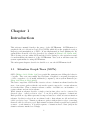
Chapter 1
Introduction
This reference manual describes the usage of the SGTEditor. SGTEditor is a
graphical editor for Situation Graph Trees (SGTs) which allows the graphical creation,
inspection and manipulation of SGTs. It was implemented in Java utilizing the Diagram Editor Generator DiaGen described for example in [Minas 1997; Minas 2001].
The following sections outline SGTs and the DiaGen package to the extend neccessary
for understanding the function of the SGTEditor. One section will then state the
system requirements for using SGTEditor.
The subsequent chapters describe in detail how to use the SGTEditor itself.
1.1
Situation Graph Trees (SGTs)
SGTs ([Krüger 1991; Schäfer 1996]) are graph–like structures modelling the behavior
of agents. They were successfully used in terms of highlevel conceptual descriptions
of video–sequences of road traffic within the (computer–) vision system Xtrack (see
[Haag 1998; Haag & Nagel 2000]).
The basic component of SGTs is the situation scheme. A situation scheme describes the
state of an agent together with the actions the agent is expected to execute whenever
it is in that state. Thus, a situation scheme consists – in addition to an identifier – of
a state scheme and an action scheme.
While situation schemes describe a single point in time, they can be connected by
directed edges – called prediction edges – to model possible sequences of situations.
Each prediction edge thus represents a temporal successor–relation between situation
schemes. Prediction edges from one scheme back to that scheme are allowed and are
called prediction loops. Situation schemes together with prediction edges connecting
them are called a situation graph. Each situation scheme in such a graph can be marked
as start– or end situation. A possible sequence of situations has to start (end) in the
situation schemes marked accordingly.
1
2
CHAPTER 1. INTRODUCTION
Each situation scheme in a graph can be connected to another situation graph by a
so–called specialization edge. This means that such a situation scheme is temporally
or conceptually further particularized by the connected situation graph. The situation
scheme is called more general than the situation graph and the situation schemes it
comprises. While the connection of one situation scheme to more than one specializing
graph is allowed, circles due to specialization edges are forbidden. Specialization edges
are used to recursively create a tree–like structure of situation schemes – contained in
situation graphs – connected to less general situation graphs.
To define SGTs, [Schäfer 1996] developed the language SIT++, in which each aspect
of an SGT can be described textually. To further use an SGT described in a SIT++–
textfile, this file is converted into a logic–format which can be evaluated by the inference
engine F–Limette, also developed by [Schäfer 1996].
1.2
DiaGen– A Diagram Editor Generator
DiaGen is a generator for powerful diagram editors and is free software under the terms
of the GNU General Public License ([GPL 1]). Editors for new diagram types can be
created with DiaGen by defining the structure of those diagram types as a hypergraph
grammar. This enables the generated editor not only to visualize diagrams, but also to
analyse the structure of those diagrams. The structure information can then be used
to layout the diagram components, to build internal data structures representing the
diagram semantics or simply to inform the user that the actual diagram (or a certain
part of it) does not conform to the desired diagram structure. The following description
of DiaGen has been taken from [DiaGen 1] (dated February 2001):
DiaGen is a system for easy developing of powerful diagram editors. It consists of two
main parts:
• A framework of Java classes that provide generic functionality for editing and
analyzing diagrams.
• A generator program that can produce Java source code for most of the functionality that depends on the concrete diagram language.
The combination of the following main features distinguishes DiaGen from other existing diagram editing/analysis systems:
• DiaGen editors include an analysis module to recognize the structure and syntactic correctness of diagrams on-line during the editing process. The structural
analysis is based on hypergraph transformations and grammars, which provide a
flexible syntactic model and allow for efficient parsing. DiaGen has been specially designed for fault-tolerant parsing and handling of diagrams that are only
partially correct.
1.3. SYSTEM REQUIREMENTS
3
• DiaGen uses the structural analysis results to provide syntactic highlighting and
an interactive automatic layout facility. The layout mechanism is based on flexible
geometric constraints and relies on an external constraint-solving engine.
• DiaGen combines free-hand editing in the manner of a drawing-program with
syntax-directed editing for major structural modifications of the diagram. The
language implementor can, therefore, easily supply powerful syntax-oriented operations to support frequent editing tasks, but she does not have to worry about
explicitly considering every editing requirement that may arise.
• DiaGen is entirely written in Java and is based on the new Java 2 SDK. It is,
therefore, platform-independent and can take full advantage of all the features
of the new Java2D graphics API: For example, DiaGen supports unrestricted
zooming, and rendering quality is adjusted automatically during user interactions.
The standard editor created by DiaGen for a SGT–hypergraph grammar (compare
A.2.2) provided the basis for the SGTEditor. Implemented extensions were mainly
concerned with layouting, certain editing functionalities, and semantic zooming. Semantic zooming describes view changes, where details of the diagram are suppressed
or restored. Thus, semantic zooming is no simple magnification of the whole diagram
but a piecewise enlargement of some details due to the suppression of other details. In
SGTEditor, semantic zooming can be performed by hiding or showing single situation
graphs and by hiding or showing state– and action–predicates of situation schemes.
The constraint–solver–based layout facilities of DiaGen were replaced completely by
a layout algorithm based on force simulation and knowledge about the structure of
SGTs.
1.3
System requirements
To use the SGTEditor, the Java SDK 2 is needed, which can be obtained from
[JAVA 1]. In addition to that, the DiaGen–package has to be installed [DiaGen 1].
Chapter 2
The SGTEditor graphical user
interface
The following sections describe the graphical user interface (GUI) of SGTEditor. It
is assumed that the user is familiar with standard operations always occuring due to
graphical interfaces.
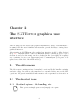
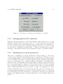
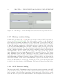
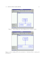
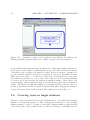
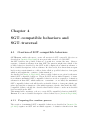
After starting the SGTEditor, the graphical user interface should look like depicted
in Fig. 2.1. The main window of the SGTEditor consists of a menu (top), two rows of
shortcut–icons (below the menu), an editor desktop (in the lower right) and a splitted
area consisting of a tree view (upper part) and a command pane (lower part of the
splitted area to the left of the main window).
2.1
The editor menu
The editor menu contains options for standard operations like file handling, printing,
and basic editing. In addition, the menu has been extended with some special SGT–
operations. All operations included in the menu are also represented as shortcut icons.
2.2
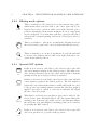
2.2.1
The shortcut icons
Standard options – file handling, etc.
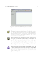
This operation simply opens a new (empty) editor pane.
New
4
2.2. THE SHORTCUT ICONS
Figure 2.1: GUI of the SGTEditor just after starting it.
Load
Save
Print
This operation opens an existing diagram. Note that this operation
can only load diagrams which were saved with the standard save–
operation. Both operations – load and save – use the standard Java
serialization of classes to export/import diagrams. This operation
can not be used to load SIT++–files.
This operation saves the diagram shown in the actually selected
editor pane. Note that this operation will not create a SIT++–file,
but will – like the open–operation described above – simply export
the Java–classes representing the diagram with standard Java–
serialization. Nevertheless, these open– and save–operations are
quite useful if the layout of the actual diagram should be saved
(temporally). SIT++ does not keep any of this layout information.
This operation will start the standard Java printing dialog. The
complete diagram of the selected editor pane will be printed. Redirection of the same diagram to be printed to a file is possible and at
the present point of implementation the only way to obtain reusable
figures of the diagrams.
5
6
CHAPTER 2. THE SGTEDITOR GRAPHICAL USER INTERFACE
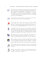
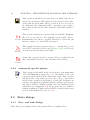
Undo
This operation revokes the last (undoable) action performed by the
user. Note that not all operations described here are undoable at
the present point of implementation. For further details on operations which are not yet undoable see Appendix 5.3. Nevertheless, the undo–operation is very useful for problems occuring due
to wrongly added or deleted components as well as for problems
related to layout insufficiencies.
This operation re–executes the last revoked operation. See the previously described undo–operation and Appendix 5.3.
Redo
Delete
Cut
Copy
Paste
ZoomIn
Zoom1
This operation deletes all selected components from the currently
selected editor pane. This operation should be undoable. Note
that due to the diagram parsing performed after the deletion of
any component, the resulting diagram does not have to be correct.
In contrast to the delete–operation, the cut–operation deletes the
currently selected components and stores them in the clipboard.
Stored components can be pasted afterwards, even in any other editor pane. Note, though, that due to diagram parsing the resulting
diagram after cutting any components does not have to be correct.
This operation stores all selected components of the current editor
pane in the clipboard, but leaves them in the editor pane, too.
Copied components can then be pasted into any other editor pane.
This operation copies any component presently in the clipboard
into the currently selected editor pane. Note that the coordinates
of any component from the clipboard will not simply be copied, but
the user will be asked to place the components at a new destination.
This operation increases the current zoom factor for the presently
selected editor pane. The current center point will be kept during
zooming.
This operation resets the zoom factor of the currently selected editor pane to a value of 1. The center point before and after the
zooming operation will be identical.
2.2. THE SHORTCUT ICONS
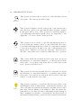
This operation decreases the zoom factor for the currently selected
editor pane. The center point will be kept.
ZoomOut
All
Cycle
Top
Bottom
Intell
This operation adjusts both the center point of the current editor
pane and its zoom factor in a way that the entire diagram contained
in this pane will be seen. This operation is extremely useful to
cope with temporally visible repaint–errors. See Appendix 5.2 and
Appendix 5.3 for more details on this problem.
This operation can be used to toggle through ambiguous user selections. If the user wants to select a component in an editor pane,
it can (and will) happen that more than one component is assigned
to the selected position. In such a case, the component first set to
that position – thus the bottom–most component – will be selected.
All other components can be reached by using this cycle–operation.
This operation lifts the presently selected component one step in
the hierarchy of components assigned to a certain position in the
editor pane. A top–most component will be reached last by the
cycle–operation described above.
This operation lowers the presently selected component one step in
the hierarchy of components assigned to a certain position in the
editor pane. A bottom–most component will be selected, if the user
clicks to a position in the editor pane.
This operation activates or deactivates the Intelligent Mode of the
SGTEditor. In the default setting – which means activated – the
editor will parse the diagram shown in the currently selected editor
pane after each modification. In addition to this, the parsed diagram will be re–layouted. Because both parsing and layout may be
time consuming, it is feasible to deactivate the Intelligent Mode for
substantial diagram editing operations and reactivate it afterwards.
7
8
CHAPTER 2. THE SGTEDITOR GRAPHICAL USER INTERFACE
2.2.2
Editing mode options
Select
This icon switches to the select mode for the current editor pane,
which means that every left–click to the editor pane will be interpreted as a select–operation, while every right–click will open a
position–dependent context–menu. In this mode, most components
are also draggable. Note that after each drag–operation, the editor
will perform a diagram parsing and layout, if Intelligent Mode is
activated.
This icon switches to pan–mode, in which the diagram shown in
the selected editor pane can be moved arbitrarily with the mouse.
Pan
Zoom
2.2.3
This icon switches to zoom–mode. In this mode each left–click will
zoom–in to the clicked position, while every right–click will zoom–
out from the clicked position.
Special SGT options
Sit
Graph
Predict
If this icon is selected, each click to the selected editor pane will
add a new situation scheme at the clicked position. Like with every
add–operation described below, the editor will perform a diagram
parsing and layout, if Intelligent Mode is activated.
If this icon is selected, each click to the selected editor pane will add
a new situation graph at the clicked position. The new situation
graph will come with default values for width and height. In order
to incorporate any existing situation scheme into this new graph it
might be necessary to switch to select–mode aftwards and adjust
the size of the new graph.
With this icon selected, new prediction edges can be added to the
selected editor pane. Each first click to the editor pane defines the
starting point of the new edge, while every second click then defines
the end point. Note that misplaced starting points can be canceled
by pressing the ESC–button.
If this icon is selected, each click to the selected editor pane will
add a new prediction loop at the clicked position.
Loop
2.2. THE SHORTCUT ICONS
Special
Attrib
ReLayout
Forces
LoadSIT
This icon switches to a mode in which new specialization edges can
be added to the selected editor pane. Like in the case of prediction
edges, each first click defines the starting point, each second click
defines the end point, and ESC again cancels misplaced starting
points.
This operation will invoke an extra dialog in which global attributes
of the SGT edited in the selected editor pane can be modified.
See Appendix A.1 for a detailed description of attributes and their
values. Although these attributes are not visible in the editor pane
itself, they will be written to the destination file, if the SGT is saved
to SIT++.
This operation does two things: first the layout algorithm is invoked for the selected editor pane again. Secondly, the tree view
of the actual diagram is created or updated. Note that any operation concerning the tree view should be preceded by one of these
redoLayout–operations.
This operation will invoke an extra dialog in which parameters of
the layout algorithm can be modified. The layout of SGT–diagrams
is based on simulated forces between situation schemes comprised
within a situation graph. The force acting between two situation
schemes can be modified by scaling the repulsion between situation nodes, the attraction between these nodes, and the minimum
(and optimal) distance which should prevail between two situation
schemes. The force simulation is performed iteratively. The maximum step number and the maximum step size can be adjusted.
The layout of situation graphs, a simple tree layout, is controlled
by the currently defined distance between two graphs.
This operation will invoke an extra dialog in which a SIT++–file can
be selected for loading. The selected SIT++–file will be parsed and
the extracted SGT will be drawn into a new editor pane. Note that
once a new SGT was loaded, the newly created diagram will first
be parsed and then the layout algorithm will be executed twice on
that diagram.
9
10
CHAPTER 2. THE SGTEDITOR GRAPHICAL USER INTERFACE
SaveSIT
Lim–Files
Histories
This operation will invoke an extra dialog in which a file can be
selected for saving the SGT depicted in the selected editor pane.
A file with the given name will be created if it does not yet exist. Otherwise, the existing file will be overwritten. As a result of
this operation, the new file will contain the saved SGT in SIT++–
notation.
This operation will invoke a separate dialog in which F–Limette–
files can be associated to the currently selected SGT. The F–
Limette–files associated to an SGT will later be loaded into the
inference–engine, e.g., if the SGT is traversed.
This operation invokes a separate dialog, too. In this dialog, maximized SGT–compatible behaviors (see [Arens & Nagel 2003]) can be
created from the currently selected SGT.
Again, this operation invokes a separate dialog, in which the the
user can start the traversal of the currently selected dialog.
Traverse
2.2.4
component–specific options
Edit
2.3
2.3.1
This operation is accessible in the lower left part of the main frame
of the SGTEditor (compare Fig. 2.1). Depending on the component presently selected in the actual editor pane, this operation
will invoke the component’s property editor. If no component is
selected, this operation is deactivated. Of all SGT diagram components, only situation graphs and situation schemes possess property editors. While for situation graphs only some attributes can be
edited there (see Apppendix A.1), the property editor for situation
schemes is much more functional and will be described in an extra
section of this manual (see section 2.3.4).
Extra dialogs
Save– and load–dialogs
These dialogs are standard Java–dialogs and will not be explained here.
2.3. EXTRA DIALOGS
11
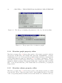
Figure 2.2: The dialog for editing global attributes of an SGT.
2.3.2
Changing global SGT–attributes
This dialog is depicted in Fig. 2.2. The dialog mainly consists of five rows of row–wise
mutually exclusive checkboxes. Each row sets one of the global attributes of the SGT
the dialog was invoked for. Each attribute has two possible values. See Appendix A.1
for a more detailed explanation of attribute meanings. The dialog can be closed with
the Ok–button, confirming all changes made, or with the Cancel–button, ignoring
all changes. The Default–button resets all attribute–values to predefined defaults.
2.3.3
Adjusting force layout parameters
The dialog for adjusting force layout parameters is depicted in Fig. 2.3. The dialog
consists of seven textfields each holding the value of one parameter. With the exception
of the maximum number of iteration steps (which is an integer value), all these parameters are floating point values. situation repulsion and situation attraction
scale the corresponding forces on situation schemes. Situation– and Graph Min–
distance denote the minimum (and optimal) distance which should prevail between
the corresponding diagram components. Max. Force on Sit. holds the maximum
step one situation scheme can make in one iteration step of the force layout algorithm.
Max. acceptable Force denotes a special force–value: if no simulated force in the
diagram reaches this value in one iteration step, the whole iteration is terminated before the maximum step number was reached. Again, this dialog can be closed pressing
the Close–button (ignoring all changes) or pressing the Ok–button (accepting all
changes). The Default–button resets all parameters to the predefined values given
in Fig. 2.3.
12
CHAPTER 2. THE SGTEDITOR GRAPHICAL USER INTERFACE
Figure 2.3: The dialog for adjusting all parameters of the force layout algorithm.
Figure 2.4: The property editor for situation graphs.
2.3.4
Situation graph property editor
This dialog (compare Fig. 2.4) shows all properties of the situation graph for which it
was invoked. In this dialog, the default value (not set, incremental, or nonincremental) can be set for action predicates inside situation schemes contained in the
corresponding situation graph (see Appendix A.1 for details on attributes). This default value is passed down from the global setting of the SGT itself to situation graphs
and then to situation schemes. The parent default value – namely the value set in the
SGT – is also shown in this dialog. The Close–button closes this dialog, accepting all
changes made.
2.3.5
Situation scheme property editor
This dialog (compare Fig. 2.5) shows all properties of the situation scheme for which
it was invoked. Most of these properties can be edited within this dialog. The name
of the corresponding situation scheme is shown and editable in a textfield at the top.
2.3. EXTRA DIALOGS
13
Figure 2.5: The property editor for situation schemes.
This textfield is followed by a table holding all state predicates of the scheme. Each
of these state predicates can be selected and edited. A single state predicate can be
deleted by selecting it and pressing the Delete–button to the right of the state–
predicates. A new state predicate can be added by simply pressing the Add–button
and typing in the new predicate string into the newly created entry of the table. This
new entry has to be confirmed by pressing Enter. The action predicates can be
handled in the same way. A table holds all predicates, Add– and Delete–button
are positioned to the right of the table. The next table shows all predictions starting
in the corresponding situation scheme. Note that new predictions can only be added
graphically, as well as predictions can only be deleted graphically. Here, only the order
of predictions as well as the binding scheme corresponding to each prediction can be
edited. The place of a single prediction can be changed by clicking to the prediction
(in the first column named Succ. Sit) and then clicking to the row in the table the
prediction is meant to be placed (The order of predictions is also indicated by small
numbers in the editor pane. This indication is updated after the situation scheme
property editor has been closed.). The binding scheme of each prediction edge can be
edited by selecting the desired binding scheme in the predictions table and then press
the Edit Binding–button. This operation starts a new dialog, which is described
in Section 2.3.5.1. The next part of the situation scheme property editor deals with
default values for action predicates inside the corresponding scheme. Again, the value
of superior components can be kept (not set), or the default can be set to one of
the possible values (incremental, nonincremental). Then, two checkboxes let the
user define the corresponding situation scheme as start– and/or end–situation. The
button Incr. State invokes a new dialog showing the incremental state scheme of the
situation scheme, which is described in Section 2.3.5.2. The button Close closes the
14
CHAPTER 2. THE SGTEDITOR GRAPHICAL USER INTERFACE
Figure 2.6: The dialog for editing a binding scheme of one prediction edge.
situation scheme property editor and all subordinated dialogs.
2.3.5.1
Binding scheme dialog
This dialog (compare Fig. 2.6) first re–displays the binding scheme it was invoked
for in form of a table. In this table, each constraint of the binding scheme occupies
one row. The order of the rows can again be modified by clicking on the row to
be moved and then clicking on the row this constraint is to be moved to. Binding
schemes comprise two different kinds of constraints: variable releases and assignments.
New binding constraints can be added by filling the corresponding textfields below
the table and then press the Add Assignment–button (the Add Release–button,
respectively). The textfields used for the new binding constraint will be reset after each
add–operation. To delete a single binding constraint, it has to be selected in the table
and the Delete Binding–button has to be pressed. The complete binding scheme
will be updated when the dialog is closed by pressing the Close–button.
2.3.5.2
Incremental state scheme dialog
This dialog is for mere inspection rather than for editing purposes. The dialog shows
all state predicates which have to become true in order to instantiate the situation
scheme the dialog was invoked for. The dialog is divided into two parts: on the left the
hierarchy of situation schemes from the root graph of the SGT down to the selected
situation scheme is shown. The state predicates of each of these situation schemes is
given in the right part of the dialog. The dialog can be closed by pressing the Close–
button, but is also closed when the superior situation scheme property editor is closed.
2.3. EXTRA DIALOGS
15
Figure 2.7: The dialog showing the incremental state scheme of one situation scheme.
Figure 2.8: The dialog to associate F–Limette–files to the currently selected SGT.
2.3.6
F–Limette–File association dialog
This dialog (compare Fig. 2.8) enables the user to associate F–Limette–files to the
SGT the dialog has been invoked for. The dialog window consists of a table (to the
left), which shows all files presently associated to the SGT, and a set of buttons (to
the right) which let the user add a single file (add File), add all files from a certain
directory (add All). Note that add File and add All will invoke standard Java
file dialogs. In the case of add File, the file dialog will accept only a single file with
the extension .lim, while in the case of add All, only directories will be accepted and
only files in that directory with the extension .lim will be added to the list. To delete
a file from the list, the file has to selected in the table and the button titled del File
has to be pressed. The button Close closes the dialog.
16
CHAPTER 2. THE SGTEDITOR GRAPHICAL USER INTERFACE
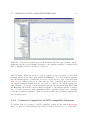
Figure 2.9: The dialog to create and inspect maximized SGT–compatible behaviors.
2.3.7
History creation dialog
In this dialog (compare Fig. 2.9), the user can create maximized SGT–compatible behaviors (see [Arens & Nagel 2003]). The dialog window consists of a list showing the
previously selected situation schemes (top left, titled Sits), an associated button to
delete single situations from that list (top center, titled del. Situation). In addition
to that, the window comprises two other tables and a set of buttons. One of the table,
(lower left, titled Histories) shows all SGT–compatible behaviors created for the list
of selected situations (Sits). The other table (lower right, titled Sits of Hist.) shows
the list of situation schemes contained in a SGT–compatible behavior selectable in the
table Histories. The two button in the center of the dialog let the user generate
(gen. History) and view (view History) SGT–compatible behaviors. The button
gen. History creates all SGT–compatible for the list of situation schemes visible
in the table Sits. If a previously created SGT–compatible behavior is selected in the
table Histories, all situation schemes contained in that behavior are shown in the
table Sits of Hist.. If the button view History is pressed, the currently selected
behavior in Histories is converted into an SGT and an editor pane showing that SGT
is added to the editor desktop of SGTEditor. The button Close closesd the dialog.
2.3.8
SGT–Traversal dialog
The dialog titled SGT–Traversal is used to start and stop the traversal of the SGT
it was invoked for and to inspect the results of that traversal (compare section 4.2 The
dialog consists of the following components: In the upper part of the dialog, a table
shows the list of trajectory–files which should be used as input for the traversal to be
2.3. EXTRA DIALOGS
17
Figure 2.10: The dialog to start SGT–traversals.
started. To the left of that table, three buttons can be used to add a single file or all
files from a directory to that table or to delete a single file from that table (compare
Section 2.3.7). Below the table of trajectory–files and associated buttons, two radio
buttons can be used to select whether the traversal should be started as simulation
(select Yes) or as situation analysis (select No). The text field in the lower part of the
dialog shows all (textual) results of the traversal. The actual traversal can be started
with the button Start and stopped with the button Stop. The button Close stops
a probably running traversal and closes the dialog.
Chapter 3
SGT–Editing – A simple example
The following section demonstrates the graphical construction of a new SGT with the
SGTEditor. However, all aspects and techniques decribed in the following sections
apply, too, for SGTs loaded from SIT++ sources for modification. For all references on
GUI components (like shortcut icons), the following sections will point to the previous
chapter.
Note that all screenshots visualizing SGTEditor–details in the following where created with an older version (v1.0) of SGTEditor. Nevertheless, all steps to create and
visualize an SGT described in the following are still applicable in the present version
of SGTEditor.
3.1
Starting from scratch
The first step is to start the SGTEditor. Into the empty editor pane – named
Untitled – in the lower right editor desktop (compare Fig. 2.1), new SGT components
can already be added. It is recommended to maximize this editor pane inside the editor
desktop.
3.2
Adding new components
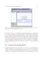
To add new components, select one of the shortcut icons Sit, Graph, Predict, Loop
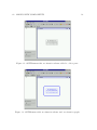
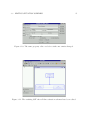
or Special. We will start here by adding a new situation scheme by selecting Sit and
then clicking somewere into the editor pane. The result of this action can be seen
in Fig. 3.1: the added situation scheme is depicted in black at this stage. We will
now add a new situation graph (frame) to the editor pane by selecting Graph and
then click more or less exactly to the center of the previously added situation scheme
(compare Fig. 3.2). Note that now both the situation scheme and the situation–
graph turned to blue color. The SGTEditor indicates thereby that the diagram
18
3.2. ADDING NEW COMPONENTS
Figure 3.1: SGTEditor with one situation scheme added to editor pane.
Figure 3.2: SGTEditor with one situation scheme and one situation graph.
19
20
CHAPTER 3. SGT–EDITING – A SIMPLE EXAMPLE
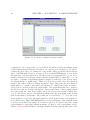
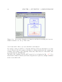
Figure 3.3: Some more situation schemes added.
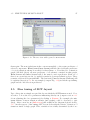
constructed so far corresponds to a correct SGT. We will now add a specializing graph
for the existing situation scheme. We first zoom out (ZoomOut), therefore, in order to
obtain some more space for adding new components. Then, we disable the Intelligent
Mode of SGTEditor (Intell), because we do not want SGTEditor to re–layout the
diagram after each user–interaction. We then select Sit again and add, e.g., two more
situation schemes below the previously constructed simple SGT (compare Fig. 3.3). As
we want to construct a specializing situation graph, we will need to incorporate these
two situations into a graph frame. Thus, we select Graph and add a new situation
graph to the center of the two situation schemes. Up to this point, the new situation
graph will be too small to surround both schemes. To enlarge the graph, we turn to
Select mode and select the new graph frame. The graph will turn red to indicate
the selection and two handles will appear. One (in the center of thew graph) lets us
move the graph, the other (lower right corner) lets us resize the graph (compare Fig.
3.4). To incorporate the two new situation schemes into the new graph, resize it such
that it surrounds both schemes. The result can be seen in Fig. 3.5. Now, the lower
(new) graph is colored blue, the upper turned to black again because both graphs are
not connected yet. Thus, SGTEditor has to decide which part of the diagram it has
to declare as an SGT and which one should be ignored. To declare the lower graph
as specialization of the upper situation scheme, we have to add a specialization edge.
Click to Special and then first to the upper situation scheme (start point), then to the
3.2. ADDING NEW COMPONENTS
21
Figure 3.4: To resize a graph, select it and move the handle in the lower right corner.
Figure 3.5: SGTEditor decides to declare lower graph as SGT.
22
CHAPTER 3. SGT–EDITING – A SIMPLE EXAMPLE
Figure 3.6: Now both graphs build one single SGT.
lower situation graph (end point). Now, both graphs turn blue because they are both
part of the (now connected) SGT. We want the two situation schemes to be connected
by a prediction edge. In addition, we want each situation scheme in the graph to be
self–predicting, i.e. connected to itself by a prediction edge. We first click to Predict,
then define start– and end–point of the new prediction edge by clicking first to the left,
then to the right lower situation scheme. Then we select Loop, and click once to each
situation scheme of the SGT. Note that up to this point, no layout is done for the SGT.
As a result, each and every edge starts and ends wherever it was set (compare Fig.
3.7. To let SGTEditor update the layout of the new SGT, reactivate the Intelligent
Mode (Intell). Then click to All once, to center and maximize the SGT diagram.
The result is depicted in Fig. 3.8.
So far, we just built up the structure of an SGT consisting of situation schemes, graphs
and edges. All situation schemes are named the same (ED UNDEFINED SIT) and
no scheme contains any state– or action–predicates. Also the numbers given to edges
presently just represent the order in which edges have been added. The next steps will
edit the situation schemes themselves and reorder some prediction edges.
3.2. ADDING NEW COMPONENTS
23
Figure 3.7: After adding some edges, things get more and more messy.
Figure 3.8: The resulting SGT after reractivation of Intelligent Mode, centering and
maximization.
24
CHAPTER 3. SGT–EDITING – A SIMPLE EXAMPLE
Figure 3.9: The property editor for the top–most situation scheme.
3.3
Editing situation schemes
To edit a situation scheme, switch to Select mode. After selecting the situation
scheme to be edited, you can either right–click to that scheme again: this will show a
context–menu in which the item show Properties will invoke the situation scheme
property editor1 . Alternatively, this editor can be invoked by clicking to the Edit
icon in the lower left control panel. We will start the property editor for the top–
most situation scheme first (compare Fig. 3.9). First we change the name of that
situation scheme, e.g., to Editing SGTs. Then we add a state predicate as described
in section 2.3.4, for example active(User). The action scheme of this situation should
only consist of a predicate which prints a string, let’s say “The user is active.”, to the
output stream. So we add note(“The user is active.”) as action predicate. We
want this scheme to be both a start– and an end–situation, so we select both checkboxes
(compare Fig. 3.10). Then this dialog is closed by pressing Close. After having closed
the dialog, the new entries for the top–most situation scheme should have been updated
in the editor pane. If not, try to redraw the diagram by clicking to All, or even force
SGTEditor to relayout the diagram clicking to Intell and then to All. After
editing the properties of the other two situation schemes, the result might look like
depicted in Fig. 3.11. Note that we also reordered the prediction edges of the lower–
left situation scheme as described in section 2.3.5. In the way described above, more
and more complex SGTs can be created. First, the structure is extended by disabling
the Intelligent Mode (Intell) and adding components. Then, after reactivation of the
Intelligent Mode, detailed properties of single components can be edited.
1
Note that on some systems this right–click on components might have no effect at all. This
problem arises due to different handling of so–called popup triggers on, e.g., Linux XServers and
Windows. See also Appendix 5.2 for more details regarding this problem.
3.3. EDITING SITUATION SCHEMES
25
Figure 3.10: The same property editor as before with some entries changed.
Figure 3.11: The resulting SGT after all three situation schemes have been edited.
26
CHAPTER 3. SGT–EDITING – A SIMPLE EXAMPLE
Figure 3.12: The tree view of the SGT was created and is depicted in the tree view
panel (top–left of frame).
3.4
Semantic zooming
Although the semantic zooming options were implemented to cope with huge SGTs,
they will be demonstrated at the simple SGT created above. To execute any of the
semantic zooming operations, first the tree view for the presently edited SGT has to
be created. This can be done by clicking to the ReLayout icon. The tree view
created by this action is then shown in the tree view panel (top–left of SGTEditor,
compare Fig. 3.12). Each entry in this tree corresponds to a component of the SGT
it was created for. Upon left–clicking to an entry, the corresponding component in
the editor pane will be selected. When right–clicking to an entry, a context–menu
will be shown (compare Fig. 3.13). The first two items in this context menu relate
to the tree view itself: Expand Subtree will expand all children from the selected
component downwards, while Fold SubTree will fold all those children. The next
two items – Hide and Show – will hide or show, respectively, components in the
editor pane. If the context–menu was invoked for a situation scheme, the Hide–
operation will hide all situation graphs specializing this situation scheme together with
all graphs subordinated to these graphs. The Show–operation will show all these
graphs again. Invoked for a situation graph, the Hide–operation will hide only this
situation graph together with all subordinated graphs, the Show–operation will show
3.5. FINE TUNING OF SGT–LAYOUT
27
Figure 3.13: The tree view with opened context–menu.
them again. The next eight items in the context–menu hide or show state predicates of
selected components. Hide State (Show State) will hide (show) all state predicates
of a single situation scheme if executed for that scheme or, if executed for a situation
graph, will hide (show) all state predicates of all schemes contained in that graph.
Hide Action and Show Action will do the same for action predicates. Each one of
these four operations can also be applied recursively down specialization edges. These
recursive versions all begin with Rec.. The last item (View in Single Window) will
be explained in section 3.6. In our example (compare Fig. 3.14) we hid the specializing
graph and also hid all action predicates.
3.5
Fine tuning of SGT–layout
Up to this point we simply accepted the layout which the SGTEditor created. Now,
we take a look at the force parameters influencing this layout (compare section 2.3.3
about adjusting the force parameters) by clicking to Forces. For example, the minimum distance between situation schemes (and graphs) could be decreased to 80.0
(10.0). After a new layout (ReLayout) this results in the diagram depicted in Fig.
3.15. Another aspect of fine tuning SGT–layout deals with the relative orientation of
situations inside a single graph. This orientation is not fully determined by the force
28
CHAPTER 3. SGT–EDITING – A SIMPLE EXAMPLE
Figure 3.14: Semantic zooming: action predicates were hidden. In addition, the
hidden specializing graph is indicated by a filled rectangle below the situation.
layout, which mainly guarantees that no situations overlap, that situation schemes are
positioned in a user–defined optimal distance from each other and that the number
of prediction edge crossings is as small as possible. However, the mere orientation of,
e.g, two situation schemes connected by a prediction edge is not determined by this.
Thus, the layout of Fig. 3.15 could also be altered in a way that the two lower situation schemes are stacked one on top of the other. This can be done by first switching
to Select mode and selecting the right–most situation scheme. Then, click to the
centered handle of that scheme and drag it beneath the previously left–most situation
scheme. The situation graph surrounding both schemes and the prediction edge connecting both schemes should be updated automatically while dragging the situation,
because Intelligent Mode is still activated. The result can be seen in Fig. 3.16.
3.6
Creating views in single windows
The last operation described here was also implemented to cope with huge diagrams,
mainly for documentation purposes. This operation allows the user to select a single
situation graph to be the root graph of a new SGT–diagram, which is depicted inside
a new editor pane. This operation can be reached by creating or actualizing the tree
3.7. SAVING AND RELOADING SGTS
29
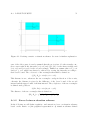
Figure 3.15: Layout after adjusting some force parameters Compare Fig. 3.12 for this
graph layouted with default parameter values.
view with ReLayout. To view a situation graph in a single window, select this graph
in the tree view panel and open the context–menu by right–clicking on that graph.
Now, select the item View in Single Window. As a result, a new editor pane opens
inside the editor desktop which should only contain the selected graph (as root) and all
situation graphs subordinated to the selected graph. Thus, a diagram of a sub–SGT
was created. Note that this operation is only for documentation purposes at the present
point of implementation (the new editor pane, therefore, is marked as CLIPPING:
Only for viewing !). Editing operations done in this editor pane can only affect
the layout within this pane, but will not affect the original SGT or the corresponding
diagram.
3.7
Saving and reloading SGTs
The SGT created above can be saved either as a SIT++ file or it can be saved as a
diagram. The first option creates files which can be edited easily with a text editor
and can be further converted into logic programs (compare [Schäfer 1996]). SIT++ files
can also be reloaded into the SGTEditor, however, with one drawback: the layout
of the SGT – automatically created by SGTEditor or adjusted by the user – will be
30
CHAPTER 3. SGT–EDITING – A SIMPLE EXAMPLE
Figure 3.16: Layout after dragging one situation and thereby stacking the lower two
situation schemes one on top of the other.
lost because SIT++ files do not save this kind of information.
In contrast, saving an SGT as a diagram will keep all layout information for later
reload. However, the file format created here is binary (namely the file contains the
serialized Java classes of the diagram). Thus, those files cannot be edited with other
programs than the SGTEditor.
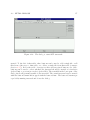
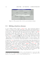
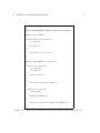
The SIT++ file resulting from the SGT created above is depicted in Fig. 3.17. Note
that situation names formerly used in the diagram were replaced by unique identifiers
in the created SIT++ file.
3.7. SAVING AND RELOADING SGTS
// automatically generated by SGTEditor.
//
DEFAULT NONINCREMENTAL GREEDY PLURAL DEPTH TRAVERSAL;
GRAPH gr_ED_SITGRAPH0
{
START FINAL SIT sit_ED_SIT0 :
sit_ED_SIT0
{
active(User);
}
{
note("The user is active.");
}
}
GRAPH gr_ED_SITGRAPH1 : sit_ED_SIT0
{
START SIT sit_ED_SIT1 :
sit_ED_SIT1,
sit_ED_SIT2
{
read(User,manual);
}
{
note("User presently learning.");
}
FINAL SIT sit_ED_SIT2 :
sit_ED_SIT2
{
using(User,SGTEditor);
}
{
note("User presently working with SGTEditor");
}
}
Figure 3.17: SIT++ file resulting from the SGT created in the sections above.
31
Chapter 4
SGT–compatible behaviors and
SGT–traversal
4.1
Creation of SGT–compatible behaviors
SGTEditor enables the user to create all maximized SGT–compatible behaviors as
described in [Arens & Nagel 2003] from a previously created or loaded SGT.
An SGT describes the possible behaviors of agents in a certain discourse. Given a
sequence of situation schemes from that SGT, the question might arise which of the
possible behaviors described by the SGT would comprise those situation schemes or
more detailed descriptions of those schemes. In other words, if we knew that an agent
has been in a certain situation, could we derive all those possible behaviors of an agent,
which would explain the occurence of that situation ?
As described in [Arens & Nagel 2003], these possible behaviors are given by the maximized SGT–compatible behaviors. Given an SGT and an initial sequence of situation schemes, maximized SGT–compatible behaviors are those sequences of situation
schemes from that SGT, which satisfy two constraints: on one hand, the maximized
SGT–compatible behavior should describe an feasible behavior of an agent, which comprises (at least) those situations of the initial sequences. On the other hand, the SGT–
compatible behavior should also describe that feasible behavior on the most detailed
level accessible in the SGT.
This manual will concentrate on how to create SGT–compatible behaviors with SGTEditor. For a more detailed description of those behaviors, see [Arens & Nagel 2003].
4.1.1
Preparing the creation–process
The creation of maximized SGT–compatible behaviors as described in [Arens & Nagel 2003] requires an SGT and an initial sequence of situation schemes from that
32
4.1. CREATION OF SGT–COMPATIBLE BEHAVIORS
33
Figure 4.1: The tree view with opened context–menu. The last option in that context–
menu will add the selected situation scheme to the present sequences of situations an
SGT–compatible behavior should be created for.
SGT as input. Thus the creation of those behaviors can be started for any SGT
presently shown in an editor pane within SGTEditor. To select situation schemes
into the initial sequence of situations, we need to create the tree–view of the SGT with
ReLayout (compare section 3.4). Once the tree view of the SGT has been created,
any situation scheme within this tree view can be added to the initial sequence by
right–clicking to it. In the context–menu showing up, the last menu item titled Add
to History will add the selected situation scheme to the initial sequence (compare
Fig. 4.1). The next step towards maximized SGT–compatibe behaviors is to actually
create those situation sequences. This is done in an extra dialog, which is explained in
the following section.
4.1.2
Creation & inspection of SGT–compatible behaviors
To call the dialog for creation of SGT–compatible behaviors, the button Histories
has to be pressed. This will show the dialog described in section 2.3.7. Any SGT–
34
CHAPTER 4. SGT–COMPATIBLE BEHAVIORS AND SGT–TRAVERSAL
Figure 4.2: One maximized SGT–compatible behavior as SGT. The upper situation
graph consists of a default situation scheme without any state or action predicates. This
scheme is particularized by another graph, which contains the sequence of situations
of the created behavior.
compatible behavior created there can be viewed as an SGT itself. An SGT–compatible
behavior is converted into an SGT in the following way: the behavior consists of a
sequence of situations. This sequence of situations is added to a situation graph,
marking the first situation as start situation and the last one as end situation. Note
that the state scheme and action scheme of the situation schemes added to the new
graph represent the incremental state and action schemes of the original situations.
Prediction edges between two consecutive situations are copied from the initial SGT
the behavior was created for. If no prediction edge between two consecutive situations
of the sequence was present in the SGT, those prediction edges from the SGT are
copied, which – going from those schemes upwards towards the root graph of the
SGT – first connect a parent situation of the first scheme to a parent situation of the
second scheme. Self predictions are added to any situation of the sequence, which also
obtained a self prediction in the initial SGT. The situation graph created in this way
is connected to a general situation with no state scheme and no action scheme. This
general situation is added to a second graph, which constitutes the root graph of the
4.2. SGT–TRAVERSAL
35
new SGT. The created SGT is inserted into a new editor pane and added to the editor
desktop (compare Fig. 4.2).
4.2
SGT–traversal
SGT–traversal means to run through an SGT along prediction and specialization edges.
SGT–traversal can be performed for two different purposes: on one hand, the user
might want to feed in vision results obtained from a video sequence and might want
to know which situation scheme is instantiated by which agent extracted by the vision
system, i.e., for which situation can all state predicates be satisfied. Thus, the traversal
is performed as an situation analysis: for the first point in time observed, a start
situation in the root graph of the SGT is searched which can be instantiated for a
certain agent. From this scheme on, a most special scheme is searched for the same
time point, walking along specialization edges to specializing graphs, in which only
start situations are invesitgated. If a most special situation was found for the present
time point, only those situation schemes will be investigated for the next time point,
which are connected by prediction edges (or loops) to that last scheme, and so on.
Thus, the traversal tries to predict on the same level of detail and tries to find the
most detailed description for that prediction. If such a prediction fails, the traversal
might also generalize to a parent scheme again, but only if the last scheme instantiated
on the more detailed level was marked as an end–situation. The situation analysis
results in a sequence of instantiated situation schemes for each agent extracted by the
vision system. For a more detailed description of SGT–traversal in the sense described
above, see [Haag & Nagel 2000] and [Schäfer 1996].
The other purpose of SGT–traversal is to generate video sequences. While in the case of
situation analysis, vision results were fed in to test for the satisfaction of state predicates
of situation schemes, the generation task produces a ground truth by traversing an
SGT and executing all action predicates of situation schemes it instantiates during
that traversal. Starting with an initial state of the discourse in question, the traversal
again searches for a most special situation scheme it can instantiate for that world–
state. But the state for the next time point is not included – as in the situation analysis
– as vision results, but is created by the execution of action predicates associated to
the situation scheme instantiated last. Thus, each situation scheme instantiation leads
to the execution of certain actions defined in that scheme. These actions alter the
world state and result in a new world state, which then is used to instantiate the next
situation scheme and so on.
The difference between both kinds of SGT–traversals mentioned above visually only
appears in the creation of result files in the latter case. In this generation task the
traversal finishes by stating in which files the world states created during traversal have
been saved. Internally, both kinds of SGT–traversals are performed by translating the
SGT in question into a logic formulation, which can be imported by the inference engine
36
CHAPTER 4. SGT–COMPATIBLE BEHAVIORS AND SGT–TRAVERSAL
F–Limette. The vision results (in case of a situation analysis) or the initial world
states (in case of the generation task) are also included into that inference engine. To
link vision results or initial world states to the state and action predicates mentioned
in the situation schemes of the SGT, it might be (and normally is) necessary to define
a terminology again in form of logic programs includable into F–Limette.
Thus, the SGT–traversal with SGTEditor is normally preceded by defining the files
containing this terminology (compare section 2.3.6). As each SGT might make use of
different terms defined in different terminology files, these files have to be defined for
each SGT separately. Note, however, that maximized SGT–compatible behaviors in
form of SGTs inhere the terminology files of the SGT they were created for.
To summarize the necessary steps for SGT–traversal: first an SGT to be traversed
should be loaded or created in an editor pane. Then, the terminology files containing
the explaination of state and action predicates should be defined using the button
Lim–Files and the dialog explained in section 2.3.6. After that, the traversal dialog
(explained in section 2.3.8) should be opened using the button Traverse. In this
dialog, the files containing vision results or initial world states can be defined (see
section 2.3.8). After declaring the kind of SGT–traversal to be run by SGTEditor,
the traversal can be started and the results can be viewed again in the dialog described
in section 2.3.8.
4.2.1
Viewing results of SGT–traversal in case of generation
tasks
In the generation task, i.e., in creating world states during SGT–traversal, it normally
is not satisfiable to just view a textual representation of these world states. Because
the traversed SGT had been created for a discourse viewable for a vision system, the
user might want to get an idea of how that – probably changing – discourse might
have looked like for that vision system if it had comprised the states created during
SGT–traversal. In other words, the created world states are much easier to inspect if
they are visualized as images of the world in question.
The actual implementation of the visualization of world states depends of course on the
discourse in question. In the case of SGTs defined for road traffic (compare section 1.1),
world states created during SGT–traversal can simply be stored in socalled trajectory–
files of road vehicles as they are also created by the vision system Xtrack itself.
Xtrack then can import these trajectory–files as if they had been created during a
vision task and can be inspected within that vision system.
Chapter 5
History, Known Bugs & Possible
Future Features
5.1
History
v1.0 The version v1.0 is the first official version of SGTEditor.
v1.1 SGTEditor was extended by functionalities for the creation of maximized SGT–
compatible behaviors (see [Arens & Nagel 2003]). In addition to that, SGTEditor was directly connected to components which facilitate the traversal of SGTs
with the inference–engine F–Limette.
v1.2 Some minor errors were removed from SGTEditor. This included one error
in the tree–like layout of situation graphs. The layout algorithm for situation
graphs was modified such that the diagram of an SGT stays more or less at the
same area of the editor pane. Thus, the nerving jump of an SGT within the
editor pane is no longer existent. In addition to that, situation schemes are now
shown as colored rectangles. This on the one hand leads to diagrams which are
easier to understand. On the other hand, the coloring of situation schemes can
be used in the future to indicate present instantiations of situation schemes. Last
but not least an error in the generation of SGT–compatible behaviors – which
led to duplicate behaviors – was removed.
5.2
Bugs
The following list contains some errors and shortcomings of the present SGTEditor–
version.
1. Insufficient error handling: Presently, all warnings, errors and other messages
of SGTEditor are prompted at the system shell from which the program was
37
38
CHAPTER 5. HISTORY, BUGS & FUTURE FEATURES
started. It might be advantageous to incorporate these messages into the GUI of
SGTEditor.
2. Redo/Undo-Problems: Several operations mainly concerning semantic zooming are not integrated into the action–history of SGTEditor. This history
enables the program to undo user actions, but also to redo those actions previously taken back by the user. Future program versions might probably get rid of
this problem.
3. Awkward context–menues: The context–menues in SGTEditor are invoked
by so–called popup triggers. The decision whether or not a certain user action is a
popup trigger is made by the system on which SGTEditor currently operates.
Unfortunately, different systems make different decisions with respect to this
point. For example – speaking about right mouse clicks as popup triggers –
Linux XServers define the pressing of the right mouse button as trigger, while
Windows defines the release of the right mouse button as trigger. As far as
extensions of the classes generated by DiaGen were concerned, these differences
were taken into account. There seems to be one class of the DiaGen package itself
(diagen.editor.ui.IdleState, to be exact) which ignores these differences, though.
Thus, on Windows machines, context–menues for diagram components might
not be reachable by right–clicking to the component. In these cases, please use
the Edit button to edit the component or any other shortcut icon for other
operations.
5.3
Possible Future Features
First, all of the errors and shortcomings mentioned in the previous section should
be eliminated. In addition to this, there are some features which a future version of
SGTEditor might probably incorporate:
1. Graphical indication of situation instantiation: The coloring of situations
schemes introduced in version 1.2 of SGTEditor might enable a graphical indication of situation scheme instantiation in the future.
2. Syntax checking: The action–predicates and state–predicates entered into situation schemes are not further investigated by SGTEditor, but are simply
stored. Syntax errors in these predicates thus do not appear until the SGT is
converted into logic and used further. Future versions of SGTEditor might
analyse the user’s input for correctness in this sense.
3. Consistency checking: The incremental state scheme of situations (compare
section 2.3.5.2) is not checked for consistency in the present version of SGTEditor. Consistency in this context means that state predicates in more special
5.3. POSSIBLE FUTURE FEATURES
39
situation schemes do not contradict state predicates in more general schemes, for
example. It is not clear presently, if such a check can be performed on the mere
predicate strings or even with the help of an underlying inference engine. Future
versions of SGTEditor might incorporate such kinds of checks, though.
4. Completeness checking: An SGT normally tries to represent the possible
behavior of an agent in a certain discourse. Although this discourse might be
very restricted, the SGT should nevertheless represent all eventualities in that
restricted discourse. For example, one situation of an SGT might be specialized into two sub–cases, according to one predicate which might hold or not.
Thus, a very common question in the construction of an SGT is: “What happens
if this predicate does not hold ?”. SGTEditor might probably indicate such
alternatives to the user. Further checks for completeness might be possible, if
SGTEditor was connected to other knowledge sources such as terminologies.
40
CHAPTER 5. HISTORY, BUGS & FUTURE FEATURES
Appendix A
Technical Annex
A.1
A.1.1
Global and local attributes of SGTs
Global attributes
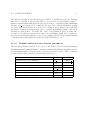
SGTs as introduced by [Schäfer 1996] have certain global attributes, which mainly
control the automatic translation of a SIT++-formulated SGT into a logic program
(compare Table A.1). These attributes can also be inspected and edited with SGTEditor, though future versions of SIT++–to–logic conversion might ignore some of these
attributes. All global attributes are stored inside a SIT++–file following the reserved
word DEFAULT. The most important attribute concerns the default incrementality
of action predicates inside situation schemes. This attribute can be overridden by local
attributes inside situation graphs, inside situation schemes or even for every single
action predicate. The other global attributes only affect the translation of a SIT++–file
into logic: search–strategy for example controls whether a situation analysis on the SGT
should be done in breadth–first– or depth–first–search. See [Schäfer 1996] for a detailed
Attribute
1. value
2. value
action–incrementality
evaluation–strategy
search–strategy
evaluation–number
evaluation–kind
NONINCREMENTAL
GREEDY
DEPTH
PLURAL
TRAVERSAL
INCREMENTAL
NONGREEDY
BREADTH
SINGULAR
OCCURENCE
Table A.1: Global attributes of SGTs and their possible values. The default value for
each global attribute is underlined.
41
42
APPENDIX A. TECHNICAL ANNEX
explanation of global SGT–attributes concerning the SIT++–to–logic conversion.
A.1.2
Local attributes
The value of the global attribute action–incrementality of an SGT can be overridden by
more local settings for this attribute. The attribute defines wether action–predicates
should be executed incrementally (everytime the corresponding situation scheme can
be instantiated) or nonincrementally (only if the corresponding situation scheme is the
most special scheme that can presently be instantiated). Thus, a global value of NONINCREMENTAL sets all action predicates to nonincremental execution. However,
the same attribute can locally be set for a situation graph to INCREMENTAL. By
this, all action predicates of situation schemes inside that graph will be set to incremental execution. Again, the value can be set even more locally for situation schemes or
even single action predicates and thus let the user define the incrementality of actions
in a very detailed way.
A.2
A.2.1
Some Grammars
SIT++–Grammar
The SIT++ grammar used for SGTEditor is documented below. In comparison to
[Schäfer 1996], those parts of SIT++ files describing a terminology (formerly introduced
by TERM) and those parts describing additional data in form of facts (formerly introduced by DATA) are not supported anymore. These parts are believed to be better
defined in other terms of knowledge representations than in the SGT–describing format.
Note also that no minimum durations for situation instantiation and no minimum
acceptable truth values for state predicates can be defined with SIT++ files conforming
the grammar below.
And a last point to be mentioned here is that the implicit typing of variables is forbidden
now. This implicit typing allowed, for example, state predicate like drive on(Agent,
lane : L), which was interpreted as two predicates, namly the original one (driveon(Agent,L)) and an additional predicate stating that the variable L is of type lane
(thus, lane(L)). The two constraints expressed by the former one predicate have to be
coded into two predicates directly now.
START
global attributes
−→
−→
global_attributes sit_graph_list
P_DEFAULT
( (<P_INCREMENTAL> | <P_NONINCREMENTAL>)
(<P_GREEDY>
| <P_NONGREEDY>
)
(<P_DEPTH>
| <P_BREADTH>
)
(<P_PLURAL>
| <P_SINGULAR>
)
A.2. SOME GRAMMARS
sit graph list
sit graph
−→
−→
graph attr
graph name
super list
sit list
situation
−→
−→
−→
−→
−→
sit attr
−→
prediction list
−→
sit name
bind list
binding
state
action
relation
−→
−→
−→
−→
−→
−→
infix relation
arg list
−→
−→
procedure
−→
individual
−→
<WHITE SPACE>
−→
43
(<P_TRAVERSAL>
| <P_OCCURRENCE>
)
)*
<P_SEMICOLON>
(sit_graph)*
graph_attr <P_GRAPH> graph_name
( <P_COLON> super_list
<P_OPEN_BRACE> sit_list <P_CLOSE_BRACE>
) |
<P_OPEN_BRACE> sit_list <P_CLOSE_BRACE>
<P_INCREMENTAL> | <P_NONINCREMENTAL>
<P_IDENTIFIER>
sit_name <P_COMMA> (sit_name)*
(situation)*
sit_attr <P_SIT> sit_name
( <P_COLON> prediction_list
<P_OPEN_BRACE> state <P_CLOSE_BRACE>
<P_OPEN_BRACE> action <P_CLOSE_BRACE>
) |
( <P_OPEN_BRACE> state <P_CLOSE_BRACE>
<P_OPEN_BRACE> action <P_CLOSE_BRACE>
)
( <P_START>
|
<P_FINAL>
|
<P_INCREMENTAL>
|
<P_NONINCREMENTAL>
)*
sit_name
[<P_OPEN_ROUND_BRACE> bind_list <P_CLOSE_ROUND_BRACE>]
( <P_COMMA> sit_name
[<P_OPEN_ROUND_BRACE> bind_list <P_CLOSE_ROUND_BRACE>]
)*
<P_IDENTIFIER>
binding (<P_COMMA> binding)*
(<P_VARIABLE> <P_ASSIGN> <P_VARIABLE>) | <P_VARIABLE>
(relation <P_SEMICOLON>)*
(procedure <P_SEMICOLON>)*
( <P_IDENTIFIER>
[<P_OPEN_ROUND_BRACE> arg_list <P_CLOSE_ROUND_BRACE>]
) |
infix_relation
<P_VARIABLE> <P_INFIX_RELATION> <P_VARIABLE>
(<P_VARIABLE> | individual)
(<P_COMMA> (<P_VARIABLE> | individual))*
[<P_INCREMENTAL> | <P_NONINCREMENTAL>]
<P_IDENTIFIER>
[<P_OPEN_ROUND_BRACE> arg_list <P_CLOSE_ROUND_BRACE>]
( relation
|
<P_IDENTIFIER> |
<P_QUOTATION> |
<P_INTEGER>
|
<P_FLOAT>
|
<P_STRING>
)
" " | "\t" | "\n" | "\r" | "\f"
44
APPENDIX A. TECHNICAL ANNEX
A.2.2
<SINGLE LINE COMMENT>
−→
<MULTI LINE COMMENT>
−→
























<#P SMALL CHAR>
<#P CAPITAL CHAR>
<#P DIGIT>
<#P ANY CHAR>
<#P CHARACTER>








−→
−→
−→
−→
−→
−→
−→
−→
−→
−→
−→
−→
−→
−→
−→
−→
−→
−→
−→
−→
−→
−→
−→
−→
−→
−→
−→
−→
−→
−→
−→
−→
−→
−→
−→
−→
−→
"//" ( ["\n","\r"])*
("\n"|"\r"|"\r\n")
"/*" ( ["*"])* "*"
("*" | ( ["*","/"] ( ["*"])* "*"))* "/"
"GRAPH"
"SIT"
"DEFAULT"
"INCREMENTAL"
"NONINCREMENTAL"
"GREEDY"
"NONGREEDY"
"PLURAL"
"SINGULAR"
"BREADTH"
"DEPTH"
"TRAVERSAL"
"OCCURRENCE"
"START"
"FINAL"
":="
"<>" | "<" | ">" "=="
":"
";"
","
"{"
"}"
"("
")"
["\u0061"-"\u007a"]
["\u0041"-"\u005a"]
["\u0030"-"\u0039"]
["\u0021"-"\u007e"]
 | | | " "
["+","-"]
 ()*
 
 "." 
 ()*
 ()*
"’" ( ["""])* "’"
""" ( ["’"])* """
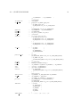
Hypergraph grammar of SGT–Diagrams
The following hypergraph grammar was formulated to define the structure of correct
SGT–diagrams to DiaGen. This definition is used by the DiaGen package to construct
Java classes which then build the basis for SGTEditor. The grammar–file consists
of six sections:
• The first section, – titled Components – defines all components which may
constitute an SGT–diagram. Most of these components directly result in Java
A.2. SOME GRAMMARS
45
classes representing the corresponding component.
• The section Relations defines all basic relations between components, e.g., that
an end–point of an edge lies within a situation scheme or graph. Although these
relations are not visible in the SGT–diagrams (as components are), they also
result in Java classes defining whether or not they should hold in a particular
case.
• Terminals defines all terminal symbols used for the definition of the hypergraph
grammar. Each terminal can have certain attributes, e.g., a terminal which
represents a prediction edge will hold two references on situation schemes.
• The section NonTerminals defines all other intermediate non–terminals used
by the hypergraph grammar. Non–terminals can have attributes, too. For example, a non–terminal representing an entire situation graph will have an entry
which holds a list of situation schemes contained in that graph.
• The Reducer defines the mapping from components and relations onto terminals
of the grammar. For example, only those situation scheme components will be
considered as terminals for situation schemes, which also lie inside a situation
graph component. Thus, the reducer section defines which basic constellations
of components are desired and which are not.
• The section Grammar defines the hypergraph grammar for SGT–diagrams itself.
While Reducer defined more local attributes of SGT–diagrams, this section
defines how situation schemes aggregate to graphs and graphs aggregate to an
SGT. Note that this grammar is basically a context–free grammar, with two
exceptions: the last two productions of this grammar are called embeddings (see
also [Minas 2001]). By these special productions, the expressiveness of grammars
for DiaGen is much more powerful than simple context–free grammars.
package SIT;
//////////////////////////////////////////////////////////////
// Components
//////////////////////////////////////////////////////////////
component
situation_scheme[1] {
Ed_SituationScheme [
Ed_SituationSchemeArea
]
};
component
situation_graph_frame[1] {
Ed_SituationGraph [
Ed_SituationGraphArea
]
};
component
prediction_edge[2] {
Ed_PredictionEdge [
Ed_PredEdgeStart,
Ed_PredEdgeEnd
46
APPENDIX A. TECHNICAL ANNEX
]
};
component
prediction_loop[2] {
Ed_PredictionLoop [
Ed_PredEdgeStart,
Ed_PredEdgeEnd
]
};
component
specialization_edge[2] {
Ed_SpecializationEdge [
Ed_SpecEdgeStart,
Ed_SpecEdgeEnd
]
};
component
pseudo[1] {
Ed_SGTRoot[
Foo
]
};
//////////////////////////////////////////////////////////////
// Relations
//////////////////////////////////////////////////////////////
relation
situation_scheme_inside_situation_graph_frame[2] {
Ed_SituationInsideGraph [
Ed_SituationSchemeArea,
Ed_SituationGraphArea
]
};
relation
prediction_edge_starts_inside_situation_scheme[2] {
Ed_PredEdgeStartsInsideSituationScheme
Ed_PredEdgeStart,
Ed_SituationSchemeArea
]
};
[
relation
prediction_edge_ends_inside_situation_scheme[2] {
Ed_PredEdgeEndsInsideSituationScheme [
Ed_PredEdgeEnd,
Ed_SituationSchemeArea
]
};
relation
specialization_edge_starts_inside_situation_scheme[2] {
Ed_SpecEdgeStartsInsideScheme [
Ed_SpecEdgeStart,
Ed_SituationSchemeArea
]
};
relation
specialization_edge_ends_inside_situation_graph_frame[2] {
Ed_SpecEdgeEndsInsideScheme [
Ed_SpecEdgeEnd,
Ed_SituationGraphArea
]
};
//////////////////////////////////////////////////////////////
// Terminals
A.2. SOME GRAMMARS
//////////////////////////////////////////////////////////////
terminal
T_situation_scheme[2] {
Ed_SituationScheme scheme;
Ed_SituationGraph graph;
};
terminal
T_prediction_edge[2] {
Ed_PredictionEdge edge;
Ed_SituationScheme fromSit;
Ed_SituationScheme toSit;
};
terminal
T_prediction_loop[1] {
Ed_PredictionLoop edge;
Ed_SituationScheme fromToSit;
};
terminal
T_situation_graph_frame[1];
terminal
T_specialization_edge[2] {
Ed_SpecializationEdge edge;
Ed_SituationScheme fromSit;
Ed_SituationGraph toGraph;
};
terminal
T_SGTRoot[0] {
Ed_SGTModel model;
};
//////////////////////////////////////////////////////////////
// NonTerminals
//////////////////////////////////////////////////////////////
nonterminal
N_situation_graph_tree[0] {
// each sitGraph with frame and embedded graph for
// situations and prededges denotes
// the root of a situationgraphtree
Ed_SGTModel model;
};
nonterminal
N_situation_graph_complex[1] {
// a situationgraphcomplex denotes ONE situation_graph_frame AND
// at least one situation_scheme which must lie inside this frame
Ed_SituationGraph graph;
java.util.Vector sitList;
};
nonterminal
N_situation_scheme_complex[2] {
// a situation_scheme_complex consists of a situation_scheme and
// specializations of this scheme, which means a specialization_edge and a
// specializing situation_graph_complex
Ed_SituationScheme scheme;
Ed_SituationGraph graph;
Ed_SituationGraph specGraph;
};
nonterminal
N_situation_scheme_complex_set[1] {
// a situation_scheme_comlex_set denotes all situation_scheme_comlexes which
// belong to one situation_graph
Ed_SituationGraph graph;
java.util.Vector sitList;
};
nonterminal
N_specialization_complex[2];
47
48
APPENDIX A. TECHNICAL ANNEX
constraintmanager
diagen.editor.param.CustomizedConstraintMgr;
model_class
SIT.Ed_SGTModel;
//////////////////////////////////////////////////////////////
// Reducer
//////////////////////////////////////////////////////////////
reducer {
p:pseudo(_)
==>
r:T_SGTRoot() {
r.model = p.model();
};
s:situation_scheme(a)
rel1:situation_scheme_inside_situation_graph_frame(a,b)
sg:situation_graph_frame(b)
==>
ss:T_situation_scheme(a,b) {
ss.graph = sg.self();
ss.scheme = s.scheme();
};
p:prediction_edge(b,c)
rel1:prediction_edge_starts_inside_situation_scheme(b,a)
rel2:prediction_edge_ends_inside_situation_scheme(c,d)
s1:situation_scheme(a)
s2:situation_scheme(d)
==>
pred:T_prediction_edge(a,d) {
pred.edge = p.self();
pred.fromSit = s1.scheme();
pred.toSit = s2.scheme();
};
p:prediction_loop(b,c)
rel1:prediction_edge_starts_inside_situation_scheme(b,a)
rel2:prediction_edge_ends_inside_situation_scheme(c,a)
s1:situation_scheme(a)
==>
pred:T_prediction_loop(a) {
pred.edge = p.self();
pred.fromToSit = s1.scheme();
};
s:specialization_edge(b,c)
rel1:specialization_edge_starts_inside_situation_scheme(b,a)
rel2:specialization_edge_ends_inside_situation_graph_frame(c,d)
s1:situation_scheme(a)
sg1:situation_graph_frame(d)
-{situation_scheme_inside_situation_graph_frame(a,d)}
==>
spec:T_specialization_edge(a,d) {
spec.edge = s.self();
spec.fromSit = s1.scheme();
spec.toGraph = sg1.self();
};
sg:situation_graph_frame(a)
A.2. SOME GRAMMARS
==>
ssg:T_situation_graph_frame(a) {
};
}
//////////////////////////////////////////////////////////////
// Grammar
//////////////////////////////////////////////////////////////
grammar {
start N_situation_graph_tree<model>;
sgt:N_situation_graph_tree()
::=
r:T_SGTRoot()
sgc:N_situation_graph_complex(_) ! {
sgt.model = r.model;
Ed_Semantics.createSGT(sgt.model, sgc.graph);
}
;
sgc:N_situation_graph_complex(b)
::=
sg:T_situation_graph_frame(b)
sscs1:N_situation_scheme_complex_set(b) ! {
sgc.sitList = sscs1.sitList;
sgc.graph = sscs1.graph;
Ed_Semantics.announceSituationGraph(sgc.graph, sgc.sitList);
}
;
sscs:N_situation_scheme_complex_set(a)
::=
<< ssc1:N_situation_scheme_complex(_,a) >> {
sscs.graph = ssc1.graph;
sscs.sitList = Ed_Semantics.createSituationSchemeList(<<ssc1.scheme>>);
Ed_Semantics.setSitListOfGraph(sscs.graph, sscs.sitList);
}
;
ssc1:N_situation_scheme_complex(a,b)
::=
s1:T_situation_scheme(a,b)
speccomplex:N_specialization_complex(a,c) ! {
ssc1.graph = s1.graph;
ssc1.scheme = s1.scheme;
}
|
s1:T_situation_scheme(a,b) ! {
ssc1.scheme = s1.scheme;
ssc1.graph = s1.graph;
}
;
speccomplex:N_specialization_complex(a,c)
::=
spec:T_specialization_edge(a,c)
sgc:N_situation_graph_complex(c)
sc2:N_specialization_complex(a,_) ! {
Ed_Semantics.addSpecializationEdge(spec.edge, spec.fromSit, sgc.graph);
49
50
APPENDIX A. TECHNICAL ANNEX
}
|
spec:T_specialization_edge(a,c)
sgc:N_situation_graph_complex(c) ! {
Ed_Semantics.addSpecializationEdge(spec.edge, spec.fromSit, sgc.graph);
}
;
embed
pred:T_prediction_edge(a,b)
into
s1:N_situation_scheme_complex(a,c) * s2:N_situation_scheme_complex(b,c) {
Ed_Semantics.addPredictionEdge(pred.edge, s1.scheme, s2.scheme);
}
;
embed
pred:T_prediction_loop(a)
into
s1:N_situation_scheme_complex(a,_) * {
Ed_Semantics.addPredictionLoop(pred.edge, s1.scheme);
}
;
}
A.3
Layout of SGTs
The layout of SGTs is done by a hybrid algorithm consisting of two parts: a force
simulation algorithm (see [Kaufmann & Wagner 2001]) layouts the situation schemes
inside each situation graph. The situation graphs themselves are layouted by a standard
tree–layout algorithm.
A.3.1
Metric on situation schemes
The layout of situation schemes inside situation graphs is computed by simulating
forces on every situation scheme and iteratively moving these schemes according to
those forces. The computation of forces between situation schemes is based on a metric
on these rectangular shapes, which will be derived in the sequel.
Fig. A.1 shows two rectangles similar to the graphical representation of situation
schemes within SGTEditor. A metric on such two rectangles R1 and R2 should
not only take the center points (xc1, yc1) and (xc2, yc2) of these rectangles into account, but should also pay attention to the width and height of those shapes (h1 and
w1, h2 and w2 respectively). Such a metric d(R1 , R2 ) of two rectangles was defined for
SGTEditor as follows:
Because all rectangular shapes within SGTEditor are aligned with the coordinate
A.3. LAYOUT OF SGTS
51
Figure A.1: Deriving a metric on situation schemes. See text for further explanation.
axes of the editor pane, it can be assumed that the projections of both rectangles onto
those axes result in the intervals [xs1, xe1] and [ys1, ye1] for the first rectangle and
[xs2, xe2] and [ys2, ye2] for the second rectangle. Further we assume that xs1 ≤ xs2
and ys1 ≤ ys2, which can always be achieved by sorting the intervals according to
their lower bound. The x–distance of the rectangles then shall be defined as
dx (R1 , R2 ) = min(0, xs2 − xe1).
This distance is zero, whenever the two rectangles overlap in direction of the x–axis,
otherwise the distance is given by the difference of the lower bound of the second
interval and the upper bound of the first interval. The y-difference of the two rectangles
is defined analogously as
dy (R1 , R2 ) = min(0, ys2 − ye1).
The distance of the two rectangles then is defined as
d(R1 , R2 ) =
A.3.2
q
dx (R1 , R2 )2 + dy (R1 , R2 )2 .
Forces between situation schemes
In the following we will define repulsion– and attraction forces on situation schemes
based on the metric on (the graphical representation of) situation schemes defined
52
APPENDIX A. TECHNICAL ANNEX
above. The constants used in the following definitions can be found in App. A.3.4.
A.3.2.1
Situation scheme repulsion
The absolute value of a repulsion force between any two situation schemes s1 and s2
within one situation graph is defined as:
Frep
sit (s1, s2)
= crep
sit
∗
dmin sit 2
d(s1, s2)
A force of this magnitude acts on the center point of both s1 and s2, whereby the force
on one scheme is oriented parallel to the connection line between both center points
and away from the other scheme.
A.3.2.2
Situation scheme attraction
The absolute value of an attraction force between each two situation schemes s1 and
s2 connected by a prediction edge is defined as:
d(s1, s2)2
Fpred (s1, s2) = cpred ∗
.
dmin sit
A force of this magnitude acts on the center points of both schemes, whereby the force
on one scheme is oriented parallel to the connection line between both center points
and towards the other scheme.
A.3.3
Iterative force layout
The forces defined above conform the so–called spring–embedding (compare [Kaufmann
& Wagner 2001]). In this force layout approach, a spring between each pair of components (of a graph) is simulated. In relaxed state, these springs are assumed to possess
a certain optimal length (dmin sit in the equations above). In case of elongation or
contraction of the distance between components, the simulated springs react with an
antagonizing force in order to restore the optimal distance.
The actual layout of situation schemes can be acieved by an iterative process. In each
iteration, all forces on every scheme are computed and added. After force computation, each scheme is moved along the resulting force acting on it. The lengh of this
movement is directly given by the magnitude of the acting force, unless it is greater
than the maximum allowed situation scheme movement in on iteration Fsit max (see
App. A.3.4). After all components have been moved according the computed forces,
the next iteration starts. This is done until either the maximum number of steps (Kmax )
is reached or the maximum force in one iteration steps does not exceed a minimum
value of Faccept .
A.3. LAYOUT OF SGTS
53
The situation graphs are directly placed according to a standard tree–layout. Starting
with the root graph of the present SGT to be layouted, all specializing graphs of
situation schemes inside this graph are placed below the root graph, keeping a minimum
distance dmin graph which can be defined by the user. The order in which these graphs
are place (in horizontal direction from left to right) is given first by the horizontal
placement of situation schemes inside the root graph: specializing graphs of left–most
schemes are placed first. Secondly, the order of specialization edges is taken into
account: if one scheme possesses more than one specializing graph, those graphs are
placed in ascending specialization order. If one graph is placed, all specializing graphs
of schemes inside that graph are recursively placed first and so on.
A.3.4
Default values for force layout paramters
The layout algorithm described above can be controlled by several constants, defining
the minimum (and optimal) distance of situation schemes and situation graphs, but also
the maximum number of iterations the force layout should execute. Those constants
possess default values, which are listed in the table below.
Description
Name
repulsion scale (sit.–schemes)
attraction scale (sit.–schemes)
min. distance of schemes
min. distance of graphs
max. force on schemes
number of iteration steps
max. acceptable force (to terminate iteration)
crep sit
cpred
dmin sit
dmin graph
Fsit max
Kmax
Faccept
Value
1.000 ∗ m1
0.500 ∗ m1
100.000 ∗ m
100.000 ∗ m
10.000
200
0.500
Bibliography
[Arens & Nagel 2003] M. Arens and H.–H. Nagel: Behavioral Knowledge Representation for the Understanding and Creation of Video Sequences. In: Proceedings of
the 26th German Conference on Arti cial Intelligence (KI–2003), 15–18 September 2003, Hamburg, Germany. LNAI, Springer–Verlag: Berlin·Heidelberg·New
York/NY 2003, (to appear).
[DiaGen 1] The DiaGen Project. Homepage of the DiaGen project containing
sources, documentation, and publications related to the DiaGen–package.
http://www2.informatik.uni-erlangen.de/DiaGen/.
[Gondran & Minoux 84] M. Gondran and M. Minoux: Graphs and Algorithms. Wiley
Series in Discrete Mathematics, John Wiley & Sons Ltd., Chichester/UK a. o.
1984.
[GPL 1] The GNU General Public License. GNU Project – Free Software Foundation.
http://www.gnu.org/copyleft/.
[Haag 1998] M. Haag: Bildfolgenauswertung zur Erkennung der Absichten von Straßenverkehrsteilnehmern. Dissertation, Fakultät für Informatik der Universität
Karlsruhe (TH), Karlsruhe, Juli 1998; erschienen in der Reihe Dissertationen
zur Künstlichen Intelligenz (DISKI) 193; infix–Verlag Sankt Augustin 1998 (in
German).
[Haag & Nagel 2000] M. Haag and H.–H. Nagel: Incremental Recognition of Traffic
Situations from Video Image Sequences. Image and Vision Computing 18:2 (2000)
137–153.
[JAVA 1] Java 2 Platform, Standard Edition. http://java.sun.com/j2se/.
[Kaufmann & Wagner 2001] M. Kaufmann and D. Wagner (Eds.): Drawing Graphs
– Methods and Models. (LNCS) 2025, Springer-Verlag Berlin, Heidelberg, New
York 2001.
[Krüger 1991] W. Krüger: Begriffsgraphen zur Situationsmodellierung in der Bildfolgenauswertung. Dissertation, Fakultät für Informatik der Universität Karlsruhe
(TH), Januar 1991; erschienen in Informatik–Fachberichte 311, Springer–Verlag
Berlin, Heidelberg, New York 1992 (in German).
[Minas 1997] M. Minas: Diagram Editing with Hypergraph Parser Support. Proc. of
the IEEE Symposium on Visual Languages (VL’97), September 1997, Capri, Italy,
54
Bibliography
55
IEEE Computer Society Press, Los Alamitos, CA, USA 1997, pp. 230–237.
[Minas 2001] M. Minas: Spezifikation und Generierung graphischer Diagrammeditoren.
Habilitationsschrift, Friedrich–Alexander–Universität Erlangen–Nürnberg, 2001.
Berichte aus der Informatik; Shaker–Verlag Aachen 2001 (in German).
[Schäfer 1996] K. H. Schäfer: Unscharfe zeitlogische Modellierung von Situationen und
Handlungen in der Bildfolgenauswertung und Robotik. Dissertation, Fakultät für
Informatik der Universität Karlsruhe (TH), Karlsruhe, Juli 1996; erschienen in
der Reihe Dissertationen zur Künstlichen Intelligenz (DISKI) 135; infix–Verlag
Sankt Augustin 1996 (in German).

Top types

Top brands

Top types

Top brands

Top types

Top brands

Top types

Top brands

Top types

Top brands

Top types

Top brands

Top types

Top brands

Top types

Top brands

Top types

Top brands

Top types

Top brands

Top types

Top brands

Top types

Top brands

Top types

Top brands

Download SGTEditor v1.1 - General CogViSys Homepage