Download Chapter 4: Setting up a groundwater model

4 Setting up a groundwater model
.....
Chapter 4: Setting up a groundwater model
4.1 Introduction..........................................................................................................................................4-3
4.2 Creating a Project................................................................................................................................4-3
4.3 Creating a Grid data set.......................................................................................................................4-6
4.3.1 Introduction..................................................................................................................................4-6
4.3.2 Opening a Grid data set ..............................................................................................................4-6
4.3.3 Defining Grid parameters.............................................................................................................4-7
4.3.4 Generating the Grid...................................................................................................................4-10
4.3.5 Viewing the Grid.........................................................................................................................4-10
4.3.6 Input data description ................................................................................................................4-11
4.3.7 Output data description..............................................................................................................4-15
4.3.8 Alternative grid generators.........................................................................................................4-16
4.4 Creating an Initial data set.................................................................................................................4-17
4.4.1 Introduction................................................................................................................................4-17
4.4.2 Opening an Initial data set ........................................................................................................4-17
4.4.3 Defining model properties .........................................................................................................4-17
4.4.4 Defining model parameters (general)........................................................................................4-20
4.4.5 Definition of boundary conditions .............................................................................................4-22
4.4.6 Definition of river (line-element) parameters............................................................................. 4-22
4.4.7 Definition of source parameters.................................................................................................4-23
4.4.8 Definition of hydrogeological parameters..................................................................................4-24
4.4.9 Definition of anisotropy..............................................................................................................4-24
4.4.10 Definition of expressions..........................................................................................................4-25
Royal Haskoning
Triwaco User's Manual
4.1 Introduction
A model in Triwaco is always set up as a project. The first step of setting up a model is by defining the
conceptual model. The conceptual model is created in the Initial Set, containing all parameter maps, maps
that are independent of the grid. These parameter maps can be edited spatially using DigEdit, or directly be
imported from a GIS. Next step is creating the appropriate grid. Triwaco allows the user to calculate
groundwater flow with a Finite Element Grid (Flairs) or a Finite Difference Grid (Modflow). The allocation of
parameter values to the grid and the simulation of groundwater flow is explained in the next chapter 5.
4.2 Creating a Project
Issuing the command 'New', or pressing the
-icon-button on the menu bar, will cause the program to ask
the user to define the directory and name of the project file and to open a dialog box.
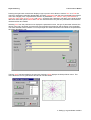
The user has to provide the appropriate information, which consists of a Project ID, a Description and the
project's working directory. Moreover, the user may specify a different set of units (by default Triwaco uses
the time units day and the length unit meter). The definition of all parameters has to be in correspondence
with these units.
Pressing the OK-button the program will create a project file and open the project window. If the user selects
an existing project file he will be prompted whether or not to overwrite this file. An (empty) project window will
be opened and in the menu bar the following two menu options are added: 'data set' and 'Window', each
having their own pull down menu.
4 Setting up a groundwater model-3
Royal Haskoning
Triwaco User's Manual
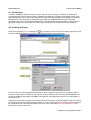
The project window contains an additional, project specific, function key.
Start the default text-editing tool and opens a project description file (project-name.dsc).
The 'data set' pull down menu allows the user to add, open and delete data sets to and from the project
window. These functions, which appear in the upper part of the pull down menu, can also be accessed by the
data set pop-up menu that is activated by the right-hand mouse button.
Data set pull down menu
Info
Open
Delete
Ctrl D
Add
Ctrl A
Dependencies…
Refresh status
Description
Display information on the opened data set
Open an existing data set
Delete the selected data set
Add a new data set to the project
Display data set dependency window
Check and update status indicator
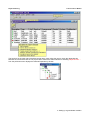
Every data set will be added to the project window of the current modelling project. The project window
displays the following information.
Type
Grid
Based on
Transient
Phreatic
Var. dens.
Description
Subdirectory
Description of type of data set.
Finite Element or Finite Difference grid to be used for calculations
Data set with (hydrogeological) parameters to which this set refers
Indicates whether or not transient calculations are carried out
Indicates whether or not the uppermost aquifer is phreatic
Indicates whether or not the variable density module is used
Descriptive commentary of the data set and its use
Name of the subdirectory for this data set
4 Setting up a groundwater model-4
Royal Haskoning
Triwaco User's Manual
The functions in the lower part of the data set pull down menu allow the user to check the dependencies
between the various data sets of one project and to refresh the status indicators. Selecting 'Dependencies…'
from the pull down menu displays the data set Dependency window.
4 Setting up a groundwater model-5
Royal Haskoning
Triwaco User's Manual
4.3 Creating a Grid data set
4.3.1 Introduction
Triwaco can handle two types of grids, Finite Element Grids and Finite Difference Grids. For the Finite
Element Grid Triwaco uses Triwaco-Flairs for calulating groundwater flow and the grid generator program
Tesnet. For Finite Difference Grid Triwaco uses MODFLOW-96 of the USGS and the grid generator program
Monet. Once the program group (and hence the grid and simulation program) is defined in the ‘Grid
definition’- window, the TriShell processes the initial data, keeps track of changes in data(sets), runs the
corresponding separate modules and carries out different simulation runs.
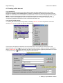
4.3.2 Opening a Grid data set
To create a grid the users opens the grid data set selecting 'data set' 'Add' from the pull down menu and
selecting 'Grid' from the 'create new data set' dialog window.
The program now displays the Grid data set info window and the user supplies the data set name and
directory (if different from the name) and may change the default values for EPFIX and EPPOL. Marking the
section 'Default Grid' with a
the data set's grid will be used whenever the graphical presentation tool Triplot
is started selecting the
function key in the project window's title bar.
4 Setting up a groundwater model-6
Royal Haskoning
Triwaco User's Manual
Choosing the ‘Program group’ allows the user to calculate with the Finite Element Grid (Flairs) by selecting
‘default’ or calculate with the Finite Difference Grid (Modflow) by selecting ‘ModFlow’. When a model is
created using the Variable Density option choose 'Variable Density' (not available in the Standard Package,
see also Chapter 14). The restrictions on using the Finite Difference grid for ModFlow are described in
chapter 5.
The parameters EPFIX and EPPOL define the minimum distances between nodal points of the Finite
Element Grid to be maintained during generation of the grid (valid only for Finite Elements):


EPFIX : Minimal distance between 'Fixed points', e.g. points defined as vertices of the boundary and the
rivers or as sources.
EPPOL : Minimal distance of points within a density polygon, expressed as fraction of the nominal
distance defined for the polygon.
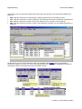
After definition of the grid properties the grid data set is added to the project window. Opening the grid data
set displays the grid data set window, containing the grid parameters: BND, POL, RIV and SRC. In the data
set window's title bar the description file function key appears which allows the user to add comments in a
text file (model.dsc). EPFIX may be defined by polygons to vary EPFIX. EPFIX should be defined by the
parameter name EPFIX.
4.3.3 Defining Grid parameters
The input data for generation of the grid consist of the following items, which are defined by the parameters
from the grid data set:

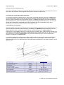
The model area, defined by the grid boundary. The boundary of the model will be defined by the
corner points of a polygon (the parameter BND of the grid data set). The number of nodes to be
generated on each boundary segment can either be specified by the user (by editing the input file)
or be generated by the program using the node distances specified in the density polygon map.

The rivers (line elements), strings of line segments between river points. The input for a river
contains the river points (the parameter RIV of the grid data set). The river segments between the
points are straight. The number of nodes that will be placed on a segment can be specified by the
user (by editing the input file) or calculated by the program using the node distances specified in
the density polygon map. The numbering of the rivers (defined in the corresponding map file) is not
necessarily sequential. The only demand, regarding the numbering of the rivers, is that each river
has a unique ID, defined in the par file. Rivers may be defined by a single line or by a number of
parallel lines. In the latter case some additional editing of the input file is required. Other lineshaped elements (a mountainside or fracture zone) may be incorporated in the grid by defining a
river with an ID equal to 0.

The source points (fixed-point), which can be surrounded by support circles defining small elements.
The location of each source is specified in the input (the parameter SRC of the grid data set). The
source nodes will be marked in the generated grid, but do not necessarily have to act as a source or
sink, they can also be put at the location of monitoring wells, to get more accurate results than by
interpolation between the three nodes of an element. The user can specify extra nodes to be created
around the sources (Only for Finite Element grid, NOT for Finite Difference grid). The extra nodes will
be located at concentric circles around the fixed point. The radii of the circles and the number of
nodes on each circle are specified by the user (Select 'Grid' 'Define support circles' from the menu
bar or by editing the input file). The numbering of the sources (defined in the corresponding map
file) is not necessarily sequential. The only demand, regarding the numbering of the sources, is that
each source has a unique ID. To define a fixed point to be added to the grid but not to be regarded
as a source-node requires some additional editing of the input file.

The size of the elements within areas defined by the node distance of the density polygon map (the
parameter POL of the grid data set).
4 Setting up a groundwater model-7
Royal Haskoning
Triwaco User's Manual
Summarizing, the four grid specific parameters which define the structure of the Finite Element/Difference
Mesh are:




BND : Map file containing one single polygon, defining the boundary of the model's domain
POL : Map file containing a number of polygons, each defining an area with user defined node distances
RIV : Map file containing a number of lines, each defining a river, channel or other waterway.
SRC : Map file containing a number of points, each defining the location of a groundwater abstraction or
infiltration
Double clicking on one of the parameters causes the graphical editor DigEdit (How to use DigEdit is
explained in chapter 8) to open. For each of the grid parameters the user creates a map file containing the
topographical layout of that parameter within the model's domain.
4 Setting up a groundwater model-8
Royal Haskoning
Triwaco User's Manual
Pressing the right hand mouse button displays a pop-up menu which allows to retrieve 'Info' or to 'Edit' the
map file or parameter values file (the par file). Choosing 'Parameter' from the menu bar displays a pull down
menu with a slightly more comprehensive selection of possibilities: 'Info', 'Delete', 'Add' ('User defined' or
'Internal'), 'View' ('Map' or 'Par'), 'Copy' and 'Paste'. Accessing the 'Parameter' pull down menu while the Grid
data set is active the options 'Delete' and 'Add' are omitted because only the four parameters mentioned are
used and all four are needed.
Selecting 'Info' from the pull down menu displays the parameter's name, the type of parameter selected, the
names of the map, parameter and result files used to define the parameter and the status of the parameter.
The status indicator shows whether or not map and par files have been defined and whether the parameters
have been allocated or not.
The item 'Grid' has been added to the menu bar. Selecting 'Grid' displays the Grid pull down menu. This
menu allows the user to generate the Grid and to view the results.
4 Setting up a groundwater model-9
Royal Haskoning
Triwaco User's Manual
Selecting 'Define support circles' from the pull down menu allows the user to add one or more Support
circles to the sources nodes. The user can choose from a number of predefined radii and sets the number of
nodes to be generated on the support circles by selecting the appropriate items from the dialog window.
The Support circles allow the user to define a locally very dense grid, which improves the results of the
calculation of groundwater flow in the vicinity of abstraction or infiltration wells. Because of the nature of the
finite difference grid this option is available for finite elements only.
4.3.4 Generating the Grid
Once a map file is created for all grid parameters, the grid can be generated. Select 'Generate Input file' from
the pull down menu to create the grid.tei input file needed for the grid generator. The input file may be
viewed selecting 'View' 'Input', which opens the input file using the default text editor. See paragraph 4.3.6 for
the input data description of the grid.tei.
To start the grid generator one should select 'Start grid generation' from the pull down menu. TriShell starts
the grid generator in a separate window.
Alternatively, the grid generate program may be run stand-alone choosing the corresponding icon from the
Triwaco Program Folder. In that case, however, the program will not be displayed in the Tasks window.
The grid generator writes the results to the standard ASCII text file grid.teo. This file can be viewed (in text
mode) selecting 'View' 'Grid output as text' from the pull down menu. Selecting 'View' 'Print' opens the
execution log file (grid.tep), which contains all information regarding the grid generating process. See
paragraph 4.3.7 for an example output file.
4.3.5 Viewing the Grid
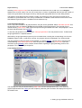
The resulting Grid may be viewed selecting 'View' 'Grid' from the Grid pull down menu. This starts the
graphical presentation tool TriPlot (see also chapter 9) loads the grid information and displays the layout of
the model's area.
4 Setting up a groundwater model-10
Royal Haskoning
Triwaco User's Manual
4.3.6 Input data description
The input file (grid.tei) for generation of a Finite Element grid or Finit Difference grid is a readable ASCII text
file. For the generation of a Finite Element grid the program Tesnet is used. For generating a Finite
Difference grid the program Monet, is used for which, because of the nature of the Finite Difference grid,
restrictions apply (paragraph 5.4.2). In some cases an alternative gridgenerator may be used (paragraph
4.3.8). The grid.tei contains the following contents:
Set 1:
HEAD
Format A40
· identification of project or grid
HEAD is an alphanumerical string for identification of the project's grid
Set 2:
NBP, NRIV, NSRC, NPOL, EPFIX
· number of boundary input points
· number of rivers, line elements
· number of sources, fixed points
· number of density polygons
· absolute minimum distance between fixed and nodal
points
Format Free
NBP, NRIV, NSRC and NPOL are integer values and 0 (the value is obtained from the corresponding
parameter map files BND, RIV, SRC and POL);
EPFIX is a real value 0. EPFIX may be defined by polygons to vary EPFIX. The file should be defined by
the parameter name EPFIX.
Set 3a:
XB1, YB1
· coordinates first boundary point
Format Free
· coordinates next input point
(i = 2, …, NBP)
· code for generation BND nodes
Format Free
XB1, YB1 are real values
Set 3b:
XBi, YBi, IBP
XBi, YBi are real values; the coordinates of the last boundary point (XBNBP, YBNBP) should be equal to those of
the first boundary point (XB1, YB1).
IBP is an integer, either -1 (default) or >0
. If IBP = -1
. If IBP > 0
the number of nodes generated depends on the node density.
the number of nodes generated between boundary point 'i' and boundary point 'i-1' equals IBP.
Set 3b will be repeated (NBP-1) times.
Set 4a:
XR1, YR1, IRIV, Nrivp
· coordinates first river point
· river ID
· total number river input points
Format Free
XR1, YR1 are real values
IRIV is an integer value 0;
. If IRIV=0 the line is not considered a 'river' and is not included in the number of rivers NRIV (Set 1). Lines with IRIV=0 should be
preceded and followed by lines with IRIV 0. More than one line with IRIV=0 may be present in the input file.
Nrivp is an integer value >2
Set 4b:
XRi, YRi, IRIV, IRP, WIDTH
XRi, YRi are real values
IRIV is an integer value
· coordinates nest input point
(i = 2, …, Nrivp)
· river ID
· code for generation river nodes
Format Free
0; the same as for Set 4a.
4 Setting up a groundwater model-11
Royal Haskoning
Triwaco User's Manual
IRP is an integer, either -999, -1 (default) or >0
. If IRP = -999
. If IRP = -1
. If IRP > 0
the number of nodes generated equals the node density.
the number of nodes generated equals half the node density.
the number of nodes generated between river input point 'i' and river input point 'i-1' equals IRP.
WIDTH is an optional real value
0.
. If WIDTH is given TESNET generates an additional line at both sides of the river defined by the coordinates, the distance of the
additional lines to the central line being equal to WIDTH.
Set 4b will be repeated (Nrivp-1) times.
Set 4a and 4b will be repeated (NRIV + NR0) times.
NR0 being the number of times a river has been defined with IRIV=0.
Set 5a:
XS, YS, Ncir, Npc
· coordinates of source point
· nr of support circles
· nr of nodes to be generated on each support circle
Format Free
XS, YS are real values
Ncir is an integer value, either -1, 0 (default) or >0;
. If Ncir = 0
. If Ncir = -1
. If Ncir > 0
there are no support circles and set 5b should be skipped.
there is only one support circle, the radius of the support circle will be read from an additional value R1 on the same
record: XS, YS, Ncir, Npc, R1. Set 5b should be skipped.
Ncir support circles are present, the radii of which are given in set 5b.
Npc is an integer value, either -1, 0 (default) or >0.
. If Npc > 0
. If Npc = -1
Npc points are added to each support circle.
there is no support circle, the point is not considered a 'source' and is not included in the number of sources NSRC
(Set 1). Lines with Npc=-1 should be preceded and followed by sets defining regular sources. More than one point
with Npc=-1 may be present in the input file.
Set 5b:
R1, R2, …, Ri, …, Rncir
Format Free
· radii of support circles
R1, R2, Ri etc are real values
0.
Set 5b should be skipped if Ncir equals -1 or 0.
Set 5a and 5b will be repeated (NSRC + NFP) times.
NFP being the number of times a fixed point has been defined that is not a source; Npc=-1.
Set 6a:
IPOL, Npp, DIST, EPPOL
·
·
·
·
sequential polygon number
nr of polygon input points
node distance for nodes generated within the polygon
minimum distance to previously generated nodes
Format Free
IPOL is an integer value >0
Npp is an integer value >3
DIST and EPPOL are real values >0, by default EPPOL equals half the value of DIST.
Set 6b:
XPi, Ypi
· coordinate of polygon input point
(i = 1, …, Npp)
Format Free
XPi and YPi are real values.
Set 6b will be repeated Npp times. The coordinates of the last input point (XPNpp, YPNpp) should be equal
to the coordinates of the first input point (XP1, YP1).
Set 6a and 6b will be repeated NPOL times (Set 1).
The last polygon, having the largest node-distance, should cover the whole model area. Hence, all corner
points of this polygon should be outside the model's boundary (parameter BND).
4 Setting up a groundwater model-12
Royal Haskoning
Triwaco User's Manual
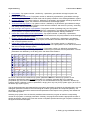
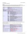
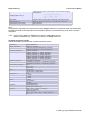
Example of a grid input file grid.tei
SET
Example text
Parameter
Description
1
FE Grid
HEAD
identification of project or grid
2
83335
IBP, ..
NRIV, ..
NSRC, ..
NPOL, ..
EPFIX
number of boundary input points
number of rivers, line elements
number of sources, fixed points
number of density polygons
absolute minimum node distance
3a
3b
3b
3b
3b
3b
3b
3b
147006 410600
146783 409502 –1
147224 408645 –1
148316 407983 –1
150005 408537 –1
149967 410841 25
148472 411106 –1
147006 410600 –1
XB1, YB1
XB2, YB2, IBP
XB3, YB3, IBP
.
.
.
.
XBN, YBN, IBP
coordinates first boundary point
4a
148844 411097 1 24
XR1, YR1, IRIV, Nrivp
coordinates first river point
river ID
total number of river points
4b
148800 410974 1 –1
XR2, YR2, IRIV, IRP
coordinates next river point
river ID
code for generation RIV nodes
4b
4b
4b
4b
4b
4b
4b
4b
4b
4b
4b
4b
4b
4b
4b
4b
4b
4b
4b
4b
4b
4b
148682 410794 1 –1
148550 410653 1 –1
148494 410553 1 –1
148479 410444 1 –1
148488 410373 1 –999
148588 410405 1 -1
148668 410179 1 -1
148582 410014 1 -1
148574 409899 1 -1
148635 409687 1 11
148706 409578 1 -1
148759 409299 1 -1
148862 409025 1 -1
148956 408878 1 -1
149118 408807 1 -1
149250 408716 1 -1
149283 408542 1 -1
149289 408404 1 -1
149274 408263 1 -1
149289 408201 1 -1
149359 408122 1 -1
149445 408022 1 -1
XR3, YR3, IRIV, IRP
.
.
.
.
.
.
.
.
.
.
.
.
.
.
.
.
.
.
.
.
XRN,YRN,IRIV,IRP
(default value for IRP = -1)
IRP < 0; automatic generation
Distance equal to 0.5 node distance
4a
4b
4b
4b
148479 410373 2 15
148285 410373 2 -1
XR1,YR1,IRIV,Nrivp
XR2,YR2,IRIV,IRP
.
XRN,YRN,IRIV,IRP
Repeat set 4 for next river
5a
148351 409687 2 6
XS, YS, Ncir, Npc
5b
10 25
R1, R2
coordinates source point
nr of support circles (default value Ncir = 0)
nr of nodes on support circle (default Npc = 0)
Radii of support circles
nr of radii equals Ncir (set 5a)
Repeat set 5a and 5b for each source point
6a
1 9 10 3.3
IPOL,Npp,DIST,EPPOL
polygon ID
number of points of polygon
node distance
minimum distance factor for polygon
6b
6b
148261 409843
148006 409675
XP1, YP1
XP2, YP2
coordinates first polygon point
coordinates next polygon point
IBP < 0; automatic generation
->distance equal to node distance
IBP > 0; nr of nodes to generate
-> distance = section length / nr intervals
N = IBP (see set 2)
IRP = -999; automatic generation Distance
equal to node distance
IRP < 0; automatic generation
IRP > 0; nr of nodes to generate
N = Nrivp (see set 4a)
4 Setting up a groundwater model-13
Royal Haskoning
Triwaco User's Manual
SET
6b
6b
6b
6b
6b
6b
6b
Example text
148010 409490
148335 409308
148726 409420
148698 409567
148628 409675
148568 409881
148261 409843
Parameter
.
.
.
.
.
.
XPN, YPN
Description
6a
6b
6b
6b
2 10 50 16.5
148469 410459
IPOL,Npp,DIST,EPPOL
XP1, YP1
Repeat set 6 for next polygon
148469 410459
XPN, YPN
6a
3 8 250 82.5
6b
146916 410810
6b
146518 409435
6b
146991 408430
6b
148311 407923
6b
150093 408445
6b
150202 410885
6b
148490 411174
6b
146916 410810
File ends with an empty line
END OF FILE
IPOL,Npp,DIST,EPPOL
XP1, YP1
.
.
.
.
.
.
XPN, YPN
N = Npp (see set 6a)
Repeat set 6 for next polygon
Nr of sets equals NPOL (set 2)
4 Setting up a groundwater model-14
Royal Haskoning
Triwaco User's Manual
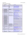
4.3.7 Output data description
The grid generation program creates a formatted sequential file containing all information about the Finite
Element or Finite Difference grid generated. The output file (grid.teo) consists of 8 data records and 13
parameter arrays or adore-sets, the standard Triwaco format.
Note The information for the Finite Difference is also saved in the grid.teo file. Upon execution of the
ModFlow simulation the grid and paramater data is converted to standard ModFlow format. In addition the
grid information is also saved as Finite Element data.
The first record contains the project identification. The next seven records (2 through 8) contain info
concerning the finite element grid. This information consists of literal text followed by an integer number:
Description
Type
NUMBER NODES
NUMBER ELEMENTS
NUMBER FIXED POINTS
NUMBER SOURCES
NUMBER RIVERS
NUMBER RIVER NODES
NUMBER BOUNDARY NODES
NUMBER OF ROWS
NUMBER OF COLUMNS
NUMBER SOURCE CELLS
NUMBER RIVER CELLS
ROTATION ANGLE
NOD
NEL
NFIX
NSRC
NRIV
NRP
NBP
Tesnet,
Trinet
X
X
X
X
X
X
X
Monet
ReGuGrid
X
X
X
X
X
X
X
X
X
X
X
X
X
X
X
X
X
Depending on the type of grid generator used adore sets with the following labels are written to the grid
output file:
1
2
3
4
5
6
7
8
9
10
11
12
13
14
Finite Element
X-COORDINATES NODES
Y-COORDINATES NODES
ELEMENT NODES 1
ELEMENT NODES 2
ELEMENT NODES 3
ELEMENT AREA
NODE INFLUENCE AREA
SOURCE NODES
NUMBER NODES/RIVER
LIST RIVER NODES
LIST BOUNDARY NODES
BOUNDARY SEGMENTS
RIVERNUMBER
SOURCENUMBER
16
17
18
19
20
21
Finite Difference
DELC
DELR
INACTIVE CELLS
SOURCE CELLS
RIVER CELLS
RIVER LENGTH
The parameter names of theadore-sets are self-explanatory. Sets 8 and 14 (SOURCE NODES,
SOURCENUMBER) are omitted if the number of sources equals 0. Sets 9, 10 and 13 (NUMBER
NODES/RIVER, LIST RIVER NODES, and RIVERNUMBER) are omitted if the number of rivers equals 0.
Furthermore, a second output file is generated with the default name grid.tep. This print output file consists
of an echo of the input, some intermediate results, and data of the generated grid. The print output file is
4 Setting up a groundwater model-15
Royal Haskoning
Triwaco User's Manual
useful to track a possible error in the input file. The file contains the number of boundary nodes, river nodes
and source nodes that have been read and generated by the program. Moreover, nodes that are eliminated
or moved because their distance to neighboring points is less than the specified minimum distance (EPFIX)
are listed and the remaining number of boundary, river and source nodes is printed. Once the grid has been
generated, the minimum and maximum element area and the coordinates of the nodes are printed.
4.3.8 Alternative grid generators
Trinet
In addition to the standard grid generation program Tesnet and Monet there are other grid generation
programs included. One of these is Trinet, which is a Finite Element grid generator (TIN). The program is
much faster but has some restrictions. Trinet does not support the generation of support-circles around
sources or the generation of rivers consisting of multiple parallel line elements. It reads the standard grid.teo
input file and generates a standard Triwaco grid output file.
ReGuGrid
In addition to the standard grid generation program Tesnet and Monet there are other grid generation
programs included. One of these is ReGuGrid, which produces a Finite Difference grid. The cells of a grid
generated with ReGuGrid are all equally sized (equal width and height). This grid has the same restrictions as
as grids generated by Monet. Additionally sources, rivers and density polygons are ignored. For the definition
of the cell size ReGugrid uses the smallest value from the density polygons (if more than one is defined).
4 Setting up a groundwater model-16
Royal Haskoning
Triwaco User's Manual
4.4 Creating an Initial data set
4.4.1 Introduction
In the initial data set the user defines the conceptual model. All original data is stored grid independently, so it
is possible to make a model with different (type of) grids but with the same initial data.
4.4.2 Opening an Initial data set
Selecting 'data set' 'Add' from the pull down menu and 'Initial' from the 'create new data set' dialog window
the 'initial data info window' is displayed and the user has to provide information regarding the
hydrogeological system. The 'initial data info window' is divided in two parts. In the upper part a description,
the directory name and the path have to be given. In the lower part of the window the properties defining the
hydrogeological system are recorded.
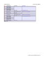
4.4.3 Defining model properties
The properties defining the hydrogeological system are recorded in the 'Main settings' area, the lower part of
the 'initial data info window'. Subsequently the following information has to be provided by checking the tick
box ( ) or leaving it blank (
).
Description
Unchecked box (
)
Checked box (
)
All aquifers are confined
Phreatic upper aquifer
No Variable Density is used
Variable Density is used
Steady state calculations
Transient calculations
No modeling of vertical groundwater flow
Modeling of vertical groundwater flow in
Unsaturated zone modeling
in the unsaturated zone (FLUZO)
the unsaturated zone.
* When a model is created for using the Variable Density additional parameters have to be defined (see also chapter 14).
Phreatic conditions
Variable Density*
Transient
At the right hand side of the 'Main settings'
area the number of aquifers can be
selected in the corresponding box and the
type of topsystem, representing the upper
boundary condition, can be selected.
Topsystems
The discharge or recharge of groundwater at the top of the first aquifer can be characterized by the so-called
top-systems. A top-system describes the interaction between the groundwater system and a
drainage/infiltration system consisting of generally small surface waters and drains. A short description of the
topsystems is listed below. A more detailed description is given in Appendix A.
4 Setting up a groundwater model-17
Royal Haskoning
Triwaco User's Manual
1. Precipitation; Top-system number 1, defined by 1 parameter; groundwater recharge is equal to the
precipitation excess.
2. Polder with fixed water level; Top-system number 2, defined by 3 parameters; groundwater recharge
and discharge depend on a fixed water level and the (total) resistance of the drainage/infiltration system.
3. Phreatic drainage; Top-system number 3, defined by 3 parameters; groundwater discharge depends on
the head in the top aquifer, the resistance and the base of the drainage system.
4. Three-level drainage system; Top-system number 4, defined by 13 parameters; groundwater recharge
5.
6.
7.
8.
9.
or discharge depends on the precipitation excess and the resistance and levels of a primary, secondary
and tertiary drainage/infiltration system.
Pipe drainage and irrigation or precipitation; Top-system number 5 (drainage only) and Top-system
number 6 (both drainage and infiltration), defined by 8 parameters; groundwater discharge depends on
the precipitation or irrigation excess, the head in the top aquifer and the drainage resistance.
Polder with a fixed water level and precipitation; Top-system number 7, defined by 4 parameters;
groundwater recharge or discharge depends on a fixed water level, the (total) resistance of the drainage
system and the precipitation excess.
Phreatic drainage with precipitation; Top-system number 10, defined by 4 parameters; groundwater
discharge depends on the head in the top aquifer, the resistance and the base of the drainage system
and on the precipitation excess.
Polder with a fixed water level and single drainage system; Top-system number 11, defined by 5
parameters; groundwater recharge or discharge depends on the precipitation excess and the resistance
and level of a single drainage system.
Predefined recharge or discharge characteristic; Top-system number 12, defined by 5 parameters;
groundwater recharge or discharge depends on meteorological quantities and soil parameters. The soil
parameters are obtained by curve fitting of the Van Genuchten relations.
IR
1
2
3
4
5
6
7
8
9
10
11
12
RP1 RP2
P
HP
C0
HS
W
P
C0
P
HS
P
HS
P
C0
not in use
not in use
P
W
P
C0
P
ETmx
RP3
RP4
RP5
RP6
RP7
RP8
RP9
RP10
RP11
RP12
RP13
W
BD
HP
Hd
Hd
W
W d,1
HT
HT
HP
W d,2
Kv
Kv
W d,3
Kh
Kh
W i,1
L
L
W i,2
R
R
W i,3
BD1
BD2
BD3
HS
BD
Wd
a
HS
Wi
b
Hp
HS
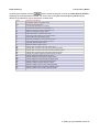
As can be noticed from this table the top system parameters RPxx for different top systems do not
necessarily represent the same physical parameter. For example, parameter RP1 may represent
precipitation (P), the surface level elevation (Hs) or the controlled water level (Hp). Moreover, different top
systems require a different number of parameters, ranging from only one (for top system type 1) to as much
as thirteen (top system type 4).
The physical parameters associated with the top system parameters are listed in the following table. One can
distinguish parameters related to the meteorological condition (precipitation and evapotranspiration), soil
parameters, surface and surface water levels and parameters with respect to the geometry and resistances
of the drainage system.
Selecting a top system from the list with predefined sets causes the program to load the corresponding
number of top system or recharge parameters. Similarly, the program also loads the appropriate number of
aquifer parameters, taking into account the number of aquifers specified and the type of aquifer condition for
the upper and lowermost aquifer.
4 Setting up a groundwater model-18
Royal Haskoning
Triwaco User's Manual
Confirming the selection with the
-button causes the program to open the 'Initial data set window',
displaying all model parameters needed. For each of the model parameters a map and par file may be
defined or the parameter may be assigned a constant value.
Name
P
ETmx
A
B
C0
Hd
HP
HS
HT
Kh
Kv
L
R
BD
BD1
BD2
BD3
W
Wd
W d,1
W d,2
W d,3
WI
W i,1
W i,2
W i,3
Definition of parameter
Precipitation excess or irrigation excess
Maximum Evapotranspiration
soil parameter obtained by curve fitting
soil parameter obtained by curve fitting (b > 1)
Hydraulic resistance of semi-pervious top layer
Drain level of system of (pipe)—drains
Polder water level or controlled water level
Surface level (with respect to the ordnance level)
Level of base of semi-pervious top layer
Horizontal permeability of semi-pervious top layer
Vertical permeability of semi-pervious top layer
Horizontal distance between drains
Wetted perimeter of (pipe)—drains
Drainage base or bottom level of the (open) drains
Drainage base or bottom level of the primary drainage system
Drainage base or bottom level of the secondary drainage system
Drainage base or bottom level of the tertiary drainage system
Drainage or infiltration resistance between ditches or drains
Drainage resistance between ditches or drains
Drainage resistance of the primary drainage system
Drainage resistance of the secondary drainage system
Drainage resistance of the tertiary drainage system
Infiltration resistance between ditches or drains
Infiltration resistance of the primary drainage system
Infiltration resistance of the secondary drainage system
Infiltration resistance of the tertiary drainage system
4 Setting up a groundwater model-19
Royal Haskoning
Triwaco User's Manual
4.4.4 Defining model parameters (general)
To define a model parameter the user has to provide a map and par file and has to specify the allocator
(appenix C) to be used. The allocator defines how parameter values are assigned to the nodes of the grid.
Triwaco opens the 'Initial data set window' with a set of default allocators, depending on the type of
parameter. An overview of parameter types is listed here (see appendix B for a complete overview and the
lay out of the map, parameter and corresponding ado files).
Double clicking on one of the parameters starts the graphical editor DigEdit (Chapter 8). If map and par files
exist for the parameter considered these files are loaded, if not the screen remains empty. For each of the
parameters the user creates a map file. This file contains the topographical layout of the parameter
concerned, consisting of a set of points, lines or polygons that are (partly) within the model's domain. Each
graphical object in the map file will be assigned a value; these parameter values are stored in the par file,
containing the object's ID and the parameter value.
Pressing the right hand mouse button displays a pop-up menu which allows to retrieve 'Info' or to 'Edit' the
map or par file. Choosing the 'Parameter' pull down menu from the menu bar displays a slightly more
comprehensive selection of possibilities: 'Info', 'Delete', 'Add' ('User defined' or 'Internal'), 'View' ('Map' or
'Par'), 'Copy' and 'Paste'.
4 Setting up a groundwater model-20
Royal Haskoning
Triwaco User's Manual
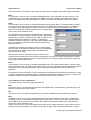
Selecting 'Info' from the pull down menu displays the 'parameter info window ', with the parameter's name,
the type of parameter selected, the names of the map and par files used to define the parameter and the
status of the parameter. The status indicator shows whether or not the map and par files have been defined
and whether the parameter has been allocated or not. The 'Settings area' of the 'parameter info window '
allows the user to change the parameter type, the allocator and the default value. Moreover it allows the
definition of an expression, which relates the selected parameter to other model parameters.
The name in the General information area is the predefined parameter name that is recognized by Triwaco.
The description may be modified; this is a short descriptive comment characterizing the parameter. The
names of the parameter, map and result file are generally the same as the parameter name and differ only by
their extension.
4 Setting up a groundwater model-21
Royal Haskoning
Triwaco User's Manual
In the Settings area the proper allocator type has to be provided and the default value for the parameter
considered has to be given. This deafualt value will be assigned to the parameter if the allocator type is set to
"Const" or for parts of the model's domain that are not covered by the parameter's map file.
Triwaco includes a range of powerful geo-processors for 1D to 4D interpolation. The processors are called
allocators since they are used to assign (allocate) parameter GIS maps/values to the individual nodes or cells
of the grid. Most allocators can be used for different types of parameters. For source, river and boundary
parameters specific allocators are available. Other allocators are used for distributed parameters only
(assigning a parameter value to each node of the grid). In appendix C descriptions and usage of all allocators
can be found.
Optionally the parameter may be related to other parameters by a (mathematical) expression. The allocator
type has to be set to "Expression" and the expression itself should be entered in the Expression-box (see
appendix C for all options using the expression allocator).
After having provided all information needed, including the necessary map and par files, the status indicator
of the parameter changes from
to .
4.4.5 Definition of boundary conditions
The type of boundary condition is defined by the parameter IBi. Multiple type boundary conditions may be
defined for different parts of the model boundary. For those parts of the model boundary for which IBi=0 a
constant head boundary applies (default). A constant head boundary implies the definition of the boundary
head by the parameter BHi, which defines the constant head in aquifer i.
For IBi=1 a constant flux boundary applies. Consequently the constant flux has to be defined by the
parameter BBi, which defines a constant flux (m3/d per m) in aquifer i, and/or the parameter BAi, which
defines the the slope of the boundary flux (m3/d per m2) in aquifer i. The flux is defined as Q=BA * PHI + BB,
where PHI is the groundwater head on the boundary.
Boundary type parameters are defined by so called `Linked Points` in DigEdit (chapter 8). A linked point is
used to assign values to grid parameters: boundary and rivers(line elements). These points, when used to
define boundary conditions, by definition are linked to ID 1, which represents the ID of the boundary. Each
point is given a value for flux or head depending on the condition defined. These parameters are allocated
with the allocator ParBou. This allocator will interpolate (lineair) between the points.
4.4.6 Definition of river (line-element) parameters
The river activity is controlled by the parameter RAi.
RA=0
4 Setting up a groundwater model-22
Royal Haskoning
Triwaco User's Manual
The line elements for which RAi=0 are inactive and are treated as regular nodes/cells during the simulation.
RA=1
A line element or river for which a constant head applies RAi=1. The properties of the line element or river
are defined by four parameters; HRi defines the waterlevel or head in aquifer i, RWi defines the width in
aquifer i, CDi defines the drainage resistance in aquifer i, CIi defines the infiltration resistance in aquifer i.
RA=2
A line element or river for which a constant discharge/recharge applies Rai=2. A HOrizontal BOring (HOBO)
or a range of small wells can be schematised as a single or multiple line-element in aquifer i. A HOBO is a
line element (river) representing the wells in a section. For each line element an abstraction rate can be
defined. The model will calculate the water level for that particular
section at the given abstraction rate.
The properties of the line-element are defined by five parameters;
HRi defines the initial waterlevel or head in aquifer i , RQi defines
the discharge in aquifer i, RWi defines the width in aquifer i, CDi
defines the drainage resistance in aquifer i, CIi defines the
infiltration resistance in aquifer i. HR is the initial waterlevel defined
by the user and should be close to the expected waterlevel for
iteration purposes.
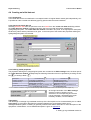
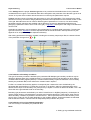
In addition line-elements can also be clustered. The discharge,
defined by RQ, of individual line-elements are evenly distributed in
such a way that the head (or waterlevel) of all clustered lineelements will be the same.
The line-elements to be clustered are linked to the main lineelement by the parameter RCi, which contains linked points. For each line-element a linked point is used to
link it to the main line-element, as shown in the screenshot. In this case line-element with ID 637 is linked to
the main line-element with ID 1587.
RA=3
A line element or river for which a constant head applies RAi=3. This option equal to RAi=1 until PHI1 drops
below the bottom of the river (BRi). In that case the flux is no longer governed by (HR-PHI)/CI but is limited to
a maximum flux governed by (HR-BR)/CI. Which corresponds to way the fluxes are governed by the
topsystem.
The properties of the line element or river are defined by five parameters; HRi defines the waterlevel or head
in aquifer i, RWi defines the width in aquifer i, CDi defines the drainage resistance in aquifer i, CIi defines the
infiltration resistance in aquifer i, BRi defines the bottom level of the river in aquifer i.
4.4.7 Definition of source parameters
The source activity is controlled by the parameter ISi.
IS=0
Sources for which a constant abstraction/injection rate applies ISi=0. The abstraction(-) and injection(+) are
defined by the parameter SQi in aquifer i.
IS=1
Sources for which a constant head applies ISi=1. The head is defined by the parameter SHi in aquifer i.
IS=2
In addition sources with a constant abstraction/injection rate may be clustered. This option is usefull when
modelling a section of wells with one discharge point (suction pipe). Then for this point the abstraction rate
can be defined (in fact the sum of all is taken). The model will calculate the water level for that particular
section at the given abstraction rate.
Another case may be a source with multiple well screens each in a different aquifer. Then for this source the
abstraction rate can be defined. The model will calculate the water level, which will be the same in all well
4 Setting up a groundwater model-23
Royal Haskoning
Triwaco User's Manual
screens, at the given abstraction rate.
Sources are clustered by defining the parameter SNi. Sources for which SN=0 are not clustered. Sources for
which SN=n are clustered. So when SN=22 these sources are part of cluster 22, etc.
4.4.8 Definition of hydrogeological parameters
For confined conditions the transmissivity in each aquifer is generally defined by TXi (m2/d). Triwaco does
recognize permeability (PXi) provided top and base of the aquifer, respectively RLi and THi , is defined as
well. For phreatic conditions in the upper aquifer (aquifer 1) Triwaco calculates the transmissivity based on
the permeability (PX1), base of the aquifer (TH1) and the calculated grondwatertable (PHIT). The top of the
aquifer (RL1) needs also to be defined to account for situations wth groundwatertables rising above
groundlevel. The resistance of each aquitard is defined by CLi (d).
4.4.9 Definition of anisotropy
Although Triwaco assumes that transmissivities and permeabilities of all aquifers are by default isotropic, the
user can define an anisotropic transmissivity (or permeability). For ModFlow the transmissivity tensor can
only be defined in the Kx, Ky and Kz direction co-linear to the grid. Whereas for Triwaco-Flairs the
transmissivity (or permeability) tensor may vary through the model area, which implies that the principal axes
of the tensor can have different orientations in different points of the model domain (Kxx, Kxy, Kyx, Kyy, Kzz). So
when anisotropy is important Triwaco-Flairs is the prefered simulation program. The input description
therefore concentrates on Triwaco-Flairs.
For confined conditions the transmissivity in each aquifer is defined in the direction of the principal axis by
TXi and TYi. Triwaco does recognize permeability (PXi and PYi ) provided top and base of the aquifer,
respectively RLi and THi , is defined as well. The angel between the direction of TX and the positive X-axis is
defined by ALi.
Parameter type
Type of Boundary condition
Type of Source Input
River Activity
Type of Top system
Boundary Condition parameter
Source parameters
River parameters
Distributed parameters
Preferred allocator
ParBou
SrcParAdo
ParRiv
Const
ParBou
SrcParAdo
ParRiv
Various available
Parameter name
IBi
ISi
RAi
IR
BHi, BAi, BBi
SQi, SHi, SNi
HRi, RWi, CDi, CIi, RQi
RPxx, CLi, TXi, PXi, etc.
4 Setting up a groundwater model-24
Royal Haskoning
Triwaco User's Manual
4.4.10 Definition of expressions
General
The Expression allocator evaluates an expression and calculates (creates) a new Adore-block. An
expression may contain set-names, numbers, functions, factors and operators. Three types of operators may
be distinguished: mathematical operators, relational operators and logical operators.
Definition
Set-names
Numbers
Factors
Mathematical operators
Relational operators
Logical operators
Functions
Description
Parameter names as defined in Triwaco , consisting of a combination of
alphanumeric characters.
The parameter may be preceded by the name of one of the project’s data sets and a
$-sign: e.g., cal$TX1
integer and real numbers: e.g., 15, -0.456
Consist of numbers, expressions, functions or identifiers.
+, -, * and /
>,
(>=), = (==),
(<=) and <
‘AND’ ('&&'), ‘OR’ ('||') and ‘NOT’ ('=!') and 'IF' 'THEN' ('?') and 'ELSE' (':')
(simple) mathematical functions:
abs(x)
Returns the absolute value of 'x'
atan(y,x)
Returns the arc tangent of ('y/x')
BND(x)
Returns the value of 'x' at boundary nodes
cos(x)
Returns the cosine of 'x'
deg(x)
Converts radians ('x') to degrees
exp(x)
Returns the value of e raised to the power 'x'
Evaluates the logical expression:
IF ('x') THEN ('y') ELSE ('z')
IF(x,y,z)
Equivalent to the expression:
('x')?('y'):('z')
ln(x)
Returns the natural logarithm of 'x'
log(x)
Returns the 10 log of 'x'
max(x,y)
Returns the largest value of 'x' and 'y'
min(x,y)
Returns the smallest value of 'x' and 'y'
Returns the value of 'x' at all Nodes; if the value of 'x' does not
NODE(x)
exist at a Node a zero value (0) is assumed
rad(x)
Converts degrees ('x') to radians
RIV(x)
Returns the value of 'x' at river nodes
sign(x)
Returns the sign of 'x' (-1, 0 or +1)
sin(x)
Returns the sine of 'x'
sqr(x)
Returns the square of 'x'
sqrt(x)
Returns the square root of 'x'
SRC(x)
Returns the value of 'x' at source nodes
tan(x)
Returns the tangent of 'x'
Important note: The setname or data set name should NOT contain an underscore (data_set$set_name).
Examples of expressions
In the following table examples of the more or less frequently used expressions are listed.
PHIT
Result$PHI1
12
PHI1-PHIT
QRCH>0
(PHI1-PHIT) * (QRCH>0 && QKW1>0)
(RL1>TH1)?RL1:(TH1 + 0.01)
IF(RL1>TH1,RL1,TH1+0.01)
adore block with values equal to those of the set with the matching
set name: 'PHIT'
adore block with values equal to those of set 'PHI1' belonging to the
data set with the name: ‘result’
adore block with the constant value 12
adore block with values equal to (PHI1 - PHIT), being the difference
of the adore blocks with set names ‘PHI1’ and ‘PHIT’ respectively
Boolean adore block containing integer values:
equal to 1 where QRCH > 0 and
equal to 0 where QRCH <= 0
Real adore block containing values equal
to 0 where QRCH <= 0 or QKW1 <= 0 and
to (PHI1-PHIT) where both QRCH > 0 and QKW1 > 0
Real adore block containing values equal
to RL1 where RL1 > TH1 and
to (TH1+0.01) where RL1 <= TH1
Real adore block containing values equal
to RL1 where RL1 > TH1 and
to (TH1+0.01) where RL1 <= TH1
4 Setting up a groundwater model-25
Royal Haskoning
Triwaco User's Manual
adore block that contains values equal to the results after evaluating
the expression:
sqrt(log(cos(TX1*TH1)+1)
QRI1/AREA
MIN(PHIT,RP13)
PHIT > RP13 ? RP13 : PHIT
IF(PHIT>RP13, RP13, PHIT)
Specific river flux in m/d (river flux divided by node influence area)
Minimum value of PHIT and RP13: cut off PHIT at surface level
Same as above
Same as above
Note:
Using Boolean expressions the result set will contain integer values if the expression starts with the Boolean
expression and will contain real values if the Boolean expression is preceded with a (real) value or another
expression.
Thus:
(PHI1-PHIT) * (QRCH>0 && QKW1>0) results in a real Adore set and
(QRCH>0 && QKW1>0) * (PHI1-PHIT) results in an integer Adore set.
Complete expression syntax
The following table summarizes the complete expression syntax.
expression =
logical_expression =
relational_expression =
additive_expression =
multiplicative_expression =
term =
typed_factor =
factor =
identifier =
function =
logical_expression
relational_expression
relational_expression '&&' relational_expression
relational_expression '||' relational_expression
additive_expression
additive_expression '<' additive_expression
additive_expression '>' additive_expression
additive_expression '<=' additive_expression
additive_expression '>=' additive_expression
additive_expression '==' additive_expression
additive_expression '=!' additive_expression
multiplicative_expression
multiplicative_expression '+' multiplicative_expression
multiplicative_expression '-' multiplicative_expression
term
term '*' term
term '/' term
typed_factor
typed_factor '^' typed_factor
[typed_factor '^' typed_factor]...
factor
‘-' factor
+' factor
'!' factor
number
'('expression')'
identifier
function(expression)
alphanumeric string
quoted alphanumeric string
abs(..), min(..,..), max(..,..) and sign(..)
log(..), ln(..) and exp(..)
sqr(..) and sqrt(..)
sin(..), cos(..), tan(..), atan(..,..), deg(..) and rad(..)
IF(..,..,..)
4 Setting up a groundwater model-26