Download Ure-etal-IJPVP-2014-Integrated-structural-analysis-tool-part

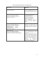
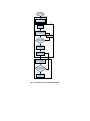
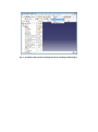
Integrated Structural Analysis Tool using the Linear Matching
Method part 1 – Software Development
James Urea, Haofeng Chena,, David Tippingb
a
Dept of Mechanical and Aerospace Engineering, University of Strathclyde, 75 Montrose
Street, Glasgow G1 1XJ, Scotland, United Kingdom
b
Central Engineering Support, EDF Energy Nuclear Generation Ltd., Barnwood, Gloucester
GL4 3RS, United Kingdom
Abstract
A number of direct methods based upon the Linear Matching Method (LMM) framework
have been developed to address structural integrity issues for components subjected to
cyclic thermal and mechanical load conditions. This paper presents a new integrated
structural analysis tool using the LMM framework for the assessment of load carrying
capacity, shakedown limit, ratchet limit and steady state cyclic response of structures. First,
the development of the LMM for the evaluation of design limits in plasticity is introduced.
Second, preliminary considerations for the development of the LMM into a tool which can
be used on a regular basis by engineers are discussed. After the re-structuring of the LMM
subroutines for multiple central processing unit (CPU) solution, the LMM software tool for
the assessment of design limits in plasticity is implemented by developing an Abaqus CAE
plug-in with graphical user interfaces. Further demonstration of this new LMM analysis tool
including practical application and verification is presented in an accompanying paper.
Keywords: Linear Matching Method (LMM), Structural Integrity, Load Carrying Capacity,
Shakedown limit, Ratchet limit, Steady State Cycle

Corresponding author. Tel.: +44 1415482036
E-mail address: [email protected]
1
1. Introduction
Many Engineering components and structures in defence, aerospace, petrochemical,
automobile and power industries operate under cyclic thermal and mechanical load
conditions, and would include such diverse products as advanced internal combustion (IC)
engine and gas turbine components, high altitude ramjet and rocket motors, chemical
reactor vessels in plastics manufacture, prototype fusion reactors, power boilers, etc. In all
of these applications, it is important to ensure the equipment can operate safely for the
specified design life under the arduous environmental conditions. This requires engineers to
identify possible failure mechanisms and guard against these during the design process [1].
Engineering structures subjected to cyclic loading histories will experience either
elastic/plastic shakedown or ratchetting depending upon the applied load level. Limiting the
behaviour of the structure or component to the elastic range is not an effective approach to
a problem, as this leads to over-conservative design. In many applications, it is acceptable to
allow limited plastic deformation to occur provided it can be shown that the structure
shakes down to elastic action in the first few cycles of load. If the applied load is below the
elastic shakedown limit, ratchetting and plastic shakedown will not occur under repeated
loading. However in some situations, for example in nuclear power applications with cyclic
thermal loading, this elastic shakedown limit can also be over-conservative. Thus an
alternative approach is required to allow plastic shakedown to occur but preclude
ratchetting. In ratchetting, a net increment of plastic strain occurs with each cycle of load
and leads to an incremental plastic collapse over a number of cycles. Guarding against
incremental plastic collapse by the determination of plastic shakedown limit or ratchet limit
is crucial in any design involving cyclic thermal and mechanical loads. Under plastic
shakedown condition, a low cycle fatigue (LCF) analysis would also be undertaken to ensure
the structure does not fail by low cycle fatigue associated with local alternating plasticity,
where the number of cycles to failure is determined by the maximum plastic strain range. A
steady state cyclic analysis is often sought to evaluate the LCF life and address whether
shakedown or ratchetting occurs under the defined cyclic load condition.
Design limits in plasticity for components subjected to cyclic thermal and mechanical load
conditions, including both shakedown and ratchet limits, have attracted the attention of
many researchers. The incremental finite element (FE) analysis [2] allows the investigation
of any type of load cycle but inevitably requires significant computer effort for complex 3D
structures. There has been a recent trend towards the development of direct methods that
2
combine the convenience and efficiency of rule based methods [1] and the accuracy of
incremental FE simulation techniques. Of these simplified direct methods [3-9], the Linear
Matching Method (LMM) [10-14] has become one of the most powerful numerical methods
for generating approximate inelastic solutions and answering specific design related issues
using standard finite element codes. The basis of the LMM is through an idea of representing
histories of stress and inelastic strain as the solution of a linear problem, where the linear
moduli are allowed to vary both spatially and in time. The LMM has been formulated and
implemented for the evaluation of shakedown limit [10, 11] and ratchet limit [12-13]. And
more recently, a new LMM framework was developed to evaluate the steady state cyclic
behaviour of component for the LCF assessment purpose [14].
The LMM is distinguished from the other upper bound or lower bound direct methods by
ensuring that both the equilibrium and compatibility conditions are satisfied to produce
exact solution at each stage of calculations [13], and is counted to be one of the methods
most amenable to practical engineering applications involving complicated thermomechanical load history [15]. However, as many other direct methods, the LMM was initially
implemented into commercial FE software Abaqus [2] using user subroutines developed by
FORTRAN programming language, which is difficult for non-experts to operate. Another
drawback of this implementation is the level of programming experience required to create
and submit an analysis: the alterations to the subroutines required to run each analysis
present issues for everyday use by engineers generally not familiar with FORTRAN. To
remedy this situation and enable widespread adoption of the LMMs in industry, an
integrated software tool is required to not only removes the requirement for manual
subroutine alterations, but also provide additional functionality for subsequent life
assessment calculations.
The main objective of this paper is to develop a new integrated structural analysis tool using
the LMM framework for the assessment of design limits in plasticity, including the
evaluation of limit load, shakedown limit, ratchet limit and steady state cyclic behaviour of
the structure. It will deliver the LMM in a form where it can be readily used by engineers
with the responsibility for design and life assessment decisions on a regular basis. The
software tool would allow engineers to access the LMM solution methods without having to
make any of the changes to the subroutines required to run a LMM analysis as was
previously required.
3
The paper is organized as follows. In Section 2, preliminary considerations are discussed by
examining previous LMM versions and the way of customising Abaqus. In Section 3, a restructuring of the LMM user-subroutines for multiple CPU solution is proposed. The creation
of a Graphical User Interface (GUI) via an Abaqus Plug-in is presented in Section 4. Section 5
briefly discusses the installation and testing of the LMM software tool for the assessment of
design limits in plasticity. Section 6 concludes this paper.
2. Preliminary Considerations
2.1 Previous LMM Versions
The original incarnation of the LMM code was created as Abaqus user subroutines and has
been mainly used for research purposes. A typical LMM analysis consists of two stages [1213]. In the first stage an elastic analysis for each applied load and temperature distribution is
performed using the elastic analysis UMAT subroutine. For each of these analyses the elastic
stress tensor for each integration point is written to a text file, and the integration point
temperature is written to a separate text file. The second stage of this analysis uses a second
UMAT subroutine and these text files to perform the shakedown or ratchet limit calculation.
In this second stage some changes are required to the UMAT code in order to set up the
analysis. For example, the number of integration points per element and the total number of
elements in the model needed to be changed so that the arrays could be sized appropriately.
The code defining the load cycle also requires updating, which reads the stress and
temperature text files to generate the applied stresses at each point in the load cycle.
For an analysis using this set of subroutines both the elastic analyses and the further
shakedown or ratchet calculation are submitted using the Abaqus batch command i.e. the
Abaqus input file for the model is required. This input file is generated using Abaqus CAE for
a complete model. The majority of the content of the input file is common between the
elastic and shakedown calculations (such as geometry and boundary conditions). However
there are some differences which must be performed manually (such as requesting the
energy outputs associated with a UMAT subroutine). A further upgrade of these subroutines
was carried out [16] so that the LMM could be used with minimal code changes, where the
load cycle is defined via a formatted text file which was read by the subroutines. This
significantly reduces the code changes required for an analysis. However, the changes to the
Abaqus input file still needed to be performed manually.
The creation of a formatted text file to configure the LMM analysis was a major step in the
usability of the LMM, and in fact draws a parallel with the way in which any conventional
4
Abaqus analysis operates. In an Abaqus analysis, a FE model needs to be created in Abaqus
CAE and submitted for analysis, although other pre and post processors are often used.
Abaqus CAE then creates a formatted text file (Abaqus input file) which is passed to the
Abaqus solver for solution. The text file for the LMM analysis is equivalent to the input file,
the only difference being that it is created manually. The creation of a text file is also
adopted here as it is a simple and robust method for passing information from the LMM
user interface into the subroutines. The major aim of this software tool is that the text file is
generated by the user interface rather than manually.
2.2 Customising Abaqus
Abaqus [2] contains a large number of options for the user to customise a model or analysis
for their particular situation. To obtain user-generated solution options the user-subroutines
can be used, which is how the LMM has been implemented. In addition to this Abaqus CAE
contains the option to use scripts to perform operations on the model or results databases.
These scripts are written in the Python open source scripting language [2], and Abaqus has
extended this language to allow operations to be performed within CAE itself. These scripts
can be used to perform all operations which are available through the CAE interface (i.e.
applying loads, meshing, plotting results etc.) and can also query the model or Abaqus
output file (odb) for values. A typical example where scripts serve a useful function is in a
sensitivity analysis, where an automatic process can vary a particular value in a model, resubmit for solution, query the results and decide whether a further iteration is required.
The use of python scripting within Abaqus is a very powerful tool, because options also exist
to use this language to customise the CAE user interface itself. This can be achieved by
creating either an entirely custom CAE interface or a plug-in to the standard CAE. The ability
to create a custom GUI is a powerful tool as the modules and toolsets which are not desired
can be removed and custom functions can be added. Abaqus Viewer is an example of this,
where all the analysis toolsets and modules have been removed, leaving only the
visualisation module for viewing output databases. Plug-ins form another useful avenue of
adding functionality to the Abaqus CAE interface. Plug-ins can be created for a variety of
purposes; commonly they are used to streamline tasks which are complex to perform or are
performed regularly. For the LMM application a plug-in has been selected over a custom CAE
interface. A plug-in can be accessed through the conventional CAE interface during normal
use, whereas a custom CAE would need to be opened separately. An engineer with an
5
existing Abaqus model will be able to access the LMM through CAE, and the plug in will
guide them through the process of entering the information needed to run a LMM analysis.
The creation of a plug-in to gather the required data and format the model will require a set
of subroutines which are compatible with this model configuration and the text file used to
pass in the data for the analysis. The re-structuring of the subroutines to accommodate this
presents an opportunity to re-write them for multiple CPU solution, especially since even
basic desktop computers now have dual or quad core as standard. Some features of the
UMAT code written by Chen [12-14] and Tipping [16] are not amenable to solution with
multiple CPUs.
With all of these considerations, a plug-in has been created and the LMM subroutines have
been re-written. The plug-in posts dialog boxes to gather the required information and data
from the user. When the process is complete, the plug-in configures the model for the LMM
analysis using scripts. The plug-in also writes the text file containing relevant data for the
subroutines. The subroutines themselves have been re-written to allow multiple CPU
solution in the UMAT routine.
The structure and function of the plug-in is dictated by many of the features of the
subroutines and their re-structuring for multiple CPU solution. Therefore the subroutines
will be described in the next section, followed by a description of the plug-in created to use
them.
3. Re-structuring of the Subroutines
Figure 1 shows the general structure of a LMM solution with the new set of subroutines for
various plastic analyses. The starting point of this process assumes that the plug-in has
created a formatted text file containing information about the analysis such as the
convergence tolerance, analysis type, load cycle and temperature dependent material data.
This LMM text file produced by the plug-in will then be read by the subroutine at the
beginning of the analysis. This means that the UMAT subroutine is called for each integration
point which has been defined as a User-material from within Abaqus CAE. Defining areas of
the model as a User-material within Abaqus CAE tells the solver to look to the UMAT
subroutine for the material behaviour of those areas. This solution stage of the analysis uses
the number of CPUs requested by the user, and so this UMAT subroutine must be coded to
accommodate this.
6
As part of the restructuring, all the elastic calculations for the applied loads and the LMM
calculation itself have been incorporated into a single Abaqus analysis. Each elastic
calculation is carried out as a single analysis step within this Abaqus analysis, with the LMM
calculation being performed in the final analysis step. This consolidation into a single Abaqus
analysis means that the passing of stresses and temperatures in text files is no longer
required. Instead the results file itself can be used for storage and access of this information.
When defining a User-material in Abaqus CAE, the user is able to specify the number of
Solution-Dependent State Variables (SDV) for that material. This is the number of memory
spaces available to the UMAT in the output database file, and so is commonly used to
provide contour plots of user defined variable fields calculated during the UMAT solution.
However, the direct access of SDVs within UMAT means that they can also be used as a way
of storing values and data to be used during the analysis. Hence this has been used to pass
elastic stresses and temperatures between the elastic analyses and the LMM analysis,
removing the need for text files and therefore removing this restriction to multiple CPU
solution.
Returning to Figure 1, the UMAT subroutine is divided into elastic and LMM sections. An
elastic analysis is performed for each applied load and the stresses and temperatures are
stored in the SDV slots. When all applied loads have been considered, an intermediate "null"
step is included. This allows key variables in the subroutine to return to zero before
commencing the LMM solution. The LMM solution itself uses the stresses and temperatures
from the SDVs along with the load cycle and material property data read in the
UEXTERNALDB subroutine to perform the calculations.
Within the LMM solution stage, the data previously stored in model-sized arrays is now
stored using the SDVs. Abaqus itself manages the multiple CPUs accessing the results files as
it would during any analysis which uses multiple CPUs. These existing methods for managing
multiple CPU solution mean that the UMAT subroutine can use Abaqus itself to manage the
multiple CPUs accessing the data simultaneously. The alternative, placing these model-sized
arrays into common memory, would mean the CPUs would have to queue for access to the
array.
The URDFIL subroutine is called by Abaqus at the end of every increment, and plays a
number of key roles. Firstly, the URDFIL can be used to access the results file and so is able
to obtain the volume integrals required to calculate the upper bound multipliers of
equations (16) in [11] and (29) in [12]. Being called at the end of the increment means that
7
the URDFIL is used to provide a summary of the increment to the user to give an indication
of how the solution is progressing. Finally, the URDFIL routine can also be used to terminate
an analysis. Convergence calculations are performed in URDFIL and if the convergence
criteria are satisfied then the analysis is ended. If convergence is not met, then the solution
continues for a further increment where the UMAT is called and the LMM calculations are
performed once again.
With these subroutines there are three LMM analyses possible for the design limits in
plasticity: strict shakedown, steady state cycle only and ratchet limit (i.e. the global
shakedown limit). It is worth noting that when having only one load time point, the
shakedown analysis automatically reduces to a limit analysis, and the limit load or load
carrying capacity of the component can be evaluated as a special case of this shakedown
analysis. The subroutines have been programmed to be flexible and allow as many options
as possible within these three analyses. These options are summarised in Table 1. As shown
in Table 1, the calculation of the ratchet limit includes two stages of calculation [12], the first
a steady state cyclic analysis for a cyclic history of residual stress and the second for the
ratchet limit due to an extra constant load. This set of subroutines require that the Abaqus
model is configured in a certain way (e.g. one analysis step per applied load) and so provides
a set of requirements which has dictated the design of the plug-in and its operation.
4. Graphical User Interface via an Abaqus Plug-in
Upon selecting the LMM plug-in from the "plug-ins" menu in Abaqus CAE (Figure 2), the user
is then guided through the Main dialog box seen in Figure 3. The Main dialog box is posted
which prompts the user to select which model from within the current CAE session they
would like to analyse and which type of LMM analysis - strict shakedown, steady state cycle
or steady state cycle + ratchet limit. Selecting a steady state cycle analysis means that only
stage 1 of the ratchet analysis procedure [12] is performed to give the steady cyclic state of
the component along with the associated strain ranges, which provide information
concerning fatigue crack initiation in low cycle fatigue. The second stage, to find the ratchet
limit is not performed when selecting a steady state cycle analysis.
With the information from this dialog, background scripts perform a series of checks on the
selected model to ensure it is possible to perform a LMM analysis successfully. This includes
very basic checks, such as ensuring the component is meshed. It also includes checks more
specific to the LMM, such as ensuring that at least one mechanical load is applied when a
8
ratchet limit analysis is selected. Any error found is displayed to the user so that it may be
remedied as shown in Figure 3.
Upon passing these checks, a series of subsequent dialogs are posted. This begins with the
material data. A Material dialog box is posted for each material which is used in the current
model. Within each of these dialogs the user is prompted to enter the Young's modulus,
yield stress, Poisson's ratio and the thermal expansion coefficient. The Young's modulus and
yield stress may be temperature dependent, which is enabled by selecting this in a check
box. In many situations the model will have already been used in a previous analysis,
meaning material property data has already been defined in CAE. If this is the case the
"Extract" function can be used, which queries the current material for the four properties
required for the LMM analysis and populates the dialog box accordingly. The Material dialog
box is shown in Figure 4, alongside some of the possible error messages.
When either a steady state cycle analysis or a ratchet analysis is chosen the user has an
option of using a Ramberg-Osgood (R-O) plastic model. In this case the Material dialog is
shown in Figure 5a. The Ramberg-Osgood parameters may be temperature dependent or
independent in the same way as the modulus and yield stress. A function is also included to
link the R-O parameters to the yield stress. This function calculates the 0.2% proof stress
from the R-O parameters entered and populates the yield stress fields accordingly.
Additional advice is available for the R-O model by selecting the "Tip" button, which displays
the box shown in Figure 5b. It is worth noting that each active material in the FE model will
allow users to define the material properties through a separate Material dialog box,
meaning that the LMM software tool is capable of analysing components or structures with
multiple materials such as composites or welded components. When this is complete, the
plug-in moves on from materials to the load cycle.
The definition of the load cycle is crucial for all analyses. This is done through the Load cycle
dialog boxes ,where the Loadcycle table at the top of the box is present. This table allows
the user to define a load cycle by adding any number of time points and scaling the loads to
the appropriate level for that time point in the cycle. At each time point a temperature field
can also be applied by selecting desired predefined field from the drop-down list. Selecting
the "Tip" button displays a box with additional information on populating this table and a
simple worked example as shown in Figure 6.
9
A subtle difference between the three analysis options comes when selecting the loads
which may be scaled. In a strict shakedown analysis, any of the applied loads and
temperature may be selected for scaling. These loads and temperature fields will be scaled
by the load multiplier, λ, to find the strict shakedown limit. The loads which are not checked
as scalable are left at the magnitudes given in the load cycle table. A steady state cycle
analysis has no option for scaling loads. This is because the load levels given in the table are
fixed at those values and a steady state cycle analysis determines the steady state response
due to this predefined cyclic load condition. The ratchet analysis procedure requires that an
additional steady state load is scaled to find the global shakedown limit. The user may select
which of these loads are to be added as additional loads. Detailed advice on the load scaling
for each analysis type is given in the "Tip" box (Figure 6).
The Analysis Parameters dialog shown in Figure 7 is the final dialog box and gathers the data
required to create the analysis (such as the job name and working directory) and the
solution controls (e.g. convergence level and maximum number of increments). The current
working directory is automatically detected and displayed, but the user may choose to
change this. Default values of convergence levels are also displayed for inexperienced users.
There are different convergence options available depending on the analysis type chosen. A
strict shakedown analysis can use either the difference between consecutive upper bounds
(which historically was the way convergence was judged) or can use the % difference
between lower and upper bounds. A steady state cycle convergence is based on volume
integrals of modulus between consecutive increments. If there is little change in this value
then the stress fields are not changing and so have reached a converged steady state
behaviour. The value of convergence in the dialog box represents the percentage change of
this volume integral in consecutive increments. A ratchet limit analysis requires convergence
values for both stages of the procedure. Stage 1 is identical to that of a steady state cycle
analysis, and the convergence options for stage 2 are identical to those for the strict
shakedown analysis. Once again, the "Tip" box gives additional information and help to the
user if required.
If the data entered in the Analysis Parameters box passes the error checking stage, then the
user interface portion of the plug-in is complete. In total the dialog boxes will have gathered
the following information: model name, analysis type, material properties (temperature
dependent), load cycle, which loads are scalable, job name, max number of increments,
convergence criteria and working directory. The next stage of the plug-in is then to use this
10
information to configure the Abaqus model and write the LMM text file containing the
information for the subroutines. The changes to the model have been designed so that the
original model is entirely recoverable i.e. nothing of the original model is deleted. Instead
items are suppressed or copied so that the LMM configuration of the model can be applied.
All the model data is passed into a set of scripts which write relevant information to the
LMM text file and perform a series of changes to the model.
Firstly, a LMM text file is created and populated with information about the analysis. An
example of this is shown in Table 2. Once this information has been written to the LMM text
file, the next stage is to configure the loads and boundary conditions in the Abaqus CAE
model. Two basic requirements dictate the way in which this is achieved. The first
requirement is that the elastic stress for each applied load must be known so that
superposition can be used to construct the load cycle in the subroutines. The second
requirement is that the same boundary conditions are used for all elastic analyses and the
shakedown/steady cycle/ratchet analysis. Therefore one analysis step is created for each of
these applied loads and predefined fields and the corresponding load or field is applied in
isolation in that step. Figure 8 shows example Load Manager and Predefined Field Manager
tables from Abaqus to illustrate this. A "Null" analysis step is created where no loads are
applied, which allows the subroutines to return key variables to zero. The final analysis step
created is for the shakedown/steady cycle/global shakedown analysis. This situation allows
the LMM subroutines to obtain the elastic stresses for each load in turn, return the
subroutine variables to zero and then carry out the shakedown/steady cycle/ratchet
analysis. The boundary conditions are moved to the first step and set to propagate through
the entire analysis. The original analysis steps are suppressed, allowing the user to recover
the original state of the model.
The materials are the next area to receive attention. The LMM requires a User-material to
be defined in Abaqus to link with the UMAT subroutine. In Abaqus CAE a copy of each active
material is made which is defined as a User-material for the LMM analysis. The original
material is retained so that the user may recover the original material properties. Values for
temperature independent Young's modulus, Poisson's ratio, yield stress and the RambergOsgood parameters are entered as constants in this material. A User-material is only able to
include multiple constants, not tables. Therefore if a property is temperature dependent
then a value of zero is entered for this constant and the temperature dependent values are
appended to the bottom of the LMM text file. An example of this is given in Table 3.
11
After a materials configuration, the field and output requests are created. Once again any
original requests in the model are suppressed rather than deleted. The most important of
the LMM output requests is the variable SDV, which is the user-defined output from the
UMAT subroutine. Requesting this output allows the user to view contour plots of the
variables calculated within the UMAT routine, and so it is vital that this is included.
In addition to the field and history outputs, an energy file output must be requested so that
the volume integrals needed for the upper bound load multiplier can be accessed. The only
way to achieve this is by adding commands to the keyword block for the model, which
contains all the commands printed to the input file when the analysis begins (shown in
Figure 9). Part of this script inserts the commands to the keyword block as if a user had
manually typed them. To recover the initial state of the model a user simply clicks the
button "Discard All Edits", which removes any user-added commands.
The final script creates the LMM analysis job with the correct subroutine for the analysis
type selected. When created, the user may edit the job in the same way as any other Abaqus
job by selecting the number of CPUs to solve with, queue options etc. Finally the user may
submit the analysis for solution. Whilst solving any Abaqus job the progress of the solution
may be seen in the "Monitor" dialog box. Information such as the current step and
increment are displayed along with any warnings and errors encountered. The URDFIL
subroutine contains code which prints additional information about the LMM to the Data file
which can be read by this dialog box. During the solution, the lower and upper bound load
multipliers and convergence levels are printed for the current increment so the user can see
the progress of the solution. When an analysis is complete a summary is printed which
declares the shakedown status of the model, the final values of the load multipliers and lists
the SDV numbering so the user can view contour plots of the results. A sample summary
given in the Monitor dialog box is shown in Figure 10. When complete, the user may view
contour plots of the results in the same way as any other Abaqus analysis.
5. Installation and Testing
The plug-in and subroutines described here have been installed and tested on the computer
system of our industrial partner. Once it is successfully installed, this new integrated LMM
structural analysis tool will take into effect in the Abaqus CAE as a plug-in shown in Figure 2.
The independent users from industry have contributed to extensively test the LMM software
tool and give feedback on any problems encountered or additional functions which would be
of benefit.
12
This external perspective was a valuable asset. A lot of effort was invested in error checking
of the inputs of each dialog box. However it is very difficult for a single programmer to
foresee every eventuality or combination of events which could lead to an error. The testing
within the industrial partners highlighted some additional situations which should be
avoided and minor errors with the plug-in itself, and these were rectified on site when they
arose.
This testing also highlighted some small additional functions which would be beneficial in
regular use. For example in Figure 5a the function which calculates the 0.2% proof stress was
added in this way. Therefore the plug-in overall has been tailored based on the requests
from industry, making the tool more convenient for their engineers to use.
6. Conclusions
This paper has described the development of the LMM into an integrated structural analysis
tool which can be used on a regular basis by industrial engineers for assessing the load
carrying capacity, shakedown limit, ratchet limit and steady state cyclic behaviour of
components subjected to cyclic thermal and mechanical load condition. This has involved restructuring the subroutines for multiple CPU solution and developing a plug-in for Abaqus
CAE.
This plug-in tool has been created to provide an intuitive and simple way to perform a LMM
analysis. The data for the analysis is gathered through Abaqus CAE, which is a familiar
environment for industrial engineers. The plug-in implements all of the functionality possible
in the subroutines, and includes extensive error checking to ensure that only permissible
combinations of options are used. The plug-in and subroutines have been written so that the
configuration of the subroutines for each analysis is performed automatically, thus making a
LMM analysis more convenient and less prone to errors.
Further demonstration of this new LMM analysis tool including practical application and
verification is presented in an accompanying paper [17].
13
Acknowledgments
The authors gratefully acknowledge the support of the Nuclear EngD Centre of the United
Kingdom, EDF Energy and the University of Strathclyde during the course of this work. The
authors would also like to thank Prof Alan Ponter from University of Leicester for his advice
and discussions on the theoretical and software developments of the LMM.
References
[1]
R5: An assessment procedure for the high temperature response of structures,
Revision 3. British Energy Generation Limited, Gloucester, UK, 2003.
[2]
Abaqus User’s Manual. Dassault Systèmes Simulia Corp. 2009.
[3]
Vu DK, Yan AM, Nguyen-Dang H. A primal–dual algorithm for shakedown analysis of
structures. Computer Methods in Applied Mechanics and Engineering 2004; 193:
4663–4674.
[4]
Muscat M, Mackenzie D, Hamilton R. Evaluating shakedown under proportional
loading by non-linear static analysis. Computers & Structures 2003; 81: 1727–1737.
[5]
Ponter ARS, Carter KF. Shakedown state simulation techniques based on linear elastic
solutions. Computer Methods in Applied Mechanics and Engineering 1997; 140: 259–
279.
[6]
Adibi-Asl R, Reinhardt W. Non-cyclic shakedown/ratcheting boundary determination –
Part 1: Analytical approach. International Journal of Pressure Vessels and Piping 2011;
88: 311–320.
[7]
Staat M, Heitzer M. LISA a European Project for FEM-based Limit and Shakedown
Analysis. Nuclear Engineering and Design 2001; 206: 151–166.
[8]
Spiliopoulos KV, Panagiotou KD. A direct method to predict cyclic steady states of
elastoplastic structures. Computational Methods in Applied Mechanics and
Engineering 2012; 223-224: 186-198.
[9]
Maier G, Pastor J, Ponter ARS, Weichert D. Direct Methods of Limit and Shakedown
Analysis. Comprehensive Structural Integrity Volume 3, de Borst R, Mang HA. (Eds)
Amsterdam: Elsevier Pergamon, 2003; 637–684.
14
[10] Chen HF, Ponter ARS. Shakedown and limit analyses for 3-D structures using the linear
matching method. International Journal of Pressure Vessels and Piping 2001; 78: 443–
451.
[11] Chen HF. Lower and Upper Bound Shakedown Analysis of Structures with Temperature
Dependent Material Properties. ASME Journal of Pressure Vessel Technology 2010;
132(1): 011202.
[12] Chen HF, Ponter ARS. A Direct Method on the Evaluation of Ratchet Limit. ASME
Joutnal of Pressure Vessel Technology 2010; 132(4): 041202.
[13] Chen HF, Ure J, Tipping D. Calculation of a Lower Bound Ratchet Limit Part 1 - Theory,
Numerical Implementation and Verification. European Journal of Mechanics - A/Solids
2013; 37: 361-368.
[14] Chen HF, Ponter ARS. Linear matching method on the evaluation of plastic and creep
behaviours for bodies subjected to cyclic thermal and mechanical loading.
International Journal for Numerical Methods in Engineering 2006; 68(1): 13–32.
[15] Chen HF, Ponter ARS. Structural integrity assessment of superheater outlet penetration
tubeplate. International Journal of Pressure Vessels and Piping 2009; 86(7): 412-419.
[16] Tipping D. The Linear Matching Method: A Guide to the ABAQUS User Subroutines.
British Energy Generation Ltd Report E/REP/BBGB/0017/GEN/07, 2008.
[17] Chen HF, Ure J. Integrated Structural Analysis Tool using the Linear Matching Method
part 2 – Application and Verification. International Journal of Pressure Vessels and
Piping 2014.
15
Table 1 Functions available in each LMM analysis
Analysis Option
Strict
Shakedown
Steady
Steady State
State Cycle
Cycle +
Only
Ratchet Limit
All structural continuum element types (3D,
axisymmetric, plane strain and plane stress)
Temperature dependent Young's modulus
and yield stress
Perfect Plasticity Material Model
Ramberg-Osgood Material Model (which
may also be temperature dependent)
Any number of points possible in the load
cycle
Ability to select which loads to scale during
solution
Two convergence options (see section 4)
16
Table 2 LMM text file example
LMM Text File
Explanation
Analysis Type:
STRICT_SHAKEDOWN
The analysis type. May also have a value of
STEADY_CYCLE_ONLY or
STEADY_CYCLE_AND_RATCHET
Max Number of Increments:
350
Max number of increments defined by the user
should convergence prove elusive
Convergence (%Diff)
5.00000
The convergence option chosen and the value. The
(%Diff) flag is present when the percentage
difference convergence option is used. It is not
present when the difference between upper
bounds is selected
Dimensionality
THREE_D
Dimensionality flag. May also have a value of
THREE_D, AXISYMMETRIC,
PLANE_STRESS or PLANE_STRAIN.
Number of Applied Loads
4
Number of Load Instances
2
The number of loads (including temperature
distributions) and load instances in the cycle
Load:Bending Moment
NOT_SCALABLE
0.00000
1.00000
Load:Internal Pressure
SCALABLE
0.00000
1.00000
Load:Tension
SCALABLE
0.00000
0.50000
Load:Temperature Difference
NOT_SCALABLE
0.00000
1.00000
The multipliers for each load as entered in the
Loadcycle table. The LMM uses these multipliers
to construct the load cycle in the code and so
determine the elastic stress at each load point.
The SCALABLE/NOT_SCALABLE flag dictates
whether the load can be scaled using the
calculated λ in each increment.
17
Table 3 Material properties section of the LMM text file
LMM Text File
Explanation
Material Properties:
Number of materials: 3
The number of materials is printed
so that UEXTERNALDB knows how
many materials to look for in the file
Material:SA508
Temperature Independent Modulus
Temperature Independent Yield Stress
Perfectly Plastic Material
The material name is printed to be
read by UEXTERNALDB.
The modulus and yield for each
material may be either:
Temperature Independent or
Temperature Dependent.
Temp independent values are
written to the User Material in
Abaqus
Material:INCONEL 82/182
Temperature Independent Modulus
Temperature Dependent Yield Stress: 2
3.7860000000e+002
20.000
3.1580000000e+002
320.000
Perfectly Plastic Material
Where temperature dependent
properties are found, these are
printed in a formatted way so that
UEXTERNALDB is able to read them.
Material:STEEL 316
Temperature Independent Modulus
Temperature Independent Yield Stress
Temperature Independent Ramberg-Osgood
For each material, the words
Perfectly Plastic Material are printed
unless a Ramberg-Osgood material
is selected.
Where a Ramberg-Osgood model is
used with temperature dependent
properties then a formatted list of
these is provided in the same way as
modulus or yield. Otherwise it is
declared
as
temperature
independent and the values are
written in the User Material.
18
Start the Analysis
UEXTERNALDB
Read the LMM text file
UMAT
K=1
Perform elastic analysis
for first applied load K
K=K+1
Does K=number
of applied loads?
No
Yes
Perform Null step
to return variables
to zero
Carry out an
LMM increment
URDFIL
Calculate convergence
and load multipliers
for next increment
No
Has the convergence
criteria been met?
Yes
End the Analysis
Fig. 1. Overall structure of a LMM solution
Fig. 2. An Abaqus CAE interface showing the linear matching method plug-in
Fig. 3. Main dialog box and possible error messages
Fig. 4. Material properties dialog box and possible error messages
a)
b)
Fig. 5. a) Material properties dialog with Ramberg Osgood option; b) "Tip" box
Fig. 6. Loadcycle dialog box and "Tip" box for Loadcycle definition
b)
c)
a)
Fig. 7. Analysis parameters dialog boxes for a) strict shakedown; b) steady state cycle; c)
steady state cycle + ratchet analysis
Fig. 8. Load and predefined field manager dialogs
Fig. 9. Keyword block after the *ENERGY FILE command has been added
Fig. 10. Monitor dialog box showing the LMM summary report