Download FastExcel V3 User Guide

FastExcel Version 3
USERGUIDE
FastExcel V3 User Guide
FastExcel Version 3  1
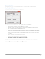
Contents
FastExcel Version 3
1 USER GUIDE .................................................................................................................... 1 Overview of FastExcel
16 FastExcel V3 Profiler: Profiling tools to find performance bottlenecks and memory usage ............................................................................................... 16 FastExcel V3 SpeedTools: Performance Improvement Tools ........................ 17 FastExcel V3 Manager: Workbook Management Tools ................................. 18 About the FastExcel User Guide and Optimizing Calculations Guide. ........................ 18 Using FastExcel Profiling: Quick Start and Drill-down Wizard
19 Do you know why your spreadsheet is slow? ............................................................. 19 Find out why then fix it with FastExcel: ......................................................... 19 How FastExcel V3 helps you run Excel faster: ............................................. 20 Full Calculation, Recalculation and Volatility: What and Why .................................... 21 Multi‐Threaded Calculation: What and Why .............................................................. 21 Step‐by‐step Drill Down to Calculation Bottlenecks ................................................... 22 Step 1: Clean and Backup your Workbook .................................................... 22 Step 2: First Drill‐down: Profile the active Workbook ................................... 22 Step 3: Second Drill‐down: Profile the worst worksheet .............................. 22 Step 4: Third Drill‐down: Drill down to individual formulas within the worst formula area ........................................................................................ 22 Step 5: Repeat steps 3 to 4 for the next worst worksheet ............................ 22 Optimizing Excel Calculation Bottlenecks
23 Use FastExcel V3 to Eliminate Calculation Bottlenecks .............................................. 24 Addressing Calculation Bottlenecks ............................................................................ 25 How fast should my spreadsheet calculate? .............................................................. 26 The Effects of Slow Response Time ............................................................... 26 What’s new in FastExcel Version 3 for FastExcel V2 Users
FastExcel V3 User Guide
27 FastExcel Version 3  2
FastExcel V3 Products ................................................................................................. 27 64‐bit and Ribbon Support ......................................................................................... 27 What’s new in FastExcel V3 Profiler for FastExcel V2 Users ....................................... 28 What’s new in FastExcel V3 Manager ......................................................................... 28 What’s new in FastExcel V3 SpeedTools for FastExcel V2 Users ................................ 29 Second Generation XLL Based Functions ....................................................... 29 Many new and powerful functions ................................................................ 29 Installing FastExcel V3
31 What you need to install FastExcel V3 ........................................................................ 31 Install package contents ............................................................................................. 31 Installing and Activating FastExcel V3
32 Buy License .................................................................................................... 34 Release All Licenses ....................................................................................... 34 Activate New License ..................................................................................... 35 To permanently uninstall FastExcel V3: ......................................................... 36 To Re‐Install FastExcel: .................................................................................. 36 Using FastExcel Functions and run‐time support ....................................................... 36 Migrating from FastExcel V2.
37 The FastExcel V3 Ribbon and Toolbars: Overview of Commands.
38 FastExcel V3: Controlling Calculation
41 FastExcel V3 Calculation Options and Settings ........................................................... 42 Excel Calculation Settings: Current Calculation Mode ................................................ 43 Excel Calculation Settings: Set Book Modes ............................................................... 45 Excel Calculation Settings: Initial Calculation Mode ................................................... 46 Excel Calculation Settings: Iteration ........................................................................... 46 Multi‐threaded calculation Settings ........................................................................... 47 Excel Calculation Settings: Calculation Buttons .......................................................... 48 FastExcel V3 User Guide
FastExcel Version 3  3
Workbook Calculation Settings ................................................................................... 50 FastExcel Settings ....................................................................................................... 55 Calculation Timing Commands
59 The seven Calculation buttons .................................................................................... 59 Getting Consistent Results from FastExcel V3 Timing ................................................ 62 Power Saving and Dual Core Intel and AMD processors: .............................. 62 Excel minimizes the number of calculations: ................................................ 62 Why FastExcel Timing results may vary from run to run: .............................. 62 Profiling Commands
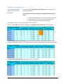
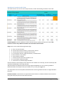
63 The Profiling Commands ............................................................................................. 63 Using the Drill‐Down Profiling Wizard ........................................................................ 65 The Profiling Header ................................................................................................... 66 The Physical Environment Table .................................................................... 66 The Workbook Settings Table. ....................................................................... 68 The Environment Counts Table ..................................................................... 69 The Calculation Settings Tables. .................................................................... 70 Profile Workbook: Profile the active Workbook and all its Worksheets. ................... 73 Choose Profile Workbook Options ................................................................ 73 The Worksheet Profiles Table. ....................................................................... 74 Worksheet Profiles Table (2) ......................................................................... 78 Worksheet Profiles Table (3) ......................................................................... 79 The Workbook Summary Table. .................................................................... 80 Profile Worksheet Areas: Details of the Formula areas on the Sheets. ..................... 82 Choose Profile Worksheet Areas Options ..................................................... 82 Worksheet Areas Profile Table ...................................................................... 83 Using the FastExcel Go To command with the Profile Worksheet Areas sheet .............................................................................................................. 84 Profile Formulas and Functions .................................................................................. 85 FastExcel V3 User Guide
FastExcel Version 3  4
Worksheet Formulas Profile Table ................................................................ 86 Using the FastExcel Go To command with the Worksheet Formulas Profile Table ................................................................................................... 87 Function Profile Table .................................................................................... 88 Map Worksheet Cross‐references. ............................................................................. 89 Worksheet Calculation Sequence Forward Cross‐reference Tables. ............. 89 Circular Worksheet Cross‐reference Paths table ........................................... 90 Memory Usage
91 Memory Used and Pivot Cache Memory Used Buttons ............................................. 91 Memory Used ............................................................................................................. 91 Pivot Cache Memory Used .......................................................................................... 91 Clean Workbook
92 Clean Workbook Options Form .................................................................................. 92 Backup Workbook before Clean .................................................................... 92 Active or All Worksheets ................................................................................ 93 Clean Used Ranges ...................................................................................................... 94 Excel’s Used Range and Last Cell ................................................................... 94 Reset Used Range .......................................................................................... 94 Clean Excess Used Range ............................................................................... 94 Delete Excess Used range .............................................................................. 94 Do Not Clean .................................................................................................. 95 Max Number of Cells per Clean Step ............................................................. 95 Buffer Rows and Columns .............................................................................. 95 Clean Workbook Options ............................................................................................ 96 Delete Temporary Files .................................................................................. 96 Close VBE Windows ....................................................................................... 96 Remove Invalid Names .................................................................................. 96 Delete Empty Worksheets ............................................................................. 96 FastExcel V3 User Guide
FastExcel Version 3  5
Remove zero height or width shapes ............................................................ 96 Remove Zero‐sized Shapes ............................................................................ 96 Clean Workbook Options (2) ...................................................................................... 97 Clean Pivot Tables .......................................................................................... 97 Remove Unused Styles .................................................................................. 97 Remove ALL styles ......................................................................................... 97 Map Styles...................................................................................................... 97 Remove Unused Number Formats ................................................................ 98 Map Number Formats ................................................................................... 98 Clean Workbook Options (3) ...................................................................................... 99 Clear Undo Memory ...................................................................................... 99 Clear Clipboard Memory ................................................................................ 99 Name Manager Professional
100 Name Manager Credits ............................................................................................. 100 Working with Name Manager .................................................................................. 100 Name Manager is Modeless ........................................................................ 101 Name Manager is Resizable ......................................................................... 101 Name Manager Splitter Bars........................................................................ 101 The Names Listbox ....................................................................................... 102 Sorting the Names Listbox ........................................................................... 102 Dividing the Space between Name and Refersto ........................................ 102 Selecting one or more Names...................................................................... 102 Refers to edit box ......................................................................................... 102 Refersto Splitter Bar .................................................................................... 103 Name Manager Filters .............................................................................................. 104 Name Scope filter ........................................................................................ 104 And/Or option buttons ................................................................................ 104 FastExcel V3 User Guide
FastExcel Version 3  6
Invert Filters ................................................................................................. 104 NameType(s) filter ....................................................................................... 104 Filter names containing Checkbox ............................................................... 104 Search Editbox ............................................................................................. 105 Unused names checkbox ............................................................................. 105 Name Manager Action Buttons ................................................................................ 106 Hide, Unhide Buttons ................................................................................... 106 Add Button ................................................................................................... 106 Delete Button ............................................................................................... 106 List Button .................................................................................................... 106 Pickup Button ............................................................................................... 106 Name Manager Action Buttons(2) ............................................................................ 107 Localise Button ............................................................................................ 107 Globalise Button .......................................................................................... 107 Evaluate Button ........................................................................................... 107 Analyze Name Button .................................................................................. 108 Highlight Button ........................................................................................... 110 Clear Button ................................................................................................. 110 Is Used ? Button ........................................................................................... 110 Refresh Button ............................................................................................. 110 GoTo button ................................................................................................. 111 GoBack button ............................................................................................. 111 Renaming a Name ........................................................................................ 111 UnName ....................................................................................................... 111 About Button ............................................................................................... 111 Dynamic Range Wizard Button .................................................................... 112 Find and Replace button .............................................................................. 112 FastExcel V3 User Guide
FastExcel Version 3  7
Name Map Button ....................................................................................... 113 Name Manager Help Button ........................................................................ 113 Name Manager Options Listbox ............................................................................... 114 Confirm Changes .......................................................................................... 114 Show Excel System Names........................................................................... 114 Show refersto............................................................................................... 114 R1C1 Notation .............................................................................................. 114 Icons ............................................................................................................. 114 Language dropdown ................................................................................................. 115 Name Manager and the VBE ..................................................................................... 115 Reset NM
115 Corrupt names .......................................................................................................... 116 Problems discovered during the development of this utility ................................... 117 Non US List separators ................................................................................. 117 Unusual Characters in Names ...................................................................... 117 Duplicate Global Local Names ..................................................................... 117 Names with refers‐to starting with =! ......................................................... 117 Dynamic Range Wizard
119 Creating Dynamic Range Names ............................................................................... 119 Starting the Dynamic Range Wizard ............................................................ 119 Dynamic Range Wizard Step 1 ..................................................................... 119 Dynamic Range Wizard Step 2 ..................................................................... 120 Step 2A: Choose Dynamic Expansion Method ............................................. 120 Step2B: Select the Anchor Cell .................................................................... 120 Dynamic Range Wizard Step 3 ..................................................................... 121 Dynamic Range Wizard Step 4 ..................................................................... 123 Dynamic Range Wizard Step 5 ..................................................................... 126 FastExcel V3 User Guide
FastExcel Version 3  8
Indenting Formula Viewer, Editor and Debugger V2
128 Formula Box .............................................................................................................. 130 Left‐Click in the Formula Box ....................................................................... 130 Double‐Click in the Formula Box ................................................................. 130 Right‐Click in the Formula Box ..................................................................... 130 F9 in the Formula Box .................................................................................. 130 Splitter Bar ................................................................................................................ 130 Description Area ....................................................................................................... 130 Evaluation Box .......................................................................................................... 130 Resizing the Form ..................................................................................................... 131 Origin Destination ..................................................................................................... 131 View and Edit Modes ................................................................................................ 132 Active Origin Mode ...................................................................................... 132 Constant Origin Mode ................................................................................. 132 Edit Mode .................................................................................................... 132 Indent style ............................................................................................................... 133 Change Selection ...................................................................................................... 133 Shift and/or Control ..................................................................................... 133 Alt ................................................................................................................. 133 Back and Next ........................................................................................................... 133 Undo Redo and Refresh ............................................................................................ 134 Undo Redo ................................................................................................... 134 Refresh ......................................................................................................... 134 Print........................................................................................................................... 134 View/Edit Shortcut and Function Keys ..................................................................... 135 Additional Edit Mode Buttons .................................................................................. 136 Destination Formula Address ...................................................................... 136 Unformat/Reformat ..................................................................................... 136 FastExcel V3 User Guide
FastExcel Version 3  9
Adding or changing Functions, References and Defined Names. ............................. 137 Add Reference ............................................................................................. 137 Function Wizard ........................................................................................... 137 Insert Name ................................................................................................. 138 Clear ............................................................................................................. 138 This button will remove all the text from the formula box. ........................ 138 Copy From .................................................................................................... 138 Changing a reference from relative to absolute .......................................... 139 Enter Formula ........................................................................................................... 139 Settings ..................................................................................................................... 140 Initial Indent Style ........................................................................................ 140 Scroll GoTo ................................................................................................... 140 Unhide Hidden GoTos .................................................................................. 140 Evaluate and Description Settings ............................................................... 141 Edit Mode Array Formula Handling: ............................................................ 142 Sheet Manager
143 Workbook Name ....................................................................................................... 144 Sheets Box ................................................................................................................. 144 Sheet Manager Action Buttons ................................................................................. 145 Hide Unhide ................................................................................................. 145 Protect Unprotect ........................................................................................ 145 Activate ........................................................................................................ 145 Refresh ......................................................................................................... 145 Rename ........................................................................................................ 145 Delete ........................................................................................................... 145 Insert or Copy Before or After ..................................................................... 146 Mix Mode Settings ....................................................................................... 146 FastExcel V3 User Guide
FastExcel Version 3  10
Mixed Mode On or OFF ............................................................................... 146 Move Up Move Down .................................................................................. 147 Sort Workbook Sheets .............................................................................................. 147 Choose Sheet Filters ................................................................................................. 148 And Or Invert Filters .................................................................................................. 148 Available Sheet Filters ............................................................................................... 149 SpeedTools Overview
150 High‐Performance, High‐Power Functions ............................................................... 151 Extend your capabilities with over 90 High‐Power Functions .................................. 152 High‐Performance AVLOOKUP2 family of functions ................................................. 154 Regular Expression Functions ................................................................................... 154 High‐Performance FILTER.IFS family of functions..................................................... 155 The Family of LISTDISTINCT Functions ...................................................................... 157 New Family of AND and OR functions designed for Array Formulas. ....................... 157 5 New functions to simplify and extend array‐handling........................................... 157 10 New Text‐handling Functions .............................................................................. 157 6 Dynamic sorting functions ..................................................................................... 157 New Math and Statistics functions ........................................................................... 158 New Calculation Methods & Properties ................................................................... 159 Extended Calculation Modes .................................................................................... 159 Getting Started with FastExcel SpeedTools
160 The Excel 2003 SpeedTools Toolbar ......................................................................... 160 SpeedTools Functions
161 Excel Function Wizard ............................................................................................... 161 SpeedTools Functions by Product and Category ...................................................... 164 SpeedTools Functions Properties ............................................................................. 166 SpeedTools Filters: Filtering Functions
168 The FILTER.IFS Multiple Criteria Function Family ..................................................... 169 FastExcel V3 User Guide
FastExcel Version 3  11
FILTER.IFS function .................................................................................................... 171 FILTER.IFS and ASUMIFS Examples ........................................................................... 178 FILTER.SORTED function ........................................................................................... 181 FILTER.MATCH function ............................................................................................ 182 FILTER.MATCH Example ............................................................................................ 182 ASUMIFS function ..................................................................................................... 183 ACOUNTIFS function ................................................................................................. 184 FILTER.VISIBLE function ............................................................................................ 185 Rgx.COUNTIF function .............................................................................................. 186 Rgx.SUMIF function .................................................................................................. 187 The LISTDISTINCTS family of functions. .................................................................... 188 LISTDISTINCTS Function ............................................................................................ 189 LISTDISTINCTS.COUNT Function ............................................................................... 191 LISTDISTINCTS.SUM Function ................................................................................... 192 LISTDISTINCTS.AVG Function .................................................................................... 193 COUNTDISTINCTS Function ....................................................................................... 194 COUNTDUPES Function ............................................................................................. 195 LISTDISTINCTS Examples ........................................................................................... 196 SpeedTools Filters - Sorting Functions
199 VSORTC – Dynamic text collating Sort of a vertical range or array .......................... 201 Case.VSORTC – Case‐sensitive dynamic Sort of a vertical range or array ................ 202 VSORTB – Fast Dynamic Sort of a vertical range or array ......................................... 203 VSORTC.INDEX – Collating Text Index Sort of a vertical range or array ................... 204 Case.VSORTC.INDEX – Collating Text Index Sort of a vertical range or array ........... 205 VSORTB.INDEX – Fast Index Sort of a vertical range or array ................................... 206 SpeedTools Lookups: Lookup Functions
207 Outstanding Performance ........................................................................................ 207 Advanced Function ................................................................................................... 207 FastExcel V3 User Guide
FastExcel Version 3  12
Better, Safer Lookup Defaults ................................................................................... 208 SpeedTools Lookup Families ..................................................................................... 208 High‐performance exact match Memory Lookups ................................................... 209 Reconciling lists super‐fast using COMPARE.LISTS ................................................... 211 The 24 Advanced Function Lookups ......................................................................... 211 MEMLOOKUP Function ............................................................................................. 213 MEMMATCH Function .............................................................................................. 216 COMPARE.LISTS Function ......................................................................................... 219 COMPARE.LISTS Examples ........................................................................................ 221 AVLOOKUP2, AVLOOKUPS2 & AVLOOKUPNTH Functions ........................................ 224 AVLOOKUP2 Examples .............................................................................................. 228 Case.AVLOOKUP2, Case.AVLOOKUPS2 & Case.AVLOOKUPNTH Functions .............. 232 AMATCH2, AMATCHES2 & AMATCHNTH functions ................................................. 236 Case.AMATCH2, Case.AMATCHES2 & Case.AMATCHNTH functions ........................ 240 Rgx.AVLOOKUP2, Rgx.AVLOOKUPS2 & Rgx.AVLOOKUPNTH Functions ................... 244 Rgx.Case.AVLOOKUP2, Rgx.Case.AVLOOKUPS2 & Rgx.Case.AVLOOKUPNTH Functions ................................................................................................................... 247 Rgx.AMATCH2, Rgx.AMATCHES2 & Rgx.AMATCHNTH functions ............................. 250 Rgx.Case.AMATCH2, Rgx.Case.AMATCHES2 & Rgx.Case.AMATCHNTH functions ... 253 EVAL2 function: evaluate a string ............................................................................. 256 SpeedTools Extras: Mathematical Functions
257 VLINTERP2 function .................................................................................................. 258 LINTERP2D function .................................................................................................. 260 Calculating Gini Coefficients with GINICOEFF ........................................................... 261 GINICOEFF function .................................................................................................. 262 SpeedTools Extras: Logical Functions
263 SpeedTools Logical Functions for Array Formulas .................................................... 264 FastExcel V3 User Guide
FastExcel Version 3  13
OR.ROWS, OR.COLS, OR.CELLS, AND.ROWS, AND.COLS, AND.CELLS, ALL, ANY, NONE ......................................................................................................................... 264 Examples of SpeedTools Logical Functions: .............................................................. 265 IFERRORX Function ................................................................................................... 269 SpeedTools Extras: Reference Functions
271 PREVIOUS Function ................................................................................................... 272 SETMEM and GETMEM Functions ............................................................................ 274 SpeedTools Extras: Array-Handling Functions
275 COL.ARRAY Function ................................................................................................. 276 ROW.ARRAY Function ............................................................................................... 278 REVERSE.ARRAY Function ......................................................................................... 280 PAD.ARRAY Function ................................................................................................. 282 VECTOR Function ...................................................................................................... 284 SpeedTools Extras: Information Functions
285 HASFORMULA2 function ........................................................................................... 286 Calculation Sequence and Counting functions ......................................................... 287 CALCSEQCOUNTREF Function ................................................................................... 287 CALCSEQCOUNTSET Function ................................................................................... 287 CALCSEQCOUNTVOL function ................................................................................... 287 Functions for counting Rows and Columns .............................................................. 288 COUNTROWS2 Function ........................................................................................... 289 COUNTCONTIGROWS2 Function .............................................................................. 291 COUNTUSEDROWS2 Function .................................................................................. 293 COUNTCOLS2 Function ............................................................................................. 294 COUNTCONTIGCOLS2 Function ................................................................................ 296 COUNTUSEDCOLS2 Function .................................................................................... 298 Examples and comparison of the counting functions .............................................. 298 Using the Count functions in dynamic range names ............................................... 299 FastExcel V3 User Guide
FastExcel Version 3  14
SpeedTools Extras: Text Functions
300 CONCAT.RANGE – concatenate range data .............................................................. 301 PAD.TEXT function .................................................................................................... 302 REVERSE.TEXT Function ............................................................................................ 303 SPLIT.TEXT Function .................................................................................................. 304 GROUPS Function ..................................................................................................... 305 Rgx.FIND function ..................................................................................................... 308 Rgx.LEN function ....................................................................................................... 309 Rgx.SUBSTITUTE function ......................................................................................... 310 Rgx.MID function ...................................................................................................... 311 COMPARE function ................................................................................................... 312 ISLIKE2 array function for pattern‐matching strings ................................................ 313 Rgx.ISLIKE function .................................................................................................... 314 FastExcel V3 Help
316 Using FastExcel V3 with VBA
317 Calling SpeedTools functions from VBA .................................................................... 317 Measuring Macro execution time ............................................................................. 318 Timing User Defined Functions ................................................................................. 318 Using FastExcel V3 calculation methods from VBA .................................................. 319 MICROTIMER function .............................................................................................. 320 MILLITIMER function ................................................................................................. 320 STRCOLID function .................................................................................................... 321 Using MICROTIMER from VBA .................................................................................. 322 FastExcel V3 User Guide
FastExcel Version 3  15
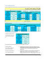
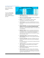
OverviewofFastExcel
FastExcel gives you a wide variety of tools to analyze, manage, control and optimize the performance and memory usage of your workbooks. These tools fall into the following groups: FastExcelV3Profiler:Profilingtoolstofindperformancebottlenecksandmemoryusage

Drill‐down Wizard 
Profile Workbook 
Profile Worksheet Areas 
Profile Worksheet Formulas and Functions 
Range Calculate to time calculation of a small block of formulas. 
Map Worksheet Sequence: This command looks at the flow of calculations between worksheets. 
Calculate Range 
Calculate Sheet 
Calculate Workbook 
Time a Macro FastExcelV3Profiler:TimingTools
These tools can be used during development and optimization of a workbook to quickly compare the calculation speeds of different formulas, worksheets etc., and, with large slow workbooks, allow you to quickly calculate a small subset of the workbook. FastExcelV3Profiler:MemoryTools

Workbook Memory Used 
Pivot Cache Memory Used These tools show you the memory used by your workbooks and pivot tables. FastExcel V3 User Guide
Overview of FastExcel  16
FastExcelV3SpeedTools:PerformanceImprovementTools

Additional Calculation Modes Excel only has two calculation modes (Automatic and Manual) to apply to all the open workbooks and worksheets, and all the open workbooks are calculated at each calculation. This can be slow and inconvenient when you have multiple workbooks open or one or more of the worksheets in your workbook only need calculating infrequently. FastExcel allows you to calculate only the active workbook, to set different calculation modes for each workbook, and to control when the individual worksheets in a workbook are calculated. 
Advanced SpeedTools Functions SpeedTools provides an extensive library of over 80 multi‐threaded worksheet functions which you can use to speed up many slow calculations. FastExcel V3 User Guide
Overview of FastExcel  17
FastExcelV3Manager:WorkbookManagementTools

Clean Workbook: Clean workbook gives you a comprehensive set of tools for eliminating wasted space and maintaining your workbooks. 
View/edit/debug Formulas: Edit and view complex formulas using a variety of indentation and selection methods. Easy handling of embedded functions. 
Sheet Manager: Sheet Manager provides an easy way of managing a large number of sheets in a workbook. 
Name Manager Pro: Name Manager Pro greatly simplifies management and maintenance of Excel Defined Names. AbouttheFastExcelUserGuideandOptimizingCalculationsGuide.
The FastExcel User Guide has 3 main sections. 
The Introduction provides you an overview of FastExcel. 
The Quick Start Guide gives you a fast way of getting started and seeing some results before you delve into the more intricate details. 
The remainder of the User Guide is a reference manual to all the features of FastExcel. The companion Optimizing Excel Calculations and Memory guide has 4 main sections: 
Bottlenecks 
Optimizing Tips and Tricks 
Excel Calculation Information 
Excel Memory All of this material is available both as online help (FastExcel Help and Contextual help) and as viewable and printable PDF manuals. You can find the PDF manuals in the directory where FastExcel was installed (usually C:/Program Files/FastExcelV3). FastExcel V3 User Guide
Overview of FastExcel  18
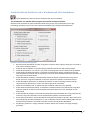
UsingFastExcelProfiling:QuickStartandDrill‐downWizard
To make the best of the Drill‐down wizard it’s a good idea to read some background material on profiling Excel calculations. Doyouknowwhyyourspreadsheetisslow?

Which of your worksheets is using the calculation time? 
Which of your formulas is using the calculation time? 
Do you have too many volatile formulas? 
Where are your volatile formulas? 
Are your lookups or array formulas running slow? 
Are you properly exploiting Excel’s multi‐threaded calculation engine? 
Have you got a memory usage problem? 
Or a used‐range problem? 
Do you need better control of what gets recalculated? 
How much of your time is each of these problems taking? FindoutwhythenfixitwithFastExcel:
Speed up Excel with FastExcel V3. 
Drill down and locate your calculation bottlenecks. 
Prioritize bottlenecks by time consumption. 
Find out how volatility is affecting your calculation time. 
Measure your multi‐threaded efficiency and locate the functions that are not multi‐threaded. 
Solve calculation problems with SpeedTools fast functions. 
Build efficient spreadsheets. 
Document and compare calculation efficiency and memory usage. 
Time your User Defined Functions. 
Compare alternative Excel formulas FastExcel V3 User Guide
Using FastExcel Profiling: Quick Start and Drill-down Wizard  19
HowFastExcelV3helpsyourunExcelfaster:
You can speed up your Spreadsheet by finding and eliminating calculation bottlenecks FastExcel V3 helps you find and prioritize bottlenecks Most slow‐running spreadsheets contain a small number of problem areas, or Bottlenecks. Because Excel is such a flexible spreadsheet system there are usually many different formulas that can produce the answer you want. Some of these formulas are much faster than others, and SpeedTools gives you faster alternatives for many functions. In large spreadsheets it can be difficult to locate and prioritize the Bottlenecks. You can use the Drill‐down wizard and the wide variety of timing and profiling tools in FastExcel to rapidly drill down, locate and prioritize these bottlenecks, and then use SpeedTools extensive function library to find faster‐calculating solutions. Help and advice on optimizing bottlenecks is just a click away with FastExcel’s built‐in Contextual Help, and is also available in the Optimizing Excel Calculations and Memory manual. FastExcel V3 User Guide
Using FastExcel Profiling: Quick Start and Drill-down Wizard  20
FullCalculation,RecalculationandVolatility:WhatandWhy
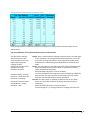
To get the best out of FastExcel you need to understand the difference between an Excel Recalculation, where Excel works out how to recalculate the smallest number of formulas possible, and an Excel Full Calculation, where Excel calculates every single formula regardless of whether it has already been calculated or not. Volatile formulas get recalculated at every calculation. Which of these types of calculation is more important for you depends on how much of the input data changes each time you want to calculate the workbook, and how many volatile formulas you have. FastExcel V3 Profiler will measure the volatility of each worksheet and can identify which built‐in and XLL based functions are volatile. For example if you are doing a monthly budget variance analysis each month most of the input data will change and almost all the formulas will need to be recalculated. But if you are doing a what‐if analysis on a cash‐flow model then you may change only a single input number that will cause only a small number of the formulas to be recalculated. If possible you should decide which of these two scenarios is the most likely for your workbook, because it can significantly affect which part of your FastExcel Profiling analysis is most significant for you, and also the methods you use to optimize your workbook calculations. Multi‐ThreadedCalculation:WhatandWhy
In Excel 2007 the Excel calculation engine was rewritten to use all the available cpus/cores in your PC. This method of multi‐threaded calculation can have a dramatic effect on your Excel calculation times: on a 4‐core PC a well‐designed workbook can run up to 4 times faster than with single‐threaded calculation. But some worksheet functions (all VBA user‐defined functions and many add‐in library functions) are single‐threaded and so will seriously slow down calculation. FastExcel V3 Profiler will measure the multithreaded efficiency both of the individual worksheets and the overall workbook, and can identify any single‐threaded functions being used. FastExcel V3 User Guide
Using FastExcel Profiling: Quick Start and Drill-down Wizard  21
Step‐by‐stepDrillDowntoCalculationBottlenecks
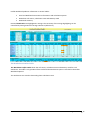
If you would like to get some immediate results on your workbooks without delving into lots of details you can simply use the Drill‐down Wizard to find the Calculation Bottlenecks. Once you are more familiar with some of FastExcel's features you can use the online help and FastExcel manuals to investigate additional ways of finding and eliminating bottlenecks. Step1:CleanandBackupyourWorkbook
Be sure to back up your workbook before you start Back up your workbook using Clean Workbook and use the commands to remove unnecessary items and wasted space from your workbook. Step2:FirstDrill‐down:ProfiletheactiveWorkbook
Find the problem
worksheets, volatility and
multi-threading
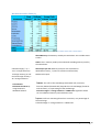
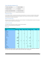
inefficiencies The first time you click the Drill‐down wizard button it profiles the active workbook to find and prioritize:  The calculation times for each worksheet.  Workbook and worksheet Volatility and multi‐threaded efficiency
 Used Range wastage by worksheet. Note: when using the Trial version of FastExcel V3 Drill Down will only profile a single worksheet. Step3:SecondDrill‐down:Profiletheworstworksheet
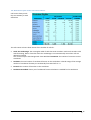
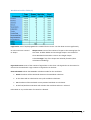
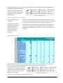
Find the problem formula
blocks on the worst
worksheet. With the FastXLBook result sheet active click the Drill‐down Wizard to profile the worst worksheet to find and prioritize the calculation time for blocks of formulas. The Drill‐down wizard will automatically pick the worst worksheet unless you select a different worksheet result row. Step4:ThirdDrill‐down:Drilldowntoindividualformulaswithintheworstformulaarea
Find the worst formulas
within the worst area on
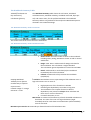
the worst sheet With the FastXLSheet result sheet active click the Drill‐down wizard to drill down into the formulas in the worst formula area block. Step5:Repeatsteps3to4forthenextworstworksheet
With the FastXLBook result sheet active select the next worst worksheet result row and click the Drill‐down Wizard to repeat the process. Note: when using the Trial version of FastExcel V3 Drill Down will only profile a single worksheet. FastExcel V3 User Guide
Using FastExcel Profiling: Quick Start and Drill-down Wizard  22
OptimizingExcelCalculationBottlenecks
Most Excel spreadsheets contain a number of calculation bottlenecks. Some of the most common bottlenecks are: FastExcel V3 User Guide

Exact Match Lookup using MATCH, VLOOKUP, and HLOOKUP: Excel has to scan through each row of the data table until it finds a match. This can be very slow for large tables. 
Array Formulas and SUMPRODUCT: Using Array formulas and SUMPRODUCT can do amazing things, but forces Excel to do many calculations, which often results in slow calculations. 
Excel calculating more than you need: you can use FastExcel to more precisely control which parts of your workbooks should be calculated. 
SUM, SUBTOTAL, SUMIF, and COUNTIF: These formulas can make Excel scan a large number of cells. 
Single‐threaded Functions: Using single‐threaded worksheet functions can slow down calculation by a large factor. 
User‐Defined Functions: There are significant overheads involved in calling VBA UDFs and in transferring data from Excel to the UDF. With care these overheads can be minimized. 
Volatile Functions: Using volatile functions means that Excel cannot get the best out its smart recalculation engine so that each recalculation takes longer. 
Conditional Formats: A large number of conditional formats can significantly slow workbook calculation. 
Large Ranges: Using larger ranges than necessary can be expensive for calculation time. 
Duplicated calculations: it is very easy to build a spreadsheet where many of the calculations are being repeated many times. 
Workbook Links: Links to other workbooks are slow and fragile. Optimizing Excel Calculation Bottlenecks  23
UseFastExcelV3toEliminateCalculationBottlenecks
Once you have identified and prioritized the calculation bottlenecks you can set about eliminating and reducing them: SlowLookupsandMatches

Use SpeedTools's advanced memory lookup technology to speed up recalculation of exact match lookups. 
Sort the data and use SpeedTools super‐fast sorted exact match lookup. 
SpeedTools MEMMATCH, MEMLOOKUP, AVLOOKUP2 and AMATCH2 all use memory lookup and sorted exact match lookup 
Use SpeedTools AVLOOKUP2 and AMATCH2 built‐in exact match error handling 
Handle multiple‐condition lookups efficiently with SpeedTools AVLOOKUP2 and AMATCH2 rather than using slow array formulas or concatenation SlowArrayFormulasandSUMPRODUCTformulas

Use SpeedTools FILTER.IFS powerful and efficient multiple condition handling to replace slow SUMPRODUCT and array formulas. 
Sort your data and use SpeedTools FILTER.IFS ability to exploit sorted data efficiently 
Minimize the effective size of the ranges you are using with FastExcel Managers Dynamic Range Wizard (part of FastExcel V3 Name Manager Pro) EliminateUnnecessaryCalculations

Use FastExcel V3 Calc’s extended calculation options to control exactly which parts of your spreadsheets should be calculated. 
Look for duplicated calculations in formulas or parts of formulas and break them out into a separate column so that they only have to be done once. SlowVBAUDFs

Installing FastExcel V3 Calc will bypass Excel’s VBE UDF refresh bug and speed up calculation when you have a large number of VBA UDFs. 
SpeedTools powerful and extensive range of functions may be able to replace some of your VBA UDFs Look at the Optimizing Excel Calculations and Memory manual, or click FastExcel Contextual Help for more details and advice. FastExcel V3 User Guide
Optimizing Excel Calculation Bottlenecks  24
AddressingCalculationBottlenecks
Once you have identified the calculation bottlenecks you can use FastExcel to help you reduce or eliminate them: Tune‐up your spreadsheet with FastExcel. FastExcel Contextual Help Find all the cells with the same Number Format or Style Use the Clean Workbook or Where‐Used command to create Maps of where the Number Formats and Styles are being used FastExcel V3 User Guide

Select a cell containing a problem formula and use FastExcel’s Contextual Help or Speedup Help for advice on how to improve common bottlenecks. 
Use the CrossRef command to find improved worksheet calculation sequences. 
Access FastExcel’s advice on removing unnecessary calculations.

Choose the best calculation options for your spreadsheet, using FastExcel's extended calculation methods. 
Use FastExcel’s built‐in Contextual Help. 
On an ordinary Excel worksheet Contextual help shows you Speedup help, where possible relating to the functions used in the active cell. 
On a FastExcel output sheet FastExcel help shows you help for the nearest information block. Use the FastExcel GoTo command to select all cells on the active sheet with the same Number Format or Style as the currently selected cell. When the active sheet is a Number Format Map sheet or Style Map sheet created by the Clean Workbook or Where‐used Map commands, the GoTo command will use the selected cell on the map to 
Select the corresponding sheet 
Select all the cells on that sheet with the corresponding Number Format or Style. Optimizing Excel Calculation Bottlenecks  25
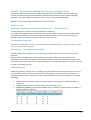
Howfastshouldmyspreadsheetcalculate?
Studies on the effects of slow response time (see below) show that there are two ‘comfort zones’ of calculation times for users: 
For calculation times of less than about a tenth of a second users feel comfortable with Automatic Calculation. 
For calculation times of up to about 10 seconds in Manual Calculation mode users can maintain concentration and avoid errors. So wherever possible you should try to use FastExcel to get your workbook calculation speed into one of these comfort zones. TheEffectsofSlowResponseTime
Research studies show that a user’s productivity and ability to focus on the task deteriorate as response time lengthens. 
Response time greater than 10 seconds: Users generally refuse to wait longer than 10 seconds 
Response time greater than 1 second but less than 10 seconds: User errors, and annoyance level, start to increase, particularly for repetitive tasks 
When response time is longer than 10 seconds users tend to switch to other tasks. When response time is less than 10 seconds but longer than 1 second the user has difficulty in retaining a train of thought, but will probably not have switched to doing a different task whilst they are waiting. Sub‐Second Response: Improving calculation speed to less than a second increases productivity For response times greater than a tenth of a second but still less than about 1 second, users can successfully keep a train of thought going, although they will notice the response time delay. IBM studies from the 1970s and 1980s showed significant productivity gains for users when response times were less than a second. You will probably need to switch to Manual Calculation mode when entering data. 
Instant response You can use Automatic Calculation Mode even when entering data FastExcel V3 User Guide
For response times of less than about a tenth of a second, users feel that the system is responding instantaneously. Optimizing Excel Calculation Bottlenecks  26
What’snewinFastExcelVersion3forFastExcelV2Users
Useful information for users upgrading from FastExcel Version 2. FastExcelV3Products
FastExcel has been split into 6 separately available products so that you only need to purchase the products you need. 
FastExcel V3 Profiler 
FastExcel V3 Manager 
FastExcel V3 SpeedTools Calc (FastExcel run‐time engine) 
FastExcel V3 SpeedTools Lookups 
FastExcel V3 SpeedTools Filters 
FastExcel V3 SpeedTools Extras There also 2 product bundles available 
FastExcel V3 Bundle, which includes all 6 products 
FastExcel V3 SpeedTools Bundle, which includes all the 4 SpeedTools products You also get a free copy of SpeedTools Calc when you buy any other FastExcel V3 product. 64‐bitandRibbonSupport
All FastExcel V3 products support both 32‐bit and 64‐bit Excel. All FastExcel V3 products support both the Ribbon and Toolbars user interfaces FastExcel V3 User Guide
What’s new in FastExcel Version 3 for FastExcel V2 Users  27
What’snewinFastExcelV3ProfilerforFastExcelV2Users

Supports both Excel 32 and 64 bit versions 
Supports Excel 2003 through Excel 2013 
Both Ribbon and Toolbar user interfaces 
Drill‐down Profiling wizard for easy and fast profiling 
Profiles Multi‐Threaded Calculation efficiency 
New Profile Formulas and Functions command can profile down to unique formulas on a worksheet. 
Faster profiling 
Increased control over what gets profiled and the profiling tests performed 
More information and statistics 
XLB and QUAT sizes 
Com Addins and XL addins 
Force Full Calculation 
Workbook Calculation Engine 
Windows and Excel Versions details 
Multi‐Threaded Calculation Status 
Conditional Formats Statistics 
Worksheet Calculation Mode What’snewinFastExcelV3Manager







Indented formula editor/viewer/debugger Sheet Manager Name Manager Pro supports both Tables and Defined Names Choice of INDEX or OFFSET for the Dynamic Range Wizard Remove all styles option for Clean Workbook Where‐used Mapping of Styles, Number Formats and Defined Names Simplified GoTo selection of styles and number formats from the where‐used Maps FastExcel V3 User Guide
What’s new in FastExcel Version 3 for FastExcel V2 Users  28
What’snewinFastExcelV3SpeedToolsforFastExcelV2Users
Run‐timeforFastExcel
FastExcel V3 SpeedTools Calc contains in one convenient family of products all the FastExcel components required to enable both the additional FastExcel calculation modes and the FastExcel SpeedTools high‐
performance functions. The FastExcel Profiling functions and workbook management tools are available in other FastExcel products. SecondGenerationXLLBasedFunctions
All FastExcel V2 UDFs such as AVLOOKUP and AMATCH have been replaced by a second generation of XLL‐based functions. This provides: 
Improved Function wizard support 
You can easily move workbooks containing the functions between different PCs even when FastExcel V3 is installed in different locations. 
Most FastExcel V3 functions are multi‐threaded 
Improved lookup Memory technology is retained in saved workbooks Manynewandpowerfulfunctions
SpeedTools includes over 80 new Excel Functions: 
A family of FILTER.IFS functions for efficient replacement of multiple conditions array and SUMPRODUCT formulas 
More powerful LOOKUP and MATCH functions 
A family of efficient DISTINCT, UNIQUE and SORT functions 
Very fast COMPARE.LISTS functions 
Array handling and stacking functions 
Regular Expression functions 
Case sensitive functions 
Text handling functions 
Information functions FasterFunctions
Most SpeedTools functions are now multi‐threaded and fully compiled in C++ giving faster performance, especially in Automatic Calculation mode. FastExcel V3 User Guide
What’s new in FastExcel Version 3 for FastExcel V2 Users  29
Full‐columnreferences
Most SpeedTools functions efficiently handle full‐column references. ImprovedaccuracyofcalculationTimingCommands
The FastExcel Range calculation timing commands have been extended to allow you to specify the number of timing trials you want to perform. Accuracy is improved by automatically discarding high and low timings. This is particularly important for timing calculate of very small numbers of formulas where Windows multi‐tasking can easily disrupt a single timing. FastExcel V3 User Guide
What’s new in FastExcel Version 3 for FastExcel V2 Users  30
InstallingFastExcelV3
Information to help you install FastExcel V3 successfully. WhatyouneedtoinstallFastExcelV3

The Downloaded FastExcel V3 Install file. 
Excel 2003 or later 
Administrator Rights 
Adobe Acrobat Reader 4.0 or later to view or print the manuals. Installpackagecontents
FastExcel V3 User Guide

The FastExcel V3 programs. 
FastExcel V3 user guide and help files. 
Optimizing Calculations manual and help files. 
Automatic Install/Uninstall. Installing FastExcel V3  31
InstallingandActivatingFastExcelV3
Prerequisites
FastExcel V3 requires: 
Excel 2003, Excel 2007, Excel 2010 (32 or 64 bit), Excel 2013 (32 or 64 bit) 
Windows XP, Windows Vista, Windows 7 or Windows 8 
Installation requires administrative privileges Installation
You can download the latest build of FastExcel V3 from the Decision Models website You will need to unzip the file containing the installer. Installation requires administrative privileges. Running the installer will create a folder to contain all the FastExcel V3files. The default directory is called FastExcel V3 and is located in your Program Files directory. You can choose a different install folder during the installation process. The folder will contain the XLA, XLAM and XLL files needed to run SpeedTools. Help files (.CHM) and a PDF version of this guide will also be installed in this folder. After successful installation FastExcel V3 will automatically be started when you start, and you will find FastExcel V3 on the main Ribbon Tab. If the Ribbon does not show the FastExcel V3 tab, or the installation was done for you by another user with administrative privileges, you may have to use Excel to install the FastExcel V3 XLA file: For Excel 2003 and earlier, go to Tools‐>Addins For Excel 2007 Click Office Button‐>Excel Options‐>Addins‐>Excel Addins‐>Go… For Excel 2010 and 2013 Click File‐>Excel Options‐>Addins‐>Excel Addins‐>Go… 
Press Browse and locate the folder containing FastExcel V3. 
Select the FastExcelV3.xla file and click OK to return to the Addins form. 
If asked “Do you want to copy this Addin to the Addins folder?” reply NO. 
The Excel Addins form should now show FastExcel V3 with a checkmark. Click OK to finish. UninstallingFastExcelV3
To permanently uninstall FastExcel V3 use Windows Control Panel Programs and Features. To temporarily uninstall FastExcel V3 use the Excel Addins menu (location as above) to uncheck the FastExcel V3 addin. FastExcel V3 User Guide
Installing and Activating FastExcel V3  32
TrialVersionandActivation
By default installing FastExcel V3 creates a trial version. When you start Excel using the trial version FastExcel V3 will remind you how many days of trial you have left. You can convert the trial version to a fully licensed version by entering a previously purchased activation code. The activation code can be for any of the 8 FastExcel V3 products: 
FastExcel V3 Bundle (All FastExcel V3 products) 
FastExcel V3 Profiler 
FastExcel V3 Manager 
SpeedTools Premier Bundle (All SpeedTools products) 
SpeedTools Lookups 
SpeedTools Filters 
SpeedTools Extras 
SpeedTools Calc Any combination of trial and full licenses is allowed. SpeedTools Calc may be purchased individually when required as the run‐time for the FastExcel additional calculation modes, but is also bundled with all other FastExcel V3 products. FastExcel V3 User Guide
Installing and Activating FastExcel V3  33
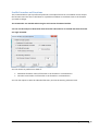
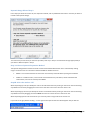
FastExcelV3LicensingSettings
You can access the FastExcel V3 licensing settings from either the License button on the FastExcel tab, or from the FastExcel V3 Ribbon‐> FastExcel Calculation Control‐>Calculation Options button, and selecting the FastExcel Settings Tab. Show License Status shows you the status of your licenses for all FastExcel V3 products. BuyLicense
Buy License takes you to the FastExcel product store where you can purchase FastExcel licenses. ReleaseAllLicenses
Use Release All Licenses when you want to move FastExcel V3 to a different machine. The command will remove all the licenses from this machine so that you can re‐activate them elsewhere. Make sure you have taken a note of the Activation license keys! FastExcel V3 User Guide
Installing and Activating FastExcel V3  34
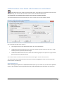
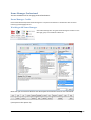
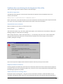
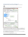
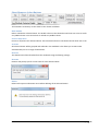
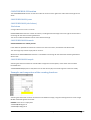
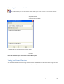
ActivateNewLicense
Add New License/Activate New License asks which product you want to add a license for: Choose the product for which you want to add a license and you will be prompted for the License Activation key. FastExcel V3 User Guide
Installing and Activating FastExcel V3  35
TopermanentlyuninstallFastExcelV3:
The Uninstall will permanently remove FastExcel V3 from your system Use the Windows Control Panel… Add/remove Programs to run the FastExcel V3uninstall package and remove FastExcel V3 from your system. ToRe‐InstallFastExcel:

If you need to re‐install FastExcel V3for any reason just double‐click your downloaded FastExcel V3 installation package. UsingFastExcelFunctionsandrun‐timesupport
If you create a workbook that uses one or more of the SpeedTools functions, or one of the new FastExcel calculation modes such as Active Workbook mode or MixedMode sheets, your workbook will not function correctly unless the required components of FastExcel V3 are installed for the copy of Excel you are using. SpeedTools Calc supports the additional calculation modes and the run‐time functions for the Dynamic Range Wizard. If you are using some of the SpeedTools functions you will require one or more of SpeedTools Filters, SpeedTools Lookups or SpeedTools Extras. The FastExcel V3 Bundle includes all FastExcel V3 components, and the SpeedTools bundle includes Calc, Filters, Lookups and Extras. FastExcel V3 User Guide
Installing and Activating FastExcel V3  36
MigratingfromFastExcelV2.
Both FastExcel V2 and FastExcel V3 can be installed on the same system whilst testing and migrating workbooks, but it would be better to uninstall FastExcel V2 once this period is over. Workbooks that use any FastExcel V2 functions such as COUNTROWS or AVLOOKUP in formulas need to have the formulas changed to use COUNTROWS2 and AVLOOKUP2 etc. Workbooks using FastExcel V2 extended calculation modes should run happily with FastExcel V3. FastExcel V3 User Guide
Migrating from FastExcel V2.  37
TheFastExcelV3RibbonandToolbars:OverviewofCommands.
In Excel 2007 and later FastExcel V3 shows and additional tab on the main Ribbon. The FastExcel V3 Ribbon shows all the FastExcel V3 commands even if not all the FastExcel V3 products are installed or licensed. In Excel 2003 FastExcel V3 shows 3 Toolbars, one each for Profiler, Manager and SpeedTools ExtendedExcelandFastExcelCalculationOptions:
Calculation Options for Excel, the Active Workbook and FastExcel. Includes Initial Mode, Mixed Mode and Active Book Calculation Modes. Show and change FastExcel V3 licensing options. The FastExcel Calculation Options button allows you to control both Excel and FastExcel Calculation settings. CalculateandTimeCommands:
The FastExcel calculate and time commands show you the time taken to do the calculation. Calculate range, Recalculate selected sheets, Full calculate Sheet, Recalculate workbooks, Full calculate workbooks and Recalculate MixMode sheets and workbooks. TimeMacroandGoToCommands:
Time Macro execution and go to Names, Cells with specified Number Formats or Styles. Time the execution of a macro, quickly select all the cells on a worksheet with a specified Style or Number Format, Goto a Name or reverse the last GoTo. ProfilingCommands:
The FastExcel profiling commands allow you to find calculation bottlenecks and memory usage. FastExcel V3 User Guide
Drill‐Down Profiling Wizard, Profile Workbook, Profile Worksheet Areas, Profile Formulas and Functions, Map worksheet cross‐references. The FastExcel V3 Ribbon and Toolbars: Overview of Commands.  38
SpeedToolsFunctionLibrary:
The SpeedTools function library gives you an easy way to select a function and launch the Function Wizard. Clicking a function category enable you to choose a function, insert it into a formula and launch the Function Wizard to complete the arguments for the function. FastExcelManagerCommands
The Clean Workbook command helps you slim down your workbook, and Name Manager Pro helps you control your Defined Name. The Indenting Editor/Viewer is a powerful tool for understanding and editing more complex formulas. FastExcel Manager includes Name Manager Pro, the Indenting Formula Editor/Viewer, Sheet Manager, Where Used mapping, Clean Workbook and Reset Name Manager commands. ExcelMemoryUsedCommands:
The FastExcel memory commands allow you to see how much Excel memory is being used. FastExcel V3 User Guide
Memory Used & Pivot Cache Memory Used The FastExcel V3 Ribbon and Toolbars: Overview of Commands.  39
FastExcelHelpbuttons:
These help buttons give you access to Help on FastExcel itself, Contextual Help on FastExcel output and help on how to optimize Excel formulas for faster calculation. FastExcel V3 User Guide
Contextual Help provides help about the formula in the active cell, or the output from a FastExcel Profiling or where‐used command. Speedup Help provides advice on making Excel calculate faster. FXLV3 Help provides help on the use of FastExcel. About FastExcel shows you the currently loaded version and build number. License shows you the status of your FastExcel licenses and allows you to enter new licenses or release existing licenses for use on a different machine. The FastExcel V3 Ribbon and Toolbars: Overview of Commands.  40
FastExcelV3:ControllingCalculation
For Excel 2007 and later the FastExcel Calculation Control group can be found on the FastExcel V3 tab. The Calculation Options button gives access to the Excel and SpeedTools options and settings. FastExcel V3 User Guide
For Excel 2000 to 2003 this toolbar button allows you to review and change standard Excel calculation options, the additional FastExcel V3 calculation options and your FastExcel V3 settings. FastExcel V3: Controlling Calculation  41
FastExcelV3CalculationOptionsandSettings
Excel’sdefaultmethodsforDeterminingCalculationMode.
By default Excel uses the same calculation mode for all open workbooks. The Calculation mode is initially set from the first workbook opened and is not changed when other workbooks are opened. Use the new FastExcel calculation options to override Excel’s standard calculation methods Excel uses the same calculation mode for all open workbooks. Excel sets the initial calculation mode from the first (previously saved) workbook opened. This initial calculation mode will not change when additional workbooks are opened, and will only change when either the user or a VBA program changes it. If you start Excel with a brand new empty workbook and make changes to that workbook then the calculation mode is Automatic. If a manual mode workbook is opened in automatic mode the workbook will be calculated. FastExcel gives you many new calculation methods which you can use to change and control the default Excel calculation settings. These new calculation options only work when you have FastExcel V3 Calc loaded FastExcel V3 User Guide
The settings are in three groups: Excel settings, Workbook settings and FastExcel settings. The additional Calculation settings only available with FastExcel include:

Active workbook mode 
5 additional calculate buttons & 2 new calculate keys 
Initial calculation modes 
MixMode worksheets selection and options 
Restore calculation mode after open 
Calculate MixMode sheets on open 
Optional calculation timer for buttons and keys FastExcel V3: Controlling Calculation  42
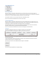
ExcelCalculationSettings:CurrentCalculationMode
You can use this form to view and change Excel’s current calculation status and settings. By default the current Excel calculation mode applies to all the open workbooks. Also all the open workbooks are recalculated, not just one Excel’s default calculation mode is at the Excel session level. This means that Excel will use the same calculation mode for all open workbooks, regardless of the calculation mode that was saved with an individual workbook. Whenever Excel calculates the default behavior is to calculate all the open workbooks, rather than just the active workbook Automatic
Formulas are recalculated automatically whenever anything changes so that the workbook(s) are always calculated. AutomaticexceptTables
Similar to automatic except that Excel Tables are not automatically calculated. This can be useful with large workbooks because Excel Tables cause multiple calculations of the workbook. Manual
The status bar will also show “Calculate” if there are circular references or more than 655536 dependencies in Excel 97‐2003 or ForceFullCalculation has been turned on. Formulas are only recalculated when the user requests it by pressing F9 or the FastExcel recalculate button. When the workbook is not completely calculated the status bar shows “calculate”. Recalculatebeforesave.
If in Manual mode checking this option will cause Excel to recalculate uncalculated formulas in the workbook each time it is saved. FastExcelActiveWorkbookMode
Open multiple workbooks but only calculate the active one. Set different calculation modes for each open workbook with Set Book Modes. FastExcel V3 User Guide
FastExcel V3: Controlling Calculation  43
Whilst this option is active you cannot copy and paste between workbooks. Excel normally calculates all the workbooks you have open at each calculation. This can cause inconvenience and slow calculation when you have multiple workbooks open. FastExcel allows you to set Active Workbook Mode so that Excel will only calculate the active workbook. When you set Active Workbook Mode the default is that each open workbook is in Manual calculation mode, so that you have to press F9 to calculate the Active Workbook. For more complicated situations FastExcel allows you to set different calculation modes for each workbook. For example suppose one workbook is set to Automatic and another to Manual: 
If the Automatic workbook is active then it will be automatically calculated at any change to the workbook, but the inactive manual workbook would not be calculated. 
If the Manual workbook is active then it will only be calculated when you press F9, and the inactive Automatic workbook will not be calculated. You can set the calculation mode for each of the open workbooks (and the default mode) using the Set Book Modes button. This book calculation mode is saved with each workbook. If you use active workbook mode with a workbook in Automatic mode then it will be recalculated whenever you make it active. Once you set this option it will still be active the next time you open Excel. Whilst this option is active you cannot copy and paste between workbooks. You can use Active Workbook Mode for the workbooks at the same time as Mixed Mode for the worksheets, but Mixed Mode is not dependent on Active Workbook Mode. FastExcel V3 User Guide
FastExcel V3: Controlling Calculation  44
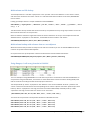
ExcelCalculationSettings:SetBookModes
DefaultActiveWorkbookCalculationMode
The Default Workbook calculation Mode only applies when you have selected Active Workbook Mode. You can change the FastExcel default workbook calculation mode whenever you want. The FastExcel default will apply to all workbooks in Active Workbook Mode until changed, and will be recalled when you next open Excel. The default workbook calculation mode is used in active workbook mode to calculate a workbook with no assigned workbook calculation mode, or one assigned a mode of default. The initial default mode is Manual. SetBookCalculationModes
The workbook calculation mode for each workbook can be: 
Manual 
Automatic 
Semi‐automatic (Automatic except Tables) 
Default: The workbook will use the current default workbook calculation mode. To change the workbook calculation mode for one or more workbooks, select the workbooks and press one of the calculation mode buttons. FastExcel V3 User Guide
FastExcel V3: Controlling Calculation  45
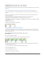
ExcelCalculationSettings:InitialCalculationMode
You can use these settings to control which calculation mode Excel will use when opened. By default the first workbook opened sets the mode until it is changed by the user Force Excel to open in Manual mode to prevent your workbook being accidentally recalculated when you open it By default Excel sets the initial calculation mode from the first workbook opened, and does not automatically change it when another workbook with a different setting is opened. FastExcel allows you to control the mode to be used when Excel first opens. This initial mode can be: 
First Workbook (Excel default) 
Manual 
Manual with recalculate before save 
Automatic 
Automatic except tables Limitation: When you use FastExcel initial calculation mode the empty workbook (Book1) that Excel creates when it is started will prompt you to save it when you close Excel. ExcelCalculationSettings:Iteration
These settings control how Excel handles circular references. Iteration
When checked Excel will attempt to resolve formulas that are linked by circular references by repeatedly calculating them. MaximumiterationsandMaximumchange
Excel will stop the repeated calculation of the circular references as soon as either the maximum number of iterations has been reached or the maximum change in the values of all of the formulas is less that the specified maximum change. FastExcel V3 User Guide
FastExcel V3: Controlling Calculation  46
Multi‐threadedcalculationSettings
EnableMTC
When Checked Excel (2007 and later) will split the calculation process over multiple threads. This will improve calculation speed on many problems, particularly with large workbooks and multiple recalculations. UseallProcessors/ManuallyAssignthreads
You can control the maximum number of threads to be used by Multi‐Threaded calculation FastExcel V3 User Guide
FastExcel V3: Controlling Calculation  47
ExcelCalculationSettings:CalculationButtons
The calculation timer for these buttons is controlled by your FastExcel settings The Excel Calculation Settings Tab also contains buttons to request various types of calculation. FastExcel will show the time taken by the calculation if the calculation timer for buttons is switched on. Using FastExcel defaults Excel will calculate all enabled worksheets in all open workbooks, and will calculate all MixMode sheets with a Full calculate, and selected MixMode sheets with a Sheet calculate. CalcFullRebuild(Shift‐Ctrl‐Alt‐F9)
By default MixMode sheets are calculated if Mixed Mode Full Calculate is on Calculate Full Rebuild rebuilds the dependency trees and then fully calculates all formulas in all open workbooks. This option is only available from Excel 2002 onwards. CalcFull(Ctrl‐Alt‐F9)
By default MixMode sheets are calculated if Mixed Mode Full Calculate is on Calculate Full fully calculates all formulas in all open workbooks. Recalc(F9)
By default MixMode sheets are calculated if calculation mode is manual and Mixed Mode Manual is on Recalculate recalculates all formulas that have been changed or are volatile, or are dependent on a cell that has been changed or recalculated. RecalcSheet(Shift‐F9)
By default MixMode sheets are calculated if Mixed mode selected sheets is on Recalculate Sheet recalculates all formulas on each selected sheet that have been changed or are volatile or are dependent on a cell on the selected sheet that has been changed or recalculated. FastExcel V3 User Guide
FastExcel V3: Controlling Calculation  48
FullcalcSheet(Alt‐Shift‐F9)
By default MixMode sheets are calculated if Mixed mode selected sheets is on Full Calculate Sheet calculates all formulas on each selected sheet. CalcRange(Alt‐F9)
Calculates even on MixMode sheets Range Calculate calculates the selected range. DirtyRange
Flags the selected cells as uncalculated. This option is only available in Excel 2002 or later. In automatic mode this will trigger a recalculation. MixModeRecalc(Ctrl‐Shift‐F9)
Recalculates both MixMode and ordinary sheets. MixMode Recalc is similar to Recalc (F9), except that the recalculation also includes all Mixed Mode sheets. FastExcel V3 User Guide
FastExcel V3: Controlling Calculation  49
WorkbookCalculationSettings
WorkbookCalculationSettings:MixedMode
OptionsforcalculatingMixModeWorksheets
Make some sheets calculate automatically and others only when you request calculation FastExcel allows you to mix calculation modes for different worksheets within a workbook. The default settings are designed to allow you to use either automatic or manual calculation for normal sheets, but only calculate specified MixMode sheets when you need to. You can use mixed mode at the same time as Active Workbook mode. 
You can choose which worksheets to designate as MixMode sheets. 
MixMode worksheet settings are stored with the workbook and persist between Excel sessions. 
You can use default settings or customize the settings. 
MixMode worksheets can be combined with the new calculate active workbook only mode and the ability to set calculation mode by workbook. MixedModedefaultsettings
If Active Workbook Mode is ON then only the active workbook is calculated: if Active Workbook Mode is OFF then all open workbooks are calculated When you use FastExcel’s default MixMode settings Excel calculates as follows: 
In automatic calculation mode MixMode sheets are not recalculated automatically. 
F9 or the Calculate button will not recalculate MixMode worksheets. 
Ctrl/Shift/F9 or the Calculate MixMode Sheets button will recalculate the workbook(s) including MixMode sheets. 
Shift/F9 or the Calculate Sheet(s) button will calculate all the selected sheets including any selected MixMode sheets. If in automatic mode the workbook(s) will then also be recalculated. 
Ctrl/Alt/F9 or the Full Calculate Button will calculate all formulas on all sheets in all workbooks, including MixMode sheets. ControllingMixedModeSettings
Mixed Mode calculation of MixMode sheets occurs for all open workbooks unless you have selected Active Workbook Mode. FastExcel V3 User Guide
FastExcel V3: Controlling Calculation  50
You can control MixMode sheets will be calculated using these options: 
Full Calculation: when this option is checked all formulas including those on MixMode sheets in the active workbook will be calculated when you press Ctrl‐Alt‐F9 or the FastExcel Full Calculate button. The default is checked. 
Manual Calculation: when this option is checked pressing F9 or FastExcel’s Recalculate button will recalculate formulas that are flagged as uncalculated, including those on MixMode sheets in the active workbook. The default is not checked. 
Selected Sheet(s) Calculation: when this option is checked pressing Shift‐F9 or FastExcel’s Calculate Sheets button will recalculate formulas that are flagged as uncalculated on all selected sheets, MixMode or enabled. The default is checked. 
Automatic Calculation: this option is permanently disabled: Excel’s automatic calculations do not recalculate MixMode sheets (except when you enable them of course). You can select which sheets will be MixMode sheets using the Select MixMode Sheets button. Whenaworkbookisopened
If Excel is in automatic mode all MixMode sheets are recalculated. If Excel is in manual mode any MixMode sheets are not recalculated unless the “Calculate MixMode sheets on open” option (Workbook Calculation Settings tab) was selected when the workbook was saved. UsingRangeCalculateinMixedMode
Range calculate or Alt‐F9 always calculates the selected range even on a MixMode sheet. FastExcel V3 User Guide
FastExcel V3: Controlling Calculation  51
WorkbookCalculationsettings:ChoosingtheMixModeSheets
You can choose which sheets to process in Mixed mode using the Select Mixmode Sheets button on the Active Workbook Calculation settings tab. FastExcel stores these settings for each worksheet in the workbook, and restores the last saved settings when the workbook is opened. Use this command to select the sheets you want to be handled as MixMode sheets. These sheets will be calculated according to the options set for Mixed Mode calculations. You can also use this tool to explore the possible effect of combining sheets. In cases where there is a significant workbook calculation overhead you may be able to simulate the effect of combining the sheets causing the bottleneck by setting suspect worksheets to MixMode and monitoring the effect on workbook recalculation time. NOTE: When using FastExcel Version 3 these settings are saved when you save a workbook and restored when you open a workbook. These settings use Excel’s Worksheet Enable Calculation property. This behavior is different to the standard Excel behavior. FastExcel V3 User Guide
FastExcel V3: Controlling Calculation  52
WorkbookCalculationSettings:WorkbookOptions
RestoreWorkbookCalculationModeafteropen
This option only functions when: ‐the workbook has been saved ‐and the workbook is subsequently opened. When Restore calculation mode after open is checked FastExcel will automatically reset the calculation mode after the workbook has been opened to the workbook calculation mode. You can set the workbook calculation mode using Set Book Modes, or let it default to the default workbook calculation mode, which you can also set in Set Book Modes.
Note that using this option does NOT prevent Excel calculating a workbook when it is opened and Excel is in Automatic mode. Use “Restore calculation mode after open” instead of Active Workbook Mode if you want to force Excel into the calculation mode of this workbook whenever it is opened, but do not want to switch calculation mode whenever a workbook is activated. ForceFullCalculation
This option is only available in Excel 2007 or later. If checked every calculation on this workbook will be a full calculation rather than a recalculation, and the time taken to rebuild the dependency trees will not be needed at workbook open time or when the workbook is edited. Switch on Force Full Calculation if adding a row at the top of a worksheet is very slow and Full Calculate time is close to Recalculate time. CalculateMixModesheetsonopen
Only works if FastExcel was active when the workbook was saved Calculate all worksheets including MixMode when the workbook is opened in manual mode. In Automatic mode MixMode sheets are always recalculated on open, so you cannot select this option when calculation mode is automatic. UpdateRemoteReferences
If TRUE automatically update any remote references (DDE Links to other programs) whenever Excel recalculates. FastExcel V3 User Guide
FastExcel V3: Controlling Calculation  53
SaveExternalLinkValues
If TRUE Excel will save values for the links to external workbooks. I recommend keeping this option as TRUE PrecisionasDisplayed
Checking this box will force Excel to calculate to the number of decimal places that appear as a result of your formatting, and will permanently change any numbers stored in cells. You need to be sure you have thought through the full implications of this before using it. Precision as Displayed slows down calculation. 1904DateSystem
If TRUE changes the starting date from which all dates are calculated from January 1 1900 to January 2 1904. AcceptLabelsinFormulas
This allows Excel to use natural language labels in formulas. Because there are circumstances when this will give you unexpected or ambiguous results, I recommend you do NOT use this feature. FastExcel V3 User Guide
FastExcel V3: Controlling Calculation  54
FastExcelSettings
CalculationTimersforbuttonsandkeys
You can control the FastExcel calculation time display separately for the calculate buttons and the calculate keys. The calculate buttons are the buttons on the FastExcel toolbar and on the Excel Calculation Control Group of the FastExcel V3 Tab form. When checked you will see a message box after the calculation showing the time taken by the calculation. RangeCalculateSettings
RangeCalcincludingorexcludingDependents
In Excel 2007 and later there are 2 different Range calculate methods. One includes within‐range dependency calculations and the other ignores within‐range dependencies and calculates row by row strictly left‐to‐right and top‐to‐bottom. Range Calculate always ignores dependencies outside the selected range, although the selected range will be expanded to include all the cells in multi‐cell array formulas. SetNumberofRangeCalcTrials
Because RangeCalc timing can be sensitive to Windows multi‐tasking it is better to allow a number of trials. The Median (middle‐most) calculation time will automatically be used, thus discarding incorrectly high and low values. You can set the number of trials: the default number is 3. IncludeScreenRefreshTime
If checked timings for Range Calculate will include the time used by Excel to refresh the visible window. FastExcel V3 User Guide
FastExcel V3: Controlling Calculation  55
LookupMemorySettings
FastExcel SpeedTools defaults to saving the Lookup Memory data in the workbook, and restores the Lookup Memory when the workbook opens. If you do not want to store the Lookup Memory you can switch of the save process by un‐checking the Save Memory with Workbook box. If you want to force storing the Lookup Memory data externally to the workbook check the Always Store Externally box. You can use this option in conjunction with the retrieve memory button to transfer lookup memory between workbooks. Clear Memory clears the currently active Lookup Memory, but does not delete it from an already saved workbook. Count Lookup Memory shows you the number of lookup memory values by type. Retrieve Memory tries to get Lookup Memory from the workbook, and if there is no Lookup Memory stored within the workbook will then look for external Lookup Memory files. FastExcel V3 User Guide
FastExcel V3: Controlling Calculation  56
FastExcelV3LicensingSettings
Show License Status shows you the status of your licenses for all FastExcel V3 products. Add New License asks which product you want to add a license for: FastExcel V3 User Guide
FastExcel V3: Controlling Calculation  57
And then prompts for the License Activation key.
FastExcel V3 User Guide
FastExcel V3: Controlling Calculation  58
CalculationTimingCommands
There are seven FastExcel V3 timing commands. ThesevenCalculationbuttons
These seven calculation buttons calculate the selected items and optionally show you the elapsed time taken by the calculation. Use FastExcel Calculation Control‐>FastExcel Settings to choose between the 2 available Range Calculate methods (with or without dependencies internal to the selected range) and the number of Range Calculate trials (default 3). Range Calculate then shows the median time of all the trials. The currently selected cells, using Range Calculate. Alt‐F9 If more than one Area is selected; each Area is calculated left‐to‐right and top‐to‐bottom, in the sequence that the areas were selected. If more than one worksheet is selected then only the selected range on the active worksheet is calculated. If one or more of the selected cells is part of a multi‐cell array formula then all the cells in the array formula will be included in the calculation.
If Calculation is set to Automatic both the time taken to calculate the range in Manual mode and the workbook recalculation time are shown. Sheet Calculate re calculates the selected Sheets assuming that all precedent worksheets and linked workbooks have been correctly calculated. Full Calculate Sheet calculates every formula on the selected Sheets assuming that all precedent worksheets and linked workbooks have been correctly calculated. FastExcel V3 User Guide
The currently selected sheet(s), using Sheet Recalculate. Shift‐
F9. If more than one worksheet is selected all the selected worksheets are recalculated. If Calculation is set to Automatic both the time taken to recalculate the sheet(s) in Manual mode and the subsequent workbook recalculation time are shown. If MixMode sheets are selected by default they will be calculated The currently selected sheet(s), using Sheet Full Calculate. Alt‐Shift‐F9. If more than one worksheet is selected all the selected worksheets are recalculated. If Calculation is set to Automatic both the Calculation Timing Commands  59
Recalculation is the default Excel calculation process. Only changed cells and formulas dependent on changed cells are calculated Full calculation calculates all formulas in all open workbooks time taken to recalculate the sheet(s) in Manual mode and the subsequent workbook recalculation time are shown. If MixMode sheets are selected by default they will be calculated All enabled sheets in open workbooks. Recalculate. F9. MixMode sheets are not calculated unless Manual Calculation has been checked in MixMode options. Calculate all open workbooks. Full Calculation. Ctrl‐Alt‐F9 Recalc MixMode Sheets recalculates all sheets including MixMode sheets. FastExcel V3 User Guide
Recalculate MixMode Sheets: All enabled sheets and any MixMode sheets in all open workbooks are recalculated. Ctrl‐Shift‐F9. Select, run and time a macro. To control the display of the calculation time see FastExcel Calculation Calculation Timing Commands  60
Control ‐> FastExcel Settings. There are keyboard shortcuts for these calculation commands. The GoTo command is context sensitive to the active sheet. If the active sheet is: 
The output sheet from Profile Formulas and Functions. GoTo will attempt to go to and select the Formula that has been selected on the Profile. If no formula has been selected then the first formula will be used. 
The output sheet from Profile Worksheet Formulas. GoTo will attempt to go to and select the Area that has been selected on the Profile. If no formula has been selected then the first Area will be used. 
The output sheet from Map Formats or Map Styles. If you select a cell that contains the number of Styles or Number Formats on a worksheet then GoTo will attempt to select ALL the cells on that worksheet that have that Number Format or Style. 
Any other sheet. GoTo will ask if you want to go to cells with the same Style or Number Format or direct precedents. Go Back reverses the last GoTo. FastExcel V3 User Guide
Calculation Timing Commands  61
GettingConsistentResultsfromFastExcelV3Timing
Sometimes you will find that your FastExcel timing results are not repeatable, even though FastExcel measures elapsed time using a high‐resolution timer with microsecond accuracy. PowerSavingandDualCoreIntelandAMDprocessors:
Power saving features, particularly on dual‐core processors, may dynamically vary the speed of your processor. This can create problems for consistent timings using the high‐resolution timer. If timing consistency is important try switching off the power‐saving features of your processor. Excelminimizesthenumberofcalculations:
When Excel calculates it remembers: The second calculate is often much faster than the first 
Which cells have been calculated. 
The optimum calculation path used for the final answer. So the next time Excel calculates it can save time by: 

Only calculating the cells that have changed (or depend on cells that have changed) Re‐using the last calculation path WhyFastExcelTimingresultsmayvaryfromruntorun:
Both Excel and Windows cache information to speed up subsequent operations Windows is a multitasking system so Excel does not get the whole system to itself Both Excel and Windows try to optimize performance by storing recent information in memory. This includes the calculation path used by the most recent calculation. So Excel’s second calculate is often significantly faster than the first. Excel also saves some of this information, including the most recent calculation path, with the workbook. Excel’s background calculation process can easily be interrupted Windows is a multitasking, paged virtual memory operating system so other system tasks are always running at the same time as Excel. Try and make sure there are no other user tasks active whilst you are using FastExcel. Excel’s background calculation process can be interrupted if you press any key or click the mouse whilst FastExcel is active. This may give you inaccurate timings. FastExcel V3 User Guide
Calculation Timing Commands  62
ProfilingCommands
TheProfilingCommands
The five profiling commands are: Drill‐down Wizard: This guides you to drill down to find the calculation bottlenecks from workbook to worksheets to worksheet areas to individual formulas and functions. Profile Workbook: which analyzes the calculation times and memory usage of your workbook. Profile Worksheet Areas: This analyzes formula calculation times for the columns, rows and blocks of formulas in one or more of your worksheets. Profile Worksheet Formulas and Functions: This analyzes the calculation times for unique formulas on a worksheet and identifies the functions used that are volatile or single‐threaded. Map Worksheet Cross‐References: This analyzes the cross‐references between worksheets and optionally re‐sequences the worksheets to minimize forward cross‐references. Note: The Trial version of FastExcel Profiler will only profile a single worksheet using the Drill‐down Wizard. The Profile Workbook, Profile Worksheet and Profile Formulas commands are not available when using the trial version of FastExcel Profiler. You can get Contextual Help on the output from the profiling commands either by right‐clicking a selected cell on the output sheet or by selecting a cell and pressing the FastExcel Contextual Help button. Potential bottlenecks are highlighted in orange. The sensitivity of the orange highlighting can be controlled by setting FastExcel’s Orange Tolerance (default 0.2) on the FastExcel Settings page: Cell Highlight (Orange) sensitivity. The profiling commands help you to document calculation options, and generate timing statistics and memory usage details. The profiling commands generate result worksheets into a separate workbook, using sheets called: 
FastXLBookn: The workbook profile results 
FastXLSheetn: the worksheet profile results 
FastXLFuncsn: the worksheet formulas and functions profile results FastExcel V3 User Guide
Profiling Commands  63

FastXLPrecsn: the worksheet cross‐reference map results Multiple profiles of a given type are given an incremental number suffix. FastExcel V3 User Guide
Profiling Commands  64
UsingtheDrill‐DownProfilingWizard
If you would like to get some immediate results on your workbooks without delving into lots of details you can simply use the Drill‐down Wizard to find the Calculation Bottlenecks in an easy step‐by‐step way. They key to the Drill‐Down Wizard is that it can recognize the output results sheets from Profile Workbook and Profile Worksheet (FastXLBook and FastXLSheet) and use them to drill down into the worst‐performing sheet, area and formulas. If the active sheet is not a result sheet from a previous Profile the Drill‐down Wizard starts by Profiling the Workbook. If the active sheet IS a result sheet from a previous profile the Drill‐down Wizard can either drill into the worst thing found at the top of the list, or will work on a selected result. So it’s easy to use the Drill‐down wizard in a step‐by‐step sequence: 


Profile the Active Workbook to find the worst performing worksheets. With the results sheet (FastXLBook1) from the Profile Workbook active to identify the worst worksheet, Profile that worksheet to find the worst Area. With the results sheet (FastXLSheet1) from the previous step active to identify the worst area, Profile that area to find the worst‐performing formulas and functions. You can then repeat the process for a different worksheet by selecting the result row for another sheet on the FastXLBook1 sheet and starting the Drill‐down wizard again. Or you can repeat the process for a different area by selecting an area result row on a FastXLSheet worksheet and starting the drill‐down wizard from there. Note: The Trial version of FastExcel Profiler will only profile a single worksheet, a single Worksheet Area and a single block of formulas using the Drill‐down Wizard. The individual Profile Workbook, Profile Worksheet and Profile Formulas commands are not available when using the trial version of FastExcel Profiler. FastExcel V3 User Guide
Profiling Commands  65
TheProfilingHeader
All five profiling commands document the profiled workbook by showing a common set of header tables: ThePhysicalEnvironmentTable
Cells with red dots contain on‐sheet Notes: hover your cursor to make them pop‐
up. The Physical Environment Table shows information about the system. Orange if Memory Used>1MB and (Memory Used +64)>RAM (MB) 
RAM (K): Physical Memory Used and installed in K bytes. You should have at least enough physical memory installed for Windows, Excel and all the open workbooks. See Bottlenecks. Orange if Used/Available > 3.75 * Orange Tolerance 
Swap File (K): Swap File used and Swap file available in K bytes. If your system is using a large amount of your existing swap file either close as many programs as possible FastExcel V3 User Guide
Profiling Commands  66
Orange if Used/Available> 3.75*Orange Tolerance or increase the size of your swap file. 
Excel Memory (K): Excel Memory Used and available. Total Memory Used by all open Excel workbooks for data, formulas etc. (excludes Memory Used by the Excel program itself), and the maximum Excel workbook memory available for formulas etc. K Bytes. Excel97 and 2000 have a limit of about 80MB of memory for formulas and pivot caches. Excel2002 has a limit of about 160MB and Excel 2003 has a limit of about 1024MB. The limit for Excel 2007 and later 32‐bit Excel versions is about 2048MB, and for 64‐bit Excel versions 192GB under Win 7 and 512GB under Win 8. Note that there are additional limits (Charts etc.) that may cause Excel to run out of memory before all available workbook memory is used. 
FileSize (K): The size on disk of the workbook in Kilobytes. 
Windows: The version of Windows in use when this profile was created. 
MHZ x Cores: For Windows NT, 2000 and XP, the processor speed in MHZ, and the number of processor cores in the system. 
XLVersion: the Excel version number and bitness used for this profile: 
FastExcel V3 User Guide

Excel 97 is Version 8 
Excel 2000 is Version 9 
Excel 2002 is Version 10 
Excel 2003 is Version 11 
Excel 2007 is Version 12 
Excel 2010 is Version 14 
Excel 2013 is Version 15 XL Calculation Engine: The version number of the calculation engine that was used for this profile. If not Excel 2000 or a later version, N/A. Profiling Commands  67
TheWorkbookSettingsTable.
The Workbook Settings Table shows basic information on the profiled workbook: 
If Shared and Keep Change History are both true they are colored orange. 


Avoid saving in Dual Format 





Colored orange if true 



FastExcel V3 User Guide
The name and path of the profiled workbook and the date and time that the profile was created. (Not shown in the above picture) Shared: True if the Workbook is open for Sharing. If Shared and Keep Change History are both true the Workbook size can grow considerably. Changes: Keep Change History Tracking: True if enabled, otherwise False. If Shared and Keep Change History are both true the Workbook size can grow considerably. Saved: False if the workbook has been changed in any way since the last save. Format: the format of the saved workbook: Dual Format (Orange) doubles the file size. Fixed: Fixed Decimal: If True numbers will be treated as having an implied decimal point, in the position given by Places below. Places: The position of the implied decimal point, if Fixed Decimal is true. Backup: True if a backup copy of the workbook will be created when you save. Styles: The number of Styles in the workbook. If this number is large you may want to use Clean Workbook to map where the styles are being used, and to remove unused styles. Protection: The following three items show the protection status of the Workbook structure and windows, and whether the book is password protected. Structure: True if the structure of the workbook is protected. If protected with a password then opening the workbook will be slow. Worksheets: True if the worksheets in the workbook are protected. Password: True if the workbook is Password protected. Views: The number of Views in the workbook. Profiling Commands  68
TheEnvironmentCountsTable

XLB/Qat (K): The size of the XLB and QAT files in K Bytes. The XLB file stores toolbar customizations. The QAT file stores ribbon customizations. When they get large they may become corrupted and cause memory problems. The XLB file is located in %AppData%\Microsoft\Excel and the QAT file is located in %LocalAppData%\Microsoft\Office\ 
COM Addins: The number of COM addins currently loaded 
Temp: Count of the temporary files in your Windows temporary directory and subfolders. A large number of Temp files may make your workbook slow to open or cause Excel to crash. The Clean Workbook command can delete all temporary files that are not currently being used. Colored orange if >100 Note: a very large number of temp files may cause FastExcel to hang with the status bar showing “Checking Temp Files”. If this occurs close Excel, reboot your PC and then delete all files in your temp folder. You can locate your temp folder using StartRun, entering %temp% in the run box and pressing enter. Colored orange if >15 
VBE: Total Number of Windows in use by the VBE IDE. Includes hidden windows. A large number of open VBE Windows consumes resources and may cause memory problems. (If blank in Excel 2002 or later check "Allow access to Visual Basic Project" in Tools, Macros, and Security). The Clean Workbook command can close all unnecessary VBE Windows. 
Addins: The number of Excel Add‐Ins currently loaded by Excel’s Addin Manager. This excludes any addins that have been loaded using File Open or the Decision Models Addin Loader. FastExcel V3 User Guide
Profiling Commands  69
TheCalculationSettingsTables.
See FastExcel Calculation Options for a detailed description of these options and how to set them You can use the FastExcel Calculation Options button to change these calculation settings. TheExcelCalculationSettingsTable
By default Excel Calculation Settings apply to all currently open workbooks. FastExcel Active Workbook mode allows you to control Calculation for the active workbook instead of all open workbooks. FastExcel Mixed Mode allows you to select sheets as MixMode sheets and control whether they will be calculated in Automatic, Manual or Sheet calculate. 






FastExcel V3 User Guide
Workbook Mode: All or Active Book. The Excel default is to calculate all the open workbooks. With FastExcel you can restrict calculation to the active workbook only (and each workbook can have a different calculation mode, see Mixed Mode processing). Current Mode: Automatic, Manual or Semiautomatic. This mode applies to all the open workbooks or just to the active book. The Excel default is to apply this mode to all the worksheets in a book. With FastExcel’s Mixed Mode you can control which worksheets are calculated in Automatic or Manual or Sheet Calculate mode. Before Save: If True Excel will recalculate before each save. Any worksheets that are NOT enabled for calculation will not be calculated. Initial Mode: Controls how Excel sets the calculation mode when started. First Workbook (Excel Default): Calculation mode is set from the first workbook opened. Automatic: Calculation mode will be set to automatic. Manual: Calculation mode will be set to Manual. Semi‐Automatic: Calculation mode will be set to Automatic except Tables. Iteration: If TRUE Excel will attempt to resolve circular references by iteration. Max Iters: the maximum number of iterations used to resolve circular references. MaxChange: Iteration will stop when no cell changes by more than MaxChange Profiling Commands  70






FastExcel V3 User Guide
Multi‐Threaded Calc: Calculation using multiple cores and threads On: True/False/ #N/A Shows if Multi‐Threaded Calculation (MTC) is on, off or not available Mode: Automatic – Excel assigns a calculation thread to each available core. Manual – the user has assigned a specific number of threads. Threads: The number of threads assigned to the calculation. Force Full Calc: Shows if this workbook will use Excel’s smart recalc or always calculate every formula in the workbook at each calculation. Full/Recalc: Full: every formula in all open workbooks will be calculated at each calculation Recalc: only changed formulas and formulas dependent on changed values/volatile cells will be recalculated XL 64K Limit: in Excel versions prior to Excel 2007 Excel switched to force‐full calculation when dependencies exceeded 64K. Colored orange if this limit has been reached Profiling Commands  71
TheWorkbookCalculationSettingsTable
These settings can be different for each open workbook You can use Mixed Mode so that some worksheets always calculate and others calculate only when you want. FastExcel V3 User Guide

Mixed Mode allows you to choose when any MixMode sheets will be calculated. 
Full: If True any MixMode worksheets will be recalculated at each full recalculation (Ctrl/Alt/F9). 
Manual: If True any MixMode worksheets will be recalculated at each Manual calculation (F9). 
Selected Sheets: If true then any MixMode sheets that are selected will be calculated when Sheet Calculate or Shift‐F9 is pressed. 
Restore After Open: If True then FastExcel will automatically reset the calculation mode after the workbook has been opened to the mode that was active when the workbook was saved, or in Active Workbook Mode to the mode stored in the workbook 
MixMode on Open: If Excel is in Automatic mode then all the MixMode sheets in the workbook being opened will be recalculated. If Excel is in Manual mode any MixMode sheets will not be calculated when the workbook is opened unless this option is True. 
Update Remote Refs: If TRUE automatically update any remote references (DDE Links to other programs) whenever Excel recalculates. 
Precision as Displayed: If TRUE uses the displayed value of all cells rather than their real value as input to subsequent formulas. Be careful because this also permanently changes the values of numeric constants. 
1904 Date System: if True changes the starting date from which all dates are calculated from January 1 1900 to January 2 1904. 
Save External Link Values: If TRUE Excel saves values for links to external workbooks. 
Book Calc Engine: The version number of the calculation engine that last calculated the workbook (if not Excel 2000 or a later version then N/A). Colored orange if less than the Application calculation version Profiling Commands  72
ProfileWorkbook:ProfiletheactiveWorkbookandallitsWorksheets.
Profile Workbook: Profile the active workbook and all its worksheets. This command is not available when using the trial version of FastExcel Profiler. Because Excel calculates all open workbooks rather than just the active workbook you can get misleading calculation times if you have multiple workbooks open during Profile Workbook. ChooseProfileWorkbookOptions
 Because Profile Workbook can take a long time to execute these options allow you to include or omit various profiling options:  Profile all the worksheets: if switched off the individual worksheets will not be profiled.  Profile Sheet Memory: this can be a very time consuming option and is switched off by default.  Profile Multi‐Threaded Calculation: If checked each worksheet will be calculated once using multi‐threaded calculation and once without so that the multi‐threaded calculation efficiency of each sheet can be determined.  Profile Worksheet Volatility: If checked each worksheet will be calculated once using smart Recalc and once using Full Calculation so that the worksheet volatility can be determined.  Profile Worksheet Sparseness: If checked the number of cells containing constants will be counted and the sparseness % of the real used range will be calculated.  Profile the workbook itself: If switched off the workbook itself will not be profiled.  Profile Multi‐threaded Calculation: if checked the workbook will be calculated once using MTC and once without so that the multi‐threaded calculation efficiency of the workbook can be determined.  Profile Workbook Volatility: If checked the workbook will be calculated once using smart Recalc and once using Full Calculation so that the workbook volatility can be determined.  Events during Calculation: Profile Workbook will by default attempt to prevent VBA events from occurring during the timed calculations. If your workbook contains event‐handling VBA code you should consider whether to include or exclude it when running Profile Workbook.  Set Warning Tolerance: a larger tolerance number reduces the number of orange warnings produced. FastExcel V3 User Guide
Profiling Commands  73
Profile Workbook produces information in several tables: 
Excel and Workbook environment information and calculation options. 
Worksheet cell counts, calculation times and Memory Used 
Workbook summary Potential bottlenecks are highlighted in orange. The sensitivity of the orange highlighting can be controlled by setting FastExcel’s Orange Tolerance (default 0.2). TheWorksheetProfilesTable.
The Worksheet Profiles Table shows the cell counts, calculation times and Memory Used for each worksheet. The table is only produced if the Profile All the Worksheets option is checked in the Profile Workbook Options. The worksheets are sorted in descending sheet calculation time. FastExcel V3 User Guide
Profiling Commands  74
TheWorksheetProfilesTable:CellCountsColumns
Cell counts show you the key size statistics for each worksheet. The Cell Counts columns show counts of the number of cells for: 
Used: The Used Range: The rectangular table of cells that Excel considers used: Excel considers cells with formatting, data or formulas used. The Used Range is not automatically reset when cells are deleted or cleared. You can clean up the Used Range with Clean Workbook.Constants: the number of constants on this worksheet. 
CondFmt: the total number of conditional formats on this worksheet. Colored orange if the average number of conditional formats per conditionally formatted cells is > 3. 
Formula: the number of formulas on this worksheet. 
CondFormat Enabled: shows you if conditional format calculation is enabled for this worksheet. FastExcel V3 User Guide
Profiling Commands  75
TheWorksheetProfilesTable:CalculationTimes.
In the actual FastExcel output these columns are adjacent to the cell counts columns rather than as shown above. Calc Time (Millisec); the elapsed calculation times in milliseconds. Use this table to identify the sheets that use the most calculation time, any sheets with significant volatility or MTC inefficiency and the sheets that have the most expensive formulas. Colored orange if >orange tolerance * total sheet calc time and > (1+orange tolerance)*minimum sheet overhead and > orange tolerance * 500 FastExcel V3 User Guide
Range: Time in milliseconds for a Range.Calculate of the real used range in the worksheet, not using multi‐threaded calculation, minus the time taken to range calculate an empty worksheet (empty sheet overhead).This calculation ignores dependencies in Excel 97 and 2000. Recalc: The time taken to recalculate the sheet after the workbook has been calculated, minus the time taken to recalculate an empty sheet (empty sheet overhead). Multi‐threaded calculation is used if enabled. For most workbooks this will give a minimum worksheet calculation time because only the minimum set of formulas (mostly volatile formulas and their dependents) will be calculated. Full Calc: The time taken to calculate all the formulae on the sheet, minus the time taken to fullcalc an empty sheet (empty sheet overhead). Multi‐threaded calculation is used if enabled. Colored orange if > (1+ orange tolerance) *average sheet full calc Profiling Commands  76
Colored orange if >(1+ orange tolerance) * average and > orange tolerance * 500 FastExcel V3 User Guide
time and >orange tolerance *500 Sheet Volatile %: The Ratio of Sheet Recalc time to Sheet Full Calc time.
Measures how many of the formulae on the sheet are volatile. Colored orange if >orange tolerance * .125 Sheet MTC Factor: A measure of the efficiency of multi‐threaded calculation at sheet level. The ratio of Range calculation (single‐
threaded) time to Full Calculation (multi‐threaded) time. Other: The three times shown in the Other row are the times taken to calculate an empty worksheet. These times are used as standard calculation overheads and are subtracted from the sheet calculation times. Sheet % Volatile: The ratio of Recalc time to Full Calc time, excluding standard calculation overhead. When you have a high workbook volatility % you can use the sheet % volatile to determine which sheets are causing the problem. Microseconds per Formula: calculated from the smaller of used range calc time and sheet calc time. A high value may indicate bottleneck formulas. Profiling Commands  77
WorksheetProfilesTable(2)
In the actual FastExcel output these columns are adjacent to the Calc Times columns rather than as shown above. Sheet Memory: the Memory Used by this worksheet. This includes Pivot Caches. Other: This is memory used by the workbook excluding memory used by the worksheets. Colored orange if > (1 + 3.75 * orange tolerance) *average memory per cell and used range memory > 50 * orange tolerance Unused Cells: Eliminate the waste by using FastExcel’s Workbook Cleaner Sheet bytes per Cell: Memory used per cell: calculated as. Worksheet memory / (count of constants and formulae) Measured in Bytes %Waste: The cells in the Used Range (formatted cells, constants, formulas, deleted/cleared cells) beyond the real Used Range (formulas and constants), as a percentage of the Used Range: Colored orange if > orange tolerance * 10000 cells. Significant waste can use additional memory and calculation time. %Sparse: Cells not containing formulas or constants, as a percentage of the used range. Colored Orange if > orange tolerance * 10000 cells. FastExcel V3 User Guide
Profiling Commands  78
WorksheetProfilesTable(3)
Page Breaks: True if DisplayPageBreaks is enabled for this sheet: can slow down macros significantly. On sheet notes are counted as shapes Shapes Count: Count of the number of shapes in the Drawing layer for this sheet. Includes hidden and zero‐height shapes. Use FastExcel’s Clean Workbook command to remove zero‐height shapes. Colored orange if any of the shapes are linked by formula (slows calculation and editing). HyperLinks Count: Count of the number of Hyperlinks on this sheet. The hyperlinks can be internal or external to the workbook. Large numbers of hyperlinks can be slow. Sheet Calc Mode: Shows the MixMode calculation mode for the worksheet. 
Book: the Sheet will be calculated whenever the Workbook calculates 
F: The Sheet will be calculated at every Full workbook calculation. 
M: the Sheet will be calculated at every Manual workbook re‐calculation. 
S: Shift‐F9/worksheet Calculate will calculate the worksheet when it is selected Either Book or any combination of F M and S is allowed. FastExcel V3 User Guide
Profiling Commands  79
TheWorkbookSummaryTable.
Volatility% and MTC are key measures of calculation efficiency The Workbook Summary table shows the cell counts, workbook calculation times, workbook volatility, workbook overhead, bytes per cell, and names count, for the profiled workbook. The workbook Summary table is only produced if the Analyze the Workbook option is checked in the FastExcel Settings. TheWorkbookSummaryTableCellCounts.
This shows totals of the counts for all the worksheets. TheWorkbookSummaryTableCalculationTimes.
Keeping Workbook Volatility low is often an excellent way to improve response time. Colored orange if > orange tolerance * 0.125 
Sheets Count: the total number of sheets in the workbook including Chart, Dialog, XLM Macro sheets as well as normal worksheets. 
Range: Total Time in milliseconds for Range.Calculate for the worksheets. The calculation is single‐threaded. This calculation ignores dependencies in Excel 97 and 2000. 
Recalc: milliseconds to recalculate (F9) the workbook immediately after a full calculation. 
FullCalc: milliseconds to fully calculate the workbook (Ctrl/Alt/F9). % Volatile is Recalculate Time as a percentage of full calculation time: a high value means one or more of: 



High proportions of the formulas are Volatile Evaluating the dependency trees takes a long time. The workbook is too complex for Excel to build a dependency tree (status bar always shows Calculate and there are no circular references). ForceFull calculation is true MTC Factor: A measure of the efficiency of multi‐threaded calculation at book level. The ratio of the sum of range calculation (single‐
threaded) times for each sheet to Full Calculation (multi‐threaded) time for the book. MicroSecs per Formula: Microseconds per formula based on full calculation time. FastExcel V3 User Guide
Profiling Commands  80
TheWorkbookSummaryTableMemory.
The actual FastExcel workbook summary output includes cell count column and calculation times. These columns are not shown in the above figure. 
Total Memory (K): Total Memory Used by this Work Book (K). If the Workbook is shared FastExcel cannot determine the memory of an individual worksheet. 
Bytes per Cell: Average of total memory used per cell. Calculated as: Total memory (Bytes) for all worksheets / (Total count of constants and formulae) In Bytes. 
%Waste: Cells in the UsedRange Outside the last Row and Column containing data or formulas, as a percentage of the cells in the usedrange. 
%Sparse: Sparseness of the UsedRange: Cells inside the used range, but not containing formulas or constants, as a percentage of the used range. 
Pivot Cache (K): Memory Used by Pivot Table Caches in this workbook in K bytes. 
XLLinks Count: The Number of Excel workbooks that are linked to by the profiled workbook. 
Names Count: count of the defined Names in the workbook. 
Open Time (Secs): The time taken to reopen the workbook. FastExcel V3 User Guide
Profiling Commands  81
ProfileWorksheetAreas:DetailsoftheFormulaareasontheSheets.
Profile Worksheet Areas: Shows the Profile Header block, and profiles each rectangular block of formulas and, optionally, each column and each block of rows on each of the selected worksheets. This command is not available when using the trial version of FastExcel Profiler. The Profile Worksheet Areas command shows you a form to allow you to choose between options. ChooseProfileWorksheetAreasOptions
You can choose to profile one or more of: 
The contiguous areas on the worksheet(s): either all or the selected areas. 
The Worksheet Columns within the areas: choose the number of groups of columns you want – larger number gives finer granularity but takes longer. 
The Worksheet Rows within the areas: choose the number of groups of rows you want – larger number gives finer granularity but takes longer. You can also choose to show counts of formulas and formula lengths – but this uses more time. The warning tolerance (Orange tolerance) controls the sensitivity of flagging the results as warnings. A larger number means more warnings. ProfileSelectedArea
After reviewing the output from a Profile Worksheet Areas you can select one or more of the problem areas on the worksheet that was profiled and use profile Selected Area to drill down into that area. FastExcel V3 User Guide
Profiling Commands  82
WorksheetAreasProfileTable
Use the tables to identify Bottleneck areas on the worksheet. There will be three Worksheet Areas Profile Tables for each of the selected Worksheets. All calculation times in these tables are single‐threaded calculation times. 


Cell counts of formulas, array cells and conditional formats. Calculation times for the area, column and the sheet. Total, average and maximum formula lengths. Each table is sorted in descending calculation time sequence. The first table profiles each separate contiguous rectangular area of formulas on the worksheet: The second table profiles the columns: the number of column groups should be no more than the number specified in the options. The column groups are sorted in descending calculation time sequence. The third table profiles the rows in the same way as the columns. FastExcel V3 User Guide
Profiling Commands  83
UsingtheFastExcelGoTocommandwiththeProfileWorksheetAreassheet
If you select one of the areas in the Profile Worksheet Areas output sheet and click the FastExcel GoTo button the area will be selected on its worksheet. If none of the areas are selected then the first area will be used. Subsequently clicking the FastExcel GoBackTo button will take you back to the profile worksheet areas result sheet. FastExcel V3 User Guide
Profiling Commands  84
ProfileFormulasandFunctions
This command allows you to profile and prioritize each unique formula on a worksheet and to analyze the functions used. Use this to drill down on a problem worksheet or worksheet area to the formulas you need to change. This command is not available when using the trial version of FastExcel Profiler. You can use this analysis to determine which formulas and functions are volatile and which formulas are single‐threaded. You can choose to profile one or both of: 

Worksheet formulas: either all formulas or the formulas in a selected area. Functions used: either in all formulas or the formulas in a selected area. You can also request to time the individual functions, and set the warning tolerance level. FastExcel V3 User Guide
Profiling Commands  85
WorksheetFormulasProfileTable
This table contains one row for each unique formula, sorted in descending calculation time order. Formula Address: Gives the addresses of the first few locations where this formula is used. If the formula is used in many different locations not all locations will be shown. Flags: One or more of the following formula flags: 








A ‐ This is an Array formula B ‐ This formula contains a Built‐in, native Excel function X ‐ This formula contains a registered XLL function O ‐ This formula contains a VBA, Automation, or XLM function N ‐ This formula is not Volatile V ‐ This formula is Volatile ? ‐ Cannot tell if this formula is Volatile or not M ‐ This formula is Multi‐threaded S ‐ This formula is probably Single‐threaded All the formulas in this example contain functions that are Built‐in to Excel (B), are Non‐volatile (N) and are Multi‐threaded (M): so the flag is B‐N‐M. VBA, Automation and XLM functions are always single‐threaded but it is not currently possible to determine within the analysis if they are volatile or not, so they are flagged as? The analysis does not currently detect Defined Names containing volatile functions or single‐threaded functions. Distinct Formulas: Formulas that are copied and contain relative or absolute addresses are treated as being the same (they have the same R1C1 formula). FastExcel V3 User Guide
Profiling Commands  86
Formula Count: The total number of occurrences of this formula within the area analyzed. Millisecs per Formula: The average time to calculate (single‐threaded) a single occurrence of this formula Total Millisecs for this formula: Time in Milliseconds to calculate all the occurrences of this formula in this Sheet/Area using a single thread. =Time/Formula * Count Sorted largest first. Total Millisecs for this Area/Sheet: Total Millisecs for a single‐threaded calculate of all the Formulas in this Sheet/Area. Formula % of Total: Total single‐threaded calculation time for this formulas as a percentage of the time for a single‐threaded calculation of all formulas. UsingtheFastExcelGoTocommandwiththeWorksheetFormulasProfileTable
If you select one of the distinct formulas in the Worksheet Formulas Profile Table and click the FastExcel GoTo button the first instance of this formula will be selected on its worksheet. If none of the distinct formulas are selected then the first distinct formula will be used. Subsequently clicking the FastExcel GoBackTo button will take you back to the worksheet formulas profile table. FastExcel V3 User Guide
Profiling Commands  87
FunctionProfileTable
This table shows an analysis of the functions used, with optional some indicative calculation timing. Local Function Name: The name of the function in the current User Interface Language Function Flags: Flags that describe the attributes of the function. 








B‐This function is a native, Built‐in Excel function X‐ This function is registered as an XLL function O‐ Other: This function is a VBA or Automation function V‐ This function is Volatile ?‐ Cannot tell if this function is volatile or not N‐ This function is Not volatile S‐ This function is probably single‐threaded M‐ This function is multi‐threaded A ‐ This function is an Asynchronous function Function Count: The total number of occurrences of this function. Average Millisecs per function: The Average Time to calculate this function In Milliseconds: (Note that there may be other function calls etc. embedded inside this function, and the function may also be used in several different formulas) Total Millisecs This Function: Time in Milliseconds to calculate all the occurrences of this function in this Sheet/Area using a single thread. =Time/Function * Count Note: Timings for functions are indicative only and may not be accurate. Function timing is most accurate when the function returns only a single value and when each occurrence of the function is used in an identical formula. FastExcel V3 User Guide
Profiling Commands  88
MapWorksheetCross‐references.
Map Worksheet Cross‐references produces a tabular map showing how the references between worksheets. Worksheet Cross‐references occur when a formula on one worksheet refers to another worksheet. Optionally you can also request that the worksheets are re‐sequenced to minimize the number of worksheet cross‐
references. Excel97 and Excel2000 calculate sheets in alphabetic sheet name sequence When a worksheet cross‐references a sheet that is calculated later than the current sheet, it is a forward cross‐reference and can cause additional calculation time. WorksheetCalculationSequenceForwardCross‐referenceTables.
The output is one or two tables of worksheet cross‐reference counts, with forward cross‐references highlighted in orange: The first table shows forward cross‐reference counts using the Current Worksheet Calculation Sequence. The second table shows the Optimized Worksheet Calculation Sequence, and its effect on the forward cross‐reference counts. FastExcel V3 User Guide
Profiling Commands  89
WorksheetForwardCross‐referenceTables:SheetRefers‐ToandReferenced‐By:
Rows show Refers‐To counts Columns show Referenced‐By counts Reading a row across the table shows you the refers‐To counts. WorksheetForwardCross‐referenceTables:Colour‐Coding:
Orange cells show problem areas Orange highlighted cells show forward worksheet references. These are the most common cause of excessive workbook overhead. Bright green cells on the diagonal are empty because FastExcel does not count references within a sheet. Light green columns show worksheets that are not referenced‐by any other sheet. These are typically report sheets: for example the Summary sheet. Light green rows show worksheets that do not refers‐to any other sheet. These are typically sheets containing the input data. UsingtheoptimizedSheetcalculationsequence:
Changing the worksheet names changes the worksheet calculation sequence If FastExcel has significantly reduced the forward references you will be asked if you want to automatically change the sheet names. NOTE: In Excel97 and Excel2000 Excel’s worksheet calculation sequence is the alphabetically sorted worksheet name sequence rather than the sequence of the worksheets in the workbook. In Excel 2002 and later versions the worksheet calculation sequence is generally not important to calculation time. CircularWorksheetCross‐referencePathstable
If FastExcel can’t find a worksheet calculation sequence with zero forward cross‐references it’s probably because the workbook contains circular cross‐reference paths. The Path Length column shows the number of worksheets involved in the circular path. In complex workbooks there may be thousands of unique circular paths. FastExcel is designed show you the shorter paths first, and will not attempt to find paths containing more than 6 sheets. FastExcel V3 User Guide
Profiling Commands  90
MemoryUsage
FastExcel V3 can help you quickly find out how much memory Excel is using. MemoryUsedandPivotCacheMemoryUsedButtons
These commands show you the total amount of memory being used by all open workbooks and add‐ins, and the amount of Memory Used for Pivot Caches by the active workbook. MemoryUsed
To increase your understanding of what uses up Excel memory, check Memory Used frequently as you build and modify your workbook Excel has it’s own memory manager which is used to allocate and deallocate the Memory Used for workbooks etc. The Memory Used command shows you a message box with the amount of memory currently being used by all open Workbooks and Addins. This workbook used 133 Megabytes of memory before being cleaned: a reduction of 132 Megabytes! For details of the limits that apply to the amount of memory that Excel will use see the Optimizing Calculations manual. PivotCacheMemoryUsed
Shows you the Memory Used by all the Pivot Tables in the active workbook. FastExcel V3 User Guide
Memory Usage  91
CleanWorkbook
Clean Workbook helps you minimise the size and memory footprint of your workbooks. CleanWorkbookOptionsForm
The Clean Workbook button shows you the Clean workbook options form. BackupWorkbookbeforeClean
Because you cannot “UNDO” the changes made by clean workbook, we strongly recommend that you let FastExcel backup your workbook before cleaning. A copy of the workbook will be saved in the same directory with a .BAC file extension. FastExcel V3 User Guide
Clean Workbook  92
ActiveorAllWorksheets
Choose to clean either only the active worksheet or all worksheets. FastExcel V3 User Guide
Clean Workbook  93
CleanUsedRanges
Excel’sUsedRangeandLastCell
Check the Last Cell using Ctrl‐End. Too large a Used Range can slow down calculation and increase memory usage and file size Excel only tracks information for the range of cells on a worksheet that it considers as used. This is known as the “Used Range” and is the rectangular area of cells with the “last cell” at the bottom right. You can select the last visible used cell on a worksheet by using Ctrl‐End, or EditGotoSpecialLast cell. Excel considers a cell used if it has been formatted in any way, or contains a constant or a formula or a blank. When you delete cells Excel does not immediately reset the Last Cell or shrink the Used Range. FastExcel gives you three different methods of cleaning the used range: ResetUsedRange
This method resets the used range for all worksheets. No information is removed from the workbook, so this is the safest available method. CleanExcessUsedRange
Clean Excess used Range is the recommended method. This method removes excess formatting beyond the last cell containing data or a formula. The method used does not cause alterations to formula which reference cells that are cleaned, so this is a safe method to use. The method will handle a large number of special, “difficult‐to‐clean” problem used ranges. Cleaning complex used ranges with hidden rows and columns can be slow. Unfortunately this method does not work effectively with Excel 2007 and later versions, and is disabled for these versions. DeleteExcessUsedrange
This method deletes all rows and columns beyond the last cell containing data or a formula. Be careful if you use Delete Excess This action will adjust all formulas that refer to these cells and if the entire range referenced has been deleted the formula is replaced with #N/A: ForExample: 

FastExcel V3 User Guide
Formulas before delete excess used range: =SUM(Z1:Z1000)
=SUM(A500:A600)
Rows 500 to 1000 are deleted by Delete Excess Used range Clean Workbook  94

Formulas after Delete Excess Used range: =SUM(Z1:Z499)
=#N/A
DoNotClean
Allows you to use the other Clean Workbook options without cleaning the used range. MaxNumberofCellsperCleanStep
Because deleting rows and columns can be a very memory and resource intensive operation FastExcel does it in small steps. This option allows you to control the how many million cells will be cleaned in each step. The default is 32 (million cells). The maximum allowable is 64 (million cells) and the minimum allowable is 1 (million cells). If Excel experiences memory or resource problems during a used‐range clean you should retry using a smaller number. BufferRowsandColumns
You can set the number of buffer rows and columns to reserve some rows and/or columns beyond the last cell containing data or a formula. Use this when you want to: 
Keep some additional formatted rows or columns 
Prevent references in formulas from being shrunk too much FastExcel V3 User Guide
Clean Workbook  95
CleanWorkbookOptions
DeleteTemporaryFiles
Temporary files may accumulate in your \Windows\Temp directory (Win95/98/ME), or your \Documents and Settings\<user>\local settings\temp directory (Win2K/WinXP/Win 7/Win 8). Excel creates Temporary files for the workbook, and in particular for controls being used by open workbooks. If Excel crashes for any reason these files may not be deleted. Software installation programs may also create temporary files. Make sure you have completed any pending software install, including a reboot if required, before deleting the Temp Files Too many temporary files can cause problems, so delete them from time to time Be careful not to delete temp files if you have done a software install that requires you to reboot your PC, but have not yet done so. In this case you should reboot before deleting the temp files. Note: a very large number of temp files may cause FastExcel to hang with the status bar showing “Checking Temp Files”. If this happens close Excel, reboot your PC and then delete all files in your temp folder. You can locate your temp folder using StartRun, entering %temp% in the run box and pressing enter. CloseVBEWindows
Each open Visual Basic Environment (VBE) window consumes resources, and the number that are open can build up very rapidly. This option closes all VBE windows except for windows like Project Explorer. RemoveInvalidNames
This option deletes all names containing errors. DeleteEmptyWorksheets
This option deletes any worksheets that do not contain any cell content (formatting, data, formulas) or shapes. Removezeroheightorwidthshapes
In some conditions a large number of shapes with either zero height or width can be created on a sheet. It can be very difficult to see, select or delete these shapes, so this option deletes them for you. RemoveZero‐sizedShapes
In some conditions a large number of shapes with both zero height and width can be created on a sheet. It can be very difficult to see, select or delete these shapes, so this option deletes them for you. FastExcel V3 User Guide
Clean Workbook  96
CleanWorkbookOptions(2)
CleanPivotTables
If you change the data for a pivot table and refresh it old items which are no longer in the data may still be held in the Pivot Cache. Clean Pivot Tables removes these leftover items from each of the pivot tables in the workbook. Calculated Items and Fields are preserved. RemoveUnusedStyles
Selecting this option will delete any styles which are not currently in use, excluding the built‐in styles. For very large numbers of styles this option can take a long time. RemoveALLstyles
This option will remove ALL the non‐built‐in styles from the workbook: Make sure you have backed up the workbook first. MapStyles
The Map Styles option produces a report sheet showing the count of each style used by each worksheet. You can use this map to identify where and how often the styles are being used. FastExcel V3 User Guide
Clean Workbook  97
Selecting one of the count cells in the map (for instance the 169 TrueFalse on sheet 2Funding) and clicking the FastExcel GoTo button will show you that sheet with all the cells using that style selected. This makes it easy to change or remove styles. RemoveUnusedNumberFormats
The Screen Flicker you see is expected! The technique used to find the number formats in the workbook is based on a method developed by Leo Heuser, and is used in FastExcel with his kind permission. Selecting this option will delete any custom number formats which are not currently in use, excluding the built‐in number formats. The screen will flicker for several seconds as FastExcel scans the available number formats. Because the Excel object model does not provide any standard method of accessing the number formats in a workbook, FastExcel uses a method developed by Leo Heuser of accessing Excel’s number Formats Listbox using Sendkeys. MapNumberFormats
The Map Formats option produces a report sheet showing the count of each style used by each worksheet. You can use this map to identify where and how often the number formats are being used. Selecting one of the count cells in the Map Formats sheet and clicking the FastExcel GoTo button will show you the sheet with all the cells on the sheet that use this Number Format selected. This makes it easy to change or remove Number Formats. FastExcel V3 User Guide
Clean Workbook  98
CleanWorkbookOptions(3)
ClearUndoMemory
Excel uses memory to store the information required to be able to undo recent actions. This option allows you to clear this memory. Many of the Clean Workbook options will automatically clear the Undo Memory. For these cases the option will be ticked but disabled (greyed out). ClearClipboardMemory
Many of the Clean Workbook options will also automatically clear the Excel Windows clipboard Memory. For these cases the option will be ticked but disabled (greyed out). FastExcel V3 User Guide
Clean Workbook  99
NameManagerProfessional
The best available tool for managing Excel Defined Names. NameManagerCredits
Decision Models developed the Name Manager Pro component of FastExcel in collaboration with Jan Karel Pieterse, jkpieterse@jkp‐ads.com. WorkingwithNameManager
Start Name Manager Pro using the Name Manager Pro button on the Manager group on the FastExcel ribbon tab. Note that you can also have buttons with descriptive text instead of icons for the commands: (Last option in the options list). FastExcel V3 User Guide
Name Manager Professional  100
If your active workbook does not contain any names, you will get a warning message. NameManagerisModeless
The Name Manager’s dialog screen is in Modeless state for Excel 2003 and up. In Excel 2003 and later you can use name manager with many workbooks open at the same time. When you select a different workbook and then click on the Name Manager Window, it will update with the names in the current workbook. Modeless means you can have the dialog open and work in Excel at the same time. Not all changes made in excel will be automatically reflected in the names list though. For example: names deleted or added from the normal Excel interface (“Insert”, “Name” menu choices) or from VBA whilst the name manager is showing will not be immediately reflected in the dialog. Clicking inside the names list will update the list when Name manager detects that it has changed. Clicking the Refresh button will rebuild the list. If you want to change names using Excel’s normal methods or through VBA we recommend: 

Either close the name manager before making the changes. Or click the Refresh button after making the changes. NameManagerisResizable
The Name Manager form is dynamically resizable: just drag an edge or corner to make the form the size you want. NameManagerSplitterBars
There are two splitter bars on the Name Manager form, which allow you to control the way the space is divided horizontally between the Names and their Refersto formulas, and vertically between the Names ListBox and the RefersTo Edit box. Just drag the splitter bars to the position you want. FastExcel V3 User Guide
Name Manager Professional  101
TheNamesListbox
The names Listbox shows the names that are currently selected by the filters. SortingtheNamesListbox
You can sort the names ascending or descending by the names or their refers‐to formulas by clicking the arrow buttons next to the Name or Refers to headings. DividingtheSpacebetweenNameandRefersto
You can control the way the space in the Names Listbox is divided between the Names and their Refersto by dragging sideways the small splitter bar located just to the left of the Refersto Label. SelectingoneormoreNames
You can click on any name to perform actions on that name. You can Select multiple names select more than one name and perform actions on all selected names using control+click in one go.
Note that certain controls will be enabled or disabled, depending on whether or not one name is selected.
You can select multiple specific names by control+click on the names; you can select a sequence of names by clicking the first and shift+click on the last or by dragging the mouse over the names you want to select
Referstoeditbox
FastExcel V3 User Guide
Name Manager Professional  102
Below the Name Listbox is the Refers To Edit box. Use that to edit a name’s refers to property. When more than one name is selected, the Refers To Edit box is not available.
If a name contains a relative reference, the result of changing the refers‐to property is influenced by which cell is the active cell during the update.
Therefore, the Name Manager will prompt you for the active cell when you enter the edit box whilst a name with a relative reference is highlighted, and will warn you if you change a name from absolute to relative.
Important: Due to an internal limitation of Excel, it is not possible to have a name with a refersto string longer than approximately 240 characters. When you edit a name’s refersto in this box, it will be truncated at 240 characters automatically. As from FastExcel 2.1 there is an exception: as long as the name refers to areas of cells directly (does not contain a formula), names can be edited up to 224 areas of cells.
ReferstoSplitterBar
The raised bar that tells you how many names are showing is also a splitter bar that you can drag up and down to divide the space on the Name Manager form between the Names List box and the Refers to Edit box FastExcel V3 User Guide
Name Manager Professional  103
NameManagerFilters
Name manager has four filters you can use to control the names that are shown in the Names Listbox. The filters act in combination: names shown must meet all four of the filter criteria. NameScopefilter
Select one of the items (All, Global, Local to any sheet, Local to Active Sheet) in this listbox to restrict the names shown. And/Oroptionbuttons
If And is selected (default) only names are shown to which all chosen criteria in the “Type filter” apply. With Or selected, names are shown to which any of the selected Type filter criteria apply. InvertFilters
If the Invert Filters checkbox is ticked the filters are inverted so that, in this example, Visible cells that Refer to selected cells are excluded rather than included. NameType(s)filter
Select the type(s) of names you want shown. You can select more than one type of filter by holding the control or shift key while clicking in this listbox. When you select more than one type Name Manager will filter either names that match ALL the types selected (And) or names that match ANY of the types selected (Or). FilternamescontainingCheckbox
Check this checkbox to only show names that contain the string you entered in the search edit box below. This box is checked automatically once you enter anything in the edit box. Of course the other filters will also apply. FastExcel V3 User Guide
Name Manager Professional  104
SearchEditbox
Enter any combination of characters you want the shown names to match to (including the usual wildcards). The search string is matched against both the names and their refers to properties. When your workbook contains less than 100 names, the listing will be updated as you type. Because filtering the names can take a lot of time, when there are more than 100 names the listing will be updated when you leave the “Match filter” edit box by pressing the Tab key or enter or by clicking on another control, such as the Refresh button. Unusednamescheckbox
Check this box to have the Name Manager only show names that are not used in any formula or any other name in the workbook, or as string constants in VBA. Name Manager does NOT check some areas that can contain names: 
VBA code that uses string concatenation to create names. 
Names constructed using INDIRECT 
… Make sure before you delete unused names that the names are not used in a way that this filter cannot detect: it is advisable to make a backup save before deleting. Due to the heavy searching needed this option may take quite some time on large workbooks. The other criteria will also apply! This checkbox is cleared whenever one changes other filter criteria or when one changes the refers‐to property. FastExcel V3 User Guide
Name Manager Professional  105
NameManagerActionButtons
Hide,UnhideButtons
Hides or un‐hides the selected name(s). With one name selected, only the button that applies is enabled, with more than one name selected, both buttons are enabled. Tables cannot be hidden. AddButton
Opens the Add Name form: see below. DeleteButton
Deletes the selected names. Tables cannot be deleted by Name Manager. ListButton
Creates a new worksheet in the workbook with a listing of names in the workbook with all of their properties. You will be asked whether or not to use the filters set up in the dialog to filter the names to be listed. Tables are not included. PickupButton
This button is only enabled when the Name Manager finds a worksheet named according to this scheme: “Names yyyy‐mmm‐dd”. A sheet by that name will be created automatically by clicking the “List” button. The button picks up the selected names from the names listing that has been created by the List Button. You can edit the names list (not the names themselves, but their refersto property and their visible property), you can even add new names to this listing (be sure to include the refersto and visible property, the other properties can be omitted). All selected rows of this listing will be picked up. Note that the values of the cells will be used to create the names, NOT the formulas in the cells! Existing names are changed to reflect the listing, new names are added. You can use the List and Pickup buttons to transfer names between workbooks by copying the Names worksheet into a new workbook and then using the Pickup button. You can also do multiple edits on the Refersto formulas on the Names sheet and then reload the changed definitions back into the workbook using the Pickup button. FastExcel V3 User Guide
Name Manager Professional  106
NameManagerActionButtons(2)
LocaliseButton
Makes the selected names local to a worksheet. This Button is enabled when either a global name is selected or multiple names are selected. Three cases are possible here: 


A name refers to one sheet: The name is localised to that sheet automatically A name refers to more than just one sheet: You are prompted to choose one sheet to localise that name to. A name refers to no sheet: The name will be localised to the active worksheet. Please note, that only the name itself will be changed, not the formulas in your worksheets. If you have the confirmation checkbox checked, you will be prompted whether or not to delete the global name(s). If confirmation is switched off, the global name(s) will NOT be deleted. Tables cannot be local to a worksheet and are ignored by this command GlobaliseButton
The Button is enabled when either a local name is selected or one is in multi mode. Local names will be made global by removing the sheet name prefix. If you have the confirmation checkbox checked, you will be prompted whether or not to delete the local name(s). If confirmation is switched off, the local name(s) will NOT be deleted. Note: only the name itself will be changed, not the formulas in your worksheets. Tables cannot be local to a worksheet and are ignored by this command EvaluateButton
Click this Button to get a scrollable textbox with the value(s) the first selected name/table evaluates to. FastExcel V3 User Guide
Name Manager Professional  107
AnalyzeNameButton
When one name is highlighted in the main window, you can press the Analyze button to show the Analyze dialog. Note that in this dialog you will only analyze the name. Changes will not be updated to the name. Analysingdropdown
Choose which name to analyze by using this dropdown. By default the first name selected in the Name Manager’s main form is selected when the Analyze screen is called up.
Partbutton
The Name manager will try to evaluate the highlighted part and place the result into the formula.
Highlighting the (3+2) part of this formula: =(5‐2*(3+2)/((3‐1)*(5+6))) will result in =(5‐2*5/((3‐1)*(5+6)))
EvalParbutton
By pressing this button, the part between parentheses will be evaluated, starting with the most inner set. In this example, the results would be:
=(5‐2*(3+2)/((3‐1)*(5+6))) =(5‐2*(3+2)/((3‐1)*11)) =(5‐2*(3+2)/(2*11)) =(5‐2*(3+2)/22) =(5‐2*5/22) =4.54545454545455
Resetbutton
Restores the refersto property.
FastExcel V3 User Guide
Name Manager Professional  108
Closebutton
Closes the Analyze dialog.
FastExcel V3 User Guide
Name Manager Professional  109
HighlightButton
Use this button to highlight the ranges referred to by all names as they are currently shown in the Name Manager’s main screen (names not shown due to filtering will not be highlighted).
After clicking this button you will first be prompted whether you wish to remove any existing highlights. The Name Manager will show a message stating all names it had trouble highlighting. Especially names referring to a 3D range and names that have a formula may be impossible to highlight. ClearButton
Clears all highlights produced with the Highlight button.
IsUsed?Button
Press this button to let Name Manager search for uses of the first selected name. A screen will be shown indicated all objects and cells where the name is in use. Click on one of the items to have the object selected. Tables are ignored by Is Used. RefreshButton
In XL 2003 and up, the Name manager’s form is shown Modeless and you can switch to Excel without closing the name manager’s window. To make sure the name manager is up to date, press this button after doing edits in your workbook while the name manager is showing. FastExcel V3 User Guide
Name Manager Professional  110
GoTobutton
Clicking this button with a Name selected (or double‐clicking a Name in the Names Listbox) will cause Excel to switch to the workbook and worksheet and referred‐to range of the Name. GoTo will have no effect for Names such as Names containing Formulas, or referring to ranges in closed workbooks. GoBackbutton
Clicking this button will GoTo the Name that was last Gone To. RenamingaName
You can change the name of a name or table by clicking the Rename Button or hitting F2, to bring up this dialog box. UnName
This button converts selected Tables and Names back to ranges. AboutButton
The About button shows the current version and build number of the component and the developers of Name Manager. FastExcel V3 User Guide
Name Manager Professional  111
DynamicRangeWizardButton
This button launches the Dynamic Range Wizard. See the Dynamic Range Wizard section of this guide for details.
FindandReplacebutton
The Find and Replace button launches the find and replace dialog: Findwhat:
Enter the text (Find text) you want to be found or replaced in the Refers‐To in this box. If you want to use the wildcard characters * and ? then you must also check the Wildcard Find checkbox. ReplaceWith:
Enter the text (Replace Text) you want to replace the text found in the Refers‐To. Find&ReplaceScope
Choose to apply the find and replace operation either to all the names that have been filtered in the names listbox, or just to all the names that are currently selected in the names listbox. FindNextButton
Finds and selects the next occurrence of the Find Text within the Filtered or Selected names Refers‐To. CloseButton
Closes the Find and replace dialog. ReplaceButton
Finds the first Refers‐To that contains the Find Text within the Find & Replace Scope and replaces it with the Replace text. If the first Refers‐To found contains multiple copies of the find text then they are all replaced. If the Find text cannot be found an error message will be shown. If Confirm Changes is checked then you will be asked to confirm the replace operation. ReplaceAllButton
Finds every Refers‐To that contains the Find Text within the Find & Replace Scope and replaces them with the Replace Text. FastExcel V3 User Guide
Name Manager Professional  112
NameMapButton
The Name Map button analyzes all the formulas on the worksheets in the workbook and in other names to produce a Name Map worksheet showing counts of the usage of the Names by worksheet and by other Name. Names created by INDIRECT formulas are also found. NameManagerHelpButton
The Name Manager Help button provides on‐line help about Name Manager. FastExcel V3 User Guide
Name Manager Professional  113
NameManagerOptionsListbox
ConfirmChanges
Check the Confirm Changes box to get prompts to confirm any changes you make with the action buttons. ShowExcelSystemNames
Check this box to show Excel’s system names (like Print_Area, Print_Titles, _FilterDatabase). In general it is recommended not to modify these names or to delete them.
Showrefersto
Check this box to have the name manager show the refersto properties next to the names listing.
R1C1Notation
Repair corrupt names by clicking the R1C1 names checkbox twice! Toggles between R1C1 and A1 worksheet reference style (Same as in Tools, Options, General tab). Please note that this is a “permanent” change, it stays in effect after closing the name manager This checkbox may also be used to repair corrupt names in any workbook. Simply click it twice and you will be prompted to rename any corrupt name! Icons
Check this box to show Icons for the Name manager Action buttons: Uncheck this box to show Buttons: FastExcel V3 User Guide
Name Manager Professional  114
Languagedropdown
Choose one of the available languages. After pressing OK, this language will be used in all messages and on all user forms. NameManagerandtheVBE
With version 4.1 we’ve introduced a new nifty tool: a toolbar with a dropdown with range names to pick from in the Visual Basic Editor: Selecting a name inserts that name at the current insertion point in your code. ResetNM
This button resets the position of the Name Manager form. FastExcel V3 User Guide
Reset NM  115
Corruptnames
Sometimes a workbook may contain corrupted names, like these: Names like these cannot be deleted or edited at all using the normal methods. The name manager will detect this when you try to edit or delete such a name and offer you the opportunity to rename them to a valid name. After changing the invalid names they can be edited and/or deleted. FastExcel V3 User Guide
Reset NM  116
Problemsdiscoveredduringthedevelopmentofthisutility
There are some bugs in Excel’s Names collection and Name Object: NonUSListseparators
The RefersToLocal property of a name will not accept other list separators than the US default comma. For instance, this code line: Names(“Test”).RefersToLocal=”=SUM($A$1;$B$1)”
Gives a runtime error, even if the semicolon is set as the list separator in Control panel and XL accepts this formula in it’s cells. In the name manager a workaround has been used to overcome this problem. UnusualCharactersinNames
When one defines a local name on a Sheet named “Test”: Name: Test!test Refersto: “1” and renames this sheet to e.g. “Hi! There!” (without the quotes), this name becomes inaccessible for editing and deleting, yielding an invalid name error message. Other strange characters in sheet names (especially “[“, “]” and char(3) ) may even cause a crash of Excel when trying to access these local sheet names. A check has been included in the name manager to overcome this problem, yielding this message: Press cancel if you have multiple names selected and wish to abort the process you have chosen. DuplicateGlobalLocalNames
Accessing a global name whilst the active sheet has an identically named name local to that sheet, will change the properties of the local name and NOT the global name, even if the name is fully qualified with the workbook name. Name Manager bypasses this problem. Nameswithrefers‐tostartingwith=!
Names with refers‐to starting with =! may give incorrect results when calculation is called from VBA. They are calculated as though they always refer to the active worksheet rather than the sheet that they are being used on. FastExcel V3 User Guide
Reset NM  117
Name manager will show a warning message whenever it finds a name of this type. FastExcel V3 User Guide
Reset NM  118
DynamicRangeWizard
A wizard for creating Defined Names that expand and contract automatically. CreatingDynamicRangeNames
Use the Dynamic Range Wizard when you need to refer to tables of data that can change in size. The Dynamic Range Wizard gives you an easy way to create range names that dynamically expand and contract as the amount of data changes. The ranges can dynamically expand and contract by rows or by columns or by both rows and columns. There are a variety of methods available to handle embedded blanks and multiple tables on a worksheet. StartingtheDynamicRangeWizard
You start the Dynamic Range Wizard from the Wizard button on the Name Manager form. The wizard will then guide you through the 5 steps to create your dynamic range name. DynamicRangeWizardStep1
In this step you choose whether your dynamic range will expand by rows, by columns or by both rows and columns. Select one of the three options and then press the Next button. FastExcel V3 User Guide
Dynamic Range Wizard  119
DynamicRangeWizardStep2
In this step you select the anchor cell, the expansion method, and any additional fixed rows or columns you want to include in the Dynamic Range. This is the form you will see if you chose to expand by rows only in Step 1. The words will change appropriately if you select a different option in Step 1. Step2A:ChooseDynamicExpansionMethod
The Dynamic Range Wizard creates formulas stored in Excel Defined Names that return automatically resizing ranges. These formulas can use either of the Excel INDEX or OFFSET functions. 
INDEX is not a volatile function but consumes more memory and slows down opening the workbook. 
OFFSET is a volatile function, and so will be recalculated at every calculation, which slows down the recalculation, but uses less memory than INDEX. Step2B:SelecttheAnchorCell
When expanding by rows you identify the anchor cell and fixed columns by clicking on the anchor cell and selecting any additional columns by dragging the mouse across the cells in the same row as the anchor cell. When expanding by columns you identify the anchor cell and fixed rows by clicking on the anchor cell and selecting any additional rows by dragging the mouse down the cells in the same column as the anchor cell. When expanding by both rows and columns you must only select a single cell for the anchor cell. If you click on the grey button showing … on the right of the input box the form will disappear and you will see: FastExcel V3 User Guide
Dynamic Range Wizard  120
In this example I have chosen to build a dynamic range that: 


Starts in row 16. Expands dynamically downwards by rows. Includes three columns: B, C and D. When you have selected the Anchor Range press Next to go to Step 3, or press Back to return to Step 1. DynamicRangeWizardStep3
In Step 3 you choose the expansion method to use for the rows of your dynamic range, or confirm the anchor selection and fixed rows if you are expanding only by columns. Choosingtheexpansionmethodforthelastrow.
Lastnon‐emptyrow.
Because this method finds the last visible cell it should be used with care on ranges that are filtered, contain hidden rows, or contain rows with zero height. FastExcel V3 User Guide
This method looks up from the last row to find the last visible non‐empty cell in a column. This is the default re‐sizing method. You can use this method even if your data contains blanks. The last cell in a column is the last visible cell that contains any character (including ‘), number or formula. Empty cells that have been formatted are ignored. See COUNTROWS2 for more details. Dynamic Range Wizard  121
Lastcontiguous(non‐empty)row.
This method is not recommended for ranges that are filtered, contain hidden rows, or contain rows with zero height This method looks down from the anchor row to find the first visible empty cell, and re‐sizes to include all the rows from the anchor row to the row before the empty cell. This results in a range of all the contiguous (adjacent) non‐
empty cells in the column. Use this method if you want your dynamic range to be delimited by a blank/empty cell. This is useful when you have multiple tables stacked vertically on the same worksheet. See COUNTCONTIGROWS2 for more details. Lastrowintheusedrange.
This method looks down from the anchor row to the last row in Excel’s used range. This will include all cells on the worksheet with any formatting even if they are empty, and will include all the columns, not just the columns you have selected for the dynamic range. See COUNTUSEDROWS2 for more details. Countofnon‐emptycellsintheanchorcolumn.
This method uses Excel’s COUNTA function to count non‐empty cells from the anchor cell down to the last row. If your data includes any empty cells this method will not include all the cells including data. Use this method only if you require compatibility with users who do not have FastExcel installed. Selectthecellthatwillcontainthenumberofrows.
Choosing this option will show a reference box for you to select the cell that contains a formula giving the number of rows in the dynamic range. Use this option when: 
You have a large number of dynamic ranges that all have the same number of rows, so that it is more efficient to only find the number of rows once. 
You are using a special calculation to determine the number of rows. Step3A:Choosecolumnsforfindingthelastrow
These two additional options are only available if you have selected either “Last non‐empty row” or “Last contiguous non‐empty row”, and you have chosen to expand only by rows. Use only the Anchor Column to find the last row. This option finds the last row only in the Anchor Column of your dynamic range. Use this option if all the columns in your dynamic range will always have the same last row, or if you want the last row to always be determined by the Anchor column. Use all the dynamic range columns to find the last row. This option looks in all the columns of your dynamic range and uses the largest last row found. Use this option if some of the cells in the last row of your dynamic range may be empty. The calculation time for this option increases with the number of columns in your dynamic range. FastExcel V3 User Guide
Dynamic Range Wizard  122
ConfirmtheAnchorCellandfixedcolumns
If you selected fixed rows and dynamic columns in Step 2 you are asked to confirm your selection in Step 3. If you are happy with your selection press Next to go to Step 4. DynamicRangeWizardStep4
In Step 4 you choose the expansion method to use for the columns of your dynamic range, or confirm the anchor selection and fixed columns if you are expanding only by row. FastExcel V3 User Guide
Dynamic Range Wizard  123
Choosingtheexpansionmethodforthelastcolumn.
Lastnon‐emptycolumn.
Because this method finds the last visible cell it should be used with care on ranges that contain hidden columns, or contain columns with zero width. This method looks left from the last column to find the last visible non‐empty cell in a row. This is the default re‐sizing method. You can use this method even if your data contains blanks. The last cell in a row is the last cell that contains any character (including ‘), number or formula. Empty cells that have been formatted are ignored. See COUNTCOLS2 for more details. Lastcontiguous(non‐empty)column.
This method is not recommended for ranges containing hidden columns or columns with zero width. This method looks to the right from the anchor column to find the first visible empty cell, and re‐sizes to include all the columns from the anchor column to the column before the empty cell. This results in a range of all the contiguous (adjacent) non‐empty cells in the row. Use this method if you want your dynamic range to be delimited by a blank/empty cell. This is useful when you have multiple tables stacked adjacent to one another on the same worksheet. Do not use this method on ranges containing hidden columns or columns with zero width. See COUNTCONTIGCOLS2 for more details. FastExcel V3 User Guide
Dynamic Range Wizard  124
Lastcolumnintheusedrange.
This method looks to the right from the anchor column to the last column in Excel’s used range. This will include all cells on the worksheet with any formatting even if they are empty, and will include all the columns and rows, not just the rows you have selected for the dynamic range. See COUNTUSEDCOLS2 for more details. Countofnon‐emptycellsintheanchorrow.
This method uses Excel’s COUNTA function to count non‐empty cells from the anchor cell across to the last column. If your data includes any empty cells this method will not include all the cells including data. Use this method only if you require compatibility with users who do not have FastExcel installed. Selectthecellthatwillcontainthenumberofcolumns.
Choosing this option will show a reference box for you to select the cell that contains a formula giving the number of columns in the dynamic range. Use this option when: 
You have a large number of dynamic ranges that all have the same number of columns, so that it is more efficient to only find the number of columns once. 
You are using a special calculation to determine the number of columns. Step3A:Chooserowsforfindingthelastcolumn
These two additional options are only available if you have selected either “Last non‐empty column” or “Last contiguous non‐empty column”, and you have chosen to expand only by columns. Use only the Anchor Row to find the last column. This option finds the last column only in the Anchor Row of your dynamic range. Use this option if all the rows in your dynamic range will always have the same last column, or if you want the last column to always be determined by the Anchor row. Use all the dynamic range rows to find the last column. This option looks in all the rows of your dynamic range and uses the largest last column found. Use this option if some of the cells in the last column of your dynamic range may be empty. The calculation time for this option increases with the number of rows in your dynamic range. FastExcel V3 User Guide
Dynamic Range Wizard  125
ConfirmtheAnchorCellandfixedrows
If you selected fixed columns and dynamic rows in Step 2 you are asked to confirm your selection in Step 4. If you are happy with your selection press Next to go to Step 5. DynamicRangeWizardStep5
The last step in the Dynamic Range Wizard is to give a name to your dynamic range. The name will be checked for validity: names must start with a letter and can contain only letters, numbers, full stops and underscores. Blanks are not allowed. FastExcel V3 User Guide
Dynamic Range Wizard  126
If the name you enter already exists you will be asked if you want to change the definition of the name. Press Finish to create the Dynamic Range name: you will get a confirmation message similar to this: FastExcel V3 User Guide
Dynamic Range Wizard  127
IndentingFormulaViewer,EditorandDebuggerV2
An improved way of viewing, understanding, editing and debugging more complex formulas. Clicking this button on the FastExcel Manager Ribbon will launch the editor form. The editor form is modeless and resizable. Text lines that are too long to fit in the Formula Box will wrap but dynamically adjust as the form is resized. Because the form is modeless you can interact with the workbook in all the usual ways with the mouse and keyboard whilst keeping the form visible, and switch the focus between the worksheet and the form by clicking with the mouse. There is a splitter bar you can drag up and down to change the amount of space used by the Formula Box and the Description Area and Evaluation Box. At the top the form shows the Origin/Destination of the formula. FastExcel V3 User Guide
Indenting Formula Viewer, Editor and Debugger V2  128
The Formula Viewer/Indenter/Debugger allows you to: 














View an indented version of the formula and the result of evaluating selected formula text. Dynamically change the indenting and line separation style Select sub‐expressions by clicking with mouse. See the result of evaluating the selected sub‐expression Use F9 to debug the formula in multiple steps, with undo/redo. See if a function is Native, XLL or Automation/VBA, Volatile or Non‐Volatile and single or multi‐
threaded. Time the evaluation of the selected sub‐expression. Choose between Edit mode, Constant Origin Mode or Active origin (Drill‐Down) Mode. GoTo a reference by double‐clicking in the formula textbox Print the form showing the indented formula Edit the formula and reinsert it into the destination cells Change the destination of the formula Call the function wizard either for an existing function in the formula or to insert an additional function. Insert range references and Names Copy a formula from another cell or into another cell or range of cells FastExcel V3 User Guide
Indenting Formula Viewer, Editor and Debugger V2  129
FormulaBox
The formula box shows you the indented view of the formula. Left‐ClickintheFormulaBox
When you click on the formula the formula box selects the sub‐expression you clicked on and shows a blue background. In the example shown above I clicked on the opening ( and the selection expanded to the corresponding closing ). Double‐ClickintheFormulaBox
Double‐Clicking on a reference or a function that resolves to a reference (OFFSET, INDIRECT, INDEX, CHOOSE etc.) changes the active cell to that reference. Right‐ClickintheFormulaBox
Right‐clicking a selection forces Evaluation of the selected sub‐expression. This is useful if you have turned off Auto‐Evaluate in Settings. F9intheFormulaBox
When a sub‐expression is selected and you press F9 the selected area is replaced by the results of evaluating the sub‐expression. If a Defined Name is selected it is replaced by its Refers‐to formula so that you can drill down through nested names. If the result array is too large (>200 rows or columns) then F9 has no effect. The Undo and Redo buttons allow you to step backwards and forwards through successive F9 actions. SplitterBar
Drag the splitter bar up or down to expand or contract the amount of space given to the description area and the evaluation box. DescriptionArea
The description area contains information about the sub‐expression selected in the formula box. Additional information is shown for the first function in the sub‐expression. Function Type shows: 


Native Excel function or XLL function or VBA/Automation function Volatile or Non‐Volatile Single or Multi‐Threaded Function Description shows a short description for both Native and FastExcel SpeedTools functions The approximate time taken to evaluate the sub‐expression in milliseconds is shown. EvaluationBox
The evaluation box shows the results of evaluating the sub‐expression. For sub‐expressions returning arrays of results by default only the first 200 rows or columns are shown. Clicking in the Evaluation Box activates it’s scroll bar if there are more results than can be shown. FastExcel V3 User Guide
Indenting Formula Viewer, Editor and Debugger V2  130
ResizingtheForm
You can drag the corner of the form to resize it horizontally or vertically. The information in the formula box, description area and evaluation box will automatically reflow as the boxes resize. OriginDestination
In Edit Mode this shows you the destination address where the formula will be entered. In the View Modes this shows you the origin cell that the formula came from. Double‐clicking the Origin/Destination selects the address shown. FastExcel V3 User Guide
Indenting Formula Viewer, Editor and Debugger V2  131
ViewandEditModes
ActiveOriginMode
When this option is selected the indented formula in the formula box and the formula origin are dynamically updated whenever a new cell is selected, either using the mouse or keyboard to change the active cell, or as a result of double‐clicking a reference in the Formula Box. This method is useful to trace successive steps down a dependency chain. (You can use the Next and Back buttons to retrace your steps). ConstantOriginMode
When this option is selected the indented formula in the Formula Box does not change, but you can change the active selected cell and hence the formula in Excel’s formula bar by double‐clicking in the Formula Box or selecting a worksheet cell using the mouse or the keyboard. This method allows you to see at the same time both the indented formula from one cell and the formula in another cell that is referenced by the indented formula. (You can use the Next and Back buttons to retrace the changes to the selected cell). EditMode
This option is designed to allow you to change the formula in the Formula Box. When selected additional editing options appear at the bottom of the form. And at the top of the form the Origin Box becomes a Destination Box showing where the changed formula will be entered. (You can dynamically change the destination to make it easy to pick up a formula from one place, change it and then insert it in a different place). Also at the top of the form two additional buttons appear in Edit Mode: You can use Unformat/Reformat to simplify editing. FastExcel V3 User Guide
Indenting Formula Viewer, Editor and Debugger V2  132
Indentstyle
Because no single indentation and new line style suits all formulas these buttons allow you to dynamically increase (up) or decrease (down) the indentation style. The middle square button resets to your preferred default indentation style. ChangeSelection
You can change which sub‐expression is selected by clicking in the Formula Box with the mouse, or you can use the Change Selection buttons: 



The left arrow button moves one sub‐expression to the left The right arrow button moves one sub‐expression to the right The square button selects the current sub‐expression (useful in Edit Mode). The double‐arrow button expands the selection to the left and to the right. The keyboard left and right arrow keys may also be used. The actions of these buttons can be modified by using Shift, Control or Alt. Shiftand/orControl
The Shift and/or Control keys used with the left or right arrows cause the selection to expand rather than move to the left or to the right. Alt
The Alt key used with the selection change keys causes the selection to contract: 



Alt‐Square button de‐selects: no subexpression is selected. Alt‐Left Arrow contracts the selection from the left, keeping the right static Alt‐Right Arrow contracts the selection from the right, keeping the left static. Alt‐Double Arrow contracts the selection inwards from both the right and the left BackandNext
The Back and Next buttons are enabled whenever you have changed the cell selection on the worksheet, either by double‐clicking to drill down or through using the mouse or keyboard. You can use the back and next buttons to cycle between these worksheet selection changes. FastExcel V3 User Guide
Indenting Formula Viewer, Editor and Debugger V2  133
UndoRedoandRefresh
UndoRedo
The Undo and Redo buttons are enabled whenever you make changes to the formula in the Formula Box (ignoring indentation and selection changes). Changes are usually made either in Edit Mode or by using the F9 key to convert the selected sub‐
expression to its resulting values. Refresh
The Refresh button gets the formula from the currently active cell and shows its indented version in the formula box. Print
The print button prints an image of the form onto a single sheet of paper on the default printer. FastExcel V3 User Guide
Indenting Formula Viewer, Editor and Debugger V2  134
View/EditShortcutandFunctionKeys
When the Formula Box has the Focus: Escape Clear the selection Alt‐A Active Origin Alt‐B Back Alt‐C Constant Origin Alt‐D Decrease Indentation (Down) Alt‐E Edit Mode Alt‐F Refresh Alt‐H Reset Indentation to Default Alt‐N Next Control‐Shift‐N Launch Name Manager Pro Alt‐P Print Alt‐S Settings Alt‐U Increase Indentation (Up) Alt‐Y Redo Alt‐Z Undo Alt‐F1 Function Help if a Native or SpeedTools function is selected F2 Toggle: Constant Origin View‐>Edit Mode‐> Constant Origin View Alt‐F2 Toggle: Active Origin View‐>Edit Mode‐> Active Origin View F3 In View mode launch Name Manager, in Edit mode Insert Name F4 Toggle: Reference between Relative/Absolute modes F5 or Left Arrow Key Move selection left Ctrl‐F5 Expand selection to the left Alt‐F5 Contract selection from the left F6 Select the sub‐expression containing the cursor Alt‐F6 Clear the selection F7or Right Arrow Key Move selection right Ctrl‐F7 Expand selection to the right Alt‐F7 Contract Selection from the right F8 Expand selection Alt‐F8 Contract Selection F9 Replaces selection with its evaluation Alt‐F9 Time an evaluation of the selection FastExcel V3 User Guide
Indenting Formula Viewer, Editor and Debugger V2  135
AdditionalEditModeButtons
When you select Edit Mode additional buttons appear at the bottom and the top of the form. DestinationFormulaAddress
The destination formula address shows the range where the Enter Formula button will place the formula. You can change this destination using the Destination button. Note that the destination can be a single cell or a range of cells. Double‐clicking the destination address will select the range identified by its address. Unformat/Reformat
Clicking Unformat will remove all indentation and line breaks from the formula text. Clicking Reformat will re‐indent the formula text according to the current settings. You can use this after you have manually edited the text. FastExcel V3 User Guide
Indenting Formula Viewer, Editor and Debugger V2  136
AddingorchangingFunctions,ReferencesandDefinedNames.
AddReference
Insert Reference will bring up an input box to allow you to select a range reference using the mouse or type the reference directly. The reference will be placed in the formula text either at the insertion point or by overwriting any selected text. FunctionWizard
You can use the function wizard to: 

Modify an existing function OR Add a new function at the insertion point. If one or more characters are selected in the Formula Box the Formula Editor will try to find the nearest function and launch the formula wizard for that function. You can also use the Function Select buttons to select the function you want to modify before launching the formula wizard. If there are no characters selected in the formula box the Formula Editor will insert a function using the formula wizard at the current insertion point. This can simplify creating formulas with functions embedded inside other functions. FastExcel V3 User Guide
Indenting Formula Viewer, Editor and Debugger V2  137
InsertName
This button brings up a dialog box allowing you to choose which of the open workbooks you want to insert a defined name from. When you choose a workbook you get a list of all the Defined Names in that workbook. You can select a name to be inserted into the formula box at the insertion point or by overwriting any selected text. Clear
This button will remove all the text from the formula box. CopyFrom
Use the Copy From button to choose a cell and copy its formula into the Formula Box at the insertion point. If you want to replace all or part of the existing formula in the Formula Box you can select the text you want to replace or clear the formula box before using Copy From. FastExcel V3 User Guide
Indenting Formula Viewer, Editor and Debugger V2  138
Changingareferencefromrelativetoabsolute This button (or F4) adjusts a single reference at or adjacent to the insertion point from relative to absolute etc. The sequence is: 



Row and column Relative Row and column Absolute Relative column and Absolute Row Absolute Column and Relative Row Structured References are also adjusted from relative to absolute, using techniques borrowed from Jon Acampora http://www.excelcampus.com/ EnterFormula
This button attempts to enter the formula from the Formula Box into the destination range. If the destination range covers more than one cell the formula will be entered into all the cells. If the Array Formula checkbox is ticked the formula will be array entered. FastExcel V3 User Guide
Indenting Formula Viewer, Editor and Debugger V2  139
Settings
The settings button allows you to change your default settings. InitialIndentStyle
This is a number from 1 (no indents or new lines) to 7 (maximum indentation and new lines) that controls the Indent style to be used the next time you start the Formula Editor/Viewer. The initial default setting is 4. ScrollGoTo
If checked all GoTo actions will scroll so that the range that is selected as the result of the GoTo is visible. If the GoTo range is already visible in the window that contains the GoTo range no scrolling occurs. Otherwise the window is scrolled so that the current region containing the GoTo range is in the upper left corner of the window. UnhideHiddenGoTos
If checked and the GoTo range is hidden it will be unhidden. FastExcel V3 User Guide
Indenting Formula Viewer, Editor and Debugger V2  140
EvaluateandDescriptionSettings
These settings control evaluation of the selected sub‐expression in the formula box. Auto Evaluate: When checked, every time the selection changes in the Formula Box the selected sub‐
expression is evaluated. This can be slow. Note: Right‐Clicking the mouse causes the selection to be evaluated. Time Evaluation: when checked the approximate time to evaluate the sub‐expression is shown. Max Evaluated Rows/Cols to show: when a sub‐expression results in a large number of rows or columns this setting controls the maximum number shown in the Evaluate Box, and the maximum number substituted into the formula by the F9 key. Show Formulas in Local Language: Formulas will be shown either in US English or the Local Language. This can particularly affect recognition of Excel native functions which have different names in different languages. Show Short Function Description: A short description in English of a selected function will be shown. Show Function Types: Information about the function will be shown: 


Source: Native or XLL or VBA/Automation Volatile or Non‐Volatile or Not Known (?) Single‐Threaded or Multi‐Threaded Note: This option can cause a delay of a few seconds the first time the form is shown. FastExcel V3 User Guide
Indenting Formula Viewer, Editor and Debugger V2  141
EditModeArrayFormulaHandling:
These settings control whether or not the formula is entered back into the destination cell as an array formula. The default is that if the formula was originally an array formula then it will be entered as an array formula. The other options allow you to convert an array formula to a non‐array formula and vice versa. FastExcel V3 User Guide
Indenting Formula Viewer, Editor and Debugger V2  142
SheetManager
Sheet manager provides a convenient way of managing workbooks containing a large number of worksheets and chart sheets by allowing you to change properties and sort multiple sheets with one command. The Sheet Manager form is a modeless and resizeable form. 



You can keep showing the Sheet Manager form whilst working on the active workbook. Drag the bottom right corner of the Sheet Manager form to resize it. Click the Name button to sort the filtered list of worksheets by name, or the Seq button to sort the list by sequence number. Double‐click a sheet in the Sheets Box to activate it in the workbook. FastExcel V3 User Guide
Sheet Manager  143
WorkbookName
This dropdown allows you to choose the workbook to operate on from the list of open workbooks. The initial workbook selected will be the active workbook. SheetsBox
The sheets box contains 5 columns of information for each sheet (worksheet or chart sheet) that matches the sheet filters. Double‐clicking a sheet in the Sheets Box activates that sheet in the workbook. ‐
‐
‐
‐
‐
Seq – shows the sequence number of the worksheet within the workbook MixMode – shows when the sheet will be calculated: o Book or Chart – the sheet will be calculated each time its parent workbook is calculated o F – the sheet will be calculated at each Full calculation o S – the sheet will be calculated at a Sheet calculation when selected o M – the sheet will be calculated at each Manual calculation Protected – shows whether the sheet is protected or not Visible – shows yes for Visible, No for Hidden and VH for Very Hidden Name – shows the name of the sheet You can sort the filtered list of sheets in the sheetbox by clicking Name or Seq. This does not change the sequence of the sheets in the workbook. FastExcel V3 User Guide
Sheet Manager  144
SheetManagerActionButtons
These buttons act directly on the sheets in the chosen workbook. HideUnhide
Hide or unhide the selected sheets. The Visible column in the Sheets box will show Yes or No or VH for very hidden sheets. You cannot hide or unhide Very Hidden sheets. ProtectUnprotect
Protect or unprotect the selected sheets. The Protected column in the Sheets box will show Yes or No. Activate
All selected sheets will be grouped and selected in the workbook. This allows you to make edits simultaneously across a range of worksheets. Refresh
The Sheets box will be refreshed from the workbook using the filtering settings. Rename
Rename will prompt you for a new name for each selected sheet. Delete
Delete will request confirmation once before deleting all the selected sheets. FastExcel V3 User Guide
Sheet Manager  145
InsertorCopyBeforeorAfter
Insert will add a worksheet before or after (depending on the Before/After option setting) every selected sheet. Copy will copy every selected sheet before or after itself. MixModeSettings
Use this button to control when the Mixed Mode sheets are calculated. These settings are saved with the workbook. The default settings are: ‐
‐
Do NOT calculate Mixed Mode sheets at a Manual (F9) or Automatic recalculation Calculate Mixed Mode Sheets at each Full Calculation (Ctrl/Alt/F9) and, when selected, at a Sheet Calculate (Shift/F9 and Alt/Shift/F9) 
Full Calculation: when this option is checked all formulas including those on MixMode sheets in the active workbook will be calculated when you press Ctrl‐Alt‐F9 or the FastExcel Full Calculate button. The default is checked. 
Manual Calculation: when this option is checked pressing F9 or FastExcel’s Recalculate button will recalculate formulas that are flagged as uncalculated, including those on MixMode sheets in the active workbook. The default is not checked. 
Selected Sheet(s) Calculation: when this option is checked pressing Shift‐F9 or FastExcel’s Calculate Sheets button will recalculate formulas that are flagged as uncalculated on all selected sheets, MixMode or enabled. The default is checked. 
Automatic Calculation: this option is permanently disabled: Excel’s automatic calculations do not recalculate MixMode sheets. MixedModeOnorOFF
A subset of the sheets in a workbook can be assigned Mixed Mode calculation. Mixed Mode sheets can have a different calculation mode to that of the workbook: for example F9 could calculate all the sheets except the Mixed Mode sheets, and Mixed Mode sheets would only be calculated at a Full Calculation or Sheet Calculation of a Mixed Mode sheet. Use the Mix Mode buttons to control which sheets are to be treated as Mix Mode sheets. Mixed Mode settings are saved with the workbook. FastExcel V3 User Guide
Sheet Manager  146
MoveUpMoveDown
These buttons will move all the selected sheets either one position up or one position down. SortWorkbookSheets
This button show the Workbook Sheets Sorting Options You can use a variety of options to sort and group the sheets in the workbook. ‐
‐
‐
‐
‐
‐
‐
Filtered – All the sheets that satisfy the filters will be sorted Selected – Only the sheets that are actually selected within the Sheets box will be sorted All – All the sheets in the workbook will be sorted Position – the relative position of the chosen sheets will be maintained but the chosen sheets will be sorted next to one another into a group. The position of the first chosen sheet will be unchanged. Name – the chosen sheets will be sorted by name. Ascending – the chosen sheets will be sorted ascending Descending – the chosen sheets will be sorted descending When you click the Sort Workbook Sheets button the sheets will be sorted within the workbook. Note: Sorting sheets can take a long time with large workbooks. FastExcel V3 User Guide
Sheet Manager  147
ChooseSheetFilters
You can use a combination of filters to show only a subset of sheets in the sheets box. This combination of filters shows only sheets that are visible and unprotected and worksheets and whose name contains ‘hist’. AndOrInvertFilters
The default (And) is that all the filters must be satisfied for a sheet to be shown in the sheets box. You can also choose OR so that a sheet that satisfies any of the filters will be shown. Checking Invert Filters reverses the filters action so that only the sheets that satisfy none of the filters are shown. FastExcel V3 User Guide
Sheet Manager  148
AvailableSheetFilters
The sheet filters are: ‐
‐
‐
‐
‐
‐
‐
‐
‐
All – all sheets are shown Selected – Only sheets that have been selected within the Sheets box are shown Visible – Only sheets that are visible in the workbook are shown Hidden – Only sheets that are hidden in the workbook are shown Protected – Only sheets that are protected are shown Unprotected – Only sheets that are un‐protected are shown Worksheets – Only sheets that are worksheets are shown Chart Sheets – Only sheets that are chart sheets are shown MixMode Sheets – Only sheets that have been flagged as Mixed Mode are shown You can also filter sheets by name using wildcards: * means any combination of characters or none, and ? means a single character. You can use any combination of the wildcard characters that are useable by the VBA Like function. FastExcel V3 User Guide
Sheet Manager  149
SpeedToolsOverview
The heart of Excel is its calculation engine. With FastExcel SpeedTools you can calculate what you need, when you need, faster: 
Powerful faster‐calculating functions to unblock your calculation bottlenecks. 
New Calculation methods and modes give you greater control of calculation. 
FastExcel high‐resolution timers so that you can accurately compare and contrast the calculation performance of your formulas, UDFs, worksheets and workbooks. SpeedTools consists of 4 separate products: 
SpeedTools Calc contains all the additional Calculation methods and controls. 
SpeedTools Lookups contains Lookup, Reference and Compare Lists functions 
SpeedTools Filters contains the Filtering, Sorting and List Distincts functions 
SpeedTools Extras contains the Logical, Array, Text and Match functions SpeedTools Lookups, Filters and Extras contain a bundled version of Calc. SpeedTools Premier Bundle is a bundle of all 4 SpeedTools products. FastExcel V3 User Guide
SpeedTools Overview  150
High‐Performance,High‐PowerFunctions
EliminateLOOKUP,SUMPRODUCTandArrayFormulaBottlenecks
Two major Excel calculation bottlenecks are Lookup functions and multiple condition array formulas or their SUMPRODUCT equivalents. FastExcel SpeedTools now has the solution to many of these bottlenecks with the AVLOOKUP2 and FILTER.IFS families of high‐performance functions. SpeedupFormulasusingIFERRORX,PREVIOUS,SETMEMandGETMEM
Use these special‐purpose functions to eliminate duplicated expressions in your formulas. MakeyourVBAUser‐DefinedFunctionsrunfaster.
If you have many formulas using VBA User‐Defined Functions just installing FastExcel SpeedTools will speed up calculation in Manual calculation mode. FastExcel V3 User Guide
SpeedTools Overview  151
Extendyourcapabilitieswithover90High‐PowerFunctions

Use MEMMATCH, MEMLOOKUP and a family of 24 advanced function Lookup functions for 
Faster exact match Lookups with 3 Memory options 
Multi‐threaded C++ XLL for faster calculation in Excel 2007 and 2010 
Fast Exact match option with sorted data 
Multiple Lookup answers 

Find the Nth, first, last, all Lookup answers 
Case‐sensitive Lookup option 
Wild‐card and Regular Expression Lookups 
Multiple Lookup Values 
Multiple Lookup Columns 
Multiple Answer Columns 
Use column labels rather than column numbers 
Built‐in error handling Use the LISTDISTINCTS family of functions to 
Work with distinct rows or distinct cells within a multi‐column range 
Find the total number of distincts and duplicates 
List the distincts 
Count the number of occurrences for each distinct 
Sum or average corresponding values for each distinct row 
Find distincts using multiple criteria using LISTDISTINCTS(FILTER.IFS) 
List output can be sorted. 
Case‐Sensitive or not 
Options to ignore cells containing Errors, Blanks or zeros. 
Use ASUMIFS and ACOUNTIFS for fast and powerful multiple‐criteria summing and counting. 
Use FILTER.IFS, FILTER.SORT and FILTER.MATCH to add fast and powerful multiple criteria capability to many Excel functions such as MAX, MEDIAN etc. 
10 new Text Functions 
Use Regular Expressions to find (Rgx.FIND , Rgx.LEN), substitute (Rgx.SUBSTITUTE) or extract (Rgx.MID) within text‐strings FastExcel V3 User Guide
SpeedTools Overview  152


Concatenate Ranges (CONCAT.RANGE) 
Split (SPLIT.TEXT), Pad (PAD.TEXT) and Reverse (REVERSE.TEXT) text‐strings. 
Extract groups of characters (GROUPS) from within text‐strings 
COMPARE to compare values in the same sequence as Excel’s SORT Extended array‐handling functions 
Append (COL.ARRAY and ROW.ARRAY), reverse (REVERSE.ARRAY), pad and resize arrays (PAD.ARRAY) 
Create column or row vectors with VECTOR 
6 New OR and AND functions designed to eliminate false double‐counting and simplify using AND and OR in array formulas and FILTER. 
Dynamic sorting with 6 VSORT functions. 
Specialist high‐performance functions VLINTERP2, LINTERP2D and GINICOEFF 
EVAL to evaluate string expressions as formulas or array formulas 
ISLIKE and Rgx.ISLIKE allow extended wild‐card and Regular Expression pattern matching in ordinary and array formulas. 
6 counting functions specially designed to extend the power of dynamic range names. 
Calculation sequence and counting functions to help you understand Excel calculation quirks. FastExcel V3 User Guide
SpeedTools Overview  153
High‐PerformanceAVLOOKUP2familyoffunctions
The AVLOOKUP2 and AMATCH2 functions have been re‐written as multi‐threaded C++ XLL functions to significantly improve performance. The AVLOOKUP2 family can use 4 different kinds of Lookup Memory so that you can choose the optimum solution for your scenario. Lookup Memory is now stored with the workbook so that it is immediately active when you reopen a workbook. Options are now available for all combinations of: -
Finding the Nth of multiple matches -
Case‐sensitive Lookup -
Regular Expression Lookup SimpleReplacementofVLOOKUP,HLOOKUPandMATCH
The new MEMLOOKUP and MEMMATCH provide a very simple way of speeding up exact match lookups by replacing VLOOKUP, HLOOKUP and MATCH. MEMLOOKUP and MEMMATCH share the same Memory components as the AVLOOKUP2 family but do not have the many added features of the Advanced VLOOKUP family. Comparingtwolists
The COMPARE.LISTS function provides an easy and very efficient way of comparing 2 lists to find both the Matching data and missing data. RegularExpressionFunctions
In addition to the Regular Expression Lookup functions FastExcel SpeedTools has Regular Expression functions for summing, counting and manipulating text: 
Rgx.COUNTIF – count the number of cells that match a regular expression pattern 
Rgx.SUMIF – sum cells whose corresponding cells match a regular expression pattern 
Rgx.IsLike – returns True if the cell matches a regular expression pattern 
Rgx.FIND – finds the position within a string that matches a regular expression pattern 
Rgx.LEN – returns the length of the substring within a string that that matches a regular expression pattern 
Rgx.SUBSTITUTE – replaces substring(s) that match a regular expression pattern with new text These functions are all multi‐threaded and have been built using the Boost Regular Expressions Library. They support ECMASCRIPT/PERL regular expression syntax. FastExcel V3 User Guide
SpeedTools Overview  154
High‐PerformanceFILTER.IFSfamilyoffunctions
The FILTER.IFS, FILTER.MATCH, FILTER.SORTED, ASUMIFS and ACOUNTIFS functions provide you with a high‐
performance, high‐function solution to multiple criteria problems that previously required slow SUMPRODUCT or Array formulas. Outstandingperformanceimprovementswithsorteddata.
The FILTER.IFS family of functions has been implemented using ultra‐efficient binary search algorithms that give stunning performance on sorted data. Efficientperformancewithclusteredorsparseresultsfromunsorteddata.
Special care has been taken to minimize search time for unsorted data by exploiting clustered data and subsets of results. For many cases this gives substantial performance improvements on unsorted data. For worst‐case data (50% of data is results randomly selected from unsorted input data) performance will be comparable to or slightly worse than SUMPRODUCT. Efficienthandlingoffull‐columncriteria.
Processing is restricted to the used range rather than explicitly checking every row in the column. GiveMultiple‐criteriaabilitytootherExcelFunctionsandUDFs
You can embed the FILTER.IFS functions inside virtually any built‐in or UDF function that can handle a Range as input. This extends multi‐criteria function to an incredible range of functions, for example: LISTDISTINCTS, COUNTDISTINCTS, MAX, MIN, SUM, COUNT, COUNTA, AVERAGE, MEDIAN, MODE, LARGE, INDEX, VAR, RANK …. Built‐inORtoeliminatedouble‐counting.
Sets of Criteria can be separated by #OR#. The results from multiple sets of criteria are OR together but never double‐counted as can happen when using SUMPRODUCT(…) + SUMPRODUCT(…) UseListsforalternatecriteria
Where you have multiple possible criteria for a single column (FRUIT can be Apples, Oranges or Pears) you can use either a reference to a Range containing the alternatives or an array of constants. You can even use different conditions for each element in the List (MonthNumber=2 or >8). Lists can be inclusion or exclusion lists. Wild‐CardandRegularExpressionpattern‐matchingcriteria
You can use wild‐card and regular expression patterns for string criteria. The patterns can look for combinations of characters and numbers using powerful pattern‐matching function. WidevarietyofCriteriaOperators
In addition to the usual criteria operators =, <, <=, >, >=, <> you can use ~ (Like), ~~ (Regular Expression), True, False, And Data Type filters #ERR, #TXT, #N, #BOOL, #EMPTY, #ZLS, #TYPE, #BLANK FastExcel V3 User Guide
SpeedTools Overview  155
Prefixing any of the criteria operators with ¬ makes the criteria an exclusion criterion rather than an inclusion criterion. UseColumnLabelsorColumnNumbersforCriteria
Using Column labels from the first row of the data makes the FILTER functions easier to read and you don’t have to remember to change the column numbers in all your formulas when you add columns. Createvirtualcalculatedcriteriacolumns.
Unlike SUMIF and COUNTIF you can use expressions containing Excel functions and formulas to create virtual calculated columns for your criteria columns. FastExcel V3 User Guide
SpeedTools Overview  156
TheFamilyofLISTDISTINCTFunctions
This new family gives you an easy, powerful and efficient way of dynamically working with data containing duplicates. Workwithmultiplecolumns
The ByRows option allows you to look for distinct rows with multiple columns Case‐sensitiveOption
You can choose whether to ignore upper‐lower case or not. Multi‐Cellarrayformulasoptions
The LISTDISTINCT family can return arrays of the distinct items. To simplify dynamically using the results of these functions you can choose to return, 0,”” or #N/A for unused cells. Counts,SumsandAveragesforthelistofUniqueItems
LISTDISTINCT.COUNT, LISTDISTINCT.SUM, LISTDISTINCT.AVG, COUNTDISTINCTS and COUNTDUPES give you an easy way of dynamically counting the number of occurrences of each distinct item/row, or of summing or averaging a range of values for each distinct row. NewFamilyofANDandORfunctionsdesignedforArrayFormulas.
Excel’s standard OR and AND functions do not generally work well in array formulas because they only return a single True or False rather than evaluating each row or column in the array in turn to return an array of True/False.. The SpeedTools functions OR.ROWS, OR.COLS, OR.CELLS, AND.ROWS, AND.COLS, and AND.CELLS are designed to simplify the use of logical functions in array and FILTER formulas and can be nested to build complex logical array expressions. 5Newfunctionstosimplifyandextendarray‐handling
Append arrays and ranges by row or column Pad, resize and reverse arrays Generate numeric row and column vector arrays 10NewText‐handlingFunctions
Use Regular Expressions to find and manipulate text strings. Split, Reverse, Pad and extract groups of characters from text strings Concatenate ranges using delimiters. 6Dynamicsortingfunctions
If you want to dynamically sort the results of a calculation or the output of an array function such as LISTDISTINCTS you can use the 6 dynamic sorting functions with case‐sensitive and index sort options. 4 of these functions provide the same sort sequence as the Excel SORT command and can be used to prepare the input for all the LOOKUP functions. FastExcel V3 User Guide
SpeedTools Overview  157
NewMathandStatisticsfunctions
Use GINICOEFF for efficient calculation of Gini Coefficients (a widely used measure of inequality). Use the power of Regular Expressions in COUNTIF and SUMIF Extended vertical and 2 dimensional linear interpolation FastExcel V3 User Guide
SpeedTools Overview  158
NewCalculationMethods&Properties
In addition to Excel’s standard calculation methods FastExcel SpeedTools Calc gives you: 
2 Methods to calculate only the selected range of cells. 
Recalculate or Full Calculate the selected Worksheet(s). 
Calculate only the active workbook 
Force Calculation of Mixed Mode worksheets In Excel 2007 and later FastExcel SpeedTools gives you: 
Choice of Range Calculate or RangeCalculate Row Major Order 
Control of Multi‐Threaded Calculation 
Tradeoff opening and editing speed with calculation speed using ForceFullCalculation ExtendedCalculationModes
Because Excel’s standard calculation modes work on all the open workbooks it is difficult to work effectively with a mixture of large slow workbooks/worksheets and small fast workbooks/worksheets. FastExcel SpeedTools Calc gives you the control you need to work effectively in this situation. ActiveWorkbookMode
Open multiple workbooks but only calculate the one you choose to activate. MultipleBookCalculationModes
Extend Active Workbook Mode to have a mixture of Manual and Automatic workbooks open at the same time, using FastExcel Set Book Modes. MultipleWorksheetCalculationModes
Make some worksheets in a workbook calculate automatically but others only when you request calculation, using FastExcel’s Mixed Mode Worksheet settings and Calculation buttons. ControlExcel’sInitialCalculationMode
Force Excel to open in Manual mode to prevent your workbooks being accidentally recalculated when you open it, or force Excel to open in Automatic mode Optionally automatically reset Excel’s Calculation mode after the workbook has been opened for exceptional workbooks that need their own calculation mode. FastExcel V3 User Guide
SpeedTools Overview  159
GettingStartedwithFastExcelSpeedTools
In Excel 2007 and later versions the SpeedTools functions are available from the SpeedTools Function Library group on the FastExcel V3 Tab, as well as being integrated into the Excel Function Wizard and function categories. Clicking a function group button (for example Filtering) shows you a list of the available functions in that function group, together with a short description. The SpeedTools additional calculation modes and settings are controlled from the FastExcel Calculation Control group on the FastExcel V3 tab. TheExcel2003SpeedToolsToolbar
In Excel 2003 and later the SpeedTools functions are available from the SpeedTools toolbar, as well as being integrated into the Excel Function Wizard and function categories. The SpeedTools additional calculation modes and settings are controlled from the Calculation Options button on the left of the SpeedTools toolbar. FastExcel V3 User Guide
Getting Started with FastExcel SpeedTools  160
SpeedToolsFunctions
FunctionRequirements
Workbooks using the FastExcel SpeedTools functions require that the relevant SpeedTools products are installed and licensed on the PC that is running the workbooks. If SpeedTools is installed but not licensed the functions will be available in the Function Wizard and Help, but will return “# No license found for this Function” to the calling cells. ExcelFunctionWizard
SpeedToolsFunctionLibrary
Click a function group button on the Formulas Tab (Excel 2007 and later) or the SpeedTools Toolbar (for example Filtering) to show a list of the available functions in that function group, together with a short description. You can select a function and choose whether to enter it as an array formula or not. Then clicking OK will enter the function into the selected cells and launch the Excel Function Wizard. If the selected cells already contain a formula or data you will be asked if you want to overwrite the existing information. FastExcel V3 User Guide
SpeedTools Functions  161
NestingSpeedToolsfunctionsusingtheExcelFunctionWizard
If you want to embed SpeedTools functions inside other functions you need to use the Excel Function Wizard instead of the SpeedTools Function Library Toolbar or Ribbon Group. In the formula bar select the point in the existing formula where you want to embed the function and click the Excel Formula wizard button. FastExcel V3 User Guide
SpeedTools Functions  162
ExcelWizardHelp
All the FastExcel SpeedTools functions are available from the Excel Function Wizard. This includes providing a short description of the function, its arguments and further Help through the Help button on the Function Wizard. FastExcel V3 User Guide
SpeedTools Functions  163
SpeedToolsFunctionsbyProductandCategory
SpeedTools Product
Calc
Calc
Calc
Calc
Calc
Calc
Calc
Calc
Calc
Extras
Extras
Extras
Extras
Extras
Extras
Extras
Extras
Extras
Extras
Extras
Extras
Extras
Extras
Extras
Extras
Extras
Extras
Extras
Extras
Extras
Extras
Extras
Extras
Extras
Extras
Extras
Extras
Extras
Extras
Extras
Extras
Extras
Extras
Filters
Filters
FastExcel V3 User Guide
Name
CalcSeqCountRef
CalcSeqCountSet
CalcSeqCountVol
COUNTCOLS2
COUNTCONTIGCOLS2
COUNTCONTIGROWS2
COUNTROWS2
COUNTUSEDCOLS2
COUNTUSEDROWS2
ALL
AND.CELLs
AND.COLS
AND.ROWS
ANY
COL.ARRAY
COMPARE
CONCAT.RANGE
GROUPS
GETMEM
GINICOEFF
HASFORMULA2
IFERRORX
ISLIKE2
LINTERP2D
NONE
OR.CELLS
OR.COLS
OR.ROWS
PAD.ARRAY
PAD.TEXT
PREVIOUS
REVERSE.ARRAY
REVERSE.TEXT
Rgx.FIND
Rgx.ISLIKE
Rgx.LEN
Rgx.MID
Rgx.SUBSTITUTE
ROW.ARRAY
SETMEM
SPLIT.TEXT
VECTOR
VLINTERP2
ACOUNTIFS
ASUMIFS
SpeedTools Category
Information
Information
Information
Information
Information
Information
Information
Information
Information
Logical
Logical
Logical
Logical
Logical
Array
Text
Text
Text
Lookups
Math
Information
Logical
Text
Math
Logical
Logical
Logical
Logical
Array
Text
Lookups
Array
Text
Text
Text
Text
Text
Text
Array
Lookups
Text
Array
Math
Filters
Filters
Excel Category
Information
Information
Information
Information
Information
Information
Information
Information
Information
Logical
Logical
Logical
Logical
Logical
Lookup & Reference
Text
Text
Text
Lookup & Reference
Statistical
Information
Logical
Text
Math & Trig
Logical
Logical
Logical
Logical
Lookup & Reference
Text
Lookup & Reference
Lookup & Reference
Text
Text
Text
Text
Text
Text
Lookup & Reference
Lookup & Reference
Text
Lookup & Reference
Math & Trig
Statistical
Statistical
SpeedTools Functions  164
Filters
Filters
Filters
Filters
Filters
Filters
Filters
Filters
Filters
Filters
Filters
Filters
Filters
Filters
Filters
Filters
Filters
Filters
Lookups
Lookups
Lookups
Lookups
Lookups
Lookups
Lookups
Lookups
Lookups
Lookups
Lookups
Lookups
Lookups
Lookups
Lookups
Lookups
Lookups
Lookups
Lookups
Lookups
Lookups
Lookups
Lookups
Lookups
Lookups
Lookups
Lookups
Lookups
FastExcel V3 User Guide
Case.VSORTC
Case.VSORTC.INDEX
COUNTDISTINCTS
COUNTDUPES
FILTER.IFS
FILTER.MATCH
FILTER.SORTED
FILTER.VISIBLE
LISTDISTINCTS
LISTDISTINCTS.AVG
LISTDISTINCTS.COUNT
LISTDISTINCTS.SUM
Rgx.COUNTIF
Rgx.SUMIF
VSORTB
VSORTB.INDEX
VSORTC
VSORTC.INDEX
AMATCH2
AMATCHES2
AMATCHNTH
AVLOOKUP2
AVLOOKUPNTH
AVLOOKUPS2
Case.AMATCH2
Case.AMATCHES2
Case.AMATCHNTH
Case.AVLOOKUP2
Case.AVLOOKUPNTH
Case.AVLOOKUPS2
COMPARE.LISTS
EVAL2
MEMLOOKUP
MEMMATCH
Rgx.AMATCH2
Rgx.AMATCHES2
Rgx.AMATCHNTH
Rgx.AVLOOKUP2
Rgx.AVLOOKUPNTH
Rgx.AVLOOKUPS2
Rgx.Case.AMATCH2
Rgx.Case.AMATCHES2
Rgx.Case.AMATCHNTH
Rgx.Case.AVLOOKUP2
Rgx.Case.AVLOOKUPNTH
Rgx.Case.AVLOOKUPS2
Sorting
Sorting
Filters
Filters
Filters
Filters
Filters
Filters
Filters
Filters
Filters
Filters
Filters
Filters
Sorting
Sorting
Sorting
Sorting
Lookups
Lookups
Lookups
Lookups
Lookups
Lookups
Lookups
Lookups
Lookups
Lookups
Lookups
Lookups
Lookups
Lookups
Lookups
Lookups
Lookups
Lookups
Lookups
Lookups
Lookups
Lookups
Lookups
Lookups
Lookups
Lookups
Lookups
Lookups
Math & Trig
Math & Trig
Statistical
Statistical
Lookup & Reference
Lookup & Reference
Lookup & Reference
Lookup & Reference
Statistical
Statistical
Statistical
Statistical
Math & Trig
Math & Trig
Math & Trig
Math & Trig
Math & Trig
Math & Trig
Lookup & Reference
Lookup & Reference
Lookup & Reference
Lookup & Reference
Lookup & Reference
Lookup & Reference
Lookup & Reference
Lookup & Reference
Lookup & Reference
Lookup & Reference
Lookup & Reference
Lookup & Reference
Lookup & Reference
Lookup & Reference
Lookup & Reference
Lookup & Reference
Lookup & Reference
Lookup & Reference
Lookup & Reference
Lookup & Reference
Lookup & Reference
Lookup & Reference
Lookup & Reference
Lookup & Reference
Lookup & Reference
Lookup & Reference
Lookup & Reference
Lookup & Reference
SpeedTools Functions  165
SpeedToolsFunctionsProperties
Name
ACOUNTIFS
ALL
AMATCH2
AMATCHES2
AMATCHNTH
AND.CELLs
AND.COLS
AND.ROWS
ANY
ASUMIFS
AVLOOKUP2
AVLOOKUPNTH
AVLOOKUPS2
CalcSeqCountRef
CalcSeqCountSet
CalcSeqCountVol
Case.AMATCH2
Case.AMATCHES2
Case.AMATCHNTH
Case.AVLOOKUP2
Case.AVLOOKUPNTH
Case.AVLOOKUPS2
Case.VSORTC
Case.VSORTC.INDEX
COL.ARRAY
COMPARE
COMPARE.LISTS
CONCAT.RANGE
COUNTCOLS2
COUNTCONTIGCOLS2
COUNTCONTIGROWS2
COUNTDISTINCTS
COUNTDUPES
COUNTROWS2
COUNTUSEDCOLS2
COUNTUSEDROWS2
GROUPS
EVAL2
FILTER.IFS
FILTER.MATCH
FILTER.SORTED
FILTER.VISIBLE
GETMEM
GINICOEFF
HASFORMULA2
IFERRORX
FastExcel V3 User Guide
Multi-Thread
Y
Y
Y
Y
Y
Y
Y
Y
Y
Y
Y
Y
Y
N
N
N
Y
Y
Y
Y
Y
Y
Y
Y
Y
Y
Y
Y
N
N
N
Y
Y
N
N
N
Y
N
Y
Y
Y
N
Y
Y
N
Y
Volatile
N
N
N
N
N
N
N
N
N
N
N
N
N
N
N
Y
N
N
N
N
N
N
N
N
N
N
N
N
N
N
N
N
N
N
N
N
N
Y
N
N
N
Y
N
N
N
N
Input Array
Y
Y
Y
Y
Y
Y
Y
Y
Y
Y
Y
Y
Y
N
N
N
Y
Y
Y
Y
Y
Y
Y
Y
Y
Scalar
Y
Y
N
N
N
Y
Y
N
N
N
Scalar
Scalar
Y
Y
Y
N
Y
Y
N
Y
Input Range
Y
Y
Y
Y
Y
Y
Y
Y
Y
Y
Y
Y
Y
Single Cell
Single Cell
Single Cell
Y
Y
Y
Y
Y
Y
Y
Y
Y
Single Cell
Y
Y
Y
Y
Y
Y
Y
Y
Y
Y
Single Cell
Single Cell
Y
Y
Y
Y
Y
Y
Y
Y
Output Array
N
N
Y
Y
Y
Y
Y
Y
N
N
Y
Y
Y
N
N
N
Y
Y
Y
Y
Y
Y
Y
Y
Y
N
Y
N
N
N
N
N
N
N
N
N
N
Y
Y
Y
Y
Y
Y
Y
N
Y
SpeedTools Functions  166
ISLIKE2
LINTERP2D
LISTDISTINCTS
LISTDISTINCTS.AVG
LISTDISTINCTS.COUNT
LISTDISTINCTS.SUM
MEMLOOKUP
MEMMATCH
NONE
OR.CELLS
OR.COLS
OR.ROWS
PAD.ARRAY
PAD.TEXT
PREVIOUS
REVERSE.ARRAY
REVERSE.TEXT
Rgx.AMATCH2
Rgx.AMATCHES2
Rgx.AMATCHNTH
Rgx.AVLOOKUP2
Rgx.AVLOOKUPNTH
Rgx.AVLOOKUPS2
Rgx.Case.AMATCH2
Rgx.Case.AMATCHES2
Rgx.Case.AMATCHNTH
Rgx.Case.AVLOOKUP2
Rgx.Case.AVLOOKUPNTH
Rgx.Case.AVLOOKUPS2
Rgx.COUNTIF
Rgx.FIND
Rgx.ISLIKE
Rgx.LEN
Rgx.MID
Rgx.SUBSTITUTE
Rgx.SUMIF
ROW.ARRAY
SETMEM
SPLIT.TEXT
VECTOR
VLINTERP2
VSORTB
VSORTB.INDEX
VSORTC
VSORTC.INDEX
Y
Y
Y
Y
Y
Y
Y
Y
Y
Y
Y
Y
Y
Y
N
Y
Y
Y
Y
Y
Y
Y
Y
Y
Y
Y
Y
Y
Y
Y
Y
Y
Y
Y
Y
Y
Y
Y
Y
Y
Y
Y
Y
Y
Y
N
N
N
N
N
N
N
N
N
N
N
N
N
N
Optional
N
N
N
N
N
N
N
N
N
N
N
N
N
N
N
N
N
N
N
N
N
N
N
N
N
N
N
N
N
N
Y
Y
Y
Y
Y
Y
Y
Y
Y
Y
Y
Y
Y
Y
N
Y
Y
Y
Y
Y
Y
Y
Y
Y
Y
Y
Y
Y
Y
Y
Y
Y
Y
Y
Y
Y
Y
Y
Scalar
Y
Y
Y
Y
Y
Y
Y
Y
Y
Y
Y
Y
Y
Y
Y
Y
Y
Y
Y
Y
Y
Y
Y
Y
Y
Y
Y
Y
Y
Y
Y
Y
Y
Y
Y
Y
Y
Y
Y
Y
Y
Y
Y
Y
Single Cell
Y
Y
Y
Y
Y
Y
Y
Y
Y
Y
Y
Y
N
N
N
Y
Y
Y
Y
Y
Y
Y
Y
Y
Y
Y
Y
Y
Y
Y
Y
Y
Y
Y
Y
N
Y
Y
Y
Y
Y
N
Y
Y
Y
Y
Y
Y
Y
Y
Y
FastExcel V3 User Guide
SpeedTools Functions  167
SpeedToolsFilters:FilteringFunctions
The filtering functions provide extended ways of using one or more criteria to filter out subsets of data. Very fast performance is achieved for sorted data. The functions can be used within any aggregating function (SUM, MEDIAN, RANK etc.) to provide the equivalent MEDIANIFS, RANKIFS function. The functions can also be used as multi‐cell array formula to return the data subsets directly. 
ACOUNTIFS ‐ count using extended multiple conditions 
ASUMIFS ‐ sum using extended multiple conditions 
FILTER.IFS ‐ filter out subsets of data using multiple extended conditions 
FILTER.SORTED ‐ filter out subsets of sorted data using multiple extended conditions 
FILTER.MATCH ‐ filter out row numbers of the data using multiple extended conditions 
FILTER.VISIBLE ‐ filter out the visible rows 
Rgx.SUMIF ‐ sum values using Regular Expressions 
Rgx.COUNTIF ‐ count values using Regular Expressions 
LISTDISTINCTS ‐ provides a list of the distinct rows or cells 
LISTDISTINCTS.COUNT ‐ provides a list of the distinct rows or cells, with counts 
LISTDISTINCTS.SUM ‐ provides a list of the distinct rows or cells, with sums 
LISTDISTINCTS.AVG ‐ provides a list of the distinct rows or cells, with averages 
COUNTDISTINCTS ‐ counts the number of distinct rows or cells 
COUNTDUPES FastExcel V3 User Guide
‐ counts the number of rows or cells with more than 1 occurrence SpeedTools Filters: Filtering Functions  168
TheFILTER.IFSMultipleCriteriaFunctionFamily
The FILTER.IFS, FILTER.SORTED, FILTER.MATCH, ASUMIFS and ACOUNTIFS functions are a family of high‐
performance SpeedTools functions you can use to replace many SUMPRODUCT and array functions. 
The FILTER.IFS functions are extremely fast when used on sorted data or well‐structured data. 
Data can be sorted ascending, descending or unsorted. 
Use FILTER.IFS inside functions like RANK, MAX, MIN, SUM, COUNT, COUNTA, AVERAGE, MEDIAN, MODE, LARGE, INDEX (any function or UDF that will handle a range or array input), or in a multi‐cell array formula to return the resulting filtered subset of data. 
Condition/Criteria operators can be 

Relational Operators =, >=, <=, >, <, <>, True, False 
~ means Like pattern matching (VBA Like), ~~ means regular expression matching 
Data Type Criteria filters #ERR, #TXT, #N, #BOOL, #EMPTY, #ZLS, #TYPE, #BLANK 
All Criteria can be inverted using the Not prefix ¬ 
A list of alternative inclusion or exclusion conditions can be given as an array of Constants or Range Reference The Criteria column being compared to the Condition/criteria can be 
A column range within or outside the DataRange 
A Calculated column range (an expression that evaluates to a column) 
An array of Constants 
A row is included when ALL of a set of conditions are met. 
Sets of Conditions can be separated into #OR# blocks 
Columns within the DataRange can be identified either by a label in the first row, or by a column number, or directly using a range reference. OptimizingtheperformanceoftheFILTER.IFSfamilyoffunctions
FILTER.IFS is faster with sorted data than unsorted. FILTER.IFS will exploit grouping or structuring of unsorted data. The sequence in which the Criteria/Conditions are given can have a significant influence on performance. 
Where some criteria apply to the sorted column(s) and some are unsorted, specify the sorted ones first. 
For both Sorted and Unsorted data the first criteria should be the one that eliminates the largest number of rows. 
For both sorted and unsorted criteria specify = criteria before other types of criteria. FastExcel V3 User Guide
SpeedTools Filters: Filtering Functions  169

Where there are 2 criteria applying to the same column (for example data between 2 dates) the criteria should be adjacent. 
For Unsorted data FILTER.IFS will be most efficient when the first criterion results in a relatively small number of groups of row meeting the first criteria 
The worst case for FILTER.IFS is unsorted data where the first criterion eliminates every other row. FastExcel V3 User Guide
SpeedTools Filters: Filtering Functions  170
FILTER.IFSfunction
FILTER.IFS returns the cells from the chosen column(s) in the input data range that match the extended conditions or criteria. The syntax for the criteria is similar to SUMIFS and COUNTIFS but with considerably more options. FILTER.IFS can be used either to add multiple conditions to aggregating functions like LISTDISTINCTS.SUM, SUM, MEDIAN, RANK etc. or as a multi‐cell array formula. FILTER.IFS is most efficient when used with sorted data. FILTER.IFSSyntax
FILTER.IFS(nsortedCols,InputRange,ReturnCol,CriteriaColumn1,Criteria1,
CriteriaColumn2,Criteria2,…,["#OR#",nsortedCols,]CriteriaColumnx,Criteriax,…)
Example: SUM(FILTER.IFS(3,$A$3:$F$10303,"Value","FromCtry","=" & $H6,"ToCtry","=" &
$I6,"ToCity","=" & $J6,"Date",">"&$K6,"Date","<"&$L6))
FILTER.IFSParameters
nSortedCols(requiredforalltheFILTER.IFSfamilyfunctionsexceptFILTER.SORTED)
Gives the number of sorted Criteria columns in the InputRange. If nSortedCols is 2 then CriteriaColumn1 must be the major sort column in the InputRange, CriteriaColumn2 the next minor sort column in the InputRange, and so on. (In other words InputRange must be sorted by CriteriaColumn2 within CriteriaColumn1). The sorted criteria columns must all be sorted either Ascending or Descending. Positive nSortedCols indicates sorted ascending, negative nSortedCols indicates descending and zero indicates that the criteria columns are not sorted. Columns outside the InputRange and Calculated Columns are always treated as unsorted. Columns with criteria operators ~, ~~, the Type criteria operators or with a list of criteria given as an array constant or multi‐cell range reference are always treated as unsorted. The first column with a criteria operator other than =, True, False will cause subsequent columns to be treated as unsorted. Using non‐zero NsortedCols with unsorted data will give unpredictable and usually incorrect results. InputRange(required)
The InputRange must refer to a Range: it cannot be an array or the result of an expression. The reference to the range containing the column from which the subset of results will be returned, and also containing all the sorted Criteria columns. The InputRange may also contain unsorted Criteria Columns. The InputRange may optionally contain column labels in the first row, in which case at least one of the criteria columns or return column should be identified using a label. ReturnCol(requiredforalltheFILTER.IFSfamilyfunctionsexceptFILTER.MATCH)
Specifies the column in InputRange from which the subset of data will be returned. If given as text will be interpreted as a column label in the first row of the InputRange. If given as a number will be interpreted as a column number within InputRange. If ReturnCol is 0 then all the columns in InputRange will be returned (ASUMIFS and ACOUNTIFS return a row of sums and counts for each column). FastExcel V3 User Guide
SpeedTools Filters: Filtering Functions  171
CriteriaColumn1(required)
Specifies the first Criteria Column. Can be text, a number, a Range Reference, an array of constants or an expression that results in a column. Text will be interpreted as a column label in the first row of the InputRange Number will be interpreted as a column number within InputRange. Range Reference will be interpreted as an independent column outside InputRange. An array of constants will be interpreted as a column of data. An expression will be evaluated by Excel as a calculated column before being passed to the FILTER function. If any of the Criteria Columns are calculated columns (contain expressions) then the FILTER function must be array entered (Control‐Shift‐Enter). Criteria Columns must contain the same number of rows as the InputRange, but allowance is made for a row of column labels in either or both the InputRange and Criteria Columns. Criteria1(required)
Specifies the criteria expression to be applied to CriteraColumn1. The Criteria expression must resolve to a text string starting with a criteria operator and ending with a Criteria value. If no criteria operator is found at the start then = will be assumed. A Criteria expression may be any Excel expression containing strings, range references, defined names and operators CriteriaOperators
Valid Criteria operators are: The relational operators: 
= is equal to 
> is greater than 
>= is greater than or equal to 
< is less than 
<= is less than or equal to 
¬ is not equal to 
If no operator is given it is treated as =, except that the data type is never converted (see Data Types section below). The Boolean operators: FastExcel V3 User Guide
SpeedTools Filters: Filtering Functions  172

True the cell value is true 
False the cell value is false The Pattern operators: 
~ Like the criteria value pattern using the wild‐card characters * and ? 
~~ Matches against a regular expression pattern Because Excel propagates error values through formulas and expressions the above criteria operators have no effect when preceding an error value. The Data Type Operators: 
#TYPE the data type of the cell is the same as the first data cell in the criteria column 
#ERR the cell contains an error value 
#TXT the cell contains a string (text) value 
#N the cell contains a number (integer or with decimal point, date, time, currency) 
#BOOL the cell contains a Boolean True or False 
#EMPTY the cell is empty 
#ZLS the cell contains a zero length string 
#BLANK the cell contains a string of 1 or more blanks/spaces Any of these criteria operators can be prefixed by ¬ (not) to convert the operator from an inclusion operator to an exclusion operator. DataTypeComparison
Excel has 5 fundamental data types: Number (integers, real numbers, dates, times, currency), String (text), Boolean (true or false), Error (#NA etc) and Empty (unused cells). When a column of mixed data types are sorted Excel uses the following comparison relationships: Numbers < Strings < Booleans < Errors Empty cells are always sorted last, both in an ascending and a descending sort. The SpeedTools FILTER functions use the same comparison relationship between data types. DataTypeConversion
When a criteria value is preceded by any of the criteria operators its data type is not known (Criteria values without any preceding criteria operator have a specific data type). For example in “<1234” the 1234 could be a number or could be a string. When this criteria value is being compared to a criteria column that could contain multiple data types the FILTER.IFS functions use the following rules: FastExcel V3 User Guide
SpeedTools Filters: Filtering Functions  173
When the criteria operator is ~ or ~~ the criteria value and the values in the criteria column will be converted to strings before doing the pattern match. Otherwise the preferred data type will be the data type of the first data (non‐header) cell in the criteria column. FILTER.IFS will attempt to convert the criteria value to the preferred data type. If this is not possible FILTER.IFS will convert the criteria value to a number, then a string, then a Boolean then an error. OverridingDataTypeConversionusingthe&Prefix
If your criteria column contains mixed data types (for instance both numeric and string numbers) you can ask FILTER.IFS to try to convert the criteria value to the best possible data type match with each cell in the criteria column. So FILTER.IFS would use the numeric version of the criteria value to compare with a numeric number and the string version of the criteria value to compare with a string/text number. You request this by adding a & character as a prefix to the criteria operator (after the ¬ prefix if you are using the exclusion prefix). CriteriaValues
Criteria values and Criteria column values are NOT Case sensitive. FastExcel V3 User Guide
SpeedTools Filters: Filtering Functions  174
CriteriaLikePatterns
Like Patterns can contain: 
* Any number of characters, including none 
? Any single character PatternExamples:
Column Value Criteria Result Criteria Explanation "aBBBa" “~a*a" True String starting with a followed by any characters and ending with a “a2a” “~a?a” True String starting with a followed by any single character followed by a “BAT123khg" “~B?T*” True B followed by any single character followed by T followed by any or no characters “CAT123khg" “~B?T*” False B followed by any single character followed by T followed by any or no characters FastExcel V3 User Guide
SpeedTools Filters: Filtering Functions  175
CriteriaLists
Criteria can be given either as a single criteria or a list of alternative Criteria. A list of alternative Criteria can be either an array of Constants or a Range Reference. The individual elements in the array or cells in the Range Reference may each start with their individual criteria Operator, or may not have a criteria operator. If a list of alternative criteria is given it is treated as an OR for each element of the Criteria Column. If the first element in the list or range is the character ¬ then the list is treated as an exclusion list: values in the criteria column that match any of the items in the list are excluded from the filter. CriteriaListsExamples:
FILTER.IFS(0,$A$1:$C$6,"Hundreds","Digits",{"Four","One","Two"},"Tens",{"Fifty","Fourty","Thirty","Twenty"}) The Digits column must contain any of Four, One or Two and the Tens column must contain any of Fifty, Forty, Thirty or Twenty. CriteriaColumn2,Criteria2,…(optional)
You can give additional pairs of Criteria Column and Criteria. All of the Criteria pairs given in a set must be True for a row of data from the Return Column to be included. "#OR#",nSortedCriteria,(optional)
If you need alternative sets of criteria you can separate them with “#OR#”, nSortedCols. A row will be selected from the Return Column if ANY of the alternative sets of Criteria are met. The row will only be selected once if both alternative sets of criteria are met (no double‐counting). For Example: CriteriaCol1,Criteria1,CriteriaCol2, Criteria2, “#OR#”,1,CriteriaCol3, Criteria3,CriteriaCol4,Criteria4 A row will be selected from the Return Column if (both criteria1 and Criteria2 are True) OR (both Criteria3 and Criteria4 are True) Note that a Criterion can also contain a list of alternative conditions (see above) FastExcel V3 User Guide
SpeedTools Filters: Filtering Functions  176
CombiningFILTER.IFSCriteriainLogicalCombinations
DefaultisAND
By default ALL the criteria given must be met for a row to be included in the subset. Multiplealternativesforasinglecolumn
You can use criteria lists to give a number of alternative criteria for a single column (OR). AlternativeSetsofCriteria
Where you have alternative sets of criteria (both Criteria1 and Criteria2 must be True) OR (both Criteria3 and Criteria4 must be True) you can use #OR# to separate them. MorecomplexLogicalCombinations
You can use SpeedTools’s OR.ROWS and AND.ROWS functions to build more complicated calculated combinations of criteria within FILTER (see below). FastExcel V3 User Guide
SpeedTools Filters: Filtering Functions  177
FILTER.IFSandASUMIFSExamples
These examples show some of ways that FILTER.IFS and ASUMIFS can be used to calculate dynamic statistics from a data set. FastExcel V3 User Guide
SpeedTools Filters: Filtering Functions  178
FastExcel V3 User Guide
SpeedTools Filters: Filtering Functions  179
This example shows how to use FILTER.IFS to filter out data by data type, and how to use ACOUNTIFS to count the occurrences of each data type. For the same data here are the results of using the ¬ (NOT) operator with data types. FastExcel V3 User Guide
SpeedTools Filters: Filtering Functions  180
FILTER.SORTEDfunction
Filter.Sorted filters out subsets of sorted data using multiple extended conditions. FILTER.SORTED is a simpler way of using FILTER.IFS when the first criteria is sorted. FILTER.SORTEDSyntax
FILTER.SORTED(InputRange,ReturnCol,CriteriaColumn1,Criteria1,
CriteriaColumn2,Criteria2,…,["#OR#",nsortedCols,]CriteriaColumnx,Criteriax,…)
See FILTER.IFS for definitions of the parameters for FILTER.SORTED FastExcel V3 User Guide
SpeedTools Filters: Filtering Functions  181
FILTER.MATCHfunction
FILTER.MATCH returns pairs of numbers (1‐based relative position and number of rows) for each contiguous block of rows that meet the criteria. FILTER.MATCH should be entered as a 2‐column multi‐row array formula, using Ctrl‐Shift‐Enter. The first column contains the relative position (first row is 1) within the InputRange of the first row in the block that meets all the criteria. The second column contains the number of rows in the contiguous block. The number of pairs returned by FILTER.MATCH is dependent on the data and the criteria being used. The number pairs can be used by OFFSET to return the block of rows. FILTER.MATCHSyntax
FILTER.MATCH(nsortedCols,InputRange,CriteriaColumn1,Criteria1,
CriteriaColumn2,Criteria2,…,["#OR#",nsortedCols,]CriteriaColumnx,Criteriax,…)
See FILTER.IFS for definitions of the parameters for FILTER.MATCH FILTER.MATCHExample
FastExcel V3 User Guide
SpeedTools Filters: Filtering Functions  182
ASUMIFSfunction
ASUMIFS sums the cells in the chosen column(s) that match the extended conditions or criteria. ASUMIFSSyntax
ASUMIFS(nsortedCols,InputRange,ReturnCol,CriteriaColumn1,Criteria1,
CriteriaColumn2,Criteria2,…,["#OR#",nsortedCols,]CriteriaColumnx,Criteriax,…)
ASUMIFS() is equivalent to SUM(FILTER.IFS()) See FILTER.IFS for definitions of the parameters for ASUMIFS. If ReturnCol is zero then a row of sums will be returned for each column in InputRange, and ASUMIFS should be entered as a multi‐cell array formula. This is an efficient method of summing multiple columns for a common set of criteria. FastExcel V3 User Guide
SpeedTools Filters: Filtering Functions  183
ACOUNTIFSfunction
ACOUNTIFS counts the cells in the chosen column(s) that match the extended conditions or criteria. ACOUNTIFSSyntax
ACOUNTIFS(nsortedCols,InputRange,ReturnCol,CriteriaColumn1,Criteria1,
CriteriaColumn2,Criteria2,…,["#OR#",nsortedCols,]CriteriaColumnx,Criteriax,…)
ACOUNTIFS() should always be used rather than COUNTA(FILTER.IFS()) because COUNTA counts a return of zero as 1 but ACOUNTIFS does not. See FILTER.IFS for definitions of the parameters for ACOUNTIFS If ReturnCol is zero then a row of counts will be returned for each column in InputRange, and ACOUNTIFS should be entered as a multi‐cell array formula. This is an efficient method of counting multiple columns for a common set of criteria. FastExcel V3 User Guide
SpeedTools Filters: Filtering Functions  184
FILTER.VISIBLEfunction
FILTER.VISIBLE returns an array containing all the visible rows in the input Range. Rows that are hidden, have zero height or are filtered out by AutoFilter are excluded. The input data must be a range. FILTER.VISIBLE is Volatile, is NOT multithreaded and is an array function. FILTER.VISIBLESyntax
FILTER.VISIBLE(theRange,Pad)
The first parameter is required, the second is optional. theRange(Required)
A range reference for the rows and columns to be filtered. Pad(Optionaldefault#N/A)
The value to use for any excess cells in the array formula. Excess cells are cells in a multi‐cell array formula that have no corresponding output from the function. If FILTER.VISIBLE is called from a multi‐cell array formula it will return the smaller of the number of rows in the multi‐cell array formula or the number of rows in the input range. If FILTER.VISIBLE is called from a single‐cell array formula it will return the number of rows in the input range. FastExcel V3 User Guide
SpeedTools Filters: Filtering Functions  185
Rgx.COUNTIFfunction
Counts the number of values within a range or array that match the Regular Expression Pattern. Rgx.COUNTIF as a multi‐threaded non‐volatile function. Rgx.COUNTIFSyntax
Rgx.COUNTIF(SearchThis,RegExp,Case_Sensitive)
The first 2 parameters are required; the last parameter is optional. SearchThis(required)
A rectangular range, array or expression that returns a rectangular array to be searched for matches to the Regular Expression Pattern. All rows and columns within the rectangular array are evaluated for a match. RegExp(required)
Specifies the Regular Expression to be used when matching values from SearchThis Case_Sensitive(optional)
TRUE to make the pattern‐matching case‐sensitive. The default is FALSE. Rgx.COUNTIFExample
The Numbers data is in A36:A42 and the Regular Expression Pattern is in C35. There are 6 numbers that match the pattern. The Numbers data is all textual numbers. FastExcel V3 User Guide
SpeedTools Filters: Filtering Functions  186
Rgx.SUMIFfunction
Counts the number of values within a range or array that match the Regular Expression Pattern. Rgx.SUMIF is a multi‐threaded non‐volatile function. Rgx.SUMIFSyntax
Rgx.SUMIF(Search_This,RegExp,Sum_This,Case_Sensitive)
The first 2 parameters are required; the last parameter is optional. Search_This(required)
A rectangular range, array or expression that returns a rectangular array to be searched for matches to the Regular Expression Pattern. All rows and columns within the rectangular array are evaluated for a match. RegExp(required)
Specifies the Regular Expression to be used when matching values from SearchThis Sum_This(required)
A rectangular range, array or expression that returns a rectangular array that is the same size as Search_This. Each of the values in positions in Sum_This that correspond to values matched in Search_This will be SUMmed. Case_Sensitive(optional)
TRUE to make the pattern‐matching case‐sensitive. The default is FALSE. Rgx.SUMIFExample
The Numbers data is in A36:A42 and the Reular Expression Pattern is in C35. The Values to be summed are in B36:B42. There are 6 numbers that match the pattern, and the corresponding values are summed to give 264. The Numbers data is all textual numbers. FastExcel V3 User Guide
SpeedTools Filters: Filtering Functions  187
TheLISTDISTINCTSfamilyoffunctions.
The 6 functions in the LISTDISTINCTS family provide efficient and flexible methods to work with distinct items or distinct rows in ranges of data. The LIST functions are either entered as multi‐cell array formulas using Control/Shift/Enter, or are nested inside another function that processes the result array. The COUNT functions return a single value and do not need to be entered as array formulas. Options are available for: 
Case‐sensitivity (Case_Sense) 
Distinct Rows (ByRows) 
What to show in the unused cells (PadType) 
Sorting the output lists (Sort) 
Ignoring any combination of error values, blanks or zeros (Ignore) All of the LISTDISTINCTS functions are multithreaded, non‐volatile array functions. The Function Wizard category for the LISTDISTINCTS family is Statistical. The SpeedTools category for the ListDistincts family is Filters. FastExcel V3 User Guide
SpeedTools Filters: Filtering Functions  188
LISTDISTINCTSFunction
LISTDISTINCTS is an array function that returns an array of the distinct cells or row in the input data. Options control what data will be ignored, case sensitivity, sorting the output and padding the output array. LISTDISTINCTSSyntax
LISTDISTINCTS(theInputData,Ignore,ByRows,Case_Sense,Sort,PadType)
theInputData
theInputData can be a range or an array of constants or an expression returning an array. It identifies the data to be searched for distinct items. Ignore(Optional)
Controls what cell values will be ignored by the distinct test. 
1= Error values ignored. 2 = Blanks or Empty Cells ignored. 4 = Zero values ignored. 8 or larger nothing ignored. 
Combinations of Ignore values can be made by adding the values together, although any resulting value greater than 8 means nothing will be ignored. 
Default is 3 =1 & 2 ByRows(Optional)
If theInputData is a range or array with multiple columns and rows you may want either to look for distinct rows of data or to look for distinct items in all the cells. If ByRows is specified as True (True is the default) then each row will be checked against all the other rows for uniqueness. Rows where all the columns contain items to be ignored are not treated as distinct. If ByRows is False then each cell will be checked against all the other cells for uniqueness. Cells containing items to be ignored are not treated as distinct. LISTDISTINCTS.SUM and LISTDISTINCT.AVG always work ByRows The default for ByRows is TRUE. Case_Sense(Optional)
Specifies whether the comparison will be made in a case‐sensitive way (Case_Sense=TRUE) or case will be ignored (Case_Sense=FALSE). The default for Case_Sense is FALSE. Sort(Optional)
If 0 the output list will be in the same sequence as the theInputData. If 1 the output list of distinct items/rows will be sorted ascending, or if ‐1 the output list of distinct items/rows will be sorted descending. For LISTDISTINCTS.COUNT, LISTDISTINCTS.SUM and LISTDISTINCTS.AVG using Sort=2 will sort the column of counts, sums or averages ascending and Sort=‐2 will sort them descending. The default for Sort is 0 (unsorted). FastExcel V3 User Guide
SpeedTools Filters: Filtering Functions  189
PadType(Optional‐ArrayHandling)
LISTDISTINCTS.SUM, LISTDISTINCTS.COUNT and LISTDISTINCTS.AVG are array functions that return arrays of results. The result arrays can either be used as input to other functions or array formulas, or the functions can be entered as multi‐cell array formulas so that the result arrays occupy multiple cells. The functions follow the standard Excel rules for multi‐cell array formulas: 
If entered into fewer cells than the result array the excess results are not returned. 
If entered into more cells than the result array the excess unused cells will be filled with whatever is specified by PadType (0=#N/A, 1=””, 2=0, default 0=#N/A) 
A single‐cell result will be propagated to all the excess unused cells. 
A column of results will be propagated to the excess columns 
A row of results will be propagated to the excess rows. COUNTDISTINCTS and COUNTDUPES return a single number, so they do not have a PadType option. Remarks
COUNTDISTINCTS and COUNTDUPES These functions return a single number: the total number of distinct items/rows and the total number of duplicated items/rows. The number of duplicated items/rows is counted as the total count for each non‐ignored distinct item/row ‐1. They do not need to be entered as array formulas. LISTDISTINCTS Unless embedded in another function that will process the array: If using ByRows the functions should be entered as a multi‐cell array formula with the same number of columns as theInputData and sufficient rows for each distinct row in theInputData. If not using ByRows the function should be entered as either a single row or single‐column multi‐cell array formula. LISTDISTINCTS.COUNT, LISTDISTINCTS.SUM and LISTDISTINCTS.AVG These functions work the same way as LISTDISTINCTS except that they produce an extra column containing the Counts, Sums and Averages respectively. So make sure to include the extra column when you are entering them as multi‐cell array formulas. LISTDISTINCTS.SUM and LISTDISTINCTS.AVG ignore cells in the SumColumn containing True/False, numbers which are text and text. FastExcel V3 User Guide
SpeedTools Filters: Filtering Functions  190
LISTDISTINCTS.COUNTFunction
LISTDISTINCTS.COUNT outputs a multi‐column array of the cells or rows from the input data, where the first column/columns are the distinct items/rows and the last column is the count of that item. If ByRows is true then the output rows are the distinct rows, but if ByRows is false then the output is 2 columns: the first column is a list of all the distinct items in the input data and the second column is a count for each distinct item. LISTDISTINCTSSyntax
LISTDISTINCTS.COUNT(theInputData,Ignore,ByRows,Case_Sense,Sort,PadType)
See the LISTDISTINCTS function for an explanation of the parameters. LISTDISTINCTS.COUNT should be entered as a multi‐column multi‐row array formula. FastExcel V3 User Guide
SpeedTools Filters: Filtering Functions  191
LISTDISTINCTS.SUMFunction
LISTDISTINCTS.SUM outputs a multi‐column array of the cells or rows from the input data, where the first column/columns are the distinct items/rows and the last column is the sum of the SumColumn. If ByRows is true then the output rows are the distinct rows, but if ByRows is false then the output is 2 columns: the first column is a list of all the distinct items in the input data and the second column is a sum of the SumColumn for each distinct item. LISTDISTINCTS.SUMSyntax
LISTDISTINCTS.SUM(theInputData,SumColumn,Ignore,ByRows,Case_Sense,Sort,
PadType)
Parameters apart from SumColumn are explained in the LISTDISTINCTS function. SumColumn
Can be a range or array of constants or an expression returning an array, and must be arranged as a vertical column. The number of rows should be the same as the number of rows in theInputData. The values for each corresponding distinct row in theInputData will be summed. LISTDISTINCTS.SUM and LISTDISTINCTS.AVG ignore cells in the SumColumn containing True/False, numbers which are text and text. FastExcel V3 User Guide
SpeedTools Filters: Filtering Functions  192
LISTDISTINCTS.AVGFunction
LISTDISTINCTS.AVG outputs a multi‐column array of the cells or rows from the input data, where the first column/columns are the distinct items/rows and the last column is the count of that item. If ByRows is true then the output rows are the distinct rows, but if ByRows is false then the output is 2 columns: the first column is a list of all the distinct items in the input data and the second column is a average of the SumColumn for each distinct item. LISTDISTINCTS.AVGSyntax
LISTDISTINCTS.AVG(theItems,SumColumn,Ignore,ByRows,Case_Sense,Sort,
PadType)
Parameters apart from SumColumn are explained in the LISTDISTINCTS function. SumColumn
Can be a range or array of constants or an expression returning an array, and must be arranged as a vertical column. The number of rows should be the same as the number of rows in theInputData. The values for each corresponding distinct row in theInputData will be averaged. LISTDISTINCTS.SUM and LISTDISTINCTS.AVG ignore cells in the SumColumn containing True/False, numbers which are text and text. FastExcel V3 User Guide
SpeedTools Filters: Filtering Functions  193
COUNTDISTINCTSFunction
The COUNTDISTINCTS function returns a single number: the total number of distinct items/rows. COUNTDISTINCTS does not need to be entered as an array formula. COUNTDISTINCTSSyntax
COUNTDISTINCTS(theInputData,Ignore,ByRows,Case_Sense)
See the LISTDISTINCTS function for an explanation of the parameters. FastExcel V3 User Guide
SpeedTools Filters: Filtering Functions  194
COUNTDUPESFunction
The COUNTDUPES function returns a single number: the total number of duplicated items/rows. COUNTDUPES does not need to be entered as an array formula. The number of duplicated items/rows is counted as the total count of items/rows for each non‐ignored distinct item/row ‐1. COUNTDUPESSyntax
COUNTDUPES(theInputData,Ignore,ByRows,Case_Sense)
See the LISTDISTINCTS function for an explanation of the parameters FastExcel V3 User Guide
SpeedTools Filters: Filtering Functions  195
LISTDISTINCTSExamples
Sample Data LISTDISTINCTSArray‐entered6rows,2columns,ByRows
Each distinct row in the input is shown. The extra 2 rows are padded with #N/A. LISTDISTINCTS.COUNTArrayentered6rows,3cols,ByRows,paddedwithblanks
Each distinct row in the input is shown with a count of the number of occurrences. The extra 2 rows are padded with blanks. LISTDISTINCTS.COUNTArrayentered6rows,3cols,ByRows=False,paddedwithblanks
Each distinct item in the Input Data is listed with a count of the number of ocurrences, the extra 2 rows and column are padded with blanks. FastExcel V3 User Guide
SpeedTools Filters: Filtering Functions  196
LISTDISTINCTS.SUMArrayentered6rows,3cols,paddedwithblanks
The distinct rows are listed with the sum of column E (Spend) LISTDISTINCTS.AVGArrayentered6rows,3cols,paddedwithblanks
The distinct rows are listed with the average of their Column E Spend. COUNTDISTINCTByRows.Singlecellformula,NOTarray‐entered
There are 4 distinct rows in A2:B7 COUNTDUPESByRows.Singlecellformula,notarrayentered
There are only 2 duplicates in A2:B7 (2 Rows appear twice) COUNTDISTINCTByRows=False
There are 6 distinct items in A2:C7 FastExcel V3 User Guide
SpeedTools Filters: Filtering Functions  197
LISTDISTINCTByRows=False
The 6 distinct items in A2:C7 are listed COUNTDUPESByRows=False
There are 12 duplicated items in A2:C7 (3 x Direct, 1 x Retail, 2 x Defense, 2 x Mfg, 1x SpaceCalls, 3 x SuperPhone) FastExcel V3 User Guide
SpeedTools Filters: Filtering Functions  198
SpeedToolsFilters‐SortingFunctions
FastExcel SpeedTools has 6 dynamic sorting functions that can be used to return sorted arrays. 
VSORTC 
VSORTC.INDEX ‐ Index sort of a vertical range/array, not case sensitive, using Excel’s sorting rules 
Case.VSORTC ‐ Sort of a vertical range/array, case sensitive, lower‐case before upper‐case, using Excel’s sorting rules 
Case.VSORTC.INDEX – Index sort of a vertical range/array, case sensitive, lower‐case before upper‐case, using Excel’s sorting rules 
VSORTB ‐ Fast sort of a vertical range, case sensitive, upper‐case before lower‐case, ignores collating rules for accented characters 
VSORTB.INDEX ‐ Fast Index sort of a vertical range, case sensitive, upper‐case before lower‐case, ignores collating rules for accented characters ‐ Sort of a vertical range/array, not case sensitive, using Excel’s sorting rules The sorting functions use a stable sort method which preserves the original order of equivalent items. Up to 15 columns in the input data can be sorted using a mixture of ascending and descending sort sequence. CollatingSequences
A collating sequence defines the order in which characters and values are sorted. Collating sequences tend to vary by country, and sometimes a given country will have more than one collating sequence available. There are 2 different types of text collating sequences available in the FastExcel SpeedTools sorting functions. The locale‐dependent collating sequence uses the user‐specified National Language locale sequence. This handles national characters and character combinations based on the conventions established for each locale. This is the method used by Excel SORT and all the LOOKUP functions. The VSORTC, VSORTC.INDEX, Case.VSORTC, Case.VSORTC.INDEX functions all use the locale‐dependent collating sequence, and follow Excel’s sorting rules for hyphens and apostrophes. The collating sequence used by VSORTB and VSORTB.INDEX is faster for sorting text than the locale‐
dependent sequence but may not give results compatible with Excel’s SORT and LOOKUP functions using the sorted option. VSORTB and VSORTB.INDEX ignore Excel’s sorting rules for hyphens and apostrophes. Excel’s collating sequence by data type is: Numbers < Textual Numbers < Text < Logical < Error Values < Empty cells (always last) Empty cells are returned as zero by the SpeedTools sorting functions. FastExcel V3 User Guide
SpeedTools Filters - Sorting Functions  199
SortandIndexSort
A conventional sort returns the input data in sorted order. An Index Sort returns the position or index in the input data of the nth item in the sort order. 

Sort( B, C, A, D) gives A,B,C,D Index Sort (B, C, A, D) gives 3,1,2,4. First A is position 3, second B is position 1, third C is position 2, fourth D is position 4. Case‐SensitiveSort
The locale‐dependent SORTs have both case‐sensitive and case‐insensitive versions. Binary Sorts are always case‐sensitive: 


VSORTC is not case‐sensitive so the relative positions of the equivalent upper and lower case letters is preserved from the original sequence. Case.VSORTC is case‐sensitive and sorts lower‐case before upper‐case in the same way as Excel. VSORTB is also case‐sensitive but sorts upper‐case before lower‐case (this sequence is dependent on the code‐page and character set being used). FastExcel V3 User Guide
SpeedTools Filters - Sorting Functions  200
VSORTC–DynamictextcollatingSortofaverticalrangeorarray
This function sorts a vertical array or a range containing one or more columns. The sort is NOT case‐
sensitive and is done using a locale‐based text collating sequence which respects national language characters. The output sequence will be the same as a non‐case‐sensitive EXCEL SORT. VSORTC is a non‐volatile multi‐threaded multi‐cell array function. VSORTCSyntax
VSORTC(theInputData,SortColumn1,SortColumn2,…SortColumn15))
The first parameter is required, all other parameters are optional. The output from VSORTC will be a vertical sorted array. The number of rows sorted and output will be the smaller of the number of rows in the input data and the number of rows in the used range. The number of columns will be the number of columns in the input data. TheInputData(required)
The data to be sorted, given as a vertical array of constants or a calculated range or a range. The range or array can contain as many columns as required. SortColumn1…SortColumn15(optional)
Gives the index column number(s) of the columns to be used as sort keys. Up to 15 sort keys can be specified. Positive column numbers will be sorted ascending and negative column numbers will be sorted descending. You can have both positive and negative numbers in the same function call. 1 denotes the first column in the input data. If all Sort Column parameters are omitted all columns in the input data will be used as ascending sort keys. VSORTCExamples
VSORTC(A:C) will sort column A to C ascending, using the minimum of the number of rows in the used range and the number of rows in the multi‐cell array formula that contains VSORTC. If the formula containing VSORTC is only entered into a single cell then VSORTC will return the number of rows in the used range. 


VSORTC ({4,3,1,2}) returns a single row with 4 columns containing 4,3,1,2 (the input data is a single row). VSORTC({4;3;1;2}) returns a column with 4 rows containing 1,2,3,4 VSORTC(A1:C100000,1,‐2) will return 100000 rows by 3 columns sorted ascending on column A and descending on column B. FastExcel V3 User Guide
SpeedTools Filters - Sorting Functions  201
Case.VSORTC–Case‐sensitivedynamicSortofaverticalrangeorarray
This function sorts a vertical array or a range containing one or more columns. The sort IS case‐sensitive and is done using a locale‐based collating sequence which respects national language characters. The output sequence will be the same as a case‐sensitive EXCEL SORT. VSORTC is a non‐volatile multi‐threaded multi‐cell array function. Case.VSORTCSyntax
Case.VSORTC(theInputData,SortColumn1,SortColumn2,…SortColumn15))
The first parameter is required, all other parameters are optional. The output from Case.VSORTC will be a vertical sorted array. The number of rows sorted and output will be the smaller of the number of rows in the input data and the number of rows in the used range. The number of columns will be the number of columns in the input data. TheInputData (required) The data to be sorted, given as a vertical array of constants or a calculated range or a range. The range or array can contain as many columns as required. SortColumn1…SortColumn15(optional)
Gives the index column number(s) of the columns to be used as sort keys. Up to 15 sort keys can be specified. Positive column numbers will be sorted ascending and negative column numbers will be sorted descending. You can have both positive and negative numbers in the same function call. 1 denotes the first column in the input data. If all Sort Column parameters are omitted all columns in the input data will be used as ascending sort keys. Case.VSORTCExamples



Case.VSORTC(A:C) will sort column A to C ascending, using the minimum of the number of rows in the used range and the number of rows in the multi‐cell array formula that contains Case.VSORTC. If the formula containing Case.VSORTC is only entered into a single cell then Case.VSORTC will return the number of rows in the used range. Case.VSORTC({B;b;a;A}) returns a column with 4 rows containing a, A, b, B (lower case before upper case). Case.VSORTC(A1:C100000,1,‐2) will return 100000 rows by 3 columns sorted ascending on column A and descending on column B. FastExcel V3 User Guide
SpeedTools Filters - Sorting Functions  202
VSORTB–FastDynamicSortofaverticalrangeorarray
This function sorts a vertical array or a range containing one or more columns. The sort is case‐sensitive and is done using a binary collating sequence which is dependent on the positions of the characters in the code‐page. The output sequence may NOT be the same as EXCEL SORT for text items. VSORTB is a non‐volatile multi‐threaded multi‐cell array function. VSORTBSyntax
VSORTB(theInputData,SortColumn1,SortColumn2,…SortColumn15))
The first parameter is required, all other parameters are optional. The output from VSORTB will be a vertical sorted array. The number of rows sorted and output will be the smaller of the number of rows in the input data and the number of rows in the used range. The number of columns will be the number of columns in the input data. TheInputData (required) The data to be sorted, given as a vertical array of constants or a calculated range or a range. The range or array can contain as many columns as required. SortColumn1…SortColumn15(optional)
Gives the index column number(s) of the columns to be used as sort keys. Up to 15 sort keys can be specified. Positive column numbers will be sorted ascending and negative column numbers will be sorted descending. You can have both positive and negative numbers in the same function call. 1 denotes the first column in the input data. If all Sort Column parameters are omitted all columns in the input data will be used as ascending sort keys. VSORTBExamples
VSORTB(A:C) will sort column A to C ascending, using the minimum of the number of rows in the used range and the number of rows in the multi‐cell array formula that contains VSORTB. If the formula containing VSORTB is only entered into a single cell then VSORTB will return the number of rows in the used range. 


VSORTB ({4,3,1,2}) returns a single row with 4 columns containing 4,3,1,2 (the input data is a single row). VSORTB({4;3;1;2}) returns a column with 4 rows containing 1,2,3,4 VSORTB(A1:C100000,1,‐2) will return 100000 rows by 3 columns sorted ascending on column A and descending on column B. FastExcel V3 User Guide
SpeedTools Filters - Sorting Functions  203
VSORTC.INDEX–CollatingTextIndexSortofaverticalrangeorarray
This function index sorts a vertical array or a range containing one or more columns. The sort is NOT case‐sensitive and is done using a locale‐based collating sequence which respects national language characters and Excel’s sorting rules. The output sequence will be the same as a non‐case‐sensitive EXCEL SORT. VSORTC.INDEX is a non‐volatile multi‐threaded multi‐cell array function. VSORTC.INDEXSyntax
VSORTC.INDEX(theInputData,SortColumn1,SortColumn2,…SortColumn15))
The first parameter is required, all other parameters are optional. The output from VSORTC.INDEX will be a vertical sorted array of index numbers. The index numbers give the relative position in the input data of the nth item in the sorted output, rather than the sorted output itself. The number of rows sorted and output will be the smaller of the number of rows in the input data and the number of rows in the used range. The number of columns will always be 1. TheInputData(required)
The data to be sorted, given as a vertical array of constants or a calculated range or a range. The range or array can contain as many columns as required. SortColumn1…SortColumn15(optional)
Gives the index column number(s) of the columns to be used as sort keys. Up to 15 sort keys can be specified. Positive column numbers will be sorted ascending and negative column numbers will be sorted descending. You can have both positive and negative numbers in the same function call. 1 denotes the first column in the input data. If all Sort Column parameters are omitted all columns in the input data will be used as ascending sort keys. VSORTC.INDEXExamples


VSORTC.INDEX({B;b;a;A}) returns a column with 4 rows containing 3, 4, 1, 2 (first is the 3rd in the input data (“a”) then the 4th (“A”), then the 1st (“B”), then the 2nd (“b”)) . VSORTC.INDEX(A1:C100000,1,‐2) will return 100000 rows by 1 column of index numbers sorted ascending on column A and descending on column B. FastExcel V3 User Guide
SpeedTools Filters - Sorting Functions  204
Case.VSORTC.INDEX–CollatingTextIndexSortofaverticalrangeorarray
This function index sorts a vertical array or a range containing one or more columns. The sort IS case‐
sensitive and is done using a locale‐based collating sequence which respects national language characters and Excel’s sorting rules. The output sequence will be the same as a case‐sensitive EXCEL SORT. Case.VSORTC.INDEX is a non‐volatile multi‐threaded multi‐cell array function. Case.VSORTC.INDEXSyntax
Case.VSORTC.INDEX(theInputData,SortColumn1,SortColumn2,…SortColumn15))
The first parameter is required, all other parameters are optional. The output from Case.VSORTC.INDEX will be a vertical sorted array of index numbers. The index numbers give the relative position in the input data of the nth item in the sorted output, rather than the sorted output itself. The number of rows sorted and output will be the smaller of the number of rows in the input data and the number of rows in the used range. The number of columns will always be 1. TheInputData(required)
The data to be sorted, given as a vertical array of constants or a calculated range or a range. The range or array can contain as many columns as required. SortColumn1…SortColumn15(optional)
Gives the index column number(s) of the columns to be used as sort keys. Up to 15 sort keys can be specified. Positive column numbers will be sorted ascending and negative column numbers will be sorted descending. You can have both positive and negative numbers in the same function call. 1 denotes the first column in the input data. If all Sort Column parameters are omitted all columns in the input data will be used as ascending sort keys. Case.VSORTC.INDEXExamples


Case.VSORTC.INDEX({B;b;a;A}) returns a column with 4 rows containing 3, 4, 2, 1 (first is the 3rd in the input data (“a”), then the 4th (“A”), then the 2nd (“b” then the 1st (“A”)) (case‐sensitive collate means lower case before upper case so the a comes before A). Case.VSORTC.INDEX(A1:C100000,1,‐2) will return 100000 rows by 1 column of index numbers sorted ascending on column A and descending on column B. FastExcel V3 User Guide
SpeedTools Filters - Sorting Functions  205
VSORTB.INDEX–FastIndexSortofaverticalrangeorarray
This function index sorts a vertical array or a range containing one or more columns. The sort is case‐
sensitive and is done using a binary collating sequence which is dependent on the positions of the characters in the code‐page ignoring Excel’s rules for sorting apostrophes and hyphens. The output sequence may NOT be the same as EXCEL SORT for text items. VSORTB is a non‐volatile multi‐threaded array function. VSORTB.INDEXSyntax
VSORTB.INDEX(theInputData,SortColumn1,SortColumn2,…SortColumn15))
The first parameter is required, all other parameters are optional. The output from VSORTB.INDEX will be a vertical sorted array of index numbers. The index numbers give the relative position in the input data of the nth item in the sorted output, rather than the sorted output itself. The number of rows sorted and output will be the smaller of the number of rows in the input data and the number of rows in the used range. The number of columns will always be 1. TheInputData(required)
The data to be sorted, given as a vertical array of constants or a calculated range or a range. The range or array can contain as many columns as required. SortColumn1…SortColumn15(optional)
Gives the index column number(s) of the columns to be used as sort keys. Up to 15 sort keys can be specified. Positive column numbers will be sorted ascending and negative column numbers will be sorted descending. You can have both positive and negative numbers in the same function call. 1 denotes the first column in the input data. If all Sort Column parameters are omitted all columns in the input data will be used as ascending sort keys. VSORTB.INDEXExamples


VSORTB.INDEX({B;b;a;A}) returns a column with 4 rows containing 3, 4, 2, 1 (first is the 3rd in the input data (“a”), then the 4th (“A”), then the 2nd (“b” then the 1st (“A”)) (case‐sensitive collate means lower case before upper case so the a comes before A). VSORTB.INDEX(A1:C100000,1,‐2) will return 100000 rows by 1 column of index numbers sorted ascending on column A and descending on column B. FastExcel V3 User Guide
SpeedTools Filters - Sorting Functions  206
SpeedToolsLookups:LookupFunctions
An efficient, advanced and powerful set of Lookup functions. OutstandingPerformance
SpeedTools Lookups outperforms Excel’s Lookup functions by using better algorithms and efficient C++ multi‐threaded coding:  Exact Match Binary Search  Memory Lookups  Internal Hash tables for List comparisons and array lookups AdvancedFunction
The table below shows a summary comparison of the features in Excel and SpeedTools Lookup functions. Feature Sort Default Excel VLOOKUP MEMLOOKUP
AVLOOKUP family Ascending
Not Sorted
Not Sorted Approx
Exact
Exact Linear Search Yes
Yes
Yes Approx Binary Search Yes
No
Yes Exact Binary Search No
Yes
Yes Re‐usable Lookup Memory (Row) No
Yes
Yes Re‐usable Lookup Memory (Col) No
Yes
Yes Re‐usable Lookup Memory (Cell) No
Yes
Yes Multi‐Threaded Yes
Yes
Yes HLOOKUP
Option
Vertical only Array, Expression or Range
Yes
Yes
Yes Lookup Any Column No
No
Yes Use Column Labels or Numbers No
No
Yes Multiple Lookup Columns (AND) No
No
Yes Multiple Lookup Rows (OR)
No
No
Yes Multiple Answer Columns
No
No
Yes Return First, Last or Nth Match No
No
AVLOOKUPNTH INDEX(…,…))
INDEX(…,…)
Yes No
No
AVLOOKUPS2 IFERROR()
IFERROR()
Built‐in option V Slow
Faster
Super‐Fast (COMPARE.LISTS) Wild Card Text Match Yes
Yes
Yes Case‐Sensitive Match No
No
Case.AVLOOKUP2 Regular Expression Text Match No
No
Rgx.AVLOOKUP2… Default Match Type Horizontal Lookup 2 Dimensional Lookup Return All Matches No Match Error‐handling Compare Lists FastExcel V3 User Guide
SpeedTools Lookups: Lookup Functions  207
Better,SaferLookupDefaults
All the SpeedTools lookup and match functions default to unsorted exact match, since that is the safest option. Excel’s VLOOKUP and MATCH default to sorted approximate match, which is likely to give incorrect answers in most cases! SpeedToolsLookupFamilies
The 28 Lookup functions are organized into families to simplify choosing the particular function best suited to your needs. 



























MEMLOOKUP ‐ Fast exact match Lookup using memory MEMMATCH ‐ Fast exact match MATCH using memory COMPARE.LISTS ‐ Compares 2 lists to find matching and missing items AVLOOKUP2 ‐ Fast powerful advanced function lookup AVLOOKUPS2 ‐ Advanced function lookup returning ALL matches AVLOOKUPNTH ‐ Advanced function lookup returning the Nth match AMATCH2 ‐ Fast powerful advanced function MATCH AMATCHES2 ‐ Advanced function MATCH returning ALL matches AMATCHNTH ‐ Advanced function MATCH returning the Nth match Case.AVLOOKUP2 ‐ Case‐sensitive version of AVLOOKUP2 Case.AVLOOKUPNTH ‐ Case‐sensitive version of AVLOOKUPNTH Case.AVLOOKUPS2 ‐ Case‐sensitive version of AVLOOKUPS2 Case.AMATCH2 ‐ Case‐sensitive version of AMATCH2 Case.AMATCHES2 ‐ Case‐sensitive version of AMATCHES2 Case.AMATCHNTH ‐ Case‐sensitive version of AMATCHNTH Rgx.AVLOOKUP2 ‐ Regular Expression version of AVLOOKUP2 Rgx.AVLOOKUPNTH ‐ Regular Expression version of AVLOOKUPNTH ‐ Regular Expression version of AVLOOKUPS2 Rgx.AVLOOKUPS2 Rgx.AMATCH2 ‐ Regular Expression version of AMATCH2 Rgx.AMATCHES2 ‐ Regular Expression version of AMATCHES2 Rgx.AMATCHNTH ‐ Regular Expression version of AMATCHNTH Rgx.Case.AVLOOKUP2 ‐ Case‐sensitive version of Rgx.AVLOOKUP2 Rgx.Case.AVLOOKUPNTH ‐ Case‐sensitive version of Rgx.AVLOOKUPNTH Rgx.Case.AVLOOKUPS2 ‐ Case‐sensitive version of Rgx.AVLOOKUPS2 Rgx.Case.AMATCH2 ‐ Case‐sensitive version of Rgx.AMATCH2 Rgx.Case.AMATCHES2 ‐ Case‐sensitive version of Rgx.AMATCHES2 Rgx.Case.AMATCHNTH ‐ Case‐sensitive version of Rgx.AMATCHNTH EVAL2 ‐ Evaluate a formula string FastExcel V3 User Guide
SpeedTools Lookups: Lookup Functions  208
High‐performanceexactmatchMemoryLookups
Written in C++, SpeedTools multi‐threaded Lookup functions provide faster and easy‐to‐use alternatives to Excel’s MATCH and VLOOKUP functions for exact match lookups on both sorted and unsorted data. Excel VLOOKUP does exact match lookups by starting at the first row and looking at each row in turn until a match is found. For large numbers of rows this linear search is slow. SpeedTools Lookups remember which rows gave a match the last time they were calculated and will try to short‐
circuit the slow linear search by checking the remembered row first. Because Excel has to recalculate Lookups whenever any of the values in the Lookup Table change (even when the answer does not change) this technique can provide significant speedups. For sorted data SpeedTools Lookups uses exact match binary search which is much faster than the exact match linear search you have to use with Excel lookups. LookupMemoryisFail‐Safe
If the memory row does NOT give an exact match to the value being looked up then SpeedTools Lookups will do an exact match linear search or exact match binary search. FourdifferentkindsofLookupMemory
SpeedTools Lookups can use 4 different kinds of multi‐threaded memory: Re‐useable Global Memory for Rows or Columns A single index is stored in global memory for each row (vertical lookups) or column (horizontal lookups). Global memory is super‐efficient and easy to use because it gets re‐used when you have more than one lookup formula on the same row looking up different columns in a Table. This global memory works across all worksheets in all open workbooks. Book Sheet Row Memory (default option) If you are using different Lookup Tables on different worksheets but still want to have more than one lookup formula on a row looking up different columns from the same table you should use this option which stores the row memory separately for each workbook & worksheet. Book Sheet Cell Memory If you are using multiple Lookup Tables formulas on the same sheet and the same row but in different cells you can use this option which stores the memory separately for each cell. Named Row Memory within Workbook If you are using a number of Lookup Tables it may be better to use a separate Named Row Memory for each table. This allows you to use multiple memory lookup formulas that look up the tables in the same row or even in the same cell. The named row memory is shared by name across all worksheets within a workbook. LookupMemoryisstoredwiththeworkbook
All four kinds of Lookup Memory can be stored with the workbook so that it is automatically restored when you next open the workbook. FastExcel V3 User Guide
SpeedTools Lookups: Lookup Functions  209
ManagingtheGlobalLookupMemorypools
The current Lookup Memory is stored each time the workbook is saved. When a workbook is opened its stored Lookup Memory is added to the global Lookup Memory pool. The Lookup Memory Pool persists until the Excel session is closed or Lookup Memory is cleared. The SpeedTools Settings tab in FastExcel SpeedTools Calculation Options and Settings enables you to control Lookup Memory. You can choose whether to save the Lookup Memory and whether to always store it externally to the workbook. For Excel 2003 and earlier the Lookup Memory is always stored externally. External memory files are stored in the same directory as the workbook and have file extensions of .mrl, .mcl and .mcs Clear Memory empties the current Lookup Memory. Count Lookup Memory gives you a count of each of the three different kinds of Lookup Memory. Retrieve Memory repopulates the Lookup Memory from the workbook or the external files. ChoiceofsimpleoradvancedLookupFunctions
MEMMATCH and MEMLOOKUP provide a simple way of replacing your existing exact match VLOOKUP, HLOOKUP, LOOKUP and MATCH formulas with more efficient memory‐based functions. MEMMATCH and MEMLOOKUP can accept arrays and calculated ranges for the Lookup_Table, and will do vertical or horizontal lookups depending on the shape of the Lookup Table. There an additional 24 Advanced SpeedTools Lookup functions that give you many extended options. FastExcel V3 User Guide
SpeedTools Lookups: Lookup Functions  210
Reconcilinglistssuper‐fastusingCOMPARE.LISTS
If you just want to reconcile 2 lists of items to see where the differences or similarities are you should use SpeedTools COMPARE.LISTS. This function can count or show you the differences between 2 lists, each with up to a million rows in Excel 2007 and later, in just a few seconds. The24AdvancedFunctionLookups
If you need more powerful functions use these advanced Lookup features: 
High‐performance multi‐threaded lookups to exploit multiple cores 
Written in C++ for ultimate performance 
Run with 32 or 64 bit Excel 
3 multi‐threaded memory options 
Return the first, last or Nth match from multiple answers (does not use lookup memory) 
Return all matching answers where duplicates exist in the Lookup Columns to either multi‐cell array formulas or aggregating functions like SUM, AVERAGE, MEDIAN, COUNT etc. 
Two‐dimensional Lookup: lookup both rows and columns 
Multi‐column Lookup (AND): lookup a row based on more than one column. 
Multi‐row Lookup (OR): Allows for multiple rows of lookup values and multiple lookup answers. Use multi‐row Lookups in array formulas or in formulas like SUM, AVERAGE, MEDIAN, COUNT 
Use multiple answer columns to return values from multiple columns. 
The lookup column(s) can be any column(s) in the Lookup_Table 
Specify the Lookup Column(s) and Answer Column(s) using Column header labels or column numbers. 
Choice of case‐sensitive or not case‐sensitive matching 
Lookups can use regular expressions for text exact match lookup 
Lookup_Table can be sorted ascending, descending or not sorted 
Lookup_Table can be a range or an array or a calculated range or an expression yielding an array. 
Separate Sort and Exact options allow Exact Match with sorted data 
Specify the error returned when Exact Match cannot find a matching row 
Use wildcard characters * and # in text exact match lookup. FastExcel V3 User Guide
SpeedTools Lookups: Lookup Functions  211
TheAdvancedLookupsFlavors
The advanced LOOKUP functions are combined in a number of different flavors. 
AVLOOKUP2 and AMATCH2 
Return all matches; return the Nth match and the standard match return. o

Case‐sensitive and non‐case‐sensitive o

For example AMATCHES2, AMATCHNTH, AMATCH2 For example Case.AVLOOKUP2, Case.AVLOOKUPNTH, Case.AVLOOKUPS2 Regular Expression lookup and standard lookup o
For example Rgx.Case.AMATCH2, Rgx.AVLOOKUPS2, Rgx.AMATCHNTH All combinations of these flavors make 24 different advanced lookup functions in addition to MEMLOOKUP, MEMMATCH and COMPARE.LISTS. FastExcel V3 User Guide
SpeedTools Lookups: Lookup Functions  212
MEMLOOKUPFunction
The MEMLOOKUP function uses Memory Lookup for faster exact match lookup on both sorted and unsorted data. Use MEMLOOKUP to replace VLOOKUP, HLOOKUP and LOOKUP. MEMLOOKUP always does an exact match. On sorted data MEMLOOKUP does an exact match binary search. If no match is found MEMLOOKUP returns #N/A even with sorted data. For a vertical range or array MEMLOOKUP looks for a value in the leftmost column of Lookup_Array and then returns a value in the row where the value was found from a column you specify. For a horizontal range or array MEMLOOKUP looks for a value in the topmost row of Lookup_Array and then returns a value in the column where the value was found from a row you specify. MEMLOOKUP is a multi‐threaded, non‐volatile non‐array function. MEMLOOKUPSyntax
MEMLOOKUP(Lookup_Value,Lookup_Array,Col_index_num,Sort_Type,
MemType_Name,Vertical_Horizontal)
The first 3 parameters are required; the last 4 parameters are optional. Lookup_Value(required)
Specifies the value to be found in the Lookup_Array. Can be a constant or a range reference or an expression returning a single value. Lookup_Array(required)
A vertical or horizontal array of constants, or a range reference or expression, that returns a contiguous rectangular table of Lookup Values. Result_Column(required)
For a vertical Lookup_Array the column number or label in the header row in Lookup_Array from which the matching value should be returned. The first column in Lookup_array is column 1. For a horizontal Lookup_Array the row number or label in the header column in Lookup_Array from which the matching value should be returned. The first row in Lookup_array is row 1. If Result_Column is a string then Lookup_Array is assumed to contain a header row/column to be searched for Result_Column. If Result_Column cannot be found the function returns an error message “#Result Column not found in Header”. If Result_Column is a number then Lookup_Array is assumed NOT to contain a header row/column. FastExcel V3 User Guide
SpeedTools Lookups: Lookup Functions  213
Sort_Type(optional‐default0)
A number 1, 0 or ‐1 indicating the sort sequence of Lookup_Array. 
‐1 Sorted Descending 
0 Not Sorted 
1 Sorted Ascending The default is 0: not sorted MemType_Name(Optional,Defaultsto2)
Memory type for lookups can be 0, 1, 2 or 3 or a string that is used as the name for a memory. 
3 = Global Memory for Rows or Columns A single index is stored in global memory for each row (vertical lookups) or column (horizontal lookups). This global memory is super‐efficient and easy to use when you have more than one lookup formula on the same row looking up different columns in a Table. This global memory works across all worksheets in all open workbooks. 
2 = Book Sheet Row Memory If you are using different Lookup Tables on different worksheets but still want to have more than one lookup formula on a row looking up different columns in the same table you can use this option which stores the row memory separately for each Workbook worksheet. 
1 = Book Sheet Cell Memory If you are using multiple Lookup Tables formulas in different cells on the same sheet and the same row you should use this option which stores the memory separately for each cell. 
0 = Do not use Lookup memory 
Named Memory If you give a text string instead of a number it will be used as a named memory. You can have many named memories in use at the same time (usually one for each Lookup Table). Each named memory works by row across all sheets within a workbook, so is the best choice when you have: o
More than one memory lookup referring to different lookup tables within a single formula. o
More than one memory lookup referring to different lookup tables in different cells on the same row, and these lookups are repeated on the same row in multiple sheets. If this option is not zero, then MEMLOOKUP will first check to see if the index stored in memory that gave the answer the last time the MEMLOOKUP was calculated still gives the correct answer. If it does then MEMLOOKUP will return that answer without doing any more processing. When using Lookup memory and there are multiple exact match answers available MEMLOOKUP will not necessarily return the answer from the same row as VLOOKUP. Vertical_Horizontal(Optional,Defaultsto1)
This parameter controls whether the lookup is done vertically or horizontally. FastExcel V3 User Guide
SpeedTools Lookups: Lookup Functions  214
0 = Guess – if the number of rows >= the number of columns vertical, otherwise horizontal 1= Always Vertical (Default) 2= Always Horizontal MEMLOOKUPPerformance
If your data is unsorted and there is no Lookup Memory already available for the position of the MEMLOOKUP formula then MEMLOOKUP will do a linear search and store the row or column index found in the Lookup Memory for subsequent MEMLOOKUP calls. In this case the second execution of the MEMLOOKUP formula will be much faster than the first. If your data is sorted then MEMLOOKUP will do an exact match Binary Search, which is very fast, and the second execution of the MEMLOOKUP formula will also be very fast. FastExcel V3 User Guide
SpeedTools Lookups: Lookup Functions  215
MEMMATCHFunction
The MEMMATCH function uses Memory Lookup for faster exact match lookup on both sorted and unsorted data. Use MEMMATCH to replace the MATCH function. MEMMATCH always does an exact match. On sorted data MEMMATCH does an exact match binary search. If no match is found MEMMATCH returns #N/A even with sorted data. For a vertical range or array MEMMATCH looks for a value in the leftmost column of Lookup_Array and then returns the relative position of the item in the Lookup_Array that matches the specified value (Lookup_Value). For a horizontal range or array MEMMATCH looks for a value in the topmost row of Lookup_Array and then returns the relative position of the item in the Lookup_Array that matches the specified value (Lookup_Value). MEMMATCH is a multi‐threaded, non‐volatile, non‐array function. MEMMATCHSyntax
MEMMATCH(Lookup_Value,Lookup_Array,Col_index_num,Sort_Type,MemType_Name,
Vertical_Horizontal)
The first 3 parameters are required; the last 3 parameters are optional. Lookup_Value(required)
The value to be found in the Lookup_Array. Lookup_Value can be a constant or a range reference or an expression returning a single value. Lookup_Array(required)
A vertical or horizontal array of constants, or a range reference or expression, that returns a contiguous rectangular table of Lookup Values. Sort_Type(optional‐default0)
A number 1, 0 or ‐1 indicating the sort sequence of Lookup_Array. 
‐1 Sorted Descending 
0 Not Sorted 
1 Sorted Ascending The default is 0: unsorted FastExcel V3 User Guide
SpeedTools Lookups: Lookup Functions  216
MemType_Name(Optional,Defaultsto2)
Memory type for lookups can be 0, 1, 2 or 3 or a string that is used as the name for a memory. 
3 = Global Memory for Rows or Columns A single index is stored in global memory for each row (vertical lookups) or column (horizontal lookups). This global memory is super‐efficient and easy to use when you have more than one lookup formula on the same row looking up different columns in a Table. This global memory works across all worksheets in all open workbooks. 
2 = Book Sheet Row Memory If you are using different Lookup Tables on different worksheets but still want to have more than one lookup formula on a row looking up different columns in the same table you can use this option which stores the row memory separately for each Workbook worksheet. 
1 = Book Sheet Cell Memory If you are using multiple Lookup Tables formulas in different cells on the same sheet and the same row you should use this option which stores the memory separately for each cell. 
0 = Do not use Lookup memory 
Named Memory If you give a text string instead of a number it will be used as a named memory. You can have many named memories in use at the same time (usually one for each Lookup Table). Each named memory works by row across all sheets within a workbook, so is the best choice when you have: o
More than one memory lookup referring to different lookup tables within a single formula. o
More than one memory lookup referring to different lookup tables in different cells on the same row, and these lookups are repeated on the same row in multiple sheets. If this option is not zero, then MEMMATCH will first check to see if the index stored in memory that gave the answer the last time the MEMMATCH was calculated still gives the correct answer. If it does then MEMMATCH will return that answer without doing any more processing. When using Lookup memory and there are multiple exact match answers available MEMMATCH will not necessarily return the answer from the same row as MATCH. Vertical_Horizontal(Optional,Defaultsto1)
This parameter controls whether the lookup is done vertically or horizontally. 0 = Guess – if the number of rows >= the number of columns vertical, otherwise horizontal 1= Always Vertical (Default) 2= Always Horizontal FastExcel V3 User Guide
SpeedTools Lookups: Lookup Functions  217
MEMMATCHPerformance
If your data is unsorted and there is no Lookup Memory already available for the position of the MEMMATCH formula then MEMMATCH will do a linear search and store the row or column index found in the Lookup Memory for subsequent MEMMATCH calls. In this case the second execution of the MEMMATCH formula will be much faster than the first. If your data is sorted then MEMMATCH will do an exact match Binary Search, which is very fast, and the second execution of the MEMMATCH formula will also be very fast. FastExcel V3 User Guide
SpeedTools Lookups: Lookup Functions  218
COMPARE.LISTSFunction
This function does a compare of a LookFor list with a LookIn list. The function is designed to efficiently help you reconcile two lists of items and find either the items that do match or the items that don’t match. COMPARE.LISTS is capable of comparing 2 lists, each containing more than a million items, in a small number of seconds. COMPARE.LISTS can return: 
True/False or “”/”**” for each item in the LookFor list showing whether or not it can be found the LookIn list. 
A count of the items in LookFor NOT FOUND in LookIn 
A count of the items in LookFor FOUND in LookIn 
A list of the items in LookFor NOT FOUND in LookIn 
A list of the items in LookFor FOUND in LookIn COMPARE.LISTS is a multi‐threaded, non‐volatile array function. COMPARE.LISTS can handle whole‐column references efficiently. COMPARE.LISTSSyntax
COMPARE.LISTS(LookFor,LookIn,Output,Case_Sensitive)
The first two parameters are required. The function is designed to be entered either as a multi‐row, single‐column array formula or as a single‐cell non‐array formula. LookFor(Required)
A single‐column vertical range or array of data containing the items to be searched for in the LookIn list. Empty cells in the LookFor list are ignored. LookIn(Required)
A single‐column vertical range or array of data containing the list of items to be searched for each item in the LookFor list. Empty cells in the LookIn list are ignored. If either of LookFor or LookIn refers to a single empty cell COMPARE.LISTS will return #Value. Output(Optional:Default=3ifenteredasasinglecellformula,otherwise1)
This option controls the type of output returned from COMPARE.LISTS. Output=1: An array of True/False for each item in the LookFor list showing whether or not it can be found in the LookIn list. When using Output=1 enter the COMPARE.LIST function as a multi‐cell array formula alongside the LookFor list so that you get a corresponding True or False for each item in LookFor. FastExcel V3 User Guide
SpeedTools Lookups: Lookup Functions  219
Output=2: An array of “” or “**” for each item in the LookFor list showing whether or not it can be found the LookIn list. “**” indicates that the item was not found. When using Output=2 enter the COMPARE.LIST function as a multi‐cell array formula alongside the LookFor list so that you get a “” or “**” for each item in LookFor. Output=3: A Count and list of the items in LookFor that are NOT found in LookIn. The first output cell contains the count. To get only the count of non‐matching items enter COMPARE.LISTS as a single‐cell formula. Output=4: A Count and list of the items in LookFor that ARE found in LookIn. The first output cell contains the count. To get only the count of matching items enter COMPARE.LISTS as a single‐cell formula. Output=5: A list of the items in LookFor that are NOT found in LookIn (No count). Output=6: A list of the items in LookFor that ARE found in LookIn (No count). Case_Sensitive(Optional:Default=False)
This option controls whether text will be compared case‐sensitively or not. It can be True or False, and the default value is False so that by default lower‐case text matches upper‐case text. FastExcel V3 User Guide
SpeedTools Lookups: Lookup Functions  220
COMPARE.LISTSExamples
These examples use the following LookIn and LookFor lists Note: although some of these cells appear empty A15, A16, C13, C16 are not empty, 





A8 is empty. A15 contains a single ‘ character A16 contains a single space character C13 contains a single space character C14 is empty C16 contains a single ‘ character OUTPUT=1(Default):TRUE/FALSE
The results in cell D13 and D14 are blank because the empty cells in C13 and C17 have been ignored. Cells C13 and C16 show TRUE because the LookIn list contains cells with a single space character and a single ‘ character. Using OUTPUT=1 you can filter the LookFor list for matches, mismatches or empty cells. OUTPUT=2:**orspace
FastExcel V3 User Guide
SpeedTools Lookups: Lookup Functions  221
Using OUTPUT=2 you get ** for each mismatch: this is easier to see than visually scanning for FALSE. OUTPUT=3and4,single‐cellnon‐arrayformula:
Using OUTPUT=3 as a single‐cell non‐array formula gives you a count of the mismatches. This is useful as a simple check that everything in the LookFor list can be found in the LookIn list. Using OUTPUT=4 as a single‐cell non‐array formula gives you a count of the matches. OUTPUT=3:multi‐cellarrayformula.
This option gives you a count (3 in this case) followed by a list of the mismatches. Cell F9 shows 35331 which is Excel’s un‐formatted representation of 23/09/1996. OUTPUT=4:multi‐cellarrayformula
FastExcel V3 User Guide
SpeedTools Lookups: Lookup Functions  222
This option gives you a count (7) followed by a list of the matches. Cell G12 shows #N/A because C15 matches A14. Note that there are 7 matches listed although you can only see 5: Cell G11 corresponds to the single space at C13 and is not actually empty. Cell G13 corresponds to the ‘ character at C16 and is not actually empty. FastExcel V3 User Guide
SpeedTools Lookups: Lookup Functions  223
AVLOOKUP2,AVLOOKUPS2&AVLOOKUPNTHFunctions
Search for values in one or more columns of a table, and return values from the rows where a match is found. Advanced Lookup functions returning: 
either the first value found (AVLOOKUP2) 
or all the values found (AVLOOKUPS2) 
or the Nth value found (AVLOOKUPNTH) AVLOOKUP2, AVLOOKUPS2 and AVLOOKUPNTH are NOT case‐sensitive. The AVLOOKUP functions are multi‐threaded, non‐volatile, array functions. AVLOOKUPFamilySyntax
AVLOOKUP2(Lookup_Values,Lookup_Table,Answer_Columns,Sorted,
Exact_Match,Lookup_Columns,MemType_Name)
The first 3 parameters are required; the last 4 parameters are optional. AVLOOKUPS2(Lookup_Values,Lookup_Table,Answer_Columns,Sorted,
Exact_Match,Lookup_Columns)
The first 3 parameters are required; the last 3 parameters are optional. AVLOOKUPNTH(Lookup_Values,Lookup_Table,Answer_Columns,Sorted,
Exact_Match,Lookup_Columns,Position)
The first 3 parameters are required; the last 4 parameters are optional. Lookup_Values(required)
The value(s) to be found in the Lookup_Columns. Can be a single value or multiple values arranged in columns (lookup in multiple lookup columns) and rows (return multiple answer Rows). A single value can be a constant or a cell reference. Multiple lookup values can be specified either as an array of constants or as a range referring to multiple cells. There should be the same number of columns of lookup values as there are columns in the Lookup_Columns. When doing multi‐column lookups (multiple columns of both lookup values and lookup columns) the AVLOOKUP functions will look for a row where ALL the lookup values are matched in the corresponding columns (Columns are treated as AND). When doing multi‐row lookups (multiple rows of lookup values) the AVLOOKUP functions will look for a row separately for each row of lookup values (Rows are treated as OR). A single AVLOOKUP2 or AVLOOKUPNTH statement will return the same number of rows and columns of result values as there are rows in Lookup_Values and columns in Answer_Columns. Lookup_Values can contain the wildcard characters ? and * for exact matches on unsorted text data. To find actual question marks or asterisks add a tilde (~) preceding the character. Lookup_Table(required)
The rectangular range of cells or array or expression yielding an array to be used for the lookup table. The array/range must resolve to a single contiguous rectangular array. FastExcel V3 User Guide
SpeedTools Lookups: Lookup Functions  224
Answer_Columns(required)
Specifies the column or columns in Lookup_Table that the AVLOOKUP functions will return values from for the row or rows that are found in the lookup operation. Answer_Columns can be a constant, an array of constants, an expression or a reference. 
If Answer_Columns evaluates to a number it will be treated as relative column number(s) within Lookup_Table. 
If Answer_Columns evaluates to text then the text will be treated as column labels to be found in the first row of Lookup_Table. If the column labels are not found the AVLOOKUP functions return #REF. Sorted(optional,defaultstoFalse)
Specifies whether the data in Lookup_Table is sorted on the first Lookup Column ascending, descending or is not sorted. Valid values for Sorted are: 
True, “Asc”, “Yes”, “True”, 1 Ascending 
“Des”, ‐1 Descending 
False, “No”, 0, any other text Not Sorted If the Lookup_Table is sorted on the first Lookup_Column the lookup process will be significantly faster. Exact_Match(optional,defaultstoTrue)
Use this optional parameter when you want the AVLOOKUP functions to find a row in Table_range that exactly matches the Lookup_Value(s), even with sorted data, and also to specify what to return if an exact match does not exist. An exact match will always be done with unsorted data. A value of False means that an approximate match will be found with sorted data. Use True to find an exact march with sorted data and return #N/A if not found. An exact match on sorted data is much more efficient than an exact match on unsorted data. If a value of anything other than False is specified it will indicate that an exact match is to be done even with sorted data, and the value given is the value to be returned if no exact match can be found. If True is specified or the parameter is omitted the error value will be #N/A. Lookup_Columns(optional,defaultsto1)
Use this optional parameter when you want to control which column(s) in Lookup_Table to use for the lookup. The default value is 1: the first column in Lookup_Table If the values are numeric they will be treated as column numbers, if alphabetic they will be treated as column labels to be found in the first row of Lookup_Table. If there is more than one column given then there must be a matching set of values given in the columns of Lookup_Values. Multiple columns can be given either as an array of constants or as a range reference. MemType_Name(Optional,Defaultsto2,AVLOOKUP2only)
Memory type for lookups can be 0, 1, 2 or 3 or a string that is used as the name for a memory. FastExcel V3 User Guide
SpeedTools Lookups: Lookup Functions  225

3 = Global Memory for Rows or Columns A single index is stored in global memory for each row (vertical lookups) or column (horizontal lookups). This global memory is super‐efficient and easy to use when you have more than one lookup formula on the same row looking up different columns in a Table. This global memory works across all worksheets in all open workbooks. 
2 = Book Sheet Row Memory If you are using different Lookup Tables on different worksheets but still want to have more than one lookup formula on a row looking up different columns in the same table you can use this option which stores the row memory separately for each Workbook worksheet. 
1 = Book Sheet Cell Memory If you are using multiple Lookup Tables formulas in different cells on the same sheet and the same row you should use this option which stores the memory separately for each cell. 
0 = Do not use Lookup memory 
Named Memory If you give a text string instead of a number it will be used as a named memory. You can have many named memories in use at the same time (usually one for each Lookup Table). Each named memory works by row across all sheets within a workbook, so is the best choice when you have: o
More than one memory lookup referring to different lookup tables within a single formula. o
More than one memory lookup referring to different lookup tables in different cells on the same row, and these lookups are repeated on the same row in multiple sheets. If this option is not zero, then AVLOOKUP2 will first check to see if the index stored in memory that gave the answer the last time the AVLOOKUP2 was calculated still gives the correct answer. If it does then AVLOOKUP2 will return that answer without doing any more processing. When using Lookup memory and there are multiple exact match answers available AVLOOKUP2 will not necessarily return the answer from the same row as VLOOKUP. AVLOOKUPS and AVLOOKUPNTH do not use Lookup Memory. Position(Optional,Defaultsto0,AVLOOKUPNTHonly)
Controls which result will be returned when there are multiple rows that match the Lookup_Values.. 
N: where N is a positive integer. The Nth match found will be returned 
0 : If sorted ascending the largest value that is less than or equal to Lookup_Value If not sorted then the first value found If sorted descending then the smallest value that is greater than or equal to lookup value 
‐1: The first value found will always be returned 
‐2: the Last Value found will always be returned 
‐3: All matches found will be returned FastExcel V3 User Guide
SpeedTools Lookups: Lookup Functions  226
Remarks
AVLOOKUP2 returns the first row that it finds which meets these criteria: 
Sorted Ascending – the largest value that is less than or equal to Lookup_Value 
Sorted Descending – the smallest value that is greater than or equal to Lookup_Value. 
Not Sorted – The first row containing a value equal to Lookup_Value, except when using the built‐in memory function. In this case AVLOOKUP2 will return the same row as in the previous calculation provided it still matches the Lookup_Value. AVLOOKUPS2 with one or more rows of Lookup_Values, and AVLOOKUP2 or AVLOOKUPNTH with multiple rows of Lookup Values can return a variable number of rows depending on how many rows meet the lookup criteria. So you should use them either in an array formula that returns multiple rows or embedded in functions like SUM(), AVERAGE() etc. that can handle arrays containing a variable number of results. AVLOOKUPS2Limits

Excel 2000 limits array functions like AVLOOKUPS2 to returning a maximum of 5461 values. AVLOOKUPS2 returns #Value when this limit is reached. You should be careful when returning multiple rows that this limit will not be reached. There is a registry change and fix for Excel 2000 that eliminates this 5461 values limit. See Microsoft Knowledge Base article Q250828 FastExcel V3 User Guide
SpeedTools Lookups: Lookup Functions  227
AVLOOKUP2Examples
ApproxLookup,ascending,exactresult
These examples look for “Superphone” in column C and return the corresponding value from column E. Approx match returns the last result that matches. VLOOKUP(“superphone”,C2:E7,3)=1200
AVLOOKUP2(“superphone”,c2:e7,3,true)=1200
AVLOOKUP2(“superphone”,c1:e7,”spend”,”asc”)=1200
Approxlookup,ascending,approxresult
These examples look for “spacetime” in column C, but there is no “spacetime” so they find the row with the largest value less than “spacetime” and return the corresponding value from column E. “spacetime” falls between “SpaceCalls” and “Superphone”, so row 3 is the largest value less than “spacetime”. VLOOKUP(“spacetime”,c2:e7,3) =205
AVLOOKUP2(“spacetime”,c1:e7,”spend”,1) =205
Exactmatch,notsorted,exactresult
These examples look for “superphone” in column C and return the corresponding value from column C. Using AVLOOKUP2 you can either use the column number or the label of the column (“Spend”). Using the label gives you much better protection when someone inserts a column between Users and Spend. Exact match returns the first result that exactly matches. VLOOKUP(“superphone”,c2:e7,3,false) =100
AVLOOKUP2(“superphone”,c1:e7,”spend”,”No”) =100
ExactMatch,sorted,notfound
This example looks for an exact match to “spacetime” in column C, and cannot find one. The default value returned if an exact match is not found is #N/A. VLOOKUP(“spacetime”,c2:e7,3,false) = #N/A
The Sorted parameter is “No” so AVLOOKUP does an exact match and returns the default error #N/A. AVLOOKUP2(“Spacetime”,C1:E7,”spend”,”No”) = #N/A
FastExcel V3 User Guide
SpeedTools Lookups: Lookup Functions  228
AVLOOKUP2 can also do an exact match lookup on sorted data, and it is much faster than an exact match on unsorted data, particularly with large ranges. AVLOOKUP2(“Spacetime”,C1:E7,”spend”,”ASC”,True) = #N/A
Gettingridofthe#N/A
If you want to return a value other than #N/A you can use IF tests with either COUNTIF or a double lookup. IF(COUNTIF(C2:C7,”=spacetime”)=0,”None”, VLOOKUP(“Spacetime”,c2:e7,3,True)) =
None
Using AVLOOKUP2 is simpler and faster because it allows you to set the error return value directly and can take advantage of sorted data. AVLOOKUP2(“Spacetime”,c1:e7,”spend”,”asc”,”None”) = None
Lookupcolumnnotthefirstcolumn
This example looks for “Superphone” in the “Product” column and returns the corresponding value from the “Spend” column. To lookup a column that is not the first column you can use INDEX and MATCH. INDEX(A2:E7,MATCH(“Superphone”,c2:c7,1),5) = 1200
With AVLOOKUP2 you can specify both the return column and the lookup column directly. AVLOOKUP2("superphone",A1:E7,"spend",TRUE,FALSE,
"product") = 1200
Two‐dimensionallookup
This example looks for “Superphone” in column C and “Spend” in row 1, and returns the value of the intersection of the row and column found. You can do a two‐dimensional lookup using INDEX with two MATCH functions. INDEX(A2:E7,MATCH(“Superphone”,c2:c7,1),
MATCH(“Spend”,A1:E1,0)) =1200
AVLOOKUP2 handles two‐dimensional lookups directly. AVLOOKUP2(“Superphone”,A1:E7,”Spend”,True,False,
”product”) = 1200
Error handling two‐dimensional lookups using INDEX and MATCH is messy. IF(ISNA(INDEX(A2:E7,MATCH(“superphone”,C2:C7,1), MATCH(“spend”,A1:E1,0))),
”None”,INDEX(A2:E7,MATCH(“superphone”,C2:C7,1), MATCH(“spend”,A1:E1,0))) =
1200
AVLOOKUP2 handles error handling for two‐dimensional lookups directly and much more efficiently. AVLOOKUP2(“Superphone”,A1:E7,”spend”,”Asc”,”None”,”product”) = 1200
FastExcel V3 User Guide
SpeedTools Lookups: Lookup Functions  229
Multicolumnand2Dlookup
This example looks for a row with “superphone” in the “product” column and “defense” in the “sector” column, and returns the value from the “Users” column. If a row that meets these conditions is not found, AVLOOKUP2 returns “None”. Looking up multiple columns is simple and efficient with AVLOOKUP2. AVLOOKUP2({“superphone”,”defense”},A1:E7,”Users”,”Asc”,”None”,{“product”,”sect
or”}) = 5
The two values to look up and the two columns to look up are specified as arrays using curly brackets. You should NOT enter this formula as an array formula. Often it is better to reference ranges that contain the values rather than use arrays. This example assumes that J34:K34 contains “superphone” and ”defense”, and J33:K33 contains “Product” and “Sector”. AVLOOKUP2(J34:K34,A1:E7,”Users”,”Asc”,”None”,J33:K33) = 5 Multicolumnlookupwithcolumnsthatarenotadjacent
When the columns that you want to lookup are not next to one another you can use the COL.ARRAY function to create an array that makes the data adjacent. So if you want to look up the spend for a Sector and Channel the function would look like this: AVLOOKUP2(COL.ARRAY(C45,A45),A1:E7,”Spend”,”Asc”,”None”,{“Sector”,”Channel”}) UsingRanges,6‐cellarrayformulainD44:E46
This is an example of using AVLOOKUP2 as a multi‐cell array formula. The formula is entered into D44:E46 as an array formula using Ctrl‐Shift‐Enter, and returns six results because there are three rows to lookup (44:46, each row has 3 columns to lookup) and two columns (D:E) to return from. The example looks up “direct” “superphone” and “defense” in the columns labelled “Channel” “product” and “sector” and returns the values from the corresponding row in columns “Spend” and “Users” (150 and 5). It then looks up “direct” “superphone” and “mfg” and returns the values 1200 and 80, and finally looks up “retail” “spacecalls” and “mfg” to return the error values “none” and “none”. {AVLOOKUP2(A44:C46,A1:E7,D43:E43,"Not","none",A43:C43)}
This multi‐cell array formula is the equivalent of these six individual formulas: AVLOOKUP2(A44:C44,A1:E7,D43,"Not","none",A43:C43)
AVLOOKUP2(A44:C44,A1:E7,E43,"Not","none",A43:C43)
AVLOOKUP2(A45:C45,A1:E7,D43,"Not","none",A43:C43)
AVLOOKUP2(A45:C45,A1:E7,E43,"Not","none",A43:C43)
FastExcel V3 User Guide
SpeedTools Lookups: Lookup Functions  230
AVLOOKUP2(A46:C44,A1:E7,D43,"Not","none",A43:C43)
AVLOOKUP2(A46:C44,A1:E7,E43,"Not","none",A43:C43)
Note that the sequence of the column names in the Lookup is not the same as the sequence of the column names in the data. Returningmultiplerowsandcolumnsusingarraysanda4‐cellarrayformula
You can use arrays of constants or ranges in AVLOOKUP2. In this example the formula is Ctrl‐shift‐entered into A53:B54. The first array of lookup values has two rows each containing two lookup values: (comma separates columns, semicolon separates rows). The second array {spend, users} specifies the names of the two columns to return values from. The third array {Product, sector} specifies the names of the two columns to look up. {AVLOOKUP2({"Superphone","defense";"superphone","mfg"},A1:E7,{"spend","users"}
,"Asc","None",
{"product","sector"})}
The results of the array formula are shown below: UsingSUMandwildcardswithAVLOOKUPS2
This example uses AVLOOKUPS2 to return all the rows that match a simple lookup for Channel and Sector and a wildcard lookup for Product. The results are summed separately for Spend and for Users. If no matching rows are found then 0 will be returned. D49= SUM(AVLOOKUPS2($A49:$C49,$A$1:$E$7,D$43,"Not",0,
$A$43:$C$43))
Fill across to E49 and down to D50:E50 This is NOT an array formula and does not need to be entered using Ctrl‐shift‐Enter. The answer value of 1405 in D49 is the sum of the Spend column for all the rows that have Channel=Direct and Sector=Mfg and Product contains a P. The result of 1405 in D49 comes from the rows returned to SUM as follows: Row 3: Direct Mfg SpaceCalls = 205 Row 7: Direct Mfg SuperPhone = 1200 The other results are obtained in a similar way. FastExcel V3 User Guide
SpeedTools Lookups: Lookup Functions  231
Case.AVLOOKUP2,Case.AVLOOKUPS2&Case.AVLOOKUPNTHFunctions
Search for values in one or more columns of a table, and return values from the rows where a match is found. Advanced Lookup functions returning: 
either the first value found (Case.AVLOOKUP2) 
or all the values found (Case.AVLOOKUPS2) 
or the Nth value found (Case.AVLOOKUPNTH) Case.AVLOOKUP2, Case.AVLOOKUPS2 and Case.AVLOOKUPNTH are case‐sensitive versions of AVLOOKUP2, AVLOOKUPS2 and AVLOOKUPNTH respectively. The Case.AVLOOKUP family of functions are multi‐threaded, non‐volatile array functions. Case.AVLOOKUPFamilySyntax
Case.AVLOOKUP2(Lookup_Values,Lookup_Table,Answer_Columns,Sorted,
Exact_Match,Lookup_Columns,MemType_Name)
The first 3 parameters are required; the last 4 parameters are optional. Case.AVLOOKUPS2(Lookup_Values,Lookup_Table,Answer_Columns,Sorted,
Exact_Match,Lookup_Columns)
The first 3 parameters are required; the last 3 parameters are optional. Case.AVLOOKUPNTH(Lookup_Values,Lookup_Table,Answer_Columns,Sorted,
Exact_Match,Lookup_Columns,Position)
The first 3 parameters are required; the last 4 parameters are optional. Lookup_Values(required)
The value(s) to be found in the Lookup_Columns. Can be a single value or multiple values arranged in columns (lookup in multiple lookup columns) and rows (return multiple answer Rows). A single value can be a constant or a cell reference. Multiple lookup values can be specified either as an array of constants or as a range referring to multiple cells. There should be the same number of columns of lookup values as there are columns in the Lookup_Columns. When doing multi‐column lookups (multiple columns of both lookup values and lookup columns) the Case.AVLOOKUP functions will look for a row where ALL the lookup values are matched in the corresponding columns (Columns are treated as AND). When doing multi‐row lookups (multiple rows of lookup values) the Case.AVLOOKUP functions will look for a row separately for each row of lookup values (Rows are treated as OR). A single Case.AVLOOKUP2 or Case.AVLOOKUPNTH statement will return the same number of rows and columns of result values as there are rows in Lookup_Values and columns in Answer_Columns. Lookup_Values can contain the wildcard characters ? and * for exact matches on unsorted text data. To find actual question marks or asterisks add a tilde (~) preceding the character. FastExcel V3 User Guide
SpeedTools Lookups: Lookup Functions  232
Lookup_Table(required)
The rectangular range of cells or array or expression yielding an array to be used for the lookup table. The array/range must resolve to a single contiguous rectangular array. Answer_Columns(required)
Specifies the column or columns in Lookup_Table that the Case.AVLOOKUP functions will return values from for the row or rows that are found in the lookup operation. Answer_Columns can be a constant, an array of constants, an expression or a reference. 
If Answer_Columns evaluates to a number it will be treated as relative column number(s) within Lookup_Table. 
If Answer_Columns evaluates to text then the text will be treated as column labels to be found in the first row of Lookup_Table. If the column labels are not found the Case.AVLOOKUP functions return #REF. Sorted(Optional,defaultFalse)
Specifies whether the data in Lookup_Table is sorted on the first Lookup Column ascending, descending or not sorted. Valid values for Sorted are: 
True, “Asc”, “Yes”, “True”, 1 Ascending 
“Des”, ‐1 Descending 
False, “No”, 0, any other text Not Sorted If the Lookup_Table is sorted on the first Lookup_Column the lookup process will be significantly faster. Exact_Match(optional,defaultstoTrue)
Use this optional parameter when you want the Case.AVLOOKUP functions to find a row in Table_range that exactly matches the Lookup_Value(s), even with sorted data, and also to specify what to return if an exact match does not exist. An exact match will always be done with unsorted data. A value of False means that an approximate match will be found with sorted data. Use True to find an exact march with sorted data and return #N/A if not found. An exact match on sorted data is much more efficient than an exact match on unsorted data. If a value of anything other than False is specified it will indicate that an exact match is to be done even with sorted data, and the value given specifies the value to be returned if no exact match can be found. If True is specified or the parameter is omitted the error value will be #N/A. Lookup_Columns(optional,defaultsto1)
Use this optional parameter when you want to control which column(s) in Lookup_Table to use for the lookup. The default value is 1: the first column in Lookup_Table. If the values are numeric they will be treated as column numbers, if alphabetic they will be treated as column labels to be found in the first row of Lookup_Table. If there is more than one column given then there must be a matching set of values given in the columns of Lookup_Values. FastExcel V3 User Guide
SpeedTools Lookups: Lookup Functions  233
Multiple columns can be given either as an array of constants or as a range reference. MemType_Name(Optional,Defaultsto2,CASE.AVLOOKUP2only)
Memory type for lookups can be 0, 1, 2 or 3 or a string that is used as the name for a memory. 
3 = Global Memory for Rows or Columns A single index is stored in global memory for each row (vertical lookups) or column (horizontal lookups). This global memory is super‐efficient and easy to use when you have more than one lookup formula on the same row looking up different columns in a Table. This global memory works across all worksheets in all open workbooks. 
2 = Book Sheet Row Memory If you are using different Lookup Tables on different worksheets but still want to have more than one lookup formula on a row looking up different columns in the same table you can use this option which stores the row memory separately for each Workbook worksheet. 
1 = Book Sheet Cell Memory If you are using multiple Lookup Tables formulas in different cells on the same sheet and the same row you should use this option which stores the memory separately for each cell. 
0 = Do not use Lookup memory 
Named Memory If you give a text string instead of a number it will be used as a named memory. You can have many named memories in use at the same time (usually one for each Lookup Table). Each named memory works by row across all sheets within a workbook, so is the best choice when you have: o
More than one memory lookup referring to different lookup tables within a single formula. o
More than one memory lookup referring to different lookup tables in different cells on the same row, and these lookups are repeated on the same row in multiple sheets. If this option is not zero, then Case.AVLOOKUP2 will first check to see if the index stored in memory that gave the answer the last time the Case.AVLOOKUP2 was calculated still gives the correct answer. If it does then Case.AVLOOKUP2 will return that answer without doing any more processing. When using Lookup memory and there are multiple exact match answers available Case.AVLOOKUP2 will not necessarily return the answer from the same row as VLOOKUP. Case.AVLOOKUPS and Case.AVLOOKUPNTH do not use Lookup Memory. Position(Optional,Defaultsto0,Case.AVLOOKUPNTHonly)
Controls which result will be returned when there are multiple rows that match the Lookup_Values.. 
N: where N is a positive integer. The Nth match found will be returned 
0 : If sorted ascending the largest value that is less than or equal to Lookup_Value If not sorted then the first value found If sorted descending then the smallest value that is greater than or equal to lookup value 
‐1: The first value found will always be returned 
‐2: the Last Value found will always be returned 
‐3: All matches found will be returned FastExcel V3 User Guide
SpeedTools Lookups: Lookup Functions  234
Remarks
Case.AVLOOKUP2 returns the first row that it finds which meets these criteria: 
Sorted Ascending – the largest value that is less than or equal to Lookup_Value 
Sorted Descending – the smallest value that is greater than or equal to Lookup_Value. 
Not Sorted – The first row containing a value equal to Lookup_Value, except when using the built‐in memory function. In this case Case.AVLOOKUP2 will return the same row as in the previous calculation provided it still matches the Lookup_Value. Case.AVLOOKUPS2 with one or more rows of Lookup_Values, and Case.AVLOOKUP2 or Case.AVLOOKUPNTH with multiple rows of Lookup Values can return a variable number of rows depending on how many rows meet the lookup criteria. So you should use them either in an array formula that returns multiple rows or embedded in functions like SUM(), AVERAGE() etc. that can handle arrays containing a variable number of results. Case.AVLOOKUPS2Limits

Excel 2000 limits array functions like Case.AVLOOKUPS2 to returning a maximum of 5461 values. Case.AVLOOKUPS2 returns #Value when this limit is reached. You should be careful when returning multiple rows that this limit will not be reached. There is a registry change and fix for Excel 2000 that eliminates this 5461 values limit. See Microsoft Knowledge Base article Q250828 FastExcel V3 User Guide
SpeedTools Lookups: Lookup Functions  235
AMATCH2,AMATCHES2&AMATCHNTHfunctions
Search for values in one or more columns of a table, and return the relative position of the row(s) where a match is found. Advanced MATCH functions returning: 
either the relative position of the first value found (AVMATCH2) 
or the relative position of all the values found (AVMATCHES2) 
or the relative position of the Nth value found (AMATCHNTH) These functions are similar to the AVLOOKUP2, AVLOOKUPS2 and AVLOOKUPNTH functions except that they return relative row numbers rather than values. These functions are NOT case‐sensitive. The AMATCH functions are multi‐threaded, non‐volatile array functions. AMATCHFamilySyntax
AMATCH2(Lookup_Values,Lookup_Table,Sorted,
Exact_Match,Lookup_Columns,MemType_Name)
The first 2 parameters are required; the last 4 parameters are optional. AMATCHES2(Lookup_Values,Lookup_Table,Sorted,
Exact_Match,Lookup_Columns)
The first 2 parameters are required; the last 3 parameters are optional. AMATCHNTH(Lookup_Values,Lookup_Table,Sorted,
Exact_Match,Lookup_Columns,Position)
The first 2 parameters are required; the last 4 parameters are optional. AMATCH2, AMATCHES2 and AMATCHNTH return row number(s) within the range specified by Lookup_Table. Lookup_Values(required)
Specifies the value(s) to be found in the Lookup_Columns. Can be a single value or multiple values arranged in columns (multiple lookup columns) and rows (multiple Lookup Rows). A single value can be a constant or a range reference. Multiple lookup values can be specified either as an array of constants or as a range referring to multiple cells. There should be the same number of columns of lookup values as there are columns in the Lookup_Columns. When doing multi‐column lookups (multiple columns of both lookup values and lookup columns) the AMATCH functions will look for a row where ALL the lookup values are matched in the corresponding columns (Columns are treated as AND). When doing multi‐row lookups (multiple rows of lookup values) the AMATCH functions will look for a row separately for each row of lookup values (Rows are treated as OR). A single AMATCH2 or AMATCHNTH statement will return the same number of row numbers as there are rows in Lookup_Values. FastExcel V3 User Guide
SpeedTools Lookups: Lookup Functions  236
Lookup_Values can contain the wildcard characters ? and * for exact matches on unsorted text data. To find actual question marks or asterisks add a tilde (~) preceding the character. Lookup_Table(required)
The rectangular range of cells or array or expression yielding an array to be used for the lookup table. The array/range must resolve to a single contiguous rectangular array. Sorted(Optional,defaultstoFalse)
Specifies whether the data in Lookup_Table is sorted on the first Lookup Column ascending, descending or not sorted. Valid values for Sorted are: 
True, “Asc”, “Yes”, “True”, 1 Ascending 
“Des”, ‐1 Descending 
False, “No”, 0, any other text Not Sorted If the Lookup_Table is sorted on the first Lookup_Column the lookup process will be significantly faster. Exact_Error(optional,defaultstoTrue)
Use this optional parameter when you want the AMATCH functions to find a row in Lookup_Table that exactly matches the Lookup_Value(s), even with sorted data, and to specify what to return if an exact match does not exist. An exact match will always be done with unsorted data. A value of False means that an approximate match will be found with sorted data. Use True to find an exact march with sorted data and return #N/A if not found. An exact match on sorted data is much more efficient than an exact match on unsorted data. If a value of anything other than False is specified it will indicate that an exact match is to be done even with sorted data, and the value given specifies the value to be returned if no exact match can be found. If True is specified or the parameter is omitted the error value will be #N/A. Lookup_Columns(optional,defaultsto1)
Use this optional parameter when you want to control which column(s) in Lookup_Table to use for the lookup. The default value is 1: the first column in Lookup_Table If the values are numeric they will be treated as column numbers, if alphabetic they will be treated as column labels to be found in the first row of Lookup_Table. If there is more than one column given then there must be a matching set of values given in the columns of Lookup_Values. Multiple columns can be given either as an array of constants or as a range reference. FastExcel V3 User Guide
SpeedTools Lookups: Lookup Functions  237
MemType_Name(Optional,Defaultsto2,AMATCH2only)
Memory type for lookups can be 0, 1, 2 or 3 or a string that is used as the name for a memory. 
3 = Global Memory for Rows or Columns A single index is stored in global memory for each row (vertical lookups) or column (horizontal lookups). This global memory is super‐efficient and easy to use when you have more than one lookup formula on the same row looking up different columns in a Table. This global memory works across all worksheets in all open workbooks. 
2 = Book Sheet Row Memory If you are using different Lookup Tables on different worksheets but still want to have more than one lookup formula on a row looking up different columns in the same table you can use this option which stores the row memory separately for each Workbook worksheet. 
1 = Book Sheet Cell Memory If you are using multiple Lookup Tables formulas in different cells on the same sheet and the same row you should use this option which stores the memory separately for each cell. 
0 = Do not use Lookup memory 
Named Memory If you give a text string instead of a number it will be used as a named memory. You can have many named memories in use at the same time (usually one for each Lookup Table). Each named memory works by row across all sheets within a workbook, so is the best choice when you have: o
More than one memory lookup referring to different lookup tables within a single formula. o
More than one memory lookup referring to different lookup tables in different cells on the same row, and these lookups are repeated on the same row in multiple sheets. If this option is not zero, then AMATCH2 will first check to see if the index stored in memory that gave the answer the last time the AMATCH2 was calculated still gives the correct answer. If it does then AMATCH2 will return that answer without doing any more processing. When using Lookup memory and there are multiple exact match answers available AMATCH2 will not necessarily return the answer from the same row as MATCH. AMATCHES2 and AMATCHNTH do not use lookup memory. Position(Optional,Defaultsto0,AMATCHNTHonly)
Controls which result will be returned from multiple matches. 
N: where N is a positive integer. The Nth match found will be returned 
0 : If sorted ascending then the largest value that is less than or equal to Lookup_Value If not sorted then the first value found If sorted descending then the smallest value that is greater than or equal to lookup value 
‐1: The first value found will always be returned 
‐2: the Last Value found will always be returned 
‐3: All matches found will be returned FastExcel V3 User Guide
SpeedTools Lookups: Lookup Functions  238
Remarks
AMATCH2 returns the first row number that it finds which meets these criteria: 
Sorted Ascending – the largest value that is less than or equal to Lookup_Value 
Sorted Descending – the smallest value that is greater than or equal to Lookup_Value. 
Not Sorted – The first row containing a value equal to Lookup_Value, except when using the built‐in memory function. In this case AMATCH2 will return the same row as in the previous calculation provided it still matches the Lookup_Value. AMATCHES2 with one or more rows of Lookup_Values, and AMATCH2 or AMATCHNTH with multiple rows of Lookup Values can return a variable number of rows depending on how many rows meet the lookup criteria. So you should use them either in an array formula that returns multiple rows or embedded in functions like SUM(), AVERAGE() etc. that can handle arrays containing a variable number of results. AMATCH2andAMATCHES2Limits

Excel 2000 limit array functions like AMATCH to returning a maximum of 5461 values. AMATCHES2 returns #Value when this limit is reached. You should be careful when returning multiple matches that this limit will not be reached. There is a registry change and fix for Excel 2000 that eliminates this 5461 values limit. See Microsoft Knowledge Base article Q250828 FastExcel V3 User Guide
SpeedTools Lookups: Lookup Functions  239
Case.AMATCH2,Case.AMATCHES2&Case.AMATCHNTHfunctions
Search for values in one or more columns of a table, and return the relative position of the row(s) where a match is found. Advanced MATCH functions returning: 
either the relative position of the first value found (Case.AMATCH2) 
or the relative position of all the values found (Case.AMATCHES2) 
or the relative position of the Nth value found (Case.AMATCHNTH) These functions are similar to the Case.AVLOOKUP2, Case.AVLOOKUPS2 and Case.AVLOOKUPNTH functions except that they return relative row numbers rather than values. These functions are case‐sensitive versions of AMATCH2, AMATCHES2 and AMATCHNTH The Case.AMATCH functions are multi‐threaded, non‐volatile array functions. Case.AMATCHFamilySyntax
Case.AMATCH2(Lookup_Values,Lookup_Table,Sorted,
Exact_Match,Lookup_Columns,MemType_Name)
The first 2 parameters are required; the last 4 parameters are optional. Case.AMATCHES2(Lookup_Values,Lookup_Table,Sorted,
Exact_Match,Lookup_Columns)
The first 2 parameters are required; the last 3 parameters are optional. Case.AMATCHNTH(Lookup_Values,Lookup_Table,Sorted,
Exact_Match,Lookup_Columns,Position)
The first 2 parameters are required; the last 4 parameters are optional. Case.AMATCH2, Case.AMATCHES2 and Case.AMATCHNTH return the relative position of row(s) within the range specified by Lookup_Table. Lookup_Values(required)
Specifies the value(s) to be found in the Lookup_Columns. Can be a single value or multiple values arranged in columns (multiple lookup columns) and rows (multiple Lookup Rows). A single value can be a constant or a range reference. Multiple lookup values can be specified either as an array of constants or as a range referring to multiple cells. There should be the same number of columns of lookup values as there are columns in the Lookup_Columns. When doing multi‐column lookups (multiple columns of both lookup values and lookup columns) the Case.AMATCH functions will look for a row where ALL the lookup values are matched in the corresponding columns (Columns are treated as AND). When doing multi‐row lookups (multiple rows of lookup values) the Case.AMATCH functions will look for a row separately for each row of lookup values (Rows are treated as OR). A single Case.AMATCH2 or CaseAMATCHNTH statement will return the same number of row numbers as there are rows in Lookup_Values. FastExcel V3 User Guide
SpeedTools Lookups: Lookup Functions  240
Lookup_Values can contain the wildcard characters ? and * for exact matches on unsorted text data. To find actual question marks or asterisks add a tilde (~) preceding the character. Lookup_Table(required)
The rectangular range of cells or array or expression yielding an array to be used for the lookup table. The array/range must resolve to a single contiguous rectangular array. Sorted(Optional,defaultstoFalse)
Specifies whether the data in Lookup_Table is sorted on the first Lookup Column ascending, descending or not sorted. Valid values for Sorted are: 
True, “Asc”, “Yes”, “True”, 1 Ascending 
“Des”, ‐1 Descending 
False, “No”, 0, any other text Not Sorted If the Lookup_Table is sorted on the first Lookup_Column the lookup process will be significantly faster. Exact_Error(optional,defaultstoTrue)
Use this optional parameter when you want the Case.AMATCH functions to find a row in Lookup_Table that exactly matches the Lookup_Value(s), even with sorted data, and to specify what to return if an exact match does not exist. An exact match will always be done with unsorted data. A value of False means that an approximate match will be found with sorted data. Use True to find an exact march with sorted data and return #N/A if not found. An exact match on sorted data is much more efficient than an exact match on unsorted data. If a value of anything other than False is specified it will indicate that an exact match is to be done even with sorted data, and the value given specifies the value to be returned if no exact match can be found. If True is specified or the parameter is omitted the error value will be #N/A. Lookup_Columns(optional,defaultsto1)
Use this optional parameter when you want to control which column(s) in Lookup_Table to use for the lookup. The default value is 1: the first column in Lookup_Table If the values are numeric they will be treated as column numbers, if alphabetic they will be treated as column labels to be found in the first row of Lookup_Table. If there is more than one column given then there must be a matching set of values given in the columns of Lookup_Values. Multiple columns can be given either as an array of constants or as a range reference. FastExcel V3 User Guide
SpeedTools Lookups: Lookup Functions  241
MemType_Name(Optional,Defaultsto2,CASE.AMATCH2only)
Memory type for lookups can be 0, 1, 2 or 3 or a string that is used as the name for a memory. 
3 = Global Memory for Rows or Columns A single index is stored in global memory for each row (vertical lookups) or column (horizontal lookups). This global memory is super‐efficient and easy to use when you have more than one lookup formula on the same row looking up different columns in a Table. This global memory works across all worksheets in all open workbooks. 
2 = Book Sheet Row Memory If you are using different Lookup Tables on different worksheets but still want to have more than one lookup formula on a row looking up different columns in the same table you can use this option which stores the row memory separately for each Workbook worksheet. 
1 = Book Sheet Cell Memory If you are using multiple Lookup Tables formulas in different cells on the same sheet and the same row you should use this option which stores the memory separately for each cell. 
0 = Do not use Lookup memory 
Named Memory If you give a text string instead of a number it will be used as a named memory. You can have many named memories in use at the same time (usually one for each Lookup Table). Each named memory works by row across all sheets within a workbook, so is the best choice when you have: o
More than one memory lookup referring to different lookup tables within a single formula. o
More than one memory lookup referring to different lookup tables in different cells on the same row, and these lookups are repeated on the same row in multiple sheets. If this option is not zero, then Case.AMATCH2 will first check to see if the index stored in memory that gave the answer the last time the Case.AMATCH2 was calculated still gives the correct answer. If it does then Case.AMATCH2 will return that answer without doing any more processing. When using Lookup memory and there are multiple exact match answers available Case.AMATCH2 will not necessarily return the answer from the same row as MATCH. Case.AMATCHES2 and Case.AMATCHNTH do not use lookup memory. Position(Optional,Defaultsto0,Case.AMATCHNTHonly)
Controls which result will be returned from multiple matches. 
N: where N is a positive integer. The Nth match found will be returned 
0 : If sorted ascending the largest value that is less than or equal to Lookup_Value If not sorted then the first value found If sorted descending then the smallest value that is greater than or equal to lookup value 
‐1: The first value found will always be returned 
‐2: the Last Value found will always be returned 
‐3: All matches found will be returned FastExcel V3 User Guide
SpeedTools Lookups: Lookup Functions  242
Remarks
Case.AMATCH2 returns the first row number that it finds which meets these criteria: 
Sorted Ascending – the largest value that is less than or equal to Lookup_Value 
Sorted Descending – the smallest value that is greater than or equal to Lookup_Value. 
Not Sorted – The first row containing a value equal to Lookup_Value, except when using the built‐in memory function. In this case Case.AMATCH2 will return the same row as in the previous calculation provided it still matches the Lookup_Value. Case.AMATCHES2 with one or more rows of Lookup_Values, and Case.AMATCH2 or Case.AMATCHNTH with multiple rows of Lookup Values can return a variable number of rows depending on how many rows meet the lookup criteria. So you should use them either in an array formula that returns multiple rows or embedded in functions like SUM(), AVERAGE() etc. that can handle arrays containing a variable number of results. Case.AMATCH2andCase.AMATCHES2Limits

Excel 2000 limit array functions like Case.AMATCH2 to returning a maximum of 5461 values. Case.AMATCHES2 returns #Value when this limit is reached. You should be careful when returning multiple matches that this limit will not be reached. There is a registry change and fix for Excel 2000 that eliminates this 5461 values limit. See Microsoft Knowledge Base article Q250828 FastExcel V3 User Guide
SpeedTools Lookups: Lookup Functions  243
Rgx.AVLOOKUP2,Rgx.AVLOOKUPS2&Rgx.AVLOOKUPNTHFunctions
Uses Regular Expressions to search for values in one or more columns of a table, and return values from the rows where a match is found. Advanced Lookup functions returning: 
either the first value found (Rgx.AVLOOKUP2) 
or all the values found (Rgx.AVLOOKUPS2) 
or the Nth value found (Rgx.AVLOOKUPNTH) Rgx.AVLOOKUP2, Rgx.AVLOOKUPS2 and Rgx.AVLOOKUPNTH are NOT case‐sensitive. These functions are the Regular Expression versions of AVLOOKUP2, AVLOOKUPS2 and AVLOOKUPNTH The Rgx.AVLOOKUP family of functions are multi‐threaded, non‐volatile array functions. Rgx.AVLOOKUPFamilySyntax
Rgx.AVLOOKUP2(RegExp,Lookup_Table,Answer_Columns,
Not_Found,Lookup_Columns,MemType_Name)
The first 3 parameters are required; the last 3 parameters are optional. Rgx.AVLOOKUPS2(RegExp,Lookup_Table,Answer_Columns,
Not_Found,Lookup_Columns)
The first 3 parameters are required; the last 2 parameters are optional. Rgx.AVLOOKUPNTH(RegExp,Lookup_Table,Answer_Columns,
Not_Found,Lookup_Columns,Position)
The first 3 parameters are required; the last 3 parameters are optional. RegExp(required)
Specifies the Regular Expression Pattern(s) to be matched against the value in the Lookup_Column(s). Can be a single Regular Expression or multiple Regular Expressions arranged in columns (multiple lookup columns) and rows (multiple Lookup Rows). A single Regular Expression can be a constant or a cell reference. Multiple lookup Regular Expressions can be specified either as an array of constants or as a range referring to multiple cells. There should be the same number of columns of Regular Expression values as there are columns in the Lookup_Columns. When doing multi‐column lookups (multiple columns of both lookup values and lookup columns) the Rgx.AVLOOKUP functions will look for a row where ALL the lookup Regular Expression patterns are matched in the corresponding columns (Columns are treated as AND). When doing multi‐row lookups (multiple rows of lookup values) the Rgx.AVLOOKUP functions will look for a row separately for each row of lookup values (Rows are treated as OR). A single Rgx.AVLOOKUP2 or Rgx.AVLOOKUPNTH statement will return the same number of rows and columns of result values as there are rows and columns in RegExp. FastExcel V3 User Guide
SpeedTools Lookups: Lookup Functions  244
Lookup_Table(required)
The rectangular range of cells or array or expression yielding an array to be used for the lookup table. The array/range must resolve to a single contiguous rectangular array. Answer_Columns(required)
Specifies the column or columns in Lookup_Table that Rgx.AVLOOKUP2 will return values from for the row or rows that are found in the lookup operation. Can be a constant, an array of constants or an expression that returns a range. If Answer_Columns is an expression that returns a number it will be treated as column number(s) within Lookup_Table. If Answer_Columns returns text this will be treated as column labels to be found in the first row of Lookup_Table. If the column labels are not found Rgx.AVLOOKUP2 returns #REF. Not_Found(optional,defaultsto#N/A)
Use this optional parameter to specify what to return if an exact match does not exist. If the parameter is omitted the error value will be #N/A. Lookup_Columns(optional,defaultsto1)
Use this optional parameter when you want to control which column(s) in Lookup_Table to use for the lookup. The default value is 1: the first column in Lookup_Table If the values are numeric they will be treated as column numbers, if alphabetic they will be treated as column labels to be found in the first row of Lookup_Table. If there is more than one column given then there must be a matching set of values given in the columns of RegExp. Multiple columns can be given either as an array of constants or as a range reference. MemType_Name(Optional,Defaultsto2,Rgx.AVLOOKUP2only)
Memory type for lookups can be 0, 1, 2 or 3 or a string that is used as the name for a memory. 
3 = Global Memory for Rows or Columns A single index is stored in global memory for each row (vertical lookups) or column (horizontal lookups). This global memory is super‐efficient and easy to use when you have more than one lookup formula on the same row looking up different columns in a Table. This global memory works across all worksheets in all open workbooks. 
2 = Book Sheet Row Memory If you are using different Lookup Tables on different worksheets but still want to have more than one lookup formula on a row looking up different columns in the same table you can use this option which stores the row memory separately for each Workbook worksheet. 
1 = Book Sheet Cell Memory If you are using multiple Lookup Tables formulas in different cells on the same sheet and the same row you should use this option which stores the memory separately for each cell. 
0 = Do not use Lookup memory FastExcel V3 User Guide
SpeedTools Lookups: Lookup Functions  245

Named Memory If you give a text string instead of a number it will be used as a named memory. You can have many named memories in use at the same time (usually one for each Lookup Table). Each named memory works by row across all sheets within a workbook, so is the best choice when you have: o
More than one memory lookup referring to different lookup tables within a single formula. o
More than one memory lookup referring to different lookup tables in different cells on the same row, and these lookups are repeated on the same row in multiple sheets. If this option is not zero, then Rgx.AVLOOKUPS2 will first check to see if the index stored in memory that gave the answer the last time the Rgx.AVLOOKUPS2 was calculated still gives the correct answer. If it does then Rgx.AVLOOKUPS2 will return that answer without doing any more processing. When using Lookup memory and there are multiple exact match answers available Rgx.AVLOOKUPS2 will not necessarily return the answer from the same row as MATCH. Rgx.AVLOOKUPS2 and Rgx.AVLOOKUPNTH do not use lookup memory. Position(Optional,Defaultsto0,Rgx.AVLOOKUPNTHonly)
Controls which result will be returned from multiple matches. 
N: where N is a positive integer. The Nth match found will be returned 
0 : The first value found will always be returned 
‐1: The first value found will always be returned 
‐2: the Last Value found will always be returned 
‐3: All matches found will be returned Remarks
Rgx.AVLOOKUPS2 with one or more rows of Lookup_Values, and Rgx.AVLOOKUP2 or Rgx.AVLOOKUPNTH with multiple rows of Lookup Values can return a variable number of rows depending on how many rows meet the lookup criteria. So you should use them either in an array formula that returns multiple rows or embedded in functions like SUM(), AVERAGE() etc. that can handle arrays containing a variable number of results. Rgx.AVLOOKUPS2Limits

Excel 2000 limits array functions like Rgx.AVLOOKUPS2 to returning a maximum of 5461 values. Rgx.AVLOOKUPS2 returns #Value when this limit is reached. You should be careful when returning multiple rows that this limit will not be reached. There is a registry change and fix for Excel 2000 that eliminates this 5461 values limit. See Microsoft Knowledge Base article Q250828 FastExcel V3 User Guide
SpeedTools Lookups: Lookup Functions  246
Rgx.Case.AVLOOKUP2,Rgx.Case.AVLOOKUPS2&Rgx.Case.AVLOOKUPNTH
Functions
Search for values in one or more columns of a table, and return values from the rows where a match is found. Advanced Lookup functions returning: 
either the first value found (Rgx.Case.AVLOOKUP2) 
or all the values found (Rgx.Case.AVLOOKUPS2) 
or the Nth value found (Rgx.Case.AVLOOKUPNTH) Rgx.Case.AVLOOKUP2, Rgx.Case.AVLOOKUPS2 and Rgx.Case.AVLOOKUPNTH are case‐sensitive versions of Rgx.AVLOOKUP2, Rgx.AVLOOKUPS2 and Rgx.AVLOOKUPNTH respectively. The Rgx.Case.AVLOOKUP family of functions are multi‐threaded, non‐volatile array functions. Rgx.Case.AVLOOKUPFamilySyntax
Rgx.Case.AVLOOKUP2(RegExp,Lookup_Table,Answer_Columns,
Not_Found,Lookup_Columns,MemType_Name)
The first 4 parameters are required; the last 3 parameters are optional. Rgx.Case.AVLOOKUPS2(RegExp,Lookup_Table,Answer_Columns,
Not_Found,Lookup_Columns)
The first 4 parameters are required; the last 2 parameters are optional. Rgx.Case.AVLOOKUPNTH(RegExp,Lookup_Table,Answer_Columns,
Not_Found,Lookup_Columns,Position)
The first 4 parameters are required; the last 3 parameters are optional. RegExp(required)
Specifies the Regular Expression Pattern(s) to be matched against the value in the Lookup_Column(s). Can be a single Regular Expression or multiple Regular Expressions arranged in columns (multiple lookup columns) and rows (multiple Lookup Rows). A single Regular Expression can be a constant or a cell reference. Multiple lookup Regular Expressions can be specified either as an array of constants or as a range referring to multiple cells. There should be the same number of columns of Regular Expression values as there are columns in the Lookup_Columns. When doing multi‐column lookups (multiple columns of both lookup values and lookup columns) the Rgx.Case.AVLOOKUP functions will look for a row where ALL the lookup Regular Expression patterns are matched in the corresponding columns (Columns are treated as AND). When doing multi‐row lookups (multiple rows of lookup values) the Rgx.Case.AVLOOKUP functions will look for a row separately for each row of lookup values (Rows are treated as OR). A single Rgx.Case.AVLOOKUP2 or Rgx.Case.AVLOOKUPNTH statement will return the same number of rows and columns of result values as there are rows and columns in RegExp. FastExcel V3 User Guide
SpeedTools Lookups: Lookup Functions  247
Lookup_Table(required)
The rectangular range of cells or array or expression yielding an array to be used for the lookup table. The array/range must resolve to a single contiguous rectangular array. Answer_Columns(required)
Specifies the column or columns in Lookup_Table that Rgx.Case.AVLOOKUP2 will return values from for the row or rows that are found in the lookup operation. Can be a constant, an array of constants or an expression that returns a range. If Answer_Columns is an expression that returns a number it will be treated as column number(s) within Lookup_Table. If Answer_Columns returns text this will be treated as column labels to be found in the first row of Lookup_Table. If the column labels are not found Rgx.Case.AVLOOKUP2 returns #REF. Not_Found(optional,defaultsto#N/A)
Use this optional parameter to specify what to return if an exact match does not exist. If the parameter is omitted the error value will be #N/A. Lookup_Columns(optional,defaultsto1)
Use this optional parameter when you want to control which column(s) in Lookup_Table to use for the lookup. The default value is 1: the first column in Lookup_Table If the values are numeric they will be treated as column numbers, if alphabetic they will be treated as column labels to be found in the first row of Lookup_Table. If there is more than one column given then there must be a matching set of values given in the columns of RegExp. Multiple columns can be given either as an array of constants or as a range reference. MemType_Name(Optional,Defaultsto2,Rgx.Case.AVLOOKUP2only)
Memory type for lookups can be 0, 1, 2 or 3 or a string that is used as the name for a memory. 
3 = Global Memory for Rows or Columns A single index is stored in global memory for each row (vertical lookups) or column (horizontal lookups). This global memory is super‐efficient and easy to use when you have more than one lookup formula on the same row looking up different columns in a Table. This global memory works across all worksheets in all open workbooks. 
2 = Book Sheet Row Memory If you are using different Lookup Tables on different worksheets but still want to have more than one lookup formula on a row looking up different columns in the same table you can use this option which stores the row memory separately for each Workbook worksheet. 
1 = Book Sheet Cell Memory If you are using multiple Lookup Tables formulas in different cells on the same sheet and the same row you should use this option which stores the memory separately for each cell. 
0 = Do not use Lookup memory FastExcel V3 User Guide
SpeedTools Lookups: Lookup Functions  248

Named Memory If you give a text string instead of a number it will be used as a named memory. You can have many named memories in use at the same time (usually one for each Lookup Table). Each named memory works by row across all sheets within a workbook, so is the best choice when you have: o
More than one memory lookup referring to different lookup tables within a single formula. o
More than one memory lookup referring to different lookup tables in different cells on the same row, and these lookups are repeated on the same row in multiple sheets. If this option is not zero, then Rgx.Case.AVLOOKUPS2 will first check to see if the index stored in memory that gave the answer the last time the Rgx.Case.AVLOOKUPS2 was calculated still gives the correct answer. If it does then Rgx.Case.AVLOOKUPS2 will return that answer without doing any more processing. When using Lookup memory and there are multiple exact match answers available Rgx.Case.AVLOOKUPS2 will not necessarily return the answer from the same row as MATCH. Rgx.Case.AVLOOKUPS2 and Rgx.Case.AVLOOKUPNTH do not use lookup memory. Position(Optional,Defaultsto0,Rgx.Case.AVLOOKUPNTHonly)
Controls which result will be returned from multiple matches. 
N: where N is a positive integer. The Nth match found will be returned 
0 : The first value found will always be returned 
‐1: The first value found will always be returned 
‐2: the Last Value found will always be returned 
‐3: All matches found will be returned Remarks
Rgx.Case.AVLOOKUPS2 with one or more rows of Lookup_Values, and Rgx.Case.AVLOOKUP2 or Rgx.Case.AVLOOKUPNTH with multiple rows of Lookup Values can return a variable number of rows depending on how many rows meet the lookup criteria. So you should use them either in an array formula that returns multiple rows or embedded in functions like SUM(), AVERAGE() etc. that can handle arrays containing a variable number of results. Rgx.Case.AVLOOKUPS2Limits

Excel 2000 limits array functions like Rgx.Case.AVLOOKUPS2 to returning a maximum of 5461 values. Rgx.Case.AVLOOKUPS2 returns #Value when this limit is reached. You should be careful when returning multiple rows that this limit will not be reached. There is a registry change and fix for Excel 2000 that eliminates this 5461 values limit. See Microsoft Knowledge Base article Q250828 FastExcel V3 User Guide
SpeedTools Lookups: Lookup Functions  249
Rgx.AMATCH2,Rgx.AMATCHES2&Rgx.AMATCHNTHfunctions
Search for values in one or more columns of a table, and return the relative position of the row(s) where a match is found. Advanced MATCH functions returning: 
either the relative position of the first value found (Rgx.AMATCH2) 
or the relative position of all the values found (Rgx.AMATCHES2) 
or the relative position of the Nth value found (Rgx.AMATCHNTH) These functions are similar to the Rgx.AVLOOKUP2, Rgx.AVLOOKUPS2 and Rgx.AVLOOKUPNTH functions except that they return row numbers rather than values. These functions are NOT case‐sensitive. The Rgx.AMATCH family of functions are multi‐threaded, non‐volatile array functions. Rgx.AMATCHFamilySyntax
Rgx.AMATCH2(RegExp,Lookup_Table,
Not_Found,Lookup_Columns,MemType_Name)
The first 3 parameters are required; the last 3 parameters are optional. Rgx.AMATCHES2(RegExp,Lookup_Table,Lookup_Columns)
The first 2 parameters are required, the last parameter is optional. Rgx.AMATCHNTH(RegExp,Lookup_Table,Not_Found,Lookup_Columns,Position)
The first 2 parameters are required; the last 3 parameters are optional. Rgx.AMATCH2, Rgx.AMATCHES2 and Rgx.AMATCHNTH return row number(s) within the range specified by Lookup_Table. RegExp(required)
Specifies the Regular Expression Pattern(s) to be matched against the value in the Lookup_Column(s). Can be a single Regular Expression or multiple Regular Expressiones arranged in columns (multiple lookup columns) and rows (multiple Lookup Rows). A single Regular Expression can be a constant or a cell reference. Multiple lookup Regular Expressions can be specified either as an array of constants or as a range referring to multiple cells. There should be the same number of columns of Regular Expression values as there are columns in the Lookup_Columns. When doing multi‐column lookups (multiple columns of both lookup values and lookup columns) the Rgx.AMATCH functions will look for a row where ALL the lookup Regular Expression patterns are matched in the corresponding columns (Columns are treated as AND). When doing multi‐row lookups (multiple rows of lookup values) the Rgx.AMATCH functions will look for a row separately for each row of lookup values (Rows are treated as OR). FastExcel V3 User Guide
SpeedTools Lookups: Lookup Functions  250
A single Rgx.AMATCH2 or Rgx.AMATCHNTH statement will return the same number of rows and columns of result values as there are rows and columns in p. Lookup_Table(required)
The rectangular range of cells or array or expression yielding an array to be used for the lookup table. The array/range must resolve to a single contiguous rectangular array. Not_Found(optional,defaultstoFalse,Rgx.AMATCH2andRgx.AMATCHNTHonly)
Use this optional parameter to specify what to return if an exact match does not exist. If the parameter is omitted the error value will be #N/A. Lookup_Columns(optional,defaultsto1)
Use this optional parameter when you want to control which column(s) in Lookup_Table to use for the lookup. The default value is 1: the first column in Lookup_Table If the values are numeric they will be treated as column numbers, if alphabetic they will be treated as column labels to be found in the first row of Lookup_Table. If there is more than one column given then there must be a matching set of values given in the columns of RegExp. Multiple columns can be given either as an array of constants or as a range reference. MemType_Name(Optional,Defaultsto2,Rgx.AMATCH2only)
Memory type for lookups can be 0, 1, 2 or 3 or a string that is used as the name for a memory. 
3 = Global Memory for Rows or Columns A single index is stored in global memory for each row (vertical lookups) or column (horizontal lookups). This global memory is super‐efficient and easy to use when you have more than one lookup formula on the same row looking up different columns in a Table. This global memory works across all worksheets in all open workbooks. 
2 = Book Sheet Row Memory If you are using different Lookup Tables on different worksheets but still want to have more than one lookup formula on a row looking up different columns in the same table you can use this option which stores the row memory separately for each Workbook worksheet. 
1 = Book Sheet Cell Memory If you are using multiple Lookup Tables formulas in different cells on the same sheet and the same row you should use this option which stores the memory separately for each cell. 
0 = Do not use Lookup memory 
Named Memory If you give a text string instead of a number it will be used as a named memory. You can have many named memories in use at the same time (usually one for each Lookup Table). Each named memory works by row across all sheets within a workbook, so is the best choice when you have: o
More than one memory lookup referring to different lookup tables within a single formula. o
More than one memory lookup referring to different lookup tables in different cells on the same row, and these lookups are repeated on the same row in multiple sheets. FastExcel V3 User Guide
SpeedTools Lookups: Lookup Functions  251
If this option is not zero, then Rgx.AMATCH2 will first check to see if the index stored in memory that gave the answer the last time the Rgx.AMATCH2 was calculated still gives the correct answer. If it does then Rgx.AMATCH2 will return that answer without doing any more processing. When using Lookup memory and there are multiple exact match answers available Rgx.AMATCH2 will not necessarily return the answer from the same row as MATCH. Rgx.AMATCHES2 and Rgx.AMATCHNTH do not use lookup memory. Position(Optional,Defaultsto0,Rgx.AMATCHNTHonly)
Controls which result will be returned from multiple matches. 
N: where N is a positive integer. The Nth match found will be returned 
0 : The first value found will always be returned 
‐1: The first value found will always be returned 
‐2: the Last Value found will always be returned 
‐3: All matches found will be returned Remarks
Rgx.AMATCHES2 with one or more rows of Lookup_Values, and Rgx.AMATCH2 or Rgx.AMATCHNTH with multiple rows of Lookup Values can return a variable number of rows depending on how many rows meet the lookup criteria. So you should use them either in an array formula that returns multiple rows or embedded in functions like SUM(), AVERAGE() etc. that can handle arrays containing a variable number of results. Rgx.AMATCH2andRgx.AMATCHES2Limits

Excel 2000 limit array functions like Rgx.AMATCH to returning a maximum of 5461 values. Rgx.AMATCHES2 returns #Value when this limit is reached. You should be careful when returning multiple matches that this limit will not be reached. There is a registry change and fix for Excel 2000 that eliminates this 5461 values limit. See Microsoft Knowledge Base article Q250828 FastExcel V3 User Guide
SpeedTools Lookups: Lookup Functions  252
Rgx.Case.AMATCH2,Rgx.Case.AMATCHES2&Rgx.Case.AMATCHNTHfunctions
Search for values in one or more columns of a table, and return the relative position of the row(s) where a match is found. Advanced MATCH functions returning: 
either the relative position of the first value found (AVMATCH2) 
or the relative position of all the values found (AVMATCHES2) 
or the relative position of the Nth value found (Rgx.Case.AMATCHNTH) These functions are similar to the Rgx.AVLOOKUP2, Rgx.AVLOOKUPS2 and Rgx.AVLOOKUPNTH functions except that they return row numbers rather than values. These functions are case‐sensitive versions of Rgx.AMATCH2, Rgx.AMATCHES2 and Rgx.AMATCHNTH. The Rgx.Case.AMATCH family of functions are multi‐threaded, non‐volatile array functions. Rgx.Case.AMATCHFamilySyntax
Rgx.Case.AMATCH2(RegExp,Lookup_Table,
Not_Found,Lookup_Columns,MemType_Name)
The first 3 parameters are required; the last 3 parameters are optional. Rgx.Case.AMATCHES2(RegExp,Lookup_Table,
Lookup_Columns)
The first 2 parameters are required; the last parameter is optional. Rgx.Case.AMATCHNTH(RegExp,Lookup_Table,
Not_Found,Lookup_Columns,Position)
The firs t2 parameters are required; the last 3 parameters are optional. Rgx.Case.AMATCH2, Rgx.Case.AMATCHES2 and Rgx.Case.AMATCHNTH return row number(s) within the range specified by Lookup_Table. RegExp(required)
Specifies the Regular Expression Pattern(s) to be matched against the value in the Lookup_Column(s). Can be a single Regular Expression or multiple Regular Expressions arranged in columns (multiple lookup columns) and rows (multiple Lookup Rows). A single Regular Expression can be a constant or a cell reference. Multiple lookup Regular Expressione can be specified either as an array of constants or as a range referring to multiple cells. There should be the same number of columns of Regular Expression values as there are columns in the Lookup_Columns. When doing multi‐column lookups (multiple columns of both lookup values and lookup columns) the Rgx.Case.AMATCH functions will look for a row where ALL the lookup Regular Expression patterns are matched in the corresponding columns (Columns are treated as AND). When doing multi‐row lookups (multiple rows of lookup values) the Rgx.Case.AMATCH functions will look for a row separately for each row of lookup values (Rows are treated as OR). FastExcel V3 User Guide
SpeedTools Lookups: Lookup Functions  253
A single Rgx.Case.AMATCH2 or Rgx.Case.AMATCHNTH statement will return the same number of rows and columns of result values as there are rows and columns in p. Lookup_Table(required)
The rectangular range of cells or array or expression yielding an array to be used for the lookup table. The array/range must resolve to a single contiguous rectangular array. Not_Found(optional,defaultstoFalse)
Use this optional parameter to specify what to return if an exact match does not exist. If the parameter is omitted the error value will be #N/A. Lookup_Columns(optional,defaultsto1)
Use this optional parameter when you want to control which column(s) in Lookup_Table to use for the lookup. The default value is 1: the first column in Lookup_Table If the values are numeric they will be treated as column numbers, if alphabetic they will be treated as column labels to be found in the first row of Lookup_Table. If there is more than one column given then there must be a matching set of values given in the columns of RegExp. Multiple columns can be given either as an array of constants or as a range reference. MemType_Name(Optional,Defaultsto2,Rgx.Case.AMATCH2only)
Memory type for lookups can be 0, 1, 2 or 3 or a string that is used as the name for a memory. 
3 = Global Memory for Rows or Columns A single index is stored in global memory for each row (vertical lookups) or column (horizontal lookups). This global memory is super‐efficient and easy to use when you have more than one lookup formula on the same row looking up different columns in a Table. This global memory works across all worksheets in all open workbooks. 
2 = Book Sheet Row Memory If you are using different Lookup Tables on different worksheets but still want to have more than one lookup formula on a row looking up different columns in the same table you can use this option which stores the row memory separately for each Workbook worksheet. 
1 = Book Sheet Cell Memory If you are using multiple Lookup Tables formulas in different cells on the same sheet and the same row you should use this option which stores the memory separately for each cell. 
0 = Do not use Lookup memory 
Named Memory If you give a text string instead of a number it will be used as a named memory. You can have many named memories in use at the same time (usually one for each Lookup Table). Each named memory works by row across all sheets within a workbook, so is the best choice when you have: o
More than one memory lookup referring to different lookup tables within a single formula. o
More than one memory lookup referring to different lookup tables in different cells on the same row, and these lookups are repeated on the same row in multiple sheets. FastExcel V3 User Guide
SpeedTools Lookups: Lookup Functions  254
If this option is not zero, then Rgx.Case.AMATCH2 will first check to see if the index stored in memory that gave the answer the last time the Rgx.Case.AMATCH2 was calculated still gives the correct answer. If it does then Rgx.Case.AMATCH2 will return that answer without doing any more processing. When using Lookup memory and there are multiple exact match answers available Rgx.Case.AMATCH2 will not necessarily return the answer from the same row as MATCH. Rgx.Case.AMATCHES2 and Rgx.Case.AMATCHNTH do not use lookup memory. Position(Optional,Defaultsto0,Rgx.Case.AMATCHNTHonly)
Controls which result will be returned from multiple matches. 
N: where N is a positive integer. The Nth match found will be returned 
0 : If sorted ascending the largest value that is less than or equal to RegExp If not sorted then the first value found If sorted descending then the smallest value that is greater than or equal to lookup value 
‐1: The first value found will always be returned 
‐2: the Last Value found will always be returned 
‐3: All matches found will be returned Remarks
Rgx.CaseAMATCHES2 with one or more rows of Lookup_Values, and Rgx.Case.AMATCH2 or Rgx.Case.AMATCHNTH with multiple rows of Lookup Values can return a variable number of rows depending on how many rows meet the lookup criteria. So you should use them either in an array formula that returns multiple rows or embedded in functions like SUM(), AVERAGE() etc. that can handle arrays containing a variable number of results. Rgx.Case.AMATCH2andRgx.Case.AMATCHES2Limits

Excel 2000 limit array functions like Rgx.Case.AMATCH2 to returning a maximum of 5461 values. Rgx.Case.AMATCHES2 returns #Value when this limit is reached. You should be careful when returning multiple matches that this limit will not be reached. There is a registry change and fix for Excel 2000 that eliminates this 5461 values limit. See Microsoft Knowledge Base article Q250828 FastExcel V3 User Guide
SpeedTools Lookups: Lookup Functions  255
EVAL2function:evaluateastring
EVAL2 is an array function that evaluates a string as though it was an Excel formula or an Excel defined name, and returns the result of the evaluation, or #N/A if the string cannot be evaluated. EVAL is NOT multi‐threaded, is volatile and an array function. EVAL2Syntax
EVAL2(theInput)
theInput
any mixture of constants, functions, expressions, names and ranges that evaluates to a string. If the resulting string cannot be evaluated as an excel formula or defined name the function will return #Value. EVAL2RemarksandLimits
EVAL2isavolatilefunction.
Because EVAL2 is a volatile function every formula containing an EVAL2 function will be recalculated at every recalculation. Unqualifiedcellreferences
The input string is evaluated as though it was on the worksheet in which the function has been entered. This means that unqualified cell references like F7 will be evaluated as referring to F7 on this sheet, regardless of which sheet is active. To refer to cells on other sheets use qualified references like Sheet3!F7. ArrayFormulas
The input string is always evaluated as though it had been array‐entered. An array of multiple results is returned where appropriate. DateLiterals
EVAL always interprets date literals as US style dates (MMDDYY). Maximum255characters
EVAL2 will evaluate a maximum of 255 characters FastExcel V3 User Guide
SpeedTools Lookups: Lookup Functions  256
SpeedToolsExtras:MathematicalFunctions

LINTERP2D ‐ Fast 2‐dimensional linear interpolation 
VLINTERP2 ‐ Fast linear interpolation in a vertical table 
GINICOEFF ‐ Fast calculation of the Gini inequality coefficient. FastExcel V3 User Guide
SpeedTools Extras: Mathematical Functions  257
VLINTERP2function
VLINTERP2 provides efficient linear interpolation in a table of values. The VLINTERP2 function is similar to VLOOKUP, except that it calculates linear interpolations between the values in a lookup table if an exact match cannot be found. A single Lookup_Value and Col_Return_Nums will return a single interpolated value. Multiple lookup values will return a column of values. Multiple Col_Return_Nums will return a row of values. VLINTERP2 is a multi‐threaded, non‐volatile array function. VLINTERP2Syntax
VLINTERP2(Lookup_Values,Table_Values,Col_Return_Nums,Lookup_ColNum,
Extrapolate)
Lookup_Values
The value(s) to lookup in the Lookup_ColNum column of Table_Values. Multiple values will produce a column of results corresponding to the Lookup_Values. If an exact match is found then VLINTERP2 will use that row. If no exact match is found VLINTERP2 will interpolate between the row that contains the largest value that is smaller than lookup_row_value, and the row that contains the smallest value that is larger than lookup_row_value. Table_Values
A rectangular set of values to be used for the interpolation. The first column must contain the values to be looked up. The other columns contain the values to be interpolated between. Col_Return_Nums
The column number to return the interpolated values from, where the first column in Table_Values is 1. Multiple column numbers will produce a row of results corresponding to the requested columns. Lookup_ColNum
Optional – Default 1. The column number to find the Lookup_Values from, where the first column in Table_Values is 1. Extrapolate
Optional – True (default) to allow extrapolation beyond Table_Values FastExcel V3 User Guide
SpeedTools Extras: Mathematical Functions  258
CalculationMethod
If lookup_value1 and lookup_value2 are the two values found by the lookup in column 1, and interp_value1 and Interp_Value2 are the corresponding values from column Col_Return_Nums, then: VLINTERP2= interp_value1 + (interp_value2 – interp_value1) * ((Lookup_row_value‐lookup_value1)/(lookup_value2‐lookup_value1)) Remarks
Table_Values must be a rectangular set of values (range, array or expression) sorted by ascending on the Lookup column. It should not contain empty values in the Lookup column. Table_Values should not contain column labels. When using more than one Lookup_Value or Col_Return_Num VLINTERP2 should be entered as an array formula using Control/Shift/Enter. VLINTERP2 returns #NA if: 

Extrapolate is FALSE and 
Lookup_row_value is greater than the largest value in the first column of Table_Values. 
Lookup_row_value is less than the smallest value in the first column of Table_Values.. VLINTERP2 returns #VALUE if any of the used input values are not numeric, or if Lookup_ColNum is greater than the number of columns in Table_Values FastExcel V3 User Guide
SpeedTools Extras: Mathematical Functions  259
LINTERP2Dfunction
LINTERP2D provides efficient 2‐dimensional linear interpolation in a table of values. The LINTERP2D function is similar to VLOOKUP, except that it calculates 2‐dimensional row and column linear interpolations between the values in a lookup table if an exact match cannot be found. A single Lookup_1stCol and Lookup_1stRow will return a single interpolated value. Multiple pairs of Lookup_1stCol and Lookup_1stRow values will return a vector of values. LINTERP2D is a multi‐threaded, non‐volatile array function. LINTERP2DSyntax
LINTERP2D(Lookup_1stCol,Table_Values,Lookup_1stRow)
Lookup_1stCol
the value(s) to lookup in the first column of Table_Values. Table_Values
a rectangular set of values to be used for the interpolation. The first column must contain the values to be looked up using Lookup_1stCol. The first row must contain the values to be looked up using Lookup_1stRow. The other rows and columns contain the values to be interpolated between. Lookup_1stRow
the value(s) to lookup in the first row of Table_Values. Remarks
Table_Values must be a rectangular set of values (range, array or expression) sorted ascending on the first column and on the first row. It should not contain empty values in the first column or row. Table_Values should not contain column or row labels. When using more than one pair of Lookup_1stCol and Lookup_1stRow values LINTERP2D should be entered as an array formula using Control/Shift/Enter. LINTERP2D returns #NA if Lookup_1stCol or Lookup_1stRow are outside the boundary values of Table_Values. LINTERP2D returns #VALUE if any of the used input values are not numeric. FastExcel V3 User Guide
SpeedTools Extras: Mathematical Functions  260
CalculatingGiniCoefficientswithGINICOEFF
This function is extremely efficient at calculating Gini coefficients on large data sets. WhatareGiniCoefficients?
Gini Coefficients are a frequently‐used method of measuring inequalities such as income distribution in a population. A Gini Coefficient can be calculated as "the relative mean difference" ‐ the mean of the difference between every possible pair of data points, divided by the mean of all the data points. A Gini Coefficient ranges from 0 (everyone has the same income) to 1 (one person has all the income). Some Gini Income coefficients are: 
Sweden 0.23 
France 0.28 
UK 0.34 
USA 0.45 
Brazil 0.57 
Zimbabwe 0.57 (Source: http://en.wikipedia.org/wiki/List_of_countries_by_income_equality) The Gini formula is often written as: G=SUM(i=1 to n) SUM(j=1 to n) ABS(Data points(i)‐Data points(j)) / (n*n*Average(Data points)) where Data points is the range of data and n is the number of points in Data points. A Bias Correction factor of n/(n‐1) is usually applied. A more efficient formula has been developed by Angus Deaton (Princeton 1997): G=(n+1)/(n‐1)‐2 /(n*(n‐1)* Average(Data points))*SUM(i=1 to n) Data points(i)*Rank(i) Where Rank is 1 for the largest value and n for the smallest value. This formula has the bias correction factor built‐in. For more information on Gini Coefficients see: http://en.wikipedia.org/wiki/Gini_coefficient or http://mathworld.wolfram.com/GINICOEFficient.html FastExcel V3 User Guide
SpeedTools Extras: Mathematical Functions  261
GINICOEFFfunction
The GINICOEFF function calculates the Gini inequality coefficient using the Angus Deaton formula. Empty cells and blank cells are ignored. If there are any negative numbers in the input data the entire data series is offset by the absolute value of the largest negative number found. Bias correction is optional but applied by default. GINICOEFF is multithreaded, is NOT volatile and is NOT an array function. GINICOEFFSyntax:
GINICOEFF(InputData,Sorted,BiasCorrect)
InputData(required)
InputData must be a single row or column (range, array or calculated values) of numeric data. Sorted(Optional)

‐1 for sorted descending 
0 for unsorted 
1 for sorted ascending 
The default is Unsorted BiasCorrect(Optional)

True to include the Bias Correction factor 
False to exclude the Bias Correction factor 
Default is True FastExcel V3 User Guide
SpeedTools Extras: Mathematical Functions  262
SpeedToolsExtras:LogicalFunctions
Extended versions of Excel’s OR and AND functions for use in array formulas, and an extended version of the Excel 2007 IFERROR function. 
OR.COLS ‐ Logical OR by columns 
OR.CELLS ‐ Logical OR by cell 
OR.ROWS ‐ Logical OR by rows 
AND.COLS ‐ Logical AND by columns 
AND.CELLS ‐ Logical AND by cell 
AND.ROWS ‐ Logical AND by rows 
ALL 
ANY 
NONE 
IFERRORX FastExcel V3 User Guide
‐ Extended version of the IFERROR function. SpeedTools Extras: Logical Functions  263
SpeedToolsLogicalFunctionsforArrayFormulas
Excel provides the AND and OR functions to allow you to specify multiple conditions in a Formula or IF statement. But Excel’s AND/OR functions evaluate all of the given arguments/parameters and return a single TRUE/FALSE answer. This makes them difficult to use in array formulas where you usually require a column, row or array of True/False answers. SpeedTools provides a family of array‐formula friendly AND/OR functions: OR.ROWS,OR.COLS,OR.CELLS,AND.ROWS,AND.COLS,AND.CELLS,ALL,ANY,
NONE
The ROWS functions evaluate each row in the input arguments separately to provide a column of True/False answers. This is the most frequently used flavour for array formulas. The COLS functions evaluate each column in the input arguments separately to provide a row of True/False answers. The CELL function evaluates each corresponding element in the input arguments separately to provide a 2‐
dimensional array of True/False answers. The functions can be nested together to provide complex logical array expressions. The functions are non‐volatile, multi‐threaded array functions. DifferencestoExcel’sANDORfunctions
SpeedTools Logical Functions Excel Logical Functions No True/False results found=False No True/False results found=#Value Numeric Text <>0 = True Numeric Text <>0 = False Returns rows, columns or arrays Returns a single True/False ALL,ANY,NONESpeedToolsLogicalFunctionsforOrdinaryFormulas
To provide compatibility with the SpeedTools array functions SpeedTools also provides three logical functions for use in non‐array formulas: ALL which is equivalent to AND ANY which is equivalent to OR NONE which is equivalent to NOT OR These 3 functions handle Numeric Text and the absence of any True/False results in the same way as the SpeedTools logical array functions. FastExcel V3 User Guide
SpeedTools Extras: Logical Functions  264
AND.ROWS,AND.COLS,AND.CELLS,OR.ROWS,OR.COLS,OR.CELLSSyntax
OR.ROWS(Logicaltest1,logicaltest2,…)
OR.COLS(Logicaltest1,logicaltest2,…)
OR.CELLS(Logicaltest1,logicaltest2,…)
AND.ROWS(Logicaltest1,logicaltest2,…)
AND.COLS(Logicaltest1,logicaltest2,…)
AND.CELLS(Logicaltest1,logicaltest2,…)
LogicalTest

Each LogicalTest parameter for these functions can be a constant, a constant array, a range or a formula. 
For OR.ROWS and AND.ROWS the number of rows in each LogicalTest parameter must be the same, but the number of columns may be different. 
For OR.COLS and AND.COLS the number of columns in each LogicalTest parameter must be the same, but the number of rows may be different. 
For OR.CELLS and EACH.CELL the number of rows and columns must be the same in all LogicalTest parameters. 
If there are any error values in any of the parameters the first error value found is returned instead of True or False. 
False, alphabetic text, empty, 0 and 0 as text are treated as False 
True, non‐zero numbers and numeric text are treated as True (Excel's OR function treats numeric text as False) 
If no True/False or expressions resolving to True/False are found the result is False (Excel's OR function returns #Value) ExamplesofSpeedToolsLogicalFunctions:
RowFunctions
Data
OR.ROWS AND.ROWS
TRUE
FALSE
FALSE
TRUE
FALSE
FALSE
TRUE
FALSE
TRUE
FALSE
FALSE
FALSE
TRUE
TRUE
FALSE
TRUE
TRUE
TRUE
TRUE
TRUE
FALSE
FALSE
FALSE
FALSE
FALSE
FALSE
FALSE
FALSE
TRUE
FALSE
FALSE
TRUE
FALSE
fred
joe
1
FALSE
bill
FALSE
-1
FastExcel V3 User Guide
SpeedTools Extras: Logical Functions  265
FALSE
FALSE
TRUE
TRUE
TRUE
fred
TRUE
FALSE
TRUE
TRUE
bill
TRUE
FALSE
bill
TRUE
FALSE
TRUE
FALSE
bill
FALSE
FALSE
bill
FALSE
FALSE
FALSE
FALSE
FALSE
FALSE
TRUE
FALSE
FALSE
TRUE
FALSE
FALSE
FALSE
FALSE
FALSE
TRUE
joe
TRUE
fred
0.001
joe
FALSE
fred
TRUE
joe
FALSE
fred
joe
FALSE
TRUE
TRUE
0
The OR.ROWS formula is array‐entered (Control‐Shift‐Enter) in the column as {=OR.ROWS(A2:A21,B2:B21,C2:C21)} The AND.ROWS formula is array‐entered (Control‐Shift‐Enter) in the column as {=AND.ROWS(A2:A21,B2:B21,C2:C21)} The functions have evaluated each row of the data to produce a corresponding True/False ColumnFunctions:
Data
TRUE
FALSE
FALSE
1
TRUE
FALSE
-1
FALSE
1
TRUE
0
0
{=AND.COLS(A55:C58)}
TRUE
FALSE
FALSE
{=OR.COLS(A55:C58)}
TRUE
TRUE
FastExcel V3 User Guide
FALSE
SpeedTools Extras: Logical Functions  266
The functions have evaluated each column of the data to produce a corresponding True/False CELLFunctions:
Data
More Data
OR.CELLS
AND.CELLS
TRUE
FALSE
FALSE
FALSE
FALSE
TRUE
TRUE
FALSE
TRUE
FALSE
FALSE
FALSE
FALSE
TRUE
FALSE
FALSE
FALSE
TRUE
FALSE
TRUE
TRUE
FALSE
FALSE
FALSE
FALSE
FALSE
TRUE
TRUE
FALSE
TRUE
TRUE
FALSE
TRUE
FALSE
FALSE
TRUE
TRUE
TRUE
TRUE
TRUE
TRUE
FALSE
TRUE
TRUE
TRUE
TRUE
TRUE
FALSE
FALSE
FALSE
FALSE
TRUE
FALSE
FALSE
TRUE
FALSE
FALSE
FALSE
FALSE
FALSE
fred
joe
bill
TRUE
TRUE
TRUE
TRUE
TRUE
TRUE
FALSE
FALSE
FALSE
1
FALSE
FALSE
FALSE
FALSE
FALSE
TRUE
FALSE
FALSE
FALSE
FALSE
FALSE
FALSE
-1
FALSE
TRUE
FALSE
TRUE
TRUE
TRUE
TRUE
FALSE
FALSE
FALSE
FALSE
FALSE
0.001
TRUE
TRUE
FALSE
TRUE
TRUE
TRUE
FALSE
FALSE
FALSE
TRUE
TRUE
TRUE
FALSE
TRUE
FALSE
TRUE
TRUE
TRUE
FALSE
TRUE
FALSE
TRUE
joe
bill
fred
TRUE
FALSE
TRUE
TRUE
FALSE
FALSE
FALSE
FALSE
fred
TRUE
bill
FALSE
FALSE
TRUE
FALSE
TRUE
TRUE
FALSE
FALSE
FALSE
fred
joe
TRUE
FALSE
TRUE
TRUE
FALSE
TRUE
TRUE
FALSE
FALSE
TRUE
FALSE
joe
bill
FALSE
FALSE
FALSE
FALSE
FALSE
FALSE
FALSE
FALSE
FALSE
fred
FALSE
bill
FALSE
FALSE
TRUE
FALSE
FALSE
TRUE
FALSE
FALSE
FALSE
fred
joe
FALSE
TRUE
FALSE
FALSE
TRUE
FALSE
FALSE
FALSE
FALSE
FALSE
FALSE
TRUE
FALSE
TRUE
TRUE
TRUE
TRUE
TRUE
TRUE
FALSE
TRUE
FALSE
TRUE
0
FALSE
FALSE
FALSE
FALSE
TRUE
FALSE
FALSE
FALSE
FALSE
FALSE
FALSE
FALSE
FALSE
FALSE
FALSE
FALSE
FALSE
FALSE
FALSE
FALSE
FALSE
FALSE
{=OR.CELLS($A$2:$C$21,$E$2:$G$19)}
{=AND.CELLS($A$2:$C$21,$E$2:$G$19)}
The functions have evaluated each corresponding element in the 2 data tables to produce a corresponding array of True/False.
FastExcel V3 User Guide
SpeedTools Extras: Logical Functions  267
ComparisonwithExcelAND/OR
Differences are highlighted in yellow. Data
TRUE
OR
AND
OR.ROWS
ANY
ALL
NONE
TRUE
TRUE
TRUE
TRUE
TRUE
TRUE
FALSE
99
FALSE
TRUE
FALSE
TRUE
TRUE
FALSE
FALSE
-99
FALSE
TRUE
FALSE
TRUE
TRUE
FALSE
FALSE
FALSE
FALSE
FALSE
FALSE
FALSE
FALSE
TRUE
FALSE
FALSE
FALSE
FALSE
FALSE
FALSE
FALSE
TRUE
24/09/1943
FALSE
TRUE
FALSE
TRUE
TRUE
FALSE
FALSE
1
FALSE
FALSE
FALSE
TRUE
TRUE
FALSE
FALSE
#DIV/0!
FALSE
#DIV/0!
#DIV/0!
#DIV/0!
#DIV/0!
#DIV/0!
#DIV/0!
#N/A
FALSE
#N/A
#N/A
#N/A
#N/A
#N/A
#N/A
#NAME?
FALSE
#NAME?
#NAME?
#NAME?
#NAME?
#NAME?
#NAME?
#NULL!
FALSE
#NULL!
#NULL!
#NULL!
#NULL!
#NULL!
#NULL!
#NUM!
FALSE
#NUM!
#NUM!
#NUM!
#NUM!
#NUM!
#NUM!
#REF!
FALSE
#REF!
#REF!
#REF!
#REF!
#REF!
#REF!
#VALUE!
FALSE
#VALUE!
#VALUE!
#VALUE!
#VALUE!
#VALUE!
#VALUE!
FALSE
FALSE
FALSE
FALSE
FALSE
FALSE
TRUE
TRUE
TRUE
TRUE
TRUE
TRUE
FALSE
FALSE
FALSE
FALSE
FALSE
FALSE
FALSE
FALSE
TRUE
FALSE
FALSE
FALSE
FALSE
FALSE
FALSE
TRUE
0
fred
fred
joe
#VALUE!
#VALUE!
FALSE
FALSE
FALSE
TRUE
22
11
#VALUE!
#VALUE!
TRUE
TRUE
TRUE
FALSE
FastExcel V3 User Guide
SpeedTools Extras: Logical Functions  268
IFERRORXFunction
Use this function for trapping and handling errors in formulas. It is similar to the IFERROR function available in Excel 2007 and later Excel versions, but also works with earlier Excel versions and has options to pass through #N/A and #Value. Description
Returns a value you choose if the formula expression returns an error, otherwise returns the result of the formula expression. Sometimes you need to be able to trap all error values except #N/A or #VALUE so that the error value is allowed to propagate through dependent formulas. So IFERRORX allows you to optionally request that #N/A and/or #Value are NOT considered as errors by IFERRORX but are passed through instead. Its more efficient to use IFERRORX instead of formulas like =IF(ISERROR(VLOOKUP(A1,B1:C65000,2,FALSE)),”Not Found”, VLOOKUP(A1,B1:C65000,2,FALSE)) IFERRORX is a multi‐threaded, non‐volatile array function. IFERRORXSyntax
IFERRORX(TheExpression,Value_if_error,Exclude_NA,Exclude_Value)
TheExpression–Required
The value of formula expression to be checked for an error. Value_if_error–Required
The value to return if Expression evaluates to an error. Exclude_NA–Optional
If TRUE and the error is #N/A do NOT evaluate as an error and so return #N/A. Default FALSE. Exclude_Value–Optional
If TRUE and the error is #VALUE do NOT evaluate as an error and so return #VALUE. Default FALSE. Remarks
If the IFERRORX function is contained in an array formula and TheExpression returns an array of values then IFERRORX handles each value in the array individually. If TheExpression evaluates to an empty cell IFERRORX treats it as a zero. This behaviour is not the same as the IFERROR function in Excel 2007 and later which treats an empty cell as an empty string. The IFERRORX function is thread‐safe. Examples
=IFERRORX(VLOOKUP(A1,B1:C65000,2,FALSE),”Not Found”) instead of =IF(ISERROR(VLOOKUP(A1,B1:C65000,2,FALSE)),”Not Found”, VLOOKUP(A1,B1:C65000,2,FALSE)) =IFERRORX(200/5,”Division Error”) returns 40 FastExcel V3 User Guide
SpeedTools Extras: Logical Functions  269
=IFERRORX(200/0,”Division Error”) returns “Division error” =IFERRORX(MATCH(99,{1,2,3,4,5,6,7,8,99,100},0),0) returns 9 (the 9th position) =IFERRORX(MATCH(99,{1,2,3,4,5,6,7,8,9},0),0) returns 0 (99 is not found so the #N/A is replaced by Value_if_error) =IFERRORX(MATCH(99,{1,2,3,4,5,6,7,8,9},0),0,TRUE) returns #N/A (Exclude_NA is TRUE so the #N/A is not considered an error) FastExcel V3 User Guide
SpeedTools Extras: Logical Functions  270
SpeedToolsExtras:ReferenceFunctions

PREVIOUS ‐ Returns the value of the cell at the previous calculation. 
SETMEM ‐ Store the result of an expression to be retrieved later in the same formula 
GETMEM ‐ Retrieve a result that was stored by SETMEM FastExcel V3 User Guide
SpeedTools Extras: Reference Functions  271
PREVIOUSFunction
PREVIOUS returns the value of the cell at the previous calculation. PREVIOUS allows you to get the value from the previous calculation for the cell containing the PREVIOUS function. Normally if you create a formula that refers to the cell that contains the formula, Excel detects a circular reference that requires using iteration to solve. PREVIOUS does NOT cause a circular calculation. You can use PREVIOUS as a parameter of a VBA UDF. This is useful when you have a slow UDF that you want to be able to short‐circuit under certain conditions. For example if your UDF retrieves data from a remote server you may only want to retrieve a new value when the server has been refreshed. PREVIOUS is NOT thread‐safe, is optionally volatile and does not handle arrays. PreviousSyntax
PREVIOUS(Volatile)
Volatile
Optional (default True). True causes the function to be calculated at every recalculation. Do not use False for this argument when the formula containing the function uses or refers to a cell containing a volatile function. RemarksandLimits
PREVIOUS is NOT a thread‐safe function, and so any formula containing PREVIOUS will not take advantage of Excel’s multi‐threaded calculation. Do not use False for the Volatile argument when the formula containing the function uses or refers to a cell containing a volatile function. When a formula containing PREVIOUS is entered, the value from the previous recalculation will be reset. Examples
=MyUDF(Refresh,theInput,PREVIOUS(FALSE)) If MyUDF is a VBA function that retrieves data from a remote server based on the parameters in theInput, you could program it to only get the data from the remote server when the Refresh switch was true, otherwise it could return the value from the last calculation. =IF(A1>PREVIOUS(),A1,PREVIOUS()) Gives the largest value that cell A1 has ever contained. =PREVIOUS(FALSE)+A1 Gives a cumulative sum of all the numbers that have changed in A1. Note that if the same number is entered twice in succession in cell A1 this formula will NOT accumulate the same number twice. FastExcel V3 User Guide
SpeedTools Extras: Reference Functions  272
=IF(COUNTA(C1)>0,PREVIOUS(FALSE)+1,0) Counts the number of times the contents of cell C1 has been changed, reset to zero if C1 is cleared or the contents deleted. Note that if the same value is entered twice in succession in cell A1 this formula will NOT increment the change count. FastExcel V3 User Guide
SpeedTools Extras: Reference Functions  273
SETMEMandGETMEMFunctions
Optimize your formulas by storing and retrieving the results of very calculation‐intensive expressions used more than once in a formula. Description
The SETMEM and GETMEM functions are thread‐safe functions that you can use to avoid repeated calculation of expressions that occur more than once in the same formula. Use SETMEM to store in memory the results of calculating a calculation‐intensive formula expression so that you can replace the later repeats of the formula expression with GETMEM. This can save time when the additional cost of using SETMEM and GETMEM is less than the cost of the repeated calculation of the calculation‐intensive formula expression. You can use GETMEM as many times as you like within a formula to retrieve the previously stored results. SETMEM and GETMEM are both thread‐safe, non‐volatile, array functions SETMEMSyntax
SETMEM(TheValue,SetID)
TheValue
The value, range, array, or expression result to be stored. SetID(Optional.Default“A”)
The ID (string) for the stored values. Default is “A”. GETMEMSyntax
GETMEM(SetID)
SetID(Optional.Default“A”)
The ID (string) for the previously stored temporary valus. Default is “A”. FastExcel V3 User Guide
SpeedTools Extras: Reference Functions  274
SpeedToolsExtras:Array‐HandlingFunctions
These array‐handling functions allow you to solve some problems with the use of multiple ranges and/or array formulas. 
COL.ARRAY ‐ Appends Ranges/Arrays column‐wise 
ROW.ARRAY ‐ Appends Ranges/Arrays row‐wise 
REVERSE.ARRAY ‐ Reverse the rows, columns or both in an array. 
PAD.ARRAY 
VECTOR ‐ Outputs a sequence of numbers as a column or row vector. FastExcel V3 User Guide
‐ Resize and/or pad an array SpeedTools Extras: Array-Handling Functions  275
COL.ARRAYFunction
Creates a single array from multiple arrays or ranges by appending up to 28 Range /Array
arguments alongside one another column wise. Missing cells in the output array can be filled
with Pad characters, for example 0 or "".
COL.ARRAY is a multi-threaded, non-volatile array function.
COL.ARRAYSyntax
COL.ARRAY(Pad,Arg1,Arg2,…,Arg28)
Pad(Optional,default#N/A)
A cell or character or digit to be used to fill unused cells in the output array, for example 0 or “”. When the Arrays or ranges to be appended do not have equally sized dimensions the gaps will be filled with the Pad character. Use zero if you want to append differently‐sized numeric arrays and pass the output to an aggregating function such as SUM() or a single‐cell array formula. Arg1toArg28
Ranges or arrays to be appended. Each Range/Array is placed in the output array starting in row 1 of the next available output column. The ranges to be appended can be on different sheets. COL.ARRAYExamples
A2:C2 contains 1,2,3 B4:D4 contains 4,5,6 {=COL.ARRAY(A2:C2,B4:D4)} array entered into C20:H20 returns (A2:C2 cannot be a PAD character so is treated as Arg1) {=COL.ARRAY(0,A2:C2,{100;200;300},B4:D4)} array entered into C7:J10 returns The row dimension of the output array is the maximum number of rows in any of the arguments. The column dimension of the output array is the sum of the number of columns in each argument. So the output array is 3 rows deep by 7 columns. The values from each argument are placed in turn into the output array, appending column‐wise to the right. FastExcel V3 User Guide
SpeedTools Extras: Array-Handling Functions  276
For the arguments that have less than 3 rows the missing rows are filled with the pad character (zero in this case). Because the formula was array‐entered into 4 rows by 8 columns Excel has added #N/A in the 4th row and 8th column. Entering =SUM(COL.ARRAY(0,A2:C2,{100;200;300},B4:D4)) (NOT as an array formula) returns 621, which is the sum of the values in the output array. Entering =AVERAGE(COL.ARRAY(0,A2:C2,{100;200;300},B4:D4)) (NOT an array formula) returns 29.57 which is 621 divided by the number of cells in the output array (21). FastExcel V3 User Guide
SpeedTools Extras: Array-Handling Functions  277
ROW.ARRAYFunction
Creates a single array from multiple arrays or ranges by appending up to 28 Range /Array
arguments below one another row wise. Missing cells in the output array can be filled with Pad
characters, for example 0 or "".
ROW.ARRAY is a multi-threaded, non-volatile array function.
ROW.ARRAYSyntax
ROW.ARRAY(Pad,Arg1,Arg2,…,Arg28)
Pad(Optional,default#N/A)
A cell or character or digit to be used to fill unused cells in the output array, for example 0 or “”. When the Arrays or ranges to be appended do not have equally sized dimensions the gaps will be filled with the Pad character. Use zero if you want to append differently‐sized numeric arrays and pass the output to an aggregating function such as SUM() or a single‐cell array formula. Arg1toArg28
Ranges or arrays to be appended. Each Range/Array is placed in the output array starting in column 1 of the next available output row. The ranges to be appended can be on different sheets. ROW.ARRAYExamples
A2:C2 contains 1,2,3 B4:D4 contains 4,5,6 {=ROW.ARRAY(A2:C2,B4:D4)} array entered into O20:Q21 returns (A2:C2 cannot be a PAD character so is treated as Arg1) {=ROW.ARRAY(0,A2:C2,{100;200;300},B4:D4)} array entered into C23:F28 returns The column dimension of the output array is the maximum number of columns in any of the arguments. The row dimension of the output array is the sum of the number of rows in each argument. So the output array is 5 rows deep by 3 columns, which Excel has expanded with #N/A to the number of rows (6) and columns (4) the array formula was entered into. FastExcel V3 User Guide
SpeedTools Extras: Array-Handling Functions  278
The values from each argument are placed in turn into the output array, appending row‐wise to the bottom. For the arguments that have less than 3 columns the missing rows are filled with the pad character (zero in this case). Because the formula was array‐entered into 6 rows by 4 columns Excel has added #N/A in the 6th row and 4th column. Entering =SUM(ROW.ARRAY(A2:C2,{100;200;300},B4:D4)) (NOT as an array formula) returns #N/A, because the array returned from ROW.ARRAY contains #N/A. Entering =SUM(ROW.ARRAY(0,A2:C2,{100;200;300},B4:D4)) (NOT as an array formula) returns 621, which is the sum of the values in the output array (the #N/A in the arrayhas been replaced by zero). Entering =AVERAGE(ROW.ARRAY(0,A2:C2,{100;200;300},B4:D4)) (NOT an array formula) returns 41.4 which is 621 divided by the number of cells in the output array (15). FastExcel V3 User Guide
SpeedTools Extras: Array-Handling Functions  279
REVERSE.ARRAYFunction
Reverses the rows or columns (or both) of an array. REVERSE.ARRAY is a multi-threaded, non-volatile array function.
REVERSE.ARRAYSyntax
REVERSE.ARRAY(InputArray,ReverseRows,ReverseCols)
InputArray
An expression or range that returns an array of values. ReverseRows(Optional,defaultTRUE)
TRUE to reverse the rows of the array so that the last row becomes the first row. ReverseCols(Optional,defaultTRUE)
TRUE to reverse the columns of the array so that the last column becomes the first row. REVERSE.ARRAYExamples
S27:U29 contains {= REVERSE.ARRAY(S27:U30,TRUE,FALSE)} reverses the rows but not the columns and returns {=REVERSE.ARRAY(S27:U30,FALSE,TRUE)} reverses the columns but not the rows and returns {=REVERSE.ARRAY(S27:U30,TRUE,TRUE)} reverses both rows and columns and returns FastExcel V3 User Guide
SpeedTools Extras: Array-Handling Functions  280
By comparison {=TRANSPOSE(S27:U30)} returns FastExcel V3 User Guide
SpeedTools Extras: Array-Handling Functions  281
PAD.ARRAYFunction
PAD.ARRAY allows you to resize (expand or contract) an array and to control the PAD value to be used for the expanded cells. The expanded cells are the cells in the output array that are not present in the input array. PAD.ARRAY is a multi-threaded, non-volatile array function.
PAD.ARRAYSyntax
PAD.ARRAY(Pad,InputArray,NumRows,NumCols)
Pad(Optional,defaultzero)
The value to use for the expanded cells. The default value is zero. InputArray(required)
An array expression, formula or range that returns an array of values. NumRows(Optional,default‐1)
The number of rows in the output array can be larger or smaller than the input array. If NumRows is ‐1 (default) and PAD.ARRAY is entered into a multi‐cell array formula then the Input Array will be resized to the number of rows in the multi‐cell array formula, padding with the Pad value if required. If NumRows is ‐1 (default) and PAD.ARRAY is part of a single‐cell formula then the InputArray rows will be not be resized. If NumRows is a positive integer it will control the number of rows in the output array. If the output array has less rows than the multi‐cell array formula then excess rows will be padded with Pad value. NumColumns(Optional,default‐1)
The number of columns in the output array can be larger or smaller than the input array. If NumColumns is ‐1 (default) and PAD.ARRAY is entered into a multi‐cell array formula then the Input Array will be resized to the number of columns in the multi‐cell array formula, padding with the Pad value if required. If NumColumns is ‐1 (default) and PAD.ARRAY is part of a single‐cell formula then the InputArray columns will be not be resized. If NumColumns is a positive integer it will control the number of columns in the output array. If the output array has less columns than the multi‐cell array formula then excess columns will be padded with Pad value. FastExcel V3 User Guide
SpeedTools Extras: Array-Handling Functions  282
PAD.ARRAYExamples
Suppose we have some data in A1:B11 If we want to show the top n visits and the name of the corresponding manager, where n is a dynamic number located in D2. Then entering this formula {=PAD.ARRAY("",VSORTC(A2:B11,‐1),D2)} into cells F2:G11 as a multi‐cell array formula using Control‐Shift‐Enter gives this: The number in D2 tells PAD.ARRAY how many rows to get from the sorted array output from VSORTC. The remaining rows are filled with the Pad character “” If you just wanted to SUM the top N visits you could use this formula (not array entered): =SUM(PAD.ARRAY(,VSORTC(A2:A11,‐1),D2)) Here the first PAD.ARRAY parameter defaults to 0, so SUM adds up an array of the top 6 visits followed by 4 zeros. FastExcel V3 User Guide
SpeedTools Extras: Array-Handling Functions  283
VECTORFunction
VECTOR returns a column or row of increasing or decreasing positive or negative integers VECTOR is a multi-threaded, non-volatile array function.
VECTORSyntax
VECTOR(StartValue,EndValue,Step,Row,Pad)
StartValue(Optional,default1)
The first number. Can be positive or negative. If omitted the value 1 will be used EndValue(Required)
The last number: can be positive or negative. Step(Optional,default1)
The increment between numbers. Can be positive or negative. If omitted the value 1 or ‐1 will be used. If the sign of step is not a valid increment for StartValue and EndValue its sign will be reversed. Row(Optional,defaultTRUE)
If ROW is TRUE then a row of numbers will be generated. If FALSE a Column of numbers will be generated. Pad(Optional,default“”)
If VECTOR is array entered into more cells than the number of integers requested, Excel would normally put #N/A into the excess cells. The Pad parameter provides the value to use instead of #N/A. VECTORExamples
{=VECTOR(,6)} returns a row containing 1 to 6 (=VECTOR(1,6,1,FALSE)} returns a column containing 1 to 6 {=VECTOR(6,1,‐1,FALSE)} returns a column containing 6 to 1 {=VECTOR(‐6,‐1,‐1,FALSE)} returns a column containing ‐6 to ‐1 {=VECTOR(‐3,2,‐1,FALSE)} returns a column containing ‐3 to +2 {=VECTOR(‐3,6,‐2,FALSE)} returns a column containing ‐3,‐1,1,3,5 FastExcel V3 User Guide
SpeedTools Extras: Array-Handling Functions  284
SpeedToolsExtras:InformationFunctions
Additional information functions: 
HASFORMULA2 ‐ returns true if the cell contains a formula 
COUNTROWS2 and COUNTCOLS2 count the number of rows or columns from a referenced cell to the last visible non‐empty cell in the row or column. 
COUNTCONTIGROWS2 and COUNTCONTIGCOLS2 count the number of rows or columns from a referenced cell to before the next visible empty cell. 
COUNTUSEDROWS2 and COUNTUSEDCOLS2 count the number of rows or columns from a referenced cell to the last cell in the used range. 
CALCSEQCOUNTREF, CALCSEQCOUNTSET, CALCSEQCOUNTVOL simplify the tracing of Excel’s calculation sequence and determining if a function is volatile. FastExcel V3 User Guide
SpeedTools Extras: Information Functions  285
HASFORMULA2function
The HASFORMULA function returns true if any of the cells in the range contain a formula. HASFORMULA is NOT multi‐threaded, NOT volatile and is NOT an array function. HASFORMULA2Syntax
HASFORMULA2(theRange)
theRange
Any valid range reference. The function returns true if any of the cells in the range contains a formula, otherwise false. HASFORMULA2Remarks
The function considers the following as formulas: 
=2 
+2 
=a1 
=”Text” 
=NOW() 
=RangeName The function will return False for the following: 
2 
45 
“Text” FastExcel V3 User Guide
SpeedTools Extras: Information Functions  286
CalculationSequenceandCountingfunctions
SpeedTools contains three functions to help trace Excel’s calculation sequence. Two of these functions increment a counter, and the third allows you to reset the counter. CALCSEQCOUNTREFFunction
CalcSeqCountRef returns the value of the calculations counter, and is dependent on a cell reference, so you can use it to count the number of time a cell is calculated. CalcSeqcountRefSyntax
CalcSeqCountRef(theRange)
theRange
A reference to an excel cell. At each recalculation Excel will calculate CalcSeqCountRef if the cell referred to by theRange has changed or been recalculated. CalcSeqCountRefRemarks
The function uses a single global calculation counter, so a workbook containing multiple formulas containing CalcSeqCountRef will show the sequence in which they were calculated. Entering CalcSeqCountRef into a cell using the Function Wizard/Palette will increment the calculation counter several times because the Function Wizard attempts to show you the result of the function at each step. To reset the calculations counter either run the ZeroCalcSeq macro from ToolsMacros, or use the CalcSeqCountSet function. See also the CalcSeqCountVol function, which is a volatile function which increments the same calculations counter. CALCSEQCOUNTSETFunction
This function allows you to set the calculation counter used by CalcSeqCountRef and CalcSeqCountVol to a value. CalcSeqCountSetSyntax
CalcSeqCountSet(theInput)
TheInput
an integer value or a reference that can be resolved to an integer value. This value is used to reset the calculation counter each time the function is executed. Alternatively you can run the ZeroCalcSeq macro from ToolsOptions, which will set the counter to zero. CALCSEQCOUNTVOLfunction
This function is a volatile version of CalcSeqCountRef. CalcSeqCountVolSyntax
CalcSeqCountVol()
The function has no arguments and is volatile. The function will increment the calculation counter at each calculation or recalculation. FastExcel V3 User Guide
SpeedTools Extras: Information Functions  287
FunctionsforcountingRowsandColumns
These functions give you the ability to find the number of rows or columns to the last empty cell, the next empty cell, or the last cell in the used range: 
COUNTROWS2 and COUNTCOLS2 count the number of rows or columns from a referenced cell to the last visible non‐empty cell in the row or column. 
COUNTCONTIGROWS2 and COUNTCONTIGCOLS2 count the number of rows or columns from a referenced cell to before the next visible empty cell. 
COUNTUSEDROWS2 and COUNTUSEDCOLS2 count the number of rows or columns from a referenced cell to the last cell in the used range. You can use these functions in Dynamic Range names and for the number of rows and columns arguments in OFFSET. COUNTROWS2 and COUNTCONTIGROWS2 can count rows in either a single column or multiple adjacent columns. Similarly COUNTCOLS2 and COUNTCONTIGCOLS2 can count columns in either a single row or multiple adjacent rows. All these functions (COUNTROWS2, COUNTCOLS2, COUNTCONTIGROWS2, COUNTCONTIGCOLS2, COUNTUSEDROWS2 and COUNTUSEDCOLS2) are volatile functions. Changing cell visibility using Automatic or Advanced filter will trigger a recalculation of COUNTROWS2, COUNTCOLS2, COUNTCONTIGROWS2 and COUNTCONTIGCOLS2. Changing cell visibility using Hide, Unhide or by setting width or height to zero will NOT trigger a recalculation of COUNTROWS2, COUNTCOLS2, COUNTCONTIGROWS2 and COUNTCONTIGCOLS2. These functions are volatile, NOT thread‐safe, NOT array‐capable functions. FastExcel V3 User Guide
SpeedTools Extras: Information Functions  288
COUNTROWS2Function
The COUNTROWS2 function counts the number of rows from a reference row to the last visible non‐empty cell in the referenced columns. COUNTROWS2Syntax
COUNTROWS2(theColumns)
TheColumns
A range reference to a cell or cells in the columns whose rows are to be counted. COUNTROWS2 counts the number of rows, including blanks and empty cells down to the last visible non‐empty cell. The count includes the top row of the referenced cell. If theColumns refers to more than one adjacent column then the count gives the largest row count found for the columns. COUNTROWS2Remarks
COUNTROWS 2is a volatile function. If the reference specified for theColumns contains more than one row, the top row will be used. If the reference specified for theColumns contains more than one column, the last visible non‐empty row in each column will be found, and the largest row count will be returned. COUNTROWS2uses the same criteria as Ctrl‐Up Arrow to detect empty cells. The last row found is equivalent to selecting the last row in the worksheet and pressing Ctrl‐Up‐Arrow, except that it will stop at the cell specified by theColumns. COUNTROWS2 will return 1 if the cell specified by theColumns is empty and there are no other visible non‐empty cells below theColumns A cell that contains nothing but is formatted is treated as an empty cell. A cell that contains ‘ will look empty but will be treated as a non‐empty cell. Invisible cells can be created using Automatic or Advanced Filter, hiding rows or columns, or setting row heights or column widths to zero. If the last row(s) in the range are not visible then COUNTROWS2 will not count them. If intermediate row(s) in the range are not visible COUNTROWS2 will count them. Countrows2should be used with care on ranges with hidden rows or rows with zero heights. Because hiding rows/columns or setting width/heights to zero does not trigger a recalculation COUNTROWS2 may show an incorrect value even in automatic mode until the workbook is recalculated. Changing the Automatic or Advanced filter does trigger a recalculation. COUNTROWS2Example
Assuming that cell B55 contains 10 and there are no other non‐empty cells in column B then: FastExcel V3 User Guide
SpeedTools Extras: Information Functions  289
=COUNTROWS2(B4) returns 52 (51 rows from B4 to B55 plus row 4 itself). FastExcel V3 User Guide
SpeedTools Extras: Information Functions  290
COUNTCONTIGROWS2Function
The COUNTCONTIGROWS2 function counts the number of rows from a reference row down to the last cell before the next visible empty cell in the referenced columns. COUNTCONTIGROWS2Syntax
COUNTCONTIGROWS2(theColumns)
TheColumns
A range reference to a cell or cells in the columns whose rows are to be counted. COUNTCONTIGROWS2 counts the number of rows downwards from the referenced cell to the cell before the first visible empty cell found. The count includes the top row of the referenced cell. If theColumns refers to more than one adjacent column then the count gives the largest row count found for the columns. COUNTCONTIGROWS2Remarks
COUNTCONTIGROWS2 is a volatile function. If the reference specified for theColumns contains more than one row, the top row will be used. If the reference specified for theColumns contains more than one column, the last non‐empty row before the first empty cell in each column will be found, and the largest rowcount will be returned. COUNTCONTIGROWS2 uses the same criteria as Ctrl‐Down Arrow to detect empty cells, except when the reference cell or the cell below the reference cell is empty. COUNTCONTIGROWS2 will return 1 if the cell specified by theColumns is empty and the next cell down is also empty. If the cell specified by theColumns is empty but the cells below it are not empty then COUNTCONTIGROWS2 will look downwards from the cell below the cell specified by theColumns. A cell that contains nothing but is formatted is treated as an empty cell. A cell that contains ‘ will look empty but will be treated as a non‐empty cell. Invisible cells can be created using Automatic or Advanced Filter, hiding rows or columns, or setting row heights or column widths to zero. If intermediate empty row(s) in the range are not visible COUNTCONTIGROWS2 will NOT treat them as empty. COUNTCONTIGROWS2 is not recommended for ranges with hidden rows or rows with zero heights. Because hiding rows/columns or setting width/heights to zero does not trigger a recalculation COUNTCONTIGROWS2 may show an incorrect value even in automatic mode until the workbook is recalculated. Changing the Automatic or Advanced filter does trigger a recalculation. COUNTCONTIGROWS2 is not recommended for ranges containing hidden rows or rows with zero heights. FastExcel V3 User Guide
SpeedTools Extras: Information Functions  291
COUNTCONTIGROWS2Example
Assuming that cells B4:B55 contain 10 and cell B2:B3 and cell B56 are empty then: =COUNTCONTIGROWS2(B4) returns 52 (51 consecutive non‐empty rows from B5 to B55 plus row 4 itself). =COUNTCONTIGROWS2(B2) returns 1 (the cell below B2 is empty) =COUNTCONTIGROWS2(B3) returns 53 (52 consecutive non‐empty rows from B4 to B55 plus row 3 itself even though B3 is empty). FastExcel V3 User Guide
SpeedTools Extras: Information Functions  292
COUNTUSEDROWS2Function
The COUNTUSEDROWS2 function counts the number of rows down to the end of the used range for this sheet. COUNTUSEDROWS2Syntax
COUNTUSEDROWS2(theRow)
TheRow
A range reference to a row. COUNTUSEDROWS2 counts the number of rows, including blanks and empty cells down to the end of the used range for the sheet containing theRow. The count includes the top row of the referenced range. COUNTUSEDROWS2Remarks
COUNTUSEDROWS2 is a volatile function. If the reference specified for theRow contains more than one row, the top row will be used. The used range may contain empty rows or columns. Whenever the COUNTUSEDROWS2 function is calculated the used range for the worksheet containing theRow will be reset. COUNTUSEDROWS2Example
Assuming that cell B55 contains 10 and cell Z75 is empty but coloured yellow , and no other cells have been formatted then: =COUNTUSEDROWS2(B4) returns 72 (row 75 is the last row in the used range less rows 1‐3). FastExcel V3 User Guide
SpeedTools Extras: Information Functions  293
COUNTCOLS2Function
The COUNTCOLS2 function counts the number of columns before the last visible non‐empty cell in the referenced row. COUNTCOLS2Syntax
COUNTCOLS2(theRows)
TheRows
A range reference to a cell or cells in the rows whose columns are to be counted. COUNTCOLS2 counts the number of columns, including blanks and empty cells across to the right to the last visible non‐empty cell. The count includes the first column of the referenced cell. If theRows refers to more than one adjacent row then the count gives the largest column count found for the rows. COUNTCOLS2Remarks
COUNTCOLS2 is a volatile function. If the reference specified for theRows contains more than one column, the first column will be used. If the reference specified for theRows contains more than one row, the last non‐empty column in each row will be found, and the largest column count will be returned. COUNTCOLS2 uses the same criteria as Ctrl‐Left Arrow to detect empty cells. The last column found is equivalent to selecting the last column in the worksheet and pressing Ctrl‐Left, except that it will stop at the cell specified by theRows. COUNTCOLS2 will return 1 if the cell specified by theRows is empty and there are no other non‐empty cells to the right of theRows A cell that contains nothing but is formatted is treated as an empty cell. A cell that contains ‘ will look empty but will be treated as a non‐empty cell. Invisible cells can be created using Automatic or Advanced Filter, hiding rows or columns, or setting row heights or column widths to zero. If the last column(s) in the range are not visible COUNTCOLS2 will not count them. If intermediate column(s) in the range are not visible COUNTCOLS2 will count them. COUNTCOLS2 should be used with care on ranges with hidden rows or rows with zero heights. Because hiding rows/columns or setting width/heights to zero does not trigger a recalculation COUNTCOLS2 may show an incorrect value even in automatic mode until the workbook is recalculated. Changing the Automatic or Advanced filter does trigger a recalculation. COUNTCOLS2Example
Assuming that cell D42 contains FRED and there are no other non‐empty cells in row 42 then: FastExcel V3 User Guide
SpeedTools Extras: Information Functions  294
=COUNTCOLS2(B42) returns 3 (2 columns from B42 to D42 plus the B column itself). FastExcel V3 User Guide
SpeedTools Extras: Information Functions  295
COUNTCONTIGCOLS2Function
The COUNTCONTIGCOLS2 function counts the number of COLUMNS from a reference row down to the last cell before the next visible empty cell in the referenced columns. COUNTCONTIGCOLS2Syntax
COUNTCONTIGCOLS2(theRows)
TheRows
A range reference to a cell or cells in the rows whose columns are to be counted. COUNTCONTIGCOLS2 counts the number of columns across to the right from the referenced cell to the cell before the first visible empty cell found. The count includes the first column of the referenced cell. If theRows refers to more than one adjacent row then the count gives the largest column count found for the rows. COUNTCONTIGCOLS2Remarks
COUNTCONTIGCOLS2 is a volatile function. If the reference specified for theRows contains more than one column, the left‐most column will be used. If the reference specified for theRows contains more than one row, the last non‐empty column before the first empty cell in each row will be found, and the largest column count will be returned. COUNTCONTIGCOLS2 uses the same criteria as Ctrl‐Right Arrow to detect empty cells, except when the reference cell or the cell to the right of the reference cell is empty. COUNTCONTIGCOLS2 will return 1 if the cell specified by theRows is empty and the next cell to the right is also empty. If the cell specified by theRows is empty but the cells to the right of it are not empty then COUNTCONTIGCOLS2 will look to the right from the cell adjacent to the cell specified by theRows. A cell that contains nothing but is formatted is treated as an empty cell. A cell that contains ‘ will look empty but will be treated as a non‐empty cell. Invisible cells can be created using Automatic or Advanced Filter, hiding rows or columns, or setting row heights or column widths to zero. If intermediate empty column(s) in the range are not visible COUNTCONTIGCOLS2 will NOT treat them as empty. COUNTCONTIGCOLS2 is not recommended for ranges with hidden columns or columns with zero heights. Because hiding rows/columns or setting width/heights to zero does not trigger a recalculation COUNTCONTIGCOLS2 may show an incorrect value even in automatic mode until the workbook is recalculated. Changing the Automatic or Advanced filter does trigger a recalculation. COUNTCONTIGCOLS2 is not recommended for ranges containing hidden columns or columns with zero heights. FastExcel V3 User Guide
SpeedTools Extras: Information Functions  296
COUNTCONTIGCOLS2Example
Assuming that cells C4:G4 contain 10 and cell A4, B4 and H4 are empty then: =COUNTCONTIGCOLS2(C4) returns 5 (4 consecutive non‐empty COLUMNS from D4 to G4 plus column C itself). =COUNTCONTIGCOLS2(A4) returns 1 (the cell to the right of A4 is empty) =COUNTCONTIGCOLS2(B4) returns 6 (5 consecutive non‐empty COLUMNS from C4 to G4 plus column B itself even though B4 is empty). FastExcel V3 User Guide
SpeedTools Extras: Information Functions  297
COUNTUSEDCOLS2Function
The COUNTUSEDCOLS2 function counts the number of columns across right to the end of the used range for this sheet. COUNTUSEDCOLS2Syntax
COUNTUSEDCOLS2(theColumn)
TheColumn
A range reference to a cell in a column. COUNTUSEDCOLS2 counts the number of columns, including blanks and empty cells across right to the end of the used range for the sheet containing theColumn. The count includes the leftmost column of the referenced range. COUNTUSEDCOLS2Remarks
COUNTUSEDCOLS2 is a volatile function. If the reference specified for theColumn contains more than one column, the leftmost row will be used. The used range may contain empty rows or columns. Whenever the COUNTUSEDCOLS2 function is calculated the used range for the worksheet containing theColumn will be reset. COUNTUSEDCOLS2Example
Assuming that cell C55 contains 10 and cell Z100 is empty but coloured yellow, and no other cells have been formatted then: =COUNTUSEDCOLS2(C4) returns 24 (column Z is the last column (26) in the used range less columns A and B). Examplesandcomparisonofthecountingfunctions
Assuming that the whole of column A and rows 11 to 65536 are empty, using the counting functions on the ranges B1:B10 and A1:A10 gives these results: COUNTA counts all non‐empty cells: =COUNTA(B1:B10) gives 6 =COUNTA(A1:A10) gives 0 FastExcel V3 User Guide
SpeedTools Extras: Information Functions  298
COUNT counts all numbers: =COUNT(B1:B10) gives 3 =COUNT(A1:A10) gives 0 COUNTROWS2 counts the number of rows before the last empty cell: =COUNTROWS2(B1) gives 8 =COUNTROWS2(A1) gives 1 (always counts the referenced cell even if it is empty). COUNTUSEDROWS2 counts the number of rows to the last row in the used range: =COUNTUSEDROWS2(B1) gives 9 (B9 is empty but used because it is formatted) =COUNTUSEDROWS2(A1) gives 9 (although column A is empty the last used range row is 9) COUNTCONTIGROWS2 counts the number of rows before the next empty cell: =COUNTCONTIGROWS2(B1) gives 3 (always counts the referenced cell even if it is empty) =COUNTCONTIGROWS2(B5) gives 4 =COUNTCONTIGROWS2(A1) gives 1 (Always counts the referenced cell even if it is empty) COUNTBLANK counts the number of blank or empty cells: =COUNTBLANK(B1:B10) gives 4 =COUNTBLANK(B1:B10) gives 10 COUNTROWS2 is faster than COUNTA when counting a single column. UsingtheCountfunctionsindynamicrangenames
The usual technique of using COUNTA in dynamic range names is difficult or impossible to use if: 
The range contains empty cells. 
There are multiple ranges above one another on the same sheet. 
The columns in the range can contain a different number of rows. If the range can contains empty cells then COUNTA will not give the number of rows or columns in the range. Using COUNTROWS2 will give the correct number of rows. If you have multiple ranges stacked above one another on the same sheet but separated by blank rows it is difficult to use COUNTA. Using COUNTCONTIGROWS2 can help in this situation provided that each range does not itself contain blank cells. If the columns in the range can contain a different number of rows one approach to getting the total number of rows in the range is to use COUNTUSEDROWS2, but this may overestimate the number of rows in the range, and will not work if you have vertically stacked ranges. A better approach is to tell COUNTROWS2 or COUNTCONTIGROWS2 to look for the last row in multiple columns (theColumns refers to a range which is a single row spanning multiple columns). In this case the functions will return the largest row count found by evaluating each column in turn. Similar remarks apply to the COUNTCOLS2 and COUNTCONTIGCOLS2 functions. FastExcel V3 User Guide
SpeedTools Extras: Information Functions  299
SpeedToolsExtras:TextFunctions

CONCAT.RANGE ‐ Concatenate cell values to a string using delimiters. 
PAD.TEXT ‐ Expand/Contract text‐strings to a fixed length 
REVERSE.TEXT ‐ Reverse the characters in a Text‐string 
SPLIT.TEXT ‐ Splits text into tokens using delimiters 
GROUPS ‐ Extracts groups of characters (digits, strings etc) from a Text‐string 
Rgx.FIND ‐ Find the position of a Regular Expression pattern within a text‐string 
Rgx.LEN ‐ Finds the length of the substring that matches a Regular Expression pattern 
Rgx.SUBSTITUTE ‐ Replaces substring(s) that match Regular Expression patterns. 
Rgx.MID ‐ Extracts substring(s) that match Regular Expression patterns. 
COMPARE ‐ Compares 2 values using the same collating sequence as Excel’s SORT 
ISLIKE2 ‐ Compares a string to a wild‐card expression 
Rgx.ISLIKE ‐ Compares a string to a regular expression pattern FastExcel V3 User Guide
SpeedTools Extras: Text Functions  300
CONCAT.RANGE–concatenaterangedata
Concatenate cell values to a string using optional string delimiters. You can add strings to the start and end, format numbers and skip or replace blank/empty cells. CONCAT.RANGE is a multithreaded, non‐volatile, non‐array function. CONCAT.RANGESyntax
CONCAT.RANGE(ConcatThis,Divider,NumberFormat,BlankSkipReplace,LineStart,
LineEnd)
ConcatThis
A range or array of values to be concatenated. Divider(optional,default“”)
The character(s) to use as a divider between the concatenated items NumberFormat(optional)
The number format to apply to numeric values. BlankSkipReplace(optional,defaultFalse)

If True then empty and zero‐length values will be ignored. 
If False then empty and zero‐length values will be included. 
If a Text‐string it will be used to replace empty and zero‐length values. LineStart(optional,default“”)
Text‐string to insert before the first value. LineEnd(optional,default“”)
Text‐string to insert after the last value. FastExcel V3 User Guide
SpeedTools Extras: Text Functions  301
PAD.TEXTfunction
Expands (or contracts) a text‐string (or range/array of text strings) with one or more repeated Pad characters. Pad characters can be added to the start or end (PadEnd=True) of the text‐string. PAD.TEXT is a multi‐threaded, non‐volatile array function. BasedonanideabyKevin(Zorvek)Jones
PAD.TEXTSyntax
PAD.TEXT(Pad,Text,Length,PadEnd)
Pad(Optional,defaultspace)
The characters to use for padding the text string, repeated as required. Text(Required)
The Text‐string(s) to be padded. Can be a range or an array of text‐strings. Length(Required)
The length you want for the output text after padding PadEnd(Optional,defaultFalse)
If False pad the front of the Text‐string, if True then pad the end of the Text‐string. When padding the front of the text string characters are taken from the right of the Pad text. When padding the back of the text‐string characters are taken from the left of the Pad text. PAD.TEXTExamples
PAD.TEXT("X","ABC",5) = XXABC PAD.TEXT("XYZ","ABC",5) = YZABC PAD.TEXT("XYZ","ABC",5,TRUE) = ABCXY PAD.TEXT(,"ABCDEF",5,TRUE) = ABCDE PAD.TEXT(,"ABCDEF",5,FALSE) = BCDEF PAD.TEXT("xy","AB",5) = yxyAB PAD.TEXT("xy","AB",5,TRUE)= ABxyx FastExcel V3 User Guide
SpeedTools Extras: Text Functions  302
REVERSE.TEXTFunction
Returns reversed Text from a single Text or array/Range of Texts: “abcdE” becomes EDCBA”. Values that are not text are returned unchanged. REVERSE.TEXT is a multi‐threaded, non‐volatile array function. REVERSE.TEXTSyntax
REVERSE.TEXT(Text,Num_chars)
Text(required)
An expression, range or array containing one or more text‐strings to be reversed Num_chars(optional,default0)
Num_chars gives the number of characters to be reversed. 0 means reverse all the characters. A positive number n returns the reverse of the last n characters only. A negative number –n returns the reverse of the first n characters only. Example
REVERSE.TEXT(“abcDEF”)=”FEDcba” REVERSE.TEXT(“abcDEF”,3)=”FED” REVERSE.TEXT(“abcDEF”,‐3)=”cba” FastExcel V3 User Guide
SpeedTools Extras: Text Functions  303
SPLIT.TEXTFunction
Splits a text string into a horizontal array of string tokens, using a string of delimiters. Each individual character in the delimiters string is used as an alternative delimiter. SPLIT.TEXT is a multi‐threaded, non‐volatile array function. SPLIT.TEXTSyntax
SPLIT.TEXT(Text,Delimiters,Count,Compress)
Text(Required)
The text string to be split Delimiters
The list of delimiters to search for in the text string. Count(Optional,default‐1)
The number of string‐tokens to return. ‐1 means return all tokens Compress(Optional,defaultTRUE)
If TRUE empty string tokens will be ignored. FastExcel V3 User Guide
SpeedTools Extras: Text Functions  304
GROUPSFunction
Extracts group(s) of adjacent characters from a text‐string. The characters to include in the group are defined by GroupType. GroupType can either be a Regular Expression pattern or a number for pre‐defined group types: 




0 – Numeric Digits (0‐9) 1 – Alphabetic characters (a‐zA‐Z) 2 – All characters except numeric digits 0‐9 3 – Numeric Digits 0‐9 and the decimal separator character 4 – All characters except numeric digits 0‐9 and the decimal separator character You can choose either to select all groups or the nth group from the start or end of the text‐string. You can set the maximum number of characters to be returned, either from the left or the right of the result set of characters. You can also control the start and end point of the search for groups within the text‐string. GROUPS is a multi‐threaded, non‐volatile function. GROUPS is not an array function. GROUPSSyntax
GROUPS(Text,GroupNumber,MaxChars,GroupType,StartPos,EndPos)
Text(Required)
The text to extract the groups of characters from. Can be a range or a constant or any expression that returns a string. GroupNumber(Optional,default1)
The position number of the group to be extracted from within the text‐string. 


A value of zero extracts all the groups within the text‐string and concatenates all the groups of characters. A positive number extracts the Nth group from the start of the text‐string, working forwards. A negative number extracts the Nth group from the end of the text‐string, working backwards. MaxChars(Optional,default0)
The maximum number of characters to be returned. A value of zero returns all the extracted characters. A positive number restricts the number of characters starting from the left: for example 3 would return only at most the 3 leftmost characters from the extracted characters. A negative number restricts the number of characters starting from the right, so a value of ‐3 would return only at most the 3 rightmost characters from the extracted characters. FastExcel V3 User Guide
SpeedTools Extras: Text Functions  305
GroupType(Optional,default0)
Defines the type of characters to be considered as part of a group and returned. If GroupType is a string it will be treated as a regular expression pattern that defines which characters that will be considered part of a group. If GroupType is a number it will select one of the pre‐defined Regular Expression patterns. Any characters not defined as part of a group will act as separator characters between groups. The numbers for the pre‐defined patterns, with their equivalent Regular Expression patterns, are: 




0 – (Default) Groups of adjacent numeric characters (0‐9) will be returned: “[0‐9]” 1 – Groups of adjacent alphabetic characters (a‐z and A‐Z) will be returned: “[a‐zA‐Z]” 2 – Groups of adjacent non‐numeric characters will be returned: “[^0‐9]” 3 – Groups of adjacent numeric characters (0‐9) and the decimal separator will be returned: “[0‐
9.]” 4 – All adjacent characters except numeric characters (0‐9) and the decimal separator will be returned: “[^0‐9.]” StartPos(Optional,default1)
The position of the first character within Text to be considered as potentially part of a group. The position of the first character in Text is 1. EndPos(Optional,default0)
The position of the last character within Text to be considered as potentially part of a group. 0 signifies the last character in Text. The position of the first character in Text is 1. Use StartPos and EndPos to limit the part of Text to be searched for groups. FastExcel V3 User Guide
SpeedTools Extras: Text Functions  306
GROUPSExamples:
If A1 contains the text string 123_abc45.zz06x then GroupType Examples GROUPS(A1,0) returns 1234506 (default group type is the numbers) GROUPS(A1,0,,1) returns abczzx (all the alpha characters) GROUPS(A1,0,,2) returns _abc.zzx (all the characters that are not numbers) GROUPS(A1,0,,3) returns 12345.06 (numbers and decimal separator) GROUPS(A1,0,,4) returns _abczzx (all the characters that are not numbers or decimal separator) GROUPS(A1,0,,”[xyzb]”) returns bzzx (all the characters that match the Regular Expression pattern) GroupNumber Examples GROUPS(A1,2) returns 45 (the second group of numbers from the left) GROUPS(A1,2,,1) returns zz (the second group of alpha characters from the left) GROUPS(A1,1,,2) returns _abc (the first group of non‐numeric characters from the left) GROUPS(A1,‐1,,1) returns x (the first group of alpha characters from the right) GROUPS(A1,‐1) returns 06 (the first group of numbers from the right) GROUPS(A1,0,3) returns 123 (the leftmost 3 numbers of all the numbers) GROUPS(“123.4567”,1) returns 123 (the decimal point is not a numeric character so the first group of numbers is returned) GROUPS(“123.4567”,2) returns 4567 (the decimal point is not a numeric character so the second group of numbers is returned) MaxChars Examples GROUPS(A1,0,‐4) returns 4506 (the rightmost 4 numbers of all the numbers) GROUPS(A1,1,‐2) returns 23 (the rightmost 2 numbers from the first group of numbers) GROUPS(A1,1,99) returns 123 (up to 99 numbers from the first group of numbers) StartPos and EndPos Examples GROUPS(A1,0,0,0,9) returns 506 GROUPS(A1,0,0,0,9,13) returns 50 FastExcel V3 User Guide
SpeedTools Extras: Text Functions  307
Rgx.FINDfunction
Searches a string (or a rectangular array/range) for a substring that matches a regular expression pattern (or a rectangular array/range of patterns). Returns the position (or array of positions) of the Nth substring matching the Regular Expression pattern. Rgx.FIND is a multi‐threaded, non‐volatile array function. Rgx.FINDSyntax
Rgx.FIND(String,RegExp,Nth,Case_Sensitive)
The first 2 parameters are required; the last 2 parameters are optional. String(required)
Constant, range or array containing the string(s) to be searched for the Regular Expression Patterns. RegExp(required)
Specifies the Regular Expression(s) to be used when matching String. If String is an array or a multi‐cell range then RegExp must contain a matching set (same number of rows and columns as String) of regular expressions Nth(optional–default1)
The start position of the Nth match of the substring is returned. Case_Sensitive(optional)
TRUE to make the pattern‐matching case‐sensitive. The default is FALSE. Rgx.FINDExamples
FastExcel V3 User Guide
SpeedTools Extras: Text Functions  308
Rgx.LENfunction
Searches a string (or a rectangular array/range) for a substring that matches a regular expression patter (or a rectangular array/range of patterns). Returns the length (or array of lengths) of the Nth substring matching the Regular Expression pattern. Rgx.LEN is a multi‐threaded, non‐volatile array function. Rgx.LENSyntax
Rgx.FIND(String,RegExp,Nth,Case_Sensitive)
The first 2 parameters are required; the last 2 parameters are optional. String(required)
Constant, range or array containing the string(s) to be searched for the Regular Expression Patterns. RegExp(required)
Specifies the Regular Expression(s) to be used when matching String. If String is an array or a multi‐cell range then RegExp must contain a matching set (same number of rows and columns as String) of regular expressions Nth(optional–default1)
The length of the Nth match of the substring is returned. Case_Sensitive(optional)
TRUE to make the pattern‐matching case‐sensitive. The default is FALSE. Rgx.LENExamples
FastExcel V3 User Guide
SpeedTools Extras: Text Functions  309
Rgx.SUBSTITUTEfunction
Searches a string (or a rectangular array/range) for a substring that matches a regular expression pattern (or a rectangular array/range of patterns). Replaces the matched substring(s) with New_Text. Rgx.SUBSTITUTE is a multi‐threaded, non‐volatile array function. Rgx.SUBSTITUTESyntax
Rgx.SUBSTITUTE(Text,RegExp,New_Text,Nth,Case_Sensitive)
The first 2 parameters are required; the last 3 parameters are optional. Text(required)
Constant, range or array containing the string(s) to be searched for the Regular Expression Patterns. RegExp(required)
Specifies the Regular Expression(s) to be used when matching String. If String is an array or a multi‐cell range then RegExp must contain a matching set (same number of rows and columns as String) of regular expressions New_Text(optional–default0)
The Text(s) used to replace the substring(s) that match the Regular Expression Pattern. If omitted the matching substrings are removed. Nth(optional–default0)
If >0 replaces only the Nth match of the substring. If 0 all matches found are replaced. Case_Sensitive(optional)
TRUE to make the pattern‐matching case‐sensitive. The default is FALSE. Rgx.SUBSTITUTEExamples
FastExcel V3 User Guide
SpeedTools Extras: Text Functions  310
Rgx.MIDfunction
Searches a string (or a rectangular array/range) for a substring that matches a regular expression patter (or a rectangular array/range of patterns). Returns the Nth substring that matches the Regular Expression pattern. Rgx.MID is a multi‐threaded, non‐volatile array function. Rgx.MIDSyntax
Rgx.MID(String,RegExp,Nth,Case_Sensitive)
The first 2 parameters are required; the last 2 parameters are optional. String(required)
Constant, range or array containing the string(s) to be searched for the Regular Expression Patterns. RegExp(required)
Specifies the Regular Expression(s) to be used when matching String. If String is an array or a multi‐cell range then RegExp must contain a matching set (same number of rows and columns as String) of regular expressions Nth(optional–default1)
The Nth matching substring is returned. A value of zero returns a horizontal array (row) containing all the matching substrings. In this case only 1 column of strings and a corresponding column of Regular Expressions (or a single string and single corresponding RegExp) is allowed. Case_Sensitive(optional)
TRUE to make the pattern‐matching case‐sensitive. The default is FALSE. Rgx.MIDExamples
FastExcel V3 User Guide
SpeedTools Extras: Text Functions  311
COMPAREfunction
Compares 2 values using the same collating sequence as Excel’s SORT. Returns ‐1 if the first value is less than the second value, 0 if they are equal and +1 if the first value is greater than the second value. COMPARESyntax
COMPARE(Value1,Value2,Case_Sensitive)
Value1(required)
The Value to compare with Value 2. Can be a string, a number or a logical value. Value2(required)
The Value to compare with Value 1. Can be a string, a number or a logical value. Case‐Sensitive(optional,defaultFalse)
If TRUE then the comparison of 2 Text values will be done in a case‐sensitive manner. Remarks
Returns #Value if either of Value1 or Value 2 are errors. Returns a negative value if Value1 is less than Value2 Returns zero if Value1 is equal to Value2 Returns a positive value if Value1 is greater than Value2 The comparison is done using Excel’s sorting sequence rules: 
Numbers <text <logical 
Lower‐case characters<upper‐case characters 
Numbers stored as text are always treated as text rather than numbers 
The comparison of characters and some character pairs is dependent on the Locale collating sequence in force when the Excel session was started. FastExcel V3 User Guide
SpeedTools Extras: Text Functions  312
ISLIKE2arrayfunctionforpattern‐matchingstrings
The ISLIKE function performs a wild‐card comparison between a string and a pattern using VBA Like, and returns True if the string matches the pattern, or False if it does not or an error occurs. ISLIKE can be used as an array function ISLIKE is multithreaded, is non‐volatile and is an array function. ISLIK2ESyntax
ISLIKE2(theString,thePattern,CaseSensitive)
theString
An expression, constant or Range that can be resolved to a string or array of strings: the string(s) to be compared to the pattern. If theString contains numeric values they will be converted to strings. ThePattern
An expression, constant or Range that can be resolved to a string or arrays of strings: the pattern(s) to be used in the comparison. Patterns can contain: 
* Any number of characters, including none 
? Any single character ISLIKE2Arrayfunctionusage
When ISLIKE2 is used as an array function or inside an array formula each of the input arguments can be a single value, a one or two‐dimensional array or a one or two‐dimensional range. If the dimensions of the two input arguments do not match, the smaller dimension will be wrapped: for example =ISLIKE2(“Fred7”,{”*3”,”*5”,”*7”}) compares Fred7 to each of *3, *5, *7 in turn and returns {False,False,True} ISLIKE2Examples
True =ISLIKE2( "aBBBa" ,"a*a")
True =ISLIKE2("BAT123khg","B?T*")
False =ISLIKE2("CAT123khg","B?T*")
FastExcel V3 User Guide
SpeedTools Extras: Text Functions  313
Rgx.ISLIKEfunction
Tests whether a string matches a Regular Expression Pattern. Rgx.ISLIKE is a multi‐threaded, non‐volatile array function. Rgx.ISLIKESyntax
Rgx.ISLIKE(String,RegExp,Case_Sensitive)
The first 2 parameters are required; the last parameter is optional. String(required)
Text to be matched by the Regular Expression Pattern. RegExp(required)
Specifies the Regular Expression to be used when matching the String. Case_Sensitive(optional)
TRUE to make the pattern‐matching case‐sensitive. The default is FALSE. Rgx.ISLIKEExamples
FastExcel V3 User Guide
SpeedTools Extras: Text Functions  314
The Numbers are in A36:A42, stored as text. The Regular Expression Pattern is in C34. The Rgx.ISLIKE formula is copied down in each cell of C36:C42. You can also use Rgx.ISLIKE as an array formula {=Rgx.ISLIKE(A36:A42,C34)} would give the same results as the 7 individual formulas. FastExcel V3 User Guide
SpeedTools Extras: Text Functions  315
FastExcelV3Help
FastExcel V3 User Guide
FastExcel V3 Help  316
UsingFastExcelV3withVBA
When you need to integrate FastExcel V3 with your VBA code. CallingSpeedToolsfunctionsfromVBA
The simplest way of calling SpeedTools functions from VBA is to use Application.Run Dim Var1 As Variant Dim var2 As Variant Dim oRng As Range Var1 = Application.Run("reverse.Text", "ABCD") Set oRng = Range("A1:A10") Var2 = Application.Run("REVERSE.ARRAY", oRng) You can also use Application.Evaluate FastExcel V3 User Guide
Using FastExcel V3 with VBA  317
MeasuringMacroexecutiontime
The FastExcel Select, run and time a Macro button allows you to choose a macro to run and time from the available macros in: 
Activeworkbook and Personal.xls 
All open workbooks 
A specified open workbook To execute and time the selected macro you can either: 
Doubleclick the name of the macro. 
Press Run Note: This command requires ‘Trust Access to Visual Basic Projects’ TimingUserDefinedFunctions
You can use the SpeedTools calculate range button to time the execution of User defined functions. To get accurate results you should set the number of trials to at least 3, preferably 5. FastExcel V3 User Guide
Using FastExcel V3 with VBA  318
UsingFastExcelV3calculationmethodsfromVBA
If you are using any of FastExcel’s additional calculation modes and options and your VBA program is requesting Excel calculations you should use FastExcel’s enhanced calculation methods. If you use Excel’s standard calculation methods either FastExcel’s additional calculation modes and options will not operate or you may get unexpected results. You can access FastExcel’s calculation methods from VBA either by using Application.Run or by setting a reference in your VBA project to FastExcelV3: Alt‐F11 to go to the VBE, then ToolsReferences and check the box beside FastExcelV3. The available calculation methods are: FxlRangeCalc
FxlRangeCalc calculates the selected range on the active sheet in the same way as the FastExcel Calculate Range button (includes special processing for Excel 2002). FxlSheetCalc
FxlSheetCalc recalculates the selected worksheet(s) in the same way as the FastExcel Recalculate Sheets button. FxlFullSheetCalc
FxlFullSheetCalc full calculates the selected worksheet(s) in the same way as the FastExcel Full Calculate Sheets button. FxlBookCalc
FxlBookCalc recalculates workbooks in the same way as the FastExcel Calculate Book button. FxlFullbookCalc
FxlFullBookTime does a full workbook calculation in the same way as the FastExcel Full Calculate button. FxlDisabledSheetsCalc
FxlDisabledSheetsCalc recalculates workbooks including Mixed mode worksheets. FxlFullDependCalc(OnlyExcel2002andlater)
The workbooks will have their dependency trees rebuilt and a full calculation will be done. FastExcel V3 User Guide
Using FastExcel V3 with VBA  319
MICROTIMERfunction
The MICROTIMER function is a wrapper function for the Windows high‐resolution timer API. The function returns a double containing seconds. The resolution of the timer is dependent on the clock speed of your PC, but is about 1 microsecond on a 1200MHZ AMD. The function itself takes about 5 microseconds to execute when called from VBA on the same machine. The function is not volatile, and is primarily designed to be called from VBA Subs/Functions rather than from a worksheet. MICROTIMERSyntax
MICROTIMER()
MICROTIMERRemarks
To call the function from VBA you must first make a reference from the VBE to FastExcelV3: 
Open the VBE (Alt F11) 
Open a module within your VBA project 
Tools‐>References and check FastExcelV3. It is also possible to evaluate the function from VBA as a worksheet function using Evaluate, but this incurs significant extra overhead. MILLITIMERfunction
The MILLITIMER function is a wrapper function for the Windows medium‐resolution timer API. The function returns a long containing milliseconds. The resolution of the timer is about 5 milliseconds. The function itself takes about 1 millisecond to execute when called from VBA on the same machine. The function is not volatile, and is primarily designed to be called from VBA Subs/Functions rather than from a worksheet. MILLITIMERSyntax
MILLITIMER()
MILLITIMERRemarks
To call the function from VBA you must first make a reference from the VBE to FastExcelV3: 
Open the VBE 
Open a module within your VBA project 
Tools‐>References and check FastExcelV3. It is also possible to evaluate the function from VBA as a worksheet function using Evaluate, but this incurs significant extra overhead. FastExcel V3 User Guide
Using FastExcel V3 with VBA  320
STRCOLIDfunction
The STRCOLID function returns an alphabetic column name (A to XFD) given a column number. STRCOLIDSyntax
STRCOLID(jColNo)
JColNo
jColNo is the number of the column you want to convert to a column name.
STRCOLIDRemarks
If the column number is greater than 16384 STRCOLID returns #N/A STRCOLID can be used either as a worksheet function or from VBA. The main use of STRCOLID as a worksheet function is to calculate a cell address as a string for use with INDIRECT. FastExcel V3 User Guide
Using FastExcel V3 with VBA  321
UsingMICROTIMERfromVBA
You can call the FastExcel Microtimer function from your VBA code to get high‐resolution timings on parts of your code. The MICROTIMER function is a wrapper function for the Windows high‐resolution timer API. The function returns a double containing seconds. The resolution of the timer is dependent on the clock speed of your PC, but is about 1 microsecond on a 1200MHZ AMD. The function itself takes about 5 microseconds to execute when called from VBA on the same machine. SettingareferencetoFastExcelV3
Open the VBE (alt‐F11) Select your VBA project VBE Tools ‐‐> References Check the box next to FastExcelV3 UsingMICROTIMERincode
The Microtimer function returns a double containing time in seconds. This example measures the time taken to recalculate workbooks including Mixed Mode worksheets. Dim dTime1 as double
dTime1=MICROTIMER
FxlDisabledSheetsCalc
dTime1=MICROTIMER-dTime1
Msgbox “Calculate Time “ & cstr(dTime1)
FastExcel V3 User Guide
Using FastExcel V3 with VBA  322