Download Oscilloscope Control with PC

INTERNATIONAL JOURNAL OF COMPUTERS AND COMMUNICATIONS
Issue 3, Volume 3, 2009
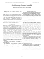
Oscilloscope Control with PC
Roland Szabó, Aurel Gontean, Ioan Lie, Mircea BăbăiŃă
II. PROBLEM FORMULATION
Abstract—In this paper two different oscilloscope control
methods are presented. The first method is the classic method to send
the SCPI commands via RS232 serial interface. The second method
is to use the LabVIEW divers. The first oscilloscope is the HAMEG
HM407, which has its control program implemented in MATLAB.
The second oscilloscope is the NI PXI-5412 with the control program
in LabVIEW. The second control program is much faster and mare
simple, but with the classic method we can configure more and have
a better control over the oscilloscope. The classic method is also
general, because it can be controlled any oscilloscopes and
equipment, even if they have no driver. In the first method the driver
is made, in the second method a driver is used.
The most often used functions needed to be implemented in
the computer interface of this HAMEG HM 407 oscilloscope.
Some functions that are not possible without a computer,
like saving a graph from the oscilloscope, or sending a graph
to the oscilloscope, were the main target.
On the computer interface the buttons needed to have
similar name as those present on the oscilloscope.
III. PROBLEM SOLUTION
A. Programming Language Presentation
The goal was clear, to make a simple, but efficient
computer interface for the oscilloscope via RS232 interface.
The software used for programming was MATLAB. This
software is simple and powerful. MATLAB has also a
graphical interface, which was very useful for our
oscilloscope’s user interface creation. The only inconvenience
is that MATLAB has only Windows style controls, like
sliders, buttons, check boxes and radio buttons. When, for
example, a TIME/DIV. dial is needed, we had to use slider,
not so suggestive, but functional.
Maybe for a better user interface some National
Instrument’s software can be more convenient, like LabVIEW,
LabWindows/CVI or Measurement Studio for Visual Studio,
because these software packages have dials, LEDs, graphs and
other controls and indicators which look like the ones on
electronic equipments.
MATLAB has its own advantages too. The thing that is
very useful in MATLAB graphical interface is that any change
on button makes change immediately a change in the
MATLAB *.m code file. No need for generate callbacks like
in other programming languages like Visual Studio or
LabWindows/CVI. This can be very useful when a
complicated code is made.
Keywords—Communication equipment, control equipment,
driver, oscilloscope, protocol, remote handling, serial port.
I. INTRODUCTION
T
HIS paper presents the creation of an oscilloscope driver.
To test the driver, the HAMEG HM 407, 40 MHz,
100MS/s cathode-ray tube oscilloscope (Fig. 1.) is connected
with the PC to be controlled via the RS232 serial port. The
oscilloscope is an analog/digital oscilloscope. It has an RS232
serial port and a microcontroller with implemented SCPI
(Standard Commands for Programmable Instruments)
commands. Its commands are presented in the product
datasheet. Some commands are quite complicated and need a
lot of binary calculation to make them work. Some of them are
not complete or not well explained and need programming
tricks to make them fully functional. Some commands are
related to other commands. These dependencies are explained
in another datasheet, so to command this equipment, a lot of
prior study is needed.
The oscilloscope has a quite old microcontroller and this
makes it a little more difficult to program, then other
equipments.
Its commands are not standardized; the commands are
closer to binary code.
This equipment was chosen, because it’s not common
equipment, like the Agilent equipments, which quite really
simple to program and most of them have drivers for all
common communication ports present on an equipment, like
GPIB, RS232, USB or Ethernet.
B. MATLAB Graphical Interface
MATLAB graphical interface can be accessed when the
“guide” command is introduced at the command prompter.
This command will open a window like the one in Fig. 2.
Here the user can drag-and-drop buttons, sliders and other
Windows style controls and indicators needed.
In the oscilloscope interface sliders, Push buttons, pop-up
menus controls and edit text, axe indicators were used.
33
INTERNATIONAL JOURNAL OF COMPUTERS AND COMMUNICATIONS
Issue 3, Volume 3, 2009
Fig. 1. HAMEG HM 407 oscilloscope’s front with display and control buttons.
Fig. 2. Front panel creation of the oscilloscope in MATLAB. This window can be accessed when the “guide” command is introduced to the command prompter.
34
INTERNATIONAL JOURNAL OF COMPUTERS AND COMMUNICATIONS
As we can see we have a Connect button for connecting the
computer to the oscilloscope. This buttons sends the
command, which puts the equipment in remote mode. During
this time, the physical buttons from the oscilloscope are not
functional, it pressed they make an error beep. An LED
indicator on the oscilloscope indicates that the equipment is in
remote mode and can be commanded just with a computer. On
the graphical interface the status of the oscilloscope is shown
with and edit text indicator, where the information ON or OFF
is shown, depending on the state of the oscilloscope (remote or
local).
To return to local mode, the Autoset button from the
oscilloscope need to be pushed for a few seconds and the
oscilloscope will return in local mode. The Autoset button’s
secondary function is returning the oscilloscope in local mode.
After this operation the oscilloscope will not be commanded
eth the PC, just with the buttons physically present on the
equipment and the remote LED will be turned off. To return
the oscilloscope in local mode, the disconnect button from the
computer interface can be used too.
The Autoset button from the user interface has the same
effect as the Autoset button physically present on the
oscilloscope; it sets the Time/DIV and Volt/DIV parameters
most optimal to the acquisitioned signal.
For setting the horizontal (X-POS.) and vertical (Y-POS. I
and Y-POS. II) positions of the signal, sliders were used. Here
a little trick need to be used, because for positive vertical
position was one command and for negative vertical position
was another command, but only one slider was used, so the
two commands needed to be merged in one.
For setting the timebase (TIME/DIV.) and the amplitude
(VOLTS/DIV. I and VOLTS/DIV.), also sliders were used.
Because sliders, were fuzzy, a more accurate solution was
needed, to set exactly the timebase and the amplitude, this way
pop-up menus were used. For timebase between 1 µs/DIV.
and 0,5 s/DIV., for amplitude between 1 mV/DIV. and 20
V/DIV. The values can be set exactly. For the timebase and
amplitude, both controls are functional, for exact and for fuzzy
setting of the signal.
For saving the signal form the oscilloscope two buttons are
used Read Wavef. I (for CH I) and Read. Wavef. II (for CH
II). The signal will be shown on the axe. The acquisitioned
signal has 256 samples (256 points), for larger signals more
samples need to be combined. The serial interface has a buffer
of 512 samples.
For writing a saved waveform from the computer to the
oscilloscope, the Write Wavef. I and Write Wavef. II buttons
were used. The oscilloscope has two memories and this way it
can memorize to signals. The signals are saved in a text file
(signal.txt) as points. This can be used for saving each signal
from each channel to the computer, make some signal
processing and after that send it back to the equipment. In the
signal.txt file also is a signal with 256 samples (256 points).
Here also a little trick is needed to make it work, the
oscilloscope need to be put in STOR. MODE, so the REF bit
has to be put on “1” logic by software, otherwise it will not
work. This is very important to be done, because otherwise if
Issue 3, Volume 3, 2009
the REF bit is not activated manually on the oscilloscope, the
saving of a signal will not work and an error beep will be
received.
C. The Code behind the buttons
In this section the code behind the buttons is explained.
Every SCPI command needs to be ended with carriage
return (CR, 0Dh or 13d). There are exceptions too, some of
them needs only CR and other CR and LF, depends on the
SCPI command.
These SCPI commands can be obtained from the
oscilloscopes user manual or from an existing program with
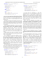
the HHD Free Serial Monitor program (Fig. 3 and Fig. 4.).
With this program we can obtain the SCPI commands that the
existing program uses.
Fig. 3. The HHD Serial Monitor program configured.
Fig. 4. The HHD Serial Monitor program obtaining SPCI commands from
and existing program.
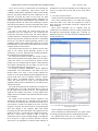
TABLE I shows the used SCPI commands.
These commands are obtained from the user guide or from
an existing program using the Free Serial Monitor program.
We obtained them from the user manual, because we
couldn't find an existing program for our oscilloscope.
35
INTERNATIONAL JOURNAL OF COMPUTERS AND COMMUNICATIONS
Command
AUTOSET
YzPOS=w
XPOS=w
CHz=b
TBA=b
STRMODE=b
RDWFMz:ww
WRREFz:ww
RM0
TABLE I
USED SCPI COMMANDS
Description
AUTO SET function will be carried out
Sets Y 1/2 POSITION settings
Sets X-POSITION settings
Sets CH1/2 settings (like amplitude)
Sets TIMEBASE A/B settings
Delivers STORE MODE
READ WAVE FORM 1/2
WRITE REFERENZ 1/2
Exit REMOTE mode
Issue 3, Volume 3, 2009
set(handles.sts, 'String', 'ON');
...
set(handles.sts, 'String', 'OFF');
Where sts is the indicator’s identifier and String is the
parameter that is changed and after that is the value: ON or
OFF. With this command almost every parameter can be
changed, like size or position.
The whole initialization program is the following:
function HM407_OpeningFcn(hObject,
eventdata, handles, varargin)
handles.obj1=serial('COM1');
handles.output = hObject;
guidata(hObject, handles);
The functions used for write and read data from the serial
port are fwrite and fread.
For example the Autoset button has the following code:
function autos_Callback(hObject,
eventdata, handles)
cmdb=double('AUTOSET');
b=[13 10];
fwrite(handles.obj1,[cmdb b]);
b1=fread(handles.obj1,3);
function varargout =
HM407_OutputFcn(hObject, eventdata,
handles)
varargout{1} = handles.output;
function axes1_CreateFcn(hObject,
eventdata, handles)
Every button has similar code to this example, obj1 is set to
COM1, the first serial port installed on the computer, but it
can be set to any COM port desired with the following
command:
function con_Callback(hObject,
eventdata, handles)
fopen(handles.obj1);
set(handles.obj1,'FlowControl','hardwa
re');
a=[32 13];
fwrite(handles.obj1,a);
a1=fread(handles.obj1,3);
set(handles.sts, 'String', 'ON');
The Disconnect button is made similar, but it uses the RM0
(remote 0) SCPI command and the serial port is closed with
the fclose function:
handles.obj1=serial('COM1');
The information is sent decimal. Comments are generated
automatically by MATLAB, which can be cleared. Here the
SCPI command is: AUTOSET. The command need to be
ended with carriage return (CR, 0Dh or 13d) and line feed (LF
0Ah or 10d) too. The AUTOSET command is concatenated
with the carriage return and line feed bits. The number 3from
the fread function is the number of bits read.
Modifying this function we can make the functions for all
buttons, just by reading the specific SCPI command from
datasheet and being attentive to some bits.
The Connect button has a similar function, but no SCPI
commands are used, only sending the 20h (32d) and the CR
termination character. The serial port is opened with the fopen
and closed with fclose functions and set to its default values:
baud rate: 9600, data bits: 8, parity: none, stop bits: 1, flow
control: none:
function discon_Callback(hObject,
eventdata, handles)
cmdz=double('RM0');
z=[13 10];
fwrite(handles.obj1,[cmdz z]);
z1=fread(handles.obj1,3);
set(handles.sts, 'String', 'OFF');
fclose(handles.obj1);
For the horizontal position setting first we read the value of
the slider with the following command:
fopen(handles.obj1);
...
fclose(handles.obj1);
yp1=get(hObject,'Value');
Then we use the YzPOS=w SCPI command, where z is the
number of channel, 1or 2 and w is the distance in word. The
only problem is that the oscilloscope is like a coordinate
system and it has positive and negative position. The goal was
to change the position with only one button, so a little trick
was needed.
The program that does the trick is the following:
The serial port is activated with the following command:
set(handles.obj1,'FlowControl','hardware
');
The ON/OFF indicator is commanded, where needed, with
the following commands:
36
INTERNATIONAL JOURNAL OF COMPUTERS AND COMMUNICATIONS
function ypos1_Callback(hObject,
eventdata, handles)
yp1=get(hObject,'Value');
cmdc=double('Y1POS=');
if (yp1>15)
cyp1=yp1-15;
end
if (yp1<=15)
cyp1=yp1+240;
end
c=[160 cyp1 13];
fwrite(handles.obj1,[cmdc c]);
c1=fread(handles.obj1,3);
Issue 3, Volume 3, 2009
The program for the timebase is the following:
function tdiv_Callback(hObject,
eventdata, handles)
timed=get(hObject,'Value');
cmdh=double('TBA=');
h=[round(timed) 13];
fwrite(handles.obj1,[cmdh h]);
h1=fread(handles.obj1,3);
For pop-up menu the programming is a little more
complicated, because we ne exact amplitude and timebase. For
amplitude, we have 14 values between 1 mV/DIV. and 20
V/DIV, this way 1 mV/DIV. means 1, but we need to send 16,
and 20 V/DIV. means 14, but we need to send 29, so we have
to add 15 to every value. Same thing for TIME/DIV. but we
have 26, values between 1 µs/DIV. and 0,5 s/DIV., so we need
to add 3 to every value.
Maybe a little more complicated is the reading of the
waveforms, the used SCPI command is RDWFMz:ww, where
z is the number of channels, 1 or 2 and the first w word is the
offset and the second is the length. The offset we will set to 0,
so the first two bytes are 00h and 00h. The length we will set
to 256 samples (256 points), the serial has a 512 sample
buffer. 256 = 0100h, we split the word in two bytes and we get
01h and 00h, after all we need to send it in reversed order, so
00h and 01h. All the numbers from the offset and length in
reversed order, in decimal and with CR termination character
is: 0 0 0 1 13.
Where we plot the information from the 12th sample,
because these samples in the start are information about the
waveform, but the waveform data starts from 12 and ends at
267.
For this signal acquisition to work we have to be careful
with the STOR. MODE bits using the STRMODE=b SCPI
command. D7 = REF2, D6 = REF1, D5 ÷ D3 = PRE
TRIGGER (011 = 0%) and D2÷D1 STOR MODE (000 =
REF). This way for signal acquisition we need no reference
memory, so we have 11000b (24d), for sending signals to
reference memory 1 we will have 1011000b (88d) and for
reference memory 2 we will have 10011000b (152d). This
way we don’t need to push the reference button manually all
the time and stop the program.
After it we need to lot de received data to the axe, so the
program section will be:
As we can see the program is similar, but with if statement
insertion. The whole idea is that the information that we have
to send is 16 bits long, so we need two decimal numbers. The
slider is set to the value of 15 and the minimum value to 0 and
maximum to 30.
The whole screen height is FF0h (4080d), the inserted string
is the LF (0Ah), so this way we have FF0Ah. We split the
word in two bytes and get FFh and 0Ah, we reverse them and
get FFh (255d) and A0h (160d), and these need to be sent in
reversed orders.
With the implemented algorithm we will be able to change
the vertical position in brute values (changing the MSB). In
binary the positive values for the second byte are between
00000000b – 00001111b (00h – 0Fh, 0d – 15d) and the
negative values between 11110000 – 11111111 (F0h – FFh,
240d – 255d), the negative values are in the complement of 2,
so the lowest value is FFh (255d) and the highest is F0h
(240d).
A same program can be made to the channel 2, but using
Y2POS=w SCPI command and for horizontal position with the
XPOS=w SCPI command.
For the amplitude the used SCPI command is CHz=b,
where z in the number of channel, 1 or 2 and b is the value in
byte. There are 4 bytes for other settings to the channel and 4
bytes for setting the amplitude. D7 = GND, D6 = AC, D5 =
INV, D4 = ON, D4 ÷ D0 are the setting for amplitude between
0000b – 1101b (0d – 13d). All bits can be “0” logic, but the
ON bit must be at “1” logic, so the number we need to send
are between 10000b – 11101b (16d – 29d). This way the
slider’s value is set to 22 and the minimum value to 16 and the
maximum value to 28.
The same thing can be made for the channel 2, but with the
CH2=b SCPI command and a similar function will work for
the timebase, but with the TBA=b SCPI command, where A is
the A timebase, because this model has no B timebase.
The program for the amplitude is the following:
function rdwf1_Callback(hObject,
eventdata, handles)
cmdi=double('STRMODE=');
i=[16 13];
fwrite(handles.obj1,[cmdi i]);
i1=fread(handles.obj1,3);
cmdj=double('RDWFM1:');
j=[0 0 0 1 13];
fwrite(handles.obj1,[cmdj j]);
j1=fread(handles.obj1,267);
l=1;
for k=12:267
function vdiv1_Callback(hObject,
eventdata, handles)
vold1=get(hObject,'Value');
cmdf=double('CH1=');
f=[round(vold1) 13];
fwrite(handles.obj1,[cmdf f]);
f1=fread(handles.obj1,3);
37
INTERNATIONAL JOURNAL OF COMPUTERS AND COMMUNICATIONS
Issue 3, Volume 3, 2009
V(l)=j1(k);
l=l+1;
end
plot(V)
For writing a signal to the memory is quite similar to
reading it. The used SCPI command is WRREFz:ww, where z
is the number of channels, 1 or 2 and the first w word is the
offset and the second is the length. The signal is written by
some numbers in one colon in the signal.txt file.
The function should be the following:
function wtwf1_Callback(hObject,
eventdata, handles)
cmdm=double('STRMODE=');
m=[88 13];
fwrite(handles.obj1,[cmdm m]);
m1=fread(handles.obj1,3);
load signal.txt -ascii;
cmdn=double('WRREF1:');
n=[0 4 0 1 signal' 13];
fwrite(handles.obj1,[cmdn n]);
n1=fread(handles.obj1,3);
The signal it’s transposed with signal’, it is more simple to
write values in a colon in a *.txt file than in a row. The file
must contain exactly 256 values (Fig. 5.).
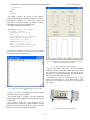
Fig. 6. The graphical user interface for the HAMEG HM 407oscilloscope
running when acquisitioning a square signal.
IV. THE NI OSCILLOSCOPE COMMAND
The NI oscilloscope differs more from the HAMEG
oscilloscope. It's not a stand-alone oscilloscope, it only a card
that can be used just connected to a PC, this way the drivers
are compulsory, so National Instruments provided them. The
drivers were used and worked very well.
The oscilloscope card is in a PXI chassis (Fig. 7.). This
chassis is connected to the PC via the MXI interface, which
has speed up to 132 MB/s. Our chassis is the NI PXI-1044
with 14 slots.
Fig. 5. The signal.txt file with some random numbers forming a random
signal.
In Fig. 6. we can see the graphical user interface running
and acquisitioning a square waveform.
The plotted signal is generated with the oscilloscope
internal generator with plugging the oscilloscope probe in the
calibrate input.
The measured signal has more samples, but we
acquisitioned only 256 samples + signal information, because
the RS-232 interface has a buffer of 512 samples. For more
samples we have to make multiple acquisitioning.
Fig. 7. NI PXI-1044 chassis for acquisition cards.
38
INTERNATIONAL JOURNAL OF COMPUTERS AND COMMUNICATIONS
Issue 3, Volume 3, 2009
Registers to make the static Waveform Graph dynamic;
otherwise we would see a graph just after the While loop ends.
The chosen oscilloscope is the NI PXI-5412 (Fig. 8.). This
oscilloscope is traditional National Instruments equipment. It
uses the NI-SCOPE driver.
Fig. 8. NI PXI-5412 oscilloscope from National Instruments.
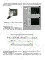
The Front Panel of the NI PXI-5412 oscilloscope command
made in LabVIEW is shown in Fig. 9. As we can see we have
the resource name, which shows the card number in the PXI
chassis. Two vertical adjust dials for each channel and a
horizontal adjust dial. We have two Waveform Graphs which
shows the signals at each channel.
The Block Diagram is shown in Fig. 10. As we can see we
have a While loop. Its timing is set to 100 ms. Outside of the
loop is the initialize and close VIs, ending everything with
simple error handler. We have one horizontal adjust VI and to
vertical adjust VIs with two read VIs for the two channels
from the oscilloscope (channel 0 and 1). At the second channel
we have a Bessel filter. We used a Build Array VI and Shift
Fig. 9. The Front Panel of the NI PXI-5412 oscilloscope program made in
LabVIEW.
Fig. 10. The Block Diagram of the NI PXI-5412 oscilloscope program made in LabVIEW.
datasheet needs to be analyzed well and with a little binary
calculation and some programming trick almost everything
can be done.
The goal was achieved. We wanted to program an
instrument and we needed some functions that are not possible
without a computer, like signal sending to the oscilloscope or
saving from it.
Further enhancements would be to make a button for every
setting on the oscilloscope, maybe try program it in other
V. CONCLUSION
These days the instruments have simple SCPI commands,
where no need for binary calculation is. Some instrument’s
vendors provide even drivers, where some functions gather the
SCPI commands with the binary values and the user just calls
the functions and enter decimal values.
As we saw almost any instrument can be programmed as
the user wants and in any programming language. The
39
INTERNATIONAL JOURNAL OF COMPUTERS AND COMMUNICATIONS
Roland Szabó is a Master student in the Faculty of Electronics and
Telecommunications, “Politehnica” University of Timişoara, România. He
was born in Timişoara, România, in April 14, 1986. He is an electrical
engineer since 2009, with LabVIEW Basics I & II Certificate from National
Instruments Hungary – 2009, with Software Quality Engineer certificate from
Continental Automotive România – 2009.
He is a Hardware Engineer at Continental Automotive România located in
Timişoara. He is research laboratory responsible in the Faculty of Electronics
and Telecommunications, “Politehnica” University of Timişoara, România.
He had summer job also in Alcatel-Lucent located in Timişoara, Romania. He
has 5 papers. Areas of interest: robots, creating computer interfaces for
electronic equipments, servers, web programming.
Eng. Roland Szabó is a Hardware Engineer at Continental Automotive
România.
programming language, like C, and make an official driver
with all function of the oscilloscope, so this way programmers
will not have to do so many binary calculations and read all
the datasheets.
The whole idea of this oscilloscope programming is that we
wanted to see if we are capable of programming an
oscilloscope with complicated SCPI commands with binary
calculations.
With this knowledge now we are capable communicating
with almost any equipment. It’s an old equipment, but it still
needs to be connected to the computer and it still needed to be
programmed. As mentioned in the introduction these older
equipments are still needed. On the other hand, somebody
needs to make drivers for the instruments for simpler
programming. This paper’s goal is to show how to interpret
the SCPI commands and this way to make an instrument
driver. This paper is just an example how to program more
complicated instruments. With this knowledge we hope that
the communication with instruments will not be a problem.
Aurel Gontean is professor and vicedean in the Faculty of Electronics and
Telecommunications, “Politehnica” University of Timişoara, România. He
was born in June 26, 1961. He had 3 months scholarship at Central Lancashire
University, Preston, England, VLSI Design oriented – 1996, a 3 months
scholarship at Fachhochschule Wiesbaden, Germany, Programmable Logic
Design oriented – 1995, a 3 days FPGA Workshop, Texas Instruments,
Germany – 1993. He is an IEEE member since 1999.
Activities: Invited Professor, DH Loerrach, Germany, EU Expert –
appointed grant reviewer in Bulgaria, Initiates the Remote Access Electronic
Lab in Electronics Faculty Timişoara, România, International Program
Committee member, Programmable Devices and Systems conferences, IFAC,
National reviewer for Romanian grants, Workshops and trainings dedicated to
Digital Electronics Fundamentals and Microcontrollers at Solectron,
Timişoara, Workshops and trainings dedicated to Digital Electronics
Fundamentals and Microcontrollers at Siemens VDO, Timişoara, IEEE
Member, 1994 - Member in the π - TEAM (research team), Texas
Instruments, Europe, 1993 Appointed lecturer for Texas Instruments FPGA
Workshops and Seminars in Romania. He has over 70 papers, 5 books and
over 20 grants. Interests: VHDL, FPGA, C.NET programming.
Prof. Aurel Gontean, PhD is a PhD advisor in the Faculty of Electronics
and Telecommunications, “Politehnica” University of Timişoara, România.
REFERENCES
[1]
[2]
[3]
[4]
[5]
[6]
[7]
[8]
[9]
[10]
[11]
[12]
[13]
[14]
Issue 3, Volume 3, 2009
N. Sulaiman, N. A. Mahmud, “Designing the PC-Based 4-Channel
Digital Storage Oscilloscope by using DSP Techniques,” Research and
Development, 2007. SCOReD 2007. 5th Student Conference, 2007, pp.
1–7.
Tew Yiqi, Goi Bok-Min, “Oscilloscope: A PC-based Real Time
Oscilloscope,” Innovative Technologies in Intelligent Systems and
Industrial Applications, 2008. CITISIA 2008. IEEE Conference, 2008,
pp. 92–97.
R. Lincke, I. Bull, A. Trutia, B. Logofatu, “PC-based oscilloscope,”
Semiconductor Conference, 1995. CAS'95 Proceedings, 1995
International, 1995, pp. 229–232.
M. O. Hagler, D. Mehrl, “A PC with sound card as an audio waveform
generator, a two-channel digital oscilloscope and a spectrum analyzer,”
Education, IEEE Transactions, vol. 44. 2001.
C. Bhunia, S. Giri, S. Kar, S. Haldar, P. Purkait, “A low-cost PC-based
virtual oscilloscope,” Education, IEEE Transactions, vol. 47, 2004, pp.
295–299.
S. A. Chickamenahalli, A. Hall, “Interfacing a digital oscilloscope to a
personal computer using GPIB,” Frontiers in Education Conference,
1997. 27th Annual Conference. 'Teaching and Learning in an Era of
Change'. Proceedings, vol. 2, 1997.
MATLAB – Creating Graphical User Interfaces
MATLAB – Instrument Control Toolbox 2 User’s Guide
HAMEG Instruments – Description of Interface Commands
Muhammad Sharfi Najib, Mohd Shawal Jadin, Mohd Razali Dau,
“Development of Real-Time Signal Generator Graphical User Interface
Using Matlab 6.5,” Software Engineering, Parallel and Distributed
Systems. SEPADS '08. 7th WSEAS International Conference, 2008, pp.
103–106.
Vladislav Slavov, Tasho Tashev, “Data Acquisition Units Using For
Student Labs,” System Science and Simulation in Engineering, 5th
WSEAS International Conference, 2006, pp. 228–231.
S.M. Potirakis, M. Rangoussi, G.E. Alexakis, “Exploiting Multimedia
for the instruction of Analog Electronics, Applied Acoustics and
Electro-Acoustics undergraduate courses,” WSEAS International
Conference.
A. Etxebarria, R. Bárcena, “Real Experiments Remotely Controlled
Through The World Wide Web,” Engineering Education. EE'08. 5th
WSEAS / IASME International Conference, 2008, pp. 259–264.
A. Ascia, B. Ando’, S. Baglio, N. Pitrone, “Teaching Advanced
Technologies to Undergraduates,” Engineering Education. EE'08. 5th
WSEAS / IASME International Conference, 2008, pp. 360–365.
Ioan Lie is associate professor in the Faculty of Electronics and
Telecommunications, “Politehnica” University of Timişoara, România. He
was born in Recea, Braşov, România in October 28, 1961. Other jobs:
Engineer at “Electrotimis” Ltd. Timişoara, Timteh Electronics Ltd. Company
(Timişoara, România), The direct customers of Timteh Ltd. was Rada
Electronic Industries, Tel Aviv, Israel and Elbit Systems Ltd. Haifa, Israel.
Activities: development and implementation of software for testing Boeing
737, Boeing 777, DC-10 and Concorde airplane electronics units on the
specific Automatic Test Equipment (ATE), development and implementation
of hardware for digital video recorder, collaboration with Metrys Gmbh,
Germany, regarding Hardware and Software solutions for: Water Meters, Heat
Costs Allocators, Transit-Time Ultrasonic Liquid Flow Meters, AMR
(Automatic Meter Reading) and RFID. He has over 30 papers, 2 books and 8
grants. Interests: Electronic Design Automation, Methods and
Implementations for Ultrasonic Measurement and Testing, Programmable
Logic, Microcontrollers and Microprocessors, Automatic Test Equipments,
Software for applications
Assoc. Prof. Ioan Lie, PhD is at Applied Electronics Department, Faculty
of Electronics and Telecommunications, “Politehnica” University of
Timişoara, România.
Mircea BăbăiŃă is lecturer in the Faculty of Electronics and
Telecommunications, “Politehnica” University of Timişoara, România. He
was born in Orăştie, Hunedoara, România in July 18, 1964. He had 6 weeks
scholarship at University of Strathclyde, Glasgow, Scotland – 2000, 2 weeks
scholarship at University of Mannheim, Germany – 2002.
Activities: development and implementation of hardware and software for
regarding DSP Utilization for MCC Motor Drives, development and
implementation of hardware and software for E-learning Distance Interactive
Practical Education in Power Electronics. He has over 50, 6 books and over
20 grants. Interests: Digital Logic, Microcontrollers and Microprocessors,
Power Electronics, Motor Drives, Fuzzy Logic.
Lect. Mircea BăbăiŃă is at Applied Electronics Department, Faculty of
Electronics and Telecommunications, “Politehnica” University of Timişoara,
România.
40