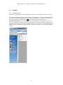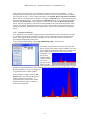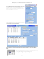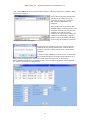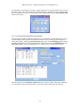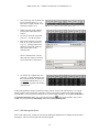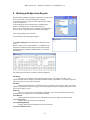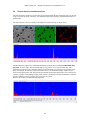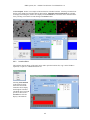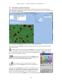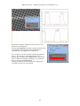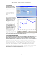
Download Iridium Ultra Version 1.4 Software User`s Guide

IXRF Systems, Inc. 3019 Alvin DeVane Blvd. Suite 130, Austin, TX 78741 • 512-386-6100 • Fax 512-386-6105
Web: www.IXRFsystems.com
E-mail: [email protected]
Iridium Ultra Version 1.4
Software User's Guide
7 February 2012
Japan only:
The power cable packed in the carton is used exclusively for the
included EDS system.
IXRF Systems, Inc. – Iridium Ultra Software User's Manual Rev 1.4
This page intentionally blank
2
IXRF Systems, Inc. – Iridium Ultra Software User's Manual Rev 1.4
Table of Contents
1. Introduction .......................................................................................................................................... 7 2. Customer Support ................................................................................................................................ 8 2.1 Contacting Us................................................................................................................................ 8 2.2 Software Updates .......................................................................................................................... 8 3. Application Overview ........................................................................................................................... 9 3.1 TitleBar ....................................................................................................................................... 10 3.2 ToolBar ....................................................................................................................................... 11 3.3 Menus.......................................................................................................................................... 13 3.4 File Menu .................................................................................................................................... 13 3.4.1 New ........................................................................................................................................ 13 3.4.2 Open. ...................................................................................................................................... 13 3.4.3 Save EDS Data Set ................................................................................................................. 14 3.4.4 Set Sample Name.................................................................................................................... 14 3.4.5 Image Browse ......................................................................................................................... 15 3.4.6 Image Batch Export ................................................................................................................ 15 3.4.7 Setup Export Formats ............................................................................................................. 16 3.4.8 Close ....................................................................................................................................... 16 3.4.9 Close All ................................................................................................................................. 16 3.4.10 Save .................................................................................................................................... 17 3.4.11 Save As .............................................................................................................................. 17 3.4.12 Export ................................................................................................................................. 17 3.4.13 Print .................................................................................................................................... 17 3.4.14 Print Preview ...................................................................................................................... 17 3.4.15 Print Setup .......................................................................................................................... 17 3.4.16 Exit ..................................................................................................................................... 17 3.4.17 Create Word Report ........................................................................................................... 18 3.5 View Menu.................................................................................................................................. 19 3.5.1 Interactive Help ...................................................................................................................... 19 3.5.2 Folders Panel .......................................................................................................................... 20 3.5.3 Application Look .................................................................................................................... 21 3.6 Tools Menu ................................................................................................................................. 21 3.6.1 System Setup User Interface ................................................................................................... 21 3.6.2 System Setup Security ............................................................................................................ 22 3.6.3 System Setup Options ............................................................................................................. 22 3.7 Window Menu ............................................................................................................................ 23 3.7.1 Cascade ................................................................................................................................... 23 3.7.2 Tile.......................................................................................................................................... 23 3.7.3 Arrange Icons ......................................................................................................................... 23 3.8 Help Menu .................................................................................................................................. 23 3.8.1 Help Topics ............................................................................................................................ 23 3.8.2 About… .................................................................................................................................. 23 3.8.3 View Release Notes… ............................................................................................................ 23 3.9 Data Protection............................................................................................................................ 24 4. Working With Spectra ....................................................................................................................... 25 4.1 Acquiring Spectra ....................................................................................................................... 26 4.1.1 Returning to Acquisition Location ......................................................................................... 26 4.2 Viewing Tools ............................................................................................................................. 26 4.2.1 Expanding and Contracting views .......................................................................................... 26 4.2.2 Auto Vertical Scale ................................................................................................................. 27 4.2.3 Manual Setting of Displayed Energy ...................................................................................... 27 4.2.4 Bipolar Display ....................................................................................................................... 27 4.3 Overlaying Spectra...................................................................................................................... 28 4.4 Annotations and Notes ................................................................................................................ 29 4.5 Customizing Display and Printing Colors ................................................................................... 31 4.6 Painting Windows ....................................................................................................................... 32 3
IXRF Systems, Inc. – Iridium Ultra Software User's Manual Rev 1.4
4.7 Identifying Peaks ........................................................................................................................ 32 4.7.1 Element ID Buttons ................................................................................................................ 32 4.7.2 Periodic Table ......................................................................................................................... 33 4.7.3 Scrolling Peak Identifier ......................................................................................................... 33 4.7.4 Cursor Identification ............................................................................................................... 34 4.7.5 Customizing Display of MLK markers .................................................................................. 34 4.7.6 Automatic Element Identification ........................................................................................... 35 4.7.7 Configuring Automatic Identification .................................................................................... 35 4.8 Customizing Spectrum Rendering for Printing, Exporting, and Clipboard................................. 36 4.9 Exporting Files ............................................................................................................................ 37 4.9.1 File/Export/Spectrum.............................................................................................................. 38 4.9.2 File/Export/Analysis ............................................................................................................... 38 4.9.3 File/Export/Multi-Spectrum Export ........................................................................................ 38 4.9.4 File/Export/Export to Word .................................................................................................... 38 4.10 Quantitative Analysis of Spectra ................................................................................................. 39 4.10.1 Analysis Settings ................................................................................................................ 40 4.10.2 Using Stoichiometry (Oxides, etc) ..................................................................................... 42 4.10.3 Minimum Intensity Criteria ................................................................................................ 44 4.10.4 Sample Coating and Thickness. ......................................................................................... 44 4.10.5 Customizing Report Output................................................................................................ 45 4.10.6 Using the Manual Processing Tool .................................................................................... 46 4.10.7 Background Modeling ........................................................................................................ 47 4.10.8 Background File ................................................................................................................. 49 4.10.9 Selection of Element Analysis Lines .................................................................................. 49 4.10.10 Gaussian Deconvolution .................................................................................................... 52 4.11 Detector Geometry ...................................................................................................................... 54 4.11.1 On-Axis Detector Setup ..................................................................................................... 55 4.11.2 Off-Axis Detector Geometry .............................................................................................. 56 4.12 Detector Setup ............................................................................................................................. 57 4.12.1 Window Parameters ........................................................................................................... 57 4.12.2 Detector Parameters ........................................................................................................... 58 4.13 ZAF Quantitative Analysis using Standards ............................................................................... 59 4.13.1 Standardless vs. Standards ................................................................................................. 59 4.13.2 Calibrations ........................................................................................................................ 60 4.13.3 Creating a ZAF Calibration File ......................................................................................... 60 4.13.4 Performing ZAF Quantitation with Standards.................................................................... 64 4.13.5 ZAF Warnings and Errors .................................................................................................. 65 4.14 Match Analysis ........................................................................................................................... 66 4.14.1 Qualitative Match Analysis ................................................................................................ 67 4.14.2 Quantitative Match Analysis .............................................................................................. 69 4.14.3 Viewing Match Results ...................................................................................................... 70 4.15 Least-Squares quantitation method ............................................................................................. 71 4.15.1 Creating the calibration file ................................................................................................ 71 4.15.2 Quantifying with Least Squares ......................................................................................... 77 4.16 Material Classification ................................................................................................................ 80 4.16.1 Enable Materials Classification .......................................................................................... 81 4.16.2 Select or Create a Database ................................................................................................ 82 4.16.3 Select or Create a Materials Class ...................................................................................... 82 4.16.4 Edit Materials in Materials Class ....................................................................................... 82 4.16.5 Test the Materials Class with Samples ............................................................................... 83 4.16.6 Setting Minimum Counts in Spectrum ............................................................................... 84 4.17 Spectrum Simulation ................................................................................................................... 84 5. Working with Automatic Multiple Spectrum Acquisition .............................................................. 85 5.1 Selecting Locations ..................................................................................................................... 85 5.2 Adding Labeled Locations .......................................................................................................... 85 5.3 Selecting Analysis Settings ......................................................................................................... 86 4
IXRF Systems, Inc. – Iridium Ultra Software User's Manual Rev 1.4
5.4 Selecting Location for File Storage............................................................................................. 86 5.5 Selecting Report Output Options ................................................................................................ 86 5.6 Starting the Analysis ................................................................................................................... 86 5.7 Saving and Loading Location Files............................................................................................. 86 6. Working with Spectrum Reports ...................................................................................................... 87 7. Working with Combined SEM/XRF spectra ................................................................................... 89 7.1 Acquiring Spectra ....................................................................................................................... 90 7.2 Identifying Peaks ........................................................................................................................ 90 7.3 Quantifying Spectra .................................................................................................................... 90 8. Working With VP Spectra ................................................................................................................. 92 8.1 Enabling VP Quantitation ........................................................................................................... 92 8.2 Acquiring VP Spectra ................................................................................................................. 92 8.3 Quantifying VP Spectra .............................................................................................................. 93 9. Working With X-ray Maps ................................................................................................................ 94 9.1 Acquiring An X-ray Map ............................................................................................................ 94 9.1.1 Preparing the microscope and EDS system for acquisition .................................................... 94 9.1.2 Creating and Acquiring the X-ray map................................................................................... 94 9.2 Setting Acquisition Properties..................................................................................................... 95 9.2.1 Returning to Acquisition Location ......................................................................................... 96 9.3 Setting Element Properties .......................................................................................................... 96 Adjusting Color Palettes for X-ray Maps ................................................................................................. 98 9.3.2 Setup Palette Files .................................................................................................................100 9.4 Spectral Imaging ........................................................................................................................101 9.5 View Histogram .........................................................................................................................102 9.6 The Sum Spectrum and Maximum Pixel ...................................................................................103 9.6.1 Element Selection ..................................................................................................................104 9.7 Exporting X-ray Maps ...............................................................................................................104 9.8 Viewing Intensity/Composition of Points on X-ray Maps .........................................................105 9.8.1 Modes ....................................................................................................................................106 9.8.2 Locations Menu .....................................................................................................................107 9.9 Overlaying X-ray Maps (Composites) .......................................................................................108 9.10 Element Quantitative X-ray Maps .............................................................................................109 9.11 Component Quantitative X-ray Maps ........................................................................................110 9.12 Viewing Quantitative Maps .......................................................................................................110 9.13 Quantifying X-ray Maps (Composition) ....................................................................................111 9.14 Scatter Plot Analysis ..................................................................................................................113 9.15 Extracting Linescans from Maps ...............................................................................................114 9.16 Annotating Maps ........................................................................................................................114 9.17 3D Viewer ..................................................................................................................................115 9.17.1 3D Control Panel ...............................................................................................................117 9.17.2 Color Control Panel...........................................................................................................118 9.17.3 Zoom Control Panel ..........................................................................................................119 9.17.4 3D Menu............................................................................................................................119 9.18 X-ray Map Drift Correction .......................................................................................................119 9.18.1 Enabling Drift Correction..................................................................................................121 9.18.2 Acquiring Maps with Drift Correction ..............................................................................121 10. Working with X-ray Linescans ...................................................................................................123 10.1 Acquiring X-ray Linescan ..........................................................................................................123 10.1.1 Preparing the microscope and EDS system for acquisition ...............................................123 10.1.2 Creating and Acquiring the X-ray linescan .......................................................................124 10.2 Setting Acquisition Properties....................................................................................................124 10.2.1 Returning to Acquisition Location ....................................................................................125 10.3 Setting Element Properties .........................................................................................................125 10.4 Viewing Intensities and Concentrations.....................................................................................126 10.5 Overlay Linescans ......................................................................................................................128 10.5.1 Intensities or Concentrations .............................................................................................129 5
IXRF Systems, Inc. – Iridium Ultra Software User's Manual Rev 1.4
10.5.2 Overlay On Image .............................................................................................................129 10.5.3 Export, Print, and Clipboard..............................................................................................129 10.6 Printing Linescans ......................................................................................................................129 10.6.1 Single Page Output Style...................................................................................................129 10.6.2 Multi-Page Output .............................................................................................................129 11. RoboStage .....................................................................................................................................130 12. Stitched Images and Stitched Maps ............................................................................................132 12.1 Acquisition .................................................................................................................................132 12.2 Editing ........................................................................................................................................134 12.3 Saving and Exporting .................................................................................................................135 13. WDX Support ...............................................................................................................................136 14. Energy Calibration .......................................................................................................................137 14.1 Offset DAC Calibration (Model 500 only) ................................................................................137 14.2 Manual Energy Calibration and Threshold Adjustments ...........................................................138 14.3 Automatic Energy Calibration ...................................................................................................140 14.4 Low Energy Calibration .............................................................................................................141 14.5 View Input .................................................................................................................................143 14.6 Calculating Detector FWHM .....................................................................................................143 6
IXRF Systems, Inc. – Iridium Ultra Software User's Manual Rev 1.4
1. Introduction
Welcome to the EDS system from IXRF Systems, Inc. This combination of hardware and
software is a powerful, yet easy-to-use system encompassing all aspects of x-ray microanalysis and
optionally, XRF (X-Ray Fluorescence). Because of the technology used, Energy-Dispersive Spectrometry,
this technique is often referred to as EDS analysis. The purpose of this software is to acquire and analyze
x-ray spectra, x-ray maps and linescans, and electron images, to perform a complete analytical analysis of a
sample located in a Scanning Electron Microscope (SEM) or Transmission Electron Microscope (TEM).
Operating on all of the current Microsoft operating systems (Windows 2000, Windows XP, Vista, and
Windows 7), the EDS software seamlessly integrates with many other powerful applications to provide
custom report generation and connectivity with other networked systems.
The purpose of this manual is to describe the common activities that the EDS software is designed
to perform. As such, the primary chapters are titled “Working with …”. It is assumed that you are familiar
with the basics of operating a Windows application and that you are familiar with the common terms and
techniques of EDS analysis. If you are not familiar with Windows applications it is recommended that you
review the “Getting Started” book which is provided with your computer system, and is also available from
the Help menu item on your computer desktop. To gain familiarity with EDS analysis, the following books
are recommended:
• “Scanning Electron Microscopy and X-Ray Microanalysis,” 2nd Edition, by J. I. Goldstein,
D. E. Newbury, P. Echlin, D. C. Joy, A. D. Romig, Jr., C. E. Lyman, C. Fiori and E. Lifshin,
Plenum Press, New York (1992).
• “Quantitative Electron-Probe Microanalysis,” 2nd Edition, by V. D. Scott, G. Love and
S. J. B. Reed, Ellis Horwood Ltd., Hemel Hempstead, UK (1995).
• “Quantitative X-Ray Spectrometry,” 2nd Edition, by R. Jenkins, R. W. Gould and D. Gedcke,
Marcel Dekker, Inc., New York (1995).
7
IXRF Systems, Inc. – Iridium Ultra Software User's Manual Rev 1.4
2. Customer Support
We are committed to supporting our customers. Support can be accessed via telephone, fax, or 24-hours a
day via the internet.
2.1 Contacting Us
We can be contacted by:
Telephone: +1- 512-386-6100 from 9:00AM to 5:00PM Central Standard (or Daylight) Time.
FAX: +1-512-386-6105
Email: [email protected]
Internet: www.IXRFsystems.com
2.2 Software Updates
We provide free, lifetime updates to the original purchaser of the EDS application software via our web
site. This is a complete installation package for the software. To access the latest release of the software,
do the following:
• With your internet browser, go to the web site, http://www.IXRFsystems.com.
• Click on the Support button at the top of the home page.
• Click on the Downloads button on the left side of the Support .
• Please read carefully the instructions or Release Notes on the Software Downloads page. The
instructions on this page may change as new releases are provided. For example, a new driver for
the MCA card may be required, and this may require additional steps to be taken to complete the
installation of the latest software.
• A password is required for most of our software and user manuals installations. To obtain the
password, contact us by telephone as described in Contacting Us.
The software update installation is typically a two-step procedure:
1. Download the software. If you have replaced your computer, you will need to download
and install the Support Files.EXE. These files MUST be installed prior to the EDS
application.
2. Run the installation software. Typically, this installs the software automatically,
overwriting the previous version.
Some Internet connections have firewall protection, which may prevent downloading of software from the
Internet. If you have difficulty downloading the software from our web site, please contact your network
manager to acquire the access rights necessary to download. Administrator rights may also be required on
the computer.
8
IXRF Systems, Inc. – Iridium Ultra Software User's Manual Rev 1.4
3. Application Overview
All acquisition and analysis tools provided by the EDS software are contained in a single application.
Shown above is an example of the four major tools provided by the software:
• Digital Images
• EDS or XRF spectra
• X-Ray linescans
• X-Ray maps
Each one of these tools is loaded as necessary.
9
IXRF Systems, Inc. – Iridium Ultra Software User's Manual Rev 1.4
3.1
TitleBar
TitleBar
Menu Bar
ToolBar
At the top of the application is a TitleBar. Displayed in the TitleBar are the name of the application and the
name of the active window (Spectrum1, in this case). As you work with the software, you activate a
window by clicking on it with the left mouse button. Activating a window will do the following:
• Place the name of the active window in the TitleBar
• Update the menu. Each type of window (spectrum, image, etc) has its own unique menu designed
specifically for the kind of window.
• Update the status of the ToolBar buttons. Only the buttons that apply to the active window will be
enabled, all other buttons will be deactivated, and will be displayed “grayed out”. An example of
a disabled button is seen on the far right side of the ToolBar. The button is not active for the
spectrum window.
10
IXRF Systems, Inc. – Iridium Ultra Software User's Manual Rev 1.4
3.2 ToolBar
The ToolBar contains buttons to perform common tasks, and displays status information during spectrum
acquisition. Below is a brief description of each item on the ToolBar.
Creates a new active window (e.g.
Spectrum, Image)
Prints the active window
Opens a previously stored Spectrum,
Image, etc from disk
Displays information about the software
Stores the active window (Spectrum,
X-ray Map, etc) on one of the system's
disks
Creates a new combined SEM/XRF
spectrum.
Creates a new spectrum and start
acquisition of the spectrum
Copies the active window (e.g.,
Spectrum, Image) to the Windows
Clipboard
Creates a Fast Map using the element
list of the spectrum and start acquiring
the Fast Map
Creates a new Image and start acquisition
of the image
Toggles Spectrum Auto Vertical
Scaling
Expands the spectrum Vertical Scale
Contracts the spectrum Vertical Scale
Compresses the spectrum horizontally
Expands the spectrum horizontally
Enables display of the energy cursor on
the spectrum
Enables the painting of an ROI on the
spectrum
Performs Automatic Element
Identification
Erases Automatic Element
Identification
Displays the Periodic Chart for manual
element identification
Closes all opened windows.
Creates a Fast Linescan using the element
list of the spectrum and start acquiring the
Fast Linescan.
Toggles display of Spectrum Analysis
Report.
Enables annotation on the spectrum or
image
Performs Quantitative analysis of the
spectrum
Selects a new set of default analysis
settings
Image: selects spot location.
Linescan: selects horizontal line
Displays or Hides Interactive Help
panel.
For images, selects a freehand area for
acquisition of a spectrum.
For linescans, selects an arbitrary line
on the image for acquisition.
For images, selects a reduced raster area
for acquisition of a spectrum.
For images, selects an area for
acquisition of an x-ray map.
For images, selects a line for acquisition
of an x-ray linescan.
11
IXRF Systems, Inc. – Iridium Ultra Software User's Manual Rev 1.4
The bottom half of the ToolBar contains controls and status readouts used for acquiring data. These
controls are described below.
Acquire Start/Stop. This button starts and stops acquisition on the active window (e.g.,
Spectrum, Image, X-ray Map). During acquisition, the button text is changed to Stop to indicate that the
action taken when the button is pressed is to stop acquisition.
Spectrum Preset Value. This is the preset value in livetime seconds or total
counts in the spectrum. Acquisition will automatically stop when the preset condition occurs. The
Spectrum Preset Mode determines whether the value is livetime seconds or counts.
Spectrum Preset Mode. This selects the kind of Preset to use. For Livetime, the
spectrum is acquired for the given number of seconds of livetime. For Counts, the spectrum is acquired
until the specified number of x rays has been acquired (total counts in the spectrum).
Spectrum Acquire Livetime. During acquisition of the spectrum this control displays
the livetime seconds. This is the clock time that is corrected for deadtime.
Spectrum Deadtime Meter. This continuously displays the deadtime percentage. A
bar graph and a numeric readout are displayed. Deadtime is the time that the pulse processor is unable to
process incoming x-ray events, as it is already processing a prior event.
Spectrum CountRate. This continuously displays the input countrate.
Time Constant. The time constant can be set directly from here. This is the time
constant that will be used for all subsequent data acquisition (spectra, x-ray maps, x-ray linescans).
Microscope kV. Enter the accelerating voltage (kV) of the microscope in this box prior to
acquiring a spectrum, X-ray Map, or X-ray Linescan. This value is used by the software to control the
analysis of the acquired data. It is very important that this value be entered prior to acquiring the data. On
systems with microscope control, the kV is automatically read from the microscope.
Microscope Magnification. Enter the magnification of the microscope in this control
prior to acquiring an Image. The value in this control is stored in the image at the beginning of acquisition
of the image. All image measurements are based upon this value, so it is very important that it be correct
for any measurements to be calculated correctly. On systems with microscope control, the magnification is
automatically read from the microscope.
Active Stage. For systems with an IXRF Super Stage, or other
supported secondary stage, the active stage is selected here. The active stage is used for image and map
stitching, and stage maps and stage linescans. The full stage position is saved with all data acquired with
12
IXRF Systems, Inc. – Iridium Ultra Software User's Manual Rev 1.4
the EDS software (both active stage and microscope stage). This allows for accurate repositioning of the
stage(s) to review acquired data locations.
3.3 Menus
A unique menu is displayed for each kind of window. There are, however, some common menu items that
are applicable to all windows. These are described below.
Throughout this manual, references will be made to items on the menu. The style will be:
MenuItem/SubMenuItem
MenuItem appears on the menu directly, at the top of the application and when the right mouse button is
clicked over a window (e.g., Spectrum, X-ray Map). Selecting MenuItem will display a drop-down (sub)
menu. For example, the menu shown below for the Open submenu item on the File menu would be
referenced as File/Open.
3.4 File Menu
The File menu is shown to the right. All of these menu
items are common to Spectra, Images, X-ray Maps, and
Linescans. Notice that an icon (picture) is displayed to the
left of some of the menu items. The icon is a reminder that
this menu item is also available from the ToolBar by
pressing the corresponding button.
The menu items listed below Print Setup are special.
These menu items are numbered 1, 2, 3, etc and have a file
name next to each of them. These are the most recently
opened files. Selecting one of these will automatically open
the file, as if you had selected Open from the menu.
3.4.1 New
Creates a new active window (e.g. Spectrum, Image). A panel similar to the following will appear. Select
the type of file desired.
3.4.2
Open.
Opens one or more previously stored Spectrum, Image, EMSA-format spectra files, etc from disk. To open
multiple files, use the control and shift keys, as with common windows list selections.
13
IXRF Systems, Inc. – Iridium Ultra Software User's Manual Rev 1.4
3.4.3 Save EDS Data Set
Saves all opened EDS data to an EDS data set file, so that data from an analysis may be logically grouped
together in a single file.
3.4.4
Set Sample Name
Allows for setting of a sample name.
A panel similar to the following will appear. The text
entered as Sample Name will be used to name all
subsequent data acquired in the software (e.g., spectra,
images, maps, linescans). In the above example, the data
are given names of “IXRF Calibration Std-1”, “IXRF
Calibration Std-2”, etc. The Preset Index is the current
number that is suffixed to the Sample Name. In this
example, “2” is the next number. The index can be reset to restart the suffix to “1” if desired by clicking on
the Reset Index button.
The present Sample Name is displayed on the application status bar (at the bottom of the application
window), as shown below.
Double-clicking over the Sample Name on the status bar will display the panel for editing the Sample
Name, just as the File/Set Sample Name menu item does.
14
IXRF Systems, Inc. – Iridium Ultra Software User's Manual Rev 1.4
3.4.5 Image Browse
Displays images as thumbnails.
Click on Select Folder to change
the folder from which images
are displayed. Click on an
image to select it.
3.4.6 Image Batch Export
Exports multiple Image
files automatically.
Select one or more image files (use the shift key to select multiple files).
Select With Annotations to include the annotations on the images (e.g., magnification, micron scale bar,
any annotations such as text, drawing objects, etc.).
Choose the Export Image File Format and the folder in which the exported images will be Saved In.
15
IXRF Systems, Inc. – Iridium Ultra Software User's Manual Rev 1.4
3.4.7 Setup Export Formats
Allows for selection of image file formats for the export panels. Throughout the software there are options
to save data in a graphic image file format such as TIFF or JPEG. The software supports export to over 40
file formats. This setup allows the user to select only the formats that they use, thus reducing the
complexity of selecting a file format for export.
The list below is an example from an Export panel in the software. Listed are JPEG, TIF 24, and Windows
BMP 24 formats. All of the other formats are still available, and can be added to the list with the Setup
Export File Formats menu item.
Selecting Setup Export File Formats displays a panel similar to the following:
Select the formats that you want to use from the
list on the left. Click Select All to select all of
the file formats; click Remove All to de-select all
of the file formats.
3.4.8 Close
Closes the active window.
3.4.9 Close All
Closes all windows.
This menu item has the same function as the
toolbar button
.
Select the windows that you wish to close from the
list. The Action column shows the close action
that will be done for each window. By default, any
window that has been acquired and not saved will
be saved automatically before closing. The data
will be saved in the Current Folder.
Note in the example, that Spectrum1 action is No
Action Required. This is because Spectrum1 has
already been saved, and does not require saving
before closing. The other data shown (FastMap1,
FastLinescan1, etc) have not been saved, and the
default action (Save Automatic) will be applied.
16
IXRF Systems, Inc. – Iridium Ultra Software User's Manual Rev 1.4
The actions are:
• Save Automatic. Saves the data in the Current Folder using the Name given.
•
Save As. Displays a Save dialog for the data, allowing you to select a different name and folder
for the data.
•
Don’t Save. This will close the data without saving it. The previously acquired data will be lost.
•
No Action Required. This is the default setting for data that has already been saved. It is
equivalent to Don’t Save.
3.4.10 Save
Saves the contents of the active window using the name in the application TitleBar.
3.4.11 Save As
Saves the contents of the active window, allowing you to change the name of the file.
3.4.12 Export
Saves the active window in an image format. Many graphic image file formats are available including
TIFF, JPEG, and Windows Bitmap.
3.4.13 Print
Prints the active window.
3.4.14 Print Preview
Displays the active window as it will be printed. This can be used to preview the printed data prior to
actually printing it.
3.4.15 Print Setup
Provides Windows standard printer setup. A selection of printer and printer options is provided.
3.4.16 Exit
Closes all active windows and exits the EDS application.
17
IXRF Systems, Inc. – Iridium Ultra Software User's Manual Rev 1.4
3.4.17 Create Word Report
Displays a panel similar to the following. Word documents can be created and saved using this panel. All
presently opened images, spectra, x-ray maps, and x-ray linescans can be inserted into the document as well
as analyses generated from the data.
Note: this requires prior installation of Microsoft Word 2000 or newer software on the computer that is
running our EDS software.
The tree on the left side of the panel displays all of the opened data. The panel on the right is the Word
document. The controls on the toolbar on the right side can be used to directly edit the Word file.
Place In Report will take the selected data from the tree on the left side and insert it into the Word file.
From the File menu are the following features:
Save As. Saves the Word document
Open. Opens a Word document. This clears the present Word document and then loads the selected Word
file. See Insert below if you wish to add an existing Word document.
From the Insert menu is the following feature:
Word File. This inserts a selected Word file at the end of the Word document (right side of panel).
18
IXRF Systems, Inc. – Iridium Ultra Software User's Manual Rev 1.4
3.5
View Menu
3.5.1 Interactive Help
The Interactive Help panel is normally displayed on the left side of the application workspace, as shown.
This panel provides help for using the major functions of the application. Clicking on the highlighted text
or icon provides detailed, guided help for working with spectra, images, x-ray maps, and linescans. The
panel can be displayed or hidden with the
button on the toolbar or with the menu item
View/Interactive Help. You can switch from the Interactive Help panel to the Folders panel (see next
section) by clicking the tabs at the bottom of the panel. The panels can be auto-hidden by clicking on the
pushpin icon near the upper right corner of the panel (next to the “X” close icon). You can also change the
behavior and view of the panels by right-clicking on “Interactive Help/Folders” the title bar and using the
submenu.
19
IXRF Systems, Inc. – Iridium Ultra Software User's Manual Rev 1.4
3.5.2 Folders Panel
The Folders panel is also displayed on the left side of the EDS application
workspace, as shown.
This panel is used to navigate the file system and to open spectra, image,
x-ray map, and linescan files. The panel can be displayed or hidden from
the menu item View/Folders.
Operation of this panel is identical to that of the Windows Explorer.
Clicking on the + next to a drive or folder will expand the display,
showing the files and folders within; clicking on the – will collapse the
display.
Only EDS data files (spectra, images, x-ray maps, and linescans) are
displayed in this panel. To open any of these files, double-click on the
file.
20
IXRF Systems, Inc. – Iridium Ultra Software User's Manual Rev 1.4
3.5.3
Application Look
The Application Look menu item is only
shown when the EDS application is initially
opened and there are no data displayed;
where only a blank workspace is visible. This
menu item can be used to change the
application appearance to suit the user’s
preference.
Again, note there are no spectra, images, xray dot maps, or linescan profiles displayed.
Current
active look
Below are some examples of different application looks:
Office 2010 Black
Office 2007 Aqua
3.6 Tools Menu
The Tools menu is shown below. See Chapter 11
of this manual for RoboStage information and the
separate PA.PDF manual for particle analysis
information.
3.6.1 System Setup User Interface
Clicking the Apply button will save any changes
you have made to this panel. Clicking the OK
button will save any changes you have made to
this panel as well as close the panel. Clicking the
Cancel button will not save any changes you have
made to this panel and close the panel.
21
IXRF Systems, Inc. – Iridium Ultra Software User's Manual Rev 1.4
This tab contains all the user interface elements that are settable on a system wide scale, a picture is shown
below.
Grid Font allows for the selection of a system-wide font to be used in the tables of the software. Click on
the button Font… in order to select the font. Once a font has been selected a sample will be displayed
below the button. You must click Apply or OK for any of your changes to be saved once the dialog is
closed.
3.6.2 System Setup Security
This tab contains all security features of the software. The panel is shown to the right.
Password allows for the setting of a system
wide password to be used for authentication in
sensitive areas of the software. Fill in the text
box with the desired password in order to set
the password. You must click Apply or OK for
any of your changes to be saved once the
dialog is closed.
Protect allows for setting which areas of the
software are password authenticated. Check
the appropriate boxes in order to require users
to enter a password in order to make changes
to that area. You must click Apply or OK for
any of your changes to be saved once the
dialog is closed.
3.6.3 System Setup Options
This tab contains software options that can be
enabled.
Enable VP Quantitation. For systems
that have variable pressure columns,
enabling this option will allow for the
File/New menu item to display VP
Mode Spectrum. Refer to the section
Working with VP Spectra for details.
Enable XRF Software Options. For
systems that have XRF sources
installed, enabling this option will
display the XRF-specific controls in the
software.
Enable Remote Control of XRF
Tube. For systems that have an XRF
tube installed, a serial interface can be
used to control the tube. This option
enables the remote control of the tube.
Prompt to Save File when Closing
Window. Selecting this will enable
Data Protection when closing files.
Refer to the section Data Protection
22
IXRF Systems, Inc. – Iridium Ultra Software User's Manual Rev 1.4
for details.
Prompt for save on Re-Acquire of Data. Each of these selections allows enabling of the Data Protection
when acquiring data. Refer to the section Data Protection for details.
3.7 Window Menu
The Window menu is shown below. All of these menu items are common to Spectra, Images, X-ray Maps,
and Linescans.
The menu items listed below Arrange Icons are special. These menu
items are numbered 1, 2, 3, etc and have a name next to each of them.
These are the windows that are presently opened in the EDS application.
The active window has a check next to it. Selecting one of these will
make it the active window.
3.7.1 Cascade
Rearranges the windows in a cascading manner.
3.7.2 Tile
Rearranges the windows in a tiled manner. All windows are displayed in equal sized rectangles in the EDS
application window.
3.7.3 Arrange Icons
Rearranges the windows that have been minimized on the bottom of the EDS application window.
3.8 Help Menu
The Help menu is shown below. All of these menu items are common to Spectra, Images, X-ray Maps,
and Linescans.
3.8.1 Help Topics
Displays a list of the Help Topics for the software.
3.8.2 About…
Displays information about the application version and the available, installed EDS options.
3.8.3 View Release Notes…
Opens the release notes file (.doc file) for the application.
23
IXRF Systems, Inc. – Iridium Ultra Software User's Manual Rev 1.4
3.9
Data Protection
Data Protection provides two mechanisms to ensure that acquired data is not mistakenly lost during normal
operation of the software. These data protections are enabled by default, but can be disabled.
1. Whenever a
window is closed
and the data
acquired in the
window has not
been saved, the
user will be
prompted to save
the data.
2.
Whenever acquisition is started on a window that has previously acquired (and not saved) data, the
user will be prompted to save the previously acquired data.
These data protections can be enabled or disabled from the System Setup Options panel.
To access this panel select Tools/System Setup, then click on the Options tab. A panel similar
to the following will appear.
24
IXRF Systems, Inc. – Iridium Ultra Software User's Manual Rev 1.4
4. Working With Spectra
Cursor
Right-Click
Menu
Energy
Scale
Cursor
Position
Vertical Scale
Spectrum Integral
Cursor ID List
Element ID
Buttons
Shown above is a spectrum window. As with all EDS windows (e.g., Spectra, X-ray Maps), a menu is
available by clicking the right mouse button when the cursor is positioned over the window. Shown above
is the Right-Click Menu for the spectrum.
Below the spectrum data is an Energy Scale. This is used to interpret the energies of peaks in the
spectrum. To examine the energies of the peaks more closely, a spectrum Cursor is displayed by clicking
the left mouse button when the cursor is positioned over the spectrum. The Cursor is a vertical bar on the
spectrum, as shown above.
The Cursor Position is displayed, which includes the energy of the cursor and the counts (number of xrays) in the channel. In addition, a Cursor ID List is displayed, which identifies the closest matching x-ray
lines near the Cursor Position.
Element ID Buttons are displayed below the Energy Scale. These buttons are located at the position of the
Kα peak for each element. Note there is a small bar (in the same color as that chosen for the markers) at
the upper left corner of the buttons. This indicates the position of the K-line for each element. Clicking on
these buttons will add the element to the list of identified elements in the spectrum and display the MLK
25
IXRF Systems, Inc. – Iridium Ultra Software User's Manual Rev 1.4
markers for the element. It is also possible to add elements by double clicking on an element on the Cursor
ID List.
The Vertical Scale of the spectrum is displayed below the Cursor Position. To the right of this is the
Spectrum Integral. The Spectrum integral normally shows the whole spectrum integral (typically 0 – 40
keV). It can optionally display a specific energy integral using the
ToolBar button.
4.1 Acquiring Spectra
Click on one of the Spectrum Acquisition buttons on the EDS ToolBar. This will create a new Spectrum
window and start acquisition of the spectrum.
The Right-Click Menu for the spectrum has the following menu items related to acquisition:
Start. If the spectrum is not presently acquiring, this continues the spectrum acquisition. If the spectrum is
acquiring a
will appear next to this menu item. Selecting this again will stop acquisition.
Clear erases the spectrum.
Resume continues a previously stopped acquisition, or starts a new acquisition if no spectrum has been
acquired. This can be useful if you wish to acquire for a longer time that originally set.
4.1.1 Returning to Acquisition Location
The microscope stage location is stored at the start of acquisition. To return the stage to the location of the
previously acquired data, select View/Go To Stage Location. This will move the stage to the location
where the data were acquired.
4.2
Viewing Tools
4.2.1
Expanding and Contracting views
The most common way to adjust the view of the spectrum is using the Cursor. To adjust the view of the
spectrum, press the left mouse button down at a location on the spectrum that you would like to view at the
center of the window. With the mouse button held down, dragging the mouse will have the following
effects:
• Drag Right will expand the spectrum horizontally, displaying more detail in the spectrum around
the Cursor location.
•
Drag Left will compress the spectrum horizontally, displaying a larger range of energy in the
spectrum window.
26
IXRF Systems, Inc. – Iridium Ultra Software User's Manual Rev 1.4
•
Drag Up will expand the spectrum vertically, displaying more detail in the spectrum.
•
Drag Down will compress the spectrum vertically.
4.2.2 Auto Vertical Scale
Auto Vertical Scaling is available from the menu as View/Auto Vertical Scale and also as the ToolBar
button
. When this feature is enabled, the spectrum is scaled vertically such that the tallest peak in
the window scales to the top of the window.
4.2.3 Manual Setting of Displayed Energy
Double clicking on the Energy Scale displays a dialog to manually set the energy scale.
This allows for setting an exact energy range for the
display of the spectrum. Often, when preparing to print
a spectrum, it is necessary to adjust the displayed
spectrum to show a specific energy range. This is
sometimes difficult to achieve with the Cursor.
Enter the energy range that you wish to display in the
spectrum window.
This panel can also be used to set the default energy range used when displaying spectra. In some
applications it is only necessary to view spectra from 0 - 20 keV. In cases like these, you can enter the
energy range as 0 - 20 and then click on Set as Default. This will ensure that all subsequent spectra will
have an initial display of 0 - 20 keV. It will still be possible to view the data above 20 keV, but the initial
display will always be 0 - 20 keV.
4.2.4 Bipolar Display
Bipolar display of spectra shows both positive and negative channel data. Normally, a spectrum does not
contain negative channel data. An exception to this is after spectrum processing, for example, background
removal. It is sometimes useful to view the data after background removal, and it is recommended to view
it using bipolar display so that any negative channels can be displayed. Below is an example of bipolar
display after background removal.
27
IXRF Systems, Inc. – Iridium Ultra Software User's Manual Rev 1.4
The baseline (0 counts) is shown as a horizontal line in the middle of the spectrum display. Some channels
contain negative counts, and thus are shown below the baseline.
To view the spectrum in bipolar display, select View/Bipolar from the menu.
4.3 Overlaying Spectra
Spectra can be overlaid to inspect for similarities or differences. This is a useful visual tool. Up to three
spectra may be overlaid.
There are three ways to overlay spectra:
1. Using the menu, select Overlay/Spectrum. A panel similar to the following will appear.
2.
3.
EDS spectrum files (*.xsp) and EMSA spectra files can be overlaid. Multiple spectra can be
selected by pressing the Ctrl key and clicking on a spectrum.
Using the mouse, you can drag a spectrum over another spectrum to overlay it. Do the following:
Move the cursor over the spectrum you wish to overlay. Hold down the Ctrl key and press the left
button of the mouse. Drag the cursor, keeping the left mouse button down, until it is over the
other spectrum. Release the left mouse button, then the Ctrl key. The spectrum will now be
overlaid.
Select Overlay/Copy from the menu of the spectrum you wish to overlay, then select
Overlay/Paste on the other spectrum. The spectrum will now be overlaid.
The overlaid spectra names are displayed in the upper-right corner of the spectrum, as shown
below.
28
IXRF Systems, Inc. – Iridium Ultra Software User's Manual Rev 1.4
Right-clicking over a name will display a menu.
Selecting Color allows changing of the overlaid spectrum color.
Selecting Delete will remove that overlaid spectrum.
4.4 Annotations and Notes
Spectrum annotations are text/shapes that are overlaid on the spectrum. The annotations are saved with the
spectrum and can be printed, exported, or copied to the clipboard with the spectrum. Text, lines, arrows,
free-floating text, rectangles, etc are available to annotate a spectrum... These tools are available by
selecting Edit/Annotations from the menu or by clicking on the
button on the ToolBar. For
instructions on working with the annotations panel please refer to section 4.9 of the Digital Imaging
manual.
Notes are a simple text-only overlay on the spectrum. To add notes to a spectrum, select View/Notes from
the menu. A Notes panel will appear on the spectrum. To edit the notes, double click in the Notes panel.
Below is an example of the Notes panel and its edit panel.
29
IXRF Systems, Inc. – Iridium Ultra Software User's Manual Rev 1.4
Text typed in this window is added as notes for the spectrum and are displayed in the window on the left.
When you are finished editing the notes, click the Close button. The Notes window on the left will remain
on the spectrum. You can move and size this window using the standard Windows mouse interface.
The display of the notes can be toggled on/off by selecting View/Notes menu item.
You can re-edit the notes by double-clicking the notes window.
Note: When entering text, after each line of text press Enter on the keyboard. This is especially important
for the last line of text.
30
IXRF Systems, Inc. – Iridium Ultra Software User's Manual Rev 1.4
4.5 Customizing Display and Printing Colors
The colors used to display and print spectra can be customized to your personal preferences. Some color
combinations work well on black and white printers, but are not suitable for color printers. Users may have
color combinations that are preferred for displayed spectra and MLK markers. These colors can be
adjusted and the preferences saved as default settings.
To access the color preferences, select
Properties from the menu and click on the
Display tab, as shown. Then click on the
Display and Print Settings button. The
Spectrum Display panel will appear as shown
below.
The Display Colors are for the screen, and the Printing Colors are for printing, exporting, and copying to
the clipboard. Checking the Transparent Background box means that the background will be left blank
during printing. Color selections in this dialog are done with the standard Windows color selection dialog
as shown. The color can be selected from one of the basic colors, or a custom color can be defined and
selected.
Status Information enables the printing of the cursor status information below the spectrum. When
enabled, all of the cursor status information, as displayed on the screen, is printed. When disabled, this
information is not printed.
Show MLK Buttons enables the display of the MLK buttons below the spectrum. When enabled, buttons
appear under the spectrum at the location of the Kα line for as many elements as is possible to fit on the
screen.
31
IXRF Systems, Inc. – Iridium Ultra Software User's Manual Rev 1.4
Vertical and Horizontal Grids displays grid lines on the spectrum. This is selectable separately for the
display and printing.
Vertical Scale displays a vertical scale in counts on the left edge of the spectrum.
Panel Orientation selects whether the Spectrum panel and Analysis panel will be displayed left/right or
top/bottom aligned.
Fonts allows for selection of a font for the spectrum display and the Notes overlay on the spectrum. Click
on the Font button and a standard Windows font selection panel appears. The font and font size can be
selected.
4.6 Painting Windows
A window can be “painted” on the spectrum to specify a ROI (Region Of Interest). The ROI can be used
for simple integration of an area of the spectrum, using the ToolBar button
. Window painting is also
used when defining Background Model regions. Painting is done with the mouse buttons. Use the left
mouse button to select a region by pressing down the left mouse button and then dragging it across the
spectrum. As you drag the mouse the selected area of the spectrum will appear “painted” yellow. Lift the
left mouse button after the desired area has been selected. The right mouse is used to remove (un-paint)
parts of the ROI. Press the right mouse button down and drag it to erase.
Note: While Window Painting is active (e.g., during Background Model, or
be used to adjust the ROI of the spectrum.
use), the mouse can only
4.7 Identifying Peaks
One of the first tasks in performing an analysis is identifying the peaks in a spectrum. For a qualitative
analysis, identify the peaks by displaying the element symbols and MLK marker positions on the spectrum.
For quantitative analysis, the elements that are to be quantified must be specified in the element list for the
spectrum. Automatic and manual peak identification methods are provided. Manual peak identification can
be done using any of these tools:
• Element ID Buttons
• Periodic Table
• Cursor Identification
4.7.1
Element ID Buttons
Element ID Buttons are displayed below the Energy Scale on a spectrum.
These buttons are located at the position of the Kα peak for each element.
Clicking on these buttons will add the element to the list of identified
elements in the spectrum and display the MLK markers for the element. At
certain display resolutions, there may be a bar at the upper left corner of the
element ID buttons in the same color chosen for the markers. This indicates
the position of the K-line.
32
IXRF Systems, Inc. – Iridium Ultra Software User's Manual Rev 1.4
4.7.2
Periodic Table
A Periodic table can be displayed from the
View/Period Table menu item, or from the
ToolBar button
. To add elements
manually to the element list, select Always
at the bottom of the panel and then click on
the buttons on the periodic chart to display
the MLK markers for any element. Using
the Periodic Table method is especially
useful when identifying L and M series
lines in the spectrum.
4.7.3 Scrolling Peak Identifier
It is possible to “scroll” through the periodic
table using the Scrolling Peak Identifier. To
use this functionality select Enable at the
bottom of the dialog. Use the scroll bar
provided to scroll through the atomic
numbers. The present element is displayed to
the right of the scroll bar, colored yellow on
the periodic table, and marked on the
spectrum. To add this element to the selected
elements click the Add button. When you
have finished adding the last element, be sure
to uncheck Enable so that an unwanted
element isn’t accidentally labeled.
33
IXRF Systems, Inc. – Iridium Ultra Software User's Manual Rev 1.4
4.7.4 Cursor Identification
A list of the possible peaks at the Cursor energy is displayed below the spectrum. This is the Cursor ID list.
Double clicking on an element on this list adds or removes the element from the manually identified
element list.
Double Click here to add Fe to the element list. When added, it will be displayed colored green. The
element can be removed from the element list by double clicking it again.
4.7.5
Customizing Display of MLK markers
Customizing the MLK markers is done from the Display tab of the Spectrum Properties panel. Click on
the Setup button on the Display tab, as shown below.
A panel similar to the following will appear.
Each element has K, L, M, …, x-ray line series that are unique in energy for each element. For some
elements, these energies can be too low, or too high, to be in the spectrum. The line energy may be too low
to be detected, or so high that they are either not excited by the electron beam, or are too high for the range
of the spectrum (or both). For those line series that are excited, detected, and displayed, the pattern of lines
in those series can be used to match to, or identify the peaks in the spectrum. If you think of each line
series as a “fingerprint,” then these fingerprints can be manually selected and visually matched to the
spectrum peaks. Of course, the lines are broadened by the detector response function, so one should align
34
IXRF Systems, Inc. – Iridium Ultra Software User's Manual Rev 1.4
the individual lines to the peak centroids making allowance for peak overlaps for adjacent lines. For
example, most Kα1 and Kα2 lines are too close to be resolved by EDS detectors, so these will appear as one
broad Kα peak. The lines in any series all have different probabilities, so that there is significant variation
in the relative heights of each line. The MLK markers are displayed on the spectrum at the energies of the
lines. This visual aid is used to verify the presence of an element in the spectrum. Each line can be labeled
with its element symbol (e.g., Fe), although displaying all of the markers and labels on a spectrum can
create a very cluttered view. Using this dialog, each label and marker can be selected on or off.
The markers can be scaled to the parent peak. This is the default selection. When selected, the marker for
the parent peak of each line series (K, L, M) will be displayed at the height of the spectrum data in its
channel. The markers for the remaining lines in each series will be scaled to the parent marker's height
based upon the relative probability of the line in the series.
Selecting Keep MLK for Next Spectrum will copy all MLK markers from the present spectrum to any
subsequent spectra acquired. This can be useful when taking several similar spectra on a sample. It is not
necessary to label the peaks on subsequent spectra.
Below is an example of MLK markers displayed on a spectrum.
4.7.6 Automatic Element Identification
Automatic element identification (Auto ID) is a tool that
automatically locates the peaks in a spectrum and associates
the most likely elements with each of these peaks.
Automatic peak identification is invoked with the ToolBar
button
. It can also be added to an analysis as an
automatic step performed prior to the quantitation of a
spectrum (see the Element ID tab below). Auto ID
examines all the peaks, and all the identified lines, and
attempts to predict the most likely combination of elements
that qualitatively match the spectrum. For any given
element, all possible peaks in the spectrum are considered
when making the most likely estimate of elements present.
Note that this procedure is unlikely to be completely
accurate, and the analyst should either confirm the results
manually, or severely constrain the list of likely elements to
be present. Also, note that any shift in the peaks (miscalibrated energies) will result in a less accurate ID analysis.
4.7.7 Configuring Automatic Identification
Automatic peak identification operates on the original
spectrum and works best when it has been optimized.
Automatic peak identification is configured on the Element
ID tab of the Spectrum properties. Select Properties from
the spectrum’s menu and then click on the Element ID tab,
as shown.
35
IXRF Systems, Inc. – Iridium Ultra Software User's Manual Rev 1.4
Click on the Setup button to configure automatic identification. A
panel similar to the following will appear.
The parameters that are used to optimize the Automatic peak
identification are:
Peak Sensitivity
During the first part of automatic element identification, peaks in the
spectrum are located. Increasing values make the automatic
identification more “sensitive”, including smaller peaks in the identification process. The default is 2.
Search Width
After the peaks in the spectrum have been located, element lines are associated with each peak. For a line
to be associated with a peak, the line energy must be close to the peak's centroid. The Search Width
property defines how close the line must be to the peak centroid. The value is given in percent of FWHM
(Full Width at Half Maximum). Since FWHM increases with energy, lines at higher energies are not
required to be as close to the peak centroid as those with lower energies. Selecting a larger value for this
property will increase the number of element lines that will be associated with a given peak. This number
should be kept as small as possible. Keep in mind that when peaks from different elements overlap, the
apparent peak centroid may be located a considerable distance from the individual lines. Under these
conditions, a wide value would be necessary in order to correctly identify the elements. However, this can
result in other elements “identified” that are not actually present. Values in the range of 10% - 35% are
typical. The default is 12%.
Always Present
Select this to add and delete elements in the Always Present element list. Select this and then click on
elements in the periodic chart. The elements are color-coded. The color-coding is described in the Periodic
Table dialog. Elements in this list are considered to be in every spectrum collected and will automatically
be included in the analysis.
Never Present
Select this to add and delete elements in the Never Present element list. Select this and then click on
elements in the periodic chart. The elements are color-coded. The color-coding is described in the Periodic
Chart dialog. Elements in this list are considered to never be present in a spectrum. This list is useful for
automatic element identification in that it helps to restrict the possibilities for identification of elements in
each peak. All elements that are known to never be in a spectrum should be added to this list to improve
the reliability of the Auto ID.
4.8
Customizing Spectrum Rendering for
Printing, Exporting, and Clipboard
Spectrum rendering can be customized using the
Spectrum Options setup. Access to the Spectrum
Options setup is available on the spectrum Print
panel (as shown below), and also on the Export and
Export to Word panels.
36
IXRF Systems, Inc. – Iridium Ultra Software User's Manual Rev 1.4
Clicking the Spectrum Options button displays a panel similar to the following:
There are two primary settings for the spectrum rendering
• Render Exactly as Displayed. The rendering will render the spectrum as closely as possible to
what is displayed on the screen. This will include the energy range, cursor marker, etc.
• Customize Rendering. Selecting this option allows for setting the energy range for the spectrum,
and other customizations described below.
The rendering options can be selectively applied to Printing, Exporting, and Clipboard output. The
selection is done in the Apply To section of this panel.
The spectrum rendering customizations are:
• Set Range to. Enter the energy range that you desire for the spectrum rendering.
4.9
•
Hide Cursor. The vertical cursor can be useful during qualitative analysis of the spectrum, but
may be a distraction in the rendered output. This option allows hiding of the cursor in the
rendered spectrum.
•
Auto Vertical Scale. Select this option to have the spectrum scaled automatically during
rendering.
•
Restore Raw Spectrum. After quantitation, the spectrum displayed is normally the processed
(e.g. background removed) spectrum. It is common to want to output the raw spectrum (nonprocessed) in reports. This option will automatically render the raw spectrum.
•
Clear Spectrum Overlay. After quantitation, an overlay of the fitted peaks is typically
displayed. Select this option to remove the overlay from the rendered spectrum.
•
Hide MLK Buttons. The MLK buttons below the spectrum are useful for peak identification, but
are not necessary for printed reports. Selecting this option will hide these buttons.
Exporting Files
Spectrum data files can be exported to a variety of file formats, including TIFF, BMP, JPEG, Microsoft
Word, and EMSA. The export file options can be found on the File/Export menu.
Also note that the File/Save panel has an option to export as well as save the data file. This can be very
helpful if you both save and export spectra, saving the added step of exporting after saving.
37
IXRF Systems, Inc. – Iridium Ultra Software User's Manual Rev 1.4
Below are the Export options.
4.9.1
File/Export/Spectrum
Exports the spectrum to a graphics file format (e.g., TIFF, JPEG), and also ASCII data formats
such as EMSA.
4.9.2
File/Export/Analysis
Exports the analysis of the spectrum in a graphics file format or ASCII text format.
4.9.3
File/Export/Multi-Spectrum Export
Exports all open Spectra to a graphics or ASCII data file.
4.9.4 File/Export/Export to Word
Exports the spectrum, and optionally the
Quantitative analysis and Image associated
with the spectrum, to a Microsoft Word
file. Separate heading and footer files can
be used to customize the document file.
These can be used for Company Logo, and
other documentation purposes.
The Report Options allows for
customization of the output.
Clicking on the Report Options button
displays the Word Report Setup panel, as
shown below.
Text Font. Clicking on this button allows
for the selection of the font and font size
used in the report . Please note that the
report title will be 2 points larger than the
Text Font Size.
Image Height. Sets the height of the
image in inches.
Spectrum Height. Sets the height of the spectrum in
inches.
Fit to 1 page. When selected, this option will format
the report to fit on one page, within the limits set (see
below). If the initial settings of font, image and
spectrum height result in a document which is larger
than one page, the font and heights are reduced so as to
fit the report to one page. The font and heights will
only be reduced in size to the minimum limits given
below. The heights are reduced in increments of ½
inch. The font is reduced by ½ point size for every 1
inch that the heights are reduced.
Fit Minimum Sizes
These are the minimum values allowed in the document
when the Fit to 1 page option is selected.
• Text Font Size. Sets the smallest font that
will be allowed in the document.
• Image Height. Sets the shortest height that will be allowed for the image in the document.
• Spectrum Height. Sets the shortest height that will be allowed for the spectrum in the document.
38
IXRF Systems, Inc. – Iridium Ultra Software User's Manual Rev 1.4
4.10 Quantitative Analysis of Spectra
Quantitative analysis performs spectrum processing, net peak extraction (deconvolution), and quantitation
(e.g., ZAF, Match). The steps in the analysis of the spectrum can be customized for particular kinds of
samples and stored in Settings Files. These settings files can easily be loaded when needed, to provide the
specific analysis necessary on each kind of sample.
Automatic element identification can be performed as part of the quantitative analysis (see previous
section), eliminating the need to manually identify peaks in the spectrum prior to quantitation.
Complete quantitative analysis can be performed by:
•
•
•
Clicking on the ToolBar button
Selecting Analyze from the menu
Setting the Always Quantitate after Acquire option on the Quantitation tab of the spectrum
Properties. When acquisition of the spectrum has completed, the quantitative analysis will be
performed automatically.
The following flow chart shows all the possible steps, in order, for a complete spectrum analysis. Manual
step-wise quantitative analysis can be performed using the Utility menu item Manual Processing. This is
described later in this chapter.
Quantitative Analysis Steps
Automatic or Manual Element Identification
Spectrum Smoothing
Remove Si Escape Peaks
Remove Sum Peaks
Remove Background
Intensity Extraction (Deconvolute Spectrum)
Quantitate (e.g., ZAF, Match)
Some of these steps are optional (smoothing, escape and sum peak removal), and others are mandatory
(Auto or Manual Element ID, background removal, intensity extraction and quantitation).
39
IXRF Systems, Inc. – Iridium Ultra Software User's Manual Rev 1.4
4.10.1 Analysis Settings
The quantitative analysis steps are set up in the Quantitation tab of the spectrum Properties. To access
this, select Properties from the menu and then click on the Quantitation tab. A dialog similar to the
following will appear:
Automatic element identification can be performed prior to
quantitation. To activate this, select the Perform Before
Analysis option on the Element ID tab of the spectrum
properties. Otherwise a manual element ID is necessary.
Quantitation can be performed automatically at the end of
spectrum acquisition. To enable this option select Always
Quantify after Acquire.
Smoothing of the spectrum is recommended as a first step
in spectral processing. This performs a Gaussian (1:2:1)
smooth of each channel in the spectrum, for the specified
number of times. A value of 2 is recommended for
Number of Smooths. For noisy spectra, larger values can
be specified. For spectra with good statistics this step can
be left out.
It is also recommended that Si Escape peaks be removed.
To enable this, select Remove Si Escape Peaks. This
method accurately removes the escape peaks from the
spectrum, and adds the equivalent “original” x-ray event at
the parent peak’s energy.
Remove Sum Peaks is only recommended for spectra
where a high deadtime was present. It is a relatively timeconsuming process and is not normally required if the
deadtime is maintained below about 25%, except for lowenergy (< 1keV) x-rays, where the pulse pileup
discriminator is not effective, and even modest total count
rates can result in peak pileup (sum peaks). This correction
is not as accurate as the escape peak removal, and may
leave some residual sum peaks in the spectrum.
Background removal is typically the next spectrum-processing step. The most commonly used
Background Method is automatic. Other background removal methods are described later in this chapter.
The automatic method determines the background using a proprietary technique and then subtracts it from
the spectrum. Although the exact details of the automatic background removal method are proprietary, the
method is based on general signal-processing techniques that seek to distinguish fast-changing regions of
the spectrum (i.e., peaks) from slowly changing regions (i.e., background). This is relatively simple for
large peaks on small and flat backgrounds, but often the situation is not that simple. For example, in
electron-beam microanalysis (EDS) there are regions of the background that have relatively high curvature,
and there are often small noisy peaks superimposed on high backgrounds. The background curvature arises
from several effects, including the deceleration effects of electrons in bulk solids, which produce the
characteristic bremsstrahlung x-ray continuum, whose shape depends on the sample mean atomic number
and the incident electron energy (microscope voltage, in kV). Superimposed upon this continuum are the
absorption edges of both elements in the sample, and in the detector and window. The latter result in the
steep low-energy fall off typical in most EDS spectra. These absorption edges are not visible as discrete
“steps” in the spectrum, because they are convoluted with the detector response function, which results in
the smearing of these steps. The basis of the automatic background, therefore, is to “filter” the spectrum in
such a way as to remove the sharper peaks, leaves the smooth background, which is subsequently
subtracting from the original spectrum.
40
IXRF Systems, Inc. – Iridium Ultra Software User's Manual Rev 1.4
Automatic Background Setup
Clicking on the Setup button in the Background section displays a panel similar to the following.
The automatic background setup parameter Filter Width controls this filter width that distinguishes the
peaks – a larger width parameter would be more suitable for wider peaks. Iterations controls the number
of repeated operations – too low a number may result in an over estimate of the background.
Reset to Defaults will restore the values of Iterations and Filter Width to factory settings.
After the preliminary spectrum processing is complete, the net peak intensities must be calculated. In the
software this step is referred to as Deconvolution, because of the need to correct for peak overlaps. Two
methods are provided for “deconvolution:” Gaussian and Integral. Gaussian is the most common method.
This method fits theoretical Gaussian shaped peaks for each specified line in the spectrum, which takes into
account peak overlaps such as Ti Kα with Ba Lα. A complete discussion of Gaussian deconvolution is
given later in this chapter. The Integral method of “deconvolution” merely calculates the sum of the counts
in the peak regions of interest (ROIs) in the spectrum. This method works well if there are no peak
overlaps in the spectrum. However, since the Gaussian method works well in all cases, it is preferred.
Lowest Energy Processed is used by Background removal and Deconvolution to limit these processes to
spectral data above a given energy. Lightest Analyte is used by Deconvolution and Quantitation to limit
processing of spectral data in these steps to elements with higher Z than a given element. Elements below
the given Z are processed using any stoichiometric information given in the components for the
quantitation.
After deconvolution, the Quantitation is performed (e.g., ZAF, Match), which produces the composition
analysis of the spectrum. Select a method from the Quantitation Method list. For standardless ZAF
analysis, no further setup is required. For ZAF with standards or Match analysis, an additional setup and/or
calibration step is required. These methods are discussed in separate chapters in this manual.
The output of the quantitation is displayed typically as element concentrations, however the composition
can also be reported using stoichiometric compounds (e.g., oxide or carbonate). Stoichiometry is discussed
later in this chapter.
The Excitation kV is displayed and can be modified. It can also be estimated from the background in the
spectrum. The Duane-Hunt method is used to estimate the kV if this is selected. It can be especially useful
if a sample is charging. For charging samples, the kV of the microscope may be considerably higher than
the effective kV on the sample.
Apply kV to is used to change the kV of other opened spectra to the Excitation kV. This can be useful if
several opened spectra need to the same kV modification.
Material Classifications can be applied to the spectrum after quantitation. This is described in section
4.16.
41
IXRF Systems, Inc. – Iridium Ultra Software User's Manual Rev 1.4
4.10.2 Using Stoichiometry (Oxides, etc)
If the desired output is to use the stoichiometry formulae for the analysis of the sample, you must enter the
compound stoichiometries prior to the analysis. This is done in the Advanced dialog for Quantitation. To
do this, access the Analysis Settings as described earlier in this chapter, and click on the Advanced button
in the Quantitation section of the dialog.
A dialog similar to the following will appear.
The stoichiometry of the sample is entered in the table at the top of the dialog. Notice that the table shows
the elements in a column labeled Component. It is in this column that you enter the stoichiometry. For
example, if you wish to calculate Mn as an oxide, change the text in the column for Mn from “Mn” to
“MnO2.” Each of the elements in the table can be changed to oxides, if desired. As another example,
“Fe” could be entered as “Fe2O3.” Some components must be entered with a space between singlecharacter elements in order to avoid ambiguity. An example of this is “CaC O3.” In this case, if a space
had not been used between “C” and “O”, it would have been assumed to be “Co” (cobalt). Care should be
taken in entering components, to avoid such ambiguous entries.
In the above examples of components, if O was not already on the element list, it would have been added
automatically. Please check to ensure that the deconvolution and quantitation parameters for any added
elements analyzed (e.g. C, O), are correct. For light-element detectors, these low-energy peaks can be
analyzed, and it is important that the deconvolution and quantitation parameters are set properly. Elements
that are below the Lowest Z Analyzed (see Quantitation tab) must be determined by stoichiometry. To
change the deconvolution, click on the Decon method for the element in the Elements Analyzed table.
42
IXRF Systems, Inc. – Iridium Ultra Software User's Manual Rev 1.4
Then select the desired deconvolution method. Do the same for the quantitation by clicking on the Quant
for the element and selecting the desired quantitative method.
For an easier method of dealing with oxides, refer to the section 4.10.2.1 below.
A Type can be set for each component. These are:
• Calc. This is the most common type of component (default). This kind of component has its
concentration calculated directly from the net peak intensities.
• Fixed. These types of components have a pre-determined concentration. The concentration is
entered in the Conc column. During quantitation, these component concentrations are fixed. This
can be useful if part of the composition of the sample is known (e.g., H2O in CaSO4 2H20.
• Diff. This type of component assigns all of the remaining composition of the analysis to this
component. The total composition is the value specified in the Normalize Total (default is 100%),
even though normalization cannot be done. This type of component can only be used with ZAF
with standards or Match. There can only be one diff(erence) component in the table, and
normalization cannot be used.
Once the components have been entered, click the Close button to complete the editing of the stoichiometry
information.
Display and printing of the Component calculations is discussed in the section on Customizing Report
Output. By default, only element calculations are displayed and printed. These settings can be modified.
At this time you may wish to save these Analysis Settings for use in the future. Use the Save Settings
option of the spectrum Properties to store these settings.
4.10.2.1 Convert Elements to Oxides
A convenient method is provided to convert elements automatically into oxides. Clicking on Convert to
Oxides will automatically convert the elements to their defined oxide forms. Pressing this button will
display a panel similar to the following.
Select the elements that you wish to have converted to oxides
and click OK. The elements will be converted to the default
oxide forms. These default oxides are defined by clicking on
the Define Oxides button. This is described below.
43
IXRF Systems, Inc. – Iridium Ultra Software User's Manual Rev 1.4
4.10.2.2 Setup Oxides Panel
Use this panel to enter different oxides for each
element. Type into the Oxide column to change
the oxide for an element. The Oxide is
restricted to the element + oxygen.
The Reset selects the default oxides for the
selected element. The Reset All button restores
all elements to their default settings.
4.10.3 Minimum Intensity Criteria
Minimum Intensity critiera can be used to eliminate those elements from the quantitation whose intensity is
less that a given number of standard deviations of the error in the intensity. This can be useful when the
presence of an element is not known prior to quantitation. This is especially useful when standardless ZAF
corrections are being used.
This option is found on the Advanced quantitation panel. From the spectrum Properties panel, click on
the Quantitation tab, then click on the Advanced button. On the Advanced settings panel select Apply
Minimum Intensity Criteria, as shown below.
After the deconvolution processing, the intensity for each element will be tested. Elements whose intensity
is less than the allowable value will not be included in the quantitative analysis.
4.10.4 Sample Coating and Thickness.
Provision for including a sample coating is provided. This can be useful in improving ZAF quantitation.
To define the sample coating, select Setup in the Coating section of the Advanced Quantitation settings of a
spectrum. A panel similar to the following will appear.
44
IXRF Systems, Inc. – Iridium Ultra Software User's Manual Rev 1.4
The coating element can be entered, or a default Au coating can be used (Au 20nm thick). The density of
the coating can be entered, or the Use Default option can be selected to always set the density to an
internally generated value.
This coating information, once entered, will be used for the next ZAF analysis of the spectrum.
4.10.5 Customizing Report Output
The displayed and printed output from quantitative analysis
can be customized. This is done with the Display tab of
the Spectrum Properties. To access this, select Properties
from the menu and then click on the Display tab. A dialog
similar to the following will appear:
Mass Thickness and Material Classification control
whether these values are displayed. Material Classification
is discussed in a separate chapter in this manual. Selecting
Pie Chart will enable display of a chart of the analysis.
There are 3 primary tables of values which can be printed;
Components Table, Elements Table, and Conditions
Table. Clicking on these buttons displays the dialogs
shown below, which allow you to select the values that you
wish to display.
The Components Table
Setup is normally used only
if you wish to display the
composition of the spectrum
in stoichiometric form. Normally only the elemental
composition is displayed, as setup in the Element Table
Setup below. When stoichiometry has been setup for the
analysis, it is common to select Component,
Concentration, and Units. Numeric Precision is used to
adjust the output of values. For example, by default,
concentration displays with 3 digits (i.e. 45.127).
Changing the Numeric Precision to 1 for concentration will
display 45.1.
The Mole Concentration expresses the composition in terms of a molecular basis, where each “molecule”
corresponds to the compound molecular formula. This is analogous to atomic concentration (see below).
45
IXRF Systems, Inc. – Iridium Ultra Software User's Manual Rev 1.4
The Element Table Setup allows for selection of
the values displayed for each of the elements.
Typical selections are shown which display the
element, line, intensity, concentration, and units for
the concentration. Detailed reports can be displayed
which contain estimates of background intensities,
calculated MDL (minimum detection limits), etc.
Note that Numeric Precision can also be modified,
as described for the Component Table above.
The Condition Table Setup allows for display of acquisition, processing, and match analysis values. For
ZAF quantitation, kV is typically selected along with the spectrum processing parameters, and the livetime.
For Match quantitation, Best Match Spectrum and ALL Matching Spectra are typically selected. Note that
Numeric Precision can also be modified, as described for the Component Table above.
The Quantitation Display settings are stored in settings files, just as the Quantitation settings are stored.
At this time you may wish to save these settings for use in the future. Use the Save Settings option of the
spectrum Properties to store these settings.
4.10.6 Using the Manual Processing Tool
The Manual Processing Tool allows the user to step through the spectrum processing, viewing the effects of
each step on the spectrum. To access the tool, select Utility/Manual Processing from the menu. A dialog
similar the following will appear:
46
IXRF Systems, Inc. – Iridium Ultra Software User's Manual Rev 1.4
Each of the spectrum processing steps is assigned to a button on the left side of the dialog. To step
through the spectrum processing, click on the buttons as they are enabled. Only buttons that are enabled
(not grayed out) are active. In the example shown below, only Smooth, Restore Spectrum and Estimate
kV are enabled. All other buttons are disabled. Clicking on the Smooth button will perform that step and
display the modified spectrum. After clicking on the Smooth button, the next processing button will be
enabled and the Smooth button will be disabled. In most cases this will be the Remove Escape Peaks
button. Only the steps that have been selected on the Quantitation tab of the Spectrum Properties will be
allowed. For example, the Sum Peak removal may not be selected. In this case, the button for Remove
Sum Peaks will not be enabled after Remove Escape Peaks. Instead it will be the Remove Background
button.
4.10.7 Background Modeling
As an alternative to the automatic background removal, the background can be removed from a spectrum
by “modeling” the background from specific regions of the spectrum that contain only background (no
peaks). These regions of the spectrum are selected by the user, and can be stored in a file for use in
processing the background of other spectra.
To access background modeling; select Utility/Model Background… from the menu.
A dialog similar to the following will appear.
In modeling a background, the spectrum is broken up into
discrete regions within which a linear or quadratic curve fit is
done to model the background in that region. Painting one or
more windows on the spectrum creates a region in the
background. Use
the spectrum
window painting
to define a region.
One would
typically do this
from left to right
in the spectrum, starting with a low-energy region. If you are
unfamiliar with painting windows on the spectrum, refer to the section on window painting in the chapter
Working With Spectra. This is an example of
a region that has three windows painted.
After painting the windows, press the Add
Region button. This will insert the painted
windows into the list of windows. A
polynomial will be fitted to all the window
channels within this region, resulting in a
model of the background.
47
IXRF Systems, Inc. – Iridium Ultra Software User's Manual Rev 1.4
Below is the result after pressing the Add Region button. The background has been fit between the
windows painted, and these windows have been added to the list as
Region 0. There are 3 windows in this region, therefore a quadratic
will be fit to the region. The energies (in keV) of each of the painted
windows of the region are displayed in the table as the columns
labeled Low and High.
Another background region can be
defined and added to the model by
repeating the above steps of
painting background windows and
pressing Add Region. This is an
example of this. A new region has
been added just below the previous
region. This new region is
overlapped on the previous region.
This overlapping will ensure a
continuous and smooth background
model.
Here is the result after pressing the Add Region button.
Notice that there are now two regions in the list:
This process can be repeated until a complete model of the
background has been made (for the whole spectrum).
Now you can save the model (as
a *.win file). This can then be
used to specify the background model for Quantitation. To do this,
select the Background Method as Model on the spectrum Properties
Quantitation tab, as shown. Then click on the Setup button.
Click on the File button
and select the model file.
48
IXRF Systems, Inc. – Iridium Ultra Software User's Manual Rev 1.4
4.10.8 Background File
The Background File method uses a stored spectrum file as a means of estimating and removing the
background. This spectrum file should have the same general shape as the background in the sample
spectrum, which implies that the sample should be similar in composition, and the excitation kV should be
the same. Since the stored spectrum could have peaks as well as background, the technique can also be
used as a peak “stripping” method.
Prior to subtracting the background, the stored spectrum should be normalized to the spectrum. A region of
interest (ROI) in the spectrum must be specified for normalization in the Quantitation settings. Values of
“0” for the low and high channels of the Normalization ROI will normalize using the complete spectrum.
To the right is an example of Background File used, normalizing to the whole spectrum.
When used to strip a peak (or peaks), with or without a background present, specify an ROI that defines
that peak.
Click on the Setup button to setup the background file. A panel similar to the following will appear.
Click on the File button to select the file. Enter the Normalization
ROI as described above.
4.10.9 Selection of Element Analysis Lines
When elements are added to the element list for analysis, a
specific line must be selected, which is to be used for quantitative
analysis. It is this line whose net peak intensity is calculated and
used in subsequent analysis (e.g., ZAF, Match). The user can
alter the default selection of lines. This can be done in two ways.
First, the default line list can be modified. To do this, select
Setup from the Deconvolution section of the Quantitation tab of
the Spectrum Properties, as shown here. A dialog similar to the
adjacent will appear.
Click on the Element Lines button. A dialog similar to the
following will appear.
49
IXRF Systems, Inc. – Iridium Ultra Software User's Manual Rev 1.4
This dialog is used to determine the default lines that will be selected for elements added to the element list.
In this table, there are two methods that can be used to select the element line.
• Use kV. This method determines the best line automatically from the kV of the spectrum. The
user has no choice for overriding the automatic selection. To use this method select the Use kV
check box. Automatic line selection uses the kV of the microscope. The line selected is the line
whose absorption edge is below the kV.
• From the Table. This method takes the line from the table (shown on the left side of the dialog
above). To use this method unselect Use kV.
When using the Table method, you can select the lines individually for each element. If, for example,
you wish to use the Mα line for W analysis (instead of the default, which is Lα) do the following:
Find W in the Table. Select Ma from the list of lines.
50
IXRF Systems, Inc. – Iridium Ultra Software User's Manual Rev 1.4
The second method to select the line for analysis, works on an
individual spectrum, or for a specific Settings File. This
method uses the Advanced dialog on the Quantitation tab of
the Spectrum Properties, as shown here:
Click on the Advanced button in the Quantitation section and
a dialog similar to the following will appear:
Select a line from the list of lines for the element (in the following example, Cr), in the lower of the two
tables.
After selecting the lines desired for the analysis, these settings can be saved
by selecting Save Settings on the Spectrum Properties.
51
IXRF Systems, Inc. – Iridium Ultra Software User's Manual Rev 1.4
Note: these settings revert to the default lines if the element is removed from the element list and then
subsequently added. To re-apply the settings to a spectrum, use the Load Settings button.
4.10.10 Gaussian Deconvolution
Gaussian deconvolution fits gaussian-shaped peaks to the spectrum as a means of determining net peak
intensities from the spectrum. All peaks for all relevant lines, for all elements on the element list, are fit to
the spectrum. The kV of the spectrum will limit which lines (K, L, M) are actually used. For example, if
the spectrum was acquired at 5 kV and Fe is on the element list, only the L-series lines for Fe will be fit,
because the K-series lines for Fe are above 5 kV. More specifically, it is the line-series edge (e.g., K or LIII) that must be below the excitation kV. Usually a margin (about 1 kV) is added to this; otherwise the
ionization probability would be too low to be useful. Thus it is very important that the kV be entered
correctly for the spectrum. If you are unsure of the kV of the spectrum, you can view it by selecting
Spectrum Info from the View menu. Another check on the kV is to observe the high end of the spectrum
(background), which should end just above the kV value (because of detector broadening).
Two kinds of fits are provided
• Restrict to Linear Peak Fit. This allows only the peak height to be adjusted during the fitting.
Usually this kind of fit is adequate. It is, however, important that the spectrum energy calibration
is correct and the FWHM be set correctly. Relative peak heights within a series (e.g., Kα1, Kα,
Kβ1, Kβ2 for the K-series) are taken from tabulated values and are not allowed to vary during the
fitting. This means that if there are large absorption or enhancement effects in the sample, this
kind of fit will not perform as well as the non-linear fit.
• Non-Linear Fit. This fits the peak heights, positions, and widths to the spectrum. This is a nonlinear fitting process, because these variables are not directly solvable by standard linear leastsquares fitting. Standard non-linear algorithms are employed (such as the Marquardt-Levenberg
method), which allow the three parameters for each peak to be adjusted independently. However,
in order to make this method work well for x-ray spectra, it is mandatory to include constraints in
the fitting process. The obvious constraints are: (1) the relative line ratios for each line series that
is fit, (2) the expected allowable deviations of peak widths, and (3) the expected or allowable
deviations of peak positions. The relative line ratios are reasonably well known, but they can
change depending upon the following factors: (a) the overvoltage (kV), (b) the sample thickness
and take-off angle, and (c) the composition of the sample. In the latter case, these may be
absorption edges of other elements, between the major lines, that will cause some lines (i.e., the
ones above the edge) to be preferentially absorbed. Therefore it is advantageous to allow these
ratios to change, depending upon the sample spectrum. However, if the ratios were allowed to be
completely ignored, non-linear fitting will often produce completely erroneous peak fitting, where
the fitting error (χ2) is small, but the solution is completely bogus (even negative peak heights may
result). To avoid these kinds of solutions, we only allow the line ratios to change by certain factors
(with respect to the most dominant line). The default factor is 2.0, which means, for example, that
the Kβ:Kα ratio could change up or down by a maximum of a factor of 2.0, from the default line
ratio stored in the software. So, if the Kβ:Kα ratio started at 0.1, the maximum allowed would be
0.2, and minimum would be 0.05. This is known as constrained fitting. Similar constraints are
applied to the fitting of the peak widths and position (centroid) locations. X-ray peak resolutions
are a well-known function of both the peak energy and the “system” resolution (typically for the
Mn-Kα peak). So, again, the fitted peak widths are constrained to conform to this equation,
within certain limits. The default variation, for each peak, is 35%. For example, if the peak had
an initial predicted resolution of 200 eV, the maximum allowable width, for this peak, would be
270 eV, and the minimum would be 130 eV. Similarly for the peak positions, there is a wellcharacterized equation that relates peak position (energy) to the spectrometer zero offset and gain
(eV/channel). Both these are allowed to vary independently, but the calculated must be within
both the values defined in the deconvolution setup (default zero = ± 40 eV, and default gain = ±
0.2%).
This technique is much slower than the linear method, especially when analyzing many elements,
but it may be necessary for some samples.
52
IXRF Systems, Inc. – Iridium Ultra Software User's Manual Rev 1.4
To select the kind of Gaussian deconvolution, click on the Setup
button in the Deconvolution area on the Quantitation tab of the
Spectrum Properties, as shown to the right.
A dialog similar to the following will appear.
Selection of
Restrict to Linear
Peak Fit
determines which kind of Gaussian deconvolution is to
be used.
Selecting Diagnostic Output will display the fit
spectrum overlaid on spectrum. This can be useful in
evaluating the quality of the deconvolution. When
using the linear peak fitting, you can visually examine
the fit to determine if the FWHM requires adjustment
(if the fitted peaks are wider or narrower than the
spectrum peaks), and also the energy calibration (where
the fitted peak positions line up with the spectrum
peaks). The system FWHM can be adjusted in the
Acquisition tab of the spectrum properties. A value for
FWHM is stored for each pulse processor time constant in the system. The spectrum calibration can only
be changed by recalibrating the electronics. The display can also be used to evaluate the merits of using the
linear vs. the non-linear deconvolution on the spectrum by examining well how each of the methods fit the
spectrum. And finally, if an element is missing in the element list, a spectrum peak that has not been fitted
will appear in the spectrum but not in the fitted spectrum.
If Restrict to Linear Peak Fit is selected, no information in the Maximum Deviations frame needs to be
adjusted.
If Restrict to Linear Peak Fit is not selected, the non-linear fitting will be performed. In this case there
are several adjustments that can be made which will affect the non-linear fitting. These adjustments are:
Maximum Iterations
Maximum number of iterations for Non-Linear Gaussian deconvolution. Since this method is
iterative, this parameter is used to limit the number of iterations. If the deconvolution does not converge
after this number of iterations, the best-fit parameters from the last iteration are used.
Line Ratio Factor
The line ratios are allowed to change (by up to this factor) in order to improve the fit during the
iterative portion of the Non-Linear Gaussian Deconvolution. For example, the Kα2 line is usually about
50% of the Ka1 parent line. In the linear fit the ratio of the Kα2 / Kα1 will be fixed to 0.5 (in this
example). For the Non-Linear fit, assuming a factor of 2 for the Line Ratio Factor, this ratio will be
allowed to vary from 0.5/2 = 0.25 up to 0.5 * 2=1 (i.e., same height as the parent Ka1).
Spectrum Zero
The positions of the peaks are allowed to shift in order to improve the fit. This is the maximum
shift (in eV) that is allowed.
Spectrum Gain
The gain (eV/channel) of the spectrum is allowed to change in order to improve the fit. This is the
percent of change that is allowed.
Spectrum Peak Width
53
IXRF Systems, Inc. – Iridium Ultra Software User's Manual Rev 1.4
The width of each peak is allowed to change in order to improve the fit. This is the percent of
change that is allowed. As an example, if the Mn-Kα FWHM is 150 eV, and the Spectrum Peak Width
maximum deviation is 50%, the width would be allowed to vary from 0.5 * 150 = 75 to 1.5 * 150 = 225 eV
for Mn-Kα.
4.11 Detector Geometry
The geometry of the EDS detector is critical information required for ZAF quantitation. It is
important to have the correct information entered in the system in order to get good quantitation analysis.
The set of geometry parameters describe the spatial relationship of the EDS detector with respect to the
electron beam and the sample.
To setup the detector geometry, click on the Geometry Setup button on the spectrum Quantitation
panel, as shown below.
For many detectors, there is a very simple set of
parameters required for describing the geometry. These
detectors are known as on-axis detectors. An on-axis detector
is one in which the detector is not a "chisel nose." The setup of
these detectors only requires entry of Tilt, Detector Axis Angle,
and Azimuthal Angle. Refer to the section 4.11.1 for a
description of these parameters.
For off-axis detectors, the full set of geometry
parameters must be defined. Any information from the detector
manufacturer regarding the geometry will be very useful in
defining these parameters. Refer to section 4.11.2 for a
description of these parameters.
The diagram below describes the geometry of the EDS
detection system in an electron microscope. The geometry is
conceived as a eucentric stage pivoting about the impact point
of the electron beam on the sample.
Tilt1 and Tilt2 are orthogonal axes of tilt, and Theta is the
number of degrees of rotation. The Azimuthal angle is the
degrees of rotation of the detector axis about the Tilt 1 axis, and the Elevation is the angle between the
sample plane and a line that intersects the center of the front of the detector. The Detector Axis Angle is
the angle between the detector axis line and the horizontal plane.
The Working Distances (in mm) is the distance between the analysis point and the detector
crystal. The Horizontal Distance is the horizontal distance between the front of the detector and the
analysis point, and the Working Distance is the vertical distance between the pole piece and the analysis
point, and the Fixed Distance is the vertical distance from the pole piece to the horizontal plane which
intersects the center of the front of the detector. The vertical working distance (computed) is the difference
of the last two measurements, and is the vertical distance from the front of the detector to the analysis
position.
Derived from this geometry is the Incidence Angle of the electron beam with respect to the
sample plane, and the Take-Off Angle of the analyzed x-ray beam, again with respect to the sample plane.
Alpha is the angle between this line and the detector axis line. The Elevation Angle is the angle between
the line through the detector axis and the horizontal plane.
54
IXRF Systems, Inc. – Iridium Ultra Software User's Manual Rev 1.4
Top View of Electron Column
0o
Stage Tilt Axis
Azimuthal
Angle
Detector
90o
Stage
Detector Crystal
Pole Piece
De
tec
to
Electron
Beam
rO
ffs
et
Fixed
Distance
Working
Distance
Detector
Crystal
Detector
Angle
Tilt
Sample
Horizontal
Distance
18
4.11.1 On-Axis Detector Setup
This panel is used to define the detector geometry for systems that have an on-axis detector. For a
complete discussion of these parameters, including diagrams of the relationships of the parameters, refer to
the section 4.11 above.
55
IXRF Systems, Inc. – Iridium Ultra Software User's Manual Rev 1.4
Tilt1
Tilt2
These are the angle between the sample plane and
the horizontal.
Detector Axis Angle
This is the angle between the axis normal to the
detector and the horizontal. Click on the Change... button to
modify this parameter.
Azimuthal Angle
This is the angle between a horizontal projection of
the sample-detector axis and a horizontal line defining the
direction of tilt.. Click on the Change... button to modify this
parameter.
Incidence Angle
This is the angle of the electron beam with respect to the sample plane. This is computed by the
software.
Take-off Angle
This is the angle of the analyzed x-ray beam with respect to the sample plane. This is computed
by the software.
Detector is on- axis
This allows for changing the detector from on-axis to off-axis. For a description of these terms
refer to Detector Geometry.
4.11.2 Off-Axis Detector Geometry
This panel is used to define the detector geometry for
systems that do not have an on-axis detector. This panel allows
you to set all parameters that describe the geometry. For a
complete discussion of these parameters, including diagrams of
the relationships of the parameters, refer to section 4.11.
Horizontal Distance
This is the distance between the sample and the face of
the detector window.
Working Distance
This is the distance between the bottom of the
objective lens pole piece and the sample.
Fixed Distance
This is the vertical distance between the bottom of the
pole piece and the center of the detector surface.
Tilt1
Tilt2
These are the angle between the sample plane and the
horizontal.
Azimuthal Angle
This is the angle between a horizontal projection of the sample-detector axis and a horizontal line
defining the direction of tilt.
Detector Axis Angle
This is the angle between the axis normal to the detector and the horizontal.
Detector Offset
This is the distance between the detector window and the detector crystal, measured along the axis
of the detector.
Detector Active Area
This is the active area of the detector in square millimeters.
Alpha Angle
56
IXRF Systems, Inc. – Iridium Ultra Software User's Manual Rev 1.4
This is the angle between the Take-Off angle and the detector axis. This parameter is calculated
by the software.
Incidence Angle
This is the angle of the electron beam with respect to the sample plane. This parameter is
calculated by the software.
Elevation Angle
This is the angle between the detector axis and the horizontal plane. This parameter is calculated
by the software.
Take-off Angle
This is the angle of the analyzed x-ray beam with respect to the sample plane. This parameter is
calculated by the software.
Detector Solid Angle
This is the angle subtended by the detector with the sample at the origin. It is given in steradians.
This parameter is calculated by the software.
Detector is off- axis
This allows for changing the detector from off-axis to on-axis. For a description of these terms
refer to section 4.11 above.
4.12 Detector Setup
The panel has two sections, Detector and Window Parameters. The Reset to Defaults buttons in each of
these sections will set the default values for the detector based upon the setting for Type in the Window
Parameters section. Both buttons must be pressed to complete the setup of defaults for a given type. It is
important that these parameters be set correctly to obtain good quality standardless analysis, especially for
light elements in the sample, or any element with line energies below about 1-2 keV. This information
should have been provided by your detector supplier, who is the best source for this information.
4.12.1 Window Parameters
Type
This defines the type of window. The selections available include common windows from the
major manufactures for new, as well as older, detectors. This list is updated as new information is made
57
IXRF Systems, Inc. – Iridium Ultra Software User's Manual Rev 1.4
available. If your window type is not listed here, please contact us for information on a compatible window
material. Many windows are complex structures with added grids and coatings (see below).
Window Thickness
This is the detector window thickness (in microns).
Window Coating Material
Many windows are coated with a thin layer of some element to prevent light from entering the
detector, which would result in large amounts of noise in the spectrum (and poor resolution). For Be
windows, no coating is required, but ultra-thin windows almost all require some kind of exterior (&
sometimes interior) coating. The default window-coating element is aluminum. If no coating exists, just
set the thickness to zero, and the window material (element) will be ignored.
Window Coating Thickness
This is the thickness (in nanometers) of the window coating.
Carbon Contamination
Often, after extensive use, or a leaky vacuum system, diffusion pump oil may be deposited on
detector windows, as this is often the coldest part of the vacuum system. The carbon contamination
parameter is an estimate of the thickness of this oily contamination layer, to help obtain reasonable
standardless analysis under these circumstances. This oily layer should be removed (carefully!) by a
qualified service technician.
Support Grid Thickness
Many windows are too thin to be supported across the width of the detector opening. In these
cases, a grid is used under the window to provide the support with a pressure differential from air to
vacuum. The grid material is usually implicitly specified as part of the window type (see above), and may
or may not be the same as the window material. The grids are of various designs, which can affect the
absorption of x rays on their way to the detector crystal. Input the correct value of the support grid
thickness (in microns), as this is used by standardless analysis. Windows that use grids include the
Quantum and Moxtek windows. Certain windows use 2 grids (e.g., the MET4 and Moxtek AP3.3
windows) – see further parameters described below for the second grid.
Grid Area Fraction
This is the fractional area (0 – 1.0) of a grid (see above) used to support the detector window. This
defines the fraction of x rays that pass through the grid verses those that do not.
Grid 2 Element
This the element used for a second grid that is employed by some window assemblies. The MET4
window uses a W second grid. The Moxtek window uses a second grid made from BH, but this is NOT
user definable – it is defined internally by the software.
Grid 2 Thickness
This is the thickness of the second grid (in microns) used by some windows (see above).
Grid 2 Area Fraction
This is the fractional area (0 – 1.0) of the second grid (see above) used by some windows.
Reset to Defaults
Once a window Type has been selected, using this button will reset all other window parameters
to the default values for this Type. This is useful in getting a reasonable set of starting parameters for the
window, although you should refer to the parameters supplied by your detector vendor (see above).
4.12.2 Detector Parameters
Detector Type
This is the type of detector installed on the system. There are three types: User Defined, SDD,
and Si(Li). The SDD and Si(Li) selections are pre-defined “typical” detector settings. User Defined does
not have any definite settings; the user must enter all pertinent settings.
Detector Element
This is the material (element) from which the detector crystal is made. It is normally Si for the
standard Si{Li} detectors (the Li concentration is negligible).
Detector Area
58
IXRF Systems, Inc. – Iridium Ultra Software User's Manual Rev 1.4
This is the active area (in square mm) of the detector crystal. Note that the active area maybe less
than the area of the whole crystal, which is usually collimated to only accept x rays in the center area,
where the peak resolution is usually the best.
Detector Collimator
This is the diameter (in mm) of the collimator placed in front of the detector crystal (as described
above).
Detector Thickness
This is the average “effective” thickness (in mm) of the detector crystal, within the active area.
For Si{Li} detectors, this value is almost the same as the actual physical thickness, but for some thin
detectors (e.g., Si drift or pin-diode detectors) it may be significantly less, because a significant fraction of
the detector is not fully active.
Dead Layer Thickness
During the processing of detectors (e.g., the manufacture of Si{Li} detectors by the so-called Lidrifting process), there is often a thin layer at the front of the detector crystal that is inactive. This inactive,
or “dead,” layer cannot generate the usual charge cloud from the absorption of an x ray, and effectively acts
as an x-ray filter to incoming x rays as a result. Again it is important to enter this dead-layer thickness (in
microns), as it can affect the quality of standardless analysis. This value should be provided by the detector
vendor and will vary depending upon the quality of the detector crystal manufacturing. Often this layer
may increase slightly with time (years) as the Li ions slowly drift away from the front surface of the crystal.
Contact Material
This is the material (specified as an element) that is used for the front contact of the high voltage
bias connection to the detector crystal. Sometimes this material is proprietary to the detector manufacturer.
It used to be always a gold contact, but sometimes other elements, such as Ni, are used nowadays.
Contact Thickness
This is the thickness (in nanometers) of the front-contact layer.
Ice Contamination
As with the deposition of oil on some windows (see above), there is sometimes a buildup of ice on
the front surface of the detector crystal. This is particularly the case if the detector is used in the
windowless mode (not very common these days), or there is a small pinhole leak in the window material.
Again, the detector crystal is often the coldest surface available, causing condensation of any water vapor
present in the system. Sometimes this water vapor comes from the detector cryostat itself, as it starts to
outgas, if there is a materials problem. In any case, a significant ice coating is usually a sign that the
detector is in need of repair. If the ice is observed on the outside of the detector housing and/or window,
then this almost certainly means that a detector repair is necessary. An estimate of the ice thickness can be
entered (in nanometers) as a method for compensating for the absorption of x rays by the ice layer, to
improve the accuracy of standardless analysis.
4.13 ZAF Quantitative Analysis using Standards
4.13.1 Standardless vs. Standards
ZAF quantitative analysis can be used with or without standards. The primary reason for using standards is
to improve the accuracy of the composition analysis of the sample. Standardless analysis can achieve
typical errors in concentration of less than 10% relative, but they can be as high as 50%. When calibrating
with standards, errors of less than 5% relative are typical. There will be occasions, especially when mixing
lines from different series (e.g., K and L), where much improvement can be made in the analysis by using
standards. The downside to calibrating with standards is that the beam current should, ideally, be
maintained at a constant level, for all standards and unknowns, something that is easy to achieve with many
SEMs. If results are normalized to 100%, then the beam current for the unknown samples can vary, but
still the beam current for all the standards must be the same. The geometry must also be the same (e.g.,
same working distance). Therefore, the user should make the trade-off between simplicity of use vs.
potential accuracy of analysis.
59
IXRF Systems, Inc. – Iridium Ultra Software User's Manual Rev 1.4
4.13.2 Calibrations
ZAF quantitation using good quality pure-element, or “type” standards, will often yield more accurate
results, but the user must take more precautions. As in any quantitative analysis, the quality of the standard
is critical to getting reliable results. For SEM-EDS analysis, the surface condition is very important
especially for light elements (i.e., low-energy x rays). At about 1 keV, the x-ray signals come from the top
1 micron of the sample, with a large fraction coming from the first tenth of a micron. Because of this
surface sensitivity (that is even worse at lower energies), the specimens should be polished to a local
flatness of < 0.1 micron (for x-ray energies at 10 keV, a 1-micron polish is sufficient). Of course, the
specimen must be globally flat as well, over the complete surface area, but this can vary by several tens of
microns without any serious problem. One of the advantages of ZAF (or other quantitative method)
calibration, with standards, is that many of the primary fundamental x-ray parameters are eliminated from
the calculations. In particular, the primary ionization effects and detector absorption factors are specifically
eliminated. (The user should be aware that these values are still used in the software, for ZAF analysis, so
one should not change them between calibration and quantitation). The reason this is done is so that
“missing elements” can be analyzed by estimating their calibration coefficients from both adjacent
elements in the periodic table, and from the use of these fundamental parameters).
Because many of these primary effects have some uncertainty, either from the basic physics knowledge or
lack of knowledge about the experimental setup (e.g., detector parameters), the use of standards can
eliminate many of these sources of error. Most ZAF techniques use pure-element standards, where the first
step in the calculations involves the calculation of the k-ratio, i.e., the ratio of the element’s intensity in the
sample to that in the pure-element standard. This automatically removes many of the calculations used for
standardless analysis. However, in the software, the calculations are done differently, so that any standard
can be used. If available, there are many advantages in using a standard that is similar to the unknown
sample. If all the elements are the same, a single “type” standard can be used to calibrate the system. In
addition to compensating for the primary effects, described previously, these “type” standards can
compensate for secondary inter-element uncertainties, as well as minor systematic errors in spectrum
processing (e.g., background removal, and peak deconvolution). In addition to the normal modes of
calibration, the software includes a powerful option to estimate calibration coefficients (the output from
calibration) for elements that were not calibrated. These coefficients will be calculated “on-the-fly” for
every element that was not previously calibrated. The software uses a mixture of fundamental-parameters
calculations and knowledge about the coefficients of neighboring elements in the periodic table that have
been calibrated for the same x-ray line (e.g., Kα).
The standards should be recalibrated routinely, at the same SEM settings as the unknown samples, to avoid
errors from beam-current drift and detector/geometry variations. One method to "correct" for beam current
drift is to normalize the composition to 100% (the same is done for standardless analysis). Normalization
is selected on the Quantitation tab of the Spectrum Properties. All of the geometry setup is important for
accurate quantitative analysis. For example, the tilt angle must be included into the geometry setup in order
for the software to calculate the correct incidence and take-off angles. This is accomplished automatically
when the tilt angle is entered in the Geometry setup on the Quantitation tab of the Spectrum Properties.
To use standards with ZAF the following must be done:
• Create a ZAF calibration file. This process is detailed later in this chapter.
• Select the calibration file in the Elements Analyzed table of the Advanced dialog selected from
the Quantitation tab of the Spectrum Properties. Once selected, this will be saved in an
Analysis Settings file for use in subsequent ZAF with standards analysis.
4.13.3 Creating a ZAF Calibration File
The ZAF calibration file contains the information (primarily calibration coefficients, and the critical
analysis parameters) used by ZAF with standards for analysis. Acquiring a spectrum from a standard, and
processing it with ZAF calibration, writes the information to the file. The steps are shown below and
described in detail.
60
IXRF Systems, Inc. – Iridium Ultra Software User's Manual Rev 1.4
Acquire Standard Spectrum
Set Element List and do Standardless Analysis
Create Standard File
Do ZAF Calibration
Acquire Standard Spectrum
With the standard in the SEM, acquire a spectrum. Note the excitation and geometry parameters.
Set Element List and do Standardless Analysis
The net peak intensities for the elements in the standard are needed for ZAF calibration. This is why we
recommend performing a standardless analysis, as this is the easiest way to create the necessary data.
Ensure that all elements to be calibrated are entered, and that the correct lines have been specified. On the
Quantitation tab of the Spectrum Properties, ensure that the spectrum processing (Smoothing, Si Escape
Peak Removal, Background Removal, and Deconvolution) is set properly.
To verify the analysis lines, click on the Advanced button on the Quantitation tab of the Spectrum
Properties. A dialog similar to the following will appear:
61
IXRF Systems, Inc. – Iridium Ultra Software User's Manual Rev 1.4
Strictly speaking, it is not necessary to perform the ZAF analysis – only the net peak intensities are
required. To disable the ZAF analysis, you may change the Quantitation Method (on the Quantitation tab
of the Spectrum properties) to None. Once the analysis settings have been checked, do a quantitative
analysis on the spectrum.
Quantitative analysis can be performed by:
•
•
•
Clicking on the ToolBar button
Selecting Analyze from the menu
Setting the Always Quantitate after Acquire option on the Quantitation tab of the spectrum
Properties. When acquisition of the spectrum has completed, the quantitative analysis will be
performed automatically.
You may wish to save the Analysis Settings at this time, so that you can duplicate the quantitative analysis
on future samples. This will ensure that the analysis of future samples will be consistent with this analysis
of the standard. Select Save Settings from Spectrum Properties.
Create Standard File
After performing the standardless analysis, select
Utility/Create Standard from the menu. A dialog
similar to the following will appear.
The Component concentrations are those from the
standardless analysis. Ensure that the complete
description of the standard is entered into the
component table. You can start with the default list
produced by the standardless analysis, but you must
make sure to enter any other elements present in the
standard, though they may not be selected for
calibration. This is extremely important! To generate
the correct values for calibration coefficients, the
complete sample composition must be specified,
otherwise incorrect calibration coefficients will be
generated. It is also possible to enter compounds
directly in standard (e.g., oxides or carbonates). In
these cases the unanalyzed elements (e.g., H or C) will
be determined by stoichiometry.
As you enter the assay values in the component table,
they will appear in the Element table at the bottom of
the dialog.
When you have completed the entry of the assay
values, click on the Save button to save the standard file. The same name as the spectrum should be chosen
for later use in the calibration step.
Do ZAF Calibration
Select Utility/Quantitation Calibration from the menu. A dialog
similar to the following will appear:
If the Standard file name that you wish to use is not listed in the field
to the right of File, click on the Browse button and select the standard
file. Once the standard file has been selected, you can use the View
button to examine and modify the file as desired.
62
IXRF Systems, Inc. – Iridium Ultra Software User's Manual Rev 1.4
Click on the Calibrate button to perform the ZAF calibration. When the calibration is complete, a dialog
similar to this will appear:
Enter a name for the ZAF calibration file,
and click the Save button to write the
coefficient file (with .fpc extension) to
disk. The ZAF Calibration is now
completed.
This procedure can be repeated for other
standards and the coefficients can be stored
in separate calibration files (one for each
standard), or merged into a single
calibration file. If you choose to merge the
calibration coefficients into a single file,
begin by selecting an existing calibration
file for storing the calibration coefficients.
The dialog shown below will appear.
Selecting Yes will confirm that you wish to merge the present
calibration into an existing calibration file. Selecting No will
proceed to replace the existing calibration file with the present
calibration.
If you are merging calibrations, and there are any elements in the
present calibration that are also in the existing calibration file, a
dialog will be presented to allow you to select which calibration value to use, as shown below.
After completing the calibration, the Calibration File Viewer will display the contents of the calibration
file. Below is an example of a calibration file.
63
IXRF Systems, Inc. – Iridium Ultra Software User's Manual Rev 1.4
It is important to verify the detector, geometry, and kV displayed. It is a common mistake to have incorrect
data in these fields. This will lead to incorrect calibrations, and poor quantitation using this calibration file.
Also, note that this viewer can be invoked from the ZAF calibration panel using the View Calibration File
button as shown below.
4.13.4 Performing ZAF Quantitation with Standards
After doing ZAF calibration, quantitative analysis can now be performed using this calibration file. If you
saved the Analysis Settings from the ZAF calibration, these can also be used as a good starting point for
setting up the analysis. From the Spectrum Properties dialog, click on the Load Settings button and select
the Analysis Settings file that you saved from the ZAF calibration. Now, from the Quantitation tab of the
Spectrum Properties, click on the Advanced button. A dialog similar to the following will appear:
Select the elements from the Elements Analyzed table that you wish to quantify with the ZAF calibration
file. Normally this will be all of the elements. To select all elements in the table do the following:
64
IXRF Systems, Inc. – Iridium Ultra Software User's Manual Rev 1.4
•
Click on the gray select button to the
left of an element name (e.g., Cr).
This selects a single element, in the
following example it is Cr:
•
Further elements can be added by
selecting their individual select
buttons.
To select all elements in the table,
press Ctrl + A on the keyboard.
•
•
Click on the Calib File cell of the
table on one of the selected rows
(e.g., Cr). A dialog similar to the
following will appear which will
allow you to select a ZAF
calibration file.
Select a calibration file. The file
name will now appear for all of the
selected elements, as shown here.
•
To unselect the complete table, now
press Ctrl + E on the keyboard. Note
that each element may be quantified
by a different calibration file, e.g., if
each one had a separate pure-element
calibration file.
At this point quantitative analysis with these settings will now use the ZAF calibration file. It is a good
idea to save these Analysis Settings so that they can be used to analyze samples in the future using ZAF
with standards. Once saved, these settings can be set as the default settings by selecting Set As Default on
the Spectrum Properties dialog or by selecting them from the
button on the ToolBar. They can be
loaded at any time with the Load Settings button on the Spectrum Properties.
4.13.5 ZAF Warnings and Errors
After a ZAF analysis, any warning or errors detected during the quantitation are displayed at the bottom of
the analysis. The text always begins with the following line:
65
IXRF Systems, Inc. – Iridium Ultra Software User's Manual Rev 1.4
***Warnings and Errors***
Below is an example of an analysis with two warnings displayed.
The following are the possible error messages and a description of each message.
Error: ZAF not enabled or missing from software
The ZAF software is either not enabled with the HASP plug or has failed to load with the application.
Warning: The following element calibrations are > 5kV from this spectrum
A list of elements will follow on the next line on the screen. The elements listed were calibrated at a kV
significantly different from the present spectrum. The calibration file may not be appropriate for this
analysis.
Warning: The following element calibrations are for different lines than this spectrum
A list of elements will follow on the next line on the screen. The elements listed were calibrated with a
different analysis line (e.g., Kα instead of Lα) than that of the calibration file.
Warning: No Calibration File for Cr, Fe
A list of elements (shown Cr and Fe in this example) is displayed of all the elements that do not have a
calibration file specified. These elements will use an interpolated calibration value derived from the
calibrated elements’ values.
Warning: Elements not in specified Calibration File: Cr, Fe
A list of elements (shown as Cr and Fe in this example) is displayed of elements which are not in the
calibration file specified. In this example, a calibration file was specified for both Cr and Fe, but the
calibration file does not have these elements.
4.14 Match Analysis
Match can be used to perform Quantitative or Qualitative analysis. When used for qualitative analysis, the
spectrum being analyzed is compared with spectra stored on disk. The best matching spectra (using a chisquare criteria) are displayed.
When used for quantitative analysis, the spectrum being analyzed is compared with spectra stored on disk
that also have accompanying standard files, which define the composition of the standard spectra. As with
the qualitative analysis, the best matching spectra are displayed. After this display, the best matching
spectrum is used, with its standard file, to perform quantitative analysis of the spectrum. Both spectra are
processed (Escape Peaks, Background Removal, Deconvolution), and the quantitative analysis of the
spectrum is based upon a simple ratio formula given below:
66
IXRF Systems, Inc. – Iridium Ultra Software User's Manual Rev 1.4
ConcSpectrum = ConcBestMatch * IntensitySpectrum/IntensityBestMatch
Where:
ConcBestMatch is the concentration for an element in the best matching spectrum's standard file,
IntensitySpectrum is the element net peak intensity from the spectrum,
IntensityBestMatch is the element net peak intensity from the best matching standard spectrum,
ConcSpectrum is the calculated element concentration in the spectrum.
The spectrum comparison process is as given below. The spectrum being processed will be referred to as
the sample spectrum.
1. A standard spectrum is loaded from disk. This will be referred to as the match spectrum,
2. The match spectrum is normalized to the sample spectrum using the Normalization Region defined in
the Match Setup. The match spectrum and the sample spectrum are integrated over the Normalization
Region. The ratio of the integrals is used as a scaling factor that is applied to all the channels of the
match spectrum.
3. A channel-by-channel chi-square fit is calculated over the Fit Region as defined in the Match Setup.
4. The chi-square fit is kept in an ordered list of "best matching" spectra. The 10 best matching (smallest
chi-square) are kept for later viewing.
4.14.1 Qualitative Match Analysis
To setup an analysis using qualitative match the following steps need to be done:
• Acquire and save spectra from the materials for which you will be doing the match analysis.
These spectra should be stored in a unique directory, apart from all other spectra. The reason for
this is that the match analysis will compare all match spectra in the specified directories (see
Match Setup below) against the sample spectrum. For example, if you have a set of steel spectra
that you wish to use for match analysis, it would be appropriate to create a new directory on your
computer named STEELS and store these spectra in this directory. This directory should only be
used to store steel spectra that you wish to compare sample spectra against.
• Setup an Analysis Settings file with the Quantitative method set to Match. This is done by setting
the quantitative method for all elements to be Match, select Match as the quantitative method on
67
IXRF Systems, Inc. – Iridium Ultra Software User's Manual Rev 1.4
the Quantitation tab of the Spectrum Properties dialog as shown below:
•
•
•
Fill in the Match Setup as described below
Save the Analysis Settings so that they can be used on future spectra acquired.
Quantitative analysis of a spectrum using these settings will now perform qualitative Match
analysis.
Match Setup
As a minimum, Match needs to know the
location of the match spectra directories,
and whether to perform quantitative or
qualitative analysis. To specify this
information, and more, click on the Match
Setup button on the Quantitation tab of
the Spectrum Properties dialog. A dialog
similar to the following will appear.
One or more directories must be selected.
Click on the Add button to insert a
directory into the list of selected
directories. To take a directory out of the
list, select it by clicking on it and then click
the Remove button.
68
IXRF Systems, Inc. – Iridium Ultra Software User's Manual Rev 1.4
Be sure that the setting for Quantify is set to your specific needs. If you wish to produce quantitative
analysis (i.e., elemental composition), you will need to select Quantify. Of course, this also will mean that
you will need to create standard files for each spectrum you wish to match against. For qualitative analysis,
Quantify should not be selected.
There are two regions of the spectrum that can be used to control the matching process:
•
•
Normalization Region. This defines the region of the spectrum that will be used for
normalization during the spectrum comparison. The default is the whole spectrum (0 – 0 kV).
Fit Region. This defines the region of the spectrum that will be used for comparison. The
default region (ROI) is the whole spectrum (0 – 0 kV). In some cases, only a selected region of
the spectrum should be used for comparison, excluding all other channels. For example, if match
is to consider only the fitting of the peaks for Cr, Mn, Fe, and Ni, a ROI of 5.0 – 9.0 kV would be
appropriate. This would indicate that any peaks above or below this ROI would not be considered
in the comparison.
4.14.2 Quantitative Match Analysis
To setup an analysis using quantitative match the
following need to be done:
• Proceed as per the Qualitative Match analysis
(see above), and then create a standard file
for each of the above spectra. To create a
standard file, select Utility/Create Standard
from the menu. A dialog similar to the
following will appear.
The Component concentrations are those from any
analysis that has been previously done on the
spectrum. Components can be added to the standard
using the Add Component button. A new row will
appear in the Component table. Enter the Component
(e.g. Fe2O3). Components can be removed from the
table by selecting them with the mouse and then
clicking on the Del Component button. Enter the
standard concentrations in the column labeled Conc.
As you enter the assay values, they will also appear in
the Element table at the bottom of the dialog.
When you have completed entry of the assay values,
click on the Save button to save the standard file.
•
Setup an Analysis Settings file with the
Quantitative method set to Match. This is done by setting the quantitative method for all elements
to be Match, select Match as the quantitative method on the Quantitation tab of the Spectrum
69
IXRF Systems, Inc. – Iridium Ultra Software User's Manual Rev 1.4
Properties dialog as shown below:
•
•
•
Fill in the Match Setup as described in the description of Qualitative Match Analysis.
Save the Analysis Settings so that they can be used on future spectra acquired.
Quantitative analysis of a spectrum using these settings will now perform quantitative Match
analysis.
4.14.3 Viewing Match Results
After performing analysis with Match, two additional menu items are available for viewing the best
matching spectrum and for viewing a graph of the 10 best matching spectra.
View/Match displays a graph showing the 10 best matching spectra, as shown below.
70
IXRF Systems, Inc. – Iridium Ultra Software User's Manual Rev 1.4
View/Match Spectrum… displays the best matching spectrum, a shown below.
4.15 Least-Squares quantitation method
Least-Squares (LS) quantitation method uses a set of EDS standards to define the relationship between
element intensities and concentrations. Similar to ZAF with standards, LS requires that the user acquire a
set of EDS standard spectra and to also create EDS Standard files. The LS calibration is then used to
calculate a “best fit” curve using the intensities from the standard spectra and the concentrations from the
standards files.
This technique can be useful with samples that have very low concentrations or when ZAF quantitation
does not perform adequately (i.e. carbon).
4.15.1 Creating the calibration file
Select File/New from the menu and then select Least Squares Calibration, as shown below.
71
IXRF Systems, Inc. – Iridium Ultra Software User's Manual Rev 1.4
A panel similar to the following will appear.
We must first add some standards to the calibration. Click on Add Standard to do this. A panel similar to
the following will appear.
72
IXRF Systems, Inc. – Iridium Ultra Software User's Manual Rev 1.4
Select one or more of the standards displayed and click Open to add them to the calibration.
You may notice that some of your standard files (*.std) are not listed in the panel. This is because there is
not a spectrum file (*.xsp) for the standard file in this folder. Standard and standard spectrum files must
have the same name and be stored in the same folder in order to be used with LS calibration.
After selecting the standard files, the calibration is immediately performed and graphs of the curve fits for
each element are displayed. The calibration includes all elements that are in the calibration standards.
Below is an example with 3 standards selected from the panel above.
73
IXRF Systems, Inc. – Iridium Ultra Software User's Manual Rev 1.4
The graphs are displayed with concentration on the vertical axis and intensity on the horizontal axis. The
intensities have been taken from the standard spectrum files, from the last quantitation of each spectrum.
The concentrations are taken from the standard files. The pairs of intensity and concentration are displayed
as points on each graph.
As you can see, some of the graphs show the curve fit passing through (or very close) to all of the points.
C, Si, Ti, V, Cr, Mn, and Ni are examples of these good fits. Other curves have points that are above or
below the curve. Examples of these are Al, Zr, and Mo of fits that are not as good.
The points that are used for the curve fit are colored blue. Points that have been removed from the curve fit
are colored gray.
Clicking on an individual point on a graph will display the standard name, concentration, and intensity for
the point.
If you want to remove a point from the curve fit for a particular element, right-click over the point in the
graph. A menu will appear. Select the menu item Remove X, where X is the standard name. Below is an
example.
After removing 662 from the fit, this is how the graph is displayed. Notice the grayed point. This is the
standard 662, which is no longer included in the curve fit for aluminum.
To add the standard back into the curve fit, right-click over the point, as before, and select Add X from the
menu, where X is the standard name.
74
IXRF Systems, Inc. – Iridium Ultra Software User's Manual Rev 1.4
4.15.1.1 Editing the Calibration
The attributes of the curve fit are mostly set with the editing panel, shown below.
The table at the top of the panel displays the list of elements in the calibration file.
Elements can be removed from the calibration by selecting them in the table and clicking on Delete
Element. Elements can be added to the calibration by clicking Add Element. Only elements that are
specified in the standard file can be added.
The table at the bottom of the panel displays the standards. A standard can be removed from the calibration
by selecting it in the table and clicking Remove Standard. Standards can be added to the calibration by
clicking on Add Standard.
Each element has a Type. Type allows you to specify if the fit will be forced to include 0 or not.
Selecting linear type will not force the fit through 0; selecting linear0 will. Below is the carbon calibration
with both linear and linear0 types.
linear
linear0
75
IXRF Systems, Inc. – Iridium Ultra Software User's Manual Rev 1.4
Each element has an Order. Order defines the linear order of the curve fit. Order 2 fit is a straight line.
Order 3 fit is a parabolic fit. An order 2 will fit any two points to a straight line. If there are more than 2
points (standards), then a straight line may not exactly fit the points.
An order 3 fit will fit any 3 points to a parabolic curve. Below are examples of an order 2 and order 3 fits
for Zr.
Order 2
Order 3
An order 3 fit requires at least 3 points. Zero can be one of these points, so a linear0 fit with 2 standards is
valid.
Each element can fit either the intensity or intensity Ratio. By selecting Ratio for an element, the least
squares curve fit will use the intensity Ratio for the element, rather than the intensity. It is important that
the Ratio settings in the standard spectra are also set. The intensity ratios calculated during the
quantitation of the standard spectra, prior to the least squares calibration, will be used for the curve fit.
Below illustrates the ratio setup. This can be found in the spectrum properties quantitation panel, by
clicking on the Advanced button.
To setup the calculation of intensity ratios, select Ratio for each element, and then enter the energy range
to use for the ratio (Low and High). The intensity ratio is then calculated during quantitation as the ratio of
the net peak intensity for the element divided by the counts in the ratio region.
76
IXRF Systems, Inc. – Iridium Ultra Software User's Manual Rev 1.4
4.15.2 Quantifying with Least Squares
To use Least Squares for quantitation, you must select LS as the quantitation method and an appropriate LS
calibration file for the desired elements.
LS quantitation selected from the Quantitation tab of the spectrum Properties panel, as shown below.
77
IXRF Systems, Inc. – Iridium Ultra Software User's Manual Rev 1.4
Click on the Advanced button in the Quantitation section. A panel similar to the following will appear.
Select the elements that you want to analyze with LS. Change the Quant method to LS by selecting LS
from the list of quantitation methods as shown below.
Then, click on the Calib File column for the element. A panel similar to the following will appear for
selection of the calibration file.
78
IXRF Systems, Inc. – Iridium Ultra Software User's Manual Rev 1.4
Select the calibration file and click Open.
The spectrum is now setup to quantify using Least Squares. You can save these settings for use with other
similar samples by selecting Save Settings from the spectrum properties panel, as shown below.
79
IXRF Systems, Inc. – Iridium Ultra Software User's Manual Rev 1.4
4.16 Material Classification
After quantitation, the element concentrations can be
compared against a given set of materials specifications,
known as a Materials Classification. This is similar to
Match procedure except that composition is used instead of
spectra.
The setup of Material Classification is done from the
spectrum Properties Quantitation tab, shown on the right.
The Materials Classifications are stored in the Input
Database. An example of a Materials Classification is the
following set of Materials Specifications:
Material
316
302
313
Fe
Min Wt %
55
55
60
Fe
Max Wt%
62
65
68
Cr
Min Wt%
1.2
3.1
0.5
Cr
Max Wt%
2.5
4.3
1
These are the names of 3 materials. Each of these materials has a specification defining the allowed range
of the elemental compositions. This is a partial description of the elemental composition of the three
materials. Only the concentrations for Fe and Cr are given. Each of the concentrations is given as an
acceptable range (minimum and maximum). When a sample is classified after being quantified, its
concentrations are compared against the Materials Specifications in the selected Materials Classification. If
the element concentrations are within the range of acceptable values for a Material Specification, then it is
considered to be matching that material. After this classification process the sample may have zero or more
matches with materials in the Materials Classification. The name of the best matching material (based
upon computed chi-square fit) is stored in the Output Database.
To begin setting up the Materials Classification, select the Material Classification properties from the
Spectrum Properties panel as shown below. To access the Spectrum Properties, select Properties from
any spectrum's menu or from the menu on the EDS Toolbar.
The Material Classification properties define the set of materials from which the classification of the
spectrum will be made. The Material Classification are stored in a Microsoft Access database file. The
first step in defining the Material Classification is to select a database file. If no database files exist, a
new database file can be created. Once a database file has been selected, a materials class can be selected
from the database. A single database can store many materials classes. A materials class is a set of
material specifications. These specifications will be used to classify each sample analysis.
Below are the steps to setting up Materials Classification:
80
IXRF Systems, Inc. – Iridium Ultra Software User's Manual Rev 1.4
Enable Materials Classification
Select or Create a Database
Select or Create a Materials Class
Edit Materials in the Materials Class
Test the Materials Class with samples
4.16.1 Enable Materials Classification
To begin using Material Classification it must first be enabled in the spectrum Properties Quantitation
tab. Click on the Materials Classification button and a panel similar to the following will appear.
Click the Enable checkbox as shown above.
81
IXRF Systems, Inc. – Iridium Ultra Software User's Manual Rev 1.4
4.16.2 Select or Create a Database
The Material Classification (material specifications) is stored in an input database file. This is a
Microsoft Access database file that contains specific tables designed for storage of the Material
Classification data.
When the software is installed an empty input database named input.mdb is created. This can be used, or a
new database can be created. To select an existing database file, click on the Browse button. To create a
new database file click on the New button.
4.16.3 Select or Create a Materials Class
A Material Class or Material Classification is as described at the beginning of this chapter. It contains
one or more material composition specifications. To select or create a Material Class, click on the Select
button. A dialog similar to this will appear.
The Materials Classes that exist in the database will be
displayed. If none exist, or you wish to create a new Materials
Class, click on the New button. A dialog similar to the
following will appear:
Enter a name for the new Materials Class and click OK. After
creating a new Material Class, it can be selected in the Select
Material Class dialog above.
4.16.4 Edit Materials in Materials Class
After selecting a
Materials
Classification, it may
be necessary to edit it
to add or modify the
materials specified.
Click on the Edit
button. A dialog
similar to the
following will appear:
82
IXRF Systems, Inc. – Iridium Ultra Software User's Manual Rev 1.4
The table displays the material names in the left-most column, and the elemental composition in the
columns to the right. The ranges of elemental concentrations for the materials can be entered (minimum
and maximum values for each element), and elements can be added or removed from the specification.
Element concentrations are entered as a range (minimum and maximum). To specify that a given element
is not significant in a material enter the values of 0 for minimum and 100 for maximum. This will result in
any possible value of concentration for that element to be acceptable. Note that when an element is added
to the material, it is added to all materials and that the initial range setting is 0 to 0. A range of 0 to 0
indicates that the element is absent from the material. This may present problems in classifications. Using
ZAF or any quantitative analysis method, there is always a possibility of a small concentration of an
element detected even though the element is not present in the sample. This could be caused by incomplete
background removal or in the peak deconvolution process. It is best to have a small value for the
maximum for all elements, even though the elements may not be present in the sample.
Click on the Add Material button to add a new material to the Materials Classification. A prompt will
appear to enter the name for the new material. Clicking the Delete Material button removes the selected
material from the Materials Classification.
To add an element, click on the Add Element button. A dialog is presented for entry of the new element
symbol. Note that after entering a new element to the materials specification that the range of
concentrations for all materials in this Materials Class must be entered.
To delete an element, click on the Delete Element button. This removes an element from all materials in
the Materials Classification.
4.16.5 Test the Materials Class with Samples
After entering the materials, it is important to verify the
classification on some representative samples. Start by saving
the Analysis Settings, which now include the enabling of the
Materials Classification and the names of the Database and the
Materials Class that are to be used.
Acquire spectra from the samples and perform quantitative
analysis on them. At the bottom of the quantitative analysis will
be displayed the material which matches the quantitative
analysis. If nothing is displayed, check the setting in the
spectrum Properties Display tab. Make sure that Material
Classification is selected, as shown.
83
IXRF Systems, Inc. – Iridium Ultra Software User's Manual Rev 1.4
4.16.6 Setting Minimum Counts in Spectrum
It is possible to set a minimum threshold for
counts in a spectrum. This eliminates a spectrum
from classification if the total counts in the
spectrum are below a minimum value. This is set
in the Material Classification setup panel. The
setting of 0 for Minimum Counts as shown will
effectively not eliminate a spectrum from
classification. Setting this to a value above 0 will
impose that limitation.
4.17 Spectrum Simulation
Spectrum Simulation allows you to generate a synthetic spectrum based upon a given sample composition
and excitation conditions (kV). This is accessible from the spectrum menu Utility/Simulate Spectrum.
A panel similar to the following will appear.
To simulate a spectrum:
1. Fill in the concentrations for the
Components. The Components, as
with Standard files, can be single
elements or compounds (e.g., Fe or
Fe2O3). Add components by clicking
on Add Component. Remove
components by first selecting them in the
list and then clicking on Del
Component.
If you want to simulate the spectrum
from a previously stored standard file,
select Load Standard. This will fill in
the Components from the selected
Standard file.
2. In the area labeled Simulate In selecting
Bars will replace the spectrum presently
displayed with the simulated spectrum.
Selecting Overlay will simulate the
spectrum in the overlay of the present
spectrum. Thus, the simulated spectrum
can be easily compared with the present
spectrum.
3. Click on Simulate Spectrum. This
generates the simulated spectrum.
Clicking on Print to print the contents of this panel.
Synthetic Spectrum options are useful for those systems operating in virtual mode, primarily as
demonstration systems. Normally, when the EDS software is operating in virtual mode, a synthetic
spectrum is generated whenever data are acquired. Thus spectrum, x-ray maps, and x-ray linescans look
somewhat realistic for demonstration purposes. The default spectrum is a steel spectrum. Clicking on Use
This Simulation will store the current spectrum as the synthetic spectrum. Clicking on Reset to Default
will restore the synthetic spectrum to the steel spectrum.
84
IXRF Systems, Inc. – Iridium Ultra Software User's Manual Rev 1.4
5. Working with Automatic Multiple Spectrum Acquisition
Using the Multi-Spectrum tool, it is possible to automate the acquisition and analysis of many spectra on a
sample. This is useful when a sample has several distinct locations that need to be analyzed. To access the
Multi-Spectrum panel select Setup/Analysis Positions… from the image menu or select the
button
from the integration toolbar. Below is the Multi-Spectrum panel that will display after your selection.
5.1
Selecting Locations
Select Spot Mode
or Raster Area
and select one or more locations on the sample that you wish to
analyze. As the locations are selected, they will be labeled on the sample and entered into the list in the
panel, as shown below.
5.2
Adding Labeled Locations
On systems that have automatic particle analysis, the Add Labeled button will appear. Clicking this button
will add all of the automatically located particles to the list.
85
IXRF Systems, Inc. – Iridium Ultra Software User's Manual Rev 1.4
5.3 Selecting Analysis Settings
The spectra will be acquired and analyzing using either the present default
settings, or a selected settings file. The selection is displayed in the
Acquisition and Analysis Settings section of the panel as shown at right.
In this example, the present selection is to Use Present Settings. To select a
settings file, click on the Select Settings File… button, and select the settings file that you wish to use.
Below, is an example of using a selected settings file (e:\microdat\oxides.def).
5.4 Selecting Location for File Storage
The spectra data acquired are stored in the location selected here. To select a different folder for storage,
click on the Browse button.
5.5 Selecting Report Output Options
Upon completion of the acquisition and analysis of the spectra, printed output and a Spectrum Report
summarizing the elemental composition of all of the spectra can be generated. Below are the options for
output.
Generate Spectrum Report tabulates the elemental composition from the spectra and calculates statistics
on the elemental analysis (mean, minimum, maximum, standard deviation). This report can then be printed
or copied into another application.
Printed output can be any of the following:
‰ Reports. This is the quantitative analysis report, as specified in the analysis settings. This may
include component and/or elemental analysis.
‰ Auto ID. Prints the output of the automatic peak identification on the spectrum.
‰ Spectra. Prints the spectrum.
5.6 Starting the Analysis
Click on the Acquire button to begin the automatic acquisition and analysis of the locations on the sample.
The Start button will be replaced with a Stop button. Click on this button to terminate the process.
During acquisition, the spectrum data is displayed at the bottom of this panel.
Note: the application Acquire button does not stop the acquisition; use the Stop button in this panel
to terminate the acquisition.
5.7 Saving and Loading Location Files
If you wish to use the same locations on several fields on an image, it is possible to save the locations using
the Save Analysis Positions File button. These positions can then be loaded for use on another image with
the Load Analysis Positions File button.
86
IXRF Systems, Inc. – Iridium Ultra Software User's Manual Rev 1.4
6. Working with Spectrum Reports
Spectrum Reports tabulate quantitative results from several spectra
into a report format. The report displays the elemental
concentrations from the spectra in a table and calculates statistics
on the concentrations.
A Spectrum Report can be automatically created during the
analysis of multiple spectra, as described in chapter 5.
Also, a new spectrum report can be created by selecting File/New
from the menu. A panel similar to the following will appear.
Select Spectrum Report and click OK.
A panel similar to the following will appear.
Select Data/Add Spectra from the menu to add spectra to the
report.
Below is a report with 5 spectra added to it. In addition to the
elemental concentrations being displayed, the statistics Mean,
Standard Deviation, Minimum, and Maximum are calculated
and displayed.
The following menu items are available for Spectrum Reports;
File/Export
Stores the Spectrum Report in an external ASCII text file. The format of the file is a tabseparated-column text file which is compatible with Microsoft Excel spreadsheet. It can also be imported
into word processors such as Microsoft Word.
File/Print
Prints the Spectrum Report. Note that the report is printed on a single sheet of paper. The font is
adjusted so that the table will fit on the page in the current page orientation. Landscape orientation is often
desired for printing of reports.
Edit/Copy
Places a copy of the table on the Windows Clipboard. This can be pasted into Microsoft Excel
spreadsheet, or into word processors such as Microsoft Word.
View/Material
When material classification has been calculated for the spectra, displays the material name.
View/Stage Position
Displays the stage location for each spectrum
View/SEM Magnification
Displays the microscope magnification for each spectrum
View/Select Element Values.
87
IXRF Systems, Inc. – Iridium Ultra Software User's Manual Rev 1.4
Allows for display of any Element values (concentrations, intensities, etc).
View/Select Component Values
Allows for display of any Component values (concentration, type, etc).
Data/Add Spectra
Invokes a dialog to Select Spectra for Report.
Data/Delete Spectrum
Removes the currently selected spectrum from the report. When this is done, the table is
redisplayed.
Data/Re-Analyze
Performs quantitative analysis on all of the spectra in the report and redisplays the report. This
can be useful if you wish to change any parameters of the quantitative analysis. Using this menu item
automates the re-quantification of all of these spectra. the table is redisplayed after the quantitation is
completed.
88
IXRF Systems, Inc. – Iridium Ultra Software User's Manual Rev 1.4
7. Working with Combined SEM/XRF spectra
With the addition of the fX and X-Beam XRF sources to our product line, it is now possible to analyze a
sample using both e-beam generated and x-ray-beam generated spectra. Analyzing samples separately with
e-beam and x-ray-beam is straight-forward, using the standard spectrum acquisition and analysis tools.
Performing combined analysis, using both spectra from a sample, is slightly different. This section of the
manual describes the method for doing this combined acquisition and analysis.
To begin, we need to create a new Combined SEM/XRF panel. This can be done by selecting File/New
from the menu and then selecting Combined SEM/XRF as shown below.
Another way to do this is to click on the Combined SEM/XRF button
Below is a combined SEM/XRF spectrum.
On the top-left is the SEM spectrum and below it is the XRF spectrum.
To the right of the spectra is the analysis results panel.
89
on the toolbar.
IXRF Systems, Inc. – Iridium Ultra Software User's Manual Rev 1.4
7.1
Acquiring Spectra
Each of the spectra must be acquired separately. Click on
the Acquire button on the toolbar. A panel similar to the
following will appear.
Select either SEM or XRF and pressing OK will start
acquisition of the spectrum.
Prior to acquiring the spectra, be sure that the proper beam is turned on (SEM beam for the SEM spectrum,
XRF source for the XRF spectrum).
To acquire the SEM spectrum, make sure that the XRF source is turned off, then right-click over the SEM
spectrum and select Acquire from the menu.
To acquire the XRF spectrum, make sure that the SEM beam is turned off, then right-click over the XRF
spectrum and select Acquire from the menu.
7.2 Identifying Peaks
Use the same tools for identifying peaks on these spectra as
you use with other spectra. The only difference in the tools
is that you must use the right-click menu on the spectra to
view the Periodic Chart (View/Periodic Chart).
Elements identified in one spectrum are automatically
added to the other spectrum; however the MLK markers are
not automatically displayed on the other spectrum.
7.3
Quantifying Spectra
The Combined SEM/XRF quantitation has 3 unique
quantitative methods. These are
• Auto. Uses ZAF and FP methods, selecting
automatically which to use.
• LS-SEM. Uses a Least Squares calibration file
applied to the SEM spectrum
• LS-XRF. Uses a Least Squares calibration file
applied to the XRF spectrum.
To set the quantitation method , right-click on the spectrum
and select Properties from the menu. Click on the
Quantitation tab, and a panel similar to the following will
appear.
In the Quantitation section select Method. A panel similar
to the following will appear.
Of course, if you want to quantify specific elements with ZAF
or FP, this is always available. Clicking on the Advanced tab
on the spectrum Quantitation panel shown above, will allow
you to change individual element quantitation methods.
90
IXRF Systems, Inc. – Iridium Ultra Software User's Manual Rev 1.4
To quantify the combined spectrum, right-click on one of the spectra and select Analyze.
After quantitation, the results panel will display the Combined Analysis.
The Combined Analysis is a summary
analysis report. It give the final elemental and
component analysis of the SEM and XRF
spectra. Note in the example above that Ni
and Cu were analyzed using ZAF, and the
remaining elements by FP. S was not
analyzed due to zero intensity, and is reported
with analysis method None.
For details of the SEM and XRF, click on the
SEM and XRF Details tab. This displays the
complete analysis for both spectra. Below is
an example.
91
IXRF Systems, Inc. – Iridium Ultra Software User's Manual Rev 1.4
8. Working With VP Spectra
When acquiring spectra in variable pressure mode (VP mode), quantitation of spectra needs to account for
the effects of the gas in the chamber. To properly account for these effects, one should use the VP
Spectrum for quantitation instead of a standard EDS Spectrum.
8.1
Enabling VP Quantitation
To enable this feature in the software, select Tools/System Setup from the menu
and click on the Options tab. Select Enable VP Quantitation. After the selection,
you must restart the software to complete the selection.
8.2
Acquiring VP Spectra
Select File/New from the menu. A panel similar to the following
will appear.
Select VP Mode Spectrum. A panel similar to the following will
appear
For VP quantitation, two spectra must be acquired at different pressures. In this panel, the two spectra are
labeled VP1 and VP2.
To acquire the spectra do the following:
92
IXRF Systems, Inc. – Iridium Ultra Software User's Manual Rev 1.4
1.
2.
Select an appropriate pressure on the SEM for the sample.
Right-click over the VP1 spectrum and from the menu select Properties. A panel similar to the
following will appear. Enter the VP Mode information (pressure, units, and Atmosphere).
3.
Click on the Acquire button to start spectrum
acquisition. A panel similar to the following will
appear. Select the Acquire spectrum (VP1 or VP2).
Repeat steps 1-3 for the VP2 spectrum.
4.
8.3
Quantifying VP Spectra
Quantitation is done by selecting ZAF as the quantitation method. The two spectra will be automatically
processed. No other quantitation methods are presently supported with VP Spectra.
93
IXRF Systems, Inc. – Iridium Ultra Software User's Manual Rev 1.4
9. Working With X-ray Maps
X-ray maps are excellent tools for
determining the location of phases,
particles, and other features on a sample
that can be discriminated by variations in
elemental composition. An x-ray map is
performed by rastering the microscope’s
beam over the sample. The scan area of the
beam is divided into a rectangular grid of
pixels. The beam is then sequentially
positioned on each of these pixels and xrays are acquired. The x-rays are displayed
on the screen as rectangular images (maps),
one for each element in the element list for the map. The maps display as gray-level images. The map for
an element visually depicts the number of x-rays for the element at each pixel. As an example, this x-ray
map displays the distribution of elements in a ceramic sample.
Our software provides an advanced type of X-ray map which is called FastMap. FastMaps acquire and
display the x-ray maps for the elements in the element list, and also store information that allow for
viewing the full spectrum from each pixel.
Below are the advanced features of the FastMap
• Ability to view “total” spectrum from the x-ray map
• Ability to view the spectrum from each pixel in the map
• Display a map for any additional elements desired without re-acquiring the x-ray map
• FastMaps can be saved with or without the spectral data. When stored with the spectral data, all of
the features of FastMaps are retained in the data file. When stored without the spectral data, the
data file is much smaller, but only the maps and the total spectrum can be viewed.
9.1
Acquiring An X-ray Map
9.1.1
•
•
9.1.2
Preparing the microscope and EDS system for acquisition
Select an area on the sample for which you wish to acquire an x-ray map
Optimize the microscope for acquiring the x-ray map. To do this, acquire a spectrum over the area
to be mapped. As the spectrum is being acquired, adjust the microscope to get the highest count
rate reasonable for the sample. This is important, because the beam will be moved rapidly from
pixel to pixel during the x-ray map acquisition. High countrates will improve the quality of the xray maps. If the deadtime increases above 40%, select a shorter Time Constant. X-ray maps are
typically acquired with a shorter time constant than that of spectra.
Creating and Acquiring the X-ray map
To start acquiring an x-ray map, click on the
button on the Toolbar.
For integrated EDS systems, select an area on the image for the x-ray map. This is done using the mouse.
Click the left mouse down to select a corner of the area, and then drag the mouse to the opposite corner of
the area. As the mouse is dragged over the area, a rectangle will be displayed showing the area that will be
mapped. Release the left mouse when finished with the selection. To cancel the selection, click the right
mouse button.
94
IXRF Systems, Inc. – Iridium Ultra Software User's Manual Rev 1.4
Once the selection has been made, the x-ray map will begin acquisition. The element list used for the x-ray
map is the default element list. The default element list can be set from the toolbar properties of any of the
EDS buttons (spectra, x-ray maps, linescans).
9.2
Setting Acquisition Properties
The x-ray map acquisition properties should be optimized for the specific sample. To access the
acquisition properties, select Properties from the x-ray map menu. The acquisition properties are found on
the Acquisition tab of the x-ray map properties panel.
Point Dwell is the acquire time per pixel. The time is given
in either milliseconds (mSec), or microseconds (μSec). Use
microseconds when specifying short dwell times (e.g.,
below 1 mSec). Increasing the Point Dwell time will
generally improve the quality of x-ray map, as larger
number of x-rays will be accumulated for each point in the
image. However, sample charging effects will be greater
with longer times and the total time to acquire a complete
frame will increase as well. For example, a 256 x 256
resolution x-ray map with a Point Dwell time of 50 mSec
will take approximately one hour to complete a scan. If the
Point Dwell time is reduced to 1 mSec it will take
approximately 1 minute!
Multi-Scan, described later in this section, is a feature that
overcomes these negative consequences of large Point
Dwell times.
Note: Point Dwell should always be greater than 3-4 times
the value of the Time Constant used for x-ray mapping.
For example, for a Point Dwell time of 50 μSec, the largest
Time Constant that should be used is 12.5 (50/4). The
reason for this is ensure that the x-rays acquired for each
point are actually from that beam position! A finite amount
of time is required to process an x-ray through the
electronics. This time is related to the Time Constant.
Larger values of Time Constant require more time to
process each x-ray.
The Estimated Acquire Time is the amount of time to
acquire 1 frame (number of pixels in X times number of
pixels in Y times dwell time/pixel). If Multi-Scan is
enabled, then the total time to acquire the map is the
estimated acquire time/frame x the number of scans
(frames). All calculated times are approximate.
Resolution is the number of pixels across the longest side
of the rectangular area of the x-ray map. If the area of the
x-ray map is a square, Resolution applies to both the vertical and horizontal sides of the rectangle. Larger
values for Resolution will require more time for acquisition, but will also yield greater spatial resolution.
For example, a 256-resolution square x-ray map with a pixel dwell time of 50 mSec will take
approximately one hour to complete a scan. If the Resolution is reduced to 128 it will take approximately
14 minutes. The selection of Resolution should be made large enough such that the features that are being
observed can be seen clearly and their positions accurately defined. Values larger than this add no
additional information to the x-ray map.
95
IXRF Systems, Inc. – Iridium Ultra Software User's Manual Rev 1.4
Multi-Scan acquires multiple scans (frames) of the x-ray map.
The frames are summed together, producing ever-increasing
quality in the x-ray map as the frames are acquired. Max Scans
is the maximum number of frames that will be acquired. The
acquisition can be stopped at any time, allowing the user to
determine when the x-ray maps are of sufficient quality. For
example, a Point Dwell of 100 (μSec and Resolution of 256
(square) will complete a frame in about 7 seconds. If Multi-Scan
is enabled and Max Scans is set to 500, the completed x-ray map
will acquire a total of 50 mSec of data for each point. This is
calculated as 100 (μSec x 500 = 50 mSec. The advantages of
performing the x-ray map with Multi-Scan are:
‰ The x-ray map can be stopped at any time from 7
seconds to one hour (the time to complete all 500 scans). The
user can select when the x-ray map has sufficient quality.
‰ Sample charging effects are minimized due to the rapid
movement of the beam over the area being mapped.
Time Constant is set separately for spectra, x-ray maps and x-ray
linescans. The Time Constant appropriate for this x-ray map
(see “Preparing the microscope and EDS system for acquisition”
above for details) should be set here. Also see the note under
“Point Dwell” above about appropriate settings of Point Dwell
and Time Constant.
Map Recovery is a feature used during acquisition which makes
a backup copy of the acquisition which can be used if the
acquisition is abnormally terminated. To setup Map Recovery
select Enable and a backup period (Backup Every). If the map
acquisition terminates abnormally, restart the EDS software and
immediately select Tools/Recover Fastmap File from the menu.
Note: starting a new FastMap acquisition will erase any previous
recovery information, so it is very important to recover the FastMap file immediately upon restarting the
EDS software.
9.2.1 Returning to Acquisition Location
The microscope stage location is stored at the start of acquisition. To return the stage to the location of the
previously acquired data, select View/Go To Stage Location. This will move the stage to the location
where the data were acquired.
9.3 Setting Element Properties
The element list used for the x-ray map is the current element list from the last EDS acquisition. For
example, if a spectrum was acquired and peaks were labeled, either manually or using automatic peak
identification, the labeled elements will be the element list for the next x-ray map acquired.
Further refinement of this list can be done with the Element Selection tab of the X-ray Map Properties.
To access the x-ray map properties select Properties from the x-ray map menu.
Above is the Element Selection tab. The elements that will be mapped are indicated on the periodic chart
in either the Always Present color or the Automatic Identification color. Elements can be added and
removed from the x-ray map element list via selection on this periodic chart.
96
IXRF Systems, Inc. – Iridium Ultra Software User's Manual Rev 1.4
When the Enable Quick Select option is enabled, elements can be added or removed from the map with
the manual element ID features of the Sum Spectrum or the Maximum Pixel Spectrum. These tools include
the Element labels on the horizontal axis of the spectrum as well as the Periodic Chart tool for the
spectrum.
Remove All clears the element list.
ROI Width is used to calculate the default ROI (integration region) for elements. By
default, the element ROIs for maps and linescans is 1.8 FWHM around the peak center. To
the left is an example of the ROI for Fe using one FWHM.
By setting the ROI Width to 2.0, most of the peak area is included in the map for Fe, as shown below.
Restore Default ROI will return ROI Width to its factory setting.
Setup Palettes allows for configuration of the default palettes.
SEM Palette allows for changing of the display color of the SEM image.
If the ROI is changed for an element, the Update Graphs button is enabled. Clicking on this button will
recalculate the maps using the new ROIs (integration regions).
The Element Settings table displays settings for each element including color, ROI (integration region),
and display settings. Below is a description of the table settings.
Map Color
Click on the color block to the left of an element to change the map color.
Line
The line for the element map can be selected. The default ROI (integration region) will be selected,
updating the Low keV and High keV settings. Note that the ROI Width is used to determine the default
ROI.
Low keV High keV
The integration range for the element maps can be customized by changing these values.
Threshold
This column displays the intensity threshold for each element. In the example above, carbon has a
threshold of 4 – 49 counts. Clicking on the Threshold column for an element displays the histogram from
the element. See the section View Histogram on page 102 for details on setting the threshold.
Show Map
If this is selected, the element will have a separate panel displaying the element. This is set by default if the
display mode is Individual Maps Display. If the display mode is Overlaid Maps Display, selecting this
option will display a separate panel for this element.
On SEM
97
IXRF Systems, Inc. – Iridium Ultra Software User's Manual Rev 1.4
If this is selected, the element is overlaid on the SEM image. This is set by default if the display mode is
Overlaid Maps Display. If the display mode is Individual Maps Display, selecting this option for the
element will overlay the element on the SEM image.
The Element Settings table allows you to modify which elements are displayed as individual maps (Display
Map) or overlaid on the SEM image (Overlay Map). Thresholds for each element can also be selected by
clicking on the Threshold column for an individual map. The map histogram is displayed and a threshold
can be set for each element.
Overlay Settings control how the overlaid maps are displayed. A filter can be applied to the maps. A
Gaussian Smooth or Median Filter can improve the appearance of the maps. The size of the filters can be
controlled; larger values produce a more pronounced effect on the maps. Auto Color Leveling can be
applied to the maps as well. Transparency controls the combining of the maps with the SEM image. The
combination can be controlled from opaque maps (no SEM image visible) to transparent maps (no maps
visible).
Note: If the x-ray map has been loaded from a disk file and the spectra data have not been stored in the file,
it will not be possible to produce maps for new elements.
Adjusting Color Palettes for X-ray Maps
The color palettes for each element and the SEM image can be adjusted. Adjustments in the contrast and
brightness of maps can reveal subtle details in the maps that are not visible with the default settings. Each
element and the SEM image have a separate color palette, contrast, and brightness settings.
The color palettes for elements are adjusted in the Element
Selection tab of the Properties panel. To adjust the color
palette, click on the button to the left of the element symbol,
as shown above for carbon. The following panel will be
displayed. Adjusting the contrast and brightness can reveal
hidden detail in the maps. Increasing contrast will tend to
reveal small variations in the x-ray map. Areas that appear to
be of the same intensity, but actually have small variations
will be more visible. Increases of contrast may require a
decrease in brightness, so as not to saturate the x-ray map.
Color palettes can be created by:
‰ Pseudo Gray. A color palette is created from a base
color. The palette spans through the base color from
a starting color of black (least intense), through white
(most intense).
‰ Thermal. A color palette based upon a thermal color
scale is constructed.
‰ RGB. A color palette is constructed which spans the Red Green and Blue ranges specified. The
ranges are given as numbers between 0 (least bright) to 255 (most bright).
98
IXRF Systems, Inc. – Iridium Ultra Software User's Manual Rev 1.4
9.3.1.1 Pseudo Gray Color Palettes
To create a Pseudo Gray color palette, click on the Pseudo Gray button. The following Windows color
selection dialog will appear.
Select a color. This will be the base color for the palette. In this
example, an orange color has been selected. The color palette will be
constructed such that the least intense areas of the map will be black. As
the intensity in the map increases, increasingly brighter shades of the
base color will appear. The most intense areas of the map will be white.
Below is an example of the orange color palette, created from the
selection to the left.
9.3.1.2 Thermal Color Palette
To create a thermal palette, click on the Thermal button. The following palette will be
constructed and displayed in the dialog.
9.3.1.3
RGB Color Palette
To create a RGB color palette, first select ranges of Red, Green,
and Blue for the palette. Next, click on the Set button. Shown
here are ranges for an inverted red palette...
…and this is the palette created by these ranges. In this color
palette, only the color Red is used. For the least intense values
in the map, the brightest red value (255) is used. Likewise, for
the most intense value in the map, the least bright value (0) is used.
9.3.1.4 Color Palette Files
Default color palettes are used when creating new x-ray maps. The
default color palettes are stored in files in the directory that the
EDS application is installed. The files are named defpal1.plt,
defpal2.plt, … defpal8.plt. These files are provided with the
application, but can be replaced with color palettes created by the
user.
Two functions in this dialog allow for viewing and saving these
color palette files. These are the Load File and
Save File functions.
To view a color palette file, click on the Load File button. A
dialog similar to this will appear.
99
IXRF Systems, Inc. – Iridium Ultra Software User's Manual Rev 1.4
Select a file from the list and
click Open. The color
palette will be displayed in
the dialog, as shown below.
This is the file defpal1.plt.
Note: the color palette files
are stored in the folder
c:\ixrf\palettes.
To replace one of the default palette files with the present color palette, click on the Save File button. A
dialog similar to the following will appear.
Select the color palette file
that you wish to replace
from the list and click on the
Save button.
9.3.2
Setup Palette
Files
By default, the palette files are assigned to elements in
sequential order (e.g., defpal1, defpal2, defpal3) as elements are
added to the map. Using the Setup Palettes panel allows for
assigning a specific color palette to an element. To access the
Setup Palettes panel, click on Setup Palettes on the Element
Selection tab of the Properties panel, as shown.
A panel similar to the following will appear.
100
IXRF Systems, Inc. – Iridium Ultra Software User's Manual Rev 1.4
To assign an element to a palette:
1. Select the element(s) in the list on the left side panel by clicking on the gray button to the left of
the element name.
2. Select a palette from the list on the right side of the panel. As you select the palette it will be
displayed in the box to the right of the list of palettes.
3. Click on the Assign to Elements button. This will assign the elements selected in step (1) to the
palette file selected in step (2).
To remove an assignment of an element to a palette:
4. Select the element(s) in the list on the left side panel by clicking on the gray button to the left of
the element name.
5. Click on the Remove Assignment button.
You can also edit the palettes in this panel. To edit a palette:
1. Select a palette from the list on the right side of the panel.
2. Click on the Edit Palette button. A panel similar to the following will appear. This panel is
described above in section 7.4.
9.4
Spectral Imaging
101
IXRF Systems, Inc. – Iridium Ultra Software User's Manual Rev 1.4
Spectral Imaging provides a multi-element overlay over the SEM image in a FastMap. Above is an
example of a typical Fastmap with spectral imaging. Notice that the panel that normally displays the SEM
image is colorized and has overlays corresponding to the iron and carbon maps.
Some of the key features of spectral imaging are:
1. Overlays dynamically update during FastMap acquisition.
2. Element overlays can be added/removed dynamically during acquisition.
3. The element overlays utilize the threshold settings to improve the overlay display.
There are two basic display modes for FastMaps:
1. Individual Maps Mode. This is the typical display mode, where all elements are displayed in
individual panels in the FastMap window.
2. Overlaid Maps Mode. No individual maps are displayed. Only the SEM image is displayed.
Elements can be overlaid on the SEM image.
Selection of the display mode is done with the menu items: View/Individual Maps Mode and
View/Overlay Maps Mode. The last selected display mode is retained for subsequent new FastMaps. The
display mode is also retained in each FastMap file, so each map will be displayed as they appeared when
they were saved.
The Element Selection property panel ( refer to section 9.3, page 96), allows for selection of display mode
and threshold for each element, and overlay settings on the SEM image.
9.5 View Histogram
Histograms for each element can be displayed with the View/Histogram menu item or on the Element
Selection property panel for the FastMap. Shown below is a histogram for Fe.
The histogram display has a colorbar (green in this example) at the bottom showing the correlation between
intensities and color in the map.
Each map has a threshold setting for display. Initially this threshold is disabled, so all intensity levels are
displayed in the map and overlay. Sometimes it is useful to display only a given range of intensities, for
example to exclude very low levels of intensity.
To enable a threshold, select Threshold, as shown above. When first selected, the threshold is shown as
the full range of values in the map. Using the slider, you can select a minimum threshold for the intensity.
The values displayed are colored yellow in the histogram. As the user modifies the threshold, the map and
overlay on the SEM image are updated.
102
IXRF Systems, Inc. – Iridium Ultra Software User's Manual Rev 1.4
9.6
The Sum Spectrum and Maximum Pixel
The Sum Spectrum records all x-rays that have been acquired during the map acquisition, thus it is the sum
of all x-rays from all pixels in the map. The Summation Spectrum is sensitive to the dominant features of
the data cube.
The Sum spectrum is always available in the display area below the maps, as shown below.
The Maximum Pixel Spectrum is calculated and displayed with the menu item Process/Maximum Pixel
Spectrum. It can be used to detects elements that are only present in a few pixels in the map. The
Maximum Pixel Spectrum is a spectrum comprised of the maximum x-ray intensity from all pixels in the
map. For example, the intensity in the spectrum at 6.4 keV is the maximum intensity found at 6.4 keV
from all of the pixels in the map. This pseudo-spectrum has the principal characteristics of a real spectrum
so that x-ray peaks corresponding to highly localized trace constituents or foreign contaminants, even those
that are confined to one pixel of the image, can be seen at a glance.
Below is an example of a Maximum Pixel Spectrum.
103
IXRF Systems, Inc. – Iridium Ultra Software User's Manual Rev 1.4
9.6.1 Element Selection
Both Sum Spectrum and Maximum Pixel Spectrum can be used to directly add or remove element maps to
the display. All of the manual peak identification techniques used on these spectra will invoke a feature to
add/remove the selected element. For example, clicking an element label button below the spectrum, or
using the Periodic Chart tool of the spectrum will automatically add/remove the selected element.
9.7 Exporting X-ray Maps
X-ray map files can be exported to a wide selection of industry standard image file formats (JPEG, TIFF,
BMP, etc). Selecting File/Export from the menu displays a standard file panel with the following
additional selections.
The x-ray maps can be exported in two basic formats:
• In a single file, combining all x-ray maps as displayed on the screen
• Individually
Export into one file
To export the x-ray maps into a single image file that is similar to the displayed maps, select Maps
exported into one file. Enter a File name and click on the Save button to export the x-ray maps.
Export Individually
To export individually, select Individual Maps. Then select from the Maps list the elements that you wish
to export using the Add or Add All to add to the list of exported maps. Remove and Remove All will
remove the selected maps from the exports list. The maps can have titles at the top of the images or not.
Enter a File name for the images. The actual file names will have the element name appended to the file
name. For example, if the file name was TestSample, the names of the image files would be TestSampleSEM, TestSample-O, TestSample-Cr, etc.
Click on the Save button to finish and export the x-ray maps.
104
IXRF Systems, Inc. – Iridium Ultra Software User's Manual Rev 1.4
9.8
Viewing Intensity/Composition of Points on X-ray Maps
Selecting View/Element Intensites from the menu to inspect the x-ray data of individual pixels (points) in
the maps. The following panel will appear:
Click anywhere on a map to select a location to inspect the x-ray intensities at that point, as shown below.
The panel now displays a histogram of the intensity of each element at the selected point.
105
IXRF Systems, Inc. – Iridium Ultra Software User's Manual Rev 1.4
9.8.1 Modes
There are 3 active modes to view the x-ray map data: Spot, Rectangle, and Freehand. These modes are
described below, along with the inactive (Off) mode. The Intensity or Concentration selector determines
the values that will be displayed in the histogram and the Locations list (described later).
9.8.1.1 Off Mode
No interaction with the x-ray maps. This mode is set after a Rectangle or Freehand has completed, and
after a Save Spot operation completes.
9.8.1.2 Spot Mode
With the left mouse button pressed over an x-ray map or the included microscope image, the intensities or
concentrations from the spot are displayed in the histogram. If Show Spectrum is selected, the spectrum
for the location on the x-ray map will be displayed below the x-ray maps.
Spot Size can be set to a value larger than 1 so as to include adjacent pixels in the spot intensities. The
values for Spot Size are:
9.8.1.3
1
3
5
7
9
11
Spot
Size
9.8.1.4
Description
The single pixel at the spot location
3 x 3 grid of pixels. The spot location is the center pixel of the grid.
5 x 5 grid of pixels. The spot location is the center pixel of the grid.
7 x 7 grid of pixels. The spot location is the center pixel of the grid.
9 x 9 grid of pixels. The spot location is the center pixel of the grid.
11 x 11 grid of pixels. The spot location is the center pixel of the grid.
The Save Spot option will store the spot location on the maps, create a spectrum file from the spectra at the
spot location, and add the location to the Locations list. Thus, the spot data can be reviewed similarly to
the Rectangle and Freehand data. If Show Spectrum is selected, a spectrum for the location will be
created and displayed.
9.8.1.5 Rectangle Mode
When selected, the user can select a rectangular area on any of the maps or image. After completing the
selection, the spectra from the selected area are added together. A spectrum is created, it is analyzed, and
the intensities or concentrations are displayed in the histogram. The rectangle location is labeled and
displayed on all of the maps and the image. The labeled data are added to the Locations list below the
histogram. If Show Spectrum is selected the spectrum is created from the area and displayed.
9.8.1.6 Freehand Mode
When selected, the user can select an arbitrary area on any of the maps or image. After completing the
selection, the area is closed by connecting the last pixel selected to the first pixel selected. Then the spectra
from the selected area are added together. A spectrum is created, it is analyzed, and the intensities or
concentrations are displayed in the histogram. The freehand location is labeled and displayed on all of the
maps and the image. The labeled data are added to the Locations list on the histogram. If Show
Spectrum is selected the spectrum is created from the area and displayed.
9.8.1.7 Locations List
When one or more Rectangle, Freehand, or Saved Spots have been created on the x-ray map, the
Locations list is visible on the right side of the panel. If the list is not visible, grab the border of the panel
and drag to the right to show the list of locations. The Locations list displays the Rectangle, Freehand,
106
IXRF Systems, Inc. – Iridium Ultra Software User's Manual Rev 1.4
and Saved Spots. Below is an example of the locations list with three locations. Selecting a location from
the list will re-display the histogram data for that location. Intensities and Concentrations are available
for display in the histogram, and are also displayed in the Locations list. Locations can be deleted from the
list by selecting one from the list and clicking on the Delete button.
9.8.2
Locations Menu
The locations menu at the top of the panel can be used to print the locations list, copy it to the Windows
clipboard, or export it to TAB delimited text file.
Selecting Concentration
in the panel will apply
ZAF corrections to the
intensities and re-display
the histogram with these
calculated values in weight
percent, as shown. The
Locations list will also
display concentrations.
107
IXRF Systems, Inc. – Iridium Ultra Software User's Manual Rev 1.4
9.9 Overlaying X-ray Maps (Composites)
X-ray maps can be overlaid to reveal relationships of combinations of elements and the SEM image.
The map formed by overlaying the elements is referred to as a Composite map. Below is an example of Fe
and C overlaid on the SEM image.
Selecting View/Overlay Elements from the menu, the following panel appears.
Selecting from the list of Elements on the left of the panel and clicking on one of the following buttons
will overlay elements:
This button adds the selected element to the Composite. The color used for the element is the next
default color available. There are three default colors; Red, Green, and Blue. They are selected in that
order. When all three default colors have been used in the Composite, only the
button (described
below) can be used to add more elements.
This button adds the selected element to the Composite using
any color. The following standard Windows color selection dialog will
appear. Select a color for the element using this dialog.
The
button is used to remove an element from the Composite.
Select an element from the Composite list and then click this button to
remove it.
Each element in the Composite has a threshold. The threshold selects a
minimum x-ray count in the map for display of a pixel from the element.
A common use of threshold is to determine a “background” level for an
element. By default, the threshold is set to 0, which will overlay any
intensity from the element on the Composite. By increasing the threshold for an element, any pixels with
108
IXRF Systems, Inc. – Iridium Ultra Software User's Manual Rev 1.4
counts below the threshold will be excluded from the Composite. To change the threshold for an element,
click on the threshold column of the table in the row of the element you wish to change. The histogram
will appear for the selected element. You can modify the threshold for the element as described in the
section View Histogram.
Overlay Settings are identical to those found on the Element Selection tab of the FastMap properties.
Refer to section 9.3 on page 96 for details.
The composite map can be exported to a graphics file, printed, or copied to the Windows clipboard.
9.10 Element Quantitative X-ray Maps
Individual element x-ray maps calculated from quantitative analysis on the maps can be generated.
Select Process/Create Quantitative Element Maps from the menu. A panel similar to the following will
appear.
Whole Spectra processes the spectra for each pixel in the map. Full spectrum processing is performed.
This is the recommended option.
Map Intensities uses the map intensities directly in the ZAF corrections. No background or overlap
corrections are performed.
Use Quick Linear Gauss enables an optimized linear Gaussian deconvolution. This option can be used for
most maps, and significantly improves the speed of quantitation.
Spot Size sets the pixel size for the processing. It is best to examine spectra from points on the map using
View/Intensities and Concentrations to get a good idea as to the total counts in the spectra of the map.
Increasing the spot size will combine adjacent points’ spectra to create a spectrum with more total counts
and usually better formed peaks. This can be important when performing background and overlap
corrections.
When Display Processing is selected, the individual pixel spectra are displayed during quantitation. This
could be useful for setting up the quantitation and diagnosing quantitation issues, but it slows down the
process of creating the map by 20%. De-selecting this option will create the maps in a shorter time period.
109
IXRF Systems, Inc. – Iridium Ultra Software User's Manual Rev 1.4
Start. Click on Start to begin the quantitation of the maps. The button will change to Stop. Pressing this
button will cancel the quantitation process.
9.11 Component Quantitative X-ray Maps
Individual component x-ray maps calculated from quantitative analysis on the maps can be generated.
This feature will produce maps of the components (e.g., oxides) that have been set up in the x-ray map
quantitation properties.
Select Process/Create Quantitative Component Maps from the menu. A panel similar to the following
will appear.
This panel is identical in function to the Element Quantitative x-ray maps above.
9.12 Viewing Quantitative Maps
To select viewing of the Intensities, Quantitative Element, or Quantitative Component maps use the View
menu, as shown below.
110
IXRF Systems, Inc. – Iridium Ultra Software User's Manual Rev 1.4
9.13 Quantifying X-ray Maps (Composition)
Composition analysis of x-ray maps is designed to find locations on a map that contain specified elemental
concentrations. Quantification is performed on each pixel (point) in the map, and the calculated elemental
concentrations are compared to the specified concentrations. The pixels that match the specification are
then displayed in a separate map. To perform the composition analysis, select View/Composition from the
menu. The following panel will appear.
Below is the new X-ray Map Composition Tool panel.
The panel has a menu. The menu items are:
File/Load Min/Max Settings. The composition settings can be saved and loaded, to support repeatable
processing of maps.
File/Save Min/Max Settings. This saves the composition settings.
File/Print. This prints the image and the composition analysis.
File/Export. This exports the image and composition analysis to a bitmap file.
Edit/Copy. This copies the image and composition analysis to the clipboard to support pasting into
another application.
Process. This starts the processing of the image. If concentration maps are required and don’t exist, they
are created as well.
View/Add SEM. This overlays the SEM image on the composition maps.
The composition tool can work with intensity maps, element concentration maps, or component
concentration maps. This is selected from the list below the displayed image, as shown below.
111
IXRF Systems, Inc. – Iridium Ultra Software User's Manual Rev 1.4
A map Composition is a set of intensity/concentration ranges. Map compositions typically relate to phases
or element distributions in the sample. In this example, there are two compositions, aluminum stub and
nickel grid.
To begin the composition analysis, you must first define the compositions that you wish to view. Each
composition is added with the Add Composition button. Clicking on the Add Composition button will
display a panel similar to the following.
The description can be any text. In our example, we use Fe Base. Each composition must also have a color
associated with it. This will be the color that will be used to show the composition on the composition
map.
Click on the Color button and a panel similar to the following will appear.
Select a color for the composition from this palette of colors. It is best to select colors that are distinct
from the other compositions that you are defining for this sample.
Below is the completed list of compositions for the sample.
Now we must set up the ranges (min/max) for the compositions. To do this, enter the numbers in the table.
Below is an example for this sample.
112
IXRF Systems, Inc. – Iridium Ultra Software User's Manual Rev 1.4
For a composition, it is not necessary to have all element ranges specified. In this example, only Fe is
defined for the Fe Base, and only C is specified for the Carbon. This is indicated by the color of the
numbers in the table.
After setting up the compositions, you can process the maps to create the composition analysis map. To do
this, click the Process button. Below is the processed image.
When you click on the image, the table to the right of the image displays the value at that point on the map
in the Conc column. It also displays the minimum (Min) and maximum (Max) values for each of the
maps. This can be useful when determining the min/max values for individual compositions.
9.14 Scatter Plot Analysis
Scatter plot analysis of element maps provides a tool for understanding the relationship between two
element maps. To begin using this feature, select Process/Scatter Plot Analysis from the menu.
An example is shown below of a scatter plot of oxygen vs tungsten concentrations. The selected area from
the scatter plot is WO3. To use the panel, select a map type and the data to be displayed on the vertical
and horizontal axis. A scatter plot will be displayed. Then click on Select Area and use the mouse to
113
IXRF Systems, Inc. – Iridium Ultra Software User's Manual Rev 1.4
select a rectangular region on the scatter plot. A map of the selected area will be automatically generated.
The Scatter Plot Analysis data displayed can be Printed, Exported, and Copied from the panel’s menu.
9.15 Extracting Linescans from Maps
It is sometimes desirable to extract a linescan from a map. This process extracts the spectra data from a
line defined by the user on the x-ray map. The linescan is not acquired from the sample; the spectral data is
taken directly from the stored x-ray map spectra. This allows for the viewing of a linescan from an x-ray
map after x-ray map acquisition has taken place.
To extract a linescan from a map:
1. Select the menu item Process/Create Linescan from Map.
A panel similar to the following will appear.
2.
3.
Move the mouse over the map to the starting location of the desired linescan. Press the left mouse
button down and drag the mouse to the end location for the linescan. Lift the left mouse button.
A linescan will be generated from the map data.
9.16 Annotating Maps
Annotations can be added to each map and the SEM image. To add annotations, position the cursor over a
map and right-click. From the menu select Edit/Annotations, as shown below.
114
IXRF Systems, Inc. – Iridium Ultra Software User's Manual Rev 1.4
A panel similar to the following will appear. This annotation tool is identical to image annotations, and is
described in the Digital Imaging manual.
The annotations are placed only on the map selected. To add annotations to a different map, close the
annotations panel and move the cursor over another map, right-click and select Edit/Annotations from the
menu again.
9.17 3D Viewer
To view a map as a 3D surface, select View/3D from the menu.
After selecting View/3D, a panel similar to the following will
appear.
Select the element to view in the list on the left side. Click on
OK to create the 3D view of the map.
The intensity of each pixel in the map is used as a height (Z
axis), thus forming a surface from the data. Below is an
example of the 3D view.
115
IXRF Systems, Inc. – Iridium Ultra Software User's Manual Rev 1.4
The 3D viewer has a control panel on the left side for manipulating the view, and the image view on the
right side. There are three control panels: 3D, Color, and Zoom. Clicking on the respective tab at the
bottom of the control panel selects the specific panel.
116
IXRF Systems, Inc. – Iridium Ultra Software User's Manual Rev 1.4
9.17.1 3D Control Panel
The 3D control panel sets up the basic display type for the 3D view. Types of view are Solid (as shown
above), Grid, or Flat. Grid type displays the image with a mesh of lines. Flat type is identical to the
normal image presentation, with no height (Z) information.
The image can have Border, Sides, Base, Axis, and Legends added by selecting them from this control
panel. The legend is useful in correlating the color to a Z height.
117
IXRF Systems, Inc. – Iridium Ultra Software User's Manual Rev 1.4
9.17.2 Color Control Panel
The Color control panel establishes the colors used for the image.
Back Color sets the background color for display.
Border Color sets the border and axis label colors.
Gradient color defines the colors used for the image by setting a color for the Minimum and Maximum
heights, and a Division for gradient. A palette of colors for the image is then automatically generated.
Custom Color allows for setting up custom colors for each Division.
118
IXRF Systems, Inc. – Iridium Ultra Software User's Manual Rev 1.4
9.17.3 Zoom Control Panel
The Zoom Control panel allows for zoom, rotation, and moving of the image.
The Zoom slider adjusts the size of the image.
The Move or Rotate options select the mouse actions. When Move is selected, dragging the mouse over
the image will slide the image in the direction of the dragging. When Rotate or Center Rotate are
selected, dragging the mouse will rotate the image.
The Render Fast option displays the 3D image in a reduced resolution. This can be useful for large
images when rotating or moving the image is slow.
With the Auto Render Fast option enabled, anytime the mouse is used to rotate or move the image, the
image is automatically rendered in fast mode (reduced resolution).
Full Render is the maximum resolution that the image will be displayed at, when not in Render Fast mode.
The Full Render resolution maximum resolution is 1024, or the original data resolution, whichever is
smaller.
9.17.4 3D Menu
File/Print
File/Print Preview
File/Print Setup
These are standard printing options
Edit/Copy
Copies the 3D view to the windows clipboard
9.18 X-ray Map Drift Correction
119
IXRF Systems, Inc. – Iridium Ultra Software User's Manual Rev 1.4
Some samples are difficult to acquire x-ray maps from because of sample drift during acquisition of the
map. Quality x-ray maps may take more than ½ hour of acquisition time. During this time, certain samples
may drift horizontally or vertically. This drift will cause a blurring of the maps.
It is possible to determine this drift by acquiring digital images during the map acquisition and tracking the
change of position of a feature in the image. Enabling drift correction for x-ray maps does this.
Normally, x-ray maps are acquired using the full scan range of the our electronics. This acquires a map
that corresponds to the full image of the microscope. When drift correction is enabled, a “border” region
around the full image is reserved for any drift corrections that may be necessary during the map acquisition.
The panel below shows a digital image and the border (red rectangle). The map will acquire data inside the
rectangle labeled Map Scan Area. This will allow for the sample to drift horizontally and vertically by the
distance outside the rectangle.
120
IXRF Systems, Inc. – Iridium Ultra Software User's Manual Rev 1.4
9.18.1 Enabling Drift Correction
To begin using drift correction, check the Enable Drift
Correction setting on the acquisition panel of the properties
for x-ray maps, as shown on the right.
9.18.2 Acquiring Maps with Drift Correction
With drift correction enabled, whenever an x-ray map is acquired the following panel will appear.
121
IXRF Systems, Inc. – Iridium Ultra Software User's Manual Rev 1.4
A digital image will be acquired. Instructions for setup are displayed in the lower right corner of the panel.
The first step is to select the map area. This is the actual area for the x-ray map. It must be smaller than the
full image area so that our electronics can make adjustments to the beam positioning (horizontal and
vertical) to accommodate for the drift.
There are three options for defining the Map Area:
1. Click on Define Map Area. This allows you to select a rectangular area on the image. This area
will be the actual area that the map will be acquired over. The remaining image area will be used
for drift correction.
2. Click on Use Current Map Area. Displayed on the image is the Map Scan Area that was used
for the previous map with drift correction. If you wish to use the same map area, select this
option.
3. Click on Default Map Area. This selects the system default map area (10% border on all sides).
After selecting the map area, you will need to select a pattern in the map area that the drift correction
software will use for tracking movement. Select a feature on the image that is locally unique.
To select a pattern, click on Select Pattern On Image. Then select a rectangular area on the map area
around the pattern you wish to use. You can test the pattern after selecting it by pressing the Test Selected
Pattern button. The result of the test should be within 1 pixel. If the test yields results greater than 1 pixel,
you may want to consider selecting another pattern on the image or adjusting the image acquisition
parameters for better image quality.
Drift correction is performed at the end of a map frame. It can be performed at a specified time interval or
number of frames. For example, if you want the correction to be performed every 30 seconds, select
Every in the Check Drift area, and input 0.5 in the Minutes edit box. Or, if you want the correction
performed every 5 frames select On in the Check Drift area, and input 5 in the Frames edit box. The drift
correction will be performed repeatedly based upon your selection of the interval (time or frames).
It is possible that insufficient border area was reserved for drift correction. In this case you can select
whether to stop the map immediately or to let the map continue. Use the option Stop if sample drifts out
of range.
122
IXRF Systems, Inc. – Iridium Ultra Software User's Manual Rev 1.4
10. Working with X-ray Linescans
X-ray linescans are excellent tools for determining the location of phases, particles, and other features on a
sample that can be discriminated by variations in elemental composition. An x-ray linescan is performed
by acquiring x-ray data at evenly spaced points along a horizontal line on the sample. The x-rays are
displayed on the screen as line graphs, one for each element in the element list for the linescan. As an
example, the x-ray linescan below displays the distribution of Si, Pd, Fe, and Cr.
Our EDS software provides an advanced type of x-ray linescan which we call FastLineScan.
FastLineScans acquire and display the x-ray linescans for all elements in the element list, and also store
information that allow for viewing the full spectrum from each point on the linescan.
Below are the advanced features of the FastLineScan
• Ability to view “total” spectrum from the x-ray linescan.
• Ability to view the spectrum from each point on the linescan.
• Display a linescan for any additional elements desired without re-acquiring the x-ray linescan.
• FastLineScans can be saved with or without the spectral data. When stored with the spectral data,
all of the features of FastLineScans are retained in the data file. When stored without the spectral
data, the data file is much smaller, but only the linescans and the total spectrum can be viewed.
10.1 Acquiring X-ray Linescan
10.1.1 Preparing the microscope and EDS system for acquisition
•
•
Select an area on the sample that you wish to acquire an x-ray linescan
Optimize the microscope for acquiring the x-ray linescan. To do this, acquire a spectrum over the
area of the linescan. As the spectrum is being acquired, adjust the microscope to get the highest
countrate reasonable for the sample. This is important, because the beam may be moved rapidly
123
IXRF Systems, Inc. – Iridium Ultra Software User's Manual Rev 1.4
from point to point during the x-ray linescan acquisition. High countrates will improve the quality
of the x-ray linescans. If the deadtime increases above 40%, select a shorter Time Constant. Xray linescans are typically acquired with a shorter time constant than spectra.
10.1.2 Creating and Acquiring the X-ray linescan
To start acquiring an x-ray linescan, click on the
button on the Toolbar.
For integrated EDS systems, select a line on the image for the x-ray linescan. This is done using the
mouse. A crosshair cursor will appear on the image. Click the left mouse at the vertical location of the
line that you wish to scan. To cancel the selection of the scan line and the acquisition of the linescan, click
the right mouse button. Once the selection has been made, the x-ray linescan will begin acquisition. The
element list used for the x-ray linescan is the default element list. The default element list can be set from
the toolbar properties of any of the EDS buttons (spectra, x-ray maps, linescans).
For EDS software, the linescan will immediately start acquisition of a digital image to be used for the
linescan. After the image is acquired, a panel similar to the following will appear to allow for selection of a
line for the linescan on the image.
A horizontal line can be selected on the image with the
button. An arbitrary line on the image can be selected with the
button.
After selecting a line on the image with one of the above tools,
the linescan is automatically acquired. You may stop acquisition
of the linescan and adjust the linescan acquisition parameters if
desired.
Note: in the EDS application, the image in the linescan window has a menu identical to a digital image
menu. Be sure to click over the linescan (not the image) to access the linescan menu items.
10.2 Setting Acquisition Properties
The x-ray linescan acquisition properties should be
optimized for the specific sample. To access the acquisition
properties, select Properties from the x-ray linescan menu.
The acquisition properties are found on the Acquisition tab
of the x-ray linescan properties panel.
Point Dwell is the acquire time per point. The time is given
in either milliseconds (mSec), or microseconds (μSec). Use
microseconds when specifying short dwell times (e.g.,
below 1 mSec). Increasing the Point Dwell time will
generally improve the quality of x-ray linescan, as larger
number of x-rays will be accumulated for each point.
However, sample charging effects will be greater with
longer times and the total time to acquire a complete frame
will increase as well. For example, a 256 resolution x-ray linescan with a Point Dwell time of 2000 mSec
(2 seconds) will take approximately 8 ½ minutes to acquire. If the Point Dwell time is reduced to 100
mSec (1/10 second) it will take approximately 26 seconds!
Multi-Scan, described later in this section, is a feature that overcomes these negative consequences of large
Point Dwell times.
Note: Point Dwell should always be greater than 3-4 times the value of the time constant used for x-ray
linescan. For example, for a Point Dwell time of 50 (μSec, the largest time constant that should be used is
12.5 (50/4). The reason for this is ensure that the x-rays acquired for each point are actually from that
beam position! A finite amount of time is required to process an x-ray through the electronics. This time is
related to the time constant. Larger values of time constant require more time to process each x-ray.
124
IXRF Systems, Inc. – Iridium Ultra Software User's Manual Rev 1.4
Resolution is the number of points on the line from which the x-ray data will be acquired. Larger values
for Resolution will require more time for acquisition, but will also yield greater spatial resolution in the
linescan. For example, a 512-resolution square x-ray linescan with a Point Dwell time of 100 mSec will
take approximately 50 seconds to acquire. If the resolution is reduce to 128 it will take approximately 13
seconds. The selection of Resolution should be made large enough such that the features that are being
observed can be seen clearly and their positions accurately defined. Values larger than this add no
additional information to the x-ray linescan.
Multi-Scan acquires multiple scans of the line of the x-ray linescan. The scans are summed together,
producing ever-increasing quality in the x-ray linescan as the scans are acquired. Max Scans is the
maximum number of scans that will be acquired. The acquisition can be stopped at any time, allowing the
user to determine when the x-ray linescan are of sufficient quality. For example, a Point Dwell of 100
mSec and Resolution of 256 will complete a frame in about 26 seconds. If Multi-Scan is enabled and Max
Scans is set to 500, the completed x-ray linescan will acquire a total of 50 seconds of data for each point.
This is calculated as 100 mSec x 500 = 50 seconds. The advantages of performing the x-ray linescan with
Multi-Scan are:
‰ The x-ray linescan can be stopped at any time from 26 seconds to 3 ½ hours (the time to complete
all 500 scans). The user can select when the x-ray linescan has sufficient quality.
‰ Sample charging effects are minimized due to the rapid movement of the beam over the line being
acquired.
10.2.1 Returning to Acquisition Location
The microscope stage location is stored at the start of
acquisition. To return the stage to the location of the
previously acquired data, select View/Go To Stage Location.
This will move the stage to the location where the data were
acquired.
10.3 Setting Element Properties
The element list used for the x-ray linescan is the current
element list from the last EDS acquisition. For example, if a
spectrum was acquired and peaks were labeled, either
manually or using automatic peak identification, the labeled
elements will be the element list for the next x-ray linescan
acquired.
Further refinement of this list can be done with the Element
Selection tab of the X-ray LineScan properties. To access the
x-ray linescan properties select Properties from the x-ray
linescan menu.
Shown is the Element Selection tab. The elements that will
be acquired are indicated on the periodic chart in either the
Always Present color or the Automatic Identification color.
Elements can be added and removed from the x-ray linescan
element list via selection on this periodic chart.
Scale Linescans selects the method of display for the
linescans.
Note: If the x-ray linescan has been loaded from a disk file
and the spectra data have not been stored in the file, it will not
be possible to produce linescans for new elements.
125
IXRF Systems, Inc. – Iridium Ultra Software User's Manual Rev 1.4
The Element Settings section of this panel is used to further refine the element list. The integration region
(ROI) for each element can be adjusted. Note that a unique color is displayed to the right of each element
in the list. This color corresponds to the colored regions of the spectrum displayed below the linescans.
After changing the ROI for an element, it is necessary to press the Update Graphs button to apply the
changes made.
The element linescans are constructed using the x-rays whose energy are close to the selected line (e.g., Ka,
La, Ma). Default lines are selected for each element when the element is added to the element list.
Clicking in the Line column of the table modifies the line selected for each element.
When making a new selection for line, the Low keV and High keV entries in the table are updated. The
Low keV and High keV display the x-ray energies used to construct the linescan for each
element. In the example above the Si linescan is constructed using the Ka line series xrays of Si, which correspond to energies between 1.691 – 1.789 keV. If a different line is
selected for an element the Update Graphs button must be pressed to apply the changes
to the linescans.
By default, the element ROIs for maps and linescans is 1.8 FWHM around the peak
center. Below is an example of the ROI for Fe using one FWHM.
By setting the ROI Width to 2.0, most of the peak area is included in the map for Fe, as
shown below.
10.4 Viewing Intensities and Concentrations
Select View/Intensities Concentrations from the menu to
inspect the x-ray data at individual points on the linescan. This
panel will appear.
Click anywhere on a linescan to select a point to inspect the xray intensities, as shown below.
126
IXRF Systems, Inc. – Iridium Ultra Software User's Manual Rev 1.4
The panel now displays a histogram of the intensity of each
element at the selected point.
Selecting Concentration in the panel will apply ZAF corrections
to the intensities and re-display the histogram with these
calculated values in weight percent, as shown here.
Note: All points on the linescan must be quantified during this
process. This may take a considerable amount of time. A
progress panel will appear with a Cancel button. If you do not
wish to complete the calculation and display of concentration
data, you may press the Cancel button.
Clicking on another location on the linescan will display the
concentration at the newly selected point.
127
IXRF Systems, Inc. – Iridium Ultra Software User's Manual Rev 1.4
10.5 Overlay Linescans
Linescans can be combined and overlaid on the SEM image using the View/Overlay Linescans menu
item. A panel similar to the following will appear when this menu item is selected.
The Elements list contains all linescans that can be combined. To add a
linescan, select it from the Elements list and click on the
button.
Another way to add the linescan is to double-click it. A panel similar to
the following will appear. Select a color for the linescan.
After selecting a color, the combined linescan on the right side of the
panel will be re-displayed with the selected element added.
This procedure can be repeated to combine other element linescans. Below is an example of a combination
of Al and Ni.
The panel can be re-sized, making the graph larger or smaller, as desired. With the mouse, grab a corner of
the panel and drag it to change the size of the panel.
128
IXRF Systems, Inc. – Iridium Ultra Software User's Manual Rev 1.4
Elements can be removed from the combined graph by selecting from the Composite list and then clicking
on the
button. Another way to remove an element is to double-click it. After removing the element,
the graph will be re-displayed with the remaining elements in the Composite list.
10.5.1 Intensities or Concentrations
The combined graph can be displayed as intensities or concentrations. This is selected using the buttons in
the View section above the graph.
10.5.2 Overlay On Image
For the EDS software, the linescan can be overlaid on the SEM image. Click on the Overlay On Image
button to copy the combined graph onto the image. Below is an example of a graph overlaid on the image.
The graph is now an annotation on the image. The graph can
be moved, sized, and deleted using the Edit/Annotations
panel for the image. The graph can be moved, but will
always retain its alignment to the location that the linescan
was acquired. Otherwise, moving and sizing the graph is
done identically to other annotations on images (text, lines,
etc.).
10.5.3 Export, Print, and Clipboard
The combined graph can be exported to a graphics file (TIFF,
BMP, etc), printed, or copied to the Windows clipboard.
10.6 Printing Linescans
Linescans can be printed using several pre-defined styles. For EDS systems, the image can be printed with
the linescans. There are two basic printing styles, as shown in the panel below.
10.6.1 Single Page Output Style
For this style, all of the linescans are fit to a
single page of paper. The image can be
included on the page. For portrait output, the
image is printed at the top of the page. For
landscape output, the image is printed on the
left side of the page.
10.6.2 Multi-Page Output
For this style, you specify the number of
linescans per page. Thus, if you have 8
linescans, and print 2 per page, the output will
be 4 pages. The image can be printed, if
desired, on either the first page or on every
page.
129
IXRF Systems, Inc. – Iridium Ultra Software User's Manual Rev 1.4
11. RoboStage
RoboStage allows unattended acquisition of multiple EDS data from anywhere on the microscope’s stage
using the existing stage automation for the microscope to position the stage for each EDS data acquisition.
Data are automatically saved in either individual data files or an EDS Dataset file.
Below is the main panel for RoboStage. This panel is accessed from the menu item Tools/RoboStage.
The buttons in the center of the panel (Spectrum, Image, FastMap, etc) are used to select data to be
acquired at the current stage position.
The top portion of the panel deals with how the data will be stored:
• Sample Name sets the base name for all of the data acquired. In the above example, LK is the
base name.
• Save Data. Selecting Individual Files will store each EDS data (Spectrum, Image, FastMap, etc)
in separate files. Selecting EDS Dataset will store all of the EDS data in a single EDS DataSet
file.
In this example there are four data to be acquired, labeled LK-1 through LK-4. At the bottom of the panel is
a list of the data to be acquired, the X-Y stage location (if the SEM is equipped with a motorized stage that
our software can control), the magnification to be used, and whether or not the operator wishes to execute
Auto Focus and/or Auto Brightness/Contrast (if those options can be controlled by the EDS software). This
varies by microscope vendor and model.
The Delete button is used to remove one or more entries from the list. Select the entry(s) by clicking on the
buttons on the left side of the list (hold the shift key down to select multiple entries), and then click the
Delete button.
130
IXRF Systems, Inc. – Iridium Ultra Software User's Manual Rev 1.4
The Go To button is used to navigate to a selected entry in the list. Select an entry in the list and click Go
To. The stage will be driven to the location of the entry.
The Start Acquisition button is used to start and stop acquisition. During acquisition, the button label
changes to Stop Acquisition.
Save List and Load List
Lists of data to acquire can be stored and recalled. If you routinely acquire data (e.g, images, spectra, fast
maps), this feature can save the time of setting up the analysis positions. The stage locations,
magnification, and other required setup information for acquiring the data are stored in a file when you
select Save List. These settings can be recalled by clicking on Load List and selecting a file.
To use RoboStage do the following:
1. Select a Sample Name.
2. Select how the data are to be stored (Individual Files/EDS Dataset).
3. Move the stage to an area of interest and click on the data that you want (Spectrum, Image,
FastMap, etc). For Stitched Images and Stitched Maps, a panel will be displayed to further setup
the acquisition. Those panels are described in the section on Stitched Images and Stitched Maps.
4. Click the Start Acquisition button.
Turn Beam Off After Acquisition
This feature can be used to turn off the high voltage when an acquisition completes. In this manner, you are
not adversely affecting filament life when the microscope is not being used. For example, you might wish
to start a data acquisition run at the end of your workday which might take several hours to acquire. You
can set everything up ahead of time, and collect the data while the microscope is unattended, and when data
collection has finished, the beam will be turned off automatically.
131
IXRF Systems, Inc. – Iridium Ultra Software User's Manual Rev 1.4
12. Stitched Images and Stitched Maps
Image and Map stitching allow for acquisition of images/maps over a large area. This is done by moving
the stage (automatically or manually) to adjacent fields, forming a grid of images/maps from the data
acquired at each field. This grid of images/maps can be stitched together into a single image/map file.
12.1 Acquisition
To acquire a stitched image/map select File/New from the menu and then select Stitched Images or Stitched
Maps, as shown below.
A panel similar to the following will appear.
Prior to acquiring the stitched image/map, setup the microscope at the desired magnification for the stitched
image/map.
Click on the Acquire button to begin acquisition of the stitched images/maps.
A panel similar to the following will appear.
132
IXRF Systems, Inc. – Iridium Ultra Software User's Manual Rev 1.4
This panel is used to setup the acquisition.
Name: This is the stitched image file name.
Magnification: This is the present microscope magnification.
Field Size: Calculated from the magnification calibration in the EDS software, this is the size of each
image field. This can be used to verify the calibration on the SEM prior to starting the stitched image/map
acquisition. If there is a discrepancy between this field size and the SEM field size, it is recommended that
you do an image calibration prior to proceeding.
Stage: This selects the stage that will be used for the automated operation. Normally, this is set to
Microscope Stage. However, if you do not have an automated stage, or if you want to manually position
the stage, you may select None from the list.
Upper Left Location: Move the stage to the upper left location for the stitched images and click Set. This
will record the stage location. At anytime you can click on Go To move the stage back to the upper left
location. This can be useful in verifying the area for acquisition.
Lower Right Location: Move the stage to the lower right location for the stitched images and click Set.
This will record the stage location. At anytime you can click on Go To move the stage back to the lower
right location. This can be useful in verifying the area for acquisition.
Number of Fields Horizontal: This is the number of images horizontally in the stitched image. This is
calculated automatically when you select an upper left and lower right corner. The automatic calculation
can be changed manually by entering a number here.
Number of Fields Vertical: This is the number of images vertically in the stitched image. This is
calculated automatically when you select an upper left and lower right corner. The automatic calculation
can be changed manually by entering a number here.
133
IXRF Systems, Inc. – Iridium Ultra Software User's Manual Rev 1.4
X Overlap % and Y Overlap %: There can be an error in the stage positioning for each of the images.
To allow for this error, an overlap can be specified, as a percent of the width and height of the image.
Typical values of overlap are 1-5%.
Acquire in Serpentine order: Normally, images are acquired left-to-right on each row of the stitched
image/map. With this option selected, the images will be collected left-to-right for the first row, right-toleft for the second row, etc. This will improve throughput, but may lead to some additional misalignment
of the images due to backlash in the stage.
Resolution: This is the pixel resolution of the image(s)/maps(s) being acquired. The software supports
4096 x 4096 pixel resolution images and maps. Care should be taken to ensure that this maximum
resolution is not exceeded when setting up the area to be acquired.
Present Location: This displays the present location of the stage. The stage can be moved via the
software by clicking on the Move To button.
OK: Clicking on OK will start the acquisition.
12.2 Editing
Below is a 2x2 stitched map after acquisition.
Note: prior to editing or exporting a stitched image/map, it is highly recommended that you save the
stitched image/map.
Tick marks on the perimeter of the maps indicate the boundaries of the 4 maps.
The toolbar buttons can be used to manually slide the images left/right and up/down to align the data fields.
To align a field, first click on it to select it. A red cursor will appear, as shown in the example above.
134
IXRF Systems, Inc. – Iridium Ultra Software User's Manual Rev 1.4
Once a field is selected, use the arrow buttons on the toolbar to adjust the position of the field. The offset
(in pixels) is given for the selected field. In the example above, the selected field has been moved 3 pixels
to the right, and no vertical adjustment (0).
Multiple fields can be selected to move a group of fields together. To select multiple fields, hold the Shift
key on the keyboard and click on the fields.
The
buttons on the toolbar can be used to zoom in on the fields. This is useful for fine
adjustment of the field offsets.
12.3 Saving and Exporting
Stitched Image/Map files are saved in a format different from images and maps, in that they contain a
collection of images/maps. It is important to save the stitched images/maps after acquisition and also after
any editing has been performed in order to retain the data.
Select File/Save As from the menu to save the stitched image/map.
Exporting a Stitched Image/Map creates a single image/map file which can be processed by the EDS
software as a single image/map. If you wish to perform any processing on the stitched image/map, it is
necessary to first Export the stitched image/map.
Select File/Export as Stitched from the menu to export the stitched image/map.
For stitched images, the File/Export as Individual menu item is available. This will export each of the
images separately to a bitmap file (JPEG, TIFF, etc). The names of each of the individual images are
suffixed with their row and column numbers respectively.
135
IXRF Systems, Inc. – Iridium Ultra Software User's Manual Rev 1.4
13. WDX Support
Support for a single WDX channel input for FastMaps and FastLinescans is provided as an option to the
EDS software. When this option is enabled, as shown below, the WDX1 signal input can be selected.
When this option is selected, a map/linescan will be acquired from the WDX signal. The WDX signal is
not used in the quantitation of maps/linescans, but is available for all display functionality (overlays, etc).
136
IXRF Systems, Inc. – Iridium Ultra Software User's Manual Rev 1.4
14. Energy Calibration
Energy Calibration, and related setup and calibration of our Models 500/550i Digital Pulse Processor (DPP)
are accessed from the Utility/Energy Calibration menu item of a spectrum. When performing any of
these operations, it will first be necessary to have a spectrum. Refer the section on Working With Spectra
if you are unfamiliar with acquiring spectra. Selecting Utility/Energy Calibration from the menu will
display a panel similar to the following:
14.1 Offset DAC Calibration (Model 500 only)
Whenever a detector is connected to our Model 500 Digital Pulse Processor (DPP) for the first time, the
Offset DAC Calibration must be performed. This is only necessary with revisions A and B, and C of the
Model 510. To determine the revision of the DPP, click on the Advanced tab on the Energy Calibration
panel, as shown below.
In the above example, the revision is D, the Calibrate Offset DAC is not necessary.
To perform the Offset DAC Calibration do the following:
1. The power on the DPP should be turned on for at least one hour prior to performing this calibration. If
the power is off, turn on the power and continue with this calibration after one hour.
2. With the Energy Calibration displayed, click on the Advanced tab. A panel similar to the one shown
above will appear. Click on the Calibrate Offset DAC… button.
3. A dialog similar to the following will appear. Click on the Calibrate button.
137
IXRF Systems, Inc. – Iridium Ultra Software User's Manual Rev 1.4
4. After a few seconds a histogram will appear. It should be centered which indicates that the signal falls
within the range of the input of the DPP.
5. Click OK.
6. The Offset DAC Calibration is now completed.
14.2 Manual Energy Calibration and Threshold
Adjustments
Whenever a detector is connected to our Models 500/550i
Digital Pulse Processor (DPP) for the first time, Manual Energy
Calibration and Threshold Adjustments are required. Manual
Energy Calibration adjusts the gain and zero settings of the
DPP such that the peaks in the spectrum are in approximately
the correct locations. This is necessary before performing
Threshold Adjustments.
After performing Manual Energy Calibration and Threshold
Adjustments, the Automatic Energy Calibration should be
performed. This will ensure that the DPP is finely calibrated.
There should be a known sample with two well-separated
peaks, such as Al and Cu, in the microscope.
The power on the DPP should be turned on for at least one hour
prior to performing this calibration. If the power is off, turn on
the power and continue with this calibration after one hour.
1.
Select the desired Pulse Processor Filter Time
Constant and Full Scale. Full Scale does not apply to
all hardware configurations. If Full Scale does not
appear in the panel, it does not apply to your hardware
configuration. The Full Scale can be selected from the
Spectrum Properties menu item on the Acquisition
tab. This is shown at right. Normally Full Scale
should be set to 40 keV. The Time Constant can also
be selected here, or alternatively, in the Energy
Calibration panel as shown below.
138
IXRF Systems, Inc. – Iridium Ultra Software User's Manual Rev 1.4
2.
3.
4.
5.
Set Slow Threshold to 0.
Start acquiring a spectrum.
Adjust the (Fine) Gain until the peaks are within 100 eV of their correct locations.
While observing the low end of the spectrum, adjust the Threshold down until a noise peak starts
to appear at the lowest energy. Adjust the Threshold higher until the peak just disappears.
6. Adjust the Slow Threshold higher until the cut-off is slightly below the lowest desired peak.
7. Stop acquiring the spectrum.
8. The correct Gain, Threshold, and Slow Threshold
settings for each Time Constant are typically very
similar. To aide in initial setup of the DPP, an option to
Copy Calibration Settings can be used. If this is the
first Time Constant being calibrated, it is recommended
to use the Copy Calibration Settings option. This will
copy the calibration settings for the selected Time
Constant to all of the other Time Constants, thus setting
up all of the other Time Constants to reasonable settings.
Click on the Copy Calibration Settings button and a
dialog similar to the one here will appear.
Click on OK to copy these settings to all other Time
Constants.
9. If you have performed the Copy Calibration Settings, it is recommended to acquire a spectrum at
each of the remaining Time Constants to ensure that the settings for Gain, Threshold, and Slow
Threshold are reasonable. Select another Time Constant from the Energy Calibration panel
and acquire a spectrum. If the peak positions are more than 100 eV from their correct locations, a
small adjustment of the Fine Gain may be necessary. Also, if a noise peak appears at the low
energy region of the spectrum, a slight adjustment of the Slow Threshold and/or Threshold will
be required.
10. If you have not performed the Copy Calibration Settings, repeat steps 1 through 8 for each of
the remaining Time Constants.
11. When all Time Constants have been calibrated, proceed to the Automatic Energy Calibration.
Note: If it is impossible to remove the noise peak using the Thresholds, as described above, it may be
necessary to disable the Base Threshold AutoSet, and adjust it manually. To manually adjust the
Base Threshold do the following:
1. Unselect AutoSet option.
2. Increase Base Threshold until the noise peak disappears.
139
IXRF Systems, Inc. – Iridium Ultra Software User's Manual Rev 1.4
14.3 Automatic Energy Calibration
Automatic Energy Calibration performs fine adjusts the Gain and Zero of the DPP, to achieve optimal
calibration of the energy scale of the spectrum. Acquiring a spectrum with known peaks in it, and then
automatically measuring the energies of these peaks performs this. From the measured and known energies
of the peaks, adjustments are made to the Gain and Zero of the DPP. This process is repeated until the
known peak and the measured peak energies agree to within the desired tolerance. Click on the Automatic
tab of the Energy Calibration panel to access the Automatic Energy Calibration. A panel will appear as
shown here.
The power on the DPP should be
turned on for at least one hour
prior to performing this
calibration. If the power is off,
turn on the power and continue
with this calibration after one hour.
The known peaks for the
calibration are selected from the
list in the upper left corner.
Shown in this example is the AlCu
sample. This sample has an Al kα
peak at 1.487 keV and a Cu kα peak at 8.041 keV. These are displayed as the Low and High peaks in this
example. If Al-Cu is used, note that the Al kα peak must be larger than the Cu-Lα peak. If necessary,
change the area from which the spectrum is being acquired. Also note that sufficient EHT must be applied
to efficiently excite the Cu kα peak. At least 20 keV is recommended. Tolerance is normally set to .003
keV. The calibration will continue to adjust the Gain and Zero until both peaks (Al and Cu) are within .003
keV of the known energies.
Preset is set in Livetime Seconds or Integral Counts. This value overrides the setting in the spectrum
during the automatic calibration. If the count rate is less than 2000 c/s, it is recommended that the Preset
be at least 40 seconds. Longer Preset values will generally yield more accurate energy calibration.
Batch can be used to calibrate all time constants sequentially. This can significantly reduce the tedium of
the calibration process. Select Batch prior to starting the calibration if this option is desired.
Click on the Start button to begin the automatic energy calibration. If the Batch option was selected, a
dialog similar to the following will appear.
Select the Time Constants that you wish to calibrate and click OK to
begin the calibration.
The automatic energy calibration can take several minutes to complete for
each Time Constant. During the calibration, the status of the calibration is
displayed and the Start button is replaced with a Stop button. If you wish
to cancel the calibration, press Stop. Otherwise, when the button text
returns to Start, the calibration is complete.
140
IXRF Systems, Inc. – Iridium Ultra Software User's Manual Rev 1.4
14.4 Low Energy Calibration
Low Energy Calibration can be used to calibrate the low energy portion of the spectrum. On some systems,
it has been noted that the
peaks for light elements
(i.e., carbon and oxygen)
appear shifted in the
spectrum even though
the higher energy peaks
(i.e., aluminum and
copper) are in their
correct positions. To
correct for this, a special
Low Energy
Calibration tab is
provided in the Energy
Calibration panel, as
shown to the right.
Low Energy Calibration can be enabled for each of the time constants. For digital electronics, it is practical
to enable calibration for time constants 32, 16, 8, and 4 microseconds. Shorter time constants are not
normally used for light element detection.
To calibrate and enable the Low Energy Calibration for a time constant do the following:
Select the time constant. This can be done from the Manual or Automatic tab of the Energy Calibration
panel. Ensure that the normal energy calibration is correct. You can do this by acquiring a spectrum with
two known elements in it and ensuring that the peaks are at the correct energies. For example, you may
wish to use the aluminum and copper calibration material that you probably use for energy calibration.
In the Low Energy Calibration tab, ensure that the Enable Calib checkbox is not enabled, as shown here.
For the calibration, it is necessary to ensure that the Low Energy Calibration is not enabled.
You will now need to acquire a spectrum that has light element peaks in it. You will need two
peaks for the calibration. Carbon and Fluorine are good choices. Oxygen can be used in place of Fluorine,
if Fluorine is not available. You can use two spectra (the peaks don’t have to come from a single sample).
What you will need is the measured peak energy of the peaks. For example, if you have a spectrum
containing carbon and the measured peak energy is 0.252 keV, we know that it is expected to be at 0.282
keV (weighted average Kα peak of carbon). Likewise, if you have a spectrum (maybe the same as the first
spectrum) with oxygen in it and the measured peak energy is 0.510 keV, we know that it is expected at
0.523 keV. Once you have these values of measured peak energy and expected peak energy, click on the
Add button. The following dialog will appear:
Enter the energy that you measured the peak to be at (in our example, this
is 0.252 keV), and the expected energy (in our example, 0.282). Note
that these energies are given in keV, not eV. Click on OK to enter these
as a calibration point.
Click again on the Add button, this time entering the measured and
expected energies of the second peak (in our example this would be the oxygen peak measured at 0.650
keV and expected at 0.677 keV). Again, click on the OK button to enter this as a calibration point.
Next click on the Fit button. The following dialog will
appear:
The normal settings for this dialog are shown. It is best to
start with these values for the calibration. It is important to
make sure that Force Fit Through Zero is not selected. To
set the displayed values select the OK button.
141
IXRF Systems, Inc. – Iridium Ultra Software User's Manual Rev 1.4
You will notice that a
curve is displayed on
the left side of the Low
Energy Calibration
tab, as shown below.
This curve displays on
the horizontal axis the
energies that you
entered as the measured
energies and the
vertical axis as the
expected energies. You
can click on the curve
and a readout below the
curve will display the
energy in (measured) and the resultant energy out (expected). This can be used to verify that the calibration
will work well for the peaks that you have entered.
Finally, select the Enable Calib option.
You can now acquire a spectrum with this new calibration. The low energy peaks should now appear in the
correct position in the spectrum, and the higher energy peaks should also remain in their proper calibrated
locations.
This low energy calibration should be performed for each of the time constants that you expect to use. You
should not have to perform this calibration each time you do a normal energy calibration. This calibration
should normally be required only once.
142
IXRF Systems, Inc. – Iridium Ultra Software User's Manual Rev 1.4
14.5 View Input
As an aid in trouble-shooting,
the input signal can be viewed.
This is accessed from the
Advanced tab of the Energy
Calibration panel as shown.
Click on View Input Trace. A
dialog similar to below will
appear.
This is an example of Mn X-rays.
Each vertical step is proportional
to the energy of the event. The
downward slope is caused by a
ramp signal, which has been added
to the input to keep it within the
ADC input range. The Sample
Period can be changed to view
longer or shorter time periods.
The Sample Period, entered in
microseconds, is the time between
each reading of the Input. In the
example shown, the Sample
Period is 1 microsecond. There
are 8000 samples taken, so the
total time displayed is 8000
microseconds. Note that for long
Sample Periods, a significant delay
will occur while the data are being collected. An hourglass cursor will appear on the screen during this
time to indicate that the system is busy with the sampling of the input.
14.6 Calculating Detector FWHM
Accurate quantitation of spectra requires measurement of the FWHM (Full Width at Half-Maximum) of the
detector. This measurement is used, for example, in the gaussian peak deconvolution during spectrum
quantitation. FWHM can also be an indication of the “health” of the detector. Increases in the FWHM can
indicate a failure of the detector.
FWHM is the measure of the width of a peak. The Mn Kα peak is used by most manufacturers of
detectors for specifying FWHM. This is also the peak width used by the quantitative analysis software.
Peaks at higher energy will typically have larger FWHM values, and those of lower energy will have
smaller values. This is accounted for in the software. Only the FWHM of the Mn Kα is required.
FWHM is measured at each of the processing time constants. Larger time constants will produce smaller
values for FWHM. Smaller values of FWHM are desirable for quantitation, as this makes the
deconvolution process of complex overlapped peaks easier.
143
IXRF Systems, Inc. – Iridium Ultra Software User's Manual Rev 1.4
To measure the FWHM:
1. Select the FWHM tab on
the Energy Calibration
panel. A panel similar to
the following will appear.
2.
3.
4.
5.
6.
7.
8.
With a pure Mn sample,
start acquiring a
spectrum. Adjust the
count rate such that it is
approximately 1000 c/s
(counts per second).
Set the acquire time to
100 seconds for the spectrum.
Ensure that the Peak Center on the FWHM panel is set to 5.9. This is the approximate peak
center energy for the Mn Kα peak. Ensure that Iterations is set to the number of repetitions of
the measurement desired. The default is 10. It is recommended to use at least 4. The field
Threshold may contain any value between 0 and 1 (excluding 0 and 1), the default value is 0.1.
This value is used to calculate the Full Width at Threshold Max (FWThM). For example if the
Threshold field contains 0.1 then it will calculate the Full Width at Tenth Max. Though the
calculated result is not used by the software and can be ignored for all energy calibration purposes
the ratio between the FWThM and the FWHM is very useful in determining detector quality and
calibration.
Click on the Start button. This will begin acquiring spectra. After the acquisition of each
spectrum, the FWHM, peak center, FWThM, and FWThM/FWHM will be calculated and
displayed in the panel. Statistical calculations of Minimum, Maximum, Mean, and Standard
Deviation (STD) will be calculated.
At the end of the calculation, the Mean value for the FWHM can be used for the FWHM of the
current time constant. Click on the Update System FWHM button to store this value
permanently. This FWHM will be used for processing of all spectra acquired with this time
constant. Note that spectra acquired before this action will use the previous stored value for
FWHM.
You may wish to print and/or copy the results of the FWHM calculation.
Repeat this procedure for each time constant.
Calculate At Cursor. This calculates the FWHM at the cursor location on
the spectrum. It can be used to measure the FWHM of any peak, without the
need to acquire the spectrum. This can be useful for previously acquired
spectra, and also for measuring FWHM of peaks other than Mn.
Calculation Method. There are two methods for calculating FWHM. Curve
Fit uses a theoretical gaussian model fit to the spectrum. The FWHM is
calculated from this theoretical fit. Because Curve Fit uses a theoretical
model of the spectrum the FWThM is set to the FWHM. Interpolation finds
the half-maximum data channels above and below the peak center channel.
Interpolation is the technique used to find mid-channel energies (e.g., between
5.953 keV).
Selecting Use Background Removal will automatically calculate a
background under the peak and remove it prior to calculating the FWHM. The calculated background is
displayed, as shown.
Print. Prints the FWHM calculations
Copy. Copies the FWHM calculations to the Windows clipboard.
144