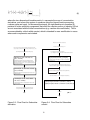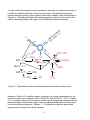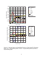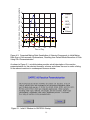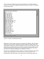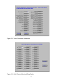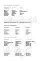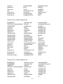
1
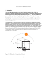
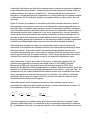
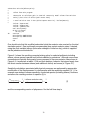
ENVAIR 05-001 February 2005 User’s Guide to URAC Calculations Kenneth M. Busness KB Consulting, Kennewick, Washington Jeremy M. Hales Envair, Pasco, Washington Prepared for Argonne National Laboratory under Contract No. 2F-00871 by Envair 12507 Eagle Reach Pasco, Washington 99301 DISCLAIMER This report was prepared as an account of work sponsored by an agency of the United States Government. Neither the United States Government nor any agency thereof, nor Argonne National Laboratory, nor Envair, nor any of their employees or subcontractors makes any warranty, expressed or implied, or assumes any legal liability for the accuracy, completeness, or usefulness of any information, apparatus, product, or process disclosed, or represents that its use would not infringe privately owned rights. Reference herein to any specific commercial product, process, or service by trade name, trademark, manufacturer, or otherwise, does not necessarily constitute or imply its endorsement, recommendation, or favoring by the United States Government or any agency thereof, or Argonne National Laboratory, or Envair. The views and opinions of authors expressed herein do not necessarily state or reflect those of the United States Government or any agency thereof. ENVAIR for the UNITED STATES DEPARTMENT OF ENERGY under ANL Contract No. 2F-00871 ENVAIR 05-001 February 2005 User’s Guide to URAC Calculations Kenneth M. Busness* Jeremy M. Hales Prepared for Argonne National Laboratory and the U.S. Department of Energy under Contract No. 2F-00871 Envair Pasco, Washington 99301 *KB Consulting, Kennewick, Washington Blank Page Abstract The User’s Reactivity Analysis Code (URAC) is computation facility which allows a user, with minimum effort or knowledge of atmospheric chemistry and computation techniques, to simulate and display atmospheric-chemistry interactions on desktop and laptop computers. It is based on a simple box-model approach, and is designed primarily for two user communities: 1. Persons wishing to increase their understanding of tropospheric chemistry in a straightforward and convenient manner, without the burden of acquiring prior knowledge of the computational basis. A primary target audience for this application consists of collegelevel students of atmospheric chemistry; but it should useful as an instructional tool to a variety of other interested persons as well. 2. Persons involved with policy analysis and air-quality management decision processes. While the limitations of code’s box-model approach are obvious, it is nevertheless valuable as a scoping tool for evaluating alternative control scenarios prior to selection, implementation, and/or more detailed modeling analysis. The current computational system accommodates three different reaction parameterizations: Carbon Bond 4, SAPRC-90, and SAPRC-97. These parameterizations were prepared elsewhere, and were processed for use in URAC using software provided by the Flexible Chemical Mechanism system developed by Kumar and his coworkers. In addition to computing time-series of pollutant concentrations the code performs sensitivity calculations, which can be used for interpreting reaction behavior and component dependencies as well as for computing reactivity scales of arbitrary definition. Codes presented in this report are intended for Unix systems, and were prepared using Macintosh and Sun platforms. They can be operated in a simple batch mode or through the use of an X-Windows-based graphical user interface. CONTENTS Section Page 1. Introduction……………………………………………………………….. 1 2. Governing Equations……………………………………………………. 3 3. Code Description………………………………………………………... 3.1 Overview……………………………………………………………. 3.2 Code Initialization………………………………………………….. 3.3 Main Computation Loop…………………………………………... 4 4 4 7 4. Basic Code Operation and Interpretation: Batch Mode………………………………………………………………. 11 Basic Code Operation and Interpretation: GUI Mode…………………………………………………………………. 17 6. Advanced Operations………………………………………………….. 25 7. Future Extensions………………………………………………………. 28 References………………………………………………………………………. 30 5. Appendix A: Software Installation Instructions………………………….. A-1 Appendix B: Description of Source Code Files………………………….. B-1 LIST OF ILLUSTRATIONS Figure Page 1.1 Schematic of Computational Domain ……………………………… 1 3.1 Flow Chart for Code Initialization …………………………………… 6 3.2 Flow Chart for Main Computation Loop ……………………………. 8 3.3 Flow Chart for Subroutine derivative ……………………………….. 10 3.4 Flow Chart for Subroutine sensint …………………………………... 10 4.1 Simplified Schematic of Interacting Reaction-Chemistry Components ……………………………………………………………… 12 4.2 Selected Output from Default-Mode Execution of Code ………… 18 4.3 Computed Mixing-Ratio Sensitivities of Selected Compounds to Initial Mixing Ratio Sum of Non-aromatic Hydrocarbons ……….. 19 5.1 Initial X Window for SAPRC90 Startup ……………………………… 19 5.2 Reaction Parameterization Listing …………………………………… 20 5.3 Control Parameter Initialization ………………………………………. 21 5.4 Initial Chemical Species Concentrations …………………………… 21 5.5 Species for Plotting …………………………………………………….. 22 5.6 Sensitivity Species ……………………………………………………… 23 5.7 Plotted Results for Species Mixing Ratios …………………………. 24 5.8 Plotted Sensitivities to Initial NO Mixing Ratio …………………….. 24 6.1 Selected Computed Mixing Ratios from Default-Mode Execution of Code Augmented by Ethene and Higher Olefin Emissions …… 27 6.2 Computed Mixing-Ratio Sensitivities of Selected Compounds to Ethene Emissions, Resulting From Code Execution Under the Conditions of Figure 4.4 …………………………………………… 28 LIST OF TABLES Table Page 1.1 Parameters Read by Subroutine cntrlprm …………………………. 5 4.1 CB-4 Parameter List ……………………………………………………. 13 4.2 SAPRC-90 Parameter List ……………………………………………... 14 4.3 SAPRC-97 Parameter List ……………………………………………... 15 User’s Guide to URAC Calculations 1. Introduction This report describes operation of the User’s Reactivity Analysis Code (URAC), a tropospheric-chemistry calculation facility, which is based on a box-model description of the pollutant-containing air parcel shown schematically in Figure 1.1. The box’s contents are presumed to be well mixed and subjected to solar insolation, which varies with geographical location, date, and time of day. Based on this conceptual framework, the code simulates chemical reaction, inflow, outflow, emissions, deposition, and ventilation, calculating chemical-species concentrations and associated sensitivity coefficients as functions of elapsed time. The original intent of this project was to render the computational framework sufficiently adaptable to accommodate a variety of chemical parameterization schemes. While this is indeed the case in principal, the current software allows chemical conversion within the parcel to be simulated using three chemistry parameterizations only: CB-4, SAPRC-90 and SAPRC-97. Adaptation of these schemes for this code was performed using the Flexible Chemical Mechanism (FCM) software produced by Kumar, Lurmann, and Carter (1995). This procedure, as well as required steps for adaptation of additional schemes, is discussed later in this report. aloft ci in ci ∆z c i r i w i ∆y di ∆x q i Figure 1.1: Schematic of Computational Domain 1 The software associated with this code is written for Unix operating systems and allows execution in batch mode as well as through a graphical user interface (GUI). As such it provides a convenient facility for executing the reaction codes, which requires little prior knowledge of atmospheric chemistry or the intricacies of formulating and solving the associated equations. These features reflect the primary intent of this software, which is to serve the following two groups of users: 1. Persons wishing to increase their understanding of tropospheric chemistry in a straightforward and convenient manner, without the burden of acquiring prior knowledge of the computational basis. A primary target audience for this application consists of collegelevel students of atmospheric chemistry; but it should useful as an instructional tool to a variety of other interested persons as well. 2. Persons involved with policy analysis and air-quality management decision processes. While the limitations of this simple box-model approach are obvious, it is nevertheless valuable as a scoping tool for evaluating alternative control scenarios prior to selection, implementation, and/or more detailed modeling analysis. One particular application of this code is its use as a tool for calculating reactivities of airpollution constituents, and at the outset it is important to note that a diversity of definitions of the term “reactivity” is applied throughout the published literature. As an example, Carter (1995) defines “maximum incremental reactivity” (MIR) of species j as ( ∂[O3 ] )x , x ...x , x ≠ x j ∂x j 1 2 n where [O3] is the calculated ozone concentration at the time of its diurnal maximum and xj is the amount of a specific precursor, j, admitted to the system through its initial and boundary conditions. This definition is further constrained by selecting the concurrently existing NO x abundance to maximize the peak ozone reactivity, when calculated characterizing xj as the concentration of the concurrently existing volatile organic compound (VOC) mix. Quite obviously a profusion of other reactivity definitions can be, and have been, posed. Even if one accepts the definition given above as a standard, it is obvious that a wide range of associated numerical values can arise depending on which reaction parameterization is employed, what VOC mix is chosen, and what environmental conditions of solar insolation, humidity, temperature, dilution, and so-forth are imposed. 2 Jump Start: • For systems with this software installed, one can execute the code immediately as follows: 1. Open a Unix terminal X Window and change to the directory containing the GUI code version. 2. Type the command ./startmodel This will initiate execution for the basic model system via the graphical user interface. • To install software, see Appendix A. The computational procedure described in this report takes a neutral approach to this issue by providing a versatile platform, which enables the user to stipulate whichever reactivity definition he or she prefers. In essence the code computes “sensitivity coefficients,” ∂c si, j (t) = i ∂α j α k ≠ α j , (1) where ci is the concentration of species i and αj the parameter selected for the sensitivity test (e.g., initial abundance of precursor j, solar insolation, a specific reaction-rate coefficient, deposition flux, . . ). Given this the user may select conditions appropriate to MIR or an alternate reactivity definition of choice, execute the code, and obtain the desired result. The following sections of this report instruct the potential user on procedures for applying the code to this end. 2. Governing Equations The governing equations associated with this code are ∂ci uciin uci (cialoft − ci ) d(∆z) qi w i di = − + + − − +r ∆x ∆ x ∆z ∆z ∆ z ∆ z i ∂t dt (2) where t = the independent variable, time u = the advection velocity, m/s ci = the concentration of component i in the volume element, moles/m3 cini = the concentration of component i entering the volume element, moles/m3 cialoft = the concentration of component i immediately above the volume element. moles/m3 qi = the emission flux of component i, moles/(m2 hr) wi = the wet-deposition flux of component i, moles/(m2 hr) di = the dry-deposition flux of component i, moles/(m2 hr) ri = the chemical production rate of component i, moles/(m3 hr) ∆x, ∆y, ∆z = dimensions of the model box in the x, y, and z directions, respectively, m 3 The corresponding sensitivity equations are ∂c aloft d( ∆z) c c ∂ − [( ) ] ∂ i in i i s ∂ i, j 1 ∂(uci ) 1 ∂(uci ) 1 dt t ∂ = + − = ∂α j ∂t α j ∆x ∂α j ∆x ∂α j ∆z ∂α j t t t + (3) ∂r 1 ∂qi ∂w i ∂di − ( − )t + i ∆z ∂α j ∂α j ∂α j ∂α j t where si,j = the change in the dependent variable, ci, induced by a change in the parameter αj; i.e., the “sensitivity” of ci to αj. αj = the parameter being subjected to the sensitivity test. The partial derivatives on the right-hand side of (3) imply that t is constrained, but do not ∂ri impose constraints on ci or other parameters in the equations. In particular, ∂α is jt calculated in the code in terms of its constrained counterparts, as ∂ri ∂ri ∂ri ∂α = ( ∂α )t;α ≠ α j ; c1, c 2 , ... + ∑ sk,j ( ∂c )t,c ≠ c k ;α 1,α 2 , ... jt all k j k (4) 3. Code Description 3.1 Overview Appendix B provides the Fortran and C source codes for the calculation system. The code’s algorithms approximate solutions to equations (2) and (3) using the method of fractional steps, which separates the reaction-related terms from their non-reaction counterparts over short time-intervals of length dt (hours), integrates these terms individually, and then recombines the results to compute dependent-variable values at the intervals’ ends. The time variable t (hours) is incremented at each step, and the process continues until it exceeds the pre-set variable tstop (hours), whereupon a normal exit occurs. Instructions for executing this code in both GUI and batch modes are given in Section 4. 3.2 Code Initialization Figure 3.1 is a schematic for initializing batch-mode operation of the basic code. GUIbased operation is similar except for provisions for interactive input and online plotting. As indicated by this schematic, primary control of the code’s execution occurs in the main 4 program main through sequential interrogation of a number of subroutines. The first of these, cntrlprm, reads data from the user-supplied simcontrol file to establish several basic geographic and control variables, including position, start and stop dates and times, print controls, the bypass toggles istatic and isens, and various control parameters for the ordinary differential-equation solver, (Table 1.1). Subsequent to this the main program interrogates subroutine timespan, which calculates the simulation time in hours, from the start and stop times and dates read in through cntrlprm. Next in the calling sequence is subroutine chread, which was taken directly from the FCM code and modified only slightly for present use. This subroutine reads the FCM-generated CHEMPARM file to obtain chemical species names and associated chemical-reaction rate parameters. Within this process the code establishes lookup tables of photolysis coefficients as functions of solar zenith angle [phorate(angle, species)], which will be interpolated to determine photolysis rates as functions of time later in the code. This is followed by interrogation of (user-supplied) subroutine init, which sets initial conditions for the chemical species’ mixing ratios (parts per million), which are placed in the onedimensional array, c. The code allows sensitivity calculations to be performed or bypassed at the user’s discretion, by setting the control toggle isens to 1 or 0, respectively. Under conditions when isens = 1, the main program calls subroutine initsens to supply initial conditions for the sensitivity equations [equations (3), above]. Table 1.1 Parameters Read by Subroutine cntrlprm mrunid run title iprint(1) printing interval istatic control variable: = 1 for non-variable meteorology; 0 otherwise isens control variable: sensitivity calculations done if = 1 lat latitude, degrees long longitude, degrees iy year im month id day tz time zone nbd begin day (day of start month) ned end day (day of end month) tbeg begin time (hrs since mindnight of start day) tend end time (hrs since midnight of stop day) nsteps max. steps in integration dtmin smallest time increment (hr) tslin max time increment (hr) relerr relative error abserr absolute error frdark dark criterion alowlmt lower limit for species concentrations 5 6 cntrlprm f Sets internal species indices kint(i) specid Figure 3.1: Flow Chart for Code Initialization Set element volume (deltax, deltay, deltaz; m), major time increment (dt, hr), and internal clock variables (t; hr, taftrmn;min) Initializes sensitivity coefficients [sens(i)]. initsens(sens) t Sensitivity calculations desired (isens = 1)? Sets initial mixing ratios (ppm) in array c. initialize(c) Sets basic reaction parameters and species count, byreading the CHEMPARM file (unit 9) chread Computes run time in hours (tstop) from start and stop dates. timespan Reads basic control parameters: run title, start & stop dates, ode solver control parameters, toggle for sensitivity calculations. Reads data from simcontrol file (unit 8). Start Converts mixing ratios to concentrations (moles/m**3). concmxratio (1, nsmax, tempdegk, php, c) Prints initial conditions print(t, c, sens) Steady-states ozone, nitrous acid, and possibly other dependent variables steady(lssic, c, lerror) Prints initial conditions print(t, c, sens) Computes thermal raqte coefficients, coeff(i) newrk Computes photolysis coefficients, coeff(i) newphk Computes temperature (tempdefk; K) and pressure (php; hPa) at time tbeg; h. temperature(tbeg, tempdegk, php) Proceed to main computation loop Computes concentration change rate in volume contributed by emission input; emiss (moles/(m**3h) emission(deltaz, emiss) Computes concentration change rate in volume contributed by advective input advin (moles/(m**3h) advectinput(u, deltax, advin) Computes wind speed, u (m/h) wind(u, t) Comnputes solar angle from horizon (degrees) solarz(sla, slon, tz, iy, im, id, time, d,nv) Upon setting the element dimensions and time increment, and initializing the run clock, the code interrogates subroutine temperature to compute the local temperature and pressure. It then calls subroutine newphk to determine, for the current time and location, rate coefficients for all photolysis reactions. newphrk in turn calls subroutine solarz to determine the solar angle at the current time and location. This is used in turn in conjunction with the photolysis look-up tables to determine photolysis rate coefficients coef(i) for each photolytic species i. Subsequent to setting rate coefficients for all photolysis reactions, the program proceeds to interrogate subroutine newrk to determine rate coefficients rk(i) for the system’s thermal reactions. The code then performs initial steady-state calculations as dictated by the specific reaction parameterization in use and proceeds to print the system’s initial conditions to the file AAoutput. Subroutine print, used for this purpose, is user-supplied and should be modified for use with different chemical mechanisms as appropriate for the constituents contained in these parameterizations. The above operations complete initialization required for chemical-reaction calculations. These are followed immediately by initial operations for non-reaction processes within the model volume deltax, deltay, deltaz, including emission and advection. The first step in these operations is to convert all chemical mixing ratios to their concentration equivalents in units of gram-moles per cubic meter, using subroutine concmxratio, followed by interrogation of subroutines advectinput and emission to determine associated contributions to the rates of change in pollutant concentration within the model volume. This information is stored in units of gram-moles per cubic meter hour in arrays emiss(i) and advin(i), for emission and advection, respectively. This concludes program initialization. 3.3 Main Computation Loop Figure 3.2 shows the sequence of the code’s main computation loop. Upon completing initialization operations the code updates the wind, temperature, emissions, and inflow boundary conditions as required, followed by updates for concentration-change rates associated with advective output, wet and/or dry deposition, and entrainment of air from aloft. These steps are followed immediately by integration of the physical-process contributions to the concentration variables for one-half time-step. If sensitivity calculations are desired, the code then interrogates subroutine physsens to provide a similar integration for the chosen sensitivity parameters. Subsequently the concentrations are converted back into mixing ratios, and photolysis and thermal reactionrate coefficients are updated in preparation for chemical-reaction computations, which are coordinated through the numerical integration scheme slsodec. slsodec is a standard Gear integration package, modified to store historical concentration values for subsequent use in the sensitivity-coefficient integration. In contrast to the half time-step integrations described above for the physical processes, one call to subroutine slsodec results in chemical integrations over a full time-step, dt. Subsequent to completion of integration for the current time step the code proceeds to check for, and perform simplified operations for nighttime chemistry, and also calculates total odd-nitrogen abundance for later use in material-balance adjustments. 7 8 wind(u, t) t Stores lsode variables for use in subsequent calls ssrcom(rsav,isav,1) Computes concentration change by reaction for time-step dt lsode Computes thermal raqte coefficients, coeff(i) newrk Computes photolysis coefficients, coeff(i) newphk Converts concentrations to mixing ratios (ppm) concmxratio (2, nfast, tempdegk, php, c) taftrmn = t*60 +tbeg*60 Advances sensitivity calculations for physical processes physsens(advin,advout,emiss, dep,entr,c,sens,nospec, deltax,deltaz,dt) f Sensitivity calculations required (isens=1)? c(l) = c(l)+(advin(l)+advout(l)+emiss(l)-dep(l)+entr(l))+ *.5*dt Figure 3.2: Flow Chart for Main Computation Loop Computes concentration change rate in volume contributed by entrainment entr (moles/(m3h) entrain(deltaz, entr) Computes concentration change rate in volume contributed by deposition dep (moles/(m3h) deposition(deltaz,dep) Computes concentration change rate in volume contributed by advective output advout (moles/(m3h) advectoutput(c, u, deltax, advout) Computes concentration change rate in volume contributed by emission input; emiss (moles/(m**3h) emission(deltaz, emiss) Computes concentration change rate in volume contributed by advective input advin (moles/(m3h) advectinput(u, deltax, advin) Computes temperature (tempr; K) and pressure (php; hPa) at time t; h. temperature(t, tempr, php) Computes wind speed, u (m/h) f Are temperature, wind-speed, emissions, and boundary conditions time-invariant (istatic = 1)? t Continue from initialization sequence (Figure 3.1) t wind(u, t) f Computes concentration change rate in volume contributed by advective input advin (moles/(m3h) advectinput(u, deltax, advin) Computes temperature (tempr; K) and pressure (php; hPa) at time tbeg; h. temperature(tbeg, tempr, php) Computes wind speed, u (m/h) t t = t + .5*dt Are temperature, wind-speed, emissions, and boundary conditions time-invariant (istatic = 1)? tin = tout Computes sensitivity-coefficient change associated with reaction for time step dt sensint(sens) Reset time: tin = tin -60*dt f Sensitivity calculations required (isens=1)? Converts mixing ratios to concentrations (moles/m**3) concmxratio (1, nsmax, tempr, php, c) t f Time limit exceeded (t > tstop)? t Stop Output results as dictated by print-control variable iprint(1) Advances sensitivity calculations for physical processes physsens(advin,advout,emiss, dep,entrain,c,sens,nospec, deltax,deltaz,dt) f Sensitivity calculations required (isens=1)? c(l) = c(l)+(advin(l)+advout(l)+emiss(l)-dep(l)+entr(l))+ *.5*dt t = t + .5*dt Computes concentration change rate in volume contributed by entrainment entr (moles/(m3h) entrain(deltaz, entr) Computes concentration change rate in volume contributed by deposition dep (moles/(m3h) deposition(deltaz,dep) Computes concentration change rate in volume contributed by advective output advout (moles/(m3h) advectoutput(c, u, deltax, advout) Computes concentration change rate in volume contributed by emission input; emiss (moles/(m**3h) emission(deltaz, emiss) If sensitivity calculations are desired the code performs a numerical integration of equation (4) by calling subroutine sensint. sensint uses a fully implicit numerical scheme, which is made possible by the linearity of equation (4). Subsequently the code performs an integration of the physical-process components for a second half-step in a manner identical to that used for the first half-step, updates all computed values and proceeds to the next time step. Figure 3.3 shows a progression of subroutine calls within subroutine derivative, which is interrogated at various points by slsodec and its subservient routines prepj and stode, as well as by fdjac, a Jacobian matrix generator used in the sensitivity-coefficient integration. Upon successful execution derivative returns the chemical transformation rates for each of the chemical species (units of ppm/min, in the vector argument a4). As such, derivative serves as the main portal between the chemical mechanism and the remaining code. All attempts to expand this software to include additional chemistry parameterizations must begin by making appropriate modifications to this subroutine and its subsidiary subroutines, as well as providing suitable replacements for the subroutines newphk and newrk. Subroutine rates accepts information on concentrations and chemical-reaction rate coefficients, and calculates the individual reaction rate of each species pertaining to each individual reaction. Subroutines chmfst and chmslo accept individual-reaction rate information generated by rates, and proceed to compute collective reaction rates for each species by summing over all relevant reactions. These values are returned to the calling routine via the vector a4 and applied as input to the numerical integration process. Subroutines rates, chmslo, and chmfst in the version of derivative supplied with this software were prepared by executing a modified version of the Flexible Chemical Mechanism (FCM) code, and contain some artifacts associated with FCM. Most importantly, the published FCM package applies an ordinary differential-equation solver that depends on the chemical species being segregated into two classes: “slow” and “fast.” As noted previously, the code included with the present system uses a modified Gear solver, where segregation into slow and fast species is not required. The coding in subroutine derivative controls input and output to and from chmslo and chmfst in a manner that is compatible with the Gear-based integrator. Subroutine sensint, which integrates that portion of the sensitivity equation that is associated with chemical-transformation-processes, is shown schematically in Figure 3.5. From equations (3) and (4) this can be written as chem ∂si,j ∂t α j ∂r ∂r = i = i ∂α j t ∂α j t,α ≠α ,c j 1 ,c 2 ∂r + ∑ i all k ∂ck t,c ≠c ,.. . (5) k ,α 1 ,α 2 ,.. Upon interrogation by its calling routine, subroutine sensint activates a Jacobian matrix generator (subroutine fdjac) to compute the array of concentration derivatives in equation (5). Subsequent to this step it sets up the matrices for the implicit finite-difference equation 9 [s ] = [s ] + δt[J ][s ] t +δt i t i i,k t +δt k ∂ri + ∂α j , α ≠ α t , , c , c ,.. j 1 2 (6) where the two-dimensional Jacobian matrix Ji,k represents the array of concentration derivatives, and solves this system of equations using the Linpack matrix-processing routines sgefa and sgesl. As discussed previously, the right-hand term in equation (6) pertains to active sensitivity components that affect the reaction portion of equation (3) but are not associated with the initial concentrations (e.g. reaction-rate coefficients). This is accommodated by a block within sensint, which is intended for user modification in cases where such components are included. Entry from call to subroutine sensint(sens) Set index of historical time-step: n = 1 Entry from call to internal function f (derivative) from subroutine slsodec, prepj, and stode, as well sa from subroutine fdjac (derivative (neq, t, y, a4)) rdt = reciprocal of historical time increment y(n) = average of end-point mixing ratios for historical time increment Store mixing-ratio arrays in a0 and a5 working arrays rates(a0, rk, a2, coef, a4, a5, cst, t, nsmax) fdjac(nsmax,nsmax,y,concjac) Computes jacobian: derivatives of rxn rate wrt concentration at historical step n . Calculates "throughput rates" for the individual reactionspecies combinations. For example the thoughput rate for species A the reaction A + B → C + D equals the production rate of A by this reaction Do the sensitivity calculatios associated with reaction processes include any sensitivity paramenters other than initial concentrations? f t chmslo(a0, rk, a2, coef, a4, a5, cst, t, nsmax) Compute associated partial derivatives (as user-supplied block) Applies throughput rates to compute reaction rates for each chemical species. Load matrix elements for numerical integration of equation (4) chmfst(a0, rk, a2, coef, ahold, a5, cst, t, nsmax) Solve matrix equation to obtain implicit numerical integration of equation (4): sgefa(concjac,nsmax+1,nsmax+1,indx,d) sgesl(concjac,nsmax+1,nsmax+1,indx,sens,0) Applies throughput rates to compute reaction rates for each chemical species. Move ahold array contents into high side of a4 array: a4 array now holds updated reaction rates, ppm/min. n > isteps? Return Return n = n +1 Figure 3.3: Flow Chart for Subroutine derivative Figure 3.4: Flow Chart for Subroutine sensint 10 Completion of the reaction-chemistry block in the main program results in an integration of chemical processes and associated sensitivity coefficients for one time-step. The program (Figure 3.2) subsequently converts all mixing ratios to concentrations and embarks on a half time-step integration for physical processes in a manner identical to that shown on the left-hand side of the diagram, completing a full integration of all processes over a time-step dt. Finally the code outputs the results to file or to the GUI as required. Provided the desired time-limit has not been exceeded, the program loops back to perform operations for the subsequent time-step. Otherwise the program performs a normal termination. Depending on whether the batch-mode or GUI versions are used, the code outputs computed variables on an hourly basis as dictated by the user interface or by the user-modifiable subroutine print. In both cases the code writes selected output to the diagnostic file tracefile, which is intended for debugging purposes in the event of failed execution. 4. Basic Code Operation and Interpretation: Batch Mode As noted in the previous section the current code version allows the choice between three different chemical parameterization schemes, as implemented through the Flexible Chemical Mechanism (FCM) preprocessing code. FCM is documented in a report by Kumar, et al (1995), and the associated software is available on the Internet (www.arb.ca.gov/eos/research/research.htm). Documentation for the three chemistry parameterization schemes is given as follows: CB-IV SAPRC-90 SAPRC-97 Gery, et al. (1989)1 Carter (1990) Carter, et al. (1997) Because this documentation exists, this report will not provide a detailed discussion of these parameterizations or of the FCM preprocessor, other than to note some FCM adaptations necessary for present purposes2. The most important of these adaptations reflects the fact that the FCM was prepared mainly to interface the chemical schemes with the three-dimensional SAI Urban Airshed Model, UAM-4. Partly as a consequence of this fact, the present code has made liberal use of a few UAM-4 subroutines, notably those involving nighttime chemistry and solar insolation. In addition, this software applies a modified version of the Gear ordinary-differential equation solver published by Hindmarsh (1983) as well some Linpack matrix processing routines included with the Gear code distribution. The origins of these incorporated codes are indicated by comment statements in the associated subroutines. 1 Several variants of the basic CB-4 scheme are in current use. The version employed here is that supplied with the FCM preprocessor software. 2 Numerous small modifications to the published FCM code were necessary to enable operation on the Sun and MacIntosh operating systems. 11 For users with limited experience with tropospheric chemistry it is useful at the outset to consider a simplified schematic chemical representation, indicating the interactions between nitrogen species, organic species, and various oxidants, such as that shown in Figure 4.1. Consulting this figure when viewing graphical output from the code is often useful in facilitating insights with regard to the interacting chemical processes. O2 HO ole HO2 s O3 hν hν O2 PAN, PPN, . . . 2 NO O O1D H 2O HNO2 O3P HO + O3 NO ±R hν RO , HO fin ts, c u od H 2O r p , c i 2 an , CO g or CO NO2 HO2, RO2 RO2, HO2 O3 NO3 HO2 HO VOC HO2NO2 HO hν RHO2, H2O2 ±HO2 HNO3 ±NO2 O2 H + CO2 HO N2O5 CO Figure 4.1: Simplified Schematic of Interacting Reaction-Chemistry Components Because of Figure 4.1’s simplified nature, it provides only a loose representation of the chemical components contained in CB-4, SAPRC-90, and SAPRC-97. “VOC” in Figure 4.1, for example, represents the totality of volatile organic compounds, whereas the three parameterization schemes treat some of these compounds individually and lump others into several different categories. Tables 4.1 – 4.3 indicate the chemical species and species groups included in the three schemes. 12 Table 4.1. CB-4 Parameter List Index Chemical Species or Lumped ParameterName Default Initial Condition, ppm h2o o3 no no2 no3 n2o5 c2o3 xo2 pna cro hno3 hono pan h2o2 par eth ole tol xyl isop meoh co form ald2 cres mgly open etoh ntr ho2 ror water ozone nitric oxide nitrogen dioxide nitrate radical dinitrogen pentoxide peroxy acyl radical lumped peroxy radicals oxidizing NO to NO2 higher peroxyacyl nitrates cresol oxidation intermediate nitric acid nitrous acid peroxy acetyl nitrate‘ hydrogen peroxide parafins (alkanes) ethene olefins (alkenes) toluene xylene isoprene methanol carbon monoxide formaldehyde higher aldehydes cresol methyl glyoxal open ethanol organic nitrates hydroperoxy radical ethers 20000. 0.0 0.045 0.005 0.0 0.0 0.0 0.0 0.0 0.0 0.0 0.0 0.0 0.0 0.6 0.025 0.025 0.0214286 0.0125 0.0005 0.0 1.0 0.025 0.0125 0.0 0.0 0.0 0.0 0.0 0.0 0.0 13 Table 4.2 SAPRC-90 Parameter List Index Chemical Species or Lumped Parameter Name Default Initial Condition, ppm h2o o3 no no2 no3 n2o5 hno3 hono hno4 ho2 co ho2h ro2 ooh cco3 c2co3 pan ppn hcho ccho rcho mek rno3 cres mgly afg2 so2 ethe ole1 ole2 ole3 ole4 alk1 alk2 aro1 aro2 sulf hcooh ccooh aux1 aux2 water ozone nitric oxide nitrogen dioxide nitrate radicals dinitrogen pentoxide nitric acid nitrous acid peroxynitric acid hydroperoxy radical carbon monoxide hydrogen peroxide alkyperoxy radical total hydroperoxide groups acetyl peroxy radicals higher acylperoxy radicals peroxyacetyl nitrate higher peroxyacyl nitrates formaldehyde acetaldehyde higher aldehydes ketones and higher oxygenated products organic nitrates cresols, phenols, and other aromatic oxygenates methyl glyoxal and other alpha-dicarbonyls uncharacterized fragmentation products sulfur dioxide ethene other terminal alkenes internal alkenes isoprene terpenes less reactive alkanes more reactive alkanes monoalkyl benzenes more reactive aromatics sulfate formic acid acetic acid auxiliary species 1 (reacts only with OH) auxiliary species 2 (reacts with OH, O3, O, NO3, and hv) 20000. 0.0 0.045 0.005 0.0 0.0 0.0 0.0 0.0 0.0 1.0 0.0 0.0 0.0 0.0 0.0 0.0 0.0 0.025 0.00375 0.0016625 0.0015 0.0 0.0 0.0 0.0 0.0 0.025 0.0125 0.0025955 0.0035 0.00075 0.0675568 0.0374675 0.0214286 0.0125 0.0 0.0 0.0 0.0 14 0.0 Table 4.3 SAPRC-97 Parameter List Index Chemical Species or Lumped Parameter Name Default Initial Condition, ppm h2o o3 no no2 n2o5 n2o5 no3 ho2 ro2 rco3 hno3 hono hno4 pan ppn nphe gpan pbzn co co2 h2o2 xooh hcho ccho rcho acet mek rno3 gly mgly phen cres bald afg1 afg2 ethe h2 xc xn ch4 alk1 water ozone nitric oxide nitrogen dioxide dinitrogen pentoxide dinitrogen pentoxide nitrate radicals hydroperoxy radical total organic peroxy radicals total acyl peroxy radicals nitric acid nitrous acid peroxynitric acid peroxyacetyl nitrate higher peroxyacyl nitrates nitrophenols PAN analog formed from glyoxal PAN analogs formed from aromatc aldehydes carbon monoxide carbon dioxide hydrogen peroxide total hydroperoxide groups formaldehyde acetaldehyde higher aldehydes acetone ketones and higher oxygenated products organic nitrates glyoxal methyl glyoxal and other alpha-dicarbonyls phenols cresols and other aromatic oxygenates benzaldehyde uncharacterized fragmentation products uncharacterized fragmentation products ethene hydrogen lost carbon lost nitrogen methane less reactive alkanes 20000. 0.0 0.045 0.005 0.0 0.0 0.0 0.0 0.0 15 0.0 0.0 0.0 0.0 0.0 0.0 0.0 0.0 1.0 0.0 0.0 0.0 0.025 0.00375 0.0016625 0.0 0.0015 0.0 0.0 0.0 0.0 0.0 0.0 0.0 0.0 0.025 0.0 0.0 0.0 1.79 0.0675568 Table 4.3 SAPRC-97 Parameter List, Continued Index Chemical Species or Lumped Parameter Name Default Initial Condition, ppm alk2 aro1 aro2 ole1 ole2 ole3 hcooh ccooh etoh mtbe mbut cxo2 tbuo prod inert hc2h rc2h ispd isop bhcho2 c303 hc204 more reactive alkanes monoalkyl benzenes more reactive aromatics other terminal alkenes internal alkenes terpenes formic acid acetic acid ethanol methyl tertiary-butyl ether methyl butenol mtbe reaction product mtbe reaction product mtbe reaction product mtbe reaction product methyl butenol reaction product methyl butenol reaction product lumped isoprene reaction products isoprene lumped isoprene and ispd reaction products lumped isoprene and ispd reaction products lumped reaction product 0.0374675 0.0214286 0.0125 0.0125 0.0025955 0.0035 0.0 0.0 0.0 0.0 0.0 0.0 0.0 0.0 0.0 0.0 0.0 0.0 0.0 0.0 0.0 0.0 These schemes compute a number of additional species, notably several of the radicals shown in Figure 4.1, as steady states. Within the FCM-based representation these steady states are computed explicitly within subroutines chmslo and chmfst. These are not normally output as computed results; however, they can be channeled to output by appropriate modification of these subroutines. Programs associated with the batch-mode code version are contained in the directory Batch_Codes.dir, within the subdirectories cb4.dir, saprc90.dir, saprc97.dir, and com.dir. com.dir contains the source code used by all three mechanisms, while the remaining directories contain mechanism-specific code as well as common files. Default-mode batch execution for any one of the three mechanisms is accomplished by entering the directory for the chosen mechanism, executing the sf macro (by typing ./sf) to create the executable code, and then typing ./program. The code execution resulting from this process writes computed results to the file AAoutput. These default calculations correspond to a location of 47.5N, 122.3W, beginning at 6:00 on July 3, 1998, with the initial mixing ratios shown in Tables 4.1 – 4.3. Simulations for other times, locations, and initial mixing ratios can be performed by making appropriate changes to the files simcontrol, init.f, and initsens.f, and then recompiling with the ./sf command. 16 Figure 4.2 shows plots of mixing ratios and sensitivity coefficients (obtained from the AAoutput file) of selected pollutants corresponding to the default conditions and the CB-4 parameterization. The mixing ratios indicate typical behavior of photochemical ozone production with simultaneous reduction of NO and ethene, plus the buildup of reaction products such as nitric acid and PAN. The lower plot shows the sensitivity of these same species to initial NO mixing ratio. Ozone exhibits a negative sensitivity to initial NO in the first few hours, owing to nitric-oxide titration of ozone and ozone-producing radicals. As expected the sensitivity of NO to its own initial condition is initially unity. Sensitivity coefficients can be computed for the initial conditions of multiple species. For example, if one wishes to compute sensitivities to the total non-aromatic hydrocarbon mix (par + eth + ole + isop in the CB-4 parameterization), one could simply set the corresponding initial sensitivity coefficients to unity in file sensinit.f. Figure 4.5 shows selected output resulting from this action. As can be noted from this figure, ozone sensitivities show a rapid initial rise with a subsequent falloff resulting from competing effects of hydrocarbon reaction products. 5. Basic Code Operation and Interpretation: GUI Mode Graphical user interface (GUI) operation is the simplest way to execute the code. One simply moves to the directory containing the code for a specific reaction parameterization and, if compilation to create an executable code is required, types the command ./sf. Once the executable codes for all parameterizations exist, moving to the next highest directory and typing ./startmodel presents the user with a choice of parameterizations and a consecutive series of windows that allow selection of simulation location, date, and time, as well as initial mixing ratios and sensitivity parameters. The GUI also allows execution using default parameters, which are identical to those described above for batch operation. Computed results take the form of plots similar to those shown in Figures 4.2 and 4.3. The user interface to facilitate user access to the Fortran-based chemical-reactivity codes is written in the C programming language and implemented in X Windows. It is generic and independent of the user’s Unix platform, providing the platform contains the requisite X Windows drivers, which are all available for public use, with some limitations. The application makes extensive use of XForms1, a powerful graphical user interface toolkit for X Windows. This GUI was developed on Mac OSX version 10.3 and Sun OS Release 5.8 using X11R6 in a Unix environment. Simplicity of operation through the use of interactive graphics makes execution of the chemical-reactivity calculation codes a very “user-friendly” process. The user is presented with a series of windows relevant to the chemistry parameterization selected (CBIV, SAPRC90, SAPRC97) which enable input of initial environmental conditions, initial chemical species concentrations, and the ability to select groups of species for plotting along with species to be used as sensitivity parameters. 1 Xforms Version 1.0.90 is the Free Software distribution of the Xforms Library. It is licensed under the GNU Lesser General Public License version 2.1. Xforms was developed and copyrighted by T.C. Zhao and Mark Overmars. It is not public domain, but is free to use in non-commercial and not-for-profit purposes. 17 0.05 B Ozone X .1 0.045 J J NO Mixing Ratio, ppm 0.04 H NO2_ 0.035 F HNO3 H 0.03 J H 0.025 0.02 0.015 0.01 0.005 H H B B BF BF BF BF BF BF F BF F J BF H BF J F BF 0B 6 8 10 12 14 Time of Day Sensitivity to Initial NO Mixing Ratio 16 18 B B B B B B B 2 H J B Ozone J NO B 1.5 H NO2_ F HNO3 H H F F F F F F F F J FJ H H F F J HJ HJ HJ HJ HJ HJ HJ F H F 0B B 0.5 Ethene J HJ HJ HJ HJ HJ HJ HJ HJ 2.5 1J J PAN PAN Ethene -0.5 B -1 B B -1.5 6 8 10 12 14 Time of Day 16 18 Figure 4.2: Selected Output from Default-Mode Execution of Code Using CB-4 Parameterization. Top: Computed Mixing Ratios. Bottom: Computed Mixing-Ratio Sensitivities to Initial NO Mixing Ratio. 18 Sensitivity to Combined Olefin + Paraffin Mixing Ratio 6 B Ozone B 5 J NO H NO2_ B 4 F HNO3 3 PAN B 2 B Ethene B B B B B B B 1 H F F FJ FJ HJ HJ HJ HJ H F 0B HJ BF H J HJ HJ H F F F F F F F J J HJ H -1 6 8 10 12 14 Time of Day 16 18 Figure 4.3: Computed Mixing-Ratio Sensitivities of Selected Compounds to Initial Mixing Ratio Sum of Non-aromatic Hydrocarbons, Resulting from Default-Mode Execution of Code Using CB-4 Parameterization. As shown in Figure 5.1, an initial window provides a brief description of the reaction parameterization for the selected chemistry scheme, and allows the user to evoke a listing of the relevant reactions in a subsequent browser window. Figure 5.1. Initial X Window for SAPRC90 Startup. 19 If the user chooses to display the reaction parameterizations for the model mechanism, clicking on the “Listing” button displays a browser window (shown in Figure 5.2) containing those parameterizations. Figure 5.2. Reaction Parameterization Listing. Selecting the “Continue” button causes the next window to be displayed. With this display (Figure 5.3), the user is able to interactively set initial conditions for several control, time, and geographic variables (e.g., latitude, longitude, year, month, day, start/end times). Initial default values are displayed which can be used for testing the model, and which can all be edited and altered via mouse and keyboard. Entries are made by clicking in the chosen text input block, deleting and adding text, and ending with a <return>. Once the user is satisfied with all entries, clicking on “Continue” will initiate the next step by opening a new window (Figure 5.4), which allows entry of initial mixing ratios for all chemical species. With this window, in the same manner as in the previous window, the 20 Figure 5.3. Control Parameter Initialization Figure 5.4. Initial Chemical Species Mixing Ratios 21 user can edit each text block or use the default values for the chemical species, and again, click on “Continue” to proceed to the next step. A plotting routine provides visual representation of the model output results. Figure 5.5 shows the form in which the user, via several clickable buttons, may select chemical species to be plotted over the time period of the model run. In the interest of keeping plots legible, no more than 5 species may be chosen per plot. Following these selections, clicking on “Continue” advances to the next step. Initial parameters were previously selected in the variables entered as initial conditions (Figure 5.3). One of these control variables determines if sensitivity calculations are to be performed. If the sensitivity control variable is set to 1, an additional plot is generated, showing the effects of the sensitivity species on the species chosen for plotting. In this instance, when “Continue” is clicked following selection of the species to be plotted (Figure 5.5), an additional window is displayed to enable user selection of sensitivity species (see Figure 5.6). If the sensitivity control variable was set to 0, this step is not executed. Figure 5.5. Species for Plotting 22 Figure 5.6. Sensitivity Species When all available selections have been completed, all variables are passed to the Fortran reactivity calculation algorithms as described in Section 4. Following execution of the Fortran routines, data are passed back to the GUI C code plotting routine where the computed mixing ratios and sensitivities time-sequenced plots are generated and displayed as in Figures 5.7 and 5.8. As shown in Figure 5.7, the user can select “Done” and terminate the run or “Next Plot”, which causes the sensitivity plot to be displayed. The model run is now completed, and the user can terminate the program by selecting “Done”, or initiate another run by clicking “Next Run” which will activate the control initialization display (Figure 5.3). This action will start another run using the same model mechanism (e.g., SAPRC90). To execute a different model mechanism (SAPRC97 or CBIV), it is necessary to terminate and restart, selecting the desired model scheme. To capture the screen image of the plot, the “xwd” utility, which is part of the X11 distribution, can be used to retain the image in a .xwd file. To save the image, the user opens another X terminal window, navigates to the executing model directory, and executes 23 Figure 5.7. Plotted Results for Species Mixing Ratios Figure 5.8. Plotted Sensitivities to Initial NO Mixing Ratio 24 the command “xwd > filename.xwd.” The cursor will turn into a crosshair. By moving the cursor to the plot window and clicking, one writes the contents of the window to the specified file. To recall the “xwd” file to the screen, one can use the “xwud” utility, which is also part of the X11 distribution. This is done by typing the command “xwud -in filename” while in the appropriate directory. Subsequently, there are several applications which can convert the “xwd” file into postscript, pdf, or some other format that can be printed. One such conversion application is “xwd2ps,” which will convert the .xwd file to PostScript. To perform such a conversion one moves to an X terminal window, navigates to the directory containing the .xwd file and executes the command “xwd2ps filename.xwd>filename.ps.” This file can be printed to a PostScript printer. 6. Advanced Operations Although the graphical user interface allows convenient manipulation of all variables associated with files init.f, initsens.f, and simcontrol, it does itself not accommodate calculations of physical processes such as emission, deposition, advection, and entrainment. In fact, each of these processes is inactive in the code’s default version, resulting, essentially, in a “batch-reactor” simulation. One can activate these additional processes in a straightforward manner, using either the GUI or batch software, by making appropriate changes to the following files and recompiling the code: advectinput.f advectoutput.f deposition.f emission.f entrain.f physsens.f temperature.f wind.f Documentation contained within these files makes modifications for this purpose a reasonably straightforward process, and here we demonstrate this procedure by imposing 2 X 10⁻⁴ moles/m2 emissions of ethene (eth) and higher olefins (ole) within the construct of the CB-4-based model, using the default parameters for initial mixing ratios, time, and location. The modified emission subroutine is given as follows: 25 subroutine emission(deltaz,emiss) c c called from main program c c subroutine to calculate gain in chemical content by model volume from emission c emiss(i) has units of moles/(cubic meter hour) c c = areal emission rate in box (moles/square meter hr) / deltaz(meters) c include ‘chparm.cmd’ include ‘chdata.cmd’ include ‘jmhdata.cmd’ real emiss(nsmax) do 10 i=1,nospec emiss(i)=0. 10 continue emiss(keth)=.0002/deltaz emiss(kole)=.0002/deltaz return end One should note that this modified subroutine holds the emission rate constant for the total simulation period. One could easily accommodate time-variant emission rates, if desired, using the clock variable taftrmn (hours after midnight of initial run day), which is supplied via the jmhdata.cmd include file. Figure 6.1 shows the resulting computed mixing ratios for selected pollutants including ethene, whose general upward trend reflects addition by emissions. Although ozone rises somewhat more quickly during early hours compared to the zero-emission case shown in Figure 4.2, it maximizes at about 11:00 and then declines, behavior that stems largely from the direct reaction between ethene (and additional olefins) and ozone (cf. Figure 4.1). Sensitivity calculations associated with physical processes are performed by appropriate modification of the file physsense.f in conformance with the sensitivity equation (3). If, for example one wishes to assess sensitivity of selected species (including ethene) to ethene emissions the resulting version of equation (3) is 1 ∂ ethene emission rate 1 ∂si,ethene emision = = ∆z ∂ ethene emission rate ∆z ∂t and the corresponding version of physsense.f for the half time-step is 26 (7) subroutine physsens (advin,advout,emiss,dep,entr,c,sens, + deltax,deltaz,dt) c c called from main program c c this subroutine updates those sensitivity coefficients associated with c non-reaction parameters (e.g., emission, deposition, advective terms, c entrainment), and is intended for modification by the user as appropriate. c the operative return variables ar the updated sensitivity coefficients, c sens(i) corresponding to a chosen sensitivity parameter alpha. c c as an example, say our sensitivity parameter, alpha, is a dry-deposition c velocity of species j. referring to the sensitivity equation given in the c user’s manual, the only term directly influenced by this parameter is the c deposition rate of species j, dj. The derivative d dj/d alphaj is unity; c thus the time-derivative of the sensitivity coefficient is 1.0/deltaz. c accordingly c sens(j) = sens(j) +.5*dt*d[function(i)]/d[alpha(j)] c include ‘senscommon.com’ include ‘chdata.cmd’ include ‘chparm.cmd’ include ‘jmhdata.cmd’ real advin(nsmax),advout(nsmax),emiss(nsmax),dep(nsmax), +entr(nsmax),c(nsmax),sens(nsmax) c c user supplied sensitivity-derivative input: c sens(keth)=sens(keth)+0.5*dt/deltaz return end 0.05 B Ozone X .1 0.045 J J NO Mixing Ratio, ppm 0.04 H NO2_ 0.035 H 0.03 J H 0.025 0.02 F HNO3 H 0.015 B B B B B B B BF B F F F F F F F F PAN Ethene B J F H 0.005 H BF J B F J HJ HJ HJ HJ HJ HJ HJ HJ F 0B 0.01 6 8 10 12 14 Time of Day 16 18 Figure 6.1: Selected Computed Mixing Ratios from Default-Mode Execution of Code Augmented by Ethene and Higher Olefin Emissions Using CB-4 Parameterization. 27 Figure 6.2 shows a plot of the computed sensitivities for this case, using the same initial concentrations and ethene emissions that were applied for Figure 6.1. (Also for this calculation, the original file sensinit.f was modified to remove sensitivity calculations for NO initial conditions.) Here the ethene mixing ratios exhibit a monotonic sensitivity to ethene emissions, as should be expected. Ozone shows an early, strong, and positive sensitivity to ethene emissions, which later decays to negative values reflecting exhaustion of the NOx reactant and the influence of the direct ozone-olefin reaction. Sensitivity to Ethene Emission Rate, h/m Upon studying the examples shown in Figures 4.2, 4.3, 6.1, and 6.2 the reader should be well prepared to expand his or her usage of the code to encompass all features. In sodoing we recommend that the user make an archive copy of the original codes for future reference, to help avoid any forgotten subroutine changes in the working versions. We also recommend executing all three code versions in default mode and archiving the results, for possible use as downstream backchecks on code integrity. 0.0016 B Ozone B 0.0014 J NO 0.0012 B 0.001 H NO2_ B B 0.0008 0.0006 0.0004 F HNO3 B PAN B B 0.0002 Ethene X .1 B B HJ FJ FJ FJ H HJ F FJ F HJ H HJ F HJ F HJ F FJ H F HJ BH 0B FJ F B H H -0.0002 B -0.0004 6 8 10 12 14 Time of Day 16 18 Figure 6.2: Computed Mixing-Ratio Sensitivities of Selected Compounds to Ethene Emissions, Resulting From Code Execution Under the Conditions of Figure 4.4 Using CB-4 Parameterization. 7. Future Extensions Given the evolution of new chemical parameterization schemes and the variety of additional schemes in current existence, it is of some interest to question whether (and how) the procedure described here should be extended to include other reaction parameterizations. As noted above, the codes given in this report were developed using the FCM software, which is centered on the idea of a unified approach to a variety of reaction parameterizatons. FCM was particularly useful for implementing the SAPRAC 28 parameterizations, which were developed originally on a DOS/Windows platform, because it provided a means of migrating the associated codes to a Unix environment. FCM’s unified approach is an attractive concept. It suffers, however, from three significant drawbacks. First, considerable effort is required to adapt a reaction parameterization to the FCM framework, and as a result only a few reaction parameterizations exist under this format.1 Second, documentation in the FCM user’s manual is rather obscure and the code has some machine dependencies, making operation of this software a somewhat challenging proposition. Finally, FCM is designed to serve as a set-up facility for operations with the three-dimensional model UAM-4, and so-doing it produces a number of artifacts that are extraneous for other applications. As noted previously several of these artifacts have migrated to the code presented in this report. As a consequence we suggest that a more direct approach, not involving FCM, be applied in adapting future parameterizations to this computational framework. As noted in Section 3, subroutine derivative serves as the main portal between the chemical mechanism and the remaining code, and all attempts to expand this software to include additional chemistry parameterizations must begin by making appropriate modifications to this subroutine and its subsidiary subroutines, as well as providing suitable replacements for the subroutines newphk and newrk. The flow charts given in Section 3 are intended to aid in extension processes of this type. 1 SAPRC99 is an additional parameterization currently included in the FCM package. SAPRC99’s FCM implementation had not attained sufficient maturity at the time of this development effort to be included with the codes given in this report. 29 References Carter, W.P.L., 1995. Computer modeling of environmental chamber measurements of maximum incremental reactivities of volatile organic compounds. Atmospheric Environment 29, 2513- 2527. Kumar, N., F. W. Lurmann, and W. P. L. Carter , 1995. Development of the Flexible Chemical Mechanism Version of the Urban Airshed Model. Final report to California Air Resources Board, STI-94470-1508-FR. Sonoma Technology, Inc., Petaluma, California. Gery, M. W., G. Z. Whitten, J. P. Killus, and M. C. Dodge, 1989. A Photochemical Kinetics Mechanism for Urban and Regional Scale Computer Modeling. J. Geophys. Res. 94, 12925-12956. Carter, W. P. L. 1990. A Detailed Mechanism for the Gas-Phase Atmospheric Reactions of Organic Compounds. Atmos. Environ., 24A, 481-518 Carter, W. P. L., D. Luo, and I. L. Malkina (1997a): Environmental Chamber Studies for Development of an Updated Photochemical Mechanism for VOC Reactivity Assessment,” final report to California Air Resources Board Contract 92-345, Coordinating Research Council Project M-9, and National Renewable Energy Laboratory Contract ZF-2-12252-07. November 26. A. C. Hindmarsh, “ODEPACK, A Systematized Collection of ODE Solvers,” in Scientific Computing, R. S. Stepleman et al. (eds.), North-Holland, Amsterdam, 1983 (vol. 1 of IMACS Transactions on Scientific Computation), pp. 55-64. 30 Appendix A Software Installation Procedures The codes described in this manual have been installed and tested on the MacIntosh, OSX version 10.3, and the Sun, operating OS Release 5.8. They should be operable on other Unix and Linux platforms as well, although system-specific features of X-Window applications may necessitate some adjustment when using the GUI-based codes on these computers. Appendix B gives source-code listings for the MacIntosh and Sun platforms, which are presented individually for batch and GUI-based applications. In each case the codes are segregated into four directories: One for each reaction paramaterization (cb4.dir, saprc90.dir, and saprc97.dir) and one (com.dir) that contains code common to all parameterizations. This arrangement permits convenient compilation and linking of the codes using shell scripts. To compile and link code associated with a particular parameterization, one simply moves to the directory for that parameterization and executes the script file by typing ./sf, which in turn executes a makefile controlling the compilation and linking process, resulting in the desired executable code. The procedure described to this point results in executable code corresponding to the base-case conditions described in the previous sections of this manual. Computations for non base-case conditions require modifications of the appropriate Fortran subroutines and re-compilation as noted in Section 6. The GUI source-code listings include numerous files containing code written in C. Although these C-code files are compiled and linked by the makefiles along with the Fortran source code, they should not require modification by the user. A-1. Batch Operations on the MacIntosh and Sun Section B-1 lists the batch code, which is identical for the MacIntosh and the Sun. To install this code one creates four directories, cb4.dir, saprc90.dir, saprc97.dir, and com.dir, and loads the files as indicated in Section B-1. Next, one checks to ensure that permissions for these files are set appropriately, and that the Fortran compiler designation in the makefiles included in directories cb4.dir, saprc90.dir, and saprc97.dir is correct. In the listed versions this designation appears in the first lines of the makefiles: COMPILER = f77 If a different compiler designation is used (such, for example, as g77 or fort77), then these lines should be changed as appropriate (see text box in Section A-2 for a cautionary note regarding operation of the GUI codes using the gnu g77 compiler). A-1 This completes the installation process. To compile and link the code one simply executes the script file by typing the command ./sf. This creates an executable file named program, which can be run immediately to produce the base-case results (in file AAoutput) described in this user’s manual. Computations for conditions other than the base case can be performed by modifying the appropriate subroutines, re-compiling, and executing as noted above. A-2. GUI Operations on the MacIntosh and the Sun As with the batch system, the GUI-based code is installed by creating a directory (given some arbitrary name at the user’s discretion) containing four subdirectories, cb4.dir, saprc90.dir, saprc97.dir, and com.dir, and loading these with the codes listed in Appendix B2 along with the script file startmodel. In addition to the Fortran files these codes contain several C (.c) files, and accompanying include (.h) and Xforms (.fd) files are required. As with the batch case described in A-1, the com.dir directory contains Fortran code common to all three model mechanisms. In addition to setting the correct Fortran compiler designation, it will be necessary for the user to designate the C compiler name appropriate for his or her system in the makefiles. Also, it may be necessary to edit the linking paths to “include” and “library” files. For example, a typical link line in the MacIntosh makefile is: Caution! An apparent bug in the gnu g77 compiler prevents linking to form executable programs for the GUI code on MacIntosh computers. Because of this we recommend using the fort77 compiler, which can be downloaded from the Fink Website for these purposes. The makefiles given here with the GUI code designate fort77 as the Fortran compiler. -I/usr/X11R6/include -L/usr/X11R6/lib -lforms lX11 -lXpm. To compile and link the code one executes the script files by typing the command ./sf in each of the three directories cb4.dir, saprc90.dir, and saprc97.dir. This creates the executables startCB4, start90, and start97. The easiest way to launch the code is to type the command ./startmodel in the next lower directory, and indicated by the “Jump Start” box on page 2. Computations for conditions other than the base case can be performed by modifying the appropriate subroutines and re-compiling, in a manner similar to that for the batch codes. A-3. Software Distributions Required for the Graphical User Interface X Windows must be installed on the user’s computer in order to operate the graphical user interface version of this code. This interface was generated using standard C code and Xforms 1.0.90, a GUI toolkit for X Window systems. The Xforms Library is free software licensed under the GNU Lesser General Public License, version 2.1. It must be installed on the user’s system in order to compile and run the models with the supporting GUI. A-2 The Xforms distribution, compiling instructions for standard Unix systems, plus any recent update information is available at: http://www.nongnu.org/xforms/ Xforms also relies on other libraries, which may (or may not) already be installed on the user’s system: libXpm, version 4.7 or newer. (X PixMap - a format for storing and retrieving X pixmaps to/from files) libjpeg, version 6.0b or newer. (A C-code library to read and write JPEG-compressed image files) All new XPM releases with installation instructions can be obtained via ftp on: ftp.x.org/contrib/libraries (Boston, USA) koala.inria.fr (138.96.24.30) pub/xpm (Sophia Antipolis, France) This is copyrighted software for which free use is granted by Groupe Bull. The jpeg libraries and installation instructions can be found at: ftp.uu.net/graphics/jpeg/ This is free-to-use software generated by the IJG (Independent JPEG Group). In Macintosh systems, these distributions can be installed in a straightforward manner by following the included instructions. For Xforms and the jpeg library, the binary, library, include, and manual files install in /usr/local/bin, /usr/local/lib, /usr/local/include, and /usr/ local/man directories, respectively. The Xpm libraries install in /usr/X11R6/lib along with all the standard X libraries. The Xpm include file (xpm.h) installs in /usr/X11R6/include/X11. Installation on Sun Solaris is similar, but may be a bit more difficult: • Several filenames may be corrupted by unexpected changes from upper to lower case or lower to upper case. • Compiler designation is likely to differ from the typical “cc” (e.g., c89), but this may be changed appropriately in the configuration or makefile. • Caution is mandatory in configuring the installation PATHs. The distributions typically install by default in /usr/local/bin, /usr/local/include, /usr/local/lib, and /usr/local/man. The Sun may prefer these files in /usr/bin, /usr/include, etc. Even with specific paths included in compiler options, the compiler may insist on finding libraries in other places. It may be necessary to copy the installed files from /usr/local/lib to /usr/lib, for example, if the configuration files in the A-3 distribution are executed as provided. It should be possible to target the correct installation locations by editing the configuration or makefile provided to force files to be installed in /usr/——. See the documentation (Readme or Install) included with the distributions. On both MacIntosh and Sun systems, it typically is necessary to edit file permissions to enable these installations. A-4. Other Useful Image Capture Resources Several applications that facilitate capturing X Windows graphic images are available as part of the X Windows distribution: xwd will generate a graphics file from a screen-displayed image and save it as an .xwd file. xwud will recapture a previously saved .xwd file and display it on the screen. Another useful utility is xwd2ps, which will generate color images of X Window dumps in PostScript from an .xwd file. This utility can be downloaded as a zipped tar file from ftp.x.org/R5contrib/xwd2ps.tar.Z and is free to use in the public domain. Installation difficulties with the provided makefile on Sun systems can be circumvented by manually compiling the C files into the executable “xwd2ps,” and installing the executable, include, and man files into locations indicated in the makefile (/usr/local/bin, usr/local/include, and / usr/local/man/man1). A-4 Appendix B Description of Source-Code Files All source codes are listed in the Codes folder on the CD. Batch codes for the MacIntosh and Sun are in the directory Batch_Codes.dir. These codes should operate on other Unix- or Linux- based systems with little or no modification. Subdirectories and codes within Batch_Codes.dir are listed as follows: Directory Batch_Codes.dir/com.dir accumulate.f advectinput.f advectoutput.f chread.f cntrlprm.f concmxratio.f deposition.f derivative.f emission.f entrain.f fdjac.f main.f newphk.f newrk.f physsens.f sensint.f slsodec.f solarz.f temperature.f timespan.f wind.f Directory Batch_Codes.dir/cb4.dir BLCKDATA.f CB4621.f CHEMPARM airquality calib.cmd chdata.cmd chparm.cmd cntrol.cmd filcon.cmd init.f initsens.f jmhdata.cmd makefile mscal.cmd nitbal.f plotfile specid.f steady.f print.f senscommon.com sf simcontrol titrat.f Directory Batch_Codes.dir/saprc90.dir BLCKDATA.f CHEMPARM airquality calib.cmd chdata.cmd chparm.cmd cntrol.cmd filcon.cmd init.f initsens.f jmhdata.cmd makefile mscal.cmd nitbal.f plotfile sarmap.f specid.f steady.f print.f senscommon.com sf simcontrol titrat.f B-1 Directory Batch_Codes.dir/saprc97.dir BLCKDATA.f CHEMPARM SAPRC97.f airquality calib.cmd chdata.cmd chparm.cmd cntrol.cmd filcon.cmd init.f initsens.f jmhdata.cmd makefile mscal.cmd nitbal.f plotfile specid.f steady.f print.f senscommon.com sf simcontrol titrat.f GUI codes for the MacIntosh and Sun are in the directory GUI_Codes.dir. As noted in Appendix A, these should operate on other Unix- or Linux- based systems, but some configuration effort should be expected depending on specific system characteristics. Subdirectories and codes within GUI_Codes.dir are listed as follows: Directory GUI_Codes.dir/com.dir accumulate.f advectinput.f advectoutput.f chread.f cntrlprm.f concmxratio.f deposition.f derivative.f emission.f entrain.f fdjac.f main.f newphk.f newrk.f physsens.f sensint.f slsodec.f solarz.f temperature.f timespan.f wind.f Directory GUI_Codes.dir/cb4.dir BLCKDATA.f CB4621.f CBIV_Parameterization CHEMPARM airquality calib.cmd chdata.cmd chemplot.c chemplot1.dat chemplot2.dat chemplot3.dat chemplot4.dat chemplot5.dat chparm.cmd cntrol.cmd initenviron_main.c initparams.dat initsens.f jmhdata.cmd main.f makefile mscal.cmd nitbal.f paramsCB.dat plotCB.dat plotmaxmin.dat plotparamCB.c plotparamCB.fd plotparamCB.h plotparamCB_main.c B-2 sensparamCB.h sensparamCB_main.c sensplot.c sensplot1.dat sensplot2.dat sensplot3.dat sensplot4.dat sensplot5.dat setgrid.f sf simcontrol specid.f speciesCB.c speciesCB.fd speciesCB.h compfort fbrowse1.c filcon.cmd init.f initenviron.c initenviron.fd initenviron.h plotsensCB.dat print.f scale.f senscommon.com sensitivity.f sensparamCB.c sensparamCB.fd speciesCB_main.c startCB.c startCB.fd startCB.h startCB_main.c steady.f titrat.f Directory GUI_Codes.dir/saprc90.dir BLCKDATA.f SAPRC90_Parameterization CHEMPARM airquality calib.cmd chdata.cmd chemplot.c chemplot1.dat chemplot2.dat chemplot3.dat chemplot4.dat chemplot5.dat chparm.cmd cntrol.cmd compfort fbrowse1.c filcon.cmd init.f initenviron.c initenviron.fd initenviron.h initenviron_main.c initparams.dat initsens.f jmhdata.cmd main.f makefile mscal.cmd nitbal.f paramsCB.dat plotCB.dat plotmaxmin.dat plotparamCB.c plotparamCB.fd plotparamCB.h plotparamCB_main.c plotsensCB.dat print.f sarmap.f scale.f senscommon.com sensitivity.f sensparamCB.c sensparamCB.fd sensparamCB.h sensparamCB_main.c sensplot.c sensplot1.dat sensplot2.dat sensplot3.dat sensplot4.dat sensplot5.dat setgrid.f sf simcontrol specid.f species90.c species90.fd species90.h species90_main.c start90.c start90.fd start90.h start90_main.c steady.f titrat.f Directory GUI_Codes.dir/saprc97.dir BLCKDATA.f CHEMPARM SAPRC97.f SAPRC97_Parameterization airquality calib.cmd chdata.cmd chemplot.c chemplot1.dat chemplot2.dat initenviron_main.c initparams.dat initsens.f jmhdata.cmd main.f makefile mscal.cmd nitbal.f paramsCB.dat plotCB.dat B-3 sensparamCB.h sensparamCB_main.c sensplot.c sensplot1.dat sensplot2.dat sensplot3.dat sensplot4.dat sensplot5.dat setgrid.f sf chemplot3.dat chemplot4.dat chemplot5.dat chparm.cmd cntrol.cmd compfort fbrowse1.c filcon.cmd init.f initenviron.c initenviron.fd initenviron.h plotmaxmin.dat plotparamCB.c plotparamCB.fd plotparamCB.h plotparamCB_main.c plotsensCB.dat print.f scale.f senscommon.com sensitivity.f sensparamCB.c sensparamCB.fd B-4 simcontrol specid.f species97.c species97.fd species97.h species97_main.c start97.c start97.fd start97.h start97_main.c steady.f titrat.f