Download DESIGNING A DRIP IRRIGATION SYSTEM USING

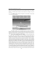
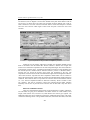
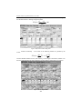
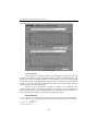
Research Journal of Agricultural Science, 41 (1), 2009
DESIGNING A DRIP IRRIGATION SYSTEM USING HYDROCALC
IRRIGATION PLANNING
PROIECTAREA UNUI SISTEM DE IRIGAŢII PRIN PICURARE UTILIZÂND
PROGRAMUL HYDROCALC
Rareş HĂLBAC-COTOARĂ-ZAMFIR
„Politehnica” University of Timişoara
2nd Victoriei Square, 300006, Timişoara, [email protected]
Abstract: The competitive demand of available
water is more and more acute now in most parts of
the world. The supplies of good water quality are
declining every day. It is, therefore, necessary to
find methods to improve water use efficiency in
agriculture. The drip irrigation is one of the most
efficient irrigation systems that are used in
agriculture. HydroCalc Irrigation Planning is
software for the irrigation community. It is a simple
and easy calculation tool to perform some basic
hydraulic computations. The use of HydroCalc
allows the designer, dealer or end-user to evaluate
the performance of micro irrigation in-field
components, such as: Drip laterals and micro
sprinklers, Sub mains and manifolds, Main lines
(PVC, PE, etc.), Valves Energy calculation.
Rezumat: Cerinţa pentru resursele de apă
disponibilile devine din ce în ce mai acută în
majoritatea ţărilor. Cantităţile existente de apă de
o bună calitate sunt într-o continuă scădere. De
aceea este necesar să fie găsite metode de
îmbunătăţire a eficienţei utilizării apei în sectorul
agricol. Irigaţie prin picurare este una dintre
metodele cele mai eficiente utilizate în agricultură.
Programul de calcul HydroCalc este un software
din comunitatea celor implicaţi în activităţile de
irigare. Reprezintă un instrument simplu pentru
realizarea unor calcule din domeniul hidraulic al
irigaţiilor. Utilizarea acestui program permite
proiectantului, furnizorului de apă dar şi
utilizatorului final să evalueze performanţele
micro-irigaţiei referitor la componentele din câmp
precum picurătoarele laterale şi microaspersoarele, conductele principale (PVC, PE),
etc.
Key words: drip irrigation, HydroCalc, software, water
Cuvinte cheie: irigaţie prin picurare, HydroCalc, program de calcul, apă
INTRODUCTION
Drip irrigation also known as trickle irrigation or micro-irrigation is an irrigation
method that applies water slowly to the roots of plants, by depositing the water either on the
soil surface or directly to the root zone, through a network of valves, pipes, tubing, and
emitters. The goal is to minimize water usage. Drip irrigation may also use devices called
micro-spray heads, which spray water in a small area, instead of emitters. These are generally
used on tree and vine crops. Subsurface drip irrigation or SDI uses permanently or temporarily
buried dripper-line or drip tape. It is becoming more widely used for row crop irrigation
especially in areas where water supplies are limited. The drip irrigation is a slow and frequent
application of water to the soil by means of emitters or drippers located at specific locations /
interval throughout the lateral lines. The emitted water moves through soil mainly by
unsaturated flow. This allows favourable conditions for soil moisture in the root zone and
optimal development of plant. . With this system, the plant can efficiently use available natural
resources such as: soil, water and air. The drip irrigation is also known as “daily irrigation”,
“trickle irrigation”, “daily flow irrigation” or “micro irrigation”. The term “trickle” was
originated in England, “drip” in Israel, “daily flow” in Australia and “micro irrigation” in
420
Research Journal of Agricultural Science, 41 (1), 2009
USA. The difference is only in the name, and all these terms have the same meaning. The
water in a drip irrigation system flows in three forms: It flows continuously throughout the
lateral line; It flows from an emitter or dripper connected to the lateral line; It flows through
orifices perforated in the lateral line.
A well designed drip irrigation system can increase the crop yield due to following
factors: Efficient use of the water (It reduces the direct losses by evaporation, It does not cause
wetting of the leaves, It does not cause movement of drops of water due to the effect of wind, It
reduces consumption of water by grass and weeds, It eliminates surface drainage, It allows
watering the entire field until the edges, It allows applying the irrigation to an exact root depth
of crops, It allows watering greater land area with a specific amount of water), Reaction of the
plant (It increases the yield per unit (hectare-centimetre) of applied water, It improves the
quality of crop and fruit, It allows more uniform crop yield), Environment of the root (It
improves ventilation or aeration, It increases quantity of available nutrients, The conditions are
favourable for retention of water at low tension), Control of pests and diseases (It increases
efficiency of sprayings of insecticides and pesticides, It reduces development of insects and
diseases), Correction of problem of soil salinity (The increase in salts happens at a distance
away from the plant, It reduces salinity problems. A greater reduction is obtained by
increasing the water flow. Salts are limited to an outer periphery of a wetted zone), Weed
control (It reduces the growth of weeds in the shaded humid space), Agronomic
practices
(The activities of the irrigation do not interfere with those of the crop, the plant protection and
the harvesting, It reduces inter cultivation, since there is less growth of weeds, Helps to control
the erosion, It reduces soil compaction, It allows applying fertilizers through the irrigation
water- called fertigation, It increases work efficiency in fruit orchards, because the space
between the rows is maintained dry), Economic benefits (The cost is lower compared with
overhead sprinkler and other permanent irrigation systems, The cost of operation and
maintenance is low. The costs are high when the average row spacing is less than 3 meters, It
can be used in uneven terrains, The water application efficiency is high. Energy use per acre is
reduced due to smaller diameter pipes, and only 50 – 60% of water is used).
MATERIAL AND METHODS
HydroCalc irrigation system planning software is designed to help the user to define
the parameters of an irrigation system. The user will be able to run the program with any
suitable parameters, review the output, and change input data in order to match it to the
appropriate irrigation system set up. Some parameters may be selected from a system list;
whereas other are entered by the user according to their own needs so they do not conflict with
the program’s limitations. The software package includes an opening main window, five
calculation programs, one language setting window and a database that can be modified and
updated by the user.
HydroCalc includes several sub-programs as:
- The Emitters program calculates the cumulative pressure loss, the average flow rate,
the water flow velocity etc. in the selected emitter. It can be changed to suit the desired
irrigation system parameters.
- The SubMain program calculates the cumulative pressure loss and the water flow
velocity in the submain distributing water pipe (single or telescopic). It changes to suit the
required irrigation system parameters.
- The Main Pipe program calculates the cumulative pressure loss and the water flow
velocity in the main conducting water pipe (single or telescopic). It changes to suit the required
irrigation system parameters.
421
Research Journal of Agricultural Science, 41 (1), 2009
- The Shape Wizard program helps transfer the required system parameters (Inlet
Lateral Flow Rate, Minimum Head Pressure) from the Emitters program to the SubMain
program.
- The Valves program calculates the valve friction loss according to the given
parameters.
- The Shifts program calculates the irrigation rate and number of shifts needed
according to the given parameters.
Figure 1. HydroCalc Irrigation Planning
The Emitters program is the first application which can be used in the frame of
HydroCalc software. There are 4 basic type of emitters which can be used: Drip Line, On line,
Sprinklers and Micro-Sprinklers. According to the previous selection the user can opt for a
specific emitter which can be a pressure compensated or a non pressure compensated. Each
emitter has its own set of nominal flow rate values available.
After the previous mentioned fields were completed, the program automatically fills
the following fields: “Inside Diameter”, “KD” and “Exponent”, values which cannot be
changes unless the change will be made in the database. The segment length is next field in
which the user must introduce a value. The end pressure represents the actual value for
calculation of pressure at the furthest emitter. There are some common values for this field:
around 10 m for drippers, around 20 m for mini-sprinklers, between 20 – 30 m for sprinklers
and around 2 m when using the flushing system. There are 2 more options which can be filled
before starting the computation, options which can also be used with their default values. The
Flushing field can be used if the user intends to calculate a system that includes and lateral
flushing. Flushing option will work only in subsequently will be used the “Emitter Line
Length” calculation method. The second option is about topography. Default value is 0%.
Topography field has 2 sub-fields: fixed slope and changing slope. Usually the slopes values
are not exceeding 10%. In many cases the slope is not uniform. The option “Changing” offers
to the user the possibility to determine the altitude along the line, from end line to submain, up
to 10 points each consisting of 2 cells: one for distance one for height. The line of distances is
used to load the distance from the end of the line to the point of the altitude change. These
distances may be unequal. The value of each cell is the net distance from the end of the line
422
Research Journal of Agricultural Science, 41 (1), 2009
point. The value in length in each cell is always greater than the value entered in previous cell.
The lower line, line of “heights” is used to enter altitudes of the point whose distance from the
end of line is set above them. The values may represent elevation readings from a map or
relative elevation to zero level at the end of the line. Positive values mean the point is elevated
above the end of the line while negative values mean the point is below the end of line
elevation.
Figure 2. HydroCalc working sheet before computation procedure
HydroCalc uses for Emitters subprogram a number of 4 calculation methods each of
them in concordance with the loaded data. The first method is “Emitter Line Length” with
which can be realized the computation for the entire designated length. The second method is
represented by “Pressure range”, a calculation which will be executed in a way that makes sure
the maximal pressure variation between maximum emitter’s pressure to minimum emitter’s
pressure does not exceed the pressure range which was introduced by the user. The
computation result will also show the maximum lateral length under the designated conditions.
“Flow Rate Variation” represents the third computation method which can be executed to
achieve the requested flow variation and will generate the maximum lateral length under these
conditions. Flow variation units are in percents. The common values for this field are between
10 – 15%. The last computation method is “Emission Uniformity” which is similar to “flow
rate variation”, and will be executed to achieve the maximum lateral length. Emission
uniformity units are also in percents but the common value for this field is any value above
85%.
RESULTS AND DISCUSSIONS
After were entered all the required values can be launched the “Compute” application.
The cells which are going to be calculated in the emitter window are: Total Emitters, Total
Length, Total Pressure Loss, Pressure Loss, Head Pressure and Velocity per segment. The
additional results report can be reached by pressing the “Additional results” button. This report
contains the following results: Average Emitter Flow Rate, Inlet Lateral Flow Rate, Flow Rate
423
Research Journal of Agricultural Science, 41 (1), 2009
Variation – which is the difference in percentage between the maximum emitter’s discharges to
the minimum emitter’s discharge using the formula:
FV (%) 
Qmax  Qmin
 100
Qmax
Figure 3. HydroCalc results working sheet
Emission uniformity – is the result of the following formula as specified by the
ASAE:
EU (%) 
Qmin
Qmax

CV 
 1  1.27

n

and also Min/Max Emitter Pressure, Inlet Velocity, Total Length, Total Emitters, Emitter Line
Pressures with Head Pressure and End Pressure, Emitter Distance and Emitter Line Pressure.
Figure 4. Results Report Sheet
424
Research Journal of Agricultural Science, 41 (1), 2009
By pressing the “Chart” button it will be displayed the emitter line pressure results
chart. The chart shows the changes of the pressure and flow rate variation along the line.
Figure 5. Chart sheet
CONCLUSIONS
Drip Irrigation is an efficient method of water application in agriculture. The drip
irrigation system allows a constant application of water by drippers at specific locations on the
lateral lines it allows favourable conditions for soil moisture in the root zone and optimal
development of plant. A well designed drip irrigation system can increase the crop yield due to:
efficient use of water, improved microclimate around the root zone, pest control, and weed
control, agronomic and economic benefits.
HydroCalc, by its characteristics, represents a reliable tool in designing a drip
irrigation system. Due to its multiple advantages, this program must be introduced in
universities and research centres for facilitating the work of Romanian researches and also for a
better understanding by students of the problems regarding drip irrigation.
BIBLIOGRAPHY
1. GILARY, ELIEZER, 2008 - HydroCalc Irrigation Planning User Manual, NETAFIM Corporation, Israel;
2. GOYAL, MEGH R., 2007 - Management of drip/ micro or trickle irrigation, University of Puerto Rico,
Puerto Rico
3. H YDROCALC SOFTWARE
4. WWW.NETAFIM.COM
425