Download Agilent 83480A User`s Manual

User's Guide
Agilent 83480A Analyzer,
Agilent 54750A Oscilloscope
Agilent Part No. 83480-90050
Printed in USA June 2000
Agilent Technologies
Lightwave Division
1400 Fountaingrove Parkway
Santa Rosa, CA
95403-1799, USA
(707) 577-1400
HP and Hewlett-Packard are U.S. registered trademarks of Hewlett-Packard
Company.
Notice. The information contained in this document is subject to change
without notice. Agilent Technologies makes no warranty of any kind
with regard to this material, including but not limited to, the implied
warranties of merchantability and tness for a particular purpose. Agilent
Technologies shall not be liable for errors contained herein or for incidental or
consequential damages in connection with the furnishing, performance, or use
of this material.
Restricted Rights Legend. Use, duplication, or disclosure by the U.S.
Government is subject to restrictions as set forth in subparagraph (c) (1) (ii)
of the Rights in Technical Data and Computer Software clause at DFARS
252.227-7013 for DOD agencies, and subparagraphs (c) (1) and (c) (2) of the
Commercial Computer Software Restricted Rights clause at FAR 52.227-19 for
other agencies.
Regulatory Information. The front matter of this book contains regulatory
information.
c Copyright Agilent Technologies 2000
All Rights Reserved. Reproduction, adaptation, or translation without prior
written permission is prohibited, except as allowed under the copyright laws.
Safety Symbols
CAUTION
WARNING
The following safety symbols are used throughout this manual. Familiarize
yourself with each of the symbols and its meaning before operating this
instrument.
The caution sign denotes a hazard to the instrument. It calls attention to a
procedure which, if not correctly performed or adhered to, could result in
damage to or destruction of the instrument. Do not proceed beyond a caution
sign until the indicated conditions are fully understood and met.
The warning sign denotes a life-threatening hazard. It calls attention to a
procedure which, if not correctly performed or adhered to, could result
in injury or loss of life. Do not proceed beyond a warning sign until the
indicated conditions are fully understood and met.
L
Instruction
Manual
The instruction manual symbol. The product is marked with this symbol when it is necessary
for the user to refer to the instructions in the manual.
CE
The CE mark is a registered trademark of the European Community (if accompanied by a year,
it's when the design was proven).
ISM 1-A
This is a symbol of an Industrial Scientic and Medical Group 1 Class A product.
The CSA mark is a registered trademark of the Canadian Standards Association.
j
The line power on symbol.
The line power o symbol.
iii
General Safety Considerations
WARNING
Before this instrument is switched on, make sure it has been properly
grounded through the protective conductor of the ac power cable to a
socket outlet provided with protective earth contact.
Any interruption of the protective (grounding) conductor, inside or
outside the instrument, or disconnection of the protective earth terminal
can result in personal injury.
WARNING
There are many points in the instrument which can, if contacted, cause
personal injury. Be extremely careful.
Any adjustments or service procedures that require operation of the
instrument with protective covers removed should be performed only by
trained service personnel.
WARNING
If this instrument is not used as specied, the protection provided by the
equipment could be impaired. This instrument must be used in a normal
condition (in which all means for protection are intact) only.
WARNING
For continued protection against re hazard, replace line fuse only with
same type and ratings (type nA/nV). The use of other fuses or materials is
prohibited.
WARNING
The power cord is connected to internal capacitors that may remain live
for 5 seconds after disconnecting the plug from its power supply.
CAUTION
Before this instrument is switched on, make sure its primary power circuitry
has been adapted to the voltage of the ac power source.
Failure to set the ac power input to the correct voltage could cause damage to
the instrument when the ac power cable is plugged in.
CAUTION
This is a Safety Class 1 Product (provided with a protective earthing ground
incorporated in the power cord). The mains plug shall only be inserted in a
socket outlet provided with a protective earth contact. Any interruption of
the protective conductor inside or outside of the instrument is likely to make
the instrument dangerous. Intentional interruption is prohibited.
iv
CAUTION
Always use the three-prong ac power cord supplied with this instrument.
Failure to ensure adequate earth grounding by not using this cord may cause
instrument damage.
CAUTION
This instrument is designed for use in INSTALLATION CATEGORY II and
POLLUTION DEGREE 2 per IEC 1010 and 664 respectively.
CAUTION
Ventilation requirements: When installing the instrument in a cabinet,
the convection into and out of the instrument must not be restricted. The
ambient temperature (outside the cabinet) must be less than the maximum
operating temperature of the instrument by 4 C for every 100 watts
dissipated in the cabinet. If the total power dissipated in the cabinet is
greater than 800 watts, then forced convection must be used.
CAUTION
The input circuits can be damaged by electrostatic discharge (ESD). Repair
of damage due to misuse is not covered under warranty. Therefore, avoid
applying static discharges to the front-panel input connectors. Before
connecting any coaxial cable to the connectors, momentarily short the center
and outer conductors of the cable together. Avoid touching the front-panel
input connectors without rst touching the frame of the instrument. Be sure
the instrument is properly earth-grounded to prevent buildup of static charge.
The electrical ports of plug-in modules, used with the Agilent 83480A and
Agilent 54750A, are very sensitive to electrostatic discharge.
NOTE
This instrument has been designed and tested in accordance with IEC Publication 1010.1, and has been
supplied in a safe condition. The instruction documentation contains information and warnings which
must be followed by the user to ensure safe operation and to maintain the instrument in a safe
condition.
v
NOTE
Clean the cabinet using a damp cloth only.
vi
Certication
Agilent Technologies certies that this product met its published specications
at the time of shipment from the factory. Agilent Technologies further
certies that its calibration measurements are traceable to the United States
National Institute of Standards and Technology, to the extent allowed by
the Institute's calibration facility, and to the calibration facilities of other
International Standards Organization members.
vii
X-Ray Radiation Notice
viii
Declaration of Conformity
ix
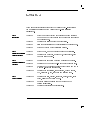
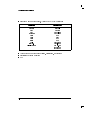
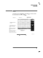
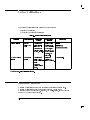
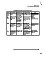
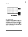
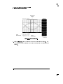
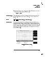
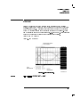
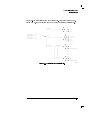
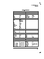
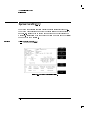
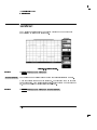
Additional Information The following table lists additional performance information for the EMC
product specications listed in the Declaration of Conformity.
EMC Product Specication
Performance Code
PASS - Temporary degradation, self-recoverable.
IEC 801-2:1991 /EN 50082-1 (1992): 4kV CD, 8kV AD
PASS - Temporary degradation, self-recoverable.
IEC 801-3:1984 /EN 50082-1 (1992); 3 V/m, (1 kHz 80%
AM, 27-1000 MHz)
IEC 801-4:1988 /EN 50082-1 (1992): 0.5 kV Sig Lines, 1kV PASS - Normal operation, no eect.
Power Lines
x
Warranty
This Agilent Technologies instrument product is warranted against defects in
material and workmanship for a period of one year from date of shipment.
During the warranty period, Agilent Technologies will, at its option, either
repair or replace products which prove to be defective.
For warranty service or repair, this product must be returned to a service
facility designated by Agilent Technologies. Buyer shall prepay shipping
charges to Agilent Technologies and Agilent Technologies shall pay shipping
charges to return the product to Buyer. However, Buyer shall pay all shipping
charges, duties, and taxes for products returned to Agilent Technologies from
another country.
Agilent Technologies warrants that its software and rmware designated by
Agilent Technologies for use with an instrument will execute its programming
instructions when properly installed on that instrument. Agilent Technologies
does not warrant that the operation of the instrument, or software, or
rmware will be uninterrupted or error-free.
Limitation of Warranty
The foregoing warranty shall not apply to defects resulting from improper
or inadequate maintenance by Buyer, Buyer-supplied software or
interfacing, unauthorized modication or misuse, operation outside of the
environmental specications for the product, or improper site preparation
or maintenance.
NO OTHER WARRANTY IS EXPRESSED OR IMPLIED. AGILENT
TECHNOLOGIES SPECIFICALLY DISCLAIMS THE IMPLIED WARRANTIES
OF MERCHANTABILITY AND FITNESS FOR A PARTICULAR PURPOSE.
Exclusive Remedies
THE REMEDIES PROVIDED HEREIN ARE BUYER'S SOLE AND EXCLUSIVE
REMEDIES. AGILENT TECHNOLOGIES SHALL NOT BE LIABLE FOR
ANY DIRECT, INDIRECT, SPECIAL, INCIDENTAL, OR CONSEQUENTIAL
DAMAGES, WHETHER BASED ON CONTRACT, TORT, OR ANY OTHER
LEGAL THEORY.
xi
Assistance
CAUTION
Product maintenance agreements and other customer assistance agreements
are available for Agilent Technologies products.
For any assistance, contact your nearest Agilent Technologies Sales and
Service Oce.
When an instrument is returned to a Agilent Technologies service oce for
servicing, it must be adequately packaged and have a complete description of
the failure symptoms attached.
When describing the failure, please be as specic as possible about the nature
of the problem. Include copies of additional failure information (such as
instrument failure settings, data related to instrument failure, and error
messages) along with the instrument being returned.
Please notify the service oce before returning your instrument for service.
Any special arrangements for the instrument can be discussed at this time.
This will help the Agilent Technologies service oce repair and return your
instrument as quickly as possible.
The original shipping containers should be used. If the original materials
were not retained, identical packaging materials are available through any
Agilent Technologies oce.
Instrument damage can result from using packaging materials other than the
original materials. Never use styrene pellets as packaging material. They
do not adequately cushion the instrument or prevent it from shifting in
the carton. They may also cause instrument damage by generating static
electricity.
Sales and service oces
Agilent Technologies has sales and service oces located around the world
to provide complete support for Agilent Technologies products. To obtain
servicing information or to order replacement parts, contact the nearest
xii
Agilent Technologies Sales and Service Oce. In any correspondence or
telephone conversation, refer to the instrument by its model number, serial
number, and option designation.
Before returning an instrument for service, call the Agilent
Technologies Instrument Support Center at (800) 403-0801,
visit the Test and Measurement Web Sites by Country page at
http://www.tm.agilent.com/tmo/country/English/index.html, or call one of the
numbers listed below.
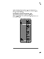
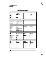
Agilent Technologies Service Numbers
Austria
Belgium
Brazil
China
Denmark
Finland
France
Germany
India
Italy
Ireland
Japan
Korea
Mexico
Netherlands
Norway
Russia
Spain
Sweden
Switzerland
United Kingdom
United States and Canada
01/25125-7171
32-2-778.37.71
(11) 7297-8600
86 10 6261 3819
45 99 12 88
358-10-855-2360
01.69.82.66.66
0180/524-6330
080-34 35788
+39 02 9212 2701
01 615 8222
(81)-426-56-7832
82/2-3770-0419
(5) 258-4826
020-547 6463
22 73 57 59
+7-095-797-3930
(34/91) 631 1213
08-5064 8700
(01) 735 7200
01 344 366666
(800) 403-0801
xiii
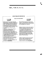
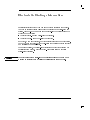
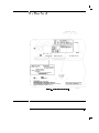
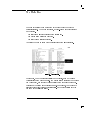
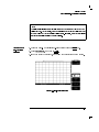
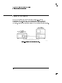
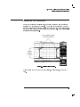
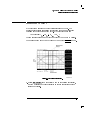
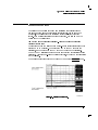
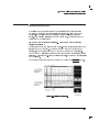
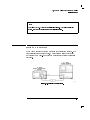
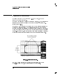
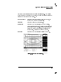
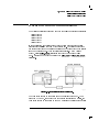
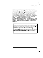
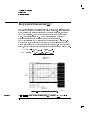
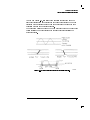
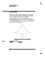
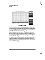
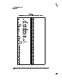
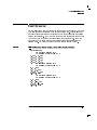
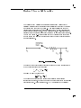
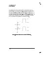
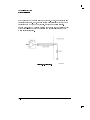
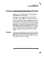
Electrostatic Discharge Information
Electrostatic discharge (ESD) can damage or destroy electronic components.
All work on electronic assemblies should be performed at a static-safe work
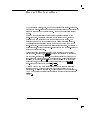
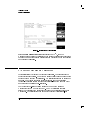
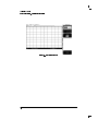
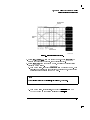
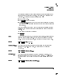
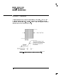
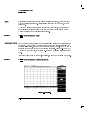
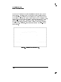
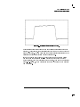
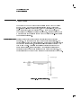
station. Figure 0-1 shows an example of a static-safe work station using two
types of ESD protection:
Conductive table-mat and wrist-strap combination.
Conductive oor-mat and heel-strap combination.
Both types, when used together, provide a signicant level of ESD protection.
Of the two, only the table-mat and wrist-strap combination provides adequate
ESD protection when used alone.
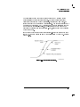
To ensure user safety, the static-safe accessories must provide at least 1 M
of isolation from ground. Refer to Table 0-1 for information on ordering
static-safe accessories.
WARNING
These techniques for a static-safe work station should not be used when
working on circuitry with a voltage potential greater than 500 volts.
xiv
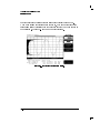
Figure 0-1. Example of a static-safe work station.
xv
Reducing ESD Damage The following suggestions may help reduce ESD damage that occurs during
testing and servicing operations.
Personnel should be grounded with a resistor-isolated wrist strap before
removing any assembly from the unit.
Be sure all instruments are properly earth-grounded to prevent a buildup of
static charge.
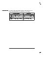
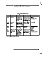
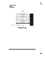
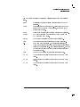
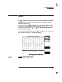
Table 0-1 lists static-safe accessories that can be obtained from Agilent
Technologies using the Agilent part numbers shown.
Table 0-1. Static-Safe Accessories
Agilent Part
Number
Description
9300-0797
Set includes: 3M static control mat 0.6 m 2 1.2 m (2 ft 2 4 ft) and 4.6 cm (15 ft) ground
wire. (The wrist-strap and wrist-strap cord are not included. They must be ordered separately.)
Wrist-strap cord 1.5 m (5 ft)
Wrist-strap, color black, stainless steel, without cord, has four adjustable links and a 7 mm
post-type connection.
ESD heel-strap (reusable 6 to 12 months).
9300-0980
9300-1383
9300-1169
xvi
Lightwave Connector Care
CAUTION
Improper connector care, cleaning, or use of mismatched cable connectors
can invalidate the published specications and damage connectors. Clean all
cables before applying to any connector. Repair of damaged connectors due to
improper use is not covered under warranty.
Introduction
Lightwave cable interfaces can be damaged by improper cleaning and
connection procedures. Dirty or damaged lightwave interfaces can result in
nonrepeatable or inaccurate measurements. This chapter will suggest some
best practices to clean, care for, connect, and inspect lightwave connectors.
Lightwave connectors are used to connect two ber ends together. These
connections may be used to join cables between optical ports on devices, laser
sources, receivers, patch panels, terminals and many other types of systems
or components.
Fiber optic cables are used at dierent wavelengths, in single or multimode,
and in dierent environments. There are a variety of sizes, core/cladding
combinations, jackets, and indexes of refraction. In general, dierent types
of cables do not work well together. Cables should match each other and the
system.
However, regardless of the cable type, the connectors have only one function:
to provide a direct and low-loss optical signal transition from one ber end
to another. When these connectors are used in a measurement system,
repeatability becomes an important factor.
Lightwave connectors dier from electrical or microwave system
connectors. In a ber optic system, light is transmitted through an extremely
small ber core. Because ber cores are often 62.5 microns (0.0625 mm) or
less in diameter, and dust particles range from tenths of a micron to several
microns in diameter, dust and very minute contamination on the end of the
ber core can degrade the performance of the connector interface (where the
two cores meet). Therefore, the connector must be precisely aligned and the
connector interface free of trapped foreign material.
Connector (or insertion) loss is one important performance characteristic
of a lightwave connector. Typical values are less than 1 dB of loss, and
sometimes as little as 0.1 dB of loss with high performance connectors.
xvii
Return loss is another important factor. It is a measure of reection. The less
reection the better, (the larger the return loss, the smaller the reection).
The best physically contacting connectors have return losses better than
50 dB, although 30 to 40 dB is more common.
Causes of connector loss and reections include core misalignment,
dierences in the numerical aperture of two bers, spacing and air gaps,
reections caused by damaged, worn, or loose ber ends, and the improper
use and removal of index matching compounds.
Achieving the best possible connection, where the ber end faces are ush
(no air gap) and properly aligned, depends on two things:
1. the type of connector
2. using the proper cleaning and connecting techniques. If the connection is
lossy or reective, light will not make a smooth transition. If the transition
is not smooth or the connection is not repeatable, measurement data will
be less accurate. For this reason, lightwave connections can make a critical
dierence in optical measurement systems.
xviii
Cleaning and handling Proper cleaning and handling of lightwave connectors is imperative for
achieving accurate and repeatable measurements with your Agilent
Technologies lightwave equipment. Lightwave interfaces should be cleaned
before each measurement using the techniques described in this handbook.
Information on protecting and storing your connectors/cables and tips on how
to properly mate connectors are also included in this section.
Denition of terms
To avoid confusion, the following denitions are used in this handbook.
Connector
Houses the ber end, most open at the end of a lightwave
cable or on the front panel of an instrument or accessory.
Adapter
Does not contain optical ber. Used to mate two optical
connectors.
Handling
Always handle lightwave connectors and cable ends with great care. Fiber
ends should never be allowed to touch anything except other mating surfaces
or cleaning solutions and tools.
Always keep connectors and cable ends covered with a protective cap when
they are not in use. (See \Storage.")
Cleaning
CAUTION
Two cleaning processes are provided. The rst process describes how to clean
non-lensed lightwave connectors. The second process describes how to clean
lightwave adapters.
Agilent Technologies strongly recommends index matching compounds NOT
be applied to their instruments and accessories. Some compounds, such as
gels, may be dicult to remove and can contain damaging particulates. If
you think the use of such compounds is necessary, refer to the compound
manufacturer for information on application and cleaning procedures.
xix
Cleaning non-lensed
lightwave connectors
CAUTION
Equipment
The following is a list of the items that should be used to clean non-lensed
lightwave connectors.
Pure isopropyl alcohol : : : : : : : : : : : : : : : : : : : : : : : : : : : : : : : : : : : : : : : : : : : : : : : : : : : : {
Cotton swabs : : : : : : : : : : : : : : : : : : : : : : : : : : : : : : Agilent part number 8520-0023
Foam swabs : : : : : : : : : : : : : : : : : : : : : : : : : : : : : : : : Agilent part number 9300-1223
Compressed air : : : : : : : : : : : : : : : : : : : : : : : : : : : : Agilent part number 8500-5262
Agilent Technologies recommends you do not use any type of foam swab
to clean optical ber cable ends. Foam swabs can leave lmy deposits on
ber ends that can degrade performance. However, foam is required to clean
inside bulk head connectors.
Process
CAUTION
Before cleaning the ber end, clean the ferrules and other parts of the
connector. Use isopropyl alcohol, clean cotton swabs, and clean compressed
air. Then use alcohol to clean the ber end. Some amount of wiping or mild
scrubbing of the ber end can help remove particles when application of
alcohol alone will not remove them. This can be done by applying the alcohol
to a cotton swab and moving it back and forth across the ber end several
times. This technique can help remove or displace particles smaller than one
micron.
Allow the connector to dry (about a minute) or dry it immediately with clean
compressed air. Compressed air lessens the chance of deposits remaining on
the ber end after the alcohol evaporates. It should be blown horizontally
across the ber end. Visually inspect the ber end for stray cotton bers. As
soon as the connector is dry, the connection should be made.
Inverting the compressed air canister while spraying will produce residue on
the sprayed surface. Refer to instructions provided on the compressed air
canister.
xx
Cleaning lightwave
adapters
Equipment
All of the items listed above for cleaning connectors may be used to clean
lightwave adapters. In addition, small foam swabs may be used along
with isopropyl alcohol and compressed air to clean the inside of lightwave
connector adapters.
NOTE
As noted in a previous caution statement, the foam swabs can leave lmy deposits. These deposits
are very thin however, and the risk of other contamination buildup on the inside of adapters greatly
outweighs the risk of contamination of foam swab deposits left from cleaning the inside of adapters.
Process
Clean the adapter by applying isopropyl alcohol to the inside of the connector
with a foam swab. Allow the adapter to air dry, or dry it immediately with
clean compressed air.
Storage
All of Agilent Technologies' lightwave instruments are shipped with either
laser shutter caps or dust caps on the lightwave adapters that come with the
instrument. Also, all of the cables that are shipped have covers to protect the
cable ends from damage or contamination. These dust caps and protective
covers should be kept on the equipment except when in use.
Making connections
Proper connection technique requires attention to connector compatibility,
insertion technique and torque requirements. Connectors must be the same
connector type in order to ensure mechanical and optical compatibility.
Attempting to connect incompatible connector types may prevent the
connection from functioning properly and even cause damage to the ber
surfaces. A visual inspection of the mechanical interfaces may not be
enough because some connector types have the same mechanical interface
but have dierent optical ber interfaces (for example, angled-no-contact,
angled-contact or straight-contact ber interfaces). Refer to the
manufacturer's data sheet to conrm connector type compatibility before
connecting.
xxi
CAUTION
Summary
When you insert the ferrule into an adapter, make sure the ber end does
not touch the outside of the mating adapter. This ensures you will not rub
the ber end against any undesirable surface. Many connectors have a keyed
slot provided for optimum measurement repeatability that also helps to align
and seat the two connectors. After the ferrule is properly seated inside the
other connector, use one hand to keep it straight, rotate it to align the key,
and tighten it with the other hand.
Most connectors using springs to push ber ends together exert one to two
pounds of force. Over-tightening or under-tightening these connectors can
result in misalignment and nonrepeatable measurements. Always nger
tighten the connector in a consistent manner. Refer to the manufacturer's
data sheet for any torque recommendations.
OPTION 3XX INSTRUMENTS: To avoid damage, handle the pigtail ber with
care. Use only an appropriate ber cleaver tool for cutting the ber. Do
not pull the bare ber out of its jacket, crush it, kink it, or bend it past its
minimum bend radius.
When making measurements with lightwave instruments or accessories,
the following precautions will help to insure good, reliable, repeatable
measurements:
Conrm connector type compatibility.
Use extreme care in handling all lightwave cables and connectors.
Be sure the connector interfaces are clean before making any connections.
Use the cleaning methods described in this handbook.
Keep connectors and cable ends covered when not in use.
xxii
Inspection
Visual inspection
Although it is not necessary, visual inspection of ber ends can be helpful.
Contamination and/or imperfections on the cable endface can be detected as
well as cracks or chips in the ber itself.
Several ber inspection scopes are on the market, but any microscope with
an enlargement range of 100X to 200X can be used. It is helpful to devise
some method to hold the ber in place while viewing in this range.
Inspect the entire endface for contamination, raised metal, or dents in the
metal, as well as any other imperfections. Inspect the ber core for cracks
and chips.
Visible imperfections not touching the ber core may not aect the
performance of the lightwave connection (unless the imperfections keep
the bers from contacting). Consistent optical measurements are the best
assurance that your lightwave connection is performing properly.
WARNING
Always remove both ends of ber-optic cables from any instrument,
system, or device before visually inspecting the ber ends. Disable all
optical sources before disconnecting ber-optic cables. Failure to do so
may result in permanent injury to your eyes.
Optical performance
testing
Introduction
Consistent measurements with your lightwave equipment are a good
indication that you have good connections. However, you may wish to know
the insertion loss and/or return loss of your lightwave cables or accessories. If
you test your cables and accessories for insertion loss and return loss upon
receipt, and retain the measured data for comparison, you will be able to tell
in the future if any degradation has occurred.
Insertion loss
Insertion loss can be tested using a number of dierent test equipment
congurations. Some of these are:
an Agilent 8702B or Agilent 8703A lightwave component analyzer system
with a lightwave source and receivers
an Agilent 83420 lightwave test set with an Agilent 8510 network analyzer
xxiii
an Agilent 8153A lightwave multimeter with a source and a power sensor
module
Many other possibilities exist. The basic requirements are an appropriate
lightwave source and a compatible lightwave receiver. Refer to the manuals
provided with your lightwave test equipment for information on how to
perform an insertion loss test.
Typical insertion loss for cables is less than 1 dB, and can be as little as
0.1 dB. For actual specications on your particular cable or accessory, refer to
the manufacturer.
Return loss
Return loss can be tested using a number of dierent test equipment
congurations. Some of these are:
an Agilent 8703A lightwave component analyzer
an Agilent 8702B lightwave component analyzer with the appropriate
source, receiver and lightwave coupler
an Agilent 8504B precision reectometer
an Agilent 8153A lightwave multimeter and Agilent 81534A return loss
module
Many other possibilities exist. The basic requirements are an appropriate
lightwave source, a compatible lightwave receiver, and a compatible
lightwave coupler.
Refer to the manuals provided with your lightwave test equipment for
information on how to perform a return loss test.
Typical return loss for single mode units is better than 40 dB. For actual
specications on your particular cable or accessory, refer to the manufacturer.
xxiv
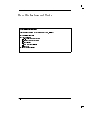
In This Book
This manual provides information about the Agilent 83480A-series digital
communications analyzers and the Agilent 54750A-series digitizing
oscilloscopes.
Part 1
Introduction
Chapter 1
Chapter 2
Chapter 3
Chapter 4
gives you a brief overview of the instrument and describes
the menu and key conventions and the front and rear panels
of the instrument.
describes the front panel keys and functions.
lists the specications and characteristics of the instrument.
gives an overview of the calibration options.
Part 2
Chapter 5
Digital Communications Chapter 6
Analyzer Functions
gives the eye, mask and eyeline measurement tutorials.
describes the mask test, measure eye, channel setup, time
base and trigger menus.
Chapter 7
Part 3
Digitizing Oscilloscope Chapter 8
Functions
describes the automatic waveform measurement process.
describes how to use the built-in automatic measurements.
describes how to increase measurement accuracy and how to
make time-interval measurements.
describes the acquisition, channel setup, dene measure,
FFT, histogram, math, time base and trigger menus.
Chapter 9
Chapter 10
Part 4
System Functions
Chapter 11
Chapter 12
Chapter 13
describes the disk, display, limit test, marker, setup, setup
print, utility and waveform menus.
provides a list of messages that may appear on the
instrument's display.
describes basic instrument architecture.
xxv
Contents
Sales and service oces
. . . . . . . . . . . . . .
1. The Instrument at a Glance
xii
.
.
.
.
.
.
.
.
.
.
.
.
.
.
.
.
.
.
.
.
.
.
.
.
.
.
.
.
.
.
.
.
.
.
.
.
.
.
.
.
.
.
.
.
.
.
.
.
.
.
.
.
.
.
.
.
.
.
.
.
.
.
.
.
.
.
.
.
.
.
.
.
.
.
.
.
.
.
.
.
.
.
.
.
.
.
.
.
.
.
.
.
.
.
.
.
.
.
.
.
.
.
.
.
.
.
.
.
.
.
.
.
1-5
1-7
1-9
1-10
1-11
1-13
1-14
1-15
.
.
.
.
.
.
.
.
.
.
.
.
.
.
.
.
.
.
.
.
.
.
.
.
.
.
.
.
.
.
.
.
.
.
.
.
.
.
.
.
.
.
.
.
.
.
.
.
.
.
.
.
.
.
.
.
.
.
.
.
.
.
.
.
.
.
.
.
.
.
.
.
.
.
.
.
.
.
.
.
.
.
.
.
2-3
2-4
2-5
2-6
2-7
2-8
Horizontal System . . . . . . . . . . . . . . . .
Trigger Specications Electrical and Optical Channels
Standard instrument, 2.5 GHz mode . . . . . . .
Option 100, 12 GHz mode . . . . . . . . . . .
Option 100, 12 GHz/Gate mode . . . . . . . . .
General Specications . . . . . . . . . . . . . .
.
.
.
.
.
.
.
.
.
.
.
.
3-3
3-4
3-4
3-5
3-5
3-6
.
.
.
.
.
.
.
.
.
.
.
.
.
.
.
.
4-4
4-4
4-6
4-8
4-10
4-12
4-13
4-15
Ordering Information . .
Menu and Key Conventions
The Front Panel . . . . .
4Autoscale5 . . . . . . .
Display . . . . . . .
Entry devices . . . . .
Indicator lights . . . .
The Rear Panel . . . . .
2. General Purpose Keys
The Clear Display Key
The Fine Function .
The Help Key . . . .
The Local Key . . .
The Run Key . . . .
The Stop/Single Key
NNNNNNNNNNNNNN
.
.
.
.
.
.
.
.
.
.
.
.
3. Specications and Characteristics
4. Calibration Overview
Factory Calibrations . . . . . . . . . .
Mainframe Calibration . . . . . . . .
O/E Factory Wavelength Calibration .
User Calibrations|Optical and Electrical
O/E User-Wavelength Calibration . . .
Plug-in Module Vertical Calibration . .
Oset Zero Calibration . . . . . . . .
Dark Calibration . . . . . . . . . .
.
.
.
.
.
.
.
.
.
.
.
.
.
.
.
.
.
.
.
.
.
.
.
.
.
.
.
.
.
.
.
.
.
.
.
.
.
.
.
.
Contents-1
Channel Skew Calibration . . . . . . . . . . . . .
Probe Calibration . . . . . . . . . . . . . . . . . . .
External Scale . . . . . . . . . . . . . . . . . .
Complete Calibration Summary . . . . . . . . . . . .
5. Eye, Mask and Eyeline Mode Measurement Tutorials
Making Eye Diagram Measurements . . . . . . . . . .
Setting up the system . . . . . . . . . . . . . . .
Positioning the waveform . . . . . . . . . . . . . .
Making the measurement . . . . . . . . . . . . . .
Measuring extinction ratio . . . . . . . . . . . . .
Measuring eye height . . . . . . . . . . . . . . .
Measuring crossing % . . . . . . . . . . . . . . .
Measuring eye width . . . . . . . . . . . . . . . .
Measuring jitter . . . . . . . . . . . . . . . . . .
Measuring duty cycle distortion . . . . . . . . . . .
Measuring Q-factor . . . . . . . . . . . . . . . .
Measuring rise time . . . . . . . . . . . . . . . .
Measuring fall time . . . . . . . . . . . . . . . .
Testing to a Mask . . . . . . . . . . . . . . . . . .
Setting up the system . . . . . . . . . . . . . . .
Positioning the waveform . . . . . . . . . . . . . .
Making the measurement . . . . . . . . . . . . . .
Standard Mask . . . . . . . . . . . . . . . . . .
Making Eyeline Measurements (Agilent 83480A Option 001
only) . . . . . . . . . . . . . . . . . . . . . .
Eyeline traces . . . . . . . . . . . . . . . . . . .
Noise reduction . . . . . . . . . . . . . . . . . .
Error trace capture . . . . . . . . . . . . . . . .
Equipment conguration/program installation . . . .
Error trace capture . . . . . . . . . . . . . . . .
6. The Digital Communications Analysis Menus
Mask Test Menu
NNNNNNNNNNNNNNNNNNNNNNNNNNNNNNNN
. .
.
.
.
.
.
Scale Mask . .
Mask Align . .
Align Mode . .
Run... . . . .
Fail action...
NNNNNNNNNNNNNNNNNNNNNNNNNNNNNNNN
NNNNNNNNNNNNNNNNNNNNNNNNNNNNNNNN
NNNNNNNNNNNNNNNNNNNN
NNNNNNNNNNNNNNNNNNNNNNNNNNNNNNNNNNNNNNNNNNNN
Contents-2
.
.
.
.
.
.
.
.
.
.
.
.
.
.
.
.
.
.
.
.
.
.
.
.
.
.
.
.
.
.
.
.
.
.
.
.
.
.
.
.
.
.
.
.
.
.
.
.
.
.
.
.
.
.
.
.
.
.
.
.
.
.
.
.
.
.
.
.
.
.
.
.
.
.
.
.
.
.
.
.
.
.
.
.
.
.
.
.
.
.
.
.
.
.
.
.
4-16
4-17
4-19
4-21
5-3
5-4
5-5
5-9
5-10
5-13
5-14
5-15
5-16
5-17
5-19
5-21
5-23
5-25
5-27
5-28
5-31
5-32
5-37
5-38
5-40
5-42
5-43
5-49
6-3
6-19
6-21
6-22
6-23
6-25
Measure Eye Menu
. . . . . . . . . . . . . . . . .
Extinction ratio... . . . . .
Eye height . . . . . . . . .
Crossing % . . . . . . . . .
Eye width . . . . . . . . . .
Jitter . . . . . . . . . . .
Duty cycle distortion... . .
Q-factor . . . . . . . . . .
NNNNNNNNNNNNNNNNNNNNNNNNNNNNNNNNNNNNNNNNNNNNNNNNNNNNNNNNNNN
NNNNNNNNNNNNNNNNNNNNNNNNNNNNNNNN
NNNNNNNNNNNNNNNNNNNNNNNNNNNNNNNN
NNNNNNNNNNNNNNNNNNNNNNNNNNNNN
NNNNNNNNNNNNNNNNNNNN
NNNNNNNNNNNNNNNNNNNNNNNNNNNNNNNNNNNNNNNNNNNNNNNNNNNNNNNNNNNNNNNNNNNNNNNNNN
NNNNNNNNNNNNNNNNNNNNNNNNNN
Channel Setup Menu
Time Base Menu .
Units . . . . .
Bit Rate . . .
Scale . . . . .
Position . . .
Reference . . .
NNNNNNNNNNNNNNNNN
NNNNNNNNNNNNNNNNNNNNNNNNNN
NNNNNNNNNNNNNNNNN
NNNNNNNNNNNNNNNNNNNNNNNNNN
NNNNNNNNNNNNNNNNNNNNNNNNNNNNN
.
.
.
.
.
.
.
.
.
.
.
.
.
.
.
.
.
.
.
.
.
.
.
.
.
.
.
.
NNNNNNNNNNNNNNNNNNNNNNNNNNNNNNNNNNNNNNNNNNNNNNNNNNNNNNNNNNNNNNNNNNNN
Time base windowing...
Window Position
.
NNNNNNNNNNNNNNNNNNNNNNNNNNNNNNNNNNNNNNNNNNNNNNN
Trigger Menu .
Trigger Basics
Sweep . . .
Source . .
NNNNNNNNNNNNNNNNN
NNNNNNNNNNNNNNNNNNNN
.
.
.
.
.
.
.
.
NNNNNNNNNNNNNNNNNNNNNNNNNNNNNNNNNNNNNNNNNNNN
External Scale
Level . . . . .
Slope . . . . .
Hysteresis . .
Trig Bandwidth
NNNNNNNNNNNNNNNNN
NNNNNNNNNNNNNNNNN
NNNNNNNNNNNNNNNNNNNNNNNNNNNNNNNN
NNNNNNNNNNNNNNNNNNNNNNNNNNNNNNNNNNNNNNNNNNNN
.
.
.
.
.
.
.
.
.
.
.
.
.
.
.
.
.
.
.
.
.
.
.
.
.
.
.
.
.
.
.
.
.
.
.
.
.
.
.
.
.
.
.
.
.
.
.
.
.
.
.
.
.
.
.
.
.
.
.
.
.
.
.
.
.
.
.
.
.
.
.
.
.
.
.
.
.
.
.
.
.
.
.
.
.
.
.
.
.
.
. . . . . . . . . .
.
.
.
.
.
.
.
.
.
.
.
.
.
.
.
.
.
.
.
.
.
.
.
.
.
.
.
.
.
.
.
.
.
.
.
.
.
.
.
.
.
.
.
.
.
.
.
.
.
.
.
.
.
.
.
.
.
.
.
.
.
.
.
.
.
.
.
.
.
.
.
.
.
.
.
.
.
.
.
.
.
.
.
.
.
.
.
.
.
.
.
.
.
.
.
.
.
.
.
.
.
.
.
.
.
.
.
.
.
.
.
.
.
.
.
.
.
.
.
.
.
.
.
.
.
.
.
.
.
.
.
.
.
.
.
.
.
.
.
.
.
.
.
.
.
.
.
.
.
.
.
.
.
.
.
.
.
.
.
.
.
.
.
.
.
.
.
.
.
.
.
.
.
.
.
.
.
.
.
.
.
.
.
.
.
.
.
.
.
.
.
.
.
.
.
.
.
.
.
.
.
.
.
.
.
.
.
.
.
.
.
.
.
.
.
.
.
.
.
.
.
.
.
.
.
.
.
.
.
.
.
.
.
.
.
.
.
.
.
.
6-30
6-32
6-35
6-36
6-38
6-39
6-40
6-41
6-43
6-44
6-45
6-45
6-46
6-46
6-47
6-48
6-49
6-50
6-50
6-51
6-51
6-52
6-52
6-52
6-53
6-53
Contents-3
7. Waveform Measurements
How to Make Waveform Measurements . . . . .
The Waveform Measurement Process . . . . .
Data collection . . . . . . . . . . . . . .
Building a histogram . . . . . . . . . . . .
Calculating min and max from the data record
Calculating top and base . . . . . . . . . .
Locating crossing points . . . . . . . . . .
.
.
.
.
.
.
.
.
.
.
.
.
.
.
.
.
.
.
.
.
.
.
.
.
.
.
.
.
Determining rising and falling edges . . . .
Standard Waveform Denitions . . . . . . .
Voltage and power measurements . . . . .
Timing denitions . . . . . . . . . . . .
User-dened 1time . . . . . . . . . . .
Some important measurement considerations
.
.
.
.
.
.
.
.
.
.
.
.
.
.
.
.
.
.
.
.
.
.
.
.
7-3
7-4
7-5
7-6
7-7
7-8
7-9
7-10
7-11
7-14
7-14
7-17
7-19
7-20
. . . . .
. . . . .
8-3
8-4
Calculating thresholds . . . . . . . . . . . . . . . . .
8. Making Automatic Measurements
Period and frequency measurements . . . .
Pulse width measurements . . . . . . . .
Rise time, fall time, preshoot, and overshoot
measurements . . . . . . . . . . . .
Front Panel Measure Section . . . . . . . .
1time . . . . . . . . . . . . . . . . .
+width . . . . . . . . . . . . . . . .
0width . . . . . . . . . . . . . . . .
Duty Cycle . . . . . . . . . . . . . .
Fall Time . . . . . . . . . . . . . . .
Frequency . . . . . . . . . . . . . . .
Overshoot . . . . . . . . . . . . . . .
Period . . . . . . . . . . . . . . . .
Preshoot . . . . . . . . . . . . . . .
Rise Time . . . . . . . . . . . . . . .
Vamp . . . . . . . . . . . . . . . . .
Vbase . . . . . . . . . . . . . . . . .
Vpp . . . . . . . . . . . . . . . . . .
Vrms . . . . . . . . . . . . . . . . .
NNNNNNNNNNNNNNNNN
NNNNNNNNNNNNNNNNNNNN
NNNNNNNNNNNNNNNNNNNNN
NNNNNNNNNNNNNNNNNNNNNNNNNNNNNNNN
NNNNNNNNNNNNNNNNNNNNNNNNNNNNN
NNNNNNNNNNNNNNNNNNNNNNNNNNNNN
NNNNNNNNNNNNNNNNNNNNNNNNNNNNN
NNNNNNNNNNNNNNNNNNNN
NNNNNNNNNNNNNNNNNNNNNNNNNN
NNNNNNNNNNNNNNNNNNNNNNNNNNNNN
NNNNNNNNNNNNNN
NNNNNNNNNNNNNNNNN
NNNNNNNNNNN
NNNNNNNNNNNNNN
Contents-4
.
.
.
.
.
.
.
.
.
.
.
.
.
.
.
.
.
.
.
.
.
.
.
.
.
.
.
.
.
.
.
.
.
.
.
.
.
.
.
.
.
.
.
.
.
.
.
.
.
.
.
.
.
.
.
.
.
.
.
.
.
.
.
.
.
.
.
.
.
.
.
.
.
.
.
.
.
.
.
.
.
.
.
.
.
.
8-4
8-5
8-5
8-6
8-6
8-6
8-7
8-7
8-7
8-8
8-8
8-8
8-9
8-9
8-9
8-10
NNNNNNNNNNNNNN
Vtop
. . . . . . . . . . . . . . . . . . . . . .
General Meas Menu . . . . . . . . . . . . . . . . . . .
NNNNNNNNNNNNNN
Tmax .
Tmin .
Vavg .
Vlower
Vmiddle
Vupper
. . . .
. . . .
. . . .
. . . .
. . . .
. . . .
Avg Power Menu .
Avg Power . . .
Freq Domain Menu
FFT freq . . .
FFT mag . . . .
FFT 1freq . . .
FFT 1mag . . .
Source . . . .
Peak number . .
Pk threshold .
Histogram Menu .
61 . . . . .
62 . . . . .
63 . . . . .
hits . . . . .
mean . . . . .
median . . . .
peak . . . . .
pk-pk . . . . .
std dev . . . .
NNNNNNNNNNNNNN
NNNNNNNNNNNNNN
NNNNNNNNNNNNNNNNNNNN
NNNNNNNNNNNNNNNNNNNNNNN
NNNNNNNNNNNNNNNNNNNN
NNNNNNNNNNNNNNNNNNNNNNNNNNNNN
NNNNNNNNNNNNNNNNNNNNNNNNNN
NNNNNNNNNNNNNNNNNNNNNNN
NNNNNNNNNNNNNNNNNNNNNNNNNNNNN
NNNNNNNNNNNNNNNNNNNNNNNNNN
NNNNNNNNNNNNNNNNNNNN
NNNNNNNNNNNNNNNNNNNNNNNNNNNNNNNNNNN
NNNNNNNNNNNNNNNNNNNNNNNNNNNNNNNNNNNNNN
NNNNNNNNNNNNNNN
NNNNNNNNNNNNNNN
NNNNNNNNNNNNNNN
NNNNNNNNNNNNNN
NNNNNNNNNNNNNN
NNNNNNNNNNNNNNNNNNNN
NNNNNNNNNNNNNN
NNNNNNNNNNNNNNNNN
NNNNNNNNNNNNNNNNNNNNNNN
.
.
.
.
.
.
.
.
.
.
.
.
.
.
.
.
.
.
.
.
.
.
.
.
.
.
.
.
.
.
.
.
.
.
.
.
.
.
.
.
.
.
.
.
.
.
.
.
.
.
.
.
.
.
.
.
.
.
.
.
.
.
.
.
.
.
.
.
.
.
.
.
.
.
.
.
.
.
.
.
.
.
.
.
.
.
.
.
.
.
.
.
.
.
.
.
.
.
.
.
.
.
.
.
.
.
.
.
.
.
.
.
.
.
.
.
.
.
.
.
.
.
.
.
.
.
.
.
.
.
.
.
.
.
.
.
.
.
.
.
.
.
.
.
.
.
.
.
.
.
.
.
.
.
.
.
.
.
.
.
.
.
.
.
.
.
.
.
.
.
.
.
.
.
.
.
.
.
.
.
.
.
.
.
.
.
.
.
.
.
.
.
.
.
.
.
.
.
.
.
.
.
.
.
.
.
.
.
.
.
.
.
.
.
.
.
.
.
.
.
.
.
.
.
.
.
.
.
.
.
.
.
.
.
.
.
.
.
.
.
.
.
.
.
.
.
.
.
.
.
.
.
.
.
.
.
.
.
.
.
.
.
.
.
.
.
.
.
.
.
.
.
.
.
.
.
.
.
.
.
.
.
.
.
.
.
.
.
.
.
.
.
.
.
.
.
.
.
.
.
.
.
.
.
.
.
.
.
.
.
.
.
.
.
.
.
.
.
.
.
.
.
.
.
.
.
.
.
.
.
.
.
.
.
.
.
.
.
.
.
.
.
.
.
.
.
.
.
.
.
.
.
.
.
.
.
.
.
.
.
.
.
.
.
.
.
.
.
.
.
.
.
.
.
.
.
.
.
.
.
.
.
.
.
.
.
.
.
.
.
.
.
.
.
.
.
.
.
.
.
.
.
.
.
.
.
.
.
.
.
.
.
.
.
.
.
.
.
.
.
.
.
.
.
.
.
.
.
.
.
.
.
.
.
.
.
.
.
.
.
.
.
8-10
8-11
8-12
8-12
8-12
8-13
8-13
8-13
8-14
8-14
8-15
8-15
8-15
8-16
8-16
8-17
8-17
8-18
8-19
8-19
8-19
8-20
8-20
8-20
8-21
8-21
8-21
8-22
Contents-5
9. Increasing Measurement Accuracy and Time-Interval
Measurement
.
.
.
.
.
.
.
.
.
.
.
.
.
.
.
.
.
.
.
.
.
.
.
.
.
.
.
.
.
.
.
.
.
.
.
.
.
.
.
.
.
.
.
.
.
.
.
.
.
.
.
.
.
.
.
.
.
.
.
.
.
.
.
.
.
.
.
.
.
.
.
.
.
.
.
.
.
.
.
.
.
9-3
9-3
9-4
9-5
9-5
9-5
9-8
9-9
9-9
9-13
9-13
9-14
9-15
.
.
.
.
.
.
.
.
.
.
.
.
.
.
.
.
.
.
.
.
.
.
.
.
.
.
.
.
.
.
.
.
.
.
.
.
.
.
.
.
.
.
.
.
.
.
.
.
.
.
.
.
.
.
.
.
.
.
.
.
.
.
.
.
.
.
.
.
.
.
.
.
.
.
.
.
.
.
.
.
.
.
.
.
.
.
.
.
.
.
.
.
.
.
.
.
.
.
.
.
.
.
.
.
.
.
.
.
.
.
.
.
.
.
.
.
.
.
.
.
.
.
.
.
.
.
.
.
.
.
.
.
.
.
.
.
.
.
.
.
.
.
.
.
.
.
.
.
.
.
.
.
.
.
.
.
.
.
.
.
.
.
10-3
10-4
10-5
10-6
10-7
10-8
10-9
10-11
10-12
10-13
10-14
10-14
10-15
10-15
10-16
10-16
10-17
10-18
Increasing Measurement Accuracy . . . . . . . . . . .
Measuring time intervals . . . . . . . . . . . . . .
Automatic measurements . . . . . . . . . . . . . .
Markers . . . . . . . . . . . . . . . . . . . . . . .
Channel-to-channel measurements
Statistics . . . . . . . . . . .
Jitter and Averaging . . . . . .
Time-Interval Measurements . . .
dc errors . . . . . . . . . . .
Vertical quantization . . . . . .
Summary of dc errors . . . . .
Dynamic response errors . . . .
Rise time response . . . . . . .
.
.
.
.
.
.
.
.
.
10. General Purpose Oscilloscope Menus
Acquisition Menu . . . . . . . . .
Averaging . . . . . . . . . . .
Best . . . . . . . . . . . . .
Record length... . . . . . . .
Channel Setup Menu . . . . . . . .
Dene Measure Menu . . . . . . .
Thresholds... . . . . . . . . .
Top-base . . . . . . . . . . .
Standard . . . . . . . . . . .
User Defined . . . . . . . . .
Define 1time . . . . . . . . .
Start Edge or Stop Edge . . .
Edge Number . . . . . . . . . .
Edge Threshold . . . . . . . .
Color grade... . . . . . . . .
Signal type . . . . . . . . . .
Eye window 1 and Eye window 2
Meas Complete . . . . . . . . .
NNNNNNNNNNNNNNNNNNNNNNNNNNNNN
NNNNNNNNNNNNNN
NNNNNNNNNNNNNNNNNNNNNNNNNNNNNNNNNNNNNNNNNNNNNNNNNN
NNNNNNNNNNNNNNNNNNNNNNNNNNNNNNNNNNNNNNNNN
NNNNNNNNNNNNNNNNNNNNNNNNNN
NNNNNNNNNNNNNNNNNNNNNNNNNN
NNNNNNNNNNNNNNNNNNNNNNNNNNNNNNNNNNNNNN
NNNNNNNNNNNNNNNNNNNNNNNNNNNNNNNNNNNNNN
NNNNNNNNNNNNNNNNNNNNNNNNNNNNNNNN
NNNNNNNNNNNNNNNNNNNNNNNNNNNNN
NNNNNNNNNNNNNNNNNNNNNNNNNNNNNNNNNNN
NNNNNNNNNNNNNNNNNNNNNNNNNNNNNNNNNNNNNNNNNNNN
NNNNNNNNNNNNNNNNNNNNNNNNNNNNNNNNNNNNNNNNNNNN
NNNNNNNNNNNNNNNNNNNNNNNNNNNNNNNNNNN
NNNNNNNNNNNNNNNNNNNNNNNNNNNNNNNNNNNNNN
NNNNNNNNNNNNNNNNNNNNNNNNNNNNNNNNNNNNNNNNN
Contents-6
NNNNNNNNNNNNNNNNNNNNNNNNNNNNNNNNNNNNNN
NNNNNNNNNNNNNNNNNNNNNNNNNNNNNNNN
Statistics .
Off . . . . .
mean, stddev
min, max . .
NNNNNNNNNNN
NNNNNNNNNNNNNNNNNNNNNNNNNNNNNNNNNNNNNN
. . . . . . . . . . . . . . . . . .
. . . . . . . . . . . . . . . . . . .
. . . . . .
. . . . . .
FFT Menu . . . . . . . . .
Display . . . . . . . . .
Source . . . . . . . . .
Window . . . . . . . . .
FFT Scaling . . . . . . .
Magnify . . . . . . . . .
Y-Scale . . . . . . . . .
Y-Offset . . . . . . . .
Other FFT measurements .
FFT basics . . . . . . . .
Frequency measurements . .
Frequency accuracy . . . .
Amplitude measurements . .
Computation of dBm . . .
Computation of dBV . . .
dc value . . . . . . . . .
Aliasing . . . . . . . . .
Presetting FFT parameters .
Histogram Menu . . . . . .
Histograms in the instrument
Mode . . . . . . . . . .
Axis . . . . . . . . . .
Histogram Window . . . .
Histogram Scale
. . . .
Run Until . . . . . . . .
Math Menu . . . . . . . . .
Function . . . . . . . .
Define Function
. . . .
Display . . . . . . . . .
Time Base Menu . . . . . .
Units . . . . . . . . . .
NNNNNNNNNNNNNNNNNNNNNNNNNN
NNNNNNNNNNNNNNNNNNNNNNN
NNNNNNNNNNNNNNNNNNNN
NNNNNNNNNNNNNNNNNNNN
NNNNNNNNNNNNNNNNNNNNNNNNNNNNNNNNNNN
NNNNNNNNNNNNNNNNNNNNNNN
NNNNNNNNNNNNNNNNNNNNNNN
NNNNNNNNNNNNNNNNNNNNNNNNNN
NNNNNNNNNNNNNN
NNNNNNNNNNNNNN
NNNNNNNNNNNNNNNNNNNNNNNNNNNNNNNNNNNNNNNNNNNNNNNNNN
NNNNNNNNNNNNNNNNNNNNNNNNNNNNNNNNNNNNNNNNNNNNNNN
NNNNNNNNNNNNNNNNNNNNNNNNNNNNN
NNNNNNNNNNNNNNNNNNNNNNNNNN
NNNNNNNNNNNNNNNNNNNNNNNNNNNNNNNNNNNNNNNNNNNNNNN
NNNNNNNNNNNNNNNNNNNNNNN
NNNNNNNNNNNNNNNNN
.
.
.
.
.
.
.
.
.
.
.
.
.
.
.
.
.
.
.
.
.
.
.
.
.
.
.
.
.
.
.
.
.
.
.
.
.
.
.
.
.
.
.
.
.
.
.
.
.
.
.
.
.
.
.
.
.
.
.
.
.
.
.
.
.
.
.
.
.
.
.
.
.
.
.
.
.
.
.
.
.
.
.
.
.
.
.
.
.
.
.
.
.
.
.
.
.
.
.
.
.
.
.
.
.
.
.
.
.
.
.
.
.
.
.
.
.
.
.
.
.
.
.
.
.
.
.
.
.
.
.
.
.
.
.
.
.
.
.
.
.
.
.
.
.
.
.
.
.
.
.
.
.
.
.
.
.
.
.
.
.
.
.
.
.
.
.
.
.
.
.
.
.
.
.
.
.
.
.
.
.
.
.
.
.
.
.
.
.
.
.
.
.
.
.
.
.
.
.
.
.
.
.
.
.
.
.
.
.
.
.
.
.
.
.
.
.
.
.
.
.
.
.
.
.
.
.
.
.
.
.
.
.
.
.
.
.
.
.
.
.
.
.
.
.
.
.
.
.
.
.
.
.
.
.
.
.
.
.
.
.
.
.
.
.
.
.
.
.
.
.
.
.
.
.
.
.
.
.
.
.
.
.
.
.
.
.
.
.
.
.
.
.
.
.
.
.
.
.
.
.
.
.
.
.
.
.
.
.
.
.
.
.
.
.
.
.
.
.
.
.
.
.
.
.
.
.
.
.
.
.
.
.
.
.
.
.
.
.
.
.
.
.
.
.
.
.
.
.
.
.
.
.
.
.
.
.
.
.
.
.
.
.
.
.
.
.
.
.
.
.
.
.
.
.
.
.
.
.
.
.
.
.
.
.
.
.
.
.
.
.
.
.
.
.
.
10-18
10-19
10-20
10-21
10-22
10-23
10-23
10-24
10-25
10-26
10-27
10-27
10-28
10-28
10-31
10-31
10-32
10-33
10-34
10-34
10-35
10-35
10-36
10-37
10-40
10-40
10-41
10-43
10-45
10-46
10-47
10-47
10-51
10-53
10-54
Contents-7
NNNNNNNNNNNNNNNNNNNNNNNNNN
Bit rate . . . . . .
Scale . . . . . . . .
Position . . . . . .
Reference . . . . . .
Time base windowing
Main . . . . . .
Window . . . . .
Window Scale . .
Window Position
NNNNNNNNNNNNNNNNN
NNNNNNNNNNNNNNNNNNNNNNNNNN
.
.
.
.
.
.
.
.
.
.
.
.
.
.
.
.
.
.
.
.
.
.
.
.
.
.
.
.
.
.
.
.
.
.
.
.
.
.
.
.
.
.
.
.
.
.
.
.
.
.
.
.
.
.
.
.
.
.
.
.
.
.
.
.
.
.
.
.
.
.
.
.
.
.
.
.
.
.
.
.
.
.
.
.
.
.
.
.
.
.
.
.
.
.
.
.
.
.
.
.
.
.
.
.
.
.
.
.
.
.
.
.
.
.
.
.
.
.
.
.
.
.
.
.
.
.
.
.
10-54
10-55
10-55
10-56
10-57
10-57
10-57
10-57
10-58
10-59
10-60
10-60
10-61
10-62
10-62
10-63
10-63
10-63
.
.
.
.
.
.
.
.
.
Name .
. . . .
. . . .
.
.
.
.
.
.
.
.
.
.
.
.
.
.
.
.
.
.
.
.
.
.
.
.
.
.
.
.
.
.
.
.
.
.
.
.
.
.
.
.
.
.
.
.
.
.
.
.
.
.
.
.
.
.
.
.
.
.
.
.
.
.
.
.
.
.
.
.
.
.
.
.
.
.
.
.
.
.
.
.
.
.
.
.
11-3
11-4
11-6
11-8
11-10
11-10
11-11
11-14
11-21
11-22
11-23
11-24
. . . . . . . . . . . . . .
. . . . . . . . . . . . . . .
.
.
.
.
.
.
.
.
.
.
.
.
.
.
.
.
.
.
.
.
.
.
.
.
.
.
.
.
.
.
.
.
.
.
.
.
.
.
.
.
.
.
.
.
.
.
.
.
.
.
.
.
.
.
.
.
.
.
.
.
.
.
.
.
.
.
.
.
.
.
.
.
.
.
.
.
.
.
.
.
.
.
.
.
.
.
.
.
.
.
.
.
.
.
.
.
. . . . . . .
. . . . . . .
. . . . . . .
. . . . . . .
. . . . . . .
. . . . . . .
. . . . . . .
. . . . . . .
Mask Formats . . . . . . .
From File , To File , or File
To memory . . . . . . . . .
Display Menu . . . . . . . . .
.
.
.
.
.
.
.
.
.
.
.
.
.
.
.
.
.
.
.
.
.
.
.
.
.
.
.
NNNNNNNNNNNNNNNNNNNNNNNNNNNNN
NNNNNNNNNNNNNNNNNNNNNNNNNNNNNNNNNNNNNNNNNNNNNNNNNNNNNNNNNNN
NNNNNNNNNNNNNN
NNNNNNNNNNNNNNNNNNNN
NNNNNNNNNNNNNNNNNNNNNNNNNNNNNNNNNNNNNN
NNNNNNNNNNNNNNNNNNNNNNNNNNNNNNNNNNNNNNNNNNNNNNN
Trigger Menu .
Trigger basics
Sweep . . .
Source . .
NNNNNNNNNNNNNNNNN
NNNNNNNNNNNNNNNNNNNN
.
.
.
.
.
.
.
.
NNNNNNNNNNNNNNNNNNNNNNNNNNNNNNNNNNNNNNNNNNNN
External Scale
Level . . . . .
Slope . . . . .
Hysteresis . .
Trig Bandwidth
NNNNNNNNNNNNNNNNN
NNNNNNNNNNNNNNNNN
NNNNNNNNNNNNNNNNNNNNNNNNNNNNNNNN
NNNNNNNNNNNNNNNNNNNNNNNNNNNNNNNNNNNNNNNNNNNN
.
.
.
.
.
.
.
.
.
.
.
.
.
.
.
.
.
.
.
.
.
.
.
.
.
.
.
11. The General Function Menus
Disk Menu . .
directory .
load . . .
store . . .
delete . .
format . .
Type . . .
Format . .
NNNNNNNNNNNNNNNNNNNNNNNNNNNNN
NNNNNNNNNNNNNN
NNNNNNNNNNNNNNNNN
NNNNNNNNNNNNNNNNNNNN
NNNNNNNNNNNNNNNNNNNN
NNNNNNNNNNNNNN
NNNNNNNNNNNNNNNNNNNN
.
.
.
.
.
.
.
.
NNNNNNNNNNNNNNNNNNNNNNNNNNNNNNNNNNNNNN
NNNNNNNNNNNNNNNNNNNNNNNNNNNNN
NNNNNNNNNNNNNNNNNNNNNNNNNNNNN
Contents-8
NNNNNNNNNNNNNNNNNNNNNNN
NNNNNNNNNNNNNNNNNNNNNNNNNNNNN
NNNNNNNNNNNNNNNNNNNNNNNNNNNNNNNNNNN
Persistence . .
Color grade...
draw waveform .
Graticule . . .
Label . . . . .
Delete... . . .
Color . . . . .
NNNNNNNNNNNNNNNNNNNNNNNNNNNNNNNNNNNNNNNNNNNN
NNNNNNNNNNNNNNNNNNNNNNNNNNNNNNNNNNNNNNNNN
. . . . . . . . . . . . . . . . .
. . . . . . . . . . . . . . . . . .
. . . . . . . . . . . . . . . .
. . . . . . . . . . . . . . . .
. . . . . . . . . . . . . . . .
. . . . . . . . . . . . . . . .
. . . . . . . . . . . . . . . .
Limit Test Menu . . . . . . . . . . . . . . . . .
Test . . . . . . . . . . . . . . . . . . . . .
Measurement . . . . . . . . . . . . . . . . . .
Fail When . . . . . . . . . . . . . . . . . . .
Upper Limit . . . . . . . . . . . . . . . . . .
Lower Limit . . . . . . . . . . . . . . . . . .
Run Until . . . . . . . . . . . . . . . . . . .
Fail Action . . . . . . . . . . . . . . . . . .
Marker Menu . . . . . . . . . . . . . . . . . . .
off . . . . . . . . . . . . . . . . . . . . . .
manual . . . . . . . . . . . . . . . . . . . .
waveform . . . . . . . . . . . . . . . . . . .
measurement . . . . . . . . . . . . . . . . . .
histogram . . . . . . . . . . . . . . . . . . .
TDR/TDT . . . . . . . . . . . . . . . . . . . .
Setup Menu . . . . . . . . . . . . . . . . . . .
Setup memory . . . . . . . . . . . . . . . . .
Save . . . . . . . . . . . . . . . . . . . . .
Recall . . . . . . . . . . . . . . . . . . . .
Default setup . . . . . . . . . . . . . . . . .
Setup Print Menu . . . . . . . . . . . . . . . . .
Print format . . . . . . . . . . . . . . . . .
Destination . . . . . . . . . . . . . . . . . .
Data . . . . . . . . . . . . . . . . . . . . .
TIFF and GIF les on the Apple Macintosh Computer
NNNNNNNNNNNNNNNNNNNNNNNNNNNNN
NNNNNNNNNNNNNNNNN
NNNNNNNNNNNNNNNNNNNNNNNNNNNNN
NNNNNNNNNNNNNNNNN
NNNNNNNNNNNNNN
NNNNNNNNNNNNNNNNNNNNNNNNNNNNNNNNNNN
NNNNNNNNNNNNNNNNNNNNNNNNNNNNN
NNNNNNNNNNNNNNNNNNNNNNNNNNNNNNNNNNN
NNNNNNNNNNNNNNNNNNNNNNNNNNNNNNNNNNN
NNNNNNNNNNNNNNNNNNNNNNNNNNNNN
NNNNNNNNNNNNNNNNNNNNNNNNNNNNNNNNNNN
NNNNNNNNNNN
NNNNNNNNNNNNNNNNNNNN
NNNNNNNNNNNNNNNNNNNNNNNNNN
NNNNNNNNNNNNNNNNNNNNNNNNNNNNNNNNNNN
NNNNNNNNNNNNNNNNNNNNNNNNNNNNN
NNNNNNNNNNNNNNNNNNNNNNN
NNNNNNNNNNNNNNNNNNNNNNNNNNNNNNNNNNNNNN
NNNNNNNNNNNNNN
NNNNNNNNNNNNNNNNNNNN
NNNNNNNNNNNNNNNNNNNNNNNNNNNNNNNNNNNNNNNNN
NNNNNNNNNNNNNNNNNNNNNNNNNNNNNNNNNNNNNN
NNNNNNNNNNNNNNNNNNNNNNNNNNNNNNNNNNN
NNNNNNNNNNNNNN
.
.
.
.
.
.
.
.
.
.
.
.
.
.
.
.
.
.
.
.
.
.
.
.
.
.
.
.
.
.
11-25
11-27
11-27
11-31
11-34
11-37
11-38
11-42
11-44
11-44
11-45
11-47
11-47
11-48
11-50
11-56
11-57
11-57
11-59
11-61
11-62
11-62
11-64
11-65
11-65
11-66
11-66
11-70
11-72
11-74
11-76
11-77
Contents-9
.
.
.
.
.
.
.
.
11-78
11-79
11-80
11-85
11-88
11-89
11-90
11-93
11-94
11-97
Instrument Messages . . . . . . . . . . . . . . . . .
Messages you may see on your instrument . . . . . .
12-2
12-2
Utility Menu . . . . . . . . . . . . . . . . . . . .
HP-IB Setup... . . .
System config... . .
Calibrate... . . . .
Self-test... . . . .
Firmware support...
Service... . . . . .
NNNNNNNNNNNNNNNNNNNNNNNNNNNNNNNNNNNNNNNNNNNN
NNNNNNNNNNNNNNNNNNNNNNNNNNNNNNNNNNNNNNNNNNNNNNNNNN
. . . . . . . . . . . . . . .
.
.
.
.
.
Waveform Menu . . . . . .
waveform . . . . . . .
Pixel . . . . . . . . .
NNNNNNNNNNNNNNNNNNNNNNNNNNNNNNNNNNNNNN
NNNNNNNNNNNNNNNNNNNNNNNNNNNNNNNNNNNNNN
NNNNNNNNNNNNNNNNNNNNNNNNNNNNNNNNNNNNNNNNNNNNNNNNNNNNNNNNNNN
NNNNNNNNNNNNNNNNNNNNNNNNNNNNNNNN
NNNNNNNNNNNNNNNNNNNNNNNNNN
NNNNNNNNNNNNNNNNN
.
.
.
.
.
.
.
.
.
.
.
.
.
.
.
.
.
.
.
.
.
.
.
.
.
.
.
.
.
.
.
.
.
.
.
.
.
.
.
.
.
.
.
.
.
.
.
.
.
.
.
.
.
.
.
.
.
.
.
.
.
.
.
.
.
.
.
.
.
.
.
.
.
.
.
.
.
.
.
.
.
.
.
.
.
.
.
.
.
.
.
.
.
.
.
.
12. Messages
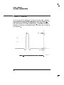
13. How the Instrument Works
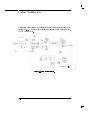
Basics of Sequential Sampling . . . . . . . . . .
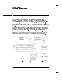
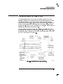
System Architecture . . . . . . . . . . . . . .
The major plug-in module hardware components
The major mainframe hardware components . .
Probe selection . . . . . . . . . . . . . . .
System bandwidth . . . . . . . . . . . . . .
Probe types . . . . . . . . . . . . . . . .
Summary . . . . . . . . . . . . . . . . . .
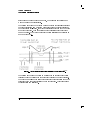
Standard and Enhanced Trigger Modes . . . . . .
DC-2.5 GHz mode . . . . . . . . . . . . . .
DC-100 MHz mode . . . . . . . . . . . . .
2-12 GHz mode (Option 100 only) . . . . . . .
12 GHz/Gate mode (Option 100 only) . . . . .
Index
Contents-10
.
.
.
.
.
.
.
.
.
.
.
.
.
.
.
.
.
.
.
.
.
.
. . .
. . .
.
.
.
.
.
.
.
.
.
.
.
13-3
13-8
13-9
13-10
13-12
13-17
13-18
13-21
13-22
13-22
13-22
13-23
13-25
Figures
0-1.
1-1.
1-2.
1-3.
2-1.
4-1.
4-2.
4-3.
4-4.
4-5.
4-6.
5-1.
5-2.
5-3.
5-4.
5-5.
5-6.
5-7.
5-8.
5-9.
5-10.
5-11.
5-12.
5-13.
5-14.
5-15.
5-16.
5-17.
5-18.
5-19.
5-20.
5-21.
5-22.
5-23.
5-24.
5-25.
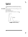
6-1.
Example of a static-safe work station. . . . . . . . . . . .
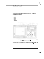
The instrument front panel. . . . . . . . . . . . . . . .
The instrument display. . . . . . . . . . . . . . . . . .
The instrument rear panel. . . . . . . . . . . . . . . . .
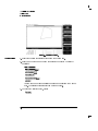
The Help menu. . . . . . . . . . . . . . . . . . . . . .
Current Frame 1Temp condition . . . . . . . . . . . . .
Plug-in calibration menu . . . . . . . . . . . . . . . . .
Oset Zero Calibration . . . . . . . . . . . . . . . . . .
Dark calibration menu . . . . . . . . . . . . . . . . . .
Electrical Channel Calibrate Menu . . . . . . . . . . . . .
External Scale Menu . . . . . . . . . . . . . . . . . . .
Setting up your measurement system. . . . . . . . . . . .
Position of data waveform. . . . . . . . . . . . . . . . .
Extinction ratio measurement. . . . . . . . . . . . . . .
Eye height measurement. . . . . . . . . . . . . . . . .
Crossing percentage measurement. . . . . . . . . . . . .
Eye width measurement. . . . . . . . . . . . . . . . . .
Jitter measurement. . . . . . . . . . . . . . . . . . . .
Duty cycle distortion measurement. . . . . . . . . . . . .
Q-factor measurement. . . . . . . . . . . . . . . . . . .
Rise time measurement. . . . . . . . . . . . . . . . . .
Fall time measurement. . . . . . . . . . . . . . . . . .
Setting up the measurement. . . . . . . . . . . . . . . .
Position of data waveform. . . . . . . . . . . . . . . . .
Eye with a mask. . . . . . . . . . . . . . . . . . . . .
Mask with a 20% margin set. . . . . . . . . . . . . . . .
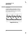
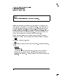
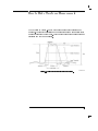
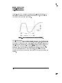
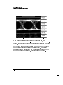
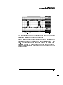
Conventional eye diagram display. . . . . . . . . . . . .
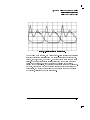
Similar eye diagram in eyeline mode. . . . . . . . . . . .
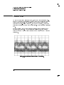
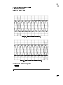
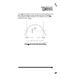
Conventional eye diagram of a low power signal. . . . . . .
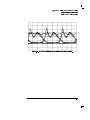
Low power signal viewed with eyeline mode using averaging.
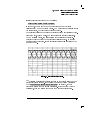
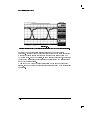
Mask violation and the sequence leading to the violation. . .
Front panel connection for eyeline mode. . . . . . . . . .
Rear panel connection for eyeline mode. . . . . . . . . . .
Display after initial mask alignment. . . . . . . . . . . . .
Display after time base position adjustment. . . . . . . . .
Error trace capture example. . . . . . . . . . . . . . . .
Legal and illegal polygon construction. . . . . . . . . . . .
xv
1-9
1-11
1-15
2-5
4-6
4-11
4-14
4-16
4-18
4-20
5-4
5-5
5-11
5-13
5-14
5-15
5-16
5-17
5-20
5-21
5-23
5-27
5-28
5-32
5-35
5-38
5-39
5-40
5-41
5-42
5-43
5-44
5-50
5-50
5-51
6-12
Contents-11
Contents
6-2.
6-3.
6-4.
6-5.
6-6.
6-7.
6-8.
6-9.
6-10.
6-11.
7-1.
7-2.
7-3.
7-4.
7-5.
7-6.
7-7.
7-8.
7-9.
7-10.
9-1.
9-2.
9-3.
9-4.
9-5.
9-6.
9-7.
9-8.
9-9.
10-1.
10-2.
10-3.
10-4.
10-5.
11-1.
11-2.
11-3.
11-4.
11-5.
Dening a polygon. . . . . . . . . . . . . . . . . . . .
Rescaling a polygon. . . . . . . . . . . . . . . . . . . .
Mask with a 15% margin. . . . . . . . . . . . . . . . .
Extinction ratio measurement. . . . . . . . . . . . . . .
Eye height measurement. . . . . . . . . . . . . . . . .
Crossing % measurement. . . . . . . . . . . . . . . . .
Eye width measurement. . . . . . . . . . . . . . . . . .
Jitter measurement. . . . . . . . . . . . . . . . . . . .
Duty cycle distortion measurement. . . . . . . . . . . . .
Measuring Q-factor. . . . . . . . . . . . . . . . . . . .
Pulse parameters the instrument measures. . . . . . . . .
The instrument uses this process for waveform measurement.
Some measurements are made from the histogram. . . . . .
The middle 20 percent of the waveform is ignored. . . . . .
Calculating the 10, 50, and 90 percent thresholds. . . . . .
Thresholds are used to determine edges. . . . . . . . . . .
The system ignores incomplete transitions when dening
edges. . . . . . . . . . . . . . . . . . . . . . . . .
Waveform period is measured at the middle threshold. . . .
Waveform denitions used to make voltage measurements. . .
You may dene 1time. . . . . . . . . . . . . . . . . . .
Erroneous rise time measurements due to jitter. . . . . . .
Eect of vertical dc errors on measurement accuracy. . . . .
Edges of opposite polarity reinforce dc errors. . . . . . . .
Faster transitions decrease eect of dc oset errors. . . . . .
Measure time intervals at fastest-changing part of transition. .
Narrow pulse applied to the instrument. . . . . . . . . . .
Errors in pulse height measurement. . . . . . . . . . . .
Error in pulse width at 10% level is approximately equal to
the error in 10%{90% rise time. . . . . . . . . . . . .
Eect of probe capacitance. . . . . . . . . . . . . . . . .
Standard measurement thresholds. . . . . . . . . . . . .
Standard deviations of a Gaussian distribution. . . . . . . .
Sine wave in the frequency domain. . . . . . . . . . . . .
An FFT display. . . . . . . . . . . . . . . . . . . . . .
An example of the histogram display. . . . . . . . . . . .
The Directory display. . . . . . . . . . . . . . . . . . .
Dots only. . . . . . . . . . . . . . . . . . . . . . . .
Connected dots. . . . . . . . . . . . . . . . . . . . . .
Screen in grid mode using one graph. . . . . . . . . . . .
Screen in frame mode using one graph. . . . . . . . . . .
Contents-12
6-15
6-16
6-17
6-33
6-35
6-37
6-38
6-39
6-40
6-42
7-3
7-5
7-6
7-8
7-10
7-11
7-12
7-13
7-15
7-19
9-8
9-10
9-11
9-12
9-12
9-16
9-17
9-18
9-19
10-8
10-20
10-29
10-30
10-38
11-4
11-28
11-29
11-31
11-32
Contents
11-6.
11-7.
11-8.
11-9.
11-10.
11-11.
11-12.
11-13.
13-1.
13-2.
13-3.
13-4.
13-5.
13-6.
13-7.
13-8.
13-9.
13-10.
13-11.
13-12.
13-13.
13-14.
13-15.
13-16.
13-17.
13-18.
13-19.
13-20.
Screen in frame mode using two graphs. . . . . . . . . . .
A functional view of the limit test. . . . . . . . . . . . .
Setup Print screen. . . . . . . . . . . . . . . . . . . .
The System Conguration display. . . . . . . . . . . . . .
A typical Cal Status display. . . . . . . . . . . . . . . .
A typical Firmware support screen. . . . . . . . . . . . .
Storing a waveform. . . . . . . . . . . . . . . . . . . .
Saving to pixel memory. . . . . . . . . . . . . . . . . .
The sampling circuit. . . . . . . . . . . . . . . . . . .
Sequential sampling process. . . . . . . . . . . . . . . .
Acquisition with record length = 64. . . . . . . . . . . .
Acquisition with record length = 2250. . . . . . . . . . .
Hardware block diagram. . . . . . . . . . . . . . . . . .
The probe is a part of the circuit under test. . . . . . . . .
Simplied equivalent circuit of DUT and probe. . . . . . . .
Reduced amplitude and dc oset caused by probe loading. . .
Eects of probe capacitance. . . . . . . . . . . . . . . .
Resistive divider probe. . . . . . . . . . . . . . . . . .
Active probe. . . . . . . . . . . . . . . . . . . . . . .
Viewing a 10 Gb/s eye diagram using 12 GHz trigger. . . . .
12 GHz mode jitter with 200 mV p-p sine wave input. . . . .
12 GHz/Gate mode jitter with 300 mV p-p sine wave input. .
Gating application. . . . . . . . . . . . . . . . . . . .
2.5 GHz trigger on signal with pulsed 2 GHz RF content. . .
12 GHz trigger on signal with pulsed 10 GHz RF content. . .
10 Gb/s digital eye diagram without gating. . . . . . . . .
10 Gb/s digital eye diagram with a 1ms gating pulse. . . . .
Result of triggering the low speed gating pulse generator from
the 10 Gb/s pattern generator. . . . . . . . . . . . . .
11-33
11-43
11-71
11-80
11-86
11-89
11-94
11-97
13-3
13-5
13-6
13-7
13-8
13-12
13-13
13-14
13-15
13-18
13-20
13-24
13-26
13-27
13-28
13-29
13-29
13-30
13-31
13-32
Contents-13
Tables
0-1.
4-1.
4-2.
4-3.
4-4.
9-1.
11-1.
Static-Safe Accessories . . . . . . . . . . . . . . . .
Factory Calibration Summary . . . . . . . . . . . . .
Optical and Electrical Channel User Calibration Summary
Miscellaneous User Calibration Summary . . . . . . . .
Complete Calibration Summary . . . . . . . . . . . .
Rise-Time Measurement Errors . . . . . . . . . . . .
Partial listing of the Text Verbose Format for a Normal
Waveform . . . . . . . . . . . . . . . . . . . .
11-2. Partial Example of the Text Y Values Format . . . . . .
11-3. Default Setups . . . . . . . . . . . . . . . . . . .
Contents-14
.
.
.
.
.
.
. xvi
. 4-4
. 4-9
. 4-10
. 4-21
. 9-15
. . 11-16
. . 11-20
. . 11-67
1
The Instrument at a
Glance
The Instrument at a Glance
What you'll nd in this chapter
This chapter provides you with a brief overview of how the instrument functions, descriptions of the
front and rear panels, and a description of the key conventions used in this manual. The following
topics are discussed:
options and accessories
menu and key conventions
the front panel and rear panel
the display
indicator lights
entry devices
keys that do not display menus on screen
Understanding the information in this chapter will help you operate the instrument. Information on
using the front-panel interface is in the User's Quick Start Guide supplied with the instrument.
1-2
The Agilent 83480A-series digital communications analyzer and Agilent
54750A-series digitizing oscilloscopes are powerful and versatile instruments
designed for use in research, development, production and evaluation testing
in the telecommunication, data communication, RF/microwave and signal
integrity areas. Data acquisition and measurement analysis are performed
in parallel, enabling the instrument to achieve outstanding measurement
throughput. The instrument provides fast, repeatable communications
waveform performance analysis with automated pulse and eye diagram
statistical measurements. Optical or electrical conformance tests to both
user-dened and industry standard eye diagram masks or pulse templates are
eciently executed. The instrument is a modular platform which accepts up
to two dual-channel electrical or optical measurement modules.
The instrument provides you with the necessary capabilities to test and
measure analog and digital circuits. The instrument provides:
Optical and electrical measurement channels (Agilent 83480A only)
Optical input wavelength:
750 nm to 860 nm (Agilent 83480A, with an Agilent 83487A only)
1000 nm to 1600 nm for (Agilent 83480A, with an Agilent 83486A)
1200 to 1600 nm for (Agilent 83480A, with an Agilent 83485A)
Integrated average optical power meter (Agilent 83480A, with any optical
module)
Calibrated vertical watts scale (Agilent 83480A, with any optical module)
Up to 50 GHz bandwidth
TDR/TDT measurements (Agilent 54750A only, or Agilent 83480A with
Agilent 54755A option)
This function available with rmware revision A.02.00 and above.
1-3
The Instrument at a Glance
Standard masks and templates, (Agilent 83480A only) including:
Optical Masks
STM0/OC1
STM1/OC3
OC12
OC24
STM16/OC48
FC133
FC266
FC531
FC1063
FDDI
100BASE-FX
GIGABIT ETHERNET
Electrical Masks
STS1 Eye
STS1 Pulse
STS3 Eye
STS3 Pulse 0
STS3 Pulse 1
DS1
DS1C
DS2
DS3
PDH 2.048 Mb
PDH 8.448 Mb
PDH 34.4 Mb
PDH 139 Mb 0
PDH 139 Mb 1
Automatic mask and template scaling, positioning, and testing
Statistical waveform analysis
FFT
1-4
Ordering Information
Supplied accessories
Optional accessories
Power cord for country of destination
Agilent 83480A, 54750A Quick Start Guide
Agilent 83480A, 54750A User's Guide
Agilent 83480A, 54750A Programmer's Quick Reference
Agilent 83480A, 54750A Programmer's Guide
9300-1484 ESD kit
One year warranty
Option 001 Agilent 83480A only. Agilent Eyeline Mode software. Loads
downloadable eyeline analysis program directly to the
internal disk drive. Enables Eyeline Mode operation with
an Agilent 71603B, Agilent 71612A (Agilent 70843A) error
performance analyzer or Agilent 71604B pattern generator.
Option 100 Provides direct triggering on 12 GHz signals. An external
gating signal can be used to further extend the triggering
capabilities.
Option 908 Rackmount kit, without handles, Agilent p/n 54710-68704
Option 909 Rackmount kit, for instruments with handles, Agilent p/n
54710-68705
Option 0BW Service guide
Option 0B1 Additional set of user documentation
Option 0B0 Deletes the user documentation
Option UK6 Measured performance data
Agilent 10086A ECL terminator
Agilent 11898A extender module
Agilent 54006A 6 GHz divider probe
Agilent 54008A 22 ns delay line
Agilent 54118A 500 MHz to 18 GHz trigger
Agilent 54753A TDR plug-in module
Agilent 54754A TDR plug-in module
Agilent 54755A TDR rmware kit (for use with the Agilent 83480A)
1-5
The Instrument at a Glance
Ordering Information
Agilent 83480K communications rmware kit (for use with the Agilent
54750A)
Agilent 83482A 40 GHz optical/electrical plug-in module
Agilent 83483A, 54751A electrical plug-in module
Agilent 83484A, 54752A 50 GHz electrical plug-in module
Agilent 83485A optical/electrical plug-in module
Agilent 83485B high speed optical/electrical plug-in module
Agilent 83486A 1300-1500 nm multimode optical/electrical plug-in module
Agilent 83487A 850 nm multimode optical/electrical plug-in module
Blank, one (1) slot ller plug-in, Agilent part number 54700-68702 or
Agilent 54700B
Connection devices
SMA (f-f) adapter, Agilent part number 1250-1158
APC 3.5 (f-f) adapter, Agilent part number 1250-1749
1-6
Menu and Key Conventions
The keys labeled Trigger, Disk, and Run are all examples of front-panel keys.
Pressing some front-panel keys accesses menus of functions that are displayed
along the right side of the display screen. These menus are called softkey
menus.
Softkey menus list functions other than those accessed directly by the
front-panel keys. To activate a function on the softkey menu, press the
unlabeled key immediately next to the annotation on the screen. The
unlabeled keys next to the annotation on the display are called softkeys.
Additional functions are listed in blue type above and below some of the
front-panel keys. These functions are called shifted functions. To activate a
shifted function, press the blue front-panel Shift key and the front-panel key
next to the desired function.
Throughout this manual front-panel keys are indicated by a box around
the key label, for example, 4Timebase5. Softkeys are indicated by shading on
the key label, for example, Scale . The softkeys displayed depend on the
front-panel key pressed and which menu is selected. Shifted functions are
indicated by the front-panel 4Shift5 key ( blue key) followed by the shaded
shifted function, for example the Local function (above the 4Stop/Single5
front-panel key) will be shown as 4Shift5, 4Local5.
A softkey with On and O in its label can be used to turn the softkey's
function on or o. To turn the function on, press the softkey so On is
highlighted. To turn the function o, press the softkey so O is highlighted.
An On or O softkey function will be indicated throughout this manual as:
Test On.
NNNNNNNNNNNNNNNNN
NNNNNNNNNNNNNN
1-7
The Instrument at a Glance
Menu and Key Conventions
A softkey such as Sweep Triggered Freerun oers you a choice of
functions. In this case you could choose Triggered by pressing the softkey
until Triggered is highlighted, or choose Freerun by pressing the softkey until
Freerun is highlighted. A choices softkey will be indicated throughout this
manual as: Sweep Triggered Freerun Triggered.
NNNNNNNNNNNNNNNNNNNNNNNNNNNNNNNNNNNNNNNNNNNNNNNNNNNNNNNNNNNNNNNNNNNNNNN
NNNNNNNNNNNNNNNNNNNNNNNNNNNNNNNNNNNNNNNNNNNNNNNNNNNNNNNNNNNNNNNNNNNNNNN
When some softkeys, such as Eye Height , are pressed the rst time, a
measurement will be made and the result will be provided. Some softkeys,
such as Offset require the entry of a numeric value. To enter or change the
value, use the general purpose knob located below the front-panel Measure
section.
NNNNNNNNNNNNNNNNNNNNNNNNNNNNNNNN
NNNNNNNNNNNNNNNNNNNN
1-8
The Front Panel
The front panel of the instrument includes a display area and several
functional areas, including:
Control
Measure
Setup
Storage
System
Autoscale
Figure 1-1. The instrument front panel.
The display area and Autoscale key are described in this chapter. Information
on the other functional areas are included later in this manual.
1-9
The Instrument at a Glance
The Front Panel
4Autoscale5
The Autoscale key causes the instrument to quickly analyze the signal. Then,
it sets up the vertical, horizontal, and trigger to best display that signal.
Autoscale can nd:
Repetitive signals with:
frequency
50 Hz
duty cycle
>1%
amplitude
10 mV p-p or 120 Wp-p (optical signals only on the
Agilent 83480A, 83485A)
trigger amplitude >20 mV
Autoscale looks for signals on all channels, even if they are turned o. It also
searches for a trigger signal on the external trigger inputs.
Agilent 83480A Option 100 only: If no trigger signal is detected at the
external input, and the instrument is in the 2.5 GHz trigger mode, the sweep
will stop. If the instrument is in the 12 GHz trigger mode, it will sweep
continuously in \freerun" condition.
If the Autoscale key is pressed unintentionally, use the Undo Autoscale
function to return the instrument to the settings that existed prior to pressing
the Autoscale key. To undo an Autoscale function press:
4Shift5, Undo Autoscale
To quickly rescale the vertical axis, without altering the timebase, press:
4Channel5
Channel Autoscale (only on Agilent 83480A, 83483A, 83485A)
NNNNNNNNNNNNNNNNNNNNNNNNNNNNNNNNNNNNNNNNNNNN
NNNNNNNNNNNNNNNNNNNNNNNNNNNNNNNNNNNNNNNNNNNNNNNNNNNNN
1-10
The Instrument at a Glance
The Front Panel
Display
The instrument has a high-resolution, color display. The display is divided
into several areas as shown in Figure 1-2.
Figure 1-2. The instrument display.
1-11
The Instrument at a Glance
The Front Panel
Status area
The Status area displays prompts, messages, error messages, warnings, and
the number of averages when averaging is turned on.
Graticule area
The Graticule area is also referred to as the waveform viewing area. This is
where all the waveform data and markers are displayed on the screen.
Time Base area
The Time Base area lists the time base scale setting, reference location,
and position setting. The reference location is indicated by an arrow. In
Figure 1-2, the time base settings are:
Scale : : : : : : : : : : : : : : : : : : : : : : : : : : : : : : : : : : : : : : : : : : : : : : : : : : : : : : : : : : : : : 5.0 ns/div
Reference location : : : : : : : : : : : : : : : : : : : : : : : set to the left of the graticule area
Position : : : : : : : : : : : : : : : : : : : : : : : : : : : : : : : : : : : : : : : : : : : : : : : : : : : : : : : : : : : : : : : 20 ns
Channel Settings and Channel Settings and Measurement Results share the same area. Channel
Measurement Results Settings are displayed only when the measurements are o. When making
an automatic measurement, the results are displayed in place of the channel
area
settings.
To display the Channel Settings, press:
4Shift5 Clr Meas
When a channel number is displayed, it indicates the channel is turned on.
In Figure 1-2, the channel settings are:
Channel 1, on
Scale : : : : : : : : : : : : : : : : : : : : : : : : : : : : : : : : : : : : : : : : : : : : : : : : : : : : : : : : : : 75 mV/div
Oset : : : : : : : : : : : : : : : : : : : : : : : : : : : : : : : : : : : : : : : : : : : : : : : : : : : : : : : : : : : 010 mV
Channel 2, on
Scale : : : : : : : : : : : : : : : : : : : : : : : : : : : : : : : : : : : : : : : : : : : : : : : : : : : : : : : : : : 60 mV/div
Oset : : : : : : : : : : : : : : : : : : : : : : : : : : : : : : : : : : : : : : : : : : : : : : : : : : : : : : : : : : : : : : 0 mV
Channels 3 and 4, o
NNNNNNNNNNNNNNNNNNNNNNNNNN
Marker Results and Statistics Results share the same area. Statistics Results
Marker Results and
Statistics Results area are displayed only when the manual and waveform markers are turned o, or
when the measurement marker readout is turned o.
1-12
The Instrument at a Glance
The Front Panel
Histogram, Limit Test
and Mask Test
The entire area below the timebase area is used by the Histogram, Limit Test
and Mask Test features while in their respective menus.
Softkey menu area
Softkey menus are displayed in this area. The menu that is displayed
depends on which key is pressed. The Agilent 83480A, 54750A Quick Start
Guide contains an explanation of how the softkeys operate.
Memory bar
The memory bar represents the entire waveform record. The highlighted part
of the memory bar represents the portion of the waveform record currently
on the display. When possible, the acquisition hardware is set up so all of the
waveform record is displayed on the screen. When the acquisition is stopped
and the waveform is magnied with the time base controls, the memory bar
indicates which portion of the waveform is viewed.
Entry devices
The entry devices are:
the knob
the arrow keys
the keypad
You can use the entry devices to change the numeric settings of some
softkeys, such as trigger level, or to select an item from a list of choices.
When using the entry devices to scroll through a list of choices, you may
notice the background color of each item change as you scroll through the
list. Occasionally, a particular feature may not be available. In this case, the
background color of that feature will not change as you scroll through the list.
1-13
The Instrument at a Glance
The Front Panel
Indicator lights
There are three indicator lights near the top-left corner of the instrument.
These lights give you a quick indication of the acquisition status of the
instrument.
Armed
When the armed light is on, it indicates the trigger circuit is armed and
waiting for a valid trigger event to occur. A valid trigger event occurs when a
signal meets the triggering conditions specied in the trigger menu.
Triggered
When the triggered light is on, it indicates the instrument accepted a trigger
event. Every time the instrument accepts a trigger event, one data point is
sampled. When enough points have been sampled to ll the record length, a
trace is completed.
The triggered light can be used to help determine the trigger thresholds. To
do this, simply move the trigger level in either direction. When the triggered
light turns o, you know that is one of the trigger thresholds. Move the
trigger level in the other direction to determine the other threshold. You now
know what the trigger thresholds are and you can set the trigger level as
required by your application.
Typically the trigger level is set halfway between the two thresholds.
Freerun
Freerun automatically provides a trigger as soon as the trigger is armed. It is
used to view the input signal when no valid triggers are available.
Agilent 83480A Option 100 only: When in the 12 GHz mode, the triggered
and freerun lights are illuminated at all times to reect the operation of the
12 GHz trigger.
1-14
The Rear Panel
Figure 1-3. The instrument rear panel.
1-15
The Instrument at a Glance
The Rear Panel
Line Input
The Line Input is the input for the line power source. Make sure the
line-power source outlet has a protective ground contact.
Line On/O
The Line switch turns the instrument on and o. After applying power, allow
the temperature of the instrument to stabilize for best measurement results.
NOTE
The instrument continues to draw power when it is plugged into the ac power source, even if the line
power switch is o.
Fuse
The power input fuse is located behind a small removable metal plate.
Depending on the voltage of the line power, the line-power fuse can be
replaced with one of the following values:
100V operation: F15A, 250V : : : : : : : : : : : : : : Agilent part number 2110-0054
120V operation: F12A, 250V : : : : : : : : : : : : : : Agilent part number 2110-0249
240V operation: F8A, 250V : : : : : : : : : : : : : : : Agilent part number 2110-0342
Line Select
The Line Select switch adapts the instrument to the power source. Select
either 115 V or 230 V, whichever most closely matches the voltage being
supplied to the Line Input. To change Line Select, remove the black plastic
insert, rotate clockwise 180 , and reinsert it.
Before switching on this instrument, make sure that the line voltage selector
switch is set to the voltage of the power supply and the correct fuse is
installed. Assure the supply voltage is in the specied range.
CAUTION
GPIB
The GPIB connector allows an external computer to communicate with the
instrument.
1-16
The Instrument at a Glance
Parallel
Printer Port
The Parallel Printer Port allows the instrument to communicate with remote
printers or plotters.
High Speed Data Port
Not used.
Degauss
Activates a CRT screen degaussing.
+15 V, 150 mA output The +15 V, 150 mA output provides power for external modules, such as the
Agilent 54118A 18 GHz trigger.
Opt 100 Trigger Gate
This TTL compatible input allows gating of the 12 GHKz trigger. Refer to
\2-12 GHz mode (Option 100 only)" in Chapter 13 for additional information.
Memory Protect
Frame Cal protected
Best cal protected
Forces system ROM
programming at
power-up
Forces boot ROM
programming
Up position prevents timebase calibration from
being overwritten; switch to down position to
perform mainframe calibration.
Not used.
In down position, the operating system will be
loaded from the disk in the disk drive at power-up
(approximately 7 minutes).
Leave in up position (factory use only).
1-17
The Instrument at a Glance
2
General Purpose Keys
General Purpose Keys
What you'll nd in this chapter
The front panel includes the following functions:
the
the
the
the
the
the
Clear Display key
Fine function
Help key
Local key
Run key
Stop/Single key
This chapter describes each of these functions. They are listed alphabetically.
2-2
The Clear Display Key
The Clear Display key erases all channel and function waveform data from
the graticule area, and resets all associated measurements and measurement
statistics.
When the instrument is If the instrument is stopped, the display remains cleared of waveform data
until the trigger circuit is rearmed and the instrument is triggered. Then, the
stopped
new data is displayed and measurements are recalculated.
When the instrument is If the instrument is running, new waveform data is displayed on the next
acquisition and all measurements are recalculated.
running
2-3
The Fine Function
llllllllllllllllllll
The Fine function increases the resolution of the knob used to adjust the
channel scale, oset, and time base scale. For example, on most plug-ins the
knob changes the channel scale in a 1-2-5 sequence, such as 10 mV, 20 mV,
and 50 mV.
When the Fine function is selected, the knob changes the channel scale in
smaller increments, such as 10.0 mV, 10.1 mV, 10.2 mV.
To put the instrument in the Fine mode, press:
4Shift5 Fine
Repeat the process to exit the Fine mode.
The screen displays the word FINE at the top-right corner of the graticule
area when the Fine mode is active.
NNNNNNNNNNNNNN
2-4
The Help Key
The Help key assists you in nding the key sequence used to execute a
particular feature. When Help is pressed, a three-column index is displayed
on the screen.
The left column lists the features of the instrument.
The middle column lists the hardkeys.
The right column lists the softkeys.
Use either the knob or arrow keys to scroll through the list of features.
Figure 2-1. The Help menu.
For example, to move a signal vertically on the display, look up Channel
vertical scale in the Help menu list. The middle column instructs you to press
the Channel key, and the right column instructs you to press the Scale key.
Features may be listed under dierent names. For example, you could have
also looked for scale, vertical or vertical scale. Each of these titles give you
the same key sequence to follow.
2-5
The Local Key
To access the Local function, press:
4Shift5 4Local5
The Local function returns control of the instrument to the front panel. This
is the only key that is active when the instrument is under remote control.
The exception occurs when the controller sends a Local Lockout command.
The Local Lockout command disables the Local function key.
2-6
The Run Key
The Run key causes the instrument to resume acquiring data. If the
instrument is stopped, it starts acquiring data on the next trigger event. If
the instrument is already in the Run mode, it continues to acquire data on
successive trigger events.
If pressing the Run key does not cause waveform data to display on the
screen, try the following:
Press the Autoscale key.
Make sure a signal is connected to one of the channels and the display for
that channel is turned on.
Make sure the oset does not have the trace clipped o the display.
Check the trigger setup conditions to make sure the trigger conditions are
valid for the signal.
Set the Trigger Sweep mode to Freerun. Freerun forces the instrument to
trigger, which may allow you to see enough of the signal so that you can
set up the front panel properly.
2-7
The Stop/Single Key
Pressing the Stop/Single key causes the instrument to stop acquiring data.
The status area of the screen displays the message:
Acquisition is stopped.
Each subsequent press of the Stop/Single key rearms the trigger circuit. A
complete acquisition cycle is performed, any measurements are recalculated,
and the status area of the screen displays the message:
Acquisition is complete.
If all of the channels are turned o or if a trigger event is not found, the
instrument will not acquire any data.
2-8
3
Specications and
Characteristics
Specications and Characteristics
What you'll nd in this chapter
This chapter lists specications and characteristics for the Agilent 83480A digital communications
analyzer and the Agilent 54750A digitizing oscilloscope. Specications apply over the temperature range
+15 C to +35 C (unless otherwise noted) after the instrument's temperature has been stabilized after
60 minutes of continuous operation.
Specications
Specications described warranted performance.
Characteristics
Characteristics provide useful, nonwarranted information about the functions and performance of the
instrument. Characteristics are printed in italics.
Calibration Cycle
Agilent Technologies warrants instrument specications over the recommended calibration interval. To
maintain specications, periodic recalibrations are necessary. We recommend that the Agilent 83480A
be calibrated at an Agilent Technologies service facility every 24 months.
Additional specications and characteristics are included in the user's guides for the individual plug-in
modules.
3-2
Horizontal System
Scale factor
Full scale is ten divisions.
Minimum : : : : : : : : : : : : : : : : : : : : : : : : : : : : : : : : : : : : : : : : : : : : : : : : : : : : : : : : : 10 ps/div
Maximum : : : : : : : : : : : : : : : : : : : : : : : : : : : : : : : : : : : : : : : : : : : : : : : : : : : : : : : : : : : 1 s/div
Delay
Time oset relative to trigger.
Minimum : : : : : : : : : : : : : : : : : : : : : : : : : : : : : : : : : : : : : : : : : : : : : : : : : : : : : : : : : : : : : 22 ns
Maximum : : : : : : : : : : : : : 1000 screen diameters or 10 s, whichever is smaller
Time interval accuracy
8 ps 60.1% of reading (dual marker measurement)
Time interval resolution
(screen diameter)/(record length) or 62.5 fs, whichever is larger
Time display resolution
451 points horizontally
3-3
Trigger Specications
Electrical and Optical Channels
Standard instrument, 2.5 GHz mode
Trigger bandwidth
dc 0 2.5 GHz
Sensitivity
40 mV p-p at 100 MHz, increasing linearly to 200 mV p-p at 2.5 GHz.
Pulse width
200 ps >200 mV
Bandwidth limit
Trigger bandwidth reduced to approximately 100 MHz with bandwidth limit
enabled.
Maximum trigger signal 62 Vdc + ac peak (+16 dBm)
Jitter
2.5 ps rms + 5E-5 2 delay setting (at 2.5 GHz with 200 mV source).
3-4
Specications and Characteristics
Trigger Specications
Electrical and Optical Channels
Option 100, 12 GHz mode
For more information on Option 100 triggering, refer to Chapter 13.
Trigger bandwidth
2.0 GHz 0 12 GHz (1 GHz to 15 GHz typical)
Sensitivity
200 mV p-p from 2.0 GHz to 12 GHz (sine wave input)
Maximum trigger signal 62 Vdc + ac peak (+16 dBm)
Jitter
< 2 ps rms with time delay less than 100 ns
Option 100, 12 GHz/Gate mode
For more information on Option 100 triggering, refer to Chapter 13.
Trigger bandwidth
2.0 GHz 0 12 GHz (typical)
Sensitivity
300 mV p-p from 2.0 GHz to 12 GHz (sine wave input) (typical)
Trigger gating levels
(characteristic)
Standard TTL:
Disable : : : : : : : : : : : : : : : : : : : : : : : : : : : : : : : : : : : : : : : : : : : : : : : : : : : : : : : : : : : : : <0.8 V
Enable : : : : : : : : : : : : : : : : : : : : : : : : : : : : : : : : : : : : : : : : : : : : : : : : : : : : : : : : : : : : : : >2.0 V
Maximum allowable range : : : : : : : : : : : : : : : : : : : : : : : : : : : : : : : : : : : : 0.0 V|5.0 V
<1 MHz gating rate input impedance : : : : : : : : : : : : : : : : : : : : : : : : high (10 k
)
3-5
General Specications
Use
Indoor
Temperature
Operating : : : : : : : : : : : : : : : : : : : : : : : : : : : : : : : : : 15 C to +35 C (59 F to +95 F)
Non-operating : : : : : : : : : : : : : : : : : : : : : : : : 040 C to +70 C (040 F to +158 F)
Humidity
NOTE
This test requires a one hour warm-up period.
Operating : : : : : : : up to 95% humidity (non-condensing) at +35 C (+95 F)
Non-operating : : : : : : : : : : : up to 90% relative humidity at +65 C (+149 F)
Altitude
Operating : : : : : : : : : : : : : : : : : : : : : : : : : : : : : : : : : : : : up to 4,600 meters (15,000 ft)
Non-operating : : : : : : : : : : : : : : : : : : : : : : : : : : : : : : up to 15,300 meters (50,000 ft)
Vibration
Operating
Random vibration 50500 Hz, 10 minutes per axis, 0.3 grms
Non-operating
Random vibration 50500 Hz, 10 minutes per axis, 2.41 grms ; Resonant
search, 5 to 500 Hz swept sine, 1 octave/minute sweep rate, 0.75g,
5 minute resonant dwell at 4 resonances per axis.
3-6
Specications and Characteristics
Power Requirements
Voltage : : : : : : : : : : : : : : : : : : : : : : : : : : : : : : 90 to 132 or 198 to 264 Vac, 48-66 Hz
Power : : : : : : : : : : : : : : : : : : : : : : : : : : : : : : : : : : : : : : : : : : : : : : : : : : : : : : 1200 VA; 650 W
Weight (approximate)
Net : : : : : : : : : : : : : : : : : : : : : : : : : : : : : : : : : : : : : : : : : : : : : : : : : : : : : : : : : : 24.5 kg (54 lb)
Shipping : : : : : : : : : : : : : : : : : : : : : : : : : : : : : : : : : : : : : : : : : : : : : : : : : : : : 31.8 kg (70 lb)
Dimensions
H2W2D
238.2 mm 2 433.6 mm 2 637.38 mm
(9.378 in 2 17.071 in 2 25.094 in)
3-7
Specications and Characteristics
4
Calibration Overview
Calibration Overview
CAUTION
This chapter describes the calibration of the mainframe and the plug-in
modules. It is intended to give you, or the calibration laboratory personnel,
an understanding of the various calibration procedures available, and how
they were intended to be used. There is a description of the calibration menu
included in the manuals provided with the plug-in modules and probes.
Proper calibration is critical to measurement accuracy and repeatability. The
Agilent 54750A/83480A and their associated modules and accessories require
that both factory and user calibrations be implemented at the recommended
intervals in order to perform measurements at their published specications.
This chapter is divided into three sections. The rst section describes
factory calibrations. A factory calibration consists of verifying instrument
performance to all specications. If an instrument fails to meet specications,
adjustment or repair may be necessary. For most users, this will mean
shipping the instrument back to an authorized service center. Some users
may purchase the required instrumentation and perform the factory timebase
calibrations themselves using the optional Agilent 83480A, 54750A Service
Guide.
The second part of the chapter addresses calibrations that are routinely
performed by the end user. Subsections in each of the two main sections
discuss the individual calibrations. In addition, there will be summary tables
at the end of each of these sections summarizing the main areas addressed.
A complete calibration summary table is included at the end of the chapter.
Both factory and user calibrations must be performed regularly in order to
ensure proper measurement accuracy and repeatability.
The input circuits can be damaged by electrostatic discharge (ESD). Avoid
applying static discharges to the front-panel input connectors. Before
connecting a coaxial cable to the connectors, momentarily short the center
and outer connectors of the cable together. Avoid touching the front panel
input connectors without rst touching the frame of the instrument. Be sure
that the instrument is properly earth-grounded to prevent buildup of static
charge. It is strongly recommended that an antistatic mat and wristband be
used when connecting to electrical channel inputs, particularly TDR inputs.
4-2
Calibration Overview
Calibration interval
Agilent Technologies recommends that the factory calibration be performed
on a periodic basis. Agilent Technologies designs instruments to meet
specications over the recommended calibration interval provided that the
instrument is operated within the specied operating environment. To
maintain specications, periodic recalibrations are necessary. We recommend
that the plug-in module be calibrated at an Agilent Technologies service
facility every 12 months. Users are encouraged to adjust the calibration cycle
based on their particular operating environment or measurement accuracy
needs.
Required warm-up time The instrument requires a 1 hour warm-up period before any of the
calibrations mentioned in this chapter are performed. It is not enough for the
instrument to be in the standby setting. It must be turned on and running for
the entire hour.
Remote operation
Contents
Remote programming commands for calibrations are included in the Agilent
83480A/Agilent 54750A Programming's Guide. Performing calibrations
remotely is slightly dierent than the operation of front-panel calibrations.
Factory Calibrations on page 4-4
User Calibrations|Optical and Electrical on page 4-7
Complete Calibration Summary on page 4-20
4-3
Factory Calibrations
The following calibrations are performed at the factory:
Mainframe Calibration
O/E Factory Wavelength Calibration
Table 4-1. Factory Calibration Summary
Calibration
Mainframe Calibration
O/E Factory Wavelength
Calibration
1
What is calibrated
Accuracy and
continuity of the
timescale
The photodetector
responsivity
Measurements
Aected
Recommended
Interval
Softkey Path
Annually at Agilent 4Utility5
Technologies service Calibrate
center or if operating Calibrate frame
temp has changed
and remains 5 C or
more from calibration
temperature. See
service manual.
Not user accessible.1
Channels aected: Annual factory
optical. Amplitude re-calibration of
accuracy of all optical standard wavelengths.
channel
measurements.
Optical power meter
accuracy.
Channels aected:
optical & electrical.
All time base
measurements such
as rise time, fall time,
eye width, and jitter.
FFFFFFFFFFFFFFFFFFFFFFFFFF
FFFFFFFFFFFFFFFFFFFFFFFFFFFFFFFFFFFFFFFFFFF
Refer to \O/E User-Wavelength Calibration" in this chapter.
Mainframe Calibration
Mainframe calibration aects both optical and electrical measurements.
Mainframe calibration improves timebase accuracy. All timebase
measurements such as rise time, fall time, eye width, jitter, and so forth are
aected by the timebase accuracy.
4-4
Calibration Overview
Factory Calibrations
CAUTION
The calibration factors are stored in the nonvolatile RAM of the instrument.
There is a switch on the back panel of the instrument that allows the
mainframe calibration to be protected or unprotected. Next to the switch
there is a drawing that shows each switch's function and protected position.
Refer to the optional Agilent 83480A, 54750A Service Guide for more details
about the mainframe calibration, and the position of the rear-panel memory
protect switches.
To prevent access to the mainframe calibration switch, place a sticker over
the access hole to this switch.
CAUTION
Do not attempt a Mainframe calibration without consulting the Agilent
83480A, 54750A Service Guide.
A mainframe calibration should be performed on a periodic basis, annually,
or when the ambient operating has changed by and remains 5 C dierent
than the operating temperature at which the last mainframe calibration was
performed. To see how much the operating temperature has changed since
the last mainframe calibration and the date of the last mainframe calibration,
check the Calibration status by pressing the following key sequence: 4Utility5,
Calibrate , and then Cal status on.
The temperature change is displayed at the top of the display as shown in the
following gure.
NNNNNNNNNNNNNNNNNNNNNNNNNNNNN
NNNNNNNNNNNNNNNNNNNNNNNNNNNNNNNN
4-5
Calibration Overview
Factory Calibrations
Figure 4-1. Current Frame 1Temp condition
If the Current Frame 1Temp listing is greater than 65 C, then the
mainframe should either be calibrated at the current operating temperature or
be placed in an ambient air temperature that is within 5 C of the temperature
of the current calibration.
O/E Factory Wavelength Calibration
Optical/electrical (O/E) factory wavelength calibration, compensates for the
photodetector responsivity. The accuracy of all optical channel measurements
is dependent on proper O/E calibration. O/E calibrations should be performed
annually. Most customers return their optical plug-ins to an authorized
Agilent Technologies service center for this calibration at the same time they
are having their mainframes re-calibrated.
The Agilent 83480-series optical modules have one or two standard
wavelengths (850 nm or 1310/1550 nm). The O/E Calibration function
allows you to calibrate the instrument for use at one additional user-dened
wavelength. This calibration does not aect the factory calibrations. See
4-6
Calibration Overview
Factory Calibrations
the following section on User Calibrations for additional information on this
procedure.
4-7
User Calibrations|Optical and Electrical
The following calibrations can be performed by the user:
O/E User Wavelength Calibration
Plug-in Module Vertical Calibration
Oset Zero Calibration
Dark Calibration
Probe Calibration
Channel Skew
External Scale
Electrical channels have calibration procedures for:
adjusting timebase skew, for matching propagation delay between channels,
probes, cables, and so forth
using external probes
Optical channels have calibration procedures for:
adjusting timebase skew
monitoring and adjusting internal osets
performing a user-dened O/E responsivity adjustment
CAUTION
The input circuits can be damaged by electrostatic discharge (ESD). Avoid
applying static discharges to the front panel input connectors. Before
connecting a coaxial cable to the connectors, momentarily short the center
and outer connectors of the cable together. Avoid touching the front panel
input connectors without rst touching the frame of the instrument. Be sure
the instrument is properly earth-grounded to prevent buildup of static charge.
An antistatic mat and wristband are strongly recommended, particularly
when working with TDR modules.
4-8
Calibration Overview
User Calibrations|Optical and Electrical
Table 4-2. Optical and Electrical Channel User Calibration Summary
Calibration
What is calibrated
Measurements Aected
Channels aected: optical. All Annual re-calibration of user
optical channel measurements dened non-factory wavelengths
at user wavelengths.
O/E User
Wavelength
Calibration
The photodetector
responsivity
Plug-in
Vertical
Calibration
Channels aected: optical &
electrical. Any optical or
electrical vertical
measurements such as
Vp to p , eye height,
extinction ratio, and the
optical power meter
Vertical oset is calibrated Channels aected: optical.
for the optical channel Any optical vertical
measurements including:
only. This calibration
doesn't include vertical Vp to p , eye height, and
extinction ratio.
scale accuracy.
Oset Zero
Calibration
Dark
Calibration
Vertical oset and vertical
scale accuracy for both
electrical and optical
channels.
Dark calibration measures
the channel oset signal
without any light present
and this value is used in
the extinction ratio
algorithm.
Recommended Interval
Key Path
4Optical
Channel Setup5
FFFFFFFFFFFFFFFFFFFFFFFFFF
Calibrate
O/E Cal
FFFFFFFFFFFFFFFFFFFFF
Perform after any power cycle or 4Utility5
once every 10 hours during
Calibrate
continuous use or if operating
Calibrate
temperature changes by more
than 2 C.
FFFFFFFFFFFFFFFFFFFFFFFFFF
FFFFFFFFFFFFFFFFFFFFFFFFFFFFFFFFFFFFFFFFFFFFFFFF
Plug-in
4Optical Channel Setup5
Perform a plug-in vertical
calibration in order to meet
Calibrate
published specications. Because Offset 0
the oset zero calibration
performs only the oset portion
of the plug-in vertical calibration,
it should only be used before fast
non-critical measurements.
4Shift5, 4Meas eye5
Channels aected: optical & Before extinction ratio
electrical. Extinction ratio. measurements if the vertical scale Extinction ratio
or oset has changed since the Dark Cal
last dark calibration or after a
plug-in vertical calibration is
performed.
FFFFFFFFFFFFFFFFFFFFFFFFFF
FFFFFFFFFFFFFFFFFFFFFFFF
FFFFFFFFFFFFFFFFFFFFFFFFFFFFFFFFFFFFFFFFFFFFFF
FFFFFFFFFFFFFFFFFFFFFFFF
4-9
Calibration Overview
User Calibrations|Optical and Electrical
Table 4-3. Miscellaneous User Calibration Summary
Calibration
Probe
calibration
What is calibrated
Probe Attenuation
Channel Skew Calibrates out the small
dierences in delay
between channels. Useful
for looking at timing
dierences between
channels
External Scale Compensates for gain or
loss associated with
external devices
(calibrates vertical scale
to external device)
Measurements Aected
Recommended Interval
Channels aected: electrical. Whenever a probe is
Any electrical measurement connected
taken with the probe
Channels aected: optical &
electrical. Multiple channel
measurements, such as
Dierential TDR
Before multiple channel
measurements when
measuring timing dierences
between channels.
Channels aected: optical & Whenever using external
electrical. Any measurement devices (component or
taken through an external transducer)
device (component or
transducer)
Key Path
4Electrical
Channel Setup5
FFFFFFFFFFFFFFFFFFFFFFFFFF
Calibrate
Calibrate probe
FFFFFFFFFFFFFFFFFFFFFFFFFFFFFFFFFFFFFFFFFFF
4Channel
Setup5
FFFFFFFFFFFFFFFFFFFFFFFFFF
Calibrate
Skew
FFFFFFFFFFFFF
4Channel
Setup5
FFFFFFFFFFFFFFFFFFFFFFFFFFFFFFFFFFFFFFFFFFF
External Scale
O/E User-Wavelength Calibration
This optional optical/electrical (O/E) calibration is for optical measurements
only. It compensates for the photodetector's responsivity. The vertical
accuracy of all optical channel user wavelength measurements is dependent
on proper O/E user wavelength calibration. O/E user-wavelength calibrations
should be performed annually or whenever a new wavelength is being
measured. To perform a O/E user-wavelength calibration, a CW optical
source with a known optical output power level is required. Refer to the
specications for the plug-in module for the acceptable power level ranges.
4-10
Calibration Overview
User Calibrations|Optical and Electrical
NOTE
The optical channel calibration accuracy is heavily dependent on the accuracy to which you know the
optical source power. For best results, measure the optical source power with an optical power meter
such as the Agilent 8153A and use precision optical connectors. In addition, proper connector cleaning
procedures are essential to obtaining an accurate calibration.
To perform an O/E
user-wavelength
calibration
1. Press the plug-in module's front-panel optical channel 4SETUP5 key.
2. Press Calibrate , and then 4O/E cal5.
NNNNNNNNNNNNNNNNNNNNNNNNNNNNN
3. Input the correct wavelength, and follow the instructions on the screen.
Figure 4-2. Plug-in calibration menu
4-11
Calibration Overview
User Calibrations|Optical and Electrical
To use an O/E
user-wavelength
calibration
1. Press the plug-in module's front-panel optical channel 4SETUP5 key.
2. Press Bandwidth/wavelength and then Wavelength .
NNNNNNNNNNNNNNNNNNNNNNNNNNNNNNNN
NNNNNNNNNNNNNNNNNNNNNNNNNNNNNNNNNNNNNNNNNNNNNNNNNNNNNNNNNNNNNN
3. Press Usr wavelength and then Enter .
NNNNNNNNNNN
NNNNNNNNNNNNNNNNN
Plug-in Module Vertical Calibration
The plug-in module vertical calibration is for both optical and electrical
measurements. It allows the instrument to establish the calibration factors for
a specic plug-in when the plug-in is installed in the mainframe. The plug-in
calibration factors are valid only for the specic mainframe slot in which it
was calibrated. The plug-in vertical calibration establishes vertical accuracy.
A plug-in vertical calibration should be done if:
The mainframe has cycled power.
The plug-in has been repaired, reprogrammed, or removed from the
mainframe.
The instrument's operating temperature has changed and remains more
than 5 C from the temperature at which the Plug-in calibration was
performed.
To obtain the best measurement results, it is recommended that a user
vertical calibration be performed after every 10 hours of continuous use or if
the temperature has changed by greater than 2 C from the previous vertical
calibration.
To view the
temperature change
This procedure displays the temperature change that the instrument has
undergone since the last Plug-in Vertical Calibration.
1. Press the front-panel channel 4SETUP5 key.
2. Press Calibrate and then Cal status on.
NNNNNNNNNNNNNNNNNNNNNNNNNNNNN
NNNNNNNNNNNNNNNNNNNNNNNNNNNNNNNN
The current plug-in 1Temp value is listed for each installed module.
4-12
Calibration Overview
User Calibrations|Optical and Electrical
To perform a plug-in
module vertical
calibration
1. Remove any front-panel connections from electrical channels.
2. Cover the optical inputs for the optical channels.
3. Press 4Utility5, Calibrate. . . , and then Calibrate plug-in. . . .
NNNNNNNNNNNNNNNNNNNNNNNNNNNNNNNNNNNNNNNNNNNN
NNNNNNNNNNNNNNNNNNNNNNNNNNNNNNNNNNNNNNNNNNNNNNNNNNNNNNNNNNNNNNNNNNNN
4. Select the plug-in module to be calibrated, press 1 and 2 or 3 and 4 .
NNNNNNNNNNNNNNNNNNNNNNN
NNNNNNNNNNNNNNNNNNNNNNN
5. Press Start cal to start the calibration.
NNNNNNNNNNNNNNNNNNNNNNNNNNNNN
6. Follow the on-screen instructions.
No additional equipment is required to perform a plug-in vertical calibration.
Reference signals are both generated and routed internally, for the optical and
electrical channels. If you are prompted to connect the calibrator output to
the electrical channel during an optical vertical calibration, then the factory
O/E calibration has been lost. The module must then be returned to Agilent
Technologies for calibration.
Oset Zero Calibration
The oset zero calibration performs a quick oset calibration on the optical
channel for optical measurements. Since the primary source of calibration
error on the optical channel is oset drift, this function is useful between
the plug-in module vertical calibrations if the plug-in module has not been
removed or reinstalled and the operating temperature has not changed more
than 65 C. In order to ensure that instrument specications are met, perform
the plug-in vertical calibration.
Performing an oset zero calibration is much faster than performing a
complete vertical calibration. For critical measurements where oset
measurement uncertainty is important to consider, perform an oset zero
calibration between module vertical calibrations. Perform an oset zero
calibration if the vertical scale or oset changes.
4-13
Calibration Overview
User Calibrations|Optical and Electrical
To initiate an oset
calibration
1.
2.
3.
4.
Disconnect all inputs from the module being calibrated.
Cover all optical inputs.
Press the plug-in module's front-panel optical channel 4SETUP5 key.
Press Calibrate and then Offset zero .
NNNNNNNNNNNNNNNNNNNNNNNNNNNNN
NNNNNNNNNNNNNNNNNNNNNNNNNNNNNNNNNNN
Figure 4-3. Oset Zero Calibration
4-14
Calibration Overview
User Calibrations|Optical and Electrical
Dark Calibration
The dark calibration is for optical measurements, or electrical measurements
if an external O/E is being used. This calibration measures the optical
channel oset signal when there isn't any light present and then uses this
information in performing extinction ratio measurements. Dark calibrations
should be done for the following conditions:
Before any critical extinction ratio measurements are made
After a plug-in vertical calibration
If a module has been removed
If the mainframe power has been cycled
If extinction ratio measurements are being made after the vertical scale or
the oset has changed.
If the line power has been cycled, the dark calibration invokes either the
oset zero calibration or plug-in vertical calibration as needed. This increases
the time required for the dark calibration to complete. The Dark cal
softkey is located within the Extinction ratio menu.
NNNNNNNNNNNNNNNNNNNNNNNNNN
To initiate a dark
calibration
1. Press the 4Display5 key. Press the Color grade softkey, and set its setting
to on .
NNNNNNNNNNNNNNNNNNNNNNNNNNNNNNNNNNN
NNNNNNNN
Color grade must be enabled to perform an extinction ratio
measurement and a dark calibration. In addition, the dark level
(amplitude when there is no signal present) must be on the screen to
perform a dark calibration.
2. Press the blue shift key, and then the Meas eye softkey which is located
beneath the display.
3. Press Extinction ratio ... and then Dark cal .
Disconnect all inputs from the module, including the trigger signal, and block
any ambient light from the photodetector with a connector plug. Follow the
instructions on the screen.
NNNNNNNNNNNNNNNNNNNNNNNNNN
NNNNNNNNNNNNNNNNNNNNNNNNNNNNNNNNNNNNNNNNNNNNNNNNNNNNNNNNNNNNNN
NNNNNNNNNNNNNNNNNNNNNNNNNN
4-15
Calibration Overview
User Calibrations|Optical and Electrical
Figure 4-4. Dark calibration menu
Channel Skew Calibration
This calibration aects both optical and electrical measurements. The skew
calibration changes the horizontal position of a waveform on the display. The
skew calibration has a range of approximately 100 s. You can use skew to
compensate for the dierences in cable or probe lengths. It also allows you
to place the trigger edge at the center of the display when you are using a
power splitter connected between the channel and trigger inputs. Another
use for skew is when you are comparing two waveforms that have a timing
dierence. If you are interested in comparing the shapes of two waveforms
rather than the actual timing dierence, you can use skew to overlay one
waveform on top of the other waveform.
4-16
Calibration Overview
User Calibrations|Optical and Electrical
To skew two channels 1. Turn both channels on and overlay the signals vertically.
2. Expand the time base so that the rising edges are at about a 45 angle.
3. Press the plug-in module's front-panel channel 4SETUP5 key.
4. Press Calibrate and then Skew .
NNNNNNNNNNNNNNNNNNNNNNNNNNNNN
NNNNNNNNNNNNNN
5. Adjust the skew on one of the channels so that the rising edges overlap at
the 50% points.
Probe Calibration
Probe calibration applies to electrical measurements only. For active probes
such as the Agilent 54701A, which the instrument can identify through the
probe power connector, the instrument automatically adjusts the channel
vertical scale factors to the probe's nominal attenuation, even if a probe
calibration is not performed.
For passive probes or non-identied probes, the instrument adjusts the
vertical scale factors only if a probe calibration is performed. Probe
calibration allows the instrument to establish the gain and oset of specic
probes that are connected to a channel of the instrument, and then apply
those factors to the calibration of that channel.
The analyzer calibrates to the tip of the probe by setting the probe
attenuation to the actual attenuation ratio of the probe. The CAL signal is
internally routed to the probe tip for Agilent Technologies active probes.
The mainframe's CAL signal is a voltage source, therefore you can let the
instrument compensate for the actual characteristics of your probe by letting
the instrument calibrate to the tip of the probe. The instrument automatically
calibrates to the tip of the probe, sets the probe attenuation, and compensates
for any probe oset.
If you do not perform a probe calibration but want to use a passive probe,
enter the attenuation factor using the following steps:
1. Press the plug-in module's front-panel channel 4SETUP5 key.
4-17
Calibration Overview
User Calibrations|Optical and Electrical
2. Press External scale and then Attenuation .
You can use the probe calibration to calibrate any network, including probes
or cable assemblies. The instrument calibrates the voltage at the tip of the
probe or the cable input.
NNNNNNNNNNNNNNNNNNNNNNNNNNNNNNNNNNNNNNNNNNNN
NNNNNNNNNNNNNNNNNNNNNNNNNNNNNNNNNNN
To calibrate an Agilent 1. Press the plug-in module's front-panel-channel 4SETUP5 key.
identiable probe
2.
Press Calibrate and then Calibrate Probe .
NNNNNNNNNNNNNNNNNNNNNNNNNNNNN
To calibrate a
non-identiable probe
NNNNNNNNNNNNNNNNNNNNNNNNNNNNNNNNNNNNNNNNNNNNNNN
1. Connect the voltage probe to the plug-in.
2. Attach the probe tip to the CAL hook that is located near the oppy disk
drive.
3. Press the plug-in module's front-panel channel 4SETUP5 key.
4. Press Calibrate and then Calibrate probe .
NNNNNNNNNNNNNNNNNNNNNNNNNNNNN
NNNNNNNNNNNNNNNNNNNNNNNNNNNNNNNNNNNNNNNNNNNNNNN
If the probe being calibrated has an attenuation factor that allows the
instrument to adjust the gain (in hardware) to produce even steps in the
vertical scale factors, the instrument will do so. Typically, probes have
standard attenuation factors such as divide by 10, divide by 20, or divide by
100.
Figure 4-5. Electrical Channel Calibrate Menu
4-18
Calibration Overview
User Calibrations|Optical and Electrical
To calibrate other
devices
The information in this section applies to both optical and electrical
measurements. Since the mainframe's CAL signal is a voltage source,
it cannot be used to calibrate to the probe tip when the units are set to
Ampere, Watt, or Unknown. Instead, set the external gain and external oset
to compensate for the actual characteristics of the probe or device. If you do
not know the actual characteristics, you can refer to the typical specications
that came with the probe or device.
1. Press the plug-in module's front-panel channel 4SETUP5 key.
2. Press External scale .
NNNNNNNNNNNNNNNNNNNNNNNNNNNNNNNNNNNNNNNNNNNN
3. Press Atten units Ratio, Attenuation 1:1, and then Units Ampere
(Volt, Watt, or Unknown).
4. Press Ext gain , and enter the actual gain characteristics of the probe or
device.
5. Press Ext offset , and enter the oset introduced by the probe or
device.
NNNNNNNNNNNNNNNNNNNNNNNNNNNNNNNNNNN
NNNNNNNNNNNNNNNNNNNNNNNNNNNNNNNNNNN
NNNNNNNNNNNNNNNNN
NNNNNNNNNNNNNNNNNNNNNNNNNN
NNNNNNNNNNNNNNNNNNNNNNNNNNNNNNNN
External Scale
Both optical and electrical channels have an External scale setting which
allows the user to enter in an oset value to compensate for gains or losses
not associated with the device under test. This feature is useful for adjusting
out the eects of devices such as test xtures and attenuators so that the
reading on the display gives the measurement value associated with only the
actual device under test.
To adjust the external
scale
1. Press the plug-in module's front-panel channel 4SETUP5 key.
2. Press External scale , and set the Atten units to \decibel".
NNNNNNNNNNNNNNNNNNNNNNNNNNNNNNNNNNNNNNNNNNNN
NNNNNNNNNNNNNNNNNNNNNNNNNNNNNNNNNNN
3. Press Attenuation , and enter the appropriate values.
NNNNNNNNNNNNNNNNNNNNNNNNNNNNNNNNNNN
4-19
Calibration Overview
User Calibrations|Optical and Electrical
Figure 4-6. External Scale Menu
4-20
Complete Calibration Summary
Table 4-4. Complete Calibration Summary
Calibration
Mainframe
Calibration
What is calibrated
Measurements Aected
Accuracy and continuity
of the timescale
Channels aected: optical &
electrical. All time base
measurements such as rise
time, fall time, eye width,
and jitter.
O/E Factory
Wavelength
Calibration
The photodetector
responsivity
O/E User
Wavelength
Calibration
The photodetector
responsivity
Plug-in
Vertical
Calibration
Vertical oset and vertical
scale accuracy for both
electrical and optical
channels.
1
Recommended Interval
4Utility5
Annually at Agilent
Technologies service center or Calibrate
if operating temp has changed Calibrate frame
and remains 5 C or more
from calibration temperature.
See service manual.
Annual factory re-calibration Not user accessible.1
of standard wavelengths.
FFFFFFFFFFFFFFFFFFFFFFFFFF
FFFFFFFFFFFFFFFFFFFFFFFFFFFFFFFFFFFFFFFFFFF
Channels aected: optical.
Amplitude accuracy of all
optical channel measurements.
Optical power meter accuracy.
Channels aected: optical. All Annual re-calibration of user
optical channel measurements dened non-factory
wavelengths
at user wavelengths.
Channels aected: optical &
electrical. Any optical or
electrical vertical
measurements such as
Vp to p , eye height,
extinction ratio, and the
optical power meter
Key Path
4Optical
Channel Setup5
FFFFFFFFFFFFFFFFFFFFFFFFFF
Calibrate
O/E Cal
FFFFFFFFFFFFFFFFFFFFF
Perform after any power cycle 4Utility5
or once every 10 hours
Calibrate
during continuous use or if Calibrate
operating temperature
changes by more than 2 C.
FFFFFFFFFFFFFFFFFFFFFFFFFF
FFFFFFFFFFFFFFFFFFFFFFFFFFFFFFFFFFFFFFFFFFFFFFFF
Plug-in
Refer to \O/E User-Wavelength Calibration" in this chapter.
4-21
Calibration Overview
Complete Calibration Summary
Table 4-4. Complete Calibration Summary (continued)
Calibration
Oset Zero
Calibration
Dark
Calibration
Probe
calibration
What is calibrated
Vertical oset is calibrated
for the optical channel
only. This calibration
doesn't include vertical
scale accuracy.
Dark calibration measures
the channel oset signal
without any light present
and this value is used in
the extinction ratio
algorithm.
Probe Attenuation
Measurements Aected
Recommended Interval
Key Path
4Optical Channel Setup5
Perform a plug-in vertical
calibration in order to meet Calibrate
published specications.
Offset 0
Because the oset zero
calibration performs only the
oset portion of the plug-in
vertical calibration, it should
only be used before fast
non-critical measurements.
4Shift5, 4Meas eye5
Channels aected: optical & Before extinction ratio
electrical. Extinction ratio. measurements if the vertical Extinction ratio
scale or oset has changed Dark Cal
since the last dark calibration
or after a plug-in vertical
calibration is performed.
4Electrical Channel Setup5
Channels aected: electrical. Whenever a probe is
Any electrical measurement connected
Calibrate
taken with the probe
Calibrate probe
Channels aected: optical.
Any optical vertical
measurements including:
Vp to p, eye height, and
extinction ratio.
FFFFFFFFFFFFFFFFFFFFFFFFFF
FFFFFFFFFFFFFFFFFFFFFFFF
FFFFFFFFFFFFFFFFFFFFFFFFFFFFFFFFFFFFFFFFFFFFFF
FFFFFFFFFFFFFFFFFFFFFFFF
FFFFFFFFFFFFFFFFFFFFFFFFFF
FFFFFFFFFFFFFFFFFFFFFFFFFFFFFFFFFFFFFFFFFFF
Channel Skew Calibrates out the small
dierences in delay
between channels. Useful
for looking at timing
dierences between
channels
External Scale Compensates for gain or
loss associated with
external devices
(calibrates vertical scale
to external device)
4-22
Channels aected: optical &
electrical. Multiple channel
measurements, such as
Dierential TDR
Before multiple channel
measurements when
measuring timing dierences
between channels.
Channels aected: optical & Whenever using external
electrical. Any measurement devices (component or
taken through an external transducer)
device (component or
transducer)
4Channel
Setup5
FFFFFFFFFFFFFFFFFFFFFFFFFF
Calibrate
Skew
FFFFFFFFFFFFF
4Channel
Setup5
FFFFFFFFFFFFFFFFFFFFFFFFFFFFFFFFFFFFFFFFFFF
External Scale
5
Eye, Mask and Eyeline
Mode Measurement
Tutorials
Eye, Mask and Eyeline Mode Measurement Tutorials
What you'll nd in this chapter
This chapter consists of the following three tutorial sections:
Eye Diagram Measurements
These measurements are used to characterize the eye. They are:
Extinction ratio, Eye height, Crossing %, Eye width, Jitter, Duty
cycle distortion, Q-factor, Rise time, and Fall time.
Mask Measurements
The eye may be measured against a number of standard masks.
One example is used in this tutorial. The eye is measured with
the mask in place and then a margin measurement is made.
Eyeline Measurements
This section includes a description of the Agilent Eyeline
software, and its installation and usage when used with the
Agilent 83480-series digital communications analyzer.
For more information on eye or mask measurements, refer to Chapter 6 later in this manual.
5-2
Making Eye Diagram Measurements
The instrument has the ability to automatically characterize an NRZ eye
pattern or digital data on a digital bus. Measurements are based upon a
statistical analysis of the waveform, and require a statistical database. This
database is established automatically when the instrument is in color graded
display mode (see the 4Display5 key in the menus section of this manual, for
more information). Color grade mode must be activated whenever an eye
measurement is made.
After completing this tutorial, you will be able to make the following eye
measurements of your transmitter's data waveform.
Extinction ratio
Agilent 83480A only or Agilent 54750A with optional 83480K upgrade.
Eye height
Crossing percentage
Eye width
Eye jitter
Duty cycle distortion
Q-factor
Agilent 83480A only or Agilent 54750A with optional 83480K upgrade.
Rise time
Fall time
5-3
Eye, Mask and Eyeline Mode Measurement Tutorials
Making Eye Diagram Measurements
Setting up the system
Set up the measurement system according to Figure 5-1. For this
particular set of measurements, we are testing a laser source, using an
Agilent 83485A plug-in module with an integrated optical to electrical
converter. Measurements are also available when measuring electrical signals.
Figure 5-1. Setting up your measurement system.
5-4
Eye, Mask and Eyeline Mode Measurement Tutorials
Making Eye Diagram Measurements
Positioning the waveform
To make Eye Diagram measurements, the data waveform must be properly
positioned on the instrument display. The measurement algorithm needs at
least two full crossing points on screen to be able to make the measurements.
You should also have about four divisions of vertical scale. Refer to ***<xref
EYESCRN>: undefined***.
Figure 5-2. Position of data waveform.
To accomplish this you need to set the trigger, vertical scale, and the time
base.
5-5
Eye, Mask and Eyeline Mode Measurement Tutorials
Making Eye Diagram Measurements
Setting the trigger
1. To set the trigger, press:
4Trigger5
NNNNNNNNNNNNNNNNNNNN
Source
Select the plug-in module where you have input the trigger signal.
2. To set the trigger level, press:
NNNNNNNNNNNNNNNNN
level
Adjust the knob so the trigger level is in the middle of its range. See the
following note.
NOTE
Typically the trigger level of the instrument is set to a value midway between the high and low levels
of the clock or trigger signal connected to the trigger port on the plug-in module. If the trigger signal
varies between 1 volts and 0 volts, the trigger level would be set to 0.5 V. The trigger can be set
to activate on either the rising or falling edge of the trigger signal.
0
0
For more information on triggering, refer to the Trigger menu section of Chapter 6 in this manual.
5-6
Eye, Mask and Eyeline Mode Measurement Tutorials
Making Eye Diagram Measurements
Adjusting the vertical
scale
3. To adjust the vertical scale, press:
4Channel5 (on the front-panel of the plug-in module)
Display on
NNNNNNNNNNNNNNNNNNNNNNN
4. To perform an optical transmitter compliance measurement, activate the
lter to set the channel bandwidth by pressing:
NNNNNNNNNNNNNNNNNNNNNNNNNNNNNNNNNNNNNNNNNNNNNNNNNNNNNNNNNNNNNNNNNNNNNNN
Bandwidth/wavelength...
Filter on
NNNNNNNNNNNNNNNNNNNN
NNNNNNNNNNNNNN
Done
5. To adjust the vertical scale, press:
NNNNNNNNNNNNNNNNN
Scale
Adjust the scale for a four division data display, by using the arrow keys
located next to the knob.
Selecting Channel autoscale will generally give you the same results.
NNNNNNNNNNNNNNNNNNNNNNNNNNNNNNNNNNNNNNNNNNNNNNNNNNNNN
Selecting the time base 6. To select the time base, press:
Time base5
Units bit period (Agilent 83480A only)
7. Select the bit rate of your transmitter. For this example, select
2.48832 GHz STM16/OC48.
Bit rate (Agilent 83480A only) : : : : : : : : : : : : : : : : : : : : : : : : 2.48832 GHz
Use the arrow keys to select the desired rate.
8. Scale the waveform to show two complete crossings (refer to ***<xref
EYESCRN>: undefined***) by pressing:
4
NNNNNNNNNNNNNNNNN
NNNNNNNNNNNNNNNNNNNNNNNNNN
NNNNNNNNNNNNNNNNN
Scale
Adjust the display with the arrow keys, the keypad, or the knob.
9. To center the waveform on the instrument display, press:
NNNNNNNNNNNNNNNNNNNNNNNNNN
Position
Adjust the display with the arrow keys, the keypad, or the knob.
5-7
Eye, Mask and Eyeline Mode Measurement Tutorials
Making Eye Diagram Measurements
NOTE
For Agilent 83480A only:
The instrument has the capability to set its horizontal scale in time units, as is typical with
conventional oscilloscopes, or in a scale corresponding to bit periods. By selecting bit period and
entering the bit rate, the time base can then be set to show a specic number of bits. For instance, if
a transmitter is operating at 2.48832 Gbit/sec, select the STM16/OC48 setting for the bit period. To
display two complete eyes of the pattern, the scale is then set to two bits. If the position of the bit
pattern needs to be oset by one half bit, the current position value is adjusted by one half bit. This
is more intuitive than working directly in a time format.
5-8
Eye, Mask and Eyeline Mode Measurement Tutorials
Making Eye Diagram Measurements
Making the measurement
Four active eye measurements may be simultaneously displayed at the bottom
left side of the instrument display. Previously setup measurements remain
active as new measurements are added to the bottom of the list. As these
new measurements are made, the list scrolls up. If a fth measurement is
added, the rst measurement is deactivated and the measurement is scrolled
o the display.
To access the eye measurements described at the beginning of this section,
press:
4Shift5 Meas Eye
A column of softkeys on the right side of the instrument's screen, titled
\Measure eye", is displayed.
NNNNNNNNNNNNNNNNNNNNNNNNNN
NOTE
Eye parametric measurements are made from histogram analysis of the instrument's database, rather
than directly on the active channel. To make these measurements, the color grade display mode
NNNNNNNNNNNNNNNNNNNNNNNNNN
must be turned on. When selecting a measurement from the Meas Eye menu, the instrument
will automatically turn on the color grade mode, if it is not already activated. When selecting a
measurement from the choices above the numeric keypad, the user must turn on color grade prior to
activating the measurement.
NOTE
Only one channel at a time should be active to make eye measurements and other measurements on
the color grade database.
5-9
Eye, Mask and Eyeline Mode Measurement Tutorials
Making Eye Diagram Measurements
Measuring extinction ratio
For Agilent 83480A only
Extinction ratio is the ratio of the most prevalent high logic level to the
most prevalent low logic level over one bit interval. As the logic low level
approaches 0 volts or watts, the extinction ratio can become very high. Any
residual oset signals within the instrument can become signicant if their
magnitude approaches the logic 0 level. A more accurate measurement of
extinction ration would be:
P
0 Pdark
Extinction ratio percent = 100 base
Ptop 0 Pdark
Because of this relationship, part of the procedure for performing an
extinction ratio measurement is to do a dark calibration. You are instructed
to turn o the laser so that the instrument's internal oset can be measured.
After the calibration is performed, data for the database will begin to acquire.
Some of the data will be measured points acquired while the laser is still
o, therefore, the laser should be turned on, allowed to stabilize, and then
the instrument's display should be cleared to have a valid database. The
extinction ratio measurement is dened using the measurement database as
the mean high level over a windowed portion of the eye. This window is
nominally the middle 20% of the eye.
For more information on dening your measurements, refer to the Dene
Measure menu in Chapter 10 of this manual.
Marker lines
The marker lines delineate the measurement boundaries. The X markers
dene the measurement window. Only data taken inside this window is
used to determine the measurement results. The Y markers dene vertical
boundaries of the measurement.
The extinction ratio measurement is made by rst determining a window in
the center 20% of the eye. All data points in that measurement window are
used to determine the logic level 1 and 0.
5-10
Eye, Mask and Eyeline Mode Measurement Tutorials
Making Eye Diagram Measurements
Figure 5-3. Extinction ratio measurement.
1. Select Ext. ratio... from the softkey menus. Press Continue to
activate the color grade database, if not currently active.
2. Select Dark Cal from the softkey menus, and follow the instructions
displayed on the screen.
a. Turn o the laser, and select Continue from the softkey menu. This
establishes a basis for the oset level of the instrument, so that a true
extinction ratio measurement may be made.
NNNNNNNNNNNNNNNNNNNNNNNNNN
NNNNNNNNNNNNNNNNNNNNNNNNNNNNNNNNNNNNNNNNN
NNNNNNNNNNNNNNNNNNNNNNNNNN
NNNNNNNNNNNNNNNNNNNNNNNNNN
NOTE
The dark calibration requires that the signal level, with the laser o, be on screen.
b. Turn on the laser, let it stabilize, and select 4Clear display5 from the
CONTROL group on the instrument's front display.
5-11
Eye, Mask and Eyeline Mode Measurement Tutorials
Making Eye Diagram Measurements
3. Select the format that you wish your measurement to be displayed by
pressing the format softkey to cycle among ratio, decibel, and %.
4. Select Enter from the softkey menus and your measurement will be
displayed on the lower left corner of the instrument display.
NNNNNNNNNNNNNNNNNNNN
NNNNNNNNNNNNNNNNN
5-12
Eye, Mask and Eyeline Mode Measurement Tutorials
Making Eye Diagram Measurements
Measuring eye height
Eye height is a measurement of the vertical opening of the eye. The
measurement database is analyzed to determine the mean and standard
deviation of the high level and low level. Eye height is dened as:
Eye height = (Vtop 0 3top ) 0 (Vbase + 3base )
These measurements are made over the middle 20% of the eye by default.
The measurement window can be changed by use of the 4Dene meas5 menu.
Figure 5-4. Eye height measurement.
1. Select Eye height from the softkey menu on the instrument display,
and the measurement will be displayed in the lower left corner of the
instrument display.
NNNNNNNNNNNNNNNNNNNNNNNNNNNNNNNN
5-13
Eye, Mask and Eyeline Mode Measurement Tutorials
Making Eye Diagram Measurements
Measuring crossing %
Crossing percentage is a relative measurement of the amplitude of the
crossing points of the eye. The mean crossing point is located rst on the
horizontal axis and then on the vertical axis. This is then used with the mean
high and low levels as follows:
V
0 Vbase
Crossing percent = 100 cross
Vtop 0 Vbase
These measurements are made over the middle 20% of the eye by default.
The measurement window can be changed by use of the 4Dene meas5 menu.
Figure 5-5. Crossing percentage measurement.
1. Select Crossing % from the softkey menu on the instrument display.
The measurement will be displayed in the lower left corner of the
instrument display.
NNNNNNNNNNNNNNNNNNNNNNNNNNNNNNNN
5-14
Eye, Mask and Eyeline Mode Measurement Tutorials
Making Eye Diagram Measurements
Measuring eye width
Eye width is a measurement of the horizontal opening of the eye. The
mean crossing points Tcross1 , Tcross2 , and horizontal standard deviation are
determined. The Eye width is determined as:
Eye width = (Tcross2 0 3cross) 0 (Tcross1 + 3cross )
Figure 5-6. Eye width measurement.
1. Select Eye width from the softkey menu on the instrument display. The
measurement will be displayed in the lower left corner of the instrument
display.
NNNNNNNNNNNNNNNNNNNNNNNNNNNNN
5-15
Eye, Mask and Eyeline Mode Measurement Tutorials
Making Eye Diagram Measurements
Measuring jitter
Jitter of the eye is determined by computing the standard deviation of the
horizontal (time) histogram of the crossing point. RMS jitter is 1 standard
deviation, while peak-to-peak jitter is 6 standard deviations (63 standard
deviations).
Jitter RMS = 1crossing
Jitter p 0 p = 6crossing
Figure 5-7. Jitter measurement.
1. Select Jitter... from the softkey menu on the instrument display.
2. Select the format that you wish your measurement to be displayed, by
selecting either Format RMS or and Format p-p.
3. Select Enter from the softkey menus, and your measurement will be
displayed on the lower left corner of the instrument display.
NNNNNNNNNNNNNNNNNNNNNNNNNNNNN
NNNNNNNNNNNNNNNNNNNN
NNNNNNNNNNNNNNNNN
5-16
NNNNNNNNNNNNNNNNNNNN
Eye, Mask and Eyeline Mode Measurement Tutorials
Making Eye Diagram Measurements
Measuring duty cycle distortion
Duty cycle distortion is a measurement of the time separation of the rising
and falling edge of the eye at the center threshold level. The default
center value is 50%, and can be changed in the 4Dene meas5 menu. Narrow
horizontal histograms are computed at the center threshold level to determine
the mean location of the rising and falling edge at that level. The time
dierence between the falling and rising edge can be expressed in absolute
time:
DCD time = jT rise center 0 T fall center j
The time dierence between the falling and rising edge, expressed as a
percentage of the bit period:
DCD percent =
jT rise center 0 T fall center j
bit period
Figure 5-8. Duty cycle distortion measurement.
5-17
Eye, Mask and Eyeline Mode Measurement Tutorials
Making Eye Diagram Measurements
1. Select DutCycDist... from the softkey menu on the instrument display.
2. Select the format that you wish your measurement to be displayed, by
selecting either Format time or Format %.
3. Select Enter from the softkey menus. Your measurement will be
displayed on the lower left corner of the instrument display.
NNNNNNNNNNNNNNNNNNNNNNNNNNNNNNNNNNNNNNNNN
NNNNNNNNNNNNNNNNNNNN
NNNNNNNNNNNNNNNNN
5-18
NNNNNNNNNNNNNNNNNNNN
Eye, Mask and Eyeline Mode Measurement Tutorials
Making Eye Diagram Measurements
Measuring Q-factor
For Agilent 83480A only
Q-factor provides a gure of merit for an eye, indicating the opening of the
eye relative to the noise present on the eye. The measurement data used is
similar to that discussed for eye height.
Q 0 factor = (Ptop 0 Pbase )=(top + base )
NOTE
The measured values of top and base will include the Agilent 83480A channel noise. Channel noise
may be larger than the signal noise, resulting in a Q-factor less than the theoretical value. For typical
channel noise gures, refer to the documentation for the specic module.
5-19
Eye, Mask and Eyeline Mode Measurement Tutorials
Making Eye Diagram Measurements
Figure 5-9. Q-factor measurement.
1. Select Q-factor from the softkey menu on the instrument display. The
measurement will be displayed in the lower left corner of the instrument
display.
NNNNNNNNNNNNNNNNNNNNNNNNNN
5-20
Eye, Mask and Eyeline Mode Measurement Tutorials
Making Eye Diagram Measurements
Measuring rise time
The rising edge of a pulse is dened as a transition that passes through
the lower, middle, and upper threshold or logic levels. For an edge to be
measured, it must complete the transition through all three threshold
levels. Once a rising transition has been determined, the rise time may be
determined by the following:
(time at the upper threshold crossing) 0 (time at the lower threshold
crossing) = Rise time
The instrument has two standard and a user-dened threshold level for which
rise time may be measured. The rst is the 10% to the 90% point on the
transition, and the second is the 20% to the 80% point on the transition.
The 20% to 80% transition is recommended for devices with signicant pulse
distortion. Using the user-dened threshold levels, any point on the transition
may be chosen.
The measurement threshold can be changed by use of the 4Dene meas5 menu.
Figure 5-10. Rise time measurement.
5-21
Eye, Mask and Eyeline Mode Measurement Tutorials
Making Eye Diagram Measurements
1. Follow the instructions under \Positioning the waveform" earlier in this
section, to position your data waveform.
2. If the optical channel lter is on, it should be turned o to
remove its eect from the measurement. Select 4Channel5,
Bandwidth/wavelength.... , Filter o.
3. Make sure that color grade is on. Select 4Display5, Color grade... on.
4. Select the blue colored button from the ENTRY/MEASURE group on the
instrument's front panel. This activates the Blue Labeled measurement
functions of the instrument.
5. Select the 4Rise5 button from the ENTRY/MEASURE group on the
instrument's front panel.
a. Select color grade for accurate measurements of risetime for eye
waveforms.
b. Select Enter .
NNNNNNNNNNNNNNNNNNNNNNNNNNNNNNNNNNNNNNNNNNNNNNNNNNNNNNNNNNNNNNNNNNNNNNNNNN
NNNNNNNNNNNNNNNNNNNN
NNNNNNNNNNNNNNNNNNNNNNNNNNNNNNNNNNNNNNNNNNNN
NNNNNNNNNNNNNNNNNNNNNNNNNNNNNNNNNNN
NNNNNNNNNNNNNNNNN
5-22
Eye, Mask and Eyeline Mode Measurement Tutorials
Making Eye Diagram Measurements
Measuring fall time
The falling edge of a pulse is dened as a transition that passes through
the upper, middle, and lower threshold or logic levels. For an edge to be
measured, it must complete the transition through all three threshold
levels. Once a falling transition has been determined, the fall time may be
determined by the following:
(time at the lower threshold crossing) 0 (time at the upper threshold
crossing) = Fall time
The instrument has two standard and a user-dened threshold level for which
fall time may be measured. The rst is the 10% to the 90% point on the
transition, and the second is the 20% to the 80% point on the transition.
The 20% to 80% transition is recommended for devices with signicant pulse
distortion. Using the user-dened threshold levels, any point on the transition
may be chosen.
The measurement threshold can be changed by using the 4Dene meas5 menu.
Figure 5-11. Fall time measurement.
5-23
Eye, Mask and Eyeline Mode Measurement Tutorials
Making Eye Diagram Measurements
1. Follow the instructions under \Positioning the waveform", earlier in this
section, to position your data waveform.
2. If the optical channel lter is on, it should be turned o to remove its
eect from the measurement.
3. Make sure that color grade is on. Select 4Display5, Color grade... on.
4. Select the blue colored button from the ENTRY/MEASURE group on the
instrument's front panel. This activates the Blue Labeled measurement
functions of the instrument.
5. Select the 4Fall5 button from the ENTRY/MEASURE group on the
instrument's front panel.
a. Select color grade for accurate measurements of falltime for eye
waveforms.
b. Select Enter .
NNNNNNNNNNNNNNNNNNNNNNNNNNNNNNNNNNNNNNNNNNNN
NNNNNNNNNNNNNNNNNNNNNNNNNNNNNNNNNNN
NNNNNNNNNNNNNNNNN
5-24
Testing to a Mask
Mask testing is a test process used to verify that waveforms generated
by a test device conform to a predened standard. Typically a mask is a
constellation of polygons with shapes used to dene relative regions where
the waveform may not exist. For NRZ digital data, mask testing is used with
eye diagrams to dene the required opening or center of the eye, as well as
the unacceptable region above the logic 1 level and below the logic 0 level.
Both the Agilent 54750A and Agilent 83480A can test waveforms against
user-dened custom masks created and stored using a built-in mask editor
(refer to the Mask Menu section, located in Chapter 6). In addition, a variety
of industry standard masks are integrated into the Agilent 83480A for both
optical and electrical waveform test.
5-25
Eye, Mask and Eyeline Mode Measurement Tutorials
Testing to a Mask
These standard masks are listed as follows.
Mask
DS1
PDH
DS1C
DS2
PDH
PDH
DS3
STMO/OC1
FDDI
100BASE-FX
FC133
PDH
DS4
STM1/OC3
FC266
OC9
FC531
STM4/OC12
OC18
FC1063
OC24
GIGABIT
ETHERNET
OC36
STM16/OC48
10 Gbit
Transmitter Bit Rate
1.54400 Mb/s
2.04800 Mb/s (xed voltage)
3.15200 Mb/s
6.31200 Mb/s
8.44800 Mb/s (xed voltage)
34.3680 Mb/s (xed voltage)
44.7360 Mb/s
51.8400 Mb/s
125.000 Mb/s
125.000 Mb/s
132.813 Mb/s
139.000 Mb/s (xed voltage)
139.264 Mb/s
155.520 Mb/s
265.625 Mb/s
466.560 Mb/s
531.250 Mb/s
622.080 Mb/s
933.120 Mb/s
1.06250 Gb/s
1.24416 Gb/s
1.2500 Gb/s
1.86624 Gb/s
2.48832 Gb/s
9.95328 Gb/s
NOTE
The four PDH masks listed above are xed-voltage masks. Industry standards for these masks require
the signal be tested to xed voltage limits. These masks do not scale vertically when the mask is
aligned. Refer to information in \Mask Test Menu" in Chapter 6 for how to use xed-voltage masks.
5-26
Eye, Mask and Eyeline Mode Measurement Tutorials
Testing to a Mask
NOTE
The FDDI and 100BASE-FX masks are not traditional eye diagrams. They require a specic bit
sequence. Refer to the appropriate standards for additional information.
Setting up the system
Set up your measurement system according to the following diagram. For
this particular set of measurements, we are testing a laser source using
an Agilent 83485A plug-in module with an integrated optical to electrical
converter.
Figure 5-12. Setting up the measurement.
5-27
Eye, Mask and Eyeline Mode Measurement Tutorials
Testing to a Mask
Positioning the waveform
In instruments with rmware revision A.02.00 and above, two mask
alignment modes are included.
The rst mode aligns the mask to the displayed waveform. This measurement
algorithm needs at least one full eye on screen to perform the alignment.
Refer to Figure 5-13.
The second mode optimizes the measurement by automatically adjusting the
vertical and horizontal scales. The horizontal scale is set to show slightly
over one bit period (as dened by the selected mask) centered on the screen,
while the amplitude is set so that the eye covers approximately four vertical
divisions. In this mode, it is not necessary that a full eye initially be displayed
because the instrument automatically makes the appropriate adjustments.
Figure 5-13. Position of data waveform.
To make a mask measurement you need to set the trigger, and for the
mask-to-waveform mode, the vertical scale and the time base.
5-28
Eye, Mask and Eyeline Mode Measurement Tutorials
Testing to a Mask
Setting the trigger
1. Select 4Trigger5 from the SETUP group on the front panel of the instrument.
2. Select the Source softkey, and then select the plug-in module where you
have input your trigger signal.
3. Select the Level softkey and adjust the trigger level so it is in the middle
of its range. See the following note.
NNNNNNNNNNNNNNNNNNNN
NNNNNNNNNNNNNNNNN
Typically the trigger level of the instrument is set to a value that is midway between the high and low
levels of the clock or trigger signal connected to the trigger port on the plug-in module. If the trigger
signal varies between 1 volts and 0 volts, the trigger level would be set to 0.5 V. The trigger can
be set to activate on either the rising or falling edge of the trigger signal.
0
0
Trigger5 menu in this manual, located in Chapter 6.
For more information on triggering, see the 4
Setting the vertical
scale
(mask-to-waveform
mode only)
1. Select 4Channel5 from the SETUP group on the front panel of the plug-in
module, where you have input your signal.
2. Turn on the channel by selecting Display on. Ensure all other channels
are o.
3. If an optical transmitter compliance measurement is to be performed, set
the channel bandwidth by activating the lter.
4. Select Bandwidth/wavelength... from the softkey menus on the
instrument display.
a. Select Filter on
b. Select Done .
5. Select Scale from the softkey menus on the instrument display.
6. Adjust the scale for a four division data display, by using the arrow keys
located next to the knob. Selecting Channel autoscale will generally
give you the same results.
NNNNNNNNNNNNNNNNNNNNNNN
NNNNNNNNNNNNNNNNNNNNNNNNNNNNNNNNNNNNNNNNNNNNNNNNNNNNNNNNNNNNNNNNNNNNNNN
NNNNNNNNNNNNNNNNNNNN
NNNNNNNNNNNNNN
NNNNNNNNNNNNNNNNN
NNNNNNNNNNNNNNNNNNNNNNNNNNNNNNNNNNNNNNNNNNNNNNNNNNNNN
5-29
Eye, Mask and Eyeline Mode Measurement Tutorials
Testing to a Mask
Setting the time base
(mask-to-waveform
mode only)
1. Select 4Time base5 from the SETUP group on the instrument's front panel.
2. Select Units bit period. (Agilent 83480A only)
3. Select the bit rate of your transmitter. For this example, select
2.48832 GHz STM16/OC48 from the Bit rate softkey by selecting the
softkey. Scroll through the choices by using the arrow keys located next to
the knob.
4. Scale your waveform to show two complete crossings (see the previous
gure). Select the Scale softkey and adjust the display with the arrow
keys, keypad, or the knob.
5. Center your waveform on the instrument display. Select the Position
softkey and adjust the display with the arrow keys, keypad, or the knob.
NNNNNNNNNNNNNNNNN
NNNNNNNNNNNNNNNNNNNNNNNNNN
NNNNNNNNNNNNNNNNN
NNNNNNNNNNNNNNNNNNNNNNNNNN
NOTE
Agilent 83480A only
The instrument has the capability to set its horizontal scale in time units, as is typical with
conventional oscilloscopes, or in a scale corresponding to bit periods. By selecting bit period and
entering the bit rate, the time base can then be set to show a specic number of bits. For instance, if
a transmitter is operating at 2.48832 Gbit/sec, select the STM16/OC48 setting for the bit period. To
display two complete eyes of the pattern, the scale is then set to two bits. If the position of the bit
pattern needs to be oset by one half bit, the current position value is simply adjusted by one half bit.
This is more intuitive than working directly in a time format.
5-30
Eye, Mask and Eyeline Mode Measurement Tutorials
Testing to a Mask
Making the measurement
Mask tests are made relative to all the data that is contained in the database.
Therefore, all channels, other than the one of interest, should be turned o.
To access the mask tests described at the beginning of this section, use the
following procedures.
1. Select the blue colored button from the ENTRY/MEASURE group on the
instrument's front panel. This activates the Blue Labeled measurement
functions of the instrument.
2. Select the 4Mask test5 button from the SETUP group on the instrument's
front panel.
You should see a column of softkeys on the right side of the instrument's
display, titled Mask test.
NOTE
The database is an innite-persistence record of all data since the last time the display was cleared.
If the display is set to variable persistence, the database may contain data that is not visible on the
screen. For best results, set the display to innite persistence.
5-31
Eye, Mask and Eyeline Mode Measurement Tutorials
Testing to a Mask
Standard Mask
Agilent 83480A only
The following gure shows an eye diagram with the standard STM16/OC48
mask applied.
Figure 5-14. Eye with a mask.
5-32
Eye, Mask and Eyeline Mode Measurement Tutorials
Testing to a Mask
Generating the mask
1. Select 4Mask test5.
2. Select Create mask... from the Mask Test softkey menu.
3. Select Standard mask from the Create Mask softkey menu.
a. Choose Standard optical and Standard STM16/OC48 from the
Standard softkey menu.
b. Press Enter .
4. Select Done on the Standard Mask menu.
5. Select Test on from the Mask Test softkey menu. When mask test is
turned on, testing will begin. The database will be cleared and reset
whenever 4Clear display5 is pressed, or when the horizontal or vertical scales
are changed.
6. Select Mask align on the Mask Test softkey menu. Once the mask is
aligned, it will automatically scale with the waveform as the vertical and
horizontal scales and osets are adjusted. Mask testing will be reset and
begin testing after the mask has been aligned.
NNNNNNNNNNNNNNNNNNNNNNNNNNNNNNNNNNNNNNNNNNNN
NNNNNNNNNNNNNNNNNNNNNNNNNNNNNNNNNNNNNNNNN
NNNNNNNNNNNNNNNNNNNNNNNNNN
NNNNNNNNNNNNNNNNNNNNNNNNNN
NNNNNNNNNNNNNNNNN
NNNNNNNNNNNNNN
NNNNNNNNNNNNNN
NNNNNNNNNNNNNNNNNNNNNNNNNNNNNNNN
5-33
Eye, Mask and Eyeline Mode Measurement Tutorials
Testing to a Mask
Verifying waveform
conformance to the
mask
With mask testing activated, the instrument automatically determines the
waveform conformance to the mask. The following information is displayed
on the bottom of the display.
STM16/OC48
total wfms
failed wfms
total samples
failed samples
1
2
3
This is the standard mask to which the eye is being
tested.
This is the number of waveforms taken (total
samples/record length).
This is the number of waveforms that have violated the
mask.
The number of data points compared to the mask.
The number of data points which violate the mask.
This represents the number of failed samples that have
violated the center (number 1) region of the mask.
This represents the number of failed samples that have
violated the upper (number 2) region of the mask.
This represents the number of failed samples that have
violated the lower (number 3) region of the mask.
Using mask margins
When a test device passes a mask test without any violations, it is often
useful to determine the margin of compliance. Mask margins are used for
this purpose. First a mask measurement is made, then the mask is linearly
increased in size by a particular percentage. For instance, if you want to
verify that the test device can comply to a standard mask with a 20% margin,
the margin value is set to 20%. If a test device fails to comply to a standard
mask you may set a negative margin, and determine where the device starts
to fail.
Testing to a xed
margin
To establish a mask margin, use the following procedure:
1. Make a mask measurement as outlined in the previous procedure.
2. Select Create mask... on the Mask Test softkey menu.
3. Select Mask margins on from the Create Mask menu.
4. Set the margin percentage by selecting the Margin % softkey and using
the knob.
NNNNNNNNNNNNNNNNNNNNNNNNNNNNNNNNNNNNNNNNNNNN
NNNNNNNNNNNNNNNNNNNNNNNNNNNNNNNNNNNNNN
NNNNNNNNNNNNNNNNNNNNNNNNNN
5-34
Eye, Mask and Eyeline Mode Measurement Tutorials
Testing to a Mask
You should have results similar to the following illustration. The margins
will be displayed in addition to the mask. The following results will also be
displayed at the bottom of the screen.
mask margin 20% This is the size of the margin. For this example, the
total hits
margin hits
mask hits
margin is 20% larger than the mask.
This is the total number of failures.
This is the number of failures due to the margin.
All data acquired since mask testing was enabled will
be compared to the margin. Sampled points acquired
before the margin was activated, that fall into the
margin region, will also show up as mask hits.
This is the number of failures violating the mask.
Figure 5-15. Mask with a 20% margin set.
5-35
Eye, Mask and Eyeline Mode Measurement Tutorials
Testing to a Mask
Determining the margin To determine the specic margin value where a mask violation occurs:
at failure
1. With a mask selected, scaled and aligned, turn the mask test on.
2. Acquire the desired number of samples and/or waveforms that result in an
accurate representation of the test device performance.
3. Stop the instrument from acquiring data. Press 4Stop/Single5.
4. Increase the mask margin value until the monitored test data indicates
mask violations.
5. The largest margin value, where no mask violations occur, yields the
device margin.
5-36
Making Eyeline Measurements
(Agilent 83480A Option 001 only)
This section includes a description of the Agilent Eyeline software, and
its installation and usage when used with the Agilent 83480-series digital
communications analyzer. The benets achieved by using Agilent Eyeline
software are:
continuous traces to show individual waveforms that make up an eye
diagram, referred to as \eyeline" traces.
noise reduction in eye diagrams through trace averaging.
analysis of specic data patterns that lead to mask violations, referred to as
\error trace capture".
5-37
Eye, Mask and Eyeline Mode Measurement Tutorials
Making Eyeline Measurements
(Agilent 83480A Option 001 only)
Eyeline traces
A digital sampling oscilloscope normally displays an eye diagram as a
conguration of sampled data points. While these data points accurately
represent a digital data signal, there is essentially no way to view the
individual waveforms or bit sequences that make up an eye pattern.
Through sequential sampling, point by point, through a repetitive data
pattern, individual traces can be displayed.
Figure 5-16. Conventional eye diagram display.
5-38
Eye, Mask and Eyeline Mode Measurement Tutorials
Making Eyeline Measurements
(Agilent 83480A Option 001 only)
Figure 5-17. Similar eye diagram in eyeline mode.
When eyeline mode is active, the Agilent 83480-series digital communications
analyzer controls the triggering from the pattern generator (Agilent 71603B,
71604B, 70841B, 71612A, or 70843A). One data point is taken for each valid
trigger. The entire data pattern is transmitted from the pattern generator
before the next trigger. Through control of the position of the trigger,
relative to the data pattern, a continuous or \eyeline" trace can be produced.
However, because only one data point is measured for each repetition of a
data pattern, a waveform takes longer to be measured than a normal \dot"
eye diagram, triggering on a true clock signal.
5-39
Eye, Mask and Eyeline Mode Measurement Tutorials
Making Eyeline Measurements
(Agilent 83480A Option 001 only)
Noise reduction
As the power level in a signal is reduced, noise can make analysis dicult.
In many measurement applications, random noise can be eectively reduced
through trace averaging. Trace averaging is not a viable noise reduction
technique for multi-valued waveforms, such as an eye diagram, because the
result is the average between the two logic levels, which results in a collapsed
eye.
Because eyeline mode produces continuous traces, trace averaging can be
used for noise reduction. When averaging is implemented, each eyeline
trace is measured N times (N=# averages) and the average of the N traces is
displayed.
Figure 5-18. Conventional eye diagram of a low power signal.
5-40
Eye, Mask and Eyeline Mode Measurement Tutorials
Making Eyeline Measurements
(Agilent 83480A Option 001 only)
Figure 5-19. Low power signal viewed with eyeline mode using averaging.
5-41
Eye, Mask and Eyeline Mode Measurement Tutorials
Making Eyeline Measurements
(Agilent 83480A Option 001 only)
Error trace capture
Mask testing is a standard feature of the Agilent 83480-series digital
communications analyzer. In addition to determining when mask violations
occur, the eyeline application allows determination of the bit sequence that
led to a mask violation.
Figure 5-20. Mask violation and the sequence leading to the violation.
5-42
Eye, Mask and Eyeline Mode Measurement Tutorials
Making Eyeline Measurements
(Agilent 83480A Option 001 only)
Equipment conguration/program installation
The eyeline application will only work with the following pattern generators:
Agilent 71603B
Agilent 71604B
Agilent 70841B
Agilent 71612A
Agilent 70843A
In the application, the trigger output (not the clock output) of the pattern
generator is controlled via GPIB by the instrument. The trigger output (not
the clock output) from the pattern generator must be connected to the trigger
input on the instrument. Avoid excessive signal levels. On the Agilent
83480A, select DC-2.5 GHz triggering bandwidth when using eyeline
mode. Eyeline mode is not compatible with 2-12 GHz or 2-12 GHz Gate
triggering.
NNNNNNNNNNNNNNNNNNNNNNNNNNNNNNNN
NNNNNNNNNNNNNNNNNNNNNNNNNN
NNNNNNNNNNNNNNNNNNNNNNNNNNNNNNNNNNNNNNNNN
Figure 5-21. Front panel connection for eyeline mode.
The GPIB cable should be connected from the analyzer to the BERT. When
using the 3 Gb BERT, congured with the pattern generator as a master, the
GPIB cable should be connected to the MMS mainframe containing the pattern
5-43
Eye, Mask and Eyeline Mode Measurement Tutorials
Making Eyeline Measurements
(Agilent 83480A Option 001 only)
generator. If the pattern generator is slaved to an error detector, the GPIB
cable should be connected to the mainframe containing the error detector.
Figure 5-22. Rear panel connection for eyeline mode.
If the pattern generator is not set to the default GPIB address (18), go into the
CONFIG menu and correct the address. The program starts when the pattern
generator address is set properly.
NOTE
To display an eye diagram, increase the persistence from the minimum setting.
5-44
Eye, Mask and Eyeline Mode Measurement Tutorials
Making Eyeline Measurements
(Agilent 83480A Option 001 only)
NOTE
When the eyeline program is running, almost all front panel access is retained even though the
instrument is in remote. Front-panel keystrokes are detected over GPIB and passed back to the
instrument over GPIB. This slows down the front panel interface (especially the knob), so you have to
be more deliberate in pressing keys to make sure a keypress is not missed. In many cases, the knob
may not be useful.
NOTE
It is usually easiest to congure the Agilent 83480-series digital communications analyzer in terms of
time base, color-graded display, mask test, and so forth, before executing the eyeline application.
Instrument setups can be changed while eyeline is running, but observe the
following:
Ignore the message "keypress ignored, the instrument is in
remote" that shows up when you press a key. The instrument is in
remote, but it is still interpreting keystrokes. This is an instrument
rmware limitation.
When the program is running, you can halt the program by pressing:
4STOP5
The pattern generator returns to local so you can now change pattern
length, bit rate, and so forth.
When you have nished making these adjustments, resume operation of the
eyeline program by pressing:
4RUN5
To exit the program completely, without unloading it from memory, press:
5-45
Eye, Mask and Eyeline Mode Measurement Tutorials
Making Eyeline Measurements
(Agilent 83480A Option 001 only)
Shift5 4Local5
You can now use the knob and front-panel keys at normal speed.
Note that when using 4Local5, you don't actually exit the program. The
program goes into an innite loop where the only thing it does is look to
see if you pressed RESUME EYELINE . The only way to exit the program
completely is to cycle instrument power.
To return to the eyeline program from this state, press:
4Application5
4
NNNNNNNNNNNNNNNNNNNNNNNNNNNNNNNNNNNNNNNNNNNN
NNNNNNNNNNNNNNNNNNNNNNNNNNNNNNNNNNNNNNNNNNNN
RESUME EYELINE
To determine if the eyeline program is loaded in memory, press:
4UTILITY5
NNNNNNNNNNNNNNNNNNNNNNNNNNNNNNNNNNNNNNNNN
SYSTEM CONFIG
If the status menu shows Eyeline under the application listing, the
program is loaded and running in memory.
When performing a mask alignment on an eyeline display, you must wait
until enough traces have been obtained to allow accurate determination of
the one level, zero level and crossing point. If you try to align the mask
before sucient data has been obtained, the mask will not align properly.
In many instances, it is preferable to switch to the \eye" display mode to
perform mask alignment.
On some instrument rmware versions, if you try to activate an eye
parameter measurement, such as extinction ratio, without rst turning on
color grading, the instrument asks if you want to turn color grading on. A
menu with two keys, CONTINUE and CANCEL , is displayed. When you are
running the eyeline program, these functions are not active. To get out of
this state, without cycling power, press:
4Shift5 4Local5
CONTINUE or CANCEL
The program then continues normally. If you run into other situations
where the program appears to stall, try this same solution.
NNNNNNNNNNNNNNNNNNNNNNNNNN
NNNNNNNNNNNNNNNNNNNNNNNNNN
5-46
NNNNNNNNNNNNNNNNNNNN
NNNNNNNNNNNNNNNNNNNN
Eye, Mask and Eyeline Mode Measurement Tutorials
Making Eyeline Measurements
(Agilent 83480A Option 001 only)
To install the eyeline software, do the following:
1. Insert the eyeline disk into the disk drive and press:
4Application5
NNNNNNNNNNNNNNNNNNNNNNNNNNNNNNNNNNNNNNNNNNNNNNNNNNNNNNNNNNN
INSTALL APPLICATION
The software takes a couple of minutes to load.
2. Adjust the trigger, if necessary, to obtain a display on the screen.
3. To begin the program, press:
4Application5
NOTE
When the eyeline software rst boots up, the program instructs you to adjust for a valid trigger. Once
you proceed past this point in the program, you must not adjust the trigger level outside the valid
range. If you do, the instrument will lock up. To resume operation:
cycle power o and on, or
readjust the trigger level to within the range established earlier
Eyeline mode is not compatible with
NNNNNNNNNNNNNNNNNNNNNNNNNN
2-12 GHz
or
NNNNNNNNNNNNNNNNNNNNNNNNNNNNNNNNNNNNNNNNN
2-12 GHz Gate
triggering bandwidth.
The software provides two modes.
1. The eye mode displays a standard eye diagram and gives the user
complete control of the pattern generator.
2. The eyeline mode puts the pattern generator in remote and executes the
line mode operation.
5-47
Eye, Mask and Eyeline Mode Measurement Tutorials
Making Eyeline Measurements
(Agilent 83480A Option 001 only)
NOTE
Measurement rate is strongly inuenced by data pattern type and length.
Instrument throughput in eyeline mode is dominated by the rate at which
valid triggers are generated by the pattern generator. This is a function of
the data rate, pattern length, and pattern type. The highest throughput is
achieved with a zero substitution 27 or mark density 27 pattern. Longer
pattern lengths are acceptable, but will reduce throughput because only one
data point is measured per an entire pattern. Long PRBS patterns are not
recommended because they result in the lowest throughput.
Pattern generator settings can be adjusted prior to running the eyeline
program or by halting remote control of the pattern generator by pressing:
4STOP5
To continue measurements, press:
4RUN5
Eyeline traces are often improved through averaging. To activate averaging,
press:
4Acquisition5
Averaging on
Whatever the number of averages is set to, this number of waveforms
(complete record lengths) will be measured before a single averaged
eyeline trace is displayed. A tradeo exists between throughput and noise
reduction.
NNNNNNNNNNNNNNNNNNNNNNNNNNNNN
5-48
Eye, Mask and Eyeline Mode Measurement Tutorials
Making Eyeline Measurements
(Agilent 83480A Option 001 only)
Error trace capture
Error trace capture allows you to isolate the waveform that caused a mask
violation. Before starting error trace capture, the following should be
considered in setting up the measurement to ensure that the desired number
of bits is displayed in the sequence leading to a mask violation.
Set the time base position to several bits, or time increment, above the
lowest allowable value to ensure the full sequence is seen. For example, the
minimum setting at 622 Mbit/sec is 13.7 bits. To view 10 bits, set the position
to greater than 24 bits. Similarly, at 2,488 Mbit/sec, the minimum setting is
54.7 bits, so set it to >65 bits.
Set up and align the mask. You may need to wait several seconds to generate
enough waveforms to create an eye diagram suitable for mask alignment.
Note that the mask is aligned to the full eye closest to the left screen edge.
To see the sequence leading to a mask violation, the mask must be adjusted
to the right edge of the screen. This is done by simply reducing the time
base position setting. Unless the mask is intentionally aligned again, it will
maintain its position in time.
An appropriate formula for adjusting the mask to the right screen edge is to
adjust the time base position as follows:
new position = old position 0 (timebase scale in bits 0 2 bits)
5-49
Eye, Mask and Eyeline Mode Measurement Tutorials
Making Eyeline Measurements
(Agilent 83480A Option 001 only)
Figure 5-23. Display after initial mask alignment.
Figure 5-24. Display after time base position adjustment.
To return to the eyeline menu, press:
4Application5
5-50
Eye, Mask and Eyeline Mode Measurement Tutorials
Making Eyeline Measurements
(Agilent 83480A Option 001 only)
Initiate error trace capture mode by pressing:
NNNNNNNNNNNNNNNNNNNNNNNNNNNNNNNNNNNNNNNNNNNNNNNNNNNNNNNNNNNNNNNNNNNNNNNNNNNNNNNNNNNNNNNNNNNNNNN
START/CLEAR ERROR TRACE CAPTURE
In this mode, the eye shows on the upper screen and any waveform
violations show up on the bottom screen. The mask extends vertically across
the entire screen, but this does not cause a problem.
The analyzer continues to measure waveforms until a mask violation occurs.
Standard masks, custom masks, or mask margins can generate violations.
When a violation occurs, the trace leading to the violation is displayed.
This trace will be updated when subsequent violations occur. To stop the
measurement at this point, set the appropriate \run until" condition in the
mask test menu.
Figure 5-25. Error trace capture example.
The operation of error trace capture depends on the display state when you
started error trace capture. If the display was set to INFINITE persistence
when START/CLEAR ERROR TRACE CAPTURE was pressed, then the
error trace display is set to innite persistence. If it was set to VARIABLE
persistence, then the display shows only the most recent error trace.
NNNNNNNNNNNNNNNNNNNNNNNNNNNNNNNNNNNNNNNNNNNNNNNNNNNNNNNNNNNNNNNNNNNNNNNNNNNNNNNNNNNNNNNNNNNNNNN
5-51
Eye, Mask and Eyeline Mode Measurement Tutorials
To restart an Error Trace Capture display press:
NNNNNNNNNNNNNNNNNNNNNNNNNNNNNNNNNNNNNNNNNNNNNNNNNNNNNNNNNNNNNNNNNNNNNNNNNNNNNNNNNNNNNNNNNNNNNNN
START/CLEAR ERROR TRACE CAPTURE
Do not use 4CLEAR DISPLAY5 because it does not clear the waveform
memory.
To return the instrument to a single display with no error trace displayed,
press:
NNNNNNNNNNNNNNNNNNNNNNNNNNNNNNNNNNNNNNNNNNNNNNNNNNNNNNNNNNNNNNNNNNNNNNNNNNNNNNNN
CANCEL ERROR TRACE CAPTURE
NOTE
Do not change the persistence state while in Error Trace Capture mode or
NNNNNNNNNNNNNNNNNNNNNNNNNNNNNNNNNNNNNNNNNNNNNNNNNNNNNNNNNNNNNNNNNNNNNNNNNNNNNNNN
CANCEL ERROR TRACE CAPTURE
5-52
may not work properly.
6
The Digital
Communications
Analysis Menus
The Digital Communications
Analysis Menus
What you'll nd in this chapter
This chapter describes the Mask Test menu, the Measure Eye menu, the Channel Setup menu, the
Time Base menu and the Trigger menu.
6-2
Mask Test Menu
This instrument has been designed to perform communication industry mask
tests to a variety of test standards. Mask tests may be performed by following
a simple procedure. This procedure loads one of several standard mask
templates, automatically aligns the mask to the present waveform, and then
determines the waveform's compliance to the mask. The size of the mask, or
portions of the mask, can be increased or decreased in a linear fashion to
determine the waveform's margin of compliance. Both the user-dened and
standard (factory-installed) masks can be stored to disk for rapid switching
between instrument setups.
In rmware revision A.02.00 and above, ve mask memories are available
internal to the instrument to permit custom masks to be stored without the
need for a oppy drive.
Mask testing can also activate a variety of actions upon determining a test
failure. These include the storing and/or printing of:
test results
waveforms
screen information
6-3
The Digital Communications
Analysis Menus
Mask Test Menu
Standard masks
The factory-installed industry-standard masks include the following:
Optical Masks
STM0/OC1
STM1/OC3
OC12
OC24
STM16/OC48
FC133
FC266
FC531
FC1063
FDDI
100BASE-FX
GIGABIT ETHERNET
Electrical Masks
STS1 Eye
STS1 Pulse
STS3 Eye
STS3 Pulse 0
STS3 Pulse 1
DS1
DS1C
DS2
DS3
PDH 2.048 Mb
PDH 8.448 Mb
PDH 34.4 Mb
PDH 139 Mb 0
PDH 139 Mb 1
Any of these masks may be recalled from memory and used to test a
waveform to a specic industry standard listed above.
Fixed-voltage masks
Industry standards for PDH data rates at 2.048 Mb/s, 8.448 Mb/s, 34.368 Mb/s,
and 139.000 Mb/s require xed-voltage masks. This means the test signal 1
and 0 voltages must fall within certain absolute limits and the mask is not
permitted to scale vertically to t the waveform.
In rmware A.02.00 and above, the Agilent 83480A automatically performs
xed-voltage mask tests on these rates.
There are two considerations in mask testing at these rates: the mask is
specied for a 75 ohm test impedance, and the required signal swings
exceed the Agilent 83480A's specied input voltage range. To convert the
Agilent 83480A's input impedance to 75 ohms, use a minimum loss pad such
as the Agilent 11852B. To reduce the signal level to within the input range
of the Agilent 83480A, add an appropriate 50 ohm xed attenuator between
the minimum loss pad and the channel input. The Agilent 11852B has an
insertion loss of 5.7 dB, and suggested additional attenuation values are listed
in the table below.
6-4
The Digital Communications
Analysis Menus
Mask Test Menu
NOTE
For proper operation, the channel external scale must be set to the total attenuation in the path.
For example, when using the Agilent 11852B in conjunction with a 10 dB attenuator, set the
channel external scale to 15.7 dB. To set external scale, select Channel, External Scale, and enter the
appropriate attenuation value.
1
User-dened masks
Data Rate
Zero Level Voltage
One Level Voltage
2.048 Mb/s
8.448 Mb/s
34.368 Mb/s
139.000 Mb/s
0V
0V
0V
00.5 V
2.37 V
2.37 V
1.00 V
+0.5 V
Recommended Pad
Value1
10 dB
10 dB
6 dB
6 dB
In addition to 5.7 dB loss due to 75-50 ohm minimum loss pad
The Mask Test menu also contains a mask editing feature that allows you
to create your own masks. These masks may be created using one of two
methods: by using the Edit Mask menu to create a new or modify an existing
mask, or by using the Auto Mask menu to create a mask from a waveform.
The rst method involves constructing polygons, while the second method
involves the use of a reference waveform.
Using the rst method, polygons are created to mask o failure regions of
the graticule. Up to eight polygons can be positioned in the graticule area.
Each polygon can have from 3 to 512 sides. Very complex masks can be
constructed by placing polygons within polygons. Similar to margin testing
discussed above, this method allows testing of waveform failure rates to
varying tolerances, because failures are listed individually for each polygon.
Using the reference waveform method, masks are constructed by adding a 1X
and 1Y tolerance around a reference waveform. This method is simple to use,
though not as exible as the polygon method.
6-5
The Digital Communications
Analysis Menus
Mask Test Menu
NOTE
Refer to Chapter 5 to understand the basic ideas and procedures involved in performing a mask test.
Understanding mask
testing
Mask testing begins by dening portions of the graticule area as failure
regions. If any portion of an acquired waveform enters one or more of these
failure regions, the mask test considers that waveform as failing the test.
The instrument has three mask-test features:
histograms
mask testing
color graded display
These features operate on a common database within the instrument's
memory. This database operates independently of the waveform record
for each channel. When any one of these three features are activated, the
instrument begins to build the database.
The database is the size of the graticule area (256 pixels high by 451 pixels
wide). Behind each pixel is a 16-bit counter. When color graded display,
mask testing, or histograms are activated, a database is built by incrementing
the 16-bit counters each time a pixel is hit by data from a channel or
function.
The maximum count (saturation level) for each counter is 65,535. You can
check to see if any of the counters are close to saturation by going to the
Display menu and activating the color graded display feature. The Color
Graded Display menu uses colors to represent the number of hits on various
areas of the display.
6-6
The Digital Communications
Analysis Menus
Mask Test Menu
The database continues to build until the instrument stops acquiring data or
all three functions (color graded display, mask testing, and histograms) are
deactivated. The instrument stops acquiring data when:
the power is cycled.
the 4Stop/Single5 hardkey is pressed
the
Run until... softkey in the Mask Limit Test or Histograms menus is
set to stop acquiring data after a specied number of waveforms or samples
are acquired.
Even if the display is set to show only the most recent acquisition (minimum
persistence), the database keeps track of all pixel hits while the database is
building.
You can clear the database by pressing:
4Clear display5
NNNNNNNNNNNNNN
Test
Key Path
NNNNNNNNNNNNNNNNNNNNNNNNNNNNNNNNNNNNNNNNNNNN
Create mask...
Key Path
NNNNNNNNNNNNNNNNNNNNNNNNNNNNNNNNNNN
Automask...
Key Path
NNNNNNNNNNNNNNNNNNNNNNNNNNNNNNNNNNNNNN
When the Test function is on, the database begins building, if color grade and
histograms are not already active, and the data is compared to the current
mask. When the Test function is o, the data is not compared to the mask.
Shift5 4Mask test5 Test on or o
NNNNNNNNNNNNNN
4
The Create Mask function activates menus that allow the use of industry
standard masks, user-dened masks, or masks dened by a reference
waveform.
Shift5 4Mask test5 Create mask...
4
NNNNNNNNNNNNNNNNNNNNNNNNNNNNNNNNNNNNNNNNNNNN
The Automask function creates a mask from a reference waveform. This
function is useful when you have a known good waveform. A tolerance can
be dened around the waveform and other waveforms can be tested to the
mask.
Shift5 4Mask test5 Create mask Automask...
4
NNNNNNNNNNNNNNNNNNNNNNNNNNNNNNNNNNN NNNNNNNNNNNNNNNNNNNNNNNNNNNNNNNNNNN
6-7
The Digital Communications
Analysis Menus
Mask Test Menu
NNNNNNNNNNNNNNNNNNNN
Source
Key Path
NNNNNNNNNNNNNNNNN
Units
Key Path
NNNNNNNN
1X
Key Path
NNNNNNNN
1Y
Key Path
The Source function selects the channel, function, or memory that the mask
is scaled to. For example, if 1X is set to 500 ns and 1Y is set to 100 mV,
the distance between the mask limits depends on the vertical scaling of the
source. If the source is set to 100 mV/div, the markers will be one division
apart. If the source is set to 20 mV/div, the markers will be ve divisions
apart.
The source selection also denes the waveform used to create an automask.
Shift5 4Mask test5 Create mask... Automask... Source
4
NNNNNNNNNNNNNNNNNNNNNNNNNNNNNNNNNNNNNNNNNNNN NNNNNNNNNNNNNNNNNNNNNNNNNNNNNNNNNNN NNNNNNNNNNNNNNNNNNNN
The Units function allows you to dene 1X and 1Y in divisions or current
source settings. Current is typically in volts and seconds or other appropriate
units for the source.
Shift5 4Mask test5 Create mask... Automask... Units
4
NNNNNNNNNNNNNNNNNNNNNNNNNNNNNNNNNNNNNNNNNNNN NNNNNNNNNNNNNNNNNNNNNNNNNNNNNNNNNNN NNNNNNNNNNNNNNNNN
The 1X function denes the horizontal tolerance around the edges of the
reference waveform. The 1X value denes the tolerance around edges.
Shift5 4Mask test5 Create mask... Automask... 1X
4
NNNNNNNNNNNNNNNNNNNNNNNNNNNNNNNNNNNNNNNNNNNN NNNNNNNNNNNNNNNNNNNNNNNNNNNNNNNNNNN NNNNNNNN
The 1Y function denes the vertical tolerance above and below the reference
waveform.
Shift5 4Mask test5 Create mask... Automask... 1Y
4
NNNNNNNNNNNNNNNNNNNNNNNNNNNNNNNNNNNNNNNNNNNN NNNNNNNNNNNNNNNNNNNNNNNNNNNNNNNNNNN NNNNNNNN
Create
Creates the dened mask.
Key Path
4
NNNNNNNNNNNNNNNNNNNN
Shift5 4Mask test5 Create mask... Automask... Create
6-8
NNNNNNNNNNNNNNNNNNNNNNNNNNNNNNNNNNNNNNNNNNNN NNNNNNNNNNNNNNNNNNNNNNNNNNNNNNNNNNN NNNNNNNNNNNNNNNNNNNN
The Digital Communications
Analysis Menus
Mask Test Menu
NNNNNNNNNNNNNNNNNNNNNNNNNNNNNNNNNNNNNNNNN
Standard Mask
The Standard Mask menu allows you to select from a variety of standard
telecommunications masks. Choose Standard optical or electrical to access a
menu of masks used for optical or electrical waveforms. Selecting the second
Standard key accesses a list of available masks. Available masks include:
NNNNNNNNNNNNNNNNNNNNNNNNNN
NNNNNNNNNNNNNNNNNNNNNNNNNN
Optical Masks
STM0/OC1
STM1/OC3
OC12
OC24
STM16/OC48
FC133
FC266
FC531
FC1063
FDDI
100BASE-FX
GIGABIT ETHERNET
Electrical Masks
STS1 Eye
STS1 Pulse
STS3 Eye
STS3 Pulse 0
STS3 Pulse 1
DS1
DS1C
DS2
DS3
PDH 2.048 Mb
PDH 8.448 Mb
PDH 34.4 Mb
PDH 139 Mb 0
PDH 139 Mb 1
Use the RPG knob or the arrow keys to highlight the desired mask and press
Enter to select the mask.
NNNNNNNNNNNNNNNNN
Key Path
Shift5 4Mask test5 Create mask... Standard mask... Standard masks
The standard mask will be applied when the Done key is pressed in the
Standard Mask menu.
NNNNNNNNNNNNNNNNNNNNNNNNNNNNNNNNNNNNNNNNNNNN NNNNNNNNNNNNNNNNNNNNNNNNNNNNNNNNNNNNNNNNNNNNNNNNNN NNNNNNNNNNNNNNNNNNNNNNNNNN
4
NOTE
The mask will not be activated or displayed until
NNNNNNNNNNNNNNNNNNNNNNNNNNNNN NNNNNNNNNNNNNN
Mask test Test
on is selected.
6-9
The Digital Communications
Analysis Menus
Mask Test Menu
NNNNNNNNNNNNNNNNNNNNNNNNNNNNNNNNNNNNNN
Edit Mask...
Key Path
The Edit Mask function gives you access to a second-level menu that allows
you to construct or edit a mask using the polygon method.
Shift5 4Mask test5 Create mask... Edit Mask...
NNNNNNNNNNNNNNNNNNNNNNNNNNNNNNNNNNNNNNNNNNNN NNNNNNNNNNNNNNNNNNNNNNNNNNNNNNNNNNNNNN
4
NOTE
NNNNNNNNNNNNNNNNNNNNNNNNNNNNNNNNNNNNNN
To include mask margins with an edited mask, you must turn Mask margins on before
entering the Edit Mask menu. This allows you to edit the denitions of the positive and negative
100% margin masks, as well as the standard mask denition. (The value of the margin specied
in the Margin % key is unimportant because in the Edit Mask menu you are always editing the
denitions of positive and negative 100% margins.)
NNNNNNNNNNNNNNNNNNNNNNNNNNNNNNNNNNNNNN
Mask margins on and create denitions for margin masks, the
Mask margins feature will not operate correctly with the edited mask.
If you do not select
NNNNNNNNNNNNNNNNNNNNNNNNNNNNNNNNNNNNNN
Procedure to
define a mask
The Procedure To Dene a Mask function brings up a set of brief instructions
on how to construct a mask.
Key Path
4
NNNNNNNNNNNNNNNNNNNNNNNNNNNNNNNNNNNNNN
NNNNNNNNNNNNNNNNNNNNNNNNNNNNNNNNNNNNNNNNN
Shift5 4Mask test5 Create mask... Edit Mask...
NNNNNNNNNNNNNNNNNNNNNNNNNNNNNNNNNNNNNNNNNNNN NNNNNNNNNNNNNNNNNNNNNNNNNNNNNNNNNNNNNN
NNNNNNNNNNNNNNNNNNNNNNNNNNNNNNNNNNNNNNNNNNNNNNNNNNNNNNNNNNNNNNNNNNNNNNNNNNNNNNNN
Procedure to define a mask
NNNNNNNNNNNNNNNNNNNNNNNNNNNNN
polygon #
The Polygon # function allows you to select one of the eight polygons that
you want to edit or create. If the mask does not have a polygon with the
selected number, you can create that polygon using the Edit Polygon menu.
If a polygon is scaled o of the screen, the number of that polygon is still
displayed on the screen. However, it is possible that a polygon number can
obscure another polygon number. Also, if a polygon is scaled completely o
the screen, that polygon is not used in the mask test.
When editing a mask with Mask margins set to on , there are three
selections for each polygon: the standard mask (labeled \STD"), the 100%
NNNNNNNNNNNNNNNNNNNNNNNNNNNNNNNNNNNNNN
6-10
NNNNNNNN
The Digital Communications
Analysis Menus
Mask Test Menu
negative polygon (labeled \MIN"), and the 100% positive polygon (labeled
\MAX"). Each of these polygons must be edited independently to dene
completely both the standard and margin masks.
NOTE
Each point dened in the standard mask must have a corresponding point in the denition of the
positive and negative margin masks, even if some of the points have identical values. This is necessary
to dene properly the trajectory of each point for intermediate values of mask margins.
Key Path
Shift5 4Mask test5 Create mask... Edit Mask... polygon #
4
NNNNNNNNNNNNNNNNNNNNNNNNNNNNNNNNNNNNNNNNNNNN NNNNNNNNNNNNNNNNNNNNNNNNNNNNNNNNNNNNNN NNNNNNNNNNNNNNNNNNNNNNNNNNNNN
Edit polygon... The Edit Polygon function gives you access to a second level menu that allows
NNNNNNNNNNNNNNNNNNNNNNNNNNNNNNNNNNNNNNNNNNNNNNN
you to either edit or construct a polygon. Before entering this menu, make
sure that you have the correct polygon number selected with the Polygon #
softkey.
Key Path
Shift5 4Mask test5 Create mask... Edit Mask... Edit polygon...
4
NNNNNNNNNNNNNNNNNNNNNNNNNNNNNNNNNNNNNNNNNNNN NNNNNNNNNNNNNNNNNNNNNNNNNNNNNNNNNNNNNN NNNNNNNNNNNNNNNNNNNNNNNNNNNNNNNNNNNNNNNNNNNNNNN
6-11
The Digital Communications
Analysis Menus
Mask Test Menu
NNNNNNNNNNNNNNNNN
Point
The Point function selects the point on the polygon you want to edit. You can
use the knob to scroll through the points on the polygon, or you can use the
keypad to jump to a point on the polygon. The point selector traverses points
that are previously dened.
The scope draws a dotted line from the rst point to the last point. This
dotted line turns to a solid line when you exit the menu. Also, you cannot
cross lines as this turns one polygon into multiple polygons. For example,
in Figure 6-1, A requires two polygons, while B is not a legal construction
because B requires lines to cross.
Figure 6-1. Legal and illegal polygon construction.
Key Path
Shift5 4Mask test5 Create mask... Edit Mask... Edit polygon...
4
NNNNNNNNNNNNNNNNNNNNNNNNNNNNNNNNNNNNNNNNNNNN NNNNNNNNNNNNNNNNNNNNNNNNNNNNNNNNNNNNNN NNNNNNNNNNNNNNNNNNNNNNNNNNNNNNNNNNNNNNNNNNNNNNN
NNNNNNNNNNNNNNNNN
Point
NNNNN
X
Key Path
NNNNN
Y
Key Path
The X function moves the cursor horizontally across the display allowing you
to dene a point.
Shift5 4Mask test5 Create mask... Edit Mask... Edit polygon... X
4
NNNNNNNNNNNNNNNNNNNNNNNNNNNNNNNNNNNNNNNNNNNN NNNNNNNNNNNNNNNNNNNNNNNNNNNNNNNNNNNNNN NNNNNNNNNNNNNNNNNNNNNNNNNNNNNNNNNNNNNNNNNNNNNNN NNNNN
The Y function moves the cursor vertically on the display allowing you to
dene a point.
Shift5 4Mask test5 Create mask... Edit Mask... Edit polygon... Y
4
6-12
NNNNNNNNNNNNNNNNNNNNNNNNNNNNNNNNNNNNNNNNNNNN NNNNNNNNNNNNNNNNNNNNNNNNNNNNNNNNNNNNNN NNNNNNNNNNNNNNNNNNNNNNNNNNNNNNNNNNNNNNNNNNNNNNN NNNNN
The Digital Communications
Analysis Menus
Mask Test Menu
NNNNNNNNNNNNNNNNNNNN
Insert
Key Path
The Insert function inserts a point at the location dened by the X and Y
softkeys. The point is inserted after the point number that the Point softkey
is set to, and all succeeding points are renumbered.
Shift5 4Mask test5 Create mask... Edit Mask... Edit polygon...
4
NNNNNNNNNNNNNNNNNNNNNNNNNNNNNNNNNNNNNNNNNNNN NNNNNNNNNNNNNNNNNNNNNNNNNNNNNNNNNNNNNN NNNNNNNNNNNNNNNNNNNNNNNNNNNNNNNNNNNNNNNNNNNNNNN
NNNNNNNNNNNNNNNNNNNN
Insert
Delete
The Delete function deletes the point selected by the Point softkey.
Key Path
4
NNNNNNNNNNNNNNNNNNNN
NNNNNNNNNNNNNN
Move
Key Path
Shift5 4Mask test5 Create mask... Edit Mask... Edit polygon...
NNNNNNNNNNNNNNNNNNNNNNNNNNNNNNNNNNNNNNNNNNNN NNNNNNNNNNNNNNNNNNNNNNNNNNNNNNNNNNNNNN NNNNNNNNNNNNNNNNNNNNNNNNNNNNNNNNNNNNNNNNNNNNNNN
NNNNNNNNNNNNNNNNNNNN
Delete
The Move function moves the selected point to the location dened by the X
and Y softkeys.
Shift5 4Mask test5 Create mask... Edit Mask... Edit polygon...
4
NNNNNNNNNNNNNNNNNNNNNNNNNNNNNNNNNNNNNNNNNNNN NNNNNNNNNNNNNNNNNNNNNNNNNNNNNNNNNNNNNN NNNNNNNNNNNNNNNNNNNNNNNNNNNNNNNNNNNNNNNNNNNNNNN
NNNNNNNNNNNNNN
Move
Delete polygon
The Delete Polygon function deletes the selected polygon.
Key Path
4
NNNNNNNNNNNNNNNNNNNNNNNNNNNNNNNNNNNNNNNNNNNN
Shift5 4Mask test5 Create mask... Edit Mask... Delete polygon
NNNNNNNNNNNNNNNNNNNNNNNNNNNNNNNNNNNNNNNNNNNN NNNNNNNNNNNNNNNNNNNNNNNNNNNNNNNNNNNNNN NNNNNNNNNNNNNNNNNNNNNNNNNNNNNNNNNNNNNNNNNNNN
Delete mask
The Delete Mask function deletes the selected mask.
Key Path
4
NNNNNNNNNNNNNNNNNNNNNNNNNNNNNNNNNNN
NNNNNNNNNNNNNNNNNNNNNNNNNNNNNNNNNNNNNN
Move polygon
Key Path
Shift5 4Mask test5 Create mask... Edit Mask... Delete mask
NNNNNNNNNNNNNNNNNNNNNNNNNNNNNNNNNNNNNNNNNNNN NNNNNNNNNNNNNNNNNNNNNNNNNNNNNNNNNNNNNN NNNNNNNNNNNNNNNNNNNNNNNNNNNNNNNNNNN
The Move Polygon function moves the selected polygon by the 1X and 1Y
softkeys.
Shift5 4Mask test5 Create mask... Edit Mask... Move polygon
4
NNNNNNNNNNNNNNNNNNNNNNNNNNNNNNNNNNNNNNNNNNNN NNNNNNNNNNNNNNNNNNNNNNNNNNNNNNNNNNNNNN NNNNNNNNNNNNNNNNNNNNNNNNNNNNNNNNNNNNNN
6-13
The Digital Communications
Analysis Menus
Mask Test Menu
To create a polygon
1. Select the desired coordinate system from the Scale menu.
2. Select a new polygon number and then position the cursor by pressing:
4Shift5 4Mask test5
NNNNNNNNNNNNNNNNNNNNNNNNNNNNNNNNNNNNNNNNNNNN
Create mask...
NNNNNNNNNNNNNNNNNNNNNNNNNNNNNNNNNNNNNN
Edit Mask...
NNNNNNNNNNNNNNNNNNNNNNNNNNNNN
polygon #
NNNNNNNNNNNNNNNNNNNNNNNNNNNNNNNNNNNNNNNNNNNNNNN
Edit polygon...
X and Y
NNNNN
NNNNN
3. Position the cursor at the location on the screen where you want to place
the rst point and then press:
NNNNNNNNNNNNNNNNNNNN
Insert
The rst point is displayed on the screen. The selected polygon number
appears on the display next to the rst point.
4. Repeat the procedure to place the second point.
The scope draws a line from the rst point to the second point, and the
Point softkey increments to the number 2.
NNNNNNNNNNNNNNNNN
5. Continue adding points up to a maximum of 512 points.
6. Use the Delete softkey to remove a point or use the Move softkey to
change a point's location.
You may notice that after you dene point number three, the scope draws a
dotted line between point number one and point number three. The dotted
line shows the last side of the polygon. As you add more points to the
polygon, the dotted line always connects to the last point you insert. When
you press the Done softkey to exit the Edit Mask menu, the dotted line turns
into a solid line.
NNNNNNNNNNNNNNNNNNNN
NNNNNNNNNNNNNN
6-14
NNNNNNNNNNNNNN
The Digital Communications
Analysis Menus
Mask Test Menu
Moving an X or Y value o of the graticule area (value is either minimum or
maximum), xes that point to the edge of the screen. Changing the scaling
will not shrink that point into the screen. For example, the top line of the
polygon in Figure 6-2 looks like both points are o the screen. However,
rescaling the polygon by changing the Y2 Position value from 1 mW to
500 W shrinks the polygon in Figure 6-3. You may notice that the top-left
point stayed xed to the top of the screen, while the top-right point moved
into the graticule area. To keep a point xed to a side of the graticule area,
set the point's value to either minimum or maximum.
NNNNNNNNNNNNNNNNNNNNNNNNNNNNNNNNNNN
Figure 6-2. Dening a polygon.
6-15
The Digital Communications
Analysis Menus
Mask Test Menu
Figure 6-3. Rescaling a polygon.
To edit a polygon
1. Select the desired coordinate system from the Scale menu.
2. Select a new polygon number and then select the point to be edited by
pressing:
4Shift5 4Mask test5
NNNNNNNNNNNNNNNNNNNNNNNNNNNNNNNNNNNNNNNNNNNN
Create mask...
NNNNNNNNNNNNNNNNNNNNNNNNNNNNNNNNNNNNNN
Edit Mask...
NNNNNNNNNNNNNNNNNNNNNNNNNNNNN
polygon #
NNNNNNNNNNNNNNNNNNNNNNNNNNNNNNNNNNNNNNNNNNNNNNN
Edit polygon...
NNNNNNNNNNNNNNNNN
Point
Use the knob or keypad to select the point on the polygon you wish to
edit. The analyzer will not select an undened point.
3. To delete the selected point, press:
NNNNNNNNNNNNNNNNNNNN
Delete
6-16
The Digital Communications
Analysis Menus
Mask Test Menu
4. To insert a point or move a point, use the X and Y softkeys to move the
cursor to the desired location and then press:
Insert or Move
NNNNN
NNNNNNNNNNNNNNNNNNNN
NNNNNNNNNNNNNNNNNNNNNNNNNNNNNNNNNNNNNNNNNNNN
Save/recall...
Key Path
NNNNNNNNNNNNNNNNNNNNNNNNNNNNNNNNNNNNNN
Mask margins
NNNNN
NNNNNNNNNNNNNN
This function allows you to save or recall a previously created mask to the
internal non-volatile memory of the mainframe. Up to ve masks can be
saved.
Shift5 4Mask test5 Create mask... Save/recall...
4
NNNNNNNNNNNNNNNNNNNNNNNNNNNNNNNNNNNNNNNNNNNN NNNNNNNNNNNNNNNNNNNNNNNNNNNNNNNNNNNNNNNNNNNN
Once a mask has been selected or created, a margin can be added to the
masks for tolerance testing. A masks margin is a linear expansion of all the
polygons that make up a mask in terms of the 0% margin mask and the 100%
margin mask. The 100% margin mask is usually dened as a mask with a full
bit width as the horizontal dimension and the full eye height as the vertical
dimension. Figure 6-4 shows a mask with a 15% margin and how the 15%
margin is constructed.
Figure 6-4. Mask with a 15% margin.
6-17
The Digital Communications
Analysis Menus
Mask Test Menu
The mask margin is set by pressing margin % softkey and entering the
desired margin as a percentage increase of the existing mask.
When Mask test on is selected, \hits" or violations of the margin mask,
as well as the original mask, are recorded. When the mask is activated, all
acquired data in the current database will be tested against the mask margin.
This provides a quick and convenient method to determine waveform margin.
The mask margin can be turned on with an initial value of 0. Using the
RPG or arrow keys, the margin value can be increased while monitoring the
margin hits. When the number of hits increases from 0 to some specic level,
the margin is determined. Range is 0100 to 100 percent.
NNNNNNNNNNNNNNNNNNNNNNNNNN
NNNNNNNNNNNNNNNNNNNNNNNNNNNNN
Key Path
NNNNNNNNNNNNNNNNNNNNNNNNNN
Margin %
Key Path
Shift5 4Mask test5 Create mask... Mask margins
4
NNNNNNNNNNNNNNNNNNNNNNNNNNNNNNNNNNNNNNNNNNNN NNNNNNNNNNNNNNNNNNNNNNNNNNNNNNNNNNNNNN
The Margin % function sets the mask margin as a percentage increase of the
existing mask.
Shift5 4Mask test5 Create mask... margin %
4
6-18
NNNNNNNNNNNNNNNNNNNNNNNNNNNNNNNNNNNNNNNNNNNN NNNNNNNNNNNNNNNNNNNNNNNNNN
The Digital Communications
Analysis Menus
Mask Test Menu
Scale Mask
aaaaaaaaaaaaaaaaaaaaaaaaaaaaaaaaaaaaaaaaaaaaaaaaaa
The Scale Mask function gives you access to a second level menu that allows
you to set the scale of the mask when constructing custom masks. Basically,
you are dening the coordinate system for the mask, where the X, Y pairs 0,0
and 1,1 are located.
Key Path
NNNNNNNNNNNNNNNNNNNNNNNNNNNNNNNNNNNNNN
Scale source
Shift5 4Mask test5 Scale mask
4
NNNNNNNNNNNNNNNNNNNNNNNNNNNNNNNN
The Scale Source function selects the channel, or function, that the Y1
and Y2 markers are scaled to. For example, if Y1 Position is set to
050 mV and Y2 Position is set to +50 mV, the distance between the
markers depends on the vertical scaling of the source. If the source is set to
100 mV/div, the markers will be four divisions apart. If the source is set to
50 mV/div, the markers will be about two divisions apart.
With a channel as the source, the scaling of the X1 and 1X markers is set by
the time/div setting in the Time Base menu. With a function or memory as
the source, the scaling can be independent of the time base.
Also, the 0 level, 1 level, X1 position, and 1X lines show upon the display as
a solid line in the Scale Mask menu, and as a dotted line in the other mask
menus.
NNNNNNNNNNNNNNNNNNNNNNNNNNNNNNNNNNN
NNNNNNNNNNNNNNNNNNNNNNNNNNNNNNNNNNN
Key Path
NNNNNNNNNNNNNNNNNNNNNNNNNNNNNNNNNNN
X1 Position
Key Path
Shift5 4Mask test5 Scale mask Scale source
4
NNNNNNNNNNNNNNNNNNNNNNNNNNNNNNNN NNNNNNNNNNNNNNNNNNNNNNNNNNNNNNNNNNNNNN
The X1 Position function denes the vertical line where X=0. The X1 marker
tracks the X1 Position softkey in this menu. Because the X2 marker value is
assigned a delta value that is referenced to the X1 marker, you may notice
that the X2 marker moves in conjunction with the X1 marker. Moving the X1
marker moves all the mask points.
Shift5 4Mask test5 Scale mask X1 Position
4
NNNNNNNNNNNNNNNNNNNNNNNNNNNNNNNN NNNNNNNNNNNNNNNNNNNNNNNNNNNNNNNNNNN
6-19
The Digital Communications
Analysis Menus
Mask Test Menu
NNNNNNNN
1X
Key Path
NNNNNNNNNNNNNNNNNNNNNNNNNNNNNNNNNNNNNN
1 level (Y2)
Key Path
NNNNNNNNNNNNNNNNNNNNNNNNNNNNNNNNNNNNNN
0 level (Y1)
Key Path
NNNNNNNNNNNNNNNNNNNNNNNNNNNNNNNNNNNNNNNNN
Default scale
Key Path
The 1X function moves the X2 marker. The value is given as a delta value
from the X1 marker to correspond with telecommunication applications.
Moving the X2 marker moves all mask points that do not have an X value of
0. The 1X value usually represents a pulse width or bit period. For example,
to change a mask from a 1.44-Gbit pattern to a 2.88-Gbit pattern, simply
change the 1X value.
Shift5 4Mask test5 Scale mask 1X
4
NNNNNNNNNNNNNNNNNNNNNNNNNNNNNNNN NNNNNNNN
The 1 level (Y2) function moves the Y2 marker that denes the horizontal
line, or 1 level, where Y=1. Moving the Y1 marker moves all mask points
that do not have a Y value of 0. The Y2 marker tracks the Y2 Position
softkey.
Shift5 4Mask test5 Scale mask 1 level (Y2)
4
NNNNNNNNNNNNNNNNNNNNNNNNNNNNNNNN NNNNNNNNNNNNNNNNNNNNNNNNNNNNNNNNNNNNNN
The Y1 Position function denes the horizontal line where Y=0. The Y1
marker tracks the Y1 Position softkey. This control is typically set to the
value that corresponds to a logical 0.
To change between ECL to TTL when viewing the mask, simply change the 0
level and 1 level settings.
Shift5 4Mask test5 Scale mask 0 level (Y1)
4
NNNNNNNNNNNNNNNNNNNNNNNNNNNNNNNN NNNNNNNNNNNNNNNNNNNNNNNNNNNNNNNNNNNNNN
When you press the Default scale softkey, the analyzer sets the scaling of
the mask to be one division in from the edges of the graticule borders.
NNNNNNNNNNNNNNNNNNNNNNNNNNNNNNNNNNNNNNNNN
Shift5 4Mask test5 Scale mask... Default scale
4
6-20
NNNNNNNNNNNNNNNNNNNNNNNNNNNNNNNNNNNNNNNNN NNNNNNNNNNNNNNNNNNNNNNNNNNNNNNNNNNNNNNNNN
The Digital Communications
Analysis Menus
Mask Test Menu
Mask Align
aaaaaaaaaaaaaaaaaaaaaaaaaaaaaaaaaaaaaaaaaaaaaaaaaa
Mask align is only enabled with Mask Test on.
After a mask is selected, or created, it is aligned to the waveform. For
example, an eye-diagram for a laser transmitter will typically require the
mask to be placed in the center of the eye. In this case, the center of the eye
is measured relative to the eye crossing points and the most prevalent one
and zero levels.
Mask alignment is automatically performed. However, the algorithm used
to determine where the mask is placed acts on all the data currently in the
database. If the display is set to variable persistence, the alignment of the
mask can be aected by data that is in the database, but not displayed.
NOTE
To ensure all of the data in the database is displayed, mask testing should be performed in Innite
Persistence mode.
To ensure proper mask alignment:
set the time base to display 2.3 bit periods
set the vertical scaling so the complete magnitude of the waveform is
displayed
Once a mask alignment is performed, the database is cleared and data
acquisition begins again. Mask hits are only measured from the most recently
acquired data.
Key Path
Shift5 4Mask test5 Mask align
4
NNNNNNNNNNNNNNNNNNNNNNNNNNNNNNNN
6-21
The Digital Communications
Analysis Menus
Mask Test Menu
Align Mode
aaaaaaaaaaaaaaaaaaaaaaaaaaaaaaaaaaaaaaaaaaaaaaaaaa
In instruments with rmware revision A.02.00 and above, two mask
alignment modes are available.
The Align Mode function provides access to the Mask to Wfrm function and
the Fill Display function.
Key Path
NNNNNNNNNNNNNNNNNNNNNNNNNNNNNNNNNNNNNN
Mask to wfrm
Key Path
NNNNNNNNNNNNNNNNNNNNNNNNNNNNNNNNNNNNNN
Fill Display
Key Path
Shift5 4Mask test5 Align mode
4
NNNNNNNNNNNNNNNNNNNNNNNNNNNNNNNN
Available with rmware A.02.00 and higher
The Mask to Wfrm function aligns the mask to the displayed waveform. This
measurement algorithm needs at least one full eye on screen to perform the
alignment.
Shift5 4Mask test5 Align mode Mask to wfrm
4
NNNNNNNNNNNNNNNNNNNNNNNNNNNNNNNN NNNNNNNNNNNNNNNNNNNNNNNNNNNNNNNNNNNNNN
Available with rmware A.02.00 and higher
The Fill Display function optimizes the measurement by automatically
adjusting the vertical and horizontal scales. The horizontal scale is set
to show slightly over one bit period (as dened by the selected mask)
centered on the screen, while the amplitude is set so that the eye covers
approximately four vertical divisions. In this mode, it is not necessary that a
full eye initially be displayed because the instrument automatically makes the
appropriate adjustments.
Shift5 4Mask test5 Align Mode Fill display
4
6-22
NNNNNNNNNNNNNNNNNNNNNNNNNNNNNNNN NNNNNNNNNNNNNNNNNNNNNNNNNNNNNNNNNNNNNN
The Digital Communications
Analysis Menus
Mask Test Menu
Run...
aaaaaaaaaaaaaaaaaaaaaaaaaaaaaaa
The Run function brings up a second-level softkey menu on the display. The
Run menu allows you to specify when the instrument should stop running the
mask test.
Key Path
NNNNNNNNNNNNNN
Mode
Key Path
NNNNNNNNNNNNNNNNNNNNNNN
Forever
Key Path
NNNNNNNNNNNNNNNNNNNNNNNNNNNNNNNNNNN
Failed wfms
Key Path
NNNNNNNNNNNNNNNNNNNNNNNNNNNNNNNNNNNNNNNNNNNN
Failed Samples
Key Path
Shift5 4Mask test5 Run...
4
NNNNNNNNNNNNNNNNNNNN
The Mode function allows you to congure when the mask test should stop.
The ve choices are run the test forever, run until a set number of failed
waveforms occurs, run until a set number of failed samples occurs, run until a
set number of waveforms occurs, or run until a set number of samples occurs.
Shift5 4Mask test5 Run...
4
NNNNNNNNNNNNNNNNNNNN
The Forever function runs the mask test until you turn the test o. Use
the Forever mode when you want the mask test to run continually and not
to stop after a xed number of failures or acquisitions. For example, you
may want the mask test to run overnight and not be limited by a number of
failures or acquisitions.
Shift5 4Mask test5 Run... forever
4
NNNNNNNNNNNNNNNNNNNN NNNNNNNNNNNNNNNNNNNNNNN
The Failed Waveforms function runs the mask test until a set number of failed
waveforms are acquired. When failed waveforms is selected, another softkey
is displayed that allows you to set the number of failures.
Shift5 4Mask test5 Run... failed wfms
4
NNNNNNNNNNNNNNNNNNNN NNNNNNNNNNNNNNNNNNNNNNNNNNNNNNNNNNN
The Failed Samples function runs the mask test until a set number of failed
samples are acquired. When failed samples is selected, another softkey is
displayed that allows you to set the number of failed samples.
Shift5 4Mask test5 Run... failed samples
4
NNNNNNNNNNNNNNNNNNNN NNNNNNNNNNNNNNNNNNNNNNNNNNNNNNNNNNNNNNNNNNNN
6-23
The Digital Communications
Analysis Menus
Mask Test Menu
NNNNNNNNNNNNNNNNNNNNNNNNNNNNN
Waveforms
Key Path
NNNNNNNNNNNNNNNNNNNNNNN
Samples
Key Path
The Waveforms function runs the mask test until a set number of waveforms
are acquired. When waveforms is selected, another softkey is displayed that
allows you to set the number of waveforms.
Shift5 4Mask test5 Run... waveforms
4
NNNNNNNNNNNNNNNNNNNN NNNNNNNNNNNNNNNNNNNNNNNNNNNNN
The Samples function runs the mask test until a set number of samples are
acquired. When samples is selected, another softkey is displayed that allows
you to set the number of samples.
Shift5 4Mask test5 Run... samples
4
6-24
NNNNNNNNNNNNNNNNNNNN NNNNNNNNNNNNNNNNNNNNNNN
The Digital Communications
Analysis Menus
Mask Test Menu
Fail action...
aaaaaaaaaaaaaaaaaaaaaaaaaaaaaaaaaaaaaaaaaaaaaaaaaaaaaaaaaaaaaaaaaaaaa
The Fail Action function brings up a second level softkey menu on the display.
The Fail Action menu allows you to specify what the instrument does with
the test data after each failure of the mask test, or after the mask test is
complete.
Key Path
NNNNNNNNNNNNNNNNNNNNNNNNNNNNNNNNNNNNNNNNNNNN
Enable Failure
Key Path
Shift5 4Mask test5 Fail action...
NNNNNNNNNNNNNNNNNNNNNNNNNNNNNNNNNNNNNNNNNNNN
4
This function enables or disables all store functions for the Fail Action
function. When on is selected, each store control stores the information to
the selected device. When o is selected, all stores are disabled.
Shift5 4Mask test5 Fail action... Enable failure
4
NNNNNNNNNNNNNNNNNNNNNNNNNNNNNNNNNNNNNNNNNNNN NNNNNNNNNNNNNNNNNNNNNNNNNNNNNNNNNNNNNNNNNNNN
Store summary... The summary is a log of the mask test data from failed test results. There are
NNNNNNNNNNNNNNNNNNNNNNNNNNNNNNNNNNNNNNNNNNNNNNNNNN
two parts to the summary. The rst part is a header that is a running total
of the number of failures. The second part is the log of the results on each
failure.
When a failure does not occur during a set of measurements, the header
information is updated to show that the measurements passed, but the results
are not logged to the summary le unless a failure occurred. When the screen
or a waveform is logged to a disk, a line is added to the summary le that
indicates the lename.
There is usually one summary le for the mask test.
The following events reset all the mask test results, which starts a new
summary le.
Changing any of the thresholds in the Dene Measure menu.
Changing one of the polygons, mask scaling, or mask source.
Changing the trigger denition.
Changing the lter bandwidth, if measuring ltered data.
Changing the record length.
Clearing the display.
6-25
The Digital Communications
Analysis Menus
Mask Test Menu
Key Path
Shift5 4Mask test5 Fail action... Store summary...
NNNNNNNNNNNNNNNNNNNNNNNNNNNNNNNNNNNNNNNNNNNN NNNNNNNNNNNNNNNNNNNNNNNNNNNNNNNNNNNNNNNNNNNNNNNNNN
4
NNNNNNNNNNNNNNNNNNNNNNNNNNNNNNNNNNN
Destination
The Destination function brings up another menu to identify where to store
the summary data.
Key Path
Shift5 4Mask test5 Fail action... Store summary... Destination
The O function deactivates printing or storing of the summary data.
The Printer function sends the summary to the destination determined by the
Print selections. The destination can be one of several printers. The printer
selection gives you a hardcopy of the summary information.
NNNNNNNNNNNNNNNNNNNNNNNNNNNNNNNNNNNNNNNNNNNN NNNNNNNNNNNNNNNNNNNNNNNNNNNNNNNNNNNNNNNNNNNNNNNNNN NNNNNNNNNNNNNNNNNNNNNNNNNNNNNNNNNNN
4
NOTE
See the Setup Print menu for a description of the selections.
The Disk function stores the summary information to a disk. The Store
Summary menu allows you to specify the rst four characters of the le
name. The last four characters are reserved for consecutively numbering any
subsequent summary les stored to the disk. If you select SUMM as the rst
four characters of the le name, the le name of the summary le stored to
the disk is MSUM0000.SUM. The le name of the second summary le stored
to the disk is MSUM0001.SUM. Each subsequent time the instrument stores a
summary le to the disk, it checks which les are already on the disk, then
increments the last four digits of the le name by one. If you change disks,
the le number starts over again at MSUM0000.SUM.
Theoretically you can have up to 9,999 summary les. However, there are
two limits that keep you from obtaining that many les. The rst limit is
R itself. MS-DOS limits the root directory to 224 entries (an
with MS-DOS
entry is either a le name or subdirectory). Because the instrument can only
access les in the root directory, that limits the maximum number of les the
instrument can store to a disk to 224.
6-26
The Digital Communications
Analysis Menus
Mask Test Menu
The second limit is the potential size of a summary le. The size of the
summary le depends on how many tests are made and the setup of the Run
Until softkey.
Usually you will not have 224 summary les. However, if you are also storing
screen and waveform information to the disk, there is the potential to ll up
the disk. If the instrument cannot store additional les to the disk, the header
portion of the summary is still updated, but additional logs are not appended
to the summary le.
Messages like Channel 1 could NOT be saved to the disk are caused by
the following conditions:
The disk is write-protected.
An MS-DOS disk is not in the drive.
The disk is full.
The maximum number of 224 les are already stored on the disk.
NNNNNNNNNNNNNNNNNNNNNNNNNNNNNNNNNNNNNN
Store Screen
The Store Screen function determines what the instrument does to the data
on the screen on a failure. The screen data is a pixel dump of the entire
screen area. The choices are o, pixel memory, printer, disk. The screen
image allows you to see what the display looked like at the time of the
failure, but you cannot rescale it later like you can with waveform memories
or functions. If the Help menu is displayed on the screen at the time of the
failure, then the Help menu is the screen image that is stored.
Key Path
Shift5 4Mask test5 Fail action... Store screen...
The Destination key determines where the information is stored. Choices
include o, pixel memory, printer and disk.
Key Path
Shift5 4Mask test5 Fail action Store screen Destination
The O function deactivates storing, printing, or retaining of an image copy
of the entire screen area.
The Pixel Memory function stores an image copy of the entire screen area to
the pixel memory. (The same pixel memory that is accessed by the Waveform
menu.) Additional failures are added to the composite data stored in the pixel
memory. The only way to clear the pixel memory is from the Waveform
menu.
4
4
NNNNNNNNNNNNNNNNNNNNNNNNNNNNNNNNNNNNNNNNNNNN NNNNNNNNNNNNNNNNNNNNNNNNNNNNNNNNNNNNNNNNNNNNNNN
NNNNNNNNNNNNNNNNNNNNNNNNNNNNNNNNNNN NNNNNNNNNNNNNNNNNNNNNNNNNNNNNNNNNNNNNN NNNNNNNNNNNNNNNNNNNNNNNNNNNNNNNNNNN
6-27
The Digital Communications
Analysis Menus
Mask Test Menu
The value of the pixel memory selection is that you can save the waveform
area from multiple failures to the pixel memory and have a composite view of
the failures.
NOTE
See the Waveform menu for additional information on the pixel memory.
The Printer function sends the image copy of the waveform area to the
destination determined by the Store Screen menu. The destination can be
one of several printers. The printer selection gives you a hardcopy of what
the screen looked like at the time of the failure.
The Disk function stores a image copy of the waveform area to a disk. The
description for \disk" under \Store summary" in this chapter applies except
that the le extension depends on the selected print format. For example, the
ThinkJet selection has a .PCL extension and the TIFF selection has a .TIF
extension.
Store wforms... The Store Wforms function sends a copy of a channel, function, or memory
NNNNNNNNNNNNNNNNNNNNNNNNNNNNNNNNNNNNNNNNNNNNNNN
to the selected destination of o, memory, or disk. Waveform is not an image
copy of the waveform area. A stored waveform contains the vertical and
horizontal scaling factors which allows you to bring the waveform back into
the instrument for measurement or rescaling.
Waveforms are stored on a source-by-source basis. For example, you can store
channel 1 to a le and channel 2 to a memory.
Key Path
Shift5 4Mask test5 Fail action... Store wforms...
4
6-28
NNNNNNNNNNNNNNNNNNNNNNNNNNNNNNNNNNNNNNNNNNNN NNNNNNNNNNNNNNNNNNNNNNNNNNNNNNNNNNNNNNNNNNNNNNN
The Digital Communications
Analysis Menus
Mask Test Menu
xxxxxxxxxxxxxxxxxxxxxxxxxxxxxxxxxxxxxxxxx
Turn Off All
Store Wforms
33333333333333333333333333333333333333333
Key Path
This function sets the waveform destination for all signals to o. This is a
convenient way to turn o all saved waveforms if it is unknown which are
being saved.
Shift5 4Mask test5 Fail action... Store wforms...
4
NNNNNNNNNNNNNNNNNNNNNNNNNNNNNNNNNNNNNNNNNNNN NNNNNNNNNNNNNNNNNNNNNNNNNNNNNNNNNNNNNNNNNNNNNNN
NNNNNNNNNNNNNNNNNNNNNNNNNNNNNNNNNNNNNNNNNNNNNNNNNNNNNNNNNNNNNNNNNNNNNNNNNNNNN
Turn off all store wforms
NNNNNNNNNNN
Off
Key Path
NNNNNNNNNNNNNNNNNNNN
Memory
Key Path
NNNNNNNNNNNNNN
Disk
Key Path
The O function deactivates the storing, printing, or retaining of waveform
data.
Shift5 4Mask test5 Fail action Store wforms off
4
NNNNNNNNNNNNNNNNNNNNNNNNNNNNNNNNNNN NNNNNNNNNNNNNNNNNNNNNNNNNNNNNNNNNNNNNN NNNNNNNNNNN
The Memory function stores a copy of what the Source softkey is set to, to
one of the four waveform memories; the same waveform memories that are
accessed by the Waveform menu.
Because a waveform memory can contain only one waveform at a time, a
waveform memory is best used when you are looking for one failure. You can
send either the waveform that failed or another waveform to the waveform
memory.
Shift5 4Mask test5 Fail action Store wforms memory
4
NNNNNNNNNNNNNNNNNNNNNNNNNNNNNNNNNNN NNNNNNNNNNNNNNNNNNNNNNNNNNNNNNNNNNNNNN NNNNNNNNNNNNNNNNNNNN
The Disk function stores a copy of the waveform to a disk. The description
for \disk" under \Store summary" in this chapter applies.
Shift5 4Mask test5 Fail action Store wforms disk
4
NNNNNNNNNNNNNNNNNNNNNNNNNNNNNNNNNNN NNNNNNNNNNNNNNNNNNNNNNNNNNNNNNNNNNNNNN NNNNNNNNNNNNNN
6-29
Measure Eye Menu
This section is intended to describe the eye measurements in detail, including
the basic algorithms and measurement considerations. These measurements
include:
Extinction ratio
This function is only available with the Agilent 83480A, or if the Agilent
83480K option is installed in an Agilent 54750A.
Eye height
Crossing percentage
Eye width
Jitter
Duty cycle distortion
Q-factor
This function is only available with the Agilent 83480A, or if the Agilent
83480K option is installed in an Agilent 54750A.
NOTE
If this is the rst time you are using the instrument to make any or all of the eye measurements,
refer to the tutorials in Chapter 5. The tutorial includes all the procedures required to perform the
measurements, measurement examples, and a basic discussion on measurement results and how they
are achieved.
Eye measurements are made in a fashion similar to many of the automatic
measurements built into the instrument such as:
rise and fall time
Vp-p
frequency
6-30
The Digital Communications
Analysis Menus
Measure Eye Menu
Data is acquired, histograms are built, absolute maximum and minimum
voltage/power levels, as well as relative maximum (top) and minimum (base)
voltage/power levels, are determined. Crossing points of the eye are located,
the threshold levels are calculated, and then, depending on the specic
measurement(s) activated, the requested parametric measurements are
calculated (See \How to Make Waveform Measurements" in Chapter 7).
Up to four parametric measurements can be active any time a valid database
exists. These measurements can include any of the eye measurements
described in this section or those described in Chapter 8.
Eye measurements are performed only on a color graded database. When one
of the seven measurements located in the Measure Eye menu is selected, the
color graded database will be activated automatically if it has not already
been enabled.
NOTE
The accuracy of eye measurements depends on the amount of data in the color graded database. For
the rst few seconds after pushing Clear Display, the amount of data may be insucient to obtain
statistically signicant results, and displayed measurements may show large variability.
In rmware revision A.02.00 and above, it is possible to set a threshold in the Dene Measure menu
so that measurement values are not displayed until they are stable. Refer to the description of
Measure Complete in Chapter 10 for more information.
6-31
The Digital Communications
Analysis Menus
Measure Eye Menu
Extinction ratio...
aaaaaaaaaaaaaaaaaaaaaaaaaaaaaaaaaaaaaaaaaaaaaaaaaaaaaaaaaaaaaaaaaaaaaaaaaaaaaaaaaaaaaaaaaaaa
This function is only available with the Agilent 83480A, or if the Agilent
83480K option is installed in an Agilent 54750A.
Extinction ratio for an eye diagram is simply the ratio of the logic \high"
level (Vtop or Ptop ) to the logic \low" level (Vbase or Pbase ). A very high
extinction ratio typically implies that the logic low level is very small. In the
case of an optical transmitter, the logic low level would approach a condition
where the laser is nearly turned o. The accuracy of the extinction ratio
can be dominated by the accuracy with which the low level was measured.
This in turn can be signicantly aected by any noise generated by the
measurement system such as O/E converter, DC osets, or electrical osets in
the instrument electronics. Thus the extinction ratio measurement is dened
as:
Vtop 0 Vdark
Vbase 0 Vdark
Vtop (or Ptop ) and Vbase (or Pbase ) are determined from vertical histograms
of the eye window. The eye window is the center of the eye and is dened
in the Dene Measure menu. The default window boundaries are 40% and
60%. Thus, the middle 20% of the eye is analyzed to determine Vtop and
Vbase. The window can be adjusted to analyze any portion of the eye (100%
window) by adjusting the window boundaries accordingly.
The vertical histogram of the eye window is used to determine the most
prevalent high level and the most prevalent low value of the eye. The
histogram is typically bi-modal, and Vtop and Vbase correspond to the means
of the histogram about the most prevalent high and low values.
6-32
The Digital Communications
Analysis Menus
Measure Eye Menu
Figure 6-5. Extinction ratio measurement.
Key Path
NNNNNNNNNNNNNNNNNNNNNNNNNN
Dark Cal
Shift5 4Meas eye5 Extinction ratio...
NNNNNNNNNNNNNNNNNNNNNNNNNNNNNNNNNNNNNNNNNNNNNNNNNNNNNNNNNNN
4
Vdark is determined as part of the extinction ratio calibration routine. In this
routine you are instructed to turn o the transmitter. The instrument can
then characterize any internal noise signals present and remove them during
the extinction ratio calculations.
NOTE
The dark cal routine varies slightly depending on the calibration status of the instrument. Whenever
the channel oset calibration is invalid, the dark cal routine automatically invokes the oset cal
routine (for optical channels only). As long as the oset cal routine remains valid, the dark cal routine
performs a much faster oset correction.
6-33
The Digital Communications
Analysis Menus
Measure Eye Menu
NOTE
The dark cal routine requires that the dark signal level be on screen. If this level (for example, the
signal level when a laser is turned o) is not seen on the screen, the dark cal will fail.
Key Path
Key Path
Shift5 4Meas eye5 Extinction ratio... Dark cal
Extinction ratio can be displayed in one of three formats:
dB
%
ratio
The desired format is selected in the Extinction Ratio menu.
4
NNNNNNNNNNNNNNNNNNNNNNNNNNNNNNNNNNNNNNNNNNNNNNNNNNNNNNNNNNN NNNNNNNNNNNNNNNNNNNNNNNNNN
Shift5 4Meas eye5 Extinction ratio... Format ratio, decibel, or %
The ratio format calculates extinction ratio as:
V 0 Vdark
ratio = top
V
0V
4
NNNNNNNNNNNNNNNNNNNNNNNNNNNNNNNNNNNNNNNNNNNNNNNNNNNNNNNNNNN NNNNNNNNNNNNNNNNNNNN
base
dark
V
0 Vdark
Extinction ratio percent = 100 base
Vtop 0 Vdark
V 0 Vdark
Extinction ratio dB = 10log top
Vbase 0 Vdark
6-34
The Digital Communications
Analysis Menus
Measure Eye Menu
Eye height
aaaaaaaaaaaaaaaaaaaaaaaaaaaaaaaaaaaaaaaaaaaaaaaaaa
Eye height is a measurement of the vertical opening of an eye diagram.
Similar to the extinction ratio measurement, a vertical histogram is calculated
for data falling within the dened window (determined in the Dene Measure
menu). VTOP and the high-levels distribution are determined. Similar
patterns are determined for the low levels. The eye height is determined as:
Eye height = (Vtop 0 3top ) 0 (Vbase + 3base )
Figure 6-6. Eye height measurement.
Key Path
Shift5 4Meas eye5 Eye height
NNNNNNNNNNNNNNNNNNNNNNNNNNNNNNNN
4
6-35
The Digital Communications
Analysis Menus
Measure Eye Menu
Crossing %
aaaaaaaaaaaaaaaaaaaaaaaaaaaaaaaaaaaaaaaaaaaaaaaaaa
Crossing percentage is a measure of the location of the eye crossing points
relative to the separation between Vtop and Vbase. Typically, it is desirable to
have the crossing points located midway between Vtop and Vbase . In this case
the crossing percentage would be 50% according to the following formula:
0 Vbase
V
Crossing percent = 100 cross
Vtop 0 Vbase
Vtop and Vbase are calculated from a histogram using data within the eye
window as dened in the Dene Measure menu.
Vcross is the most prevalent vertical location or amplitude of the crossing
points. A horizontal histogram over the entire display is used to determine
the time location of the crossing points. Narrow vertical histograms are then
used to determine the vertical location of Vcross.
Key Path
Shift5 4Meas eye5 Crossing %
4
6-36
NNNNNNNNNNNNNNNNNNNNNNNNNNNNNNNN
The Digital Communications
Analysis Menus
Measure Eye Menu
Figure 6-7. Crossing % measurement.
6-37
The Digital Communications
Analysis Menus
Measure Eye Menu
Eye width
aaaaaaaaaaaaaaaaaaaaaaaaaaaaaaaaaaaaaaaaaaaaa
Eye width is a measure of the horizontal opening of an eye diagram. A
horizontal time histogram is constructed from the color grade database to
determine the mean location of the crossing points, as well as the statistical
distribution of the crossing points. As would be expected, noise and jitter will
cause a large variance in the location of the crossing points and result in the
closure of the eye.
Eye width = (Tcross 2 0 3cross 2 ) 0 (Tcross 1 + 3cross 1 )
Key Path
Shift5 4Meas eye5 Eye width
4
NNNNNNNNNNNNNNNNNNNNNNNNNNNNN
Figure 6-8. Eye width measurement.
6-38
The Digital Communications
Analysis Menus
Measure Eye Menu
Jitter
aaaaaaaaaaaaaaaaaaaaaaaaaaaaaaa
Jitter is a measurement of the variance in time locations of the crossing
points. Horizontal time histograms are constructed to determine the location
of the crossing points. An iterative process is used to narrow the histogram
window to precisely determine the crossing points and the variance. Jitter
can be displayed in one of two formats: peak-to-peak or RMS. Both values are
based on the standard deviation of the crossing point position.
Jitter RMS = 1 crossing
Jitter p-p = 6 crossing
Figure 6-9. Jitter measurement.
Key Path
Shift5 4Meas eye5 Jitter RMS or p-p
4
NNNNNNNNNNNNNNNNNNNN NNNNNNNNNNN
NNNNNNNNNNN
6-39
The Digital Communications
Analysis Menus
Measure Eye Menu
Duty cycle distortion...
aaaaaaaaaaaaaaaaaaaaaaaaaaaaaaaaaaaaaaaaaaaaaaaaaaaaaaaaaaaaaaaaaaaaaaaaaaaaaaaaaaaaaaaaaaaaaaaaaaaaaaaaaaaaaaaaaaaa
Duty Cycle Distortion is a measure of the time between the falling edge and
the rising edge of the eye pattern at the middle threshold. If the falling edge
and the rising edge intersect precisely at the middle threshold, there is no
duty cycle distortion. The middle threshold is set in the Dene Measure
menu. The default level is 50%. Duty cycle distortion is measured by
histogram analysis at the crossing points and middle threshold.
Duty cycle distortion can be displayed in two formats: time or percent. In
the time format, the actual time between the median falling edge and the
median rising edge at the middle threshold is determined. In the percentage
format, the time dierence is determined as a percentage of the full bit width.
DCD time = jT rise 50 percent 0 T fall 50 percent j
DCD percent =
jT rise 50 percent 0 T fall 50 percent j
bit period
Figure 6-10. Duty cycle distortion measurement.
Key Path
Shift5 4Meas eye5 Duty cycle distortion... Format time or userj%j
4
6-40
NNNNNNNNNNNNNNNNNNNNNNNNNNNNNNNNNNNNNNNNNNNNNNNNNNNNNNNNNNNNNNNNNNNNNNNNNN NNNNNNNNNNNNNNNNNNNN
The Digital Communications
Analysis Menus
Measure Eye Menu
Q-factor
aaaaaaaaaaaaaaaaaaaaaaaaaaaaaaaaaaaaaaaaa
This function is only available with the Agilent 83480A, or if the Agilent
83480K option is installed in an Agilent 54750A.
Q-factor is a gure of merit for an eye diagram indicating the vertical eye
opening relative to the noise at both the high and low logic levels. The
color grade database is used to construct a vertical histogram similar to the
extinction ratio and eye height measurements. The most prevalent Ptop and
Pbase , as well as the data distribution (indicative of noise present) is calculated
from the histogram. Data is collected over the eye window, dened in the
Dene Measure menu.
Q 0 factor = (Ptop 0 Pbase )=(top + base )
NOTE
The measured values of top and base will include the Agilent 83480A channel noise. Channel noise
may be larger than the signal noise, resulting in a Q-factor less than the theoretical value. For typical
channel noise gures, refer to the documentation for the specic module.
Key Path
Shift5 4Meas eye5 Q-factor
4
NNNNNNNNNNNNNNNNNNNNNNNNNN
6-41
The Digital Communications
Analysis Menus
Measure Eye Menu
Figure 6-11. Measuring Q-factor.
6-42
Channel Setup Menu
CAUTION
This section describes the Channel Setup menu. A description of the
available functions is included in the plug-in module's user's guide.
The input circuits can be damaged by electrostatic discharge (ESD).
Therefore, avoid applying static discharges to the front-panel input
connectors. Before connecting any coaxial cable to the connectors,
momentarily short the center and outer conductors of the cable together.
Avoid touching the front-panel input connectors without rst touching
the frame of the instrument. Be sure that the instrument is properly
earth-grounded to prevent buildup of static charge.
The Channel Setup menu is accessed from the front-panel Channel key of
the appropriate plug-in module. There is a separate key for each channel.
Modules with two channels have two keys, modules with one channel have
one key. Most menu functions only operate on the selected channel. Some
softkeys, such as Cal Status, access functions that apply to the entire module.
These functions can be accessed from either Channel key.
The functions available depend on the specic plug-in module. Refer to the
user's guide of the plug-in module for a complete description of the channel
setup features.
The Channel Setup menu can include the following features:
Display on/o
Vertical scale
Vertical oset
Channel bandwidth
Bessel-Thompson lter on/o
Channel autoscale
External attenuation factors
Probe calibration
Channel skew
Module calibration status
6-43
Time Base Menu
This section contains a description of the Time Base menu and how it controls
the horizontal portion of the display. The topics covered are horizontal scale,
position, reference, and windowing.
6-44
The Digital Communications
Analysis Menus
Time Base Menu
Units
aaaaaaaaaaaaaaaaaaaaaaaaaa
This function is only available with the Agilent 83480A, or if the
Agilent 83480K option is installed in an Agilent 54750A.
The Units function lets you set the instrument timebase to basic time units
or to bit period units. Bit period units provide an easy and intuitive way to
display digital communication signals. Instead of having to compute the time
interval required to display two bits or eyes, you can simply set the scale to
two bits. Refer to the Scale softkey, later in this chapter.
Key Path
Time Base5 Units time or bit period
4
NNNNNNNNNNNNNNNNN
Bit Rate
aaaaaaaaaaaaaaaaaaaaaaaaaaaaaaaaaaaaaaaaa
This function is only available with the Agilent 83480A, or if the
Agilent 83480K option is installed in an Agilent 54750A.
Bit rate allows the time base to be congured for a variety of standard optical
and electrical telecommunications rates.
In the Bit Rate mode, the knob and arrow keys scroll between standard rates
for digital communications signals. To select a non-standard rate, enter the
rate from the numeric keypad. To enter values in Mb/s, enter the number
followed by 4Eex5 465. To enter values in Gb/s, enter the number followed by
4Eex5 495.
Key Path
Time Base5 Bit rate
NNNNNNNNNNNNNNNNNNNNNNNNNN
4
6-45
The Digital Communications
Analysis Menus
Time Base Menu
Scale
aaaaaaaaaaaaaaaaaaaaaaaaaa
The Scale function changes the sweep speed from 10 ps/div to 1 s/div. If
bit period has been selected for the time base units, scale is measured in
bits. You can change the sweep speed with the knob, keypad, or arrow
keys. The knob and arrow keys operate in two modes. One mode is a 1-2-5
step sequence, while the other mode is a ne mode that allows smaller
incremental changes. The keypad allows you to enter more precise values
than are possible with either the knob or arrow keys.
When the instrument is stopped, and you expand the scale, the instrument
redisplays the signal at the new scale setting. This feature allows you to
zoom in or to zoom out on the signal. If you watch the memory bar at the top
of the display, you can see what portion of memory you are zooming on.
Key Path
Time Base5 Scale
NNNNNNNNNNNNNNNNN
4
Position
aaaaaaaaaaaaaaaaaaaaaaaaaaaaaaaaaaaaaaaaa
The Position function moves the sweep horizontally.
When the instrument is stopped, position allows you to pan across a signal.
The memory bar at the top of the display indicates the portion of memory
you are panning across.
The minimum position level is 22 ns, or the equivalent number of bits,
depending on the bit rate selected.
Key Path
Time Base5 Position
4
6-46
NNNNNNNNNNNNNNNNNNNNNNNNNN
The Digital Communications
Analysis Menus
Time Base Menu
Reference
aaaaaaaaaaaaaaaaaaaaaaaaaaaaaaaaaaaaaaaaaaaaa
The Reference function places the reference point to the left side or the
center of the display. The Reference function denes the point at which the
position is referenced. For example, if the reference is Left, then the position
refers to the left of the display, whereas Center references the position to the
center of the display. The reference also denes the expansion point for the
time base scale control.
When Center is selected the data is acquired evenly on both sides of the
reference point. The data in the waveform record is centered around the
reference point, and changing the scale expands or contracts the signal about
the center of the display.
When Left is selected the data is acquired starting at the Position value, and
changing the scale expands or contracts the signal about the left edge of the
display.
Key Path
Time base5 Reference Center or Left
4
NNNNNNNNNNNNNNNNNNNNNNNNNNNNN
6-47
The Digital Communications
Analysis Menus
Time Base Menu
Time base windowing...
aaaaaaaaaaaaaaaaaaaaaaaaaaaaaaaaaaaaaaaaaaaaaaaaaaaaaaaaaaaaaaaaaaaaaaaaaaaaaaaaaaaaaaaaaaaaaaaaaaaaaaaaaaa
The Time Base Windowing function is similar to the delayed sweep on analog
oscilloscopes because it turns on an expanded time base. This expanded
time base allows you to pinpoint and to horizontally expand a portion of the
signal for a more detailed or high resolution analysis. It can also help you to
make custom automatic measurements. Automatic measurements are made
on the rst occurrence of the event on the display. The windowing feature
allows you to isolate individual events on the display for the automatic
measurement.
Key Path
NNNNNNNNNNNNNN
View
Key Path
NNNNNNNNNNNNNNNNNNNNNNNNNNNNN
Time Base
Key Path
Time base5 Time base windowing... enable
NNNNNNNNNNNNNNNNNNNNNNNNNNNNNNNNNNNNNNNNNNNNNNNNNNNNNNNNNNNNNNNNNNNN
4
View lets you select main or window.
The Main function displays the signal according to the scale and position
settings, and a window marker is placed on the signal. The window marker
denes the portion of the signal you plan to expand. However, the color
highlight is not available when mask testing is turned on. The default color of
the window marker is red, but you can change the window marker color in
the Display menu.
The Window function expands and displays the portion of the signal that is
outlined by the window marker. The amount of expansion depends on the
window scale and window position settings.
Time base5 Time base windowing... enable View main or window
NNNNNNNNNNNNNNNNNNNNNNNNNNNNNNNNNNNNNNNNNNNNNNNNNNNNNNNNNNNNNNNNNNNN
NNNNNNNNNNNNNN
4
The Window Scale function controls the length of the window marker, and
the maximum window scale setting is 100% of full screen. The window
marker determines how much of the signal is expanded in the window mode.
Increasing the window scale decreases the amount of expansion.
Time base5 Time base windowing... enable Window scale
4
6-48
NNNNNNNNNNNNNNNNNNNNNNNNNNNNNNNNNNNNNNNNNNNNNNNNNNNNNNNNNNNNNNNNNNNN
NNNNNNNNNNNNNNNNNNNNNNNNNNNNNNNNNNNNNN
The Digital Communications
Analysis Menus
Time Base Menu
Window Position . The Window Position function moves the intensied
marker horizontally across the main sweep. It allows you to pick the segment
of the main sweep you wish to expand for further analysis.
NNNNNNNNNNNNNNNNNNNNNNNNNNNNNNNNNNNNNNNNNNNNNNNNNN
Key Path
Time base5 Time base windowing... on Window position
4
NNNNNNNNNNNNNNNNNNNNNNNNNNNNNNNNNNNNNNNNNNNNNNNNNNNNNNNNNNNNNNNNNNNN
NNNNNNNNNNNNNNNNNNNNNNNNNNNNNNNNNNNNNNNNNNNNNNN
6-49
Trigger Menu
This section describes the Trigger menu, and explains how you can use its
controls to trigger the instrument. The trigger circuit performs two functions.
It locates the waveform of interest, and it synchronizes the instrument
measurement and display to the waveform.
Trigger Basics
A trigger event is dened as an edge of a selected slope (either positive or
negative) that transitions through a selected voltage (trigger level).
The trigger circuit and sampler circuit operate in parallel. The sampler
samples the input signal at a specic rate. The trigger circuit operates
independently of the sampler circuit, and a trigger event does not have to
occur at the same time as a sample point. Because the instrument knows
when the trigger event happened in relation to the sampled data, the
instrument knows where to place the sampled data on the display.
There are three green LEDs at the top left corner of the mainframe.
When a LED is lit, it indicates the trigger status of the instrument.
Armed
The instrument is waiting for a trigger event to occur.
Triggered
The instrument triggered on a valid trigger event.
Freerun
The instrument is automatically triggered as soon as it is
armed. This is useful for seeing a waveform untriggered or
for looking at a baseline.
Agilent 83480A Option 100 only: When in the 12 GHz mode, the triggered
and freerun lights are illuminated at all times to reect the operation of the
12 GHz trigger.
Refer to the User's Reference for the plug-in you are using for details on the
trigger specications.
6-50
The Digital Communications
Analysis Menus
Trigger Menu
Sweep
aaaaaaaaaaaaaaaaaaaaaaaaaa
The Sweep function lets you select between the Triggered and Free Run
modes.
In Triggered mode, the instrument displays data only after all of the trigger
conditions are met. The Triggered mode keeps the instrument from triggering
and displaying data on the screen before a specic trigger event occurs. Each
time the instrument triggers, it lights the Triggered LED. Then, the trigger
circuit is rearmed for the next trigger event.
In Free Run mode the instrument is forced to trigger when armed, giving you
glimpses of the signal, which then allows you to set up channel vertical scales
to display signals.
Key Path
Trigger5 Sweep triggered or free run
4
NNNNNNNNNNNNNNNNN
Source
aaaaaaaaaaaaaaaaaaaaaaaaaaaaaaa
The Source function displays a list of the available trigger sources. The list
of available trigger sources depends on the combination of plug-ins you are
using.
Changing trigger sources while the instrument is running causes newly
acquired data to overwrite existing waveforms that are on the display.
However, if the instrument is stopped, changing trigger sources does not
change the display until the instrument starts running again.
Key Path
Trigger5 Source
4
NNNNNNNNNNNNNNNNNNNN
6-51
The Digital Communications
Analysis Menus
Trigger Menu
External Scale
aaaaaaaaaaaaaaaaaaaaaaaaaaaaaaaaaaaaaaaaaaaaaaaaaaaaaaaaaaaaaaaaaaaaa
The External Scale function can be used when the trigger signal level changes
due to the use of an attenuator or a probe. The attenuator factor can be
entered either as a decibel value or a ratio.
Key Path
Trigger5 External scale Attenunits decibel or ratio
4
NNNNNNNNNNNNNNNNNNNNNNNNNNNNNNNNNNNNNNNNNNNN NNNNNNNNNNNNNNNNNNNNNNNNNNNNNNNN
Level
aaaaaaaaaaaaaaaaaaaaaaaaaa
This function is not available for the 2-12 GHz bandwidth.
Level species the voltage threshold that a signal must cross in order for
the instrument to trigger on that signal. You can use the knob, arrow keys,
or keypad to change the trigger level. You can adjust the trigger level from
within any of the trigger submenus.
Key Path
Trigger5 Level
4
NNNNNNNNNNNNNNNNN
Slope
aaaaaaaaaaaaaaaaaaaaaaaaaa
This function is not available for the 2-12 GHz bandwidth
Slope species whether the instrument triggers on either the positive or
negative edge on a signal. A positive slope is an edge that transitions through
and above the trigger level. A negative slope transitions through and below
the trigger level.
Key Path
Trigger5 Slope
NNNNNNNNNNNNNNNNN
4
6-52
The Digital Communications
Analysis Menus
Trigger Menu
Hysteresis
aaaaaaaaaaaaaaaaaaaaaaaaaaaaaaaaaaaaaaaaaaaaaaaaaa
The Hysteresis function denes the amount of hysteresis around the trigger
point. Selections include normal and high sensitivity.
Key Path
Trigger5 Hysteresis
NNNNNNNNNNNNNNNNNNNNNNNNNNNNNNNN
4
Trig Bandwidth
aaaaaaaaaaaaaaaaaaaaaaaaaaaaaaaaaaaaaaaaaaaaaaaaaaaaaaaaaaaaaaaaaaaaa
The Trig Bandwidth function brings up a second-level softkey menu on the
display. The Trig Bandwidth menu allows you to select the trigger mode. For
more information regarding trigger bandwidth, refer to Chapter 13.
Key Path
Trigger5 Trig Bandwidth
NNNNNNNNNNNNNNNNNNNNNNNNNNNNNNNNNNNNNNNNNNNN
4
DC-2.5 GHz
The DC-2.5 GHz function provides direct triggering on 2.5 GHz signals.
Key Path
4
NNNNNNNNNNNNNNNNNNNNNNNNNNNNNNNN
NNNNNNNNNNNNNNNNNNNNNNNNNNNNNNNN
DC-100 MHz
Key Path
NNNNNNNNNNNNNNNNNNNNNNNNNN
2-12 GHz
Trigger5 Trig Bandwidth DC-2.5 GHz
NNNNNNNNNNNNNNNNNNNNNNNNNNNNNNNNNNNNNNNNNNNN NNNNNNNNNNNNNNNNNNNNNNNNNNNNNNNN
The DC-100 MHz function limits the trigger bandwidth by applying a low pass
lter.
Trigger5 Trig Bandwidth DC-100 MHz
4
NNNNNNNNNNNNNNNNNNNNNNNNNNNNNNNNNNNNNNNNNNNN NNNNNNNNNNNNNNNNNNNNNNNNNNNNNNNN
The 2-12 GHz function allows direct triggering on 12 GHz signals. This trigger
bandwidth mode can not be used when the Agilent 83480A is performing
eyeline measurements. Use the DC-2.5 GHz mode instead. This function is
available on the Agilent 83480A Option 100 only. Refer to \2-12 GHz mode
(Option 100 only)" in Chapter 13 for additional information.
NNNNNNNNNNNNNNNNNNNNNNNNNNNNNNNN
6-53
The Digital Communications
Analysis Menus
Key Path
NNNNNNNNNNNNNNNNNNNNNNNNNNNNNNNNNNNNNNNNN
2-12 GHz Gate
Trigger5 Trig Bandwidth 2-12 GHz
4
NNNNNNNNNNNNNNNNNNNNNNNNNNNNNNNNNNNNNNNNNNNN NNNNNNNNNNNNNNNNNNNNNNNNNN
The 2-12 GHz Gate function allows use of an external gating signal to extend
triggering capability. This trigger bandwidth mode can not be used when the
Agilent 83480A is performing eyeline measurements. Use the DC-2.5 GHz
mode instead. This function is available on the Agilent 83480A Option
100 only. Refer to \2-12 GHz mode (Option 100 only)" in Chapter 13 for
additional information.
NNNNNNNNNNNNNNNNNNNNNNNNNNNNNNNN
Key Path
Trigger5 Trig Bandwidth 2-12 GHz Gate
4
6-54
NNNNNNNNNNNNNNNNNNNNNNNNNNNNNNNNNNNNNNNNNNNN NNNNNNNNNNNNNNNNNNNNNNNNNNNNNNNNNNNNNNNNN
7
Waveform Measurements
Waveform Measurements
What you'll nd in this chapter
This chapter describes the process the instrument uses to make general waveform measurements.
It also describes the parameters that are measured and how to set up measurements for the best
solution. Chapter 6 discusses how the instrument characterizes a variety of eye diagram parameters.
7-2
How to Make Waveform Measurements
The waveform in Figure 7-1 shows the pulse parameters the instrument
measures. Agilent Technologies has been using these IEEE parameters in its
measurements for over ten years. This chapter denes these parameters and
discusses how they are measured.
Figure 7-1. Pulse parameters the instrument measures.
7-3
The Waveform Measurement Process
Figure 7-2 shows the basic process used by the instrument when making
automatic parametric measurements such as rise time, Vp-p, or frequency.
These measurements can be made on input signals, stored waveforms, or
functions.
In order to start the measurement process, the instrument captures a data
record. From this data record, the instrument builds a histogram, recording
how many times each q level is present in the data record. (A q level is an
internal voltage representation.) From the histogram, and from the data
record, the absolute maximum and minimum power or voltage levels, as well
as relative maximum (top) and minimum (base) power or voltage levels,
are determined. A horizontal time histogram is constructed to determine
crossing points for eye diagrams. Using the top and base levels, threshold
levels are calculated. The data record is again analyzed using the thresholds
to determine signal edges. Finally, with all this information, the requested
parametric measurements are calculated as shown in Figure 7-2.
7-4
Waveform Measurements
The Waveform Measurement Process
Figure 7-2. The instrument uses this process for waveform measurement.
Data collection
In order to make measurements on a signal, the instrument must rst collect
data about that signal. In the case of a live signal being measured from the
front panel, the measurement process begins as soon as any data is available.
The data record used for making measurements on waveform memories is the
stored data. Measurements being made on functions require that the function
be calculated before the measurement process is started.
7-5
Waveform Measurements
The Waveform Measurement Process
Building a histogram
Once a data record is available, the measurement process builds a histogram
of the distribution of the internal voltage levels as shown in Figure 7-3. The
histogram does not represent the full resolution of the data, however, as
this would result in a very large histogram array. The instrument uses the
histogram to determine the statistical maximum (top) and minimum (base) of
the data record.
Figure 7-3. Some measurements are made from the histogram.
7-6
Waveform Measurements
The Waveform Measurement Process
NOTE
When histogram or color graded database is turned on, the acquisition data is stored rst in the
internal database. Measurements are made on the data in the database for both histogram and color
graded database.
Calculating min and max from the data record
As it represents the full resolution of the signal, the absolute maximum
and minimum voltage levels are determined from the data record. If the
waveform is clipped, this information is also recorded. After the minimum
and maximum measurements are complete, the Vmin, Vmax, Vp-p, Tmin,
Tmax, and Tvolt measurements can be made. The remaining primitives of
the measurement process (calculate thresholds, nd edge, and period) are
executed only if other measurements, such as fall time, frequency, or delta
time, are requested.
7-7
Waveform Measurements
The Waveform Measurement Process
Calculating top and base
The next measurements made are the top and base of the waveform. These
measurements come directly from the histogram. The top 40 percent is
scanned for the top, and the bottom 40 percent of the histogram is scanned
for the base. The center portion of the histogram is not searched to prevent a
baseline value from being chosen as the top or base as shown in Figure 7-4.
Figure 7-4. The middle 20 percent of the waveform is ignored.
The greatest number of data occurrences in the top half of the histogram
corresponds to the top. If the occurrence count is less than a predetermined
statistically signicant value, the top defaults to the value of the absolute
maximum. Likewise, the base represents the level with the greatest number
of occurrences in the bottom portion of the histogram. If the occurrence
count is less than a statistically signicant value, the base defaults to the
value of the absolute minimum. This may be the case for very irregular
waveforms or those in which the voltage rises or falls slowly over time.
This selection technique prevents the top and base from jumping around on
waves with even histogram distributions, such as triangle waves. It also
allows the detection of the top and base for low duty cycle signals. The
instrument also allows you to dene the top and base directly in the Dene
Measure menu.
7-8
Waveform Measurements
The Waveform Measurement Process
Measurements of eye diagrams use a color graded database. Top and base
values are determined from the peak regions of the color graded database. If
the measurement algorithm cannot locate these peak regions, top and base
default to the absolute maximum and minimum.
Once the top and base measurements are complete, Vtop, Vbase, and Vamp
measurements can be made.
Locating crossing points
When eye diagrams are measured, the crossing points are determined. Data
within the top and base levels are used to construct histograms from which
approximate crossing points can be determined. An iterative process is used
to precisely locate the crossing point.
7-9
Waveform Measurements
The Waveform Measurement Process
Calculating thresholds
Once the top and base are dened and crossing points located (for eye
diagrams), threshold levels used for timing measurements are calculated.
These thresholds may be the IEEE values of 10, 50, and 90 percent, 20, 50
and 80 percent, or values in percentages or watts or volts that you set. These
thresholds are called upper, middle, and lower thresholds in the Measurement
menu.
These thresholds are used by all timing measurements as they are needed to
determine the presence of a rising or falling edge. In addition, the thresholds
are used by various measurements. For example, rise time is measured
from the lower threshold to the upper threshold of a rising edge. Period and
frequency measurements use the middle threshold as shown in Figure 7-5.
Refer to Chapter 10 for information on manually setting the thresholds.
Figure 7-5. Calculating the 10, 50, and 90 percent thresholds.
7-10
Waveform Measurements
The Waveform Measurement Process
Determining rising and falling edges
The nal analysis needed to make timing measurements is to dene the
transition points of the waveform through the threshold levels and to dene
the rising and falling edges. A rising edge is dened as a transition that
passes through the lower, middle, and upper threshold levels. A falling edge
is dened as a transition that passes through the upper, middle, and lower
threshold levels. For an edge to be present and dened, it must complete the
transition through all three threshold levels.
Once the transition points and edges are identied, the instrument next
calculates timing measurements (rise time, fall time, and frequency). Finally,
it calculates voltage measurements that need timing information (Vrms cycle
and Vavg cycle) as shown in Figure 7-6.
Figure 7-6. Thresholds are used to determine edges.
7-11
Waveform Measurements
The Waveform Measurement Process
If there are not enough points on an edge, the measurement is either not
made or is agged as questionable.
The instrument scans the waveform data and records the transitions through
the three thresholds. If a waveform data point does not exactly correspond
to the threshold level value, the system interpolates between the two points
about the threshold. Then the location of the transition point is recorded
in an edge array. The system ignores incomplete transitions and glitches as
shown in Figure 7-7.
Figure 7-7. The system ignores incomplete transitions when dening edges.
The instrument denes the points on a rising edge as the last point before
crossing the lower threshold to the rst point crossing the upper threshold.
The points on a falling edge include the last point before crossing the upper
threshold to the rst point crossing the lower threshold. This will measure
the fastest rise and fall times.
7-12
Waveform Measurements
The Waveform Measurement Process
As shown in Figure 7-8, it is clear that measuring the rise time from the
rst point crossing the lower threshold to the last point through the upper
threshold gives a dierent answer than the shaded line that uses the edge
denition given in the previous paragraph.
The points in a period are dened to be the midpoint between the rst point
before crossing the middle threshold to the last point after crossing the
middle threshold.
Figure 7-8. Waveform period is measured at the middle threshold.
7-13
Standard Waveform Denitions
The following denitions of voltage and timing measurements will help you
understand just what each measurement consists of. This information might
be important in helping you interpret measurement results.
Voltage and power measurements
Once the top and base calculations area completed, most of the voltage or
optical power measurements can be made.
Vmin
Vmin = voltage or power of the absolute minimum level
Vmax
Vmax = voltage or power of the absolute maximum level
Vp-p
Vp-p = Vmax 0 Vmin or Pmax 0 Pmin
Vbase
Vbase = voltage or power of the statistical minimum level
Vtop
Vtop = voltage or power of the statistical maximum level
7-14
Waveform Measurements
Standard Waveform Denitions
Vamp
Vamp = Vtop 0 Vbase or Ptop 0 Pbase
The base value may be equal to the min value and the top value may be
equal to the max value for many waveforms, such as triangle waveforms.
Figure 7-9 shows where these waveform denitions occur.
Figure 7-9. Waveform denitions used to make voltage measurements.
Several of the voltage measurements require threshold and edge information
before they can be made.
Vavg cycle
Vavg cycle = average voltage of the rst cycle of the signal
Vavg
Vavg = average voltage of all data on the display
dc Vrms
dc Vrms =
ac Vrms
ac Vrms =
q
(v 2 (t))
n
p
(v(t) 0 V avg)(v(td) 0 V avg)=n
7-15
Waveform Measurements
Standard Waveform Denitions
Overshoot
Overshoot is a distortion which follows a major transition.
If rst edge is rising,
overshoot = local max 0 top
Else,
overshoot = base 0 local min
Preshoot
Preshoot is a distortion which precedes a major transition.
If rst edge is falling,
preshoot = base 0 local min
Else,
preshoot = local max 0 top
The instrument computes a local minimum and maximum when computing
preshoot and overshoot. The local minimum or maximum occurs before the
rst transition in the case of preshoot or in the rst 50 percent of the time
dened along the threshold in the case of overshoot. This makes windowing
less critical for these measurements.
NOTE
Preshoot, dc Vrms, and ac Vrms measurements are not available for a color graded histogram display.
7-16
Waveform Measurements
Standard Waveform Denitions
Timing denitions
Once the edges and transition points have been dened, timing
measurements are made. Timing measurements are made on the rst rising
or falling edge on the display.
Rise time
Rise time = time at the upper threshold 0 time at the lower threshold on the
rst rising edge
Fall time
Fall time = time at the lower threshold 0 time at the upper threshold on the
rst falling edge
Period
If the rst edge is rising,
period = mid-threshold crossing of second rising edge 0 mid-threshold
crossing of rst rising edge
Else,
period = mid-threshold crossing of second falling edge 0 mid-threshold
crossing of rst falling edge
For an eye measurement period,
period = time of second eye crossing 0 time of rst eye crossing
Frequency
Frequency = 1/period
7-17
Waveform Measurements
Standard Waveform Denitions
+Width
If rst edge is rising
+Width = mid-threshold crossing of rst falling edge 0 mid-threshold
crossing of rst rising edge
Else,
+Width = mid-threshold crossing of second falling edge 0 mid-threshold
crossing of rst rising edge
0Width
If rst edge is rising,
0Width = mid-threshold crossing of second rising edge 0 mid-threshold
crossing of rst falling edge
Else,
0Width = mid-threshold crossing of rst rising edge 0 mid-threshold
crossing of rst falling edge
Duty cycle
Duty Cycle = (+Width/period)(100)
7-18
Waveform Measurements
Standard Waveform Denitions
User-dened 1time
On the instrument, you may select the threshold level (lower/middle/upper),
polarity of edge (either rise or fall), and the edge number. The measurement
is then calculated as the time from the rst source's edge to the second
source's edge.
This gives exibility in dening 1time measurements between channels or on
a single channel between edges. To avoid confusing the delay measurement
with time base delay and trigger delay, the delay measurement has been
called 1time as shown in Figure 7-10. Refer to Chapter 10 for information on
delay measurements.
Figure 7-10. You may dene 1time.
7-19
Waveform Measurements
Some important measurement considerations
You may set the markers on the display to track the measurement results.
This helps you verify the instrument is measuring the correct phenomena and
aids in windowing the signal for measurement.
Statistics are available on the instrument, so you may display the mean,
standard deviation, min, and max for each measurement result.
In the User Dened mode, you may also dene some of the measurements
you want to make. You may specify your own thresholds rather than using
the standard 10, 50, and 90 percent or 20, 50, and 80 percent levels,
specify the IEEE standard denitions of thresholds and measurements, or
set thresholds in either voltage or percent. You may rely on the instrument
to set top and base, or dene those levels yourself in voltage. The 1time
measurement is also under your control.
7-20
8
Making Automatic
Measurements
Making Automatic Measurements
What you'll nd in this chapter
This chapter describes the front panel Measure section, General Measure menu, Freq Domain menu,
and Histogram menu.
The General Measure, Frequency Domain and Histogram functions are located in the Dene Measure
5 key and the desired
section of the front panel. To access these functions, press the blue 4
function.
Shift
8-2
The instrument makes its measurements using the data showing on the
display. It is, therefore, important that you correctly window the display to
get accurate measurements. Windowing allows you to pick one pulse out of a
series of pulses to make measurements on.
If more than one waveform, edge, or pulse is displayed, automatic
measurements are made on the rst (leftmost) portion of the displayed
waveform that can be used.
When making measurements on non-symmetrical waveforms, expand the
signal as necessary and move the baseline out of the window. This will avoid
having the baseline selected as the top of the signal.
If the signal is clipped, the instrument cannot make some automatic
measurements. You will get a warning or error message if this occurs.
Period and frequency measurements
At least one full cycle of the waveform, with at least two like edges, must be
displayed for period and frequency measurements.
Additionally, you can increase the accuracy of frequency measurements by
windowing on multiple pulses. Automatic waveform measurements use a
single pulse and may have signicant errors introduced by interpolation and
trigger inaccuracies. By placing marker 1 on edge 1 and marker 2 on edge
20, for example, you can get an average that negates errors that may be
introduced in automatic measurements. This becomes even more important
when using the deep memory feature of the instrument.
Set the markers to accomplish average frequency measurements from the
front panel by using the 1time measurement in the Dene Measure menu.
8-3
Making Automatic Measurements
Pulse width measurements
A complete positive pulse must be displayed to make a +Width
measurement.
A complete negative pulse must be displayed to make a 0Width
measurement.
Remember, an edge must pass through all three thresholds to be recognized
as an edge. Therefore, it is important the pulse be positioned so all three
thresholds are displayed on the screen.
Rise time, fall time, preshoot, and
overshoot measurements
The leading (rising) edge of the waveform must be displayed for rise time and
rising edge preshoot and overshoot measurements.
The trailing (falling) edge of the waveform must be displayed for fall time and
falling edge preshoot and overshoot measurements.
Remember that an edge must pass through all three thresholds to be
recognized as an edge. Therefore, it is important that the pulse be positioned
so that all three thresholds are displayed on the screen.
Rise time, fall time, preshoot, and overshoot measurements will be more
accurate if you expand the edge of the waveform by selecting a faster sweep
speed. Expanding the waveform will provide more data points on the edge
and thus a more accurate measurement.
For eye measurements, rise time and fall time should be measured in Color
Grade mode.
8-4
Front Panel Measure Section
The Agilent 83480A and Agilent 54750A can perform several common
oscilloscope-type measurements, such as rise time, peak-to-peak voltage, and
overshoot. In addition to making these measurements on simple repetitive
pulse waveforms, the instrument can also make the measurement on more
complex signals, such as an eye diagram. In many cases, the measurement
algorithm for a two-level measurement, such as an eye diagram, is dierent
than the algorithm used when measuring a pulse waveform. In most cases,
the measurement is made on a color graded database. A basic discussion of
the process of measurement is found in Chapter 7.
Before making signal measurements, it is important the instrument is
correctly congured in terms of measurement denitions versus the signal
type to be measured. This is typically achieved by using the Dene Measure
menu.
The following information lists the various utilities that are \single key"
measurements. That is, the measurement has a dedicated key, typically a
shifted function. Several other similar measurements also exist as submenus
to the More Meas key. Measurement considerations and key paths are
provided. In cases involving amplitude measurements, such as Vpp, the
optical channels can display the equivalent power measurement, Ppp.
1time
aaaaaaaaaaaaaaaaaaaaaaaaaa
Used to measure the time between two user-dened points. Use Dene
Measure to dene the edges and thresholds.
Key Path
Shift5 1time
NNNNNNNNNNNNNNNNN
4
8-5
Making Automatic Measurements
Front Panel Measure Section
+width
aaaaaaaaaaaaaaaaaaaaaaaaaaaaaaa
The time between the rising edge at the middle threshold and the falling edge
at the middle threshold.
Key Path
Shift5 +width
4
NNNNNNNNNNNNNNNNNNNN
0width
aaaaaaaaaaaaaaaaaaaaaaaaaaaaaaaa
The time between the falling edge at the middle threshold and the rising edge
at the middle threshold.
Key Path
Shift5 0width
NNNNNNNNNNNNNNNNNNNNN
4
Duty Cycle
aaaaaaaaaaaaaaaaaaaaaaaaaaaaaaaaaaaaaaaaaaaaaaaaaa
The ratio of the +width to the period. When crossing points of an eye
diagram are above the 50% threshold, duty cycle can exceed 100%.
Key Path
Shift5 Duty cycle
NNNNNNNNNNNNNNNNNNNNNNNNNNNNNNNN
4
8-6
Making Automatic Measurements
Front Panel Measure Section
Fall Time
aaaaaaaaaaaaaaaaaaaaaaaaaaaaaaaaaaaaaaaaaaaaa
Threshold levels (20% to 80%, 10% to 90%, or user-dened) are set in the
Dene Measure menu. The 20% to 80% thresholds are recommended for eye
diagram analysis. Eye diagrams should be measured from the color graded
database: 4Display5, Color grade , on.
NNNNNNNNNNNNNNNNNNNNNNNNNNNNNNNNNNN
Key Path
Shift5 fall
4
NNNNNNNNNNNNNN
Frequency
aaaaaaaaaaaaaaaaaaaaaaaaaaaaaaaaaaaaaaaaaaaaa
Frequency is 1/period of the rst detected edge to the next detected edge.
Key Path
Shift5 Frequency
NNNNNNNNNNNNNNNNNNNNNNNNNNNNN
4
Overshoot
aaaaaaaaaaaaaaaaaaaaaaaaaaaaaaaaaaaaaaaaaaaaa
A histogram is used to characterize signal levels above Vtop. The 95% upper
point of the histogram denes the overshoot level.
Key Path
Shift5 Overshoot
4
NNNNNNNNNNNNNNNNNNNNNNNNNNNNN
8-7
Making Automatic Measurements
Front Panel Measure Section
Period
aaaaaaaaaaaaaaaaaaaaaaaaaaaaaaa
For a pulse, this is the measurement of the rst detected edge to the next
detected edge. Edges can be dened as rising or falling, through a dened
threshold (middle). For an eye diagram measured with the color graded
database, the period is the time between crossing points.
Key Path
Shift5 period
4
NNNNNNNNNNNNNNNNNNNN
Preshoot
aaaaaaaaaaaaaaaaaaaaaaaaaaaaaaaaaaaaaaaaa
The deviation from the Vbase signal prior to a rising edge.
Key Path
Shift5 Preshoot
NNNNNNNNNNNNNNNNNNNNNNNNNN
4
Rise Time
aaaaaaaaaaaaaaaaaaaaaaaaaaaaaaaaaaaaaaaaaaaaa
Threshold levels (20% to 80%, 10% to 90%, or user-dened) are set in the
Dene Measure menu. The 20% to 80% thresholds are recommended for eye
diagram analysis. Eye diagrams should be measured from the color graded
database: 4Display5, Color grade , on.
NNNNNNNNNNNNNNNNNNNNNNNNNNNNNNNNNNN
Key Path
Shift5 rise
NNNNNNNNNNNNNN
4
8-8
Making Automatic Measurements
Front Panel Measure Section
Vamp
aaaaaaaaaaaaaaaaaaaaaa
Measures the dierence between Vtop and Vbase.
Key Path
Shift5 Vamp
4
NNNNNNNNNNNNNN
Vbase
aaaaaaaaaaaaaaaaaaaaaaaaaa
Measures the most prevalent value of the lower portion of a pulse or eye
diagram, for example, the mean value of the logical 0 in an eye diagram.
Key Path
Shift5 Vbase
4
NNNNNNNNNNNNNNNNN
Vpp
aaaaaaaaaaaaaaaaa
Measures the separation between the maximum and minimum measured
signals.
Key Path
Shift5 Vpp
4
NNNNNNNNNNN
8-9
Making Automatic Measurements
Front Panel Measure Section
Vrms
aaaaaaaaaaaaaaaaaaaaaa
Measures the rms of a waveform. It is only valid for a continuous repetition
signal and not eye diagrams. It is not available with color graded database.
Key Path
Shift5 Vrms
NNNNNNNNNNNNNN
4
Vtop
aaaaaaaaaaaaaaaaaaaaaa
Measures the most prevalent value of the upper portion of a pulse or eye
diagram, for example, the mean value of the logical 1 of an eye diagram.
Key Path
Shift5 Vtop
NNNNNNNNNNNNNN
4
8-10
General Meas Menu
To access the General Meas menu press:
4Shift5 4More Meas5
NNNNNNNNNNNNNNNNNNNNNNNNNNNNNNNNNNNNNN
General Meas
The measurements available include:
Tmax
Tmin
Vavg
Vupper
Vmiddle
Vlower
8-11
Making Automatic Measurements
General Meas Menu
Tmax
aaaaaaaaaaaaaaaaaaaaaa
The time at which the rst Vmax sample occurs. For a histogram, it returns
the peak value of the histogram.
Key Path
Shift5 4More Meas5 General Meas Tmax
4
NNNNNNNNNNNNNNNNNNNNNNNNNNNNNNNNNNNNNN NNNNNNNNNNNNNN
Tmin
aaaaaaaaaaaaaaaaaaaaaa
The time at which the rst Vmin sample occurs. For a histogram, the
minimum extreme of the histogram is returned.
Key Path
Shift5 4More Meas5 General Meas Tmin
4
NNNNNNNNNNNNNNNNNNNNNNNNNNNNNNNNNNNNNN NNNNNNNNNNNNNN
Vavg
aaaaaaaaaaaaaaaaaaaaaa
The average of the entire displayed waveform or a single period (selectable).
Key Path
Shift5 4More Meas5 General Meas Vavg
4
8-12
NNNNNNNNNNNNNNNNNNNNNNNNNNNNNNNNNNNNNN NNNNNNNNNNNNNN
Making Automatic Measurements
General Meas Menu
Vlower
aaaaaaaaaaaaaaaaaaaaaaaaaaaaaaa
Marks the level of the lower threshold as dened in Dene Measure.
Key Path
Shift5 4More Meas5 General Meas Vlower
4
NNNNNNNNNNNNNNNNNNNNNNNNNNNNNNNNNNNNNN NNNNNNNNNNNNNNNNNNNN
Vmiddle
aaaaaaaaaaaaaaaaaaaaaaaaaaaaaaaaaaaa
Marks the level of the middle threshold as dened in Dene Measure.
Key Path
Shift5 4More Meas5 General Meas Vupper
4
NNNNNNNNNNNNNNNNNNNNNNNNNNNNNNNNNNNNNN NNNNNNNNNNNNNNNNNNNN
Vupper
aaaaaaaaaaaaaaaaaaaaaaaaaaaaaaa
Marks the level of the upper threshold as dened in Dene Measure.
Key Path
Shift5 4More Meas5 General Meas Vupper
4
NNNNNNNNNNNNNNNNNNNNNNNNNNNNNNNNNNNNNN NNNNNNNNNNNNNNNNNNNN
8-13
Avg Power Menu
To access the Avg Power menu, press:
4Shift5 4More Meas5
NNNNNNNNNNNNNNNNNNNNNNNNNNNNN
Avg Power
Avg Power
aaaaaaaaaaaaaaaaaaaaaaaaaaaaaaaaaaaaaaaaaaaaa
Yields the average power of an optical signal measured on an optical channel
derived directly from the dc component of the photocurrent.
Key Path
Shift5 4More Meas5 Avg Power
4
8-14
NNNNNNNNNNNNNNNNNNNNNNNNNNNNN
Freq Domain Menu
To access the automatic FFT measurements, press:
4Shift5 4More Meas5
NNNNNNNNNNNNNNNNNNNNNNNNNNNNNNNNNNN
Freq Domain
The available FFT measurements are:
frequency
magnitude
delta frequency
delta magnitude
FFT freq
aaaaaaaaaaaaaaaaaaaaaaaaaaaaaaaaaaaaaaaaa
Returns the frequency value of a peak in the FFT spectrum as dened by
peak number and peak threshold.
Key Path
Shift5 4More Meas5 Freq Domain FFT freq
4
NNNNNNNNNNNNNNNNNNNNNNNNNNNNNNNNNNN NNNNNNNNNNNNNNNNNNNNNNNNNN
FFT mag
aaaaaaaaaaaaaaaaaaaaaaaaaaaaaaaaaaaa
Returns the magnitude value of a peak in the FFT spectrum as dened by
peak number and peak threshold.
Key Path
Shift5 4More Meas5 Freq Domain FFT mag
4
NNNNNNNNNNNNNNNNNNNNNNNNNNNNNNNNNNN NNNNNNNNNNNNNNNNNNNNNNN
8-15
Making Automatic Measurements
Freq Domain Menu
FFT 1freq
aaaaaaaaaaaaaaaaaaaaaaaaaaaaaaaaaaaaaaaaaaaaa
Returns the frequency dierence between two peaks in the FFT spectrum as
dened by peak numbers.
Key Path
Shift5 4More Meas5 Freq Domain FFT 1freq
4
NNNNNNNNNNNNNNNNNNNNNNNNNNNNNNNNNNN NNNNNNNNNNNNNNNNNNNNNNNNNNNNN
FFT 1mag
aaaaaaaaaaaaaaaaaaaaaaaaaaaaaaaaaaaaaaaaa
Returns the magnitude dierence between two peaks in the FFT spectrum as
dened by peak numbers.
Key Path
Shift5 4More Meas5 Freq Domain FFT 1mag
After an FFT measurement is selected, a second level menu allows you to
customize the measurement. The delta measurement menus allow you to
select two peak numbers for the measurement.
4
8-16
NNNNNNNNNNNNNNNNNNNNNNNNNNNNNNNNNNN NNNNNNNNNNNNNNNNNNNNNNNNNN
Making Automatic Measurements
Freq Domain Menu
Source
aaaaaaaaaaaaaaaaaaaaaaaaaaaaaaa
Source selects the source for the measurement. The available sources are:
channels
functions
memories
FFT
Key Path
Shift5 4More Meas5 Freq Domain FFT Freq (or FFT Magnitude or
FFT 1Freq or FFT 1Magnitude ) Source
4
NNNNNNNNNNNNNNNNNNNNNNNNNNNNN
NNNNNNNNNNNNNNNNNNNNNNNNNNNNNNNNNNN NNNNNNNNNNNNNNNNNNNNNNNNNN
NNNNNNNNNNNNNNNNNNNNNNNNNNNNNNNNNNNNNNNNNNNN
NNNNNNNNNNNNNNNNNNNNNNNNNNNNNNNNNNNNNNNNN
NNNNNNNNNNNNNNNNNNNN
Peak number
aaaaaaaaaaaaaaaaaaaaaaaaaaaaaaaaaaaaaaaaaaaaaaaaaaaaaaa
The Peak Number function selects which peak the instrument uses for the
measurement. For example, a peak number of 2 indicates the measurement is
made on the second peak from the left side of the screen.
The delta frequency and delta magnitude measurements have two peak
selections. The delta magnitude measurement is performed by determining
the magnitude of each of the two peaks and then subtracting the magnitude
of the rst peak from the magnitude of the second peak. The delta frequency
measurement is performed by subtracting the frequency of the rst peak from
the frequency of the second peak.
Key Path
Shift5 4More Meas5 Freq Domain FFT Freq (or FFT Magnitude or
FFT 1Freq or FFT 1Magnitude ) Peak number
4
NNNNNNNNNNNNNNNNNNNNNNNNNNNNN
NNNNNNNNNNNNNNNNNNNNNNNNNNNNNNNNNNN NNNNNNNNNNNNNNNNNNNNNNNNNN
NNNNNNNNNNNNNNNNNNNNNNNNNNNNNNNNNNNNNNNNNNNN
NNNNNNNNNNNNNNNNNNNNNNNNNNNNNNNNNNNNNNNNN
NNNNNNNNNNNNNNNNNNNNNNNNNNNNNNNNNNN
8-17
Making Automatic Measurements
Freq Domain Menu
Pk threshold
aaaaaaaaaaaaaaaaaaaaaaaaaaaaaaaaaaaaaaaaaaaaaaaaaaaaaaaaaaa
The Peak Threshold function sets the threshold level for peak searches. In
order to be considered a peak, a local max in the FFT spectrum must be
above the threshold level and must go up and down at least one-eighth of full
scale (one division).
Key Path
Shift5 4More Meas5 Freq Domain FFT Freq (or FFT Magnitude or
FFT 1Freq or FFT 1Magnitude ) Pk threshold
4
NNNNNNNNNNNNNNNNNNNNNNNNNNNNN
8-18
NNNNNNNNNNNNNNNNNNNNNNNNNNNNNNNNNNN NNNNNNNNNNNNNNNNNNNNNNNNNN
NNNNNNNNNNNNNNNNNNNNNNNNNNNNNNNNNNNNNNNNNNNN
NNNNNNNNNNNNNNNNNNNNNNNNNNNNNNNNNNNNNNNNN
NNNNNNNNNNNNNNNNNNNNNNNNNNNNNNNNNNNNNN
Histogram Menu
To access the Histogram menu, press:
4Shift5 4More Meas5
NNNNNNNNNNNNNNNNNNNNNNNNNNNNN
Histogram
NOTE
Histogram measurements, under the More Meas key, require the Histogram function to be active in the
Histogram menu.
61
aaaaaaaaaaaaaaaaaaaaaaa
Returns the percentage of the total hits falling within 61.
Key Path
Shift5 4More Meas5 Histogram 61
4
NNNNNNNNNNNNNNNNNNNNNNNNNNNNN NNNNNNNNNNNNNNN
62
aaaaaaaaaaaaaaaaaaaaaaa
Returns the percentage of the total hits falling within 62.
Key Path
Shift5 4More Meas5 Histogram 62
4
NNNNNNNNNNNNNNNNNNNNNNNNNNNNN NNNNNNNNNNNNNNN
8-19
Making Automatic Measurements
Histogram Menu
63
aaaaaaaaaaaaaaaaaaaaaaa
Returns the percentage of the total hits falling within 63.
Key Path
Shift5 4More Meas5 Histogram 63
4
NNNNNNNNNNNNNNNNNNNNNNNNNNNNN NNNNNNNNNNNNNNN
hits
aaaaaaaaaaaaaaaaaaaaaa
Returns the number of samples that fall within the displayed histogram
window.
Key Path
Shift5 4More Meas5 Histogram hits
4
NNNNNNNNNNNNNNNNNNNNNNNNNNNNN NNNNNNNNNNNNNN
mean
aaaaaaaaaaaaaaaaaaaaaa
Returns the most prevalent value of the histogram.
Key Path
Shift5 4More Meas5 Histogram mean
4
8-20
NNNNNNNNNNNNNNNNNNNNNNNNNNNNN NNNNNNNNNNNNNN
Making Automatic Measurements
Histogram Menu
median
aaaaaaaaaaaaaaaaaaaaaaaaaaaaaaa
Returns the central value of the histogram.
Key Path
Shift5 4More Meas5 Histogram median
4
NNNNNNNNNNNNNNNNNNNNNNNNNNNNN NNNNNNNNNNNNNNNNNNNN
peak
aaaaaaaaaaaaaaaaaaaaaa
Returns the number of hits occurring at the most prevalent value of the
histogram.
Key Path
Shift5 4More Meas5 Histogram peak
4
NNNNNNNNNNNNNNNNNNNNNNNNNNNNN NNNNNNNNNNNNNN
pk-pk
aaaaaaaaaaaaaaaaaaaaaaaaaa
Returns the peak to peak range of the histogram.
Key Path
Shift5 4More Meas5 Histogram pk-pk
4
NNNNNNNNNNNNNNNNNNNNNNNNNNNNN NNNNNNNNNNNNNNNNN
8-21
Making Automatic Measurements
std dev
aaaaaaaaaaaaaaaaaaaaaaaaaaaaaaaaaaaa
Returns the standard deviation of the histogram.
Key Path
Shift5 4More Meas5 Histogram std dev
4
8-22
NNNNNNNNNNNNNNNNNNNNNNNNNNNNN NNNNNNNNNNNNNNNNNNNNNNN
9
Increasing Measurement
Accuracy
and Time-Interval
Measurement
Increasing Measurement Accuracy
and Time-Interval Measurement
What you'll nd in this chapter
This chapter tells you how to obtain the highest accuracy available from the instrument. Though
the examples refer to the Agilent 83480A and Agilent 54750A, most of the principles apply to any
instrument.
The discussion is divided into four sections. The rst section describes various methods for making
time-interval measurements and the pros and cons of each. The second section introduces the concept
of statistical analysis of time intervals. The third section explores errors in time-interval measurements
that are not related to the time base accuracy, including the response of the instrument's vertical
channels and the eect of probes.
This chapter also examines the distortions introduced by the vertical channels, the probes,
and connecting cables, and it shows how these distortions aect the accuracy of time-interval
measurements.
9-2
Increasing Measurement Accuracy
Measuring time intervals
In this section, we discuss measuring a pulse width to show the principles of
time-interval measurement. The time interval you want to measure might be
a setup time, a propagation delay, or a rise time. However, all time-interval
measurements made with instruments are similar.
In all cases you measure the time between two events, where an event is
dened as a voltage transition of a specied polarity through a specied level.
When measuring the width of a pulse, these two events are the leading
edge and the trailing edge. The concepts developed here can be applied to
any other time-interval measurement. For two-channel measurements, you
must take care to deskew the two channels. Refer to \Channel-to-channel
measurements", later in this chapter, for more information.
9-3
Increasing Measurement Accuracy
and Time-Interval Measurement
Increasing Measurement Accuracy
Automatic measurements
Except in special cases, the simplest and most accurate way to measure the
width of a pulse is to use the instrument's automatic measurement.
For the instrument to measure the pulse width automatically, the
time/division control must be set so that the entire pulse, including the
leading and trailing edges, is on the screen. Thus, the resolution of the
measurement is limited by the time base resolution. In digitizing scopes,
the time base resolution is primarily limited by memory depth and by the
intrinsic hardware resolution of the ne interpolator in the time base.
It is important to select the optimum time/division scale to achieve the best
resolution and accuracy. Both edges of the pulse must be on the screen, and
at the same time, there must be sucient baseline (or top for a negative
pulse) for the top and base algorithm to reliably determine the voltage level
of the base (or top). Refer to the discussion in \Calculating top and base" in
Chapter 7, describing the algorithm the instrument uses to determine the top
and base levels.
If the baseline is distorted prior to the initial transition of the pulse, enough of
the \true" steady-state baseline must be present on the screen so that it will
be identied clearly in a voltage histogram as the most prevalent value. The
minimum time/division setting that achieves this will give the most accurate
measurement. In other words, spread the pulse out to occupy as much of the
screen as possible while allowing the base (or top for a negative pulse) to
occupy at least 10 percent of the display (1 division).
The instrument allows you to select time/division settings other than the
standard 1-2-5 sequence. For example, consider a pulse that is 5.8 s wide.
At 1 s/division, the pulse will be 5.8 divisions wide, or 58 percent of the
screen width. However, at 500 ns/div, the leading and trailing edges will
not be on the screen simultaneously. Here, you could set the time base to
650 ns/division, and the pulse will occupy 90 percent of the screen.
The instrument has automatic measurements for all common pulse
parameters. You can congure the Delay automatic measurement to measure
any arbitrary time interval. Use the Dene Measure menu to specify which
interval the Delay automatic measurement will measure. You can store
several custom delay measurement congurations using the Setup menu.
9-4
Increasing Measurement Accuracy
and Time-Interval Measurement
Increasing Measurement Accuracy
Markers
You can measure a time interval manually using the markers in the
instrument. One advantage of using markers is that you can expand the time
base around the start and stop events of the time interval to be measured,
thus achieving more time resolution than with automatic measurements (you
are not limited by the memory depth). To see the dierence, set up a pulse
generator for a pulse width of 100 ms and a rise time of 1 ns (or as small as
the pulse generator will allow). Then, measure the width both by using the
instrument's automatic measurement and by using the markers.
Channel-to-channel measurements
To make channel-to-channel measurements, such as propagation delay, setup
time, or hold time, you must remove any systematic dierences in the delays
between the two acquisition channels and any associated probes or cables.
This is accomplished with the Calibrate and Skew keys (refer to Chapter 4 in
this manual).
Statistics
To condently predict the reliability of a digital system, you must know
the statistics of its behavior. Singular measurements of setup time, hold
time, propagation delay and skew do not allow you to adequately predict
the probability of errors due to timing violations. However, a design
based on worst-case measurements can be too conservative. A worst-case
measurement does not show how frequently, or under what conditions, the
worst case will occur.
9-5
Increasing Measurement Accuracy
and Time-Interval Measurement
Increasing Measurement Accuracy
Measurement statistics in the instrument give valuable insight. To view
statistics, select the Dene Measure menu. The Statistics softkey allows you
to display either the minimum and maximum or the mean and standard
deviation of all selected measurements. The most recent value is always
displayed.
You need to know how much the instrument's time-interval measurement
varies statistically because this aects measurements of the statistical
behavior of your system. Jitter introduced by the instrument has two
components: a xed part and a variable part. The xed component of jitter
is the same at all points on the time base, including the trigger point. The
variable component increases as the delay from the trigger point increases.
To view the xed part of the jitter, set the Position control in the Time Base
menu to its minimum value. Set the Reference control in the Time Base
menu to Center. Set up the instrument to view a fast-rising edge from a pulse
generator, such as an Agilent 8131A. The triggered edge should be at the
center of the screen. Press the Trigger menu key. You will see the trigger
level marker displayed on the screen.
Ideally there would be no jitter (no horizontal spreading of the trace) where
the waveform intersects the trigger level. Any spreading is the xed part of
the jitter.
To view the variable part of the jitter, you must have a synthesized,
crystal-controlled signal source because the source must have less jitter than
the instrument's time base. You can use these Agilent Technologies signal
sources to characterize time base jitter:
Agilent 8656B (see following paragraph)
Agilent 8657A (see following paragraph)
Agilent 3335A synthesized function generator
Agilent 80000 pulse/pattern generator
The faster the slew rate of the source, the easier it is to evaluate jitter. One
way to get fast-slewing edges is to trigger a pulse generator, such as an
Agilent 8130A or Agilent 8131A, with a stable sine-wave source, like an
Agilent 8656B or Agilent 8657A.
9-6
Increasing Measurement Accuracy
and Time-Interval Measurement
Increasing Measurement Accuracy
To see the variable jitter, set Position in the Time Base menu to a large
number relative to the Scale setting. As you increase the value of Position,
you will see the jitter increase. The instrument's variable jitter is on the
order of 10 to 20 ppm, so you must use a large value of Position and a fast
setting of Time Base Scale to see it. You can use the automatic measurements
in the instrument to measure the jitter and observe its statistics. To calculate
the slope of the variable jitter, subtract the xed jitter from the observed
jitter and divide by the Position setting.
The jitter in the instrument has approximately normal distribution. For
measuring jitter that also has a normal distribution, the standard deviations
add in quadrature as shown in equation 1.
Equation 1
(Measured jitter)2 = (Signal jitter)2 + (Scope jitter)2
If the standard deviation of the instrument's jitter is 1/3 of the standard
deviation of the actual jitter, the error in the measured standard deviation
will be about 5 percent.
9-7
Increasing Measurement Accuracy
and Time-Interval Measurement
Increasing Measurement Accuracy
Jitter and Averaging
Vertical averaging removes the apparent jitter on the display, but may give
misleading information about the true behavior of the signal. For example,
consider measuring rise time. Figure 9-1 shows a rise time measurement on a
jittering signal with averaging turned on.
Figure 9-1. Erroneous rise time measurements due to jitter.
9-8
Time-Interval Measurements
Measuring time intervals with an instrument can be compared to measuring
the length of a board with a ruler. However, the signal, unlike the board,
is not directly accessible to the senses. Using an instrument is like taking
a photograph of the board, then determining the board's dimensions by
measuring the photograph. The instrument captures a record of the input
signal, which is called the waveform. This waveform is not a perfect replica
of the input signal, just as the photograph is not an undistorted replica of the
board.
Errors introduced by the vertical channels of the instrument and by the probe
can be divided into the following categories:
dc errors. These include oset level error, gain error, vertical non-linearity,
and vertical resolution limits.
Dynamic response errors.
In general, the errors from the transient response of the vertical channels and
probes are more signicant than those from dc level errors in the vertical
channels, especially for fast-slewing edges.
dc errors
Time-interval measurements are referenced to the waveform crossing some
voltage threshold. Therefore, any dc level errors cause errors in locating the
times of features on the signal.
Error term cancels if using relative (%) thresholds.
Gain errors in the magnitude of the average slope of the transfer function.
Linearity error variations in the slope of the transfer function.
Random errors that can't be repeated from measurement to measurement.
9-9
Increasing Measurement Accuracy
and Time-Interval Measurement
Time-Interval Measurements
Figure 9-2 shows how vertical dc errors aect time-interval accuracy. The
linearity of the instrument is typically better than 1/2 LSB, so the error is
dominated by the oset and gain errors.
Figure 9-2. Eect of vertical dc errors on measurement accuracy.
Time-interval errors due to voltage errors cancel when you measure the time
between two edges having the same polarity, amplitude, oset, and slew rate
at the same dc level on the same channel. Note that this rule applies only to
single-channel measurements. For channel-to-channel measurements, the dc
errors on each channel could be dierent, so the errors may not cancel.
If the slew rates of the edges are dierent as in Figure 9-2, there may still
be a time error introduced by the dc level error, though both times are
referenced to the same dc level and both edges have the same amplitude and
polarity.
9-10
Increasing Measurement Accuracy
and Time-Interval Measurement
Time-Interval Measurements
For time-interval measurements between edges of opposite polarity, the errors
caused by dc level errors add rather than cancel as shown in Figure 9-3.
The time errors in locating the leading edge and trailing edge of the pulse
reinforce rather than cancel.
Figure 9-3. Edges of opposite polarity reinforce dc errors.
9-11
Increasing Measurement Accuracy
and Time-Interval Measurement
Time-Interval Measurements
The faster the transition, the smaller the time error introduced by dc level
errors. This is true both for edges of the same polarity and for edges of
opposite polarity, as well as for channel-to-channel measurements, as
illustrated by Figure 9-4. If the edges have a non-uniform slew rate with
fast and slow regions, try to reference the time-interval measurement to the
fastest-changing region as shown in Figure 9-5.
Figure 9-4. Faster transitions decrease eect of dc oset errors.
Figure 9-5. Measure time intervals at fastest-changing part of transition.
9-12
Increasing Measurement Accuracy
and Time-Interval Measurement
Time-Interval Measurements
Vertical quantization
The A/D converter in the instrument quantizes the waveform into discrete
levels. The resolution of a time measurement cannot be any ner than the
time it takes the input signal to pass through one quantization level (one
LSB). This time will depend on the vertical resolution and the input slew rate.
With a resolution of 8 bits, a vertical scale factor is set to 100 mV/div, and an
input slew rate of 1 V/s, the best timing resolution is 3.13 ms.
Summary of dc errors
You can minimize the eects of dc errors on time-interval measurements by
observing these guidelines when feasible:
Measure between identical edges|same slew rate, amplitude, and oset.
Use the same dc level to reference each endpoint of the interval.
Reference the measurement to the fastest-slewing portion of each edge.
Operate the instrument in a mode that gives the best vertical resolution.
Signal edges having faster slew rates minimize the eects of dc errors on the
time interval measurement.
9-13
Increasing Measurement Accuracy
and Time-Interval Measurement
Time-Interval Measurements
Dynamic response errors
Whenever the input voltage of an instrument changes with respect to time,
there is some transient error in the instrument's reproduction of the input
signal.
The probe also has some non-ideal transient response that contributes to
the overall system error. Additionally, the probe and the circuit under test
form a circuit that behaves dierently from the circuit without the probe; the
signal at the probe tip is not the same as the signal that is present when the
probe is removed. Probe loading often has a more signicant eect on the
measurement than the transient response of the instrument, and must be
included in the analysis of time-interval measurement errors. See \Probe
capacitive loading", later in this chapter, for more information.
At the very high bandwidth of the instrument, the transient response of 50
coaxial cables can be signicant. You must use good quality cables and keep
them as short as possible for best accuracy.
9-14
Increasing Measurement Accuracy
and Time-Interval Measurement
Time-Interval Measurements
Rise time response
If a step with a Gaussian shape is applied to the input of the instrument,
the measured 10 percent to 90 percent rise time is approximately equal to
the quadrature sum of the rise time of the step and the rise time of the
instrument. The rise time of the instrument depends on which plug-in is
used.
Consider measuring the rise time of a signal that has an actual rise time of
1 ns. If you use an instrument and probe that have a combined rise time of
1 ns, the error will be approximately 40 percent:
p
Measured rise time = (1 ns)2 + (1 ns)2 = 1:41 ns
If instead you measure the same signal with an instrument and probe with
a combined rise time of 330 ps, the error will be reduced to approximately
5 percent:
p
Measured rise time = 1 ns)2 + (330 ps)2 = 1:05 ns
Table 9-1 shows the error for other ratios of instrument rise time to signal rise
time.
Table 9-1. Rise-Time Measurement Errors
Signal Rise Time/ Measurement
Instrument Rise Time
Error %
1
2
3
4
5
6
7
40
12
5
3
2
1.4
1
You can apply the concepts of rise time measurement to measuring the
interval between two identical edges at dierent levels. The error in
9-15
Increasing Measurement Accuracy
and Time-Interval Measurement
Time-Interval Measurements
measuring the interval from the 10 percent level on one edge to the 90
percent level on some later edge is the same as the error in measuring rise
time.
Narrow pulse response If you apply a narrow pulse to the input of the instrument, the waveform is
aected in three ways:
1. the height is incorrect
2. the 50 percent width is incorrect
3. the peak is shifted relative to the pulse as shown in Figure 9-6.
Figure 9-6. Narrow pulse applied to the instrument.
9-16
Increasing Measurement Accuracy
and Time-Interval Measurement
Time-Interval Measurements
If this pulse is a glitch and you need to know whether it violates the logic
threshold, the peak height error might make you believe that it does not.
Figure 9-7 shows pulse height error as a function of instrument rise time and
input pulse width.
Figure 9-7. Errors in pulse height measurement.
You can approximate the error in pulse width measurements by substituting
\pulse width" for \rise time." If a pulse has Gaussian shape and its width is
greater than three times the instrument's rise time, the error in the measured
pulse width will be less than ve percent, and the error in peak height
measurements will also be less than ve percent.
9-17
Increasing Measurement Accuracy
and Time-Interval Measurement
Time-Interval Measurements
You can extend this concept to channel-to-channel time-interval
measurements between edges of opposite polarity. Measuring the time
interval between two closely spaced edges of opposite polarity on two
channels is equivalent to measuring the width of a narrow pulse as shown in
Figure 9-8.
Figure 9-8.
Error in pulse width at 10% level is approximately equal to the error in 10%{90% rise time.
Probe capacitive
loading
The capacitance of the probe tip to ground forms an RC circuit with the
output resistance of the circuit under test. The time constant of this RC
circuit will slow the rise time of any transitions, increase the slew rate, and
introduce delay in the actual time of transitions. The approximate rise time of
a simple RC circuit is 2.2RC. Thus, for an output resistance of 100 W and a
probe tip capacitance of 8 pF, the real rise time at the node under test cannot
be faster than approximately 1.8 ns. Without the probe, the rise time might
be faster.
9-18
Increasing Measurement Accuracy
and Time-Interval Measurement
If the output of the circuit under test is current-limited, the slew rate is
determined by equation 2. An example of this slew rate limit caused by the
eect of probe capacitance is shown in Figure 9-9.
Equation 2
dV =dt = I=C
Figure 9-9. Eect of probe capacitance.
Perhaps you have connected an instrument to a circuit for troubleshooting,
only to have the circuit operate correctly after connecting the probes. The
capacitive loading of the probes can attenuate a glitch, remove ringing or
overshoot, or slow an edge just enough that a setup or hold time violation no
longer occurs.
Summary
Minimize the eects of transient response on time-interval measurements by
following these guidelines.
Choose an instrument and probe with a combined rise time of less than 1/3
the fastest rise time or pulse width to be measured.
Consider probe loading eects, particularly capacitive loading. The RC
time constant of the output impedance of the circuit under test and the
capacitance of the probe should be very small compared to the signal rise
time.
9-19
Increasing Measurement Accuracy
and Time-Interval Measurement
10
General Purpose
Oscilloscope Menus
General Purpose Oscilloscope Menus
What you'll nd in this chapter
The front panel keys includes the following functions:
Acquisition
Channel Setup
Dene Measure
FFT
Histogram
Math
Time Base
Trigger
This chapter describes each of these functions. They are listed alphabetically.
10-2
Acquisition Menu
The Acquisition menu allows you to modify the way the instrument acquires
the data by selecting the number of averages and record length.
10-3
General Purpose Oscilloscope Menus
Acquisition Menu
Averaging
aaaaaaaaaaaaaaaaaaaaaaaaaaaaaaaaaaaaaaaaaaaaa
With averaging active, the instrument averages the newly acquired data with
the existing data before updating the display or measurements. The higher
the number of averages, the less impact each new waveform will have on the
composite averaged waveform.
To adjust the number of averages, press:
4Acquisition5
Averaging on
NNNNNNNNNNNNNNNNNNNNNNNNNNNNN
NNNNNNNNNNNNNNNNNNNNNNNNNNNNNNNNNNNNNNNNN
# of averages
Adjust the number of averages from 1 to 4096 using the knob, arrow keys,
or keypad.
Averaging signicantly reduces noise on the displayed waveform, improves
resolution of the displayed waveform, and increases measurement
repeatability, all due to a more stable, displayed waveform. However,
averaging slows down the throughput of the instrument. Also, the waveform
is less responsive to changes, especially when you select a high number of
averages.
The vertical resolution can be improved to greater than 12 bits by using
averaging.
The instrument uses this formula to calculate how to include new data with
existing data.
1 (new value) + n 0 1 (existing value)
n
n
The Clear Display key resets the averaging process.
In instruments with rmware revision A.02.00 and above, when averaging
is on, acquired data is placed in the database used by the color grade, mask
test and histogram features only after the specied number of averages is
reached.
10-4
General Purpose Oscilloscope Menus
Acquisition Menu
Note that averaging is particularly useful for single-valued waveforms, such
as pulses. Multi-valued waveforms, such as eye diagrams, are not improved
with averaging because the eye \collapses" to the average value between a
logic level one and logic level zero. Averaging can be used in conjunction with
optional Eyeline software (available with the Agilent 83480A) to view eye
diagrams for noise reduction and to view individual traces clearly.
Key Path
Acquisition5 Averaging
NNNNNNNNNNNNNNNNNNNNNNNNNNNNN
4
Best
aaaaaaaaaaaaaaaaaaaaaa
This function is only available in an Agilent 54750A, or an Agilent 83480A
with the Agilent 54755A option installed.
The samplers used in the Agilent 54750A and Agilent 83480A systems have
a certain amount of passive feedthrough. This feedthrough is corrected by
a compensation circuit. A small amount of feedthrough does remain after
compensation and this causes slight non-atness in a step response.
Since averaging implies single-valued waveforms, the Best function takes
advantage of this to further improve atness. This is done by taking a sample
with the samplers turned on and then with the samplers turned o. The two
results are then subtracted, thereby removing the residual non-atness.
Key Path
Acquisition5 Averaging on Best
4
NNNNNNNNNNNNNNNNNNNNNNNNNNNNN
NNNNNNNNNNNNNN
10-5
General Purpose Oscilloscope Menus
Acquisition Menu
Record length...
aaaaaaaaaaaaaaaaaaaaaaaaaaaaaaaaaaaaaaaaaaaaaaaaaaaaaaaaaaaaaaaaaaaaaaaaaaaaaa
Record length sets the memory depth for the waveform record. The choices
for record length are automatic or manual.
Key Path
Acquisition5 Record length...
Automatic lets the instrument select the record length for you. The
instrument picks a record length that optimizes the amount of data acquired
and the display update rate. When the instrument is in the color graded
display, waveform histogram, or mask testing modes, an optimum number
of points for the database is selected. It is recommended that the auto
record length be used for the above three modes. The number of points in a
complete record length is displayed with the Record Length key.
Key Path
Acquisition5 Record length... Mode Automatic
Manual lets you pick a record length from 16 to 4096 points. Use the knob,
arrow keys, or keypad to select a record length.
Because more data points need to be acquired, a waveform with a long
record length takes longer to construct than one with a short record length.
However, a long record length produces a waveform with higher horizontal
resolution, therefore a tradeo exists between throughput and resolution.
The automatic setting attempts to maximize both throughput and resolution.
Key Path
NNNNNNNNNNNNNNNNNNNNNNNNNNNNNNNNNNNNNNNNNNNNNNNNNN
4
4
NNNNNNNNNNNNNNNNNNNNNNNNNNNNNNNNNNNNNNNNNNNNNNNNNN NNNNNNNNNNNNNN
Acquisition5 Record length... Mode Manual
4
10-6
NNNNNNNNNNNNNNNNNNNNNNNNNNNNNNNNNNNNNNNNNNNNNNNNNN NNNNNNNNNNNNNN
Channel Setup Menu
CAUTION
This section describes the Channel Setup menu.
The input circuits can be damaged by electrostatic discharge (ESD).
Therefore, avoid applying static discharges to the front-panel input
connectors. Before connecting any coaxial cable to the connectors,
momentarily short the center and outer conductors of the cable together.
Avoid touching the front-panel input connectors without rst touching the
frame of the instrument. Be sure the instrument is properly earth-grounded
to prevent buildup of static charge. For more information regarding ESD,
refer to the front of this manual.
The Channel Setup menu is accessed from the front-panel Channel key of
the appropriate plug-in module. There is a separate key for each channel.
Modules with two channels have two keys, modules with one channel have
one key. Most menu functions only operate on the selected channel. Some
softkeys, such as Cal Status, access functions that apply to the entire module.
These functions can be accessed from either Channel key.
The functions available depend on the specic plug-in module. Refer to the
user's guide of the plug-in module for a complete description of the channel
setup features.
The Channel Setup menu can include the following features:
Display on/o
Vertical scale
Vertical oset
Channel bandwidth
Bessel-Thompson lter on/o
Channel autoscale
External attenuation factors
Probe calibration
Channel skew
Module calibration status
10-7
Dene Measure Menu
The Dene Measure menu sets the measurement points (thresholds)
where the automatic measurements are made. The menu inuences
the measurement algorithm by allowing you to use the standard IEEE
measurement points, or by allowing you to customize the measurements with
the user-dened selections.
Figure 10-1 is a waveform drawing that shows some of the standard
measurement thresholds.
Refer to Chapter 7 for details about the algorithms used to calculate the
thresholds for the automatic measurement features.
Figure 10-1. Standard measurement thresholds.
10-8
General Purpose Oscilloscope Menus
Dene Measure Menu
Thresholds...
aaaaaaaaaaaaaaaaaaaaaaaaaaaaaaaaaaaaaaaaaaaaaaaaaaaaaaaaaaaaaaaa
The Thresholds menu sets the measurement points that the automatic
measurements use for calculating the timing measurement results. The
threshold points are lower, middle, and upper. For example, rise time is
measured from the lower threshold to the upper threshold, while a width
measurement is made between two middle thresholds. The three threshold
choices are the standard IEEE measurement points 10%, 50%, 90%, or 20%,
50%, 80%, or user dened. The Upper, Middle, and Lower softkeys are
displayed when user dened is selected.
Key Path
NNNNNNNNNNNNNNNNNNNNNNNNNNNNNNNNNNNNNNNNN
10%, 50%, 90%
20%, 50%, 80%
NNNNNNNNNNNNNNNNNNNNNNNNNNNNNNNNNNNNNNNNN
Key Path
Dene meas5 Thresholds . . .
4
NNNNNNNNNNNNNNNNNNNNNNNNNNNNNNNN
These are the two standard pulse measurement thresholds for all
measurements. These standard thresholds are calculated as a percentage
of the top-base values, and the top-base values are calculated from the
waveform that is on the display. Make sure that the waveform is expanded
vertically and horizontally so that the instrument can accurately determine
the top and base values of the waveform. However, if too much of the top
and base of the waveform is on the display, it may reduce the number of
sample points on the edge of interest, which may reduce the repeatability of
your measurements. A good rule of thumb is to have two divisions of top and
two divisions of base.
When the instrument cannot make the requested measurement, an error
message is displayed instead of a measurement result. Usually, this is because
there are not enough sample points, an edge is not on the display, or the
specied channel is turned o.
When the measurement result is followed by a question mark, this indicates
that the waveform is clipped high or low, two points were not available for
linear interpolation, or the amplitude of the waveform is too small.
Dene meas5 Thresholds... 10% 50% 90%
4
NNNNNNNNNNNNNNNNNNNNNNNNNNNNNNNNNNNNNNNNN NNNNNNNNNNNNNNNNNNNNNNNNNNNNNNNNNNN
Dene meas5 Thresholds... 20% 50% 80%
4
NNNNNNNNNNNNNNNNNNNNNNNNNNNNNNNNNNNNNNNNN NNNNNNNNNNNNNNNNNNNNNNNNNNNNNNNNNNN
10-9
General Purpose Oscilloscope Menus
Dene Measure Menu
NNNNNNNNNNNNNNNNNNNNNNNNNNNNNNNNNNNNNN
user defined
Key Path
You can set the unit of measure for the upper, middle, and lower thresholds
to either % (percent) or Volts. Percent is calculated from the top-base values,
and you can set the percent values from 025 percent to +125 percent in
0.1 percent increments. Volts lets you set the thresholds to particular voltage
values regardless of the top-base values. You can set the voltage values from
01.00 GV to +1.00 GV in increments determined by the voltage range you
are in. For example, if the upper threshold is set to 110 V, you can change
the threshold in 1 V increments. However, if the threshold is set to 110 MV,
you can change the threshold in 1 MV increments.
The upper threshold value is always greater than the value of the middle
threshold, and the middle threshold value is always greater than the value of
the lower threshold. The instrument will not allow a threshold to cross over
the adjacent threshold.
If the threshold you are using for the measurement is not positioned on the
waveform, then a Thresholds? error message is displayed in place of the
automatic measurement result.
When Units is set to Volts, user dened simplies the threshold detection
algorithm. The result is that the measurement throughput of the instrument
is increased, because the instrument does not have to calculate the voltage
thresholds.
Dene meas5 Thresholds... user defined
4
10-10
NNNNNNNNNNNNNNNNNNNNNNNNNNNNNNNNNNNNNNNNN NNNNNNNNNNNNNNNNNNNNNNNNNNNNNNNNNNNNNN
General Purpose Oscilloscope Menus
Dene Measure Menu
Using markers to show 1. To use the markers to show the threshold setting, press:
the threshold setting
4Shift5, 4More Meas5
NNNNNNNNNNNNNNNNNNNNNNNNNNNNNNNNNNNNNN
General Meas
NNNNNNNNNNNNNNNNNNNN
Vupper
NNNNNNNNNNNNNNNNN
Enter
2. Select the channel, function, or memory you are measuring by pressing:
channel , function , or memory
NNNNNNNNNNNNNNNNNNNNNNN
NNNNNNNNNNNNNNNNNNNNNNNNNN
NNNNNNNNNNNNNNNNNNNN
NNNNNNNNNNNNNNNNN
Enter
3. Dene the upper threshold level by pressing:
4Dene meas5
NNNNNNNNNNNNNNNNNNNNNNNNNNNNNNNN
Thresholds
NNNNNNNNNNNNNNNNNNNNNNNNNNNNNNNNNNNNNN
user defined
NNNNNNNNNNNNNNNNN
Upper
Adjust the upper value. The marker gives you a visual indication of
where the upper value is positioned on the waveform.
4. Use the same procedure to adjust the middle and lower threshold values.
If the marker value is much greater than the threshold value, the marker
may be clipped o the screen.
Top-base
aaaaaaaaaaaaaaaaaaaaaaaaaaaaaaaaaaaaaaaaa
The Top-base function sets the vertical reference thresholds for amplitude
measurements. It also sets the values from which the upper, middle and
lower thresholds are calculated. The Top and Base softkeys are displayed
when the User Dened function is selected.
Key Path
Dene meas5 Top-base
NNNNNNNNNNNNNNNNNNNNNNNNNN
4
10-11
General Purpose Oscilloscope Menus
Dene Measure Menu
Standard
aaaaaaaaaaaaaaaaaaaaaaaaaaaaaaaaaaaaaaaaa
The Standard function has the instrument calculate the top-base using the
IEEE standards with a voltage histogram of the waveform that is on the
display. The instrument nds the most prevalent top and base voltage values.
Make sure there is enough of the signal displayed on the screen so that
the instrument can accurately determine the top and base values of the
waveform. However, if too much of the top and base of the waveform are
on the display, it may reduce the number of sample points on the edge of
interest which may reduce the repeatability of your measurements. A good
rule of thumb is to have two divisions of top and two divisions of base.
Key Path
Dene meas5 Top-base standard
4
10-12
NNNNNNNNNNNNNNNNNNNNNNNNNN NNNNNNNNNNNNNNNNNNNNNNNNNN
General Purpose Oscilloscope Menus
Dene Measure Menu
User Defined
aaaaaaaaaaaaaaaaaaaaaaaaaaaaaaaaaaaaaaaaaaaaaaaaaaaaaaaaaaa
User dened lets you set the top and base to a specic voltage value. The
upper, middle, and lower thresholds are then calculated from the voltage
values you select.
User dened simplies the threshold detection algorithm. The result is that
the measurement throughput of the instrument is increased, because the
instrument does not have to calculate the top-base values.
Key Path
Dene meas5 Top-base user defined
NNNNNNNNNNNNNNNNNNNNNNNNNN NNNNNNNNNNNNNNNNNNNNNNNNNNNNNNNNNNNNNN
4
Using markers to show The markers can be used to give you a visual indication of where you are
manually setting the top-base values on a waveform.
top-base settings
1. To use the markers to show the top-base settings, press:
4Markers5
NNNNNNNNNNNNNNNNNNNNNNNNNNNNNNNNNNN
measurement
NNNNNNNNNNNNNNNNN
Enter
Shift5 4V amptd5
4
NNNNNNNNNNNNNNNNN
Enter
2. Select the channel you are using.
3. Adjust the Top and Base levels by pressing:
4Dene meas5
NNNNNNNNNNNNNNNNNNNNNNNNNN
Top-base
NNNNNNNNNNNNNNNNNNNNNNNNNNNNNNNNNNNNNN
user defined
Adjust the values of Top and Base. The markers give you a visual
indication of where you are positioning them on the waveform.
If the marker values are much greater than the top-base values, the
markers may be clipped o the screen.
10-13
General Purpose Oscilloscope Menus
Dene Measure Menu
Define 1time
aaaaaaaaaaaaaaaaaaaaaaaaaaaaaaaaaaaaaaaaaaaaaaaaaaaaaaaaaaa
The Dene 1time function sets up the parameters for all automatic 1time
measurements. The sources for the 1time measurement are not selected in
this menu.
Key Path
4
Selecting automatic
1time measurements
To select automatic 1time measurements, press:
4Shift5, 41time5
Dene meas5 Define 1time
NNNNNNNNNNNNNNNNNNNNNNNNNNNNNNNNNNNNNN
Start Edge or Stop Edge
aaaaaaaaaaaaaaaaaaaaaaaaaaaaaaaaaaaaaaaaaaaaaaaaaa
aaaaaaaaaaaaaaaaaaaaaaaaaaaaaaaaaaaaaaaaaaaaa
You can set the start edge or the stop edge to rising, falling, or either. The
selection eects all 1time measurements.
Key Path
Dene meas5 Define 1time Start edge
4
10-14
NNNNNNNNNNNNNNNNNNNNNNNNNNNNNNNNNNNNNN NNNNNNNNNNNNNNNNNNNNNNNNNNNNNNNN
General Purpose Oscilloscope Menus
Dene Measure Menu
Edge Number
aaaaaaaaaaaaaaaaaaaaaaaaaaaaaaaaaaaaaaaaaaaaaaaaaaaaaaa
You can set the Start Edge number or Stop Edge number from 1 to 65,534.
The selection aects all 1time measurements.
The automatic measurements are made on waveforms that are on the display.
If you select an edge that is not on the display, the message Edge? is
displayed instead of the measurement results. To get a 1time measurement,
you must either select an edge that is already on the display or reduce the
time base scale setting so the selected edge is on the display.
Key Path
Dene meas5 Define 1time Edge number
4
NNNNNNNNNNNNNNNNNNNNNNNNNNNNNNNNNNNNNN NNNNNNNNNNNNNNNNNNNNNNNNNNNNNNNNNNN
Edge Threshold
aaaaaaaaaaaaaaaaaaaaaaaaaaaaaaaaaaaaaaaaaaaaaaaaaaaaaaaaaaaaaaaaaaaaa
You select both a Start Edge threshold and a Stop Edge threshold. The Edge
threshold choices are upper, middle, or lower. You set the threshold values in
the Thresholds menu described earlier in this chapter. The selection aects
all 1time measurements.
Key Path
Dene meas5 Define 1time Edge threshold
4
NNNNNNNNNNNNNNNNNNNNNNNNNNNNNNNNNNNNNN NNNNNNNNNNNNNNNNNNNNNNNNNNNNNNNNNNNNNNNNNNNN
10-15
General Purpose Oscilloscope Menus
Dene Measure Menu
Color grade...
aaaaaaaaaaaaaaaaaaaaaaaaaaaaaaaaaaaaaaaaaaaaaaaaaaaaaaaaaaaaaaaaaaaaa
This function available with rmware revision A.02.00 and above.
The Color Grade function accesses a sub-menu that allows you to dene
various parameters used in measuring color-graded signals. These include
signal type, eye window, and measurement completion functions.
Key Path
Dene meas5 Color grade...
4
NNNNNNNNNNNNNNNNNNNNNNNNNNNNNNNNNNNNNNNNNNNN
Signal type
aaaaaaaaaaaaaaaaaaaaaaaaaaaaaaaaaaaaaaaaaaaaaaaaaaaaaaa
This function available with rmware revision A.02.00 and above.
The Signal Type function denes the waveform types to be measured by the
instrument. Measurement algorithms vary depending on the type of signal
being measured. For example, the algorithm used to determine rise time for
an NRZ eye diagram is dierent from the algorithm used to measure the rise
time on a single-valued pulse waveform.
You can select:
pulse
for general pulse measurements
NRZ
for non-return to zero data
AMI
for alternate mark inversion
CMI
for coded mark inversion
The default waveform type is NRZ.
Key Path
Dene meas5 Color grade... Signal type
4
10-16
NNNNNNNNNNNNNNNNNNNNNNNNNNNNNNNNNNNNNNNNNNNN NNNNNNNNNNNNNNNNNNNNNNNNNNNNNNNNNNN
General Purpose Oscilloscope Menus
Dene Measure Menu
NOTE
When selecting a standard mask from the Standard Mask menu of the Agilent 83480A, the correct
color grade signal type is automatically selected.
Eye window 1 and Eye window 2
aaaaaaaaaaaaaaaaaaaaaaaaaaaaaaaaaaaaaaaaaaaaaaaaaaaaaaaaaaa
aaaaaaaaaaaaaaaaaaaaaaaaaaaaaaaaaaaaaaaaaaaaaaaaaaaaaaaaaaa
The Eye Window function is used to dene the portion of a bit over which
an eye diagram will be characterized using automatic eye measurements.
Refer to Chapter 6 for additional information on making automatic eye
measurements.
Eye window 1 denes one boundary of the eye and Eye window 2 denes
the second boundary. Values are entered as a percentage of bit width. For
example, if extinction ratio is to be characterized over a complete bit interval,
one window boundary should be set to 0%, and the other window boundary
is set to 100%. If the middle 20% of the eye is to be characterized, one
window boundary should be set to 40%, and the other window boundary is
set to 60%.
For certain eye measurements, when markers are set to measurement,
Marker X1 is set to Eye window 1 and Marker X2 is set to Eye window 2.
Regardless of the values of Eye window 1 and Eye window 2, the window is
the area between them.
Key Path
Dene meas5 Color grade... Eye window 1
4
NNNNNNNNNNNNNNNNNNNNNNNNNNNNNNNNNNNNNNNNNNNN NNNNNNNNNNNNNNNNNNNNNNNNNNNNNNNNNNNNNN
Dene meas5 Color grade... Eye window 2
4
NNNNNNNNNNNNNNNNNNNNNNNNNNNNNNNNNNNNNNNNNNNN NNNNNNNNNNNNNNNNNNNNNNNNNNNNNNNNNNNNNN
10-17
General Purpose Oscilloscope Menus
Dene Measure Menu
Meas Complete
aaaaaaaaaaaaaaaaaaaaaaaaaaaaaaaaaaaaaaaaaaaaaaaaaaaaaaaaaaaaaaaa
This function available with rmware revision A.02.00 and above.
This function is used to dene the amount of data that must be in the color
grade display database for a color grade measurement to complete. Active
measurements will not report values until this amount of data has been
acquired. The value specied is the peak number of hits the database must
contain. The current peak number of hits may be determined by looking at
the Color grade menu under Display. A range of numbers is shown next to
each color. The peak number of hits is the largest value listed at the top.
Key Path
Dene meas5 Color grade... Meas complete
4
NNNNNNNNNNNNNNNNNNNNNNNNNNNNNNNNNNNNNNNNNNNN NNNNNNNNNNNNNNNNNNNNNNNNNNNNNNNNNNNNNNNNN
Statistics
aaaaaaaaaaaaaaaaaaaaaaaaaaaaaaaaaaaaaaaaaaaaaaaaaa
The Statistics function calculates the mean and standard deviation and the
minimum and maximum of the automatic measurement results. The statistics
results are displayed below the lower right portion of the graticule area. This
is the same area where the marker results are displayed. If the marker results
are displayed instead of the statistics results, either turn o the manual and
waveform markers or turn o the readout for the measurement markers.
When you turn statistics on, the mean, standard deviation, minimum,
and maximum values start to accumulate at the same time. All results are
continuously updated, even though only one pair of results is currently
displayed. For example, if you select minimum and maximum, the minimum
and maximum values are displayed on the screen and they are updated as the
results change. The mean and standard deviation results are also calculated
and continuously updated, even though they are not displayed on the screen.
As the statistics accumulate, you can switch between displaying the minimum
and maximum values, or the mean and standard deviation values.
Key Path
Dene meas5 Statistics
4
10-18
NNNNNNNNNNNNNNNNNNNNNNNNNNNNNNNN
General Purpose Oscilloscope Menus
Dene Measure Menu
Statistics results reset conditions.
The statistics results are reset or restarted under the following conditions:
Selecting the measurement.
Turning on the display of the signal under measurement.
Changing any of the thresholds in the Dene Measure menu.
Changing the time base window, scale, position, reference, or resolution (number of points).
Changing the channel state, scale, or oset.
Changing the trigger denition.
Redening the waveform math function, if the measurement is calculated on a function.
Switching the lter in or out on an optical channel.
Storing to memory, if the measurement is calculated on a memory.
Clearing the display.
Off
aaaaaaaaaaaaaaaaa
The O function stops the statistics measurements, resets the results, and
erases the statistics measurement results from the display.
Key Path
Dene meas5 Statistics o
4
NNNNNNNNNNNNNNNNNNNNNNNNNNNNNNNN
10-19
General Purpose Oscilloscope Menus
Dene Measure Menu
mean, stddev
aaaaaaaaaaaaaaaaaaaaaaaaaaaaaaaaaaaaaaaaaaaaaaaaaaaaaaaaaaa
Mean and stddev (standard deviation) calculates the mean and standard
deviation of the automatic measurement results. Mean is the statistical
average of all results for a particular measurement. Standard deviation
measures the dispersion of those measurement results.
Figure 10-2 shows the mean and standard deviation more graphically.
Standard deviation is represented by the Greek letter sigma (). For a
Gaussian distribution, two sigma (61 from the mean) is where 67 percent
of the data points reside, and six sigma (63 from the mean) is where
99.7 percent of the data points reside.
Figure 10-2. Standard deviations of a Gaussian distribution.
Key Path
Dene meas5 Statistics mean, stddev
4
10-20
NNNNNNNNNNNNNNNNNNNNNNNNNNNNNNNN
General Purpose Oscilloscope Menus
Dene Measure Menu
The mean is calculated
as:
P
x
; (1 n 65; 534)
n
(n 0 1) + x
; n = 65; 535
n = n01
n
n =
Where:
= mean
n = count since last statistics reset
x = measurement result
Standard deviation is calculated as:
=
" P
n
2n =
0P 12 # 12
x2 0
x
n (n 0 1)
; (2 n 65; 534)
2n01(n 0 1) + x2
; n = 65; 535
n
n[2n 0 (n )2 ]
=
n01
12
; n = 65; 535
Where:
= standard deviation
n = count since last statistics reset
x = measurement result
min, max
aaaaaaaaaaaaaaaaaaaaaaaaaaaaaaaaaaaaaaaaa
Min (minimum) and max (maximum) are the absolute extremes of the
automatic measurement.
Key Path
Dene meas5 Statistics min, max
4
NNNNNNNNNNNNNNNNNNNNNNNNNNNNNNNN
10-21
FFT Menu
The Agilent 83480A and Agilent 54750A display signals in the time domain.
When an FFT, or fast Fourier transform is added to an instrument, signals
can also be displayed in the frequency domain. The frequency domain
allows you to see the frequency content of a signal. FFT functionality added
to an instrument allows you to analyze a signal from two dierent but
complimentary points of view: the frequency domain and the time domain.
10-22
General Purpose Oscilloscope Menus
FFT Menu
Display
aaaaaaaaaaaaaaaaaaaaaaaaaaaaaaaaaaaa
The Display function turns the FFT function on and o. When on, the FFT
Scaling softkey is displayed and a new waveform is displayed on the screen
corresponding to the FFT function. This FFT waveform is displayed in the
same color used to represent waveforms on slot 3. The default color is
purple.
Key Path
FFT5 Display
4
NNNNNNNNNNNNNNNNNNNNNNN
Source
aaaaaaaaaaaaaaaaaaaaaaaaaaaaaaa
The Source function determines which signal the instrument uses to generate
the FFT function. As the source of the FFT function, you can select:
channels
functions
memories
constant
Key Path
FFT5 Source
NNNNNNNNNNNNNNNNNNNN
4
10-23
General Purpose Oscilloscope Menus
FFT Menu
Window
aaaaaaaaaaaaaaaaaaaaaaaaaaaaaaa
The three FFT windows you can select from are:
rectangular
Hanning
attop
The FFT operation assumes the time record repeats innitely. Unless there
is an integral number of cycles of the sampled waveform in the record,
a discontinuity is created at the end of the record. This is referred to as
leakage. In order to minimize spectral leakage, windows that approach zero
smoothly at the beginning and end of the record are employed as lters to the
FFT.
Windows work by weighting points in the middle of the waveform record
higher than those at the ends of the record. For example, a Hanning window
looks like the rst half of a sine wave. The Hanning window multiplies the
points in the center of the record by 1 and multiplies the points at the start
and the end of the record by zero.
The rectangular window is essentially no window. All points in the record are
multiplied by 1. The rectangular window is useful for transient signals and
signals where there are an integral number of cycles in the time record.
The Hanning window is useful for frequency resolution and general-purpose
use. It is good for resolving two frequencies that are close together or for
making frequency measurements.
The attop window is the best window for making accurate amplitude
measurements of frequency peaks.
Key Path
FFT5 Window
4
10-24
NNNNNNNNNNNNNNNNNNNN
General Purpose Oscilloscope Menus
FFT Menu
FFT Scaling
aaaaaaaaaaaaaaaaaaaaaaaaaaaaaaaaaaaaaaaaaaaaaaaaaaaaaaa
The FFT Scaling softkey is displayed when the FFT Display is turned on.
Pressing the FFT Scaling softkey brings up either the Magnify, Y-Scale or
Y-Oset menu.
Key Path
FFT5 Display On FFT Scaling
4
NNNNNNNNNNNNNNNNNNNNNNN
NNNNNNNNNNNNNNNNNNNNNNNNNNNNNNNNNNN
10-25
General Purpose Oscilloscope Menus
FFT Menu
Magnify
aaaaaaaaaaaaaaaaaaaaaaaaaaaaaaaaaaaa
The Magnify function allows you to zoom in on a portion of the FFT record.
Use o to view the entire FFT spectrum, and use on to view a portion of the
spectrum.
The Magnify softkey aects which two keys are displayed below it. When
magnify is o, the Span and Resolution softkeys are displayed. When Magnify
is on, the Magnify Span and Center Freq softkeys are displayed. The Magnify
Span and Center Freq softkeys use software expansion to rescale the FFT.
Key Path
NNNNNNNNNNNNNNNNNNNNNNNNNNNNNNNNNNNNNN
Magnify Span
Key Path
NNNNNNNNNNNNNNNNNNNNNNNNNNNNNNNNNNN
Center Freq
Key Path
FFT5 Display On FFT Scaling Magnify On
NNNNNNNNNNNNNNNNNNNNNNN
4
NNNNNNNNNNNNNNNNNNNNNNNNNNNNNNNNNNN NNNNNNNNNNNNNNNNNNNNNNN
The Magnify Span softkey is displayed when Magnify is set to on. The
Magnify Span softkey uses software expansion to zoom in on the FFT record.
The span can be entered in steps of 1, 2, and 5. You can also enter any
magnication spans from the keypad.
FFT5 Display On FFT Scaling Magnify On Magnify span
4
NNNNNNNNNNNNNNNNNNNNNNN
NNNNNNNNNNNNNNNNNNNNNNNNNNNNNNNNNNN NNNNNNNNNNNNNNNNNNNNNNN
NNNNNNNNNNNNNNNNNNNNNNNNNNNNNNNNNNNNNN
The Center Freq softkey is displayed when Magnify is set to on. The Center
Freq softkey uses software expansion to center the frequency record to the
desired frequency.
FFT5 Display On FFT Scaling Magnify On Center freq
NNNNNNNNNNNNNNNNNNNNNNN
4
10-26
NNNNNNNNNNNNNNNNNNNNNNNNNNNNNNNNNNN NNNNNNNNNNNNNNNNNNNNNNN
NNNNNNNNNNNNNNNNNNNNNNNNNNNNNNNNNNN
General Purpose Oscilloscope Menus
FFT Menu
Y-Scale
aaaaaaaaaaaaaaaaaaaaaaaaaaaaaaaaaaaa
The Y-Scale function uses software expansion to set the vertical scaling of
the FFT function. It does not aect the hardware settings in the plug-ins.
The scaling units are in dB per division. For example, if the scale is set to
10 dB/div, and a peak is two divisions high, you know that the amplitude of
the frequency peak is 20 dB.
Key Path
FFT5 Display On FFT Scaling Y-Scale
4
NNNNNNNNNNNNNNNNNNNNNNN
NNNNNNNNNNNNNNNNNNNNNNNNNNNNNNNNNNN NNNNNNNNNNNNNNNNNNNNNNN
Y-Offset
aaaaaaaaaaaaaaaaaaaaaaaaaaaaaaaaaaaaaaaaa
The Y-Oset function uses software expansion to move the FFT function
vertically on the screen. Oset is the value at the center of the graticule
area. If you adjust the oset so that a peak is at the vertical center of the
graticule area, then you know that the peak magnitude is the oset value. For
example, if the peak of the spike is at the vertical center of the graticule area
and the oset reading is 016.2 dBm, then you know that the peak magnitude
is 016.2 dBm.
Key Path
FFT5 Display On FFT Scaling Y-Offset
4
NNNNNNNNNNNNNNNNNNNNNNN
NNNNNNNNNNNNNNNNNNNNNNNNNNNNNNNNNNN NNNNNNNNNNNNNNNNNNNNNNNNNN
10-27
General Purpose Oscilloscope Menus
FFT Menu
Other FFT measurements
There are a number of time domain measurements that you can make on FFT
waveforms:
Tmin
Tmax
Vp-p
Vmin
Vmax
The Tmax measurement is particularly useful because it returns the
frequency of the highest peak on the display.
FFT basics
The Fourier series states that any waveform that repeats in time can be
represented by a dc term plus a series of cosine and sine waves. The Fourier
series was developed in 1807 by the French mathematician, Jean Baptiste
Fourier, to solve thermodynamics problems. A more general form of the
Fourier series, called the Fourier transform, was developed later. It allows any
time domain signal, whether it is periodic or single shot, to be transformed
into the frequency domain. The fast Fourier transform (FFT) was developed
as a special algorithm that speeds up the discrete Fourier transform (DFT)
by reducing the large number of calculations that are required by DFTs.
Because an FFT runs 10 to 100 times faster than the traditional DFT, Fourier
transform calculations typically use FFTs in place of DFTs.
Oscilloscopes operate in the time domain and display waveforms with the
vertical axis representing amplitude and the horizontal axis representing time.
Because FFTs are frequency domain functions, the horizontal axis on the
display changes to represent frequency when you select FFTs.
Figure 10-3 illustrates what an FFT does. An FFT transforms a time record of
N samples into a frequency record of N points from 0 Hz to Fs, where Fs is
10-28
General Purpose Oscilloscope Menus
FFT Menu
the sample frequency. The resolution or the spacing between the points in
the frequency record is Fs/N.
The frequency Fs/2 is a unique frequency referred to as the Nyquist
frequency. At the Nyquist frequency there are exactly two samples on every
cycle of the input signal. Signals above the Nyquist frequency become aliased
which means that they appear as signals of a lower frequency. The reason
is that there are not enough sample points on each cycle of the signal to
determine the correct frequency.
It turns out that the points above Fs/2 are a mirror image of the points
below Fs/2. The points above Fs/2 are not displayed because they do not
provide any additional information. Therefore, N time samples results in N/2
displayed frequency points.
Figure 10-3. Sine wave in the frequency domain.
Figure 10-4 shows an example. The upper graticule shows a 1 GHz waveform
in the time domain, and the lower graticule shows the same signal in the
frequency domain. By looking at the Magnify Span and Center Freq softkeys,
you can determine the display setup and see there is strong signal content at
1 GHz, as well as odd frequency multiples (3 GHz, 5 GHz, and so on).
10-29
General Purpose Oscilloscope Menus
FFT Menu
Figure 10-4. An FFT display.
You may also notice that there are three horizontal lines of numbers below
the graticule area. The rst line lists the horizontal scale and position settings
of the time domain. The second line lists the vertical and horizontal settings
of the FFT. It is labeled \FT" for Fourier transform. The third line lists the
vertical scale and oset settings of channel 2.
Because the frequency domain may be new to you, let's look at the second
line of numbers. The rst number is the vertical scale in dB/div. The second
number is the oset in dBm at the center of the lower graticule area. The
third number is the horizontal scale in frequency/div. The fourth number is
the center frequency value.
To maximize the use of the display area, some of the instrument's features
share the lower area of the display. The vertical settings and automatic
measurement results share the same area of the display; the marker results,
statistics results, and the horizontal settings of the frequency domain share
the same area of the display.
10-30
General Purpose Oscilloscope Menus
FFT Menu
Frequency measurements
For best frequency accuracy on peaks
1. In the Channel menu, set the Scaling for almost full scale deection.
2. Set the Span so that the signal of interest is near the horizontal center of the screen (not down at
dc), but high enough to avoid aliasing. The left edge of the screen is 0 Hz, or dc.
3. Select the Hanning window.
A higher number of points results in more accurate measurements, but also takes more computation
time. Depending on your application, you can balance between the need for accuracy and computation
speed of the FFT.
Frequency accuracy
The frequency accuracy is the sum of two terms. The rst term is supplied
because there are a limited number of frequency bins, and the measurement
is accurate to plus or minus half a bin. The second term is related to the
accuracy of the internal oscillator which generates the sample clock.
accuracy = 6
frequency resolution
2
+ 0:007% 2 signal frequency
10-31
General Purpose Oscilloscope Menus
FFT Menu
Amplitude measurements
For best amplitude accuracy on peaks
1. In the Channel menu, make sure the source impedance and probe attenuation are set correctly for
your application.
2. In the Channel menu, set the Scaling for almost full scale deection.
3. In the FFT menu, use the attop window.
Shift5 4More meas5 on the keypad, then make an FFT magnitude measurement.
4. Press 4
10-32
General Purpose Oscilloscope Menus
FFT Menu
Computation of dBm
The vertical units of the FFT functions are dBm, and 0 dBm is dened as a
1 mW signal. The formula for converting a signal of power P into dBm is:
P
dBm = 10 log
1 mW
A handier formula, and the one that is used in the instrument, is for
calculating dBm from the peak voltage.
dBm = 20 log
Vp
0:316228 V
The bottom term, 0.316228 volts, is the peak voltage of a 1 mW signal into a
50
resistor. The calculation is:
p
p
Vrms
P 2R
Vp =
=
= 1 mW 2 50
= 0:316228 V
0:707107 0:707107
0:707107
If you are measuring the power of a signal, then terminate the source into
50
in order to get the correct dBm reading. However, if you are measuring
voltage, then you do not need to terminate source impedance into 50
. The
equation above for dBm as a function of peak voltage still applies.
10-33
General Purpose Oscilloscope Menus
FFT Menu
Computation of dBV
Another common unit of amplitude is dBV. A 0 dBV signal is dened as
a 1 Vrms signal. You can convert a dBm reading to a dBV reading by
subtracting 13 dB.
0:707107 2 Vp
dBV = 20 log
1V
Which gives us:
Vp
0
:707107 2 0:316228 V
+ 20 log
dBV = 20 log
1V
0:316228 V
Therefore:
dBV = dBm value 0 13:01 dB
dc value
For eciency reasons, the FFT computation produces a dc value that is
incorrect.
10-34
General Purpose Oscilloscope Menus
FFT Menu
Aliasing
When using FFTs, it is important to avoid aliasing. Aliasing occurs when
there are insucient samples on each cycle of the input signal to recognize
the signal. Aliasing occurs whenever the frequency of the input signal is
greater than or equal to the Nyquist frequency (eective sample frequency
divided by 2).
When a signal is aliased, it shows up in the FFT spectrum as a signal of a
lower frequency. Because the frequency span goes from 0 to the Nyquist
frequency, the best way to prevent aliasing is to make sure that the frequency
span is greater than the frequencies present in the input signal. Keep in
mind that most periodic signals that are not sine waves have frequency
components that are much higher than the frequency of the signal.
Presetting FFT parameters
The FFT vertical parameters, Magnify, Magnify span, and Center frequency
are set to the default values whenever the operand (or operator, if the FFT
magnitude operator is selected from the Math menu) is changed.
10-35
Histogram Menu
A histogram is a probability distribution that shows the distribution of
acquired data within a user-denable, histogram window. You can display
the histogram either vertically for voltage measurements or horizontally for
timing measurements.
The two most common uses for histograms are measuring and characterizing
noise or jitter on displayed waveforms. Noise is measured by sizing the
histogram window to a narrow portion of time and observing a vertical
histogram that measures the noise on an edge. Jitter is measured by sizing
the histogram window to a narrow portion of voltage and observing a
horizontal histogram that measures the jitter on an edge. Several histogram
based measurement routines have been automated and consolidated as part
of the Measure Eye menu. To display the Histogram menu, press 4Histogram5.
Refer to \Measure Eye Menu" in Chapter 6 for more information.
10-36
General Purpose Oscilloscope Menus
Histogram Menu
Histograms in the instrument
The instrument has three features that use a specic database. This data base
uses a dierent memory area than the waveform record for each channel.
The three features that use the database are histograms, mask testing, and
color graded display. When any one of these three features are turned on,
the instrument starts building the database. The database is the size of the
graticule area, which is 256 pixels high by 451 pixels wide. Behind each pixel
is a 16-bit counter. When color graded display, mask testing, or histograms
are turned on, a database is built by incrementing the 16-bit counters each
time a pixel is hit by data from a channel or function. The maximum count
(saturation) for each counter is 65,535. You can check to see if any of the
counters are close to saturation by going to the Display menu and turning on
the Color Graded Display feature. The Color Graded Display menu uses colors
to represent the number of hits on various areas of the display.
The database continues to build until the instrument stops acquiring data or
all three functions (color graded display, mask testing, and histograms) are
turned o. The instrument stops acquiring data when:
the power is cycled.
the Stop/Single key is pressed.
the Run Until Mode softkey in the mask, limit test, or histograms menus is
set to stop acquiring data after a specied number of waveforms or samples
are acquired.
You can clear the database by pressing the Clear Display key, cycling the
power, or turning o all three features that use the database. The database
does not dierentiate waveforms from dierent channels or functions. If three
channels are turned on and the waveform from each channel happens to
light the same pixel at the same time, the counter is incremented by three.
However, it is not possible to tell how many hits came from each waveform.
You can separate waveforms by setting the display to two graphs or by
positioning the waveforms vertically with the channel oset. By separating
the waveforms you can avoid overlapping data in the database caused by
multiple waveforms. Even if the display is set to show only the most recent
acquisition, the database keeps track of all pixel hits while the database is
building.
Color graded display, mask testing, and histograms all use the same data
base, and turning on any one of them starts building the data base. Suppose
10-37
General Purpose Oscilloscope Menus
Histogram Menu
that the database is building because color graded display is turned on.
When mask testing or histograms are turned on, they take advantage of the
information already established in the database as if they had been turned on
the entire time. Figure 10-5 shows an example histogram.
Figure 10-5. An example of the histogram display.
10-38
General Purpose Oscilloscope Menus
Histogram Menu
You may notice the following histogram statistics listed below the graticule
area.
Scale
Scale lists the display scale in hits per division or dB per
division.
Oset
Oset lists the oset in hits or dB. Oset is the number of
hits or dB at the bottom of the display, as opposed to the
center of the display.
Mean
Mean is the average value of all the points in the histogram.
Median
50% of the histogram samples are above the median and
50% are below the median.
Std dev
The Standard deviation () value of the histogram.
Hits
The total number of samples included in the histogram.
P-P
The width of the histogram. For horizontal histograms,
width is the dierence time between the rst and last pixel
columns that contains data. For vertical histograms, width is
the dierence in time between the rst and last pixel rows
that contain data.
Peak
The number of hits in the histogram's greatest peak.
6 1
The percentage of points that are within 61 of the mean
value.
6 2
The percentage of points that are within 62 of the mean
value.
6 3
The percentage of points that are within 63 of the mean
value.
10-39
General Purpose Oscilloscope Menus
Histogram Menu
Mode
aaaaaaaaaaaaaaaaaaaaaa
The Mode function turns the display of the histogram o and on.
The O selection turns o the display of the histogram, while the Waveform
selection turns on the display of the histogram. If the database for the
histogram is not already built (mask testing and color graded display turned
o), Waveform starts building the database and the histogram. If the database
is already built, the Waveform function displays a histogram of the data in the
database that is windowed by the histogram markers. The database can be
reset by pressing the Clear Display key.
Key Path
NNNNNNNNNNNNNNNNNNNNNNNNNN
Waveform
Key Path
Histogram5 Mode
4
NNNNNNNNNNNNNN
The Waveform function displays a histogram of the data in the database that
is windowed by the histogram markers.
Histogram5 Mode waveform
4
NNNNNNNNNNNNNN NNNNNNNNNNNNNNNNNNNNNNNNNN
Axis
aaaaaaaaaaaaaaaaaaaaaa
The Axis function orients the histogram vertically or horizontally. Vertical
places the histogram at the left side of the graticule, which allows for voltage
measurements. Horizontal places the histogram at the bottom of the graticule
area, which allows for timing measurements.
Key Path
Histogram5 Mode waveform Axis
4
10-40
NNNNNNNNNNNNNN NNNNNNNNNNNNNNNNNNNNNNNNNN NNNNNNNNNNNNNN
General Purpose Oscilloscope Menus
Histogram Menu
Histogram Window
aaaaaaaaaaaaaaaaaaaaaaaaaaaaaaaaaaaaaaaaaaaaaaaaaaaaaaaaaaaaaaaaaaaaaaaaaaaaaa
The Histogram Window softkey gives you access to a second-level menu that
allows you to select a region of the database to include in the histogram.
Key Path
NNNNNNNNNNNNNNNNNNNNNNNNNNNNNNNNNNNNNN
Scale Source
Key Path
Histogram5 Mode waveform Hist window
4
NNNNNNNNNNNNNN NNNNNNNNNNNNNNNNNNNNNNNNNN NNNNNNNNNNNNNNNNNNNNNNNNNNNNNNNNNNN
The Scale Source softkey selects the channel or function that the window
scale is derived from. For example, if Y1 position is set to 100 W and Y2
position is set to 0 W, the distance between the histogram markers depends
on the vertical scaling of the source. If the source is set to 50 W/div, the
markers will be two divisions apart. If the source is set to 500 W/div, the
markers will be about a minor division apart.
Histogram5 Mode waveform Hist window Scale source
4
NNNNNNNNNNNNNN NNNNNNNNNNNNNNNNNNNNNNNNNN NNNNNNNNNNNNNNNNNNNNNNNNNNNNNNNNNNN NNNNNNNNNNNNNNNNNNNNNNNNNNNNNNNNNNNNNN
10-41
General Purpose Oscilloscope Menus
Histogram Menu
X and Y
Position
The Position softkeys allow you to use the histogram markers to select a
region of the database. X1 and X2 position move the vertical histogram
markers vertically across the display, while Y1 and Y2 position move the
horizontal histogram markers horizontally across the display. Because the
database that the histogram is derived from is limited to the size of the
graticule area, placing the histogram markers beyond the graticule area
results in a histogram of only the graticule area.
For manual jitter measurements, you would position the Y1 and Y2 histogram
markers so that the histogram is built from a very narrow horizontal slice
of the graticule area. For noise measurements, you would position the X1
and X2 histogram markers so that the histogram is built from a very narrow
vertical slice of the graticule area.
Key Path
Histogram5
4Histogram5
4Histogram5
4Histogram5
xxxxxxxxxxxxxxxxxxxxxxxxxxxxx
33333333333333333333333333333
4
10-42
Position or
Position or
Position or
Position
NNNNNNNNNNNNNN NNNNNNNNNNNNNNNNNNNNNNNNNN NNNNNNNNNNNNNNNNNNNNNNNNNNNNNNNNNNN NNNNNNNNNNNNNNNNNNNNNNNNNNNNNNNNNNN
Mode
Mode
Mode
Mode
waveform
waveform
waveform
waveform
Hist
Hist
Hist
Hist
window
window
window
window
X1
Y1
X2
Y2
NNNNNNNNNNNNNN NNNNNNNNNNNNNNNNNNNNNNNNNN NNNNNNNNNNNNNNNNNNNNNNNNNNNNNNNNNNN NNNNNNNNNNNNNNNNNNNNNNNNNNNNNNNNNNN
NNNNNNNNNNNNNN NNNNNNNNNNNNNNNNNNNNNNNNNN NNNNNNNNNNNNNNNNNNNNNNNNNNNNNNNNNNN NNNNNNNNNNNNNNNNNNNNNNNNNNNNNNNNNNN
NNNNNNNNNNNNNN NNNNNNNNNNNNNNNNNNNNNNNNNN NNNNNNNNNNNNNNNNNNNNNNNNNNNNNNNNNNN NNNNNNNNNNNNNNNNNNNNNNNNNNNNNNNNNNN
General Purpose Oscilloscope Menus
Histogram Menu
Histogram Scale
aaaaaaaaaaaaaaaaaaaaaaaaaaaaaaaaaaaaaaaaaaaaaaaaaaaaaaaaaaaaaaaaaaaaaaaaaa
The Histogram Scale softkey gives you access to a second-level menu that
allows you to set the scale of the histogram.
Key Path
NNNNNNNNNNNNNNNNNNNNNNNNNNNNNNNN
Scale Type
Histogram5 Mode waveform Hist scale
4
NNNNNNNNNNNNNN NNNNNNNNNNNNNNNNNNNNNNNNNN NNNNNNNNNNNNNNNNNNNNNNNNNNNNNNNN
Linear sets the display of the histogram results to the number of hits per
division, while logarithmic sets the display of the histogram results to dB.
For linear scale type, the scale is in the percentage of the
Linear
peak per division. For example, on a horizontal histogram,
scale
20% places one-fth of the histogram in each of eight
divisions with the top of the peak (100%) at the middle of
the display.
For log scale type, the scale is in decibels per division. The
Log scale
histogram is plotted according to the following formula.
xxxxxxxxxxxxxxxxxxxx
33333333333333333333
NNNNNNNNNNNNNNNNNNNNNNNNNNNNN
dB = 20 log
X
;
peak
where:
X is the number of hits in a histogram row for vertical histograms, or the
number of hits in a histogram column for horizontal histograms.
Peak is the number of hits in the largest histogram column or row.
dB is the log value that gets plotted.
10-43
General Purpose Oscilloscope Menus
Histogram Menu
xxxxxxxxxxxxxxxxxxxx
Linear
offset
33333333333333333333
NNNNNNNNNNNNNNNNNNNNNNNNNNNNNNNN
Log offset
For linear scale type, the oset is the percentage of the peak
at the left edge or lower edge of the display. For example,
on a horizontal histogram, an oset of 20% places 20% of
the peak at the lower edge of the display. Therefore, 20% of
the histogram will be below the display, and the other 80%
of the histogram will be above the lower edge of the display
(displayed on the screen).
For log scale type, the oset is in decibels at the left edge
or lower edge of the display. The histogram is plotted
according to the following formula.
dB = 20 log
X
;
peak
where:
X is the number of hits per column for horizontal histograms, or the
number of hits per row for vertical histograms.
Peak is the number of hits in the peak.
dB is the log value that gets plotted.
This means 0 dB is at the peak of the histogram and the oset can only
contain negative values. For example, with a horizontal histogram, an oset
of 020 dB places 10% or 10^ (020/20) of the peak at the lower edge of the
display.
Key Path
Histogram5 Mode waveform Hist scale linear or
4Histogram5 Mode waveform Hist scale logarithmic
4
NNNNNNNNNNNNNN NNNNNNNNNNNNNNNNNNNNNNNNNN NNNNNNNNNNNNNNNNNNNNNNNNNNNNNNNN NNNNNNNNNNNNNNNNNNNN
NNNNNNNNNNNNNN NNNNNNNNNNNNNNNNNNNNNNNNNN NNNNNNNNNNNNNNNNNNNNNNNNNNNNNNNN NNNNNNNNNNNNNNNNNNNNNNNNNNNNNNNNNNN
10-44
General Purpose Oscilloscope Menus
Histogram Menu
NNNNNNNNNNNNNNNNNNNNNNNNNNNNNNNN
Scale Mode
Key Path
The Scale Mode softkey determines how much of the histogram is displayed
on the screen. If the Axis softkey is set to horizontal, auto sets the base of
the histogram to the bottom of the graticule area and displays the histogram
using half of the graticule height.
If the Axis softkey is set to vertical, auto sets the base of the histogram to the
left edge of the graticule area and displays the histogram using half of the
graticule width.
Manual lets you window in on the histogram by allowing you to change the
scale and oset settings. Depending on the setting of the Scale Type softkey,
the scale value is in either percent of peak per division or dB. By changing
the scale, you can zoom in or out on the histogram. Oset allows you to pan
across the histogram by moving the base of the histogram. Depending on the
setting of the Scale Type softkey, the oset value is also in either percent of
peak or dB per division.
Histogram5 Mode waveform Hist scale Scale mode
4
NNNNNNNNNNNNNN NNNNNNNNNNNNNNNNNNNNNNNNNN NNNNNNNNNNNNNNNNNNNNNNNNNNNNNNNN NNNNNNNNNNNNNNNNNNNNNNNNNNNNNNNN
Run Until
aaaaaaaaaaaaaaaaaaaaaaaaaaaaaaaaaaaaaaaaaaaaa
The Run Until softkey allows you to determine when the acquisition of data
stops. If forever is selected, you must press the Stop/Single key to stop the
acquisition of data. If either waveforms or samples is selected, after the
number of waveforms or samples are met the acquisition is stopped.
Key Path
Histogram5 Mode waveform Run until
4
NNNNNNNNNNNNNN NNNNNNNNNNNNNNNNNNNNNNNNNN NNNNNNNNNNNNNNNNNNNNNNNNNNNNN
10-45
Math Menu
The Math menu allows you to dene either one or two functions. Each
function consists of a math operator and either one or two operands. A
function is calculated on data adjusted by the calibration factors, and a new
waveform (called a function) is generated by the computation. You can place
markers on functions, make measurements on functions, or store functions to
waveform memories.
10-46
General Purpose Oscilloscope Menus
Math Menu
Function
aaaaaaaaaaaaaaaaaaaaaaaaaaaaaaaaaaaaaaaaa
Allows you to select either function one (f1) or function two (f2). You can
display both functions on the screen at the same time. Even though a
channel display is set to o, you can still use that channel as part of a
function and see the results of the function on the display.
Key Path
Math5 Function
4
NNNNNNNNNNNNNNNNNNNNNNNNNN
Define Function
aaaaaaaaaaaaaaaaaaaaaaaaaaaaaaaaaaaaaaaaaaaaaaaaaaaaaaaaaaaaaaaaaaaaaaaaaa
You can select a math operator for the function, and the waveform source for
the operand or operands.
Key Path
NNNNNNNNNNNNNNNNNNNNNNNNNN
Operator
Key Path
NNNNNNNNNNNNNNNNNNNNNNN
magnify
Key Path
Math5 Define Function
4
NNNNNNNNNNNNNNNNNNNNNNNNNNNNNNNNNNNNNNNNNNNNNNN
You can select any of the math functions as the math operator to act on
the operand or operands. To see the resultant waveform, simply turn the
Function display on.
Math5 Define Function Operator
4
NNNNNNNNNNNNNNNNNNNNNNNNNNNNNNNNNNNNNNNNNNNNNNN NNNNNNNNNNNNNNNNNNNNNNNNNN
Magnies the waveform on operand 1. This allows dierent vertical and
horizontal scales to be shown similar to the time base windowing feature.
Function scaling replaces scale and oset when this key is selected.
Math5 Define Function Operator magnify
4
NNNNNNNNNNNNNNNNNNNNNNNNNNNNNNNNNNNNNNNNNNNNNNN NNNNNNNNNNNNNNNNNNNNNNNNNN NNNNNNNNNNNNNNNNNNNNNNN
10-47
General Purpose Oscilloscope Menus
Math Menu
invert
Inverts the waveform on operand 1.
Key Path
4
NNNNNNNNNNNNNNNNNNNN
Math5 Define Function Operator invert
NNNNNNNNNNNNNNNNNNNNNNNNNNNNNNNNNNNNNNNNNNNNNNN NNNNNNNNNNNNNNNNNNNNNNNNNN NNNNNNNNNNNNNNNNNNNN
add
Adds, point by point, operand 1 and operand 2.
Key Path
4
NNNNNNNNNNN
NNNNNNNNNNNNNNNNNNNNNNNNNN
subtract
Key Path
NNNNNNNNNNNNNNNNNNNNNNNNNN
multiply
Key Path
Math5 Define Function Operator add
NNNNNNNNNNNNNNNNNNNNNNNNNNNNNNNNNNNNNNNNNNNNNNN NNNNNNNNNNNNNNNNNNNNNNNNNN NNNNNNNNNNN
Subtracts, point by point, operand 2 from operand 1. Use subtract to make a
dierential measurement.
Math5 Define Function Operator subtract
4
NNNNNNNNNNNNNNNNNNNNNNNNNNNNNNNNNNNNNNNNNNNNNNN NNNNNNNNNNNNNNNNNNNNNNNNNN NNNNNNNNNNNNNNNNNNNNNNNNNN
Multiplies, point by point, operand 1 and operand 2. Use multiply to make
electrical power measurements.
Math5 Define Function Operator multiply
4
NNNNNNNNNNNNNNNNNNNNNNNNNNNNNNNNNNNNNNNNNNNNNNN NNNNNNNNNNNNNNNNNNNNNNNNNN NNNNNNNNNNNNNNNNNNNNNNNNNN
divide
Divides, point by point, operand 1 by operand 2.
Key Path
4
NNNNNNNNNNNNNNNNNNNN
NNNNNNNNNNNNNNNNNNNN
versus
Key Path
Math5 Define Function Operator divide
NNNNNNNNNNNNNNNNNNNNNNNNNNNNNNNNNNNNNNNNNNNNNNN NNNNNNNNNNNNNNNNNNNNNNNNNN NNNNNNNNNNNNNNNNNNNN
Draws a volts versus volts display of the two selected operands. The
bandwidth of both the X and Y axis is the full bandwidth of the instrument's
vertical input.
Function scaling replaces scale and oset when this key is selected.
Math5 Define Function Operator versus
4
10-48
NNNNNNNNNNNNNNNNNNNNNNNNNNNNNNNNNNNNNNNNNNNNNNN NNNNNNNNNNNNNNNNNNNNNNNNNN NNNNNNNNNNNNNNNNNNNN
General Purpose Oscilloscope Menus
Math Menu
NNNNNNNNNNNNNNNNNNNNNNNNNNNNN
integrate
Key Path
Calculates the integral of operand 1. Use integrate to calculate the energy of
a pulse in volt-seconds.
Math5 Define Function Operator integrate
4
NNNNNNNNNNNNNNNNNNNNNNNNNNNNNNNNNNNNNNNNNNNNNNN NNNNNNNNNNNNNNNNNNNNNNNNNN NNNNNNNNNNNNNNNNNNNNNNNNNNNNN
differentiate
Calculates the discreet derivative of operand 1.
Key Path
4
NNNNNNNNNNNNNNNNNNNNNNNNNNNNNNNNNNNNNNNNN
NNNNNNNNNNN
min
Key Path
NNNNNNNNNNN
max
Key Path
Math5 Define Function Operator differentiate
NNNNNNNNNNNNNNNNNNNNNNNNNNNNNNNNNNNNNNNNNNNNNNN NNNNNNNNNNNNNNNNNNNNNNNNNN NNNNNNNNNNNNNNNNNNNNNNNNNNNNNNNNNNNNNNNNN
Minimum stores the minimum value acquired in each time bucket on
operand 1.
Math5 Define Function Operator min
4
NNNNNNNNNNNNNNNNNNNNNNNNNNNNNNNNNNNNNNNNNNNNNNN NNNNNNNNNNNNNNNNNNNNNNNNNN NNNNNNNNNNN
Maximum stores the maximum value acquired in each time bucket on
operand 1.
The results for minimum and maximum are recalculated when any of the
following occurs:
Time base scale, position, or reference is changed.
Channel state, scale, or oset is changed.
Trigger denition is changed.
Record length is changed.
Additional data is stored to a waveform memory that is used as part of a
function.
The instrument is turned o and on.
The Clear Display key is pressed.
Math5 Define Function Operator max
4
NNNNNNNNNNNNNNNNNNNNNNNNNNNNNNNNNNNNNNNNNNNNNNN NNNNNNNNNNNNNNNNNNNNNNNNNN NNNNNNNNNNN
10-49
General Purpose Oscilloscope Menus
Math Menu
NNNNNNNNNNNNNNNNNNNNNNNNNNNNNNNNNNNNNNNNN
FFT Magnitude
Key Path
Generates a new waveform by using a fast Fourier transform (FFT). Refer to
the FFT Menu, earlier in this chapter, for a detailed description of the FFT
features and functions.
Function scaling replaces scale and oset when this key is selected.
Math5 Define Function Operator FFT magnitude
4
NNNNNNNNNNNNNNNNNNNNNNNNNNNNNNNNNNNNNNNNNNNNNNN NNNNNNNNNNNNNNNNNNNNNNNNNN NNNNNNNNNNNNNNNNNNNNNNNNNNNNNNNNNNNNNNNNN
bw limit
The variable bandwidth limit lter is a fourth order low pass Bessel lter.
Key Path
4
NNNNNNNNNNNNNNNNNNNNNNNNNN
NNNNNNNNNNNNNNNNNNNNNNN
Operand
Key Path
Math5 Define Function Operator bw limit
NNNNNNNNNNNNNNNNNNNNNNNNNNNNNNNNNNNNNNNNNNNNNNN NNNNNNNNNNNNNNNNNNNNNNNNNN NNNNNNNNNNNNNNNNNNNNNNNNNN
The math operator is performed either on operand 1, or on operand 1 and
operand 2. The number of operands used depends on the math operator you
select. For example, add requires two operands while invert requires only
one operand.
Operand lets you select from channels, functions, waveform memories, or a
constant.
If the operand waveforms have dierent record lengths, the function uses
the shortest record.
If two operands have the same time base scale, the resulting function has
the same time scale which results in the proper time scale for the function.
Constant operands have the same time scale as the associated waveform
operand.
A waveform function operand is acquired even if its display is turned o.
Function 1 is allowed as an operand for function 2. This allows you to
construct equations with up to two operators and three operands.
Math5 Define Function Operand 1
4
10-50
NNNNNNNNNNNNNNNNNNNNNNNNNNNNNNNNNNNNNNNNNNNNNNN NNNNNNNNNNNNNNNNNNNNNNNNNNNNN
General Purpose Oscilloscope Menus
Math Menu
Display
aaaaaaaaaaaaaaaaaaaaaaaaaaaaaaaaaaaa
When you set the display to on, the softkey menu displayed depends on
which math operator you select. When magnify, versus, or FFT magnitude is
the operator, the Function Scaling softkey replaces the Vertical softkey. You
can then manually manipulate the scale and oset settings used to display the
new waveform.
The Display softkey turns on the display of the function, and it allows you
to adjust the size and position of the newly generated waveform (function)
for easily viewing the waveform and for easily making measurements. You
can use the knob, arrow keys, or keypad to size and position the function.
Software expansion is used to resize the function when you change the
display controls. It does not change the way the hardware acquires the data.
When display is set to on, the function is calculated and displayed. Turning
the display to o ends function computation and erases the function from the
display.
Function 1 is displayed in the same color that is used to display signals from
slot 1, and function 2 is displayed in the same color that is used to display
signals from slot 2.
Key Path
NNNNNNNNNNNNNNNNN
Scale
Key Path
NNNNNNNNNNNNNNNNNNNN
Offset
Key Path
Math5 Display
4
NNNNNNNNNNNNNNNNNNNNNNN
This function is only available when FFT magnitude is selected.
Scale changes the vertical size of the function, so that it is not clipped or too
small on the display.
Math5 Display On Function scaling Scale
4
NNNNNNNNNNNNNNNNNNNNNNN NNNNNNNN NNNNNNNNNNNNNNNNNNNNNNNNNNNNNNNNNNNNNNNNNNNNNNNNNN NNNNNNNNNNNNNNNNN
This function is only available when FFT magnitude is selected.
Oset positions the function vertically on the display.
Math5 Display On Function scaling Offset
4
NNNNNNNNNNNNNNNNNNNNNNN NNNNNNNN NNNNNNNNNNNNNNNNNNNNNNNNNNNNNNNNNNNNNNNNNNNNNNNNNN NNNNNNNNNNNNNNNNNNNN
10-51
General Purpose Oscilloscope Menus
Math Menu
xxxxxxxxxxxxxxxxxxxxxxxxxx
Function
scaling
33333333333333333333333333
Key Path
NNNNNNNNNNNNNNNNNNNNNNNNNN
Vertical
Key Path
NNNNNNNNNNNNNNNNNNNNNNNNNNNNNNNN
Horizontal
Key Path
This function is only available when Magnify, Versus or FFT Magnitude is
selected.
When Magnify, Versus or FFT Magnitude is the selected, the Function Scaling
softkey replaces the Vertical softkey. When you select Function Scaling, a
second level softkey menu allows you to change the vertical and horizontal
scaling of the function.
Refer to the FFT Menu, earlier in this chapter, for a description of the FFT
scaling functions.
Math5 Display On Function scaling
4
NNNNNNNNNNNNNNNNNNNNNNN NNNNNNNN NNNNNNNNNNNNNNNNNNNNNNNNNNNNNNNNNNNNNNNNNNNNNNNNNN
This function is only available when Magnify or Versus is selected.
Vertical allows you to select either track source or manual. Track source
makes the function use the same vertical scale and oset of the function's
waveform source. Manual allows you to set the vertical scale and oset
independently of the waveform source. Increased resolution in scale and
oset can be achieved.
Math5 Display On Function scaling Vertical
4
NNNNNNNNNNNNNNNNNNNNNNN NNNNNNNN NNNNNNNNNNNNNNNNNNNNNNNNNNNNNNNNNNNNNNNNNNNNNNNNNN NNNNNNNNNNNNNNNNNNNNNNNNNN
This function is only available when Magnify or Versus is selected.
Horizontal allows you to select either track source or manual. Track source
allows the function to use the same horizontal scale and position as the
waveform source. Manual allows you to set the horizontal scale and position
of the function independently of the settings for the waveform source.
Math5 Display On Function scaling Horizontal
4
10-52
NNNNNNNNNNNNNNNNNNNNNNN NNNNNNNN NNNNNNNNNNNNNNNNNNNNNNNNNNNNNNNNNNNNNNNNNNNNNNNNNN NNNNNNNNNNNNNNNNNNNNNNNNNNNNNNNN
Time Base Menu
This section contains a description of the Time Base menu and how it controls
the horizontal portion of the display. The topics covered are horizontal scale,
position, reference, and windowing.
10-53
General Purpose Oscilloscope Menus
Time Base Menu
Units
aaaaaaaaaaaaaaaaaaaaaaaaaa
This function is only available with the Agilent 83480A, or if the
Agilent 83480K option is installed in an Agilent 54750A.
The Units function lets you set the instrument timebase to basic time units
or to bit period units. Bit period units provide an easy and intuitive way to
display digital communication signals. Instead of having to compute the time
interval required to display two bits or eyes, you can simply set the scale to
two bits. Refer to the Scale softkey, earlier in this chapter.
Key Path
Time Base5 Units
4
NNNNNNNNNNNNNNNNN
Bit rate
aaaaaaaaaaaaaaaaaaaaaaaaaaaaaaaaaaaaaaaaa
This function is only available with the Agilent 83480A, or if the
Agilent 83480K option is installed in an Agilent 54750A.
Bit rate allows the time base to be congured for a variety of standard optical
and electrical telecommunications rates. If you are measuring a signal with
one of these standard rates, the scale and position functions will coincide with
this rate.
Key Path
Time Base5 Units Bit rate
4
10-54
NNNNNNNNNNNNNNNNN NNNNNNNNNNNNNNNNNNNNNNNNNN
General Purpose Oscilloscope Menus
Time Base Menu
Scale
aaaaaaaaaaaaaaaaaaaaaaaaaa
The Scale function changes the sweep speed from 10 ps/div to 1 s/div. If
bit period has been selected for the time base units, scale is measured in
bits. You can change the sweep speed with the knob, keypad, or arrow
keys. The knob and arrow keys operate in two modes. One mode is a 1-2-5
step sequence, while the other mode is a ne mode that allows smaller
incremental changes. The keypad allows you to enter more precise values
than are possible with either the knob or arrow keys.
In the bit period mode, the knob and arrow keys scroll between standard
rates for digital communications signals. To select a non-standard rate, enter
the rate from the numeric keypad. To enter values in Mb/s, enter the number
followed by 4Eex5 465. To enter values in Gb/s, enter the number followed by
4Eex5 495.
When the instrument is stopped, and you expand the scale, the instrument
redisplays the signal at the new scale setting. This feature allows you to
zoom in or to zoom out on the signal. If you watch the memory bar at the top
of the display, you can see what portion of memory you are zooming on.
Key Path
Time Base5 Scale
NNNNNNNNNNNNNNNNN
4
Position
aaaaaaaaaaaaaaaaaaaaaaaaaaaaaaaaaaaaaaaaa
The Position function moves the sweep horizontally.
When the instrument is stopped, position allows you to pan across a signal.
The memory bar at the top of the display indicates the portion of memory
you are panning across.
The minimum position level is 22 ns, or the equivalent number of bits,
depending on the bit rate selected.
Key Path
Time Base5 Position
4
NNNNNNNNNNNNNNNNNNNNNNNNNN
10-55
General Purpose Oscilloscope Menus
Time Base Menu
Reference
aaaaaaaaaaaaaaaaaaaaaaaaaaaaaaaaaaaaaaaaaaaaa
The Reference function places the reference point to the left side or the
center of the display. The Reference function denes the point at which the
position is referenced. For example, if the reference is Left, then the position
refers to the left of the display, whereas Center references the position to the
center of the display. The reference also denes the expansion point for the
time base scale control.
xxxxxxxxxxxxxxxxxxxxxxxxxxxxxxxx
Center
reference
33333333333333333333333333333333
The data is acquired evenly on both sides of the reference point. The data in
the waveform record is centered around the reference point, and changing
the scale expands or contracts the signal about the center of the display.
Left
reference
The data is acquired starting at the Position value, and changing the scale
expands or contracts the signal about the left edge of the display.
Key Path
4
xxxxxxxxxxxxxxxxxxxxxxxxxxxxxxxx
33333333333333333333333333333333
Time Base5 Reference
10-56
NNNNNNNNNNNNNNNNNNNNNNNNNNNNN
General Purpose Oscilloscope Menus
Time Base Menu
Time base windowing
aaaaaaaaaaaaaaaaaaaaaaaaaaaaaaaaaaaaaaaaaaaaaaaaaaaaaaaaaaaaaaaaaaaaaaaaaaaaaaaaaaaaaaaaaaaa
The Time Base Windowing function is similar to the delayed sweep on analog
oscilloscopes because it turns on an expanded time base. This expanded
time base allows you to pinpoint and to horizontally expand a portion of the
signal for a more detailed or high resolution analysis. It can also help you to
make custom automatic measurements. Automatic measurements are made
on the rst occurrence of the event on the display. The windowing feature
allows you to isolate individual events on the display for the automatic
measurement.
NNNNNNNNNNNNNN
View
View lets you select main or window.
Main . The Main function displays the signal according to the scale and
position settings, and a window marker is placed on the signal. The window
marker denes the portion of the signal you plan to expand. However, the
color highlight is not available when mask testing is turned on. The default
color of the window marker is red, but you can change the window marker
color in the Display menu.
Window . The Window function expands and displays the portion of the
signal that is outlined by the window marker. The amount of expansion
depends on the window scale and window position settings.
NNNNNNNNNNNNNNN
NNNNNNNNNNNNNNNNNNNNN
NNNNNNNNNNNNNNNNNNNNNNNNNNNNN
Time base
Key Path
Window Scale . The Window Scale function controls the length of the
window marker, and the maximum window scale setting is 100% of full
screen. The window marker determines how much of the signal is expanded
in the window mode. Increasing the window scale decreases the amount of
expansion.
NNNNNNNNNNNNNNNNNNNNNNNNNNNNNNNNNNNNNNNNN
Time Base5 Time base windowing Enable Window Scale
4
NNNNNNNNNNNNNNNNNNNNNNNNNNNNNNNNNNNNNNNNNNNNNNNNNNNNNNNNNNN NNNNNNNNNNNNNNNNNNNN NNNNNNNNNNNNNNNNNNNNNNNNNNNNNNNNNNNNNN
10-57
General Purpose Oscilloscope Menus
Time Base Menu
Window Position . The Window Position function moves the intensied
marker horizontally across the main sweep. It allows you to precisely pick the
segment of the main sweep you wish to expand for further analysis.
NNNNNNNNNNNNNNNNNNNNNNNNNNNNNNNNNNNNNNNNNNNNNNNNNN
Key Path
Time Base5 Time base windowing Enable Window Position
4
10-58
NNNNNNNNNNNNNNNNNNNNNNNNNNNNNNNNNNNNNNNNNNNNNNNNNNNNNNNNNNN NNNNNNNNNNNNNNNNNNNN NNNNNNNNNNNNNNNNNNNNNNNNNNNNNNNNNNNNNNNNNNNNNNN
Trigger Menu
This section describes the Trigger menu, and explains how you can use its
controls to trigger the instrument. The trigger circuit performs two functions.
It locates the waveform of interest, and it synchronizes the instrument
measurement and display to the waveform.
10-59
General Purpose Oscilloscope Menus
Trigger Menu
Trigger basics
A trigger event is dened as an edge of a selected slope (either positive or
negative) that transitions through a selected voltage (trigger level).
The trigger circuit and sampler circuit operate in parallel. The sampler
samples the input signal at a specic rate. The trigger circuit operates
independently of the sampler circuit, and a trigger event does not have to
occur at the same time as a sample point. Because the instrument knows
when the trigger event happened in relation to the sampled data, the
instrument knows where to place the sampled data on the display.
There are three green LEDs at the top left corner of the mainframe.
When a LED is lit, it indicates the trigger status of the instrument.
Armed
The instrument is waiting for a trigger event to occur.
Triggered
The instrument triggered on a valid trigger event.
Freerun
The instrument is automatically triggered as soon as it is
armed. This is useful for seeing a waveform untriggered or
for looking at a baseline.
Agilent 83480A Option 100 only: When in the 12 GHz mode, the triggered
and freerun lights are illuminated at all times to reect the operation of the
12 GHz trigger.
Refer to the user's guide for the plug-in you are using for details on the
trigger specications.
Sweep
aaaaaaaaaaaaaaaaaaaaaaaaaa
The Sweep function lets you select between the Triggered and Free Run
modes.
Key Path
Trigger5 Sweep
4
10-60
NNNNNNNNNNNNNNNNN
General Purpose Oscilloscope Menus
Trigger Menu
NNNNNNNNNNNNNNNNNNNNNNNNNNNNN
Triggered
Key Path
NNNNNNNNNNNNNNNNNNNNNNNNNN
Free Run
Key Path
The instrument displays data only after all of the trigger conditions are met.
The Triggered mode keeps the instrument from triggering and displaying data
on the screen before a specic trigger event occurs. Each time the instrument
triggers, it lights the Triggered LED. Then, the trigger circuit is rearmed for
the next trigger event.
Trigger5 Sweep triggered
4
NNNNNNNNNNNNNNNNN NNNNNNNNNNNNNNNNNNNNNNNNNNNNN
This mode forces the instrument to trigger when armed, giving you glimpses
of the signal, which then allows you to set up channel vertical scales to
display signals.
Trigger5 Sweep freerun
4
NNNNNNNNNNNNNNNNN NNNNNNNNNNNNNNNNNNNNNNN
Source
aaaaaaaaaaaaaaaaaaaaaaaaaaaaaaa
The Source function displays a list of the available trigger sources. The list
of available trigger sources depends on the combination of plug-ins you are
using.
Changing trigger sources while the instrument is running causes newly
acquired data to overwrite existing waveforms that are on the display.
However, if the instrument is stopped, changing trigger sources does not
change the display until the instrument starts running again.
Key Path
Trigger5 Source
4
NNNNNNNNNNNNNNNNNNNN
10-61
General Purpose Oscilloscope Menus
Trigger Menu
External Scale
aaaaaaaaaaaaaaaaaaaaaaaaaaaaaaaaaaaaaaaaaaaaaaaaaaaaaaaaaaaaaaaaaaaaa
The External Scale function can be used when the trigger signal level changes
due to the use of an attenuator or a probe. The attenuator factor can be
entered either as a decibel value or a ratio.
Key Path
Trigger5 External Scale
4
NNNNNNNNNNNNNNNNNNNNNNNNNNNNNNNNNNNNNNNNNNNN
Level
aaaaaaaaaaaaaaaaaaaaaaaaaa
Level species the voltage threshold that a signal must cross in order for
the instrument to trigger on that signal. You can use the knob, arrow keys,
or keypad to change the trigger level. You can adjust the trigger level from
within any of the trigger submenus.
The trigger level setting also determines what the instrument uses as a
reference to determine a high or low. A high is a voltage above the trigger
level, and a low is a voltage below the trigger level.
Key Path
Trigger5 level
4
10-62
NNNNNNNNNNNNNNNNN
General Purpose Oscilloscope Menus
Trigger Menu
Slope
aaaaaaaaaaaaaaaaaaaaaaaaaa
Slope species whether the instrument triggers on either the positive or
negative edge on a signal. A positive slope is an edge that transitions through
and above the trigger level. A negative slope transitions through and below
the trigger level.
Key Path
Trigger5 Slope
4
NNNNNNNNNNNNNNNNN
Hysteresis
aaaaaaaaaaaaaaaaaaaaaaaaaaaaaaaaaaaaaaaaaaaaaaaaaa
The Hysteresis function denes the amount of hysteresis around the trigger
point. Selections include normal and high sensitivity.
Key Path
Trigger5 Hysteresis
4
NNNNNNNNNNNNNNNNNNNNNNNNNNNNNNNN
Trig Bandwidth
aaaaaaaaaaaaaaaaaaaaaaaaaaaaaaaaaaaaaaaaaaaaaaaaaaaaaaaaaaaaaaaaaaaaa
The Trig Bandwidth function brings up a second-level softkey menu on the
display. The Trig Bandwidth menu allows you to select the trigger mode. For
more information regarding trigger bandwidth, refer to Chapter 13.
Key Path
Trigger5 Trig Bandwidth
NNNNNNNNNNNNNNNNNNNNNNNNNNNNNNNNNNNNNNNNNNNN
4
10-63
General Purpose Oscilloscope Menus
NNNNNNNNNNNNNNNNNNNNNNNNNN
2-12 GHz
The 2-12 GHz function allows direct triggering on 12 GHz signals. This trigger
bandwidth mode can not be used when the Agilent 83480A is performing
eyeline measurements. Use the DC-2.5 GHz mode instead. This function is
available on the Agilent 83480A Option 100 only.
NNNNNNNNNNNNNNNNNNNNNNNNNNNNNNNN
Key Path
NNNNNNNNNNNNNNNNNNNNNNNNNNNNNNNNNNNNNNNNN
2-12 GHz Gate
Trigger5 Trig Bandwidth 2-12 GHz
4
NNNNNNNNNNNNNNNNNNNNNNNNNNNNNNNNNNNNNNNNNNNN NNNNNNNNNNNNNNNNNNNNNNNNNN
The 2-12 GHz Gate function allows use of an external gating signal to extend
triggering capability. This trigger bandwidth mode can not be used when the
Agilent 83480A is performing eyeline measurements. Use the DC-2.5 GHz
mode instead. This function is available on the Agilent 83480A Option 100
only.
NNNNNNNNNNNNNNNNNNNNNNNNNNNNNNNN
Key Path
Trigger5 Trig Bandwidth 2-12 GHz Gate
4
NNNNNNNNNNNNNNNNNNNNNNNNNNNNNNNNNNNNNNNNNNNN NNNNNNNNNNNNNNNNNNNNNNNNNNNNNNNNNNNNNNNNN
DC-2.5 GHz
The DC-2.5 GHz function provides direct triggering on 2.5 GHz signals.
Key Path
4
NNNNNNNNNNNNNNNNNNNNNNNNNNNNNNNN
NNNNNNNNNNNNNNNNNNNNNNNNNNNNNNNN
DC-100 MHz
Key Path
Trigger5 Trig Bandwidth DC-2.5 GHz
NNNNNNNNNNNNNNNNNNNNNNNNNNNNNNNNNNNNNNNNNNNN NNNNNNNNNNNNNNNNNNNNNNNNNNNNNNNN
The DC-100 MHz function limits the trigger bandwidth by applying a low pass
lter.
Trigger5 Trig Bandwidth DC-100 MHz
4
10-64
NNNNNNNNNNNNNNNNNNNNNNNNNNNNNNNNNNNNNNNNNNNN NNNNNNNNNNNNNNNNNNNNNNNNNNNNNNNN
11
The General Function
Menus
The General Function Menus
What you'll nd in this chapter
This chapter describes the following menus:
Disk
Display
Limit Test
Marker
Setup
Setup Print
Utility
Waveform
11-2
Disk Menu
R compatible disk
The instrument has a high density, 3-1/2 inch, MS-DOS
drive. In the Disk menu you can save and recall waveforms, save and recall
front-panel setups, delete les from a disk, format a disk, or obtain a directory
listing of a disk.
In other menus you can use the disk drive to load applications, load new
system rmware, or save a copy of the display information in a TIFF, GIF,
PCX, or printer specic format.
You can choose from ve dierent disk operations: directory, load, store,
delete, and format.
11-3
The General Function Menus
Disk Menu
directory
aaaaaaaaaaaaaaaaaaaaaaaaaaaaaaaaaaaaaaaaaaaaa
When you select directory from the list of disk operations, a screen similar to
Figure 11-1 is displayed.
Directory gives you a listing of the les on a disk, including le name, type,
size, date, time, and the available space left on the disk.
When you press the 4Disk5 key to enter the Disk menu, the instrument checks
to see if a disk is in the drive. If there is a disk in the drive, you will see a
directory listing of all the les on the disk. If there is no disk in the drive, the
screen displays the message "There is no disk in the drive." Then, the
Disk softkey menu is displayed.
Key Path
Disk5 Operation directory
4
NNNNNNNNNNNNNNNNNNNNNNNNNNNNN NNNNNNNNNNNNNNNNNNNNNNNNNNNNN
Figure 11-1. The Directory display.
11-4
The General Function Menus
Disk Menu
To update the directory listing or get a new directory listing, press:
4Disk5
NNNNNNNNNNNNNNNNNNNNNNNNNNNNN
Operation
NNNNNNNNNNNNNNNNNNNNNNNNNNNNN
directory
NNNNNNNNNNNNNNNNN
Enter
NNNNNNNNNNNNNNNNNNNNNNN
Refresh
Use the Refresh function when:
You just pressed the Disk key without a disk in the drive. However, now
there is a disk in the drive and you want to see a listing of the les on the
disk.
You just put a new disk in the drive, and you need to see a listing of the
les on the new disk.
If the type of le is not recognized by the instrument, the type eld is left
blank. Also, the instrument lists only those les that are in the root directory
of the disk. All other directories on the disk are listed like les, except that
a le extension is not appended to the lename and the le size is listed as
0 bytes. Any les that are not in the root directory are not included in the
directory listing. There is no way to change to a subdirectory or access les
in a subdirectory.
NOTE
NNNNNNNNNNNNNN
Refer to \ Type ", later in this chapter, for more information on le types.
11-5
The General Function Menus
Disk Menu
load
aaaaaaaaaaaaaaaaaaaaaa
The Load function allows you to select from six le types: waveform, color
graded database, pixel memory, setup, mask, or program. You can bring only
these six le types back into the instrument from the disk drive.
When you select a le type, only those les the instrument recognizes as that
le type are listed on the screen. Files are loaded from the root directory
only.
Use the knob, arrow keys, or keypad to scroll through the directory listing
of the disk; or press the From File softkey to enter a le name. Pressing
the From File softkey displays another softkey menu that allows you to
enter a le name. A le extension is not needed because the le extension is
determined by the type of le and format you selected.
Waveform and waveform text les are loaded into one of the four waveform
memories by overwriting any data previously stored in that waveform
memory. Color grade les are read directly into the instrument by
overwriting the previous color grade. Pixel les are loaded in the pixel
memory by overwriting any data previously stored in the pixel memory.
Setup les are immediately activated as the new front-panel setup by
overwriting the previous front-panel setup. A Mask le is loaded into the
instrument by overwriting the previous mask.
Key Path
Disk5 Operation load
NNNNNNNNNNNNNNNNNNNNNNNNNNNNN NNNNNNNNNNNNNN
4
NOTE
To avoid overwriting the database being loaded into the instrument from the disk, make sure the
instrument is in the stopped mode. Otherwise, the instrument will continue to acquire data and will
add information to the database.
11-6
The General Function Menus
Disk Menu
NNNNNNNNNNNNNNNNNNNNNNNNNNNNNNNNNNNNNN
TDR/TDT cals
Agilent 54750A only
The Agilent 54750A mainframe has an additional menu selection, TDR/TDT
cals, which allows previously stored normalization and reference plane
calibration factors to be loaded for the Agilent 54653A, 54754 TDR plug-in
modules. These calibration factors depend on the following TDR plug-in
module conditions:
The TDR plug-in module must be in the same mainframe slot it was when
used to established the stored normalization and reference plane calibration
factors.
The TDR plug-in module must be the same one used to establish the stored
normalization and reference plane calibration factors.
The time base values must be set to the same values used when the stored
normalization and reference plane calibration factors were established.
Because the normalization and reference plane calibration factors depend
on the timebase settings, the mainframe setup should be saved at the same
time the TDR/TDT calibration factors are saved.
NOTE
NNNNNNNNNNNNNN
Refer to \ Type ", later in this chapter, for more information on le types. Refer to \Setup Print
Menu", later in this chapter, for more information on the TIFF, GIF, and PCX le formats.
11-7
The General Function Menus
Disk Menu
store
aaaaaaaaaaaaaaaaaaaaaaaaaa
Store allows you to store waveforms, the color graded database, the pixel
memory, front-panel setups, or a mask to the disk. Files are stored to the root
directory only, and the appropriate extension is automatically appended to
the le name. The le extensions are listed below.
.WAV for internal waveforms.
.WDB for databases.
.TXT for text waveforms.
.PIX for pixel memories.
.SET for front-panel setups.
.MSK for masks.
The .PCL, .TIF, .GIF, and .PCX le extensions are used by the Setup Print
menu.
Use the knob, arrow keys, or keypad to scroll through the directory listing of
the disk; or press the To File softkey to enter a le name. Pressing the To File
softkey displays another softkey menu that allows you to enter a le name.
When you execute the Store function, the instrument stores the information
to whichever le name is listed under the To File softkey. If the le already
exists on the disk, you are prompted to press the Continue key before the
le on the disk is overwritten. You can either press the Continue key to
overwrite the le, or you can press the To File softkey and enter a new le
name. After the le is written to the disk, the le listing on the display is
updated.
When you set the type as waveform, an additional softkey is available that
allows you to select among the internal, text verbose, or text Y values
formats. The text format makes it easy to transfer les to personal computer
applications. The internal format maximizes the use of disk space, and allows
for a higher waveform transfer rate to and from the disk.
Setup les are about 10 Kbytes in size and pixel les are about 15 Kbytes in
size. However, the size of waveform les depends on the type of format, the
setup of the instrument, and the waveform source. A blank high-density disk
11-8
The General Function Menus
Disk Menu
has about 1.44 Mbytes of available space, so you could store about 140 setup
les, or about 96 pixel les to a blank disk.
If the disk is full when the Store function is executed, the message \The disk
is full" is displayed on the status line, which is near the upper-left corner
of the display.
If there is a le on the disk with the same name and of the same le type,
the instrument prompts you with the message \File already exists,
press Continue to overwrite the file." Press the Continue softkey to
overwrite the le. Press the Cancel softkey to prevent the instrument from
overwriting the le.
Key Path
NNNNNNNNNNNNNNNNNNNNNNNNNNNNNNNNNNNNNN
TDR/TDT cals
Disk5 Operation store
4
NNNNNNNNNNNNNNNNNNNNNNNNNNNNN NNNNNNNNNNNNNNNNN
Agilent 54750A only
The Agilent 54750A mainframe has an additional menu selection, TDR/TDT
cals, which allows previously stored normalization and reference plane
calibration factors to be loaded for the Agilent 54653A, 54754 TDR
plug-in modules. Before the calibration factors can be stored an establish
normalization and reference plane procedure must be performed. Refer to the
Agilent 54753A, 54754A TDR Plug-in Modules User's Guide for instructions
on performing this procedure.
Because the normalization and reference plane calibration factors depend on
the timebase settings, the mainframe setup should be saved at the same time
the TDR/TDT calibration factors are saved.
NOTE
NNNNNNNNNNNNNN
Refer to \ Type ", later in this chapter, for more information on le types. Refer to \Setup Print
Menu", later in this chapter, for more information on the TIFF, GIF, and PCX le formats.
11-9
The General Function Menus
Disk Menu
delete
aaaaaaaaaaaaaaaaaaaaaaaaaaaaaaa
Delete allows you to delete a selected le from the disk. Simply use the knob,
arrow keys, or keypad to scroll through the directory listing of the disk. Press
the File Name softkey to enter a le name. Pressing the File Name softkey
displays another softkey menu that allows you to enter a le name.
As a safeguard, the instrument prompts you to press the Continue key before
deleting the selected le from the disk. This is to make sure you are not
deleting a le from the disk by accident. If you select Continue, then the
selected le is deleted from the disk. After the le is deleted, the directory
listing on the display is updated.
Key Path
Disk5 Operation delete
4
NNNNNNNNNNNNNNNNNNNNNNNNNNNNN NNNNNNNNNNNNNNNNNNNN
format
aaaaaaaaaaaaaaaaaaaaaaaaaaaaaaa
The Format function allows you to format 3-1/2 inch, high-density disks in
R compatible, and can be
the instrument. The formatted disks are MS-DOS
R
used in other MS-DOS compatible disk drives. You may notice there is
a faster disk access time when you use disks in the instrument that were
formatted by the instrument. This is because some computers and disk drives
format disks with a dierent disk interleave factor than that used by the
instrument. The interleave factor used when the instrument formats a disk
maximizes the data transfer rate to and from the internal disk drive.
As a safeguard, the instrument prompts you to press Continue before
formatting the disk. This is to make sure you are not accidentally formatting
a disk. When you press Continue, the instrument will format the disk.
The instrument does not support the LIF format.
Key Path
Disk5 Operation format
4
11-10
NNNNNNNNNNNNNNNNNNNNNNNNNNNNN NNNNNNNNNNNNNNNNNNNN
The General Function Menus
Disk Menu
Type
aaaaaaaaaaaaaaaaaaaaaa
Type determines the type of le that you store to a disk or load from a disk.
The ve le types are waveform, color graded database, pixel memory, setup,
and mask. During a store operation, the le type also determines the le
extension that is automatically appended to the le.
During a load operation, only those les that match the correct le type are
listed on the display. The le type is determined from the le extension.
The le extensions that the instrument uses to recognize le types are listed
below.
.WDB for databases
.WAV for internal waveforms
.TXT for text waveforms
.PIX for pixel memories
.SET for front-panel setups
.MSK for masks
.TDR for TDR/TDT calibrations Agilent 54750A, rmware Rev. A.02.00
and higher, only.
The .PCL, .TIF, .GIF, and .PCX le extensions are used by the Setup Print
menu.
Key Path
NNNNNNNNNNNNNNNNNNNNNNNNNN
Waveform
Key Path
Disk5 Operation load Enter Type
4
NNNNNNNNNNNNNNNNNNNNNNNNNNNNN NNNNNNNNNNNNNN NNNNNNNNNNNNNNNNN NNNNNNNNNNNNNN
The waveform le type is for storing waveforms to a disk or loading
waveforms from a disk. The three le formats for storing waveforms to a
disk are internal, text verbose, and text Y values. The format you select
determines the le extension that is automatically appended to the le name
during the store operation
.WAV for internal waveforms.
.TXT for text waveforms.
Disk5 Operation load Enter Type Waveform Enter
4
NNNNNNNNNNNNNNNNNNNNNNNNNNNNN NNNNNNNNNNNNNN NNNNNNNNNNNNNNNNN NNNNNNNNNNNNNN NNNNNNNNNNNNNNNNNNNNNNNNNN NNNNNNNNNNNNNNNNN
11-11
The General Function Menus
Disk Menu
NOTE
NNNNNNNNNNNNNNNNNNNN
Refer to \ Format ", later in this chapter, for more information on le formats.
NNNNNNNNNNNNNNNNNNNNNNNNNNNNNNNNNNN
Color grade
Key Path
NNNNNNNNNNNNNNNNNNNNNNNNNNNNNNNNNNNNNN
pixel memory
Key Path
NNNNNNNNNNNNNNNNN
Setup
Key Path
The color grade le type is for storing the database to a disk or for loading a
database le from a disk. A database le is stored in the internal format only,
and database les have a .WDB le extension.
Disk5 Operation load Enter Type Color grade Enter
4
NNNNNNNNNNNNNNNNNNNNNNNNNNNNN NNNNNNNNNNNNNN NNNNNNNNNNNNNNNNN NNNNNNNNNNNNNN NNNNNNNNNNNNNNNNNNNNNNNNNNNNNNNNNNN NNNNNNNNNNNNNNNNN
A pixel memory le has a .PIX le extension. A pixel le is a copy of
the pixel memory. It is a bitmap le, so it does not contain any vertical
or horizontal scaling information. You can use pixel les as a template to
compare other waveforms against, or you can make timing diagrams for signal
analysis. When you load a pixel le into the instrument, it is loaded into the
pixel memory by overwriting all data that was previously stored in the pixel
memory.
Disk5 Operation load Enter Type pixel memory
4
NNNNNNNNNNNNNNNNNNNNNNNNNNNNN NNNNNNNNNNNNNN NNNNNNNNNNNNNNNNN NNNNNNNNNNNNNN NNNNNNNNNNNNNNNNNNNNNNNNNNNNNNNNNNNNNN
A setup le is a copy of the front-panel setups and it has a .SET le
extension. Saving setups to a disk allows you to save more front-panel setups
than the ten available in the instrument. Ten front-panel setups may not be
adequate for a group of workers using the same instrument, or you may want
to make sure that your front-panel setups are not accidentally modied by a
coworker.
Disk5 Operation load Enter Type Setup
4
11-12
NNNNNNNNNNNNNNNNNNNNNNNNNNNNN NNNNNNNNNNNNNN NNNNNNNNNNNNNNNNN NNNNNNNNNNNNNN NNNNNNNNNNNNNNNNN
The General Function Menus
Disk Menu
NNNNNNNNNNNNNN
mask
Key Path
The mask type is for storing a mask to a disk or for loading a mask le from
a disk. A mask le is stored in an ASCII format only, and mask les have a
.MSK le extension.
Disk5 Operation load Enter Type mask
4
NNNNNNNNNNNNNNNNNNNNNNNNNNNNN NNNNNNNNNNNNNN NNNNNNNNNNNNNNNNN NNNNNNNNNNNNNN NNNNNNNNNNNNNN
11-13
The General Function Menus
Disk Menu
Format
aaaaaaaaaaaaaaaaaaaaaaaaaaaaaaa
The le Format softkey determines the format that is used to store waveforms
to a disk. The three waveform le formats are internal, text verbose, and text
Y values. The two mask le formats are mask only, and mask and setup.
When a text le is loaded into the instrument, it is placed into one of the four
waveform memories by overwriting any data that was previously stored in
that waveform memory.
Key Path
NNNNNNNNNNNNNNNNNNNNNNNNNN
Internal
Key Path
Disk5 Operation load Enter Type waveform Enter Format
4
NNNNNNNNNNNNNNNNNNNNNNNNNNNNN NNNNNNNNNNNNNN NNNNNNNNNNNNNNNNN NNNNNNNNNNNNNN NNNNNNNNNNNNNNNNNNNNNNNNNN NNNNNNNNNNNNNNNNN NNNNNNNNNNNNNNNNNNNN
The internal format is a binary le format, which if you try to read it in a
word processing program, it will give you meaningless information. However,
this is the preferred waveform-storage method because the les take up
one-third as much disk space as text les. You can always convert them to
text les at a later date. Internal format les have a .WAV le extension.
Waveform les stored using the internal format contain the vertical and
horizontal scaling parameters of the original waveform. Therefore, you
can go into the Waveform menu and turn on the display for the waveform
memory that the le was loaded into. Then, you can perform measurements
on the waveform, compare it to other waveforms, rescale it vertically and
horizontally, or use it as a function operand.
Disk5 Operation load Enter Type waveform Enter Format
4
NNNNNNNNNNNNNNNNNNNNNNNNNNNNN NNNNNNNNNNNNNN NNNNNNNNNNNNNNNNN NNNNNNNNNNNNNN NNNNNNNNNNNNNNNNNNNNNNNNNN NNNNNNNNNNNNNNNNN NNNNNNNNNNNNNNNNNNNN
NNNNNNNNNNNNNNNNNNNNNNNNNN
internal
11-14
The General Function Menus
Disk Menu
NNNNNNNNNNNNNNNNNNNNNNNNNNNNNNNNNNNNNN
text verbose
Key Path
The text verbose format is an ASCII le format that uses alphanumeric
characters to represent the waveform. You can load text les into a word
processing program.
Text verbose waveforms have the le extension .TXT. You may notice that
text les use about three times more disk space than les stored to a disk
using the internal format. Table 11-1 shows an example of the text verbose
format.
Disk5 Operation load Enter Type waveform Enter Format
4
NNNNNNNNNNNNNNNNNNNNNNNNNNNNN NNNNNNNNNNNNNN NNNNNNNNNNNNNNNNN NNNNNNNNNNNNNN NNNNNNNNNNNNNNNNNNNNNNNNNN NNNNNNNNNNNNNNNNN NNNNNNNNNNNNNNNNNNNN
NNNNNNNNNNNNNNNNNNNNNNNNNNNNNNNNNNNNNN
text verbose
Header information
When a text waveform is read back into the instrument, the header
information can be in any order. On a versus waveform (refer to the Math
menu), make sure the X data is listed before the Y data in the waveform text
le. Because the instrument converts all characters to uppercase, the header
information can be a mix of uppercase and lowercase characters. There must
be at least one space between a header and its corresponding data. For
example, there must be at least one space between \Type:" and \raw."
Error Messages
If you have modied the header information and a header eld is omitted,
the instrument sets that eld to the default value. The default values are
listed with the descriptions of each header eld. If the header information is
incorrect, you will get one of the following error messages.
Waveform data is not valid
An error was detected in the waveform data. This error occurs if one of
the data points is not a valid oating point number.
Header information is not valid
An error was detected in the header information. This error occurs if one
of the header elds or the header data is incorrect.
If the results are not what you expected after reading an ASCII waveform
back into the instrument, the cause is that the instrument is interpreting
your data dierently than you expected. Try restoring the ASCII waveform
from the waveform memory back to the disk. By comparing the restored
data to what you had entered into the instrument, you may nd your error.
11-15
The General Function Menus
Disk Menu
Table 11-1.
Partial listing of the Text Verbose Format for a Normal Waveform
Type:
Points:
Count:
XInc:
XOrg:
XRef:
YData range:
YData center:
Coupling:
XRange:
XOset:
YRange:
YOset:
Date:
Time:
Frame:
Module:
Acq mode:
Completion:
X Units:
Y Units:
Max bandwidth:
Min bandwidth:
Data:
6.646E-04
1.431E-04
1.169E-04
7.367E-04
1.441E-04
1.640E-04
6.898E-04
7.725E-04
6.961E-04
8.162E-04
5.01E-05
1.316E-04
7.024E-04
6.46E-05
6.667E-04
7.653E-04
1.148E-04
11-16
raw
1350
1
5.95556E-13
3.2150200000E-08
0
1.77071E-03
4.37500E-04
dc 50 Ohms
8.04000E-10
3.2150200000E-08
1.60000E-03
4.37500E-04
10 OCT 1994
17:47:09:09
83480A:sn ?
83485A:sn ?
sequential
100
second
Watt
12400000000
0
6.866E-04
1.211E-04
1.504E-04
6.992E-04
7.890E-04
1.274E-04
1.399E-04
7.140E-04
1.242E-04
4.50E-05
7.776E-04
1.158E-04
6.562E-04
7.510E-04
8.778E-04
7.357E-04
1.326E-04
7.235E-04
1.095E-04
1.294E-04
1.598E-04
7.684E-04
5.43E-05
9.80E-05
1.116E-04
7.285E-04
6.583E-04
8.382E-04
6.771E-04
1.085E-04
8.85E-05
7.490E-04
4.19E-05
7.480E-04
7.034E-04
6.260E-04
9.70E-05
7.755E-04
6.971E-04
6.46E-05
1.179E-04
The General Function Menus
Disk Menu
Text Verbose denitions Type
Points
Count
XInc
XOrg
XRef
YData range
YData center
Coupling
XRange
XOset
Type describes how the waveform was acquired: raw,
average, or versus. When this eld is read back into the
instrument, all the modes, except versus, are converted to
raw. The default value is raw.
Points indicates the number of data points contained in the
waveform record. The number of points is set by the Record
Length softkey in the Acquisition menu. The default value is
calculated.
Count represents the minimum number of hits at each time
bucket in the waveform record when the waveform was
created using an ensemble acquisition mode, like averaging.
For example, when averaging, a count of four would mean
every waveform data point in the waveform record has been
averaged at least four times. Count is ignored when it is
read back into the instrument. The default value is 1.
X increment is the time duration between data points on the
X-axis. X increment is equal to the YData range value for
versus waveforms. The default value is calculated.
X origin is the x-value of the rst data point in the data
record. X origin is equal to the YData center value for
versus waveforms. The default value is 22E-9.
X reference is always set to zero when it is read back into
the instrument. The default value is 0.
Y data range is the full voltage range covered by the A/D
converter. If this eld is omitted, it is calculated when read
back into the instrument. The default value is calculated.
YData center is voltage level at the center of the YData
range. If this eld is omitted, it is calculated when read back
into the instrument. The default value is 0, but value is
calculated.
Coupling is ignored when it is read back into the instrument.
The default value is dc 50
.
XRange is the time duration across 10 horizontal divisions of
the display. The default value is 1.00000E-001.
XOset is the time at the left edge of the display. The
default value is 22E-9.
11-17
The General Function Menus
Disk Menu
YRange
YRange is the voltage across eight vertical divisions of the
display. The default value is calculated.
YOset
YOset is the voltage at the center of the display. The
default value is calculated.
Date
Date is the date when the waveform was acquired. The
default value is 10 AUG 1992.
Time
Time is the time when the waveform was acquired. The
default value is 01:00:00.
Frame
Frame is the model and serial number of the mainframe
which acquired the waveform. The default value is
83450:314A00000 or 54750A:314A00000.
Module
Module is the model and serial number of the plug-in used in
the mainframe to acquire the waveform. The default value
is empty :314A00000.
Acq mode
Acquisition mode is the sampling mode used to acquire the
waveform, which is always sequential. The default value is
sequential.
Completion
Completion represents the percent of the time buckets in the
waveform record that contain data. The number of time
buckets is equal to the number of points in the waveform
record. Completion is ignored when it is read back into the
instrument. The default value is 100.
X Units
X units is the horizontal scaling units set in the Channel
menu: unknown, Volt, Watt, second, constant, or Ampere.
The default value is unknown.
Y Units
Y units is the vertical scaling units set in the Channel menu:
unknown, Volt, Watt, second, constant, or Ampere. The
default value is unknown.
Max bandwidth Maximum bandwidth is an estimation of the maximum
bandwidth limit of the source signal. The default value is 0.
Min bandwidth Minimum bandwidth is an estimation of the minimum
bandwidth limit of the source signal. The default value is 0.
11-18
The General Function Menus
Disk Menu
NNNNNNNNNNNNNNNNNNNNNNNNNNNNNNNNNNNNNNNNN
text Y values
Key Path
Text Y values les are identical to the text verbose les, except that the
header information is deleted from the front of the le. Table 11-2 shows a
partial example of the text Y values format. Text Y values les also have a
.TXT le extension.
Disk5 Operation load Enter Type waveform Enter Format
4
NNNNNNNNNNNNNNNNNNNNNNNNNNNNN NNNNNNNNNNNNNN NNNNNNNNNNNNNNNNN NNNNNNNNNNNNNN NNNNNNNNNNNNNNNNNNNNNNNNNN NNNNNNNNNNNNNNNNN NNNNNNNNNNNNNNNNNNNN
NNNNNNNNNNNNNNNNNNNNNNNNNNNNNNNNNNNNNNNNN
text y values
11-19
The General Function Menus
Disk Menu
Table 11-2. Partial Example of the Text Y Values Format
5.841E-04
7.285E-04
1.347E-04
6.687E-04
6.77E-05
1.514E-04
8.413E-04
1.284E-04
6.479E-04
1.619E-04
1.274E-04
1.535E-04
1.085E-04
7.119E-04
7.520E-04
7.428E-04
1.525E-04
7.182E-04
1.724E-04
7.80E-05
6.971E-04
5.22E-05
7.398E-04
6.908E-04
7.014E-04
1.200E-04
8.100E-04
7.623E-04
6.98E-05
1.316E-04
6.982E-04
7.561E-04
7.922E-04
7.571E-04
11-20
1.064E-04
7.203E-04
1.011E-04
1.305E-04
6.406E-04
7.003E-04
1.462E-04
1.148E-04
1.137E-04
1.263E-04
7.964E-04
1.085E-04
7.014E-04
6.573E-04
7.828E-04
7.182E-04
6.856E-04
1.399E-04
1.221E-04
7.571E-04
7.932E-04
9.48E-05
6.490E-04
7.398E-04
4.50E-05
9.80E-05
8.96E-05
7.510E-04
1.116E-04
1.106E-04
1.001E-04
7.932E-04
6.291E-04
7.337E-04
8.54E-05
1.033E-04
3.88E-05
6.961E-04
7.530E-04
7.306E-04
1.095E-04
7.839E-04
5.33E-05
8.12E-05
8.23E-05
6.396E-04
8.12E-05
3.67E-05
7.684E-04
8.75E-05
7.357E-04
7.108E-04
1.033E-04
1.169E-04
6.793E-04
7.172E-04
7.295E-04
7.602E-04
8.319E-04
8.96E-05
8.246E-04
7.828E-04
6.604E-04
7.439E-04
8.75E-05
7.673E-04
The General Function Menus
Disk Menu
Mask Formats
aaaaaaaaaaaaaaaaaaaaaaaaaaaaaaaaaaaaaaaaaaaaaaaaaaaaaaaaaaa
You can select the Mask Only format or the Mask and Setup format. The Mask
Only format loads the selected mask into the instrument. Loading the Mask
and Setup format provides a convenient method for making sure the scaling
of the mask is correct. You would use the Mask Only selection in cases where
you do not want to change the present setup of the instrument. You must
make sure the waveform time and amplitude scale is appropriate for the
selected mask. An example of the Mask Only format is shown below.
Key Path
Disk5 Operation store Enter Type mask Enter Format
4
NNNNNNNNNNNNNNNNNNNNNNNNNNNNN NNNNNNNNNNNNNNNNN NNNNNNNNNNNNNNNNN NNNNNNNNNNNNNN NNNNNNNNNNNNNN NNNNNNNNNNNNNNNNN NNNNNNNNNNNNNNNNNNNN
"STM16/OC48"
/* polygon number */ 1
/* number of vertices */ 4
0.400 , 0.250
0.600 , 0.250
0.600 , 0.750
0.400 , 0.750
/* polygon number */ 2
/* number of vertices */ 4
0.0 , MAX
0.0 , 1.250
1.000 , 1.250
1.000 , MAX
/* polygon number */ 3
/* number of vertices */ 4
0.0 , MIN
0.0 , -0.250
1.000 , -0.250
1.000 , MIN
11-21
The General Function Menus
Disk Menu
From File , To File , or File Name
aaaaaaaaaaaaaaaaaaaaaaaaaaaaaaaaaaaaaaaaaaaaa
aaaaaaaaaaaaaaaaaaaaaaaaaaaaaaaaaaaa
aaaaaaaaaaaaaaaaaaaaaaaaaaaaaaaaaaaaaaaaaaaaa
The From File, To File, or File Name function (le eld) is used to select
a le name for a disk operation. Use the knob, arrow keys, or keypad to
scroll through the directory listing. The le name in the le eld matches the
highlighted le name in the directory listing.
Another way to select a le is to select the File Field function. The File
Name menu allows you to spell out the name of the le you want. The knob
positions the cursor over a letter or number in the character list. Press 4Enter5
to enter that character into the le name eld. You can also use the keypad to
enter numbers into the lename. The arrow keys move the cursor forward
and backward through the le name. The Backspace softkey backspaces over
characters in the le name. The Delete softkey deletes characters from the
le name. Press 4Clr5 on the keypad to erase the le name from the menu.
Do not add a le extension in this menu. The instrument automatically
assigns a le extension depending on the type of le you selected. The le
extensions are:
.WAV for internal waveforms
.WDB for databases
.TXT for text waveforms
.PIX for pixel memories
.SET for front-panel setups
.MSK for masks
.TDR for TDR/TDT calibrations Agilent 54750A, rmware Rev. A.02.00
and higher, only.
The .PCL, .TIF, .GIF, and .PCX le extensions are used by the Setup Print
menu.
11-22
The General Function Menus
Disk Menu
To memory
aaaaaaaaaaaaaaaaaaaaaaaaaaaaaaaaaaaaaaaaaaaaa
The To Memory function selects one of four waveform memories into which
you can load a waveform. This function is available when the waveform type
is selected. The instrument overwrites any data that was previously stored in
the waveform memory.
Key Path
Disk5 Operation load Type waveform To memory
4
NNNNNNNNNNNNNNNNNNNNNNNNNNNNN NNNNNNNNNNNNNN NNNNNNNNNNNNNN NNNNNNNNNNNNNNNNNNNNNNNNNN NNNNNNNNNNNNNNNNNNNNNNNNNNNNN
11-23
Display Menu
The Display menu controls most of the features that determine how the
acquired data is displayed on the screen. You can select the graticule settings,
and you can change the color of most of the items that are displayed on the
screen. You can also annotate waveforms by using the Label menus to add
text to the waveform viewing area.
11-24
The General Function Menus
Display Menu
Persistence
aaaaaaaaaaaaaaaaaaaaaaaaaaaaaaaaaaaaaaaaaaaaaaaaaaaaaaa
The Persistence function determines how long a data point is kept on the
display before the instrument erases it from the display.
You can have averaging and persistence on at the same time because when
averaging is on, the averaging is done before the data is sent to the display.
Averaging is controlled by the Acquisition menu.
Key Path
NNNNNNNNNNNNNNNNNNNNNNNNNN
variable
Display5 Persistence
4
NNNNNNNNNNNNNNNNNNNNNNNNNNNNNNNNNNN
By selecting variable persistence, you can vary the persistence time from
minimum to 40 s. When the persistence is set to minimum, all the displayed
data points are kept on the display for one acquisition sweep. With the
next acquisition sweep, all the previous data points are erased from the
display, and new data points are written to the display. As you increase the
persistence time, the previous data points are kept on the display depending
on the persistence time you have selected. Therefore, the longer the
persistence time, the longer each data point is left on the display before it is
erased from the display. You can change the persistence time with the knob,
arrow keys, or keypad.
The variable persistence mode has a feature called gray scaling. On older
digitizing oscilloscopes, pixels were either turned on to full brightness or
turned o. This gave you no feeling for how frequently events happened. In
contrast, the relative brightness of a trace on analog analyzers told you the
frequency of occurrence of events, but you usually used a viewing hood to see
the extremely dim trace.
With gray scaling, the brightness of the pixel fades through up to eight levels
of intensity, and the brightness of a pixel only depends on how often it is
illuminated by acquired data points.
Gray scaling lets you see how frequently an event is happening. The most
frequently occurring events tend to be brighter than less frequently occurring
events. Gray scaling is more visible with a low persistence time, about
100 ms to 800 ms, and with dynamic signals. You can use gray scaling on
PRBS signals (pseudo random bit sequence) or frequency modulated signals.
11-25
The General Function Menus
Display Menu
A minimum persistence setting is used when the input signal is changing
and you need immediate feedback. For example, if you are rapidly probing
from point to point, or you are setting the amplitude or frequency of a signal
source, you may nd that more persistence is useful for observing long-term
changes in a signal or observing signals with low repetition rates.
Because all of the data points acquired from a specic trigger event are
displayed at the same intensity, the gray scaling feature provides the
following benets:
Various points on the display can be associated to determine which points
make up individual waveforms.
The relative ages of waveforms can be determined.
The direction in which a waveform is changing can be determined.
The value of a waveform inside a waveform envelope can be determined.
Key Path
NNNNNNNNNNNNNNNNNNNNNNNNNN
infinite
Key Path
Display5 Persistence variable
4
NNNNNNNNNNNNNNNNNNNNNNNNNNNNNNNNNNN NNNNNNNNNNNNNNNNNNNNNNNNNN
You can use innite persistence for worst-case characterization of signal noise,
jitter, drift, and timing. When you select innite persistence, all the data
points are kept on the display until:
4Clear display5 is pressed
4Autoscale5 is pressed
the vertical or horizontal settings are changed
the trigger settings are changed
the instrument is turned o
Display5 Persistence infinite
4
11-26
NNNNNNNNNNNNNNNNNNNNNNNNNNNNNNNNNNN NNNNNNNNNNNNNNNNNNNNNNNNNN
The General Function Menus
Display Menu
Color grade...
aaaaaaaaaaaaaaaaaaaaaaaaaaaaaaaaaaaaaaaaaaaaaaaaaaaaaaaaaaaaaaaaaaaaa
The Color Grade function uses the same database as mask testing and
histograms. The database is the size of the graticule area, which is 256 pixels
high by 451 pixels wide. Behind each pixel is a 16-bit counter. Each time a
pixel is hit by data, the counter for that pixel is incremented. The maximum
count for each counter is 65,535.
The Color Grade function uses seven colors to show the number of hits per
pixel over the graticule area. Each color represents a range of counts, and the
range depends on the total number of hits. As the total count increases, the
range of hits represented by each color also increases.
Color Grade is automatically implemented when performing automatic eye
measurements. In this case, the displayed data corresponds directly to the
database used to perform the eye measurements.
Key Path
Display5 Color grade... on or o
NNNNNNNNNNNNNNNNNNNNNNNNNNNNNNNNNNNNNNNNNNNN
4
draw waveform
aaaaaaaaaaaaaaaaaaaaaaaaaaaaaaaaaaaaaaaaaaaaaaaaaaaaaaaaaaaaaaaa
The Draw Waveform function determines how the data is displayed. There
are three choices for drawing waveforms:
fast
connected dots
high resolution
Key Path
Display5 draw waveform
4
NNNNNNNNNNNNNNNNNNNNNNNNNNNNNNNNNNNNNNNNN
11-27
The General Function Menus
Display Menu
NNNNNNNNNNNNNN
fast
Key Path
NNNNNNNNNNNNNNNNNNNNNNNNNNNNNNNNNNNNNNNNNNNN
connected dots
Key Path
Fast plots the data points on the display as fast as possible, which gives this
mode the fastest throughput. If acquisition speed is what you need, use the
fast mode.
When the waveform record length is less than 1000 points, the throughput
of the instrument is fast enough that you can use the other display modes
without noticing much decrease in throughput.
Display5 draw waveform fast
4
NNNNNNNNNNNNNNNNNNNNNNNNNNNNNNNNNNNNNNNNN NNNNNNNNNNNNNN
The Connected Dots function draws a straight line through the data points on
the display. On waveforms where there are only a few dots representing the
acquired data points, such as when the record length is small, you may nd it
easier to have a sense of what the waveform looks like. Figure 11-2 shows a
waveform with only dots, and Figure 11-3 shows a waveform using connected
dots.
Connected dots works on channels, functions, masks and waveform memories.
Display5 draw waveform connected dots
4
NNNNNNNNNNNNNNNNNNNNNNNNNNNNNNNNNNNNNNNNN NNNNNNNNNNNNNNNNNNNNNNNNNNNNNNNNNNNNNNNNNNNN
Figure 11-2. Dots only.
11-28
The General Function Menus
Display Menu
Figure 11-3. Connected dots.
11-29
The General Function Menus
Display Menu
high resolution The high resolution function uses the full resolution of the waveform data to
NNNNNNNNNNNNNNNNNNNNNNNNNNNNNNNNNNNNNNNNNNNNNNN
give the best possible representation of the waveform on the display. The
high-resolution mode also makes the displayed waveforms look more analog.
The waveform data in memory typically has a greater vertical resolution than
the display. The high-resolution mode then uses a display technique that
gives the display the appearance of more vertical resolution than the display
actually has.
When the data point lies between adjacent pixels, the instrument lights up
both pixels, but varies the brightness of each pixel. The brightness of each
pixel is proportional to how close it is to the data point. Your eye is then
drawn to a point between the two pixels to the data point. However, this
increased vertical resolution does take microprocessor time, which slows
down the display update rate of the instrument.
The high-resolution mode is not available when the mask test is running. The
display update rate would be reduced without improving the appearance of
the waveform on the display.
Key Path
Display5 draw waveform high resolution
4
11-30
NNNNNNNNNNNNNNNNNNNNNNNNNNNNNNNNNNNNNNNNN NNNNNNNNNNNNNNNNNNNNNNNNNNNNNNNNNNNNNNNNNNNNNNN
The General Function Menus
Display Menu
Graticule
aaaaaaaaaaaaaaaaaaaaaaaaaaaaaaaaaaaaaaaaaaaaa
The Graticule menu is shown in Figure 11-4.
Key Path
Display5 Graticule
NNNNNNNNNNNNNNNNNNNNNNNNNNNNN
4
Figure 11-4. Screen in grid mode using one graph.
Type
Type allows you to select either the grid or frame screen modes.
Key Path
4
NNNNNNNNNNNNNN
NNNNNNNNNNNNNN
grid
Key Path
Display5 Graticule Type
NNNNNNNNNNNNNNNNNNNNNNNNNNNNN NNNNNNNNNNNNNN
Grid overlays a graticule on the waveform-display area that has ten major
horizontal divisions and eight major vertical divisions. There are also tick
marks on the axis to indicate minor divisions. Vertically, one minor division
is one-quarter of a major division; and horizontally, one minor division is
one-fth of a major division. Figure 11-4 shows the screen in the grid mode.
Display5 Graticule Type grid
4
NNNNNNNNNNNNNNNNNNNNNNNNNNNNN NNNNNNNNNNNNNN NNNNNNNNNNNNNN
11-31
The General Function Menus
Display Menu
NNNNNNNNNNNNNNNNN
frame
Key Path
NNNNNNNNNNNNNNNNNNNNNNNNNNNNN
Intensity
Key Path
Frame displays a border around the waveform-display area with ten
major horizontal and eight vertical major divisions marked on the border.
Figure 11-5 shows the screen in the frame mode.
Use the frame mode when printing to a monochrome printer, so that the
graticule lines do not obscure the waveform data.
Display5 Graticule Type frame
4
NNNNNNNNNNNNNNNNNNNNNNNNNNNNN NNNNNNNNNNNNNN NNNNNNNNNNNNNNNNN
Intensity controls the brightness of the horizontal and vertical graticule
markings. You can vary the brightness from 0 (o) to 100 (very bright). Use
the knob, arrow keys, or keypad to set the intensity level of the graticule. You
can also change the color of the graticule in the Color menu.
Display5 Graticule Intensity
4
NNNNNNNNNNNNNNNNNNNNNNNNNNNNN NNNNNNNNNNNNNNNNNNNNNNNNNNNNN
Figure 11-5. Screen in frame mode using one graph.
11-32
The General Function Menus
Display Menu
NNNNNNNNNNNNNNNNNNNN
Graphs
Key Path
With one graph, all displayed waveforms are in a single waveform viewing
area. With two graphs, the waveform viewing area is divided in half. You
can use the Waveform and Location functions to position any displayed
waveforms in either of the two graphs. Figure 11-6 shows the screen divided
into two graphs. The upper graph is channel 1 while the lower graph is
waveform memory 1.
Display5 Graticule Graphs
4
NNNNNNNNNNNNNNNNNNNNNNNNNNNNN NNNNNNNNNNNNNNNNNNNN
Figure 11-6. Screen in frame mode using two graphs.
NNNNNNNNNNNNNNNNNNNNNNNNNN
Waveform
Key Path
NNNNNNNNNNNNNNNNNNNNNNNNNN
Location
Key Path
Waveform lets you select from channels, functions, or memories. Whatever is
selected with the Waveform function is placed into the graph chosen by the
Location function.
Display5 Graticule Graphs 2 Waveform
4
NNNNNNNNNNNNNNNNNNNNNNNNNNNNN NNNNNNNNNNNNNNNNNNNN NNNNN NNNNNNNNNNNNNNNNNNNNNNNNNN
Location lets you select either the upper or lower graph. When you select
upper or lower, whatever you selected with the Waveform softkey is displayed
in the graph.
Display5 Graticule Graphs 2 Location
4
NNNNNNNNNNNNNNNNNNNNNNNNNNNNN NNNNNNNNNNNNNNNNNNNN NNNNN NNNNNNNNNNNNNNNNNNNNNNNNNN
11-33
The General Function Menus
Display Menu
Label
aaaaaaaaaaaaaaaaaaaaaaaaaa
The Label function allows you to annotate waveforms with text. You can
place up to 16 labels on the display, and each label can contain up to 64
characters. You can then print the display with the labels to a printer.
Remember, labels are not a part of the waveform. If you save the waveform
to a waveform memory or to a disk, the screen labels are not saved with the
waveform. However, labels are saved when you save front-panel setups with
the Setup menu to a setup memory or to a disk.
For positioning the rst character of the label, the waveform viewing area is
divided into 19 vertical rows (0-18) and 64 horizontal columns (0-63). Label
position 0,0 is the upper left hand corner and position 18,63 is the lower right
hand corner.
Key Path
Display5 Label
NNNNNNNNNNNNNNNNN
4
Display
The Display function allows you to turn the labels o and on.
Key Path
4
NNNNNNNNNNNNNNNNNNNNNNN
xxxxxxxxxxxxxxxxxxxxxxxxxxxxxxxx
Define
New Label
33333333333333333333333333333333
Key Path
Display5 Label Display
NNNNNNNNNNNNNNNNN NNNNNNNNNNNNNNNNNNNNNNN
The Dene New Label function allows you to add a new label to the
waveform viewing area. When you press the Dene New Label softkey, a
second-level softkey menu comes up on the display. This second-level menu
allows you to position the label and enter the text for the new label.
Display5 Label Define new label
4
11-34
NNNNNNNNNNNNNNNNN NNNNNNNNNNNNNNNNNNNNNNNNNNNNNNNNNNNNNNNNNNNNNNNNNN
The General Function Menus
Display Menu
NNNNNNNNNNN
Row
Key Path
NNNNNNNNNNNNNNNNNNNN
Column
Key Path
The Row function allows you to select one of the 19 vertical rows for the
placement of the label.
Display5 Label Define new label Row
4
NNNNNNNNNNNNNNNNN NNNNNNNNNNNNNNNNNNNNNNNNNNNNNNNNNNNNNNNNNNNNNNNNNN NNNNNNNNNNN
The Column function allows you to select one of the 64 horizontal columns
where the label is placed.
Display5 Label Define new label Column
4
NNNNNNNNNNNNNNNNN NNNNNNNNNNNNNNNNNNNNNNNNNNNNNNNNNNNNNNNNNNNNNNNNNN NNNNNNNNNNNNNNNNNNNN
11-35
The General Function Menus
Display Menu
NNNNNNNNNNNNNNNNNNNNNNNNNNNNNNNN
Label Text
The Label Text function brings up a third-level menu. This menu allows you
to create a label, up to 64 characters long, with the letters and numbers from
the character list shown at the left.
Spaces are allowed in a label. The space selection is located in the character
list between the f g symbols.
To move the cursor through the character list, use the knob.
To select a character from the character list, use the 4Enter5 key on the
keypad.
To enter numbers into the le name, use the keypad or select numbers
from the character list.
To move the cursor through the le name, use the arrow keys.
To erase the entire le name, press 4Clr5.
To move the cursor one character to the left in the le name and to also
delete that character, use the Backspace softkey.
To delete a character from the le name, use the arrow key to position the
cursor over that character, then press Delete.
If labels overlap on the display, only the last label dened is displayed. The
previous label is not erased, it is hidden by the last label dened. Either use
the Modify Label function to reposition one of the labels, or use the Delete
Label function to erase one of the labels from the display.
After you position the label, enter the text for the label, and turn the display
on, the label does not appear on the screen until you press Done and exit
back to the rst-level Label menu.
NNNNNNNNNNNNNN
Key Path
NNNNNNNNNNNNNNNNNNNNNNNNNNNNNNNNNNNNNN
Modify Label
Key Path
Display5 Label Define new label Label text
4
NNNNNNNNNNNNNNNNN NNNNNNNNNNNNNNNNNNNNNNNNNNNNNNNNNNNNNNNNNNNNNNNNNN NNNNNNNNNNNNNNNNNNNNNNNNNNNNNNNN
The Modify Label function allows you to either reposition or change the text
of an already dened label.
Display5 Label Modify label
4
11-36
NNNNNNNNNNNNNNNNN NNNNNNNNNNNNNNNNNNNNNNNNNNNNNNNNNNNNNN
The General Function Menus
Display Menu
xxxxxxxxxxxxxxxxxxxxxxxxxxxxxxxxxxx
Select
Next Label
33333333333333333333333333333333333
Key Path
NNNNNNNNNNN
Row
Key Path
NNNNNNNNNNNNNNNNNNNN
Column
Key Path
NNNNNNNNNNNNNNNNNNNNNNNNNNNNNNNN
Label text
Key Path
The Select Next Label function allows you to select which label you want to
modify. When you enter the menu, the rst label you dened is highlighted.
Each subsequent press of the softkey rotates through the remaining dened
labels until you end up on the rst label again.
You must select a label (highlighted) before you can change its position or
modify its text.
Display5 Label Modify label Select next label
4
NNNNNNNNNNNNNNNNN NNNNNNNNNNNNNNNNNNNNNNNNNNNNNNNNNNNNNN NNNNNNNNNNNNNNNNNNNNNNNNNNNNNNNNNNNNNNNNNNNNNNNNNNNNN
The Row function allows you to select one of the 19 vertical rows where you
want to relocate the label.
Display5 Label Modify label Row
4
NNNNNNNNNNNNNNNNN NNNNNNNNNNNNNNNNNNNNNNNNNNNNNNNNNNNNNN NNNNNNNNNNN
The Column softkey allows you to select one of the 64 horizontal columns
where you want the label to relocate the label.
Display5 Label Modify label Column
4
NNNNNNNNNNNNNNNNN NNNNNNNNNNNNNNNNNNNNNNNNNNNNNNNNNNNNNN NNNNNNNNNNNNNNNNNNNN
The description of the Label Text softkey is the same as the description under
\Dene new label", except that this softkey is used to modify the text of an
existing label.
Display5 Label Modify label Label text
4
NNNNNNNNNNNNNNNNN NNNNNNNNNNNNNNNNNNNNNNNNNNNNNNNNNNNNNN NNNNNNNNNNNNNNNNNNNNNNNNNNNNNNNN
Delete...
aaaaaaaaaaaaaaaaaaaaaaaaaaaaaaaaaaaaaaaaaaaaa
The Delete softkey allows you to delete a label from the display.
Key Path
Display5 Label Delete...
4
NNNNNNNNNNNNNNNNN NNNNNNNNNNNNNNNNNNNNNNNNNNNNN
11-37
The General Function Menus
Display Menu
xxxxxxxxxxxxxxxxxxxxxxxxxxxxxxxxxxx
Select
next label
33333333333333333333333333333333333
Key Path
NNNNNNNNNNNNNNNNNNNN
Delete
Key Path
The Select Next Label function allows you to select the label you want to
delete. When you enter the menu, the rst label you dened is highlighted.
Each subsequent press of the softkey rotates through the remaining dened
labels until you end up on the rst label again.
Display5 Label Delete... Select next label
4
NNNNNNNNNNNNNNNNN NNNNNNNNNNNNNNNNNNNNNNNNNNNNN NNNNNNNNNNNNNNNNNNNNNNNNNNNNNNNNNNNNNNNNNNNNNNNNNNNNN
The Delete softkey erases the selected label from the display.
You must select a label (highlight) before you can delete it.
Display5 Label Delete... Delete
4
NNNNNNNNNNNNNNNNN NNNNNNNNNNNNNNNNNNNNNNNNNNNNN NNNNNNNNNNNNNNNNNNNN
Color
aaaaaaaaaaaaaaaaaaaaaaaaaa
The Color menu allows you to modify the color of most items that are
displayed on the screen.
Key Path
NNNNNNNNNNNNNNNNN
Color
Key Path
Display5 Color
4
NNNNNNNNNNNNNNNNN
The Color softkey allows you to choose from the list items. You can use either
the knob or arrow keys to scroll through the list. As you scroll through the
list, the name of each item and its current color is displayed next to the top
softkey. Then, you vary the hue, saturation, and luminosity to modify the
color of a selected item.
Display5 Color Color
You can change the color of the following items. They are listed in the order
in which they appear in the Color menu.
4
11-38
NNNNNNNNNNNNNNNNN NNNNNNNNNNNNNNNNN
The General Function Menus
Display Menu
Plug-in 1
The color of waveforms from the Channel1 installed in
slot 1/2, and also the color of function 1 when it is turned
on.
Plug-in 2
The color of waveforms from the Channel2 installed in
slot 1/2, and also the color of function 2 when it is turned
on.
Plug-in 3
The color of waveforms from the Channel3 installed in
slot 3/4, and the color of the FFT waveform when it is
turned on.
Plug-in 4
The color of waveforms from the Channel4 installed in
slot 3/4.
Saved
The color of saved waveform memories and the pixel
memory when they are displayed on the screen.
waveforms
Trace overlap The resultant color when two or more traces of a dierent
color overlap.
Window marker The color of the time base window marker.
Marker
The color of the waveform markers.
Graticule
Color of the graticule grid lines and tick marks.
Trace
The color the waveform viewing area (graticule background).
background
Error
The color of error messages.
Advisory
The color of advisory messages and prompts. Examples of
advisory messages are \Storing" and \Setup saved".
Status
The color of status messages. Examples of status messages
are \Acquisition stopped" and \Acquisition complete."
Knob control The color of the active entry eld on the softkeys where you
are entering values with the knob, arrow keys, or keypad; or
you are selecting from a list of choices.
Menu
The color of the softkey's foreground and scale readouts in
foreground
the graticule border.
Menu
The color of the softkey's background and scale readout
background
background in the graticule border.
Menu outline The color of the screen's background.
11-39
The General Function Menus
Display Menu
Menu highlight The color of the outline around the softkeys that have an
entry eld.
Menu shadow The color of the outline around the softkeys that have an
entry eld, which also gives the softkey a 3-dimensional
eect.
Memory bar
The color of the entire memory bar frame that represents
the entire waveform record.
background
Memory bar
The color of the memory bar part that represents what
portion of the waveform record is currently displayed on the
foreground
screen.
Display labels The foreground color of the screen labels can be added to
the waveform viewing area by using the Label softkey in the
Display menu.
Color graded If the color graded display is turned on, you may also
change the colors used for the color graded display. These
display
colors are labeled \Db level 1" (least hits), \Db level 2", . . .
\Db level 7" (most hits). The color graded display must be
on to change these colors.
NNNNNNNNNNN
Hue
Key Path
NNNNNNNNNNNNNNNNNNNNNNNNNNNNNNNN
Saturation
Key Path
Hue is the gradation of color. You can use the knob, arrow keys, or keypad
to vary the hue from 0 to 100. Red is at both 0 and 100, green is at 33, and
blue is at 67.
Display5 Color Hue
4
NNNNNNNNNNNNNNNNN NNNNNNNNNNN
Saturation is the percentage of color that is mixed with white. You can use
the knob, arrow keys, or keypad to vary the percentage from 0 to 100. The
0 setting is white, regardless of the hue selection, and the 100 setting is the
pure color as determined by the hue selection.
Display5 Color Saturation
4
11-40
NNNNNNNNNNNNNNNNN NNNNNNNNNNNNNNNNNNNNNNNNNNNNNNNN
The General Function Menus
Display Menu
NNNNNNNNNNNNNNNNNNNNNNNNNNNNNNNN
Luminosity
Key Path
NNNNNNNNNNNNNNNNNNNNNNNNNNNNNNNNNNNNNNNNNNNN
Default Colors
Key Path
Luminosity is the relative brightness of the color. You can use the knob,
arrow keys, or keypad to vary the percentage from 0 to 100. The 0 setting is
black, and the 100 setting is maximum brightness.
Display5 Color Luminosity
4
NNNNNNNNNNNNNNNNN NNNNNNNNNNNNNNNNNNNNNNNNNNNNNNNN
The Default Colors softkey sets the instrument to the default colors. The
default display colors were selected to:
Improve the appearance of the display.
Help you discern which waveform is on which channel by making each
channel a separate easy-to-identify color.
Bring error messages to your attention by displaying them in red.
However, you may prefer to change the color scheme to t your personal
tastes. Your color choices are saved with the front-panel settings when you
save the settings to a setup memory or to a disk.
Display5 Color Default colors
4
NNNNNNNNNNNNNNNNN NNNNNNNNNNNNNNNNNNNNNNNNNNNNNNNNNNNNNNNNNNNN
11-41
Limit Test Menu
Limit test allows you to automatically compare measurement results with
pass or fail limits, without having to use an external controller. Limit test
independently tracks up to four measurements, and you can determine the
fail action the instrument takes.
To select the Limit Test menu, press 4Limit test5.
11-42
The General Function Menus
Limit Test Menu
Figure 11-7 is a functional view of the limit test. Notice the test summary,
screen dumps, and waveforms can each be sent to dierent destinations.
Figure 11-7. A functional view of the limit test.
11-43
The General Function Menus
Limit Test Menu
Test
aaaaaaaaaaaaaaaaaaaaaa
The Test softkey starts the limit test. O keeps the limit test from running
which allows you to set up test parameters before starting the limit test. On
starts the limit test running. When the limit test is on, the total number of
failed waveforms, the total number of waveforms measured, and the test
status are displayed next to the measurement results.
While the test is running, you can toggle the Test softkey to o, which stops
the tests and resets the total number of failures found to zero. Restarting the
test from this points restarts the test from the beginning.
After the test has reached completion, the instrument stops the test and stops
acquiring data. If you set the Test softkey to o after completion of the test,
the test results are removed from the screen.
Key Path
Limit test5 Test
NNNNNNNNNNNNNN
4
Measurement
aaaaaaaaaaaaaaaaaaaaaaaaaaaaaaaaaaaaaaaaaaaaaaaaaaaaaaa
The limit test runs on all active measurements. There can be up to four
active measurements. The Measurement softkey allows you to select each
of the measurements and congure the Fail When, Upper Limit, and Lower
Limit softkeys for that measurement. This allows you to individualize the test
for each measurement that the instrument is running. The Run Until and Fail
Action softkeys are global for all of the limit test measurements.
If automatic measurements are not running, the Measurement softkey
displays None as the only choice. If None is displayed, select one or more
measurements from the keypad for the instrument to run. Then, set up the
limit test on those measurements.
Key Path
Limit test5 Measurement
4
11-44
NNNNNNNNNNNNNNNNNNNNNNNNNNNNNNNNNNN
The General Function Menus
Limit Test Menu
Fail When
aaaaaaaaaaaaaaaaaaaaaaaaaaaaaaaaaaaaaaaaaaaaa
The Fail When softkey brings up a second level softkey menu on the display.
The Fail When function allows you to select when the instrument decides that
a test has failed, and what to do with invalid measurements.
The four choices are fail inside the limits, outside the limits, always fail, or
never fail.
Key Path
Limit test5 Fail when
Fail Inside Fail Inside causes the instrument to fail on a test when the
measurement results are within the parameters set by the
Lower Limit and Upper Limit softkeys.
Fail Outside Fail Outside causes the instrument to fail on a test when the
measurement results is greater than the upper limit or is less
than the lower limit.
Fail Always Fail Always causes the instrument to fail on a test every
time the measurement is executed, and the parameters set
by the Lower Limit and Upper Limit softkeys are ignored.
Use the Fail Always mode when you want to log the action
each time the measurement is executed.
Fail always allows you to monitor trends in measurements.
For example, you may want to track a measurement during
an environmental test while the instrument is running a
measurement for a long time as the temperature or humidity
is changed. Each time the measurement is executed, the
results are logged as determined by the Fail Action softkey.
Fail Never sets the instrument so a measurement never
Fail Never
fails on a test. Use the fail never mode when you want to
observe one measurement but determine a failure from a
dierent measurement.
The fail never mode allows you to monitor a measurement
without having to set up any fail criteria.
NNNNNNNNNNNNNNNNNNNNNNNNNNNNN
4
NNNNNNNNNNNNNNNNNNNNNNNNNNNNNNNNNNN
NNNNNNNNNNNNNNNNNNNNNNNNNNNNNNNNNNNNNN
NNNNNNNNNNNNNNNNNNNNNNNNNNNNNNNNNNN
NNNNNNNNNNNNNNNNNNNNNNNNNNNNNNNN
Key Path
Limit test5 Fail when Fail inside or outside or always or never
4
NNNNNNNNNNNNNNNNNNNNNNNNNNNNN NNNNNNNNNNNNNN NNNNNNNNNNNNNNNNNNNN
NNNNNNNNNNNNNNNNNNNNNNN
NNNNNNNNNNNNNNNNNNNN
NNNNNNNNNNNNNNNNN
11-45
The General Function Menus
Limit Test Menu
xxxxxxxxxxxxxxxxxxxxxxxxxxxxxxxxxxx
Measurement
Not Found
33333333333333333333333333333333333
The Meas Not Found softkey allows you to determine what action the limit
test takes when the instrument cannot perform a measurement. For example,
if the instrument cannot nd an edge on a rise time measurement, what
action should the limit test take?
If the instrument is stopped, you can cycle through the selections to see the
limit test results in more detail.
Fail
Fail is used in cases where the instrument cannot make a
measurement. For example, when an edge is expected to be
present but is not found. The fail mode is used for most
applications.
The total number of waveforms is incremented, and the total
number of failures is incremented.
Pass
You might use the pass parameter when triggering on one
event and measuring another event that may not occur on
every trigger. For example, in a communications system,
you may want to trigger on the clock and test the rise times
of edges in the data stream. However, there may be no
way to guarantee that a rising edge is present to measure
in the data stream at every clock edge. By using the pass
parameter, the limit test will not log a failure if an edge is
not found in the data stream.
If the measurement cannot be made, then the total number
of waveforms measured is incremented, but the total
number of failures is not incremented.
Ignore
Ignore is similar to Pass, except that the totals for the
number of waveforms and failures are not incremented.
Therefore, the total indicates the number of tests when the
measurement was available.
NNNNNNNNNNNNNN
NNNNNNNNNNNNNN
NNNNNNNNNNNNNNNNNNNN
Key Path
Limit test5 Fail when Meas not found fail or pass or ignore
4
11-46
NNNNNNNNNNNNNNNNNNNNNNNNNNNNN NNNNNNNNNNNNNNNNNNNNNNNNNNNNNNNNNNNNNNNNNNNN NNNNNNNNNNNNNN
NNNNNNNNNNNNNN
NNNNNNNNNNNNNNNNNNNN
The General Function Menus
Limit Test Menu
Upper Limit
aaaaaaaaaaaaaaaaaaaaaaaaaaaaaaaaaaaaaaaaaaaaaaaaaaaaaaa
The Upper Limit softkey sets the upper failure threshold. The units depend
on which measurement is selected with the Measurement softkey.
Key Path
Limit test5 Upper limit
NNNNNNNNNNNNNNNNNNNNNNNNNNNNNNNNNNN
4
Lower Limit
aaaaaaaaaaaaaaaaaaaaaaaaaaaaaaaaaaaaaaaaaaaaaaaaaaaaaaa
The Lower Limit softkey sets the lower failure threshold. The units depend
on which measurement is selected with the Measurement softkey.
Key Path
Limit test5 Lower limit
NNNNNNNNNNNNNNNNNNNNNNNNNNNNNNNNNNN
4
11-47
The General Function Menus
Limit Test Menu
Run Until
aaaaaaaaaaaaaaaaaaaaaaaaaaaaaaaaaaaaaaaaaaaaa
The Run Until softkey brings up a second level softkey menu on the display.
The Run Until menu allows you to specify when the instrument should
stop running the limit test. The Run Until selections are global for all
measurements.
Key Path
NNNNNNNNNNNNNN
Mode
Limit test5 Run until
4
NNNNNNNNNNNNNNNNNNNNNNNNNNNNN
Mode allows you to determine when the limit test should stop. The three
choices are run the test forever, run until a set number of failures occurs, or
run until a set number of waveforms occurs.
Forever
Forever runs the limit test until you turn the test o.
Use the forever mode when you want a measurement to run
continually and to not stop after a xed number of failures.
For example, you may want the limit test to run overnight
and not be limited by a number of failures.
Failures runs the limit test until a set number of failures
Failures
occurs.
When failures is selected, another softkey is displayed that
allows you to set the number of failures.
Use the failures mode when you want the limit test to reach
completion after a set number of failures. The total number
of failures is additive for all of the measurements. For
example, if you select 10 failures, the total of 10 failures can
come from several measurements. The 10 failures can be the
sum of four rise time failures, four +width failures, and two
Overshoot failures.
NNNNNNNNNNNNNNNNNNNNNNN
NNNNNNNNNNNNNNNNNNNNNNNNNN
11-48
The General Function Menus
Limit Test Menu
NNNNNNNNNNNNNNNNNNNNNNNNNNNNN
Waveforms
Key Path
Waveforms runs the limit test until a set number of
waveforms are acquired. When waveforms is selected,
another softkey is displayed that allows you to set the
number of waveforms from 1 to 1 billion.
Use the waveforms mode when you want the limit test
to reach completion after a set number of waveforms are
acquired. The test terminates with the measurement that
rst reaches the specied number of waveforms.
Limit test5 Run Until Mode forever or failures or waveforms
4
NNNNNNNNNNNNNNNNNNNNNNNNNNNNN NNNNNNNNNNNNNN NNNNNNNNNNNNNNNNNNNNNNN
NNNNNNNNNNNNNNNNNNNNNNNNNN
NNNNNNNNNNNNNNNNNNNNNNNNNNNNN
11-49
The General Function Menus
Limit Test Menu
Fail Action
aaaaaaaaaaaaaaaaaaaaaaaaaaaaaaaaaaaaaaaaaaaaaaaaaaaaaaa
The Fail Action softkey brings up a second level softkey menu on the display.
The Fail Action menu allows you to specify what the instrument does with
the test data after each test fails, or after the limit test is complete.
Key Path
NNNNNNNNNNNNNNNNNNNNNNNNNNNNNNNNNNNNNNNNN
Store Summary
Limit test5 Fail action
4
NNNNNNNNNNNNNNNNNNNNNNNNNNNNNNNNNNN
The summary is a log of the limit test data from failed test results. There
are two parts to the summary. The rst part is a header that is a running
total of the number of tests that have failed. For example, if you have
selected 10 failures, after ve failures the summary might have two rise time
measurements failed high, one rise time measurement failed low, and two
+width measurements failed high. After each additional failure, the header
information is updated to include the most recent number of failures.
The second part is the log of the test results. After each failure, all of
the measurement parameters at the time of the failure are logged to the
summary. After the limit test is complete, the summary contains a log of
all the measurement results at each failure. When a failure does not occur
during a set of measurements, the header information is updated to show
that the measurements passed, but measurement results are not logged to
the summary le unless a failure occurred. When the screen or a waveform
is logged to a disk, a line is added to the summary le that indicates the le
name.
The Format softkey allows you to determine if the summary le is brief or if it
contains statistics. Brief is a one line log of the failure. Statistics includes the
measurement statistics plus the one line log. Either format also documents
les saved as a result of the failure.
When the destination is the printer, both the header portion and the log
portion of the summary are printed after each failure and at the end of the
test.
There is usually one summary le for the limit test.
11-50
The General Function Menus
Limit Test Menu
The following events reset all the limit test results, which starts a new
summary le.
Changing any of the thresholds in the Dene Measure menu.
Changing the time base window, scale, position, reference, or resolution
(number of points).
Changing the trigger denition.
Changing the sampling mode between real time and equivalent time.
Changing the lter bandwidth, if measuring ltered data.
Clearing the display.
The following events reset individual limit test results. If one of the following
events also happens to reset all of the individual limit test results, then a new
summary le is also started.
Selecting a measurement.
Turning on the display of the signal under measurement.
Changing the channel state, scale, or oset for the measurement on that
channel.
Redening a waveform math function, if the measurement is calculated on
that function.
Storing to memory, for the measurements calculated on that memory.
Change the upper or lower limits.
Change the fail when mode.
The store summary choices are o, printer, or disk.
O means that the summary data is not printed or stored.
Off
Printer sends the summary to the destination determined by
Printer
the Print selections. The destination can be one of several
printers. The printer selection gives you a hardcopy of the
summary information.
Refer to Setup Print menu for a description of the selections.
NNNNNNNNNNN
NNNNNNNNNNNNNNNNNNNNNNN
11-51
The General Function Menus
Limit Test Menu
NNNNNNNNNNNNNN
Disk
11-52
Disk stores the summary information to a disk. The
Store Summary menu allows you to specify the rst four
characters of the le name. The last four characters are
reserved for consecutively numbering any subsequent
summary les stored to the disk. If you select SUMM as the
rst four characters of the le name, the le name of the
summary le stored to the disk is SUMM0000.SUM. The
le name of the second summary le stored to the disk
is SUMM0001.SUM. Each subsequent time the instrument
stores a summary le to the disk, it checks which les are
already on the disk, then increments the last four digits of
the le name by one. If you change disks, the le number
starts over again at SUMM0000.SUM.
Theoretically you can have up to 9,999 summary les.
However, there are two limits that keep you from obtaining
that many les. The rst limit is with MS-DOS itself.
MS-DOS limits the root directory to 224 entries (an entry is
either a le name or subdirectory). Because the instrument
can only access les in the root directory, that limits the
maximum number of les the instrument can store to a disk
to 224.
The second limit is the potential size of a summary le.
The size of the summary le depends on how many
measurements are made and the setup of the Run Until
softkey.
Usually you will not have 224 summary les. However,
if you are also storing screen and waveform information
to the disk, there is the potential to ll up the disk. If
the instrument cannot store additional les to the disk,
the header portion of the summary is still updated, but
additional logs are not appended to the summary le.
The General Function Menus
Limit Test Menu
Messages like:
Channel 1 could NOT be saved to the disk
are caused by the following conditions:
The disk is write protected.
An MS-DOS disk is not in the drive.
The disk is full.
The maximum number of 224 les are already stored on the
disk.
Key Path
Limit test5 Store summary Destination off or printer or disk
4
NNNNNNNNNNNNNNNNNNNNNNNNNNNNNNNNNNNNNNNNN NNNNNNNNNNNNNNNNNNNNNNNNNNNNNNNNNNN NNNNNNNNNNN
NNNNNNNNNNNNNNNNNNNNNNN
NNNNNNNNNNNNNN
11-53
The General Function Menus
Limit Test Menu
NNNNNNNNNNNNNNNNNNNNNNNNNNNNNNNNNNNNNN
Store Screen
The Store Screen function determines what the instrument does to the data
on the screen on a failure. The screen data is a pixel dump of the entire
screen area. The choices are o, pixel memory, printer, disk. The screen
image allows you to see what the display looked like at the time of the
failure, but you cannot rescale it later like you can with waveform memories
or functions. If the Help menu is displayed on the screen at the time of the
failure, then the Help menu is the screen image that is stored.
O means that the an image copy of the entire screen area
Off
is not stored, printed, or retained.
Pixel memory Pixel memory stores an image copy of the entire screen
area to the pixel memory; the same pixel memory that is
accessed by the Waveform menu. Additional failures are
added to the composite data stored in the pixel memory.
The only way to clear the pixel memory is from the
Waveform menu.
The value of the pixel memory selection is that you can
save the waveform area from multiple failures to the pixel
memory and have a composite view of the failures.
Refer to \Waveform Menu" for additional information on the
pixel memory.
Printer sends the image copy of the waveform area to the
Printer
destination determined by the Store Screen menu. The
destination can be one of several printers. The printer
selection gives you a hardcopy of what the screen looked
like at the time of the failure.
Disk
Disk stores an image copy of the waveform area to a disk.
The description for \Disk" under \Disk Menu" applies except
the le extension depends on the selected print format. For
example, the ThinkJet selection has a .PCL extension and
the TIFF selection has a .TIF extension.
NNNNNNNNNNN
NNNNNNNNNNNNNNNNNNNNNNNNNNNNNNNNNNNNNN
NNNNNNNNNNNNNNNNNNNNNNN
NNNNNNNNNNNNNN
Key Path
Limit test5 Store screen Destination off or pixel memory or
printer or disk
4
NNNNNNNNNNNNNNNNNNNNNNN
11-54
NNNNNNNNNNNNNNNNNNNNNNNNNNNNNNNNNNNNNN NNNNNNNNNNNNNNNNNNNNNNNNNNNNNNNNNNN NNNNNNNNNNN
NNNNNNNNNNNNNN
NNNNNNNNNNNNNNNNNNNNNNNNNNNNNNNNNNNNNN
The General Function Menus
Limit Test Menu
Store Waveforms Store waveforms sends a copy of a channel, function, or memory to the
NNNNNNNNNNNNNNNNNNNNNNNNNNNNNNNNNNNNNNNNNNNNNNN
selected destination of o, memory, or disk. Waveform is not an image
copy of the waveform area. A stored waveform contains the vertical and
horizontal scaling factors which allows you to bring the waveform back into
the instrument for measurement or rescaling.
Waveforms are stored on a source-by-source basis. For example, you can store
channel 1 to a le and channel 2 to a memory.
O means that the waveform data is not stored, printed, or
Off
retained.
Memory
Memory stores a copy of what the Source softkey is set to,
to one of the four waveform memories; the same waveform
memories that are accessed by the Waveform menu.
Because a waveform memory can contain only one
waveform at a time, a waveform memory is best used when
you are looking for one failure. You can send either the
waveform that failed or another waveform to the waveform
memory.
Disk stores a copy of the waveform to a disk. The
Disk
description for \Disk" under \ Fail Action " applies.
Refer to \Waveform Menu" for additional details on
waveform memories.
NNNNNNNNNNN
NNNNNNNNNNNNNNNNNNNN
NNNNNNNNNNNNNN
NNNNNNNNNNNNNNNNNNNNNNNNNNNNNNNNNNN
Key Path
Limit test5 Store wforms Destination off or memory or disk
4
NNNNNNNNNNNNNNNNNNNNNNNNNNNNNNNNNNNNNN NNNNNNNNNNNNNNNNNNNNNNNNNNNNNNNNNNN NNNNNNNNNNN
NNNNNNNNNNNNNNNNNNNN
NNNNNNNNNNNNNN
11-55
Marker Menu
This section describes the Marker menu and its functions. There are several
marker modes:
o
manual
waveform
measurement
histogram
TDR/TDT
The Marker menu allows you to turn on and position colored markers on the
display. The default marker color is orange. However, it can be changed to a
dierent color in the Display menu. You can use the markers to make custom
measurements, to use as visual reference points on the display, or to show
you where the last automatic measurement was made on the signal.
11-56
The General Function Menus
Marker Menu
off
aaaaaaaaaaaaaaaaa
Turns o all of the marker functions, and removes the markers and marker
values from the display.
The statistics measurement results share the same area of the screen as
the marker values. In cases where you turn on statistics, the measurement
marker positions hide the statistics measurement results. To see the statistics
results, set the markers to o.
Key Path
Marker5 Mode off
4
NNNNNNNNNNNNNN NNNNNNNNNNN
manual
aaaaaaaaaaaaaaaaaaaaaaaaaaaaaaa
There are two sets of manual markers placed in the graticule area of the
display. The X1 and X2 markers are two vertical lines you can move side to
side, and the Y1 and Y2 markers are two horizontal lines you can move up or
down.
You can position the manual markers anywhere on the display, which allows
you to make custom measurements. The manual markers track the time
and voltage values as the timebase and vertical scale are changed, which
allows you to make accurate delay measurements without having both
markers on the display. The markers are not tied to the waveform data; they
are just positions in voltage or time and may not be on the display. The
position readout is based on the scale factors of the source waveform. Marker
resolution is limited to the pixel resolution of the display.
Key Path
Marker5 Mode manual
4
NNNNNNNNNNNNNN NNNNNNNNNNNNNNNNNNNN
11-57
The General Function Menus
Marker Menu
NNNNNNNNNNNNNNNNNNNNNNNNNNNNNNNNNNNNNN
X1,Y1 Source
X2,Y2 Source
NNNNNNNNNNNNNNNNNNNNNNNNNNNNNNNNNNNNNN
Key Path
and You can set the marker sources as channels, functions, or memories. For
example, you could set X1,Y1 Source to a waveform memory, and X2,Y2
Source to a function. The scale used to position each marker on the display is
based on the scale of the waveform source to which the marker is tied. You
can select a marker source that is turned o, which will prevent the markers
from displaying on the screen. If you cannot see a marker on the screen,
check to see if the marker source is turned o. When you are placing markers
on a waveform, make sure the source is set to that waveform.
Marker5 Mode manual Enter X1,Y1 Source
4
NNNNNNNNNNNNNN NNNNNNNNNNNNNNNNNNNN NNNNNNNNNNNNNNNNN NNNNNNNNNNNNNNNNNNNNNNNNNNNNNNNNNNNNNN
Marker5 Mode manual Enter X2,Y2 Source
4
NNNNNNNNNNNNNNNNNNNNNNNNNNNNNNNNNNN
X1 Position
X2 Position
NNNNNNNNNNNNNNNNNNNNNNNNNNNNNNNNNNN
Key Path
NNNNNNNNNNNNNN NNNNNNNNNNNNNNNNNNNN NNNNNNNNNNNNNNNNN NNNNNNNNNNNNNNNNNNNNNNNNNNNNNNNNNNNNNN
and The X1 Position function moves the X1 marker horizontally, and the
X2 Position function moves the X2 marker horizontally. The position of each
marker is displayed, in the same color as the markers, near the bottom of the
display. Use the knob, arrow keys, or keypad to change the marker position.
You can make timing measurements using the X markers on the signal. The
dierence between the marker's positions is the timing measurement or 1X.
1X = X2 0 X1
If X1 is more positive than X2, 1X will be a negative number, which can
result in negative time interval measurements. Also notice the 1/1X value. If
you are measuring the period of a signal with the X markers, then 1/1X is the
frequency of the signal.
You can also make a channel-to-channel skew measurement by placing the
X1 Marker on one channel and the X2 Marker on another channel.
Marker5 Mode manual Enter X1 Position
4
NNNNNNNNNNNNNN NNNNNNNNNNNNNNNNNNNN NNNNNNNNNNNNNNNNN NNNNNNNNNNNNNNNNNNNNNNNNNNNNNNNNNNN
Marker5 Mode Manual Enter X2 Position
4
11-58
NNNNNNNNNNNNNN NNNNNNNNNNNNNNNNNNNN NNNNNNNNNNNNNNNNN NNNNNNNNNNNNNNNNNNNNNNNNNNNNNNNNNNN
The General Function Menus
Marker Menu
NNNNNNNNNNNNNNNNNNNNNNNNNNNNNNNNNNN
Y1 Position
Y2 Position
NNNNNNNNNNNNNNNNNNNNNNNNNNNNNNNNNNN
Key Path
and The Y1 Position function moves the Y1 marker vertically, and the Y2 Position
function moves the Y2 marker vertically. The position of each marker is
displayed, in the same color as the markers, near the bottom of the display.
Use the knob, arrow keys, or keypad to change the marker position.
You can make voltage measurements on the signal with the Y markers. The
dierence between the markers is the voltage measurement.
1Y = Y2 0 Y1
If Y1 is more positive than Y2, 1Y will be a negative number.
Marker5 Mode manual Y1 Position
4
NNNNNNNNNNNNNN NNNNNNNNNNNNNNNNNNNN NNNNNNNNNNNNNNNNNNNNNNNNNNNNNNNNNNN
Marker5 Mode manual Y2 Position
4
NNNNNNNNNNNNNN NNNNNNNNNNNNNNNNNNNN NNNNNNNNNNNNNNNNNNNNNNNNNNNNNNNNNNN
waveform
aaaaaaaaaaaaaaaaaaaaaaaaaaaaaaaaaaaaaaaaa
There are two waveform markers: + and X. The waveform markers track the
waveform data in memory rather than on the displayed waveform. Because
the waveform data in memory has a much greater resolution than the display,
the measurements you make with the waveform markers are much more
precise than measurements made with the manual markers.
The waveform markers track the timebase changes of the source signal.
This allows you to make accurate delay measurements without having
both markers on the display. Vertical amplitude is not available unless the
waveform markers are on the display.
Key Path
Marker5 Mode waveform
4
NNNNNNNNNNNNNN NNNNNNNNNNNNNNNNNNNNNNNNNN
11-59
The General Function Menus
Marker Menu
+Source and
X Source
NNNNNNNNNNNNNNNNNNNNNNN
NNNNNNNNNNNNNNNNNNNNNNNNNN
Key Path
You can set the marker sources as channels, functions, histograms, or
memories. For example, you can set the +Source function to a waveform
memory and the X Source function to a channel. The scale used to position
each marker on the display is based on the scale of the waveform source that
the marker is tied to. You can select a marker source that is turned o, which
prevents the markers from displaying on the screen. If you cannot see a
marker on the screen, check to see if the marker source is turned o. Also,
when you are placing markers on a waveform, make sure that the source is
set to that waveform.
Marker5 Mode waveform Enter +Source
NNNNNNNNNNNNNN NNNNNNNNNNNNNNNNNNNNNNNNNN NNNNNNNNNNNNNNNNN NNNNNNNNNNNNNNNNNNNNNNN
4
Marker5 Mode waveform Enter X Source
NNNNNNNNNNNNNN NNNNNNNNNNNNNNNNNNNNNNNNNN NNNNNNNNNNNNNNNNN NNNNNNNNNNNNNNNNNNNNNNNNNN
4
+Position and
X Position
NNNNNNNNNNNNNNNNNNNNNNNNNNNNN
NNNNNNNNNNNNNNNNNNNNNNNNNNNNNNNN
Key Path
The + marker is controlled by the +Position function and the X marker is
controlled by the X Position function. Use the knob, arrow keys, or keypad to
position the markers on the signal.
The marker position readouts are displayed near the bottom of the display.
Each waveform marker has a Y position and an X position. Vertical
measurements are made with the Y positions, and 1Y is the dierence
between the Y positions. Timing measurements are made with the X
positions, and 1X is the dierence between the X positions. Also, notice
1/1X. If you are using the markers to measure the period of a signal, then
1/1X is the frequency of that signal.
Marker5 Mode waveform Enter +Position
NNNNNNNNNNNNNN NNNNNNNNNNNNNNNNNNNNNNNNNN NNNNNNNNNNNNNNNNN NNNNNNNNNNNNNNNNNNNNNNNNNNNNN
4
Marker5 Mode waveform Enter X Position
NNNNNNNNNNNNNN NNNNNNNNNNNNNNNNNNNNNNNNNN NNNNNNNNNNNNNNNNN NNNNNNNNNNNNNNNNNNNNNNNNNNNNNNNN
4
NOTE
Refer to \Making Accurate Time Interval Measurements," in Chapter 9, for more information on placing
markers o the display.
11-60
The General Function Menus
Marker Menu
measurement
aaaaaaaaaaaaaaaaaaaaaaaaaaaaaaaaaaaaaaaaaaaaaaaaaaaaaaa
The Measurement markers show you where on the signal the last automatic
measurement was made. If you make an automatic measurement and the
result is already displayed on the screen, then the instrument automatically
places the markers when you select them. The markers will stay on the
display until either you select a dierent marker mode, or you press the
4Clr meas5 key on the keypad. The measurement markers are not displayed if
you do not have an automatic measurement active. The markers follow the
last measurement, and the last measurement is displayed in the same color as
the markers.
Key Path
NNNNNNNNNNNNNNNNNNNNNNN
Readout
Key Path
Marker5 Mode measurement
4
NNNNNNNNNNNNNN NNNNNNNNNNNNNNNNNNNNNNNNNNNNNNNNNNN
The Readout function determines whether or not the measurement marker
positions are shown at the bottom of the display. In cases where you turn on
statistics, the measurement marker positions hide the statistics measurement
results. To see the statistics results, set the Readout function to O.
Marker5 Mode measurement Enter Readout
4
NNNNNNNNNNNNNN NNNNNNNNNNNNNNNNNNNNNNNNNNNNNNNNNNN NNNNNNNNNNNNNNNNN NNNNNNNNNNNNNNNNNNNNNNN
11-61
The General Function Menus
Marker Menu
histogram
aaaaaaaaaaaaaaaaaaaaaaaaaaaaaaaaaaaaaaaaaaaaa
Histogram displays the Histogram markers, which are visual aids to help you
locate the histogram markers on the display. The histogram markers are only
displayed in the Histogram menu or when histogram is selected in the Marker
menu. You can only reposition the Histogram markers from the Histogram
menu.
Key Path
Marker5 Mode histogram
4
NNNNNNNNNNNNNN NNNNNNNNNNNNNNNNNNNNNNNNNNNNN
TDR/TDT
aaaaaaaaaaaaaaaaaaaaaaaaaaaaaaaaaaaa
This function is only available in an Agilent 54750A, or an Agilent 83480A
with the Agilent 54755A option installed.
There are two waveform markers: + and X. The waveform markers track the
waveform data in memory rather than on the displayed waveform. Because
the waveform data in memory has a much greater resolution than the display,
the measurements you make with the waveform markers are much more
precise than measurements made with the manual markers.
The waveform markers track the timebase changes of the source signal.
This allows you to make accurate delay measurements without having
both markers on the display. Vertical amplitude is not available unless the
waveform markers are on the display.
Key Path
Marker5 Mode TDR/TDT
4
11-62
NNNNNNNNNNNNNN NNNNNNNNNNNNNNNNNNNNNNN
The General Function Menus
Marker Menu
Marker hints
You can select a marker source that is not displayed, for example, a memory that is turned o.
Because the source is not displayed, the marker is not displayed either. However, you can still
adjust the position of that marker even though it is not displayed, and this would aect any marker
measurements you are making. Therefore, make sure you pay attention to where the marker sources
are set when you are making marker measurements.
You may nd yourself in a situation when the markers are turned on, but they are positioned o the
display. You may notice that it can take a long time to bring the markers back onto the display with
the knob. If you set the marker position to the time base position value, this will snap the marker to
the same location as the time base reference. The time base position value is displayed on the screen
below the waveform viewing area and to the right of the time base reference arrow. The time base
reference location is the left or center of the display. For example, if the time base reference is set to
center and you set the marker position to the time base position value, the marker will snap to the
center of the display. Once the marker is located on the display, you can reposition it with the knob,
arrow keys, or keypad.
11-63
Setup Menu
The Setup menu allows you to save and recall up to ten front-panel setups in
nonvolatile memories. You can use the setup memories for rapidly recalling
setups for production test environments, or when you are comparing
waveforms by using more than one setup. You can also set the instrument to
its default settings. These settings set the instrument to a known operating
condition.
11-64
The General Function Menus
Setup Menu
Setup memory
aaaaaaaaaaaaaaaaaaaaaaaaaaaaaaaaaaaaaaaaaaaaaaaaaaaaaaaaaaa
Setup memory selects which of the ten nonvolatile memory locations you
want to store the front-panel setup to, or recall the front-panel setup from.
The setup memories are numbered 0 through 9.
Setup memories allow you to easily recall a previous setup for viewing a
waveform for further waveform comparison or analysis. You can also use the
setup memories to save a front-panel setup in case someone else changes the
setup when they are using it.
In situations where you need more than ten front-panel setups, or in work
groups where you want to make sure that someone does not accidentally
overwrite your saved setups, you can save setups to a disk. Refer to the Disk
menu, earlier in this chapter, for information on saving to a disk.
Key Path
Setup5 Setup memory
NNNNNNNNNNNNNNNNNNNNNNNNNNNNNNNNNNNNNN
4
Save
aaaaaaaaaaaaaaaaaaaaaa
Save stores the present front-panel setup to a selected setup memory. Any
previous setup saved to that setup memory is overwritten. The message
\Setup saved" is displayed at the top-left corner of the screen indicating the
setup was saved.
Key Path
Setup5 Save
4
NNNNNNNNNNNNNN
11-65
The General Function Menus
Setup Menu
Recall
aaaaaaaaaaaaaaaaaaaaaaaaaaaaaaa
Recall sets up the front panel by recalling a front-panel setup from a selected
setup memory. The message \Setup recalled" is displayed at the top-left
corner of the screen indicating the setup was recalled.
If a setup is recalled and you changed plug-ins, the instrument matches
the recalled channel settings as close as possible to capabilities of the new
plug-in.
Key Path
Setup5 Recall
NNNNNNNNNNNNNNNNNNNN
4
Default setup
aaaaaaaaaaaaaaaaaaaaaaaaaaaaaaaaaaaaaaaaaaaaaaaaaaaaaaaaaaaaaaaa
The Default Setup function returns the instrument to its default settings.
The default settings place the instrument in a known operating condition.
This known operating condition is used as a starting point in the service
procedures. You may nd it helpful to use this known operating condition as
a starting point when setting up the instrument to view signals.
Key Path
Setup5 Default setup
4
11-66
NNNNNNNNNNNNNNNNNNNNNNNNNNNNNNNNNNNNNNNNN
The General Function Menus
Setup Menu
Table 11-3. Default Setups
Global
Run/Stop
Run
Units
Scale
Position
Reference
Time
1 ns/div
22 ns
Left
Source
Level
Sweep
Hysteresis
Attenuation units
Attenuation
Slope
Trigger BW
Trigger 2
(Trigger 4 if no
plug-in in slot 2)
0V
Triggered
Normal
Ratio
1.0:1
Positive
2.5 GHz
Record length
Averaging
# of averages
Automatic
O
16
Persistence
Persistence time
Draw waveforms
Graticule
Variable
Minimum
Fast
Grid
Color grade
O
Mode
Readout
Waveform + source
Waveform + position
Waveform X source
Waveform X position
Measurement
O
First available channel
22 ns
First available channel
22 ns
Time Base
Windowing
Windowing scale
Window position
Trigger
Disabled
500 ps/div
22 ns
Acquisition
Display
Intensity
Graphs
Labels
Colors
20
1
O
Default
Refresh rate
1s
X1, Y1 source
X1 position
Y1 position
X2, Y2 source
X2 position
Y2 position
First available channel
22 ns
0V
First available channel
22 ns
0V
Color grade
Marker
11-67
The General Function Menus
Setup Menu
Table 11-3. Default Setups (continued)
Dene measure
Delta time
Start edge
Stop edge
Color grade sig
Eye Window1
Eye Window2
Rising, 1, middle
Falling, 1, middle
NRZ
40%
60%
O
First available channel or
memory 1
Waveform
Memory display
O
f1
O
Magnify
First available channel or
memory 1
First available channel or
memory 1
Vertical scaling
Horizontal scaling
Track source
Track source
Display
Scale
Oset
Attenuation units
Attenuation
Optical lter
Wavelength
On
50 W/div or 10 mV/div
0 V or 0 W
Ratio
1.0:1
O
1.310 m
Bandwidth
Units
External oset
External gain
Mode
Axis
Window source
X1 & X2 position
Y1 & Y2 position
Scale type
Scale mode
O
Horizontal
First available channel
0
0
Linear
Auto
Run until
Run until waveforms
Run until samples
Scale (log)
Oset (log)
Scale (linear)
Oset (linear)
Thresholds-percent
Thresholds-volts
Top-base
Statistics
Top-base volts
Measurements
10%, 50%, 90%
0.0, 1.6, 5.0
Standard
O
0.0, 5.0
O
Pixel memory
Waveform source
Memory type
Function
Function state
Operator
Operand 1
Operand 2
11-68
Waveform
Math
Channel
Histogram
20 GHz
Volts (or Watts)
0.0
1.0
Forever
1000 waveforms
100,000 samples
20 dB
080 dB
25%
0%
The General Function Menus
Setup Menu
Table 11-3. Default Setups (continued)
Utility
CRT pattern
Light output
Color purity
O
O
O
Test
Measurement
Fail when
Upper limit
Lower limit
O
None
Outside
10
010
Test
Scale source
X1 position
1X
1 level
0 level
O
Channel 1
22 ns
10 ns
400 nW or 0.0 V
0400 nW or 0200 mV
Mask Margins
Standard
O
Optical/STM0
Electrical/STS1 Eye
Calibration level
Samplers
Limit test
0.0 V
Enabled
Run until
Run until failures
Run until waveforms
Store summary
Store screen
Store waveforms
Forever
1 failure
1,000,000 waveforms
O
O
O
Run until
Failed waveforms
Failed samples
Waveforms
Samples
Store waveforms
Store summary
Store screen
Forever
1 failure
1 sample
1,000,000
1,000,000
O
O
O
Mask test
11-69
Setup Print Menu
The instrument can print a copy of the screen to any of several printers or
to the disk. It can print to an HPTM ThinkJet, PaintJet, LaserJet, DeskJet, or
Epson printer. It can also save the printer le, a TIFF le, color TIFF, GIF, or
a PCX le to the disk.
When you press 4Print5, the instrument sends a copy of the screen to the
device selected in the Setup Print menu. If that device is not connected to
the instrument, the screen displays the message:
Print canceled: Printer is not responding.
When you are printing to a printer, the time and date of the printout is also
printed at the top of the printed data. The date and time are the same as
the instrument's. If they are incorrect, you can change the date and time in
the Utility/System Conguration menu. Also, you can press the front-panel
4Cancel print5 key to stop the printing process.
11-70
The General Function Menus
Setup Print Menu
When you press the Setup Print key, a screen similar to Figure 11-8 is
displayed. The exact screen displayed depends on the selected print format.
The default format is ThinkJet.
Figure 11-8. Setup Print screen.
The PaintJet, LaserJet, DeskJet, and Epson screens are similar to the
ThinkJet screen, and the PCX, color TIFF, and GIF screens are similar to the
TIFF screen.
11-71
The General Function Menus
Setup Print Menu
Print format
aaaaaaaaaaaaaaaaaaaaaaaaaaaaaaaaaaaaaaaaaaaaaaaaaaaaaaaaaaa
The Print Format menu selects the format the instrument uses to print
the screen to the selected destination. The printer formats available are
ThinkJet, PaintJet, PaintJet B/W, LaserJet, DeskJet 500C, DeskJet 540C,
DeskJet 550C, DeskJet 560C, DeskJet B/W, or Epson. When you print to a
disk, the ThinkJet, PaintJet, DeskJet, or LaserJet le is saved to the disk in
the Hewlett-Packard PCL printer language format, while the Epson printer le
is saved to the disk in the Epson language format.
You can also print to a le on the disk in a black and white TIFF le, color
TIFF, GIFF or 256 color PCX le. You can import the TIFF or PCX les
to many desktop publishing programs or word-processing programs. The
resolution is 576 x 368 pixels, so you need a super VGA display on your PC to
see a complete screen image at 256 colors. Also, the TIFF and color TIFF les
comply with the TIFF 5.0 le format.
Even though you select a printer as a print format, you can still select the
disk as the destination instead of a printer. The resulting le is in the format
for the selected printer. If a printer is not connected to the instrument, you
can print the data to a disk. Then, you can take that disk to a computer or
other device, and print from the disk to the printer.
To speed up the printing of data to printers, data is spooled to a buer inside
the instrument in 4 Kbyte blocks. After the rst 4 Kbytes are in the buer,
the data is then sent to the printer. The buer can hold up to four black and
white les or one color le. The ve color printers are the HP PaintJet,
DeskJet 500C, DeskJet 540C, DeskJet 550C and DeskJet 560C.
Key Path
Setup print5 Print format
4
11-72
NNNNNNNNNNNNNNNNNNNNNNNNNNNNNNNNNNNNNN
The General Function Menus
Setup Print Menu
NNNNNNNNNNNNNNNNNNNN
Format
Key Path
NNNNNNNNNNNNNNNNNNNNNNNNNNNNNNNNNNN
Page Length
Key Path
NNNNNNNNNNNNNNNNNNNNNNNNNNNNN
Form Feed
Key Path
NNNNNNNNNNNNNNNNN
Media
Key Path
The Format softkey is displayed when PaintJet is the selected printer. Format
allows you to select the type of media, paper length, and background for the
PaintJet printout.
Setup print5 Print format PaintJet Enter Format
NNNNNNNNNNNNNNNNNNNNNNNNNNNNNNNNNNNNNN
4
NNNNNNNNNNNNNNNNN NNNNNNNNNNNNNNNNNNNN
There are two paper size choices: English, which is 8-1/2 inches by 11
inches, or Metric, which is the A4 size, 210-mm by 297-mm.
Setup print5 Print format PaintJet Enter Format Page length
NNNNNNNNNNNNNNNNNNNNNNNNNNNNNNNNNNNNNN
4
NNNNNNNNNNNNNNNNN NNNNNNNNNNNNNNNNNNNN NNNNNNNNNNNNNNNNNNNNNNNNNNNNNNNNNNN
Form feed allows you to turn on or o the form feed feature. When on, the
instrument sends a form feed command to the printer after the printing of the
data is complete.
Setup print5 Print format PaintJet Enter Form feed
NNNNNNNNNNNNNNNNNNNNNNNNNNNNNNNNNNNNNN
4
NNNNNNNNNNNNNNNNN NNNNNNNNNNNNNNNNNNNNNNNNNNNNN
Media allows you to select either paper or transparency as the printing
material. The Media softkey is displayed when the DeskJet (color) and
PaintJet printers are selected.
Setup print5 Print format PaintJet Enter Format Media
NNNNNNNNNNNNNNNNNNNNNNNNNNNNNNNNNNNNNN
4
NNNNNNNNNNNNNNNNN NNNNNNNNNNNNNNNNNNNN NNNNNNNNNNNNNNNNN
Setup print5 Print format DeskJet Enter Format Media
4
NNNNNNNNNNNNNNNNNNNNNNNNNNNNNNNNNNNNNN
NNNNNNNNNNNNNNNNN NNNNNNNNNNNNNNNNNNNN NNNNNNNNNNNNNNNNN
11-73
The General Function Menus
Setup Print Menu
NNNNNNNNNNNNNNNNNNNNNNNNNNNNNNNN
Background
Key Path
The Background softkey is displayed when the PaintJet is the selected printer.
Background allows you to select either a normal or white background on
the paper. Normal is the color of the trace background, and the default
color of the trace background is black. You can change the color of the trace
background in the Display menu.
Setup print5 Print format PaintJet Enter Format Background
4
NNNNNNNNNNNNNNNNNNNNNNNNNNNNNNNNNNNNNN
NNNNNNNNNNNNNNNNN NNNNNNNNNNNNNNNNNNNN NNNNNNNNNNNNNNNNNNNNNNNNNNNNNNNN
Destination
aaaaaaaaaaaaaaaaaaaaaaaaaaaaaaaaaaaaaaaaaaaaaaaaaaaaaaa
Destination allows you to select where to send the data. If the destination
device is not connected to the instrument, the screen displays the message:
Print canceled: Printer is not responding.
Key Path
Setup print5 Destination
4
NNNNNNNNNNNNNNNNNNNNNNNNNNNNNNNNNNN
Centronics
Centronics prints to the parallel port on the rear panel of the instrument.
Key Path
4
NNNNNNNNNNNNNNNNNNNNNNNNNNNNNNNN
NNNNNNNNNNNNNNNNN
HP-IB
Key Path
Setup print5 Destination Centronics
NNNNNNNNNNNNNNNNNNNNNNNNNNNNNNNNNNN NNNNNNNNNNNNNNNNNNNNNNNNNNNNNNNN
HP-IB prints to the HP-IB connector on the rear panel of the instrument.
When HP-IB is selected, an additional softkey is available that allows you to
specify an HP-IB address for the printer.
This function is not available for the HP DeskJet B/W printer.
Setup print5 Destination HP-IB
4
11-74
NNNNNNNNNNNNNNNNNNNNNNNNNNNNNNNNNNN NNNNNNNNNNNNNNNNN
The General Function Menus
Setup Print Menu
NNNNNNNNNNNNNN
Disk
Disk prints to the disk drive in the instrument. When disk is selected, an
additional softkey is displayed that species the le name. If that le already
exists on the disk, you are prompted to press the Continue key before the
le on the disk is overwritten. You can either press the Continue key to
overwrite the le, or you can press the To File softkey and enter a new le
name.
To see a directory listing of the les on a disk, press:
4Disk5
NNNNNNNNNNNNNNNNNNNNNNNNNNNNNNNNNNNNNNNNNNNNNNNNNN
Select directory
The instrument automatically checks for any les on the disk, and then
displays a listing of all the les already on the disk.
If you need to create a le name, press the File Name softkey. You can create
a le name with the letters and numbers from the character list. Use any of
the characters from the character list in any order or combination. The le
name cannot exceed eight characters.
To move the cursor through the character list, use the knob.
To select a character from the character list, use the enter key on the
keypad.
To enter numbers into the le name, use the keypad or select numbers
from the character list.
To move the cursor through the le name, use the arrow keys.
To erase the entire le name, press 4Clr5.
To move the cursor one character to the left in the le name and to also
delete that character, use the Backspace softkey.
To delete a character from the le name, use the arrow key to position the
cursor over that character, then press the Delete softkey.
You do not need to add a le extension to the le name because the
instrument automatically assigns a le extension depending the type of le
you selected. The le extensions are listed below:
.TIF for TIFF and color TIFF les
.PCX for PCX les
.PCL for PaintJet, ThinkJet, DeskJet, and LaserJet print les
.EPN for Epson print les
.GIF for GIF les
11-75
The General Function Menus
Setup Print Menu
Data
aaaaaaaaaaaaaaaaaaaaaa
The Data function allows you to choose to print to a printer or disk:
just the graticule area,
the entire screen,
only the setup factors.
Key Path
Setup print5 Print format
4
NNNNNNNNNNNNNNNNNNNNNNNNNNNNNNNNNNNNNN
NNNNNNNNNNNNNNNNNNNNNNNNNNNNN
Graticule prints only the waveform viewing area (graticule area) to the
printer or to the disk. If you turn on Setup factors, the channel, time base,
and trigger setups are also printed.
NNNNNNNNNNNNNNNNNNNN
Screen prints the entire screen area to a printer or a disk. If you turn on
Setup factors, the channel, time base, and trigger setups are also printed.
NNNNNNNNNNNNNNNNNNNNNNN
Factors print only the channel, time base, and trigger setups to the printer or
to the disk.
Graticule
Screen
Factors
11-76
The General Function Menus
Setup Print Menu
TIFF and GIF les on the Apple Macintosh Computer
To convert TIFF and GIF les for use on the Apple MacintoshTM computer:
1. Make sure the Apple Macintosh computer has a 1.44 Mbyte disk drive, also
called \SuperDrive".
2. Use the Apple Computer File Exchange utility, provided with the Apple
R TIFF le
Computer Macintosh System 7.0, to translate the MS-DOS
format to a le on the Macintosh computer. Select \Default" translation in
the \MS-DOS to MAC" menu.
3. Use a le editing utility, like ResEdit 2.1, available from Apple Computer,
Inc., Macintosh ftp archive sites, or a local Macintosh User's group, to open
R format to the Macintosh
the TIFF le that you translated from MS-DOS
computer.
To use ResEdit, choose \Get File/Folder Info . . . " from the \File" menu.
Change the \Type:" eld to \TIFF" for TIF les or change the \Type" eld
to \GIF" for GIF les. The type led must contain four characters, so make
sure to use a space as the last character.
4. Save the changes, and Exit ResEdit.
The le is now ready for importing into a Macintosh computer application
that can read TIFF les.
11-77
Utility Menu
The Utility menu allows you access to these six additional softkey menus:
HP-IB Setup, System Conguration, Calibrate, Self Test, Firmware Support,
and Service.
11-78
The General Function Menus
Utility Menu
HP-IB Setup...
aaaaaaaaaaaaaaaaaaaaaaaaaaaaaaaaaaaaaaaaaaaaaaaaaaaaaaaaaaaaaaaaaaaaa
You may have several instruments connected by a common bus to a computer
or controller. Each instrument on the bus has a separate identifying address,
so the computer or controller can communicate with one instrument at a
time. The HP-IB Setup menu lets you select an address from 0 to 31. The
address number you select is the address that a computer or controller
uses to communicate with the instrument. The default HP-IB address for
analyzers is 7.
Key Path
Utility5 HP-IB setup...
4
NNNNNNNNNNNNNNNNNNNNNNNNNNNNNNNNNNNNNNNNNNNN
11-79
The General Function Menus
Utility Menu
System config...
aaaaaaaaaaaaaaaaaaaaaaaaaaaaaaaaaaaaaaaaaaaaaaaaaaaaaaaaaaaaaaaaaaaaaaaaaaaaaa
The System conguration function displays a screen similar to Figure 11-9.
The System Conguration menu gives you information about the mainframe
and plug-ins. It allows you to set the date and time on the clock inside the
mainframe. It also allows you to update the system rmware and to declassify
the memory in the mainframe.
Key Path
Utility5 System config...
4
NNNNNNNNNNNNNNNNNNNNNNNNNNNNNNNNNNNNNNNNNNNNNNNNNN
Figure 11-9. The System Conguration display.
11-80
The General Function Menus
Utility Menu
Frame
The Frame display box contains the conguration of the mainframe.
Model
Indicates the instrument model number.
Serial Number Indicates the instrument serial number.
Calibration
Indicates if the cal memory is protected or unprotected.
Memory
Power On Test Indicates if the power-on self-tests passed or failed. These
power-on tests verify the six boards are in the mainframe. A
\Failed" message indicates at least one board is loose or
defective. The power-up routine is kept simple to enable the
instrument to power up quickly. You can execute a more
complete set of self-tests from the Self Test menu.
Firmware
Indicates the revision number of the system rmware that is
installed in the ash ROM memory.
Revision
Boot Revision Indicates the boot ROM version in the mainframe. The boot
ROM uncompresses les and loads new system rmware
from the disk drive.
Slot
Indicates the slot where each board is installed.
Power Statistics
Total Pon time (Power on) The amount of time that the instrument has been
turned on since it was manufactured.
Length Last Pof (Power o) The amount of time that the instrument has been
turned o since the last usage.
Time Since Pon (Power on) The amount of time that the instrument has been
turned on during this usage.
Power Cycles The number of times that the instrument has been turned
o and on since it was manufactured.
11-81
The General Function Menus
Utility Menu
Plug-in
NNNNNNNNNNNNNN
Time
The Plug-in display box contains the conguration of the plug-ins.
Slot
Indicates the slot where the plug-in is installed.
Model
Indicates the model number of the plug-in. If there is no
plug-in in a slot, the model number is listed as empty.
If the mainframe cannot recognize a plug-in, \~known"
is displayed in place of a model number. If \~known" is
displayed, try reinstalling the plug-in. If \~known" is still
displayed, refer to the Service Guide for that plug-in because
it indicates that the plug-in is defective or needs to be
reprogrammed.
Serial number Indicates the serial number of the plug-in that is stored in
the nonvolatile memory inside of the plug-in.
Analog BW
Indicates the maximum analog bandwidth of the plug-in
when used with the mainframe. Using probes and
bandwidth limit lters can result in a lower system
bandwidth for the associated channel.
Calibration
Indicates the position of the memory calibration protect
switch inside the plug-in. This switch is for the memory in
Memory
the plug-in that contains the calibration factors from the
last plug-in calibration. This switch is normally set to the
unprotected position because the user must periodically
perform the plug-in vertical calibration.
and Date
Key Path
NNNNNNNNNNNNNN
The instrument has a 24-hour clock that it uses to stamp a time and date on
waveforms when they are acquired. It also places a date and time stamp on
les stored to the disk drive, on waveforms transferred over the HP-IB bus,
and on waveforms that are printed. A printed waveform has both the time it
was acquired and the time it was printed listed on the printout.
The instrument uses the same clock when it lists the date and time of the last
calibration in the Cal status and Utility screens.
To change the time or date, simply press the Time softkey or the Date softkey.
Then, change the time or date with the knob, arrow keys, or keypad.
Utility5 System config... Time or Date
4
11-82
NNNNNNNNNNNNNNNNNNNNNNNNNNNNNNNNNNNNNNNNNNNNNNNNNN NNNNNNNNNNNNNN
NNNNNNNNNNNNNN
The General Function Menus
Utility Menu
xxxxxxxxxxxxxxxxxxxxxxxxxxxxxxxxxxxxxxxxx
Declassify
frame memory
33333333333333333333333333333333333333333
Declassifying the memory in the mainframe is a method to ensure sensitive
information is not seen by individuals without the proper clearance.
Declassifying the mainframe places zeros in the instrument's RAM memory.
This clears all the setup memories, waveform memories, pixel memories,
front-panel setups, channel memories, and function memories. Declassify the
mainframe in situations when you are concerned about the security of the
work you are performing.
For example, you would declassify the mainframe when you are going to
leave the instrument unattended for a while or when someone is visiting your
area that does not have the clearance to know about your work. When the
instrument is not declassied, there is always the possibility that someone
could analyze the front-panel setups or RAM memory of the instrument to
determine the type of work you are performing. This process takes about
14 seconds to complete. Do not cycle power until the message is displayed.
After the instrument declassies the memory in the mainframe, the screen
displays the message:
Frame Memory is Declassified.
This message stays on the screen until the instrument is no longer
declassied.
11-83
The General Function Menus
Utility Menu
The instrument remains declassied until a key is pressed, an HP-IB
command is sent over the bus, a plug-in is changed, or the power is cycled.
When the instrument declassies the memory in the mainframe, the following
actions are performed:
acquisition is stopped.
zeros are placed in RAM memory except for the following nonvolatile
memory locations:
normal mainframe calibration.
normal plug-in calibration (located in the plug-in).
boot and system common variables.
clock memory.
the portion of the display RAM that holds the software for the graphics
processor.
all measurements are turned o.
the default setup condition is stored in all of the setup memories.
the instrument is placed in the default setup condition.
Refer to Chapter 10 for the default setup conditions.
Key Path
xxxxxxxxxxxxxxxxxxxxxxxxxxxxxxxxxxxxxxxxx
Update System
Firmware
33333333333333333333333333333333333333333
Key Path
Utility5 System config... Declassify frame memory
4
NNNNNNNNNNNNNNNNNNNNNNNNNNNNNNNNNNNNNNNNNNNNNNNNNN NNNNNNNNNNNNNNNNNNNNNNNNNNNNNNNNNNNNNNNNNNNNNNNNNNNNNNNNNNNNNNNNNNNNNNN
The operating system for the instrument is located in the system ROM inside
the instrument. The instrument does not need a disk in the disk drive in
order to operate. The Update System Firmware softkey is for loading new
system rmware into the instrument. Installing rmware is simply a matter
of installing the system disk in the disk drive, then pressing the Update
System Firmware softkey and following the directions on the display.
Utility5 System config... Update system firmware
4
11-84
NNNNNNNNNNNNNNNNNNNNNNNNNNNNNNNNNNNNNNNNNNNNNNNNNN NNNNNNNNNNNNNNNNNNNNNNNNNNNNNNNNNNNNNNNNNNNNNNNNNNNNNNNNNNNNNNNNNNNN
The General Function Menus
Utility Menu
Calibrate...
aaaaaaaaaaaaaaaaaaaaaaaaaaaaaaaaaaaaaaaaaaaaaaaaaaaaaaaaaaa
xxxxxxxxxxxxxxxxxxxxxxxxxxxxx
Calibrate
Plug-in
33333333333333333333333333333
Key Path
xxxxxxxxxxxxxxxxxxxxxxxxxxxxx
Calibrate
Frame
33333333333333333333333333333
Key Path
The Calibrate Plug-in softkey is for performing service work on the
instrument. Refer to the plug-in user's guide for more information about this
key.
Utility5 Calibrate... Calibrate plug-in
4
NNNNNNNNNNNNNNNNNNNNNNNNNNNNNNNNNNNNNN NNNNNNNNNNNNNNNNNNNNNNNNNNNNNNNNNNNNNNNNNNNNNNNNNNNNN
The Calibrate Frame softkey is for performing service work on the
instrument. Refer to the Service Guide supplied with the instrument for
details about this key.
Utility5 Calibrate... Calibrate frame
4
NNNNNNNNNNNNNNNNNNNNNNNNNNNNNNNNNNNNNN NNNNNNNNNNNNNNNNNNNNNNNNNNNNNNNNNNNNNNNNNNNNNNN
11-85
The General Function Menus
Utility Menu
NNNNNNNNNNNNNNNNNNNNNNNNNNNNNNNN
Cal Status
Key Path
When the Cal Status softkey is set to on, a screen similar to Figure 11-10 is
displayed.
Utility5 Calibrate... Cal status
4
NNNNNNNNNNNNNNNNNNNNNNNNNNNNNNNNNNNNNN NNNNNNNNNNNNNNNNNNNNNNNNNNNNNNNN
Figure 11-10. A typical Cal Status display.
11-86
The General Function Menus
Utility Menu
Current
Temperature
This is the temperature change inside the instrument
between the last mainframe calibration and now. A positive
number indicates how many degrees warmer the mainframe
is now compared to the temperature of the mainframe at
the last mainframe calibration. If the current temperature
delta is more than 65 C, you have to perform a mainframe
calibration. Refer to the Service Guide supplied with the
instrument for calibration details.
Last Calibration This is the date and time of the last mainframe calibration.
Calibration
This is the status of the Frame cal switch on the rear panel.
This switch is normally set to the protected position; before
Memory
performing a mainframe calibration, set the switch to
the unprotected position. Make sure you return it to the
protected position after completing the calibration.
Frame
Indicates the calibration status of the mainframe, which
is either calibrated or uncalibrated. Below the Frame
Calibration
Calibration Status line is a display of each slot and whether
Status
the slot passed or failed the calibration. If any part of the
calibration process fails, then the Frame Calibration Status
line also displays failed.
Slot
Indicates the slot where each plug-in is installed.
Model
Indicates the model number of the plug-in. If a plug-in
is not installed in a slot, the model number is listed as
empty for that slot. If the mainframe cannot recognize a
plug-in, "0known" is displayed in place of a model number.
If "0known" is displayed, try reinstalling the plug-in. If
"0known" is still displayed, refer to the Service Guide for
that plug-in because it indicates that the plug-in is defective.
Memory
Indicates the position of the memory calibration protection
switch inside the plug-in. This switch is for the memory in
the plug-in that contains the calibration factors from the
last plug-in calibration. This switch is normally set to the
protected position; so before calibrating a plug-in, make
sure that the memory protect switch in the plug-in is in
the unprotected position. Make sure you return it to the
protected position after completing the calibration.
11-87
The General Function Menus
Utility Menu
Date and Time Indicates the date and time of the last normal plug-in
calibration.
Accuracy
Calibrated or Uncalibrated, depending on what calibration
was last performed on the plug-in.
Uncalibrated indicates the calibration factors in the plug-in
are set to the default state. See the Service Guide that is
supplied with the plug-in for calibration information.
1Temp
Indicates the temperature change from the temperature
when the last calibration was performed.
NNNNNNNNNNNNNNNNN
level
Key Path
The Level function allows you to set the level of the dc output voltage for the
front-panel Cal output (BNC connector).
Utility5 Calibrate... level
4
NNNNNNNNNNNNNNNNNNNNNNNNNNNNNNNNNNNNNN NNNNNNNNNNNNNNNNN
Samplers
This function enables or disables samplers for service. (See Service Guide.)
Key Path
4
NNNNNNNNNNNNNNNNNNNNNNNNNN
Output
Utility5 Calibrate... Samplers
NNNNNNNNNNNNNNNNNNNNNNNNNNNNNNNNNNNNNN NNNNNNNNNNNNNNNNNNNNNNNNNN
Output lets you select the output signal for the front-panel CAL signal on the
mainframe. The output is dc and can be adjusted from 02.5 Vdc to +2.5
Vdc into 50
. The CAL signal is used for mainframe calibration, plug-in
calibration, probe calibration, skew calibration, and as a demonstration signal.
Self-test...
aaaaaaaaaaaaaaaaaaaaaaaaaaaaaaaaaaaaaaaaaaaaaaaaaaaaaaaaaaa
The Self-test menu is for performing service work on the instrument. Refer to
the Service Guide supplied with the instrument for details about this menu.
Key Path
Utility5 Self test...
NNNNNNNNNNNNNNNNNNNNNNNNNNNNNNNNNNNNNN
4
11-88
The General Function Menus
Utility Menu
Firmware support...
aaaaaaaaaaaaaaaaaaaaaaaaaaaaaaaaaaaaaaaaaaaaaaaaaaaaaaaaaaaaaaaaaaaaaaaaaaaaaaaaaaaaaaaaaaaa
When you press the Firmware Support key, a screen similar to Figure 11-11 is
displayed.
The Firmware support function lets you print a copy of the problem report
form or the rmware request form. You may not have originally purchased
the instrument or you may share the instrument with several coworkers.
These forms are your way of communicating with the manufacturer of the
instrument, Agilent Technologies. Because both forms reside in the memory
of the instrument, you can print out a copy of either form whenever you
need one.
Key Path
Utility5 Firmware support
4
NNNNNNNNNNNNNNNNNNNNNNNNNNNNNNNNNNNNNNNNNNNNNNNNNN
Figure 11-11. A typical Firmware support screen.
11-89
The General Function Menus
xxxxxxxxxxxxxxxxxxxxxxxxxxxxxxxxxxxxxxxxx
Print problem
report
33333333333333333333333333333333333333333
The problem report is used when a problem is encountered when using this
instrument. Complete the problem report and mail or FAX it to Agilent
Technologies.
You can print out a problem report by simply connecting a printer to the
instrument, selecting printer in the Setup Print menu, then pressing the Print
problem report softkey. If a printer is not available, make a copy of the form
at the end of this chapter.
Service...
aaaaaaaaaaaaaaaaaaaaaaaaaaaaaaaaaaaaaaaaaaaaaaaaaa
The Service function is for performing service work on the instrument. Refer
to the Service Guide supplied with the instrument for details on the features
in this menu.
Key Path
Utility5 Service...
NNNNNNNNNNNNNNNNNNNNNNNNNNNNNNNN
4
11-90
The General Function Menus
Problem Report Form
Name
Job Title
Company Name
Division
Telephone Area/Country Code
Phone Number
Street Address
Fax Number
Mail Stop
Department
City
Prov/State
Postal/Zip Code
Country
Date
Problem Report Classication
Hardware/Mechanical Problem
Software/Firmware Problem
Suggested Enhancement
Problem Description
Documentation Problem
Remote Programming Problem
11-91
The General Function Menus
Problem Report Form (continued)
System Description (Remote controller, Software, Printer, Cables)
Your current conguration is:
Software revision
Mainframe model number
Serial number
Plug-in 1 model number
Serial number
Plug-in 2 model number
Serial number
Plug-in 3 model number
Serial number
Plug-in 4 model number
Serial number
How would you prefer to be contacted? Mail
Who is your local Agilent sales representative?
Return this form to Agilent Technologies
Agilent Technologies
Service Manager, MS 1US-F
1412 Fountaingrove Parkway
Santa Rosa, CA 95403-1799, USA
Fax Number (707) 577-5221
11-92
Fax
Phone
Waveform Menu
The Waveform menu allows you to save or recall a waveform to a waveform
memory or to the pixel memory. When you recall a waveform from a
waveform memory or the pixel memory, it is displayed in the default color
blue. However, you can change the default color in the Display menu.
11-93
The General Function Menus
Waveform Menu
waveform
aaaaaaaaaaaaaaaaaaaaaaaaaaaaaaaaaaaaaaaaa
The Waveform function allows you to store waveforms to one of the four
nonvolatile memories in the instrument.
Figure 11-12. Storing a waveform.
Key Path
NNNNNNNNNNNNNNNNNNNNNNNNNNNNNNNNNNNNNNNNNNNN
Current memory
Key Path
Waveform5 Memory type waveform
4
NNNNNNNNNNNNNNNNNNNNNNNNNNNNNNNNNNN NNNNNNNNNNNNNNNNNNNNNNNNNN
The Current Memory softkey simply shows the currently selected memory.
When the display for a memory is turned on, the bar below the memory lls
in and turns blue. (The default color is blue.) If the display memory is turned
o, an open white box (default color) is displayed.
Waveform5 Memory type waveform Current memory
4
11-94
NNNNNNNNNNNNNNNNNNNNNNNNNNNNNNNNNNN NNNNNNNNNNNNNNNNNNNNNNNNNN NNNNNNNNNNNNNNNNNNNNNNNNNNNNNNNNNNNNNNNNNNNN
The General Function Menus
Waveform Menu
NNNNNNNNNNNNNNNNNNNNNNN
Display
Key Path
NNNNNNNNNNNNNNNNNNNNNNNNNNNNNNNNNNNNNNNNNNNN
Memory scaling
Key Path
The Display function turns a memory location on and o. Memories are
displayed in blue (default color). If a channel or function display is also
on and its display is set to the channel default colors, any trace overlap is
displayed in pink (default color).
Waveform5 Memory type waveform Current memory Display
4
NNNNNNNNNNNNNNNNNNNNNNNNNNNNNNNNNNN NNNNNNNNNNNNNNNNNNNNNNNNNN NNNNNNNNNNNNNNNNNNNNNNNNNNNNNNNNNNNNNNNNNNNN NNNNNNNNNNNNNNNNNNNNNNN
The Memory Scaling softkey allows you to rescale a waveform vertically and
horizontally to make waveform comparison or analysis easier. The Current
Memory softkey selects which memory you want to rescale. You turn on a
memory with the Display softkey, and when a memory is on, the Memory
Scaling softkey is displayed.
Rescaling a waveform changes the vertical and horizontal parameters of the
waveform. You use the knob, arrow keys, or keypad to change the values
of the four scaling softkeys. Y Scale changes the vertical scaling of the
waveform, and Y Oset moves the waveform vertically up and down. X Scale
expands and contracts the waveform horizontally, while X Position moves the
signal horizontally.
Waveform5 Memory type waveform Current memory Display on
4
NNNNNNNNNNNNNNNNNNNNNNNNNNNNNNNNNNN NNNNNNNNNNNNNNNNNNNNNNNNNN NNNNNNNNNNNNNNNNNNNNNNNNNNNNNNNNNNNNNNNNNNNN NNNNNNNNNNNNNNNNNNNNNNN NNNNNNNN
NNNNNNNNNNNNNNNNNNNNNNNNNNNNNNNNNNNNNNNNNNNN
Memory scaling
NNNNNNNNNNNNNNNNNNNNNNNNNNNNNNNNNNNNNNNNN
From waveform
Key Path
The From Waveform softkey allows you to choose the source of the waveform
you intend to save. You can choose between channels, functions, FFT,
memories, or histogram as the waveform source. Pressing the From Waveform
softkey brings up a selection box that allows you to change to a dierent
waveform source.
Waveform5 Memory type waveform From waveform
4
NNNNNNNNNNNNNNNNNNNNNNNNNNNNNNNNNNN NNNNNNNNNNNNNNNNNNNNNNNNNN NNNNNNNNNNNNNNNNNNNNNNNNNNNNNNNNNNNNNNNNN
11-95
The General Function Menus
Waveform Menu
NNNNNNNNNNNNNNNNNNNNNNNNNNNNN
To Memory
Key Path
NNNNNNNNNNNNNN
Save
Key Path
The To Memory softkey selects which of the available memory locations the
instrument saves the waveform to. Pressing the To Memory softkey toggles
among the nonvolatile memory locations.
When a waveform is saved to a memory, it overwrites any data that was
previously stored in that memory. All pulse measurements or functions using
that memory location are recalculated. If the waveform display is on, then
the display is also updated.
Waveform memories are nonvolatile so the data is not lost if you press
Autoscale, turn o the power, or set the instrument to the default settings.
A waveform memory contains a single waveform record, including the
horizontal and vertical scaling parameters. Therefore, you can make
parametric measurements on stored waveforms or use them as operands in a
function. You can also recall the waveform for future comparison or analysis,
print it, save it to a disk, or load it from a disk.
It takes less time to store and recall data to waveform memories than to store
the same data to the disk drive. Therefore, you may nd it more convenient
to use the four waveform memories for storing data temporarily, and the disk
drive for storing data permanently.
Waveform5 Memory type waveform To memory
4
NNNNNNNNNNNNNNNNNNNNNNNNNNNNNNNNNNN NNNNNNNNNNNNNNNNNNNNNNNNNN NNNNNNNNNNNNNNNNNNNNNNNNNNNNN
The Save softkey copies the selected waveform to the selected memory. If
you are saving a persistence trace to a waveform memory, only the last
waveform record is saved to that memory. That is because waveform
memories store only single-valued, time-ordered data, and persistence traces
are multivalued sets of data. Use the pixel memory to store persistence
traces.
Waveform5 Memory type waveform Save
4
11-96
NNNNNNNNNNNNNNNNNNNNNNNNNNNNNNNNNNN NNNNNNNNNNNNNNNNNNNNNNNNNN NNNNNNNNNNNNNN
The General Function Menus
Waveform Menu
Pixel
aaaaaaaaaaaaaaaaaaaaaaaaaa
There is one pixel memory, but you can save several waveforms to that pixel
memory. Saving to the pixel memory is like taking a picture of the graticule
area. It is a bitmap of the graticule area, and the horizontal and vertical
parameters are not saved.
The pixel memory is volatile, so turning o the instrument clears the pixel
memory. However, setting the instrument to the default instrument setups
does not clear the pixel memory. Gray-scale persistence information is not
saved to a pixel memory.
You can save several waveforms to the pixel memory, and each waveform can
have dierent time base and channel scale factors.
Figure 11-13. Saving to pixel memory.
Key Path
Waveform5 Memory type pixel
4
NNNNNNNNNNNNNNNNNNNNNNNNNNNNNNNNNNN NNNNNNNNNNNNNNNNN
11-97
The General Function Menus
Waveform Menu
NNNNNNNNNNNNNNNNNNNNNNN
Display
Key Path
NNNNNNNNNNNNNNNNNNNNNNNNNNNNNNNNNNNNNNNNN
Add to memory
Key Path
Display turns on and o the pixel memory. When the pixel display and the
channel display are both on, the instrument displays any trace overlap in a
dierent color. The default color is pink; however, you can change the default
color in the Display menu.
Waveform5 Memory type pixel Display
4
NNNNNNNNNNNNNNNNNNNNNNNNNNNNNNNNNNN NNNNNNNNNNNNNNNNN NNNNNNNNNNNNNNNNNNNNNNN
Add to memory places additional snapshots of the graticule area in the
pixel memory without overwriting any previously stored data. By using the
channel oset to move signals vertically on the display, you can create a
timing diagram by saving multiple screen snapshots to the pixel memory.
Then, you can save the timing diagram to a disk or you can print it.
Waveform5 Memory type pixel Add to memory
4
NNNNNNNNNNNNNNNNNNNNNNNNNNNNNNNNNNN NNNNNNNNNNNNNNNNN NNNNNNNNNNNNNNNNNNNNNNNNNNNNNNNNNNNNNNNNN
Clear memory
Clear memory erases any data stored in the pixel memory.
Key Path
4
NNNNNNNNNNNNNNNNNNNNNNNNNNNNNNNNNNNNNN
Waveform5 Memory type pixel Clear memory
11-98
NNNNNNNNNNNNNNNNNNNNNNNNNNNNNNNNNNN NNNNNNNNNNNNNNNNN NNNNNNNNNNNNNNNNNNNNNNNNNNNNNNNNNNNNNN
12
Messages
Messages
Instrument
Messages
What you'll nd in this chapter
This chapter contains an alphabetical list of messages you may see on the display of your instrument.
Only messages needing explanation are contained in this chapter. Messages that are the result of
an action you have taken, explain what the instrument is doing, or notify you the action you have
requested has occurred are not listed here.
Each message listed here has an explanation and, if necessary, the action you should take to remedy
the condition.
Messages you may see on your instrument
A coupled control changed?
The question mark is a string substitution point that contains the name of a
control that changed, for example: A coupled control changed: Time base
position. In this example, the message indicates the horizontal position was
changed to account for the bit rate being increased.
A memory error was detected: Service is required
This is likely a hardware failure, although it could be a rmware error. It is
possible you will lose data if you do not get the system serviced.
A system firmware file was not found on the disk
Either the le on the disk is corrupt or the disk may be the wrong one.
12-2
Messages
Waveform Menu
Busy timeout occurred with plug-in ?: Try reinstalling plug-in
The plug-in busy signal was present too long. The \?" indicates which
plug-in had the timeout. Check the following:
Reinstall the plug-in.
Finger tighten the knurled screw on the front panel of the plug-in. If these
actions do not solve the problem, there must be a hardware problem in the
mainframe or plug-in. Call Agilent Technologies for service.
Color graded display must be on
The color graded display is required for this operation. Turn on color graded
display by pressing:
4Display5
Color grade On
NNNNNNNNNNNNNNNNNNNNNNNNNNNNNNNNNNN
Communication failure exists at slot ?: Service is required
There is a problem with the interface between the mainframe and the
plug-in. The \?" indicates which slot has the failure. This is a mainframe
hardware problem if the slot is empty, otherwise there must be a hardware
problem in the mainframe or plug-in. Call Agilent Technologies for service.
Control setting is unchanged: Entry was not completed
The Enter key was not pressed after typing in numbers, using the keypad,
before changing menus. If the entry is still desired, it will have to be
completely entered again.
Function cannot be performed on the selected waveform
The function is not dened for this waveform type, therefore it cannot be
performed.
ID error occurred in plug-in ?: Service is required
The information that the mainframe downloaded from the plug-in's memory
is inconsistent with the plug-in's hardware. The \?" indicates which plug-in
has the ID error. This is a special case of memory error. Check the following:
12-3
Messages
Waveform Menu
Reinstall the plug-in.
Finger tighten the knurled screw on the front panel of the plug-in.
If these actions do not solve the problem, there must be a hardware problem
in the mainframe or plug-in. Call Agilent Technologies for service.
Incompatible setup
It is possible that due to a system rmware change, a previously saved setup
may become incompatible.
Incompatible signal
An attempt was made to load a signal format that is incompatible with the
instrument from disk.
Low battery voltage detected: Service is required
Change the battery as soon as this message is displayed. Cal factors and data
may be lost when the power is cycled, and the instrument may not function
correctly. When Agilent Technologies service replaces the battery, a revised
boot ROM may be installed.
Mask test align failed
The mask test align algorithm was not able to detect a signal compatible with
the installed mask. This can occur when there are not enough points on an
edge or when the required edges are not present. Adjust the timebase to
place the required edges on the display.
Measurement cannot be performed on the selected waveform
The measurement is not dened for this waveform type, and cannot be made.
For example, the rise time of an A versus B waveform is not dened.
Memory error occurred in plug-in ?: Try reinstalling plug-in
The checksum or contents of the plug-in's memory is incorrect. The \?"
indicates which plug-in has the error. Check the following:
Reinstall the plug-in.
12-4
Messages
Waveform Menu
Finger tighten the knurled screw on the front panel of the plug-in.
If these actions do not solve the problem, there must be a hardware problem
in the mainframe or plug-in. Call Agilent Technologies for service.
Plug-in ? is not supported: System firmware upgrade is needed
In the future, new plug-ins may require a certain revision of system rmware
for proper operation. The \?" indicates which plug-in is not supported.
Plug-in configuration has changed
The physical conguration of the plug-ins is dierent from when the setup
was saved to memory or disk. The system has tried to establish the same
setup.
Plug-in initialization will destroy factory calibration factors
Optical calibrations for 1310 nm and 1550 nm are performed on the plug-in
modules by Agilent Technologies prior to shipping the modules. If the plug-in
module is reprogrammed, the factory calibration factors will be erased.
Plug-in is not installed
This requested plug-in or channel is not installed in the instrument.
Setup defaulted
This normally occurs when you ask for setup to be defaulted. At power on,
the setups are defaulted if a memory error was detected or had occurred prior
to power down. The setup is also defaulted when new system rmware is
installed or when the memory is declassied in the Utility menu.
System firmware error occurred
This is a defect diagnostic that should be reported to Agilent Technologies
service. Normally, the address where the error occurred is also displayed.
Record the address to help in servicing the instrument. The instrument is
still operable.
System load failed: System firmware is unchanged
12-5
Messages
This can be caused by either a corrupt disk le or a hardware failure. Try
another system disk le to narrow the problem to the le or the hardware. If
it is a hardware failure, call Agilent Technologies for service.
The 83480K option is not installed.
The 54755A option is not installed.
This message appears when an attempt is made to execute a feature that
requires an upgrade option and the option is not installed in the instrument.
The selected point caused an intersection and is not valid
When attempting to connect to the newly inserted mask data point, the line
intersected a line connecting two previously joined points. This is illegal and
the point is not accepted.
Unable to measure dark level
Check the extinction ratio dark cal signal level. The dark cal routine requires
that the dark signal level be on screen. Change the vertical scale or oset to
obtain the desired waveform on screen.
Waveform data is not valid
An attempt was made to query invalid data. Verify the data on the disk is
valid and acquire data before downloading it over GPIB.
12-6
13
How the Instrument Works
How the Instrument Works
What you'll nd in this chapter
This chapter is an overview of how the instrument works, including:
13-2
Sequential sampling basics
System architecture
plug-module hardware components
mainframe hardware components
probe selection
system bandwidth calculation
probe types
Trigger bandwidth selection
Basics of Sequential Sampling
The Agilent 83480A digital communications analyzer and Agilent 54750A
digitizing oscilloscopes use digital sampling oscilloscope technology to acquire
and display high bandwidth waveforms. A sampling oscilloscope does not
continuously monitor the input signal applied to the channel, but looks at it
only at discrete points in time. At each discrete point, the scope samples the
signal and stores a replica of the input voltage on an input sampling capacitor.
As shown in Figure 13-1, this sampling is done by closing a gate for a short
amount of time and allowing the signal to charge the shunt capacitor through
a source resistance.
Figure 13-1. The sampling circuit.
The rate at which this capacitor charges depends on the time constant of the
RC network according to the formula:
0t Vout = Vin 2 1 0 e( RC )
Sampling eciency is dened as:
0t Vout = 1 0 e( RC )
Vin
The Shannon sampling theorem states that to reliably extract all the
information in a signal, it must be sampled at a rate at least twice the signal's
highest frequency. Using this argument, a 20 GHz signal must be digitized
13-3
How the Instrument Works
Basics of Sequential Sampling
at a rate at least 40 GHz; far faster than even the fastest A/D converters
presently available.
To overcome the limitations of Shannon's theorem, the instrument employs a
repetitive sequential sampling architecture. This approach makes use of the
principle of equivalent time to display high bandwidth waveforms using a low
bandwidth A/D converter. For the equivalent time approach to display valid
waveforms, two conditions must be met:
1. The input signal must be repetitive.
2. A trigger signal at the same rate or a subharmonic of the input signal must
be available.
Repetitive signals are necessary because the displayed trace is built up from
samples taken over multiple repetitions of the waveform. (Eye diagrams,
which represent statistical distributions rather than actual waveforms, are an
exception to this requirement.) The trigger signal is needed to control the
timing of the sampling process.
In the sequential sampling process, the input signal is sampled once per
trigger event. The rst trigger event in a sequence causes the input signal to
be sampled at an initial delay. On the next trigger event (at a subsequent
repetition of the waveform), the sampling instant is delayed by a small
amount relative to the initial delay. Each additional trigger event causes the
sampling instant to be delayed by greater amounts of time, so that after many
triggers, the input waveform builds on the screen from left to right.
13-4
How the Instrument Works
Basics of Sequential Sampling
Figure 13-2 shows the sampled voltage taken over a number of trigger events.
After the entire screen is lled up, the process begins a new sequence.
Figure 13-2. Sequential sampling process.
13-5
How the Instrument Works
Basics of Sequential Sampling
The number of points in a complete acquisition sequence is known as the
record length. Normally, optimum record length is automatically selected
by the instrument, but it can be set manually to any value between 16 and
4096 points by selecting the Record Length softkey in the Acquisition menu.
Figure 13-3 shows a waveform acquired with a record length of 64, while
Figure 13-4 shows the same waveform acquired with a record length of
2250. In most cases, record length should be left on automatic. Histogram
measurements, in particular, are susceptible to errors with a non-optimum
record length.
Figure 13-3. Acquisition with record length = 64.
13-6
How the Instrument Works
Basics of Sequential Sampling
Figure 13-4. Acquisition with record length = 2250.
Sequential sampling cannot sample the input signal until a trigger event is
received. Consequently, the actual triggered edge cannot be viewed without
using a delay line. Use of a delay line compensates for internal delays in the
triggering and sampling circuits within the instrument.
It can be observed from Figure 13-2 that there is an amount of time after
the scope has been triggered during which it is not yet ready to accept
another trigger, even if a valid trigger event occurs. This is known as trigger
setup-and-hold time, which determines the maximum rate at which a signal
can be acquired.
13-7
System Architecture
A simplied block diagram of the instrument hardware architecture is shown
in Figure 13-5. A complete block diagram is presented in the Agilent 83480A,
54750A Service Guide.
Figure 13-5. Hardware block diagram.
13-8
How the Instrument Works
System Architecture
The major plug-in module hardware components
Sampler
The sampler consists of a diode gate and sampling capacitor. The incoming
signal is applied to the input of the diode gate, which is normally biased
o. When a trigger event occurs, the pulse lter produces a pulse which
momentarily forward biases the gate and allows the input signal to charge the
capacitor. On an optical module, the O/E conversion and SONET/SDH ltering
occur ahead of the sampler.
IF AMP
The IF amplier senses the voltage on the sampling capacitor and conditions
it in preparation for digitizing in the A/D converter.
Trigger input
The plug-in's trigger input passes the trigger signal directly into the
mainframe. No trigger signal conditioning occurs within the plug-in.
Pulse lter
The function of the pulse lter is to transform the low repetition rate trigger
pulse from the mainframe into a narrow impulse that drives the sampler. The
width of this impulse must be as narrow as possible because it directly aects
the bandwidth of the vertical channel.
Interface circuitry
The plug-in's interface circuitry accepts commands from the system
microprocessor to control such module functions as IF gain, sampler
bandwidth, and optical channel bandwidth. Non-volatile RAM within the
module provides the system microprocessor with module cal factors, as well
as information on the type of plug-in installed.
13-9
How the Instrument Works
System Architecture
The major mainframe hardware components
This section describes the major hardware components within the mainframe.
Trigger generator
The trigger generator receives the trigger input and sends a signal to the
sequential delay generator whenever an edge meeting the trigger criteria is
received, when the trigger is enabled.
Sequential delay
generator
The sequential delay generator controls the time between when it receives a
trigger input from the trigger generator and when it sends a trigger output
to the pulse lter. These delay times increase sequentially with each trigger
event, allowing the trace to build up from left to right across the screen.
The delay values depend on the record length and timebase setting, and are
programmed into the sequencer memory by the system microprocessor.
A/D converter
The A/D converter tracks the peak value of the analog pulse at its input and
converts it to a 12-bit digital word. These 12-bit words are put into a FIFO
memory which is then read and processed by the CPU.
CAL table
The CAL table automatically adds the calibration factors to the sampled data.
The result is referred to as adjusted data, and it is sent to the system bus.
The CAL table increases the throughput of the analyzer because the CPU now
reads calibrated data, and does not have to explicitly correct it. This is faster
than using a software solution.
Microprocessors and
coprocessors
There are two 32-bit microprocessors, one 32-bit coprocessor, and one 16-bit
coprocessor in the mainframe.
Motorola 68020 A 32-bit microprocessor that controls the system hardware,
and also acts as a trac controller on the system bus.
Motorola 68882 A 32-bit coprocessor that performs all of the oating point
math.
TMS34010
A 32-bit microprocessor that draws data on the display.
HP custom
A 16-bit coprocessor that controls the gray scale persistence
graphics
mode, and also writes blocks of data (like the markers and
coprocessor
display background) to the display.
13-10
How the Instrument Works
System Architecture
Host RAM
The host RAM is 4 Mbytes of nonvolatile RAM. This is where the waveform
data is held and manipulated. In addition, this is the location of the current
front-panel setup, setup memories, and waveform memories.
Flash ROM
The ash ROM contains the system rmware that controls the operation of
the instrument. You can load new system rmware into the instrument by
using the disk drive.
Disk drive
R compatible disk drive.
The disk drive is a 3-1/2 inch, high-density, MS-DOS
You can use the disk drive to load system rmware into the ash ROMs,
load applications, save screen dumps in a TIFF, GIF, or PCX format, or as
additional storage space for saving waveforms and front-panel setups.
User interface
hardware
The user interface hardware is the keyboard, and the hardware that
interfaces the keyboard and knob with the system bus.
FIFO and GPIB
hardware
The FIFO is a rst-in-rst-out memory that transfers waveforms through the
GPIB bus under hardware control. This hardware control is much faster than
the software control used by other instruments. The FIFO increases the GPIB
throughput of the instrument.
Centronics port
The Centronics port is a parallel connector for printers compatible with the
Centronics interface.
High-speed port
The high-speed port feature is not implemented at this time.
Video RAM
This is 1 MByte of fast video RAM for storing the display image. The video
RAM also contains the pixel memory.
Display
The display is a 9-inch, high-resolution, color display. Refer to \Display" in
Chapter 1 for more information.
13-11
How the Instrument Works
System Architecture
Probe selection
Two problems arise when a probe is used to connect an analyzer to a circuit.
1. The probe degrades the circuit under test. The new circuit behaves
dierently than the circuit without the probe. The behavior you see is the
behavior of the circuit with the probe.
2. The transfer function of the probe is part of the overall measurement
system response, degrading measurement accuracy.
Figure 13-6. The probe is a part of the circuit under test.
13-12
How the Instrument Works
System Architecture
Suppose you are trying to debug an intermittent failure in a state machine
that is implemented in high-speed CMOS logic. You know you need a
high-performance digitizing analyzer, but you don't know which probe gives
the best results.
There are two major factors inuencing probe selection:
1. the load the probe imposes on the circuit
2. the required bandwidth of the circuit with the probe
Probe loading
Figure 13-7 shows a simplied diagram of the circuit with the probe attached
to indicate the principal loading eects. The probe load has both resistive
and capacitive components. In addition to this, the inductance in the probe
ground lead can cause ringing.
Figure 13-7. Simplied equivalent circuit of DUT and probe.
13-13
How the Instrument Works
System Architecture
The resistance of the probe to ground forms a divider network with the
source resistance of the circuit under test. This reduces the signal amplitude
and the dc oset. For example, if the probe's resistance is 9 times the
Thevenin output resistance of the circuit under test, the amplitude is reduced
by about 10 percent. Refer to Figure 13-8. The frequency-independent
amplitude errors and dc oset errors introduced by probe resistive loading are
approximately proportional to the ratio of the probe's resistance to ground
and the equivalent output resistance of the circuit under test.
Figure 13-8. Reduced amplitude and dc oset caused by probe loading.
13-14
How the Instrument Works
System Architecture
The capacitance of the probe tip to ground forms an RC circuit with the
output resistance of the circuit under test. The time constant of this RC
circuit slows the rise time of any transitions, increases the slew rate, and
introduces delay in the actual time of transitions. The approximate rise time
of a simple RC circuit is 2.2 RC. Therefore, for an output resistance of 100
and a probe tip capacitance of 8 pF, the real rise time at the node under
test cannot be faster than approximately 1.8 ns, although it might be faster
without the probe.
If the output of the circuit under test is current-limited (as is often the case
for CMOS), the slew rate is limited by the relationship dV/dT = I/C. Refer to
Figure 13-9.
Figure 13-9. Eects of probe capacitance.
13-15
How the Instrument Works
System Architecture
Perhaps you have connected an analyzer to a circuit for troubleshooting
only to have the circuit operate correctly after connecting the probes. The
capacitive loading of the probes can attenuate a glitch, remove ringing or
overshoot, or slow an edge just enough that a setup or hold time violation no
longer occurs.
The inductance of the probe ground lead forms an LC circuit with the
probe's capacitance and the output capacitance of the circuit under test,
including any parasitic capacitance of PC board traces, and so on. The ringing
frequency of this circuit is:
1
F= p
2 LC
If the rise time of the signal is sucient to stimulate this ringing, then it can
appear as part of the captured signal. An approximation of the bandwidth of
the signal is:
0:35
Signal Bandwidth =
Signal Rise T ime
To calculate the ringing frequency, assume the probe ground wire has an
inductance of approximately 25 nH per inch. Therefore, a probe with a tip
capacitance of 8 pF and a 4-inch ground wire has a ringing frequency of
approximately 178 MHz (not including the circuit capacitance). In this case, a
signal with a rise time of less than 1.9 ns can stimulate ringing.
13-16
How the Instrument Works
System Architecture
System bandwidth
The bandwidth of the combined analyzer and probe system must be
sucient to accurately reproduce the input signal. Otherwise, time-interval
measurements are inaccurate. For example, if the analyzer and probe have
a combined rise time of 1 ns, and the signal also has a 1 ns rise time, the
measured rise time is:
p
(1 ns)2 + (1 ns)2 = 1:41 ns
The answer is in error by 41 percent.
If the analyzer and probe have a combined rise time of 330 ps, and the signal
has a 1 ns rise time, the measured rise time is:
p
(1 ns)2 + (330 ps)2 = 1:05 ns
Now the error is only 5 percent.
There are three rules worth memorizing.
1. The combined system rise time (analyzer and probe) should be less than
1/3 the rise time of the measured signal for an error of less than 5 percent,
or less than 1/7 of the rise time of the measure signal for an error of less
than 1 percent.
2. Rise time and bandwidth are inversely related as shown in the preceding
equations.
3. Rise times add approximately as the square root of the sum of the squares.
The wide bandwidth of the analyzer compared to the bandwidth of a typical
probe means that, for most cases, the combined bandwidth can be assumed to
be the same as that of the probe alone.
13-17
How the Instrument Works
System Architecture
Probe types
There are two common types of probes suitable for use with the Agilent
83480A, 54750A. Each type has dierent loading eects. There is the
low-impedance resistive divider probe, like the Agilent 54006A, and there
is the active probe, like the Agilent 54701A. A third type of probe, the
compensated high resistance passive divider probe, is designed for use with
1 M
inputs and is not suitable for use with the Agilent 83480-series digital
communications analyzer.
Resistive divider probes Resistive divider probes are designed for analyzers with a 50
input
impedance. The tip of the probe has a 450
or 950
series resistor. The
cable is designed for a 50
transmission line. Because the cable is terminated
in 50
at the analyzer input, it looks like a purely resistive 50
load when
viewed from the tip. Therefore the resistive divider is at over a wide
range of frequencies, limited primarily by the parasitic capacitance and
inductance of the 450
or 950
resistor and the xture that holds it. The
input resistance of the probe to the circuit under test is either 500
or 1 k
.
Figure 13-10. Resistive divider probe.
13-18
How the Instrument Works
System Architecture
Because of the physical geometry of this type of probe and because the
divider does not have to be capacitively compensated, this type of probe
has the lowest capacitive loading of any probe. This low capacitance
and its inherent wide bandwidth make it best suited for wide bandwidth
measurements or those measurements where timing is the most critical
parameter.
The disadvantage of this type of probe is its relatively heavy resistive loading.
Not all circuits can drive 500
or 1 k
. Even for measurements in a relatively
low impedance circuit, the amplitude errors can be signicant. Changes in
bias levels or operating current in the circuit under test might aect the
circuit's behavior.
This type of probe is the best choice for minimum disturbance probing of ECL
circuits and 50
transmission lines. The 1 k
divider probes are also usually
suitable for high-speed CMOS circuits. If you are interested in troubleshooting
CMOS, consult the data sheet for the particular CMOS part to make sure that
it can drive a 1 k
load and to determine what the voltage error would be.
Active probes
An active probe, like the Agilent 54701A, has a buer amplier at the tip.
Refer to Figure 13-11. This buer amplier drives a 50
cable terminated in
50
at the analyzer input. Active probes oer the best overall combination
of resistive loading, capacitive loading, and bandwidth, even though an
active probe does not have the highest resistance, highest bandwidth, or
lowest capacitance available. The disadvantages of active probes, besides
their higher cost, are the larger size of the tip and a somewhat limited input
dynamic range. Previous active probe designs were more susceptible to
damage, particularly to ESD, and required careful handling. The Agilent
54701A is designed to withstand 200 V peak ac and 12 kV of ESD, so it
functions reliably in adverse conditions.
13-19
How the Instrument Works
System Architecture
The Agilent 54701A has sucient bandwidth (2.5 GHz), suciently small
capacitive loading (0.6 pF), and suciently high resistance (100 k
) to be
useful for both ECL and CMOS circuits, and for most analog circuits.
For the high-speed CMOS state machine in the example, the Agilent 54701A
active probe oers the best combination of measurement accuracy with
minimal circuit loading.
Figure 13-11. Active probe.
13-20
How the Instrument Works
System Architecture
Summary
There is no such thing as the perfect probe, so you must use some discretion
in choosing the best type of probe for each measurement.
To make the correct choice, it's helpful to know the equivalent circuit of the
circuit under test. For truly demanding measurements, it may be worthwhile
to simulate the eect of the probe using SPICE. This discussion assumes a
simple resistance as the equivalent circuit for the circuit under test. For an
actual measurement, a more complete model is useful in evaluating the eects
of the probe.
Some knowledge of the expected signal, particularly its rise time or spectral
content, is also useful in making a probe choice. Finally, it's important to
know what parameter (voltage or time) you need to measure most accurately,
because some tradeo is almost always required.
13-21
Standard and Enhanced Trigger Modes
The standard Agilent 83480A trigger has two bandwidth modes,
DC-2.5 GHz and DC-100 MHz . The Agilent 83480A Option 100 adds two
enhanced bandwidth modes, 2-12 GHz and 2-12 GHz Gate . This section
describes each mode and its applications.
NNNNNNNNNNNNNNNNNNNNNNNNNNNNNNNN
NNNNNNNNNNNNNNNNNNNNNNNNNNNNNNNN
NNNNNNNNNNNNNNNNNNNNNNNNNN
NNNNNNNNNNNNNNNNNNNNNNNNNNNNNNNNNNNNNNNNN
DC-2.5 GHz mode
The DC-2.5 GHz mode is much like a traditional analog oscilloscope trigger.
It is DC coupled with an adjustable threshold level from 01.0 V to 1.0 V.
Either the positive or negative transition can be selected. There is a freerun
mode that allows the user to see the signal amplitude before a trigger has
been established. There is also a high sensitivity setting that reduces trigger
hysteresis for low-level, and low noise, signals.
The DC-2.5 GHz mode is used for the majority of applications because
it provides excellent performance for trigger signals up to 2.5 GHz and
has the most user-selectable options. Select this mode whenever eyeline
measurements are made.
DC-100 MHz mode
The DC-100 MHz mode adds a low-pass lter to the trigger path. This mode is
used for noisy low frequency trigger signals, because it can be used to reject
high frequency noise. DC-100 MHz mode allows more accurate triggering
in these applications, but will reduce the eective trigger bandwidth to
approximately 100 MHz.
13-22
How the Instrument Works
Standard and Enhanced Trigger Modes
2-12 GHz mode (Option 100 only)
The 2-12 GHz enhanced bandwidth mode allows direct triggering on signals
with wider bandwidth. This mode is useful with Agilent 83480A plug-in
modules that display signals with up to 50 GHz bandwidth. The 2-12 GHz
mode increases the bandwidth capabilities but may, in some instances, reduce
the signicance of the displayed data. In this mode, there is no control over
the trigger level or slope.
In the 2-12 GHz mode, a high-speed IC is used to divide the incoming signal
frequency by a factor of 16. This divided signal is applied to the existing
trigger circuitry. The trigger input is AC-coupled to the divider IC. The input
threshold of the IC is set for maximum sensitivity and bandwidth, and it will
operate correctly on a sine wave input from 2 GHz to 12 GHz. Typically, the
upper frequency limit is 15 GHz for 200 mV p-p sine wave inputs. Square
wave triggers, or other sharp-edged transitions will function down to DC, but
this is not specied because it depends on the characteristics of the signal
edges. In the 2-12 GHz mode there is no control over the trigger level or the
slope.
If no trigger signal is applied, the divider self-oscillates, providing a freerun
trigger for the oscilloscope. When a trigger signal is applied, the divider will
recognize it and provide a stable reference. No adjustments to sensitivity are
provided, because the circuit will operate correctly for any signal between the
200 mV minimum and the 2 V maximum. Under these conditions, the trigger
timing jitter is specied to be less than 2 ps rms for small time delays. The
divider provides an output transition to the trigger circuit every 16th input
cycle. However, since the analyzer samples at a maximum rate of 40 kHz, not
every output of the divider is recognized as a valid trigger event.
One typical application of the 2-12 GHz trigger mode would be viewing a
10 Gb/s eye diagram with a recovered 10 GHz clock as shown in Figure 13-12.
13-23
How the Instrument Works
Standard and Enhanced Trigger Modes
Figure 13-12. Viewing a 10 Gb/s eye diagram using 12 GHz trigger.
An eye diagram usually consists of the overlay of samples from many
dierent bits of a random (or pseudo-random with length 2n01 ) digital signal.
Therefore, the fact that the trigger only recognizes every sixteenth event will
not reduce the signicance of the data.
However, if viewing a signal with a pattern length of modulus 16 (where the
number of trigger transitions is an integer multiple of 16), the analyzer will
only acquire data from certain bits, which will reduce the signicance of the
data. PRBS signals are of odd length, so this is usually not a problem.
13-24
How the Instrument Works
Standard and Enhanced Trigger Modes
12 GHz/Gate mode (Option 100 only)
The 2-12 GHz Gate mode will trigger selectively on distinct groups of high
speed signals. It is the most complex trigger mode of the analyzer and is
primarily intended for experienced users.
As in the 2-12 GHz mode, a high-speed IC is used to divide the incoming
signal frequency by a factor of 16. This divided signal is applied to the
existing trigger circuitry. The trigger input is AC-coupled to the divider IC.
A low speed (<1 MHz maximum frequency) TTL level gating signal is applied
to a BNC connector on the rear panel of the analyzer. Only when that
signal is at a logical high will the trigger divider recognize input transitions.
Because the speed of the gating function is much less than that of the trigger
input, there must be some signicant separation of the desired and excluded
trigger signals. This mode, if used to separate out individual segments of a
continous trigger, will result in trigger artifacts. Refer to the Trigger Artifacts
section later in this chapter for additional information. The gate mode allows
measurements of signals that previously were dicult, or even impossible,
to view. However, there are signicant tradeos. The rest of this section
discusses the tradeos and oers suggestions on how to minimize their
impact,
Trigger sensitivity
In the gate mode, the analyzer should only trigger when both the gate enable
signal is present and a trigger transition occurs. Therefore, the free running
eect of the divided trigger is suppressed by biasing the divider IC to prevent
self-oscillation. This reduces the sensitivity of the trigger. In the standard
divided mode, the jitter is specied as 2 ps rms from 2 GHz to 12 GHz with a
200 mV p-p sine wave input. See Figure 13-13.
13-25
How the Instrument Works
Standard and Enhanced Trigger Modes
Figure 13-13. 12 GHz mode jitter with 200 mV p-p sine wave input.
In gate mode, the typical frequency range is 2 to 12 GHz and the sensitivity is
reduced, requiring a 300 mV p-p sine wave input. See Figure 13-14.
13-26
How the Instrument Works
Standard and Enhanced Trigger Modes
Figure 13-14. 12 GHz/Gate mode jitter with 300 mV p-p sine wave input.
Gate input voltage
requirements
The gating input requires a TTL siganl (nominally 0 to 5V). Input transition
thresholds are typically 1.3 V.
Gate timing parameters While the gated trigger does not have warranted specications, the following
characteristics are provided as a guide for the user. Three timing parameters
are key to understanding trigger gating: tsetup , twidth , and tdelay :
Tsetup
the delay between a gate enable, positive edge, and the
rst trigger event that will be recognized. This delay is
typically 250 ns.
Twidth
the width of the gate enable pulse. This should typically
be at least 300 ns but may be as long as desired.
Tdelay
the minimum time after the gate is disabled before the
trigger transitions are ignored. This typically requires
850 ns. Therefore, trigger gating can be used to select,
at a minimum, approximately one microsecond intervals
of time from an input signal. There is no maximum time
between gate enable pulses.
13-27
How the Instrument Works
Standard and Enhanced Trigger Modes
Example of gating
Figure 13-15 shows an application of the gate mode and illustrates the
Tsetup, Twidth, and Tdelay parameters. In this case, pairs of 10 GHz RF
bursts are emitted with a 2 s spacing. It is desired to trigger on every other
burst. Both the gate and RF signals have been delayed in time so that both
waveforms can be shown on the display. Notice that the delay between the
positive edge of the gate signal and the triggering of the 10 GHz RF burst is
approximately 250 ns. This delay (Tsetup parameter) was explained in the
preceding paragraphs. Because the sweep speed is relatively slow, the second
RF burst can be seen on screen; however, the trigger point is stable at the
beginning of the rst pulse.
Figure 13-15. Gating application.
Trigger artifacts
There are two major types of artifacts that can cause confusion when using
the gated trigger; Modulus 16 Eect and Gate Enable False Triggers. Both are
related to the use of a divider IC.
Modulus 16 Eect
Because the trigger divider IC is not reset by the gating input, the actual
trigger could take place on any of the rst 16 input transitions after the gate
enable setup time. Figure 13-16 and Figure 13-17 demonstrate this eect
on a signal with pulsed RF content. In Figure 13-16, the signal has a 2 GHz
carrier. The standard trigger is used and the display clearly shows both the
pulse envelope and the carrier.
13-28
How the Instrument Works
Standard and Enhanced Trigger Modes
Figure 13-16. 2.5 GHz trigger on signal with pulsed 2 GHz RF content.
In Figure 13-17, the carrier modulation is increased to 10 GHz (with an
expanded time scale). At this point the 2.5 GHz trigger mode is not fast
enough, so the 12 GHz/Gate mode is used.
Figure 13-17. 12 GHz trigger on signal with pulsed 10 GHz RF content.
13-29
How the Instrument Works
Standard and Enhanced Trigger Modes
Figure 13-17 shows the eect of the modulus 16 trigger, where the carrier
within the envelope is \smeared" because the trigger may occur on any of the
rst sixteen carrier cycles. However, the envelope information is still visible.
For some signals, such as eye diagrams, this eect is not important. In other
cases, it may be possible to adjust the signal to be of modulus 16 so that the
trigger is stationary.
Gate Enable False
Triggers
In this gating architecture, if the trigger input is high when the gate enable is
asserted, there is a nite chance that a false analyzer trigger will result.
For example, Figure 13-18 shows a 10 Gb/s digital eye diagram without using
gating and Figure 13-19 shows the same signal using a 1 ms gating pulse.
Figure 13-18. 10 Gb/s digital eye diagram without gating.
13-30
How the Instrument Works
Standard and Enhanced Trigger Modes
Figure 13-19. 10 Gb/s digital eye diagram with a 1ms gating pulse.
Note the appearance of unexpected data points within the eye. These are the
result of false triggers on the gate enable rising edge.
Since the gating signal is completely asynchronous with the trigger signal, the
required condition for false triggers occurs frequently. The number of false
triggers can be reduced by synchronizing the gate enable rising edge with the
clock. If one could ensure that the gate enable would only be asserted when
the trigger input was low, no false triggers would occur. Figure 13-20 shows
the result of triggering the low speed gating pulse generator from the 10 Gb/s
pattern generator.
13-31
How the Instrument Works
Figure 13-20.
Result of triggering the low speed gating pulse generator from the 10 Gb/s pattern generator.
Note that the number of false triggers is reduced but not completely
eliminated. This is because the inherent jitter of low speed pulse generators
makes it dicult to ensure that the gate enable edge is stable within a 10
Gb/s clock cycle. It may be possible, in some experimental setups, to generate
coherent and stable gate enable signals more directly from the trigger signal
and achieve better results.
While the 12 GHz/Gate mode allows triggering on complex and high speed
signals, care must be taken during experimental setups and when interpreting
the results.
13-32
Index
Index
0 0 level (Y1) (mask test) softkey, 6-20
1 10%, 50%, 90% (dene measure) softkey, 10-9
+15 V, 150 mA input, 1-17
1 level (Y2) (mask test) softkey, 6-20
2 20%, 50%, 80% (dene measure) softkey, 10-9
2-12 GHz Gate, 6-54, 10-64
2-12 GHz Gate (trigger) softkey, 13-25
2-12 GHz softkey, 6-53, 10-64
2-12 GHz (trigger) softkey, 13-23
A absolute voltage level measurement, 7-7
accessories, 1-5, 1-6
accuracy and resolution, 9-4
acquisition
channel, 9-5
menu, 10-3{6
status, 1-14
active probes, 13-19
ac Vrms, 7-15
A/D converter, 13-10
add (math) softkey, 10-48
Add to memory (waveform) softkey, 11-98
Agilent Technologies Sales and Service Oces, xii
algorithm
measurement, 5-5, 7-8, 10-8
threshold detection, 10-10
aliasing, FFT, 10-35
Align Mode (mask test) softkey, 6-22
altitude, 3-6
AMI (alternate mask inversion), 10-16
amplitude
display, 1-10
measurement, 10-11
measurement, FFT, 10-32
analog circuit measurement, 1-3
Apple Macintosh le conversion, 11-77
architecture, 13-8
armed light, 1-14
Index-2
Automask (mask test) softkey, 6-7
Automatic (acquisition) mode, 10-6
automatic measurement, 1-12, 8-3{22, 9-4, 10-14, 11-56
marker, 11-61
pulse parameters, 9-4
automatic record length, 10-6
Autoscale key, 1-10
average frequency measurement, 8-3
Averaging (acquisition) softkey, 10-4
Avg Power (general meas) softkey, 8-14
Avg Power Menu, 8-13{14
Axis (histogram) softkey, 10-40
B Background (setup print) softkey, 11-74
bandwidth, system, 13-17
Bandwidth/wavelength (eye) softkey, 5-7
Bandwidth/wavelength (mask) softkey, 5-29
base level algorithm, 9-4
base voltage value, 10-12
base waveform measurement, 7-8
Best (acquisition) softkey, 10-5
binary le format, 11-14
bit period, 5-7, 5-30
units, 6-45, 10-54
bit rate, 5-30
masks, 5-26
Bit rate (eye) softkey, 5-7
Bit rate (mask) softkey, 5-30
Bit Rate (time base) softkey, 6-45, 10-54
blue labeled functions, 5-9
building a histogram, 7-6{9
building the database, 10-37
bw limit (math) softkey, 10-50
C cables, 9-14
calculating threshold level, 7-10
calculating top and base of the waveform, 7-8
Calibrate Frame (utility) softkey, 11-85
Calibrate Plug-in (utility) softkey, 11-85
Calibrate (utility) softkey, 11-85
calibration
external scale, 4-16
factory, 4-4
mainframe, 4-4
O/E, 4-6
O/E converters, 4-16
O/E user wavelength, 4-10
Index-3
oset zero, 4-13
overview, 4-2
plug-in module vertical calibration, 4-12
probe, 4-17
probes, 4-16
skew, 4-16
user, 4-8
voltage probe, 4-17
CAL signal output, 11-88
Cal Status (utility) softkey, 11-86
CAL table, 13-10
capabilities, performance, 3-2
capacitive loading, 9-18
capturing error trace, 5-42
Center Freq (FFT) softkey, 10-26
Centronics port, 13-11
Centronics (setup print) softkey, 11-74
certication, vii
channel
setup, 6-43, 10-7
Channel Autoscale (channel) softkey, 1-10
Channel Autoscale (eye) softkey, 5-7
Channel Autoscale (mask) softkey, 5-29
Channel (channel setup) key, 6-43
Channel (dene measure) softkey, 10-11
Channel (eye) key, 5-7
Channel key, 10-7
Channel (mask) key, 5-29
Channel Settings display, 1-12
Channel Setup menu, 6-43, 10-7
channel-to-channel measurement, 9-5
characteristics, performance, 3-2
circuit measurement, 1-3
Clear Display (control) key, 2-3
Clear memory (waveform) softkey, 11-98
clock signal, 5-29, 5-39
Clr meas softkey, 1-12
CMI (coded mark inversion), 10-16
Color (display) softkey, 11-38
color graded
database, 7-8, 7-16
display, 5-11, 6-6, 10-6, 10-37
histogram mode, 5-3
Color Grade (dene measure) softkey, 10-16
Color grade (disk) softkey, 11-12
Color grade (display) softkey, 11-27
color menu selection, 11-38
Column (display) softkey, 11-35, 11-37
comparing measurement results, 11-42
Index-4
computing dBm, FFT, 10-33
condensation, 3-6
connected dots (display) softkey, 11-28
connection devices, 1-6
connector care, xvii
cleaning, xix
handling, xix
non-lensed, xx
connector interface
compatability, xxi
insertion technique, xxi
torque requirements, xxi
constructing polygons, 6-5
converting TIFF and GIF les, 11-77
counter saturation level, 6-6
Create mask (mask test) softkey, 6-7
Create mask softkey, 5-33, 5-34
Create (mask test) softkey, 6-8
creating a polygon, 6-14
crossing %, 5-14
Crossing % (eye) softkey, 5-14
Crossing % (measure eye) softkey, 6-36
crossing points
location, 7-9
mean location, 6-38
time location variance, 6-39
Current memory (waveform) softkey, 11-94
customer assistance, xii, 12-2{6
custom masks, 6-19
custom measurements, 11-56
D Dark Cal (eye) softkey, 5-11
Dark cal (measure eye) softkey, 6-33
data
acquisition, 2-7{8, 10-37, 10-45
collection, 7-5
display, 11-24
record, 7-4
database memory area, 10-37
Data (setup disk) softkey, 11-76
date and time, 11-82
Date (utility) softkey, 11-82
DC-100 MHz softkey, 6-53, 10-64
DC-100 MHz (trigger) softkey, 13-22
DC-2.5 GHz softkey, 6-53, 10-64
DC-2.5 GHz (trigger) softkey, 13-22
dc errors, 9-9{13
dc Vrms, 7-15
Index-5
declaration of conformity, ix
declassifying frame memory, 11-83
deep memory feature, 8-3
Default Colors (display) softkey, 11-41
Default scale (mask test) softkey, 6-20
default setup settings, 11-66
Default setup (setup) softkey, 11-66
Dene Function (math) softkey, 10-47
Dene meas (eye) key, 5-13
Dene Meas menu, 9-4{5
Dene Measure (dene measure) softkey, 10-11
Dene Measure menu, 7-8, 10-8
Dene New Label (display) softkey, 11-34
Dene 1time (dene measure) softkey, 10-14
Degauss, 1-17
Delay, automatic measurement, 9-4
delete (disk) softkey, 11-10
Delete (display) softkey, 11-37, 11-38
Delete Mask (mask test) softkey, 6-13
Delete (mask test) softkey, 6-13
Delete Polygon (mask test) softkey, 6-13
delta time measurement, 7-7
Destination (mask test) softkey, 6-26, 6-27
Destination (setup print) softkey, 11-74
determining rising and falling edges, 7-11
dierentiate (math) softkey, 10-49
digital circuit measurement, 1-3
directory (disk) softkey, 11-4
disk drive, 13-11
disk le extensions, 11-8
Disk (limit test) softkey, 11-51, 11-54{55
Disk (mask test) softkey, 6-26{29
Disk menu, 11-3{23
Disk (setup print) softkey, 11-75
display, 1-11, 13-11
Display (display) softkey, 11-34
Display (eye) softkey, 5-7
Display (FFT) softkey, 10-23
Display (mask) softkey, 5-29
Display (math) softkey, 10-51
Display menu, 11-24{41
display visual reference, 11-56
Display (waveform) softkey, 11-95, 11-98
distortion, duty cycle, 5-17
divide (math) softkey, 10-48
divisons of vertical scale, 5-5
draw waveform (display) softkey, 11-27
DutCycDist (eye) softkey, 5-17
duty cycle
Index-6
display, 1-10
distortion, 5-17, 6-40
signal, 7-8
timing measurement, 7-18
Duty cycle distortion (measure eye) softkey, 6-40
Duty Cycle softkey, 8-6
dynamic response errors, 9-9, 9-14
E Edge Number (dene measure) softkey, 10-15
Edge Threshold (dene measure) softkey, 10-15
editing a polygon, 6-16
Edit Mask (mask test) softkey, 6-10
Edit polygon (mask test) softkey, 6-11
electrical masks, 6-4, 6-9
electrostatic discharge, xiv
Enable Failure (mask test) softkey, 6-25
entry devices, 1-13
error
messages, 11-15, 12-2
probability, 9-5
pulse height measurement, 9-17
pulse width measurement, 9-18
rise time measurement, 9-15
vertical channel, 9-9
error detector, 5-43
error trace capture, 5-42, 5-49{52
display state, 5-51
ESD
reducing damage caused by ESD, xvi
static-safe work station, xiv
external scale calibration, 4-16
External Scale (trigger) softkey, 6-52, 10-62
external trigger, 1-10
extinction ratio, 5-10
calibration routine, 6-33
Extinction ratio (measure eye) softkey, 6-32
Ext ratio (eye) softkey, 5-11
eye
mode, 5-47
parameter measurement, 5-46
eye diagram, 5-38, 7-4
gure of merit, 6-41
horizontal opening measure, 6-38
measurement, 5-3{24
vertical histogram, 6-35
Eye height (measure eye) softkey, 6-35
Eye height softkey, 5-13
eyeline
Index-7
rmware limitations, 5-46
front and rear panel connections, 5-43
mode, 5-47
program operation, 5-44
software, 5-37{52
software installation, 5-47
trace averaging, 5-48
traces, 5-38
eye measurement, 8-4
display, 5-9
overview, 6-30
eye width, 5-15
Eye width (measure eye) softkey, 6-38
Eye width softkey, 5-15
eye window, 6-32
Eye window 1 (dene measure) softkey, 10-17
Eye window 2 (dene measure) softkey, 10-17
F Factors (setup print) softkey, 11-76
factory calibration, 4-4
Fail Action (limit test) softkey, 11-50
Fail action (mask test) softkey, 6-25
Fail Always (limit test) softkey, 11-45
Failed Samples (mask test) softkey, 6-23
Failed wfms (mask test) softkey, 6-23
Fail Inside (limit test) softkey, 11-45
Fail (limit test) softkey, 11-46
Fail Never (limit test) softkey, 11-45
Fail Outside (limit test) softkey, 11-45
Failures (limit test) softkey, 11-48
failure test results summary, 11-50
Fail When (limit test) softkey, 11-45
falling edge
determination, 7-11
measurement, 8-4
fall time, 5-23
measurement, 7-7, 7-17, 8-4
Fall Time softkey, 8-7
fast (display) softkey, 11-28
FFT
aliasing, 10-35
amplitude measurements, 10-32
automatic measurements, 10-28
basics, 10-28
computing dBm, 10-33
computing dBV, 10-34
frequency accuracy, 10-31
frequency measurements, 10-31
Index-8
presetting parameters, 10-35
FFT freq (freq domain) softkey, 8-15
FFT mag (freq domain) softkey, 8-15
FFT magnitude, 10-51{52
FFT Magnitude (math) softkey, 10-50
FFT menu overview, 10-22
FFT Scaling (FFT) softkey, 10-25
FFT 1freq (freq domain) softkey, 8-16
FFT 1mag (freq domain) softkey, 8-16
ber ends
inspection, xxiii
FIFO hardware, 13-11
gure of merit, 6-41
le
extensions, 11-8
eld function, 11-22
format, 11-14
File Name (disk) softkey, 11-22
Fill display (mask test) softkey, 6-22
Filter (eye) softkey, 5-7
Filter (mask) softkey, 5-29
Fine (system) softkey, 2-4
rmware
request form, 11-89
updating, 11-84
Firmware Support (utility) softkey, 11-89
xed margin test, 5-34
xed voltage masks, 6-4
ash ROM, 13-11
Forever (limit test) softkey, 11-48
Forever (mask test) softkey, 6-23
format (disk) softkey, 11-10
Format (disk) softkey, 11-14
Format (eye) softkey, 5-11, 5-16
Format (setup print) softkey, 11-73
Form Feed (setup print) softkey, 11-73
frame
display box, 11-81
memory declassifying, 11-83
screen mode, 11-31
frame (display) softkey, 11-32
freerun threshold, 1-14
Free Run (trigger) softkey, 6-51, 10-61
Freq Domain menu, 8-14{18
frequency
accuracy, FFT, 10-31
display, 1-10
measurement, 7-4, 7-7, 7-10, 8-3
measurements, FFT, 10-31
Index-9
timing measurement, 7-17
Frequency softkey, 8-7
From File (disk) softkey, 11-22
From waveform (waveform) softkey, 11-95
front panel
CAL signal output, 11-88
eyeline connections, 5-43
features, 1-9
interface, 5-44
keys, 1-7, 10-2{64
Measure area, 9-19
measure section, 8-5{10
setup, 11-12, 11-64
Setup area, 6-54
Function (dene measure) softkey, 10-11
Function (math) softkey, 10-47
Function Scaling (math) softkey, 10-52
fuse, 1-16
G Gaussian distribution, 10-20
General Meas (dene measure) softkey, 10-11
General Meas menu, 8-10{13
general specications, 3-6
generating a mask, 5-33
GIF les, converting, 11-77
GPIB, 5-43
connector, 1-16
hardware, 13-11
Graphs (display) softkey, 11-33
Graticule area display, 1-12
Graticule (display) softkey, 11-31
Graticule (setup print) softkey, 11-76
gray scaling, 11-25
grid (display) softkey, 11-31
grid screen mode, 11-31
H hardware architecture, 13-8
hardware components
mainframe, 13-10{11
plug-in module, 13-9
header information, 11-15, 11-19
Help menu, 2-5
Help (system) key, 2-5
high resolution (display) softkey, 11-30
high speed data port, 1-17
histogram, 1-13, 6-6, 7-4, 7-6{9, 10-37
color graded, 5-3, 7-8, 7-16
horizontal, 6-36
Index-10
horizontal markers, 10-42
statistics, 10-39
vertical, 6-36
vertical markers, 10-42
waveform, 10-6
Histogram (histogram) softkey, 10-36
histogram (marker) softkey, 11-62
Histogram menu, 8-18{22
Histogram Scale (histogram) softkey, 10-43
Histogram Window (histogram) softkey, 10-41
hits (histogram) softkey, 8-20
hold time measurement, 9-5
horizontal
axis, 10-45
display, 1-10, 10-40
histogram, 6-36, 10-36
marker, 10-42, 11-59
scale, 5-7, 5-30
scaling factors, 11-55
standard deviation, 5-15
time histogram, 7-4
tolerance of reference waveform, 6-8
Horizontal (math) softkey, 10-52
horizontal system specications, 3-3
host RAM, 13-11
HP-IB (setup print) softkey, 11-74
HP-IB Setup (utility) softkey, 11-79
Hue (display) softkey, 11-40
humidity, 3-6
Hysteresis (trigger) softkey, 6-53, 10-63
I IF amp, 13-9
Ignore (limit test) softkey, 11-46
incomplete transitions, 7-12
increasing measurement accuracy, 9-3{8, 9-19
indicator lights, 1-14
innite (display) softkey, 11-26
innite persistence, 5-51, 11-26
input voltage time changes, 9-14
insertion loss
testing, xxiii
Insert (mask test) softkey, 6-13
instrument
display, 1-11
messages, 12-2
overview, 1-3, 13-2
integrate (math) softkey, 10-49
Intensity (display) softkey, 11-32
Index-11
interface circuitry, 13-9
internal
le format, 11-11
noise signals, 6-33
oset, 5-10
voltage level, 7-6
Internal (disk) softkey, 11-14
invert (math) softkey, 10-48
J Jitter, 5-16
Jitter (eye) softkey, 5-16
Jitter (measure eye) softkey, 6-39
jitter measurement, 9-6{8, 10-36
manual, 10-42
L Label (display) softkey, 11-34
Label Text (display) softkey, 11-36{37
leading edge event, 9-3
Level (eye) softkey, 5-6
Level (mask) softkey, 5-29
Level (trigger) softkey, 6-52, 10-62
level (utility) softkey, 11-88
lightwave adapters
cleaning, xxi
lightwave connector care, xvii
limit test, 1-13, 11-44
summary, 11-50
Limit Test Menu, 11-42{55
line
input, 1-16
on/o, 1-16
select, 1-16
Linear Oset (histogram) softkey, 10-43
Linear Scale (histogram) softkey, 10-43
load (disk) softkey, 11-6
Local (control) key, 2-6
Local Lockout command, 2-6
locating crossing points, 7-9
Location (display) softkey, 11-33
logic level, 5-10, 5-21, 5-23, 6-32
Log Oset (histogram) softkey, 10-43
Log Scale (histogram) softkey, 10-43
lower failure threshold, 11-47
Lower Limit (limit test) softkey, 11-47
lower threshold, 7-10
unit of measure, 10-10
Lower (threshold) softkey, 10-9
Index-12
Luminosity (display) softkey, 11-41
M Magnify (FFT) softkey, 10-26
magnify (math) softkey, 10-47
Magnify Span (FFT) softkey, 10-26
mainframe calibration, 4-4
maintenance agreement, xii
Main (time base) function, 6-48
Main (time base) softkey, 10-57
making a mask measurement, 5-31
manual
record length, 10-6
threshold setting, 7-10
Manual (acquisition) mode, 10-6
manual (marker) softkey, 11-57
manual measurement
jitter, 10-42
time interval, 9-5
margin
hits, 5-35
of compliance, 5-34
value, 5-36
Margin % (mask test) softkey, 6-18
Margin % softkey, 5-34
marker, 9-5
color, 11-56
hints, 11-63
lines, 5-10
menu overview, 11-56
position readout, 11-60
threshold setting, 10-11
to show top-base setting, 10-13
voltage measurement, 11-59
Marker (dene measure) key, 10-13
Marker Menu, 11-56{63
Marker Results display, 1-12
mask
custom, 6-19
failure, 5-36
le format, 11-14
xed voltage, 6-4
generating, 5-33
margins, 5-34, 6-17
setup and alignment, 5-49
standard, 5-26, 5-32, 6-4
test results, 6-25
user-dened, 6-5
violation, 5-42
Index-13
Mask Align (mask test) softkey, 6-21
Mask align softkey, 5-33
mask and setup format, 11-21
mask (disk) softkey, 11-13
Mask Formats (disk) softkey, 11-21
Mask margins softkey, 5-34
mask measurement, 5-25{36
making of, 5-31
overview, 5-2, 5-25
setting up, 5-27
waveform conformance, 5-34
mask only format, 11-21
mask test, 1-13, 6-6, 10-37
features, 6-6
mode, 10-6
overview, 6-3
Mask test key, 5-31
Mask test menu, 6-3{29
Mask to Wfrm (mask test) softkey, 6-22
Math menu, 10-46{52
overview, 10-46
maximum deviation, 9-5
maximum/minimum voltage level measurement, 7-7
max (math) softkey, 10-49
mean crossing points, 5-15, 6-38
mean deviation, 9-5, 10-18
mean (histogram) softkey, 8-20
mean, stddev (dene measure) softkey, 10-20
Meas Complete (dene measure) softkey, 10-18
Meas eye (eye) key, 5-9
Meas Not Found (limit test) softkey, 11-46
Measure Eye menu, 6-30{42
measurement
algorithm, 5-5, 7-8, 10-8
automatic, 1-12, 8-3{22, 9-4, 10-14
average frequency, 8-3
capabilities, 1-3
channel-to-channel, 9-5
considerations, 7-20
increasing accuracy, 9-3{8, 9-19
parameters, 7-3
repeatability on the waveform, 10-4
result comparison, 11-42
statistics, 9-5
trends, 11-45
user-dened, 7-20
window, 5-10
Measurement (dene measure) softkey, 10-13
Measurement (limit test) softkey, 11-44
Index-14
measurement (marker) softkey, 11-61
Measurement Results display, 1-12
measuring time interval, 9-3
median (histogram) softkey, 8-21
Media (setup print) softkey, 11-73
memory bar display, 1-13
Memory (dene measure) softkey, 10-11
Memory (limit test) softkey, 11-55
Memory (mask test) softkey, 6-29
memory protect, 1-17
Memory scaling (waveform) softkey, 11-95
menu overview, 1-7
message display, 12-2
61 (histogram) softkey, 8-19
62 (histogram) softkey, 8-19
63 (histogram) softkey, 8-20
middle threshold, 7-10
unit of measure, 10-10
Middle (threshold) softkey, 10-9
minimum deviation, 9-5
minimum persistence, 6-7
min (math) softkey, 10-49
min, max (dene measure) softkey, 10-21
0Width measurement, 7-18, 8-4
0width softkey, 8-6
MMS mainframe, 5-43
Mode (histogram) softkey, 10-40
Mode (limit test) softkey, 11-48
Mode (mask test) softkey, 6-23
Modify Label (display) softkey, 11-36
Move (mask test) softkey, 6-13
Move Polygon (mask test) softkey, 6-13
multiply (math) softkey, 10-48
N narrow pulse response, 9-16
noise measurement, 10-36
noise reduction, 5-40
of the waveform, 10-4
noise signals
internal, 6-33
non-lensed connector care, xx
non-symmetrical waveforms, 8-3
NRZ eye diagram, rise time, 10-16
NRZ eye pattern, 5-3
Index-15
O O/E calibration, 4-6
O/E converter calibration, 4-16
O/E user wavelength calibration, 4-10
O (dene measure) softkey, 10-19
O (limit test) softkey, 11-51{55
o (marker) softkey, 11-57
O (mask test) option, 6-26
O (mask test) softkey, 6-27, 6-29
oset
calibration, 5-10
value, 10-45
Oset (math) softkey, 10-51
oset zero calibration, 4-13
Operand (math) softkey, 10-50
Operator (math) softkey, 10-47
optical masks, 6-4, 6-9
optical (mask) softkey, 5-33
optical performance
testing, xxiii
optical power measurement, 7-14
optimum resolution and accuracy, 9-4
Option 025, xxii
optional accessories, 1-5
options, 1-5
output, CAL signal, 11-88
Overshoot, 7-16
overshoot measurement, 8-4
Overshoot softkey, 8-7
overview
of the front panel, 1-9
of the instrument, 1-3
of the rear panel, 1-15
P packaging materials, xii
Page Length (setup print) softkey, 11-73
parallel printer port, 1-17
parameter measurement, 7-3
Pass (limit test) softkey, 11-46
pattern generator, eyeline, 5-43
peak (histogram) softkey, 8-21
Peak number (freq domain) softkey, 8-17
peak-to-peak jitter, 5-16
performance
capabilities/characteristics, 3-2
period measurement, 7-10, 8-3
timing, 7-17
Period softkey, 8-8
persistence, 6-7
Index-16
innite, 11-26
variable, 11-25
Persistence (display) softkey, 11-25
pigtail connections, xxii
pixel memory, 11-93
pixel memory (disk) softkey, 11-12
Pixel Memory (limit test) softkey, 11-54
Pixel Memory (mask test) softkey, 6-27
Pixel (waveform) softkey, 11-97
pk-pk (histogram) softkey, 8-21
Pk threshold (freq domain) softkey, 8-18
plug-in
display box, 11-82
plug-in module vertical calibration, 4-12
Point (mask test) softkey, 6-12
polarity, dc errors, 9-11
polygon
creating, 6-14
editing, 6-16
Polygon# (mask test) softkey, 6-10
polygons, 6-5
Position (eye) softkey, 5-7
positioning the waveform, 5-5, 5-28
+Position (marker) softkey, 11-60
Position (mask) softkey, 5-30
position setting, 1-12
Position (time base) softkey, 6-46, 10-55
power measurement, 7-14{16
power statistics, 11-81
PRBS pattern, 5-48
presetting parameters, FFT, 10-35
Preshoot, 7-16
preshoot measurement, 8-4
Preshoot softkey, 8-8
Printer (limit test) softkey, 11-51, 11-54
Printer (mask test) softkey, 6-26, 6-28
Print format (setup print) softkey, 11-72
printing problem report, 11-90
Print problem report (utility) softkey, 11-90
probe
capacitive loading, 9-18
choosing, 13-12
loading, 13-13
signal, 9-14
types, 13-18{20
probe calibration, 4-16, 4-17
problem report
form, 11-90
printing, 11-90
Index-17
Procedure to Dene a Mask (mask test) softkey, 6-10
processors, 13-10
program operation (eyeline), 5-44
propagation delay measurement, 9-3, 9-5
pulse lter, 13-9
pulse generator, 9-6
pulse height measurement errors, 9-17
pulse measurement thresholds, 10-9
pulse parameters, 7-3
automatic measurement, 9-4
pulse waveform
rise time, 10-16
pulse width measurement, 8-4, 9-3
automatic, 9-4
errors, 9-18
Q Q-factor, 5-19
Q-factor (eye) softkey, 5-20
Q-factor (measure eye) softkey, 6-41
q level, 7-4
quantization level, 9-13
R Readout (marker) softkey, 11-61
rear panel
eyeline connections, 5-43
features, 1-15
Recall (setup) softkey, 11-66
record length, 13-5
automatic, 10-6
manual, 10-6
Record length (acquisition) softkey, 10-6
reduction of noise, 5-40
reference location, 1-12
Reference (time base) softkey, 6-47, 10-56
reference waveform, 6-5
tolerance, 6-8
Refresh (disk) softkey, 11-5
regulatory information, ii
remote control, 2-6
repair information, xi
repetitive signal, 1-10
resistive divider probes, 13-18
resolution and accuracy, 9-4
resolution improvement on the waveform, 10-4
Resume Eyeline softkey, 5-45
return loss
testing, xxiv
rise time
Index-18
response, 9-15
rise time measurement, 5-21, 7-4, 7-10, 8-4, 9-3
errors, 9-15
timing, 7-17
Rise Time softkey, 8-8
rising edge
determination, 7-11
measurement, 8-4
RMS jitter, 5-16
Row (display) softkey, 11-35, 11-37
Run (control) key, 2-7
Run . . . (mask test) softkey, 6-23
Run Until (histogram) softkey, 10-45
Run Until (limit test) softkey, 11-48
Run Until Mode (histogram) softkey, 10-37
S safety information, iii{7
sales and service oces, xii
Samplers (utility) softkey, 11-88
Samples (mask test) softkey, 6-24
sampling
sequential, 13-3
Shannon's theorem, 13-4
Saturation (display) softkey, 11-40
saturation level, 6-6
Save/recall (mask test) softkey, 6-17
Save (setup) softkey, 11-65
Save (waveform) softkey, 11-96
Scale (eye) softkey, 5-7
Scale Mask (mask test) softkey, 6-19
Scale (mask) softkey, 5-29, 5-30
Scale (math) softkey, 10-51
Scale Mode (histogram) softkey, 10-45
scale setting, 1-12
Scale Source (histogram) softkey, 10-41
Scale source (mask test) softkey, 6-19
Scale (time base) softkey, 6-46, 10-55
Scale Type (histogram) softkey, 10-43
screen mode, 11-31
Screen (setup print) softkey, 11-76
Select Next Label (display) softkey, 11-37{38
Self-test (utility) softkey, 11-88
sequential delay generator, 13-10
sequential sampling, 13-3
service information, xi, xii, 12-2{6
Service (utility) softkey, 11-90
setting
the trigger, 5-6
Index-19
thresholds, 10-8
up your system, 5-4
setup
print menu overview, 11-70
settings default, 11-66
time measurement, 9-3, 9-5
Setup area of the front panel, 6-54
Setup (disk) softkey, 11-12
setup memory, 11-64
Setup memory (setup) softkey, 11-65
Setup Menu, 11-64{69
Setup Print Menu, 11-70{77
Setup Storage menu, 9-4
Shannon's sampling theorem, 13-4
shifted function keys, 1-7
shipping materials, xii
signal
display, 1-10
edge, 7-4
source, 9-6
Signal type (dene measure) softkey, 10-16
sine-wave source, 9-6
skew calibration, 4-16
Slope (trigger) softkey, 6-52, 10-63
softkey menu, 1-13
overview, 1-7
software (eyeline) installation, 5-47
Source (eye) softkey, 5-6
Source (FFT) softkey, 10-23
Source (freq domain) softkey, 8-17
+Source (marker) softkey, 11-60
Source (mask) softkey, 5-29
Source (mask test) softkey, 6-8
Source (trigger) softkey, 6-51, 10-61
specications, 3-2, 3-3{7
standard
deviation, 9-5, 10-18
mask, 5-26, 5-32, 6-4
waveform denitions, 7-14{20, 8-4
Standard (dene measure) softkey, 10-12
Standard Mask (mask test) softkey, 6-9
Standard mask softkey, 5-33
Start Edge (dene measure) softkey, 10-14
statistical database, 5-3
statistics
measurement, 9-5
power, 11-81
viewing, 9-5
Statistics (dene measure) softkey, 10-18
Index-20
Statistics Results display, 1-12
Statistics softkey, 9-5
Status area display, 1-12
std dev (histogram) softkey, 8-22
Stop Edge (dene measure) softkey, 10-14
Stop/Single (control) key, 2-8
Stop/Single key, 10-37
store (disk) softkey, 11-8
Store Screen (limit test) softkey, 11-54
Store Screen (mask test) softkey, 6-27
store summary
choices, 11-51
le names, 11-51
Store Summary (limit test) softkey, 11-50
Store Summary (mask test) softkey, 6-25
Store Waveforms (limit test) softkey, 11-55
Store wforms (mask test) softkey, 6-28
subtract (math) softkey, 10-48
summary le, 11-51
messages, 6-27
supplied accessories, 1-5
sweep
position, 6-46, 10-55
speed, 6-46, 10-55
Sweep (trigger) softkey, 6-51, 10-60
system
architecture, 13-8
bandwidth, 13-17
setup, 5-4
System Conguration (utility) softkey, 11-80
system rmware
updating, 11-84
T TDR/TDT (marker) softkey, 11-62
temperature, 3-6
test capabilities, 1-3
Test (limit test) softkey, 11-44
Test (mask test) softkey, 6-7
test results failure summary, 11-50
text verbose (disk) softkey, 11-15
text verbose le format, 11-11
text verbose format
denitions, 11-17
for a versus waveform, 11-15
text Y le format, 11-11
text Y values (disk) softkey, 11-19
text Y values format example, 11-19
threshold
Index-21
detection algorithm, 10-10
level, 5-21, 5-23, 7-4
level calculation, 7-10
pulse measurement, 10-9
setting, 10-8
setting the unit of measure, 10-10
timing measurement, 10-9
user-dened, 7-20
using markers, 10-11
vertical reference, 10-11
Thresholds (dene measure) softkey, 10-9, 10-11
TIFF les, converting, 11-77
time and date, 11-82
time base, 5-7
jitter, 9-6
position adjustment, 5-49
Time Base display, 1-12
Time base (eye) key, 5-7
Time base (mask) key, 5-30
Time Base menu, 6-44{49, 9-6, 10-53{58
overview, 6-44, 10-53
Time base (time base) softkey, 10-57
Time Base (time base) softkey, 6-48
Time base windowing (time base) softkey, 6-48, 10-57
time/division scale, 9-4
time interval, measuring, 9-3, 9-6, 9-9
time location variance of crossing points, 6-39
time units, 5-30
Time (utility) softkey, 11-82
timing diagram, 11-98
timing measurement, 7-11, 7-17, 10-9
denitions, 7-14{20, 8-4
histogram, 10-36
Tmax (general meas) softkey, 8-12
Tmax measurement, 7-7
Tmin (general meas) softkey, 8-12
Tmin measurement, 7-7
To File (disk) softkey, 11-22
To memory (disk) softkey, 11-23
To memory (waveform) softkey, 11-96
Top-base (dene measure) softkey, 10-11
top-base values, markers, 10-13
top level algorithm, 9-4
top voltage value, 10-12
top waveform measurement, 7-8
total hits, 5-35
trace averaging, 5-40
trailing edge event, 9-3
transition point determination, 7-11
Index-22
Trig Bandwidth softkey, 6-53, 10-63
trigger, 5-39
amplitude, 1-10
basics, 6-50, 10-60
display, 1-10
event, 1-14
external, 1-10
generator, 13-10
input, 13-9
level, 5-6, 5-29
marker, 9-6
signal, 1-10, 5-29
status, 6-50, 10-60
threshold, 1-14
triggered light, 1-14
Triggered (trigger) softkey, 6-51, 10-61
Trigger (eye) key, 5-6
Trigger gate, 1-17
Trigger (mask) key, 5-29
Trigger menu, 6-50{54, 9-6, 10-59{64
overview, 6-50, 10-59
trigger modes, 13-22{32
trigger specications, 3-4, 3-5
troubleshooting, 12-2
Turn O All Store Wforms (mask test) softkey, 6-29
Tvolt measurement, 7-7
two channel measurement, 9-3
Type (disk) softkey, 11-11
Type (display) softkey, 11-31
U 1 time measurement, 8-3
1time measurement, 7-19
1time softkey, 8-5
1X (mask test) softkey, 6-8, 6-20
1Y (mask test) softkey, 6-8
Undo Autoscale softkey, 1-10
Units (eye) softkey, 5-7
Units (mask) softkey, 5-30
Units (mask test) softkey, 6-8
Units (time base) softkey, 6-45, 10-54
Update System Firmware (utility) softkey, 11-84
Upper (dene measure) softkey, 10-11
upper failure threshold, 11-47
Upper Limit (limit test) softkey, 11-47
upper threshold, 7-10
unit of measure, 10-10
Upper (threshold) softkey, 10-9
user calibrations, 4-8
Index-23
user-dened
masks, 6-5
measurements, 7-20
threshold, 7-20
1time measurement, 7-19
User dened (dene measure) softkey, 10-11
User Dened (dene measure) softkey, 10-10, 10-13
user interface hardware, 13-11
Utility menu, 11-78{92
V valid trigger event, 1-14
Vamp, 7-15
measurement, 7-9
Vamp softkey, 8-9
V amptd (dene measure) softkey, 10-13
variable (display) softkey, 11-25
variable persistence, 5-51, 11-25
Vavg, 7-15
cycle, 7-11, 7-15
Vavg (general meas) softkey, 8-12
Vbase, 7-14
measurement, 7-9
Vbase softkey, 8-9
verifying waveform conformance to the mask, 5-34
versus (math) softkey, 10-48
vertical
axis, 10-45
channel errors, 9-9
dc errors, 9-9
display, 1-10, 10-40
histogram, 6-32, 6-36, 10-36
marker, 10-42, 11-59
quantization, 9-13
reference thresholds, 10-11
resolution, 11-30
scale, 5-7, 5-29
scaling factors, 11-55
tolerance of reference waveform, 6-8
Vertical (math) softkey, 10-52
vibration, 3-6
video RAM, 13-11
viewing statistics, 9-5
View (time base) softkey, 6-48, 10-57
visual reference point, 11-56
Vlower (general meas) softkey, 8-13
Vmax, 7-14
Vmiddle (general meas) softkey, 8-13
Vmin, 7-14
Index-24
measurement, 7-7
voltage level, 7-4
voltage measurement, 7-11, 7-14{16
denitions, 7-14{20, 8-4
histogram, 10-36
transition time, 9-3
with markers, 11-59
voltage probe calibration, 4-17
Vp-p, 7-14
measurement, 7-4, 7-7
Vpp softkey, 8-9
Vrms cycle, 7-11
Vrms softkey, 8-10
Vtop, 7-14
measurement, 7-9
Vtop softkey, 8-10
Vupper (dene measure) softkey, 10-11
Vupper (general meas) softkey, 8-13
W warranty information, xi
waveform
annotation, 11-34
conformance, 5-34
data display, 1-12, 2-7
le format, 11-14
histogram, 10-6
jitter measurement, 10-36
marker display, 1-12
markers, 11-59
measurement, 9-19
measurement process, 7-4{13
measurement repeatability, 10-4
memory, 6-29, 11-23
menu overview, 11-93
noise measurement, 10-36
noise reduction, 10-4
non-symmetrical, 8-3
period measurement, 7-13
position, 5-5, 5-28
record display, 1-13
resolution improvement, 10-4
tolerance, 6-8
Waveform (disk) softkey, 11-11
Waveform (display) softkey, 11-33
Waveform (histogram) softkey, 10-40
waveform memory, 11-55
Waveform menu, 11-93{98
Waveforms (limit test) softkey, 11-48
Index-25
Waveforms (mask test) softkey, 6-24
waveform (waveform) softkey, 11-94
+width softkey, 8-6
+Width timing measurement, 7-18
window
boundries, 6-32, 10-17
scale, 10-41
Window (FFT) softkey, 10-24
windowing the signal, 7-20, 8-3
Window Position (time base) softkey, 6-49, 10-58
Window Scale (time base) function, 6-48
Window Scale (time base) softkey, 10-57
Window (time base) function, 6-48
Window (time base) softkey, 10-57
X X1 marker scaling, 6-19
X1 Position (marker) softkey, 11-58
X1 Position (mask test) softkey, 6-19
X1,Y1 Source (marker) softkey, 11-58
X2 Position (marker) softkey, 11-58
X2,Y2 Source (marker) softkey, 11-58
X and Y Position (histogram) softkey, 10-42
X marker, 5-10
X (mask test) softkey, 6-12
X Position (marker) softkey, 11-60
X Source (marker) softkey, 11-60
Y Y1 marker scaling, 6-19
Y1 Position (marker) softkey, 11-59
Y2 Position (marker) softkey, 11-59
Y marker, 5-10
Y (mask test) softkey, 6-12
Y-Oset (FFT) softkey, 10-27
Y-Scale (FFT) softkey, 10-27
Index-26