Download A Study of the Emissions from Diesel Vehicles Operating in Istanbul

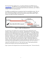
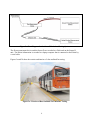
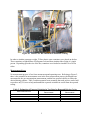
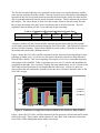
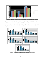
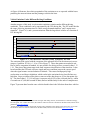
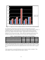
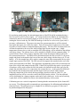
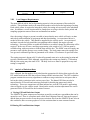
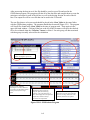
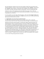
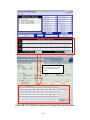
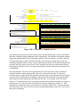
A Study of the Emissions from Diesel Vehicles
Operating in Istanbul, Turkey
January 2007
James Lents, ISSRC
Alper Unal, EMBARQ
Nizamettin Mangir, City of Istanbul
Mauricio Osses, University of Chile
Sebastian Tolvett, University of Chile
Onder Yunusoglu , City of Istanbul
ii
Table of Contents
I. Introduction
II. Testing Procedure
III. Measurement Error
IV. Overall Results
V. Vehicle Emissions Under Different Driving Conditions
VI. Emission Comparisons with the IVE Model
Appendix A: Field Manual for Diesel Vehicle Testing
1
2
5
6
9
12
A.1
List of Tables
Table 1: Diesel Vehicles Tested During the Study
Table 2: Estimation of Expected Variation in Test Data for Repeated Driving Cycles
Table 3: Overall Emission Measurement Results for the Tested Istanbul Diesel Fleet
Table 4: Estimation of Hot Start Emissions for Tested Fleet
Table 5: Potential Adjustment Values to be Used in the IVE Model
Table 6: Recommended Adjustment Values for Use in the IVE model
1
5
7
8
14
15
List of Figures
Figure 1: ISSRC Field Dilution Device
Figure 2: Flow Diagram for the Overall Emissions Testing System
Figure 3a: Exterior of Bus Outfitted for Emissions Testing
Figure 3b: Interior of a Bus Outfitted for Emissions Testing
Figure 4: Emissions Averaged Over Selected Model Years for Heavy Duty Vehicles
Figure 5: Emissions Averaged Over Selected Model Years for Light Duty Vehicles
Figure 6: Comparison of Emissions from Different Vehicle Types
Figure 7a: CO2 Emissions From Heavy Duty Vehicles by IVE Bin
Figure 7b: NOx Emissions From Heavy Duty Vehicles by IVE Bin
Figure 7c: PM Emissions From Heavy Duty Vehicles by IVE Bin
Figure 8a: CO2 Emissions From Light Duty Vehicles by IVE Bin
Figure 8b: NOx Emissions From Light Duty Vehicles by IVE Bin
Figure 8c: PM Emissions From Light Duty Vehicles by IVE Bin
Figure 9: Comparisons of Measured Emission Rates with IVE Predicted Emission Rates
3
4
4
5
8
9
10
10
11
11
12
12
13
14
iii
Introduction
From October 31 to November 17, 2006 a series of 42 diesel vehicles were tested in Istanbul
Turkey. 29 of these vehicles were classified as light-duty vehicles varying from passenger cars
to smaller delivery vans. The tests were carried out in Istanbul at a service garage operated by
the City of Istanbul. Table 1 indicates the vehicles that were tested.
Table 1: Diesel Vehicles Tested During the Study
Engine
Odometer
Size
(km)
(cm3)
Test
Number
Date
Vehicle Type
Model
Year
Weight
(kg)
1
10/31/2006
Light Duty Truck
Hyundai H 100 2.5 TCI
2006
4698
1670
2
10/31/2006
Light Duty Truck
Hyundai H 100 2.5 TCI
2006
23208
1805
3
11/1/2006
Light Duty Truck
Hyundai H 100 2.5 TCI
2006
2476
10314
1805
4
11/1/2006
Light Duty Truck
Hyundai H 100 2.5 TCI
2006
2476
10533
1670
5
11/1/2006
Light Duty Truck
Desoto AS 250
1996
2500
>100000
2300
6
11/2/2006
Light Duty Truck
Tata Telcoline 4x2
2005
1948
60112
1700
7
11/2/2006
Truck
Hino
2001
4009
89358
4400
8
11/2/2006
Minibus
Mercedes Sprinter 412D
1999
2874
>100000
2220
25479
2636+4864
2500
>100000
3500
9
11/2/2006
Truck
Isuzu NPR 66
2005
10
11/3/2006
Light Duty Truck
Ford Transit
1997
11
11/6/2006
Light Duty Truck
Levent L100
2006
>100000
1885
12
11/6/2006
Light Duty Truck
Desoto
1985
>100000
2240+1260
13
11/6/2006
Passenger Car
Renault
2005
1461
50929
945
14
11/6/2006
Passenger Car
Ford Focus Trend
2006
1560
43990
1245
15
11/7/2006
Bus (Public)
Mercedes Citaro
2006
6374
2449
111000
16
11/7/2006
Bus (Public)
MAN SL200
1986
>100000
17
11/7/2006
Bus Articulated (Pub.)
Mercedes 0345
2000
>100000
18
11/8/2006
Bus (Private)
Belde 220CB
2004
>100000
10150
19
11/8/2006
Bus (Private)
Belde Euro 2
2005
>100000
10150
20
11/8/2006
Truck
Desoto AS 250
1996
87 HP
>100000
2300
21
11/9/2006
Truck
Mercedes Axor 3028
2006
6374
10396
12320+6374
22
11/9/2006
Truck
Fiat 50 NC
1987
>100000
2850+2750
23
11/9/2006
Passenger Car
Renault Clio Symbol 1.5
2006
1461
28249
945
24
11/9/2006
Light Duty Truck
Fiat Ducato 230
2001
2800
28263
2040+984
25
11/10/2006
Truck
Isuzu NQR 70P
2006
5193
626
5460+2041
26
11/10/2006
Light Duty Truck
Isuzu NKR Wide 66
2001
4334
65119
3050
27
11/10/2006
Minibus
Mercedes Sprinter 308D
1997
79 HP
>100000
2005
28
11/13/2006
Truck
Mercedes Benz
1997
211 HP
>100000
10520+14930
29
11/13/2006
Light Duty Truck
Fiat Doblo Combi 1.9
2004
1910
15442
1350+735
30
11/13/2006
Light Duty Truck
Fiat Doblo Combi 1.9
2004
1910
10668
1350+735
31
11/13/2006
Minibus
Ford Transit 300S
2006
2402
22207
2010
32
11/14/2006
Minibus
Ford Otosan
2006
2402
25042
2010
33
11/14/2006
Minibus
Volkswagen Transporter
1997
78 HP
>100000
1705+995
34
11/14/2006
Minibus (Commercial)
Otokar
2006
3770
26982
3660
35
11/14/2006
Truck
Fatih
1987
6550
36
11/15/2006
Light Duty Truck
Ducato 230
2001
2800
>100000
>100000
1910
>100000
1380
37
11/15/2006
Light Duty Truck
Fiat Doblo Cargo 1.9
1
2003
2040
38
11/15/2006
Light Duty Truck
Mercedes Benz 312D
1998
2874
>100000
1045+2455
39
11/15/2006
Minibus
Ford Transit 100
2000
2490
41502
1530+1180
40
11/15/2006
Passenger Car
Renault Clio Symbol 1.5
2006
1461
17813
945
41
11/16/2006
Light Duty Truck
Dodge Chrysler
1996
2500
>100000
3500
42
11/16/2006
Light Duty Truck
Levent L100
2006
2593
7952
1885+1265
This study was a joint effort of the City of Istanbul, EMBARQ, and ISSRC. The City of Istanbul
provided a location for testing, personnel to install testing equipment and procured vehicles for
testing. EMBARQ also supplied personnel to support testing and participated in the selection of
vehicles for testing. ISSRC provided test equipment and testing expertise for the study.
Testing Procedure
Vehicles were brought to the test site for test equipment installation. These vehicles were
warmed up at the time of the testing. Once emissions testing equipment was installed, the
vehicles were operated over a prescribed driving circuit that Istanbul allowed the vehicles to be
operated over as wide a range of operating conditions as could be achieved within the city limits
of Istanbul. The driving circuit required from 36 to 50 minutes to complete depending upon the
traffic situation and included a moderate hill that the vehicles drove over. The typical time to
complete the circuit was 38 minutes.
For emission measurement purposes, a Semtech Sensor D gas emissions testing unit was used to
measure the emissions of CO, CO2, total Hydrocarbons (THC), NOx, and NO2. The Sensor D
unit uses infrared absorption technology to measure CO and CO2 , ultraviolet absorption
technology to measure NOx and NO2, and a flame ionization detector to measure total
hydrocarbon emissions. The Sensor D testing unit is an integrated emissions testing device
designed to be used in on-road testing programs. The Sensor D measures emission
concentrations and must be provided with exhaust flow rates and ambient temperatures and
pressures in order to determine mass emission rates. The Sensor D is equipped with a
temperature/pressure sensor. A Semtech manufactured 4 inch (10 cm) exhaust flow
measurement device was used to measure the exhaust flow rate from the bus. This device uses
standard dynamic and static pressure measurement to calculate exhaust flow. The Sensor D was
also equipped with a GPS device to measure location and speed. All data was collected at one
second intervals. For further information on the Sensor D test unit and the Semtech exhaust flow
device please go to www.sensors-inc.com . The Sensor D test unit was zeroed and spanned at
each set of test cycles. The unit was found to be very stable from day to day with the zero and
span holding within 1% of the calibration gases.
Particulates were measured on a second by second basis using a Dekati DMM testing unit. This
unit uses a particle charging process and six stage impactor setup to determine particle mass.
The DMM measures particle concentration. The exhaust flow rates collected by the Sensor D
unit must be used with the Dekati measurements to determine particulate mass flow rates. The
DMM measures particles in the 0 to 1.5 micron range, which is the size range where virtually all
diesel particulates reside. The DMM has been found to produce results comparable to the
reference particulate sampling methods for diesel particulates; although, it was found to produce
readings about 30% high in some cases. Dekati experts believe that this is due to the fact that the
Dekati measurement process can measure volatile particulate matter that is lost in the case of
2
filter based particulate sampling devices. For further information on the DMM, please see
www.dekati.com. The DMM was zeroed at the beginning of each testing cycle. The charging
and impactor units become covered with particulates and must be cleaned after each 2-3 hours of
testing to keep the unit operating properly.
The DMM can not handle the mass concentrations found in uncontrolled diesel units. Thus, the
diesel exhaust must be diluted at a controlled rate in order to use the DMM. A field dilution
device was developed by ISSRC to use in on-road emissions testing with the DMM. Figure 1
illustrates the design of the ISSRC field dilution unit.
Figure 1: ISSRC Field Dilution Device
The exhaust flow in the dilution device is measured using a Dwyer differential pressure
transducer, which is accurate to 0.25% of full scale. The differential pressure gauge is used to
measure the pressure difference between P2 and P3 shown in Figure 1. A micro-filter produces
particle free air to be diluted with the exhaust sample. The exhaust sample and dilution air are
heated to 110 degrees C to avoid water and organic condensation. The dilution control can be
adjusted to levels from 20 to 1 to 40 to 1 using the ball valve dilution control at the inlet to the
micro-filter. Unfortunately, when the exhaust gases flowing through the exhaust flow device
increase as the vehicle accelerates, the pressure P1 in Figure 1 drops and the dilution rate
changes. Thus, the dilution rate must be monitored second by second and the dilution rates
corrected second by second to produce an accurate particulate mass emissions rate. On occasion
when testing a large engine under heavy load, the pressure P1 drops so low as to reduce the
exhaust flow in the diluter to near zero. This causes the system to under predict particulate
emission rates and must be removed in the data analysis process.
Figure 2 presents a flow diagram for the overall emissions testing system. The data collected by
3
Figure 2: Flow Diagram for the Overall Emissions Testing System
The flow measurement device and the Sensor D are recorded to a flash card on the Sensor D
unit. The Dekati information is recorded to a laptop computer that is connected to the Dekati by
a serial cable.
Figures 3a and 3b show the exterior and interior of a bus outfitted for testing.
Figure 3a: Exterior of Bus Outfitted for Emissions Testing
4
Figure 3b: Interior of a Bus Outfitted for Emissions Testing
In order to simulate passenger weight, 70 liter plastic water containers were placed on the bus.
These containers weighed about 64 kilograms each and thus simulated the weight of a single
person. Depending upon the size of the bus, containers were loaded to simulate 30 to 50 bus
riders.
Measurement Error
No measurement process is free from measurement and operating error. Referring to Figure 2,
there is the potential for measurement error in the flow measurement process, the dilution rate
measurement, the gas concentrations measurement, and the bus operator's ability to follow the
desired driving patterns. Table 2 outlines potential error assuming that each process can be held
to produce only 2% error to help understand the expected variations in results from the repeated
testing.
Table 2: Estimation of Expected Variation in Test Data for Repeated Driving Cycles
Impact on Gaseous
Measurements
2%
--2%
4%
Measurement Process
Exhaust Volume Flow Measurement
Dilution Measurement
Emissions Concentration Measurement
Total Potential Variation
5
Impact on Particle
Measurements
2%
2%
2%
6%
To further complicate the process, data is collected on normal city streets which results in
different driving patterns from test to test. Daily variations in traffic flow have a major impact
on how the vehicles can be operated. Thus, emissions can vary considerably from test to even
using the same vehicle. To correct for this variation, the data is divided into different power
demand categories. 60 power demand categories are used for this purpose. These categories are
typically referred to as Power Bins and are numbered from 0 to 59. The distribution of driving in
the 60 Power Bins is determined. This driving distribution is multiplied by the average
emissions measured in the 60 bins to produce a standardized estimate of emissions that would
have resulted if the vehicle had been operated on an FTP cycle. This approach was found in a
yet to be published study in Brazil to produce estimates of emissions on the actual driving cycle
within 6%. While this is good in many respects, it must be added to measurement uncertainty
indicated in Table 2, which results in a potential emissions error of 10-12% overall. The error
discussed in the previous paragraphs should be random and thus should average out to some
degree over multiple tests.
Finally, the number of vehicles that can be tested in a 2-3 week period is limited. This limited
testing further decreases the certainty of how will the tested fleet actually represents the actual
urban fleet. Based on ISSRC data collected in similar gasoline emissions studies, the collection
of data from a fleet of randomly selected gasoline fueled vehicles resulted in 90% confidence
interval of plus or minus 20%.
When all potential errors are combined, it should be anticipated that this study will produce
results which are to a 90% probability to within 25-30% of the actual emissions produced by the
local fleet. While this potential error is larger than preferred, it is still better than using emission
estimates derived from studies in the U.S. and Europe. In the long run, more emissions tests are
required in order to reduce the mobile source inventory uncertainty to the 10% range.
Overall Results
Table 3 presents the average emissions measured for the various vehicles tested in the program.
They are listed in the order tested. An average value and 90% confidence limits are also
included. The 90% confidence interval in Table 3 indicates the range of emissions for which
there is a 90% probability that the true mean emission rate of the fleet would exist if the tested
vehicles were randomly selected from the Istanbul fleet. The vehicles tested should be
somewhat representative of the Istanbul fleet, thus, the measured values are likely within 20-25%
of the true mean of the Istanbul fleet.
6
Table 3: Overall Emission Measurement Results for the Tested Istanbul Diesel Fleet
Test
Date Tested
Number
Vehicle Type
Measured Emissions
(grams/kilometer)
Year
FTP Normalized Emissions (grams/kilometer
CO2
NOx
PM
CO
THC
CO2
NOx
PM
CO
THC
1
10/31/2006
Light Duty Truck
2006
290
1.26
0.011
0.00
0.18
214
1.09
0.008
0.00
0.11
2
10/31/2006
Light Duty Truck
2006
361
1.48
0.066
0.00
0.39
259
1.19
0.046
0.00
0.25
3
11/1/2006
Light Duty Truck
2006
343
1.02
0.045
0.71
0.16
264
0.95
0.035
0.56
0.11
4
11/1/2006
Light Duty Truck
2006
292
0.000
0.94
0.25
270
0.82
0.000
0.81
0.22
5
11/1/2006
Light Duty Truck
1996
602
0.96
13.5
0.134
2.55
1.83
385
10.14
0.085
1.63
1.02
6
11/2/2006
Light Duty Truck
2005
292
1.24
0.055
0.21
0.07
235
1.06
0.043
0.16
0.06
7
11/2/2006
Truck
2001
451
2.99
0.105
3.04
1.57
363
3.13
0.087
2.51
1.11
8
11/2/2006
Minibus
1999
303
1.22
0.142
1.37
0.38
242
1.24
0.114
1.09
0.26
9
11/2/2006
Truck
2005
559
4.43
0.146
2.92
1.37
372
3.80
0.100
1.98
0.76
10
11/3/2006
Light Duty Truck
1997
367
4.14
0.084
0.91
0.70
243
3.27
0.054
0.61
0.38
11
11/6/2006
Light Duty Truck
2006
349
3.20
0.032
2.16
1.58
293
2.73
0.027
1.78
1.25
12
11/6/2006
Light Duty Truck
1985
96
2.14
0.151
0.71
0.52
65
1.89
0.103
0.49
0.30
13
11/6/2006
Passenger Car
2005
203
1.73
0.073
1.58
0.23
132
1.39
0.047
0.99
0.12
14
11/6/2006
Passenger Car
2006
234
1.23
0.188
0.28
0.02
168
0.88
0.114
0.17
0.01
15
11/7/2006
Bus (Public)
6.75
0.67
857
10.09
0.076
4.85
0.41
16
11/7/2006
4.26
2.46
674
13.33
0.299
3.13
1.47
17
11/7/2006
2006 1198 11.41 0.105
Bus (Public)
1986 949 14.33 0.413
Bus Articulated (Pub.) 2000 1574 20.88 0.025
1.60
1.06
1212
19.66
0.020
1.24
0.71
18
11/8/2006
Bus (Private)
2.33
1.34
669
11.66
0.413
1.45
0.66
19
11/8/2006
Bus (Private)
3.71
0.44
579
7.11
0.446
3.12
0.32
20
11/8/2006
Truck
2004 1089 13.43 0.665
2005 701 7.09 0.533
1996 484 14.11 0.112
3.14
1.46
385
15.05
0.091
2.55
0.99
21
11/9/2006
Truck
2006
748
10.06 0.163
2.06
0.27
540
10.16
0.121
1.55
0.16
22
11/9/2006
Truck
1987
448
9.32
0.176
6.70
3.25
253
7.18
0.099
3.83
1.47
23
11/9/2006
Passenger Car
2006
205
1.84
0.000
0.84
0.06
141
1.39
0.000
0.55
0.04
24
11/9/2006
Light Duty Truck
2001
449
4.87
0.147
2.37
0.52
216
3.23
0.071
1.17
0.20
25
11/10/2006
Truck
2006
653
4.54
0.076
2.77
0.51
489
3.98
0.057
2.06
0.33
26
11/10/2006
Light Duty Truck
2001
406
3.65
0.125
2.43
1.56
365
3.99
0.115
2.25
1.25
27
11/10/2006
Minibus
1997
382
1.85
0.141
0.86
0.16
193
1.42
0.072
0.44
0.06
28
11/13/2006
Truck
1997
858
12.03 0.113
4.49
2.27
447
9.97
0.061
2.39
0.91
29
11/13/2006
Light Duty Truck
2004
186
0.98
0.043
0.20
0.11
216
0.98
0.046
0.21
0.13
30
11/13/2006
Light Duty Truck
2004
308
1.41
0.089
0.66
0.13
196
1.05
0.055
0.41
0.07
31
11/13/2006
Minibus
2006
272
1.32
0.132
3.35
0.87
132
0.94
0.065
1.64
0.33
32
11/14/2006
Minibus
2006
241
1.57
0.134
0.65
0.29
152
1.11
0.082
0.40
0.16
33
11/14/2006
Minibus
1997
163
1.32
0.073
0.74
0.11
91
0.82
0.035
0.35
0.05
34
11/14/2006
Minibus (Commercial) 2006
469
5.62
0.126
2.31
0.65
377
5.05
0.104
1.91
0.49
35
11/14/2006
Truck
794
15.61 0.448 10.12
2.97
447
12.68
0.257
5.82
1.35
36
11/15/2006
Light Duty Truck
3.95
90
2.58
0.007
0.85
0.19
37
11/15/2006
Light Duty Truck
0.14
137
1.31
0.021
0.29
0.05
38
11/15/2006
Light Duty Truck
0.49
213
2.08
0.068
1.50
0.28
39
11/15/2006
Minibus
2001 1151 11.60 0.094 10.78
2003 276 1.80 0.042 0.61
1998 312 2.36 0.098 2.17
2000 269 3.02 0.037 1.38
0.36
177
2.45
0.024
0.90
0.20
40
11/15/2006
Passenger Car
2006
82
0.76
0.012
1.19
0.11
45
0.53
0.006
0.65
0.05
41
11/16/2006
Light Duty Truck
1996
456
13.08 0.044
3.00
1.79
215
15.67
0.021
1.43
0.54
42
11/16/2006
Light Duty Truck
2006
389
CO2
3.43
NOx
2.42
CO
1.56
THC
240
CO2
2.47
NOx
0.054
PM
1.41
CO
0.83
THC
1987
0.093
PM
Average Values
482
8.54
0.13
2.41
0.92
316
7.36
0.09
1.45
0.47
90% Confidence Interval
17%
16%
27%
25%
26%
18%
17%
28%
22%
24%
7
The first 200 seconds of driving were separated out since there was concern that there could be
some start-up emissions from the vehicles. Start-up emissions were estimated by calculating the
emissions in the first 200 seconds based on emissions measured in the vehicle test after the first
200 seconds and subtracted from the actual measured emissions. Table 4 indicates the results of
this analysis. The values shown in Table 4 are the average values for the total tested fleet and
have a large uncertainty since they involve a difference and a correction process. The 90%
confidence interval shown in Table 4 is an indicator of this uncertainty.
Table 4: Estimation of Hot Start Emissions for Tested Fleet
Average Excess Emissions
CO2
(grams/start)
-19.0
NOx
(grams/start)
-0.63
PM
(grams/start)
0.04
CO
(grams/start)
0.45
THC
(grams/start)
-0.03
90% Confidence Interval
103%
53%
85%
77%
280%
A negative number in Table 4 means that the emissions measured after the first 200 seconds
were actually greater than the emissions during the first 200 seconds. Only PM and CO showed
positive hot start emissions. Little reliance should be placed on these values due to the large
uncertainty indicated by the confidence interval.
Figure 4 shows the CO2, NOx, and PM emissions from the larger trucks and emissions for three
groupings of model years. As can be seen, the data for the newer vehicles are little difference
from the older vehicles. This is not surprising with respect to CO2, but is somewhat surprising
with respect to NOx and PM. Table 4 represents tests over only 13 vehicles and should thus be
considered in that light. Also, two buses, both by the same manufacturer, out of 6 vehicles in the
2004-2006 measured emissions 4 times higher than the other buses. If these two buses are
removed from the data set then the emission rate for the newer vehicles is about the same as the
1996-2001 average.
25.0
20.0
15.0
1986
-1987
1996
-2001
10.0
2004
-2006
5.0
0.0
CO2/40
Nox
PM*100
Figure 4: Emissions Averaged Over Selected Model Years for Heavy Duty Vehicles
Figure 5 shows the CO2, NOx, and PM emissions from the passenger vehicles and smaller trucks
tested in the study. These results, which represent 29 tests, show some reduction in emissions
from 1986 to 2006; although the improvement is not major.
8
9
8
7
6
1985
-1999
5
2000
-2004
4
3
2005
-2006
2
1
0
CO2/40
Nox
PM*50
Figure 5: Emissions Averaged Over Selected Model Years for Light Duty Vehicles
The particulate emissions from these vehicles are significant. They are in the ballpark of
particulate emissions from the larger diesel vehicles.
It is also valuable to consider emissions by vehicle type. These values are shown in Figure 6 for
five pollutants of interest.
7
1600
6
1400
5
1200
1000
4
800
3
600
2
400
1
200
0
0
Bus
Truck
Pickup Truck MiniBus
Passenger
Vehicle
18
Bus
Truck
Pickup Truck MiniBus
Passenger
Vehicle
Pickup Truck MiniBus
Passenger
Vehicle
0.6
16
0.5
14
12
0.4
10
0.3
8
6
0.2
4
0.1
2
0
0
Bus
Truck
Pickup Truck MiniBus
Passenger
Vehicle
Bus
Truck
Pickup Truck MiniBus
Passenger
Vehicle
2.5
2
1.5
1
0.5
0
Bus
Truck
Figure 6: Comparison of Emissions from Different Vehicle Types
9
As Figure 6 illustrates, the relative magnitude of the emissions were as expected with the buses
producing the most emissions and the passenger vehicles the least.
Vehicle Emissions Under Different Driving Conditions
Another purpose of this study is to determine emissions variation under different driving
conditions. These conditions can be represented by the IVE driving bin. The IVE model divides
the range of driving situations into 20 vehicle energy demand situations1 and 3 engine stress
situations2. Figure 7a, b, and c present emissions from the large diesel vehicles as a function of
IVE driving bin.
35
30
25
20
15
10
5
0
1.00
1.04
1.08
1.12
1.16
2.00
2.04
2.08
2.12
2.16
3.00
3.04
3.08
3.12
3.16
Figure 7a: CO2 Emissions From Heavy Duty Vehicles by IVE Bin
The emissions look typical with the exception of the apparent fall off in emission rate in stress
category 1 and bins 16-18 (i.e. 1.16 to 1.18 in Figure 7). These data points are marked in red.
Due to traffic congestion in Istanbul, it is not possible for driving to have occurred in bins 1.171.19. Thus, these data points must result from erroneous classification of data into bins. It has
been found that the GPS unit will loose signal and freeze and then jump to the correct speed
when the signal returns or miscalculation of altitude. This causes an improperly high
acceleration or road slope calculation, which results in the emissions being classified into too
high bins. Steps are taken to filter these events out of the data; however, a few data points slip
by. The data in bins 1.17-1.19 in Figure 6 represent only 0.02% of the collected data (i.e. about
6 seconds out of 2,600,000 seconds of data) and are included only for the sake of completeness.
Figure 7b presents data from the same vehicles but this data is the NOx data from those vehicles.
1
The energy demand on a vehicle is the result of engine and rolling friction, wind resistance, acceleration energy,
and road grade. For a further discussion, the reader is referred to the user’s manual for the IVE model, which can be
obtained at www.issrc.org/ive .
2
Engine stress relates to engine rpm and the average energy demand on the vehicle in the most recent 15 seconds.
The reader is referred to the user’s manual for the IVE model, which can be obtained at www.issrc.org/ive .
10
0.3
0.25
0.2
0.15
0.1
0.05
0
1.00
1.04
1.08
1.12
1.16
2.00
2.04
2.08
2.12
2.16
3.00
3.04
3.08
3.12
3.16
Figure 7b: Emissions From Heavy Duty Vehicles by IVE Bin
There is one interesting aspect of this data set. There is data in bins 1.14 and 1.15 that have
dropped off even with significant driving in those bins. Thus, the fall off in NOx emissions in
bins 1.14 and 1.15 may be a real phenomenon. This characteristic is seen in gasoline data were
the vehicles go into an enrichment mode that reduces the combustion temperatures and thus
NOx. These vehicles may be doing the same thing.
Figure 7c presents the binned data for particulate matter from the large diesel vehicles. This data
is more discontinuous than the NOx or CO2 data. A part of this discontinuity may be the extra
error induced by the requirement to use a diluter and the change in the performance of the Dekati
particulate test unit as it becomes dirty. In any case, the general form of the emissions curve can
still be seen in the data.
0.006
0.005
0.004
0.003
0.002
0.001
0
1.00
1.04
1.08
1.12
1.16
2.00
2.04
2.08
2.12
2.16
3.00
3.04
3.08
3.12
3.16
Figure 7c: PM Emissions From Heavy Duty Vehicles by IVE Bin
Figure 8a, b, and c present the same data as Figures 7a, b, c except that it comes from the light
duty diesels tested in Istanbul. The data points marked in red again represent erroneous data
points since no driving could have occurred in these bins. Otherwise, the data looks reasonable
for these types of vehicles.
11
9
8
7
6
5
4
3
2
1
0
1.00
1.04
1.08
1.12
1.16
2.00
2.04
2.08
2.12
2.16
3.00
3.04
3.08
3.12
3.16
Figure 8a: CO2 Emissions From Light Duty Vehicles by IVE Bin
0.06
0.05
0.04
0.03
0.02
0.01
0
1.00
1.04
1.08
1.12
1.16
2.00
2.04
2.08
2.12
2.16
3.00
3.04
3.08
3.12
3.16
Figure 8b: NOx Emissions From Light Duty Vehicles by IVE Bin
It is difficult to know if there is a similar enrichment in the NOx resulting in emissions
reductions in the higher bins in this data set.
Figure 8c presents the binned PM emissions. As was the case with the larger diesel vehicles, the
binned emissions are more discontinuous compared to the CO2 and NOx emissions.
12
0.0035
0.003
0.0025
0.002
0.0015
0.001
0.0005
0
1.00
1.04
1.08
1.12
1.16
2.00
2.04
2.08
2.12
2.16
3.00
3.04
3.08
3.12
3.16
Figure 8c: PM Emissions From Light Duty Vehicles by IVE Bin
The particulate emissions follow the expected pattern on the whole.
Emission Comparisons with the IVE Model
As noted earlier, 13 large buses and trucks and 29 smaller passenger cars and trucks were tested
in Istanbul. This limited data does not provide large enough samples of individual technologies
to do an analysis of emission comparisons by technology type. Instead, the IVE model was run
using an FTP driving pattern, the pattern used to develop base emission factors for the IVE
model, using the distribution of vehicles tested in Istanbul. Two vehicle groups were used. The
first was the 13 larger diesel vehicles and the second was the 29 smaller diesel vehicles. The
average measured values normalized to FTP driving cycles were divided by the IVE predicted
values to evaluate the comparisons. Figure 9 provides the results of this analysis.
As can be seen, the CO2 emission projections were accurate producing a ratio close to 13. The
other predictions, however, showed a wide variance. The PM values measured were less than
those predicted by the IVE model. Differences between actual and measured values were
anticipated in the development of the IVE model and provisions are made in the IVE model to
add an adjustment file that will adjust the base emission factors to actual measured values.
3
In the case of light duty vehicles the ratio is 0.94. In the case of the heavy duty vehicles the ratio is 0.97. These 36% differences are well within the accuracy of the data collection process.
13
2.50
2.00
1.50
Overall Truck
Overall Auto
1.00
0.50
0.00
CO Ratio
VOC Ratio
NOx Ratio
PM Ratio
CO2 Ratio
Figure 9: Comparison of Measured Emission Rates with IVE Predicted Emission Rates
The default base emission factors in the IVE model are based primarily on emission
measurements made in the United States and represent test results from thousands of vehicles. It
is difficult to know how much weight to give to emission results from only 42 vehicles.
However, the confidence limits shown in Table 3 suggest that the results should be in the
ballpark of 30% of the measured values. Table 5 shows the actual ratios and the ratios if the
measured emission results were modified to be 30% closer to the IVE projected values.
Table 5: Potential Adjustment Values To Be Used in IVE Model
Class
Overall Truck (Heavy Duty Vehicles)
Overall Truck Adjusted 30% in direction of default values
Overall Auto (Light Duty Vehicles)
Overall Auto Adjusted 30% in the direction of default values
CO Ratio
0.46
0.60
VOC Ratio
0.70
0.91
NOx Ratio
0.74
0.96
PM Ratio
0.45
0.60
0.72
0.93
0.95
1.23
2.18
1.53
0.70
0.91
Because of the limited number of tests, it is suggested that the values closer to the IVE default
values (the 30% adjusted values) be used until more in-use emissions data is collected. A value
of 1 is used in the cases where the 30% adjustment takes the values from less than 1 to greater
than 1.
Table 6 presents the recommended adjustment values for diesel vehicles in Istanbul. These
values should, of course, be improved as more data is collected.
14
Table 6: Recommended Adjustment Values for Use in the IVE model
Class
CO Ratio
0.60
0.93
Overall Diesel Heavy Duty Vehicle
Overall Diesel Light Duty Vehicle
15
VOC Ratio
0.91
1.00
NOx Ratio
0.96
1.53
PM Ratio
0.60
0.90
Appendix A
Field Manual For Diesel Vehicle Testing
A.1
IVE In-Use Vehicle Emissions Study for Diesel Vehicles
I. Introduction:
Diesel emissions are important contributors to air quality degradation in urban areas. Diesel
particulates are considered to be carcinogenic or likely carcinogens in the United States, and
diesels are often the prime source of nitrogen oxide emissions. It is thus important that diesel
emissions be well understood and that air quality planners be able to predict the impact of diesels
in the present time and at times in the future based on specific control scenarios. To support
these efforts, a process of on-road measurement of diesel emissions has been devised and the
International Vehicle Emissions (IVE) model was developed to estimate emissions from diesel
vehicles under different driving and control scenarios.
The IVE model is designed to make estimates of in-use vehicle emissions in the full range of
global urban areas. At the point in time of IVE model development, data to establish base
emission factors and driving pattern adjustments were, of necessity, based on vehicle studies
carried out primarily in the United States. This has raised questions as to the applicability of the
base emission rates and driving pattern adjustments used in the model to developing countries.
The IVE in-use vehicle emissions study is designed to test the hypothesis that similar vehicle
technologies will produce equivalent emission results in a given location and to provide some
rudimentary data for creating improved emission factors.
The IVE modeling framework provides the user with the ability to enter adjustments to the base
emission factors that are specific to a location in case the supplied factors are found to be in
error. This capability was built into the model to support emission measurement studies that
would be made in developing countries as local capacity increases. The IVE In-Use vehicle
emissions study is not designed to fully develop correction factors for the IVE model. The
original data base used to developed the IVE model correction factors was based on more than
500 vehicle tests each involving three driving cycles carried out at the University of California
CE-CERT research facility. This information was combined with summarizations of thousands
of in-use vehicle tests provided by the United States Environmental Protection Agency. The IVE
In-Use emissions study discussed in the following section results in emissions data for 40 diesel
fueled vehicles. Information from 40 vehicles, while significant, does not provide the range of
data for the development of a full range of new emission factors and adjustments. Nonetheless,
the IVE In-Use emissions study can be used to make rudimentary adjustments to the IVE model
that will certainly improve its performance for developing countries.
The actual IVE In-Use vehicle emissions study makes use of recently developed emissions
measurement technology that can be carried on-board vehicles while they are driven on urban
streets. This technology allows emission mass per unit distance to be determined in real driving
situations. To date, this on-board emissions measurement technology can be used to measure
carbon monoxide (CO), carbon dioxide (CO2), total hydrocarbons (THC), and nitrogen oxides
(NOx). A different testing device to measure particulate emissions is also used during the study
to establish real-time particulate emissions from the tested diesel vehicles.
A.2
The IVE in-use vehicle emissions study is built around a two week study period where on-road
vehicle emissions data is collected.
II.
Equipment Needed to Complete Study
A wide range of equipment is required to carry out the diesel emissions study. The key pieces of
equipment will be shipped from the United States. However, a significant amount of equipment
and supplies must be provided locally. An Excel spreadsheet program is provided with this
write-up that indicates the equipment that will be sent from the United States and the equipment
that must be procured locally.
III.
Sample Size and Impact on Emissions Measurement Reliability:
Unfortunately for the researcher studying the emissions from on-road vehicles, the variance in
emissions among vehicles with similar technologies is quite large. This means that multiple tests
on different vehicles are required to accurately establish the true fleet wide average for a given
technology. Equation II.1 indicates the 70% confidence interval for data in a Gaussian
distribution.
I70% = ± σ/√ (n-1)
where,
I70% = 70% confidence interval
σ = standard deviation
n = sample size
II.1
In the case of vehicular emissions, σ is often close to the sample mean; although diesel vehicles
show a little less variation that do gasoline fueled vehicles. In this case, Equation II.1 becomes:
I70% = ±[M/√(n-1)]
where M = measured sample mean
II.2
In this special case, to insure that the measured mean has a 70% probability of being within 15%
of the actual mean requires a sample size of 44 vehicles. The actual variation in emissions from
similar technologies is unknown but based on the previous discussion it is clear that a relatively
large number of vehicles of a given technology class should be tested. For purposes of this
study, at least 10 vehicles of each important technology should be measured to insure even a
moderate level of confidence in the results. Once the data is collected, the variance in the data of
similar vehicles will establish the true confidence that can be placed in the results of the tests.
With present vehicle testing technology, about 1.5 hours are required to remove the equipment
from one vehicle and install the sampling equipment in a second vehicle. To collect data for ¾
of an hour for a given vehicle will thus require a total of 2.25 hours per vehicle. In a 9 hour day,
about 4 vehicles can be sampled. In a two week sampling period (10 sampling days), about 40
vehicles can be studied. Thus, based on the preceding discussion, only four general vehicle
technology groups should be studied over the two week sampling period in order to insure at
A.3
least 10 vehicles per technology class are studied. The variety of diesel engine technologies
operating in most urban areas today are relatively small and the study of the four most
predominate vehicle technologies in an area will provide useful data for understanding the
overall diesel emissions in an urban area.
IV.
Sampling Program:
Based on Section II, it is desired to study four vehicle technology classes during the two week
study. The vehicle technology classes that should be studied are those groups which dominate
the local diesel fleet being studied and which will continue to be important in the next 5 years.
The vehicles selected may vary from location to location, but based on previous experience, it is
suggested that the following four technology classes be considered:
1.
2.
3.
4.
Euro 1 type technologies
Euro 2 type technologies
Euro 3 type technologies
Euro 4 type technologies if available or extend testing of most common of the
three previous groups.
The previous suggested technology classes should not be rigidly adhered to in cases where the
local fleet does not contain significant numbers of vehicles in any of the vehicle classes listed. It
is best to tailor the study to the makeup of the local fleet. For this paper, the four suggested
classes will be used for discussion purposes.
Start emissions are important for gasoline vehicles but are not considered as important for diesel
vehicles. Thus the testing program that will be used will not collect diesel vehicle start
emissions. Vehicles will be scheduled to be brought to the testing area at 2.25 hour intervals
beginning at 08:00. Thus a second vehicle will be due at 10:15. (On the first day only two tests
should be scheduled to allow for proper on-site training.) It is critical that vehicles not arrive
late. It is best to schedule them to arrive a little early. The new vehicles will be parked in the
test area leaving room for the returning vehicle to be parked. Once the vehicle being tested
arrives at the test setup facility, the equipment is moved from the tested vehicle and installed in
the new vehicle that has arrived for testing. Buses are expected to arrive with only a driver.
Sand bags will be loaded onto the bus to simulate passenger weight. Trucks should arrive with a
half to a full load for purposes of testing. The truck or bus will be at the facility for about 3
hours for equipment installation, testing, and equipment removal. It can then be returned to its
owner.
A.4
Figure 1: Truck and Bus with Flow Measurement Devices Connected to the Exhaust
V.
Vehicle Driving Procedure:
Table IV.1 indicates the approach that will be used to test the vehicle. The driving roads selected
for the study should provide for convenient stopping locations that will occur at the desired time
intervals and return the vehicle to the starting point at the desired time. The roads selected
should also allow for as great a variety of driving as feasible for the location.
It is critical that vehicles arrive on time. A testing facilitator should be in touch with the vehicle
suppliers to insure that the vehicles will arrive on schedule.
Table IV.1: Vehicle Driving Procedure
Step
1
2
3
4
5
6
7
8
9
Procedure
A vehicle arrives at the test setup facility at the designated appointment
time while previous vehicle is being tested.
Vehicle will be parked in the next vehicle test setup location
Vehicle will be studied and a decision will be made as to the best way to
attach testing equipment to the just arrived vehicle. Sand bags are loaded
onto vehicle to be tested.
Tested vehicle returns to the test setup location and parks near the next
vehicle setup location.
Download data from the just tested vehicle
Test equipment is removed from tested vehicle and transferred to new
vehicle and tested vehicle released for return to the owner.
Equipment installed on new vehicle.
Data collection initiated and vehicle started and driven over the
designated one-hour test route.
Total time to test one vehicle
Time Interval
---5 minutes
20 minutes
5 minutes
5 minutes
30 minutes
25 minutes
45 minutes
135 minutes
Traffic will of course impact the distances that will be covered during the driving phase. Thus,
the test route should be designed so that there are alternate routes to be taken so that the vehicle
can complete its test run in the 45 minutes that are allocated. Since traffic will flow better at
various times of the day, the test may be completed in 30 minutes in one case and in 60 minutes
in another case. The test route should be selected so that the vehicle can complete the test run in
60 minutes in the worst traffic. It is also critical that the driving course selected contain street
sections where higher speeds and accelerations can be achieved as well as slower speeds and
lower accelerations. The driver should operate the vehicle in a manner typical of the traffic that
A.5
is occurring at the time of testing and in the manner that the vehicle is normally used (i.e., a bus
will stop at bus stops even though it does not pick up or discharge passengers). Buses and trucks
should be marked with signs taped to the vehicle indicating that the vehicle is participating in a
testing program.
VI.
Vehicle Procurement:
Procuring 40 large diesel vehicles for testing with a driver and, in the case of trucks, can be a
challenge. Bus companies must be contacted as well as trucking companies to find the desired
vehicles.
In both Mexico City and Sao Paulo, a $US50 per vehicle fee was paid for gasoline fueled
vehicle. This fee plus the use of contacts at the partnering agencies provided all of the needed
vehicles in Sao Paulo. In the case of buses and trucks a higher fee may be necessary unless
representative buses can be obtained from government sources supportive of the testing program.
It is recommended that $200-$300 be set aside for payment to bus/truck owners for providing a
vehicle and driver for the approximate 3 hour testing program. However, this is a local decision
that should be made.
VII.
Vehicle Sampling Equipment:
For purposes of these studies a SEMTECH-D portable emissions monitor (PEM), manufactured
by Sensors, Inc., will be used for gaseous emissions. This unit employs a flame ionization
detector (FID) to measure THC, a Non-Dispersive Ultraviolet (NDUV) analyzer to measure NO
and NO2, a Non-Dispersive Infrared (NDIR) analyzer to measure CO and CO2, and an
Electrochemical sensor to measure O2. Fuel for the FID is provided via a high-pressure canister
mounted within the PEM. For measuring particulate emissions, a Finnish Dekati testing unit will
be used to collect second by second particulate emissions data. The Dekati test unit makes use of
technology that ionizes the particulates and collects them by size. A whole-exhaust, mass flow
measurement device will measure the exhaust flow rate based on static and dynamic pressure
differentials. A partial stream of the exhaust, taken from within the mass flow measurement
device, is routed through the analyzer system at a constant rate of 10 liters per minute. The
concentration and flow rate data is input to the onboard data logger on a second by second basis.
Internal filters, carbon absorbers, and chillers are strategically located in the sample stream to
minimize interferences. A temperature and humidity measurement device also provides second
by second data on the temperature and humidity of the engine intake air. Algorithm’s in the
processing software provide the necessary adjustment to the NO and NO2 results from the
NDUV based upon the humidity of the intake air. Data, also collected on a 1 hertz cycle, from
an onboard GPS unit allows the measured mass of each pollutant to be matched up with the
driving activities of the vehicle.
The PEM, including protruding knobs and connectors, measures 404 mm in height by 516 mm in
width by 622 mm in depth. It weighs approximately 35 kg. The ID of the mass flow
measurement device will have a diameter of 10.2cm.
A.6
Figure 2: A Bus and Truck with Equipment and Sandbags Loaded
Except during actual testing, the internal temperatures of the PEM will be maintained using a
line-serviced 12-volt DC power supply. A Y-connector allows the PEM to be simultaneously
connected to the line-serviced power supply as well as a deep-cycle 12-volt battery. Prior to
starting the first test each day, the PEM will undergo a leak test as well as a zero, span, and, if
necessary, calibration test. The proper size mass flow measurement device will be selected
based upon the engine size of the test vehicle. This will insure that a backpressure of less than
ten inches of water column is maintained during the testing. The mass flow measurement device
will then be attached to the rear of the vehicle using high vacuum suction cups. A hightemperature silicone sleeve, sized to match the OD of the tailpipe, will be attached to the tailpipe
with a hose clamp. The silicone sleeve will be attached to flexible silicone transport tubing. A
second silicone sleeve will be used to attach the other end of the transport tubing to the mass
flow measurement device. The PEM will be disconnected from the line-serviced 12-volt power
supply and placed in the trunk or back seat of the test vehicle along with the deep-cycle 12-volt
battery. A 18-foot sample line will be used to connect the mass flow measurement device to the
sample input system of the PEM. The GPS unit will be magnetically attached to the roof of the
vehicle and connected to the PEM. The temperature and humidity probe will be located near the
front of the vehicle and connected to the PEM. If the PEM is placed in the trunk, a special piece
of hardware will be used to allow the lid of the trunk to be latched but still allow space for the
sample line and other lines to be connected to the external devices. At this point, the PEM will
be switched to the measurement mode and the engine of the test vehicle will be started.
Following completion of the vehicle driving procedure described earlier in Table IV.1, the
installation process will be reversed to remove the PEM from the vehicle. The data collected
will be downloaded to a laptop computer at the end of each vehicle test. At the end of each day,
a span check will be conducted to observe the sustained linearity of the system.
Calibration gases are a critical component of insuring that the measurements by the Semtech-D
are correct. The following table recommends gas concentrations for calibrating and auditing the
Semtech-D unit. The audit gases may be skipped if it is difficult to get gases or if the cost is
beyond that budgeted for the project.
Gas
CO2
CO
NO
For Unit Calibration
12%
1200 ppmv
1500 ppmv
A.7
For Unit Auditing
6%
200 ppmv
300 ppmv
Total Hydrocarbons (as
Propane)
VIII.
200 ppmv
50 ppmv
Local Support Requirements:
The most difficult job for the local partnering agencies is the procurement of the needed 40
vehicles. This procedure needs to be started one month or more before the beginning of testing.
Each vehicle owner is required to bring their vehicle for testing at least exactly at the scheduled
time. In addition, a secure location must be found where two large vehicles can be parked and
sampling equipment removed from one and installed on another.
Once the testing is begun, a person is needed to insure that the next vehicle will arrive on time
and to help with installation of equipment and data downloading. An experienced driver is
needed to drive the vehicle. This should be supplied by the vehicle owner. An experienced
mechanic is needed to help install the test equipment and to identify the engine type and
technology. Necessary ladders to enable the installers to reach the exhaust for connection will be
required. In the case of buses, sand bags representing a the weight of a 2/3 full bus must be
available along with two persons to load the bags onto the bus. The ISSRC team will supply one
person to work with the group to carry out the testing. The local partner must also arrange for a
zero gas and a calibration gas that is guaranteed to be within a 2% tolerance of specified values.
The testing program is begun at 06:30 when all personnel must arrive at the testing location and
typically continues until 18:00; although, on good days the testing may finish by 17:00 and on
bad days the testing may take until 19:00. The daily work crew must be prepared to stay until
testing is completed.
IX.
Analysis of Emissions Data:
Once collected, the data needs to be divided into the appropriate 60 driving bins required by the
IVE model based on the GPS data collected along with the emissions data. The GPS evaluation
program contains the necessary algorithms to estimate average emissions in each power bin to
look at the relative emissions in the various power bins. The binned GPS data can also be
entered into the IVE model and emissions predicted for that driving pattern and vehicle
technology. These two comparisons will then indicate how well the IVE model is performing
when averaged over the vehicles tested. Based on the results, emission adjustment files can be
generated for the IVE model for the location of interest.
A. Viewing GPS and Emissions Output
The SEMTECH system outputs mass emissions second by second into a spreadsheet that can be
opened in excel. There is a template made called ‘Raw Emissions Data.xls’ that can be opened
and the data post processed to create the proper emissions files from the SEMTECH unit. Also in
this worksheet, there are some graphs to view the emissions data in some common formats.
B. Binning GPS and Emissions Output
A.8
After processing the data in excel, the file should be saved as a text file and used in the
GPSEvaluate program. This program will take all of the data files and compile them to create the
emissions correction for each of the 60 bins, as well as the driving fraction for each of the 60
bins. The output file will be a text file that can be used in the IVE model.
The text files that are to be processed should be placed in the ‘Data’ folder in the same folder
with the GPSEvaluate program. The program should then be started (Figure VI.1). The program
will list all files found in the ‘Data’ folder at the time of program start. These appear in the
upper left hand window. Clicking in the box to the left of the file names will cause the checked
file to be evaluated when the ‘Calculate’’ button is clicked. For each group, all data associated
with that group is usually selected for the calculation.
Lists the files found in the ‘data’
folder that might be processed.
Displays results, including
percentage in each bin, emissions
in each bin, overall number of data
points processed, and average
speed.
Indicates what information will be
displayed in lower portion of
program. Options are Driving
fractions, CO, CO2, PM, VOC, or
NOx. The display does not impact the
output files, all data is always
provided in the output files.
Dropdown menus indicating the
columns for the time and speed data,
start rows to skip, columns for each
pollutant, and other user options.
Figure VIII.1. GPSEvaluate Program
A.9
The upper right portion of the program displays the current settings for the program. A
description of each setting is described in the Table VI.1 below.
A.10
Table VIII.1. Description of the Options in the GPSEvaluate Program
Parameter
Default
Value
1
Units
Description
hh:mm:ss
Max Time
Jump
1
seconds
Speed column
9
Mph
Min Time
Jump
1
seconds
Altitude
column
7
Start Rows to
Skip
3
Meters
above
sea level
integer
Start hour
0
n/a
End hour
23
n/a
CO column
CO2 column
NOx column
VOC column
PM column
No Limit on
Idle
n/a
n/a
n/a
n/a
n/a
No
Limit
Mass/sec
Mass/sec
Mass/sec
Mass/sec
Mass/sec
minutes
Satellite
column
n/a
Integer
through
14
Straight Speed
Straight
n/a
Save Settings
Button
Load Settings
Button
Time Offset
Button
n/a
n/a
n/a
n/a
0.0
hours
Indicates which column the hour, min and second is in the GPS text
files. The GPS units report this information in the column 1 when
counting from 0 (see Table 1 in the section above).
When there is a time gap of more than the entry in this column, it
will discard the data during that time period and pick up when the
time gap is over.
Indicates which column the velocity is in the GPS text files. The
GPS units report this information in the column 9 when counting
from 0 (see Table 1 in the section above).
When there is a time gap of less than the entry in this column, it will
ignore the data during that time period. This is to protect against data
that is collected at a faster resolution than the GPS reports. For
example, if the GPS is 1 Hz (1 measurement per second), but the
data is collected at every half second, the output file will report a line
of data every half second, with the information only changing every
second). In this situation you would want to make sure the Min Time
Jump is set to 1 second.
Indicates which column the altitude is in the GPS text files. The GPS
units report this information in the column 7 when counting from 0
(see Table 1 in the section above).
This is the number of rows after the data starts that is not used in the
analysis. Usually, once the recording begins, there are several
seconds that do not represent the usual driving pattern.
Indicates which hour of the day to start the processing, according to
the time column, or if calculations for each hour should be
performed.
Indicates which hour of the day to end the data processing, according
to the time in the time column. This does not apply if ‘hourly
calculation’ has been selected in the start hour column.
Indicates which column the CO emissions are in, if they exist.
Indicates which column the CO2 emissions are in, if they exist.
Indicates which column the NOx emissions are in, if they exist.
Indicates which column the VOC emissions are in, if they exist.
Indicates which column the PM emissions are in, if they exist.
Indicates the maximum time to allow for idling in the program. If
this is set to 10 minutes, the program would set any idle time
(defined as a velocity of less than .5m/s) of longer than 10 minutes
to 10 minutes.
Indicates the column that contains the number of satellites. This
column is optional and is not used in the default configuration. If this
option is selected, program will ignore data that has less than 3
satellites.
Indicates whether to average the current row of data and the previous
row (average speed) or to use each data point separately (straight
speed).
This button will save the current settings. Settings should be saved in
the Settings Folder as a txt file.
This button will load the file named “GPSEvaluateSettings.txt” that
is located in the Settings Folder.
This is to enter the time difference from UTC (GMT) time reported
in the GPS data to local time. (If location is +6 hours from GMT,
enter 6. If location is -6 hours from GMT, enter 18)
Time column
A.11
Once the appropriate settings have been selected or loaded, and the files to process have been
checked in the boxes, the user is ready to process the data by pressing ‘Calculate’. The bar above
the ‘Calculate’ button will show you the status of the calculation. The calculation may take a
few minutes, especially with many data files or long data files. Once the calculation has been
finished, the results will be displayed in the bottom half of the program. There will be the
percentage of travel in each of the 60 bins along with the total number of rows processed and the
average speed over all the files.
It is also possible to save the output of the file analysis. Click on the ‘Save Output’ button and a
text file with the information contained in the ‘Results’ box can be saved. All data on the driving
and emissions will be saved in a text file.
C. Applying Base Correction Factors in the IVE model
You can use the emissions data collected in the field study to derive base (or emission)
correction factors in the IVE model. These emission factors will apply a correction to the IVE
emission rates already used in the model. To calculate the change in emissions from the IVE
default emissions to the new measured emissions, emissions will need to be predicted on the
same driving trace as the emissions measurements were made on. This means a driving trace for
the overall driving conducted during the emission measurement test procedure will need to be
created and input into the IVE model. The GPSEvaluate Program has already made a composite
set of data with fractions of driving in each bin that add up to 100%. This data can be entered
into the IVE model in one of two ways. The data can simply be entered into the IVE model
directly into the location page (Figure VI.2). While this is a simple option for entering in data for
a single file, this can be time consuming for many data files or many hours of the day. For
multiple files, the import function in the Location File Template may be used (Figure VI.3). To
use the Location File Template, follow the instructions on the first spreadsheet in the workbook
or refer to the GPS Operating Instructions document.
A.12
Enter the data manually for the 60
bins and the average velocity in
the Location Page of the IVE
model.
Figure VIII.2. IVE Model User Interface for Entering in Driving Pattern Data
A.13
Location:
Location Info:
Date:
Various Input
Template
MM/DD/YYYY
8/28/2002
Latitude
Units
%
none
%
Road Grade:
I/M Class:
Percent AC In Use at 80 F (27 C):
Fleet File to Use:
Interpolation File to Use:
Longitude
Altitude
500
Units
m
m=meters, ft=feet
positive value is uphill,negative number is downhill
enter text for one of five options
percent of public with AC on vehicle using AC at 80F (27C) ambient temperature
A blank will be interpreted to use a linear fit for missing hours
Overall
Lead(Pb)
Sulfur(S)
Benzene
Oxygenate
Gasoline:
Diesel:
Description:
Time Period:
Total Distance (or Time) Driven:
Number of Statups:
Temperature:
Relative Humidity:
Average Velocity for Group 1 Vehicles:
Average Velocity for Group 2 Vehicles:
Units
sec=seconds, min=minutes, hr=hours, Mhr=1000's of hours
km=kilometers,Mkm=1000s of kilometers,mi=miles,Mmi=thousands of miles
S=single units, M=1000's
C=degrees Centigrade,F=degrees Fahrenheit
m/s= meters/second, mph= miles per hour, km/hr=kilometers/hour
Description:
Time Period:
Total Distance (or Time) Driven:
Number of Statups:
Temperature:
Relative Humidity:
Average Velocity for Group 1 Vehicles:
Average Velocity for Group 2 Vehicles:
Units
sec=seconds, min=minutes, hr=hours, Mhr=1000's of hours
km=kilometers,Mkm=1000s of kilometers,mi=miles,Mmi=thousands of miles
S=single units, M=1000's
C=degrees Centigrade,F=degrees Fahrenheit
m/s= meters/second, mph= miles per hour, km/hr=kilometers/hour
Enter gasoline related data.
Enter diesel related data.
Units
hr
km
S
C
%
km/hr
km/hr
VSP Bin 1
VSP Bin 2
Driving Style Distribution (Facility Cycle Distribution)--Group 1 Vehicles
VSP Bin 5
VSP Bin 3
VSP Bin 4
VSP Bin 6 VSP Bin 7
Soak Time Distribution--Group 1 Vehicles
15 min
30 min
VSP Bin 1
VSP Bin 2
15 min
30 min
VSP Bin 1
VSP Bin 2
15 min
30 min
1 hour
2 hour
3 hours
4 hours
6 hours
Driving Style Distribution (Facility Cycle Distribution)--Group 2 Vehicles
VSP Bin 5
VSP Bin 3
VSP Bin 4
VSP Bin 6 VSP Bin 7
Soak Time Distribution--Group 2 Vehicles
Units
hr
km
S
C
%
km/hr
km/hr
1 hour
2 hour
3 hours
4 hours
6 hours
Driving Style Distribution (Facility Cycle Distribution)--Group 1 Vehicles
VSP Bin 5
VSP Bin 3
VSP Bin 4
VSP Bin 6 VSP Bin 7
Soak Time Distribution--Group 1 Vehicles
VSP Bin 1
VSP Bin 2
15 min
30 min
1 hour
2 hour
3 hours
4 hours
6 hours
Driving Style Distribution (Facility Cycle Distribution)--Group 2 Vehicles
VSP Bin 5
VSP Bin 3
VSP Bin 4
VSP Bin 6 VSP Bin 7
Soak Time Distribution--Group 2 Vehicles
1 hour
2 hour
3 hours
4 hours
6 hours
Figure VIII.3. Location File Template in Excel
Once the driving fractions have been entered, select all other information as close as possible to
match the emissions testing conditions in the Location Page. This includes selecting the ambient
temperature and humidity, fuel specifications, and fleet. The user will have to create a fleet file
to represent the type of vehicle tested in this study. For deriving correction factors, only one
technology should be used at a time. To more information on how to fill out the location file and
creating a fleet file, please refer to the IVE user’s manual. Once the fleet and location file have
been properly filled out, the user can run the model and record the emission rate per distance for
each pollutant.
Once the emissions values have been predicted by the IVE model, these values can then be
compared with the actual emissions values that were collected in the study. To derive the
correction factors, simply divide the measured emission value over the predicted value to get the
correction factor for that specific technology. Then in the IVE model, this correction should be
entered and used when predicting emissions from this area. For example, if the IVE model
predicts a CO emission rate of 10 g/mi and the emissions measurements indicated on average an
emission rate of 13 g/mi of CO, the correction factor for this technology would be 1.3. This
information is entered in the base correction factor worksheet (Figure VI.4). Any time this base
correction factor file is used, it will correct the emissions predicted by a factor of 1.3 for CO for
this specific technology.
A.14
Figure VIII.4. Applying Location Emission Correction Factors in the IVE model.
A.15
Appendix B
XXXXXXXXXXXXXXXXXx
A.16