Download The GMRT : User`s Manual - Tata Institute of Fundamental Research

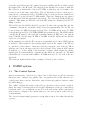
The GMRT : User’s Manual
The GMRT : User’s Manual
Dharam Vir Lal,
A. Pramesh Rao,
Manisha S. Jangam,
Nimisha G. Kantharia
.
Contents
I
Overview of the GMRT
1
1 The Array
2
1.1 Protected frequency bands . . . . . . . . . . . . . . . . . . . . . . . . .
2
2 The Receiver System
3
3 GMRT system
4
3.1 The Control System
II
. . . . . . . . . . . . . . . . . . . . . . . . . . . .
4
3.1.1
Setting RF, LO, IF and BB. . . . . . . . . . . . . . . . . . . . .
5
3.1.2
Running up correlator for recording astronomical data . . . . .
8
Before observing
14
4 Preparing for Observations
15
4.1
Spectral line observing with GMRT . . . . . . . . . . . . . . . . . . .
19
4.2 Bypass mode of 1420 MHz . . . . . . . . . . . . . . . . . . . . . . . . .
22
4.3 Dual frequency observations . . . . . . . . . . . . . . . . . . . . . . . .
22
4.4 Default parameters . . . . . . . . . . . . . . . . . . . . . . . . . . . . .
24
III
While Observing
25
5 During the Observations
26
5.1 Inputs to the operator in the GMRT Control Room . . . . . . . . . . .
26
5.2 Data quality and monitoring . . . . . . . . . . . . . . . . . . . . . . . .
27
5.2.1
IV
Total Power: . . . . . . . . . . . . . . . . . . . . . . . . . . . . .
After Observing
28
38
6 Your data
39
6.1 Interference Monitoring . . . . . . . . . . . . . . . . . . . . . . . . . . .
39
6.2 Running AIPS at the GMRT
. . . . . . . . . . . . . . . . . . . . . . .
39
6.3 Primary Beam Gain Correction . . . . . . . . . . . . . . . . . . . . . .
40
i
6.3.1
Running AIPS on your data . . . . . . . . . . . . . . . . . . . .
40
6.4 Backing your DATA . . . . . . . . . . . . . . . . . . . . . . . . . . . .
41
6.5 Your observation log . . . . . . . . . . . . . . . . . . . . . . . . . . . .
41
6.6 Computer Facilities at the GMRT . . . . . . . . . . . . . . . . . . . . .
42
6.7 Computer Facilities at the NCRA . . . . . . . . . . . . . . . . . . . . .
43
List of Tables
1
ITU specified Protected frequency bands. . . . . . . . . . . . . . . . . .
2
2
Correlator Modes . . . . . . . . . . . . . . . . . . . . . . . . . . . . . .
10
3
Bandmask for Each Mode . . . . . . . . . . . . . . . . . . . . . . . . .
11
4
Bandwidth, CLK SEL and IF selection. . . . . . . . . . . . . . . . . . .
12
5
The GMRT specifications
. . . . . . . . . . . . . . . . . . . . . . . . .
15
6
Feed description . . . . . . . . . . . . . . . . . . . . . . . . . . . . . . .
16
7
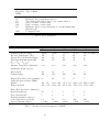
Measured System Parameters of GMRT
. . . . . . . . . . . . . . . . .
16
8
Table showing IF, baseband bandwidths and polarisation swap . . . . .
17
9
Default settings used for continuum observations for the GMRT frequency bands. . . . . . . . . . . . . . . . . . . . . . . . . . . . . . . . .
25
Primary Beam Gain Correction. . . . . . . . . . . . . . . . . . . . . . .
40
10
List of Figures
1
The block diagram of the reciever system. . . . . . . . . . . . . . . . . . .
3
2
An example of many unhealthy antennas. . . . . . . . . . . . . . . . . .
28
3
An example of a few unhealthy antennas. . . . . . . . . . . . . . . . . . .
29
4
An example of all healthy antenna.
. . . . . . . . . . . . . . . . . . . . .
30
5
An example of the ‘mon.tcl’ display.
. . . . . . . . . . . . . . . . . . . .
31
6
An example of the ‘ondisp’ display.
. . . . . . . . . . . . . . . . . . . . .
32
7
Stokes RR bandshapes of C01 & E05 and W01 & W05. . . . . . . . . .
33
8
Stokes LL bandshapes of C03 & C05, E02 & W06 and S04; in S04,
ltaflag programme has removed the spikes. . . . . . . . . . . . . . . .
34
Amplitude and phases of Primary (first) and secondary (later) calibrators on baselines with C09 (reference) and C00, C01, E02, E03 & W06.
35
Amplitude and phases of Primary (first) and secondary (later) calibrators on baselines with C09 and S02, S03, S06, W03, W05 & W06. . . .
36
9
10
11
Spectrum analyser output from optical fibre for a few of the antennas, each
plot showing 130 and 175 MHz. S06 (in left Figure) shows spikes (RFIs) in
both channels. . . . . . . . . . . . . . . . . . . . . . . . . . . . . . . . .
2
40
Part I
Overview of the GMRT
1
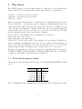
The Array
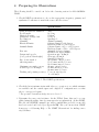
The GMRT consists of 30 45 m diameter parabolic dishes spread over 25 km near the
village of Khodad, about 80 km north of Pune, India. The site coordinates are:
latitude = 19 deg 05 min 48 sec North,
longitude = 74 deg 03 min 00 sec East,
altitude = 588 m.
The array consists of two main parts: a central array of 14 antennas which are labelled,
C# (e.g. C00, C01, ..., C14), and an outer Y consisting of 14 km long East, West, and
South arms (labelled E#, W#, and S#, respectively). There are 5 antennas on each
of the east and south arms and 6 antennas on the west arm. Note that the numbering
scheme is historical and is not consecutive; also, please note that there is no C07, E01
and S05 antennas (dropped due to the shortage of funds).
For an overview of the GMRT, telescope parameters, etc. please see
http://www.ncra.tifr.res.in
http://www.gmrt.ncra.tifr.res.in
and Section 4. It also gives details of the antenna, feed specifications, available frequencies, primary and synthesized beam sizes, and Tsys , among other parameters, are
also provided. The elevation limit of the array has currently been set to 17–90 degrees
(software limit), giving a declination range coverage from −53 to +90 degrees.
The telescope was planned to operate at 6 frequencies, but it functions at 5 frequencies,
151 MHz, 235 MHz, 325 MHz, 610 MHz, and 1000–1420 MHz. There are 4 feed systems,
of which one (235/610) is a dual frequency feed (Table 1).
1.1
Protected frequency bands
The frequency bands (shown in Table 1) are protected that fall within GMRT observing
bands.
Freq band
150.05–153
230–235
322–328.6
608–614
1400–1427
MHz
MHz
MHz
MHz
MHz
ITU
Indian
ITU
ITU
ITU
Table 1: International Telecommunications Union specified Protected frequency bands.
2
2
The Receiver System
The GMRT receivers are designed to operate at 5 frequency bands, 150, 233, 327, 610,
and 1420 MHz (the 6th, 50 MHz feed is yet to be implemented). The half-power radio
frequency (RF) bandwidth (sometimes written as BW) for 150, 235, 325 and 610 MHz
respectively is 40, 40, 60 and 100 MHz. The 1420 MHz band is split into 4 sub-bands
centred at 1060, 1170, 1280, and 1390 MHz, each with a bandwidth of 120 MHz. Thus,
the bands overlap by 10 MHz and provide continuous frequency coverage from 1000
MHz to 1450 MHz. This allows observations of HI from local gas to a redshift of about
0.4. Higher redshift HI can, of course, be detected in the lower frequency bands. The
user can also choose the full band (from 880 to 1450 MHz), this is called as the bypass
mode of 1420 band (see Section 4.2 for more details).
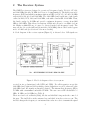
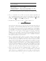
A block diagram of the receiver system (Figure 1), is shown below. RF signals are
Figure 1: The block diagram of the reciever system.
received in two polarisations (called CH1 and CH2). For all frequencies except the
1420 MHz band, right and left circularly polarised signals are received, whereas for the
1420 MHz band, the signals are linearly polarised. The intermediate frequency (IF) is
70 MHz with a maximum bandwidth 32 MHz. The user can set IF bandwidth to 6
MHz, 16 MHz, and 32 MHz (see Table 2).
There are four local oscillators (LOs), the 1st and 4th LOs being under the control of
the user. The 2nd LO is at the antenna base and third is in the receiver room. The
2nd LO changes the frequency to an intermediate value in order to transmit the signal
3
down the optical fibres into the central electronics building and the 3rd LO converts
the signal back to the IF again. The 2nd LO at the antenna base is used to shift the
IFs of the two polarisations to 130 and 175 MHz, so that they can be brought to the
receiver room on the same optical fibre. The 3rd LO in the receiver room is used to
bring the two polarisations back to 70 MHz (in the local jargon the two channels are
also referred to as the 130 and 175 MHz signal). These two channels are also termed
as the RR and LL Stokes parameters respectively. Two sidebands (USB & LSB) are
available. This makes two IFs and each of the IFs having two channels (130 and 175
MHz) or Stokes.
The 1st LO and the 4th LO should be specified (both for the spectral line and the
continuum observations, depending on the observer’s requirements). The 1st LO can
be set in steps of 1 MHz for frequencies from 150 to 354 MHz and in steps of 5 MHz
for frequencies from 350 to 1795 MHz (GMRT sub-systems report). The 4th LO which
converts the IF signal to the baseband (sometime written as BB) can be set with in
steps of 100 Hz over the range 50 MHz to 90 MHz. Both the 1st LO and the 4th LO
can be set via software.
At the antenna base, after the IF conversion, an automatic level control (ALC) system
is available. This adjusts for the varying signal levels at the output of the IF and
is controlled by the software. After the baseband conversion, each of the two IFs is
split into two bands, the upper and the lower sideband. Here again an ALC system
is available, i.e. at the output of the baseband converter, which adjusts for varying
signal levels. For interferometric observations, the ALCs are generally on. The final
bandwidth can be chosen from 64 kHz to 16 MHz in factors of 2 for each of the two
sidebands.
The baseband signal is then fed into a sampler, followed by the correlator.
3
3.1
GMRT system
The Control System
Ours is an interactive control mode so that control of the telescope and its observing
functions can be changed very quickly. Our conceptual model for this, therefore is a
control panel, where someone dials in the desired values and pushes a button to make
the whole thing go.
The “online” displays the status of the telescope (position, rates, reference position,
time), the setup of various front and back ends, information on the procedure that is
being run, and so on, on different screens. For each of the items on the control panel
there would be a display of the current value (e.g. the exact position of the telescope
at that instant).
The observer’s inputs simply generates a setup that is sent to the online through the
operator.
4
Presently, the control panel mode of program control is in its infancy. Soon, like other
observatories, we would be able to do away with a machine-readable input file and this
would update the variables. This would provide a way to design an experiment entirely
as a “real-time” operation; instead of specifying, altering various states of the control
panel; i.e. observer submits a file generated for his/her observations.
The following settings are usually done by the telescope operators.
3.1.1
Setting RF, LO, IF and BB.
Every piece of equipment including the telescope has one or more default setups, probably in the form of macros, that may be invoked with a simple command. Two or
more hierarchies of defaults are also defined to provide complete system defaults; e.g.
observing type defaults (line, continuum, pulsar, etc.), subsystem defaults, or special
purpose defaults.
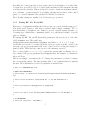
For setting the RF, LO and IF (front-end) parameters, the user needs to edit a file
called setupnew.txt. The path being
/home/operator/set/user/userx/setupnew.txt (where x = 1, 2, 3, 4, 5 or m)
for this file and can also be obtained from the telescope operators in the control room
and run a proper program which will create control word according the setting demanded in file. Then send the control word to the antennas you need.
Also, a cdsetx (where x = 1, 2, 3, 4, 5 or m) is the general purpose aliasing done to
ease editing of the proper parameter file (setupnew.txt). An example of a parameter
file is as follows:
This is an example of parameter file. To change the parameters you have to change
the corresponding entries. The lines starting with ’∗’ are comments lines for guiding
the user. More information on selected parameter is available here.
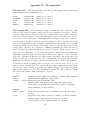
* this is a SETUPNEW.TXT file
* FRONT END PARAMETERS.
* select freq. of observation (50/150/235/325/610/1060/1170/1280/1390 MHz.)
235
* select solar attenuator (0/14/30/44 dB. -1 for FE Termination.)
0
* select polarization unswapped(0) or swapped(1).
0
* select cal-noise level.(E-HI(0)/HI(1)/MED(2)/LO(3) (-1 for RF OFF).)
1
* LO PARAMETERS.
* select LO freq.(100 - 1600 MHz.)
5
308
308
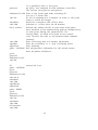
* IF PARAMETERS. (Default is 14 14)
* select pre_attenuator and post_gain for CH1. (0,2,4,...,30 dB)
16
2.5
* select pre_attenuator and post_gain for CH2. (0,2,4,...,30 dB)
16
10.2
* select IF band width for CH1 and CH2 respectively (6/16/32 MHz).
16
16
* select ALC OFF(0) or ON(1). for CH1 and CH2
0
0
* New parameters being added :
* enter NG in time domain (0,25,50 or 100) percent duty-cycle
0
* enter Walsh Enable(1) or Disable(0)
0
* Select the Walsh Group : Low Group(0) or Higher Group(1)
0
* BASEBAND PARAMETERS ( set_para[16] onwards ):
* Select the antenna group :
* [0
if all ant bb mentioned below
]
* [1
if (C0 , C1 , C2 , C3 :130 MHz)]
* [2
if (C0 , C1 , C2 , C3 :175 MHz)]
* [3
if (C4 , C5 , C6 , C8 :130 MHz)]
* [4
if (C4 , C5 , C6 , C8 :175 MHz)]
* [5
if (C9 , C10, C11, C12 :130 MHz)]
* [6
if (C9 , C10, C11, C12 :175 MHz)]
* [7
if (C13, C14, SP1, SP2 :130 MHz)]
* [8
if (C13, C14, SP1, SP2 :175 MHz)]
* [13 if (W1 , W2 , W3 , W4 :130 MHz)]
* [10 if (W1 , W2 , W3 , W4 :175 MHz)]
* [11 if (W5 , W6 , E2 , E3 :130 MHz)]
* [12 if (W5 , W6 , E2 , E3 :175 MHz)]
0
6
* Select Base BANDWIDTH in KHz (16000/8000/4000/2000/1000/500/250/125/62)
16000
* Select BB Gain (0/3/6/9/12/15/18/21/24)
0
* Select BB LO (Hz) Synth # 1 Freq.(MHz) (50.0 $<=$ LO $<=$ 90.0 $/$ step 100 Hz)
70.0000
* Select BB LO (Hz) Synth # 2 Freq.(MHz) (50.0 $<=$ LO $<=$ 90.0 $/$ step 100 Hz)
70.0000
* Select Map for BB LO Synthesizer
*
*
*
*
*
1
Chan
1
2
3
4
-
# 1
Synth
Synth
Synth
Synth
Chan
#
#
#
#
1
2
1
2
# 2
Synth
Synth
Synth
Synth
#
#
#
#
1
2
2
1
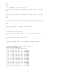
and run corresponding program which creates the control word.
ONLINE has five different user control for general purpose named user1, user2, user3,
user4 and user5. For example observer having control of user4 should use cdset4. It
creates control words for RF, LO, IF and BB in separate files which have to be sent to
the antennas and baseband systems using the following commands
>run set4rf
This will set the front end parameter according to the modification in setupnew.txt
file. If you use cdset1 to edit the parameter file then above command would be
>run set1rf
The same thing is applicable to setting LO, and IF.
To set LO and IF use the following commands.
>run set4lo
>run set4if
Setting the baseband is quiet different from setting antenna’s RF, LO or IF as the
baseband system itself is an ABC inside CEB. We have to define a different subarray
for baseband ABC, conventionally called ABC-0 (or CEB-ABC), having its ABC ID 0.
This subarray will be running all the time on ONLINE server machine and conventionally will be subarray1 (SAC1). So to change the baseband setting you have to give
commands to subarray no. 0.
The baseband is having 16 MCMs, each controlling the one polarisation and its both
sidebands for four antennas. If we send proper control word to MCM it switches the
band width and the gain according to selection.
7
Use the following command to set baseband “bandwidth”, “gain” and ’ALC’ status.
> stbbfile (130, ’default’) # gain files (130.csv)
> stbbfile(175, ’default’) # gain files (175.csv)
> stbbalc (’both’,’both’,1) # stbbalc(’130/175/both’,’usb/lsb/both’,1/0)
> stbbwgnall (16000,0) # stbbwgnall(bandwidth,gain)
> stbblo (’70.0000’,’70.0000’) # stbblo(lo4 1,lo4 2)
These commands should be run in USER0.
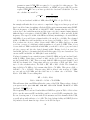
3.1.2
Running up correlator for recording astronomical data
(Based on a note by Dr. Jayaram Chengalur)
Correlator has it’s own control software which also talks to ONLINE software over
computer network. Few programs have to be run from corrletor control computer in
beginning of observation session. Then onwards control goes to ONLINE software.
Only a few commands it takes to change the source, start das, stop das and stop the
whole observing session.
For data acquisition there are two more computers involved ( mithuna - For USB &
mithunb - For LSB) which talks to correlator control PCs (corracqa - For USB, corracqb
- For LSB and corrctl - For delay traking and fringe stopping) over the network. It
creates a shared memory in it and takes the data from correlator control PC put it in
shared memory. Anyone can attach to that shared memory and get the data to display
it according to his/her convenience and to record on disk.
• INTRODUCTION:
A number of new correlator data acquisition modes are now available for test. These
modes include:
1. Full stokes (in either USB or LSB),
2. 256 channels in RR and LL (in either USB or LSB) for all baseband bandwidths
16 MHZ or smaller
3. identical data being piped through both halves of the correlator (either for possible SNR improvements, as routinely used elsewhere, or for testing)
4. In addition of course, the old ”Indian Polar” mode continues to be supported.
There has also been a substantial change in the way in which users initialize and
reconfigure the correlator and das software. Rather than having to consistently edit
several text files on several different PCs and supply consistent command line options,
users now run a single program that guides them through a menu. This program
runs on the ONLINE machine (”shivneri/lenyadri”) and produces a parameter file
8
(”/temp2/data/corrsel.hdr”). Wrappers running on shivneri/lenyadri read this file
and will initialize/reconfigure the correlator as appropriate for the selected observing
mode. Information required for configuring acq30, dlytrk etc is also taken from this
same file and transferred to appropriate locations by dassrv. This entire operation of
transfer of parameters is transparent to the user.
Step by step instructions for running the new modes, looking at the data in real time,
or offline, and converting to FITS follows:
• INSTRUCTIONS FOR RUNNING THE NEW CORRELATOR MODES:
1. log in to corracqa, corracqb, corrctl as observer, chose the ”d” (”dvl”) when
prompted for which software system to use. (This sets the paths and environment
variables appropriate for the new ”development” software. NB: if there are any
shared memories floating around from the older das versions, you will need to
delete them).
2. login in to mithuna and mithunb as observer and chose ”d” when promoted
for which software system to use. (Again, this sets the paths and environment
variables appropriate for the new ”development” software. NB: if there are any
shared memories floating around from the older das versions, you will need to
delete them).
3. login into shivneri/lenyadri as observer, and cd to /home/observer/dassrv-dvl If
you want to initialize the correlator, run
> corr init on *shivneri/lenyadri* (This will run corr config and newdly config
on the corrctl PC).
4. Choose the observing setup by running > corrsel
on *shivneri/lenyadri*
(This will setup the file /temp2/data/corrsel.hdr, which contains information on
how you want the correlator configured. corrsel allows a menu based selection of
the observing mode, integration time, clksel etc.
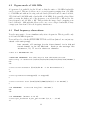
At the moment, the following modes are predefined in corr sel:
The names are hopefully self explanatory.
In addition, you can configure a vast number of modes by editing the DPC MUX
and MAC MODE fields in the corrsel.hdr file.
The valid MAC MODE values are RRLL RRRL and RR
The valid DPC MUX values are any of the strings:
IndianPolar, UsbPolar, LsbPolar, UsbCopy, LsbCopy,
AllU130, AllU175, AllL130, AllL175,
arar\_arar, alal\_alal, brbr\_brbr, blbl\_blbl,
aral\_brbl, aral\_alar, brbl\_blbr, arbr\_albl,
9
/* new modes */
/* historical */
0
1
2
3
4
5
6
7
8
9
10
Corr Mode
IndianPolar
UsbPolar
LsbPolar
UsbHighRes
LsbHighRes
UsbCopy
LsbCopy
AllU130
AllU175
AllL130
AllL175
Table 2: Correlator Modes
Again the names should be self explanatory. In addition, the mode can be a string
of the form dpc abcd, where 0¡= a,b,c,d ¡=3. A mode of the form dpc abcd means
that the dpc mux sends channel a data to where channel 0 data normally goes,
channel b data to where channel 1 data normally goes and so on.)
NB: In the UsbHighRes and LsbHighRes modes the DPC MUX is set to UsbPolar
and LsbPolar respectively. However the MAC MODE will defer for the HighRes
and Polar modes.
5. reconfigure the correlator to the selected mode. To do this type
>corr reconf
on *shivneri/lenyadri*. PLEASE NOTE THAT IF YOU ARE CHANGING
THE MODE, IT IS NECCESSARY TO DO A hltndasc AND RESTART acq30
ETC. (IT MAY BE SAFEST TO KILL AND RESTART ALL THE acq PROGRAMMES. NOT KILLING acq MAY AFFECT SYNCHRONIZATION OF
THE TWO PIPELINES. MOST OF THE TIME IT SHOULD BE FINE TO
KEEP acq RUNNING, AND JUST CHECK FOR SYNCHRONIZATION PROBLEMS AFTER YOU RESTART. IF THINGS ARE SYNCHRONIZED THEN
FINE, OTHERWISE YOU WILL NEED TO KILL AND RESTART acq).
6. start acq, acq30, sockcmd fstop, dlytrk,dassrv,collect on the appropriate machines. Note that none of the programs need command line options, but instead,
as explained in the introduction, will automatically understand the selected observing mode.
NB: The acqs on corracqa/corracqb/corrctl should be started within 1 STA cycle(i.e. 128 ms!) of each other. The easiest way to do this is:
10
Mode Name
IndianPolar
UsbPolar
LsbPolar
UsbHighRes
LsbHighRes
UsbCopy
LsbCopy
AllU130
AllU175
AllL130
AllL175
Band Mask
15
3
12
3
12
3
12
1
2
4
8
Table 3: Bandmask for Each Mode
(a) export the corracqa/b/ctl window to all desktops.
(b) go to any one desktop and align the acq windows one below the other
(c) type ”acq” in all windows (but don’t type ENTER!)
(d) hit the ENTER button in all windows in quick succession.
I agree that this is a pretty silly way to do things. A more automatic method is
in the prorverbial pipeline.
7. Ask the operator to give an init and add a project from the master terminal. The
bandmask while initing and adding a project should be correspond to the chosen
mode.
NB: The bandmask is a bit mask with bits in the order USB130 USB 175 LSB130
LSB175
For a pure USB observation the bandmask is 3 (e.g. UsbPolar, UsbCopy, AllU130..)
For a pure LSB observation the bandmask is 12 (e.g. LsbPolar, LsbCopy, AllL130..)
For a dual sideband observation the bandmask is 15 (e.g. IndianPolar).
The actual bandmask for each mode is tabulated below:
NB: All of these modes use both halves of the correlator, so will use CMODE 3
in ONLINE.
8. start and stop scans, record as usual. Median filter can be used. as always it is
upto the user to decide if s/he wants median filter or not. The maximum filter
length is 128. RECORD NOW TAKES AN ADDITONAL OPTION ”SELF”.
IF THE LAST [OPTIONAL] ARGUMENT IS ”SELF” THEN RECORD WILL
PUT ONLY THE SELF CORRELATIONS IN THE LTA FILE. For example.
11
Bandwidth
(MHz)
Samp freq
(MHz)
Samp rate
(µ sec)
CLK SEL
Channel width
(kHz)
16
8
4
2
1
0.5
32
16
8
4
2
1
0.03125
0.06250
0.12500
0.25000
0.50000
1.00000
0
1
2
3
4
5
125.0
62.5
31.25
15.625
7.8125
3.90625
Possible IF-BW
(MHz)
32/16
32/16 (6 ?)
32/16/6
32/16/6
32/16/6
32/16/6
Table 4: Bandwidth, CLK SEL and IF selection.
> record TEST test.lta 8m self
will create a file test.lta with only self correlations in it.
NB: In the new modes the data is divided between the two halves of the correlator.
For example in the UsbPolar mode U130xU130 and U175xU130 come in mithunb
(i.e. the ”ltb” file) while U175xU175 and U130xU175 come in mithuna (i.e.the
”lta” file). Hence
(a) dasmon in mithuna or mithunb will only show you one half of the data
(b) ”normalization” cannot be applied in some modes. To normalize U175xU130
one needs the U130 and U175 selfs, but both will be available only when
one merges the data streams.
9. . You can merge the lta and ltb files using ltamerge. This merged file will have
the complete data, and is easier for playing around with taxx.
10. The merged file can be converted to FITS using listscan and gvfits. These programs are also backwards compatable. The individual lta/b files can also be
converted using these programs, but I don’t seem to be able to get AIPS to
understand the polarizations in a file with only RR RL or only LL LR. I think
that only some partitioning produced by the VLA correlator is understood. The
combined RR RL LR LL FITS file is interpreted without problem.
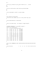
• In (online machine) User0 window
>cmode 3
1 for USB, 2 for LSB, 3 for both
>tpa(11)=15
>allant
puts all 30 antennas in array
>initndas ’/temp2/data/corrsys.hdr’
12
>suba 4
subarray number for which project is to be started
>prjtit’title’
The title for the project, upto 80 characters.
>prjobs’Yourname’
‘TST’ or Name of Observer, upto 8 characters.
>ante 10 1 2 3 .... 10 or allant
>initprj(15,’PRJCODE’)
3 for USB, 12 for LSB, 15 for both
• From User4 of online
>tpa rf1 rf2 lo11 lo12 lo41 lo42
Here rf is the frequency of the band edge ( channel 0), lo1 is the frequency of the first
local oscillator, lo4 is the frequency of the fourth local oscillator.
e.g. tpa 325 325 255 255 70 70. See Sections 4 and 4.1 for more information.
>prjfreq
Copy project parameters into ONLINE shared memory
>lnkndas
Setup the link between ONLINE and DAS.
>gts ’srcname’
Get source parameters.
>sndsacsrc(1,12h)
Position antennas to the source and begin tracking.
>strtndas
Start the data acquisition for the given source.
>stpndas
Stop the data acquisition for the given source.
>opsacfil ’/odisk/gtac/cmd/yourname.cmd’
To open the Sacfile or Command file.
>strtsacfil
It gives control to the subarray controller which reads the instructions from above
mentioned file (yourname.cmd).
>stpsacfil
Stop the command file (yourname.cmd).
• From User0 window of online
>cmode 3
1 for USB, 2 for LSB, 3 for both
>suba 4
subarray number for which project is to be started
>stpprj
Stop the project.
>hltndas
Halts acquiring the data from correlator.
13
Part II
Before observing
4
Preparing for Observations
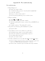
The following should be carried out before the observing session for ALL OBSERVATIONS.
1. Check GMRT specifications to choose the appropriate frequency, primary and
synthesized beam sizes to match the source and the science.
Specifications
Parabolic Reflector Diameter
Focal Length
Physical aperture
Sensitivity of single dish
Feed Support
Mounting
Elevation Limits
Azimuth Limits
Slew rate
Design wind speeds
(3 sec peak at 10 m height)
Size of wire mesh of
reflecting surface
Maximum rms surface errors,
at wind speed of 40 kmph
Tracking and pointing accuracy
45m
18.54 m
1590 m2
0.3 K/Jy
Quadrupod
Altitude-azimuth
Software Limit 17−90 degrees
Hardware Limit 15−110 degrees
Software Limit −265 to +265 degrees
Hardware Limit −270 to +270 degrees
Azimuth 30 degree/minute
Elevation 20 degree/minute
Operation upto 40 km/h
Slew upto 80 km/h
Survival 133 km/h
20×20 mm, outer 1/3 area
15×15 mm, middle 1/3 area
10×10 mm, inner 1/3 area
20 mm, outer 1/3 area
12 mm, middle 1/3 area
08 mm, inner 1/3 area
10 rms at wind speeds
of < 20 km/h
Table 5: The GMRT specifications
2. Check the latest antenna status with telescope operators to see which antennas
are available and the central square and complete Y configurations to see that
the uv coverage is adequate.
* For spectral observations fudge factor is close to 1
3. Determine the source rise/set times. At the NCRA, Pune, this can be accomplished using the utility, tact (see man tact for an explanation). At the GMRT,
Khodad, the ONLINE command ‘gts’ will accomplish this, provided a source file
has been created and loaded (see Appendix Z2). Also you can use from ’GMRT
home-page → Observing Help → For GMRT Observations’ for finding source
rise/set times.
15
Frequency
(MHz)
Type of feed
50
153
233
610
327
Half-wave dipole with linear reflector
Two Orthogonal pairs or dipole over a plane reflector
Dual concentric coaxial cavity
Dual concentric coaxial cavity
Half-wave dipole over ground plane & a beam-forming ring
(Kildal feed)
Corrugated horn
1420
Table 6: Feed description
Primary Beam (arc min)
Receiver Temperature (TR )
Typical Tsky (off Galactic plane)
Total System Temperature (K)
(TR + Tsky + Tground )
Antenna Temp (K/Jy/Antenna)
151
186±6
144
308
482
235
114±5
55
99
177
Frequency (MHz)
325
610
81 ± 4
43 ± 3
50
60
40
10
108
92
0.33
0.33
0.32
0.32
0.22
Synthesised Beam (arcsec)
Whole Array
Central Square
20
420
13
270
9
200
5
100
2
40
68
44
32
17
7
Largest Detectable Source(arcmin)
Usable Frequency Range (MHz)
Reliable
With some Luck
Fudge Factor(actual to estimated)
Short Observations
Long Observations*
Best rms sensitivies achieved
so far as known to us (mJy)
Typical Dynamic Ranges
1420
24 ± 2 ∗ (1400/f )
40
4
76
150 - 156
232 to 244 315 to 335 590 to 630 1000 to 1450
150 to 158 230 to 250 305 to 360 570 to 650 950 to 1450
10
5
5
2
2
2
2
1
2
1
1.5
> 1000
0.6
> 1000
0.3
>1500
0.02
>1500
0.03
>2000
Table 7: Measured System Parameters of GMRT
16
System Settings
IF bandwidths
Baseband bandwidths
Polarisation swap
32, 16, 6 MHz
16, 8, 4, 2, 1, 0.5, 0.25, 0.12, 0.062 MHz
Swap on (1) / Swap off (0)
Table 8: Table showing IF, baseband bandwidths and polarisation swap
4. Choose a bandwidth, ∆ν (see Table 2), from the available bandwidths and
choose a sampling frequency which is twice the bandwidth (for Nyquist sampling). The sampling frequency is specified via the parameter, clk sel, where
2 × BB = samp freq = 32/(2clk sel ) (see Table 4).
5. Determine the required time on source, τ . This is computed via:
√
2 k Tsys
q
∆S =
ηa ηc A (nb ) nIF ∆ν τ
where ∆S is the required rms noise (Jy), Tsys is the system temperature (K), and
[(ηa A)/(2k)] = G is the antenna gain (K/Jy), where ηa and ηc being aperture
and correlator efficiencies respectively. A is the geometrical area of the antenna,
nb is the number of baselines, nIF is the number of IF channels, and ∆ν (Hz) is
the bandwidth of each sideband (or channel width for spectral line observations).
Here, nIF = npol + nSB , where npol is the number of polarisations (2 for the
GMRT) and nSB is the number of sidebands. Note that the improvement in S/N
by operating in double sideband mode applies only to continuum observations.
The required parameters are provided here.
6. Choose a primary flux density calibrator and phase calibrator from the VLA
calibrator manual. The VLA calibrator manual is also available at the GMRT
site. The best sources for GMRT use will be those which are usable at all VLA
arrays (A, B,C, and D). However, sources which are not acceptable as A array
calibrators (and possibly B) may still be acceptable, provided the appropriate
uv limits are adhered to. It is best not to use a calibrator which is not usable at
D array since this will eliminate the central square of the GMRT. Decide which
calibrator will be used to calibrate the bandpass. This is usually the flux density
calibrator, but could be the phase calibrator for strong, low frequency sources.
7. Create a source file; the source file contains the names, coordinates, and coordinate epochs of all sources to be observed. It is usually named via the initials
of the observer (e.g. ‘yourname.list’, lower case !). Only one such file is usually necessary (a master list) since the file can contain more sources than are
17
actually observed. The format must be exact (including spaces) and is case sensitive. Thus, it is best, when first making the file, to copy and edit one which
is already in existence. The telescope operator can supply a template file (or
see astro1@lenyadri/shivneri/lenyadri:‘/odisk/gtac/source/?.list’). There is
already a ‘cal.list’ file in regular use which includes many calibrator sources,
including the primary VLA flux density calibrators. However, it does not contain all sources in the VLA calibrator manual. Therefore, it is likely that the
phase calibrators will also need to be included in the user’s master list of sources.
Once the source file is created in the user’s home directory, it should be copied
by the telescope operator into a directory which can be read during the observing session. A sample ONLINE command for loading the file is addlist
astro1:lenyadri/shivneri/lenyadri:/odisk/gtac/source/yourname.list.
8. Create a command file (see Appendix Z2 in the end of this document and/or
astro1@lenyadri/shivneri/lenyadri:‘/odisk/gtac/cmd/?.cmd’ for templates). This
file contains commands for the telescope to slew to a source, track, collect data for
a specified time, etc. Any of the commands in this file can also be input manually
at the console during observations, but the file, when accessed, will prevent the
necessity of a continuous input of manual commands. It is possible to override
this file from the console; however, when started again, it will start from the beginning of the file, so some editing might be required if this occurs. Strategically,
it is best to start the observing run with commands issued manually so as to monitor a calibrator and correct problems from the console level, if they occur. Once
satisfied, the command file can then be invoked. A typical example of a command
file can be found in Appendix Z2. Command files are usually put in the directory, e.g. astro1@lenyadri/shivneri/lenyadri:‘/odisk/gtac/cmd/yourname.cmd’
(lower case !).
9. Choose a integration time. The integration time specifies the time over which
data from the source is collected, thus specifying the time interval for an individual visibility. The integration time is specified through the parameter, LTA (long
term accumulator), which is an integral number of STA (short term accumulator)
units, the latter being the shortest sampling time allowed by the correlator. One
STA = 132.096 milliseconds, so LTA = 128 corresponds to 16.908 seconds. If a
10 minute scan is specified, there would be ∼ 35 record ((60 × 10)/16.908) points
in your datafile.
10. Choose the BB bandwidth (see Table 2). The BB should be at least as large as
the final IF width, but much larger could introduce unwanted interfering signals.
11. Choose a sideband and determine the frequency of the 1st LO. For lower sideband
(LSB) operation, νLO1 > νRF and νLO1 − νLO4 = νRF , where νLO1 is the local
oscillator frequency, νLO4 = 70 MHz is the IF, and νRF is the sky (observing)
frequency. For upper sideband (USB) operation, νRF > νLO1 and νRF − νLO4 =
νLO1 . The tuning is set to match the 1st channel, not the centre of the band and
18
the user should note the permitted frequency increments (see Section 2). Also
note that there may be other technical considerations which limit which sideband
can be used at any time. The user should check with a local expert. The user
can also use the programme tune available locally.
4.1
Spectral line observing with GMRT
This section is for users interested in spectral line observations with GMRT. Observer
must be aware that GMRT always observes in the spectral line mode. The FX correlator always generates 128 channels per sideband for the selected baseband bandwidth.
This is useful since one can take care of bandwidth smearing and also fixed delay effects
across the band. What differentiates spectral line observations from standard continuum observations is that the local oscillator settings are important so as not to miss the
spectral line which is expected at a certain frequency. For the continuum observations,
one can use the default settings (see Table 9) for the desired band. Moreover, one can
choose to record less than 128 channels in the case of continuum observations whereas
for spectral line projects, recording data of all channels would be desirable.
For spectral line projects, the user will need to have an idea of the observing frequency
and the desired bandwidths.
1. Determining the observing frequency: Once you know the rest frequency
of your spectral line, the redshift for far Universe objects should give you the
observing frequency. In case of Galactic or near Universe objects, the NRAO
programme ’dopset’ (available via usual “source /astro/RC”) can be used to
obtain the change in the rest frequency due to the earth’s rotation and motion
around the Sun so as to obtain the heliocentric or the local standard of rest
values. Please note that online Doppler correction is not provided at GMRT the change over an eight-hour run is ∼1 km/s.
2. Determining the baseband bandwidth: The available bandwidths at GMRT
are in binary steps from 62 kHz to 16 MHz. Observations with bandwidths greater
than 0.5 MHz are regularly made whereas the lower bandwidths are not frequently
used. You will have 128 channels spread over the baseband bandwidth that you
choose. Please note that there are three choices for the IF bandwidth: 6, 16 and
32 MHz. Depending on your project, the line width will vary from a few km/s
(Galactic lines) to a few hundred km/s (extragalactic lines). Select a channel
width such that you have at least 2-3 channels across your expected line width.
Thus ‘128×selected channel width’ gives you a ‘minimum’ bandwidth required.
The other point to consider now is the desired velocity coverage. This is also
very project dependent. If you are trying to observe multiple transitions within
your band e.g. while observing recombination lines, it is desirous to obtain both
hydrogen and carbon lines which are separated by 150 km/s within the band.
Thus, this might mean compromising your channel width. This is a subjective
19
decision. The third and last part is the available bandwidths at GMRT. You have
to make your own decision as to which is the best combination for your project.
In the new correlator modes you could have 256 channels (see section 3.1.2 and/or
GMRT home-page → Observing Help → Features in the Experimental Stage).
3. Determining the LO settings: Once you have decided on your observing
frequency and the baseband bandwidths, you need to figure out the local oscillator
settings for GMRT. For Galactic and near Universe spectral line observations,
fine adjustments to the local oscillator frequencies are required for the narrow
bandwidths used. For the distant Universe, these settings are more coarse since
the bandwidths generally employed are large. To help you with these settings
a locally developed programme tune is available at GMRT. The programme is
user-friendly and will help you play around with the local oscillator frequencies
(both for LO1 > RF and LO1 < RF). Default settings are as follows:
150 MHz
240 MHz
330 MHz
610 MHz
L sub-bands
LO1
LO1
LO1
LO1
LO1
>
>
<
<
<
RF
RF
RF
RF
RF
and visualize your observing band. It also provides you with default local oscillator settings for each GMRT frequency band used for continuum observations.
Please note that LO1 (the first local oscillator in electronics) has a least count
of 1 MHz for frequencies < 350 MHz and a least count of 5 MHz for frequencies
> 350 MHz. This translates practically to the fact that only coarse settings are
possible in the LO1 whereas the fine settings have to be implemented using LO4
(the fourth LO in the electronics). Only LO1 and LO4 are under user control
since LO2 and LO3 are used for optical fibre transmission from the antennas base
to the receiver room. Once you have determined all the required frequencies, you
can use the Frequency Setting Calculator on the GMRT web-page to determine the array of parameters tpa which are required by the correlator. The TPA
array consists of 6 members namely as follows:
RFfreq in spec chan 1 for 130 MHz ,
RFfreq in spec chan 1 for 175 MHz ,
LO1for 130 MHz ,
LO1for175 MHz ,
LO4for130 MHz ,
LO4for175 MHz
where 130 MHz corresponds to RR and 175 MHz to LL polarisations. Please
note that (RFfreq ± LO1 = LO4). If you plan on dual frequency observations
ie 240 MHz on LL and 610 MHz on RR (default), you will follow the explanation discussed just above. In addition to the above, depending on your baseband bandwidth you will need to tell the correlator the sampling frequency. A
20
parameter named CLK SEL is required to be specified for this purpose. The
Frequency Setting Calulator avaliable on GMRT web-page will tell you the
required CLK SEL once you have specified the baseband bandwidth. You can
also calculate it yourself as
2CLK
SEL
=
16
.
(baseband BW)
So if your baseband width is 8 MHz, then CLK SEL = 1 (see Table 4).
An example will make the above easier to comprehend. Suppose we have proposed and
have been alloted time for making a Galactic HI absorption measurement using GMRT.
The rest frequency of the HI line is 1420.40575 MHz. Assume that the velocity correction due to the earth/Sun motion and the source velocity (computed using dopset)
shifts the line to a frequency of 1420.505 MHz. We would like to center our band on this
frequency. The expected width of the HI line is 10 km/s translating to about 48 kHz at
1400 MHz. So we would desire a channel width of about 48/4 = ∼12 kHz. For a channel
width of 12 kHz, the total bandwidth you can observe is (12 kHz × 128) = 1.5 MHz.
Now you have two choices - either observe with 1 MHz or 2 MHz. Suppose you want
a velocity coverage of ∼200 km/s which translates to about 0.95 MHz. Thus, if you
observe with a 1 MHz bandwidth at 1400 MHz, you should be able to get your desired
velocity coverage and also the desired channel width. Having decided on your basebandwidth, lets try to determine the LO1 and LO4 required by your observations. You
can use an IF bandwidth of 6 MHz (the lowest available).
You have determined your central frequency (1420.505 MHz) and your baseband bandwidth (1 MHz). Using these you have to find out the local oscillator settings. Let’s
use the default LO1 < RF. Then you want 1420.005 MHz in spectral channel 1 and
1421.005 in channel 128. Using tune will give you values of LO1 and LO4. Let’s
try to do the calculation here. For LO1 < RF, RF = LO1 + LO4. The default setting for LO4 is 70 MHz so let’s assume that LO4 = 70 MHz. This gives a LO1 =
1420.005 − 70 = 1350.005. However since LO1 is allowed only in steps of 5 MHz,
we can only set 1350 MHz and the 0.005 has to be taken care of in LO4. Thus
LO4 = 1350 MHz. Now recalling that
RF = LO1 + LO4;
LO4 = 1420.005 − 1350.0 = 70.005MHz.
This will ensure that your HI line falls in the center of the USB. Thus you have obtained
your tpa as under, tpa 1420.005 1420.005 1350 1350 70.005 70.005 For 1 MHz
baseband, CLK SEL = 4.
The frequently used baseband bandwidths at GMRT are given in Table 4. It is advisable to use the narrowest IF bandwidth possible so as avoid RFI corrupting the data.
For an observing run of 9 hours with all 30 antennas and 128 channels in the USB,
you will end up with a filesize of > 2 GB. The data backup facility at GMRT (Section
6.4) includes several 4mm dat tape drives for 24 GB dat tapes.
21
4.2
Bypass mode of 1420 MHz
A bypass mode is available for the L band so that the entire ∼ 500 MHz bandwidth
can be accessed. This mode allows one to access frequencies ranging from 850 MHz
to 1500 MHz and without choosing each sub-bands (each sub-band is centred at 1060,
1170, 1280 and 1390 MHz with a bandwidth of 120 MHz). It is generally advised that
while accessing the higher end of the frequency, you set the LO1 > RF and for the
lower frequency end set LO4 < RF. This prevents the image band corrupting your
band of interest. Although this allows you to use cover a larger bandwidth, it may
corrupt your data from local radio frequency interference.
4.3
Dual frequency observations
You also may want to observe simultaneously at two frequencies. This is possible only
at 233 and 610 MHz frequencies.
You would need to edit the SETUPNEW.TXT file as follows (instead one can just say
cdsetd on the unix-prompt):
here onwards, all settings for the first channel is for 610 and
second channel is for 235 MHz band. Watch on the settings like
attenuator, LO, IF etc for these two channels.
* this is a SETUPNEW.TXT file
* FRONT END PARAMETERS. Give 1420 only for full 1420 band selection.
*select freq. of observation (50/150/235/325/610/1060/1170/1280/1390/1420MHz.)
610
235
* select solar attenuator (0/14/30/44 dB. -1 for FE Termination.)
0
14
* select polarisation unswapped(0) or swapped(1)
0
* select cal-noise level.(E-HI(0)/HI(1)/MED(2)/LO(3) (-1 for RF OFF).)
0
* LO PARAMETERS.
680
310
* select LO freq.(100 - 1600 MHz.)
* IF PARAMETERS. (Default is 14 14)
* select pre_attenuator & post_gain for CH1.(0,2,4,...,30 dB)
12
22
12.3
* select pre_attenuator & post_gain for CH2.(0,2,4,...,30 dB)
18
18.5
* select IF band width for CH1 & CH2 resp.(6/16/32 MHz).
32
32
* select ALC OFF(0) or ON(1). for CH1 and CH2
1
1
* New parameters being added :
* enter NG in time domain (0,25,50 or 100) percent duty-cycle
0
* enter Walsh Enable(1) or Disable(0)
0
* Select the Walsh Group : Low Group(0) or Highr Group(1)
0
* BASEBAND PARAMETERS ( set_para[16] onwards ):
* Select the antenna group :
* [0
if all ant bb mentioned below
]
* [1
if (C0 , C1 , C2 , C3 :130 MHz)]
* [2
if (C0 , C1 , C2 , C3 :175 MHz)]
* [3
if (C4 , C5 , C6 , C8 :130 MHz)]
* [4
if (C4 , C5 , C6 , C8 :175 MHz)]
* [5
if (C9 , C10, C11, C12 :130 MHz)]
* [6
if (C9 , C10, C11, C12 :175 MHz)]
* [7
if (C13, C14, SP1, SP2 :130 MHz)]
* [8
if (C13, C14, SP1, SP2 :175 MHz)]
* [13 if (W1 , W2 , W3 , W4 :130 MHz)]
* [10 if (W1 , W2 , W3 , W4 :175 MHz)]
* [11 if (W5 , W6 , E2 , E3 :130 MHz)]
* [12 if (W5 , W6 , E2 , E3 :175 MHz)]
0
* Select Base BANDWIDTH in KHz (16000/8000/4000/2000/1000/500/250/125/62)
16000
* Select BB Gain
0
(
0/
3/
23
6/
9/
12/ 15/ 18/ 21/ 24)
* Select BBLO (Hz) Synth # 1 Freq.(MHz) (50.0 <= LO <= 90.0 , step 100Hz)
66.0000
* Select BBLO (Hz) Synth # 2 Freq.(MHz) (50.0 <= LO <= 90.0 , step 100Hz)
66.0000
* Select Map for BB LO Synthesizer
*
*
*
*
*
3
Chan
1
2
3
4
-
# 1
Synth
Synth
Synth
Synth
Chan
#
#
#
#
1
2
1
2
# 2
Synth
Synth
Synth
Synth
#
#
#
#
1
2
2
1
Now run
>setdlo
>setdif
>setdrf
etc.
tpa to be given is 614 244 680 310 66 66.
Record 64 channels (needs to be mentioned in corrsys.hdr file and look at the bandshape from the showband.tcl programme; 0,63,1). Check with MATMON and also check
DASSTAT window.
After the observation you can convert your data in FITS using gvfits. Use the “gvfits”
programme as follows:
astro1> listscan /rawdata/7jun/01TST01_OBJ.lta
astro1> vi 01TST01_OBJ.log
astro1> gvfits 01TST01_OBJ.log
For examples, editing 01TST01 OBJ.log suggests to keep one of the stokes, say RR (also
important is to choose normalisation/unnormalisation !). The output ‘TEST.FITS’
would correspond to one of the frequency data (614 MHz) and re-run “gvfits” for the
other stokes (i.e. LL, 240 MHz) data.
4.4
Default parameters
The default settings used for continuum observations for the GMRT frequency bands in
terms of RF, LO1, LO4 frequency settings, Solar Attn (in dB) and IF, BB bandwidths
(all in MHz), ALC Status are shown in the Table 9.
24
Freq Solar RF 130 RF 175 LO1 130 LO1 175 LO4 130 LO4 175
band Attn
RR
LL
RR
LL
RR
LL
150
14
157
157
223
223
66
66
235
14
244
244
310
310
66
66
325
0
325
325
255
255
70
70
610
0
610
610
540
540
70
70
1060
0
1060
1060
990
990
70
70
1170
0
1170
1170
1100
1100
70
70
1280
0
1280
1280
1210
1210
70
70
1390
0
1390
1390
1320
1320
70
70
dual 0-14
614
244
680
310
66
66
IF BB ALC
BW BW
6
8
ON
6
8
ON
32
16
ON
32
16
ON
32
16
ON
32
16
ON
32
16
ON
32
16
ON
32-6
8
ON
Table 9: Default settings used for continuum observations for the GMRT frequency
bands.
Part III
While Observing
5
During the Observations
The information which has previously been obtained during the preparation (Section
4) stage is now brought to and applied during observations. Aside from the source
file and the command file which the user must prepare in advance, the other information can be provided to the telescope operators (“observers”) during set-up. It is the
user’s responsibility to ensure that the observational set-up is correct, however, so it is
important to monitor and check each step of the set-up and observing operations.
There are several other files, at this point, of which the user should be aware and which
the telescope operator will edit according to user specifications.
One file is called setupnew.txt which sets up the hardware. Specified in this file are
the observing frequency, front end parameters, the 1st LO, the IF bandwidth and the
final baseband bandwidth (see also Section 2).
The other file of interest to the user is the corrsys.hdr file. This file contains the LTA
(Section 4) value and channel selection.
The user should also check that the ALC (Section 2) switches are on.
As the telescope operator sets up the session, the user should particularly check the
command, e.g. tpa 1418 1418 1350 1350 68 68. This specifies the sky frequency for
both polarisations (1st and 2nd numbers), the 1st LO frequency for both polarisations
(3rd and 4th numbers), and the 4th LO frequencies for both polarisations (5th and 6th
numbers).
As the visibilities are recorded, the user should check on the amplitude of the signals
from the calibrators. For self-correlations, the amplitudes should be, the correlation
coefficients, i.e.
Tant
A =
Tant + Tsys
where Tant = S×G; S, the source flux density (Jy), G, the gain (K/Jy) and Tsys the
system temperature (K). Refer to Tables above in Section 4 for system values. These
correlation coefficients are shown on the MATMON window (see Section 5.2.1–?? for
examples of real-time display of cross-correlation outputs on a MATMON window).
Finally, information on troubleshooting is provided in the end (Appendix Z3).
5.1
Inputs to the operator in the GMRT Control Room
A file (via email or personally) with the following inputs:
From: Your Name
To: The GMRT control room
The settings are :
Source
: OBJECT
26
ProjCode
Phase Cal
Flux Cal
:
:
:
:
01TST01
phas_cal
3C48 (before the command file)
3C147 (after the command file)
Command file : /odisk/gtac/cmd/yourname/yourname.cmd
Source list : /odisk/gtac/source/yourname.list
Settings :
---------------------------------------BAND
= 1280 MHz
LO1
= 1215 MHz
LO4
= 74.6 MHz
IF
= 16 MHz
BB
= 1 MHz
CLK_SEL
= 4
tpa 1289.6 1289.6 1215 1215 74.6 74.6
Note:
Please observe 3C48 for 20m before the target source rises
and observe 3C147 for 20m after the target source sets.
Use LTA2=8m (for 16sec integration)
The CLK SEL for various baseband frequencies are given in Table 4, it can also be
found using
samp freq
baseband BW =
2
and
32
samp freq = (clk sel) .
2
5.2
Data quality and monitoring
The purpose of on-line data monitoring is to provide a running check on data integrity
and proper operation of the system. User and operator interaction is limited to selecting
the type and options of the display appropriate to the data being collected plus some
scroll-back through the most recent displays.
Although, the telescope operators are fairly helpful during the observations and knowledgeable, it is the user who is responsible for ensuring that the observatinos run
smoothly and correctly. The telescope operator is responsible only for seeing that the
data are collected with apparently functioning equipment. The observer is responsible
for the ultimate quality of the data, its calibration, and so on.
The displays (say for USB) that have proved useful so far to review the recent history
of system temperature, gain, and total power level. A few of these are outlined below.
27
5.2.1
Total Power:
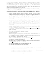
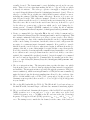
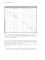
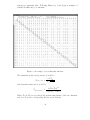
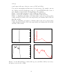
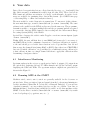
Figure 2: An example of many unhealthy antennas. The values along the diagonal show the
values of the self-correlation-coefficients, the upper-trangular-half show the cross-correlationcoefficients for the 130 MHz channel and lower-trangular-half show the cross-correlationcoefficients for the 175 MHz channel.
The total power (or system temperature, when ALC is off) is the single most important
diagnostic of the status of the observations. It contains information on everything
from elevation to interference to the weather. Display of total receiver power or system
temperature is useful for all types of observing.
Several software are available to examine the data in the lta format. Some of them are
discussed below:
1. dasmon The monitoring needed for continuum observations are largely given by
the dasmon. dasmon is a snapshot mode of getting a quick health check of the
28
system at a particular time. Following Figures (2, 3 and 4) gives examples of
available healthy and poor antennas.
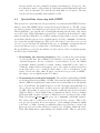
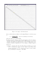
Figure 3: An example of a few unhealthy antennas.
The sensitivity in the total power mode would be
Ttotal
power
∝
2 k Tsys
√
A ∆ν τ
and in interferometric mode would be
Tinterferometric ∝
0
k (Tsys Tsys
)1/2
√
.
2 (A A0 )1/2 ∆ν τ
0
Where Tsys & Tsys
are repectively the system temperatures of the two antennas,
0
and A & A are the corresponding effective areas of them.
29
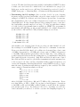
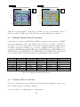
Figure 4: An example of all healthy antenna.
Cross-correlation functions displayed on the dasmon (Figures 2, 3 and 4) are given
by
S(in Jy) × K
ccf ∝
, where K is sensitivity and is in K/Jy;
Tsys
with some scaling factor (usually 1000).
Each Figure shows the following: (i) the diagonal elements are the self-correlationcoefficients, (ii) the upper-half elements are the 130 MHz channel cross-correlationcoefficients and (iii) the lower-half elements are the 175 MHz channel crosscorrelation-coefficients. Explanations for a few examples of dasmon outputs is
given below:
(a) Figure 2: Antennas C02, C05, C13, E01, S01 S05 and W04 were not avaliable for observations (see empty rows and columns corresponding to these
antennas in the Figure 2). The observations were made on source 3C468.1
(project 01TST01) at a frequency of 1060 MHz.
30
(b) Figure 3: Here all the antennas were used for the observations. The C04,
E04, S01, W03 and W04 were down at both polarisations, whereas S04 and
W02 (may be W01 as well !) was down in one polarisation only (either 130
or 175 MHz). The observations were made on source 3C147 source.
(c) Figure 4: Something that an astronomer would love to see. This is an
example where all antennas are healthy. User should compare the crosscorrelation shown in this figure (Figure 4) with the one that is theoretically
expected using above relation.
dasmon also allows (see Figure 5 below) the user to continuously monitor the
amplitude and phase of the source being observed. For the sophisticated user,
this is fairly useful in determining the stability of amplitude and/or phase. i.e.
especially during scintillation and fringe winding.
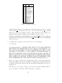
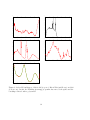
Figure 5: An example of the ‘mon.tcl’ display.
2. ondisp
Task ‘ondisp’ (see Figure 6) allows a user to keep track of antennas which are in
healthy state. Each antenna shows a ‘flag’ associated with it. A few of the key
‘flags’ means as follows:
t
b
w
: time out
: brake
: wind
Z
B
m
: slewing
: azimuth brake
: mcm (monitor & control module) time out
3. tax
Task to extract data from a GMRT LTA file, with optional averaging in time
and selection on time, baselines, frequency channels and on scans via the object
name and/or scan number.
{astro0}> tax
tax> in
tax> scans
= /rawdata/8jun/01TST01.lta
= 0,1,2
31
Figure 6: An example of the ‘ondisp’ display.
tax>
tax>
tax>
tax>
tax>
tax>
tax>
tax>
tax>
object
timestamps
baselines
channels
antennas
integtime
normalize
fmt
go
=
=
= C00
= 20
=
=
=
= ist%10.5f;base{chan{a%11.4f;p%8.1f}};\\n
extracts the scans 0, 1, 2 of the ‘01TST01.lta’.
OR
{astro0}> tax
tax> in
tax> scans
tax> object
tax> timestamps
tax> baselines
tax> channels
tax> antennas
tax> integtime
tax> normalize
tax> fmt
=
=
=
=
=
=
=
=
=
=
/rawdata/8jun/01TST01.lta
3C147|3C286
C00
20
ist%10.5f;base{chan{a%11.4f;p%8.1f}};\\n
32
tax> go
would extract all scans of the two sources, 3C147 and 3C129.
You can also run explain and know more about it’s usage. For example, tax can
also display your data (bandpasses, scans, etc...) from 01TST01.lta file. Some of
tax outputs are shown in the following Figures. For example:
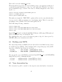
Figure 7: Stokes RR bandshapes of C01 & E05 and W01 & W05;
Figure 8: Stokes LL bandshapes of C03 & C05 E02 & W06 and S04;
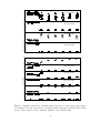
Figure 9: Amplitude and phases of Primary (first scan) and secondary (later
scans) calibrators, (3C286, 1351−018 respectively) on baselines C00 & C01 and
E02, E03 & W06;
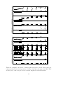
Figure 10: Amplitude and phases of Primary (first scan) and secondary (later
scans) calibrators, (3C286, 1351−018 respectively) on baselines S02, S03 & S06
and W03, W05 & W06.
9000
3500
8000
3000
7000
6000
2500
5000
2000
4000
3000
1500
2000
1000
1000
0
0
20
40
60
80
100
500
120
0
20
40
60
Chan #
350
2000
300
1800
250
1600
200
1400
150
1200
100
1000
50
800
0
0
20
40
60
80
100
120
80
100
120
Chan #
80
100
600
120
Chan #
0
20
40
60
Chan #
Figure 7: Stokes RR bandshapes of C01 & E05 (top two) and W01 & W05 (bottom two),
the spikes seen is an effect of RFIs.
33
1600
4000
1500
3500
1400
3000
1300
2500
1200
2000
1100
1500
1000
1000
900
500
800
0
20
40
60
80
100
0
120
0
20
40
60
Chan #
80
100
120
80
100
120
Chan #
3000
1500
1400
2500
1300
1200
2000
1100
1000
1500
900
800
1000
700
500
0
20
40
60
80
100
600
120
Chan #
0
20
40
60
Chan #
2200
2000
1800
1600
1400
1200
1000
800
600
400
0
20
40
60
80
100
120
Chan #
Figure 8: Stokes LL bandshapes of C03 & C05 (top two), E02 & W06 (middle two) and S04
(bottom one). In S04, the FLAGing (ltaflag) programme has removed the spikes and the
bandshape is fitted with a polynomial.
34
155
150
145
C01-USB-130:C09
140
135
130
125
120
115
110
0.035
105
0.03
C01-USB-130:C09
0.025
0.02
0.015
0.01
0.005
-40
0
-50
C00-USB-130:C09
-60
-70
-80
-90
-100
-110
0.055
-120
0.05
0.045
0.04
0.035
0.03
0.025
0.02
0.015
0.01
0.005
0
C00-USB-130:C09
22
22.5
23
23.5
24
24.5
ist
100
80
60
40
20
0
-20
-40
-60
-80
-100
-120
0.06
E06-USB-130:C09
0.05
E06-USB-130:C09
0.04
0.03
0.02
0.01
2000
150
100
50
0
-50
-100
-150
0.055
-200
0.05
0.045
0.04
0.035
0.03
0.025
0.02
0.015
0.01
0.005
2000
150
100
50
0
-50
-100
-150
-200
0.06
E03-USB-130:C09
E03-USB-130:C09
E02-USB-130:C09
0.05
E02-USB-130:C09
0.04
0.03
0.02
0.01
0
22
22.5
23
23.5
24
24.5
ist
Figure 9: Amplitude and phases of Primary (first scan) and secondary (later scans) calibrators, (3C286, 1351−018 respectively) on baselines C00 & C01 (upper) and E02, E03 & W06
(lower). C09 being the reference antenna, amplitude is in arbitrary units.
35
200
150
100
50
0
-50
-100
-150
-200
0.06
S06-USB-130:C09
0.05
S06-USB-130:C09
0.04
0.03
0.02
0.01
80
0
60
40
20
0
-20
-40
-60
-80
-100
0.055
-120
0.05
0.045
0.04
0.035
0.03
0.025
0.02
0.015
0.01
0.005
2000
150
100
50
0
-50
-100
-150
0.045
-200
0.04
0.035
0.03
0.025
0.02
0.015
0.01
0.005
0
S03-USB-130:C09
S03-USB-130:C09
S02-USB-130:C09
S02-USB-130:C09
22
22.5
23
23.5
24
24.5
ist
200
150
100
50
0
-50
-100
-150
-200
0.04
0.035
0.03
0.025
0.02
0.015
0.01
0.005
2000
150
100
50
0
-50
-100
-150
0.0025
-200
W06-USB-130:C09
W06-USB-130:C09
W05-USB-130:C09
W05-USB-130:C09
0.002
0.0015
0.001
0.0005
2000
150
100
50
0
-50
-100
-150
-200
0.06
W03-USB-130:C09
0.05
W03-USB-130:C09
0.04
0.03
0.02
0.01
0
22
22.5
23
23.5
24
24.5
ist
Figure 10: Amplitude and phases of Primary (first scan) and secondary (later scans) calibrators, (3C286, 1351−018 respectively) on baselines S02, S03 & S06 (upper) and W03, W05
& W06 (lower). C09 being the reference antenna, amplitude is in arbitrary units.
36
. .
37
Part IV
After Observing
6
Your data
Data collected on a particular date are collected into the directory, e.g. ‘/rawdata(1)/date’
(the disk is mounted on mithuna/b is visible from all other PCs). These data are in
LTA format and will have an extension of ‘?.lta(b)’ on the filename. A variety of softwares are available for examining these data in this format. (See GMRT home-page
→ Observing Help → offline data analysis software.).
The most useful for on-site diagnostics is xtract/tax. To run most of this software,
the user must first type, source /astro/RC.csh (or source /astro/RC). The same
software is also available at the NCRA and is sourced in the same way. The programme,
ltacomb is useful to concatenate multiple files and the programme gvfits is required
to convert the data into FITS format for later reading into the Astronomical Image
Processing System (AIPS) of the NRAO.
Spectral line observers who wish to make Doppler corrections can run dopset (again
“source /astro/RC”).
Within AIPS, the user will first have to run INDXR (and it may also be necessary to
run UVSRT). Even for the continuum observations, a bandpass calibration is required,
so the user should proceed with data reductions as for a spectral line data set and
then average the channels later (using SPLAT or SPLIT). Since there is no CHANNEL 0
data set for initial calibration, one possibility (for a sufficiently strong calibrator) is
to first calibrate in time on a single channel and then to apply this calibration when
determining a bandpass solution.
6.1
Interference Monitoring
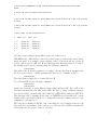
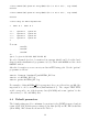
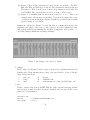
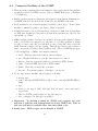
Spectrum analyser in the reciever room shows two kinds of outputs: (1) output from
the optical fibre displaying 130 and 175 MHz channels and (2) the baseband output
displaying the USBs and LSBs. The spectrum analyser output from optical fibre is
shown in the Figure 11.
6.2
Running AIPS at the GMRT
Machines astro1, astro2, astro3, astro4 are generally available for the observers on
priority basis. Please get visitors login and passwd from the local-system-administrator
on these machines (Aniruddha B. Adoni and/or Mangesh Umbarje). You would use
‘/analysis/yourname/’ as your working data area on any one of them. Your data on
mithuna machine (‘/rawdata/6jun/yourfile.lta’) is visible on all other machines at the
GMRT. You also have to ‘source /astro/RC.csh’ or ‘source /astro/RC’, if you wish
to use local packages (e.g. gvfits, tax, etc ...).
39
ACQ STAT : STRTDMP
ACQ STAT : STRTDMP
ANTENNA : C14 TIME : Wed Jul 03 09:57:41 2002
Active Point :
-40.00
ANTENNA : C14 TIME : Wed Jul 03 09:57:41 2002
C02
C14
S06
C10
W01
W02
-50.00
Power (dBm)
-50.00
Power (dBm)
Active Point :
-40.00
-60.00
-70.00
-60.00
-70.00
-80.00
-80.00
-90.00
-90.00
100 110 120 130 140 150 160 170 180 190 200 210
100 110 120 130 140 150 160 170 180 190 200 210
Freq (MHz)
Freq (MHz)
Figure 11: Spectrum analyser output from optical fibre for a few of the antennas, each plot
showing 130 and 175 MHz. S06 (in left Figure) shows spikes (RFIs) in both channels.
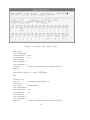
6.3
Primary Beam Gain Correction
Coefficients to use in the task PBCOR in AIPS for primary beam correction of GMRT
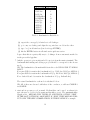
data are tabulated here. The polynomial fit to the beam is 1 + (a/103 )x2 + (b/107 )x4 +
(c/101 0)x6 +(d/101 3)x8 where where x is in terms of (separation from pointing position
in arcmin * frequency in GHz). a,b,c,d are the coefficients which are required to be
specified in PBCOR when using GMRT data. PBPARM(3) (=a), PBPARM(4) (=b),
PBPARM(5) (=c), PBPARM(6) (=d). PBPARM(7)=0 for GMRT. More information
can be found at http://www.ncra.tifr.res.in/∼ngk/primarybeam/beam.html.
Freq band
153 MHz
235 MHz
325 MHz
610 MHz
L band
PBPARM(3)
-4.04
-3.366
-3.397
-3.486
-2.27961
PBPARM(4)
76.2
46.159
47.192
47.749
21.4611
PBPARM(5)
-68.8
-29.963
-30.931
-35.203
-9.7929
PBPARM(6)
22.03
7.529
7.803
10.399
1.80153
Halfpower width
180’
118.5’
85.2’
44.4’
26.2’ ( 1280 MHz)
Table 10: Primary Beam Gain Correction.
6.3.1
Running AIPS on your data
If you are combining data from both the sidebands first run ltamerge to create combined datafile using the following commands :
astro1> ltamerge -i InputLtbFile -I InputLtaFile
40
This would create file ltamerge out.lta.
Then run gvfits (it provides UV data in J2000 epoch); to use gvfits you first need
to run the program listscan to create “log” and “plan” files. Edit the “log” file to
select normalization type, a subset of the data etc. Finally run gvfits on the edited
log file. e.g.
astro1> listscan /rawdata/7jun/01TST01_OBJ.lta
astro1> vi 01TST01_OBJ.log
astro1> gvfits 01TST01_OBJ.log
This makes an output file “TEST.FITS”. gvfits will not work on any files that have
been processed by offline programmes (e.g. ltacleanup, tmac). This is because these
programmes delete elements of the header that gvfits needs.
Start AIPS using following commands :
astro1>
astro1>
astro1>
astro1>
newgrp aips
source /usr/aips/LOGIN.SH (for bash shell)
source /usr/aips/LOGIN.CSH (for csh/tcsh shell)
aips
Begin START AIPS and load this file (01TST01.FITS) into AIPS using FITLD task and
follow your favourite way of reducing the data.
The logflags files can be used as an input in gvfits to flag bad data reported by
ONLINE, while your observations were made.
6.4
Backing your DATA
The data backup facility at GMRT (Section 6.4) includes several 4mm dat tape drives
for 24 GB dat tapes (DDS3). These machines with corresponding tape drive (DATtape-drive or Exabyte tape drive) are as follows:
/dev/nst1
— astro1 machine (4-mm DAT-tape drive)
/dev/nst0
— astro2 machine (4-mm DAT-tape drive)
/dev/rmt/3hn — chitra machine (8-mm Exabyte-tape drive)
Also you can also copy your LTA files (‘/rawdata/7jun/01TST01 .lta’ or ‘01TST01.FITS’)
using DAT-tape-trive on mithuna machine.
/dev/nst0 — mithuna machine (4-mm DAT-tape drive)
/dev/nst1 — mithuna machine (4-mm DAT-tape drive)
6.5
Your observation log
The observation log will be e-mailed to the respective user after his/her observations.
41
6.6
Computer Facilities at the GMRT
• There are many computers placed in terminal room for astronomical data analysis
specificaly reserved for GTAC observer. (also see GMRT Home-page → Facilities
→ Computers)
• Kindly get the relevant account name and password from System Administrator
at GMRT, Khodad. Or check in the Control Room, GMRT for the same.
• In the terminal room, a network printer is available called ’npgcc’. From a linux
machine, command to print is: lpr -Pnpgcc [files] or lpr [files].
• Default data area to get observation files is /rawdata for USB data & /rawdata1
for LSB data. In this area data will be present in the subdirectory called by day
and month e.g. 17may.
• Offline analysis software developed are available. For any path confusion, always
source /etc/bashrc for bash and /etc/csh.cshrc or /etc/cshrc (whichever exists)
for csh (or ’source /astro/RC’ for bash shell or ’source /astro/RC.csh’ for csh/tcsh
shell). Run the sofrware and say explain. This will give help for the software’s
usage. At present following software utilities exist: (also see GMRT home-page
→ Observing Help → Offline data analysis software).
1.
2.
3.
4.
5.
6.
xtract : Extract data from lta file in variuos formats.
tax : Graphical interface to plot the data extracted by ’xtract’.
listscan : List the scan in the ltafile for converting to FITS format.
gvfits : Convert GMRT (lta) data to FITS format.
ltahdr : Gives info about lta file, scan-wise.
ltacomb : Concatenate number of lta files to one lta file.
• To use aips on these machine, after logging do following :
1. newgrp aips
2. source /usr/aips/LOGIN.CSH (for csh) or source /usr/aips/LOGIN.SH (for
bash)
3. aips
4. Prefer to use aips id 1010, 1020 and 1030 on astro1, astro2 and astro3
respectively.
5. There is /DATA partition kept for aips data purpose.
6. Also, /analysis local disk space is available.
• Important : No backup is taken for /DATA and /analysis area and
user has to take his own backup before he leaves GMRT site. Data in
this area will not be available after that more than a day.
• kindly note : DDS-3 tapes can be bought at GMRT.
42
6.7
Computer Facilities at the NCRA
You can use the
(a) computing facilities at the NCRA for your data analysis, please contact V. Venkatasubramani (system administrator) or Shekhar Bachal for accessing visitor (GTAC) machines,
(b) many of the machines in the common computing facility are equipped with either
DAT-tape (DDS3) drive to load and/or back-up your data.
Acknowledgements
This document involves inputs from several people, particularly those associated with
the GMRT. We express our thanks to everyone of them.
Document updated on 4th July 2006 by Manisha Jangam & D.J. Saikia.
43
Appendix Z1. Feedback
Please provide us feedback by filling up the Observer/Visitor Feedback Form available at GMRT home-page.
All publications resulting from the GMRT data should have an acknowledgement of
the form
"We thank the staff of the GMRT who have made these observations
possible. GMRT is run by the National Centre for Radio Astrophysics
of the Tata Institute of Fundamental Research."
44
Appendix Z2. The input files
The source file: The following is the source file, specific example can be picked from
‘/odisk/gtac/source/yourname.list’.
3C286
1637+626
N6503
ISO1
NGC1097
13h28m49.66s
16h37m55.31s
00h40m19.70s
15h36m00.00s
02h46m19.0s
30d45’58.7"
62d40’34.3"
+51d47’07.2"
50d00’00.0"
-30d16’28.0"
1950.0
1950.0
1950.0
2000.0
1950.0
The command file: The following is a simple command file. The consecutive numbers are NOT in the file itself, but are used for the explanation given here. The file
observes a flux density calibrator, 3C286 for 30 minutes first, then a phase calibrator,
1637+626, and then enters a loop in which the phase calibrator and the source, N6503,
are observed consecutively and continuously, with 10 minutes on the phase calibrator
and 30 minutes on-source. In most cases, the first part of the observing session will
not be run from this file but by issuing commands from the monitor, at least until
the user is satisfied that both the flux density calibrator and the first part of a run
on the phase calibrator are satisfactory. Running manually also allows the user to
better determine how much slewing time is required between calibrators and source. If
this is the case, then lines 5 to 23 of this file would be omitted and the resulting file
implemented after the first scan of the phase calibrator is found to be okay. Note that
there is no allowance in this file for a flux density calibration scan in the mid-point
of the observations or at the end. In order to insert such observations, the user must
manually stop this file and issue commands from the console. If the file is restarted,
it will start from the beginning. There is also no end to the file, since the loop, once
entered, has no graceful exit. The session will stop when commands are issued from
the console to stop it. If the array reaches its altitude limit (i.e. the source sets) first,
then it will continue to collect data as instructed in this file while pointing at blank
sky at the array altitude limit (currently 17 degrees).
cmode 1
Specifies that times are relative, rather than absolute.
suba 4
Specifies the subarray being used.
addlist ’/online/operator/source/yourname.list’
Ensures that the system can read the source list.
This must be included in this file, even if already
done manually at the console.
lnkndas
gtsrc ’3c286’
Gets and precesses the coordinates for the specified
source.
goout
Specifies the track (outer or inner) on which slewing
should occur. The choices are goout or goin.
For sources in the northern part of the sky,
45
it’s generally best to use goout.
gosacout
As above, but required for the subarray controller.
The choices are gosacout and gosacin.
sndsacsrc(1,12h) Slew to the source and start tracking (1)
for up to 5 hours (5h).
time 5m
Do not do anything for 5 minutes in order to allow the
array to reach its target.
strtndasc
Start the correlator and collect data.
time 10m
Continue to collect data for 10 minutes.
hold; stabct
Release the brakes (hold) in case minor wind gusts
have resulted in the brakes being applied automatically
at some point during the observations. For
strong winds, an alarm will sound in the control
room. And set the time at the antenna based computer
(stabct).
time 10m
Keep collecting data for another 10 minutes.
stpndasc
Stop the correlator (i.e. stop collecting data).
stpsactrk
Stop tracking.
gtsrc ’1637+626’ Get and precess coordinates for the second source,
here the phase calibrator.
goout
gosacout
sndsacsrc(1,5h)
time 6m
$1
starts the loop
gtsrc ’1637+626’
goout
gosacout
sndsacsrc(1,12h)
time 2m &
strtndasc
time 10m
stpndascan
stpsactrk
gtsrc ’N6503’
goout
gosacout
sndsacsrc(1,5h)
time 2m
strtndasc
time 10m
hold;stabct
time 10m
46
hold;stabct
time 10m
hold;stabct
stpndascan
go to 1
returns to the beginning of the loop.
end
---------------------------------------------------------------------------A few examples of command files are shown below (each column is an independent
command file):
47
cmode 1
cmode 1
addlist ’/temp2/data/source/01TST1.list’ addlist ’/temp2/data/source/01TST1.list’
addlist ’/temp2/data/source/01TST1.list’ lnkndas
lnkndas
suba 4
suba 4
goout
goin
gosacout
gosacin
cp 0
cp 0
gts ’3C286’
gts ’0237−23’
sndsacsrc(1,1h)
sndsacsrc(1,1h)
time 0.2m
time 0.5m
sndsacsrc(1,1h)
sndsacsrc(1,1h)
stabct
stabct
strtndasc
strtndasc
time 10.0m
time 10.0m
stpndasc
stpndasc
gts ’1323+32’
gts ’0213−132’
sndsacsrc(1,1h)
sndsacsrc(1,1h)
time 1.0m
time 1.5m
sndsacsrc(1,1h)
sndsacsrc(1,1h)
stabct
stabct
strtndasc
strtndasc
time 10.0m
time 10.0m
stpndasc
stpndasc
gts ’1328+25’
gts ’0235−19’
sndsacsrc(1,1h)
sndsacsrc(1,1h)
time 1.0m
time 1.0m
sndsacsrc(1,1h)
sndsacsrc(1,1h)
stabct
stabct
strtndasc
strtndasc
time 10.0m
time 10.0m
stpndasc
stpndasc
gts ’1350+31’
gts ’0240−00’
sndsacsrc(1,1h)
sndsacsrc(1,1h)
time 1.0m
time 1.0m
sndsacsrc(1,1h)
sndsacsrc(1,1h)
stabct
stabct
strtndasc
strtndasc
time 10.0m
time 10.0m
stpndasc
stpndasc
gts ’3C286’
gts ’0349−27’
sndsacsrc(1,1h)
sndsacsrc(1,1h)
time 1.0m
time 1.0m
sndsacsrc(1,1h)
sndsacsrc(1,1h)
stabct
time 1.0m
strtndasc
sndsacsrc(1,1h)
time 10.0m
stabct
stpndasc
strtndasc
time 10.0m
end
stpndasc
gts ’0403−13’
sndsacsrc(1,1h)
time 1.0m
sndsacsrc(1,1h)
stabct
strtndasc
time 10.0m
stpndasc
gts ’0442−28’
sndsacsrc(1,1h)
time 1.0m
sndsacsrc(1,1h)
stabct
strtndasc
time 10.0m
stpndasc
end
48
cmode 1
lnkndas
subar 4
goout
gosacout
cmode 1
dellist 2
addlist ’/temp2/data/source/01TST1.list’
lnkndasq
subar 4
goout
gosacout
addlist ’/temp2/data/source/vlacal.list’
addlist ’/temp2/data/source/01TST1.list’ $1
$1
gts ’2139+143’
sndsacsrc(1,1h)
time 0.5m
sndsacsrc(1,1h)
stabct
strtndasc
time 5.0m
stpndasc
gts ’2232+117’
sndsacsrc(1,1h)
time 0.5m
sndsacsrc(1,1h)
stabct
strtndasc
time 5.0m
stpndasc
gts ’3C433’
sndsacsrc(1,1h)
time 0.5m
sndsacsrc(1,1h)
stabct
strtndasc
time 8m
hold;stabct
time 8m
hold;stabct
time 8m
hold;stabct
time 8m
stpndasc
goto 1
end
stpsactrk
gts ’1035+564’
sndsacsrc (1,1h)
time 1m
sndsacsrc (1,1h)
stabct
strtndasc
time 10m
stpndasc
stpsactrk
gts ’1116+517’
sndsacsrc (1,1h)
time 1m
sndsacsrc (1,1h)
stabct
strtndasc
time 10m
hold;stabct
time 10m
hold;stabct
time 10m
hold;stabct
stpndasc
goto 1
end
Appendix Z3. The trouble-shooting
The trouble-shooting
1. Fringes Disappeared ?
(a) stpdasc; gts ‘srcname’; strtdasc
(b) are antennas tracking your source ? have they hit the azimuth limit ?
(c) is your source extended ?
(d) has any of correlator software crashed ?
(e) have the front-end parameters got reset ? ask the observer.
2. Fringes are winding ?
(a) check LO 1 and LO 4 settings.
(b) stpdasc; tparm, prjfreq, gts ’srcname’; strtndas
(c) check time synchronisation between correlator PCs and ONLINE PC and
GPS time.
(d) ionospheric variations ? The winding will be random.
3. Fstop window says ’link reset; packet transmission not possible’
(a) fstop has crashed.
4. Some baselines record low cross-correlation on a point source ?
(a) Is polarisation swap, required on some antennas, applied ?
(b) Are the self-correlations of problem antennas as expected ?
(c) Are pointing offsets being loaded ?
(d) stpdasc; gts ‘srcname’; strtdasc
5. The LTA and AIPS file header shows RF=0 Hz, IF LO=0 Hz, BB LO=0 Hz ?
(a) If noticed during observations, stpdasc and stpdass and start again. Don’t
forget to set TPARM (Frequency parameters to correlator).
(b) If noticed after observations, forget about that data and get a fresh run.
49