1
ReaxFF User Manual
Written by Adri van Duin, December 2002
E-mail: [email protected]
Materials and Process Simulation Center
Beckman Institute (139-74)
California Institute of Technology
Pasadena, CA 91125
USA
1
Contents
1. General overview
1.1. Concept
1.2. Features
1.3. Performance
1.4. Current force fields
2. Input files
2.1. General remarks
2.2. Mandatory input files
2.3. Optional input files
2.4. Force field optimization input files
3. Output files
3.1. General remarks
3.2. MM and MD output files
3.3. Force field optimization output files
4. Potential functions
5. Program structure
6. Literature
2
1. General overview
1.1 Concept. ReaxFF was developed to bridge the gap between quantum chemical
(QC) and empirical force field (EFF) based computational chemical methods (Figure
1.1). Where QC methods are, in general, applicable to all chemical systems, regardless of
connectivity, their computational expense makes them inapplicable for large (say, more
than100 atoms) systems. Their computational expense also makes QC methods primarily
applicable for single point or local energy minimization; high-temperature molecular
dynamics (MD) simulations are generally too time-consuming.
Hierarchy of computational chemical methods
MD
QC
10-15
Design
FEA
Time
years
Atoms
Molecular
Electrons conformations
Bond formation
MESO
Ångstrom
QC methods:
- Allow reactions
- Expensive, only
small systems
Simulate bond formation
in larger molecular systems
ReaxFF
ab initio,
DFT,
HF
Empirical methods:
- Allow large systems
- Rigid connectivity
Empirical
force fields
Distance
Kilometres
Figure 1.1: Position of ReaxFF in the computational chemical hierarchy.
EFF methods describe the relationship between energy and geometry with a set of
relatively simple potential functions. In their most simple form, EFF methods describe
molecular or condensed phase systems by simple harmonic equations that describe the
stretching and compression of bonds and the bending of bond angles, usually augmented
by van der Waals potential functions and Coulomb interactions to describe non-bonded
interactions. Their relative simplicity allows EFF methods to be applied to much larger
systems than QC systems (thousands of atoms on single processors; millions of atoms on
multiprocessors). EFF methods have been very successful in describing physical
interactions in and between molecules and condensed phase systems, and EFF methods
haven been developed for a wide variety of chemical environments, including
hydrocarbons [lit], proteins [lit] and many inorganic systems [lit]. However, EFF
methods are mainly applicable for systems at or around their equilibrium configuration.
Due to their empirical nature, EFF methods require that the parameters used in their
3
potential functions are fitted against a suite of data, which can be gathered from
experimental and/or from QC-sources (a.k.a. training set). The force field resulting from
this fitting procedure can obviously be no more reliable than the data used in its training
set. Furthermore, as the force field describes the system in an empirical rather than
fundamental fashion, it should only be applied to systems similar to the ones present in
the training set. As such, the quality and diversity of the training set define the
transferability of the EFF method. With a few exceptions, current EFF methods are only
trained for systems in which the bonds remain within about 75% of their equilibrium
value. For this reason, these EFF methods cannot describe reactive systems, and in most
cases the shape of the potential functions applied in these methods, like the
aforementioned harmonic description of the bond length/bond energy relationship, would
make it impossible to find parameter values that accurately describe bond energy towards
the dissociation limit.
The concept of bond order/bond energy relation, as first formulated by Tersoff [lit],
allows for the construction of EFF methods that can, in principle, handle connectivity
changes. This concept was used by Brenner [lit] to construct the REBO-potential, an EFF
method for hydrocarbon systems, allowing, for the first time, dynamical simulations of
reactions in large (>>100 atoms) systems. Over the years, REBO has enjoyed widespread
application, but its transferability is limited as it is based on a relatively small training set
and because of its exclusion of all non-bonded interactions.
As with the Brenner potential, a bond order/bond energy relationship lies at the center
of the ReaxFF-potential. Bond orders are obtained from interatomic distances (Figure 2)
and are continually updated at every MD or energy minimization (MM) iteration, thus
allowing for connectivity changes. These bond orders are incorporated in all valence
terms (i.e. energy contributions dependent on connectivity, like valence angle and torsion
angle energy) ensuring that energies and forces associated with these terms go to zero
upon dissociation. Furthermore, ReaxFF describes non-bonded interactions between all
atoms, irrespective of connectivity. Excessive short-range repulsive/attractive nonbonded interactions are circumvented by inclusion of a shielding term in the van der
Waals and Coulomb interaction. For a more detailed description of the ReaxFF energy
description see [lit].
ReaxFF aims to provide a transferable potential, applicable to a wide range of
chemical environments. To ensure its transferability, the following general guidelines
have been adopted in its development:
- No discontinuities in energy or forces, even during reactions.
- Each element is described by just one force field atom type. The ReaxFF metal
oxide oxygen is described by the same parameters as the ReaxFF oxygen in organic
molecules. ReaxFF does not have separate sp2 and sp3 atoms for carbon, the method
determines the atoms hybridization from its chemical environment.
- No pre-definition of reactive sites is necessary using ReaxFF. Although it is
possible to drive reactions using restraints (see Input files section) this is not required;
given the right temperature and chemical environment reactions will happen
automatically.
1.2 Features. At the moment of writing this manual, the ReaxFF-program supports
the following features:
4
- NVT and NVE dynamics; limited NPT dynamics for molecular systems. Velocity
and system volume scaling are performed using the Berendsen method [ref]. Velocity
scaling can be performed on the entire system, on individual molecules or on individual
atoms. Different temperature regimes can be applied to different parts of the system using
the tregime.in file. This input file can also be used to increase and decrease system
temperature during an MD-simulation and can be used to set op annealing runs.
- Steepest descent and conjugate gradient minimization methods.
- Numerical optimization of cell parameters. Default setting is for cubic
optimization, but a/b/c parameters can be optimized separately. Also, c/a ratios can be
varied separately (see sections on control and input geometry files).
- ReaxFF supports interatomic distance, angle, torsion angle and centre-of-mass
restraints. These restraints can be used to drive reactions and can be defined in the geofile (in .bgf-format). Sliding interatomic distance, angle and torsion restraints can be used
in MD-simulations.
- ReaxFF can perform simulations on crystal unit cells, keeping track of bonds and
valence angles between periodic images of atoms. Currently, this feature cannot be
applied to systems requiring torsion angles across periodic boundaries (e.g. carbon
crystals). None of the inorganic ReaxFF force fields developed to date have included
torsion energy terms, and as such ReaxFF can do unit cell calculations for these systems.
ReaxFF can also be used to create supercell structures (fort.86-output file).
- ReaxFF contains a force field optimization module. See input and output file
sections for a further description.
- ReaxFF has been developed around the EEM charge derivation method [ref],
allowing calculation of geometry dependent charge distributions. As default, ReaxFF
equilibrates the charges over the entire systems, however, it can also equilibrate charges
within each molecule or run with fixed charges (see control-file and charges-file in the
input file section).
- ReaxFF generates. bgf, .geo, .xyz, .MOP, z-matrix (for molecules) and .pdf output
files and can read .geo, .bgf, .xyz and z-matrix files. Trajectories are saved in .xyzformat, with optional velocities. Restart files are generated at user-specified intervals.
1.3 Performance. Calculation speed for ReaxFF greatly depends on the atom
connectivity. Slowest calculation speed is obtained for high-density crystal systems
requiring valence angle and torsion potentials (i.e. diamond). Table 1.1 shows the
ReaxFF calculation speed for some benchmark systems. To date, the largest system
ReaxFF has been applied for contained about 5000 atoms. Future developments in
parallelizing the ReaxFF-code should greatly increase the feasible system size.
At low and medium temperatures (0-1500K) ReaxFF can run with time-steps of up to
0.5 femtoseconds and retain reasonable energy conservation. At higher temperatures
smaller time-steps are required to retain energy conservation.
5
Table 1.1: Benchmark runs for some crystal and molecular systems. Simulations
were performed on a single-processor Compaq XP1000-workstation. The Diamond
crystal calculations involved valence and torsion angle energies, the Si(a)
calculations did only involve valence angle energies.
System
#atoms
Time/MD simulation (s)
Diamond crystal (r=??)
64
0.5
Diamond crystal (r=??)
256
4
Si(a) crystal (r=??)
64
0.25
Si(a) crystal (r=??)
256
2
13 Methane molecules (r=??)
65
0.1
52 Methane molecules (r=??)
260
0.4
1.4 Current force fields. Table 1.2 shows for which systems ReaxFF has currently
been parameterized and at which stage of development these parameters sets are. Note
that there often exists a substantial overlap between the parameter sets mentioned in
Table 1.2. for example, the ReaxFFRDX parameter set contains the same carbon/hydrogen
parameters as ReaxFFCH, while the various metal oxide reactive force fields all share the
same oxygen parameters, in accordance with the aforementioned ReaxFF philosophy of
transferability.
Table 1.2: Currently available ReaxFF parameter set with quality denomination. *
means that parameterization has only been performed for against a fairly limited training
set, ** indicates that the parameters have been tested against a reasonably good training
set but that further modifications and improvements are expected, *** indicates that
these parameters have reached the application-stage.
Name
System
Quality
Reference
ReaxFFCH
Hydrocarbons
***
[lit,lit]
CH
ReaxFF
All-carbon (buckyballs, nanotubes)
**
ReaxFFRDX
Nitramines
***
[lit]
CONSH
ReaxFF
CONSH-systems, proteins
**
ReaxFFSiO
Si/SiO2 clusters and condensed phase
***
[lit]
AlO
ReaxFF
Al/AlO
***
ReaxFFSiN
SiN clusters and condensed phase
*
ZrO
ReaxFF
Zr and ZrO2 condensed phase
*
ReaxFFMoO
Mo and Mo-oxides
**
Pt
ReaxFF
Pt bulk metal; Pt-C, Pt-H and Pt-O systems *
-
Training sets for these force fields primarily, and for many systems exclusively,
consist of QC data on clusters and condensed phases. Although some of these reactive
potentials have been applied successfully neither of these parameter sets are considered
final. Our approach is that during an application we will continuously scrutinize the
ReaxFF results by checking against QC data (probably by performing targeted QCsimulations on representative small systems). When major discrepancies occur the QC
data can be added to the appropriate training set and the parameters can be re-optimized.
6
By this continuous communication between QC and ReaxFF we should obtain
increasingly reliable and transferable reactive force field descriptions.
7
2. Input Files
2.1 General. The ReaxFF input files can be divided into mandatory files, which are
necessary for the program to run, and optional files, which are only needed for specific
applications. Table 2.1 gives an overview of the input files.
Table 2.1: Overview of ReaxFF input files.
File name
Section
geo
Mandatory
ffield
Mandatory
control
Mandatory
exe
Mandatory
models.in
Optional
tregime.in
Optional
iopt
Optional
charges
vels
trainset.in
params
Optional
Optional
Force field optimization
Force field optimization
koppel2
Force field optimization
Short description
system geometry
force field parameters
run control switches
executable script
geometry file location
temperature regime
definition
normal run/force field
optimization toggle
fixed charges
restart-file
training set definition
optimizable force field
parameters
links values force field
parameters
2.2 Mandatory files.
geo-file. This file describes the system geometry. Currently, ReaxFF supports the
.geo, .bgf, .xyz and z-matrix input formats (see examples below). By default, ReaxFF
assumes geo contains a .geo or a z-matrix format; to use other formats the igeofor-switch
in the control-file should be given a value of 1 for .bgf format and a value of 2 for .xyzformat. Future developments will be primarily centered around the .bgf-format and will
move away from the .geo-format. As such, only a brief description of the .geo-format will
be given in this manual.
All geo-input formats are format sensitive. Below follows a discussion of several
examples of geo-input files.
8
Example 2.1: Non-periodic .bgf-input file.
BIOGRF 200
DESCRP Ethane_radical.
REMARK Example
RUTYPE NORMAL RUN
# THIS LINE IS IGNORED
FORMAT ATOM (a6,1x,i5,1x,a5,1x,a3,1x,a1,1x,a5,3f10.5,1x,a5,i3,i2,1x,f8.5)
HETATM 1 C
39.53649 39.80304 39.57992 C 1 1 -0.2894
HETATM 2 H
39.96404 38.93497 39.07954 H 1 1 0.1031
HETATM 3 C
40.55862 40.34907 40.60075 C 1 1 -0.2330
HETATM 4 H
39.30695 40.55630 38.82721 H 1 1 0.1048
HETATM 5 H
38.62048 39.49467 40.08241 H 1 1 0.1048
HETATM 6 H
40.65314 39.88418 41.56157 H 1 1 0.1048
HETATM 7 H
41.36027 40.97776 40.26860 H 1 1 0.1048
FORMAT CONECT (a6,12i6)
CONECT 1 2 3 4 5
CONECT 2 1
CONECT 3 1 6 7
CONECT 4 1
CONECT 5 1
CONECT 6 3
CONECT 7 3
END
Example 2.1 shows a basic, non-periodic .bgf-input file. .bgf is a keyword-driven
input format; each line starts with a keyword followed by information associated with
that keyword. The .bgf-format is used by various molecular simulation software packages
(i.e. Cerius2, Jaguar). As these programs should ignore lines starting with unrecognized
keywords the .bgf-format should be easily portable between different applications.
ReaxFF recognizes the following .bgf-keywords:
B IOGRF [VERSION NUMBER]: defines .bgf-version number. ReaxFF reads
version number 200 (and will stop if other version numbers are provided).
DESCRP [NAME]: System description. This description can be used in trainset.in to
define a force field training set.
REMARK: Remarks. Multiple REMARK lines are allowed.
RUTYPE [KEYWORD ;NUMBER]: Defines run parameters. If KEYWORD is
NORMAL RUN (as in Example 2.1) ReaxFF uses the switches defined in the controlfile. Alternatively, switches in the control-file can be overridden by the KEYWORD
options listed in Table 2.2. This options is useful in force field optimizations as different
MM-methods can be used for different training set geometries. If no RUTYPE-line is
supplied, ReaxFF uses the control-file definitions
9
Table 2.2: RUTYPE keywords supported by ReaxFF.
KEYWORD
Description
NORMAL RUN
Use switches in control-file
MAXIT [NUMBER]
Stop MM-run after NUMBER iterations
ENDPO [NUMBER]
Stop MM-run when RMSG drops below NUMBER
MAXMOV [NUMBER] Maximum atom movement (in 10-6 Å) during steepest
descent MM minimization. With NUMBER=0 a conjugate
gradient method is used.
SINGLE POINT
Stop MM-run after first point
DOUBLE PRECISION
Double MM maximum number of iterations and half
RMSG end point criterion as defined in control-file
LOW PRECISION
Half MM maximum number of iterations as defined in
control-file
CELL OPT [NUMBER] Perform numerical cell optimization in MM. See controlfile for options defined by NUMBER
NO CELL OPT
Do not perform numerical cell optimization
FORMAT [STRING]: Supplies format-information. ReaxFF ignores these FORMAT
lines; they cannot be used to modify input formatting.
HETATM [ATOM INFO]: Defines atom type and atom position. In this order, the
ATOM INFO consists of the atom number, the atom type, the x, y and z-coordinates of
the atom in Å, the force field type (same as atom type for ReaxFF), two switches not used
by ReaxFF and the atom partial charge. ReaxFF does not use these partial charges.
CONECT [ATOM NUMBER:CONNECTED ATOM NUMBERS]: Connection
table. ReaxFF ignores these lines and calculates its own connections.
END: Last line of .bgf-input geometry.
Line starting with a # are ignored by ReaxFF and can be used to supply additional
comment.
Example 2.2: Periodic .bgf-input geometry file.
XTLGRF 200
DESCRP fcc_1
REMARK Platinum fcc-structure
RUTYPE NORMAL RUN
CRYSTX 4.50640 4.50640 4.50640 90.00000 90.00000 90.00000
FORMAT ATOM (a6,1x,i5,1x,a5,1x,a3,1x,a1,1x,a5,3f10.5,1x,a5,i3,i2,1x,f8.5)
HETATM 1 Pt
0.00000 0.00000 0.00000 Pt 1 1 0.00000
HETATM 2 Pt
2.25138 2.25138 0.00000 Pt 1 1 0.00000
HETATM 3 Pt
2.25138 0.00000 2.25138 Pt 1 1 0.00000
HETATM 4 Pt
0.00000 2.25138 2.25138 Pt 1 1 0.00000
FORMAT CONECT (a6,12i6)
END
10
Example 2.2 shows a periodic .bgf-input file. In principle, ReaxFF treats every
system as periodic; in non-periodic systems it simply uses large values for the cell
parameters (these values are defined by the axis1, axis2 and axis3-switches in the
control-file). However, these control-file definitions are ignored if cell parameters are
defined in the geo-file. Example 2.2 features the following keywords in addition to
Example 2.1:
XTLGRF [VERSION NUMBER]: As BIOGRF-keyword, but tells ReaxFF that userspecified cell parameters are supplied with this geometry.
CRYSTX [A B C Alpha Beta Gamma]: Defines cell lengths (in Å) and cell angles
(in degrees) for periodic system.
ReaxFF always uses Cartesian (not fractional) coordinates to define atom positions.
The .bgf-input format can also be used to define interatomic, valence angle, torsion
angle and center-of-mass restraints used during MM or MD simulations. Such restraints
can be used to drive reactions or to force conformational changes. Example 2.3 shows the
Example 2.3: .bgf-input file with restraints.
BIOGRF 200
DESCRP Hshift11
RUTYPE NORMAL RUN
FORMAT BOND RESTRAINT (15x,2i4,f8.4,f8.2,f8.5,f10.7)
#
At1 At2 R12 Force1 Force2 dR12/dIteration(MD only)
BOND RESTRAINT 1 2 1.0900 7500.00 0.25000 0.0000000
FORMAT ANGLE RESTRAINT (16x,3i4,2f8.2,f8.4,f9.6)
#
At1 At2 At3 Angle Force1 Force2 dAngle/dIteration
(MD)
ANGLE RESTRAINT 1 2 3 120.00 250.00 1.00000 0.0000
FORMAT TORSION RESTRAINT (18x,4i4,2f8.2,f8.4,f9.6)
#
At1 At2 At3 At4 Angle Force1 Force2 dAngle/dIt
TORSION RESTRAINT 1 2 3 4 45.00 250.00 1.00000 0.0000
FORMAT MASCEN RESTRAINT FREE FORMAT
#
x/y/z At1 At2 R At3 At4 Force1 Force2
MASCEN RESTRAINT x 1 3 1.50 4 7 50.00 0.25
FORMAT ATOM (a6,1x,i5,1x,a5,1x,a3,1x,a1,1x,a5,3f10.5,1x,a5,i3,i2,1x,f8.5)
HETATM 1 C
39.53692 39.80281 39.57996 C 1 1 0.00000
HETATM 2 H
39.96200 38.93424 39.07781 H 1 1 0.00000
HETATM 3 C
40.55717 40.34771 40.59881 C 1 1 0.00000
HETATM 4 H
39.30845 40.55556 38.82947 H 1 1 0.00000
HETATM 5 H
38.62310 39.49566 40.08262 H 1 1 0.00000
HETATM 6 H
40.65332 39.88631 41.56086 H 1 1 0.00000
HETATM 7 H
41.35903 40.97771 40.27048 H 1 1 0.00000
FORMAT CONECT (a6,12i6)
END
11
available restraint input options. The FORMAT lines give the required input format for
these restraints. Example 2.3 features the following keywords:
BOND RESTRAINT [At1 At2 R12 Force1 Force2 dR12/dIteration]: Defines bond
(i.e. interatomic) restraint between atoms At1 and At2. An additional force is added to the
ReaxFF potential, aiming to keep the distance between At1 and At2 restraint at value
R12. Force1 and Force2 are the force constants used for this additional force, which is
defined in Equation 2.1:
Erestraint= Force1*{1.0-exp(Force2*(Rij-R12)2}
Equation 2.1
During MD-simulations the value of R12 will be modified by dR12/dIteration every
iteration. By using this feature, ReaxFF can drive reactions during MD simulations. This
option is not available during MM minimizations.
ANGLE RESTRAINT [At1 At2 At3 Angle Force1 Force2 dAngle/dIteration]:
Defines angle restraint between atoms At1, At2 and At3. Any angle in the system can be
restrained in this way, independent of connectivity. An additional force, similar to
Equation 2.1, is added to the ReaxFF potential. As with the bond restraint,
dAngle/dIteration can be used to drive angles during an MD simulation.
TORSION RESTRAINT [At1 At2 At3 At4 Angle Force1 Force2 dAngle/dIteration]:
Defines torsion angle restraint between atoms At1, At2, At3 and At4. At this moment,
this restraint can ONLY be used between connected atoms. In defining the torsion angle
At2 should be smaller than At3. Force1 and Force2 define an additional force, similar to
that described by Equation 1.2, that is added to the ReaxFF potential. dAngle/dIteration
can be used to drive torsion angles during an MD simulation. Driving a torsion angle
through 0º or through 180 º might cause problems.
MASCEN RESTRAINT [x/y/z At1 At2 R At3 At4 Force1 Force2]: Defines centerof-mass restraints between atoms At1 to At2 and atoms At3 to At4 in either the x, y or zdirection. An additional force, similar to that described in Equation 2.1, is added to the
ReaxFF potential, restraining the center-of-mass of atoms At1 to At2 at distance R in the
x/y/z directions from the center-of-mass of atoms At3 to At4.
To facilitate building training sets with multiple geometries, ReaxFF can run multiple
simulations from one geo-file. This is done by putting these geometries in one geo-file,
separated by one empty line after each END-keyword. Alternatively, the models.in-file
can be used to define the paths to these multiple geo-files.
When combining multiple geometries in one geo-file, ReaxFF can repeat simulations
on the previous input geometry with modified cell volume. This is useful for obtaining
equation of state information for condensed phase systems. Example 2.4 shows an .bgfinput file from which ReaxFF first runs a single point simulation on a Pt-fcc unit cell,
followed by a simulation on the same structure in which the cell volume is reduced by
80% (and the atomic positions are rescaled accordingly). This is done using the
VCHANGE keyword:
VCHANGE [NUMBER]: repeat the previous simulation with rescaled cell volume
and atomic coordinates. The rescaling factor is NUMBER*100%. ReaxFF will
automatically use the RUTYPE NO CELL OPT (Table 2.2) option for structure specified
with VCHANGE.
12
As mentioned, future ReaxFF input file developments will primarily focus around the
.bgf-format. Anticipated developments include:
- Making the .bgf-input format free.
- Making more control-file options available through .bgf-file input, thus allowing
all run-input information to be supplied in only one input file.
- Allowing addition of force field training set information (charges, energies) to the
.bgf-file. This information should be automatically picked up by ReaxFF and compared
to ReaxFF output.
Example 2.4: Periodic .bgf-input geometry file followed by VCHANGE option.
XTLGRF 200
DESCRP fcc_1
REMARK Platinum fcc-structure
RUTYPE SINGLE POINT
CRYSTX 4.50640 4.50640 4.50640 90.00000 90.00000 90.00000
FORMAT ATOM (a6,1x,i5,1x,a5,1x,a3,1x,a1,1x,a5,3f10.5,1x,a5,i3,i2,1x,f8.5)
HETATM 1 Pt
0.00000 0.00000 0.00000 Pt 1 1 0.00000
HETATM 2 Pt
2.25138 2.25138 0.00000 Pt 1 1 0.00000
HETATM 3 Pt
2.25138 0.00000 2.25138 Pt 1 1 0.00000
HETATM 4 Pt
0.00000 2.25138 2.25138 Pt 1 1 0.00000
FORMAT CONECT (a6,12i6)
END
XTLGRF 200
DESCRP fcc_2
REMARK Rerun fcc_1 at 80% volume
VCHANGE 0.80
END
As an alternative to the .bgf-input format, ReaxFF can also read .geo-, .xyz- and zmatrix formats. Example 2.5 shows an ReaxFF .geo input file. The first line of the .geoformat contains a control-character (C in Example 2.5) and the name of the structure. The
next lines contain the atom number, atom type and the x,y and z-coordinates. By means
of the control-character, the .geo-format provides most of the options available with the
.bgf-format. As we are moving away from supporting the .geo-format we only summarize
these options in Table 2.3; more information can be obtained from the author.
13
Example 2.5: .geo-input file.
C Ethyl_radical
1C
2H
3C
4H
5H
6H
7H
0.39536921883140E+02
0.39962000508882E+02
0.40557168455097E+02
0.39308447421804E+02
0.38623101361336E+02
0.40653318128573E+02
0.41359032241168E+02
0.39802812097390E+02
0.38934237894502E+02
0.40347711311539E+02
0.40555557250666E+02
0.39495660102816E+02
0.39886313307789E+02
0.40977708035298E+02
0.39579964797377E+02
0.39077807973956E+02
0.40598809008712E+02
0.38829468433362E+02
0.40082615760111E+02
0.41560863579234E+02
0.40270480449231E+02
Table 2.3 Control character options available with .geo-format.
Control character
Effect
C
Normal run as defined in control-file
F
Use cell parameters (defined on lines 2+3 of .geo-format)
1
Single point
D
Double precision run
H
Low precision run
5
Use cell parameters; single point
Example 2.6: z-matrix input file.
I
2
2
5
5
Ethyl_radical
1 C
1 2 C
1 2 3 C
3 1 4 H -119.14400
3 1 5 H 119.14417
1 3 6 H
38.20847
1 3 7 H -159.92026
42.38253
110.52474
110.52466
120.04903
120.04917
1.08962
2.15999
1.08723
1.08723
1.07130
1.07130
Example 2.6 demonstrates the ReaxFF z-matrix input format. The ‘I’ on position 3 on
the first line is required as a format-type identifier and is followed by the structure name.
The following lines have the 4i3,1x,a2,3f10.5 format and contain atl, atk, atj, ati, atype,
torsijkl, angleijk and Rij, where torsijkl is the ati-atj-atk-atl torsion angle, angleijk the ati-atj-atk
angle, Rij the ati-atj interatomic distance and atype the atom type of ati. By using internal
instead of Cartesian coordinates, the z-matrix-input format facilitates building molecules.
The z-matrix does not provide room to define cell parameters and, as such, can only be
used in concert with the default cell parameters axis1, axis2 and axis3 from the controlfile.
14
Example 2.7: .xyz-input file.
7
Ethyl_radical
C 39.53692 39.80281
H 39.96200 38.93424
C 40.55717 40.34771
H 39.30845 40.55556
H 38.62310 39.49566
H 40.65332 39.88631
H 41.35903 40.97771
39.57996
39.07781
40.59881
38.82947
40.08262
41.56086
40.27048
ReaxFF supports the .xyz-format in Example 2.7 because its simplicity facilitates
communication with other simulation software and molecular viewers (e.g Icarus,
Molden and Xmol). The first line of the .xyz-format contains the number of atoms, the
second line the structure name. The other lines contain the type and x,y,z Cartesian
coordinates for each of the atoms. The .xyz format cannot communicate cell parameters
and, as such, can only be used with the default cell parameters axis1, axis2 and axis3
defined in the control-file.
ffield-file. The ffield input file contains the force field parameters. The first line of
the ffield-input file contains a force field identifier (Example 2.8). Thereafter, the force
field is divided into 7 sections, containing the general, atom, bond, off-diagonal, valence
angle, torsion angle and hydrogen bond parameters. Below follows a description of the
format and meaning of the force field parameters in each of these sections.
15
Example 2.8: ffield-input file.
Force field identifier
Reactive MD-force field: Hydrocarbon parameters
39
! Number of general parameters
50.0000 !Overcoordination parameter
9.8407 !Overcoordination parameter
21.2839 !Valency angle conjugation parameter
3.0000 !Triple bond stabilisation parameter
6.5000 !Triple bond stabilisation parameter
1.0000 !Not used
0.9782 !Undercoordination parameter
1.0250 !Triple bond stabilisation parameter
General
6.3452 !Undercoordination parameter
11.6274 !Undercoordination parameter
0.0000 !Triple bond stabilization energy
0.0000 !Lower Taper-radius
10.0000 !Upper Taper-radius
2.8793 !Not used
33.8667 !Valency undercoordination
88.6186 !Valency angle/lone pair parameter
1.0563 !Valency angle
2.0384 !Valency angle parameter
6.1431 !Not used
7.5203 !Double bond/angle parameter
0.3989 !Double bond/angle parameter: overcoord
3.9954 !Double bond/angle parameter: overcoord
-2.4837 !Not used
4.7120 !Torsion/BO parameter
10.0000 !Torsion overcoordination
2.3170 !Torsion overcoordination
-1.2635 !Conjugation 0 (not used)
2.1645 !Conjugation
1.4553 !vdWaals shielding
0.1000 !Cutoff for bond order (*100)
2.8921 !Valency angle conjugation parameter
7.1783 !Overcoordination parameter
1.4473 !Overcoordination parameter
3.1353 !Valency/lone pair parameter
0.5000 !Not used
Parameter identifiers
20.0000 !Not used
5.0000 !Molecular energy (not used)
0.0000 !Molecular energy (not used)
1.6052 !Valency angle conjugation parameter
2
cov.r; valency; a.m;
Rvdw;
Evdw;
gammaEEM; cov.r2; #el
alfa; gammavdW; valency; Eunder; n.u.;
chiEEM;
etaEEM; n.u.
cov r3;Elp;
Heat inc.;13BO1; 13BO2; 13BO3;
n.u.;
n.u.
ov/un; val1;
n.u.;
val3; vval4; n.u.;
n.u.;
n.u.
C
1.3826
4.0000 12.0000
2.0195
0.0763
0.8712
1.2360
4.0000
10.6359
1.9232
4.0000 40.5154
0.0000
5.7254
6.9235
0.0000
Atom
1.1663
0.0000 200.0498
6.1551 28.6991 12.1086
0.0000
0.0000
-14.1953
3.5288
0.0000
6.2998
2.9663
0.0000
0.0000
0.0000
H
0.6510
1.0000
1.0080
1.7693
0.0244
0.7625 -0.1000
1.0000
10.0482
5.2587
1.0000
0.0000
0.0000
3.8196
9.8832
1.0000
-0.1000
0.0000 65.0500
3.7647
2.7644
1.0000
0.0000
0.0000
-13.3669
3.6915
0.0000
6.2998
2.8793
0.0000
0.0000
0.0000
3
Edis1;
Edis2;
Edis3;
pbe1;
pbo5;
13corr; pbo6;
kov
pbe2;
pbo3;
pbo4;
n.u.;
pbo1;
pbo2;
ovcorr;
n.u.
1 1 152.0140 104.0507 72.1693
0.2447 -0.7132
1.0000 23.5135
0.3545
0.1152 -0.2069
9.2317
1.0000 -0.1042
5.9159
1.0000
Bond
1 2 174.2967
0.0000
0.0000 -0.5193
0.0000
1.0000
6.0000
0.4401
18.9231
1.0000
0.0000
1.0000 -0.0099
8.2733
0.0000
2 2 177.8312
0.0000
0.0000 -0.3029
0.0000
1.0000
6.0000
0.6891
10.6518
1.0000
0.0000
1.0000 -0.0191
5.4288
0.0000
1
Evdw;
Rvdw;
alfa;
cov.r;
cov.r2;
cov.r3
Off-diagonal
1 2
0.0404
1.8583 10.3804
1.0376 -1.0000 -1.0000
3
Thetao; ka;
kb;
pconj;
pv2;
kpenal; pv3
1 1 1 70.2140 14.0458
2.0508
0.0000
0.0000 35.9933
1.0400
1 1 2 71.6289 18.4967
8.4619
0.0000
0.0000
0.0000
1.0400
Angle
2 1 2 72.7374 18.0638
2.9517
0.0000
0.2000
0.0000
1.0400
4
V1;
V2;
V3;
V2(BO); vconj;
n.u;
n.u.
1 1 1 1
0.0000 28.8256
0.1796 -4.6957 -1.3130
0.0000
0.0000
1 1 1 2
0.0000 32.8083
0.4536 -4.6087 -1.7236
0.0000
0.0000
Torsion
2 1 1 2
0.0000 36.7455
0.3087 -4.7435 -0.7311
0.0000
0.0000
0 1 2 0
0.0000 00.0000
0.1000 -4.7435
0.0000
0.0000
0.0000
1
Rhb;
Dehb;
vhb1;
vhb2
H-bond
1 2 1
2.0347
0.0000
4.9076
4.2357
}
}
General parameters. The first section of the force field contains the general
parameters, which affect all interactions regardless of atom type. The first line of this
16
section contain the npar, the number of general parameters present in the force field file
(format i3), followed by npar lines each containing a parameter value followed by a
parameter identified. Of particular interest are the Upper Taper radius parameters, which
describes the non-bonded cutoff radius, and the Cutoff for bond orders, which describes
the bond order threshold, above which atoms are considered connected. Both these
parameters have major impact on the ReaxFF calculation speed; decreasing the Upper
Taper radius parameter or increasing the bond order cutoff parameter will can make
ReaxFF run considerably faster. These parameters, however, have a major impact on the
force description and can, as such, not be changed without re-parameterization of other
parts of the force field.
Table 2.4: Description of the Carbon (‘C’) parameters in the ffield-file in Example 2.8.
n.u. identifiers in the ffield-file signify ‘not used’; these parameters are left out of the
description in this table.
Parameter value
Identifier
Description
1.3826
cov.r
sigma bond covalent radius
4.0000
valency
Valency
12.0000
a.m.
Atomic mass
2.0195
Rvdw
van der Waals radius
0.0763
Evdw
van der Waals dissociation energy
0.8712
gammaEEM
EEM shielding
1.2360
cov. r2
pi bond covalent radius
4.0000
#el.
Number of valence electrons
10.6359
alfa
van der Waals parameter
1.9232
gammavdW
van der Waals shielding
4.0000
valency
valency for 1,3-BO correction
40.5154
Eunder
Undercoordination energy
5.7524
chiEEm
EEM electronegativity
6.9235
etaEEM
EEM hardness
1.1663
cov. r3
double pi bond covalent radius
0.0000
Elp
Lone pair energy
200.049
Heat inc.
Heat of formation increment
6.1551
13BO1
Bond order correction
28.6991
13BO2
Bond order correction
12.1086
13BO3
Bond order correction
-14.1953
ov/un
Over/undercoordination
3.5288
vval1
Valence angle energy
6.2998
vval2
Valence angle energy
2.9663
vval3
Valence angle energy
Atom parameters. The second section of the force field contains the atom parameters.
The section starts with the number of atom types present in the force field, followed by
four lines of parameter identifiers. Thereafter follow four lines for each atom, starting
with a line containing the atom name an 8 parameter values (format 1x,a2,8f9.4) followed
by three lines with 8 parameter values (format 3x, 8f9.4). Table 2.4 gives a short
17
description of the meaning of each parameter for Carbon (‘C’ atom name) in the atom
parameter section. If negative values are given to either of the three bond radii (sigma, pi
and double pi) bond order contributions are ignored for that atom. In Example 2.8, only
the sigma bond radius for H has a positive value (0.6510).
Table 2.5 Description of carbon-carbon bond parameters in the ffield-file in Example 2.8.
n.u. identifiers in the ffield-file signify ‘not used’; these parameters are left out of the
description in this table.
Parameter value
Identifier
Description
152.0140
Edis1
Sigma-bond dissociation energy
104.0507
Edis2
Pi-bond dissociation energy
72.1693
Edis3
Double pi-bond dissociation energy
0.2447
pbe1
Bond energy
-0.7132
pbo5
Double pi bond order
1.000
13corr
1,3-Bond order correction
23.5135
pbo6
Double pi bond order
0.3545
kov
Overcoordination penalty
0.1152
pbe2
Bond energy
-0.2069
pbo3
Pi bond order
9.2317
pbo4
Pi bond order
-0.1042
pbo1
Sigma bond order
5.9159
pbo2
Sigma bond order
1.0000
ovcorr
Overcoordination BO correction
Bond parameters. The second section of the force field contains the bond parameters.
This section starts with the number of bond types defined in the force field, followed by
two lines of parameter identifiers. Then follow two lines for each bond type, the first of
which (format 2i3,8f9.4) contains two atom type identifiers, followed by 8 parameter
values. The atom type identifiers define the bond;’1 1’, for example, describes the bond
between atom #1 and atom #1 (the C-C bond in case of Example 2.8, as C is the first
atom type defined in the Atom section). The second line (format 6x, 8f9.4) contains
another 8 parameter values. ReaxFF will terminate if at any stage of the simulation a
bond type is found that is not defined in the ffield-file. Table 2.5 gives a short description
of the C-C bond parameters in the force field from Example 2.8.
Off-diagonal terms. This section allows for the definition of off-diagonal values for
both bond order and van der Waals pair interactions. By default, ReaxFF calculates these
terms from the combination rules and the atom parameters (i.e. the default C-H van der
Waals radius is (RvdW[C]*RvdW[H])0.5), but the off-diagonal section allows for the
definition of different values. Any value given in the off-diagonal section overrules that
obtained from the combination rules.
The off-diagonal section starts with the number of off-diagonal types defined in the
force field, followed on the same line by parameter identifiers. Then follow one line each
for each off-diagonal type (format 2i3,6f9.4), beginning with the type identifier (‘1 2’ in
Example 2.8 defines the C-H off diagonal parameters) followed by six parameters. Table
2.6 gives a short description of the C-H off-diagonal parameters from Example 2.8.
18
Table 2.6 Description of C-H off diagonal parameters in the ffield-input file in Example 2.8.
The negative values for cov.r2 and cov. r3 signify that pi and double pi bond orders are not
calculated for C-H pairs.
Parameter value
Identifier
Short description
0.0404
Ediss
vdWaals dissociation energy
1.8583
Rvdw
vdWaals radius
10.3804
alfa
vdWaals parameter
1.0376
cov. r
sigma bond covalent radius
-1.0
cov. r2
pi bond covalent radius
-1.0
cov. r3
double pi bond covalent radius
Valence angle parameters. The fifth section in the ffield-file contains the valence
angle parameters. This section starts with a line containing the number of valence angles
defined in the force field, followed with the parameter identifiers. Thereafter follow one
line for each valence angle type. Each of these lines (format 3i3,7f9.4) starts with the
valence angle identifier (e.g. ‘1 1 1’ in Example 2.8, which defines the C-C-C valence
angle) followed by seven parameters. ReaxFF will ignore valence angles in the
simulation that are not defined in the ffield-file. Table 2.7 gives a short description of the
C-C-C valence angle parameters from Example 2.8.
Table 2.7 Description of C-C-C valence angle parameters in the ffield-input file in
Example 2.8.
Parameter value
Identifier
Short description
70.2140
Thetao
180º-(equilibrium angle)a
14.0458
ka
1st force constant
2.0508
kb
2nd force constant
0.0000
pconj
Valence conjugation
0.0000
pv2
Undercoordination
35.9933
kpenal
Penalty energy
1.0400
pv3
Energy/bond order
a
: This lead to an equilibrium angle of 109.7860º for the C-C-C sigma-bond angle.
Torsion angle parameters. The sixth section in the ffield-file contains the torsion
angle parameters. This sections starts with a line containing the number of torsion angles
defined in the force field and the parameter identifiers. Thereafter follows one line for
each torsion angle type. Each of these lines (format 4i3,7f9.4) starts with the torsion
angle identifier, followed by seven parameters. Two types of torsion angle parameters
identifiers are available: (1) identification by only the central bond or (2) identification by
all four atoms in the torsion angle. For example, the ‘1 1 1 1’ identifier on the second
line of the torsion angle section in Example 2.8 defines the C-C-C-C torsion angle
parameters, while the ‘0 1 2 0’ identifier defined all X-C-H-X torsion angles. The fouratom identifier overrules the central bond identifier, thus, it is possible to define all
carbon-carbon torsion angles with ‘0 1 1 0’ and define a special case for C-C-C-H
torsion angles with ‘1 1 1 2’.
ReaxFF will ignore torsion angles not defined in the ffield-file. Table 2.8 gives a
short description of the C-C-C-C torsion angle parameters from Example 2.8.
19
Table 2.8 Description of the C-C-C-C torsion angle parameters in the ffield-input file
in Example 2.8. n.u. identifiers mean that this parameter field is currently not used.
Parameter value
Identifier
Short description
0.0000
V1
V1-torsion barrier
28.8256
V2
V2-torsion barrier
0.1796
V3
V3-torsion barrier
-4.6957
V2(BO)
V2/bond order
-1.3130
vconj
Torsion angle conjugation
Hydrogen bond parameters. The seventh section of the force field contains the
hydrogen bond parameters. This section starts with a line containing the number of
hydrogen bond types described in the force field and the parameter identifiers. Thereafter
follows one line for each hydrogen bond type. This line (format 3i3,4f9.4) first defines
the hydrogen bond type, followed by four parameter values. The identifier ‘1 2 1’ in line
2 of the hydrogen bond section in Example 2.8 refers to the C-H - - C hydrogen bond.
ReaxFF will ignore hydrogen bonds not defined in the ffield-input file. Table 2.9 gives a
short description of the C-H - - C hydrogen bond parameters from Example 2.8.
Table 2.9 Description of the C-H - - C hydrogen bond parameters in the ffield-input
file in Example 2.8.
Parameter value
Identifier
Short description
2.0347
Rhb
Hydrogen bond equilibrium distance
0.0000
Dehb
Hydrogen bond dissociation energy
4.9076
vhb1
Hydrogen bond/bond order
4.2357
vhb2
Hydrogen bond parameter
control-file. This file contains the run-control parameters for ReaxFF. Example
2.9 shows a control-file used for an NVT MD-simulation. Apart from the comment-lines
(lines starting with a #) each line contains a number, a keyword and an optional keyword
description. The control-file is format free and keywords can be arranged in any order.
ReaxFF will re-check control-file during an MD-simulation of a force field optimization
run, giving the user the option to modify a ongoing simulation. If a keyword is left out of
the control-file ReaxFF will use a default value. Tables 2.10-2.13 describe the name,
default value and function of the general, MD, MM and force field optimization
keywords currently recognized by ReaxFF. This division in general, MD, MM and force
field optimization parameters is used here for convenience only and bears no further
significance.
20
Example 2.9. control-file for an NVT MD-simulation.
# General parameters
0 imetho
0: Normal MD-run 1: Energy minimisation 2:MD-energy minimisation
1 igeofo
0:xyz-input 1: Biograf input 2: xmol-input geometry
80.000 axis1
a (for non-periodical systems)
80.000 axis2
b (for non-periodical systems)
80.000 axis3
c (for non-periodical systems)
0.0010 cutof2
BO-cutoff for valency angles and torsion angles
0.300 cutof3
BO-cutoff for bond order for graphs
3 icharg
Charges. 1:EEM 2:- 3: Shielded EEM 4: Full system EEM 5: Fixed
1 ichaen
Charges. 1:include charge energy 0: Do not include charge energy
25 irecon
Frequency of reading control-file
# MD-parameters
1 imdmet
MD-method. 1:Velocity Verlet+Berendsen 2:-;3:NVE 4: NPT
0.500 tstep
MD-time step (fs)
0050.00 mdtemp
1st MD-temperature
2 itdmet
0: T-damp atoms 1: - 2:System 3: Mols 4: Anderson
25.0 tdamp1
1st Berendsen/Anderson temperature damping constant (fs)
0001000 nmdit
Number of MD-iterations
005 iout1
Output to unit 71 and unit 73
0050 iout2
Save coordinates
000025 irten
Frequency of removal of rotational and translational energy
00025 itrafr
Frequency of trarot-calls
1 iout3
0: create moldyn.xxxx-files 1: do not create moldyn.xxxx-files
1 iravel
1: Random initial velocities
000500 iout6
Save velocity file
02.50 range
Range for back-translation of atoms
Table 2.10. Name, default value and function of the general keywords in the control-file.
Name
Default Function
imetho
0
0: MD-run; 1: MM-run; 2: MD-energy minimization
igeofo
0
0: .geo- or z-matrix input; 1: .bgf-input; 2: .xyz-input
axis1
200.0
a-cell parameter for non-periodic systems
axis2
200.0
b-cell parameter for non-periodic systems
axis3
200.0
c-cell parameter for non-periodic systems
cutof2
0.001
Bond order cutoff for valence and torsion angles
cutof3
0.300
Bond order cutoff for graphs and fort.7
icharg
3
Charge calculation. 1: EEM; 2 -; 3: Shielded EEM; 4: Full-system
EEM; 5: fixed charges from charges-file
ichaen
1
0: Do not include charge energy; 1: include charge energy
iappen
0
1: Append fort.7 and fort.8-connection tables 0: Overwrite
isurpr
0
0: Full output 1: Suppress some output; 2: Suppress most output
and read in all geometries at once (for force field optimization)
icheck
0
0: Normal run; 1: Single point + 1st derivatives check;2: Single
point
idebug
0
0: Normal run; 1: Output subroutine names in fort.65
ixmolo
0
0: Only x,y,z-coordinates in xmolout; 1: add velocities to xmolout
21
Table 2.11. Name, default value and function of the MD-related keywords in the
control-file. Frequency refers to how often (in MD-iterations) a certain function is
performed. Refer to the Output-section for more detail on output files.
Name
Default
Function
imdmet
3
MD-method. 1: NVT; 2: -; 3: NVE; 4: NPT
tstep
0.5
MD time step (fs)
mdtemp
298.0
MD temperature
itdmet
2
Systems used in temperature control method. 0: atoms; 1: -; 2:
whole system; 3: molecules
tdamp1
2.5
Berendsen temperature damping constant (fs)
mdpres
0.0
MD pressure (GPa)
pdamp1
500.0
Berendsen pressure damping constant (fs)
inpt
0
0: Change all cell parameters in NPT; 1/2/3: fixed a/b/c
nmdit
1000
Number of MD-iterations
ichupd
1
Charge update frequency
iout1
5
Output frequency to fort.71 and fort.73
iout2
50
Output frequency to xmolout and moldyn.vel
ivels
0
0: Use velocities from vels restart-file; 1: Zero initial velocities
iout3
0
0: create moldyn.xxxx .xyz-trajectory files; 1: Not.
iravel
0
0: Zero initial velocities; 1: Random initial velocities. Ignored if
vels-restart file is present.
endmd
1.0
RMSG endpoint criterium for MD energy minimization
iout6
1000
Frequency of molsav.xxxx restart file creation
irten
25
Rotational and translational energy removal frequency
npreit
0
Number of MD-iterations in previous runs (for restarts)
range
2.50
Range for back-translation of atoms outside periodic box (Å)
irecon
25
Frequency of re-checking control-file
Table 2.12. Name, default value and function of the MM-related keywords in the
control-file. Frequency refers to how often (in MM-iterations) a certain function is
performed. Refer to the Output-section for more detail on output files.
Name
Default
Function
endmm
1.0
RMSG MM end point criterium
imaxmo
50
0: Conjugate gradient; >0: Maximum move (1/106 Å) in steepest
descent
imaxit
50
Maximum number of MM iterations
iout4
50
Frequency of structure output in xmolout
iout5
0
1: remove fort.57 and fort.58-files
icelop
0
0: No cell optimization 1: Numerical cell optimization
celopt
1.0005
Cell parameter optimization stepsize
icelo2
0
0: Cubic cell optimization; 1/2/3: only a/b/c; 4: c/a ratio
22
Table 2.13. Name, default value and function of the force field optimization
related keywords in the control-file. For a more detailed discussion of these
parameters see the Force field optimization input and output sections.
Name
Default
Function
parsca
1.0
Scale parameter step
parext
0.001
Parameter extrapolation
igeopt
1
0: Always use same start geometries; 1: Update start
geometries
iincop
0
Heat increment optimization. 0: No; 1: Yes
accerr
2.50
Accepted increase error force field
exe-file. The exe-file contains the script that copies the input files to the right
location, calls the ReaxFF-executable and, optionally, copies output files. The exe-script
gets called from the UNIX command line. Example 2.10 shows the exe-script currently
used by the author; users with a knowledge of UNIX scripting will probably want to
personalize this file. Please note that the some of the input file names, like geo and ffield,
used in this manual are defined in this script; the ReaxFF program only recognizes these
input files as fort.3 (geo) and fort.4 (ffield). Other files (control, models.in, trainset.in
and tregime.in) have their names hard coded in the ReaxFF source and need not to be
moved by the exe-script to a fort.#-unit.
23
Example 2.10: exe-script used for running ReaxFF from the UNIX command line.
#
if (-f xmolout) rm xmolout
if (-f moldyn.vel) mv moldyn.vel vels23
if (-f fort.58) cp fort.58 58s
if (-f fort.57) cp fort.57 57s
if (-f fort.71) cp fort.71 71s
if (-f fort.73) cp fort.73 73s
Save output files from previous run
if (-f fort.13) cp fort.13 13s
if (-f fort.99) cp fort.99 99s
if (-f fort.7) cp fort.7 7s
if (-f fort.8) cp fort.8 8s
touch fort.5a
touch moldyn.0a
touch molsav.0a
rm fort.*
rm moldyn.0*
rm molsav.0*
if (-f control ) then
#
else
echo 'Missing control'
exit
endif
if (-f geo ) then
cp geo fort.3
Check presence mandatory files; stop if not present.
else
echo 'Missing geo'
Copy geo to fort.3 and ffield to fort.4
exit
endif
if (-f ffield ) then
cp ffield fort.4
else
echo 'Missing ffield'
exit
endif
if (-f ranfile ) then
cp ranfile fort.35
else
echo 'Created ranfile in unit 35'
echo '234535.1' > fort.35
endif
if (-f iopt ) then
Create default ranfile and iopt if not provided.
cp iopt fort.20
If provided, copy these files to units 35 and 20.
else
echo 'Created iopt in unit 20; assume normal run'
echo ' 0 0: Normal run 1: Force field optimization' > fort.20
endif
touch fort.9
if (-f params) cp params fort.21
if (-f koppel2) cp koppel2 fort.23
Copy optional files to their units.
if (-f charges) cp charges fort.26
if (-f vels) cp vels moldyn.vel
reac > run.log
Call executable; redirect output to run.log
exit
}
}
}
}
2.3 Optional files.
models.in-file. As an alternative to running ReaxFF using a geo-file containing
one or more input geometries, the models.in-file can be used to communicate the
location of input geometry files to ReaxFF. This has the advantage that these geometry
files can be organized in directories. Example 2.11 demonstrates the use of the models.infile.
24
Example 2.11. models.in input file.
#Location
../Pt/Pt_fcc1.bgf
../Pt/Pt_fcc2.bgf
../Pt/Pt_fcc3.bgf
END
Keyword for trainset.in
fcc_1
fcc_2
fcc_3
Lines commencing with a #, as line 1 in Example 2.11, are ignored by ReaxFF. Lines
2-5 define the path to three separate input files, which will be run in consecutive order.
models.in also allows the user to attach a keyword to these input geometries, which can
be used by trainset.in in a force field optimization procedure. This is the same as the
identifier in the DESCRP-field of the .bgf-input format. The keyword defined in the
models.in-file overrides that defined in the DESCRP-field. The END-command is
optional and indicates to ReaxFF that the final geometry has been reached.
tregime.in-file. This file can be used to define temperature regimes during an
NVT of NPT MD-simulation. Example 2.12 demonstrates the format used in this file.
Example 2.12. tregime.in input file .
#Start #Zones At1
0
2
1
10000
2
1
20000
2
1
At2
20
20
20
Tset1
200.0
700.0
700.0
Tdamp2 dT1/dIt
50.0
0.05
50.0
0.00
50.0 -0.10
At3 At4 Tset2 Tdamp2 dT2/dIt
21
40 10.0 1.0
0.00
21
40 10.0 1.0
0.00
21
40 10.0 1.0
0.00
This example splits the system into 2 zones (#Zones), atoms 1-20 (At1-At2) and
atoms 21-40 (At3-At4). Atoms 1-20 get heated up at a rate of 0.05K/iteration during the
first 10,000 MD-iterations, taking their temperature from 200.0 to 700.0 K. During the
second stage (iteration 10,000-20,000; line 3) atoms 1-20 remain constant at 700K after
which they get cooled down at a rate of 0.10K/iteration during the last stage (iteration
20,000-end). Meanwhile, atoms 21-40 are kept at a temperature of 10.0K during the
entire simulation. In principle, unlimited amounts of temperature zones and temperature
stages can be defined in this way, thus allowing for intricate annealing simulations.
iopt-file. As the force field optimization routines are written as a shell around the
rest of the ReaxFF program, the control-file cannot be used to switch between a normal
and a force field optimization run. For this reason, the iopt-file, which gets copied by the
exe-script to fort.20, gets read by this outside shell. The iopt-file only contains 1 integer,
format i3. If a value of 0 is given a normal run is performed, while a 1 results in a force
field optimization run. Officially, this file in mandatory, but the exe-script (Example
2.10) will create a default fort.20 with a value of 0 if this file is not present in the
directory from which it is invoked.
25
charges-file. When a value of 5 is given for icharge keyword in the control-file
(Table 2.10) ReaxFF will run with fixed charges, which it will read in from the chargesinput file. Example 2.13 demonstrates the format of this file.
Example 2.13. charges-file for a system containing 5 methane (molecule 1 to 5)
and 5 water molecules (molecule 6 to 10).
2
1
5
6 10
Methane
5
1
-0.4800
2
0.1200
3
0.1200
4
0.1200
5
0.1200
Water
3
1
-0.8200
2
0.4100
3
0.4100
!
!
!
!
!
Number of molecule types (format i4)
Molecule type definition (format 20i4)
Molecule 1 identifier
Number of atoms in molecule 1
Atom number; charge (format (i4,f10.6) )
! Molecule 2 identifier
! Number of atoms in molecule 2
! Atom number; charge
The charges-file input format facilitates defining fixed charges for systems
containing multiple copies of the same molecule. With a bit of editing, this file can be
straightforwardly generated from the ReaxFF partial charges output in fort.56. Running
with fixed instead of geometry-dependent charges will make ReaxFF run faster and may
help at the initial stages of equilibration, as the flexible charges may make a
unequilibrated system unstable. However, in many cases partial charge distributions will
be greatly modified by reactions. For that reason, running a reactive simulation with fixed
charges might lead to unrealistic results.
The charges-file gets copied to fort.26 by the exe-script, from which it is accessed by
ReaxFF.
vels-file. The vels-file contains the atom positions, velocities and accelerations and
can be used to restart an MD-simulation. During an MD-simulation ReaxFF will, at
intervals defined by control-keywords iout2 and iout6 (Table 2.11), generate moldyn.vel
and molsav.xxxx restart files. moldyn.vel contains the most recent system information.
By copying one of these restart files to vels and re-running the exe-script ReaxFF will
continue the MD-simulation. The geometry in vels will override any geometry given in
the geo-file. The geo-file is still required, however, and ReaxFF will check whether the
geo and the vels-file contain the same number of atoms. Example 2.14 demonstrates the
format of the vels-file.
The vels-file gets (somewhat confusingly) copied to moldyn.vel by the exe-script.
ReaxFF reads this moldyn.vel-file and subsequently overwrites it, at MD-iteration
intervals defined by the iout2-keyword (Table 2.11) in the control-file, with the latest
coordinates, velocities and accelerations.
26
Example 2.14: vels-restart file generated from an MD-simulation on an ethyl
radical. The previous acceleration data is outdated and is of no influence to the
ReaxFF-run.
Lattice parameters:
80.00000000 80.00000000 80.00000000
90.00000000 90.00000000 90.00000000
7 Atom coordinates (Angstrom):
0.392027787892917E+02 0.400902383055691E+02
0.408076194536754E+02 0.407017914536647E+02
0.406156358473423E+02 0.399085739070730E+02
0.389320157142440E+02 0.409742263417328E+02
0.384743625215192E+02 0.392966529997087E+02
0.413546771765171E+02 0.399886339278518E+02
0.407016447482017E+02 0.389398236842467E+02
Atom velocities (Angstrom/s):
-0.639976248783438E+12 0.451200007339684E+11
-0.703141792567835E+11 0.421377644135005E+13
0.447898432906652E+12 -0.105077751499844E+13
0.195067105934229E+13 0.289176812368303E+13
0.476126532155786E+13 -0.152785617001799E+13
0.456467329116016E+13 0.118352257917078E+14
-0.891965482760371E+13 -0.544080092166964E+13
Atom accelerations (Angstrom/s**2):
-0.810436027147472E+27 -0.981147717871880E+27
0.116753745428499E+29 0.109570643908876E+29
-0.244853315374905E+27 -0.599286401168541E+27
0.105361267406127E+28 0.134697085751095E+28
0.208416152961380E+28 0.364332842399750E+28
-0.149559883359616E+28 -0.125042567119739E+28
-0.754581549567212E+27 0.411775389213967E+28
Previous atom accelerations:
0.000000000000000E+00 0.000000000000000E+00
0.000000000000000E+00 0.000000000000000E+00
0.000000000000000E+00 0.000000000000000E+00
0.000000000000000E+00 0.000000000000000E+00
0.000000000000000E+00 0.000000000000000E+00
0.000000000000000E+00 0.000000000000000E+00
0.000000000000000E+00 0.000000000000000E+00
MD-temperature (K):
0.550040311117348E+02
0.396569719222545E+02
0.409641189620557E+02
0.402446784332288E+02
0.391261065022365E+02
0.397356676283833E+02
0.394389532581619E+02
0.407560383741949E+02
C
H
C
H
H
H
H
-0.216754312886992E+12
0.824472191800807E+13
-0.658290512224369E+11
-0.140045800761676E+14
0.169491694508477E+14
-0.396100285863348E+12
-0.742912333885548E+13
-0.313616213868668E+27
0.135954922986376E+29
-0.831858387309253E+27
-0.115819691864393E+27
-0.673228416751219E+27
0.468080992010752E+28
-0.385065171515426E+28
0.000000000000000E+00
0.000000000000000E+00
0.000000000000000E+00
0.000000000000000E+00
0.000000000000000E+00
0.000000000000000E+00
0.000000000000000E+00
2.3 Force field optimization files.
trainset.in-file. This file allows the user to generate a training set or cost
function, which can be used to optimize the force field parameters. trainset.in uses the
identifiers defined in the DESCRP-field in the geo-file (.bgf-format) or in the models.in
file to compare force field derived geometries and energy differences to literature or QCvalues. trainset.in is format-free, although it does require that fields are space-separated.
Also, the -, + and / symbols have special meaning in the trainset.in-file and should not
be used in identifiers. Example 2.15 demonstrates how this file can be used to set up a
cost function. The trainset.in-file is divided into 5 sections, each of which communicates
a particular data type to ReaxFF. Each of these sections starts with a keyword (CHARGE,
HEATFO, GEOMETRY, CELL PARAMETER and ENERGY) followed by data lines
27
and ending by a END [keyword] line. In the CHARGE, HEATFO, GEOMETRY and
CELL PARAMETER sections the data lines start with the structure identifier, followed
by the weight of the data point. This is followed by a type identifier (the atom number for
the CHARGE section, the bond/valence angle/torsion angle definition for the
GEOMETRY section and a/b /c/alpha/beta/gamma for the CELL PARAMETER section)
and, finally, the literature/QC value with which the ReaxFF-data is to be compared. The
HEATFO section, which compares ReaxFF heat of formation data to literature data, does
not require a type identifier. If an identifier is not provided in the GEOMETRY section
ReaxFF is going to compare the ReaxFF RMSG of the forces.
In the ENERGY section trainset.in allows comparison of ReaxFF energy differences
Example 2.15: trainset.in-file with CHARGE, HEATFO, GEOMETRY, CELL
PARAMETER and ENERGY sections. Lines commencing with a # are ignored by ReaxFF.
CHARGE
#Iden Weight Atom Lit
chexane 0.1
1
-0.15
ENDCHARGE
HEATFO
#Iden
Weight Lit
methane 2.00 -17.80
!Heat of formation
chexane 2.00
ENDHEATFO
GEOMETRY
#Iden
Weight At1 At2 At3 At4 Lit
chexane 0.01
1 2
1.54
!bond
chexane 1.00
1 2 3
111.0
!valence angle
chexane 1.00
1 2 3 4
56.0
!torsion angle
chexane 1.00
0.01
!RMSG
ENDGEOMETRY
CELL PARAMETERS
#Iden
Weight Type Lit
chex_cryst 0.01
a 11.20
END CELL PARAMETERS
ENERGY
#Weigh op1 Ide1 n1 op2 Ide2
n2
Lit
#alfa vs. beta vs. gamma cleavage in butylbenzene
1.5
+ butbenz/1 - butbenz_a/1
-90.00
1.5
+ butbenz/1 - butbenz_b/1
-71.00
1.5
+ butbenz/1 - butbenz_c/1
-78.00
#cyclohexane heat of vaporization
1.0
+ chex_cryst/16 – chexane/1 -11.83
ENDENERGY
between structures to literature/QC data. In this case each data line starts with the weight
of the data point, followed by up to five operator/identifier/divider parts and finishes with
the literature/QC value. The operator is either ‘+’ or ‘-‘ (‘+’ is the default). The energy
associated with the identifier is divided by the divider, allowing comparison of condensed
28
phase structures to monomers, as exemplified in the last data line of the ENERGY
section in which the ReaxFF heat of vaporization for cyclohexane is compared to a value
of –11.83 kcal/mol by dividing the energy of a crystal by its number of monomers (16)
and subtracting the energy of the gas molecule. The ‘/’ character in the ENERGY section
data lines is optional.
After running ReaxFF on the structures associated with the keywords in trainset.in
the program will automatically compare the ReaxFF-data with the literature/QC data
provided in the training set and produce fort.13 and fort.99 output file (see Output
section).
BUGS:
- Literature/QC values of zero (0.00) cannot be used and will cause unpredictable
results. This can be avoided by comparing with a very small value (i.e. 0.0001) instead.
- Structure identifiers should always refer to only one structure; if the same structure
identifier is used twice ReaxFF will get confused when that identifier is mentioned in the
ENERGY section. As of yet, ReaxFF does not stop or give a warning of this, so users
should make certain that they use unique identifiers.
params-file. The params-file tells ReaxFF which force field parameters are to
be incorporated in the force field optimization scheme. Example 2.16 demonstrates the
format of the params-file.
Example 2.16: params-file, describing the parameters used in the force field
optimization procedure.
1
1
2
2
2
6
1
2
1
2
2
3
1
1
1
1
5
4
0.100
0.010
0.001
0.001
0.010
0.050
75.000
10.000
1.600
0.700
0.020
-3.000
25.000
9.00
1.350
0.600
0.030
-5.000
!1st
!2nd
!2nd
!2nd
!2nd
!6th
general parameter
general parameter
section,1st type,1st
section,2nd type,1st
section,2nd type,5th
section,3rd type,4th
parameter
parameter
parameter
parameter
Each line (format 3i3,3f8.4) starts with three integers defining the force field
parameter. The first of these integer defines the force field section (general, atom, bond,
off-diagonal, valence angle, torsion angle, hydrogen bond; see Example 2.8), the second
the type and the third the parameter. For example, the last line of params in Example
2.16 identifies parameter ‘6 3 4’, which is the 4th parameter of the H-C-C-H (2-1-1-2)
torsion angle for the ffield-file of Example 2.8. The value following these three integers
defines the interval within which the parameter value is to be searched during the force
field optimization procedure. This value is followed by the maximum and minimum
allowed for that particular force field parameter.
As such, the last line of Example 2.16 instructs ReaxFF to perform a parameter search
for the 4th parameter of the H-C-C-H torsion angle. This torsion angle parameter starts at
a value of –4.7435 (Example 2.8); ReaxFF is going to increase and decrease its value by
a factor 0.050, recalculate the cost function, and determine an optimal value based on a fit
to the training set, using a parabolic extrapolation constrained by a maximum value of
–3.000 and a minimum value of –5.000.
29
ReaxFF simply starts at the first line of params and works its way down, until it
reaches the end of the file after which it terminates. For each parameter the constrained
parabolic extrapolation procedure described previously is followed. For each parameter
thus optimized information is written to fort.79 regarding the results from the parabolic
extrapolation. The parext-keyword in the control-file regulates how far outside the search
interval ReaxFF is allowed to extrapolate, while the parsca-keyword can be used to
decrease and increase the search interval (as the control-file is read continuously this can
be useful to modify long-running force field optimizations).
The params-file gets copied to fort.21 by the exe-script, from which it is accessed by
ReaxFF.
koppel2-file. The koppel2-file allows the user to establish links between
different force field parameters during the force field optimization procedure. Example
2.17 demonstrates the format of the koppel2-file.
Example 2.17: koppel2-file, used for linking force field parameter values.
5
5
5
5
5
5
1
2
3
4
5
6
7
7
7
7
7
7
5
!Parameter identifier; Nr. of links
!Parameters linked to parameter 5
1
7
The koppel2-file starts with a parameter identifier, which is formulated similar as in
the params-file (‘5 1 7’ in Example 2.17 indicating section 5 (valence angles), type 1,
parameter 7 {1.0400 for the ffield-file in Example 2.8}). Thereafter follows how many
other force field parameters are to retain the same value as parameter ‘5 1 7’. The
subsequent lines in koppel2 define these other parameters, after which another link can
be defined. The koppel2-file requires a 4i3-format.
The koppel2-file gets copied to fort.23 by the exe-script, from which it is accessed
by ReaxFF.
30
3. Output Files
3.1 General. Table 3.1 categorizes and gives a short description of the ReaxFF
output files.
Table 3.1: ReaxFF output files.
Name
Related to
Description
a
NAME.bgf
all runs
Output geometry in .bgf-format
NAME.geo
all runs
Output geometry in .geo-format
output.pdf
MM/MD runs
Output geometry in .pdf-format
output.MOP
MM/MD runs
Output z-matrix in MOPAC format
xmolout
all runs
Trajectory in .xyz-format
moldyn.vel
MD runs
restart file (see vels-file)
b
molsav.####
MD runs
restart file, controlled by iout6c
moldyn.####
MD runs
trajectories, controlled by iout2c
fort.7
all runs
Connection table using cutof3 bond order cutoffc
fort.8
all runs
Connection table+charges
fort.13
FF optimization
Total error force field
fort.24
FF optimization
Values for heat increments (iincop=1)
fort.40
all runs
Forces (icheck>0c)
fort.41-fort.50
all runs
Partial forces (icheck>0c)
fort.56
MM/MD runs
ReaxFF charge distribution
fort.57
MM-runs
Energy minimization report
fort.58
MM-runs
Partial energy contribution report
fort.59
MD-runs
NPT: pressure report
fort.65
all runs
idebug=1c: subroutine names
fort.71
MD-runs
Energy/temperature/pressure report
fort.73
MD-runs
Partial energy contribution report
fort.74
all runs
Heat of formation+volume
fort.76
all restraint runs
Restraint report
fort.79
FF-optimization
Parabolic extrapolation report (see params-file)
fort.83
FF-optimization
Force field files from FF-optimization
fort.90
MM/MD runs
.bgf-output
fort.91
MM/MD runs
z-matrix output
fort.98
MM/MD runs
.geo-output
fort.99
FF-optimization
Detailed cost-function report
a
: NAME=identifier in DESCRP field. b: #### is number of iterations/iout6. c: see
control-file section.
Some of these output files are fairly straightforward or are, format-wise, the same as
files discussed in the Input-files section. The sections below give a more elaborate
description for the output-files that do not fall into either of these two categories.
3.2 MM/MD output files.
31
xmolout-file. The xmolout-file contains the trajectory from the MD-run or the
MM-minimization. It is the generally the most useful file for interaction with molecular
viewing programs. Programs like Icarus, Xmol, Molden and Jmol can directly read in
xmolout and can provide graphical animations. In MD-runs, the frequency of structure
output to xmolout is controlled by the control-file keyword iout2; a frame is saved every
iout2 MD-iterations. In a similar way, iout4 controls the frame output frequency during
MM simulations. xmolout always gets appended (i.e. never overwritten) during ReaxFFsimulations. The exe-script (see Example 2.10) can remove xmolout-files from the run
directory; if this is not done the xmolout-output is appended. When ReaxFF is run on
multiple geometries (either by putting them in one geo-input file or using the models.infile xmolout will contain output for all these geometries. Example 3.1 demonstrates the
format of the xmolout-file.
Example 3.1: xmolout-file, containing 3 frames from an MD-simulation on an
ethyl radical.
7
!Number of atoms
Ethyl_radical
!Structure identifier
C
39.19924 40.08333 39.66585 !Atom type;x/y/z
H
40.88239 40.79608 40.81249 !(format a2,3f10.5)
C
40.61413 39.91227 40.24250
H
38.86032 41.06389 39.38266
H
38.59716 39.25081 39.41763
H
41.33155 39.78117 39.45850
H
40.65892 39.04746 40.86980
7
Ethyl_radical
C
39.20278 40.09024 39.65697
H
40.80762 40.70179 40.96412
C
40.61564 39.90857 40.24468
H
38.93202 40.97423 39.12611
H
38.47436 39.29665 39.73567
H
41.35468 39.98863 39.43895
H
40.70164 38.93982 40.75604
7
Ethyl_radical
C
39.20278 40.09024 39.65697
H
40.80762 40.70179 40.96412
C
40.61564 39.90857 40.24468
H
38.93202 40.97423 39.12611
H
38.47436 39.29665 39.73567
H
41.35468 39.98863 39.43895
H
40.70164 38.93982 40.75604
If the ixmolo control-switch has a value of 1 additional velocity and molecule number
output is generated in the xmolout-file.
fort.7/fort.8-files. These files contain the ReaxFF-generated connection table
and charge distribution. fort.8 contains information on all bonds, fort.7 contains only the
32
bonds with a bond order greater then control-file keyword cutof2. These files get updated
with the same frequency as the xmolout-file; every iout2 iterations during MDsimulations or every iout4 iterations during an MM-run. Example 3.2 demonstrates the
format of these files.
Example 3.2: fort.7-connection table for an ethyl radical.
7 Ethyl_radical
1 1 2 3 4
2 2 1 0 0
3 1 1 6 7
4 2 1 0 0
5 2 1 0 0
6 2 3 0 0
7 2 3 0 0
5
0
0
0
0
0
0
0
0
0
0
0
0
0
1
1
1
1
1
1
1
0.985
0.985
1.024
0.986
0.986
0.987
0.987
1.024
0.000
0.987
0.000
0.000
0.000
0.000
0.986
0.000
0.987
0.000
0.000
0.000
0.000
0.986
0.000
0.000
0.000
0.000
0.000
0.000
0.000
0.000
0.000
0.000
0.000
0.000
0.000
3.981
0.985
2.999
0.986
0.986
0.987
0.987
0.000 -0.289
0.000 0.103
0.000 -0.233
0.000 0.105
0.000 0.105
0.000 0.105
0.000 0.105
The first line of the fort.7 and fort.8-files contain the number of atoms and the
structure identifier. After that follows a line for each atom, starting with the atom number
and the atom type number (as defined in the ffield-file). Then follow a number of
integers, indicating the connectivity of this atom. The last integer gives the molecule
number. Then follow the bond orders for each bond defined by the connectivity, followed
by the sum of the bond orders, the number of lone pairs and finally the partial charge.
Normally, fort.7 and fort.8 get overwritten by the most recent information. Setting
control-file keyword iappen to 1, though, causes output to these files to get appended.
fort.57-file. This file contains a report from the MM-energy minimization. Example 3.3 demonstrates the format of this file.
Example 3.3: fort.57-output file generated from an MM conjugate gradient
minimization (RMSG endpoint criterion 0.500) on an ethyl radical.
Ethyl_radical
Iter.
Epot
Max.move
0
-664.0048203101 0.000000
1
-664.0170216413 15.795587
2
-664.0394728751 9.339616
3
-664.0765683298 0.001387
4
-664.0956555161 0.000342
5
-664.1009627083 0.001933
6
-664.1025221864 0.000851
Factor
RMSG
nfc
0.500000 4.969706
0
0.089117 3.360058 0
0.135649 6.279516
0
1.957694 3.047916
0
3.000000 2.270724
0
0.585262 1.026026
0
1.000000 0.465193
0
Of main interest in the fort.57 file are the columns related to the potential energy
(Epot, in kcal/mol) and the RMSG of the forces on the structure (RMSG). The other
columns show data related to the conjugate gradient minimizer performance. When
33
RMSG drops below the value of control-file keyword endmm the MM run terminates.
Alternatively, the run terminates when the maximum number of iterations (control-file
keyword maxit) has been reached.
fort.58-file. This file contains a partial energy report from the MM-energy
minimization. -Example 3.4 demonstrates the format of this file.
Example 3.4: fort.58-output file generated from the same MM-run as used for
Example 3.3.
Ethyl_radical
Iter. Eatom
0 -6.922
1 -6.741
2 -6.559
3 -6.196
4 -6.283
5 -6.305
6 -6.340
Elopa
0.000
0.000
0.000
0.000
0.000
0.000
0.000
Ebond
-907.050
-907.442
-908.118
-909.827
-910.220
-910.733
-911.121
Emol
0.000
0.000
0.000
0.000
0.000
0.000
0.000
Eval
0.237
0.244
0.242
0.233
0.230
0.234
0.234
Ecoa
0.000
0.000
0.000
0.000
0.000
0.000
0.000
Ehb
0.000
0.000
0.000
0.000
0.000
0.000
0.000
Etor
4.715
4.801
4.876
5.013
4.954
4.924
4.896
Econj Evdw
-0.508 257.018
-0.512 257.123
-0.516 257.524
-0.523 258.720
-0.521 259.253
-0.520 259.819
-0.519 260.277
Ecoul
-22.970
-22.966
-22.965
-22.972
-22.985
-22.996
-23.006
Energy contributions reported in fort.58 include over+undercoordination energy
(Eatom), lone-pair energy (Elopa), bond energy (Ebond), molecular energy (Emol; not
used in current force fields), valence angle energy (Eval), valence angle conjugation
energy (Ecoa), hydrogen bond energy (Ehb), torsion angle energy (Etors), van der Waals
energy (Evdw) and Coulomb energy (Ecoul). Currently, it does not contain the energy
required for generating the charges (Echarge, see fort.73-output file) which means that
the sum of the partial energies in fort.58 does not add up to the potential energy in
fort.57.
fort.71-file. This file contains the energy, temperature and pressure information
from an MD-simulation. Example 3.5 demonstrates the format of this file.
Example 3.5: fort.71-output file generated from a 45-iteration MD simulation.
Iter.
5
10
15
20
25
30
35
40
45
Nmol Epot
Ekin
1 1 -663.7
0.8
1 1 -663.9
0.9
1 1 -663.8
0.9
1 1 -663.9
1.0
1 1 -663.7
0.8
1 1 -663.8
0.5
1 1 -663.8
0.5
1 1 -663.7
0.5
1 1 -663.7
0.6
Etot
-662.9
-663.0
-662.9
-662.9
-662.9
-663.3
-663.3
-663.2
-663.2
T(K)
38.3
42.4
43.9
49.9
37.1
24.6
25.0
25.3
26.9
Eaver(b) Eaver(tot) Taver Tmax Pres sdev1
-663.8
-663.8
41.3
46.0 0.0
0.1
-663.8 -663.8
42.2
44.5 0.0
0.0
-663.8 -663.8
42.5
43.9 0.0
0.0
-663.9 -663.8
48.6
49.9 0.0
0.0
-663.7 -663.8
40.5
45.4 0.0
0.1
-663.8 -663.8
21.5
25.6 0.0
0.1
-663.8 -663.8
25.4
27.0 0.0
0.0
-663.7 -663.8
24.3
25.4 0.0
0.0
-663.7 -663.8
24.9
26.9 0.0
0.0
sdev2 Tset Tstep RMSG
0.1 50.0 0.5 22.2
0.0 50.0 0.5 28.7
0.0 50.0 0.5 18.9
0.0 50.0 0.5 7.4
0.0 50.0 0.5 25.0
0.0 50.0 0.5 31.1
0.0 50.0 0.5 15.0
0.0 50.0 0.5 13.1
0.0 50.0 0.5 30.0
control-file keyword iout1 regulates the output-frequency to fort.71 (5 in case of
Example 3.5). The fort.71-file has 16 columns, which contain the following information:
Column header Information
- Iter:
Number of MD-iterations.
- Nmol: Number of molecules; number of molecules using control-file keyword
cutof2 as bond order criterion (comparable with information in fort.8 and fort.7).
- Epot:
Total potential energy.
34
- Ekin:
Total kinetic energy.
- Etot:
Epot+Ekin.
- T(K):
MD-temperature.
- Eaver(b):
Block average potential energy over the last iout1-iterations.
- Eaver(tot):
Average potential energy over entire run.
- Taver:
Average temperature over the last iout1 iterations.
- Tmax:
Maximum temperature in the last iout1 iterations.
- Pres:
MD-pressure (in MPa) based on intermolecular interactions (cannot yet be
used to evaluate pressures in condensed phase materials).
- sdev1:
Standard deviation in potential energy over last iout1 iterations.
- sdev2:
Standard deviation in average potential energy over entire run.
- Tset:
Set temperature.
- Tstep:
MD time step (on fs).
- RMSG: Root mean square of forces. In an MD-energy minimization run (controlfile keyword imetho=2) ReaxFF will terminate if the RMSG drops below the value of
control-file keyword endmd.
fort.73-file. This file contains the partial energy contribution information from an
MD-run. Example 3.6 demonstrates the format of this file.
Example 3.6: fort.73-output file generated from the same MD-simulation as that used
for Example 3.5.
Iter.
Ebond
Eatom
5 -905.00 -7.39
10 -913.27 -6.45
15 -915.74 -5.42
20 -910.80 -5.68
25 -907.76 -6.64
30 -910.68 -6.80
35 -914.36 -6.12
40 -910.62 -6.00
45 -906.77 -6.74
Elp
0.00
0.00
0.00
0.00
0.00
0.00
0.00
0.00
0.00
Emol
0.00
0.00
0.00
0.00
0.00
0.00
0.00
0.00
0.00
Eval
0.30
0.34
0.20
0.23
0.44
0.37
0.37
0.47
0.31
Ecoa
0.00
0.00
0.00
0.00
0.00
0.00
0.00
0.00
0.00
Ehbo
0.00
0.00
0.00
0.00
0.00
0.00
0.00
0.00
0.00
Etors
4.57
4.87
5.38
5.42
4.97
4.74
4.95
5.17
4.98
Econj Evdw Ecoul Echarge
-0.49 255.78 -22.93 11.45
-0.51 262.72 -23.33 11.76
-0.53 263.86 -23.29 11.74
-0.53 258.94 -23.05 11.54
-0.51 257.35 -23.13 11.60
-0.51 260.62 -23.32 11.76
-0.53 263.46 -23.23 11.68
-0.53 259.26 -22.80 11.34
-0.51 256.49 -22.88 11.40
The output-frequency to fort.73 is regulated by control-file keyword iout1 (5 in case
of Example 3.6). fort.73 contains all energy contributions, including bond energy
(Ebond), over+undercoordination energy (Eatom), lone-pair energy (Elp), molecular
energy (Emol; not use in recent force fields), valence angle energy (Eval), angle
conjugation energy (Ecoa), hydrogen bond energy (Ehbo), torsion angle energy (Etors),
van der Waals energy (Evdw), Coulomb energy (Ecoul) and charge polarization energy
(Echarge). The sum of these terms should be the same as the number in the Epot-column
in fort.71.
3.3 Force field optimization output files.
fort.13-file. This file contains the total error of the force field, calculated from the
cost function defined in trainset.in. Example 3.7 shows the output to fort.13 that could
35
get generated in conjunction with the params-input file from Example 2.16 and the
ffield-input file from Example 2.8.
Example 3.7: fort.13-output file generated using the ffield-, params- and
trainset.in-input files from Examples 2.15, 2.16 and 2.18. See also the fort.79-example
in the next section.
91.5209
91.5893
91.6449
91.5209
91.6038
91.4330
91.5175
91.3896
As…………
Example
!Total FF error using 45.00 for parameter 1 1 1
!Total FF error using 55.00 for parameter 1 1 1
!Total FF error using 50.00 for parameter 1 1 1
!Total FF error using optimized value for parameter 1 1 1 (see fort.79)
!Total FF error using 9.7423 for parameter 1 2 1
!Total FF error using 9.9391 for parameter 1 2 1
!Total FF error using 9.8407 for parameter 1 2 1
!Total FF error using optimized value for parameter 1 2 1 (see fort.79)
!Next parameter
in params named in params four separate
demonstrates,
for named
each parameter
2.8
ReaxFF runs are performed on the input geometries associated with the training set,
creating four entries in fort.13. In the first two of these runs the parameter value is
decreased and increased according to the search interval defined in the params-file. The
third run is performed with the unmodified force field. The total force field errors (see
fort.99 for a discussion on how this total error is determined) from these 3 runs are
subsequently entered in a parabolic extrapolation procedure (see fort.79 for a detailed
discussion of this procedure) from which an optimal value for that parameter is
calculated. The fourth run is performed with this optimal value, after which the next
parameter in the params-file is tackled.
fort.79-file. This file contains the report from the parabolic extrapolation
procedure used by ReaxFF to optimize the force field parameters. Example 2.9
demonstrates the format of this file. This example is linked to the discussion of the
fort.13-file in the previous section. In the first section of the fort.79-example, concerning
the 1 1 1-parameter, the parabolic search identifies a hill parabol (a<0). This means that
extrapolation is not possible, so ReaxFF simply sticks with the best of the three parameter
values. In the second section, concerning the 1 2 1-parameter, it identifies 7.4 as the
optimal parameter value, but as this lies outside the parext extrapolation limit it chooses
8.6 instead as the new parameter value.
36
After calculating the total force field error for three parameter values ReaxFF tries to
draw a parabol (ax2+bx+c) through these three points. If a>0 than ReaxFF will use
extrapolation (within the limits set by the parext control-file parameter) or interpolation
to find the optimum parameter value.
Example 2.9: fort.79-output generated using the ffield-, params-and
trainset.in-input files from Examples 2,15, 2.16 and 2.18. See also the fort.13example in the previous section.
Values used for parameter 1 1 1
0.4500000000E+02 0.5500000000E+02 0.5000000000E+02
Differences found
0.9152086304E+02 0.9158925608E+02 0.9164489675E+02
Parabol: a= -0.3593487269E-02 b= 0.3661880309E+00 c= 0.8231921337E+02
Minimum of the parabol 0.5095162492E+02
Difference belonging to minimum of parabol 0.9164814892E+02
New parameter value 0.4500000000E+02
Difference belonging to new parameter value 0.9152086100E+02
Values used for parameter 1 2 1
0.9742293000E+01 0.9939107000E+01 0.9840700000E+01
Differences found
0.9160380360E+02 0.9143296226E+02 0.9151752206E+02
Parabol: a= 0.8889634892E-01 b= -0.2617639062E+01 c= 0.1086682558E+03
Minimum of the parabol 0.1472298410E+02
Difference belonging to minimum of parabol 0.8939852465E+02
New parameter value 0.9988802535E+01
Difference belonging to new parameter value 0.9139091180E+02
This one-parameter search procedure has the advantage of being robust. Furthermore,
it is relatively straightforward to retrace one or more steps if the force field optimization
has gone astray (for example, if a parameter reaches a physically unrealistic value). More
sophisticated multiparameter search methods may be more economical, but do run the
risk of finding themselves trapped in the strong ReaxFF inter-parameter correlations.
fort.99-file. This file contains a detailed report of the ReaxFF reproduction of the
data in the training set (as defined in the trainset.in-file). Example 3.10 demonstrates the
format of the fort.99-file. This example was generated from the trainset.in-file from
Example 2.15.
37
Example 3.10: fort.99-output file as generated using the trainset.in-file from
Example 2.15. For cross-reference see the fort.13 and fort.79-examples (Example 3.8
and 3.9).
methane
Heat of formation:
chexane
Charge atom: 1
Heat of formation:
Bond distance: 1 2
Bond distance: 1 7
Bond distance: 1 8
Valence angle: 1 2 3
Valence angle: 7 1 8
chex_cryst
a:
Energy +butbenz/ 1 -butbenz_a/ 1
Energy +butbenz/ 1 -butbenz_b/ 1
Energy +butbenz/ 1 -butbenz_c/ 1
Energy +chex_cryst/ 16 -chexane/ 1
FField value QM/Lit value Weight
-17.8000 -17.8000 2.0000
-0.1604
-0.1500 0.1000
-29.4900 -29.4900
2.0000
1.5586
1.5400
0.0100
1.1696
1.1000
0.0200
1.1713
1.1000
0.0200
110.8117 111.0000 1.0000
104.3207 107.0000 1.0000
11.8448
11.2000
0.4000
-96.6941 -90.0000
-63.4751 -71.0000
-77.1805 -78.0000
-6.2139 -11.8300
1.5000
1.5000
1.5000
2.0000
Error Total error
0.0000 0.0000
0.0109 0.0109
0.0000
0.0109
3.4571
3.4679
12.1227 15.5906
12.7203 28.3109
0.0354 28.3463
7.1788 35.5251
2.5987 38.1238
19.9158 58.0396
25.1663 83.2060
0.2985 83.5045
7.8851 91.3896
The force field error, i.e. the deviation between the ReaxFF and QC/Literature values,
is calculated by Equation 3.1:
ErrorReaxFF={[vReaxFF-vQC/Lit]/weight}2
Equation (3.1)
The sum of these errors, at the bottom of the last column in fort.99, is the value used
in fort.13 and fort.79 to optimize the force field.
38
4. Potential functions
This section gives an overview of the potential functions used in the ReaxFF reactive
force fields. As ReaxFF descriptions are being developed for new chemical systems these
potential functions are subject to modifications; as such, this section can only supply a
snapshot of the current situation. Using the force field example given in Example 2.8 and
Tables 2.4-2.9 this section will also indicate which parameters operate in which potential
functions.
Equation 4.1 describes the system energy description currently used in ReaxFF.
E system = E bond + E atom + E lp + E angle + E co,angle + E hb + E tors + E co,tors + E Coulomb + E vdWaals + E ch arg e
†
39

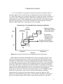


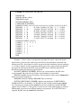

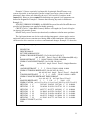

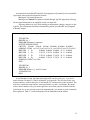
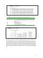
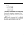
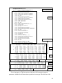

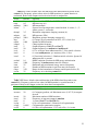

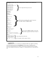
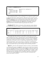
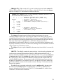
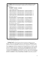
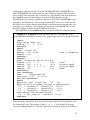
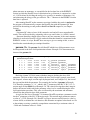
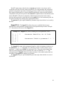
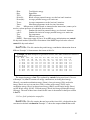
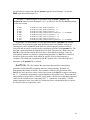

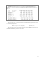

![Analyse de la tenue sismique des grands réservoirs[...]](http://vs1.manualzilla.com/store/data/006357607_1-f6d301e5706d64d4958f6a452af28255-150x150.png)
![Analyse de la tenue sismique des grands réservoirs[...]](http://vs1.manualzilla.com/store/data/006368585_1-4feb7f2835e3550c2e93b139d9c7a1e0-150x150.png)