No category

Download User Manual version 1.5

100

101

102

103

104

105

106

107

108

109

110

111

112

113

114

115

116

117

118

119

120

121

122

123

124

125

126

127

128

129

130

131

132

133

134

135

136

137

138

139

140

141

142

143

144

145

146

147

148

149

150

151

152

153

154

155

156

157

158

159

160

161

162

163

164

165

166

167

168

169

170

171

172

173

174

175

176

177

178

179

180

181

182

183

184

185

186

187

188

189

190

Transcript

software for the detection and analysis
of geographic boundaries
©BioMedware 2013
User Manual
version 1.5
©2013, BioMedware, Inc. All rights reserved.
BoundarySeer is a trademark of BioMedware, Inc.
Project Leaders: Geoff Jacquez and Susan Maruca
Software developers: Andrew Kaufmann, Lee Muller, Bob Rommel, Samik
Sengupta, and Prasheen Agarwal.
Help authors: Dunrie Greiling, Kim Hall, Susan Maruca, and Geoff Jacquez
Advisors and Beta-Testers: Dan Brown, Marie-Josee Fortin, Richard Hoskins,
Kim Lowell, Andrew Marcus, John Nuckols, and Stephanie Weigel.
This project was supported by grant # CA69864 from the National Cancer
Institute to BioMedware, Inc. The software and manual contents are solely the
responsibility of the authors and do not necessarily represent the official views of
the National Cancer Institute.
The software includes a modified version of Qhull from the National Science and
Technology Research Center for Computation and Visualization of Geometric
Structures at the University of Minnesota (www.geom.umn.edu).
The JPEG reader for this software is based in part on the work of the Independent
JPEG Group.
Support for TIFF file formats is based on work by Sam Leffier, ©1988-97 Sam
Leffier and ©1991-1997 Silicon Graphics, Inc.
The high spatial resolution hyperspectral data used in the development of the
software and in this manual (Figures 4.1 & 4.2) was provided by Yellowstone
Ecosystem Studies, which received funding support from the NASA Stennis Space
Flight Center Hyperspectral EOCAP.
For updated troubleshooting information and FAQs, please visit BoundarySeer
online (http://www.biomedware.com/files/documentation/boundaryseer/default.htm).
2
Table
Table of Contents
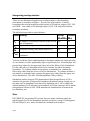
System requirements .............................................................................. 9
Manual overview ................................................................................. 10
CHAPTER 1—
1—INTRODUCTION
INTRODUCTION ..........................................
.......................................... 11
What are boundaries?........................................................................... 12
Boundary methods overview ................................................................ 13
Boundary analysis guidelines................................................................ 15
Examples of boundary analysis............................................................. 17
CHAPTER 2—
2—MANAGING AND
AND VIEWING DATA ............... 19
Projects overview ................................................................................. 22
Working with projects .......................................................................... 23
The project window ............................................................................. 24
About the project log............................................................................ 25
Working with the project log ................................................................ 25
M APS
Maps overview .................................................................................... 27
Working with maps.............................................................................. 29
The map toolbar .................................................................................. 30
Querying maps .................................................................................... 31
Interpreting color composite maps ........................................................ 32
F ORMATTING M APS
Formatting maps.................................................................................. 33
Line layer properties ............................................................................ 33
Point layer properties ........................................................................... 34
Polygon layer properties ....................................................................... 35
3
Raster layer properties.......................................................................... 36
T ABLES
Working with tables ............................................................................. 37
Querying tables.................................................................................... 38
C HARTS
Working with histograms ..................................................................... 39
Working with scatterplots..................................................................... 40
CHAPTER 3—
3—WORKING WITH
WITH SPATIAL DATA..................
DATA..................41
41
Adding or removing data from projects ................................................. 44
Data sets created in BoundarySeer ........................................................ 44
Data formats - raster, vector, and transect ............................................. 45
Data types - numeric, categorical, label ................................................. 46
Spatial features .................................................................................... 47
Missing data ........................................................................................ 48
Coordinate systems .............................................................................. 48
Data set properties ............................................................................... 49
Boundary properties............................................................................. 50
I MPORTING DATA
Importing data..................................................................................... 51
Custom imports: multiple GRID files.................................................... 52
Import formats for vector data .............................................................. 53
Import formats for raster data ............................................................... 56
Georeferencing raster data.................................................................... 58
Selecting variables to import ................................................................. 59
E XPORTING
Exporting data sets............................................................................... 60
Exporting cluster statistics .................................................................... 61
4
Exporting boundaries and subboundaries .............................................. 62
Exporting maps or charts...................................................................... 64
Exporting results.................................................................................. 64
CHAPTER 4—
4—PREPARING DATA FOR ANALYSIS .............. 65
Creating and using variable sets ............................................................ 67
Weighting variables ............................................................................. 68
Why standardize variables? .................................................................. 69
How to standardize your data............................................................... 69
Methods for data standardization ......................................................... 70
S PATIAL N ETWORKS
About spatial networks......................................................................... 71
Editing spatial networks ....................................................................... 73
Deactivating links using the mouse ....................................................... 73
Deactivating links using the minimum length option ............................. 74
Deactivating links using a spatial feature ............................................... 75
The spatial network toolbar .................................................................. 77
D ISSIMILARITY
About dissimilarity metrics................................................................... 78
Choosing a dissimilarity metric............................................................. 79
F UZZY C LASSIFICATION
LASSIFICATION
About fuzzy classification..................................................................... 81
The fuzzy classification process ............................................................ 82
Choosing fuzzy classification parameters .............................................. 83
About k-means clustering ..................................................................... 85
How to create fuzzy classes .................................................................. 87
5
CHAPTER 5—
5—DETECTING BOUNDARIES ...........................88
........................... 88
About difference boundaries ................................................................. 89
About areal boundaries ........................................................................ 90
About boundary detection .................................................................... 91
Boundary Detection Advisor Diagram .................................................. 92
Boundary Detection Wizard................................................................. 93
CHAPTER 6—
6—SPATIALLY CONSTRAINED CLUSTERING
CLUSTERING ....94
.... 94
About spatially constrained clustering ................................................... 95
Choosing cluster number...................................................................... 96
How to find boundaries using clustering................................................ 98
Interpreting clustering output...............................................................100
Clustering methods: centroid versus linkage .........................................101
Subsampling during linkage clustering .................................................102
Merging clusters..................................................................................103
CHAPTER 7—
7—WOMBLING................................
WOMBLING................................................
................ 105
About wombling .................................................................................107
Raster wombling.................................................................................109
Irregular (point) wombling ..................................................................110
Categorical wombling .........................................................................111
Polygon wombling ..............................................................................112
Crisp vs. fuzzy wombled boundaries ....................................................113
Thresholds..........................................................................................114
Thresholds..........................................................................................115
Subboundaries ....................................................................................117
How to find boundaries using wombling ..............................................120
Defining thresholds using histograms ...................................................122
6
Imposing new thresholds.....................................................................124
Interpreting wombling tables ...............................................................125
Interpreting wombling maps: polygon data...........................................125
Interpreting wombling maps: point data ...............................................126
Interpreting wombling maps: raster data ..............................................127
CHAPTER 8—
8—LOCATION UNCERTAINTY
UNCERTAINTY ........................ 128
About location uncertainty ..................................................................129
About wombling with location uncertainty...........................................130
How to womble with location uncertainty............................................132
Location models .................................................................................133
Interpreting location uncertainty rasters ...............................................134
CHAPTER 9—
9—BOUNDARIES FOR FUZZY CLASSES...........
CLASSES........... 135
Detecting boundaries on fuzzy classes..................................................136
How to detect boundaries on fuzzy classes ...........................................138
Interpreting fuzzy classification output.................................................139
CHAPTER 10—
10—ANALYZING BOUNDARIES ...................... 140
Components of statistical methods.......................................................142
O VERLAP S TATISTICS
About overlap statistics .......................................................................143
Overlap test statistics...........................................................................144
How to conduct an overlap analysis.....................................................145
Examples of overlap analysis...............................................................146
Overlap results....................................................................................147
Interpreting overlap statistics ...............................................................148
S UBBOUNDARY S TATISTICS
About subboundary statistics ...............................................................149
7
Subboundary test statistics...................................................................150
How to calculate subboundary statistics ...............................................151
Subboundary results............................................................................152
Interpreting subboundary statistics .......................................................153
M ONTE C ARLO R ANDOMIZATIONS
Monte Carlo procedures......................................................................154
Types of randomization ......................................................................156
p-values ..............................................................................................157
Calculating Monte Carlo p-values........................................................158
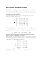
Using a generator matrix for randomization .........................................159
Calculating the generator matrix ..........................................................160
How the Generator Matrix Works: An Example ..................................162
RESOURCES ................................................................
....................................................................
.... 163
Glossary .............................................................................................164
Troubleshooting..................................................................................171
References ..........................................................................................174
Index..................................................................................................182
8
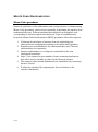
BioMedware's BoundarySeer detects and analyzes geographic boundaries with stateof-the-art techniques. BoundarySeer supports a range of data formats and types
and, through common file formats, can easily be used in conjunction with your
GIS.
System
System requirements
•
Windows 95 or Windows NT 4.0 or more recent operating system
•
screen resolution of 800 x 600 or finer for best viewing of the maps and
graphics
•
256 colors or better highly recommended for graphics
9
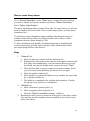
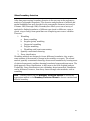
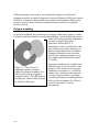
Manual overview
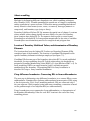
This manual outlines how to use BoundarySeer, BioMedware’s tool for detecting and
analyzing geographic boundaries. This information is also available in online help
("BoundarySeer Help.chm"), accessible from the "Help" menu and "Help"
buttons on dialogs in BoundarySeer. The online help has hyperlinks which
connect related topics.
BioMedware also has a BoundarySeer Online page on its website,
http://www.biomedware.com/files/documentation/boundaryseer/default.htm
Please check this for updates and additional information.
Chapters 1-4 describe the conceptual background, the interface, and how to
prepare your data for analysis. Chapter 1 outlines boundary detection and
analysis. Chapter 2 details the interface and data and boundary visualization tools
available, like maps, tables, and charts. Chapter 3 covers working with spatial data
in BoundarySeer, describing data formats, types, import and export, and
conventions for missing data. Chapter 4 itemizes methods to prepare your data for
boundary detection. Possible preparations include creating and using variable sets,
weighting variables, standardizing your data, editing spatial networks for point
data, and classifying your data.
Chapters 5-9 deal with the heart of BoundarySeer: boundary detection methods.
Chapter 5 introduces the concepts and features a boundary detection advisor,
available in an online version as well. The advisor should help you determine
which method is best suited to your questions and your data. Within the software,
you may use the Boundary Detection Wizard to choose a method and find
boundaries. Chapters 6-9 describe individual boundary detection methods.
Chapter 10 summarizes boundary analysis methods in BoundarySeer:
subboundary and overlap analysis.
The manual also has a resources section that includes a glossary, troubleshooting,
references, and an index.
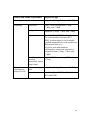
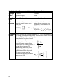
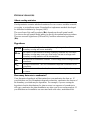
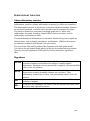
For easier differentiation of interface and description, this manual will use the
following style conventions:
Typeface
serif type
sans serif type
10
Meaning
explanatory text
part of the BoundarySeer interface, such as
menu items or dialogs
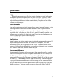
C HAPTER 1— I NTRODUCTION
BoundarySeer offers a number of methods for delineating and then analyzing
boundaries. This chapter provides an overview of the software and important
concepts. Essential concepts include definitions of the types of boundaries you can
delineate using BoundarySeer and short descriptions of the methods to find them.
This chapter also includes some background on the field of boundary analysis,
such as guidelines for planning data collection and analysis and examples from the
literature.
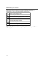
What are boundaries?........................................................................... 12
Types of boundaries.................................................................................... 12
Characteristics of boundaries....................................................................... 12
Boundary methods overview ................................................................ 13
Boundary detection .................................................................................... 13
Delineation of areal boundaries ........................................................................... 13
Delineation of difference boundaries.................................................................... 13
Fuzzy Classification ................................................................................... 14
Boundary Analysis ..................................................................................... 14
Subboundary statistics ........................................................................................ 14
Overlap statistics................................................................................................ 14
Boundary analysis guidelines................................................................ 15
Scale of sampling........................................................................................ 15
Choice of variables ..................................................................................... 15
Making sense of boundary analysis .............................................................. 16
Examples of boundary analysis............................................................. 17
Epidemiological applications....................................................................... 17
Ecological applications ............................................................................... 18
11
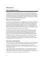
What are boundaries?
You might think of a boundary as a set of connected spatial locations that separate
areas with different characteristics. For example, a boundary for a toxic waste site
separates areas of high pollutant concentration from adjacent areas of low
concentration. A boundary for a species' range delineates where the species is
found and where it is not. An economic boundary distinguishes a poorer
community from a wealthier one.
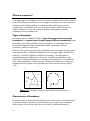
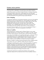
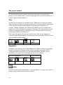
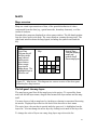
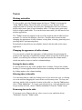
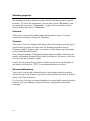
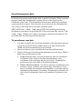
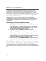
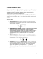
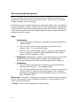
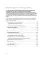
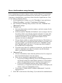
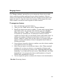
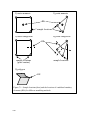
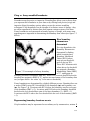
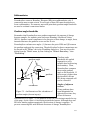
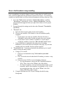
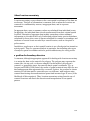
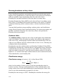
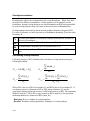
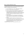
Types of boundaries
Boundaries may be formally defined as edges of homogeneous areas (areal
boundaries) or as spatial zones of rapid change (difference boundaries). Areal
boundaries are closed and fill the study area (Figure 1.1a). Examples of areal
boundaries include the edges of agricultural fields, watersheds, political
boundaries, and forest clear-cuts.
However, the processes that give rise to boundaries are not always associated with
homogeneous areas. Difference boundaries, zones of rapid change, describe this
situation. A cliff edge illustrates a difference boundary—the edge marks a
potentially dangerous difference in elevation. For difference boundaries, the
values of the variable immediately to one side of the boundary are very different
from values immediately to the other side. Difference boundaries are often open,
meaning that they appear as line segments that do not enclose an area (Figure
1.1b).
(a )
(b )
1
2
4
3
5
Figure 1.1 Examples of areal (a) and difference boundaries (b).
Characteristics of boundaries
Boundaries may be further distinguished by other characteristics. Boundaries may
be natural (such as a shoreline) or artificial (such as a road). Some boundaries,
such as edges of forest clear-cuts, may not be easily classified as natural or
12
artificial. Boundaries may be crisp (well defined) or fuzzy (imprecise). Both areal
and difference boundaries can be fuzzy. Fuzzy boundaries occur when the zone of
change from one type to another is relatively wide. Additionally, boundaries may
be generated by a single variable, such as the concentration of a toxin, or by a suite
of related variables, such as ecotones defined by multiple species' densities.
Boundary methods overview
You can use BoundarySeer to detect and then to analyze boundaries on your data.
Boundary detection
The choice of a boundary delineation method depends on your research question
and your data type. Boundary detection methods differ for areal and difference
boundaries. Although the different techniques will likely yield boundaries in
similar locations, they indicate different (but related) types of spatial patterns.
Choose your method with their distinctions in mind.
See also: About boundary detection.
Delineation of areal boundaries
Within BoundarySeer, you can use spatially constrained clustering to delineate
areal boundaries. First, it identifies homogeneous areas, then it draws boundaries
separating these areas. BoundarySeer can use one of two clustering methods to
assign locations to clusters based on the relative similarity of the values of variables
and geographic adjacency. The result is a partition of the data into relatively
homogeneous clusters.
See also: About spatially constrained clustering
Delineation of difference boundaries
Difference boundaries are zones of rapid change. You can use Wombling methods
to delineate difference boundaries. Wombling methods first estimate the average
amount of change in the variable(s) across space (referred to as a Boundary
Likelihood Value - BLV). The locations that have BLVs above a user-set threshold
value are referred to as Boundary Elements (BEs).
Adjacent crisp BEs that have similar amounts and directions of change are
connected into subboundaries. Because fuzzy boundaries consist of BEs with
varying boundary membership, BoundarySeer does not connect fuzzy BEs into
subboundaries. The collection of subboundaries and singleton BEs together are the
"boundary."
See also: About wombling, Crisp vs. fuzzy wombled boundaries, and About
13
wombling with location uncertainty.
Fuzzy Classification
Fuzzy classification can be used to reduce the dimensionality of a large data set. It
can be used to find groups—classes—in the data based on values of the variables.
Fuzzy classes are suitable for continuous data that do not fall out into discrete,
crisp classes.
In a crisp classification, each sampling location belongs fully to one class only.
With fuzzy classification, membership in classes can be partial. In other words, a
location may belong most strongly to one class, but have a lesser relationship with
other classes; or, it may belong rather equally to all classes. Boundaries can then be
detected on fuzzy classes using wombling, or boundaries can be described by
locations with high class uncertainty, using the classification entropy or confusion
indices.
See also: About fuzzy classification.
Boundary Analysis
BoundarySeer offers two techniques to analyze boundaries once you have
delineated them: subboundary and boundary overlap statistics.
Subboundary statistics
Subboundary statistics address the question, 'Are the boundaries significantly
contiguous?' Subboundary statistics can also indicate boundary 'branchiness', a
form of boundary complexity.
See also: About subboundary statistics.
Overlap statistics
Overlap statistics evaluate the spatial association between two sets of crisp
boundaries, based on average minimum distances from BEs in one set to BEs in
the other.
See also: About overlap statistics.
14
Boundary analysis guidelines
Boundary analysis is appropriate in the exploratory stage and the hypothesis
testing stage of research. During initial data exploration, boundary analysis can
identify spatial patterns and generate testable hypotheses. Designing experiments
for hypothesis testing requires more careful planning and a more thorough
understanding of the analytical techniques to be used. Along those lines, we offer
the following guidelines for hypothesis testing using BoundarySeer.
Scale of sampling
An important consideration in any spatial investigation is the scale of the sampling
framework. By scale we mean both the size of the geographic area under study,
and the spatial intervals at which observations are made. Ideally, the scale of the
sampling regime reflects the scale of the processes under investigation.
Determination of the appropriate scale may require a pilot study or other
preliminary work. A sampling regime that is too broad or too narrow for the
relationships under study will likely result in failure to detect boundaries or
associations that may actually exist. In the event of non-significant findings, a
logical first question is, 'Was the scale appropriate for this study?'
Choice of variables
Within BoundarySeer, boundaries may be delineated based on one or many
variables measured at a set of study locations. For example, in ecology, ecotones
(boundaries between adjacent ecosystems) may be delineated based on changes
across space in the abundance of one dominant plant species, or based on changes
in many plant species. The corresponding data sets would consist of data
representing the abundance of plants measured within some unit of area at each
spatial location. The first example would have only one variable for the focal
species, while the second would have a column for each species sampled.
Selection of variables to include in a data set should start with existing knowledge
of the system. Once a set of candidate variables has been constructed, a
combination of techniques may be used to decide which variables are included in
the boundary analysis. The first method is to look for boundaries for single
variables, evaluating each variable independently. Then, select variables for a
multivariate boundary delineation based on some predetermined criteria. For
example, you may include only those variables that have significant boundaries
themselves (determined using subboundary analysis), or you may include those
variables that have high rates of change in the same vicinity.
An alternative method is to use multivariate techniques such as principal
components analysis (PCA) to determine which of several candidate variables
15
contribute significantly to the overall variation in the system. You might then
decide to include variables that account for a certain proportion (e.g. 90%) of this
variation. In any case, let the research question or process model, rather than
models of data alone, guide selection of variables.
Making sense of boundary analysis
Boundary overlap statistics address the question, 'Are boundaries for two data sets
significantly close to each other?' Implicit in this question is the assumption that
boundaries exist for the two suites of variables. Thus, boundaries must first be
evaluated before assessing overlap.
For difference boundaries, we suggest you evaluate this assumption by first
calculating subboundary statistics for each data set. Subboundary statistics will
assess boundary contiguity. If contiguous boundaries exist, then the interpretation
of boundary overlap is clear: discrete boundaries overlap. If clear boundaries do
not exist within each data set, yet overlap is significant, then the two suites of
variables have a more complex relationship. In this case, areas of high rate of
change for each data set coincide. Further investigation may be needed to uncover
the nature of the relationship.
16
Examples of boundary analysis
Boundary locations reflect complex underlying physical, biomedical, and/or social
processes. Boundary analysis allows investigation of complex and dynamic spatial
processes.
Boundary analysis has been used to study genetic hybrid zones in population
biology (Endler 1977), where gene frequency boundaries exist at the interface
between populations; zones of rapid change in species abundance in ecological
communities (Fortin 1992); landscape boundaries in conservation biology (Hansen
and di Castri 1992; Fortin 1994; Holland et al. 1991), which represent contact
zones between distinct ecosystems; and retroviral molecular data (Bocquet-Appel
unpublished manuscript), which may lead to new hypotheses regarding gene
expression.
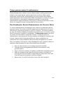
Epidemiological
Epidemiological applications
Bocquet-Appel (unpublished manuscript) applied boundary analysis to the
geographic distribution of retroviral mutations. He analyzed the env gene of
HTLV-1 retroviruses sampled from human populations at 22 African locations.
Boundary analysis revealed that zones of rapid change in the env gene overlaid the
geographic edge of the tropical rain forest, leading to new hypotheses regarding
env gene expression. He concluded that boundary analysis might be used to
explore spatial relationships between geographic zones of pathogen (e.g. ribovirus,
bacteria) molecular genetic variation and the spatial pattern of pathology in host
populations.
Another application is the identification of spatial boundaries demarcating zones
of rapid change in cancer mortality. These boundaries define the geographic extent
of areas with high mortality. Brown et al. (1995) conducted an etiologic study of
bladder cancer that used mortality maps to identify the study population. Other
areas of potential application include air pollution and respiratory illness (Bates
and Sizto 1983; Buffler 1988; Bates et al. 1990; Dockery et al. 1993),
environmental risk factors and cancers (Najem et al. 1985; Carpenter and
Beresford 1986; Jacquez and Kheifets 1993), and agricultural and industrial
exposures and cancer (Blot and Fraumeni 1977; Matanoski 1981; Stokes and Brace
1988; Linos et al. 1991; Nuckols et al. 1996).
Potential applications of boundary analysis within the relatively new field of
spatial epidemiology are numerous and rich. Zones of rapid change in cancer
outcomes can be caused by underlying differences in genetic composition, risk
behavior and environmental exposures. Thus, boundary analysis provides a basis
for formulating and testing spatio-epidemiologic hypotheses. Further, several
boundary detection methods are multivariate, and data for multiple diseases, such
17
as cancers at different body sites, can be analyzed simultaneously against exposure
data and genetic data from several loci. Boundary analysis has applications for
defining zones of rapid change in cancer outcomes (e.g. mortality); for determining
whether these zones are statistically unusual; and for testing them against
population genetic boundaries in oncogene expression and against edges of areas
with high carcinogen concentrations. However, to date applications in the analysis
of health data are relatively few. This lack of examples is at least partly attributable
to lack of familiarity with boundary analysis techniques.
Ecological applications
In ecology, boundary detection is appropriate for finding vegetation zones (Fortin
1994, Fortin et al. 1996, Fortin 1997), which is important in conservation and
planning and in other hypothesis-driven research. Boundary analysis is also the
ideal tool for investigating 'edge effects', which are differences in ecological
processes that occur at or near ecosystem or habitat boundaries. For example,
Kupfer et al. (1997) studied factors affecting woody species composition in forest
gaps in western Ohio, and found that composition was influenced not only by
commonly cited factors such as disturbance patterns and environmental measures,
but also by proximity to forest edges.
Forest fragmentation and population declines in Neotropical migrant birds
motivate recent work on edge effects on avian nest success in fragmented
landscapes. In a review of the accumulated research on the subject, Paton (1994)
found that although some studies report inconclusive results, there is substantial
evidence that nest success decreases in edge communities, due to increased brood
parasitism by Brown-headed Cowbirds and increased nest predation. Robinson et
al. (1995) monitored 5,000 nests in landscapes with varying levels of fragmentation
across the U.S. Midwest, and found that nest predation and mortality rates were
strongly and negatively correlated with percent forest cover. Donovan et al. (1997)
investigated the causes of variation in edge-effect study results, and suggested that
landscape context, host abundance, and predator assemblages can influence the
strength of such edge effects. Paton (1994) also explained that some research has
been compromised by relatively arbitrary edge detection techniques, highlighting
the need for more widespread use of appropriate boundary detection methods.
As an analytical tool, boundary analysis complements existing spatial techniques,
such as clustering and spatial autocorrelation analysis. Boundary overlap (Jacquez
1995) may be a more appropriate measure of spatial association than models such
as correlation and regression, which are built on the assumptions of linearity
and/or normality. Furthermore, boundary coincidence can be conducted for data
sets that do not use the same sampling regime, an advantage over other
techniques. For many research questions, boundaries and boundary overlap are
the logical objects of study.
18
C HAPTER 2— M ANAGING AND V IEWING D ATA
BoundarySeer organizes data and analysis into projects, which consist of the data
sets, boundaries, maps, tables, charts, and statistical results you generated. You
may save the project for work in another session.
BoundarySeer offers two work styles: a traditional approach using actions selected
from menus and an icon-oriented approach using the project window. In the iconoriented approach you can click on a data set and choose actions for BoundarySeer
to perform. This chapter describes the structure of projects in BoundarySeer and
its data and boundary visualization tools.
Projects overview ................................................................................. 22
Project components .................................................................................... 22
Working with projects .......................................................................... 23
Creating a new BoundarySeer project .......................................................... 23
Viewing and modifying project properties .................................................... 23
Selection color ................................................................................................... 23
Saving projects ........................................................................................... 23
The project window ............................................................................. 24
Data .......................................................................................................... 24
Boundaries................................................................................................. 24
Results....................................................................................................... 24
About the project log............................................................................ 25
Working with the project log ................................................................ 25
Editing....................................................................................................... 25
Hiding or showing ...................................................................................... 26
Printing ..................................................................................................... 26
Exporting................................................................................................... 26
M APS
Maps overview .................................................................................... 27
The left panel: the map layers ...................................................................... 27
The center panel: the map itself ................................................................... 28
The right panel: the legend .......................................................................... 28
19
Working with maps.............................................................................. 29
Creating maps ............................................................................................ 29
Adding layers to a map ............................................................................... 29
Changing the order of data layers................................................................. 29
Deleting map layers .................................................................................... 29
Removing maps.......................................................................................... 29
The map toolbar .................................................................................. 30
Querying maps .................................................................................... 31
Interpreting color composite maps ........................................................ 32
Red plus Green plus Blue = White ............................................................... 32
F ORMATTING MAPS
Formatting maps.................................................................................. 33
Line layer properties ............................................................................ 33
Thickness ................................................................................................... 33
Color ......................................................................................................... 33
Point layer properties ........................................................................... 34
Width ........................................................................................................ 34
Color ......................................................................................................... 34
Missing values ............................................................................................ 34
Polygon layer properties ....................................................................... 35
Line style ................................................................................................... 35
Color ......................................................................................................... 35
Raster layer properties.......................................................................... 36
Numeric rasters .......................................................................................... 36
Single color rasters..............................................................................................36
Color composite rasters: R,G,B............................................................................36
T ABLES
Working with tables ............................................................................. 37
Changing the appearance of table columns ................................................... 37
Sorting the data in tables ............................................................................. 37
Selecting data in the table ............................................................................ 37
20
Promoting data in the table ......................................................................... 37
Exporting tables ......................................................................................... 38
Querying tables.................................................................................... 38
C HARTS
Working with histograms ..................................................................... 39
Creating a histogram................................................................................... 39
Formatting and editing axis labels................................................................ 39
Formatting a histogram............................................................................... 39
Axes ................................................................................................................. 39
Bars .................................................................................................................. 39
Removing a histogram ................................................................................ 40
Working with scatterplots..................................................................... 40
Creating a scatterplot .................................................................................. 40
Formatting a scatterplot .............................................................................. 40
Axes ................................................................................................................. 40
Points ............................................................................................................... 40
Removing a scatterplot ............................................................................... 40
21
Projects overview
BoundarySeer organizes your work into projects, comprising multiple data sets,
boundaries, and results. When you save a project, BoundarySeer creates a *.bsr
file that contains all project components except spatial features. Spatial feature
information is saved in a file with a *.pip extension.
BoundarySeer uses projects for three reasons:
1. Projects simplify calculations that cross data sets, such as boundary
overlap.
2. Because BoundarySeer retains and stores information calculated from
data sets, the software avoids recalculating information such as spatial
networks and boundary likelihood values each time you delineate
boundaries or compute statistics, thereby improving efficiency.
3. Projects help organize and maintain data sets associated with your
analysis.
BoundarySeer project components
The following are components of BoundarySeer projects; all of these components
are saved into the project file (*.bsr) except spatial features. So, once you have
imported a data set into the project, you need not reimport it each time you open
the project in BoundarySeer.
Components:
Ÿ Data
Ÿ Cluster data
Ÿ Fuzzy class data
Ÿ Boundaries
Ÿ Spatial features
Ÿ Log
Ÿ Maps
Ÿ Charts
Ÿ Tables
Ÿ Results
Note: All project data sets should be associated with the same spatial location,
although each may contain different types of observations or different variables.
For example, you may wish to create a project comprised of two data sets for the
same study area, one with measurements on soil variables and another with
measurements on vegetation.
22
Working with projects
The basic functions related to working with and modifying projects are described
below.
Creating a new BoundarySeer project
When BoundarySeer first starts up, you have the option of starting a new project
or continuing work on an existing one. To start a new project, select that option,
and then you will need to import data. You may also create a new project at any
time by choosing New Project from the File menu.
Viewing and modifying project properties
To view the project properties window, go to the Project file, and then choose
Project Properties. The main "Properties" window provides space for you to
type in information about the creator of the project, and automatically provides the
creation date and the work directory. There is also space for adding notes in the
"Comments" box.
Selection color
The selection color is used in maps when you select items for map queries or links
for spatial network editing. You may change the selection color by clicking
"Change Color" and choosing another.
Saving projects
You can save projects directly from the File menu "Save Project" or "Save
Project As," or you can choose to save when you close a BoundarySeer session.
BoundarySeer project files (*.bsr) store the settings, data, boundaries, and results
created in a BoundarySeer session. When you reopen a saved project, you do not
have to reimport the source data.
23
The project window
The BoundarySeer project window provides an alternative to the pull-down
menus, an icon interface where you can simply right-click on data, boundaries, or
results to perform further analyses.
Data
Data
All data sets in the project are available on the "Data" tab of the project window.
Right-clicking on a data set brings up the menu list of data procedures. Some menu
choices are not available until preliminary steps have been completed. For
example, "Merge Clusters" and "Remove Clusters" are not available until
clusters have been established in constrained clustering. The selected data set is the
default for subsequent dialogs, although you may choose another from the pulldown menus within the dialog boxes.
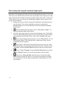
New icons will appear in the project window as new data sets are imported or
created through standardization or boundary detection procedures. Different icons
represent different data formats:
point data
polygon data
raster data
spatial features
Boundaries
Boundaries are displayed on the "Boundaries" tab. Right-clicking on a boundary
brings up a menu list of further actions, such as creating a histogram of BLVs,
changing boundary thresholds, or performing subboundary analysis. As new
boundaries are created, their icons appear in the project window.
Difference boundaries
point data
polygon data
Areal boundaries
raster data
all data formats
Results
Results are generated by subboundary or overlap analysis. You may view a table of
results or export them from the project window.
24
About the project log
As you work in BoundarySeer, the data you import, the methods you use, and the
settings you chose for the methods are all recorded on the project log. This feature
provides a detailed record of the analysis, so that you can recreate it or fine-tune it
in later BoundarySeer sessions, and so that you can interpret the results with full
knowledge of the sequence of analysis.
You may edit the log, print it, and/or export it to another application. Once
exported, the log can be opened with any text editor or word processor that reads
Microsoft Windows® rich text format.
Working with the project log
Your statistical output and a session log of BoundarySeer operations (e.g.,
boundary delineation, overlap analysis) are recorded on the Project Log, the memo
screen within the main window. The log text is stored within BoundarySeer in
Microsoft® Windows® rich text format. Throughout the course of your analysis,
you may find it useful to edit or print the text on this page. You can export the log
for opening in other applications.
Editing
1. Click on the Project Log window to activate it.
2. Select "Edit" from the main menu.
3. From here you can:
Ÿ Cut selected text to the clipboard (Cut), not active if no text selected
Ÿ Copy selected text to the clipboard (Copy)
Ÿ Paste text from the clipboard (Paste) not active if no text in clipboard
Ÿ Delete the selected text (Delete)
Ÿ Select all text on the page (Select All)
Ÿ Use a shortcut for adding the time and date to the log: Position the
cursor where you want the time and date to appear, then choose
"Time/Date"
Ÿ Mark selected text as a comment, /* like this */ (Comment)
4. You may also add references or notes directly to the session log page by

Microsoft® and Windows® are registered trademarks of Microsoft Corporation in
the United States and/or other countries.
25
positioning the cursor and typing.
Hiding or showing
Under the "Window" menu, you can choose to hide the project log. Later, when
you want to read the log, choose "show."
Printing
1. With the Project log active, select "File", then "Print" from the menu.
2. Click OK when the dialog box appears.
Exporting
The log is automatically saved within the *.bsr project file. If you wish to read it
in another application, such as a word processor or a text file reader, you can
export it as a text file (*.txt).
1. With the Project log active, select "File", then "Export" from the menu.
2. In the "Export" dialog, choose to export the Log.
3. As there is only one log in any BoundarySeer project, the list of all items
of that type will be blank. Select "Save" to continue saving the log.
4. Then, choose a name for the file and a location. BoundarySeer will save it
as a text file (*.txt).
26
MAPS
Maps overview
Maps are visual representations of data, of the spatial distribution of values
constructed from the data (e.g., spatial networks, boundary elements), or of the
results of analyses.
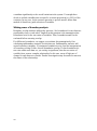
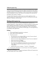
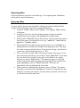
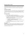
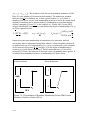
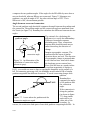
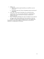
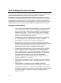
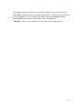
BoundarySeer maps are displayed in a three-pane window. The left-hand window
lists the active layers in the map. The center window contains the map itself. The
right-hand window shows the map legend, including the symbols used and the
key.
Map
Layer Pane
This pane lists all
the layers in the
map, with red
checks next to
layers that are
shown, empty
boxes next to
hidden layers. The
highlighted layer is
the active one.
Map
Legend Pane
This pane displays
names and
symbols for all
shown map layers.
Figure 2.1. Map layout. This diagram is a cartoon version of the three-pane
BoundarySeer map window.
The left panel: the map layers
The map layers panel lists all the map layers in the project. To expand the frame
and view the full layer names, drag the line between the layer names and the map
itself.
You may show or hide a map layer by checking or clearing its associated box using
the mouse. Displayed layers have a red check in the box next to their name.
The active layer, the one that is queried with the query tool, is highlighted on the
layers list. You can change the active layer by clicking on its name in the layer list.
To change the order of layers on a map, drag layers up or down the list.
27
The center panel: the map itself
The maps are drawn sequentially, with layers higher on the list overtopping those
lower on the list. For instance, if you have a polygon layer it may obscure a line
layer underneath it. To fix this, change the order of layers in the layer list.
The right panel: the legend
The legend identifies the symbols for active map layers.
28
Working with maps
Maps display sample locations, spatial networks, boundaries, and subboundaries.
Maps are not simply visual displays—they provide opportunities for querying the
underlying data. See also:
also Exporting maps or charts p. 61.
Creating maps
There are many opportunities to create maps when performing other actions in
BoundarySeer. To create (or re-create) a map outside of another action, choose
"Add to map" from the "Project" menu. First, select which component you will
add to the map. Then, choose "New Map" from the pull down list of all maps in
the project.
Adding layers to a map
ma p
There are many opportunities to add layers to existing maps when performing
other actions in BoundarySeer. You may also add data or boundaries to a map by
right-clicking on the object in the project window and choosing "Add to map"
from the pop-up window.
Changing the order of data layers
The left map pane lists the map layers. For a layer to be visible in the map
window, its associated box must be checked. Click on the box to check or clear it.
The data layers appear in the order that they are listed, with the top layer in the list
appearing "above" other layers in the view. To change the order of layers, click on
a layer in the list and drag it to where you want it.
Deleting map layers
If you want to completely remove a data layer from a map (not just deactivate it),
highlight the name of the layer, and then hit "Delete" on your keyboard. You
may also remove a layer by right clicking on the map and choosing to "Remove
this layer from the map." This method removes the active (highlighted) layer.
Removing maps
If you want to remove a map from a project, click on the "close" button
in the
map's upper right corner. This permanently removes the map. If you removed a
map in error, you may re-create it (assuming you have not also removed map
source information such as data or boundary layers).
29
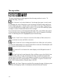
The map toolbar
The map visualization toolbar appears when the map window is active. To
activate the map, click on it.
The "selection" tool is the default tool. In the map layer pane, it can be used
for changing the order of map layers, and activating and deactivating map layers.
In the central map pane, it can be used to select items on the map. Using this tool
you can click directly on a single item to select it, or you can click and drag open a
rectangle to select all items that intersect the rectangle.
If you move the arrow to a the map pane and right-click, you will have the option
of querying the point, changing the properties (color, size of elements) of the data
layer, or removing the active (highlighted) layer from the map.
Use the "zoom" tool to focus on a section of the data set. Move the tool to
where you want to zoom, and click to zoom in.
Use the "zoom out" tool to enlarge the field of view. Move the tool to where
you want the enlargement to be centered and click to zoom out. BoundarySeer will
not zoom past the spatial extent of the data.
The "zoom to fit" tool returns the visual display to the full spatial extent of
the data set.
The "pan" tool can be used instead of the scrollbars to move the field of view
across the map. This tool only works when the map is zoomed in from the full
spatial extent of the data. Click on the button to activate the tool and then use it to
pan the map across the viewing window. For example, to expose a section to the
right of the viewing window, drag the map to the left.
Finally, the "query" button is a method for querying the map; clicking a point
with this tool brings up a table of information about the selected location.
30
Querying maps
Querying calls up information about items on the map.
Click on the query tool and then click on the map. This brings up a table of
information on the selected map layer (the highlighted layer). The selected layer is
queried even if it is not currently displayed on the map (checked in red). To change
the map layer queried, select a new layer in the map layers pane.
Once you've queried a layer, its table will pop up. This table lists information
about the point you've selected. For example, if you query a boundary layer, you
will get information on the location queried (queried x and y), the coordinates of
the closest Boundary Element (BE) to the queried point (point x and y), the
Boundary Membership Value for that BE, the average gradient magnitude (or
Boundary Likelihood Value - BLV) for all variables in the data set at that location,
and then BLVs and gradient angles for each individual variable in the data set at
that location.
If you have trouble understanding the information presented in a boundary query,
see the appropriate method description.
31
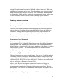
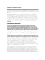
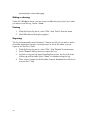
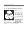
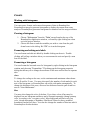
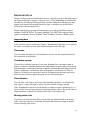
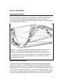
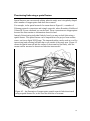
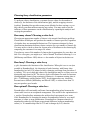
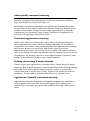
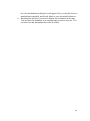
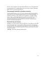
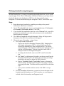
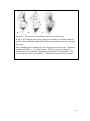
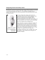
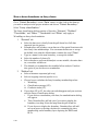
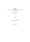
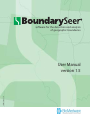
Interpreting color composite maps
Color composite maps display the values of up to three variables at one time. You
can make color composite polygon and raster map layers in BoundarySeer. In
color composites, each variable is displayed as gradations of a single color, red,
green, or blue. Interpreting these maps is straightforward, once you realize the
basic principles of combining colors of light.
Red plus
plus Green plus Blue =
White
red
fuschia
yellow
white
blue
cyan
green
Figure 2.2. Light/color blending
diagram. See this topic in the online help
for a full-color diagram.
Recall your high school physics
unit on light wavelengths. White
light consists of all wavelengths of
light together, while the absence of
light is darkness, black. Thus,
gradations of color in color
composite maps go from dark (low
values of all three variables) to light
(high values of all three variables).
Areas in a "pure" color (red, green,
or blue) have high values of only
one variable and low values of the
other two, while white areas have
high values of all variables, and
black areas are low in all.
Fuschia is a mixture of red and blue, with low values of the green variable; yellow
is high green and red, with low values of blue; and cyan is high green, high blue,
low red. Query the map to view the values of each variable.
32
F ORMATTING M APS
Formatting maps
To format a map layer, select it on the map layer pane (the selected layer is
highlighted).
Then, call up the properties dialog by right-clicking on the map with the
selector and choosing "Properties" from the pull-down menu. Because formatting
options change with the layer type, read up on individual layers.
Line layer properties
You may change the thickness and color of line layers on maps. Single value and
single color are the defaults, though graduated thickness and graduated color are
available for data sets that have more complexity. You may use line thickness and
color to represent two different variables. Many BoundarySeer line layers,
however, will be spatial features without associated data.
Thickness
You can choose to have all lines the same width (choose "Single thickness" and
the size in pixels from the drop-down box). Or, you may use the thickness of the
lines to indicate the value of a variable (choose "Graduated using single
variable"). If you choose graduated thickness, you need to choose a variable from
the drop-down list and choose the minimum and maximum thickness in pixels
from the lists.
Color
You can choose to color all lines the same (choose "Single color" and the color
using the "Change Color" button). You may also show the values for a single
numeric variable using graduated color. For graduated color, you choose the
variable and the minimum and maximum colors. The default is to grade from gray
to black, but you could choose any combination of minimum and maximum
colors, such as white to gray:
The last alternative is to color lines using the values of a categorical variable. Once
you choose the variable to represent, BoundarySeer will choose the colors.
33
Point layer properties
You may change the width of points, their color, and whether to display missing
values on the map. You may use point width and color to represent the values of
two different variables.
Width
You can choose to have all points the same width (choose "Single width" and
the size in pixels from the drop-down box). Or, you may use the size of the points
to indicate the value of a variable (choose "Graduated width using single
variable"). If you choose graduated width, you need to choose a variable from the
drop-down list and choose the minimum and maximum point sizes from the lists.
Color
You can choose to color all points the same (choose "Single color" and the color
using the "Change Color" button). You may also show the values for a single
numeric variable using graduated color. For graduated color, you choose the
variable and the minimum and maximum colors. The default is to grade from gray
to black, but you could choose any combination of minimum and maximum
colors, such as white to gray:
The last alternative is to color points using the values of a categorical variable.
Once you choose the variable to represent, BoundarySeer will choose the colors.
Missing values
Missing values are indicated with a special symbol on the map (the default symbol
is an empty circle with a red outline). You may choose not to show missing values
on the map, if so, clear the box at the bottom of the dialog.
34
Polygon layer properties
You may change the outline style and the fill colors of polygon layers.
Line style
You can choose the width of the lines and their color. Choose the width from the
drop-down box and the color using the "Change Color" button.
Color
You can choose to color all polygons the same (choose "Single color" and the
color using the "Change Color" button). You can also color them all
"transparent," this shows only the outlines and lets information from underlying
map layers come through.
You may color polygons using the values of a categorical variable. Once you
choose the variable to represent, BoundarySeer will choose the colors.
Alternatively, you may show the values for a single numeric variable using
graduated color. For graduated color, you choose the variable and the minimum
and maximum colors. The default is to grade from gray to black, but you could
choose any combination of minimum and maximum colors, such as white to gray:
You may choose to represent the values of up to three numeric variables using red,
green, and blue. You specify the value associated with each color.
35
Raster layer properties
Numeric rasters and categorical rasters have different properties. For categorical
rasters,
rasters you only have one format choice: you can select which variable to display
in the map. BoundarySeer chooses the colors automatically.
Numeric rasters
Single color rasters
Two features of monochrome raster layers can be changed in the dialog box: the
direction of the graduated color and the base color itself.
The raster will grade from a minimum to a maximum color value, with the
maximum value represented by the darkest color as a default (Maximum value:
Black). You may reverse it to have the lightest color as the maximum (Maximum
value: White) in this dialog.
You may also change the base color by clicking on "Change Color" and selecting
a new one from the spectrum.
Color composite rasters: R,G,B
Composite color rasters can display up to three variables or bands of remotely
sensed data on one map. The variables are represented by red, green, and blue.
These types of rasters are also called false color composites, as the colors on the
map do not necessarily correspond with those perceived by the human eye.
You may change the variables represented by each color in the raster properties
dialog box. You can choose the variables represented by each color (red, green,
blue) from pull-down lists in the raster properties dialog.
36
T ABLES
Working with tables
To view a table, go to the Project menu and choose "Table" to bring up the
"View Table" dialog. Choose the table you wish to view. Because of the
complexity and size of many raster data sets, BoundarySeer does not currently
display entire raster data or raster boundary tables. You may query raster map
layers to display small tables. To view the entire raster table, you will need to use
another application.
The "Table" menu only appears at the top of the window when a table has been
activated. To activate the window, click on it. Possible table actions include:
changing the appearance of table columns, sorting data, selecting, promoting rows,
querying tables, and exporting them.
BoundarySeer data tables are not editable. Instead, edit the table in the source
application.
Changing the appearance of table columns
You can stretch or shrink the appearance of table columns by positioning the
pointer at the right edge of a particular column. When you get the double-arrow
symbol, you can drag the column to the right and increase the column width,
which can make it easier to read the column headings.
Sorting the data in tables
To sort the data set by any of the variables that it contains, click on the column
heading. You can toggle back and forth between ascending and descending order
by clicking again on the column heading.
Selecting data in the table
You can select data in a table by clicking on a row (to select one row), or clicking
on a row and then dragging the cursor down to select many rows. To clear your
selection, simply click on another location in the table, or, from the Table menu,
select "Clear selection". To reverse your selection (e.g., select all data that were
not previously selected), choose "Switch selection" from the "Table" menu.
Promoting data in the table
To promote rows of data to the top, select a row or rows, and then choose
"Promote" from the "Table" menu.
37
Exporting
Exporting tables
Export methods are specific to each table type. See exporting data, boundaries,
and results for more information.
Querying tables
To query a table, first activate the table by clicking the pointer within the table
window. Then, follow the steps below to perform the query.
1. From the "Table" menu, choose "Query". The "Query Table" dialog
will appear.
2. At the top of the box, use the pull down menu to show the possible
variables that you can query, and highlight one variable name.
3. Pull down the "Operator" list in the next box, and choose the description
that fits the query you would like to do (e.g. "equal to," "less than or
equal to," "greater than").
4. Select whether the variable you are going to query on is a number or a
string (character variable) by clicking on the appropriate dot. Then type
the value or string in the box below. If you choose a string, you will need
to enter the value in double quotes (e.g., "A").
5. Next, you need to decide what to do with the results of the query. If you
haven't already selected any rows of data, choose "New Set." If you want
the rows that are the results of your query to be added to an existing
selected set, choose "Add to set." If you want the query to only look
within a selected set when choosing rows (leaving only the results of the
query highlighted), choose "Select from set." The rows are
immediately selected (highlighted) in the table.
6. When you have completed your selection, choose "Close." The values
that meet your query will be highlighted. If you have a large data set and
multiple rows meet your criteria, you may want to promote selected rows
to view them all at the same time.
38
C HARTS
Working with histograms
You can create, format, and remove histograms of data in BoundarySeer.
BoundarySeer may also generate histograms to display the output from some
analyses. BoundarySeer generates histograms for numeric but not categorical data.
Creating a histogram
1. Choose "Histogram" from the "Data" menu found at the top of the
BoundarySeer application window, or found by right-clicking on a data
set in the project window.
2. Choose the data set and the variables you wish to view from the pulldown boxes in the dialog. Hit "OK" to view the histogram.
Formatting and editing axis labels
You can format and edit axis labels by double-clicking on the axis. Doubleclicking will call up a window where you can rename the axis and specify a new
font for the label.
Formatting a histogram
You can format the bars and axes of a histogram by right clicking in the histogram
window and choosing "Properties." This brings up the histogram properties
dialog that allows you to change the attributes of the axes and the bars on separate
tabs.
Axes
To change the scaling on the axes, set the minimum and maximum value shown
for the X and the Y axes. You may also specify the number of tick marks for each
axis of the histogram, or BoundarySeer can set the tick marks automatically. To
change the thickness of the axes, choose a line thickness from the pull-down box
next to "Line thickness:".
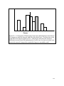
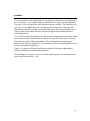
Bars
You may also change the color of the bars. Up to three colors of bars may be
displayed on one histogram and these can be changed separately (change primary
color, secondary color, or tertiary color). Most histograms will have only one
color, though histograms of Boundary Likelihood Values for fuzzy wombled
boundaries can have all three. You can also change the number of bins into which
BoundarySeer divides the data.
39
Removing a histogram
If you want to remove a histogram from a project, click on the "close" icon
in
the upper right corner. This permanently removes the histogram. If you remove a
histogram accidentally, you may re-create it (assuming you haven't also removed
other important files such as data or boundary layers).
Working with scatterplots
You can create, format, and remove scatterplots in BoundarySeer. BoundarySeer
may generate a scatterplot to display the output from some analyses.
BoundarySeer generates scatterplots for numeric but not categorical data.
Creating a scatterplot
1. Choose "Scatterplot" from the "Data" menu, found at the top of the
BoundarySeer application window or found by right-clicking on a data set
in the project window.
2. Choose the data set, the x, and the y variables from the pull-down boxes
on the dialog. Hit "OK" to view the plot.
Formatting a scatterplot
Axes
You may change the scaling on the axes by setting the minimum and maximum
value shown as well as the number of tick marks for the x and y axe s of the
scatterplot.
Points
You may also change the color and size of the points. BoundarySeer will display
an example of the new point format for your inspection. To accept the choice and
return to the chart, click "OK."
Removing a scatterplot
If you want to remove a scatterplot from a project, click on the "close" icon
in the upper right corner. This permanently removes the scatterplot. If you remove
a scatterplot accidentally, you may re-create it (assuming you haven't also removed
other important files such as data or boundary layers).
40
C HAPTER 3— W ORKING WITH S PATIAL D ATA
BoundarySeer projects begin with one or several spatial data sets. You can add
new data sets at any time by importing new data files into the project.
BoundarySeer supports two formats and two types of data. They are:
•
Data formats: raster, vector (point or polygon)
•
Data types: numeric, categorical
You also can generate additional data sets within the project by standardizing your
imported data sets, or through procedures such as fuzzy classification and spatially
constrained clustering.
This chapter describes how BoundarySeer handles data, data types and formats,
missing data, adding or removing data, and importing data. It also describes how
to export data, boundaries, tables, maps, or charts from BoundarySeer.
Adding or removing data from projects ................................................. 44
Adding data ............................................................................................... 44
Removing data ........................................................................................... 44
Data sets created in BoundarySeer ........................................................ 44
Cluster data sets ......................................................................................... 44
Fuzzy class data sets ................................................................................... 44
Data formats - raster, vector, and transect ............................................. 45
Raster ........................................................................................................ 45
Vector........................................................................................................ 45
Data types - numeric, categorical, label ................................................. 46
Numeric data ............................................................................................. 46
Categorical data ......................................................................................... 46
Binary data ................................................................................................ 46
Label/Other............................................................................................... 46
Spatial features .................................................................................... 47
Associated data .......................................................................................... 47
Applications............................................................................................... 47
Saving spatial features................................................................................. 47
Missing data ........................................................................................ 48
41
Choosing a missing value code .................................................................... 48
Missing values and boundary detection ........................................................ 48
Coordinate systems .............................................................................. 48
Data set properties ............................................................................... 49
Overview ................................................................................................... 49
Contents .................................................................................................... 49
Specifics..................................................................................................... 49
Boundary properties............................................................................. 50
Overview ................................................................................................... 50
Contents .................................................................................................... 50
Detection Information................................................................................. 50
I MPORTING DATA
Importing data..................................................................................... 51
Data name ................................................................................................. 51
Coordinate system ...................................................................................... 51
Data delimiter ............................................................................................ 51
Missing value code ..................................................................................... 51
Custom imports: multiple GRID files.................................................... 52
Import formats for vector data .............................................................. 53
Importing ArcView® shapefiles (points or polygons) ...................................... 53
Importing text files of point data .................................................................. 53
Importing BNA files ................................................................................... 54
Importing digital line graph files (DLG) ....................................................... 54
Importing MapInfo® interchange files (MIF, MID)........................................ 55
Import formats for raster data ............................................................... 56
Importing ENVI® files (BIL, BIP, and BSQ) ................................................. 56
Importing image file formats (TIFF, JPEG, BMP) ........................................ 56
Importing georeferenced image files (GeoTIFF and DRG files) ..................... 56
Importing DEM files................................................................................... 56
Importing GRID ASCII files ....................................................................... 56
Georeferencing raster data.................................................................... 58
To georeference your data ........................................................................... 58
42
Selecting variables to import ................................................................. 59
Selecting no variables.................................................................................. 59
Selecting variables ...................................................................................... 59
E XPORTING
Exporting data sets............................................................................... 60
Exporting cluster statistics .................................................................... 61
Exporting boundaries and subboundaries .............................................. 62
Exporting maps or charts...................................................................... 64
Exporting results.................................................................................. 64
43
Adding or removing data from projects
Adding data
When you first open a project, you will be asked to import some data for analysis.
Additional data can be imported into the project at any time. To add data, choose
"Import" from the "Data" menu, choose the type of data you want to add and
then follow the import dialogs.
For two different data sets to be analyzed together in BoundarySeer (i.e., used for
overlap analysis) they need to cover the same spatial area and be imported in the
same projection.
Removing data
You can remove data from a project by choosing "Project" from the main menu,
and then choosing "Remove". This will produce a list of the data sets in the
project that you could potentially remove.
We do not recommend removing data once you have used it for boundary
detection or analysis. In order to generate random boundaries for evaluation of
difference boundaries, BoundarySeer requires access to the original data set. The
original data are not needed for randomization of cluster boundaries, but to
preserve future flexibility in analyses we recommend keeping data in the project.
Data sets created in BoundarySeer
Cluster data sets
During spatially constrained clustering, BoundarySeer creates a cluster data set
associated with the original data set . The cluster data set is essentially a
categorical data set, where the categories are clusters.
Fuzzy class data sets
These types of files are created during fuzzy classification. They include the same
spatial information as the source file, but the variables represent class membership.
44
Data formats - raster, vector, and transect
BoundarySeer accepts raster, point, and polygon data sets. For all data formats,
the measured variables can be numeric, categorical, or label/other.
Raster
Raster data are sampled on a regular grid; that is, sample locations are
spaced at regular intervals in two spatial dimensions. Each data record is
comprised of X, Y, and values of the variable(s), where X and Y can correspond to
displacement or pixel numbers. Raster data are often generated from satellite
images or other remote sensing techniques.
Vector
BoundarySeer can detect boundaries for variables associated with points and
polygons.
Point data consist of X, Y, and values of variable(s).
Polygon data consists of vertices and associated data. Polygon files typically
come from a GIS, although users can create polygon text files in text editors for
importing into BoundarySeer.
BoundarySeer requires that the user import valid polygons, valid polygons in
BoundarySeer are non-overlapping and border each other (like the polygon icon to
the upper left). Polygons that do not share edges will not be recognized as
adjacent for boundary detection procedures like constrained clustering and
wombling. Polygons that overlap may not share a common edge, and may not
appear to neighbor each other. Also overlapping polygons may cause problems in
analyses like location uncertainty, for which points must be contained in only one
polygon.
Line data consists of vertices and associated data. Lines with associated data
cannot be used for boundary analysis, but they can be used as spatial features and
associated data can be viewed by querying the line layer on the map.
Similarly, point or polygon files without associated data cannot be used for
boundary analysis, but they can be viewed in the map and used as spatial features
for tasks like spatial network editing.
45
Data types - numeric, categorical, label
BoundarySeer supports three types of variables: numeric, categorical, and label.
All variables within a data set must be of the same type. If you try to import a file
with variables of different types, BoundarySeer will separate them into different
data sets, each containing only one variable type.
Numeric data
Numeric data are expressed as real numbers where the difference between two
numbers is mathematically meaningful. Examples include numbers of disease
cases, temperature, and salinity. Numeric data may be standardized so that each
variable is weighted equally in the boundary delineation process.
Categorical data
Values for a categorical variable represent membership of the sample in one of a
mutually exclusive set of categories. In BoundarySeer, categories must be
expressed as integers; however, the mathematical difference between two
categories represented by integers is not meaningful. That is, the difference
between 4 and 1 is the same as that between 2 and 1: both pairs are mismatched.
Examples of categorical data include blood type or soil classifications.
Binary data
Binary data are categorical data with only two categories. In BoundarySeer,
membership in binary categories must be expressed as either a "0" or "1". As with
categorical data, differences between values at different locations are described in
terms of matches or mismatches. Examples include species presence/absence,
survival, and status as a smoker or non-smoker.
Label/Other
You may have label variables that describe unique sampling locations, such as
your name for an area. You may wish to import these labels for your own use,
such as querying the map, even though they cannot be used in boundary analysis.
46
Spatial features
Spatial features are vector files that contain locations or spatial information
but may not have associated data, such as USGS DLG files. Typically, spatial
features provide locations of various natural or artificial boundaries or shapes to
help visualize spatial data and aid in network editing. They also can be used in
boundary overlap analysis.
Associated data
Lines with or without associated data are always treated as spatial features. Points
and polygons with or without associated data can be used as spatial features.
When you import spatial features, you can choose whether to import the
associated data. Even when the data will not be used for boundary analysis, you
still may want to visualize the data in the map. If you imported the data, you can
view it by querying the spatial feature map layer.
Applications
Spatial features can quicken spatial network editing by automating the removal of
inappropriate spatial network links. An outline of the study area, such as a
meandering stream, can be imported into the project. Then, this outline can be
used as a tool for selecting all links that occur outside of the study area, preventing
these locations from being included in later analyses.
Saving spatial features
Because spatial information without associated data cannot be used for boundary
analysis, BoundarySeer does not save spatial features with the rest of the project
file (*.bsr). Spatial feature information is saved in a *.pip file that needs to be
retained with the project file. The name of the spatial feature file will be the source
file name (e.g., "outline.dlg") with a *.pip extension (e.g., "outline.dlg.pip").
If you plan to use the information for network editing and not data visualization,
then you may wish to remove the spatial feature from the project once you have
edited the network. This way, you do not have to keep track of the *.pip file.
47
Missing data
With many remotely sensed files, pixels and/or entire regions can be recorded as
'no data' using a no-data or missing value code. In other data sets, such a code
might be used to indicate that the variable was not measurable at a location.
Choosing a missing value code
The missing value code should be a value that could not possibly show up as a true
data value in the data set. Often, codes such as "-9999" are used so that the code is
easy to recognize when you scan a column of data. Any integer value can be used,
including negative numbers. Currently, decimal values and text strings (such as
"no data") cannot be used.
Missing data in boundary detection
With multivariate data sets, BoundarySeer calculates gradients and distance
metrics using only those variables that have no missing values for all locations
involved. If a gradient or metric cannot be calculated because all variables have at
least one missing value for the locations involved, BoundarySeer will report the
missing value code as the metric (e.g. "-9999"). Further, when randomizing for
Monte Carlo procedures, BoundarySeer will not include those locations with every
variable coded as missing or 'no data'.
Coordinate systems
BoundarySeer can import data in planar coordinates, which includes all map
projections, and geographic (latitude-longitude) coordinates. All data sets in one
project need to be imported in the same projection, otherwise they will not register
properly for use in BoundarySeer.
1. Planar/Projection.
Planar/Projection This category comprises user-coordinates, UTM
(Universal Transverse Mercator), and other projection systems. You may
add the projection name when you import the data for your use, but
BoundarySeer does not distinguish between projections, nor does it
reproject anything other than geographic data. For this reason, you need
to import all project data sets in the same projection.
2. Geographic (latitude(latitude- longitude).
longitude) If your data are in geographic
coordinates, this information is recorded as part of the data set description
in BoundarySeer. Within BoundarySeer, data in geographic coordinates
are transformed to UTM for calculation and mapping purposes, but can
be transformed back for export (e.g. of data, boundaries, etc.) to other
programs.
48
Data set properties
To view data set properties, either choose "Properties" from the "Data" menu
and then choose the data set from the pull-down list. Alternatively, right-click on a
data set in the BoundarySeer project window and choose "Properties."
Overview
This section contains the name of the data set, its source file, date of modification,
and its coordinate system. Please note that BoundarySeer converts geographic
(latitude-longitude) data to UTM for calculation purposes.
You can change the data set's name by clicking on "Rename."
Contents
The lower left box varies for vector and raster data. For vector data, it lists the
form of the data (points or polygons) and the number of points or polygons
(features) in the data set. For raster data, you will see information on the height
and width of the raster in pixels.
For all data, BoundarySeer lists the number of variables and their labels. You may
rename variables by selecting the one you wish to change and then clicking
"Rename selected variable."
Specifics
The lower right box summarizes the data type (numeric or categorical), the
missing value code (if you entered one), whether the data set has been
standardized, whether the network has been edited (applies to vector point files
only), and whether it is a cluster or fuzzy class data set. If the data set contains
cluster or fuzzy class data, this box will also contain details about the clustering or
classification process. The "Standardized" box will be checked if you save
standardized variables into the original data set, or if you create a new
standardized data file.
49
Boundary properties
The boundary properties window provides detailed information about a specific
boundary. To access this information, you can either choose "Boundary" from
the menu and then choose "Properties", or right-click on a boundary in the
project window and choose "Properties."
Overview
This section, contains the boundary name and the parent data set. You may
rename the boundary by clicking on "Rename."
Contents
This section, lower left, displays information about the boundary itself: the type of
spatial feature (polygons for cluster data, for wombling data these may be
Delaunay triangles, polygon edges, or a number of other feature types depending
on the wombling method used).
Next, it lists the number of candidate boundary elements (cBEs), followed by the
number of Boundary Elements (BEs) found in the data set. For rasters, it also lists
the size of the raster (height x width).
Finally, the last item is the set of parent variables used to create the boundary. If
the variable is followed by "STD," it was standardized before analysis.
Detection Information
This section, bottom right, contains details of the boundary analysis procedure.
Besides the type (crisp or fuzzy), the specific method will be presented, as well as a
listing of all of the parameters.
For a review of the steps in creating boundaries, see individual boundary detection
methods, such as wombling, location uncertainty, and spatially constrained
clustering.
50
I MPORTING
MPORTIN G D ATA
When you first create a BoundarySeer project, a dialog pops up to ask what type of
data you would like to import—raster or vector. Then, depending on whether the
data file has a header describing the file's contents, additional dialog boxes may
appear that request information about the data, or whether you would like to
georeference the data (raster file).
When creating a new project in BoundarySeer, you will not be able to import
multiple Grid ASCII files. To import multiple Grid ASCII files with the same
spatial coordinates, choose "Import" then "Custom" from the "Data" menu.
Importing data
Once you have chosen a data set to import, BoundarySeer prompts you to specify
the name, coordinate system, and the data delimiter in the file type.
Data name
You can name the data set, or BoundarySeer will use the file name (without the
file extension) as the default.
Coordinate system
Choose the coordinate system of your data. BoundarySeer can import data in
planar coordinates (includes but does not differentiate between many projections)
and geographic coordinates (latitude-longitude). Because BoundarySeer works in
planar coordinates, it transforms data in geographic coordinates to UTM for
analysis. All data sets in one project need to be imported in the same projection,
otherwise they will not register properly for use in BoundarySeer.
Data delimiter
For text data, you need to choose the data delimiter (whether it is delimited by
tabs, spaces, or any whitespace, which can also include carriage returns).
Also, BoundarySeer needs to know whether to lump successive delimiters (e.g. a
series of tabs) or to interpret them as delimiting missing values. If you tell it not to
lump delimiters, it places the missing value code in the empty cells.
Missing value code
If you have or want missing values in your data set identified with a particular
code, enter that code here. Currently, decimal values and text strings cannot be
used as missing value codes.
51
Custom imports: multiple GRID files
The GRID format is a proprietary ESRI ® format for raster data that contains only
one variable. You may combine several GRID files into one BoundarySeer data
set. To do so, each file must contain numeric data, have the same header, and
cover the same spatial coordinates. At this time, categorical GRID files cannot be
imported and combined into one data set.
You cannot import multiple GRID files from the "Quick Start" dialog on
creating a new project in BoundarySeer. Cancel out of the "Quick Start" dialog if
you do not want any other data sets in your project.
1. To import multiple GRID files, choose "Import" and then "Custom:
multiple ARC/INFO® GRID" from the "Data" menu.
2. After you choose to import multiple GRID files, the "Import Raster
Data" dialog will appear. Choose the file type. Next, select the files to
import using the shift or control keys to select multiple files. Hit
"Import."
3. On the "Import Data" dialog
a. Choose a data set name (BoundarySeer chooses a name of one of the
files as the default).
b. Verify the coordinate system.
c. As GRID files are tab-delimited, the data delimiter section of the
dialog will be grayed out.
d. If a missing value code is specified in the header, then the missing
value section of the dialog will be blank. If not, choose a missing
value code.
e. Hit "Next"
4. Choose whether to view the data in a map (either a new or existing map).
ESRI® and ARC/INFO® are registered trademarks of the Environmental Systems
Research Institute, Inc.
52
Import formats for vector data
The import data option appears whenever you create a new project. You can
choose to import additional vector data sets at any time by choosing "Data" from
the main menu, and then choosing "Import Data", and then "Vector".
BoundarySeer can import vector files containing points, lines, and/or polygons.
BoundarySeer uses data associated with points and polygons for boundary
analysis. Lines and point and polygon files without associated data cannot be used
for boundary analysis, but they can be viewed in the map and used as spatial
features for tasks like spatial network editing.
BoundarySeer does not clean or verify polygon files on import. BoundarySeer
requires that the user import valid polygons, valid polygons in BoundarySeer are
non-overlapping and border each other (like the polygon icon to the upper left).
Polygons that do not share edges will not be recognized as adjacent for boundary
detection procedures like constrained clustering and wombling. Polygons that
overlap may not share a common edge, and may not appear to neighbor each
other. Also overlapping polygons may cause problems in analyses like location
uncertainty, for which points must be contained in only one polygon.
Available vector file types include: ArcView ® shapefiles, text files of point data,
BNA files, digital line graph files, and MapInfo® interchange files. When these files
are imported, BoundarySeer will ask you to identify which variables to include,
and their type (numeric, categorical, or label/other).
Importing ArcView ® shapefiles (points or polygons)
ArcView® shapefiles (extensions *.shp, *.shx, and *.dbf) can be imported
without modification.
Importing text files of point data
To import text files of point data, the files must consist of columns of data, with
each set of observations separated by a carriage return.
When BoundarySeer reads the file, it looks for information in a header (see
example below). You can add this header when creating the file, or BoundarySeer
will prompt you for the information during the import process. The header
information is not case-sensitive.
In the first line of the header, list the data type - this can be numeric or categorical.
On the next line, report the coordinate system. Currently, BoundarySeer
recognizes two coordinate systems: "planar" and "geographic" (latitudelongitude). On the next line, list the missing value code. On the last line of the
53
header, list the variable names in the order that they appear in the data file. These
names can be descriptive, e.g., canopy cover, contaminant concentration, etc., but
must be separated by commas.
The file itself consists of a list of observations for each location in the data set.
Each observation begins with the x coordinate, then the y coordinate. Next are the
values for each of the variables (separated by delimiters).
Data type: Numeric
Coordinate system: planar
Missing value: -99
Variable names: z1, z2, z3,
1
1
0.03 72
1200
1
2
0.05 85
1650
1
3
0.06 89
1650
1
4
0.08 -99 1750
z4
2.1
1.8
2.2
2.5
Importing BNA files
BNA files (*.bna), which are typically associated with Atlas GIS ® systems, can be
imported without modification. Often, these files are geographic (latitudelongitude) coordinates, although they may also be in UTM units.
Typically, these files do not contain variable names, and they have a maximum of
three variables. When the file is imported, BoundarySeer creates field labels for
each variable (e.g., "field 1", "field 2", up to "field 3"). When you import the file,
you will need to know how many variables to select, and the data type (numeric or
categorical) for each one. You can rename the variables in the data set properties
dialog.
If you need to examine the file to determine the number of variables and the
projection, these files can typically be opened in a text file reader.
Importing digital line graph files (DLG)
Digital line graph files (*.dlg) are digitized topographic or planimetric maps
available from the United States Geological Survey. These files contain images of
spatial features, such as topography, hydrography, and some political boundaries,
without associated data, so they cannot be used for boundary detection. DLG files
can be useful as a spatial feature for editing the spatial network of a related point
data set in BoundarySeer. The format is described in detail at the USGS website.
DLG files can be imported directly into BoundarySeer. At this time, BoundarySeer
supports import of "optional format" DLG files but not "spatial data transfer
standard" (SDTS) files.
54
Importing MapInfo ® interchange files
MapInfo® interchange files (*.mif, *.mid) can be imported directly. MapInfo®
interchange format consists of two files—the MIF file contains the graphics, while
the MID file contains the textual data. The MIF file header contains the details of
the coordinate system and bounds of the data set. BoundarySeer reads the
coordinate system information directly from the MIF file.
ArcView® and Atlas GIS® are registered trademarks of the Environmental Systems
Research Institute, Inc.
MapInfo® is a registered trademark of the MapInfo Corporation.
55
Import formats for raster data
The import data option appears whenever you open a new project. You can
choose to import additional raster data sets at any time by choosing "Data" from
the main menu, and then choosing "Import", and then "Raster". BoundarySeer
can import a number of raster data types, including ENVI® files (*.bil, *.bip, and
*.bsq), image files (*.tif, *.jpg), georeferenced images (GeoTiff and *.drg),
digital elevation models (*.dem), and GRID ASCII.
Importing ENVI ® files
ENVI® rasters can be saved in one of three different file formats, band sequential
(*.bsq), band interleaved by line (*.bil) and band interleaved by pixel (*.bip).
BoundarySeer can import any of these files directly, as it reads in the
georeferencing information in the header.
Importing image file formats
TIFF (*.tif) and JPEG (*.jpg) image files can be imported into BoundarySeer as
rasters. These files contain no georeferencing information, and so they must be
georeferenced on import or by using the georeferencing dialogs found from the
"Data" menu.
Importing georeferenced image files
GeoTIFF and digital raster graphics (*.drg) files are, essentially, georeferenced
TIFF files. These files are imported directly into BoundarySeer unless the file
contains insufficient georeferencing information.
Importing digital elevation model files
DEM files (*.dem) are USGS digital elevation model files that contain
georeferencing information. BoundarySeer can import these files directly.
Importing GRID ASCII files
The GRID format is a proprietary ESRI® format for raster data. GRID files
contain only one variable, although you may import several GRID files with the
same spatial coordinates.
To import GRID ASCII files, the file must begin with a header - the first 5 lines in
the header are required, while the sixth (listing a value assigned to missing data) is
optional. The first 5 lines should appear automatically when the file is generated
from ARC/INFO®, but if you are having trouble importing files, this may be the
56
source of the problem.
ncols
nrows
xllcorner
yllcorner
cellsize
NODATA_value
28
28
307420
5396980
30
-9999
In the example file fragment above, the first two header lines describe the number
of rows and columns in the file, and the next lines provide the coordinates for the
raster that represents the lower left corner of the data set. Some files present
"xllcenter" instead of corner - this is an acceptable format as well. The next
header line provides the cell (pixel) size, and the optional sixth line is for the
missing value code. After the header, the string of data for each cell appears,
starting in the upper left corner of the grid, with each value separated by a space
(space delimited) and each row separated by a carriage return.
See also: Georeferencing raster data, Data set properties, Missing data
ESRI® and ARC/INFO® are registered trademarks of the Environmental Systems
Research Institute, Inc.
ENVI® is a registered trademark of Better Solutions Consulting LLC.
57
Georeferencing raster data
Georeferencing means connecting the data to spatial coordinates. When you have
imported raster data, BoundarySeer requires the size of the pixels and the
coordinates of the raster. This information fixes the raster within the coordinate
system specified on import. Once the raster is georeferenced, then BoundarySeer
can overlay it with other files in the same coordinate space.
GRID ASCII files, *.dem, *.drg, and geoTIFF files include georeferencing
information in the data or in the header file. Other raster data files, such as *.bil,
*.bip, *.bsq, *.bmp, and *.jpg, do not always contain this information. For
these data files, the raster must be georeferenced.
To georeference your data
1. You may encounter the Georeferencing dialog in the data import process,
or you can access it from the "Data" menu or by right clicking in the
"Data" tab on the BoundarySeer project window.
2. Choose the data set to be georeferenced from the pull-down menu.
3. Choose which type of georeferencing information you will enter. Either is
sufficient to georeference the data.
a. Origin and cell size. You can georeference either by entering the
coordinates of the origin of the raster (the minimum x and y
coordinates of the grid edge) and the grid cell size. BoundarySeer
georeferences the entire data set from this information.
b. Raster data boundaries. You need to enter the coordinates for the
northern, eastern, southern, and western edge of the data set. This
data is essentially the minimum and maximum x coordinates and the
minimum and maximum y coordinates. BoundarySeer calculates cell
size from this information, based on the number of columns in your
data.
58
Selecting variables to import
In this dialog, you can choose to import all, some, or none of the variables in the
source file. Some data files may contain many more variables than you actually
wish to analyze, particularly if you intend to use the data for spatial network
editing.
Selecting no variables
In the case of spatial features, you may want to import only the spatial information
without other data. In that case choose "Do not import variables" and then
click "Next." BoundarySeer will import the spatial information without associated
data.
Selecting variables
1. Choose "Import variables" (the default choice).
2. Select variables to import by clicking on them and then move them from
the "Data source variables" box to "Variables to import" using the
"Add" button. Add the source variables to one of the three categories
(numeric, categorical, label/other).
a. If the header of your file has already identified the data type,
inappropriate data types will be grayed out.
b. If you move a variable into the wrong category, use the back arrow to
take it out again.
3. Once you have finished adding variables, click "Next" to continue the
import process.
Please note:
BoundarySeer is not yet able to work with variables of different types in the same
data set. If you import some variables of each type, BoundarySeer will create two
different data files, one for the categorical data and one for the numeric data.
Labels will be included in each file.
59
E XPORTING
Exporting data sets
Data sets imported into or created within BoundarySeer can be exported for use in
a GIS.
Source data Export file type
format
point data text (*.txt) OR shapefiles (*.shp, *.shx, and *.dbf)
polygon
shapefiles (*.shp, *.shx, and *.dbf)
data
raster data Grid ASCII files (*.txt).
Grid ASCII files only hold one variable, so BoundarySeer generates a
*.txt file for each one. The base name for the set of files is chosen in
the "Save As" dialog.
1. To export a data set, go to the "File" menu and select "Export" to bring
up the "Export" dialog box. Alternatively, right click on a data set in the
data tab of the project window and choose "Export" from the pop-up
menu.
2. From the pull-down list, choose to export data.
3. A list will appear of all of the data sets in your project. Choose the data set
you would like to export.
4. The coordinate system of your data is presented in the "Coordinate
system" box. If your data were automatically converted to UTM
coordinates from geographic coordinates (latitude-longitude), you have
the option of changing them back when you export.
5. Select "Save As."
6. A new window will appear that allows you to choose where to save the
file and its name.
7. The export format appropriate for your data will appear in the "Save as
type" box. Once you have selected a location and a file name, select
"Save".
60
Exporting cluster statistics
Files of cluster statistics include the cluster label, the number of elements within
the cluster, and the mean and variance of the variables used in clustering (if you
standardized the data before clustering, those variables will have STD after their
name). There is also a clusters data set, which can be exported like any other data
set.
Cluster statistics are exported as text files (*.txt). There are two ways to export
cluster statistics, one using the menu and the other using the project window.
1. Menu
a.
To export cluster statistics go to the File menu on the application
window and choose "Export."
b. Choose the type of item to export (Cluster statistics) from the
list.
c. Skip to step 3.
2. Project window
a. Right click on the Clusters icon in the Data tab.
b. Choose "Export" and then "Cluster Statistics."
c. Skip to step 3.
3. End of both methods
a. When you select the type, a list will appear of all of the items of
that type that are in your project. Highlight the set of cluster
statistics you want, and select "Save As."
b. A new window will appear that allows you to choose where to
save the file and its name.
c. Once you have selected a location and a file name, select "Save."
61
Exporting boundaries and subboundaries
Boundaries created in BoundarySeer can be exported for use in a GIS.
1. To export a boundary, go to the File menu or right-click on the boundary
in the project window and chose "Export".
2. In the "Export" dialog, choose to export a boundary on the pull-down
menu.
3. When you select boundary, BoundarySeer will list all boundaries in your
project. Select the boundary you want to export.
4. The export file format varies with the boundary type (see table below).
5. The coordinate system of the boundary is presented in the "Coordinate
system" box. If BoundarySeer converted your data from geographic
(latitude-longitude) data to UTM on import, you have the option of
changing them back when you export.
6. Select "Save As."
7. A new window will appear that allows you to choose where to save the
file and its name. For export types consisting of multiple files, the name
you choose will serve as the base name for the file set, with individual files
differentiated by what they contain. (e.g. for BLV, "basename
BLV.txt").
8. The export format appropriate for your data will appear in the "Save as
type" box. Once you have selected a location and a file name, select
"Save".
62
Source data format or procedure
Export file type
clustering on any data format
shapefiles (*.shp, *.shx, and *.dbf)
wombling
point data
text (*.txt) OR shapefiles (*.shp,
*.shx, and *.dbf)
polygon data
shapefiles (*.shp, *.shx, and *.dbf)
raster data
Arc/Info Grid ASCII files (*.txt): one
for each boundary descriptor (BLV,
BMV, gradient angle for each variable,
gradient magnitudes for each variable in a
multivariate data set).
For those with subboundaries:
subboundary connections exported in
shapefile format (*.shp, *.shx, and
*.dbf).
fuzzy
classification
using CI or CE
wombling with
location
uncertainty on any
data format
Grid ASCII file containing BMV values
(*.txt)
point or polygon
data
shapefiles (*.shp, *.shx, and *.dbf)
raster data
Arc/Info Grid ASCII files (*.txt) for
BLV and BMV.
63
Exporting maps or charts
Maps and charts created in BoundarySeer can be exported as bitmaps (*.bmp) for
use in a variety of word processing and drawing programs. BoundarySeer will
export the map and the legend, but not the layer list.
To export a chart or map, go to the File menu, and chose "Export."
1. In the "Export" dialog, choose the type of item to export (either a map or
a chart).
2. When you select the type, a list will appear of all of the items of that type
that are in your project. Highlight the chart or map that you want, and
select "Save As".
3. A new window will appear that allows you to choose where to save the
bitmap and its name.
Once you have selected a location and a file name, select "Save".
Exporting results
To export results, you can right-click on the set you want to export in the results
tab of the project window and choose "Export." Alternatively, go to the "File"
menu and select "Export" to bring up the "Export" dialog.
1. From the pull-down list, choose to export "Results."
2. A list will appear of all of the results in your project. Choose the results set
you would like to export.
3. Choose whether you want to standardize the output.
4. Select "Save As."
5. A new window will appear that allows you to choose where to save the
file and its name. Name the file and then select "Save." Results are
exported as text files (*.txt).
64
C HAPTER 4— P REPARING D ATA FOR A NALYSIS
After you have imported your data into BoundarySeer, and before you conduct
boundary analysis, you should consider preparing your data for analysis. This
chapter details methods to prepare your data within BoundarySeer, including
creating variable sets, weighting variables, standardizing data, editing spatial
networks for point data, classification, and dissimilarity methods used in boundary
detection.
Creating and using variable sets ............................................................ 67
Steps to create a variable set ........................................................................ 67
Editing variable sets .................................................................................... 67
Using variable sets ...................................................................................... 68
Weighting variables ............................................................................. 68
Why standardize variables? .................................................................. 69
How to standardize your data............................................................... 69
Methods for data standardization ......................................................... 70
S PATIAL N ETWORKS
About spatial networks......................................................................... 71
Why edit spatial networks?.......................................................................... 71
Editing spatial networks ....................................................................... 73
Editing modes ............................................................................................ 73
Deactivating links using the mouse ....................................................... 73
Deactivating links using the minimum length option ............................. 74
Deactivating links using a spatial feature ............................................... 75
Steps in deactivating links with a spatial feature:........................................... 76
The spatial network toolbar .................................................................. 77
D ISSIMILARITY
About dissimilarity metrics................................................................... 78
What are dissimilarity metrics?.................................................................... 78
Dissimilarity in BoundarySeer..................................................................... 78
Choosing a dissimilarity metric............................................................. 79
65
Numeric data ............................................................................................. 79
Categorical data.......................................................................................... 80
F UZZY C LASSIFICATION
About fuzzy classification..................................................................... 81
Why use fuzzy classes?................................................................................ 81
The fuzzy classification process ............................................................ 82
Steps.......................................................................................................... 82
Choosing fuzzy classification parameters .............................................. 83
How many classes? Choosing a value for k ................................................... 83
How fuzzy? Choosing a value for ϕ ............................................................. 83
How optimal? Choosing a value for ε ........................................................... 83
About k-means clustering ..................................................................... 85
How to create fuzzy classes .................................................................. 87
Steps.......................................................................................................... 87
66
Creating and using variable sets
BoundarySeer allows you to perform thorough investigations of multivariate data
sets by defining suites of variables for analyses. That is, you can select one or more
variables for boundary detection from a data set containing many variables. One
way that you might consider using this flexibility is for viewing boundaries based
on individual variables before combining them in a suite for multivariate boundary
analysis.
Steps to create a variable set
1. From the main menu, choose "Data", and then select "Variable Sets".
2. When the dialog box first opens, it shows the default variable set, which
includes all of the variables in a given data set. You cannot modify this
default set, but you may create a new set with different variables and/or
weights.
3. Choose the source data set for the variable set from the pull-down menu.
Remember, for a data set to appear in this window, you must have already
imported it into the project.
4. To create a new set, hit the "Create New Set" button. Enter a name for
the variable set or accept the default.
5. Then click the "Create New Set" button, and this name will be
displayed in the "Variable Set" window.
6. The new variable set begins with no variables (note that the "in set"
column in the table is empty). To add all of the variables, click the "Add
All" button. To add variables individually, click on the "in set" column,
which will put an "X" in the box. See Also: choice of variables.
7. To change the weight of an individual variable, type a new value in the
weight cell.
8. If you want to delete a variable set, select it from the pull down list, and
then click "Delete Set".
9. When you have created a variable set that you want to save, click
"Apply", and then close.
Editing variable sets
You can edit variable sets using the methods described above for creating variable
sets. Remember, you cannot edit the "All variables, equal weights" variable
set. You can change any variable set you have created by selecting it from the
drop-down list on the 'Variable Sets' dialog, and then changing which variables
are included or their weights. Remember to click "Apply" to save changes, and
67
then "Close."
You can also edit variable sets from within the Boundary Detection dialogs.
Using variable sets
When you want to conduct boundary analyses, these new variable sets will be
available for you to use. You will have the option to use or create variable sets
when you begin any BoundarySeer boundary detection method. Additionally, you
may select to use a single variable in any boundary detection method by filling in
the circle next to "Variable" (rather than Variable set) and then selecting your
variable.
Weighting variables
In BoundarySeer, you have the ability to give variables different weights prior to
the calculation of Boundary Likelihood Values. You can do this when you create
variable sets.
You may want to consider giving variables weights greater than one if you have a
reason for expecting that one or more of the variables contributes more strongly to
the boundary-generating process in a particular system than the other factors.
Another situation where you may want to weight variables is if you think two or
more variables are highly correlated, and you want to reduce their influence on the
analysis. In this case, you would probably give the variables weights that are less
than one.
68
Why standardize variables?
Many researchers have noted the importance of standardizing variables for
multivariate analysis. Otherwise, variables measured at different scales do not
contribute equally to the analysis. For example, in boundary detection, a variable
that ranges between 0 and 100 will outweigh a variable that ranges between 0 and
1. Using these variables without standardization in effect gives the variable with
the larger range a weight of 100 in the analysis. Transforming the data to
comparable scales can prevent this problem. Typical data standardization
procedures equalize the range and/or data variability.
How to standardize your data
1. Go to the "Data" menu choose "Standardize," or choose
"Standardize" from the menu that appears when you right click on a
data set in the project window.
2. Select a standardization method.
3. The standardized variables can be saved over the original set or into a new
data set.
a. If you choose to overwrite the data set, it overwrites the
BoundarySeer data set, not the source file.
b. If you choose to overwrite the data set, the data cannot be
transformed back to their original state. In that case, if you wanted to
use the original data set again, you would need to reimport it.
c. If you choose to save the standardized variables in a new set, enter a
name or accept the default choice. The default name begins with the
data set name plus "Std" for standardized.
4. Hit "OK" to standardize the data.
After standardization, all variables will have the same weight during analyses (i.e.,
all variables are treated as equally important contributors to the boundary). In
addition, you may decide to weight the data based on your knowledge of the
relative importance of the variables.
Please note: when you standardize your data and save the data over the original
data set, BoundarySeer will not update the maps, charts and tables referencing the
data set in your project. Thus, if you query a map, it will show the prestandardized information, which may be misleading. To view an updated map,
chart, or table, delete the old one and create a new one using the standardized data
set.
69
Methods for data standardization
The appropriate standardization method depends on your data set and the
conventions of your particular field of study. Examples of papers that discuss
standardization include Gower (1985), Johnson and Wichern (1992), Everitt
(1993), and van Tongeren (1995). In addition, Milligan and Cooper (1988) present
an in-depth examination of standardization of variables when using Euclidean
Distance as the dissimilarity metric.
Remember, if you choose to use the Steinhaus Coefficient of Similarity
(recommended for count data, such as the number of trees of different species at
sampled locations), this measure is self-normalizing and data should not be
standardized.
Standardization techniques in BoundarySeer include:
•
0 - 1 scaling:
scaling each variable in the data set is recalculated as
(V - min V)/(max V - min V), where V represents the value of the variable
in the original data set. This method allows variables to have differing
means and standard deviations but equal ranges. In this case, there is at
least one observed value at the 0 and 1 endpoints.
• Dividing each value by the range
ra nge: recalculates each variable as
V /(max V - min V). In this case, the means, variances, and ranges of the
variables are still different, but at least the ranges are likely to be more
similar.
• Z - score scaling:
scaling variables recalculated as (V - mean of V)/s, where "s" is
the standard deviation. As a result, all variables in the data set have equal
means (0) and standard deviations (1) but different ranges.
• Dividing each value by the standard deviation.
deviation This method produces a
set of transformed variables with variances of 1, but different means and
ranges.
Please note: when you standardize your data and save the data over the original
data set, BoundarySeer will not update the maps, charts and tables referencing the
data set in your project. Thus, if you query a map, it will show the prestandardized information, which may be misleading. To view an updated map,
chart, or table, delete the old one and create a new one using the standardized data
set.
70
S PATIAL N ETWORKS
About spatial networks
Boundary delineation techniques for point data require that the sample locations
be connected using a nearest-neighbor algorithm (see Figure 4.1 below).
BoundarySeer automatically generates a Delaunay network for each point data set
before boundaries are detected.
Figure 4.1. A close-up of a spatial network drawn between stream sample
locations. The darker gray lines indicate spatial network connections
automatically deactivated by BoundarySeer. The lighter gray lines indicate
active network connections. As the samples are in a stream, connections that
cross land do not connect neighboring points. You should edit out these
inappropriate connections.
Why edit spatial networks?
Often spatial networks contain links between points that are actually located
outside of the study area, or the links connect points you would not consider
adjacent for some other reason. These links are problematic because boundaries
might inadvertently be detected in areas that are not meaningful within the context
of your study. For instance, in Figure 4.1, an illustration of stream samples, some
of the Delaunay triangles may have centroids that are on land. Since the centroid
is where the wombling Boundary Likelihood Value is calculated, this location
71
would not make sense as a boundary in the data. You can remove these
inappropriate links between points by editing the spatial network.
In addition, the Delaunay network often connects widely spaced locations near the
periphery of the data set. In most cases it does not make sense to compare two
distant points. BoundarySeer automatically deactivates some of these links (note
the gray links in the figure above). Even if you do not think that you have edits to
make, you should view and edit the network to verify BoundarySeer's decisions
about which links to automatically deactivate.
72
Editing spatial networks
networks
Once you have generated a spatial network, a prompt recommends that you edit
the network (see why edit spatial networks? for more background).
If you decide to edit, BoundarySeer enters an "edit mode." The spatial network
toolbar becomes activated.
Editing modes
•
•
•
•
using the mouse
using minimum length
using a spatial feature, such as an outline of the study area
using the spatial network toolbar
Deactivating links using the mouse
You can select individual links in the spatial network by clicking on them with the
mouse. When you select a link, it changes color to indicate that it has been
successfully selected. The default colors for spatial networks are: green for active
links, gray for inactive links, and orange for selected links. You can change the
selection color in the project properties dialog and the other link colors in the map
layer properties dialog.
To select more than one link, hold down the "shift" button while you are making
selections. Also, clicking on the map with the mouse and holding the button down
while you drag creates a rectangle or square on the map. All links that intersect the
rectangle will be selected.
•
•
•
To unselect a selected link, click on it again or click elsewhere in the map.
Double click on links to change their activation status.
You can also deactivate or reactivate using the menus. To deactivate
selected links, go back to the Spatial Network menu and choose
"Deactivate". If you want to re-activate links, select them and then go
back to the Spatial Network menu and choose "Activate."
To stop editing, choose "Stop editing" from the "Spatial Network" menu
or from the toolbar to turn off the edit mode. You can also stop editing by deleting
the network layer from the map. If you do not save your changes before stopping,
BoundarySeer will prompt you to save them.
73
Deactivating
Deactivating links using the minimum length option
Sometimes, the inappropriate links created in initial spatial networks are very long.
This can occur when the network links areas on the edge of the study area to other
edges, when the intervening area was not actually a part of the study. To select all
"long" links at once, you can use the "Minimum Length" option. Steps for this
process are listed below.
1. When you choose to edit the network, BoundarySeer automatically goes
into edit mode. First, select a link that you want to represent the
minimum length for all of the links that will be selected (and eventually
deactivated).
From the Spatial Network menu, choose "Minimum Length". Or,
hit the minimum length toolbar button.
3. All of the links longer than the chosen link will change color. The default
colors for spatial networks is green for active links, gray for inactive links,
and orange for selected links. These colors can be changed by the user.
2.
74
4.
Next, from the Spatial Network menu, choose "Deactivate". Or, hit
the deactivate button. The links that were orange turn to gray, and are
excluded from later analyses.
5.
If you want to add some of these links back into the active set, either
double click them, or select them with a left mouse click, and then choose
"Activate" from the Spatial Network menu or hit the activate button.
6.
Choose "Save Changes" from the Spatial Network menu, hit the
"Save changes" button, (or wait for the prompt at the next step).
7.
Then choose "Stop editing" from the menu or from the toolbar,
which will turn off the edit mode. You can also stop editing by deleting
the network layer from the map. BoundarySeer will prompt you to save
your changes.
Deactivating links using a spatial feature
Spatial features can ease network editing when the study area is irregularly shaped
and a number of inappropriate links have been created.
For example, in the spatial network for stream data in Figure 4.1, a number of
Delaunay network connections and triangle centroids, where Boundary Likelihood
Values (BLVs) are calculated, are on the land. These connections are inappropriate
because the data contain no information about the land.
Instead of deactivating individual links by hand, you may exclude links using a
spatial feature. The spatial feature can be imported into the project from another
source, such as a digital USGS map. The imported outline can be used as a tool for
intersecting (and selecting) all links that occur outside of the study area. Figure 4.2
shows the spatial network and the outline of the stream bed (in black), after the
stream outline was used to deactivate links that intersected it.
Figure 4.2. An illustration of inappropriate spatial network links deactivated
using a spatial feature file, in this case the shoreline of a stream.
75
Steps in deactivating
deactivating links with a spatial feature:
1. When you choose to edit the network, BoundarySeer automatically goes
into edit mode.
2.
Under "Spatial Network" on the main menu, choose "Select
Links Using", and then select "Line Intersection." Or, hit the line
intersection button on the toolbar (not active unless another data set has
been imported into the project).
3. This will bring up the Line Intersection dialog box. Choose the data
you wish to use as a spatial feature from the pull-down list (you must have
already imported it into the project).
76
4.
The links that intersect the "cookie cutter" spatial feature will change
color. Next, from the Spatial Network menu, choose "Deactivate" or
hit the deactivate button,. The links that were the "selection" color turn to
the deactivated color (usually gray), and are not included in later analyses.
5.
Save your changes, by choosing "Save Changes" from the "Spatial
Network" menu or hit the save button.
6.
Choose "Stop editing" from the Spatial Network menu or from
the toolbar to turn off the edit mode. You can also stop editing by deleting
the network layer from the map. BoundarySeer will prompt you to save
your changes if you did not already save them.
The spatial network toolbar
Some elements of the toolbar won't be available until you have selected a link (like
activate or deactivate) or until you have imported additional data (such as line
intersection).
The "activate" button allows you to include selected links in the spatial
network.
The "deactivate" button allows you to exclude selected links from the spatial
network.
The "select minimum length" button allows you to exclude links by size. The
selected link and any longer links will be selected. Then, you can choose to
deactivate the group by hitting the "deactivate" button.
The "select using intersection" button allows you to exclude links that cross
the outline of the study area. For this method, you need to import a spatial feature
or another data set to use as the outline. This method is described in full in
Deactivating links using a spatial feature.
The "save network" button saves changes to the spatial network but allows you
to continue editing.
The "stop editing" button ends the editing session. BoundarySeer will prompt
you to save the changes if you have made any changes since the last save.
77
D ISSIMILARITY
About dissimilarity metrics
Dissimilarity metrics evaluate differences in a set of variables between spatial
locations. They are required in all boundary delineation methods except numeric
wombling. That is, they are required in polygon wombling, categorical wombling,
moving split window analysis, and spatially constrained clustering. For each pair
of locations, the chosen dissimilarity metric is calculated, and that value forms the
basis of multivariate analyses within BoundarySeer.
What are dissimilarity metrics?
To understand dissimilarity metrics, first think about proximity metrics. Proximity
metrics can be used to quantify how close different locations are in physical space,
and are calculated from the x and y coordinates of each location. Examples of
proximity metrics include Euclidean distance, which is the straight line distance
between observations, and Manhattan distance, which is a "stair stepping" way to
measure distance which can be calculated by taking the sum of the absolute value
of the differences between values of the x and y variables.
Dissimilarity metrics address how close two sets of observations are in variable
space—in other words, you can think of the variables for each location being
plotted in a many-dimensional space, and then imagine estimating "distances"
between these points. Both Euclidean distance and Manhattan distance can be
used as metrics of dissimilarity as well as proximity, as can many other metrics.
Dissimilarity metrics are closely related to similarity metrics; the range of values
for both is often between 0 and 1. In many cases, you can convert between a
measure of similarity and one of dissimilarity by subtracting the first metric from 1
to get the other (e.g., S = 1-D; D = 1-S).
Dissimilarity in BoundarySeer
There are many ways of quantifying distance or dissimilarity, and we include only
the most common ones in this release of BoundarySeer. Subsequent versions of
BoundarySeer will have more metrics available, including a highly flexible
equation editor that will allow you to specify almost any metric and to design new
ones as the need arises.
Often, different distance and dissimilarity metrics are used in different scientific
fields; population genetics uses genetic distance, ecology employs ecological
distance, and so on. Thus, when choosing an appropriate metric you should survey
the literature to identify those commonly used in your field.
78
Choosing a dissimilarity metric
For numeric data, BoundarySeer includes four possible measures of dissimilarity:
Euclidean distance, squared Euclidean distance, Manhattan distance, and the
Steinhaus Coefficient of Similarity. Mismatch value is the only choice for
categorical data in this version of BoundarySeer.
'
In the equations below, p represents the number of variables, z i is the value of
"
variable i at the first location, and z i is the value of the variable i at the second
location.
Numeric data
1. Euclidean Distance.
Distance This metric represents the straight-line distance
between observations in variable space, and is the most commonly used
metric in many disciplines.
D=
∑ (z
p
i =1
'
i
= z "i
)
2
2. Squared Euclidean
Euclidean Distance.
Distance This metric is simply the Euclidean Distance
squared, and will give you the same results in terms of boundary
delineation as the Euclidean Distance. We include this metric because if
you have very large data sets, the processing time can be lower if the
program does not have to calculate the square root for Euclidean
Distance.
3. Manhattan Distance.
Distance This metric, which is also called the city block
metric or taxicab metric, estimates distance as the sum of the differences
between values of each variable at two locations.
p
D = ∑ z 'i −z "i
i =1
4. Steinhaus (also referred to as Bray and Curtis - below, we present the
equation typically attributed to Bray and Curtis). This metric is designed
and recommended for use with count data, and is a self-normalizing
metric. Since the metric is self-normalizing (e.g., it accounts for
differences in the range of count values), data need not be standardized
prior to its use.
79
p
S=
2∑ min(z 'i − z "i )
i =1
p
p
∑z + ∑z
i =1
'
i
i =1
"
i
Categorical data
Mismatch value is the only available metric for categorical data. The mismatch
value is calculated simply as the number of variables for which the two locations
have different values (mismatches), divided by the total number of variables.
D=
80
# variables for which z 'i ≠ z "i
p
F UZZY C LASSIFICATION
About fuzzy classification
classification
In general, classification methods allow you to reduce the dimensionality of a
complex data set by grouping the data into a set number of classes.
With traditional (crisp) classification methods, each sample/location is placed into
one class or another. In crisp classification, class membership is binary, a sample is
a member of a class or not. Crisp class membership values can be either "1" when
that class is the best fit, or "0" (for all other classes).
In fuzzy classification, a sample can have membership in many different classes to
different degrees. Typically, the membership values are constrained so that all of
the membership values for a particular sample sum to 1.
Why use fuzzy classes?
Fuzzy classes are appropriate for continuous data that does not fall neatly into
discrete classes, such as climatic data (McBratney and Moore 1985), vegetation
type (Lowell 1994, Brown 1998a) soil classification (McBratney and deGruijter
1992), and many other engineering, geological, and medical applications (reviewed
in Bezdek 1987). Fuzzy classes can better represent transitional areas than hard
classification (Brown 1998a), as class membership is not binary (yes/no) but
instead one location can belong to a few classes.
Brown (1998) identifies fuzzy classification as appropriate for data with 1)
"attribute ambiguity" and 2) "spatial vagueness." Attribute ambiguity occurs when
class membership is partial or unclear. Ambiguity is particularly a problem for
some remotely-sensed data, such as aerial photography, which is not interpreted
consistently (Edwards and Lowell 1994, cited in Lowell 1994). Spatial vagueness
emerges when the sampling resolution is not fine enough to catch boundary
locations, when gradual transitions occur between classes, or when there is some
location uncertainty in the data.
Fuzzy classes depict the spatial and attribute uncertainty present in most data sets
more accurately than hard classification.
See also: Detecting boundaries on fuzzy classes
81
The fuzzy classification process
Fuzzy classification can reduce the dimensionality of multivariate data sets, by
assigning the objects in the data set to k fuzzy classes. You, the user, choose the
number of classes, k (see choosing k).
BoundarySeer uses a k-means technique to create fuzzy classes. First, it assigns the
locations randomly to classes. It then refines the class membership, reducing the
variation within a class and maximizing the between-class variation. This process
results in a new data set where the original spatial locations are described only by
membership in the k classes.
Steps
1. Initialization.
Initialization
a. An initial partition of k clusters is established. Cluster membership is
initially random.
b. Select a value for the fuzziness exponent ϕ, phi (values can be
between 1 and ˜, 2 is a good initial value).
c. Select a value for the stopping criterion ε, epsilon. It determines the
level of convergence necessary before quitting (McBratney and de
Gruijter 1992 recommend ε = 0.001).
2. Refinement.
Refinement BoundarySeer compares dissimilarity between classes using
Euclidean distance. BoundarySeer rearranges class memberships
iteratively to minimize the within-class least squared-error function, J.
3. Finalization.
Finalization
a. The procedure terminates when the largest proportional difference
between the matrices is ≤ ε , the stopping criteria.
b. Once the final partition has been selected, it is saved as a new data set
with the same X-Y values as the original data set, and variable(s)
denoting class membership. Unless renamed by the user, the data set
has a "Classes" suffix.
Please note: the location of samples is not taken into account in the classification
process. Each sample location is assigned classification values regardless of the
values of adjacent locations.
See also: How to detect boundaries for fuzzy classes
82
Choosing fuzzy classification parameters
To perform a fuzzy classification, you must choose values for the number of
classes (k), the fuzziness of the classification (phi), and the stopping criterion
(epsilon). BoundarySeer provides some preset defaults for these settings, so you
may classify your data without entering any values. You may wish to test the
influence of these parameters on the classification by repeating the analysis and
varying the parameters.
How many classes? Choosing a value for k
Choosing an appropriate number of classes is the eternal classification problem.
Classification techniques will produce the number of clusters specified, regardless
of whether they are meaningful distinctions. The k-means technique for fuzzy
classification maximizes between-cluster variation for a set number of clusters (k).
You may wish to check on how the chosen value of k influences the clustering by
comparing the outcomes for a range of k values.
If you have a sense of the number of clusters that is appropriate for your data, use
that. For a first pass, you might try a "rule-of-thumb" from hard clustering: k = n ½
(McBratney and Moore 1985) where n = the number of objects in the data set.
How fuzzy? Choosing a value for ϕ
ϕ, phi, determines the fuzziness of the classification. When phi is set to one (not
possible in BoundarySeer), the clustering is hard clustering, with binary class
membership (yes/no). Phi values for fuzzy clustering can range from just above 1
to infinity. Yet, at very high phi values, the classification may be so fuzzy as to not
distinguish any classes at all. The choice of phi will balance the need for structure
(distinguishable classes) from continuity (fuzziness). A common starting place is
phi = 2 (McBratney and deGruijter 1992). As phi approaches one, clustering
becomes more difficult (McBratney and Moore 1985), so values lower than 1.1
may not produce good results.
How optimal? Choosing a value for ε
BoundarySeer will continually reallocate class membership values between the
classes until it arrives at an optimal arrangement. The cutoff for the optimization is
ε, epsilon. BoundarySeer minimizes the within-class least-squared error term.
Once BoundarySeer is changing the matrix of membership values by very small
amounts, it is time to stop optimization. BoundarySeer compares matrices of
membership values by the largest proportional difference between membership
values (i.e. if a membership value is 0.75 and it changes by 0.03, then the
83
proportional difference is 0.03/0.75 = 0.04). McBratney and deGruijter (1992)
recommend epsilon = 0.001. That would be a change of 0.00075 in a membership
value of 0.75. All proportionate differences for each class membership value for
each location are calculated, and the largest must be less than epsilon.
See also: Interpreting fuzzy classification output
84
About kk- means clustering
K-means clustering is an algorithm that is used in two different BoundarySeer
techniques, spatially-constrained clustering and fuzzy classification.
Both techniques require grouping the data into classes, or clusters. In fuzzy
classification, the classes are based on variable values, irrespective of spatial
location. In spatially-constrained clustering, as the name suggests, group
membership is constrained by the spatial location, i.e. distant locations with
similar values will not be grouped together.
For both methods, k-means clustering begins and ends with a fixed number of
classes (or clusters). Memberships in classes are rearranged through an iterative
process in order to optimize the classification, using the following criteria:
Where, M = (mic) is a matrix of class memberships,
R = (rcv) is a matrix of class means, rcv, denoting the mean of class c for variable v,
xi = (xi1,...,xip)T is the vector representing values of the p variables at location i,
rc = (rc1,...,rcp)T is the vector representing the center of class c in terms of means of
the p variables,
d2(xi,rc) is the square distance between xi and rc, also expressed as dic2.
ϕ is the fuzziness criterion (ϕ = 1 gives hard clusters and is required for spatially
constrained clustering; ϕ = 2 is a good minimum value for fuzzy clustering
McBratney and de Gruijter 1993).
ε is the stopping criterion, which determines the level of convergence necessary
before quitting (McBratney and de Gruijter 1993 recommend ε = 0.001).
85
Method
Spatially constrained clustering Fuzzy classification
# groups
groups k clusters
k classes
spatial
spatial contiguity
none
constraint
dissimilarity squared Euclidean distance
squared Euclidean distance
metric
refinement minimize within-cluster variation minimize within-class variation
using the sum of squares error
criterion using the sum of squares error
term (SSE) (after Bezdek et al.
term (SSE)
1984)
n
k
J( M, R ) = ∑∑ m ic d 2 ( x i , rc )
i =1 c =1
n
k
J( M, R ) = ∑∑ m ϕic d 2 ( x i , rc )
i =1 c =1
refinement At each iteration, all locations that When ϕ > 1, J can be minimized
method
can change cluster membership are by Picard iteration of the following
identified. To qualify for a change equations:
of membership to a new cluster, a
location must be adjacent to a
n
member of the new cluster, and its
m ϕic x i
removal from its former cluster
i =1
cannot cause the former cluster to rc = n
become discontinuous. The
m ϕic
membership change that causes
i =1
the greatest decrease in the total
within-cluster SSE is then made.
−1
1
The process repeats until no
k

2
allowable membership relocation
  d ic  ϕ−1 
m
=
ic
improves the SSE.
  2 
∑
∑
∑
 j=1 
86
d ij 

How to create fuzzy classes
Go to "Detect Boundary" on the "Data" menu, or right click on the data set
you wish to classify in the project window and choose "Detect Boundary."
Select "Fuzzy classification."
The fuzzy classification dialog consists of four tabs. To create classes, you will just
need to complete the first two tabs. Once you have fuzzy classes, you may detect
boundaries on it.
To learn how to detect boundaries using wombling, classification entropy or
confusion index directly when you classify the data, refer to How to detect
boundaries on fuzzy classes instead (p. 138).
To detect boundaries with spatially constrained clustering or wombling with
location uncertainty, get fuzzy classes and then follow instructions for these
procedures using the fuzzy class data set.
Steps
1. "General" tab
a. Select the data set to classify from the pull down list.
b. BoundarySeer will produce a new data set of the spatial locations with
their fuzzy class memberships. You can name the data set or accept
the default, note that the default name contains the word "Class".
c. There will be a place to specify a name for the new boundary, but as
you won't create a new boundary this feature does not apply.
d. Select the number of classes (k).
e. Select whether to perform the analysis on one variable, the entire data
set, or another variable set.
f. The default is to standardize the variables before analysis. Unselect
this option if you decide not to standardize.
2. "Method" tab
a. Select a fuzziness exponent (phi or ϕ).
b. Select a stopping criterion (epsilon or ε).
c. Clear the "Detect boundaries using:" checkbox.
3. BoundarySeer will create a new data set in the project of the fuzzy classes.
You may then use the boundary detection method of your choice on the
fuzzy class data set.
87
C HAPTER 5— D ETECTING B OUNDARIES
BoundarySeer delineates areal boundaries using spatially constrained clustering
and difference boundaries by wombling methods, including wombling with
location uncertainty and wombling on fuzzy classes. BoundarySeer also can
produce difference boundaries using the classification entropy and confusion index
from fuzzy classification.
This chapter defines the types of boundaries you can delineate in BoundarySeer
and methods to use. It also describes two tools in BoundarySeer you may use to
choose a method, the Advisor and the Wizard.
About difference boundaries ................................................................. 89
About areal boundaries ........................................................................ 90
About boundary detection .................................................................... 91
Boundary Detection Advisor Diagram .................................................. 92
Boundary Detection Wizard................................................................. 93
The Steps ................................................................................................... 93
88
About difference boundaries
Difference boundaries are zones of rapid change. BoundarySeer delineates
difference boundaries through wombling methods, including wombling with
location uncertainty and wombling on fuzzy classes, as well as using classification
entropy and confusion index as Boundary Likelihood Values for fuzzy classes.
The following icons represent difference boundaries in the project window:
point data
polygon data
raster data
For difference boundaries, boundary information can include (1) Boundary
Likelihood Values; (2) gradient angle values; (3) Boundary Element (BE)
designations; (4) Boundary Membership Values; and (5) subboundaries (connected
boundary elements). To view these values, you can right-click on the boundary
icon in the project window and choose "View Table."
1. Boundary
Boundary Likelihood Values (BLVs) measure the degree of change in
raster or point data, or calculated distance metrics in transect or polygon
data. For categorical data, BLVs are based on mismatch values.
2. Gradient angles are the direction of the maximum changein the BLV at a
specific location. The angle is calculated relative to a horizontal vector
pointing east from the candidate BE. Two adjacent boundary elements are
connected to form a subboundary only if the average differences in their
aspects and their connection angle with the subboundary (see diagram) are
within thresholds set by the user. Gradient angles are calculated in
wombling on numeric point or raster data.
3. Boundary elements (BEs) compose a difference boundary. BEs are a set of
locations associated with large amounts of change in the underlying
variables (high BLVs).
4. The Boundary Membership Value (BMV) describes the status of candidate
BEs. For crisp boundaries, locations are either a member of the boundary
set (BMV = 1), or not (BMV = 0). Fuzzy wombled boundaries can have
values of 0 or 1, or any value in between. For fuzzy boundaries, any
location with a value above 0 is considered a BE. See also: Crisp vs. fuzzy
wombled boundaries.
5. A subboundary is a group of connected boundary elements; one or several
subboundaries may comprise an entire boundary.
89
About areal boundaries
Areal boundaries are polygons enclosing homogeneous areas. BoundarySeer
defines areal boundaries through spatially constrained clustering. In this process,
BoundarySeer delineates the target number of clusters set by the user. As the
central problem in clustering is how many clusters to specify, you may wish to
perform a goodness of fit analysis to optimize the target cluster number.
The clustering process creates two new data sets: a clusters data set and descriptive
statistics. The clusters data set has the same spatial coordinates but all other data
are replaced by cluster assignments. The descriptive statistics summarize
information about each cluster (number of elements, averages for each variable
within the cluster). Boundaries are created around the clusters.
The map shows the new clusters data set and the areal boundary, the edges of the
clusters. Viewing a table of the boundary brings up a list of the polygons and which
cluster they describe. Most of the important information about clustering is
contained in the cluster data set and the descriptive statistics.
See also: Interpreting clustering output
90
About boundary detection
After data preprocessing, boundary detection is the next step in the exploratory
analysis of geographic boundaries. The detection and placement of artificial and
natural boundaries are well described in the cartographic literature (reviewed in
Coleman 1980, Burrough 1986). BoundarySeer allows you to use a variety of
methods for finding boundaries of different types (areal or difference, open or
closed, crisp or fuzzy) from spatial data sets comprising one or more variables.
These are:
1. Wombling
a. Raster wombling
b. Irregular (point) wombling
c. Categorical wombling
d. Polygon wombling
e. Wombling with location uncertainty
2. Spatially constrained clustering
3. Fuzzy classification
Wombling methods are designed to locate difference boundaries; they require
some estimate of the amount of change in the variables over space. The second
method, spatially constrained clustering, detects areal boundaries by locating areas
of relative homogeneity and then drawing boundaries between adjacent areas. The
third approach, fuzzy classification, is fairly new to the field of spatial analysis.
Technically, fuzzy classification is not a boundary detection method. Boundaries
can be delineated, however, from fuzzy classes through other methods, such as
wombling.
Hint:
Hint You may wish to use the Boundary Detection Advisor to choose the
appropriate method or the Boundary Detection Wizard to choose a method and
detect a boundary.
91
Boundary Detection Advisor Diagram
This advisor is available within BoundarySeer. It allows you to answer a series of
questions to find a method. Below is a schematic of the Boundary Detection
Advisor that you may use to find the appropriate method. Start at the top with
Question 1. After the question, follow the table down from your choice (i.e. if you
choose areal boundaries, start with question (2) under areal boundaries rather than
going to the beginning of the row).
(1) What type of boundary would you like to detect?
Difference boundaries
(2) What data would you like to use to detect
boundaries?
Original data.
(3) Would you like to
account for location
uncertainty during
boundary detection?
No
Method:
Wombling
on original
data, no
location
uncertainty.
92
Yes
Method:
Wombling
on original
data, with
location
uncertainty.
Classified data.
Classification groups your
data, allowing you to
reduce the dimensionality
of a complex data set
(3) Would you like to
account for location
uncertainty during
boundary detection?
No
Yes
Method:
Method:
Wombling Wombling
on
on
classified
classified
classified
data, with
data, no
location
location
uncertainty. uncertainty.
You may also use CE or
CI if fuzzy classes find
areas that do not fit nicely
into a class.
Areal boundaries
(2) What data would you
like to use to detect
boundaries?
Original
Classified
d ata.
data.
Method:
constrained
clustering
on original
data.
Method:
constrained
constrained
clustering
on
classified
data.
Boundary Detection Wizard
You may use the Boundary Detection Wizard to choose and to perform a
boundary detection method. It presents a series of dialogs to guide you through
the process.
The Steps
1. Import the data for boundary detection.
2. Choose "Detect Boundaries" from the "Data" menu and then choose
"Wizard."
3. Follow the directions on each screen to choose the method, settings, and
to perform the detection.
4. To interpret the results, see sections on individual methods, such as
interpreting wombling maps and tables, spatially constrained clustering,
location uncertainty, and boundaries on fuzzy classes.
93
C HAPTER 6— S PATIALLY
PATIALLY CONSTRAINED CLUSTERING
CLUSTERING
Spatially constrained clustering identifies homogeneous areas and then draws
boundaries along their edges. It delineates closed, areal boundaries.
BoundarySeer assigns locations to clusters based on the relative similarity of the
values of variables for each location. The clustering is spatially constrained in that
two locations can be assigned to the same cluster only if they are adjacent in
geographic space. The result is a partition of the data into relatively homogeneous
clusters.
This chapter describes spatially constrained clustering methods in BoundarySeer,
how to conduct a clustering analysis, and how to interpret clustering boundaries,
data sets, maps, and tables.
About spatially constrained clustering ................................................... 95
Constrained agglomerative clustering ........................................................... 95
Refining clusters using K-means clustering ................................................... 95
Applications of spatially constrained clustering ............................................. 95
Choosing cluster number...................................................................... 96
How to assess goodness of fit....................................................................... 96
How to find boundaries using clustering................................................ 98
Interpreting clustering output...............................................................100
Understanding the maps of cluster output................................................... 100
Understanding the tables of cluster output .................................................. 100
Clustering methods: centroid versus linkage .........................................101
Setting the connectedness parameter for linkage clustering:.......................... 101
Subsampling during linkage clustering .................................................102
Merging clusters..................................................................................103
To merge two clusters: .............................................................................. 103
Removing clusters...............................................................................104
How to remove clusters............................................................................. 104
94
About spatially constrained clustering
Spatially constrained clustering delineates closed areal boundaries around the
edges of homogeneous regions (see Figure 1.1).
BoundarySeer implements an adaptation of multivariate clustering that groups
locations that are both similar and spatially adjacent. Adjacency is determined by
whether locations share an edge (for raster and polygon data) or by Delaunay
triangulation (for point data in vector format). Similarity is determined by the
selection of an appropriate dissimilarity metric.
Constrained agglomerative
agglomerative clustering
Based on the adjacency and similarity values, clusters are generated using the
chosen algorithm (here either centroid or linkage clustering), but formation is
constrained so that clusters form contiguous areas. With agglomerative clustering,
each location begins as its own cluster, and then an iterative procedure
'agglomerates' the clusters. At each step, the most similar of all spatially adjacent
clusters are merged, and coalescing continues until the stopping criterion is met. In
BoundarySeer, the stopping criterion is a user-defined number of clusters. Finally,
borders of the clusters are drawn as crisp, closed boundaries.
Refining clusters using KK - means clustering
Clusters created with agglomerative techniques can be refined through k-means
clustering. With k-means clustering, cluster membership is refined through shifting
individual locations into spatially adjacent clusters in order to minimize the
within-cluster sum of squares error. Finally, borders of the clusters are drawn as
boundaries. Areal boundaries defined in this fashion are crisp and closed.
Applications of spatially constrained clustering
Applications include the identification of boundaries between tree community
types (Legendre and Fortin 1989, Fortin and Drapeau 1995), and soil zone
classification to determine agricultural land suitability (Burrough 1989), among
others.
95
Choosing cluster number
In spatially constrained clustering, BoundarySeer agglomerates clusters until it
reaches the target cluster number set by the user. It proceeds to this target cluster
number without evaluating whether fewer or more clusters would improve the
model. To assess the implications of cluster number, use the goodness-of-fit option
on the constrained clustering dialog.
BoundarySeer evaluates goodness of fit for clustering through an index contrasting
the variability between clusters to that within clusters, using Sum of Squares Error
(SSE) terms.
Goodness of fit index = [B/(k[B/(k - 1)] / [W/(n[W/(n - k)] (Gordon 1999)
Where B is the between-cluster SSE, W is the within-cluster SSE, k is the number
of clusters, and n is the number of objects (e.g. points) in the model. To maximize
the goodness of fit, choose the highest value of the index, where the differences
between clusters are greater than those within.
How to assess goodness of fit
1. Begin constrained clustering by clicking on "Detect Boundary" in the
"Data" menu.
2. Choose the data set to assess goodness-of-fit from the pull-down list of
open data sets.
3. Check the box for "Measure goodness-of-fit for multiple
partitions" to assess goodness of fit for a range of cluster numbers.
4. The "New cluster data name:" and the "New boundary name"
boxes will be grayed out, as this method does not create new data or
boundaries. Instead, it produces a scatterplot of goodness-of-fit values for
the range of cluster numbers.
5. Provide the range of cluster numbers to evaluate. The "Minimum
number of clusters" has to be greater than 1, and the "Maximum
number of clusters" cannot be higher than the number of features (e.g.
points) in the data set.
6. Choose the variable(s) for clustering. You can assess clustering using all
variables, a single variable, or a user defined variable set.
7. Click on the "Advanced" tab of the clustering dialog to choose the
dissimilarity metric.
8. The rest of the "Advanced" tab will be grayed out, as it is not appropriate
to goodness-of-fit calculations.
9. Hit OK to perform the analysis. BoundarySeer will calculate goodness of
96
fit at each cluster number and then produce a scatterplot of goodness-of-fit
over the range of cluster numbers. Choose cluster numbers for the target
that maximize goodness-of-fit.
97
How to find boundaries using clustering
Prior to clustering, you need to import a vector or raster data set. For point data,
you should check the spatial network and edit it if necessary. If you want to do
clustering on classified data, create fuzzy classes from the original data set. Now
you are ready to delineate clusters:
1. In the BoundarySeer window, go to the "Boundary" menu and choose
"Detect Boundary," and then "Constrained Clustering."
2. The constrained clustering dialog consists of two tabs, "General" and
"Advanced" settings.
3. "General" tab
a. Select the data set that you wish to analyze, and select a name for the
output boundary file.
b. In the box marked "Number of clusters", enter an integer value for
how many clusters you want the program to identify. You may wish
to first perform a goodness of fit analysis to find the optimal cluster
number for the data set. As the target cluster number sets the
outcome, the choice is influential.
c. Choose which variables to analyze from the data set. The default is to
use all variables and to give them all equal weights. If you want to use
only one variable, you can fill in the dot next to "Variable" (rather
than "Variable set") and select it. You may also select a subset of
the variables and/or weight them.
d. If you have more than one variable in your data set, you will have the
option to standardize your data. If you plan to use the Steinhaus
metric, you should not standardize.
4. "Advanced" tab
a. Choose a dissimilarity metric from the pull-down list. For categorical
data, the mismatch metric is the only option.
b. Next, choose a method for agglomerative clustering.
i
If you choose linkage clustering, choose which linkage method to
use through setting the connectedness parameter. Connectedness
values can range between 0 and 1, but they cannot equal 0 or 1.
ii If you are doing linkage clustering with a large number of
locations (e.g., a large raster data set) and want to subsample your
clusters, enter your subsampling criteria.
c. If you want to "cluster with k-means refinement," check the
appropriate box.
5. Click "OK" at the bottom of the dialog. If you checked the standardization
98
box, the standardization dialog box will appear. Here you should choose a
standardization method, and decide where to store the modified data set.
6. BoundarySeer will ask if you wish to display the boundaries in the map.
You can show the boundary in an existing map or create a new one. You
can also view and manipulate the results as a table.
99
Interpreting clustering output
When you use spatially constrained clustering to delineate areal boundaries,
BoundarySeer produces a new data set of cluster assignments. The cluster data set
is essentially a categorical data set, where the categories are clusters, with the same
spatial locations as the original set. BoundarySeer also creates descriptive statistics
about the clusters, and boundaries around them.
Understanding the maps of cluster output
Constrained clustering produces two new map layers: a Clusters data layer and a
Boundary layer. The data layer displays the clusters data—the set with the same
spatial locations but all other data replaced by cluster assignments. Querying this
layer gives the cluster assignment as well as the spatial coordinates. The Boundary
layer shows the cluster boundaries in green. Cluster boundaries are polygons,
regardless of the source data type.
Hint: You may wish to compare boundaries generated with different settings in the
same map using different color schemes. You can color the boundaries with
different colors. Turn off the other map layers and play with the layer order (see
map layers for details). Then, boundaries that differ will be easy to see.
Understanding the tables of cluster output
The constrained clustering method produces two types of cluster data tables—one
of just the spatial locations and their cluster assignments (type "Data"), and a
second that provides information by cluster on the values of the data from
locations within each cluster (type "Cluster Statistics"). The descriptive
statistics file contains information on each cluster, such as the number of elements
in each cluster and the cluster's mean and variance for each variable.
Data are generally standardized prior to clustering. If you chose to standardize the
data prior to clustering, the Clusters data set will display the standardized data. If
you wish to review the standardization method, consult the project log.
To view these tables, go to the "Project menu" and choose "Table." Scroll down
until you see the tables you require. Alternatively, right-click on the Clusters file
in the Data tab of the Project Window. Choose "View Table" and then choose
to view either "Data" or "Descriptive Statistics."
See also: Merging clusters, Removing clusters
100
Clustering methods: centroid versus linkage
BoundarySeer includes two different methods for conducting spatially
agglomerative clustering.
With the centroid method, the similarity between clusters is assessed through
comparing average values for the clusters. That is, variables for all locations
already in the cluster are averaged. A dissimilarity value is calculated for each of
these "centroid" calculations, and the two clusters with the lowest dissimilarity
values (i.e., the most similar) are merged in that iteration of the agglomerative
clustering.
In linkage clustering, each location within a cluster is compared to each member of
every other adjacent cluster. The choice of which clusters to merge can be made in
many different ways. For example, you may choose single linkage clustering-agglomeration based on the minimum distance (minimum dissimilarity) calculated
between any two units within two clusters. You may choose complete linkage
clustering--basing the assessment of dissimilarity on the largest dissimilarity
between 2 units in two clusters. Single linkage and complete linkage are the classic
clustering options. Since the advent of faster computers, flexible linkage methods
are now possible. Flexible linkage allows any choice in between the extremes, with
a default of using the median dissimilarity (connectedness = 0.5) for comparison.
Setting the connectedness parameter for linkage clustering:
The connectedness parameter sets the linkage method used in spatially constrained
clustering. Connectedness can be between but not include 0 and 1. BoundarySeer
calculates the dissimilarity metric for all the locations in each of the two compared
clusters and then sorts the list for each cluster. The connectedness parameter tells
BoundarySeer where on the list of dissimilarity metrics to compare values.
Connectedness value
close to zero
mid-range
close to 1
Dissimilarity rank
low
mid-range, includes the
median (0.5)
high
Linkage method
single linkage
flexible linkage
complete linkage
See Also: Choosing cluster number, Subsampling during linkage clustering
101
Subsampling during linkage clustering
This option allows you to speed up the clustering process during linkage clustering
by reducing the number of calculations that the program performs when
determining which clusters to merge. Recall that in linkage clustering dissimilarity
values are calculated for each possible pair of members in the two sets of cluster
elements being evaluated. This process can be time consuming, especially for raster
data sets.
In the "Advanced" page of the Constrained Clustering dialog, you have the
opportunity to enter values that will define the subsampling process. Define what
fraction of the locations to sample and the minimum number of samples (i.e., this
overrides the fraction chosen if taking a fraction leaves too small a sample).
102
Merging clusters
The "Merge clusters" option allows you to merge two clusters into a single
cluster, and then recalculate and draw the new cluster boundaries. If the two
clusters are not adjacent, the boundaries will not be merged, but the clusters will
appear the same (i.e., have the same color) on maps, will be assigned the same
cluster number, and will be treated together in cluster statistics.
To merge two clusters:
1. First, you must have generated clusters.
2. Then, go to the "Data" menu, choose "Merge clusters."
3. Identify the clusters you want to combine. You may wish to group clusters
with similar values. To view the cluster statistics, go to the "Project"
Menu, then choose "Table." Choose to view the "Cluster Statistics"
for the data set. In this data set, the means and variances of all the
variables are listed so that you can identify clusters with similar values. In
addition, the number of elements in each cluster is listed, so you can
identify "singleton" clusters that you may want to try to merge with other
clusters. For more information on how to manipulate data in tables see
Working with tables.
4. Once you have chosen the clusters to combine, enter their cluster numbers
on the pull-down list in the dialog.
5. Select how you want to record the new clusters. After "Store revised
clusters in" you have two choices: to overwrite the old clusters and
boundaries by storing the new clusters in the "Existing data set and
boundary" or to keep both files and create a "New data set" and "New
boundaries." You can name the data set and boundaries or keep the
default names BoundarySeer chooses.
6. You can repeat this process to winnow the clusters to the desired number.
See also: Removing clusters
103
Removing clusters
BoundarySeer allows you to remove clusters that were found during spatially
constrained clustering, either by specifying a particular cluster to remove, or by
setting a minimum cluster size. For example, you may wish to remove all
singleton clusters if you are only interested in clusters spanning a larger area. Or,
you may wish to create a data set that consists only of clusters of a particular type
(i.e. removing the others); this may be appropriate, for example, as you refine your
thinking during boundary overlap analysis or if you wish to customize a map.
How to remove clusters
1. First, you must have created clusters.
2. Then, go to the "Data" menu, choose "Remove clusters."
3. You may remove clusters by number or you may remove all clusters
below a threshold size.
a. To remove clusters by number, use the pull-down list of available
clusters. To choose the cluster to remove, you may wish to query the
map to find cluster numbers or view the clustering statistics in a table.
To view the cluster statistics, go to the "Project" Menu, then choose
"Table." The data set that you want to view will be listed as type
"Cluster".
b. You can also remove clusters below a threshold number of members,
the default is 2 members, which removes singleton clusters.
4. Select how you want to record the new clusters. After "Store revised
clusters in" you have two choices: to overwrite the old clusters and
boundaries by storing the new clusters in the "Existing data set and
boundary" or to keep both data sets and create a "New data set" and
"New boundaries." You can name the data set and boundaries or keep
the default names BoundarySeer chooses.
See also: Merging clusters
104
C HAPTER 7— W OMBLING
Wombling methods delineate difference boundaries for many types of data.
Womble (1951) quantified the spatial rate of change for numeric raster data by
estimating surface gradients. Other researchers have developed techniques to
apply Womble’s methods to other data types, such as point data, polygon data,
and categorical data of all formats. Wombling can be used to create either crisp or
fuzzy difference boundaries.
This chapter describes wombling methods in BoundarySeer, how to delineate
difference boundaries using wombling, and how to interpret wombled boundaries,
maps, and tables.
About wombling .................................................................................107
Location of Boundary Likelihood Values, and determination of Boundary
Elements...................................................................................................107
Crisp difference boundaries: Connecting BEs to form subboundaries.............107
Raster wombling.................................................................................109
BLV Calculation .......................................................................................109
Examples of raster wombling .....................................................................109
Irregular (point) wombling ..................................................................110
Applications of irregular (point) wombling ..................................................110
Categorical wombling .........................................................................111
Method.....................................................................................................111
Fuzzy categorical wombling.......................................................................111
Examples..................................................................................................111
Polygon wombling ..............................................................................112
Crisp vs. fuzzy wombled boundaries ....................................................113
How boundary elements are determined .....................................................113
Representing boundary locations as sets ......................................................113
Thresholds..........................................................................................115
Numeric thresholds ...................................................................................115
Selecting a threshold from the distribution of boundary likelihood values ......115
Problems with using thresholds for boundary detection ................................116
Subboundaries ....................................................................................117
105
Gradient angle thresholds.......................................................................... 117
Angles of adjacent vectors ................................................................................. 117
Angle between vector and connection................................................................. 118
Choosing angle thresholds for boundary connection.................................... 119
Thresholds from the literature.................................................................... 119
How to find boundaries using wombling ..............................................120
Defining thresholds using histograms ...................................................122
Steps........................................................................................................ 122
Imposing new thresholds.....................................................................124
Interpreting wombling tables ...............................................................125
Interpreting wombling maps: polygon data..........................................125
Map layers ............................................................................................... 125
Interpreting wombling maps: point data ..............................................126
Map layers ............................................................................................... 126
Numeric data ................................................................................................... 126
Categorical data ............................................................................................... 126
All data types ................................................................................................... 126
Interpreting wombling maps: raster data..............................................127
Map layers ............................................................................................... 127
Numeric data ................................................................................................... 127
Categorical data ............................................................................................... 127
106
About wombling
Methods for delineating difference boundaries are called wombling techniques,
after Womble (1951). Womble quantified the spatial rate of change by estimating
surface gradients in a raster structure. Differences among wombling methods are
mostly related to data format (vector, raster, or transect), data type (numeric or
categorical), and boundary type (crisp or fuzzy).
Boundary Likelihood Values (BLVs) measure the spatial rate of change. Locations
where variable values change rapidly are more likely to be part of a boundary;
these locations have higher BLVs. For numeric data in point or raster format,
BoundarySeer calculates BLVs from gradient magnitudes for the suite of variables.
BoundarySeer uses dissimilarity metrics for categorical and polygon data.
Location of Boundary Likelihood Values, and determination of Boundary
Elements
The locations that have the highest BLV values are Boundary Elements (BEs),
considered part of the boundary. The location of candidate BEs depends on the
specific boundary delineation technique employed (see figure 7.1).
Candidate BEs become part of the boundary when their BLVs exceed established
thresholds. In crisp wombling, those BLVs with values above the threshold are
assigned a Boundary Membership Value (BMV) of 1 (non-BEs have BMV = 0). In
fuzzy wombling, BMVs can range between 0 and 1 and indicate partial
membership in the boundary. Determining BMVs for fuzzy boundaries is
described in Crisp vs. fuzzy wombled boundaries.
Crisp difference boundaries: Connecting BEs to form subboundaries
The next step in delineating crisp difference boundaries is to connect BEs to create
subboundaries. BoundarySeer evaluates subboundaries between pairs of BEs using
a few decision rules. First, for all wombling methods, BEs are connected only if
they are adjacent. With irregular (point) and raster wombling, connection is based
on the gradient angle of two adjacent BEs (see subboundaries).
Fuzzy boundaries are not connected to form subboundaries, so determination of
the Boundary Membership Value for each BLV location is the end of the fuzzy
wombling process.
107
1) raster numeric
1) point numeric
cBEs
sample locations
2) raster categorical
4) point categorical
cBEs
sample locations
sample locations
(pixel centers)
5) polygon
cBE
Figure 7.1. Sample locations (dots) and the locations of candidate boundary
elements (cBEs) for different wombling methods.
108
Raster wombling
Also called lattice wombling, raster wombling operates on numeric raster (i.e.,
lattice or gridded) data. Boundaries are determined through applying Boundary
Likelihood Value (BLV) thresholds and subboundary connections are made
through gradient angle thresholds.
BLV Calculation
In raster wombling, the BLVs are calculated from a 2x2 kernel. Kernel functions
are like roving windows that expose pixels of a raster. This method assumes that
pixel size is the same in the X and Y directions. Each set of four locations {A, B,
C, D} form a unit square (see figure 7.1).
Coordinates are transformed so that A is at an artificial origin. A surface is fitted to
the square (equation 1 below). The gradient for the surface is estimated for each
BE (point q in equation 2 , where i and j are unit vectors in the x and y directions).
Then, the gradient magnitude for each variable is estimated ("m" in equation 3 ).
BoundarySeer averages each variable's gradient magnitude for the BLV.
BoundarySeer also calculates the gradient angle for use in constructing
subboundaries (equation 4 ).
f ( x, y) = Z A (1 − x )(1 − y ) + Z B x (1 − y ) + Z C xy + Z D (1 − x ) y (1)
∇f ( q ) = (∂f (q ) / ∂x )i + (∂f (q ) / ∂x ) j (2)
2
2
 ∂f (q )   ∂f (q ) 
 (3)
m= 
 + 
 ∂x   ∂y 
∂f ( q ) / ∂y
θ = arctan
+ ∆ (4)
∂f (q ) / ∂x
where ∆ = 0 if (∂f (q ) / ∂x ≥ 0 , 180o otherwise
o
Examples of raster wombling
womb ling
Barbujani et al. (1990) used lattice wombling on eight unlinked polymorphic red
blood cell markers to identify genetic boundaries in Eurasian human populations.
The boundaries were explained by different processes restricting gene flow; some
boundaries corresponded to physical barriers such as mountains, while others
overlay linguistic barriers between cultures that restrict exogamy. Bocquet-Appel
and Bacro (1994) applied the multivariate approach to simulated surfaces
109
describing correlated and uncorrelated variables corresponding to genetic,
morphometric and physiologic characteristics, and found that it correctly detected
the locations of simulated transition zones. Fortin (1997) delineated boundaries
with this approach for three data sets, tree and shrub density, percent coverage,
and species presence-absence, all of which are related to specific vegetation zones.
Irregular (point) wombling
For point data that are numeric but not regularly spaced like raster data,
BoundarySeer uses a method called irregular wombling (also called triangulation
wombling in the literature). In this method, the points are first triangulated using a
nearest-neighbor network (BoundarySeer uses the Delaunay triangulation), and
then surface gradients are estimated at the center of triangles (see figure 7.1)
Using the Delaunay triangles as an approximate surface, a plane is fitted to the
values of each variable at the vertices of each triangle (equation below). The
gradient magnitude and angle are estimated at the triangle's centroid using the
same method as with raster wombling (see equations 2-4 on that page). Boundaries
are determined through applying BLV thresholds and subboundary connections
are made through gradient angle thresholds.
f ( x, y) = ax + by + c
where constants a, b, and c are calculated from
a  X A
 b =  X
   B
c   X C
YA
YB
YC
1
1
1
−1
Z A 
 
Z B 
Z C 
Applications of irregular (point) wombling
Applications include the use of irregular wombling to detect ecotones in forests
(Fortin 1994) and the edges of distinct soil zones. Fortin and Drapeau (1995)
found that it correctly detects boundaries in both simulated and real environmental
data.
110
Categorical wombling
wombling
Surface gradients cannot be defined for categorical data, so wombling procedures
developed for numeric data do not apply. For this situation, Oden et al. (1993)
developed categorical wombling.
Method
Categorical wombling uses dissimilarity metrics for Boundary Likelihood Values
(BLVs), calculated between pairs of adjacent sampling locations. The dissimilarity
values are used to evaluate candidate Boundary Elements (cBEs). For categorical
wombling on raster and point data, candidate Boundary Elements (cBEs) are the
lines equidistant from the sample locations (see figure 7.1). For categorical polygon
data, the cBEs are the edges of the original polygons (see polygon wombling).
cBEs only become boundaries when the BLVs are above the user threshold.
BoundarySeer connects Boundary Elements (BEs) into subboundaries if they are
adjacent.
Categorical dissimilarity metrics include taxonomic, genetic and mismatch
distances (Johnson and Wichern 1982), and in practice are selected to reflect the
nature of the variables in the analysis. BoundarySeer currently includes only
mismatch distance, but future versions will include other metrics, as well as an
editor that will allow users to input their own custom metrics.
Fuzzy categorical wombling
Fuzzy categorical wombling is meaningful only on data sets with more than one
variable. Mismatch values for individual variables are binary (two values are the
same or they are mismatched). Therefore, even if you specify a fuzzy boundary,
the BLVs will be either 0 or 1 for univariate data sets. Thus, you will not detect
any intermediate BLVs, and intermediate values are necessary for a gradation in
boundary membership. For multivariate data sets, BLVs will be the average of
mismatch values for each individual variable, so a range of BLVs (and therefore
fuzzy BMVs) is more possible.
Examples
Barbujani et al. (1990) supplemented their findings from lattice (here called raster)
wombling by applying a form of categorical wombling to their Eurasian genetic
data. They calculated the genetic distance between samples, and then scaled this
distance by the geographic distance between the locations. Oden et al. (1993) used
a mismatch metric and multivariate linguistic data to quantify language boundaries
in Europe. These boundaries identified contact zones between areas where
111
different languages were spoken, and confirmed the large-scale dialectical
groupings generally accepted by linguists. Fortin and Drapeau (1995) used a metric
defined as 1 minus the match coefficient (Legendre and Legendre 1983) and tree
presence/absence data to identify boundaries in species turnover in a Quebec
hardwood forest.
Polygon wombling
In polygon wombling, the spatial unit is a polygon, rather than a point or a raster.
Polygon wombling is similar to categorical wombling, in that dissimilarity metrics,
rather than surface gradient magnitudes,
are used to quantify Boundary
Likelihood Values (BLVs). A
dissimilarity value is calculated for each
pair of adjacent polygons, adjacency is
defined as sharing a border. Candidate
Boundary Elements are the lines that
separate the compared polygons, even
for complex shared borders (see figure
7.2 below).
Figure 7.2. The location of
candidate boundary elements
(cBEs) for polygon wombling. The
cBE for the two gray polygons is
outlined in black. The cBE between
the light gray and the white polygon
is outlined in dark gray.
112
In polygon wombling, the variables have
uniform values across the surface of the
polygon. If the location of the polygon
boundaries is uncertain, or you feel the
values of the variables are not uniform
over the polygon's surface, you might
consider performing a wombling analysis
with location uncertainty (See What is
location uncertainty? for more
information).
Crisp vs. fuzzy wombled boundaries
Boundaries may be precise or imprecise. BoundarySeer allows you to choose how
you represent the boundaries in your data set by offering both precise (crisp) and
imprecise (fuzzy) boundary options when you use the various wombling
techniques. Crisp boundaries can be thought of as distinct zones of change - they
are often represented by distinct lines that separate various regions of the data.
Fuzzy boundaries are represented as broader regions of change, with some areas
appearing more important in determining the boundary than others (see figure 7.3
below).
How boundary
elements are
determined
For crisp boundaries, the
Boundary Elements are
determined by finding
which locations have
Boundary Likelihood
Values (BLVs) above
some pre-set threshold,
such as the top 30%.
Those BLV locations with
values above the threshold
are assigned a Boundary
Membership Value (BMV)
Figure 7.3 An example of a fuzzy boundary
of "1", and appear as
boundary elements in boundary data sets. Those BLV locations that fall below the
threshold are assigned a BMV of "0", and are not an element of the boundary data
set (see figure below - the value "mt" is the user-set threshold).
Fuzzy boundaries are determined by a slightly different process. BoundarySeer sets
a range of BMVs using BLV thresholds for the boundary (m
m t ) and boundary core
(m
m c ; see Figure 7.4). Locations with BLVs below the boundary cutoff are not part
of the boundary (BMV = 0). Locations with BLVs above the boundary threshold
but below the core threshold are part of the fuzzy boundary ( 0 < BMV < 1).
Locations with BLVs above the core threshold are the core of the boundary (BMV
= 1).
Representing boundary locations as sets
Crisp boundaries may be represented as an ordinary set by enumeration, written B
113
{(x1, y1),...(xNB, yNB)}. The members of the set are the boundary elements, or BEs.
Here NB is the number of locations in the boundary. The underscore notation
indicates that B is an ordinary set, in that a given location (xi, yi) is either a
member of the set or it is not, and membership in the set is said to be certain. Such
ordinary boundaries can be written either by enumeration or as a function that
defines a mapping (f) from X,Y to the values 0 or 1 (Zadeh 1965, Leung 1987),
using a characteristic function f(x,y) that defines the degree of membership of (x,y)
in B (see equation below).
f : ( X, Y ) → {0,1},
1, if ( x, y ) ∈ B
f B ( x, y ) = 
0, if ( x, y ) ∉ B
x, y → f B ( x, y),
Imprecision can cause membership in boundaries to be uncertain, and this
uncertainty may be represented using fuzzy subsets. A fuzzy boundary (written B,
no underscore) is a set of ordered pairs [(xi,yi), µB(xi,yi)] where all x,y are elements
of the universe of discourse X, Y, and µB(xi,yi) is the degree of membership of
location (x,y) in the fuzzy boundary B. 'Fuzzy' means that µB(xi,yi) lies on the
interval (0,1). Notice the universe of discourse is the real numbers and is precise. B
is called a fuzzy boundary because it is membership in B that is fuzzy.
Crisp boundaries
Fuzzy boundaries
1
1
BM V
B MV
0
m
BLV
t
0
m
t
BLV
m
c
Figure 7.4. Determination of Boundary Membership Values (BMVs) from
Boundary Likelihood Values (BLVs).
114
Thresholds
Delineation of difference boundaries occurs through separation of some spatial
locations from others. In BoundarySeer, spatial locations are categorized as
boundary or not (for crisp boundaries) based on Boundary Likelihood Values
(BLVs). For fuzzy boundaries, boundary membership is not an all or nothing
thing.
As described in About wombling, a Boundary Element (BE) is a location with a
"large" amount of change over space. The cutoff for a "large enough" BLV is
somewhat arbitrary; most researchers declare locations with values in the upper
5th or 10th percentile to be BEs in crisp boundary delineation (Barbujani et al.
1989, Barbujani et al. 1990, Fortin and Drapeau 1995, Jacquez 1995). Within
BoundarySeer, you can set BLV thresholds two ways, through a priori cutoffs, set
in the wombling dialog, or using a BLV histogram. You may also set gradient
angle thresholds for wombling on numeric raster and point data.
Numeric thresholds
With numeric data, the threshold is given as a percentage, which tells
BoundarySeer the number of BEs to select. For example, if you define the
threshold as 10%, BoundarySeer selects those candidate BEs (cBEs) possessing the
highest 10% of BLVs.
The realized threshold may be slightly different from the stated threshold.
BoundarySeer uses the percentage threshold to calculate the number of BEs,
disregarding any fractional part in determining this number. For example, if your
data set contains 85 cBEs and you select a 10% threshold, BoundarySeer will
assign 8 locations to the set of BEs (giving a realized threshold of (8/85)x100% =
9.4%).
Furthermore, BoundarySeer will not distinguish among locations that have tied
BLVs. That is, if in the above example the 8th highest BLV is also tied with the 9th
and 10th highest values, BoundarySeer assigns all three locations to the set of BEs.
In this case, the realized threshold is ( 10/85 ) x100% = 11.8%. You may find it
useful to create several sets of BEs using different thresholds for comparison.
Selecting a threshold from the
the distribution of boundary likelihood values
You may choose a threshold from the distribution of BLVs in the data. This
method allows less arbitrary cutoffs, as you can place cutoffs in breaks in the
distribution. For more information, see Defining thresholds using histograms.
115
Problems with using thresholds for boundary detection
Using thresholds to identify BEs has been criticized as subjective, in that, for a
given threshold, a fixed number of BEs are always found, whether or not their
rates of change are statistically unusual. Jacquez and Maruca (1998) have begun
work on an alternative. Their approach involves a local and global statistic to
determine (a) where statistically significant BEs are, and (b) whether the
boundaries for the entire surface are statistically unusual or easily explained by
chance. The local statistic, calculated for each pair of adjacent cBEs, is maximized
when both standardized gradient magnitudes are large, and gradient angles are
similar and perpendicular to the line connecting their locations. They proposed
several null hypotheses, including complete spatial randomness and spatial
autocorrelation without boundaries. They also began to develop power analyses
for both crisp and fuzzy boundaries. These methods will be implemented in future
versions of BoundarySeer.
See also: Subboundaries: gradient angle thresholds, Imposing new thresholds
116
Subboundaries
BoundarySeer connects Boundary Elements (BEs) into subboundaries only if
connections meet certain criteria. For all types of data, BEs must be adjacent to
form a subboundary. For numeric raster and point data, gradient angle thresholds
are used to evaluate connections further.
Gradient angle thresholds
Remember that BoundarySeer uses gradient magnitude, the amount of change
between samples, for numeric point and raster Boundary Likelihood Values
(BLVs). Another crucial component is the direction of that change, its angle, theta,
measured between the gradient vector and the X axis.
BoundarySeer evaluates two angles: (1) between the pair of BEs and (2) between
the gradient angle and the connection. Threshold values for these comparisons can
be entered in the "Other" tab in the Wombling dialog box. You can access this
dialog from the "Data" menu, by first clicking on "Detect Boundary," then
"Wombling."
gradient angle
X axis
gradient
BE
connection
Gradient angle
thresholds are applied
separately to every
variable used in detecting
the boundary. Then,
BoundarySeer compares
the average gradient
angle to the threshold. If
the average is higher than
the threshold, the two
BEs being compared will
not be connected.
Angles of adjacent
vectors
If two gradients have
equal magnitude but
opposite directions, they
do not delineate a
consistent area. In figure 7.5, the gradient at one BE is increasing towards the top
of the page, for the other it is increasing towards the bottom. Although these two
BEs have similar gradient magnitude, the direction of change is opposite. To
prevent connecting BEs with different directions of change, BoundarySeer
Figure 7.5. An illustration of the calculation of
gradient angles (shown in gray).
117
compares the two gradient angles. If the angles for the BEs differ by more than a
user-set threshold, adjacent BEs are not connected. Figure 7.5 illustrates two
gradients, one with an angle of 90º, the other with an angle of 270º. Their
difference is 180º, the maximum possible.
Angle between vector and
and connection
The second gradient angle threshold compares the angle between the gradient and
the connection. The gradient angle and the connection angle are measured from
the X axis (see figure 7.6). BoundarySeer calculates the difference between the two
angles.
gradient angle
The rationale for calculating this
difference is to verify the subboundary.
Difference boundaries separate
dissimilar areas. Thus, connections
between BEs should be made across
rather than along the direction of
change.
Imagine topographic contours. The
contours describe areas of similar
connection angle
elevation above sea level. The direction
of topographic change is perpendicular
Figure 7.6. An illustration of the
to the contour lines: rain travels down
calculation of connection angles
the landscape across contour lines.
(shown in gray).
Even if the hill rises at a steady incline
(a uniform magnitude of change or
BLV), you would not want to draw a topographic boundary up the surface of a
hill. In connecting points up a hill, the boundary would connect BEs of similar
gradient magnitude but different elevations. To avoid connecting along a thick
gradient,
BoundarySeer
compares the angles
X axis
of the gradient with
the connection
angle.
If the connection is
along the gradient
(as shown in figure
7.7), then similar
Figure 7.7. A case where the gradient and the
areas will be on
connection angles are equal.
either side of the
boundary. In
essence, the connection links parts of one thick gradient comprising both BEs. In
118
this case, the two angles are the same and the difference is zero. The default value
for this threshold is 30º, and this value can be reset in the box labeled "Minimum
angle between vector and connecting line."
Choosing
Choosing angle thresholds for boundary connection
Default threshold values are set at 90º for the maximum angle between gradient
vectors and 30º for the minimum angle between the vector and the boundary. To
examine the influence of these values on your boundaries, you might consider
testing a range of values and comparing the results. If you would like to set the
values so that all adjacent BEs will be connected, choose the values 180º
(maximum angle between adjacent gradient vectors) and 0º (minimum angle
between vector and connecting line).
Thresholds from the literature
Barbujani et al. (1990) connected only those BEs that (1) are adjacent to other BEs
and (2) have angles that, for each variable, differ by less than 30° from adjacent
boundary elements. They reasoned that if the angles for two adjacent BEs differ by
more than 30°, there is a substantial probability that they are not part of the same
contiguous boundary.
See also: Thresholds, Imposing new thresholds
119
How to find boundaries using wombling
Prior to wombling, you need to import a vector or raster data set, and for point
data, check the spatial network and edit the network if necessary. If you wish to
womble on classified data, see How to detect boundaries on fuzzy classes (p. 138).
1. Go to the "Data" menu and choose "Detect Boundary", and then
"Wombling." Alternatively, choose "Detect Boundaries" from the
pop-up menu that appears when you right-click a data set in the project
window.
2. Proceed through the settings on the three tabs: General, Thresholds,
and Other.
3. "General" tab
a. Select the data set and a name for the new boundary.
b. Choose your variables. The default is to use all variables equally
weighted.
i. If you want to use only one variable, fill in the dot next to
"Variable" (rather than Variable set) and select your variable.
ii. If you want to select a subset of variables, or if you want to
weight the variables, choose the "Edit variable sets" button.
c. If you would like to standardize the data prior to boundary
delineation, click on the box at the bottom of the page. (If your data
includes only one variable, this box will not appear).
4. "Thresholds" tab. You may set thresholds by entering a priori cutoff
values or using the data set itself.
a. Using a priori cutoffs
i. Choose to set thresholds using "Information provided
below."
ii. First, you need to decide what kind of boundary you want—crisp
or fuzzy.
iii. Enter a percent of BLVs to use as boundary elements.
Ÿ For crisp boundaries, choose the BLV threshold (default is
30%). Then, click on the "Other" tab of the dialog.
Ÿ For fuzzy boundaries, choose threshold values for the overall
boundary, and for the boundary core (default is 15%). If you
are using polygon data, click on the "Other" tab of the
dialog. Otherwise, skip to step 6.
b. Using the distribution of BLVs (see Defining thresholds using
histograms)
120
5. "Other" tab
a. Specify the gradient angle thresholds you would like to use for
connection.
b. For polygon data only: Choose a dissimilarity metric from the pull
down menu.
6. Click "OK" at the bottom of the dialog. If you checked the data
standardization box, the next dialog will ask for a standardization
method. Other sections describe the rationale and methods for
standardizing data.
7. Next, a histogram (a BoundarySeer chart) of the BLVs for your data set
will appear, and a dialog will ask you if you would like to view the
boundary. You may view the boundary in a new or an existing map.
If you want to re-draw the boundaries or subboundaries using different
thresholds, see Imposing New Thresholds.
121
Defining thresholds using histograms
Within BoundarySeer, you may set wombling thresholds based on a priori cutoffs
(say the upper 5% or 10% of all Boundary Likelihood Values), or you may choose
thresholds based on the distribution of BLVs in the data set itself, using a
histogram. To define thresholds using the histogram of BLVs, follow these steps.
Steps
1. Begin detecting a boundary by wombling according to the general
instructions. (See How to womble)
2. On the "Thresholds" tab, choose to set thresholds using "a histogram
of boundary likelihood values." Click "OK."
3. If you checked the standardize data box on the "General" tab, you will be
prompted to standardize your data and you may save the standardized
data set under a new name.
4. The "define threshold using histogram" dialog will begin, and a
histogram of the BLVs for your data set will appear.
5. Choose the type of boundary: crisp or fuzzy.
a. For crisp boundary delineation:
i. Choose the cutoff for Boundary Elements (BEs). BoundarySeer
will display a histogram of BLVs, with a default cutoff value
chosen (see illustration for fuzzy example below). The chosen
value will appear in the dialog box and the value will appear as a
red line on the histogram. You can accept the cutoff value or
change it based on viewing the histogram.
ii. To change the threshold, enter a new BLV cutoff in the white
box.
iii. Hit "Apply" at the bottom of the tab to see the new cutoff on the
histogram. BoundarySeer will display the equivalent percentage
threshold in the gray box below the BLV threshold.
iv. Hit the "Gradient Angle Thresholds" button to change the
default settings. Gradient angle thresholds only apply to numeric
raster and point data. The button will be grayed out for other data
types.
v. Once you are satisfied with the cutoffs, click "OK" to accept
them.
b. For fuzzy boundary delineation, you need to choose the value for the
boundary and the boundary core. The boundary core cutoff appears
in black, while the boundary cutoff appears in red.
122
i. To change either threshold, enter a new cutoff BLV value.
ii. Hit "Apply" to view the changes on the histogram, and then
"OK" to accept them.
6. A dialog will ask you if you would like to view the boundary. You may
choose to view the boundary in a new or an existing map.
Frequency
Next Step: Interpreting wombling tables, Interpreting wombling maps
See also: Subboundaries, Imposing new thresholds
BLVs
Figure 7.8. A histogram of BLVs (gray bars) for comparison with the boundary
and boundary core cutoffs for a fuzzy boundary (thick black lines). For a crisp
boundary, there would be no boundary core cutoff to display.
123
Imposing new thresholds
Once you have found boundaries, you can easily re-draw boundaries or
subboundaries using different thresholds.
1. First, choose "Impose New Thresholds" from the "Boundary" menu
or the pop-up menu you get by right-clicking on the boundary of interest
in the project window.
2. When the "Impose New Threshold' dialog appears, you can change
the threshold values and create a new boundary and/or subboundary
layer.
3. Choose the boundary you wish to change from the pull-down list of all
boundaries in the project.
4. Enter a name for the new boundary, or accept the default name.
5. As before, choose between crisp and fuzzy boundary types and the new
thresholds.
6. As before, you can choose to see the histogram of BLVs, but this will be
the same as it was when the original histogram was generated during the
delineation of the original boundary.
7. Click "OK", and a dialog will ask if you would like to view the new
boundary in a map. Choose the map from the pull-down menu. You may
select "New Map" to create an additional one.
Hint: You may wish to compare boundaries in the same map using different color
schemes. As the map layers obscure those layers beneath them, you will want to
place the layer holding the most restrictive boundary (e.g., highest BE thresholds,
most stringent gradient angle thresholds) on top. Then, the additional points and
connections that occur with the less-strict rules will be easy to see.
You can change map layer order by dragging layers around in the map layer pane.
You can change the properties of individual map layers by selecting them in the
map layer pane, right clicking on the map, and choosing "Properties."
Next Steps: Interpreting wombling tables, Interpreting wombling maps
See also: Subboundaries, Thresholds
124
Interpreting wombling tables
You may view and manipulate the boundary table by choosing "Table" from the
"Project" Menu or from the pop-up menu from the project window Boundary tab.
For boundaries on vector data, boundary tables list the x and y coordinates of the
candidate Boundary Elements (cBEs), the Boundary Membership Value for each
cBE, the Boundary Likelihood Value (BLV) for the combined variables, and then
the BLV and gradient angle for each individual variable.
Raster data files are often too large and complex for viewing easily in a table. For
this reason, we have restricted raster data visualization to maps and map queries.
Thus, for raster data, you may view tables of the queried coordinates, the cBE
location ("pixel center"), BMVs, average BLV, and gradient magnitudes and
gradient angles for individual variables by querying the boundary layer in the map.
Interpreting wombling maps: polygon data
The layer types that appear are listed below; the name of each layer includes its
boundary name (e.g. "Boundary 1: B.L.V."), though a few types have no suffix
(e.g. "Boundary 1").
You can view, reformat, and query these maps as you would any other map in
BoundarySeer.
Map layers
1. "Boundary" for crisp boundaries: shows all polygon edges with
Boundary Membership Values (BMV) = 1. For fuzzy boundaries: shows
all polygon edges that are in the fuzzy boundary, with color changing to
reflect different BMVs.
2. "Boundary: B.L.V.": shows all Boundary Likelihood Values for all
candidate Boundary Elements (all shared polygon edges).
See also: Imposing new thresholds
125
Interpreting wombling maps: point data
The layer types that appear are listed below; the name of each layer includes its
boundary name (e.g. "Boundary 1: points"), though a few types have no suffix
(e.g. "Boundary 1"). As the locations of candidate Boundary Elements vary
between numeric and categorical point data sets, each type of boundary has some
specific map layers.
You can view, reformat, and query these maps as you would any other map in
BoundarySeer.
Map layers
numeric data
1. "Boundary: points" is a point layer showing the locations of Boundary
Elements (BEs, locations where Boundary Membership Value (BMV) =
1).
2. "Boundary: triangles" is a polygon layer showing the Delaunay
triangulation. For crisp boundaries, Delaunay triangles with BMV = 1
appear in color. For fuzzy boundaries, this layer displays the "core
boundary" triangles (in black), and the other locations that are in the
boundary but not in the core (gray).
3. "Boundary: boundary links" is a line layer showing the subboundary
connections between centroids of boundary elements.
categorical data
4. "Boundary" is a line layer showing the BEs. For categorical data, BMVs
are determined at the Voronoi edges. When you delineate crisp
boundaries, the layer shows the edges with BMV = 1 (see categorical
wombling). If you do fuzzy categorical wombling, the edges that comprise
boundaries are shown in different colors according to BMV.
all data types
5. "Boundary: B.L.V." is a layer showing the BLVs of all candidate BEs.
For numeric data, it is a polygon layer similar to "Boundary: triangles"
but illustrating BLV rather than BMV. For categorical data, it is a line
layer.
See also: Imposing new thresholds.
126
Interpreting wombling maps: raster
raste r data
The layer types that appear are listed below; the name of each layer includes its
boundary name (e.g. "Boundary 1: boundary links"), though a few types have
no suffix (e.g. "Boundary 1"). As the locations of candidate Boundary Elements
vary between numeric and categorical rasters, each type of raster has some specific
map layers.
You can view, reformat, and query these maps as you would any other map in
BoundarySeer.
Map layers
numeric data
1. "Boundary" is a raster layer showing Boundary Likelihood Values
(BLVs) for boundary pixels. Boundary pixels are centered on the
candidate Boundary Elements (cBEs).
•
Alternatively, you may choose to display the Boundary Membership
Values (BMVs) in this map layer. To do so, select the "Boundary"
layer, view its properties, and change the variable displayed to
"B.M.V.s" from "B.L.V.s." For crisp boundaries, this layer shows all
of the pixels with BMV = 1. For fuzzy data, this layer shows all pixels
shaded in a way that reflects the range of BMVs.
2. "Boundary: boundary links" is a line layer showing the subboundary
connections for the boundary.
3. "Boundary: boundary points" is a point layer that shows Boundary
Elements as points along the edges of the data pixels.
categorical data
4. "Boundary" is a raster layer showing BLVs for boundary pixels.
Boundary pixels are centered on the cBEs.
• Alternatively, you may choose to display the BMVs in this map layer.
To do so, select the "Boundary" layer, view its properties, and
change the variable displayed to "B.M.V.s" from "B.L.V.s." For
crisp boundaries, this layer shows all of the pixels with BMV = 1. For
crisp data, BMVs are binary (0 or 1). A range of BMVs are possible
for fuzzy boundaries.
See also: Imposing new thresholds
127
C HAPTER 8— L OCATION U NCERTAINTY
Accounting for location uncertainty in statistical analyses improves spatial pattern
detection and interpretation (Jacquez and Jacquez 1999). To this end,
BoundarySeer can use spatial randomization models to propagate the location
uncertainty in wombling boundaries.
This chapter describes wombling with location uncertainty in BoundarySeer, how
to propagate location uncertainty in boundary detection, and how to interpret
wombled boundaries and maps.
About location uncertainty ..................................................................129
a problem for boundary detection .............................................................. 129
About wombling with location uncertainty...........................................130
Description of the Method......................................................................... 130
How to womble with location uncertainty............................................132
Location models .................................................................................133
Interpreting location uncertainty rasters ...............................................134
128
About location uncertainty
Location uncertainty occurs whenever the exact spatial coordinates of the data are
not known. This lack of information is common, such as when the locations are
censored for confidentiality reasons, in aggregate data, and in exposure
assessment.
In aggregate data, rates or summary values are calculated from individual events.
In aggregate, the individual data records are abstracted from their original spatial
locations. Examples of aggregate data include census data, where summary
information is recorded at the level of individual political units; species abundance
calculated for forest plots; rates of disease calculated for counties or townships; and
incidence of certain events recorded by a central location, such as a hospital or
police station.
In addition, people move so their spatial location is not a fixed point but instead an
activity space. Thus, for exposure analysis in particular, but including other types
of analyses, spatial coordinates such as a person's address may be overly precise.
a problem for boundary detection
A common, although inappropriate approach for dealing with location uncertainty
is to assign the data to the centroid of a polygon. The polygon may represent the
census tract, the zip code, or the area sampled. In this method, the polygon's
centroid, or geographic center, becomes the data's spatial coordinates. Yet, as
Jacquez and Waller (1998) found, the results of spatial statistical tests differ for raw
data and aggregate data represented by a centroid. In short, the p-values for cluster
statistics for raw data and for centroids were very different, with analyses using
centroid data having decreased statistical power and increased type II error (or the
likelihood of false negatives). Thus, location uncertainty arising from the use of
centroid locations can distort the detection and interpretation of true spatial
pattern.
129
About wombling with location uncertainty
Accounting for location uncertainty in statistical analyses improves spatial pattern
detection and interpretation (Jacquez and Jacquez 1999). To this end,
BoundarySeer can use spatial randomization models to propagate the location
uncertainty in wombling boundaries. This occurs through a process of repeatedly
randomizing the spatial locations of the data within a user-set location model,
recalculating the boundaries for each randomization, and then producing a raster
displaying the relative boundary memberships for individual pixels in the raster.
Description
Description of the Method
1. The user specifies the data sets for the analysis: 1) a polygon data set
or 2) a point data set with an associated polygon data set. For the
point set, the polygons bound the area within which BoundarySeer
randomizes the points. This procedure requires non-overlapping
polygons. (If polygons overlap, a point may belong to two or more
polygons, which invalidates the method.)
2. BoundarySeer creates a sampling grid or raster that covers the data
set. The dimensions of the raster can be set in the "Location
uncertainty" dialog box (# columns in resulting raster).
3. BoundarySeer randomly chooses a point within the polygon and
assigns the data to that point. Currently, BoundarySeer chooses from
a uniform distribution within the polygon. In future versions,
BoundarySeer will allow more complex location models.
4. BoundarySeer follows the steps of crisp irregular (point) wombling:
first drawing the Delaunay triangulation (in red below) between
nearest neighbor points, then calculating boundary likelihood values
(BLVs) and boundary membership values (BMVs). The BMVs are
associated with the triangles (as shown in the "Boundary:
triangles" layer in point wombling maps). In Figure 8.1 a & b,
triangles with BMV = 1 are black.
5. BoundarySeer repeats steps 3 and 4, keeping track of the number of
times a pixel in the raster includes a boundary triangle (i.e. one with
BMV = 1).
6. From a number of iterations of crisp wombling on different
randomizations of the data locations, BoundarySeer creates a fuzzy
summary raster (Figure 8.1 c). Essentially, the BMV for each pixel is
the number of times the pixel was part of a boundary triangle, divided
by the total number of iterations. Compare the output with two
sample iterations.
130
a
b
c
Figure 8.1. The process of wombling with location uncertainty.
In a & b, the irregular gray lines are polygon boundaries, the black points are
point locations, and the straight black lines are the spatial network connecting
the points.
First, boundaries are calculated for the original point locations (a). Delaunay
triangles with BMV = 1 are filled in gray. Then, the points are moved to
random locations within the polygon and boundaries are recalculated. This
occurs as many times as you specify. C shows the outcome of the iterations.
131
How to womble with location uncertainty
uncertai nty
If you wish to use classified data, first create fuzzy classes from the original data
set.
1. Go to the "Data" menu (found at the top of the application window or by
right-clicking in the BoundarySeer project window). Choose "Detect
Boundary" and then "Location Uncertainty."
2. "General" tab:
a. Choose the data set from the pull-down list of available data in the
project.
b. Select a name for the new boundary, or you can take the default name
at "Name:"
c. Choose the number of iterations for the randomization of the location
of the data (default = 100) and the columns in the resulting raster
(default = 50). Lowering the number of iterations will decrease the
calculation time, though it will also decrease the number of
randomization runs, and therefore the power of the analysis.
d. You can choose to detect the boundary with all variables, weighting
variables using a variable set, or with a single variable.
e. To standardize the data set before analysis, check the box at the
bottom of the tab.
3. "Methods" tab:
a. Choose the location model, which sets how the data will be
randomized.
i. If you choose a completely randomized model, click on polygon
model and then choose the data set that contains the polygons
within which BoundarySeer will randomize the coordinates. If
the data is a set of polygons, that data will already be chosen and
that box grayed out.
ii. <not yet available> If you choose a population model, specify the
file that contains the population information.
b. Choose the boundary detection method from the pull-down list: either
crisp or fuzzy wombling.
c. Choose the thresholds for boundaries.
i. For crisp or fuzzy wombling, the default is BLVs in the top 30%.
ii. For fuzzy wombling only, define the proportion of BLVs in the
boundary core. The default value is 15%.
4. Hit "OK" to start the analysis.
132
Location models
Location models can be used to propagate location uncertainty in boundary
detection (Jacquez and Jacquez 1999). BoundarySeer can randomize the spatial
location of the data to assess how the location uncertainty affects the boundaries
and to provide a more accurate analysis. Randomization is a broad term, and it
includes many different procedures. The nature of the randomization process can
affect the outcome of the analysis. Thus, choosing how to randomize the data is an
important step in data preparation and analysis.
Location models provide the basis for spatial randomization. A location model is a
probability density function (pdf) that describes the likelihood of each location
being sampled during randomization. BoundarySeer chooses spatial coordinates
for a new sample location based on the location model specified.
The simplest location model is the polygon model, where all possible locations
within a specified area have equal probability of being sampled.Population models
are more complex, they vary the pdf by population density, with more populous
areas having higher sampling probability. This makes sense for data that describe
an incidence rate in areas where people are not uniformly distributed. Currently,
only the polygon model is available within BoundarySeer.
133
Interpreting location uncertainty rasters
BoundarySeer produces a monochrome raster image of the boundaries accounting
for location uncertainty (see Figure 8.2). The boundary will appear fuzzy or
graded, which illustrates the location uncertainty in the data and therefore in the
resulting boundary.
You may change the settings on the raster (see
formatting rasters), but the default settings are that
dark areas represent raster pixels with higher
boundary membership values (BMVs). See the
method description for more detail. The resolution of
the raster depends on the value entered in the dialog
box (# of columns in the resulting raster).
Figure 8.2. A raster
indicating boundaries
with location
uncertainty.
134
Raster data files are often too large and complex for
viewing easily in a table. For this reason, we have
restricted raster data visualization to maps and map
queries. For location uncertainty rasters, you may
view a table of the queried coordinates, the row and
column you've queried from the raster, the
coordinates of the pixel center, the BMV, BLV, and
the number of "hits" (times the area was part of a
boundary triangle).
C HAPTER 9— B OUNDARIES FOR FUZZY CLASSES
You may wish to detect boundaries on classified data, rather than your original
data set. To do this, classify your data (Chapter 4). Then, you are ready to detect
boundaries on the classes.
You can detect boundaries on fuzzy classes with any BoundarySeer method, plus
two specific to fuzzy classes, classification entropy and confusion index.
This chapter defines classification entropy and the confusion index, how
BoundarySeer uses them to define boundaries, and how to interpret maps of
boundaries on fuzzy classes.
To use any other method in BoundarySeer, classify your data using the methods in
Chapter 4 and then follow the directions for the individual methods contained in
other chapters.
Detecting boundaries on fuzzy classes..................................................136
Confusion Index........................................................................................136
Classification entropy ................................................................................136
How to detect boundaries on fuzzy classes ...........................................138
Interpreting fuzzy classification output.................................................139
135
Detecting boundaries on fuzzy classes
Fuzzy classification produces a new multivariate data set with the same spatial
support as the original data set. In this new data set, the locations are associated
with new variables: fuzzy membership values for each of the classes.
BoundarySeer can find boundaries for this new data set in many ways.
Boundary Membership Values (BMVs) can be derived from (1) wombling on the
fuzzy classes, (2) wombling with location uncertainty on the classes, (3) spatially
constrained clustering, (4) the confusion index, or (5) the classification entropy
index.
You may find boundaries using wombling, confusion index, and classification
entropy directly from the fuzzy classification dialog. For location uncertainty and
spatially constrained clustering, first create fuzzy classes, then perform the
boundary detection procedure.
Confusion Index
The confusion index is simply the ratio of the second highest class membership
value to the highest. If the two values are similar, the confusion index returns a
value close to one, indicating high confusion about class membership. If the two
values are very different, then the confusion index is closer to zero, indicating less
confusion about class membership.
BoundarySeer uses the confusion index as a Boundary Likelihood Value (BLV).
BoundarySeer calculates the confusion index for each spatial location, then all the
confusion indices for the data set are used to create BMVs. The confusion index
values are scaled to between 0-1, with the lowest confusion index set to 0 and the
highest to 1.0. Locations with high confusion index are most transitional between
classes and therefore, most boundary-like.
Classification entropy
Classification entropy at location i, h(i), is (from Brown 1998):
h (i ) =
1 k
∑ m ic ln(m ic )
ln(k ) c =1
where k is the number of classes, and m ic is the fuzzy membership value for
location i in class c. Entropy results parallel those of the confusion index, with
entropy values close to one when membership is spread among the classes, and
closer to zero when membership is primarily in one class.
BoundarySeer uses entropy as a BLV. BoundarySeer calculates the entropy for
136
each spatial location, then it scales all entropy values for the entire data set to
make BMVs. Entropy values are scaled to between 0-1, with the lowest value set to
0 and the highest to 1.0. Locations with high classification entropy are most
transitional between classes and therefore, most boundary-like.
See also: About fuzzy classification, The fuzzy classification process
137
How to
to detect boundaries on fuzzy classes
Go to "Detect Boundary" on the "Data" menu, or right click on the data set
you wish to analyze in the project window and choose "Detect Boundary."
Select "Fuzzy classification."
The fuzzy classification dialog consists of four tabs, "General," "Method,"
"Thresholds," and "Other." "Thresholds" and "Other" only apply to
Wombling on fuzzy class boundaries.
1. "General" tab
a. Select the data set to classify from the pull down list of all data
imported into the project.
b. BoundarySeer will produce a new data set of the spatial locations with
their fuzzy class memberships. You can name the data set or accept
the default, note that the default name contains the word "Class".
c. Type in a name for the new boundary, or accept the default.
d. Select the number of classes (k).
e. Select whether to perform the analysis on one variable, the entire data
set, or another variable set.
f. The default is to standardize the variables before analysis. Unselect
this option if you decide not to standardize.
2. "Method" tab
a. Select a fuzziness exponent (phi or ϕ).
b. Select a stopping criterion (epsilon or ε).
c. Choose how to calculate the fuzzy boundary membership values.
i. Wombling
ii. Classification entropy (CE)
iii. Confusion index (CI)
d. If you chose CE or CI, the other two tabs disappear and you are done
with the Fuzzy Classification dialog.
i. If you chose to standardize your data, the standardization dialog
will appear.
ii. Then, BoundarySeer will ask you if you wish to display the
boundary in a map. Select the map from the pull down list.
iii. If you choose to display the boundary, BoundarySeer will add
two new layers to the map, the data set containing the class
membership, and a boundary layer depicting the BMVs and
BLVs.
138
e.
If you chose Wombling, you will need to complete the next two tabs,
which parallel those on regular Wombling dialogs. Proceed to the
wombling explanation, step 4.
See also: About fuzzy classification, Data sets created in BoundarySeer
Interpreting fuzzy classification output
The interpretation of fuzzy classification output varies with the method used.
Interpreting fuzzy classification wombling output is similar to interpreting
wombling tables and maps for any other data set.
Confusion index (CI) and classification entropy (CE) output are similar to each
other. Remember that the confusion index and classification entropy represent the
degree of fuzziness in the data (as explained in Detecting boundaries on fuzzy
classes). Locations with CI or CE values close to one have membership dispersed
between classes, while those with lower CI or CE values have more distinct class
membership.
After fuzzy classification using the CI or CE method, BoundarySeer produces two
new map layers, a representation of the newly-created fuzzy class data set and a
boundary layer illustrating the CI or CE values.
For polygon and raster data, the boundary layer is the same type as the data. For
point data, however, the boundary layer is a set of polygons: the Voronoi
polygons. Voronoi polygons describe proximity relationships. The edges of
Voronoi polygons are equidistant between neighboring points, they delimit areas
closer to the enclosed point than any other point in the data set.
These polygons are colored by the CI or CE value, with darker polygons indicating
higher CI or CE values, that is, more fuzziness in the data. Darker locations are
more transitional, less distinct, and therefore more boundary-like than lighter areas
with lower CI or CE values.
Next step:
step You may wish to repeat the fuzzy classification with different
parameters (k, epsilon, and phi) to see the effect of these parameters on the
outcome.
See also: Querying maps, Boundary properties, Exporting boundaries
139
C HAPTER 10—
10— A NALYZING B OUNDARIES
BoundarySeer delineates boundaries using wombling and spatially constrained
clustering techniques. After boundary detection, you may wish to evaluate whether
boundary patterns are statistically unusual, i.e. more than would be expected by
chance. To do so, you can use Boundary Seer to analyze those boundaries with
subboundary and overlap analysis.
This chapter begins with an overview of statistical methods to provide a
framework for discussing overlap and subboundary statistics. Then, the two
methods are described in turn, along with instructions for how to specify analyses
in BoundarySeer. Both methods use Monte Carlo randomizations, and the final
section of this chapter details this powerful technique.
Components of statistical methods.......................................................142
O VERLAP A NALYSIS
About overlap statistics .......................................................................143
Hypotheses............................................................................................... 143
How many data sets to randomize?............................................................ 143
Overlap test statistics...........................................................................144
Calculating overlap statistics...................................................................... 144
How to conduct an overlap analysis.....................................................145
Examples of overlap analysis...............................................................146
Exposure analysis ..................................................................................... 146
Vegetation boundaries............................................................................... 146
Overlap results....................................................................................147
Histograms............................................................................................... 147
Tables ...................................................................................................... 147
Interpreting overlap statistics ...............................................................148
Note ........................................................................................................ 148
S UBBOUNDARY A NALYSIS
About subboundary statistics ...............................................................149
Hypotheses............................................................................................... 149
Subboundary test statistics...................................................................150
140
How to calculate subboundary statistics ...............................................151
Subboundary results............................................................................152
Table ........................................................................................................152
Histograms ...............................................................................................152
Interpreting subboundary statistics .......................................................153
M ONTE C ARLO R ANDOMIZATION
Monte Carlo procedures......................................................................154
Types of randomization ......................................................................156
Method 1: Complete spatial randomness (CSR) ...........................................156
Method 2: Restricted permutations based on spatial proximity or similarity...156
p-values ..............................................................................................157
Calculating Monte Carlo p-values........................................................158
Using a generator matrix for randomization .........................................159
How BoundarySeer Restricts Randomizations: the Generator Matrix ...........159
Calculating the generator matrix ..........................................................160
How the Generator Matrix Works: An Example ..................................162
141
Components of statistical
statistical methods
It is not possible to prove something conclusively, instead, we can only disprove
hypotheses (Popper 1959). Statistical tests begin with a null hypothesis of no effect
(no boundary contiguity or no association between boundaries). Then, the pattern
of the data is used to evaluate this null hypothesis.
Essential features of these methods (adapted from Waller and Jacquez 1995):
•
The null spatial model describes the spatial distribution of the
boundaries/boundary elements in the absence of boundary-generating
processes.
•
The null hypothesis is a statement about the boundaries used for testing
described in terms of the null spatial model. It describes the pattern of
data in the absence of strong boundaries (for subboundary analysis) or
boundary overlap (for overlap analysis).
•
The alternative hypothesis may be an omnibus alternative to the null
hypothesis, such as "not the null hypothesis" or a specific prediction about
patterns in the data. For example, an alternative hypothesis can define
what the data would look like when a boundary-generating process is at
work.
•
The test statistic summarizes an aspect of the data, such as boundary
branchiness or minimum length between boundaries. It is used to
evaluate the null hypothesis.
•
The null distribution of the test statistic can be derived empirically
through repeated Monte Carlo randomizations of the original data set and
recalculation of the test statistic. The randomization procedure is defined
by the null spatial model.
Probability values (p-values) for the observed test statistics can be obtained by
comparing them to their null distributions. This comparison gives a quantitative
estimate of how unlikely the observed value is compared to the expected null
distribution. If the patterns in the data are different enough from the prediction of
the null hypothesis, then the null hypothesis can be rejected. "Enough" is a
difficult concept, see p values for more explanation.
See also: Boundary analysis guidelines, Monte Carlo procedures, Types of
randomization
142
O VERLAP A NALYSIS
About overlap statistics
Overlap statistics examine whether boundaries for two or more variables coincide,
or overlap, to a significant extent. BoundarySeer implements methods developed
for difference boundaries by Jacquez (1995).
The exact form of the null hypothesis (Ho
Ho) depends on the null spatial model.
You choose the null spatial model when you specify the randomization procedure.
There are two null hypotheses (CSR and SA), and three alternative hypotheses
(Ha
Ha).
Hypotheses
H o - CSR
H o - SA
H a1
H a2
H a3
Boundaries are distributed according to complete spatial randomness.
Boundary overlap will occur randomly.
The values of observations at nearby boundary elements are correlated.
Boundary overlap may occur on a local scale, but not on a large scale.
Boundary overlap statistics will be intermediate.
The two sets of boundaries coincide. There is large scale overlap between
boundaries.
Overlap is directional: one set of boundaries depends on another set of
boundaries.
The boundaries avoid each other, boundaries will overlap less than expected
by chance.
How many data sets to randomize?
Your alternative hypothesis will determine how you randomize the data set. If
you think that one set of boundaries depends on another, randomize the data set of
the boundary you think may be dependent. For example, if you are testing the
hypothesis that the distribution of a plant ecotone is a response to boundaries in
soil types, randomize the plant boundaries set when you do an overlap analysis. If
you think that two boundaries are associated with each other, randomize both.
143
Overlap test statistics
BoundarySeer offers four overlap statistics for crisp boundaries. While they were
developed for difference boundaries, overlap statistics can be applied to areal
boundaries, though overlap between two areal boundaries will be better quantified
by areal overlap statistics that will come in the next version of BoundarySeer.
Overlap statistics are based on mean nearest neighbor distances (Jacquez 1995).
For ease of reference, we will term one set of boundaries boundary G and the other
Boundary H.
OS
the count of the number of Boundary Elements (BEs) that are included in
both sets of boundaries
the mean distance from BEs in G to the nearest BE in H
OG
O H the mean distance from BEs in H to the nearest BE in G
OGH the mean distance from a BE in either boundary to the nearest BE in the
other
Calculating overlap statistics
Following Jacquez (1995), BoundarySeer calculates overlap statistics using the
following formulae:
NG
O S = card(BG ∩ BH )
OG =
∑ min(d
NH
OH =
∑ min(d• j )
j =1
NH
O GH =
i =1
i•
)
NG
NG
NH
i =1
j =1
∑ min(di• ) + ∑ min(d• j )
NG + NH
Where BG is the set of BEs for boundary G, and BH is the set for boundary H. D
is a distance matrix of dimension NG by NH, whose elements, dij, are the
geographic distances between location i in BG and location j in BH. The minimum
distance from the ith BE in BG to any location in BH is min(d•j ); the equivalent
minimum distance for elements of BH is min( di• ).
Next step: How to conduct an overlap analysis
See also: Boundary analysis guidelines, Examples of overlap analysis
144
How to conduct an overlap
o verlap analysis
You may analyze the overlap between two boundaries delineated within
BoundarySeer, or between data sets imported from other applications. The
"Overlap Analysis" menu item will not be active until two data sets, or one data
set and a boundary are in the BoundarySeer project. Jacquez (1995) developed
overlap statistics for difference boundaries. While they can be used for areal
boundaries, overlap between two areal boundaries will be better quantified by areal
overlap statistics that will come in the next version of BoundarySeer.
1. Select "Overlap Analysis" from the "Boundary" menu. Alternatively,
right click on any boundary in the project window and choose "Overlap
Analysis" from the pop-up menu.
2. Overlap Analysis Monte Carlo Settings
a. Select the names of the two boundaries or data sets from the two pulldown menus. The one that you enter on the left side of the dialog will
be considered layer 1 or "G", and the one you enter on the right side
will be considered layer 2 or "H."
b. Note that the randomization box is checked by default for both
boundary data sets. If you do not want to randomize both sets,
remove the check from one box by clicking on it. See Alternative
hypotheses in overlap analysis for help with this decision.
c. Choose the null spatial model by specifying the randomization
procedure.
d. If you have chosen to use a data set (rather than a boundary), and if
this file has more than one variable, you will be asked to choose one
of the variables from the file. BoundarySeer will use this variable as a
boundary membership value in the analysis.
e. Choose the number of randomizations.
f. Click "OK"
3. Overlap Analysis Output Settings
a. Choose a title for the results or accept the default
b. Choose whether you want to standardize the results. BoundarySeer
will use the Z-score method.
c. Choose whether you want to view the histograms for each overlap
statistic.
d. Click "OK."
Next step:
¡ Interpreting overlap statistics
145
Examples of overlap analysis
Exposure analysis
analysis
Jacquez (1995) explored the overlap of respiratory illness and environmental
ozone in southern Ontario. Exposure to high ozone can cause acute respiratory
distress leading to pulmonary edema or even emphysema. Jacquez asked whether
zones of rapid change in environmental ozone induced concomitant zones of rapid
change in respiratory health. Ozone boundaries appeared to coincide with
boundaries in hospital respiratory admissions; however, the overlap statistics were
not significant. Most likely other factors were involved that may have obscured the
relationship between ozone and respiratory health.
Vegetation boundaries
Fortin et al. (1996) used boundary overlap to assess the relationships between
edaphic factors (soil types and moisture) and vegetation boundaries. They found
that vegetation boundaries based on species stem density and species
presence/absence overlapped boundaries in edaphic factors, but vegetation
boundaries based on species diversity and richness did not. This pattern suggests a
hierarchy of effects, with edaphic factors predicting species presence but not plant
community structure.
To determine how much the variable examined influences boundary delineation,
Fortin (1997) evaluated overlap among vegetation boundaries calculated from
different data sets. She found that density, percent coverage, and presence/absence
for trees, shrubs, and trees and shrubs together significantly overlapped. While
most variables concurred, the tree-only and the shrub-only data did not. Thus,
overlap analysis can be used to identify variables that covary and those that do not.
Determining the degree of overlap between boundaries of interest would be useful
for study design and ground truthing remotely sensed boundaries.
Hall and Maruca (in preparation) compared two sets of boundaries: areal
vegetation boundaries with bird abundance difference boundaries. They found that
bird abundance boundaries were significantly associated with vegetation
boundaries, but not vice versa. Upon investigating the composition of the 8
vegetation clusters, they found that the variable most likely driving the boundaries
was the density of coniferous trees, a potentially important factor influencing the
selection of nesting and foraging areas. The authors suggest that this approachmay
aid in the development of monitoring and recovery plans for threatened bird
species that use mosaic landscapes, such as the four songbird species of
conservation concern included in this study.
146
Overlap results
Overlap statistics measure boundary spatial association. You can evaluate whether
the association is statistically unusual through comparison with Monte Carlo
randomizations of the boundary locations. Overlap results consist of histograms
for each statistic and a summary table.
Histograms
Boundary overlap analysis creates a set of histograms and a table of boundary
overlap statistics. You can choose not to view the histograms when you perform
the analysis (clear the "show histograms after overlap" box). If you accept the
default output, you will see a histogram for OG, OH, OGH and OS. The
histograms show the values for these statistics from Monte Carlo randomizations
of the boundaries. The observed overlap values are shown as a red bar on the
histogram. Viewing the histograms allows you to visually assess how unusual the
observed values are compared to the randomizations.
Table
The table displays the observed value for each of the four statistics, the Z-score for
the observed value, the mean and standard deviation of the distribution and the
upper and lower p-values. Below the statistics is a list of the values in each of the
randomizations.
If you chose to standardize the output, BoundarySeer will display the Z-score for
each statistic in each randomization. The Z-score standardizes by dividing by the
standard deviation. For those statistics that have no variance, the standard
deviation is zero and the Z-score cannot be calculated. In this instance,
BoundarySeer will display "DIV/0" in the table and the histogram of that statistic
will not be produced.
147
Interpreting overlap statistics
There are two alternative hypotheses in overlap statistics, either boundary
association or boundary avoidance. For two sets of boundaries, G and H,
boundaries that overlap would have high values of OS and low values of OG, OH,
and OGH. Low values of OS and high values of OG, OH, and OGH indicate
boundary avoidance.
The table below provides a quick reference:
Statistic Meaning
Overlap
Overlap
Avoidance
(Ha1&Ha2) ( H a3 )
OS
OG
OH
O GH
the number of Boundary Elements (BEs) in both high
sets of boundaries
directional overlap, association with G to H
low
low
directional overlap, association with H to G
low
high
simultaneous overlap, association between the
boundaries
low
high
high
You can use Monte Carlo randomization to determine whether the observed value
of a test statistic is either significantly high or significantly low. BoundarySeer will
present the p-values for the upper and lower tails of the Monte Carlo distribution.
Use the table above to determine which tail to evaluate for which alternative
hypothesis. To evaluate whether a test statistic is unusually low, examine the
lower tail p-value (from the lower end of the distribution). To evaluate whether a
test statistic is unusually high, examine the upper tail p-value (from the upper end
of the distribution). (See also: Calculating Monte Carlo p-values)
Simulation studies (Jacquez 1995) demonstrated that the significance of OS is
related to the presence of large-scale boundaries (boundaries whose lengths are on
the same scale as sampling), even when H is dependent on G. OG is significant
when boundaries for G are nearer to boundaries for H than expected, and a similar
interpretation follows for OH. OGH measures the simultaneous fit between the
two boundary sets.
Note
BE CAREFUL interpreting OS, because there are many situations where the
spatial support for the two boundaries preclude any direct overlap. If this happens,
OS will always be zero, and it should not be included in the analysis.
148
S UBBOUNDARY A NALYSIS
About subboundary statistics
Subboundary statistics evaluate subboundary contiguity for difference boundaries.
The fundamental question is whether the connections between boundary elements
are statistically unusual, or whether their strength could be explained by chance.
The statistics themselves are drawn from planar graph theory, where each
subboundary is a graph, boundary element (BE) locations are nodes, and the
subboundary connections are links.
This method analyzes subboundaries to determine whether they possess significant
characteristics, such as length, branchiness, and diameter. Whether the statistics
are unusual is evaluated with Monte Carlo procedures.
The exact form of the null hypothesis (Ho) depends on the null spatial model.
You choose the null spatial model when you specify the randomization procedure.
There are two null hypotheses (CSR and SA), and two alternative hypotheses
(Ha).
Hypotheses
H o - CSR
H o - SA
H a1
H a2
Boundaries occur by chance; the values of observations at nearby candidate
boundary elements are distributed according to complete spatial
randomness. Boundaries are not particularly contiguous, with intermediate
values of the test statistics.
Boundaries occur because of spatial autocorrelation; the values of
observations at nearby boundary elements are correlated. Thus,
subboundary connections are short, with intermediate values of the test
statistics.
Large-scale boundaries exist, the values of the test statistics will show high
boundary contiguity.
Boundaries are fragmented, the values of the test statistics will show lower
contiguity than expected by chance.
149
Subboundary test statistics
Subboundary statistics evaluate the contiguity of difference boundaries. A
subboundary is a set of connected Boundary Elements (BEs).
N S number of subboundaries found
N 1 number of singleton BEs
L max maximum subboundary length (number of linked BEs)
L mean mean subboundary length
D max maximum subboundary diameter
Dmean mean subboundary diameter
D/L mean diameter-to-length ratio (indicates branchiness)
Subboundary diameter is the shortest path length between each pair of BEs in a
subboundary.
150
How to calculate subboundary statistics
To calculate subboundary statistics, you must first have generated crisp difference
boundaries. Once you have the correct type of boundary, follow these steps to
analyze your subboundary segments and singletons.
1.
2.
3.
4.
From the "Boundary" menu, choose "Subboundary Analysis."
Choose the number of Monte Carlo randomizations.
Choose your null spatial model by specifying which randomization type.
Choose a name for your output, and decide if you would like to see the
results in standardized form. The default is to standardize the data.
Standardized data will be presented as a Z-score, which is calculated as (V
- mean of V)/s, where "s" is the standard deviation and "V" is the value of
the variable. Standardization facilitates the comparison of different
boundary data sets.
5. Decide whether you wish to view histograms for each subboundary
statistic. The default is yes. Clear the check box if you would not like to
see the distribution of the randomized data for each of the subboundary
statistics.
6. Click "OK". BoundarySeer will generate a table with each of the
subboundary statistics as columns, and rows that show the observed and
standardized observed values, means, standard deviations, and upper and
lower p-values. BoundarySeer also presents a histogram of the
randomized distribution of each statistic, along with a red line that
represents the observed value.
See also: Subboundary results, Interpreting subboundary statistics.
151
Subboundary results
Subboundary statistics measure boundary contiguity. You can evaluate whether
the subboundary is statistically unusual through comparison with Monte Carlo
randomizations of the boundary. Subboundary output consists of histograms for
each subboundary statistic and a summary table.
Table
The table displays the observed value for each of the seven statistics, the
standardized value, if you chose to standardize the output, and the mean and
standard deviation of the distribution. Following all this is and the upper and
lower p-values. See Interpreting subboundary statistics for more details. Below
the statistics is a list of the values in each of the randomizations.
Histograms
Subboundary analysis creates a set of histograms and a table of subboundary
statistics. You can choose not to view the histograms when you perform the
analysis (clear the "show histograms after analysis" box). If you accept the default
output, you will see a histogram for Ns, N1, Lmean, Lmax, Dmean, and Dmax.
The histograms show the values for these statistics from Monte Carlo
randomizations of the boundaries. The observed values are shown as a red bar on
the histogram. Viewing the histograms allows you to visually assess how unusual
the observed values are compared to the randomizations.
152
Interpreting subboundary statistics
There are two alternative hypotheses in subboundary statistics, either large-scale
boundaries or boundary fragmentation. A subboundary is a set of connected
Boundary Elements (BEs). The set of subboundaries found for a data set or data
sets make up the boundary.
Under a boundary-generating process, we would expect a contiguous boundary
with few subboundaries (Ns
Ns), few singletons (N1
N1), high subboundary length (L
L,
both mean and max), high subboundary diameter (D
D , both mean and max), and
low subboundary branchiness (diameter to length ratio, D/L).
D/L
Under boundary fragmentation, we would expect lots of singleton subboundaries
(high Ns and N1),
N1 low subboundary length, low diameter, and high branchiness.
The following table summarizes the predictions of each alternative hypothesis.
Statistic Meaning
NS
N1
number of subboundaries
number of singleton Boundary
Elements
L max maximum subboundary length
(number of linked BEs)
mean subboundary length
L
mean
D max maximum subboundary diameter
D mean mean subboundary diameter
D/L mean diameter-to-length ratio
Boundaries
Fragmentation
( H a1 )
low
( H a2 )
high
low
high
high
low
high
low
high
low
high
low
low
high
(indicates branchiness)
You can use Monte Carlo randomization to determine whether the observed value
of a test statistic is either significantly high or significantly low. BoundarySeer will
present the p-values for the upper and lower tails of the Monte Carlo distribution.
Use the table above to determine which tail to evaluate for which alternative
hypothesis. To evaluate whether a test statistic is unusually low, examine the
lower tail p-value (from the lower end of the distribution). To evaluate whether a
test statistic is unusually high, examine the upper tail p-value (from the upper end
of the distribution).
See also: p-values, Calculating Monte Carlo p-values.
153
M ONTE C ARLO R ANDOMIZATION
Monte Carlo procedures
Statistical significance of the subboundary and overlap statistics is evaluated using
Monte Carlo procedures, which involve repeatedly recalculating the statistics from
randomized data sets. Different randomization methods can be applied, each
corresponding to a distinct spatial null model (see Types of randomization).
In general, Monte Carlo Randomization (MCR) procedures follow this sequence:
1. Following the calculation of statistics from the original data set,
observations are randomized according to the chosen null hypothesis.
2. Boundaries are reestablished for the randomized data, and, if desired,
subboundaries are constructed.
3. Statistics (subboundary or overlap) are recalculated for the new
randomized boundaries.
4. Steps 1-3 are repeated a given number of times, amassing distributions
that will be used to calculate p-values for the observed statistics.
5. The statistics (observed and randomized) are standardized by converting
them to Z-scores.
6. P-values are calculated by comparing the observed statistic to the
reference distribution.
154
Dmean
Figure 10.1. A histogram of Dmean (gray bars) from randomizations of the data set
for comparison with the observed value (the thick black line). The black line on the
graph shows the observed value for Dmean, and the gray bars show the reference
distribution created from 200 randomizations. In this case, the observed value is not
statistically unusual, being neither remarkably large nor remarkably small.
155
Types of randomization
BoundarySeer includes two methods for randomizing spatial data during Monte
Carlo procedures: full randomization (also known as complete spatial randomness
or CSR), and restricted permutations based on spatial proximity or similarity.
These methods are for randomizing the observations among the data's original
spatial locations. See Location models for a discussion of randomizing the spatial
coordinates of the data set (used for data with location uncertainty).
Method 1: Complete spatial randomness (CSR)
Reference distributions are obtained by repeatedly and randomly reallocating the
observations over the sampling locations, redefining boundaries, and then
recalculating the statistics. This method corresponds to a null hypothesis of no
spatial structure. Although commonly used, CSR is increasingly recognized as an
untenable null hypothesis, because the complete absence of spatial structure is not
a reasonable scenario for boundary-less surfaces. In essence, this method assumes
spatial independence between samples, which is violated in data sets with spatial
autocorrelation (Fortin and Jacquez 2000).
Method 2: Restricted permutations based on spatial proximity or similarity
Restricted randomization procedures can provide more realistic randomizations
and more realistic null hypotheses. We can account for more complex structure
(spatial and otherwise) by restricting permutations based on distance (or similarity)
relationships among observations. In practice, this method works like CSR, except
that the observations are reallocated according to a probability matrix that is either
defined by the user or calculated by BoundarySeer. This matrix, called a generator
matrix, gives BoundarySeer instructions for how to randomize the data.
Spatial autocorrelation can be accounted for when constructing reference
distributions of boundary statistics, by using measures of spatial autocorrelation to
construct the generator matrix. This approach also allows attributes other than
spatial relationships to restrict permutations.
156
p - values
The interpretation of the likelihood of a test statistic must balance the likelihood of
an error of type 1, rejecting the null hypothesis when it is true, and the likelihood
of a type 2 error, accepting the null hypothesis when it is false. The likelihood of a
type 1 error is the alpha (α
α ) level. Comparing the test statistic to the expected
distribution provides a p-value for the observed value, short for probability value.
If the p value for the observed value falls below alpha, then the observation is
termed significant.
P = 0.05 is the traditional alpha level, which can be interpreted to mean that results
that or more extreme would occur by chance less than 5% of the time, if the null
hypothesis were true. When probability of the null hypothesis generating the
pattern is less than the alpha level, it is customary to reject the null hypothesis and
accept an alternative hypothesis.
Figure 10.1 shows a reference distribution created for the mean subboundary
diameter (Dmean) in a subboundary analysis.
The probability of a type two error is beta β , and the power of a statistical test to
reject a null hypothesis is 1 - β
157
Calculating Monte Carlo pp - values
The upper and lower p-values provide a sense of how extreme the value is
compared to the distribution. The histogram in Figure 10.2 below shows a
distribution of 1000 randomly generated numbers. The black lines illustrate the
top and bottom 5% of the distribution. Thus, they delineate the cutoff values for
alpha = 0.05.
BoundarySeer calculates the upper and lower p-values for the observed values of
the test statistics using the following formulae:
Pupper =
NGE + 1
N runs + 1
Plower =
NLE + 1
N runs + 1
where Nruns is the total number of Monte Carlo simulations, NGE is the number of
simulations for which the statistic was greater than or equal to the observed
statistic, and NLE is the number of simulations for which the statistic was less than
or equal to the observed value. One (1) is added to the numerator and denominator
of each because the observed statistic is included in the reference distribution.
Frequency
400
300
200
100
0
-3
-2
-1
0
1
2
3
Value
Figure 10.2. A distribution of 1000 random numbers. The black lines
delineate the top and bottom 5%.
158
Using a generator matrix for randomization
Within BoundarySeer, statistics can be evaluated under a null hypothesis that
includes some spatial pattern, such as spatial autocorrelation. Many spatial
statisticians consider such a null hypothesis to be more tenable than complete
spatial randomness (Fortin and Jacquez 2000). BoundarySeer accounts for spatial
autocorrelation (or other spatial or nonspatial patterns) by restricting the
randomizations during the Monte Carlo process, so that each observation is more
likely to be 'sampled' at some locations and less likely at others.
How BoundarySeer Restricts Randomizations:
Randomizations: the Generator Matrix
To restrict randomizations, BoundarySeer uses a matrix of probabilities called a
generator matrix. For a data set with N sample locations (and therefore N sets of
observations), the generator matrix G is an N X N matrix. The matrix elements,
gij, give the relative probability of assigning observation vector i to location j, given
that all locations are available for assignment. Theobservation vector is the list of
the values of each variable at a particular location. During the process of
randomization, observations are chosen at random and assigned to locations, and
as these locations then become unavailable, the relative probabilities are
transformed into actual probabilities that allow further assignments to be made.
Here is a summary of the process of how BoundarySeer uses a generator matrix to
randomize data (assuming the matrix has already been calculated):
1. Select an observation vector at random from those available.
2. Calculate the actual assignment probabilities from elements of the
generator matrix.
3. Select a location at random, according to probabilities calculated in step 3.
4. Make the assignment and adjust the generator matrix accordingly by
removing the row and column corresponding the observation vector and
location (respectively) that have just been assigned.
5. Repeat steps 1-4 until all observation vectors have been assigned.
159
Calculating the generator matrix
You can use two types of generator matrices for randomization, a distance decay
matrix which BoundarySeer can calculate, or you may define your own generator
matrix.
1. Distance Decay.
Decay
a. To account for spatial autocorrelation, observation vectors are likely
to be assigned to nearby locations. Using this model, the generator
matrix can be calculated as a function of the proximity matrix, whose
elements pij are the geographic distances between locations i and j.
b. BoundarySeer can calculate the proximity matrix and then use a
distance decay function to calculate a generator matrix according to
your specifications. To do this, select the 'Restricted: Distance decay'
option as the randomization type and then enter the distance decay
constant. BoundarySeer uses the distance decay constant to calculate
probabilities according to the equation
g ij =
1
1 + bp ij
2. User Defined.
Defined You may also define your own generator matrix for
BoundarySeer to use during randomization. The matrix must be stored in
a space- or tab-delimited text file, where each row of the file contains the
elements for each corresponding row of the matrix. Any user-defined
matrix is subject to these constraints:
a. The matrix must be N X N, where N is the number of locations in the
data set to be randomized.
b. The order of locations in the matrix should correspond to the order of
locations in your original input file. If you are unsure of the ordering,
check your original file, or view a table of the data in BoundarySeer.
c. The generator matrix file contains only the elements of the matrix and
appropriate delimiters (space or tab); no header information is
permitted.
d. We recommend writing a matrix that contains nonzero elements
only. However, if there are zeroes, they must be arranged in the
matrix so that, during the Monte Carlo process, BoundarySeer is
never asked to assign observation vector Zi to location j if gij = 0. To
ensure that your matrix fits this description, do the following.
i. First, make sure the diagonal elements are non-zero.
ii. Next, count the number of non-zero elements in each row.
iii. Put these counts into a list. Eliminate any counts of zero
160
(corresponding to rows with only zero elements). Sort the
remainder of the list.
iv. Each value must occur in the list the number of times equal to its
value. For example, a count of '3' (a row with 3 non-zero
elements) must occur exactly 3 times in the list. A count of '2'
must occur exactly twice. If there is any deviation from this rule,
then the matrix is NOT a valid generator matrix.
v. Repeat steps ii-iv, counting the number of non-zero elements in
each column.
To use your own generator matrix during randomization, select the 'Restricted:
Generator matrix from file' option as the randomization type, and then enter the
file name that contains the matrix. BoundarySeer will check the matrix and alert
you if there are violations of any of the above rules.
161
How the Generator Matrix Works: An Example
Suppose we have a very simple data set consisting of 5 point locations, and 3
variables. The vector of observations (the list of the values of each variable) for
location i is Zi = (zi1, zi2, zi3). We have detected boundaries for this data set, and
we are in the process of evaluating overlap statistics for these boundaries and a set
of boundaries from a different data set.
Assume that the generator matrix has been calculated for this data set from a
distance decay function, and looks like
0.4
 0.3

G = 0.2

 0.1
 0.1
0.3
0.4
0.2
0.3
0.1
0.3
0.3
0.3
0.3
0.3
0.2
0.3
0.2
0.4
0.3
0.1
0.1
0.2 

0.3 
0.5
During a single Monte Carlo randomization, for observation vector Z2, we will
focus on row 2 of the generator matrix, which gives the relative probabilities for
assigning Z2 to the 5 locations. We calculate the actual assignment probabilities by
dividing each element in row 2 by the row sum. These probabilities are:
G 2 = [0.214 0.286 0.214 0.214 0.072 ]
We then select a location at random according to these probabilities. Suppose
location 3 is chosen. We then assign Z2 to location 3.
Before proceeding, let's adjust the generator matrix to account for the fact that Z2
and location 3 are no longer available for assignment. We do this by removing row
2 and column 3. The adjusted generator matrix is:
0.4
 /

G' =  0.3

 0.1
 0.1
0.3
/
0.4
0.3
0.1
/
/
/
/
/
0.2
/
0.3
0.4
0.3
0.1
/ 
0.1

0.3
0.5
We then proceed as before until all observations are assigned to locations.
BoundarySeer then detects boundaries for the resulting randomized data set and
recalculates the test statistic.
162
R ESOURCES
Glossary .............................................................................................164
Troubleshooting..................................................................................171
Importing..................................................................................................171
BoundarySeer crashes when I try to analyze my raster file. ...................................171
I imported one file, but I see two. .......................................................................171
I imported a file, but the detect boundary menu options are not available. ..............171
Maps ........................................................................................................171
I don't recognize the spatial coordinates of my data when I query the map. ............171
The map is outdated..........................................................................................171
Map layers from different data sets don't register properly. ....................................172
Can't see important layers on the map? ...............................................................172
Can't query a spatial feature after reopening a BoundarySeer project?.....................172
Tables.......................................................................................................172
Can't view a table? ............................................................................................172
The table is outdated. ........................................................................................172
Charts.......................................................................................................173
The chart is outdated.........................................................................................173
Spatial features..........................................................................................173
Can't query a spatial feature after reopening a BoundarySeer project?.....................173
I imported a file, but the detect boundary menu options are not available. ..............173
Boundary detection ...................................................................................173
I imported a file, but the detect boundary menu options are not available. ..............173
References ..........................................................................................174
Index..................................................................................................182
163
Glossary
A
areal boundary The edge of an homogenous area, usually a closed boundary
(compare with difference boundary).
B
BE Short for boundary element, locations with boundary likelihood values above
the boundary delineation criteria (e.g., top 10%)
BLV Short for boundary likelihood value; the amount of change observed in a
variable or variable set across space.
BMV Short for boundary membership value; it indicates whether the location is
part of a boundary, with 1 = yes, 0 = no, and intermediate values indicating the
degree of membership for fuzzy boundaries.
boundary Either an edge of an homogeneous area (areal boundary) or a zone of
rapid change in a spatial variable (difference boundary).
boundary element (BE) Locations with boundary likelihood values above the
boundary delineation criteria (e.g., top 10%).
boundary likelihood value (BLV) A metric that describes the amount of change
observed in a variable or set of variables across space.
boundary membership value (BMV) This value indicates whether the location is
part of a boundary, with 1 = yes, 0 = no, and intermediate values indicating the
degree of membership for fuzzy boundaries.
boundary overlap The extent to which two sets of boundaries coincide.
C
candidate Boundary Element (cBE) A potential part of a difference boundary,
promotion to an actual boundary element depends on the boundary likelihood
value.
categorical data Also called nominal data, categorical data can be represented by
integers or other category labels. In BoundarySeer, categories must be expressed as
integers; however, the mathematical difference between two integers is not
meaningful. That is, the difference between 4 and 1 is the same as the difference
between 2 and 1: both pairs are mismatched.
164
categorical wombling A method for delineating difference boundaries that
operates on categorical data.
cBE A candidate boundary element, a potential part of a difference boundary,
promotion to an actual boundary element depends on the boundary likelihood
value.
centroid The geographic center of a polygon.
centroid clustering A method of spatially constrained clustering that agglomerates
clusters by comparing their average values; compare to linkage clustering
click query A map query accomplished by clicking on the map using the query
tool. It brings up information about the location from the active data layer.
closed boundary A boundary that completely encloses an area (compare with
open boundaries).
clustering A multivariate procedure that partitions a collection of objects into
mutually exclusive sub-collections. See also spatially constrained clustering.
complete linkage A method in linkage clustering where clusters are agglomerated
based on their maximum distance (dissimilarity) set using the connectedness
coefficient; compare to flexible linkage and single linkage
complete spatial randomness The absence of spatial structure in a variable across
a spatial field.
connectedness A parameter used in linkage clustering. Sets the comparison
method: from single linkage (near zero) to complete linkage (near 1) and values in
between (flexible linkage).
contiguity Continuity, or the state of being so near as to be touching. Measures of
boundary contiguity include branchiness, number of boundary singletons, and
subboundary length.
crisp boundary A well-defined or 'narrow' boundary (compare with fuzzy
boundary).
D
data format The way in which the spatial information is represented in a data set
(e.g., raster, points, polygons) and the number of spatial dimensions (e.g., one for
transect data).
data type The format of an observation/variable; within BoundarySeer, data can
be either numerical or categorical (binary data are considered categorical).
Delaunay link One of the point-to-point connections that comprise a Delaunay
165
network.
Delaunay network Also called a Delaunay triangulation,
triangulation a nearest-neighbor
spatial network consisting of interconnected links among sample locations such
that the plane (spatial field) is divided into triangles.
difference boundary Zones of rapid change in the spatial field associated with one
or more variables; may be open or closed (compare with areal boundaries).
dissimilarity metric Dissimilarity metrics are measures used to address how close
two sets of observations are in variable space. In BoundarySeer, they are used to
provide a means of quantifying the differences in a set of variables measured at
each of a group of spatial locations.
E
Euclidean distance A dissimilarity metric that represents the straight-line distance
between observations in variable space.
F
flexible linkage A method in linkage clustering where clusters are agglomerated
based on a distance in between the minimum and maximum distances, set using
the connectedness coefficient; compare to single linkage and complete linkage
fuzzy boundary A boundary that occurs when the zone of change in a spatial field
is relatively wide (compare with crisp boundaries).
G
geographic information system A combination of spatial data and software for
managing, analyzing, and visualizing spatial data.
GIS see geographic information system
gradient Given a surface f (x,y) that is differentiable at point p, then the gradient at
p is a vector in the direction of the maximum amount of change of f, with
magnitude equal to the maximum amount of change of f. The gradient is used
with the raster and irregular wombling to estimate boundary likelihood values and
gradient angles.
gradient angle The direction of the maximum amount of change of a gradient,
measured as an angle from the X axis.
gradient angle threshold A cutoff value used in subboundary construction for
raster and point data. The threshold limits the difference in angle between two
gradient vectors or between the gradient vector and the connection itself.
166
gradient vector see gradient
I
irregular data A data set for which the observations are made at irregular intervals
(compare to raster data). Point data are considered irregular.
L
level In spatially constrained clustering, the distance of fusion associated with a
particular partition.
link see Delaunay link.
linkage clustering A method of spatially constrained clustering that agglomerates
clusters based on values for individual locations within the cluster; compare to
centroid clustering.
M
Manhattan distance A dissimilarity metric that represents a "stair stepping" way to
measure distance. It can be calculated by taking the sum of the absolute value of
the differences between values of specified variables.
MCR see Monte Carlo randomization.
mismatch coefficient or mismatch value A dissimilarity metric used to estimate
amounts of difference between categorical variables measured at different spatial
locations. When comparing two sample locations, the mismatch value is equal to
the proportion of variables that are mismatched.
Monte Carlo randomization (MCR) A computationally-intense method that
estimates probability values through resampling the data set. MCR involves
repeatedly reassigning observations to sample locations in a random way,
according to a particular null hypothesis, and recalculating the statistic for the sets
of randomized data.
N
network See spatial network or Delaunay network.
numeric (data type) Data that can be expressed as real numbers where the
magnitude of differences between two numbers is meaningful. Compare with
categorical.
167
O
observation vector The list of the values of each variable at a particular location.
open boundary A boundary that does not fully enclose an area (compare with
closed boundaries).
overlap See boundary overlap.
P
partition In spatially constrained clustering, a particular division of a collection of
objects.
point (data format) Data from individual spatial locations (points) that were not
necessarily sampled at regular intervals across a spatial field. Point data are a type
of vector data.
polygon (data format) Data from areas rather than points. Polygon data sets are
often created from GIS representations of political boundaries such as counties.
Polygon data are a type of vector data.
p - value The probability that a calculated value of a statistic was drawn from the
null distribution, or the probability that the null hypothesis is true.
Q
query A way to get information from maps and tables. You can query maps by
clicking on them with the query tool. You can query tables using "query" from
the "Table" menu.
R
raster (data format) Data corresponding to a regularly sampled spatial field in two
dimensions, thereby forming a grid. This is the typical format for satellite images
and many other remotely-sensed data sets.
S
single linkage A method in linkage clustering where clusters are agglomerated
based on their minimum distance (dissimilarity) set using the connectedness
coefficient; compare to flexible linkage and complete linkage
singleton A group, such as a subboundary or a cluster, possessing only one
member.
spatial autocorrelation A spatial pattern that arises when the value of a variable at
one location is related to its value at nearby locations.
168
spatial network A system of links among sample locations, such as a nearest
neighbor network. See also Delaunay network.
spatially constrained clustering A method used in the delineation of areal
boundaries. During the clustering process, smaller clusters are merged to form
larger clusters based on geographic contiguity and similarity of observations.
squared Euclidean distance A dissimilarity metric used in spatially constrained
clustering; the absolute distance in variable space between two data units.
Steinhaus coefficient of similarity A dissimilarity metric that is specifically
designed for use with count data - it is closely related to the Bray and Curtis
measure of similarity. This measure is self-normalizing, so data should not be
standardized prior to its use.
subboundary With difference boundary delineation, a group of connected
boundary elements.
surface gradient see gradient
T
threshold For difference boundary delineation, a boundary likelihood value l'imit'
that determines which locations will be designated as boundary elements.
See also: gradient angle threshold
transect (data format) Data associated with a one-dimensional spatial field (i.e.,
data collected along a line). An example might be data collected along a stream
where the only spatial information was distance downstream from a starting point)
V
variable type The form or type of observations. Within BoundarySeer, variables
are either numeric or categorical (binary data are considered categorical).
vector (data format) Data that were not necessarily sampled at regular intervals
across a spatial field. Vector data typically consist of points, lines, and polygons. In
BoundarySeer, a particular vector data file can only contain points or polygons,
not both together.
vector (gradient) see gradient
vector of observations The list of the values of each variable at a particular
location.
Voronoi diagram A diagram of proximity relationships. The outlines of Voronoi
polygons represent lines equidistant from a set of objects or points. Locations
within the Voronoi polygons are closest to the object within the lines.
169
W
wombling Methods for delineating difference boundaries, after Womble (1951).
Also called rate of change techniques.
Z
z - score A method of standardization that involves subtracting the expected value
(i.e., mean) and dividing by the standard deviation. Z-scores can be interpreted as
the number of standard deviation units from the expected value.
170
Troubleshooting
Here are a list of pitfalls you may encounter, and ways to circumvent them. For
updated troubleshooting information and BoundarySeer FAQs, please visit
BoundarySeer online: www.biomedware.com/files/documentation/boundaryseer/default.htm.
Importing
BoundarySeer crashes when I try
try to analyze my raster file.
For import problems, check that the headings and the file type are appropriate (see
Import formats for raster data).
If it crashes during analysis, it is possible that if you have a raster too large for
BoundarySeer to process. This is a problem we are working on.
I imported one file, but I see two.
BoundarySeer is not yet able to work with variables of different types in the same
data set. If you import some variables of each type, BoundarySeer will create two
different data sets, one for the categorical data and one for the numeric data.
Labels will be included in each file.
I imported a file, but the detect boundary menu options are not available.
You may have imported an inappropriate file type or chosen not to import
variables during import. BoundarySeer cannot use lines for boundary detection.
Nor can it use any files of spatial information without associated variables (such as
DRG and DEM files) for boundary detection. It imports these files as spatial
features for help with data visualization only.
Maps
I don't recognize the spatial coordinates of my data when I query the map.
BoundarySeer converts geographic (latitude-longitude) data to UTM for
calculation purposes. If you imported a geographic file, map queries will display
UTM coordinates.
The map is outdated.
When you standardize your data and save the standardization over the original
data set, BoundarySeer will not update the maps referencing that data set. Thus, if
you query a map, it will show the pre-standardized information, which may be
misleading. To view an updated map delete the old one or the relevant map layer
and create a new one using the standardized data set.
171
Map layers from different data sets don't register properly.
Did you import your data in the same projection? BoundarySeer reprojects
geographic coordinates to UTM, otherwise it treats all other planar projections
equivalently. Go to the source application and make sure your data sets are in the
same projection before importing them into BoundarySeer.
Can't see important layers on the map?
The map layers are drawn sequentially, with layers higher on the list in the layers
pane obscuring lower layers. Reorder the map layers in the map layers pane by
dragging layers you wish to view on top.
Alternatively, you might want to make some layers (like polygon layers)
transparent (see Formatting maps).
Can't query a spatial feature after reopening a BoundarySeer project?
Check that the spatial feature is the active map layer (highlighted). If the query still
doesn't work, check whether you moved the *.bsr file without the *.pip file or
deleted the *.pip file.
BoundarySeer saves all project information except spatial feature files into the
*.bsr file. It saves spatial feature information into a *.pip file, named for the
original import file (e.g. "spatialfeature.file.pip"). When you reopen the *.bsr
file, BoundarySeer requires the *.pip file for querying the spatial feature.
Tables
Can't view a table?
If it is a raster data set or boundary, BoundarySeer does not display tables. You
can view the data for particular locations through querying the map.
For vector data, go to "View Table" in the "Project" menu or right click on an
icon in the project window and choose "view table".
The table is outdated.
When you standardize your data and save the standardization over the original
data set, BoundarySeer will not update any tables referencing that data set. Thus, if
you view or query an existing table, it will show the pre-standardized information,
which may be misleading. To view an updated table close the old one and create a
new one using the standardized data set.
172
Charts
The chart is outdated.
When you standardize your data and save the standardization over the original
data set, BoundarySeer will not update any charts referencing that data set. Thus,
existing charts will display the pre-standardized information, which may be
misleading. To view an updated chart close the old one and create a new one using
the standardized data set. (See creating a histogram or creating a scatterplot).
Spatial features
Can't query a spatial feature after reopening a BoundarySeer project?
Check that the spatial feature is the active map layer (highlighted). If the query still
doesn't work, check whether you moved the *.bsr file without the *.pip file or
deleted the *.pip file.
BoundarySeer saves all project information except spatial feature files into the
*.bsr file. It saves spatial feature information into a similarly named *.pip file.
When you reopen the *.bsr file, BoundarySeer requires the *.pip file for querying
the spatial feature.
I imported a file, but the detect boundary menu options are not available.
You may have imported an inappropriate file type or chosen not to import
variables during import. BoundarySeer cannot use lines for boundary detection.
Nor can it use any files of spatial information without associated variables (such as
DRG and DEM files) for boundary detection. It imports these files as spatial
features for help with data visualization only.
Boundary detection
I imported
imported a file, but the detect boundary menu options are not available.
You may have imported an inappropriate file type or chosen not to import
variables during import.
Point or polygon files without associated data and line files cannot be used for
boundary detection. BoundarySeer imports these files as spatial features for help
with data visualization only.
You may import spatial information from appropriate file types without importing
any associated data, but choosing not to import variables when you select the
variables. If you selected that option in error, reimport the data set.
173
References
Anderberg, M. R., 1973, Cluster Analysis for Applications (New York: Academic
Press).
Barbujani, G., G. M. Jacquez, and L. Ligi, 1990, Diversity of some gene
frequencies in European and Asian populations V. Steep multilocus
clines. American Journal of Human Genetics 47, 867-875.
Barbujani, G., N. L. Oden, and R. R. Sokal, 1989, Detecting areas of abrupt
change in maps of biological variables. Systematic Zoology, 38, 376-389.
Bates, D. M. and R. Sizto, 1983, Relationship between air pollutant levels and
hospital admissions in Southern Ontario. Canadian Journal of Public
Health, 74, 117-122.
Bates, D. V., M. Baker-Anderson, and R. Sizto, 1990, Asthma attack periodicity:
A study of hospital emergency visits in Vancouver. Environmental
Research, 51, 51-70.
Beals, E. W., 1969, Vegetational change along altitudinal gradients. Science, 165,
981-985.
Bezdek, J. C., R. Ehrlich, and W. Full, 1984, FCM: The fuzzy c-means clustering
algorithm. Computers and Geosciences, 10, 191-203.
Bezdek, J. C., 1987, Some non-standard clustering algorithms. In: Developments
in numerical ecology, P. and L. Legendre, eds. Berlin: Springer-Verlag.
pp. 225-87.
Blot, W. J. and J. F. Fraumeni, 1977, Geographic patterns of oral cancer in the
United States: Etiological implications. Journal of Chronic Diseases, 30,
745-757.
Bocquet-Appel, J. P. and Bacro, J. N., 1994, Generalized wombling. Systematic
Zoology, 43, 442-448.
Brown, D. G., 1998, Classification and boundary vagueness in mapping
presettlement forest types. International Journal of Geographical
Information Science, 12, 105-129.
Brown, D. G., 1998a, Mapping historical forest types in Baraga County Michigan,
USA as fuzzy sets. Plant Ecology 134: 97-111.
Brown, L. M., S. H. Zahm, R. N. Hoover, and J. F. Fraumeni, 1995, High bladder
cancer mortality in rural New England (United States): An etiologic
study. Cancer Causes and Control, 6, 361-368.
174
Brunt, J. W., and W. Conley, 1990, Behavior of a multivariate algorithm for
ecological edge detection. Ecological Modelling, 49, 179-203.
Buffler, P., 1988, Air pollution and lung cancer mortality in Harris County, Texas,
1979-1981. American Journal of Epidemiology, 128, 683-699.
Burrough, P. A., 1996, Natural objects with indeterminate boundaries. Pp. 3-28 in
Geographic Objects with Indeterminate Objects (London: Taylor and
Francis).
Burrough, P. A., 1986, Principles of Geographical Information Systems for Land
Resources Assessment (Oxford: Clarendon Press).
Burrough, P. A., 1989, Fuzzy mathematical methods for soil survey and land
evaluation. Journal of Soil Science, 43, 193-210.
Burrough, P., and A. Frank, Eds., 1996, Geographic Objects with Indeterminate
Boundaries (London: Taylor and Francis).
Carpenter, L. and S. Beresford, 1986, Cancer mortality and type of water source:
findings from a study in the UK. International Journal of Epidemiology,
15, 312-320.
Coleman, A., 1980, Boundaries as a framework for understanding land-use
patterns. In Geography and its Boundaries, edited by H. Kishimoto
(Zurich: Kummerly and Frey).
Dockery, D. W., C. A. Pope, X. Xu, J. D. Spengler, J. H. Ware, M. E. Fay, B. G.
Ferris, and F. E. Speizer, 1993, An association between air pollution and
mortality in six U.S. cities. New England Journal of Medicine, 329, 17531759.
Donovan, T. M., P. W. Jones, E. M. Annand, and F. R. Thompson, III, 1997,
Variation in local-scale edge effects: Mechanisms and landscape context.
Ecology, 78, 2064-2075.
Edwards, G. and K. E. Lowell, 1996, Modeling uncertainty in photointerpreted
boundaries. Photogrammetric Engineering and Remote Sensing, 62, 337391.
Endler, J. A., 1977, Geographic Variation, Speciation and Clines (Princeton:
Princeton University Press).
Evans, I. S., 1980, An integrated system of terrain analysis and slope mapping.
Zeitschrift für Geomorphologie, Suppl. Bd. 36, 274-295.
Everitt, B.S. Cluster Analysis. 1993. Third Edition. (New York and Toronto:
Halsted Press, of John Wiley & Sons Inc.).
175
Florinsky, I. V., 1998, Accuracy of local topographic variables derived from digital
elevation models. International Journal of Geographical Information
Science, 12, 47-61.
Fortin, M.-J., 1992, Detection of Ecotones: Definition and Scaling Factors. Ph. D.
Dissertation, Ecology and Evolution Department, State University of
New York, Stony Brook, New York.
Fortin, M.-J., 1994, Edge detection algorithms for two-dimensional ecological
data. Ecology, 75, 956-965.
Fortin, M.-J., 1997, Effects of data types on vegetation boundary delineation.
Canadian Journal of Forest Research, 27, 1851-1858.
Fortin, M.-J. and P. Drapeau, 1995, Delineation of ecological boundaries:
Comparisons of approaches and significance tests. Oikos, 72, 323-332.
Fortin, M.-J., P. Drapeau, and G. M. Jacquez, 1996, Quantification of the spatial
co-occurrences of ecological boundaries. Oikos, 77, 51-60.
Fortin, M.-J., and G. M. Jacquez, 2000, Randomization tests and spatially
autocorrelated data. Bulletin of the Ecological Society of America, 81,
201-205.
Good, P., 1993, Permutation tests: A Practical Guide to Resampling Methods for
Hypothesis Testing (New York: Springer-Verlag).
Gordon, A. D., 1999, Classification, 2nd Edition. Monographs on Statistics and
Applied Probability 82. London: Chapman & Hall/CRC.
Gower, J. C. 1985. Measures of similarity, dissimilarity, and distance. Pages 397405 in Encyclopedia of Statistical Sciences, Vol. 5. S. Kotz, N.L. Johnson,
and C.B. Read, Editors. (New York: John Wiley and Sons).
Gruber, T. R., 1993, A translation approach to portable ontology specifications.
Knowledge Acquisition, 5, 199-220.
Hansen, A. and F. di Castri, 1992, Landscape Boundaries: Consequences for
Biotic Diversity and Ecological Flows (New York: Springer-Verlag).
Haralick, R. M., 1980, Edge and region analysis for digital image data. Computer
Graphics and Image Processing, 12, 60-73.
Hobbs, R. J. and H. A. Mooney, 1990, Remote Sensing of Biosphere Functioning
(New York: Springer-Verlag).
Holland, M. M., P. G. Risser, and R. J. Naiman, Eds., 1991, Ecotones: The Role
of Landscape Boundaries in the Management and Restoration of
Changing Environments (New York: Chapman and Hall).
176
Jacquez, G. M., 1995, The map comparison problem : Tests for the overlap of
geographic boundaries. Statistics in Medicine, 14, 2343-2361.
Jacquez, G. M. and M.-J. Fortin, 1995, Statistical tests for the overlap of
geographic boundaries. International Symposium on Computer Mapping
in Epidemiology and Environmental Health, Tampa, Florida, USA.
Jacquez, G. M. and J. A. Jacquez, 1999, Disease clustering for uncertain locations.
Advanced Methods of Disease Mapping and Risk Assessment for Public
Health Decision Making. A. Lawson, A. Biggeri, and D. Bohning, E.
Lesaffre, J.F. Viel, R. Bertollini, eds. (New York: John Wiley & Sons
Ltd.). pp 151-168.
Jacquez, G. M. and L. Kheifets, 1993, Synthetic cancer variables and the
construction and testing of synthetic risk maps. Statistics in Medicine, 12,
1931-1942.
Jacquez, G. M. and S. L. Maruca, 1998, Geographic boundary detection. In:
Proceedings of the 8th International Symposium on Spatial Data
Handling. T.K. Poiker and N. Chrisman, eds. International Geographical
Union.
Jacquez, G. M., S. L. Maruca, and M.-J. Fortin. 2000. From fields to objects: a
review of geographic boundary analysis. Journal of Geographical Systems
2: 221-41.
Jacquez, G. M. and L. A. Waller, 1999, The effect of uncertain locations on
disease cluster statistics. In Quantifying Spatial Uncertainty in Natural
Resources: Theory and Applications for GIS and Remote Sensing, H. T.
Mowrer and R. G. Congalton, eds. pp 53-64, (Chelsea, Michigan:
Sleeping Bear Press).
Johnson, R.A., and D.W. Wichern. 1992. Applied Multivariate Statistical
Analysis. 3rd Edition. (Englewood Cliffs, New Jersey: Prentice Hall).
Johnston, C. A. and J. P. Bonde, 1989, Quantitative analysis of ecotones using a
geographic information system. Photogrammetric Engineering and
Remote Sensing, 55, 1643-1647.
Johnston, C. A., J. Pastor, and G. Pinaym, 1992, Quantitative methods for
studying landscape boundaries. Pgs. 107-125 in Consequences for Biotic
Diversity and Ecological Flows, edited by A. J. Hansen and F. di Castri
(New York: Springer-Verlag).
Katinsky, M., 1994, Fuzzy Set Modeling in Geographical Information Systems.
Master's Thesis, Department of Geography, University of Wisconsin at
Madison, Madison, Wisconsin.
177
Kupfer, J. A., G. P. Malanson, and J. R. Runkle, 1997, Factors influencing species
composition in canopy gaps: The importance of edge proximity in
Hueston Woods, Ohio. Professional Geographer, 49, 165-178.
Lagacherie, P., P. Andrieux, and R. Bouzigues, 1996, Fuzziness and uncertainty
of soil boundaries: From reality to coding in GIS. Pgs. 275-286 in
Geographic Objects with Indeterminate Boundaries (London: Taylor and
Francis).
Legendre, L. and P. Legendre, 1983, Numerical Ecology (New York: Elsevier
Scientific).
Legendre, P., 1987, Constrained clustering. Pgs. 289-307 in Developments in
Numerical Ecology, NATO ASI series, Vol G 14, edited by P. Legendre
and L. Legendre (Berlin: Springer).
Legendre, P. and M. J. Fortin, 1989, Spatial pattern and ecological analysis.
Vegetatio, 80, 107-138.
Leung, Y., 1987, On the imprecision of boundaries. Geographical Analysis, 19,
125-151.
Lillesand, T. M. and R. W. Kiefer, 1994, Remote Sensing and Image
Interpretation (New York: John Wiley and Sons).
Linos, A., A. Blair, R. Gibson, G. Everett, S. Van Lier, K. Cantor, L. Schuman,
and L. Burmeister, 1991, Leukemia and non-Hodgkin's lymphoma and
residential proximity to industrial plants. Archives of Environmental
Health, 46, 70-74.
Lowell, K., 1994, A fuzzy surface cartographic representation for forestry based on
Voronoi diagram area stealing. Canadian Journal of Forest Research 24:
1970-80.
Ludwig, J. A. and J. M. Cornelius, 1987, Locating discontinuities along ecological
gradients. Ecology, 68, 448-450.
Manly, B. F. J., 1991, Randomization and Monte Carlo Methods in Biology
(London: Chapman and Hall).
Mantel, N. and J. C. Bailar, 1970, A class of permutational and multinomial tests
arising in epidemiological research. Biometrics, 26, 687-700.
Mark, D. M., 1993, Toward a theoretical framework of geographic entity types.
Pgs. 270-283 in Spatial Information Theory: A Theoretical Basis for GIS,
edited by A. U. Frank and I. Campari (Berlin: Springer-Verlag).
Matanoski, G., 1981, Cancer mortality in an industrial area of Baltimore.
178
Environmental Research, 25, 8-28.
McBratney, A. B., and J. J. deGruijter, 1992, A continuum approach to soil
classification by modified fuzzy k-means with extragrades. Journal of Soil
Science 43: 159-75.
McBratney, A. B., and A. W. Moore, 1985, Application of fuzzy sets to climatic
classification. Agricultural and Forest Meteorology 35: 165-85.
Milligan, G. W., and M. C. Cooper. 1988. A study of standardization of variables
in cluster analysis. Journal of Classification, 5, 181-204.
Moore, I. D., P. E. Gessler, G. A. Nielsen, and G. A. Peterson, 1993, Soil
attribute prediction using terrain analysis. Soil Science Society of America
Journal, 57, 443-452.
Najem, G. R., D. B. Louria, M. A. Lavenhar, and M. Feuerman, 1985, Clusters of
cancer mortality in New Jersey municipalities, with special reference to
chemical toxic waste disposal sites and per capita income. International
Journal of Epidemiology, 14, 528-537.
Nuckols, J. R., D. Ellington, and H. Faidi, 1996, Addressing the non-point source
implications of conjunctive water use with a geographic information
system (GIS). Pgs. 341-348 in HydroGIS 96: Application of Geographic
Information Systems in Hydrology and Water Resources Management,
IAHS Publ. no. 235.
Nwadialo, B. E., and F. D. Hole, 1988, A statistical procedure for partitioning soil
transects. Soil Science, 145, 58-62.
Oden, N. L., R. R. Sokal, M.-J. Fortin, and H. Goebl, 1993, Categorical
wombling: Detecting regions of significant change in spatially located
categorical variables. Geographical Analysis, 25, 315-336.
Paton, P. W. C., 1994, The effect of edge on avian nest success: How strong is the
evidence? Conservation Biology, 8, 17-26.
Popper, K. R., 1959. Logic of scientific discovery. London : Hutchinson.
Ripley, B. D., 1986, Statistics, images and pattern recognition. Canadian Journal
of Statistics, 14, 83-111.
Ripley, B. D., 1988, Statistical Inference for Spatial Processes (Cambridge:
Cambridge University Press).
Robinson, S. K., F. R. Thompson, III, T. M. Donovan, D. R. Whitehead, and J.
Faaborg, 1995, Regional forest fragmentation and the nesting success of
migratory birds. Science, 267, 1987-1990.
179
Root, T., 1988, Atlas of Wintering North American Birds and Analysis of
Christmas Bird Count Data. (Chicago: University of Chicago Press).
Sarjakoski, T., 1996, How many lakes, islands, and rivers are there in Finland?
Pgs. 299-312 in Geographic Objects with Indeterminate Boundaries
(London: Taylor and Francis).
Shary, P. A., 1995, Land surface in gravity points classification by complete
system of curvatures. Mathematical Geology, 27, 373-390.
Skidmore, A. K., 1989, A comparison of techniques for calculating gradient and
aspect from a digital elevation model. International Journal of
Geographical Information Systems 3, 323-334.
Smith, B., 1995, On Drawing Lines on a Map. In: COSIT `95 Proceedings: Spatial
Information Theory:, A Theoretical Basis for GIS. A. U. Frank and W.
Kuhn, eds., pp. 485-496. (Berlin: Springer Verlag).
Smith, B. and D. M. Mark, 1998, Ontology and geographic kinds. International
Symposium on Spatial Data Handling, Vancouver, Canada.
Sokal, R. R., N. L. Oden, B. A. Thompson, and J. Kim, 1993, Testing for regional
differences in means: Distinguishing inherent from spurious spatial
autocorrelation by restricted randomizations. Geographical Analysis, 25,
199-210.
Spacek, L. A., 1986, Edge detection and motion detection. Image, Vision and
Computing 4, 43-56.
Stokes, C. S. and K. D. Brace, 1988, Agricultural chemical use and cancer
mortality in selected rural counties in the U.S.A. Journal of Rural Studies,
4, 239-247.
Upton, G. J. G. and B. Fingleton, 1985, Spatial Data Analysis by Example, Vol 1:
Point Patterns and Quantitative Data (Chichester: John Wiley & Sons).
Usery, E. L., 1993, Category theory and structure of features in geographic
information systems. Cartography and Geographic Information Systems,
20, 5-12.
Usery, E. L., 1996, A conceptual framework and fuzzy set implementation for
geographic features. Pgs. 71-86 in Geographic Objects with Indeterminate
Boundaries (London: Taylor and Francis).
van Tongeren, O. F. R. 1995. Cluster Analysis. Pages 174-212 in: R. H. G.
Jongman, C. J. F. ter Braak, and O. F. R. van Tongeren, Eds. Data
Analysis in Landscape and Community Ecology. (Cambridge & New
York: Cambridge University Press).
180
Vieu, L., 1997, Spatial representation and reasoning in artificial intelligence.
Spatial and Temporal Reasoning. O. Stock, ed. (Dordrecht: Kluwer).
Wang, F., 1994, Towards a natural language user interface: An approach of fuzzy
query. International Journal Geographical Information Systems, 8, 143162.
Wang, F. and G. B. Hall, 1996, Fuzzy representation of geographical boundaries
in GIS. International Journal of Geographical Information Systems, 10,
573-590.
Webster, R., 1973, Automatic soil-boundary location from transect data.
Mathematical Geology, 5, 27-37.
Whittaker, R. H., 1960, Vegetation of the Siskiyou Mountains, Oregon and
California. Ecological Monographs, 30, 279-338.
Wierenga, P. J., J. M. H. Hendricks, M. H. Nash, J. A. Ludwig, and L. A.
Daugherty, 1987, Variation of soil and vegetation with distance along a
transect in the Chihuahuan Desert. Journal of Arid Environments, 12.
Womble, W. H., 1951, Differential systematics. Science, 114, 315-322.
Zadeh, L., 1965, Fuzzy sets. Information and Control, 8, 338-322.
Zevenbergen, L. W., and C. R. Thorne, 1987, Quantitative analysis of land surface
topography. Earth Surface Processes and Landforms, 12, 47-56.
181
Index
A
Adding................................................................................................29, 44, 51
Areal boundary ........................................................................ 12, 13, 90, 95, 98
B
BE .................................................................................... 13, 105, 107, 113, 150
Binary data ....................................................................................................46
BLV...........................................................................13, 105, 107, 113, 115, 130
BMV...................................................................................... 105, 107, 113, 130
Boundary ...................................................................................... 12, 13, 88, 91
exporting ....................................................................................................62
properties ...................................................................................................50
randomization ...................................................................................154, 156
Boundary analysis ........................................................................13, 15, 17, 140
Boundary detection..............................................................................12, 13, 91
Boundary Elements ........................................................... 13, 105, 107, 113, 150
location of BEs...................................................... 105, 107, 109, 110, 111, 112
Boundary Likelihood Value.........................................13, 105, 107, 113, 115, 130
Boundary Membership Values............................................ 81, 105, 107, 113, 130
Boundary overlap .............................................................. 13, 140, 142, 143, 144
Branchiness............................................................................................ 13, 150
Bray and Curtis metric .............................................................................. 78, 79
C
Categorical data................................................................................. 46, 79, 111
Centroid clustering ..................................................................... 95, 98, 100, 101
Changing names....................................................................................... 49, 50
182
Chart....................................................................................................... 39, 40
exporting.............................................................................................. 39, 40
histogram ............................................................................................39, 122
scatterplot................................................................................................... 40
Classification
fuzzy........................................................................................ 41, 81, 87, 138
Classification entropy ............................................................................ 136, 139
Cluster...........................................................................................41, 90, 95, 98
interpreting............................................................................................... 100
merging and removing........................................................................ 103, 104
methods ..............................................................................................96, 101
Color....................................................................................... 23, 32, 33, 39, 40
Color composite maps ......................................................................... 32, 35, 36
Complete spatial randomness ........................................................................ 156
Confusion index.................................................................................... 136, 139
Connectedness parameter ........................................................................98, 101
Constrained Clustering ...................................................................41, 90, 95, 98
Coordinate systems ............................................................................. 48, 49, 58
Crisp boundaries ................................................................. 12, 95, 105, 107, 113
CSR ............................................................................................................ 156
D
Data ........................................................................................ 41, 45, 46, 49, 65
adding or removing ..................................................................................... 44
creating variable sets ................................................................................... 67
data layers in maps................................................................................ 27, 29
exporting.................................................................................................... 60
georeferencing ............................................................................................ 58
missing values....................................................................................... 48, 51
183
reducing data dimensionality .......................................................................81
Delaunay triangulation ........................................................................... 71, 130
Difference boundary ............................................................. 12, 13, 89, 105, 107
Dissimilarity........................................................................78, 79, 111, 112, 113
Distance..................................................................................... 78, 79, 112, 143
Distance Decay .....................................................................................159, 162
DIV/0 ......................................................................................................... 147
E
Editing................................................................................................25, 73, 75
Euclidean distance.................................................................................... 78, 79
Exporting.......................................................................................................29
F
File formats.............................................................................................. 53, 56
Formatting ..........................................................................................33, 39, 40
Fuzzy boundary ....................................................................................113, 130
Fuzzy classification.......................................................................41, 81, 87, 138
boundary detection......................................................................136, 138, 139
interpreting ............................................................................................... 139
method............................................................................................82, 83, 85
G
Generator matrix for randomization ................................................159, 160, 162
Geographic .............................................................................................. 48, 49
Georeferencing...............................................................................................58
Goodness-of-fit......................................................................................... 96, 98
Gradient angle........................................................................ 105, 107, 115, 120
Gradient magnitude......................................................... 105, 107, 110, 115, 122
Grid....................................................................................................36, 45, 58
184
H
Histogram......................................................................................... 39, 40, 122
Hypothesis testing ...................................................................140, 143, 150, 154
I
Importing ......................................................................................51, 52, 53, 56
Interpreting results........................................................... 100, 125, 139, 148, 153
Irregular data ............................................................................................... 110
K
k-means clustering ..........................................................................81, 83, 85, 95
L
Latitude-Longitude......................................................................................... 48
Lat-Long ....................................................................................................... 48
Lattice ................................................................................................ 36, 45, 58
Line.................................................................................................... 33, 47, 73
Line intersection............................................................................................. 75
Linkage clustering ............................................................... 95, 98, 100, 101, 102
Links
activating and deactivating ..........................................................47, 65, 71, 77
Location model ..................................................................................... 130, 133
Location uncertainty................................................................129, 130, 132, 133
M
Manhattan distance .................................................................................. 78, 79
Maps .............................................................................................27, 29, 30, 32
exporting.................................................................................................... 29
selection color............................................................................................. 23
MCR .............................................................................................140, 154, 158
Merge clusters ................................................................................... 95, 98, 103
185
Minimum length.............................................................................................73
Mismatch................................................................................................. 78, 79
Missing data............................................................................................. 48, 51
Monte Carlo randomization ............................................................140, 154, 158
N
Names
changing............................................................................................... 49, 50
Null hypothesis ..............................................................................140, 154, 159
Null model.....................................................................................130, 140, 154
Numeric Data ................................................................................................46
O
Outline .................................................................................................... 47, 75
Overlap analysis ................................................................ 13, 140, 142, 143, 144
examples ............................................................................................ 17, 146
method............................................................................... 143, 144, 145, 148
P
Point data ...........................................................................................34, 45, 53
Polygon data .......................................................................................35, 45, 53
Presence/absence data .............................................................................. 46, 78
Project log................................................................................................ 22, 25
Project window ........................................................................................ 22, 24
Projects..........................................................................................................22
Properties...................................................................... 23, 33, 37, 39, 40, 49, 50
map layers ................................................................................. 33, 34, 35, 36
Proximity measures ........................................................................................78
p-value..................................................................................................140, 158
186
Q
Query ...................................................................................................... 31, 38
R
Randomization .......................................................................140, 154, 156, 158
for location uncertainty ...............................................................130, 132, 133
for p-values........................................................................................ 140, 158
generator matrix .........................................................................159, 160, 162
how many data sets? ................................................................................. 143
Monte Carlo randomization ......................................... 140, 143, 150, 154, 158
with spatial autocorrelation .........................................................156, 159, 162
Raster data.......................................................................................... 36, 45, 58
importing ........................................................................................ 51, 52, 56
Removing .............................................................................. 29, 44, 59, 73, 104
Renaming ................................................................................................ 49, 50
Restricted randomization .........................................................156, 159, 160, 162
Results.............................................................................................64, 147, 152
S
Scale........................................................................................ 15, 39, 40, 69, 70
Scatterplot ............................................................................................... 39, 40
Select links.......................................................................................... 23, 73, 75
Similarity................................................................................................. 78, 79
Spatial feature ..................................................................................... 45, 47, 75
Spatial networks.............................................................................47, 65, 71, 77
editing spatial networks .................................................................... 73, 75, 77
Squared Euclidean distance....................................................................... 78, 79
Standardization................................................................................... 65, 69, 70
Steinhaus coefficient................................................................................. 78, 79
187
Subboundary.......................................................................................... 62, 150
in wombling................................................................................105, 107, 115
subboundary analysis .......................... 13, 15, 140, 142, 149, 150, 151, 152, 153
Subsampling........................................................................................... 98, 102
Surface gradient.....................................................................................105, 107
T
Table ....................................................................................................... 37, 38
Thresholds .....................................................................................115, 122, 124
Toolbars................................................................................................... 30, 77
Transects........................................................................................................45
Troubleshooting ........................................................................................... 171
U
Uncertainty ............................................................................ 129, 130, 132, 133
Universal Transverse Mercator ........................................................................48
User-defined coordinates.................................................................................48
UTM .............................................................................................................48
V
Variables....................................................................................... 59, 67, 68, 69
sets..................................................................................................65, 67, 68
Vector data.................................................................................... 45, 47, 51, 53
W
Weighting variables .............................................................................65, 67, 68
Wombling................................................................................ 13, 105, 107, 120
for categorical data......................................................................105, 107, 111
for point data ...................................................................... 105, 107, 110, 126
for polygon data .................................................................. 105, 107, 112, 125
for raster data...................................................................... 105, 107, 109, 127
188
interpreting............................................................................................... 125
location of BEs ..................................................... 105, 107, 109, 110, 111, 112
on fuzzy classes ...................................................................................81, 136
with location uncertainty .............................................................129, 130, 132
Z
Z-score ...................................................................................................70, 143
189

Top types

Top brands

Top types

Top brands

Top types

Top brands

Top types

Top brands

Top types

Top brands

Top types

Top brands

Top types

Top brands

Top types

Top brands

Top types

Top brands

Top types

Top brands

Top types

Top brands

Top types

Top brands

Top types

Top brands

Download User Manual version 1.5