Download Thermal-Hydraulic Component Design Library

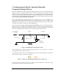
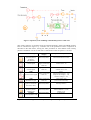
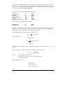
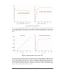
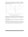
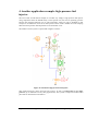
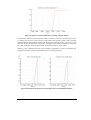
Thermal-Hydraulic Component Design Library
Version 4.2 – September 2004
®
Copyright  IMAGINE S.A. 1995-2004
AMESim® is the registered trademark of IMAGINE S.A.
AMESet® is the registered trademark of IMAGINE S.A.
ADAMS is a registered United States trademark of Mechanical Dynamics, Incorporated.
ADAMS/Solver and ADAMS/View are trademarks of Mechanical Dynamics, Incorporated.
MATLAB and SIMULINK are registered trademarks of the Math Works, Inc.
Netscape and Netscape Navigator are registered trademarks of Netscape Communications
Corporation in the United States and other countries. Netscape’s logos and Netscape product and
service names are also trademarks of Netscape Communications Corporation, which may be
registered in other countries.
PostScript is a trademark of Adobe Systems Inc.
UNIX is a registered trademark in the United States and other countries exclusively licensed by
X / Open Company Ltd.
Windows, Windows NT, Windows 2000 and Windows XP are registered trademarks of the
Microsoft Corporation.
X windows is a trademark of the Massachusetts Institute of Technology.
All other product names are trademarks or registered trademarks of their respective companies.
TABLE OF CONTENTS
1. Introduction..............................................................................................................1
2. Getting started with the Thermal-Hydraulic Component Design Library.........2
3. A new Thermal-Hydraulic properties submodel...................................................9
4. Another application example: high-pressure fuel injector.................................13
5. Formulation of equations and underlying assumptions .....................................22
5.1. PISTON SUBMODELS ..........................................................................................23
5.2. RESISTIVE COMPONENTS ..................................................................................23
5.3. CAPACITIVE COMPONENTS ...............................................................................24
5.4. FURTHER ASSUMPTIONS ...................................................................................26
5.5. OTHER IMPORTANT RULES ................................................................................26
References...................................................................................................................28
September 2004
Table of Contents
1/1
Using the Thermal-Hydraulic
Component Design Library
1. Introduction
The Thermal-Hydraulic Component Design Library (THCD) is used to construct a model of a
component from a collection of very basic blocks. This methodology is very efficient because it
enables you to go very deeply into the details of the components technology. For instance, all
types of hydraulic jacks, servo-valves, check valves can be modeled easily using this library.
It differs from the Hydraulic Component Design Library in that it allows you to study not only
the pressure levels and the flow rates distribution in the system but also the temperatures and the
enthalpy flow rates evolution in the system.
In special application cases for which pressure and temperature variations are wide (typically,
injection systems), this is of great importance. In this case it is no more realistic to work in
isothermal conditions and it becomes essential to consider the cross-coupling effects between
temperature and pressure and to take into account both on the calculation of the fluid thermalhydraulic properties. This is why special fluid properties are used in this library (note that these
properties are already used in the Thermal-Hydraulic Library).
For this reason, the THCD Library is fully compatible with the Thermal and Thermal-Hydraulic
Libraries. In addition, it contains the equivalent of all the submodels found in the HCD Library.
These submodels have been modified so as to account for thermal phenomena.
In this manual, several tutorial examples are presented to illustrate the use of this library and
finally a brief review of the theory and the assumptions used in this library is given.
We recommend you read and do the tutorial examples of the Thermal, Thermal-Hydraulic and
Hydraulic Component Design manuals before attempting the examples below.
September 2004
Using the Thermal-Hydraulic Component Design library
1/28
2. Getting started with the Thermal-Hydraulic
Component Design Library
The Thermal-Hydraulic Component Design library comprises a set of basic components from
which it is easy to model and observe the evolution of temperatures, pressures, mass and
enthalpy flow rates in hydraulic systems. Hence, we recommend you do the following example
as a first contact with the Thermal-Hydraulic Component Design library. If you did the tutorial
examples of the Thermal-Hydraulic library user’s guide, you will certainly recognize the system
shown in Erreur ! Source du renvoi introuvable..
In the Thermal-Hydraulic manual example, the pressure relief valve was modeled using
components from the Thermal-hydraulic library and the Signal library. This is a simple way of
modeling this pressure relief valve: we did not go into the details of the technology. That is what
we will do now, using the components of the THCD library.
The system shown in Erreur ! Source du renvoi introuvable. is part of a simplified injection
system. It consists of a pump that is feeding the injectors, a pressure relief valve and a tank in
which the flow rates coming from the pressure relief valve and the upstream part of the pump
are mixed. The distribution of mass flow rates is imposed as shown on the sketch.
200 L/hr
50 degC
100 L/hr
pump
injector
100 L/hr
25 L/hr
pressure
relief valve
75 L/hr
Figure 1: Simplified part of an injection system
In this example, the unit chosen for the volumetric flow rates is L/hr because it is one of the
commonly used units in injection systems.
To model this system, select the Thermal-Hydraulic and the Thermal-Hydraulic Component
Design libraries category icon shown in Figure 2.
Figure 2 : THCD and Thermal-Hydraulic libraries category icons
To produce the popup shown in Figure 3, select the Thermal-Hydraulic Component Design
library category icon shown in Figure 2(on the left).
September 2004
Using the Thermal-Hydraulic Component Design library
2/28
Figure 3: Components of the Thermal-Hydraulic Component Design Library
First, look at the components available in this library. Display the title for each component by
moving the pointer over the icons. When this is done, build the model of the check valve system
as shown in Figure 5.
In the first tutorial example of the Thermal-Hydraulic user’s guide, a simple pressure relief valve
is modelled (see Figure 4). It consists of a variable restriction. The upstream pressure is used to
control the opening of this restriction. It starts to open when the upstream pressure reaches 1000
bar. In this section, we will study the same system but this time we will model very accurately
the pressure relief valve using technological basic elements from the THCD library.
Figure 4: Simple model of a pressure relief valve
September 2004
Using the Thermal-Hydraulic Component Design library
3/28
Figure 5: Injection system including a THCD-built pressure relief valve
This model comprises 23 elements from the Thermal-hydraulic, Signal and THCD libraries.
Each is referenced in Figure 5 by a number. Fill in the parameters of these components as
described in the table below, leaving the other parameters at their default values. Finally,
perform a simulation over 50 seconds with a communication interval equal to 0.1 second.
Submodel name and type
0
1
2
TFFD1
thermal-hydraulic
properties
(polynomials)
CONS0
constant signal
CONS0
constant signal
Belongs to
category
Thermal-Hydraulic
Signal, control and
observers
Signal, control and
observers
Principal simulation parameters
filename to be used
$AME/libthh/data/diesel.data
constant value : 50
constant value : 100
piecewise linear signal
Signal, control and
observers
stage 1
output at start of stage 1 : 100
output at end of stage 1 : 100
duration of stage 1 : 50s
3, 6
GA00
submodel of a gain
Signal, control and
observers
value of gain :1/60
(convert L/hr into L/min)
4, 7
TFQT0
signal into volumetric
flow rate (L/min)
Thermal-Hydraulic
default parameters
UD00
5
8
9
TFPC1
thermal-hydraulic
adiabatic pipe
TFND01
thermal-hydraulic node
September 2004
Thermal-Hydraulic
Thermal-Hydraulic
temperature at port 1 : 50 degC
internal diameter : 12 mm
length : 0.4 m
no parameters
Using the Thermal-Hydraulic Component Design library
4/28
10
11, 17,
22
TF223
thermal- hydraulic
restriction
TFTK0
thermal-hydraulic tank
12, 16
13
14
F000
zero force source
THBAP026
thermal-hydraulic
poppet with conical
seat
THBAI21
mass with friction and
ideal end stops
15
THBAP16
thermal-hydraulic
piston with spring
18, 20
TFPC3
thermal-hydraulic
adiabatic pipe
TFPC2
thermal-hydraulic
adiabatic pipe
TFND03
Thermal-hydraulic
node
21
19
Thermal-Hydraulic
cross-sectional area : 0.018 mm2
default parameters
Thermal-Hydraulic
Mechanical
no parameters
Thermal-Hydraulic
Component Design
diameter of poppet : 5 mm
diameter of hole : 3.5 mm
diameter of rod : 0 mm
Thermal-Hydraulic
Component Design
mass: 0.01 kg
viscous friction: 40 [N/(m/s)]
lower disp. limit : 0 m
higher disp. limit : 0.001 m
piston diameter : 5 mm
Thermal-Hydraulicrod diameter : 0 mm
Component-Design
spring stiffness : 1000 N/mm
spring force at zero displacement :
pi*(3.5e-3)^2*1000e5/4N
chamber length at zero displacement :
1 mm
Thermal-Hydraulic
temperature at port 1 : 50 degC
Thermal-Hydraulic
temperature at port 2 : 50 degC
Thermal-Hydraulic
no parameters
The Thermal-Hydraulic Component Design library can be classified as shown below :
Thermal-Hydraulic
Component Design Library
Resistive Components
Mass flow rate
dm (kg/s)
Enthalpy flow
rates
dmh (W)
Transformer components
Convert a
pressure into a
force
Capacitive Components
Pressure
p (barA)
Temperature
T (degC)
Figure 6: Components classification in the THCD library
The resistive submodels can be described as steady-state submodels. A more accurate
description is they are instantaneous submodels. By this we mean that they are assumed to react
instantaneously to the temperatures and pressures applied to them so that they are always in an
equilibrium state.
September 2004
Using the Thermal-Hydraulic Component Design library
5/28
The capacitive submodels have two state variables: the temperature and the pressure that are
passed at ports. This means that each of these variables is defined by a differential equation.
These are very commonly used in Thermal-Hydraulic Component Design library systems and
we will describe them as transient submodels.
Six variables are exchanged at Thermal-Hydraulic ports:
Temperature
Pressure
Mass flow rate
Enthalpy flow rate
Volume
Derivative of the volume
T
p
dm
dmh
vol
dvol
[degC]
[barA]
[kg/s]
[W]
[cm3]
[L/min]
Two variables are exchanged at thermal ports:
Temperature
Heat flow rate
T
dh
[degC]
[W]
In order to reproduce the results obtained in the Thermal-Hydraulic manual tutorial example, we
design this pressure relief valve for 1000 bar. Thus, the spring force at zero displacement
corresponds to this pressure multiplied by the poppet seat section.
The seat diameter is 3.5 mm which implies a section of:
S seat =
The spring force F0 is:
π
4
× (3.5e − 3) 2
P =1000e5 Pa
F
P = 0 ⇒ F0 = P × S seat
S seat
F0 = 962.1 N
In order to avoid instabilities, we have to include an important viscous friction (Use Vf = 40
N/(m/s)).
The viscous friction coefficient is computed considering the relation below:
Vf = 2 × ξ × K × M
where:
K is the spring stiffness in N/m
M is the mass of the moving conical part of the poppet
ξ is the damping ratio
In this example, we chose
ξ = 20 %

 M = 0.01 kg
V = 40 N /(m / s )
 f
September 2004
Using the Thermal-Hydraulic Component Design library
6/28
From this, the spring stiffness can be deduced :
K = 1000 N / mm
Figure 7: Evolution of the temperature in the injection circuit
The main point of interest in this example is the evolution of the liquid temperature at the
pressure relief valve outlet and at the flow junction as shown in Figure 7 (components 13 and
20). There is a huge pressure drop in the pressure relief valve, which induces a dissipation of
energy by friction. This energy is transformed into heat that is transferred to the liquid. This
results in an increase in temperature at the relief valve outlet.
The liquid flows through the relief valve with an initial temperature of Ti = 50 degC. The
increase in temperature in the relief valve is approximately 56 degC. In Figure 7,we can see the
evolution of the mixing temperature. At this location in the circuit is a mixture of a 100 L/hr
volumetric flow rate which temperature is 50 degC and a 75 L/hr volumetric flow rate which
temperature is 106 degC. This results in a 175 L/hr volumetric flow rate in the tank with a
temperature of 74 degC. The transient and steady state behaviors of the system are strongly
related to the thermal properties of the liquid used for the simulation.
To observe this, display the pressure at the check valve inlet (see Figure 8(a)) (component
number 13) and the temperature at the same component outlet as shown in Figure 8 (b). You will
notice in this figure that these simulation results are compared to the simulation results obtained
with the simple pressure relief valve model shown in Figure 4.
September 2004
Using the Thermal-Hydraulic Component Design library
7/28
(a) simple pressure relief valve
(b) THCD relief valve
Figure 8: Results comparison
We can notice small differences in the results (Figure 8) due to the fact that the pressure relief
valve modeled with the THCD library is much more complex and includes more physical and
technological aspects in the system which in this case is more representative of a real relief
valve.
(a)
(b)
Figure 9: Dynamic behavior of the relief valve
In order to observe the dynamic behavior of the relief valve, set the parameters of the piecewise
linear signal (component 5) at 0 for the output at start of stage 1 and 200 for the output at end of
stage 1 with a duration of stage of 50 s. Perform a simulation and display the poppet lift (see
Figure 9(a)) and the pressure drop in the relief valve versus time as shown in Figure 9(b) above.
We can observe the cracking pressure at 1000 barA and the linear increase of the pressure drop
which is more representative of a real relief valve.
September 2004
Using the Thermal-Hydraulic Component Design library
8/28
3. A new Thermal-Hydraulic properties submodel
For most industrial applications where both pressure and temperature variations are important,
we recommend that you use TFFD2 submodel. This submodel uses polynomial functions to
evaluate the thermal-hydraulic properties of the liquid used for the simulation. The fluid
properties concerned are the density, the viscosity, the specific heat at constant pressure, the
thermal conductivity, the bulk modulus, the volumetric expansion coefficient and the specific
enthalpy. In this submodel, the order of the polynomial forms has been increased so that it
enables to reproduce very accurately the evolution of the fluid properties as a function of
pressure and temperature. In addition, this submodel accounts for cavitation phenomena. If you
need more information about the way these thermal-hydraulic properties are dealt with in the
THCD library, refer to the Thermal-Hydraulic Library user’s guide, in section “Advanced
Thermal-hydraulic properties”.
To test this advanced properties submodel, build the system shown in Figure 10. It comprises 5
elements from the Thermal-Hydraulic and the Signal libraries. Each element is referenced in
Figure 10 by a number. Fill in the parameters of these components as described in the table
below, leaving the other parameters at their default values.
Figure 10: Checking advanced thermal-hydraulic properties
Submodel name and type
TFFD2
0
thermal-hydraulic
advanced properties
with cavitation
UD00
1
Piecewise linear
signal
piecewise linear
signal
4
Thermal-hydraulic
TFPT0
conversion of a
signal into a
temperature and a
pressure
TFFPR
calculation of thermal
liquid properties
September 2004
Principal simulation parameters
filename :
$AME/libthh/data_advanced/
diesel80_rme20.data
stage1
Signal, control and
observers
output at start of stage 1 : 20
output at end of stage 1 : 20
duration of stage 1 : 1 sec
stage1
UD00
2
3
Belongs to category
Signal, control and
observers
output at start of stage 1 : 1
output at end of stage 1 : 2000
duration of stage 1 : 1 sec
Thermal-hydraulic
no parameters
Thermal-hydraulic
default parameters
Using the Thermal-Hydraulic Component Design library
9/28
Use the batch facility (in Tools menu, “Batch setup” option) to define four temperature values at
which the fluid properties will be calculated (20, 37, 80 and 120 [degC] ) and perform a
simulation over 1 second with a communication interval equal to 0.01 second. When this is
done, plot the density and the bulk modulus of the fluid versus pressure for these four
temperatures as shown in Figure 11.
Figure 11: Thermal properties of the liquid
From these results, it is easy to understand that variations in pressure and in temperature in a
thermal-hydraulic system have a great importance on the thermal-hydraulic properties of a fluid.
Indeed, if we consider a temperature variation from 20 to 120 degC at constant pressure (say
1000 barA), the density variation is almost equal to 60 kg/m3 (that is to say a 7% decrease of the
value of the density).
Similarly, if we consider a pressure variation from 1 to 2000 barA at constant temperature (say
20 degC), the density variation is almost equal to 70 kg/m3 (that is to say an increase of 8% of
the value of the density).
It follows that the cross-coupling effects between temperature and pressure have a strong impact
on the properties of the fluid. To observe this, display the evolution of all the properties
available for plotting in submodel TFFPR as shown in Figure 12. To do this, use the batch
facility to define five pressure values at which the fluid properties will be calculated (1, 500,
1000, 1500 and 2000 [barA]) and for each run, vary the temperature from 0 to 120 degC.
September 2004
Using the Thermal-Hydraulic Component Design library
10/28
Figure 12: Thermal-hydraulic properties of a special diesel fuel with respect to pressure
and temperature
In addition, the submodel TFFD2 takes into account cavitation phenomena. To show this,
change the parameters of component number 2 so as to vary the pressure from 0 to 1 barA.
Run the simulation using the same final time and communication interval as previously and
display the density and the bulk modulus of the fluid as a function of pressure for the four
temperatures defined above as shown in Figure 13.
Figure 13: Density and bulk modulus evolution in aeration and cavitation conditions
September 2004
Using the Thermal-Hydraulic Component Design library
11/28
To interpret these results, it is important to know that the saturation pressure is equal to 2000
barA. This means that below this pressure, dissolved air and gas are coexisting in the fluid.
Before pressure decreases to 0.5 barA, the dissolved air turns into gas into the liquid. Therefore,
the fluid density and the bulk modulus are decreasing. When the liquid begins to vaporize, there
is a sudden decrease of the bulk modulus and the density, the air dissolved is totally transformed
into gas. At this stage, it is necessary to do a zoom on the interesting region of the graphs which
is lying between 0 and 0.5 barA as shown in Figure 14.
pvaph
pvapl
Figure 14: Influence of liquid vaporization on the fluid density and bulk modulus
When the pressure reaches pvaph = 0.5 barA, the liquid starts to vaporize and it is totally
vaporized when the pressure has reached pvapl = 0.4 barA. These two pressures correspond
respectively to the high saturated vapor pressure and the low saturated vapor pressure of the
liquid. These two pressures are parameters of submodel TFFD2 and can be changed.
Finally, when the pressure value is in the range 0 to 0.4 barA, it is considered that almost all the
liquid has turned into vapor and as a result, a polytropic law is used to describe the properties of
the gas.
Please refer to Technical Bulletin N°117 “AMESim Standard Fluid Properties” for full details
on the cavitation model used in submodel TFFD2.
September 2004
Using the Thermal-Hydraulic Component Design library
12/28
4. Another application example: high-pressure fuel
injector
The aim of this second tutorial example is to model very simply a high pressure fuel injector
using components from the THCD library. In this special case, the level of operating pressure
and the fast transient behaviour are of great importance. What we want to highlight in this
example is the difference observed on the injected volume results whether the cross-coupling
effects between pressure and temperature are accounted for or not.
The model of such a system is represented in Figure 15 below:
Figure 15: Model of a high pressure fuel injector
This model represents a basic electronic unit injector. Its aim is to inject fuel at very highpressure (up to 2000 bar for heavy-duty applications). This system is composed of three main
parts that are described in what follows:
September 2004
Using the Thermal-Hydraulic Component Design library
13/28
Part A: The control valve
Part B: The plunger
Part C: the needle
The operating principle of such a system is the following: a cam-controlled plunger (part B)
compresses a small volume (chamber 11) filled with fuel. When the control valve is open, all the
fuel flows to the low-pressure circuit (tank 6). When the control valve closes the pressure rises
very quickly and reaches the needle cracking pressure (modeled with components 13, 14, 15).
The injection starts. When the control valve opens again, the pressure decrease is very fast and
the injection is stopped.
The complete model comprises twenty components from the Thermal, Thermal-Hydraulic,
Signal and THCD libraries. Each is referenced in Figure 15 by a number. Fill in the parameters
of these components as described in the table below, leaving the other parameters at their default
values. When this is done, run a simulation for 0.015 seconds with a communication interval of
0.0001 seconds.
September 2004
Using the Thermal-Hydraulic Component Design library
14/28
Submodel name and type
Belongs to
category
Principal simulation parameters
time at which duty cycle starts : 5e-3 sec
0
UD00
piecewise linear signal
1
UD00
piecewise linear signal
2
3
4
5
6, 8a, 8b
7
9
Signal,
control and
observers
INTO
submodel of integrator
SSINK
submodel for plugging a
signal port
TFFD2
thermal-hydraulic
advanced properties with
cavitation
TFVR0
thermal-hydraulic variable
restriction,
dm = f (cqmax, lamc)
TFTK0
thermal-hydraulic tank
TFVF0
thermal-hydraulic
volumetric flow rate sensor
VELC02
conversion of a signal to a
velocity in m/s and a
displacement in m
September 2004
Signal,
control and
observers
stage1
output at start of stage 1 : 0
output at end of stage 1 : 2.5
duration of stage 1 : 3e-3 sec
stage2
output at start of stage 2 : 2.5
output at end of stage 2 : 2.5
duration of stage 2 : 4e-3 sec
stage3
output at start of stage 3 : 2.5
output at end of stage 3 : 0
duration of stage 3 : 3e-3 sec
stage1
output at start of stage 1 : 1
output at end of stage 1 : 1
duration of stage 1 : 9e-3 sec
stage 2
output at start of stage 2 : 0
output at end of stage 2 : 0
duration of stage 2 : 2e-3 sec
stage 3
output at start of stage 3 : 1
output at end of stage 3 : 1
duration of stage 3 : 1e6 sec
Control
value of gain : 1e6/60
Control
No parameters
Thermalhydraulic
filename :
$AME/libthh/data_advanced/diesel80_rme20.data
cross sectional area : 4*pi mm2
Thermalhydraulic
Thermalhydraulic
tank pressure : 1 barA
tank temperature : 40 degC
Thermalhydraulic
default parameters
Mechanical
default parameters
Using the Thermal-Hydraulic Component Design library
15/28
10, 11, 12
F000
zero force source
Mechanical
no parameters
THBAP026
thermal-hydraulic poppet
with conical seat
ThermalHydraulic
Component
Design
diameter of poppet : 5 mm
diameter of hole : 3 mm
diameter of rod : 0 mm
THBAI21
mass with friction and ideal
end stops
ThermalHydraulic
Component
Design
mass : 0.01 kg
viscous friction : 40 [N/(m/s)]
lower disp. limit : 0 m
higher disp. limit : 5e-5 m
THBAP16
thermal-hydraulic piston
with spring
ThermalHydraulic
Component
Design
13
14
15
16
THBAP12
piston
17
18
19
20
ThermalHydraulic
Component
Design
ThermalTHBHC12
thermal-hydraulic chamber
Hydraulic
with heat transfer
Component
Design
THCDC0
contact conductive
Thermal
exchange
THTS1
constant temperature source
TFN221
thermal hydraulic node
piston diameter : 5 mm
rod diameter : 0 mm
spring stiffness : 1000 N/mm
spring force at zero displacement :
pi*(3e-3)^2*300e5/4N
chamber length at zero displacement : 1 mm
piston diameter : 10 mm
rod diameter : 0 mm
chamber length at zero displ. : 17 mm
pressure at port 1 : 1 barA
temperature at port 1 : 40 degC
dead volume : 1.5 cm3
thermal contact conductance: 1e10 W/m2/degC
contact surface: 1e10 mm2
Thermal
temperature at port 1 : 40 degC
Thermalhydraulic
no parameters
If you look carefully at the model shown in Figure 16, you can notice that the fluid in the
hydraulic chamber can exchange heat with the outside. At this stage an explanation is necessary.
First consider Figure 16 below:
Figure 16: Thermal-hydraulic chamber with heat exchanged
September 2004
Using the Thermal-Hydraulic Component Design library
16/28
The thermal-hydraulic chamber (component 17) comprises 3 thermal-hydraulic ports and 1
thermal port. The thermal port is used to model a heat exchange between the liquid in the
chamber and the outside. The hydraulic chamber supplies the temperature of the fluid at the
thermal port, the temperature source (component number 19) constitutes the ambient air
temperature and component 18 is used to calculate the heat exchange between the chamber and
the outside.
In component 18, if the parameters supplied imply a heat exchange between the fluid and the
outside which is very high, the temperature of the liquid in the chamber will be kept to 40 degC.
As a result, all the transformation in the hydraulic chamber will be isothermal.
Conversely, if the parameters supplied in component 18 imply a heat exchange between the fluid
and the outside which tends to zero (minimum values for the thermal contact conductance and
the contact surface), it will be possible to study the temperature evolution of the fluid in the
hydraulic chamber.
Therefore, setting the parameters of component 18 at very high values will be used to mask the
cross-coupling effects between pressure and temperature whereas setting these parameters at
their minimum values will be used to study the influence of the cross-coupling effect between
temperature and pressure on the results. Doing this will highlight the result differences on the
injected volume.
Display the velocity of the piston (component 0), the pressure in the chamber (component 17),
the input signal on the control valve (component 1) and the poppet lift (component 13) as shown
in Figure 17 below:
Figure 17: Control variables and behaviour of the system
September 2004
Using the Thermal-Hydraulic Component Design library
17/28
In this system, the velocity of the piston is imposed as shown in Figure 17. As the piston starts to
move, the fluid is compressed in the chamber due to chamber length variations. At the beginning
of the simulation, the control valve is fully opened. As a result the flow coming from the
chamber and resulting from the displacement of the piston passes totally through the control
valve (low pressure circuit). At time t = 0.009 seconds, the control valve is closed
instantaneously (look at the curve in Figure 17 describing the input signal which is used to
control the opening and the closing of the control valve) and as a result, the pressure in the
hydraulic chamber suddenly increases. When this pressure reaches and overcomes the needle
cracking pressure, the injection starts. When the control valve opens again, the pressure in the
chamber suddenly decreases and becomes smaller than the needle cracking pressure. At this
stage, the injection is interrupted and the fuel flows to the low pressure circuit.
By setting very high values for the parameters of component 18, we model a chamber with a
heat exchange with the outside which is infinite. As a result, the temperature in the chamber
remains constant and equal to 40 degC.
Display the evolution of the pressure and the temperature in the chamber with the high values
for the parameters of component 8 (as specified in the previous table) as shown in Figure 18
below:
Figure 18: Evolution of the pressure and the temperature in the chamber (infinite heat
exchange with the outside)
In this case, the pressure in the chamber increases up to 1975 barA and the temperature in the
chamber remains constant and is equal to 40 degC.
Display now the results for the injected volume as shown in Figure 19 below. This information
is given by the output of component number 2.
September 2004
Using the Thermal-Hydraulic Component Design library
18/28
.
Figure 19: Injected volume (infinite heat exchange with the outside)
In isothermal conditions, the total injected volume is equal to 223 mm**3. At this stage, we want
to compare the previous results (pressure, temperature and injected volume) with the results
obtained when the heat exchange between the fluid and the chamber tends to zero, that is to say
when the chamber is adiabatic. To model this, change the values of the parameters of component
18 to their minimum values (for the thermal conductance and the contact surface).
Perform a new simulation with the same simulation parameters as before and display the
temperature and the pressure in the chamber as shown in Figure 20 below.
Figure 20: Evolution of the pressure and temperature in the adiabatic chamber
September 2004
Using the Thermal-Hydraulic Component Design library
19/28
On the graph of Figure 20, it is possible to notice that the increase in temperature is strongly
related to the increase in pressure. Indeed, the temperature evolution follows the pressure
evolution. During the compression of the hydraulic chamber, the temperature, which was
originally equal to 40 degC, reaches 67 degC when the pressure in the chamber is at its
maximum. This illustrates clearly the cross-coupling effect between temperature and pressure. In
addition, you can compare the results obtained for the pressure with infinite heat exchange and
with zero heat exchange as shown in Figure 21.
Figure 21: Comparison of pressure results
Figure 21 shows that the level of pressure reached in the case of an adiabatic chamber is equal to
2212 barA whereas the level of pressure reached in the case of an infinite heat exchange
between the chamber and the outside is equal to 1975 barA. There is a difference of 12%
between these two values.
We can wonder if this will have an impact on the results obtained for the injected volume.
Display on the same graph as shown in Figure 22 the evolution of the injected volume in the
case of an adiabatic chamber and in the case of an infinite heat exchange between the fluid in the
chamber and the outside.
September 2004
Using the Thermal-Hydraulic Component Design library
20/28
Figure 22: Comparison on the injected volume (adiabatic chamber and infinite heat
exchange)
In the adiabatic case, the total injected volume is higher than in the case of an infinite heat
exchange (the temperature in the chamber remains constant). Indeed, the total injected volume is
equal to 240.5 mm3 in the adiabatic case and it is equal to 223 mm3 when the temperature
remains constant in the chamber. This means that neglecting the evolution of the temperature
due to the compression of the volume can imply errors on the injected volume calculated that are
close to 8 % !!
This is easily conceivable because the evolution of the pressure and the temperature in the
chamber has a strong influence on the thermal-hydraulic properties of the injected fluid (this is
what was highlighted in a previous section when the evolution of the fluid thermal-hydraulic
properties was plotted).
September 2004
Using the Thermal-Hydraulic Component Design library
21/28
5. Formulation of equations and underlying assumptions
The Thermal Hydraulic Component Design library comprises four kinds of elements that are:
• mass submodels (inertial components)
• piston submodels (transformer components)
• valve submodels (resistive components)
• chamber submodels (capacitive components)
The first two rows of components are used for absolute motion. The three last components are
purely ydraulic components with thermal effects. The other components are used for relative
motion. With the relative motion models, both the internal and external elements of the
submodels are capable of motion. With the absolute motion models, the body is considered fixed
in space. We will concentrate on the absolute motion icons.
September 2004
Using the Thermal-Hydraulic Component Design library
22/28
5.1. Piston submodels
The active area on which pressure acts is very important in hydraulic systems. The one
hydraulic port submodels have their mass and enthalpy flow rate equal to 0. These components
have to be connected to a thermal-hydraulic chamber to exchange the volume variation and its
derivative information (which is now used to compute pressure and temperature). In the one
hydraulic port submodels, we will find only pistons (with or without springs).
5.2. Resistive components
These submodels are used to compute the mass flow rate using Bernoulli’s equation:
•
dm = ρ .cq .A
2.∆p
ρ
Cq is the flow coefficient,
A is the flow area calculated from the geometry of the component,
∆p is the pressure drop in the component,
ρ is the density computed at a working temperature and pressure.
The enthalpy flow rate in the component is computed as follows:
[null]
[m2]
[PaA]
[kg/m3]
dmh = dm × h
where dm is the mass flow rate through the resistive component and h is the specific
enthalpy of the fluid.
The mass and enthalpy flow rates are computed at port 2 and are duplicated at port 1 with
reversed sign. Every THCD valve is an adiabatic component meaning that the energy dissipated
in it is completely transferred to the liquid. Nothing is exchanged with its surroundings.
The submodel shown above is used for the calculation of hydraulic leakage and corresponding
viscous friction forces. It is also a resistive component in which the flow path is assumed to be
in the annular area between the cylindrical spool or piston and a cylindrical sleeve. The length of
this clearance flow path is assumed constant.
The leakage is directly proportional to the differential pressure, the diameter and the cube of the
clearance and inversely proportional to absolute viscosity and contact length.
September 2004
Using the Thermal-Hydraulic Component Design library
23/28
5.3. Capacitive components
The two icons indicated as ‘Ch’ on the figure are capacitive components, that is to say that they
compute pressure and temperature from their derivatives with respect to time. Similar to the
resistive components, six variables are exchanged at each port with the difference that thermalhydraulic chambers receive mass flow rate, enthalpy flow rate, volume and its derivative and
provide pressure and temperature.
The mass of liquid in the volume is given by:
m = ρ ×V
(1)
The continuity equation for the one-dimensional flow gives:
•
dm
= ∑ mi , i represents the number of inputs of the control volume(2)
dt
i
It is possible, from equation (1) and (2), to formulate the continuity equation in terms of the
density derivative as follows:
dm
dV
−ρ
dρ
dt
= dt
dt
V
(3)
The density being a thermodynamic property of the liquid, it is a function of pressure and
temperature:
ρ = ρ( p,T )
(4)
By differentiating with respect to temperature and pressure, equation (4) leads to:
 ∂ρ 
 ∂ρ 
dρ =   ⋅ dp +   ⋅ dT
 ∂T  p
 ∂p  T
(5)
From this equation, it is possible to write the continuity equation in terms of the pressure
derivative as follows:
dp =
September 2004
1
 ∂ρ 
 
 ∂p  T


 ∂ρ 
 ⋅ dT 
dρ − 
 ∂T  p


Using the Thermal-Hydraulic Component Design library
(6)
24/28
Using the definition of the liquid properties and more particularly the isothermal Bulk modulus
(βT ) and the volumetric expansion coefficient, the pressure derivative with respect to time is
given by:
dp
= βT
dt
 1 dρ
dT 
⋅  . + αp ⋅
dt 
 ρ dt
(7)
using equation (3), (6) leads to:
dp
= βT
dt
 1
⋅
 ρ.V
dV 
dT 
 dm
(8)
.
−ρ
 + αp ⋅
dt 
dt 
 dt
where:
β T ( p, T ) =
ρ
 ∂ρ 
is the isothermal fluid bulk modulus
[PaA]
is the volumetric expansion coefficient.
[1/K]
 
 ∂p  T
α p ( p,T ) = −
1  ∂ρ 
⋅

ρ  ∂T  p
The temperature is a state variable and is computed from the energy conservation assumption.
The first equation describes the relationship between the specific internal energy and the specific
enthalpy of the liquid:
u =h−
p
ρ
(9)
where u is the specific internal energy [W], h is the specific enthalpy [W], p is the pressure
[PaA]and ρ is the density of the liquid [kg/m3]. The energy in the control volume is given by:
E = m⋅u +
mV 2
+ mgz
2
(10)
The three terms in equation (10) represent respectively the internal energy, the kinetic energy
and the potential energy.
We modify equation (10) introducing the second assumption: the kinetic and potential
energies in the control volume are neglected. This leads to:
E = mu
(11)
The derivative of the specific enthalpy can be written as follows:
dT (1 − Tα p ) dp
dh
= cp
+
dt
ρ
dt
dt
September 2004
Using the Thermal-Hydraulic Component Design library
(12)
25/28
Differentiating and combining equations (9), (11) and (12) leads to the following relation:
m.c p .
mα p T dp
dT
= dmhi − dmho + Q& +
− dm × h
ρ dt
dt
(13)
where m is the mass of liquid in the volume, cp is the specific heat of the liquid at constant
pressure, dmhi is the incoming enthalpy flow rate, dmho is the outgoing enthalpy flow rate, Q& is
the heat flow rate exchanged with the outside, V is the volume, dm is the mass flow rate through
the volume, α is the volumetric expansion coefficient, ρ is the fluid density and h is the specific
enthalpy.
Finally, the temperature derivative with respect to time is given by:
dT dmhi − dmho − dm × h + Q&
Tα dp
=
+
.
dt
m.c p
ρ .c p dt
(14)
Equation (14) is the complete energy equation represented by the temperature derivative with
respect to time. The pressure derivative term in this equation shows the cross-coupling effect
with the continuity equation (8) represented by the pressure derivative with respect to time.
5.4. Further assumptions
Concerning the thermal aspects in the components of the thermal-hydraulic library, the
following assumptions are made :
•
•
•
•
•
•
the flow is one dimensional,
the properties of the liquid are homogeneous in the volumes,
aeration and cavitation phenomena are taken into account when using submodel
TFFD2,
in the liquids, heat transfers by radiation or conduction are neglected,
the displayed temperatures are total temperatures,
components of the THCD library enable you to model multi-fluid systems.
5.5. Other important rules
• The THCD library deals with liquids only.
• It is better if the user builds the system slowly and run a simulation after each portion of
circuit is added. This normally leads to a better understanding of the system and the results. It is
also less likely that the setting of parameters will be forgotten. The user will have to be very
careful when running multi-liquid simulations: the indices of thermal hydraulic fluid must be
adjusted in the corresponding submodels.
• Files of thermal liquid properties are available in the $AME/libthh/data (for use with submodel
TFFD1) and the $AME/libthh/data_advanced (for use with submodel TFFD2) directories.
September 2004
Using the Thermal-Hydraulic Component Design library
26/28
• This version of the THCD library includes about 100 submodels. Full documentation of these
submodel is available in HTML format or, more briefly, directly in AMESim, in the description
of each submodel.
• The AMESim thermal-hydraulic library can be coupled with the thermal library to study
thermal interactions between liquids and solids. Really in the THCD library, thermal ports have
been added to hydraulic components (Figure 23).
Thermal component
Thermal ports
THCD component
Figure 23: coupling Thermal and THCD components
September 2004
Using the Thermal-Hydraulic Component Design library
27/28
References
[Ref. 1]
INCROPERA F.P., DEWITT D.P., "Fundamentals of Heat and Mass
Transfer", Fourth Edition, John Wiley & Sons, 1996.
[Ref. 2]
EYGLUNENT B., "Thermique théorique et pratique à l'usage de l'ingénieur",
Editions Hermès, 1994.
[Ref. 3]
BOREL L., "Thermodynamique et énergétique", Vol 1 troisième édition,
Editions Presses polytechniques romandes, 1991.
[Ref. 4]
MILLER D.S., "Internal Flow systems", 2nd Edition, Amazon Technology,
1989.
[Ref. 5]
FAISANDIER J., "Mécanismes oléo-hydrauliques", Editions Dunod, 1987.
[Ref. 6]
IMAGINE S.A., "Hydraulic Component Design user manual", 2000.
[Ref. 7]
IMAGINE S.A, "Thermal-Hydraulic Library user manual", 2000.
September 2004
Using the Thermal-Hydraulic Component Design library
28/28
Reporting Bugs and using the Hotline
Service
AMESim is a large piece of software containing many hundreds of thousands of lines of
code. With software of this size it is inevitable that it contains some bugs. Naturally we
hope you do not encounter any of these but if you use AMESim extensively at some
stage, sooner or later, you may find a problem.
Bugs may occur in the pre- and post-processing facilities of AMESim, AMESet or in one
of the interfaces with other software. Usually it is quite clear when you have encountered
a bug of this type.
Bugs can also occur when running a simulation of a model. Unfortunately it is not
possible to say that, for any model, it is always possible to run a simulation. The
integrators used in AMESim are robust but no integrator can claim to be perfectly
reliable. From the view point of an integrator, models vary enormously in their difficulty.
Usually when there is a problem it is because the equations being solved are badly
conditioned. This means that the solution is ill-defined. It is possible to write down sets of
equations that have no solution. It such circumstances it is not surprising that the
integrator is unsuccessful. Other sets of equations have very clearly defined solutions.
Between these extremes there is a whole spectrum of problems. Some of these will be the
marginal problems for the integrator.
If computers were able to do exact arithmetic with real numbers, these marginal problems
would not create any difficulties. Unfortunately computers do real arithmetic to a limited
accuracy and hence there will be times when the integrator will be forced to give up.
Simulation is a skill which has to be learnt slowly. An experienced person will be aware
that certain situations can create difficulties. Thus very small hydraulic volumes and very
small masses subject to large forces can cause problems. The State count facility can be
useful in identifying the cause of a slow simulation. An eigenvalue analysis can also be
useful.
The author remembers spending many hours trying to understand why a simulation failed.
Eventually he discovered that he had mistyped a parameter. A hydraulic motor size had
been entered making the unit about as big as an ocean liner! When this parameter was
corrected, the simulation ran fine.
In follows that you must spend some time investigating why a simulation runs slowly or
fails completely. However, it is possible that you have discovered a bug in an AMESim
submodel or utility. If this is the case, we would like to know about it. By reporting
problems you can help us make the product better.
On the next page is a form. When you wish to report a bug please photocopy this form
and fill the copy. Even if you telephone us, having the filled form in front of you means
you have the information we need.
To report the bug you have three options:
fax the form
reproduce the same information as an email
telephone the details
Use the fax number, telephone number or email address of your local distributor.
HOTLINE REPORT
Creation date:
Created by:
Company:
Contact:
Keywords (at least one):
Problem type:
! Bug
! Improvement
! Other
Summary:
Description:
Involved operating system(s):
! All
! Unix (all)
! PC (all)
! HP
! Windows 2000
! IBM
! Windows NT
! SGI
! Windows XP
! SUN
! Linux
! Other:
! Other:
Involved software version(s):
! All
! AMESim (all)
! AMERun (all)
! AMESet (all)
! AMECustom (all)
! AMESim 4.0
! AMERun 4.0
! AMESet 4.0
! AMECustom 4.0
! AMESim 4.0.1 ! AMERun 4.0.1 ! AMESet 4.0.1
! AMECustom 4.0.1
! AMESim 4.0.2 ! AMERun 4.0.2 ! AMESet 4.0.2
! AMECustom 4.0.2
! AMESim 4.0.3 ! AMERun 4.0.3 ! AMESet 4.0.3
! AMECustom 4.0.3
! AMESim 4.1
! AMECustom 4.1
! AMERun 4.1
! AMESet 4.1
Web Site
http://www.amesim.com
FRANCE - ITALY - SPAIN –
PORTUGAL - BENELUX SCANDINAVIA
S.A.
5, rue Brison
42300 ROANNE - FRANCE
Tel. : 04-77-23-60-30
Tel. : (33) 4-77-23-60-37
Fax : (33) 4-77-23-60-31
E.Mail : [email protected]
CHINA
China
Room. 109
Jinyan Building (Business), N. 3800 Chunshen Road,
Shanghai 201100
CHINA (PRC)
E-mail: [email protected]
United Right Technology
UK
U.K.
Park Farm Technology Centre
Kirtlington, Oxfordshire
OX5 3JQ
ENGLAND
Tel: +44 (0) 1869 351 994
Fax: +44 (0) 1869 351 302
E-mail: [email protected]
USA - CANADA - MEXICO
Software, Inc.
44191 Plymouth Oak Blvd – Suite 900
PLYMOUTH (MI) 48170 - USA
Tel. : (1) 734-207-5557
Fax : (1) 734-207-0117
E.Mail : [email protected]
GERMANY - AUSTRIASWITZERLAND
Software GmbH
Elsenheimerstr. 15
D - 80687 München - DEUTSCHLAND
Tel: +49 89 / 548495-35
Fax: +49 89 / 548495-11
E.Mail : [email protected]
Room 716-717
North Office Tower Beijing, New World Center
No.3-B Chong Wen MenWai dajie,
Postal Code: 100062, BEIJING, P.R CHINA
Tel: (86) 10-67082450(52)(53)(54)
Fax: (86) 10-67082449
E.Mail: [email protected]
SOUTH KOREA
SHINHO Systems Co., Ltd.
#702
Ssyongyong IT Twin Tower
442-5, Sangdaewon-dong
Jungwon-gu
Seongnam-si
Gyeonggi
South Korea <462-723 >
Tel. : 82-31-608-0434
Fax : 82-31-608-0439
E.Mail : [email protected]
BRAZIL
KEOHPS
CELTA – Parc Tec ALFA
Rod. SC 401-km 01 – CEP 88030-000
FLORIANOPOLIS – SC BRAZIL
Tel. : (55) 48 239 – 2281
Fax : (55) 48 239 – 2282
E.Mail : [email protected]
HUNGARY
JAPAN
Japan KK
SATOKURA AKEBONOBASHI Bldg. 2F
SHINJUKU KU, SUMIYOSHI MACHI, 1-19
TOKYO 162-0065 - JAPAN
Tel. : 81 (0) 3 3351 9691
Fax : 81 (0) 3 3351 9692
E.Mail : [email protected]
Budapest University of
Technology & Economics
Department of Fluid Mechanics
H-1111 BUDAPEST, Bertalan L. U. 4- 6 HUNGARY
Tel. : (36) 1 463 4072 / 463 2464
Fax : (36) 1 463 3464
E.Mail : [email protected]