Download Dynamic Link Library Solver User`s Guide

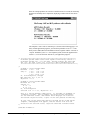
Dynamic Link Library • Version 3.5
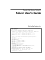
Solver User's Guide
By Frontline Systems, Inc.
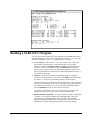
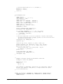
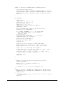
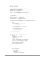
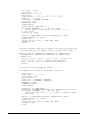
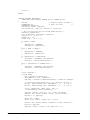
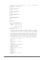
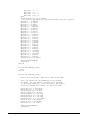
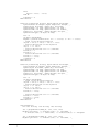
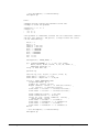
#include "frontmip.h"
#include "frontkey.h"
#include <stdio.h>
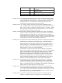
INTARG _CC FuncEval (HPROBLEM lp, INTARG numcols, INTARG numrows,
LPREALARG objval, LPREALARG rhs, LPREALARG var, INTARG varone, INTARG vartwo)
{
objval[0] = var[0] * var[0] + var[1] * var[1]; /* objective */
lhs[0] = var[0] + var[1]; /* constraint left hand side: = 1.0 */
lhs[1] = var[0] * var[1]; /* constraint left hand side: >= 0.0 */
return 0;
}
int main() /* Solve example constrained nonlinear optimization problem */
{
double obj[2];
double rhs[2] = { 1.0, 0.0 };
char sense[2] = "EG";
double matval[4];
double lb[] = { -INFBOUND, -INFBOUND };
double ub[] = { +INFBOUND, +INFBOUND };
long stat, i;
double x[2] = {0.0, 0.0 };
double objval, piout[2], slack[2];
HPROBLEM lp;
printf("Example NLP problem\n");
lp = loadnlp (PROBNAME, 2, 2, 1, obj, rhs, sense,
NULL, NULL, NULL, matval, x, lb, ub, NULL, 4, FuncEval, NULL);
optimize (lp);
solution (lp, &stat, &objval, x, piout, slack, NULL);
printf("Status = %ld Objective = %g\n", stat, objval);
printf("Final values: x[0] = %7g x[1] = %7g\n", x[0], x[1]);
for (i = 0; i <= 1; i++)
printf("slack[%ld] = %7g dual value[%ld] = %7g\n",
i, slack[i], i, piout[i]);
return 0;
}
Copyright
Software copyright  1991-1999 by Frontline Systems, Inc.
Portions copyright  1989 by Optimal Methods, Inc.
Portions copyright  1994 by Software Engines.
User Manual copyright  1999 by Frontline Systems, Inc.
Neither the Software nor this User Manual may be copied, photocopied, reproduced, translated, or reduced to any
electronic medium or machine-readable form without the express written consent of Frontline Systems, Inc., except as
permitted by the Software License agreement on the next page.
Trademarks
Microsoft, Windows, Visual C++, and Visual Basic are trademarks of Microsoft Corporation.
Delphi is a trademark of Borland International.
Pentium is a trademark of Intel Corporation.
How to Order
Contact Frontline Systems, Inc., P.O. Box 4288, Incline Village, NV 89450.
Tel (775) 831-0300 • Fax (775) 831-0314 • Email [email protected] • Web http://www.frontsys.com
SOFTWARE LICENSE
Unless other license terms are specified in a written license agreement between Frontline Systems, Inc. (“Frontline”) and
you or your company or institution, Frontline grants only a license to use one copy of the enclosed computer program
(the “Software”) on a single computer by one person. The Software is protected by United States copyright laws and
international treaty provisions. Therefore, you must treat the Software just like any other copyrighted material, except
that: You may store the Software on a hard disk or network server, provided that only one person uses the Software on
one computer at a time, and you may make one copy of the Software solely for backup purposes. You may not rent or
lease the Software, but you may transfer it on a permanent basis if the person receiving it agrees to the terms of this
license. This license agreement is governed by the laws of the State of Nevada.
LIMITED WARRANTY
THE SOFTWARE IS PROVIDED “AS IS” WITHOUT WARRANTY OF ANY KIND. THE ENTIRE RISK AS TO
THE RESULTS AND PERFORMANCE OF THE SOFTWARE IS ASSUMED BY YOU. Frontline warrants only that
the diskette(s) on which the Software is distributed and the accompanying written documentation (collectively, the
“Media”) is free from defects in materials and workmanship under normal use and service for a period of ninety (90) days
after purchase, and any implied warranties on the Media are also limited to ninety (90) days. SOME STATES DO NOT
ALLOW LIMITATIONS ON THE DURATION OF AN IMPLIED WARRANTY, SO THE ABOVE LIMITATION
MAY NOT APPLY TO YOU. Frontline's entire liability and your exclusive remedy as to the Media shall be, at
Frontline's option, either (i) return of the purchase price or (ii) replacement of the Media that does not meet Frontline's
limited warranty. You may return any defective Media under warranty to Frontline or to your authorized dealer, either of
which will serve as a service and repair facility.
EXCEPT AS PROVIDED ABOVE, FRONTLINE DISCLAIMS ALL WARRANTIES, EITHER EXPRESS OR
IMPLIED, INCLUDING BUT NOT LIMITED TO IMPLIED WARRANTIES OF MERCHANTABILITY AND
FITNESS FOR A PARTICULAR PURPOSE, WITH RESPECT TO THE SOFTWARE AND THE MEDIA. THIS
WARRANTY GIVES YOU SPECIFIC RIGHTS, AND YOU MAY HAVE OTHER RIGHTS WHICH VARY FROM
STATE TO STATE.
IN NO EVENT SHALL FRONTLINE BE LIABLE FOR ANY DAMAGES WHATSOEVER (INCLUDING
WITHOUT LIMITATION DAMAGES FOR LOSS OF BUSINESS PROFITS, BUSINESS INTERRUPTION, LOSS
OF BUSINESS INFORMATION, AND THE LIKE) ARISING OUT OF THE USE OR INABILITY TO USE THE
SOFTWARE OR THE MEDIA, EVEN IF FRONTLINE HAS BEEN ADVISED OF THE POSSIBILITY OF SUCH
DAMAGES. BECAUSE SOME STATES DO NOT ALLOW THE EXCLUSION OR LIMITATION OF LIABILITY
FOR INCIDENTAL OR CONSEQUENTIAL DAMAGES, THE ABOVE LIMITATION MAY NOT APPLY TO YOU.
In states which allow the limitation but not the exclusion of such liability, Frontline's liability to you for damages of any
kind is limited to the price of one copy of the Software and Media.
U.S. GOVERNMENT RESTRICTED RIGHTS
The Software and Media are provided with RESTRICTED RIGHTS. Use, duplication or disclosure by the Government
is subject to restrictions as set forth in subdivision (b)(3)(ii) of The Rights in Technical Data and Computer Software
clause at 252.227-7013. Contractor/manufacturer is Frontline Systems, Inc., P.O. Box 4288, Incline Village, NV 89450.
THANK YOU FOR YOUR INTEREST IN FRONTLINE SYSTEMS, INC.
Contents
Introduction
5
The Solver Dynamic Link Libraries........................................................................................... 5
The Small-Scale Solver DLL..................................................................................................... 5
The Large-Scale Solver DLL..................................................................................................... 6
Which Solver DLL Should You Use?........................................................................................ 7
Linear Solver ............................................................................................................... 7
Quadratic Solver.......................................................................................................... 8
Nonlinear Solver.......................................................................................................... 8
Nonsmooth (Evolutionary) Solver............................................................................... 9
Solving Mixed-Integer Problems................................................................................. 9
16-Bit Versus 32-Bit Versions..................................................................................... 9
What’s New in Version 3.5...................................................................................................... 10
Evolutionary Solver ................................................................................................... 10
Multi-Threaded Applications..................................................................................... 10
Use-Based Licensing ................................................................................................. 10
Problems in Algebraic Notation ................................................................................ 11
How to Use This Guide............................................................................................................ 11
Installation
15
Running the Installation Program ............................................................................................ 15
Copying Disk Files Manually .................................................................................................. 15
Directory Paths ........................................................................................................................ 16
Licensing the Solver DLL........................................................................................................ 17
Registry Entries for Use-Based Licensing ............................................................................... 17
Designing Your Application
19
Calling the Solver DLL............................................................................................................ 19
Solving Linear and Quadratic Problems .................................................................................. 19
Solving Nonlinear Problems .................................................................................................... 20
Solving Nonsmooth Problems.................................................................................................. 21
Genetic and Evolutionary Algorithms ....................................................................... 21
Problems in Algebraic Notation............................................................................................... 22
Using Other Solver DLL Routines........................................................................................... 23
Determining Linearity Automatically ...................................................................................... 23
Supplying a Jacobian Matrix.................................................................................................... 24
Diagnosing Infeasible Problems .............................................................................................. 24
Solution Properties of Quadratic Problems.............................................................................. 25
Passing Dense and Sparse Array Arguments ........................................................................... 26
Arrays and Callback Functions in Visual Basic ....................................................................... 28
Using the Solver DLL in Multi-Threaded Applications........................................................... 29
Use-Based Licensing ................................................................................................. 29
Dynamic Link Library Solver User's Guide
Contents • i
Calling the Solver DLL from C/C++
31
C/C++ Compilers .....................................................................................................................31
Basic Steps...............................................................................................................................31
Building a 32-Bit C/C++ Program ...........................................................................................32
Building a 16-Bit C/C++ Program ...........................................................................................33
C/C++ Source Code: Linear / Quadratic Problems ..................................................................34
C/C++ Source Code: Nonlinear / Nonsmooth Problems..........................................................42
Solver Memory Usage..............................................................................................................50
Lifetime of Solver Arguments ...................................................................................51
Solving Multiple Problems Sequentially ...................................................................51
Solving Multiple Problems Concurrently ..................................................................52
Special Considerations for Windows 3.x
53
Far and Huge Pointers..............................................................................................................53
Far Pointers................................................................................................................53
Huge Pointers ............................................................................................................54
Callback Functions...................................................................................................................54
MakeProcInstance .....................................................................................................55
Using Callback Functions ..........................................................................................55
Non-Preemptive Multitasking....................................................................................56
Native Windows Applications
57
A Single-Threaded Application ...............................................................................................57
A Multi-Threaded Application.................................................................................................63
Calling the Solver DLL from Visual Basic
69
Basic Steps...............................................................................................................................69
Passing Array Arguments.........................................................................................................69
Building a 32-Bit Visual Basic Program..................................................................................70
Building a 16-Bit Visual Basic Program..................................................................................72
Visual Basic Source Code: Linear / Quadratic Problems.........................................................73
Visual Basic Source Code: Nonlinear / Nonsmooth Problems ................................................84
Limitations of 16-Bit Visual Basic...........................................................................................94
Callback Functions ....................................................................................................94
Array Size Limitations...............................................................................................94
Calling the Solver DLL from Delphi Pascal
95
Basic Steps...............................................................................................................................95
Passing Array and Function Arguments ...................................................................................95
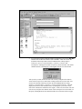
Building a 32-Bit Delphi Pascal Program ................................................................................96
Building a 16-Bit Delphi Pascal Program ................................................................................98
Delphi Pascal Example Source Code .......................................................................................98
Calling the Solver DLL from FORTRAN
103
FORTRAN Compilers ...........................................................................................................103
Basic Steps.............................................................................................................................103
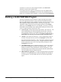
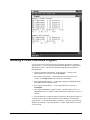
Building a 32-Bit FORTRAN Program .................................................................................104
Building a 16-Bit FORTRAN Program .................................................................................105
FORTRAN Example Source Code ........................................................................................106
ii • Introduction
Dynamic Link Library Solver User's Guide
Solver API Reference
109
Overview................................................................................................................................ 109
Argument Types ...................................................................................................... 110
NULL Values for Arrays ......................................................................................... 110
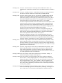
Problem Definition Routines ................................................................................................. 111
loadlp....................................................................................................................... 111
loadquad .................................................................................................................. 113
loadctype ................................................................................................................. 114
loadnlp ..................................................................................................................... 114
loadnltype ................................................................................................................ 116
testnltype.................................................................................................................. 117
unloadprob............................................................................................................... 118
Solution Routines................................................................................................................... 118
optimize ................................................................................................................... 119
mipoptimize............................................................................................................. 119
solution .................................................................................................................... 119
objsa ........................................................................................................................ 121
rhssa......................................................................................................................... 121
varstat ...................................................................................................................... 122
constat...................................................................................................................... 122
Diagnostic Routines ............................................................................................................... 123
findiis....................................................................................................................... 123
getiis ........................................................................................................................ 124
iiswrite ..................................................................................................................... 124
lpwrite...................................................................................................................... 125
lpread....................................................................................................................... 125
Use Control Routines............................................................................................................. 127
getuse....................................................................................................................... 128
reportuse .................................................................................................................. 128
getproblimits............................................................................................................ 129
Callback Routines for Nonlinear Problems............................................................................ 130
funceval ................................................................................................................... 130
jacobian ................................................................................................................... 131
Other Callback Routines ........................................................................................................ 132
setlpcallbackfunc ..................................................................................................... 132
getlpcallbackfunc..................................................................................................... 133
setmipcallbackfunc .................................................................................................. 133
getmipcallbackfunc.................................................................................................. 133
getcallbackinfo ........................................................................................................ 133
Solver Parameters .................................................................................................................. 134
Integer Parameters (General)................................................................................... 134
Integer Parameters (Solver Engines) ....................................................................... 135
Integer Parameters (Mixed-Integer Problems)......................................................... 138
Double Parameters................................................................................................... 139
setintparam .............................................................................................................. 141
getintparam .............................................................................................................. 141
infointparam ............................................................................................................ 141
setdblparam ............................................................................................................. 142
getdblparam ............................................................................................................. 143
infodblparam............................................................................................................ 143
setdefaults ................................................................................................................ 144
Dynamic Link Library Solver User's Guide
Contents • iii
Introduction
The Solver Dynamic Link Libraries
Welcome to Frontline Systems’ Small-Scale Solver Dynamic Link Library (DLL).
The Solver DLL provides the tools you need to solve linear, quadratic, nonlinear, and
nonsmooth optimization problems, and mixed-integer problems of varying size. It
can be called from a program you write in any programming language, macro
language, or scripting language for Microsoft Windows that is capable of calling a
DLL. Some of the possibilities that will be covered in this User Guide are Microsoft
Visual C++, Visual Basic, Delphi Pascal, and Fortran Powerstation. There are many
others, including Visual Basic Application Edition in each of the Microsoft Office
applications.
Frontline offers two Solver DLL product lines with compatible calling conventions:
the Small-Scale Solver DLL, which handles smaller, “dense matrix” problems, and
the Large-Scale Solver DLL, which handles larger, “sparse matrix” problems.
The Small-Scale Solver DLL handles linear and quadratic programming problems
with up to 2000 decision variables, depending on the version, and nonlinear and
nonsmooth optimization problems of up to 400 decision variables. (Any of the
variables may be general integer or binary integer.) It is offered in five different
configurations that include only the Solver “engines” (linear, quadratic and/or
nonlinear/nonsmooth) that you need for your application.
The Large-Scale Solver DLL handles linear and mixed-integer linear programming
problems of up to 16,384 decision variables. At present, the Large-Scale Solver DLL
does not include facilities for solving quadratic, nonlinear, or nonsmooth
optimization problems, but future versions may include these capabilities.
Both Solver DLLs are offered in 32-bit versions for Windows 95/98 and Windows
NT/2000 and in 16-bit versions for Microsoft Windows 3.1. (You can also run 16bit applications, which call the 16-bit Solver DLLs, under Windows 95/98 or NT.)
The Small-Scale Solver DLL
Frontline’s Small-Scale Solver DLL is a compact and efficient solver for linear
programming (LP), mixed integer programming (MIP), and optionally quadratic
programming (QP) problems of up to 2000 decision variables, depending on the
version, and smooth nonlinear programming (NLP) problems or nonsmooth
Dynamic Link Library Solver User's Guide
Introduction • 5
optimization problems of up to 400 decision variables and 200 constraints (in
addition to bounds on the variables).
The Small-Scale Solver DLL is an enhanced version of the linear, mixed integer and
nonlinear programming “engine” used in the Microsoft Excel Solver, which was
developed by Frontline Systems for Microsoft. This Solver has been proven in use
over nine years in tens of millions of copies of Microsoft Excel. Microsoft selected
Frontline Systems' technology over several alternatives because it offered the best
combination of robust solution methods, performance and ease of use.
The Small-Scale Solver DLL is also a “well-behaved” Microsoft Windows Dynamic
Link Library. It respects Windows conventions for loading and sharing program
code. Under Windows NT/2000 or Windows 95/98, the Solver DLL runs in 32-bit
protected mode and supports preemptive multitasking. When used under Windows
3.1, the Solver DLL shares the processor with other applications through Windows
non-preemptive multitasking. It also solves the problems of 16-bit Windows memory
management through use of a “two-level” storage allocator, which draws upon
Windows global memory resources in an efficient manner.
The algorithmic methods used in the Small-Scale Solver DLL include:
•
Simplex method with bounds on the variables for linear programming problems
•
Very fast “exact” quadratic method for solving QP problems such as portfolio
optimization models
•
Generalized Reduced Gradient method for solving smooth nonlinear programming problems
•
Evolutionary Solver (based on genetic algorithms) for solving nonsmooth
optimization problems
•
Memory-efficient Branch & Bound method for mixed-integer problems
•
Preprocessing and Probing strategies for fast solution of zero-one integer
programming problems
•
Very fast on “sparse” LP models with fewer nonzero matrix coefficients
•
Automatic scaling, degeneracy control and other features for robustness
•
Sensitivity analysis (shadow prices and reduced costs) for linear, quadratic and
nonlinear problems
•
Optional objective coefficient and constraint right hand side sensitivity “range”
information for linear problems
•
Automatic diagnosis of infeasible linear and nonlinear problems, computing an
Irreducibly Infeasible Subset (IIS) of constraints
The Large-Scale Solver DLL
Frontline’s Large-Scale Solver DLL is a state of the art implementation of linear
programming (LP) and mixed-integer programming (MIP) solution algorithms. The
16-bit version of the Large-Scale Solver DLL can handle problems of up to 8,192
decision variables and 8,192 constraints in addition to bounds on the variables. The
32-bit version (which can be called from a 32-bit application under Windows 95/98
or NT/2000) can handle problems of up to 16,384 variables and 16,384 constraints.
The Large-Scale Solver DLL efficiently stores and processes LP models in sparse
matrix form. It uses modern matrix factorization methods to control numerical
6 • Introduction
Dynamic Link Library Solver User's Guide
stability during the solution of large LP models, where the cumulative effect of the
small errors inherent in finite precision computer arithmetic would otherwise
compromise the solution process. These same methods often result in solution
speeds far beyond earlier generations of LP solvers. Thanks to these methods, the
Large-Scale Solver DLL can readily handle all of the problems in the well-known
NETLIB test suite – virtually all with the default tolerance settings.
The Large-Scale Solver DLL is also a “well-behaved” Microsoft Windows Dynamic
Link Library. Like the Small-Scale Solver DLL, it respects Windows conventions
for loading and sharing program code. Under Windows NT/2000 or Windows 95/98,
the Solver runs in 32-bit protected mode and supports preemptive multitasking.
When used under Windows 3.1, the Large-Scale Solver DLL shares the processor
with other applications through Windows non-preemptive multitasking, and draws
upon Windows global memory resources in an efficient manner.
The Large-Scale Solver DLL uses many of the best published solution methods and
has been proven in use on large LP models in industry and government around the
world. These algorithmic methods include:
•
Simplex method with two-sided bounds on both variables and constraints
•
Memory-efficient Branch & Bound method for mixed-integer problems
•
Matrix factorization using the LU decomposition, with the Bartels-Golub update
•
Refactorization using dynamic Markowitz methods for speed and stability
•
Steepest-edge techniques which often substantially reduce the number of pivots
•
Sophisticated “crash-like” methods for finding an effective initial basis
•
Basis restart for faster solution of MIP subproblems
•
Automatic row and column scaling, plus control of various algorithm tolerances
The Large-Scale Solver DLL is described in a separate Solver User’s Guide, which is
available on request from Frontline Systems. In the rest of this User’s Guide, the
term “Solver DLL” refers to the Small-Scale version.
Which Solver DLL Should You Use?
The Solver DLL is offered in five different configurations that include only the
Solver “engines” (linear, quadratic, nonlinear and nonsmooth) that you need for your
application. The possible configurations are:
•
Linear (Simplex) Solver only
•
Nonlinear (GRG) plus Nonsmooth (Evolutionary) Solvers only
•
Both Linear (Simplex) Solver and Nonlinear (GRG) plus Nonsmooth
(Evolutionary) Solvers
•
Linear (Simplex) Solver plus Quadratic and MIP enhancements
•
Both Linear (Simplex) Solver plus Quadratic and MIP enhancements, and
Nonlinear (GRG) plus Nonsmooth (Evolutionary) Solvers
Linear Solver
The linear (LP) Solver is the preferred Solver “engine” for linear programming
problems. It uses the Simplex method to solve the problem, which is guaranteed (in
Dynamic Link Library Solver User's Guide
Introduction • 7
the absence of severe difficulties with scaling or degeneracy) to find the optimal
solution if one exists, or to find that there is no feasible solution or that the objective
function is unbounded.
The LP Solver is designed to accept a matrix of coefficients (called matval later in
this Guide) which allows the Solver itself to compute values for the problem
functions (objective and constraints). If you supply the matrix of coefficients, you
don’t have to write a function (funceval()) to evaluate the problem functions. In most
cases, the coefficients are readily available from the data accepted as input or
computed by your application. In other situations, the coefficients might not be so
readily available and you might find it easier to write a funceval() routine. If your
Solver DLL includes both the nonlinear (NLP) and LP Solver “engines,” you can ask
the Solver DLL to compute the matrix of coefficients for you, by calling your
funceval() routine, and then solve the problem using the faster and more reliable LP
Solver “engine.”
Quadratic Solver
The quadratic (QP) Solver is an extension to the LP Solver which solves quadratic
programming problems, such as portfolio optimization problems, with a quadratic
objective function and all linear constraints. It uses the fast and reliable Simplex
method to solve a series of subproblems leading to the optimal solution for the
quadratic programming problem.
The QP Solver is designed to accept a matrix of coefficients (matval) for the linear
constraints, and another matrix of coefficients (qmatval) for the quadratic objective
function. (In a portfolio optimization problem, the objective function is normally the
portfolio variance, and the qmatval coefficients are the covariances between pairs of
securities in the portfolio.)
If you wish to minimize variance in a portfolio optimization problem, the QP Solver
is the preferred Solver “engine” since it will be faster and more accurate than the
NLP Solver. If, however, you wish to maximize portfolio return and treat portfolio
variance as a constraint, your problem will not be a QP (since its constraints are not
all linear) and you will need to use the NLP Solver.
Nonlinear Solver
The nonlinear (GRG) Solver can solve smooth nonlinear, quadratic, and linear
programming problems. It may also be the easiest-to-use Solver “engine” if it is
natural for you to describe the optimization problem by writing a function (called
funceval() later in this Guide) that evaluates the objective and constraints for given
values of the decision variables.
However, this generality comes at a price of both speed and reliability: On smooth
nonlinear problems, the NLP Solver (like all similar gradient-based methods) is
guaranteed only to find a locally optimal solution which may or may not be the true
(globally) optimal solution within the feasible region.
Moreover, since the NLP Solver treats QP and LP problems as if they were general
nonlinear problems, it is likely to take considerably more time to solve such
problems, and it may find solutions which are less accurate or less exact than
solutions found by the Solver “engine” most appropriate to the task.
Problems such as poor scaling or degeneracy also cause greater difficulty for the
NLP Solver than for the QP or LP Solver. If you have a linear (or quadratic)
problem, or a mix of nonlinear and linear (or quadratic) problems, we highly
8 • Introduction
Dynamic Link Library Solver User's Guide
recommend that you experiment with each of the Solver “engines” and compare both
solution time and accuracy of the results.
Nonsmooth (Evolutionary) Solver
The nonsmooth (Evolutionary) Solver, based on genetic or evolutionary algorithms,
is the most general-purpose Solver “engine” in that it makes no assumptions about
the mathematical form of the problem functions (objective and constraints): They
may be linear, quadratic, smooth nonlinear, nonsmooth, or even discontinuous and
nonconvex functions. Moreover, for smooth nonlinear problems where the GRG
Solver is guaranteed to find only a locally optimal solution, the Evolutionary Solver
can often find a better, globally optimal solution. Like the nonlinear Solver, it calls a
function funceval() that you write to evaluate the objective and constraints for given
values of the decision variables.
However, this generality comes at a considerable price of both speed and reliability.
Unlike the Simplex and GRG Solvers which are deterministic optimization methods,
the Evolutionary Solver is a nondeterministic method: Because it is based partly on
random choices of trial solutions, it will often find a different “best solution” each
time you run it, even if you haven’t changed your problem at all. And unlike the
Simplex and GRG Solvers, the Evolutionary Solver has no way of knowing for
certain that a given solution is optimal – even “locally optimal.” Similarly, the
Evolutionary Solver has no way of knowing for certain whether it should stop, or
continue searching for a better solution – it is forced to rely on tests for slow
improvement in the solution to determine when to stop.
Solving Mixed-Integer Problems
The Branch & Bound method for solving mixed integer programming problems is
included in all configurations of the Solver DLL. It can call any of the classical
Solver “engines” to solve its subproblems – so you can solve integer linear problems
with the LP Solver, integer quadratic problems with the QP Solver, and integer
nonlinear problems with the NLP Solver. (The Evolutionary Solver “engine” handles
integer variables on its own, so the Branch & Bound method is not used in
conjunction with it.) Also, because the NLP Solver (or any similar method) is not
guaranteed to find the globally optimal solution to any subproblem, the Branch &
Bound method is not guaranteed to find the true optimal solution to an integer
nonlinear problem – though it will often find a “good” but not provably optimal
integer solution. Solving integer linear problems with the LP Solver, or integer
quadratic problems with the QP Solver, is an intrinsically faster and more reliable
process.
If you have an integer linear problem with many binary or 0-1 integer variables, we
recommend that you try solving it with a Solver DLL configuration that includes the
QP Solver. Packaged with the QP Solver are a set of Preprocessing and Probing
strategies for linear constraints that often greatly speed up the solution of problems
with many 0-1 integer variables.
16-Bit Versus 32-Bit Versions
The choice of 16-bit versus 32-bit versions of the Solver DLL will probably be
dictated by the programming language or other tool you are using to write your
application program. For example, Visual Basic 3.0 is a 16-bit system which can call
only the 16-bit Solver DLL, whereas Visual Basic for Applications as shipped with
Microsoft Office 95, 97 and 2000 can call only the 32-bit versions of the DLL.
Dynamic Link Library Solver User's Guide
Introduction • 9
The 32-bit versions of the Solver DLL takes full advantage of the instruction set
features of the Intel 386, 486, Pentium and above processors, yielding a speed
advantage which may be as great as a factor of two on larger problems.
Support for 16-bit versions of the Solver DLL will be limited in the future. We
highly recommend that you use the 32-bit versions of the Solver DLL and develop
your application for 32-bit platforms such as Windows 95/98 and Windows NT.
What’s New in Version 3.5
Version 3.5 of the Solver DLL product line introduces a number of new features
including the Evolutionary Solver, reentrant versions of the Solver DLL for multithreaded applications, routines to support use-based licensing for Web server and
similar applications, and the ability to read in and solve a linear, quadratic, or mixedinteger problem written in algebraic notation from a external text file.
Evolutionary Solver
The new Evolutionary Solver “engine,” included with the nonlinear GRG Solver in
Version 3.5 of the Solver DLL, is designed to find good – though not provably
optimal – solutions for problems where the “classical” gradient methods in the GRG
Solver are not sufficient. The GRG Solver assumes that the problem functions
(objective and constraints) are smooth functions of the variables (i.e. the gradients of
these functions are everywhere continuous); its guaranteed ability to converge to a
local optimum depends on this assumption. In problems with nonsmooth or even
discontinuous functions, the GRG Solver often has difficulty reaching a solution. In
such problems, the Evolutionary Solver – which makes no assumptions about the
problem functions – can often find a good solution. Even in smooth nonlinear
problems, the GRG Solver is guaranteed only to find a locally optimal solution, but it
may miss a better solution far from the starting point you provide. The Evolutionary
Solver has a much better chance of finding the globally optimal solution in such
problems.
Multi-Threaded Applications
Version 3.5 of the Solver DLL is offered in both single-threaded and multi-threaded
versions. The single-threaded versions – like all earlier versions of the Solver DLL –
are serially reusable but not reentrant: They can solve multiple problems serially, but
not concurrently, nor can they solve problems recursively, for example where
computation of the objective or constraints for one optimization problem involves
solution of another optimization subproblem. The multi-threaded versions of the
Solver DLL V3.5 are fully reentrant: They can solve multiple problems concurrently
and/or recursively. They are especially suitable for Web server or Intranet-based
applications, which may be accessed by many users at unpredictable moments which
may overlap in time.
Use-Based Licensing
With the ability to solve multiple problems concurrently, the Solver DLL Version 3.5
is being deployed in Web server and similar applications where the number of users
is unknown in advance, or may become very large. In such cases, the normal userbased (or “seat-based”) licensing for multiple copies of the Solver DLL may not be
appropriate. To meet this requirement, Frontline Systems has developed alternative
10 • Introduction
Dynamic Link Library Solver User's Guide
use-based licensing terms, which permit any number of users or seats, but which
monitor the number of uses or calls to the optimizer. Developers can choose userbased or use-based licensing. On either basis, they can prepay for a quantity of
licenses to bring down the average cost on a steeply declining discount schedule, and
they can arrange that the total license cost will not exceed a certain fixed amount for
a period such as a year, or for the lifetime of the application.
To support use-based licensing, certain configurations of the Solver DLL V3.5
include the ability to count uses (i.e. calls to the loadlp() or loadnlp() functions, and
calls to the optimize() or mipoptimize() functions) and report this information both to
the user and to Frontline Systems. Use information can be written to a text file or
emailed to Frontline Systems, either automatically or under the control of the
application program (via the new getuse() and reportuse() functions.)
Problems in Algebraic Notation
Previous versions of the Solver DLL featured the ability to write out a text file
containing an algebraic description of a linear, quadratic or mixed-integer problem.
The primary use of this feature was in testing and debugging an application program,
to ensure that the problem being defined by calls to the Solver DLL routines was in
fact the problem intended. Version 3.5 of the Solver DLL features the new lpread()
function to complement the lpwrite() or lprewrite() functions. With lpread(), the
application can read in a problem previously written to disk by lpwrite(), or a
problem generated in the correct format by another program or via hand editing of
the text file. This provides a wide range of new options for saving problems across
multiple sessions, and solving problems interactively or in combination with other
programs.
How to Use This Guide
This User Guide includes a chapter on installing the Solver DLL files, and a chapter
providing an overview of the Solver DLL API calls and how they may be used to
define and solve linear (LP), quadratic (QP), nonlinear (NLP), nonsmooth (NSP),
and mixed-integer (MIP) programming problems. It also includes chapters giving
specific instructions for writing, compiling and linking, and testing application
programs in four languages: C/C++, Visual Basic, Delphi Pascal, and FORTRAN.
We highly recommend that you read the installation instructions and the overview of
the Solver DLL API calls first. Then you may turn directly to the chapter that covers
the language of your choice. Each chapter gives step-by-step instructions for
building and testing a simple example program – included with the Solver DLL –
written in that language. You can use these example programs as a starting point for
your own applications.
The chapter “Solver API Reference” provides comprehensive documentation of all of
the Solver DLL’s Application Program Interface (API) routines. It covers many
details besides those features illustrated in the various example applications. You’ll
want to consult this chapter as you develop your own application.
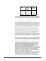
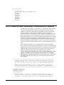
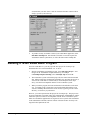
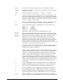
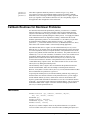
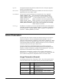
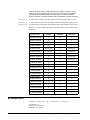
Included with the Solver DLL are source code header files (defining the Solver DLL
callable routines) and source code for example programs in four languages: C/C++,
Visual Basic, Delphi Pascal, and FORTRAN.
Dynamic Link Library Solver User's Guide
Introduction • 11
Language
Example File
Header File
C/C++
vcexamp1.c,
vcexamp2.c
frontmip.h
Visual Basic
vbexamp1.vbp,
vbexamp2.vbp
frontmip.bas,
safrontmip.bas
Delphi Pascal
psexamp.dpr
frontmip.pas
FORTRAN
flexamp.for
frontmip.for
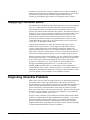
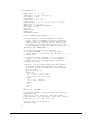
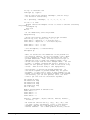
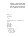
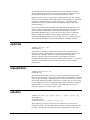
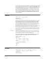
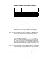
For all four languages, the example programs define and solve two optimization
problems – a simple LP (linear programming) problem, and a simple NLP (nonlinear
programming) problem. (Note: If your version of the Solver DLL includes only the
LP or only the NLP Solver engine, you will be able to solve only one of these two
problems; the other will display an error message dialog.) For C/C++ and Visual
Basic, more extensive examples are included as outlined below.
For C/C++ and FORTRAN, the example files are text files containing source code;
the instructions in the appropriate chapters explain how to create a project that will
compile, link and run the sample programs. For Visual Basic and Delphi Pascal –
which are designed to create forms-oriented applications – a complete project with
supporting files is included. These projects create simple forms that display the
results of solving the two optimization problems when a button is pressed.
The example programs for C/C++ and Visual Basic provide a total of eleven
examples of using the Solver DLL. The first set (source code file vcexamp1.c or VB
project vbexamp1.vbp) includes five examples: (1) A simple two-variable LP
problem, (2) A simple MIP (mixed-integer linear programming) problem, (3) An
example illustrating the Solver DLL features for diagnosing infeasibility, (4) A
simple quadratic programming problem, which uses the classic Markowitz method to
find an efficient portfolio of five securities, and (5) An example using the lpread()
function to read and solve a problem defined in algebraic notation in an external text
file.
The second set (source code file vcexamp2.c or VB project vbexamp2.vbp) includes
four examples of nonlinear problems, plus two examples of nonsmooth problems:
(1) A simple two-variable NLP problem, (2) The same NLP problem with an optional
user-written routine for computing partial derivatives, (3) An example illustrating the
diagnosis of infeasibility for nonlinear problems, (4) An example showing how you
can solve a series of linear and nonlinear problems, testing them for linearity, and
switching between the NLP and LP Solver engines, (5) An example where the
Evolutionary Solver finds the global minimum of a function with several local
minima, and (6) An example where the Evolutionary Solver finds the optimal
solution to a problem with a nonsmooth (discontinuous) objective.
If you are using the 16-bit version of the Solver DLL, and you are either solving a
large-scale problem or you wish to use the “callback functions” to gain control during
the solution process, be sure to read the chapter “Special Considerations for
Windows 3.x” – even if you are running your 16-bit application under Windows
95/98 or NT/2000 in Windows 3.x compatibility mode.
The chapter “Native Windows Applications” provides the C source code of a native
Windows application, written to the Win16/Win32 API. This source code can be
compiled into either a 16-bit or 32-bit application, and run under Windows 3.x,
Windows 95/98 or Windows NT/2000. It makes use of the Solver DLL’s callback
12 • Introduction
Dynamic Link Library Solver User's Guide
functions, and takes into account the special considerations for Windows 3.x. Also
included in this chapter is the C source code of a simple multi-threaded application
calling the reentrant version of the Solver DLL, written to the Win32 API.
Dynamic Link Library Solver User's Guide
Introduction • 13
Installation
Running the Installation Program
Most versions of the Solver DLL are provided in the form of single executable
installation program file, such as SolvLP.exe, that can be run to uncompress and
install all of the Solver DLL files, library and header files, and example source code
files discussed later in this User Guide. The name of the executable file reflects the
configuration of the Solver DLL you ordered from Frontline Systems:
SolvLP.exe – Linear (Simplex) Solver only
SolvNp.exe – Nonlinear (GRG) plus Nonsmooth (Evolutionary) Solvers only
SolvNpLp.exe – Both Linear (Simplex) Solver and Nonlinear (GRG) plus
Nonsmooth (Evolutionary) Solvers
SolvLpQp.exe – Linear (Simplex) Solver plus Quadratic and MIP enhancements
SolvNpLpQp.exe – Both Linear (Simplex) Solver plus Quadratic and MIP
enhancements, and Nonlinear (GRG) plus Nonsmooth (Evolutionary) Solvers
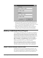
Simply run this executable program to install the Solver DLL files into the directory
structure outlined in the next section (for manual installation). The installation
program will prompt you for two pieces of information:
•
An installation password
•
A 16-character license key string, specific to your application(s)
Both pieces of information are included in the physical package you received from
Frontline Systems, or they may be provided to you by phone, fax or email. Carefully
enter the license key string exactly as given to you – use uppercase for any letters. If
you have any questions, please contact Frontline Systems as shown on the inside title
page of this User Guide.
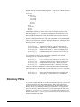
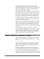
Copying Disk Files Manually
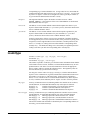
The Solver DLL files can be provided in uncompressed form on floppy disk, so they
may be copied to a convenient directory on your hard disk with standard Windows
commands. We recommend that you create a directory FRONTMIP in your hard
disk root directory (e.g. c:\frontmip if your hard disk drive letter is c:) and
copy the entire contents of the distribution floppy disk to this directory. You can
Dynamic Link Library Solver User's Guide
Installation • 15
drag and drop the files in the Windows Explorer, or you can use the DOS command
xcopy a:\*.* c:\frontmip /s. The resulting directory structure is:
Frontmip
Examples
Flexamp
Psexamp
Vbexamp
Vcexamp
Win16
Win32
Help
Include
Win16
Win32
The Examples subdirectory contains source code for example programs in four
different languages: C/C++, Visual Basic, Delphi Pascal, and FORTRAN. The
Win16 and Win32 subdirectories within the Examples directory hold compressed
archives (examples.zip) containing 16-bit and 32-bit executable of the example
programs, compiled from the source code, plus a compatible version of frontmip.dll.
The Include subdirectory contains an appropriate header file, declaring the Solver
DLL entry points, for each language:
frontmip.h
frontmip.bas
safrontmip.bas
frontmip.pas
frontmip.for
frontcbi.for
C/C++ header file – reference in your source code
Visual Basic header file – add to your VB project
VB header file w/SAFEARRAYs – add to your project
Delphi Pascal header file – add to your Delphi project
FORTRAN header file – reference in your source code
FORTRAN header file – use with callback functions
It also contains a license key file, which declares a character string constant
containing your own, customized license key:
frontkey.h
frontkey.bas
frontkey.pas
frontkey.for
C/C++ license key file – reference in your source code
Visual Basic license key file – add to your VB project
Delphi Pascal license key file – add to your project
FORTRAN license key file – reference in your source
The Win16 and Win32 subdirectories contain the Solver DLL and import library
files. These files have the same names in each subdirectory, but Win16 contains 16bit versions and Win32 contains 32-bit versions of the files:
frontmip.dll
frontmip.lib
Solver DLL (Dynamic Link Library) executable code
Import library – used by linker in C++/FORTRAN
Directory Paths
As you write, compile and link, and execute your application program, you will need
to reference the Solver DLL files mentioned above. Since only single files are
needed at each step, you may find it convenient to copy the Solver DLL files to the
directory where you are building or running your application. If your application
may be run from many different directories, you may wish to place the Solver DLL
file in the c:\windows or c:\windows\system directory in Windows 3.x or
Windows 95/98, or the c:\winnt\system32 directory (for the 32-bit version of
the DLL) in Windows NT/2000.
16 • Installation
Dynamic Link Library Solver User's Guide
•
When you compile the program that calls the Solver DLL routines you will
reference the appropriate header file: frontmip.h, frontmip.bas,
safrontmip.bas, frontmip.pas or frontmip.for.
•
If you are using “load-time dynamic linking,” when you link the program that
calls the Solver DLL routines you will use the import library frontmip.lib.
If you are using “run-time dynamic linking,” the import library is not used. Note
that Visual Basic and Delphi Pascal use run-time dynamic linking.
•
When you execute the program that calls the Solver DLL routines, you will
reference the dynamic link library file frontmip.dll. No other files are
needed at execution time.
Licensing the Solver DLL
Please bear in mind that in order to lawfully distribute copies of the Solver DLL
within your organization or to external customers, or to lawfully use the Solver
DLL in a server-based application that serves multiple users, you will need an
appropriate license from Frontline Systems. Licenses to use and/or distribute the
Solver DLL in conjunction with your application are available at substantial
discounts that increase with volume. As discussed in the Introduction, you have the
option of choosing either user-based (“seat-based”) or use-based licensing. Please
contact Frontline Systems for licensing and pricing information.
The copy of the Solver DLL that you license, either for development purposes or
for distribution, is customized for use by your application program(s). It
recognizes a specific 16-character license key string which you provide as the
probname argument to the loadlp() or loadnlp() function. Without this license key
string, the Solver DLL will not function – all Solver DLL routines will return without
doing anything. It is important that you keep your license key string confidential, and
use it only in your application programs. Frontline Systems will treat you as
responsible for the use of any copies of the Solver DLL that recognize your specific
license key string.
Registry Entries for Use-Based Licensing
If you have chosen use-based licensing, you’ll receive a version of the Solver DLL
that is designed to count the number of uses (i.e. calls to the loadlp() or loadnlp()
functions, or calls to the optimize() or mipoptimize() functions) over time, and report
this information both to you and to Frontline Systems. To maintain the counts across
different executions of your application, the Solver DLL uses several entries under a
single key in the system Registry. To use the Solver DLL on a given PC (e.g. your
development system, or a production server), you must first run a supplied program,
CreateUseKey.exe, to create the Registry key and associated entries.
To do this, simply select Start Run and type the path of this program (normally
C:\Frontmip\ CreateUseKey.exe). Assuming that it successfully creates the
Registry entries, this program displays a confirming MessageBox. If run more than
once on a given PC, it will display a MessageBox noting that the entries already exist
in the Registry, and it will not modify them. For complete information on the Solver
DLL’s Registry key and associated entries, see the description of the getuse()
function in the chapter “Solver API Reference.”
During development and testing of your application, you can run the Solver DLL in
“Evaluation/Test mode,” where it does not counts uses; in this mode, the DLL will
Dynamic Link Library Solver User's Guide
Installation • 17
not reference the Registry entries, so they need not exist on the development system.
Once the DLL is placed into production, it should be run in “Use Counting mode,”
where the Registry entries must be present. For information on how to set the mode
in which the Solver DLL runs, consult the section “Use-Based Licensing” in the
following chapter, “Designing Your Application.”
On Windows NT and Windows 2000 systems, the CreateUseKey.exe program must
be run under a user account with privileges to create Registry entries. Since the
Solver DLL only updates existing Registry entries, it does not need to run under an
account with these privileges.
18 • Installation
Dynamic Link Library Solver User's Guide
Designing Your Application
Calling the Solver DLL
This chapter provides an overview of the way your application program should call
the Solver DLL routines to define and solve an optimization problem. We’ll use the
syntax of the C programming language, but the order of calls, the names of routines,
the arguments, and most other programming considerations are the same in other
languages.
You build your application program with a header file, specific to the language you
are using, which declares the Solver DLL routines, their arguments and return values,
and various symbolic constants. At run time, your application program uses dynamic
linking to load the Solver DLL and call various routines within it. Details of the
process of compiling, linking and running your application with the Solver DLL are
provided in the chapters on the various languages.
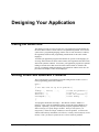
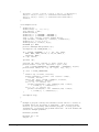
Solving Linear and Quadratic Problems
The overall structure of an application program calling the Solver DLL to solve a
linear programming problem is as follows:
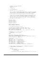
main()
{
/* Get data and set up an LP problem */
...
loadlp(..., matval, ...);
/* Load the problem
optimize(...);
/* Solve it
solution(...);
/* Get the solution
unloadprob(...);
/* Free memory
...
}
*/
*/
*/
*/
Your program should first call loadlp(). This function returns a “handle to a
problem.” Then you’ll call additional routines, passing the problem handle as an
argument. Optionally, you may call loadquad() to specify a quadratic objective,
and/or loadctype() to specify integer variables. Then you call optimize() (or
mipoptimize(), if there are integer variables) to solve the problem. To retrieve the
solution and sensitivity information, call solution(). Finally, call unloadprob() to free
memory. This cycle may be repeated to solve a series of Solver problems.
Dynamic Link Library Solver User's Guide
Designing Your Application • 19
When you call loadlp(), you pass information such as the number of decision
variables and constraints, arrays of (constant) bounds on the variables and the
constraints, an array of coefficients of the objective function, and a matrix of
coefficients (called matval above) of the constraint functions.
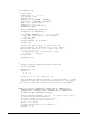
Solving Nonlinear Problems
In a linear or quadratic problem, you can describe the objective and constraints with
an array or matrix of constant coefficients; the Solver DLL can determine values for
the objective and constraints by computing the sums of products of the variables with
the supplied coefficients. In a nonlinear problem, however, the problem functions
cannot be described this way; the coefficients represent first partial derivatives of the
objective and constraints with respect to the variables, and these derivatives change
as the values of the variables change.
Hence, you must write a “callback” function (called funceval() below) that computes
values for the problem functions (objective and constraints) for any given values of
the variables. The Solver DLL will call this function repeatedly during the solution
process. You supply the address of this callback function as an argument to
loadnlp(), which defines the overall nonlinear optimization problem. You also
supply arrays for the objective and constraint coefficients (matval), as you do when
you call loadlp(), but these arrays need not be initialized to specific values – the
Solver DLL will fill them in when it calls your callback function(s). The overall
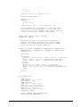
structure of a program calling the Solver DLL to solve a nonlinear programming
problem is:
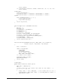
funceval(...)
{
/* Receive values for the variables, compute values */
/* for the constraints and the objective function
*/
}
main()
{
/* Get data and set up an LP problem */
...
loadnlp(..., funceval, ...);
/* Load the problem
optimize(...);
/* Solve it
solution(...);
/* Get the solution
unloadprob(...);
/* Free memory
...
}
*/
*/
*/
*/
Your program should first call loadnlp(). Like loadlp(), this function returns a
“handle to a problem.” Then you’ll call additional routines, passing the problem
handle as an argument. Optionally, you may call loadnltype() to give the Solver
more information about linear and nonlinear functions in your problem, testnltype()
to have the Solver determine the loadnltype() information through a numerical test, or
loadctype() to specify integer variables – defining an integer nonlinear problem.
Then call optimize() (or mipoptimize(), if there are integer variables) to solve the
problem. To retrieve the solution and sensitivity information, call solution().
Finally, call unloadprob() to free memory. As with loadlp(), this cycle may be
repeated to solve a series of Solver problems.
20 • Designing Your Application
Dynamic Link Library Solver User's Guide
Solving Nonsmooth Problems
You define and solve a problem with nonsmooth or discontinuous functions in much
the same way as you would for a problem defined by smooth nonlinear functions. In
a nonsmooth problem, however, the first partial derivatives of the objective and
constraints may not be continuous functions of the variables, and they may even be
undefined for some values of the variables. Because of this property, the gradientbased methods used by the nonlinear GRG Solver are not appropriate, and instead the
Evolutionary Solver “engine” must be used to solve the problem.
As for smooth nonlinear problems, you write a “callback” function funceval() that
computes values for the problem functions for any given values of the variables, and
you supply the address of this function as an argument to loadnlp(). But you cannot
use the optional jacobian() callback function (described below) to speed up the
solution of a nonsmooth problem.
Your program should first call loadnlp(), which returns a “handle to a problem.”
Then you must call loadnltype(), supplying this problem handle, to tell the Solver that
some or all of your problem functions are nonsmooth or discontinuous. This can be
as simple as:
loadnltype (lp, NULL, NULL); /* nonsmooth problem */
You may optionally call loadctype() to specify integer variables – defining an integer
nonsmooth problem. Then call optimize() (or mipoptimize(), if there are integer
variables) to solve the problem. To retrieve the solution and sensitivity information,
call solution(). Finally, call unloadprob() to free memory. This cycle may be
repeated to solve a series of Solver problems.
Genetic and Evolutionary Algorithms
A non-smooth optimization problem generally cannot be solved to optimality, using
any known general-purpose algorithm. But the Evolutionary Solver can often find a
“good” solution to such a problem in a reasonable amount of time, using methods
based on genetic or evolutionary algorithms. (In a “genetic algorithm,” the problem
is encoded in a series of bit strings that are manipulated by the algorithm; in an
“evolutionary algorithm,” the decision variables and problem functions are used
directly. Most commercial Solver products are based on evolutionary algorithms.)
An evolutionary algorithm for optimization is different from “classical” optimization
methods in several ways. First, it relies in part on random sampling. This makes it a
nondeterministic method, which may yield different solutions on different runs.
Second, where most classical optimization methods maintain a single best solution
found so far, an evolutionary algorithm maintains a population of candidate
solutions. Only one (or a few, with equivalent objectives) of these is “best,” but the
other members of the population are “sample points” in other regions of the search
space, where a better solution may later be found. The use of a population of
solutions helps the evolutionary algorithm avoid becoming “trapped” at a local
optimum, when an even better optimum may be found outside the vicinity of the
current solution.
Third – inspired by the role of mutation of an organism’s DNA in natural evolution –
an evolutionary algorithm periodically makes random changes or mutations in one or
more members of the current population, yielding a new candidate solution (which
may be better or worse than existing population members). There are many possible
ways to perform a “mutation,” and the Evolutionary Solver actually employs three
Dynamic Link Library Solver User's Guide
Designing Your Application • 21
different mutation strategies. The result of a mutation may be an infeasible solution,
and the Evolutionary Solver attempts to “repair” such a solution to make it feasible;
this is sometimes, but not always, successful.
Fourth – inspired by the role of sexual reproduction in the evolution of living things –
an evolutionary algorithm attempts to combine elements of existing solutions in order
to create a new solution, with some of the features of each “parent.” The elements
(e.g. decision variable values) of existing solutions are combined in a crossover
operation, inspired by the crossover of DNA strands that occurs in reproduction of
biological organisms. As with mutation, there are many possible ways to perform a
“crossover” operation – some much better than others – and the Evolutionary Solver
uses multiple variations of two different crossover strategies.
Fifth – inspired by the role of natural selection in evolution – an evolutionary
algorithm performs a selection process in which the “most fit” members of the
population survive, and the “least fit” members are eliminated. In a constrained
optimization problem, the notion of “fitness” depends partly on whether a solution is
feasible (i.e. whether it satisfies all of the constraints), and partly on its objective
function value. The selection process is the step that guides the evolutionary
algorithm towards ever-better solutions.
A drawback of an evolutionary algorithm is that a solution is “better” only in
comparison to other, presently known solutions; such an algorithm actually has no
concept of an “optimal solution,” or any way to test whether a solution is optimal.
(For this reason, evolutionary algorithms are best employed on problems where it is
difficult or impossible to test for optimality.) This also means that an evolutionary
algorithm has no definite rule for when to stop, aside from the length of time, or the
number of iterations or candidate solutions, that you wish to allow it to explore.
Aside from such limits, the Evolutionary Solver uses two heuristics to determine
whether it should stop – one based on the “convergence” of solutions currently in the
population, and the other based on the rate of progress recently made by the
algorithm. For more information, see the section “Solver Parameters” in the chapter
“Solver API Reference.”
Problems in Algebraic Notation
As outlined above, problems for the Solver DLL are generally defined by a series of
calls made by your application program. In particular, for linear and quadratic
problems, you must be careful to supply the correct values for objective and
constraint coefficients and constraint and variable bounds to define the problem you
want to solve. Problems you define exist only in main memory for the duration of
your calls to the Solver DLL – they do not “persist” across runs of your application.
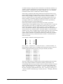
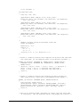
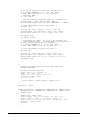
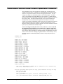
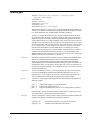
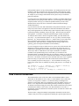
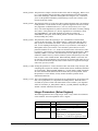
To make it easier to work with linear and quadratic problems, the Solver DLL can
read and write text files containing a problem description in a form very similar to
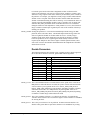
standard algebraic notation. An example of such a text file for a simple linear integer
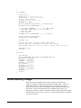
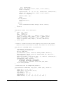
problem is shown below:
Maximize LP/MIP
obj: 2.0 x1 + 3.0 x2
Subject To
c1: 9.0 x1 + 6.0 x2 <= 54.0
c2: 6.0 x1 + 7.0 x2 <= 42.0
c3: 5.0 x1 + 10.0 x2 <= 50.0
Bounds
0.0 <= x1 <= +infinity
0.0 <= x2 <= +infinity
22 • Designing Your Application
Dynamic Link Library Solver User's Guide
Integers
x1
x2
End
If you define this problem via calls to loadlp() and loadctype(), you can produce a
text file with the contents shown above by calling lpwrite() or lprewrite(). (This
provides a convenient way to verify that the problem you defined programmatically
is the problem you intended, by examining the resulting text file.) If you have such a
text file containing your problem, you can define it by calling lpread(), without
setting up all of the array arguments normally required by loadlp() and loadctype().
You can use lpwrite() and lpread() to “persist” the definition of a problem on disk
between runs of your application program, without having to write code to store this
data in some file format of your own design. You can also use an external program
to generate a text file containing a problem definition in the format expected by
lpread(), then use the Solver DLL to read in the problem and solve it.
Using Other Solver DLL Routines
You can set various parameters and tolerances using the routines setintparam() and
setdblparam(), or get current, default, and minimum and maximum values for the
parameters with other routines.
To obtain control during the solution process (in order to display a message, check
for a user abort action, etc.), you can set the address of a callback routine through a
call to setlpcallbackfunc() (for any type of problem) or setmipcallbackfunc() (for
problems with integer variables). This feature – and the nonlinear Solver, which also
requires a callback routine – can be used only in languages, such as C/C++ and 32-bit
Visual Basic 5.0 and above, which permit you to define callback procedures and pass
procedure names as parameters.
Determining Linearity Automatically
As explained above, the primary difference between solving a nonlinear problem and
solving a linear problem is that you must provide a “callback” routine funceval() to
evaluate the nonlinear problem functions, at trial points (values for the variables)
determined by the Solver DLL. However, you do not have to initialize the arrays of
coefficients passed to loadnlp() with values.
It is possible to use loadnlp() and a funceval() routine for any Solver problem – even
if it is an entirely linear problem – but this will be significantly slower than calling
loadlp() for a linear problem, which employs the Simplex method.
If you are solving a specific problem or class of problems, you will probably know in
advance whether your problem is linear or nonlinear. If you know whether each
variable occurs linearly or nonlinearly in the objective and each constraint function,
you can supply this information to the Solver through loadnltype(). (Such
information can be used by advanced nonlinear solution algorithms to save time
and/or improve accuracy of the solution.)
If you are solving a general series of problems, however, you might have some
nonlinear and some linear problems, all represented by a funceval() routine. The
testnltype() routine lets you ask the Solver to determine, through a numerical test,
whether the problem is linear or nonlinear. In addition, testnltype() computes the
information you would otherwise have to supply through a call to loadnltype(), and if
Dynamic Link Library Solver User's Guide
Designing Your Application • 23
the problem is entirely linear, testnltype() computes the LP coefficients and places
them in the matval array that you supplied when you called loadnlp(). You can then
switch from the nonlinear Solver to the linear Simplex method by calling
unloadprob(), and calling loadlp() with the same arguments used for loadnlp().
Supplying a Jacobian Matrix
The nonlinear Solver algorithm uses the callback function funceval() in two different
ways: (i) to compute values for the problem functions at specific trial points as it
seeks an optimum, and (ii) to compute estimates of the partial derivatives of the
objective (the gradient) and the constraints (the Jacobian). The partial derivatives are
estimated by a “rise over run” calculation, in which the value of each variable in turn
is perturbed, and the change in the problem function values is observed. For a
problem with N variables, the Solver DLL will call funceval() N times on each
occasion when it needs new estimates of the partial derivatives (2*N times if the
“central differencing” option is used). This often accounts for 50% or more of the
calls to funceval() during the solution process.
To speed up the solution process, and to give the Solver DLL more accurate
estimates of the partial derivatives, you can supply a second callback function
jacobian() which returns values for all elements of the objective gradient and
constraint Jacobian matrix in one call. The callback function is optional – you can
supply NULL instead of a function address – but if it is present, the Solver DLL will
call it instead of making repeated calls to funceval() to evaluate partial derivatives.
Writing a jacobian() function can be difficult – it is easy to make errors in computing
the various partial derivatives. To aid in debugging, the Solver DLL has the ability
to call your jacobian() function and compute its own estimates of the partial
derivatives by calling funceval(). It will compare the results and display error
messages for mismatching partial derivatives. To use this feature, set the
PARAM_DERIV parameter value to 3 (see the chapter “Solver API Reference”).
The Evolutionary Solver “engine,” which is used if any of your problem functions are
nonsmooth or discontinuous (as indicated by loadnltype()), does not make use of the
jacobian() function, even if you supply it as an argument to loadnlp().
Diagnosing Infeasible Problems
When a call to optimize() finds no feasible solution to your optimization problem, the
Solver DLL returns a status value indicating this result when you call solution().
This means that there is no combination of values for the variables that will satisfy all
of the constraints (and bounds on the variables) at the same time. If your model
correctly describes the real-world problem, it may be that no solution is possible
unless you can find a way to relax some of the constraints. But more often, this result
means that you made a mistake in specifying some constraint(s), such as indicating
‘G’ (for >=) when you meant to use ‘L’ (for <=).
If you have many constraints, it can be difficult to determine which of them contains
a mistake, or conflicts with some other (combination of) constraints. To aid you, the
Solver DLL includes a facility to find a subset of your constraints such that your
problem, with just those constraints, is still infeasible, but if any one constraint is
dropped from the subset, the problem becomes feasible. Such a subset of constraints
is called an Irreducibly Infeasible Set (IIS) of constraints.
24 • Designing Your Application
Dynamic Link Library Solver User's Guide
(Note: If a call to mipoptimize() finds no feasible solution, your first step in
diagnosing the problem should be to try to solve the “relaxation” of the MIP
problem, ignoring the integer restrictions on the variables. You can do this by calling
setintparam( lp, PARAM_RELAX, 1) before you call mipoptimize() again. If the
relaxation of the original problem is still infeasible, you can use the API calls
described in this section to isolate the infeasibility.)
To find an Irreducibly Infeasible Set of constraints, call the routine findiis(). This
routine returns the number of rows (constraints) and the number of columns (variable
bounds) contained in the IIS; these numbers should always be less than or equal to
the total number of constraints and bounds in your problem. In many cases, there
will be only a few constraints in the IIS, and by inspecting your code which sets up
these constraints, you can often quickly identify the source of the infeasibility.
To obtain the IIS itself, call the routine getiis(). This routine returns the indices of
the constraints and the indices of the variable bounds that are included in the IIS. If
you have both lower and upper bounds on the same variable(s), getiis() tells you
which bound is contributing to the infeasibility.
If your problem is a linear or quadratic programming problem (i.e. if you are calling
loadlp()), there is an even more convenient way to obtain the IIS: Call the routine
iiswrite(). This routine calls findiis() for you (if it has not already been called) and
then writes out a text file, in the same “algebraic” format used by lpwrite(), but
containing only the constraints and bounds that are included in the IIS. When you
use iiswrite(), you don’t have to write any code to analyze or display the information
returned by getiis().
In general, when a model is infeasible, there can be more than one subset of
constraints (possibly many subsets) that qualify as an IIS. Some of these will contain
fewer constraints than others, making them easier to analyze. However, finding the
“minimal-size” IIS can be computationally very expensive; hence, the IIS finder is
designed to find an IIS that contains as few constraints (rows) as possible in a
reasonable amount of time. Since variable bounds are easier to analyze than full
constraints, the IIS finder favors fewer rows over fewer bounds.
Solution Properties of Quadratic Problems
A quadratic programming (QP) problem is one in which the objective is a quadratic
function, and the constraints are all linear functions of the variables. A general
quadratic function may be written as the sum of a quadratic term xT Q x and a linear
term c x:
F(x) = xT Q x + c x
The matrix Q is the Hessian (matrix of second partial derivatives) of the objective
function. Because the function is quadratic or second degree, all elements of this
matrix are constant. You supply the elements of the Q matrix when you call the
loadquad() function, and the elements of the c vector when you call the loadlp()
function (via the obj argument).
Depending on the properties of the Q matrix, a quadratic function may have one,
many, or no optimal (minimum or maximum) values. If the Q matrix is positive
definite (for a minimization problem; negative definite for a maximization problem),
the function will have a “bowl” shape and a single optimal solution (a strong
minimum). If the Q matrix is positive semi-definite, the function will have a “trough”
and (infinitely) many optimal solutions, all with the same objective function value (a
weak minimum). If the Q matrix is indefinite, the function will have a “saddle point”
Dynamic Link Library Solver User's Guide
Designing Your Application • 25
(which has many, but not all, of the properties of an optimal solution), however the
true optimal solution(s) – one or many of them – will lie somewhere on the
boundaries of the constraints.
Quadratic programming algorithms are specialized (for speed and accuracy) to solve
problems where the Q matrix is positive definite (when minimizing) or negative
definite (maximizing). The QP algorithm used in the Solver DLL is somewhat more
general: It can handle problems where the Q matrix is positive semi-definite (or
negative semi-definite), in which case it will converge to a point in the “trough” with
the correct minimum (maximum) objective function value. If applied to a problem
where the Q matrix is indefinite, however, the Solver DLL may converge either to a
saddle point, or to (one of) the optimal solution(s) on the constraint boundary –
depending on the initial values of the variables. In this case a call to the solution()
function will return a status code of PSTAT_FRAC_CHANGE to indicate that the
solution is not necessarily optimal.
The loadquad() function tests the Q matrix you supply to determine whether it is
positive (negative) definite, semi-definite or indefinite. If it is indefinite, loadquad()
will return a nonzero value, and if you have set the PARAM_ARGCK parameter to
warn about errors in the arguments, it will display an error message dialog.
Most problems based on real-world data yield a Q matrix which is positive definite.
For example, if you are solving a portfolio optimization problem where the Q matrix
represents variances and covariances of pairs of securities calculated from a historical
price series, it can be shown that the matrix will be positive definite if the number of
observations in the price series is greater than the number of variables.
If, however, you are solving problems based on arbitrary user-provided data, you
should take care to test the return value of the loadquad() function and the status
value returned by the solution() function. If the Q matrix is indefinite, you may wish
to use the nonlinear Solver “engine” instead of the quadratic Solver “engine” – but
you must bear in mind that either solution algorithm will find only a local optimum
which is not necessarily the global optimum.
The loadquad() function also accepts a var argument which provides initial values
for the variables. If the problem is positive (negative) semi-definite or indefinite,
these initial values will influence the path taken by the solution algorithm and the
final solution to which it converges. If you must solve problems of this type, you can
use the var argument to exercise some control over the solutions returned by the
Solver DLL.
Passing Dense and Sparse Array Arguments
In most large optimization problems, the constraint coefficient matrix (the Jacobian)
(and – in some quadratic problems – the Q matrix) are sparse – meaning that most of
the matrix elements are zero. For example, in many larger problems there are groups
of constraints that are functions of a small subset of the variables, but that do not
depend on any of the other variables – leading to many zero coefficients in the
constraint matrix.
When these matrices are sparse, it is more efficient to store – and to process – only
the nonzero matrix elements. A common way of doing this is to have auxiliary arrays
that supply the row and column indices of the nonzero elements. This means that no
storage at all is needed for the zero elements, which can include 90% to 95% of all
elements in large, sparse problems.
26 • Designing Your Application
Dynamic Link Library Solver User's Guide
For further memory savings, the nonzero elements can be ordered by column (i.e. by
variable), so that the column index need be stored only once for a set of consecutive
nonzero elements. (Alternatively, they could be ordered by row, i.e. by constraint;
but the Solver DLL uses the “column-wise” method of storage.)
In the loadlp(), loadquad() and loadnlp() functions, the Solver DLL allows you to
pass the constraint matrix (and the Q matrix, if used), in either dense or sparse form.
In dense form, you supply a “full-size” array of numcols * numrows elements
(numcols2 elements in the case of the Q matrix), which may include both zero and
nonzero elements; you need not supply any auxiliary information. In sparse form,
you supply a smaller array containing only the nonzero elements, plus auxiliary
arrays which provide the row and column indices.
In the loadlp() function (loadquad() and loadnlp() are similar), you pass the
constraint matrix via the arguments matbeg, matcnt, matind and matval. To pass the
matrix elements in dense form, you supply NULL values for matbeg, matcnt and
matind, and you supply a “full-size” array of numcols * numrows elements for
matval. Note that matval must be a single-dimensioned array where the elements are
stored so that the row (constraint) index is varied most rapidly. To pass the matrix
elements in sparse form, you supply arrays for all four of matbeg, matcnt, matind and
matval. The matbeg array contains column (variable) indices; the matcnt array
contains counts of elements in a column; the matind array contains row (constraint)
indices; and the matval array contains the nonzero elements. All column and row
indices are 0-based.
As an example, consider the following sparse matrix:
1.2
0.0
7.8
0.0
0.0
5.6
0.0
9.0
3.4
0.0
0.0
0.0
Here, numcols = 3 and numrows = 4; there are nzspace = 5 nonzero elements. To
pass this matrix in sparse form, you’d supply matbeg and matcnt arrays (of numcols
elements) and matind and matval arrays (of nzspace elements), as follows:
matbeg[0] = 0
matbeg[1] = 2
matbeg[2] = 4
matcnt[0] = 2
matcnt[1] = 2
matcnt[2] = 1
matind[0] = 0
matind[1] = 2
matind[2] = 1
matind[3] = 3
matind[4] = 0
matval[0] = 1.2
matval[1] = 7.8
matval[2] = 5.6
matval[3] = 9.0
matval[4] = 3.4
The array element matbeg[j] contains offsets from the beginning of the matind and
matval arrays where the nonzero coefficients of variable j will be found. The
corresponding element matcnt[j] contains a count of consecutive elements of matind
and matval which pertain to the same variable (i.e. are in the same column of the
matrix). Note that matbeg[j+1] = matbeg[j] + matcnt[j] – the Solver DLL checks
the arrays you supply to ensure that this is true. For k = matbeg[j] to matbeg[j+1] 1, there is a nonzero coefficient M[i,j] at column j and row i = matind[k], with value
matval[k].
Dynamic Link Library Solver User's Guide
Designing Your Application • 27
Arrays and Callback Functions in Visual Basic
The Solver DLL uses the calling conventions standardized for the Windows API
routines, which use argument data types drawn from C/C++. In particular, array
arguments are passed as pointers to the base of the block of memory containing the
array values.
In Visual Basic, however, arrays declared in the language are created using the COM
Automation conventions for SAFEARRAYs. A SAFEARRAY consists of a block of
memory called an array descriptor, which contains information about array element
sizes, dimensions and bounds, and a pointer to the memory holding the array values.
Visual Basic programs that call Windows API routines usually handle array
arguments by declaring the argument as ByRef and passing the first element of the
array (rather than the “whole” array) as the argument. For example, obj(0) passed
by reference is a pointer to the first array element, i.e. the base address of the block
of memory holding the array values; the SAFEARRAY descriptor is stored elsewhere
in memory by Visual Basic and is not “seen” by the Solver DLL. The Solver DLL is
able to access additional array elements beyond the first element by indexing into the
block of memory holding the array data.
This approach does not work in reverse, however: When Visual Basic is used to
write a callback function such as funceval() or jacobian(), where the Solver DLL
makes the call and passes blocks of memory for C-style arrays as arguments, the
Visual Basic code can reference only the first array element. Subscripting in Visual
Basic is permitted only if the argument is actually declared as an array (e.g. obj()),
and in this case Visual Basic expects to receive a SAFEARRAY as the argument.
(This argument must be a pointer to a pointer to the SAFEARRAY descriptor.)
To permit callback functions to be written in Visual Basic, the Solver DLL provides
an option to treat all arrays as SAFEARRAYs rather than C-style arrays. To use this
option, call setintparam() as shown below, before calling loadlp(), loadnlp() or any
of the other problem setup routines:
ret = setintparam( NULL, PARAM_ARRAY, 1 )
When this parameter is set to 1, all arrays passed to the Solver DLL must be
SAFEARRAYs. In Visual Basic, this means that the array arguments must be
declared as (for example):
ByRef obj() As Double
rather than
ByRef obj As Double
and the array name (e.g. obj), instead of the first array element (e.g. obj(0) )
must be passed as the actual argument. In your callback routines, you can then use
subscripting to refer to elements of the arrays passed to you as arguments.
The Visual Basic header file frontmip.bas contains declarations of the Solver
DLL routines that define the arguments as C-style arrays. The header file
safrontmip.bas contains declarations of the routines that define the arguments
as SAFEARRAYs. If you are using Visual Basic for a new Solver DLL application,
you will probably want to use safrontmip.bas as your header file (and be sure
to call setintparam( NULL, PARAM_ARRAY, 1 ) before calling other Solver DLL
routines).
28 • Designing Your Application
Dynamic Link Library Solver User's Guide
Using the Solver DLL in Multi-Threaded Applications
The Solver DLL is offered in both single-threaded and multi-threaded versions. The
single-threaded versions are serially reusable but not reentrant: They can solve
multiple problems serially – a call to loadlp() or loadnlp() must be followed by a call
to unloadprob() before the next call to loadlp() or loadnlp() is encountered.
The multi-threaded versions of the Solver DLL are fully reentrant. They can solve
multiple problems concurrently: You may call loadlp() or loadnlp() several times,
keeping track of the “problem handles” returned by each call, and freely mix calls to
any of the other Solver DLL routines, passing the appropriate problem handle to each
call. (You must still call unloadprob() for each problem handle when you are
finished with it, to release memory.)
The multi-threaded versions may be used to solve decomposition problems (which
involve both a “master problem” and a “slave problem”), or any recursive problem
where the computation of the objective or constraints for a main problem requires the
solution of another optimization subproblem. The multi-threaded versions may also
be used in Web server or Intranet applications, where the application calling the
Solver DLL consists of several threads of execution executing concurrently, each
thread dealing with a specific user session.
Use of the multi-threaded versions is identical to use of the single-threaded versions,
except that calls to loadlp() or loadnlp() that would return an error in the singlethreaded versions (because a previous problem had not yet been unloaded) will return
a new, valid “problem handle” without an error in the multi-threaded versions. Your
application simply needs to keep track of each problem handle, for example by
saving it in local variable storage that is unique to each thread of your program.
Use-Based Licensing
The Solver DLL can be licensed for distribution to multiple users with your
application, or for use on a server where the application serves multiple users.
Licensing for a server-based application is usually based on the number of users (or
“seats”). However, if this number is difficult to determine or if it may be very large –
as in a Web server application – licensing may be based on the number of uses of the
DLL. To support this latter form of licensing, the Solver DLL can track and report
the number of calls your application makes to the loadlp() / loadnlp() routines and/or
the optimize() / mipoptimize() routines.
Use tracking and reporting is under the control of your application. You determine
the type of tracking and reporting with a call such as:
ret = setintparam( NULL, PARAM_USERP, 1)
If the PARAM_USERP parameter is set to 0 (the default setting), the Solver DLL
does not track uses – it operates in “Evaluation / Test mode,” where it displays a
MessageBox on the system console once every ten minutes. If PARAM_USERP is
1, the Solver DLL does track uses; the first time it runs in a new calendar month, it
automatically sends a report of cumulative uses to date via email to Frontline
Systems. If PARAM_USERP is 2, the Solver DLL tracks uses, but it does not
generate any reports automatically – use reports are created only when your
application calls the reportuse() function, which can either write a text file or send an
email message, containing a report of cumulative uses.
Dynamic Link Library Solver User's Guide
Designing Your Application • 29
Calling the Solver DLL from
C/C++
C/C++ Compilers
To use the Solver DLL from C or C++, you must have an appropriate compiler and
linker capable of building Windows applications, such as Microsoft Visual C++,
Borland C++, Symantec C++ or WATCOM C++. This Guide will give explicit
instructions for use with Microsoft Visual C++ 5.x and 6.x (32-bit) and Visual C++
1.5x (16-bit), but use with other compilers should be similar.
Most C++ compilers for Windows allow you to easily port DOS or UNIX C and C++
applications (which use printf or cout for “glass teletype” output) to Windows. To
simplify the input/output and focus on the Solver DLL routines and arguments, the
example applications in this chapter use printf calls for output and will be built as
“Win32 console applications” in Microsoft Visual C++ (or as “QuickWin”
applications in 16-bit Visual C++).
To build a native Windows application in C or C++, you’ll have to learn something
about the Windows API and/or a C++ class library such as the Microsoft Foundation
Classes. A single-threaded and a multi-threaded example application using the
Windows API and the Solver DLL’s callback functions are presented in the later
chapter “Native Windows Applications.”
Basic Steps
To create an application that calls the Solver DLL, you must perform the three
following steps:
1.
Include the header file frontmip.h in your C or C++ source program. (You
should also include the license file frontkey.h to obtain the license key string.)
2.
Include the import library file frontmip.lib in your project or your linker
response file. (Alternatively, you can write code to use “run-time dynamic
linking” by calling Windows API routines such as LoadLibrary().)
3.
Call at least the routines loadlp() or loadnlp(), optimize(), solution() and
unloadprob() in that order.
Dynamic Link Library Solver User's Guide
Calling the Solver DLL from C/C++ • 31
You can use any of the example programs as a guide for getting the arguments right.
Vcexamp1.c contains five examples of solving linear, integer and quadratic
programming problems, including an example using the infeasibility (IIS) finder, an
example of portfolio optimization using the QP Solver, and an example that reads a
problem from a text file using the lpread() function. Vcexamp2.c contains four
examples of solving nonlinear programming problems, including an example using
the IIS finder and an example of testing a problem for linearity and switching
between the NLP and LP Solvers. It also contains two examples that use the
Evolutionary Solver to find the global optimum in a problem with multiple local
optima, and to find the optimum in a problem with nonsmooth functions.
Building a 32-Bit C/C++ Program
This section will outline the steps required to compile, link and run the example
Solver DLL application VCEXAMP1.EXE, using 32-bit Microsoft Visual C++ 5.x
or 6.x under Windows 95/98 or Windows NT/2000. The steps required to compile,
link and run VCEXAMP2.EXE are the same, and the steps involved in using other
C/C++ compilers will be similar.
First, follow the steps in the “Installation” chapter, which will copy the example
programs into the examples subdirectory of the frontmip directory on your hard
disk. If you wish, you can run the pre-built version of VCEXAMP1.EXE by doubleclicking on the filename, before you try to compile and link from the source code.
1.
Create a Project. Start Microsoft Visual Studio. Select File New... and in the
Projects tab of the displayed dialog, select Win32 Console Application. Type
vcexamp1 in the Project name edit box, and c:\frontmip\examples\vcexamp1
(or a path of your choosing) in the Location edit box. Then click OK. In Visual
C++ 6.x, click Finish and then OK in the New Project Wizard dialog boxes, to
create an empty project.
2.
Add Files. Select Project | Add to Project | Files... In the dialog, navigate if
necessary to the proper directory, select the file vcexamp1.c, and click OK.
Now select Select Project | Add to Project | Files... again. In the dialog, open the
Files of type dropdown list and select Library Files (*.lib). Navigate to the
Win32 subdirectory that contains the 32-bit version of the import library
frontmip.lib. Select frontmip.lib and click OK.
If you now select the FileView pane in the Project Workspace window and open
Vcexamp1 Files, the vcexamp1.c and frontmip.lib files should be listed. You
can double-click on vcexamp1.c to see the C source code.
3.
Build and Run the Application. To compile and link vcexamp1.c and produce
vcexamp1.exe, select Build Rebuild All. Then use Build Execute vcexamp1.exe
to run the program. An output window like the one on the next page should
appear. (Press the ENTER key to continue running the program and produce
more output.)
32 • Calling the Solver DLL from C/C++
Dynamic Link Library Solver User's Guide
Building a 16-Bit C/C++ Program
A 16-bit version of the example Solver DLL application VCEXAMP1.EXE, which
runs under Windows 3.x, may be built using Microsoft Visual C++ 1.5x. The steps
involved in using other 16-bit C/C++ compilers will be very similar
1.
Create a Project. Start Visual C++ 1.5x. Select Project New... In the New
Project dialog, click the Browse... button and navigate to the vcexamp1
subdirectory (this is c:\frontmip\examples\vcexamp1 in the default directory
structure). In the File name edit box, type vcexamp1.mak, then click OK.
Again in the New Project dialog, select QuickWin Application (.EXE) in the
Project Type dropdown list, ensure that “Use Microsoft Foundation Classes” is
not checked, and click OK.
2.
Add Files. The Project Edit dialog is immediately displayed. Navigate if
necessary to the proper directory, select the file vcexamp1.c, and click on Add.
In Visual C++ 1.5x, the Project Edit dialog remains open at this point.
Open the List Files of Type dropdown list and select Library (*.lib). Navigate to
the directory containing the 16-bit version of the import library frontmip.lib (in
the default directory structure, move two levels up and then down to Win16).
Select frontmip.lib and click on Add. Then click on Close.
If you want to examine the C source code, select File Open, navigate to the
appropriate directory if necessary, select vcexamp1.c and click OK.
3.
Build and Run the Application. To compile and link vcexamp1.c and produce
vcexamp1.exe, select Project Rebuild All VCEXAMP1.EXE. Then select
Project Execute VCEXAMP1.EXE to run the program. This QuickWin
application displays a window like the one shown on the next page. (Press the
ENTER key to continue running the program and produce more output.)
Dynamic Link Library Solver User's Guide
Calling the Solver DLL from C/C++ • 33
The first few lines of output have scrolled beyond the top of this window. You
should also note that the C source code in vcexamp1.c uses a callback function to
display the LP iterations only in the Win32 version of this example. In Windows 3.x,
you must set up callback function addresses with the MakeProcInstance API call.
This call requires an instance handle argument that is not readily available in a
QuickWin program. For an example of the use of callback functions in both Win32
and Win16 programs, see the chapter “Native Windows Applications.”
C/C++ Source Code: Linear / Quadratic Problems
The source code file vcexamp1.c is listed below. Note that it includes five example
problems for the Solver DLL, which are set up and solved in turn. The first example
is a simple two-variable LP problem. The second example – for which source code
in Visual Basic, Delphi Pascal and FORTRAN is also included – is a MIP problem,
identical to the previous LP problem except that the decision variables are required to
have integer values. The third example attempts to solve an LP problem that is
infeasible, then it uses the IIS finder to diagnose the infeasibility. The fourth
example is a quadratic programming problem, using the classic Markowitz method to
find an efficient portfolio of five securities. The fifth example uses the lpread()
function to read in a problem in “algebraic notation” from a text file that was created
by the lpwrite() function in the second example.
You are encouraged to study this source code (or the Visual Basic source code)
and the /* comments */ in each problem, even if you plan to use a language
other than C/C++ for most of your work. The C/C++ and Visual Basic example
code is more extensive than the examples for the other languages, and illustrates most
of the features of the Solver DLL including the Quadratic Solver, the Evolutionary
Solver, automatic diagnosis of infeasible problems, and use of the lpread() and
lpwrite() functions.
34 • Calling the Solver DLL from C/C++
Dynamic Link Library Solver User's Guide
/* **********************************************************************
Frontline Systems Small-Scale Solver Dynamic Link Library Version 3.5
Frontline Systems Inc., P.O. Box 4288, Incline Village, NV 89450 USA
Tel (775) 831-0300 ** Fax (775) 831-0314 ** Email [email protected]
Example LP, MIP and QP problems in C/C++: Build as Win32 console app
or Win16 QuickWin project containing files VCEXAMP1.C and FRONTMIP.LIB
********************************************************************** */
#include "frontmip.h"
#include "frontkey.h"
#include <stdio.h>
/*
Example 1: Solves the LP model:
Maximize
2 x1 + 3 x2
Subj to
9 x1 + 6 x2 <= 54
6 x1 + 7 x2 <= 42
5 x1 + 10 x2 <= 50
x1, x2 non-negative
LP solution: x1 = 2.8, x2 = 3.6
Objective = 16.4
This example shows the simple form of passing arguments to loadlp():
A dense (full-size N by M) matrix is passed as the matval argument
and NULL pointers are passed as the matbeg, matcnt & matind arguments.
This example also shows how to obtain LP sensitivity analysis info
by calling the objsa() and rhssa() functions. These calls are valid
only for LP problems. For QP problems, only dual values (the piout
and dj arguments of solution()) are available; for MIP problems, no
sensitivity analysis info is available (none would be meaningful).
This example uses a callback function to display the LP iterations.
*/
/* The following function is called on each LP iteration in example1 */
long _CC lpcallback (HPROBLEM lpinfo, long wherefrom)
{
long iters; double obj;
getcallbackinfo (lpinfo, wherefrom, CBINFO_ITCOUNT, (void*)&iters);
getcallbackinfo (lpinfo, wherefrom, CBINFO_PRIMAL_OBJ, (void*)&obj);
printf("Iteration %ld: Obj = %g\n", iters, obj);
return PSTAT_CONTINUE;
}
void example1(void)
{
double obj[] = { 2.0, 3.0 };
double rhs[] = { 54.0, 42.0, 50.0 };
char sense[] = "LLL"; /* L's for <=, E's for =, G's for >= */
double matval[] = { 9.0, 6.0, 5.0, 6.0, 7.0, 10.0 };
double lb[] = { 0.0, 0.0 };
double ub[] = { INFBOUND, INFBOUND };
long stat, i;
double objval;
double x[2], piout[3], slack[3], dj[2];
double varlow[2], varupp[2], conlow[3], conupp[3];
HPROBLEM lp = NULL;
printf("\nExample LP problem\n");
/* set up the LP problem */
Dynamic Link Library Solver User's Guide
Calling the Solver DLL from C/C++ • 35
lp = loadlp (PROBNAME, 2, 3, -1, obj, rhs, sense,
NULL, NULL, NULL, matval, lb, ub, NULL, 2, 3, 6);
if (!lp) return;
#ifdef WIN32
setlpcallbackfunc (lp, lpcallback); /* set up the callback */
#endif
/* solve the problem */
optimize (lp);
/* obtain the solution: display objective and variables */
solution (lp, &stat, &objval, x, piout, slack, dj);
printf("LPstatus = %ld Objective = %g\n", stat, objval);
/* display constraint slacks and dual values */
printf("x1 = %g x2 = %g\n\n", x[0], x[1]);
for (i = 0; i <= 2; i++)
printf("slack[%ld] = %7g piout[%ld] = %7g\n",
i, slack[i], i, piout[i]);
printf("\n");
/* obtain and display sensitivity analysis information */
objsa (lp, 0, 1, varlow, varupp);
for (i = 0; i <= 1; i++)
printf("Obj coefficient %3.0f Lower %7g Upper %7g\n",
obj[i], varlow[i], varupp[i]);
rhssa (lp, 0, 2, conlow, conupp);
for (i = 0; i <= 2; i++)
printf("Constraint RHS %3.0f Lower %7g Upper %7g\n",
rhs[i], conlow[i], conupp[i]);
printf("\n");
#ifdef WIN32
setlpcallbackfunc (lp, NULL); /* remove the callback function */
#endif
/* important - call unloadprob() to release memory */
unloadprob (&lp);
}
/*
Example 2: Solves the MIP model:
Maximize
2 x1 + 3 x2
Subj to
9 x1 + 6 x2 <= 54
6 x1 + 7 x2 <= 42
5 x1 + 10 x2 <= 50
x1, x2 non-negative, integer
MIP solution: x1 = 2, x2 = 4
Objective = 16.0
This example illustrates the full set of arguments, used to pass a
potentially sparse matrix to loadlp. For each variable (column) i,
matbeg[i] and matcnt[i] are the beginning index and count of nonzero coefficients in the matind and matval arrays. For each such
coefficient, matind[k] is the constraint (row) index and matval[i]
is the coefficient value. See the documentation for more details.
In this example, we also use two debugging features of the Solver
DLL: (1) We call setintparam() to enable the display of error
MessageBoxes by the DLL routines if they detect an invalid value
in one of the arguments we pass (since there are no errors, none
will appear). (2) We call lpwrite() to write out a file which
summarizes the LP/MIP problem in algebraic form. This can help
us verify that the arguments we pass have defined the right problem.
*/
36 • Calling the Solver DLL from C/C++
Dynamic Link Library Solver User's Guide
void example2(void)
{
double obj[] = { 2.0, 3.0 };
double rhs[] = { 54.0, 42.0, 50.0 };
char sense[] = "LLL";
long matbeg[] = { 0, 3 };
long matcnt[] = { 3, 3 };
long matind[] =
{
0,
1,
2,
0,
1,
2 };
double matval[] = { 9.0, 6.0, 5.0, 6.0, 7.0, 10.0 };
double lb[] = { 0.0, 0.0 };
double ub[] = { INFBOUND, INFBOUND };
char ctype[] = "II";
long stat;
double objval;
double x[2];
HPROBLEM lp = NULL;
printf("\nExample MIP problem\n");
/* enable display of error MessageBoxes on argument
errors (since the arguments are correct, none will
appear). Note - on argument errors, loadlp returns
a NULL pointer and all other routines return a nonzero value; you can and should check for this! But
the MessageBoxes can help you identify errors early. */
setintparam (lp, PARAM_ARGCK, 1);
/* set up the LP portion of the problem */
lp = loadlp (PROBNAME, 2, 3, -1, obj, rhs, sense,
matbeg, matcnt, matind, matval, lb, ub, NULL, 2, 3, 6);
if (!lp) return;
/* now define integer variables: for each variable i,
ctype[i] is 'C' for continuous, 'I' for general
integer and 'B' for a binary integer variable */
loadctype (lp, ctype);
/* lpwrite() can be called anytime after the problem
is defined, and before unloadprob() is called. It
will write out the following text in file vcexamp1:
Maximize LP/MIP
obj: 2.0 x1 + 3.0 x2
Subject To
c1: 9.0 x1 + 6.0 x2 <= 54.0
c2: 6.0 x1 + 7.0 x2 <= 42.0
c3: 5.0 x1 + 10.0 x2 <= 50.0
Bounds
0.0 <= x1 <= +infinity
0.0 <= x2 <= +infinity
Integers
x1
x2
End
*/
lpwrite( lp, "vcexamp1");
/* solve the problem; obtain and display the solution */
mipoptimize (lp);
solution (lp, &stat, &objval, x, NULL, NULL, NULL);
printf("LPstatus = %ld Objective = %g\n", stat, objval);
printf("x1 = %g x2 = %g\n", x[0], x[1]);
/* don't forget to free memory */
unloadprob (&lp);
}
/*
Dynamic Link Library Solver User's Guide
Calling the Solver DLL from C/C++ • 37
Example 3: Attempt to solve the LP model:
Maximize
2 x1 + 3 x2
Subj to
9 x1 + 6 x2 <= 54
6 x1 + 7 x2 <= 42
5 x1 + 10 x2 <= -50
x1, x2 non-negative
Infeasible (due to non-negative variables and negative RHS)
When solution() returns stat = PSTAT_INFEASIBLE, ask Solver DLL
to find an Irreducibly Infeasible Subset (IIS) of the constraints:
Row 2 (with the negative RHS) and lower bounds on both variables
The constraint matrix is passed in simple (dense) form in matval[].
*/
void example3(void)
{
double obj[] = { 2.0, 3.0 };
double rhs[] = { 54.0, 42.0, -50.0 };
char sense[] = "LLL";
double matval[] = { 9.0, 6.0, 5.0, 6.0, 7.0, 10.0 };
double lb[] = { 0.0, 0.0 };
double ub[] = { INFBOUND, INFBOUND };
long stat, i, iisrows, iiscols;
long rowind[3], rowbdstat[3], colind[2], colbdstat[2];
double objval;
double x[2];
HPROBLEM lp = NULL;
printf("\nExample IIS diagnosis of infeasible problem\n");
setintparam (lp, PARAM_ARGCK, 1);
/* set up the LP problem */
lp = loadlp (PROBNAME, 2, 3, -1, obj, rhs, sense,
NULL, NULL, NULL, matval, lb, ub, NULL, 2, 3, 6);
if (!lp) return;
/* attempt solve the problem */
optimize (lp);
/* check the status of the solution */
solution (lp, &stat, &objval, x, NULL, NULL, NULL);
printf("LPstatus = %ld Objective = %g\n", stat, objval);
/* if infeasible, find and display an Irreducibly
Infeasible Subset (IIS) of the constraints */
if (stat == PSTAT_INFEASIBLE)
{
findiis (lp, &iisrows, &iiscols);
printf("\nfindiis: iisrows = %ld iiscols = %ld\n",
iisrows, iiscols);
getiis (lp, &stat, rowind, rowbdstat, &iisrows,
colind, colbdstat, &iiscols);
for (i = 0; i < iisrows; i++)
printf("rowind[%ld] = %ld rowbdstat[%ld] = %ld\n",
i, rowind[i], i, rowbdstat[i]);
for (i = 0; i < iiscols; i++)
printf("colind[%ld] = %ld colbdstat[%ld] = %ld\n",
i, colind[i], i, colbdstat[i]);
iiswrite (lp, "iisexamp.txt");
}
printf("\n");
/* don't forget to free memory */
unloadprob (&lp);
}
38 • Calling the Solver DLL from C/C++
Dynamic Link Library Solver User's Guide
/*
Example 4: Use the QP solver to perform
Markowitz-style portfolio optimization.
Variables are the percentages to be allocated
to each investment or asset class:
0 <= x1, x2, x3, x4 x5 <= 1
Minimize portfolio variance: [xi] Q [xi]
Subj to allocations: Sum (xi) = 1
and portfolio return: Sum (Ri xi) >= 0.085
The efficient portfolio is the QP solution (approx):
x1 = 0.462 x2 = 0 x3 = 0.313 x4 = 0 x5 = 0.225
The objective = approx. 0.00014 (minimum variance)
Both the constraint matrix and the Q matrix are passed
using the full set of arguments for sparse matrices.
*/
void example4(void)
{
double obj[] = { 0.0, 0.0, 0.0, 0.0, 0.0 };
double rhs[] = { 1.0, 0.085 };
char sense[] = "EG";
long matbeg[] = { 0, 2, 4, 6, 8 };
long matcnt[] = { 2, 2, 2, 2, 2 };
long matind[] = { 0, 1, 0, 1, 0, 1, 0, 1, 0, 1 };
double matval[] = { 1.0, 0.086, 1.0, 0.071, 1.0, 0.095,
1.0, 0.107, 1.0, 0.069 };
double lb[] = { 0.0, 0.0, 0.0, 0.0, 0.0 };
double ub[] = { 1.0, 1.0, 1.0, 1.0, 1.0 };
long qmatbeg[] = { 0, 5, 10, 15, 20 };
long qmatcnt[] = { 5, 5, 5, 5, 5 };
long qmatind[] = { 0, 1, 2, 3, 4, 0, 1, 2, 3, 4, 0, 1, 2, 3, 4,
0, 1, 2, 3, 4, 0, 1, 2, 3, 4 };
/* The Q matrix specifies the covariance between each pair of assets */
double qmatval[] =
{ 0.000204, 0.000424, 0.000170, 0.000448, -0.000014,
0.000424, 0.012329, 0.001785, 0.001633, -0.000539,
0.000170, 0.001785, 0.000365, 0.000425, -0.000075,
0.000448, 0.001633, 0.000425, 0.005141, 0.000237,
-0.000014, -0.000539, -0.000075, 0.000237, 0.000509 };
long stat;
double objval;
double x[5];
HPROBLEM lp = NULL;
printf("\nExample QP problem (Portfolio Optimization)\n");
/* set up the LP portion of the problem. The LP portion
of the objective is all 0's here; it could be elaborated
to include transaction costs or other factors. */
lp = loadlp (PROBNAME, 5, 2, 1, obj, rhs, sense,
matbeg, matcnt, matind, matval, lb, ub, NULL, 5, 2, 7);
if (!lp) return;
/* now set up the Q matrix to define the quadratic objective
(test whether this DLL supports loadquad(), if not return) */
if (loadquad (lp, qmatbeg, qmatcnt, qmatind, qmatval, 25, x))
return;
/* solve the problem; obtain and display the solution */
optimize (lp);
solution (lp, &stat, &objval, x, NULL, NULL, NULL);
printf("LPstatus = %ld Objective = %7.5f\n", stat, objval);
printf("x1 = %5.3f x2 = %5.3f x3 = %5.3f x4 = %5.3f x5 = %5.3f\n\n",
x[0], x[1], x[2], x[3], x[4]);
Dynamic Link Library Solver User's Guide
Calling the Solver DLL from C/C++ • 39
/* once more: don't forget to free memory */
unloadprob (&lp);
}
/* Example 5: Use the lpread() function to read a
problem definition from a disk file and solve it.
We read the file written by example2():
Maximize LP/MIP
obj: 2.0 x1 + 3.0 x2
Subject To
c1: 9.0 x1 + 6.0 x2 <= 54.0
c2: 6.0 x1 + 7.0 x2 <= 42.0
c3: 5.0 x1 + 10.0 x2 <= 50.0
Bounds
0.0 <= x1 <= +infinity
0.0 <= x2 <= +infinity
Integers
x1
x2
End
As in Example 2, the MIP solution is:
x1 = 2, x2 = 4
Objective = 16.0
*/
void example5(void)
{
double obj[2];
double rhs[3];
char sense[3] = "EEE";
long matbeg[2];
long matcnt[2];
long matind[6];
double matval[6];
double lb[2];
double ub[2];
char ctype[2] = "CC";
long stat, nzspace, i;
double objval;
double x[2];
long objsen, numcols, numrows, numints;
HPROBLEM lp = NULL;
setintparam (lp, PARAM_ARGCK, 1);
/* First, we assume that the dimensions of the problem
are known. We call loadlp(), passing array arguments
of the proper dimension. Since the sense[] and ctype[]
arrays are checked for validity, we initialize them. */
printf("\nExample: Read in MIP problem of known size\n");
lp = loadlp (PROBNAME, 2, 3, -1, obj, rhs, sense,
NULL, NULL, NULL, matval, lb, ub, NULL, 2, 3, 6);
if (!lp) return;
loadctype( lp, ctype);
/* call lpread() to read in the actual array values */
lpread( lp, "vcexamp1", NULL, NULL, NULL, NULL, NULL, NULL);
/* call mipoptimize() and display the solution */
mipoptimize (lp);
solution (lp, &stat, &objval, x, NULL, NULL, NULL);
40 • Calling the Solver DLL from C/C++
Dynamic Link Library Solver User's Guide
printf("LPstatus = %ld Objective = %g\n", stat, objval);
printf("x1 = %g x2 = %g\n", x[0], x[1]);
unloadprob (&lp);
/* Next, we assume that the dimensions of the problem are
not known in advance. We can call lpread() with a NULL
first argument to read the file and obtain the actual
problem dimensions. Then, we would allocate arrays of
appropriate size (to keep this example simple, we'll
re-use the arrays from the first example above). We call
loadlp() to define a problem and return a pointer to it.
Next, we call lpread() again to read in the actual array
values. Then we'll be ready to call mipoptimize(). */
printf("\nExample: Read in MIP problem of unknown size\n");
/* Call lpread() to obtain the problem dimensions. If
the matcnt argument is passed (needed only for sparse
problems), it must have at least as many elements as the
number of variables in the largest problem to be handled.
(If necessary, you can call lpread() twice, the first
time to get this size via the numcols argument.) */
lpread( NULL, "vcexamp1", &objsen, &numcols, &numrows, &numints,
matcnt, NULL);
/* We would now allocate the x[], obj[], lb[], ub[], and
(if used) ctype[] and matbeg[] arrays to have numcols
elements, and the rhs[] and sense[] arrays to have
numrows elements. For a dense problem, matval[] should
be allocated to have numcols * numrows elements. For a
sparse problem, the matind[] and matval[] arrays should
be allocated to have nzspace elements, where nzspace is
the sum of the counts in matcnt[] as returned by lpread().
(To keep this example simple, we'll re-use the arrays
from the first example above). */
for (nzspace = i = 0; i < numcols; i++) nzspace += matcnt[i];
/* (we could now allocate matind[] and matval[] based on nzspace) */
for (i = 0; i < nzspace; i++) matval[i] = matind[i] = 0;
/* matval[] and matind[] will be filled in by our next call to
lpread(); we need only initialize matbeg[] based on matcnt[] */
for (i = 0; i < numcols; i++)
matbeg[i] = (i == 0 ? 0 : matbeg[i-1] + matcnt[i-1]);
/* Next, call loadlp() and loadctype() to define the problem
and pass in arrays of appropriate dimension. */
lp = loadlp (PROBNAME, numcols, numrows, objsen, obj, rhs, sense,
matbeg, matcnt, matind, matval, lb, ub, NULL,
numcols, numrows, nzspace);
if (!lp) return;
loadctype( lp, ctype);
/* Now we call lpread() to read in the actual array values. */
lpread( lp, "vcexamp1", NULL, NULL, NULL, NULL, NULL, NULL);
/* Finally, we call mipoptimize() and display the solution. */
mipoptimize (lp);
solution (lp, &stat, &objval, x, NULL, NULL, NULL);
printf("LPstatus = %ld Objective = %g\n", stat, objval);
printf("x1 = %g x2 = %g\n", x[0], x[1]);
unloadprob (&lp);
}
Dynamic Link Library Solver User's Guide
Calling the Solver DLL from C/C++ • 41
int main(void)
{
char buf[32];
printf("TEST CASES FOR FRONTMIP.DLL\n");
example1();
example2();
gets(buf);
example3();
example4();
gets(buf);
example5();
return 0;
}
C/C++ Source Code: Nonlinear / Nonsmooth Problems
The source code file vcexamp2.c is listed below. It includes four example problems
using the nonlinear GRG Solver, which are set up and solved in turn. The first
example is a simple two-variable nonlinear optimization problem, which defines a
funceval() routine to evaluate the problem functions. The second example is
identical to the first one, except that a jacobian() routine is also defined, to give the
Solver faster and more accurate partial derivatives of the problem functions. The
third example attempts to solve a nonlinear problem that is infeasible, then it uses the
IIS finder to diagnose the infeasibility. The fourth example illustrates how you can
solve a series of linear and nonlinear problems, using the testnltype() function to
determine whether the problem defined by your funceval() routine is linear, and how
you can switch to the LP Solver engine if testnltype() finds that a problem is entirely
linear.
Also included in vcexamp2.c are two example problems using the Evolutionary
Solver. The first of these finds the global optimum of a classic two-variable problem,
the Branin function, which has three local optima. The second one finds the optimal
solution of a three-variable problem where the objective function involves an “IF
statement,” which is nonsmooth (in fact discontinuous) in the variable X.
You are encouraged to study this source code (or the Visual Basic source code)
and the /* comments */ in each problem, even if you plan to use a language
other than C/C++ for most of your work. Like the example source code for linear
and quadratic problems, this example file is more extensive than the ones for the
other languages.
/* **********************************************************************
Frontline Systems Small-Scale Solver Dynamic Link Library Version 3.5
Frontline Systems Inc., P.O. Box 4288, Incline Village, NV 89450 USA
Tel (775) 831-0300 ** Fax (775) 831-0314 ** Email [email protected]
Example NLP and NSP problems in C/C++: Build as Win32 console app or
Win16 QuickWin project containing files VCEXAMP2.C and FRONTMIP.LIB
********************************************************************** */
#include
#include
#include
#include
"frontmip.h"
"frontkey.h"
<stdio.h>
<math.h>
/* Example routine to check the capabilities and problem size limits of
the Solver DLL we are using. A return value of 0 for the number of
variables or constraints means that the corresponding Solver engine
42 • Calling the Solver DLL from C/C++
Dynamic Link Library Solver User's Guide
is not included. */
void getlimits(void)
{
long cols, rows, ints;
getproblimits (NULL, PROB_LP, &cols, &rows, &ints);
printf("LP limits: %ld variables, %ld constraints, %ld integers\n",
cols, rows, ints);
getproblimits (NULL, PROB_QP, &cols, &rows, &ints);
printf("QP limits: %ld variables, %ld constraints, %ld integers\n",
cols, rows, ints);
getproblimits (NULL, PROB_NLP, &cols, &rows, &ints);
printf("NLP limits: %ld variables, %ld constraints, %ld integers\n",
cols, rows, ints);
getproblimits (NULL, PROB_NSP, &cols, &rows, &ints);
printf("NSP limits: %ld variables, %ld constraints, %ld integers\n",
cols, rows, ints);
}
/*
Example C program calling the nonlinear Solver DLL.
Solves the problem:
Minimize X^2 + Y^2
Subject to:
X + Y = 1
X * Y >= 0
(Solution is X = Y = 0.5, Objective = 0.5)
*/
/* Define a "callback" function which computes the objective and constraint
left hand sides, for any supplied values of the decision variables. */
INTARG _CC funceval1 (HPROBLEM lp, INTARG numcols, INTARG numrows,
LPREALARG objval, LPREALARG lhs, LPREALARG var, INTARG varone,
INTARG vartwo)
{
objval[0] = var[0] * var[0] + var[1] * var[1] ; /* objective */
lhs[0] = var[0] + var[1]; /* constraint left hand side */
lhs[1] = var[0] * var[1]; /* constraint left hand side */
return 0;
}
/* Define a "callback" function which displays progress information
when called on major iterations by the nonlinear Solver engine. */
INTARG _CC showiter1 (HPROBLEM lpinfo, INTARG wherefrom)
{
long itercount; double objval;
getcallbackinfo (lpinfo, wherefrom, CBINFO_ITCOUNT, &itercount);
getcallbackinfo (lpinfo, wherefrom, CBINFO_PRIMAL_OBJ, &objval);
printf("Iteration %d: Objective = %g\n", itercount, objval);
return 0;
}
/* Now set up the NLP problem (including the "sense" and right hand sides
of constraints), call the nonlinear Solver, and display the solution. */
Dynamic Link Library Solver User's Guide
Calling the Solver DLL from C/C++ • 43
void example1(void)
{
double obj[2];
double rhs[2] = { 1.0, 0.0 };
char sense[2] = "EG";
double matval[4];
double lb[] = { -INFBOUND, -INFBOUND };
double ub[] = { +INFBOUND, +INFBOUND };
long i, stat; double objval;
double x[2] = { 0.0, 0.0 };
double piout[2], slack[2], dj[2];
HPROBLEM lp = NULL;
printf("\nExample NLP problem 1\n");
setintparam (lp, PARAM_ARGCK, 1);
lp = loadnlp (PROBNAME, 2, 2, 1, obj, rhs, sense,
NULL, NULL, NULL, matval, x, lb, ub, NULL, 4,
funceval1, NULL);
if (!lp) return;
setlpcallbackfunc (lp, showiter1);
optimize (lp);
solution (lp, &stat, &objval, x, piout, slack, dj);
printf("\nStatus = %d Objective = %g\n", stat, objval);
printf("Final values: x1 = %g x2 = %g\n", x[0], x[1]);
for (i = 0; i <= 1; i++)
printf("slack[%ld] = %7g piout[%ld] = %7g\n",
i, slack[i], i, piout[i]);
printf("\n");
unloadprob (&lp);
}
/*
Example C program calling the nonlinear Solver DLL.
Solves the problem:
Minimize X^2 + Y^2
Subject to:
X + Y = 1
X * Y >= 0
(Solution is X = Y = 0.5, Objective = 0.5)
Here we define the function jacobian() as well as funceval(), to help
speed up the evaluation of first partial derivatives at trial points.
We re-use the functions funceval1() and showiter1() from Example 1.
*/
INTARG _CC jacobian1 (HPROBLEM lp, INTARG numcols, INTARG numrows,
INTARG nzspace, LPREALARG objval, LPREALARG obj, LPINTARG matbeg,
LPINTARG matcnt, HPINTARG matind, HPREALARG matval, LPREALARG var,
LPBYTEARG objtype, LPBYTEARG matvaltype)
{
printf("jacobian evaluated at: x1 = %g
x2 = %g\n", var[0], var[1]);
/* Value of the objective function */
objval[0] = var[0] * var[0] + var[1] * var[1];
/* Partial derivatives of the objective */
obj[0] = 2.0 * var[0];
obj[1] = 2.0 * var[1];
/* Partial derivatives of X + Y (constant) */
matval[0] = 1.0;
matval[2] = 1.0;
44 • Calling the Solver DLL from C/C++
Dynamic Link Library Solver User's Guide
/* Partial derivatives of X * Y (variable) */
matval[1] = var[1];
matval[3] = var[0];
return 0;
}
void example2(void)
{
double obj[2];
double rhs[2] = { 1.0, 0.0 };
char sense[2] = "EG";
double matval[4];
double lb[] = { -INFBOUND, -INFBOUND };
double ub[] = { +INFBOUND, +INFBOUND };
long i, stat; double objval;
double x[2] = { 0.25, 0.25 };
double piout[2], slack[2], dj[2];
HPROBLEM lp = NULL;
printf("\nExample NLP problem 2\n");
setintparam (lp, PARAM_ARGCK, 1);
lp = loadnlp (PROBNAME, 2, 2, 1, obj, rhs, sense,
NULL, NULL, NULL, matval, x, lb, ub, NULL, 4,
funceval1, jacobian1);
if (!lp) return;
/* Ask the Solver DLL to call our jacobian() routine, and *check*
the partial derivatives we supply against its own "rise over run"
derivative calculations */
setintparam (lp, PARAM_DERIV, 3);
optimize (lp);
solution (lp, &stat, &objval, x, piout, slack, dj);
printf("\nStatus = %d Objective = %g\n", stat, objval);
printf("Final values: x1 = %g x2 = %g\n", x[0], x[1]);
for (i = 0; i <= 1; i++)
printf("slack[%ld] = %7g piout[%ld] = %7g\n",
i, slack[i], i, piout[i]);
printf("\n");
setlpcallbackfunc (lp, NULL);
setintparam (lp, PARAM_DERIV, 0);
unloadprob (&lp);
}
/*
Example C program calling the nonlinear Solver DLL.
Attempts to solve the problem:
Minimize X^2 + Y^2
Subject to:
X * Y = 1
X * Y = 0
This problem is infeasible, because the two constraints conflict.
We will call findiis() and getiis() to help isolate the source
of the infeasibility.
*/
INTARG _CC funceval3 (HPROBLEM lp, INTARG numcols, INTARG numrows,
LPREALARG objval, LPREALARG lhs, LPREALARG var, INTARG varone,
INTARG vartwo)
Dynamic Link Library Solver User's Guide
Calling the Solver DLL from C/C++ • 45
{
objval[0] = var[0] * var[0] + var[1] * var[1]; /* objective */
lhs[0] = var[0] * var[1]; /* constraint left hand side */
lhs[1] = var[0] * var[1]; /* constraint left hand side */
return 0;
}
void example3(void)
{
double obj[2];
double rhs[2] = { 1.0, 0.0 };
char sense[2] = "EE";
double matval[4];
double lb[] = { -INFBOUND, -INFBOUND };
double ub[] = { +INFBOUND, +INFBOUND };
long i, stat, iisrows, iiscols; double objval;
long rowind[2], rowbdstat[2], colind[2], colbdstat[2];
double x[2] = { 0.25, 0.25 };
double piout[2], slack[2], dj[2];
HPROBLEM lp = NULL;
printf("\nExample NLP problem 3\n");
setintparam (lp, PARAM_ARGCK, 1);
lp = loadnlp (PROBNAME, 2, 2, 1, obj, rhs, sense,
NULL, NULL, NULL, matval, x, lb, ub, NULL, 4,
funceval3, NULL);
if (!lp) return;
optimize (lp);
solution (lp, &stat, &objval, x, piout, slack, dj);
printf("Status = %ld (%s) Objective = %g\n", stat,
stat == PSTAT_INFEASIBLE ? "INFEASIBLE" : "FEASIBLE", objval);
printf("Final values: x1 = %g x2 = %g\n", x[0], x[1]);
if (stat == PSTAT_INFEASIBLE)
{
findiis (lp, &iisrows, &iiscols);
printf("\nfindiis: iisrows = %ld iiscols = %ld\n",
iisrows, iiscols);
getiis (lp, &stat, rowind, rowbdstat, &iisrows,
colind, colbdstat, &iiscols);
for (i = 0; i < iisrows; i++)
printf("rowind[%ld] = %ld rowbdstat[%ld] = %ld\n",
i, rowind[i], i, rowbdstat[i]);
for (i = 0; i < iiscols; i++)
printf("colind[%ld] = %ld colbdstat[%ld] = %ld\n",
i, colind[i], i, colbdstat[i]);
}
unloadprob (&lp);
}
/*
Example C program calling the nonlinear Solver DLL for a series of
problems which may be linear or nonlinear. This situation might
arise if you are calling some external program, or using your own
interpreter, to evaluate the problem functions. We will define and
solve two example problems:
Nonlinear problem:
Minimize X^2 + Y^2
Subject to:
46 • Calling the Solver DLL from C/C++
Dynamic Link Library Solver User's Guide
X + Y = 1
X * Y >= 0
(Solution is X = Y = 0.5, Objective = 0.5)
Alternate linear problem:
Minimize 2 * X + Y
Subject to:
X + Y = 1
3 * X - Y >= 0
(Solution is X = 0.25, Y = 0.75, Objective = 1.25)
In this example, we call testnltype() to determine whether
the problem is linear or nonlinear. If it is linear, we
solve it first with the nonlinear Solver engine, then solve
it again with the linear (Simplex) Solver engine.
*/
typedef enum { Nonlin, Linear } Problem;
Problem Ex1 = Nonlin;
/*
We define one funceval() routine, which can compute the
objective and constraint values for both of the example
problems. The values returned by this funceval() depend
on the setting of the global variable Ex1.
*/
INTARG _CC funceval4 (HPROBLEM lp, INTARG numcols, INTARG numrows,
LPREALARG objval, LPREALARG lhs, LPREALARG var, INTARG varone,
INTARG vartwo)
{
switch (Ex1)
{
case Nonlin:
objval[0] = var[0] * var[0] + var[1] * var[1] ; /* objective */
lhs[0] = var[0] + var[1]; /* constraint left hand side */
lhs[1] = var[0] * var[1]; /* constraint left hand side */
break;
case Linear:
objval[0] = 2.0 * var[0] + var[1] ; /* objective */
lhs[0] = var[0] + var[1]; /* constraint left hand side */
lhs[1] = 3.0 * var[0] - var[1]; /* constraint left hand side */
break;
}
return 0;
}
void example4(void)
{
double obj[2];
double rhs[2] = { 1.0, 0.0 };
char sense[2] = "EG";
double matval[4];
double lb[] = { -10.0, -10.0 };
double ub[] = { +10.0, +10.0 };
long stat, nlstat; double objval;
double x[2] = { 0.0, 0.0 };
double piout[2], slack[2], dj[2];
HPROBLEM lp = NULL;
printf("\nExample NLP/LP problem 4\n");
setintparam (lp, PARAM_ARGCK, 1);
Dynamic Link Library Solver User's Guide
Calling the Solver DLL from C/C++ • 47
/* Set up the problem for solution by the NLP Solver */
lp = loadnlp (PROBNAME, 2, 2, 1, obj, rhs, sense,
NULL, NULL, NULL, matval, x, lb, ub, NULL, 4,
funceval4, NULL);
if (!lp) return;
/* Test the problem to determine linearity / nonlinearity */
testnltype(lp, 1, NULL, &nlstat, NULL, NULL);
printf("\ntestnltype: %s\n", nlstat ? "NONLINEAR" : "LINEAR");
/* Solve the problem (using the NLP Solver) */
optimize (lp);
solution (lp, &stat, &objval, x, piout, slack, dj);
printf("Status = %ld Objective = %g\n", stat, objval);
printf("Final values: x1 = %g x2 = %g\n", x[0], x[1]);
unloadprob (&lp);
if (nlstat) return;
/* The problem was linear. Set it up to be solved by the
linear Simplex Solver -- it should find the same solution. */
printf("\nSolve same problem with loadlp\n");
lp = loadlp (PROBNAME, 2, 2, 1, obj, rhs, sense,
NULL, NULL, NULL, matval, lb, ub, NULL, 2, 2, 4);
/* Solve the problem (using the LP Solver) */
optimize (lp);
solution (lp, &stat, &objval, x, piout, slack, dj);
printf("Status = %ld Objective = %g\n", stat, objval);
printf("Final values: x1 = %g x2 = %g\n\n", x[0], x[1]);
unloadprob (&lp);
}
/*
Example C program calling the Evolutionary Solver DLL.
Solves the problem:
Minimize the Branin function:
term1 = X/PI * (5.1 * X/PI/4 - 5)
term2 = (Y - term1 - 6)^2
term3 = 10 * (1 - 1/PI/8) * cos X + 10
objective = term2 + term3
-5 <= X, Y <= 10
(3 local optima; 1 global optimum = approx 0.3978)
*/
#define PI 3.141593
INTARG _CC funceval5 (HPROBLEM lp, INTARG numcols, INTARG numrows,
LPREALARG objval, LPREALARG lhs, LPREALARG var, INTARG varone,
INTARG vartwo)
{
double term1, term2, term3;
term1 = var[0] / PI * (5.1 * var[0] / PI / 4.0 - 5.0);
term2 = (var[1] - term1 - 6) * (var[1] - term1 - 6);
term3 = 10.0 * (1.0 - 1.0 / PI / 8.0) * cos(var[0]) + 10.0;
objval[0] = term2 + term3;
return 0;
}
48 • Calling the Solver DLL from C/C++
Dynamic Link Library Solver User's Guide
INTARG _CC showiter5 (HPROBLEM lpinfo,
{
int itercount; double objval;
getcallbackinfo (lpinfo, wherefrom,
getcallbackinfo (lpinfo, wherefrom,
printf("Iteration %ld: Objective =
return 0;
}
INTARG wherefrom)
CBINFO_ITCOUNT, &itercount);
CBINFO_PRIMAL_OBJ, &objval);
%g\n", itercount, objval);
int example5()
{
double obj[2];
double lb[2] = { -5.0, -5.0 };
double ub[2] = { 10.0, 10.0 };
int stat; double objval;
double x[2] = { 1.0, 1.0 };
double mid[2], disp[2], lower[2], upper[2];
HPROBLEM lp = NULL;
printf("\nExample NSP problem 5: Branin function\n");
setintparam (lp, PARAM_ARGCK, 1);
lp = loadnlp (PROBNAME, 2, 0, 1, obj, NULL, NULL,
NULL, NULL, NULL, NULL, x, lb, ub, NULL, 0,
funceval5, NULL);
if (!lp) return 1;
setintparam (lp, PARAM_NOIMP, 1); /* 1 second */
setlpcallbackfunc (lp, showiter5);
printf("Calling loadnltype\n");
loadnltype (lp, NULL, NULL);
optimize (lp);
solution (lp, &stat, &objval, x, NULL, NULL, NULL);
printf("\nStatus = %ld Objective = %g\n", stat, objval);
printf("Final values: x1 = %g x2 = %g\n", x[0], x[1]);
varstat (lp, 0, 1, mid, disp, lower, upper);
printf("\nx1: mid = %g disp = %g lower = %g upper = %g\n",
mid[0], disp[0], lower[0], upper[0]);
printf("x2: mid = %g disp = %g lower = %g upper = %g\n",
mid[1], disp[1], lower[1], upper[1]);
unloadprob (&lp);
return 0;
}
/*
Example C program calling the Evolutionary Solver DLL.
Solves the problem:
Maximize (if X > 10 then Y + Z else Y - Z)
0 <= X, Y, Z <= 20
(Solution is X > 10, Y = Z = 20, objective = 40)
*/
INTARG _CC funceval6 (HPROBLEM lp, INTARG numcols, INTARG numrows,
LPREALARG objval, LPREALARG lhs, LPREALARG var, INTARG varone,
INTARG vartwo)
{
objval[0] = (var[0] > 10.0 ? var[1] + var[2] : var[1] - var[2]);
/* objective */
return 0;
Dynamic Link Library Solver User's Guide
Calling the Solver DLL from C/C++ • 49
}
int example6()
{
double obj[3];
double lb[3] = { 0.0, 0.0, 0.0 };
double ub[3] = { 20.0, 20.0, 20.0 };
int stat; double objval;
double x[3] = { 5.0, 5.0, 5.0 };
HPROBLEM lp = NULL;
printf("\nExample NSP problem 6: IF function\n");
setintparam (lp, PARAM_ARGCK, 1);
lp = loadnlp (PROBNAME, 3, 0, -1, obj, NULL, NULL,
NULL, NULL, NULL, NULL, x, lb, ub, NULL, 0,
funceval6, NULL);
if (!lp) return 1;
setintparam (lp, PARAM_NOIMP, 1); /* 1 second */
printf("Calling loadnltype\n");
loadnltype (lp, NULL, NULL);
optimize (lp);
solution (lp, &stat, &objval, x, NULL, NULL, NULL);
printf("\nStatus = %ld Objective = %g\n", stat, objval);
printf("Final values: x1 = %g x2 = %g x3 = %g\n", x[0], x[1], x[2]);
unloadprob (&lp);
return 0;
}
int main()
{
char buf[80];
printf("NONLINEAR TEST CASES FOR FRONTMIP.DLL\n\n");
getlimits(); gets(buf);
example1(); gets(buf);
example2(); gets(buf);
example3(); gets(buf);
Ex1 = Nonlin;
example4(); gets(buf);
Ex1 = Linear;
example4(); gets(buf);
example5(); gets(buf);
example6();
return 0;
}
Solver Memory Usage
When you pass array arguments to the loadlp(), loadnlp(), loadquad() and
loadctype() routines, the Solver DLL stores pointers to these arrays – it does not
make copies of the data. When you call optimize() or mipoptimize() to solve a
problem, these arrays are used, and additional storage is allocated internally by the
Solver DLL. Some of the additional storage is maintained after optimize() or
mipoptimize() returns, so that you can retrieve solution and sensitivity data by calling
routines such as solution(), objsa() and rhssa(). This remaining storage is freed when
you call unloadprob().
50 • Calling the Solver DLL from C/C++
Dynamic Link Library Solver User's Guide
Lifetime of Solver Arguments
Storage for the arguments passed to the Solver DLL routines may be allocated
statically (outside a function definition or by using the static keyword), on the
stack at runtime (the normal case for a variable declared within a function), or on the
heap when allocated with malloc or operator new. But you must ensure that storage
remains allocated for the arguments from the time you call loadlp() or loadnlp() to
the time you call unloadprob() or exit your program.
Statically allocated and heap-based arguments normally will not present a problem in
this regard. The situation you must avoid is illustrated below.
void main()
{
HPROBLEM lp;
lp = setup();
solve(lp);
}
HPROBLEM setup()
{
long matbeg[100], matcnt[100], ...
return loadlp( ... matbeg, matcnt, ...);
}
void solve (HPROBLEM lp)
{
optimize(lp);
}
The arrays matbeg and matcnt (and perhaps others) are allocated on the stack when
the routine setup() is entered. When setup() exits, it returns the “problem handle”
provided by loadlp(), but at this point the arrays matbeg, matcnt, etc. are deallocated
and the stack space is reused in subsequent calls. This means that the call to
optimize() in the routine solve() will fail (probably with a General Protection fault in
the Solver DLL) when the Solver tries to reference the memory formerly allocated to
matbeg and matcnt. You can avoid this situation by ensuring that arguments passed
to the Solver DLL are always allocated statically or on the heap, or by calling all of
the Solver DLL routines from a single function in your program.
Solving Multiple Problems Sequentially
In all versions of the Solver DLL, you can call the DLL routines repeatedly to solve a
series of optimization problems in memory. But you must start each problem with a
call to loadlp() or loadnlp(), and end each problem with a call to unloadprob(), in
order to ensure that all memory allocated by the Solver DLL is freed before the next
problem begins. You must also ensure that any memory allocated by your own
application code is freed at the appropriate time.
In the single-threaded versions of the Solver DLL, which are serially reusable but not
reentrant, you can solve a series of problems sequentially, but you cannot solve
multiple problems at the same time. If you call loadlp() or loadnlp() a second time,
without calling unloadprob() to end the first problem, the returned “problem handle”
will be NULL, and if PARAM_ARGCK is 1, an error message will appear.
Dynamic Link Library Solver User's Guide
Calling the Solver DLL from C/C++ • 51
Solving Multiple Problems Concurrently
In the multi-threaded versions of the Solver DLL, you can solve multiple problems at
the same time. Even in a single-threaded application, you can start multiple problems
with calls to loadlp() or loadnlp(), keeping track of the separate “problem handles”
that they return, and freely call the other DLL routines, passing the appropriate
problem handle as an argument. In a multi-threaded application, you can call
loadlp() or loadnlp() as required in each thread – you need only keep track of the
returned problem handles in variables that are local to each thread. In any case, you
must end each problem with a call to unloadprob() to free memory.
Multi-threaded versions of the Solver DLL can also solve problems recursively,
where an optimization subproblem must be solved in order to compute the objective
and/or constraints for a larger problem. In this scenario, you would call loadlp() or
loadnlp(), optimize() or mipoptimize(), and unloadprob(), passing the new problem
handle as an argument, from within your own funceval() or other callback routine.
One sequence of calls that is illegal in every version of the Solver DLL is a call to
optimize() or mipoptimize() for a given problem, then a second call to optimize() or
mipoptimize() for that same problem, made before the first call returns (e.g. made
from within your funceval() or other callback routine). Such a second call will return
–1, and if PARAM_ARGCK is 1, an error message will appear; the status value
returned by a subsequent call to solution() will be PSTAT_ENTRY_ERROR.
52 • Calling the Solver DLL from C/C++
Dynamic Link Library Solver User's Guide
Special Considerations for
Windows 3.x
Programming for 32-bit systems such as Windows 95/98 and Windows NT/2000 is
simpler than programming for 16-bit Windows 3.x, most notably because the 32-bit
systems feature a “flat address space” whereas Windows 3.x assumes a “segmented
address space.” In a flat address space, all pointers are alike, and can address any
location in memory. In the Windows 3.x segmented address space, there are “near”
pointers, which can address only the current segment (limited to 64K bytes in size);
“far” pointers, which can address other segments; and “huge” pointers, which are
used to address arrays or other data objects which are greater than 64K bytes and
therefore must span more than one segment. Programs can be compiled for various
“memory models,” which use certain types of pointers for code and for data.
The 16-bit Solver DLL code and data are in segments different from those of your
application program. This means that the Solver DLL routines, and argument data
passed to the DLL, must be referenced through far pointers. Moreover, when the
Solver DLL makes calls during the solution process to a callback function in your
application, it must (i) call your function through a far pointer and (ii) ensure that the
data referenced by your function is addressable when it is called from the Solver
DLL. This chapter discusses these special considerations for 16-bit Windows 3.x.
Far and Huge Pointers
In Windows 3.x, the Solver DLL routines themselves must be called through far
pointers. In the header file frontmip.h, these routines are prototyped with the _CC
calling convention, which is #defined as _export _far _pascal (versus _stdcall in 32bit Windows) – ensuring that the C/C++ compiler will call them appropriately.
Far Pointers
The Solver DLL expects many of its arguments to be passed by reference, which
means that a pointer to the actual data is passed to the DLL. As noted above, these
must be far pointers in Windows 3.x. The header file frontmip.h defines typedefs for
the required data types, such as LPINTARG (far pointer to long integer) and
LPREALARG (far pointer to double). Since the arguments of each DLL routine are
prototyped in frontmip.h, the C/C++ compiler will perform default conversions for
you, so you can (for example) write:
Dynamic Link Library Solver User's Guide
Special Considerations for Windows 3.x • 53
char sense[] = "LLEEGG"; lp = loadlp (...,sense,...);
and sense will be converted, if necessary, to type LPSTR (i.e. far pointer to character
in Windows 3.1). Remember that array names represent the base address of the array
and do not need a leading & when passed as arguments.
Huge Pointers
“Far” pointers can address data located in any segment, anywhere in memory.
However, far pointers are designed to manipulate data objects that are at most 64K
bytes long (the maximum segment size in the Intel 8086 architecture). Larger data
objects in a 16-bit environment require special address arithmetic, which is provided
by the C/C++ compilers when you declare “huge” pointers. For example, imagine
that the following C code appears in a Solver DLL routine, where numcols = 10000
and x is an array of double:
for (i = 0; i < numcols; i++) x[i] = 0.0;
Since a double value requires 8 bytes, the array x occupies 80,000 bytes. In the for
loop, the address of the ith element of x is determined by adding 8 * i to the base
address of x. Even if the array x is located at the very beginning of a 64K segment,
when i reaches 8192 the address will overflow the segment boundary. The C/C++
compiler will provide for this situation if the base address of x is a huge pointer – at
the expense of extra space and time, for code to handle the overflow situation.
In frontmip.h, the two arguments matind and matval, representing the nonzero
coefficients of the LP matrix, are prototyped as HPINTARG and HPREALARG
respectively. (Similar comments apply to the arguments qmatind and qmatval for
quadratic problems.) In 16-bit Windows, these typedefs represent huge pointers.
Hence these arrays can specify as many nonzeroes as desired. For efficiency, other
arguments such as obj and rhs are prototyped as far pointers; since the maximum size
of a far data object is 64K bytes and a double value requires 8 bytes, you must use no
more than 8192 variables and 8192 constraints with the 16-bit versions of the LargeScale LP/MIP Solver DLL.
Default conversions are performed for huge pointer arguments, just as they are for far
pointers, so you can, for example, declare double arrays for matind and matval and
use them without any special casting as arguments to loadlp().
Callback Functions
The loadnlp() routine and the setlpcallbackfunc() and setmipcallbackfunc() routines
take arguments which are the addresses of “callback” functions. Using these
callbacks, you can more closely control the optimization process and create userresponsive “native Windows” applications.
In the example program vcexamp1.c, a callback function is used only when a 32-bit
version of the program is compiled. This was done for simplicity, to avoid the
complications discussed in this chapter. In the first example program shown in the
next chapter, “Native Windows Applications”, we will create a very simple LP pivot
callback procedure, and pass its address as an argument to setlpcallbackfunc(). To
make this program work in 16-bit Windows 3.x as well as in 32-bit Windows 95/98
and NT/2000, we must deal with the issues described in this section.
54 • Special Considerations for Windows 3.x
Dynamic Link Library Solver User's Guide
MakeProcInstance
Windows allows more than one “instance” of your application to be run at the same
time. Each instance executes the same compiled code, but maintains its data in a
different data segment. Windows supplies the address of the proper instance data
segment (in the Data Segment or DS register) when it starts up your program. As you
call different procedures and functions in your own code, this data segment address is
maintained.
When you call a Solver DLL routine, which has its own code and data segments, and
the Solver DLL in turn makes a call to one of your functions (which you have set up
as a callback function), the proper data segment address must be restored so that your
function can execute and reference its local data. This data segment address will be
different for each instance of your application. How can the Solver DLL call the
same callback function every time, yet have different data segment addresses restored
in each instance?
In Windows, this is done by calling the API function MakeProcInstance() with the
address of your callback function, and the “instance handle” which Windows passes
to your main entry point when an instance of your application is started. The return
value of MakeProcInstance() is actually a pointer to code within Windows (called a
“thunk”) which restores the data segment address and then passes control to your
callback function. You pass this special “thunk” pointer to setlpcallbackfunc() or
setmipcallbackfunc(), and the Solver DLL uses it to call your function.
For example, you can write:
long _CC pivot (HPROBLEM lpinfo, long wherefrom);
_CCPROC lpPivot;
lpPivot = (_CCPROC)MakeProcInstance ((FARPROC)pivot, hInst);
setlpcallbackfunc (lpPivot);
Now the Solver DLL will be able to call your callback function through the lpPivot
pointer. This same code will work in 32-bit Windows 95/98 and Windows NT/2000,
but in these environments the MakeProcInstance() call is superfluous, and Microsoft
recommends that you omit it. Life is simpler in 32 bits!
Using Callback Functions
Your callback routines can perform any actions you want. Usually, however, the LP
pivot or the MIP branch callback routine will inform the user of the progress of the
optimization, perhaps displaying the current value of the objective function. It may
also check for a user interaction, such as a key press or mouse click, signalling that
the optimization process should be aborted. Here is an excerpt from the code in the
next chapter, “Native Windows Applications”, which shows how the callback
function can be used:
getcallbackinfo( lpinfo, wherefrom, CBINFO_ITCOUNT,
&NumPivot);
getcallbackinfo( lpinfo, wherefrom, CBINFO_PRIMAL_OBJ,
&Objective);
FPSTR (Objective, ObjStr);
wsprintf( PivotMsg, "Pivot # %ld: Obj = %s", NumPivot,
(LPSTR)ObjStr);
SetWindowText (hWnd, PivotMsg);
if (PeekMessage ((MSG FAR *) &msg, hWnd,
WM_KEYDOWN, WM_KEYDOWN, PM_NOREMOVE))
if (msg.wParam == VK_ESCAPE) return PSTAT_USER_ABORT;
return PSTAT_CONTINUE;
Dynamic Link Library Solver User's Guide
Special Considerations for Windows 3.x • 55
This code uses the Solver API function getcallbackinfo() to obtain the LP pivot
number and the current value of the objective. It formats these values into a string
that is displayed in the application window title bar (a “real” application would use a
dialog box or other user interface element). Then it returns with a code indicating
whether the solution process should continue, or stop at this point.
The PeekMessage() function lets you “peek” at a message in the application’s
message queue without actually processing it. If there are no pending messages,
PeekMessage() returns 0. In this code, we look for the specific Windows message
WM_KEYDOWN (the user pressed a key while our application had the focus) and if
it arrives, we check the virtual key code. We take the ESCape key as a signal from
the user that he or she wants to interrupt the optimization process, and we return the
value PSTAT_USER_ABORT (defined in frontmip.h) to the DLL.
A similar approach can be used to respond to a mouse click or a menu command.
Another strategy would be to set a global flag when the appropriate message was
processed in your window procedure, and check this flag in the LP pivot or MIP
branch callback routine.
Non-Preemptive Multitasking
The Solver DLL lets you easily write applications that will “optimize in the background” while the user performs other tasks. In Windows 95/98 and Window
NT/2000, which are preemptive multitasking systems, this is straightforward – the
operating system periodically interrupts each application and lets another one run.
However, Windows 3.x relies on cooperative, “non-preemptive multitasking,” which
requires that each running application periodically yield control to Windows, which
then allows another application to run.
The Solver DLL takes care of this for you. In addition to calling your callback
functions (if specified), the Solver DLL will periodically call the Windows API
function PeekMessage() in order to yield control to Windows. These calls are more
frequent than calls to the callback functions, since in a large problem a single LP
pivot or Simplex iteration can take several seconds.
56 • Special Considerations for Windows 3.x
Dynamic Link Library Solver User's Guide
Native Windows Applications
The programs winexamp1.c and winexamp2.c are “native Windows” applications
that call Windows API functions to create a window, and write the results of calling
the Solver DLL into it. To compile and link these programs, follow the steps in the
chapter “Calling the Solver DLL from C/C++,” but substitute the file winexamp1.c or
winexamp2.c for vcexamp1.c, and select a project type of “Win32 Application” in
Visual C++ 6.x, or “Windows Application (.EXE)” in Visual C++ 1.5x. (The multithreaded behavior of winexamp2.c can be seen only on Win32 systems.)
A Single-Threaded Application
The source file winexamp1.c (found in the Examples/Vcexamp subdirectory) begins
with some #includes and prototypes, followed by the WinMain(), InitApplication()
and InitInstance() procedures common to almost all Windows applications. In the
window procedure MainWndProc(), we set up a device context, paint structure and
text metrics and call the API procedure TextOut() to write text into the application
window whenever a WM_PAINT message arrives. On the first such message, we
call RunLPSolver() and RunNLPSolver() to solve two example problems. (Note: if
your copy of the Solver DLL does not include both the linear and nonlinear Solver
engines, one of these routines will display a MessageBox noting this fact, and the
corresponding example problem will display 0.0 for the variables and objective.)
RunNLPSolver() uses the callback routine funceval1() to compute values for the
objective and the left hand sides of constraints during the solution process – as
required for all nonlinear problems. Both RunLPSolver() and RunNLPSolver() use
the callback routine pivot() to display information on each major iteration about the
progress of the optimization.
The pivot() procedure uses wsprintf() and a supporting procedure FPSTR() to build a
text message reporting the iteration number and the current objective function value.
These values are obtained through calls to the function getcallbackinfo(). The text
message is set into the application window’s title bar. (The title bar is reset after the
example problems are solved in MainWndProc().) The pivot() procedure then
executes the code described in the previous chapter to watch for a press of the ESC
key. If ESC is pressed before the optimization is complete, pivot() returns
PSTAT_USER_ABORT to its caller (the DLL), which will result in a return to your
main line code from optimize(). The return status code, which may be either
PSTAT_ABORT_FEAS or PSTAT_ABORT_INFEAS depending on whether a
feasible solution was found, is passed back to the main line code in the pstat
argument of solution().
Dynamic Link Library Solver User's Guide
Native Windows Applications • 57
Since the example problems are solved in a small fraction of a second, the winexamp
program will normally run to completion, displaying a window like the one shown
below.
The complete C source code of winexamp1.c is shown on the following pages. For
newly-written application programs, you will find it preferable to use a C++ class
library such as MFC (Microsoft Foundation Classes) together with the “wizards” or
“experts” included in your C/C++ development system (such as the AppWizard in
Visual C++) to create the basic structure of your application program.
/* *********************************************************************
Frontline Systems Small-Scale Solver Dynamic Link Library Version 3.5
Frontline Systems Inc., P.O. Box 4288, Incline Village, NV 89450 USA
Tel (775) 831-0300 ** Fax (775) 831-0314 ** Email [email protected]
********************************************************************* */
/*
Problem 1: Solve the MIP model:
Maximize
2 x1 + 3 x2
Subj to
9 x1 + 6 x2 <= 54
6 x1 + 7 x2 <= 42
5 x1 + 10 x2 <= 50
x1, x2 non-negative, integer
MIP solution: x1 = 2, x2 = 4
Objective = 16.0
Problem 2: Solve the NLP model:
Minimize X^2 + Y^2
Subject to:
X + Y = 1
X * Y >= 0
x1, x2 non-negative
Solution is X = Y = 0.5, Objective = 0.5
This is a "native Windows" application. It includes two examples of
"callback" routines: One to compute the objective and constraints
for the nonlinear Solver, and another which displays the iteration
and current objective value, & quits if the user presses the ESC key.
If your copy of the Solver DLL does not include the LP or NLP Solver
"engine", a MessageBox will appear, and the results will show all
zeroes for the solution status, objective and final variable values.
*/
#include <windows.h>
58 • Native Windows Applications
Dynamic Link Library Solver User's Guide
#include <string.h>
#include "frontmip.h"
#include "frontkey.h"
/* Prototype the procedures to follow... */
int WINAPI WinMain(HINSTANCE, HINSTANCE, LPSTR, int);
BOOL InitApplication(HINSTANCE);
BOOL InitInstance(HINSTANCE, int);
LRESULT CALLBACK MainWndProc(HWND, UINT, WPARAM, LPARAM);
PBYTE FPSTR( double value, PBYTE lpstr);
long _CC pivot (HPROBLEM lpinfo, long wherefrom);
void RunLPSolver(long *pstat, double *pobj, double *x);
void RunNLPSolver(long *pstat, double *pobj, double *x);
/* Global data... */
HANDLE hInst; /* current instance */
HWND hWnd;
/* main window handle */
char szClassName[] = "ExampleClass";
char szAppTitle[] = "FRONTMIP WinExamp";
int WINAPI WinMain (HINSTANCE hInstance, HINSTANCE hPrevInstance,
LPSTR lpCmdLine, int nCmdShow)
{
MSG msg;
if (!hPrevInstance)
if (!InitApplication(hInstance))
return (FALSE);
if (!InitInstance(hInstance, nCmdShow))
return (FALSE);
while (GetMessage(&msg, 0, 0, 0)) {
TranslateMessage(&msg);
DispatchMessage(&msg);
}
return (msg.wParam);
}
BOOL InitApplication (HINSTANCE hInstance)
{
WNDCLASS wc;
wc.style = 0;
wc.lpfnWndProc = MainWndProc;
wc.cbClsExtra = 0;
wc.cbWndExtra = 0;
wc.hInstance = hInstance;
wc.hIcon = LoadIcon(NULL, IDI_APPLICATION);
wc.hCursor = LoadCursor(NULL, IDC_ARROW);
wc.hbrBackground = GetStockObject(WHITE_BRUSH);
wc.lpszMenuName = NULL;
wc.lpszClassName = szClassName;
return (RegisterClass(&wc));
}
BOOL InitInstance (HINSTANCE hInstance, int nCmdShow)
{
hInst = hInstance;
hWnd = CreateWindow(
szClassName,
szAppTitle,
WS_OVERLAPPEDWINDOW,
CW_USEDEFAULT, CW_USEDEFAULT,
Dynamic Link Library Solver User's Guide
Native Windows Applications • 59
CW_USEDEFAULT, CW_USEDEFAULT,
NULL,
NULL,
hInstance,
NULL);
if (!hWnd) return (FALSE);
ShowWindow(hWnd, nCmdShow);
UpdateWindow(hWnd);
return (TRUE);
}
LRESULT CALLBACK MainWndProc
(HWND hWnd, UINT message, WPARAM wParam, LPARAM lParam)
{
HDC hDC;
/* display-context variable
PAINTSTRUCT ps;
/* paint structure
TEXTMETRIC textmetric;
int nDrawX, nDrawY, nSpacing;
char szText[80], szObj[12], szVar1[12], szVar2[12];
*/
*/
/* We call the Solver DLL on the 1st WM_PAINT message */
static long LPstat = 0, NLPstat = 0;
static double LPobj = 0.0, NLPobj = 0.0;
static double LPx[2] = { 0.0, 0.0 }, NLPx[2] = { 0.0, 0.0 };
static char LPtitle[] = "MIP Problem Results:";
static char NLPtitle[] = "NLP Problem Results:";
switch (message) {
case WM_PAINT:
hDC = BeginPaint (hWnd, &ps);
GetTextMetrics (hDC, &textmetric);
nSpacing = textmetric.tmExternalLeading + textmetric.tmHeight;
/* Initialize drawing position to 1/4" from the top left */
nDrawX = GetDeviceCaps (hDC, LOGPIXELSX) / 4;
/* 1/4" */
nDrawY = GetDeviceCaps (hDC, LOGPIXELSY) / 4;
/* 1/4" */
strcpy (szText, "WinExamp: MIP and NLP problems with callbacks");
TextOut (hDC, nDrawX, nDrawY, szText, strlen (szText));
nDrawY += 2 * nSpacing;
if (!LPstat)
{
RunLPSolver (&LPstat, &LPobj, LPx);
RunNLPSolver (&NLPstat, &NLPobj, NLPx);
SetWindowText (hWnd, szAppTitle);
}
FPSTR (LPobj, szObj);
FPSTR (LPx[0], szVar1); FPSTR (LPx[1], szVar2);
TextOut (hDC, nDrawX, nDrawY, LPtitle, strlen (LPtitle));
nDrawY += nSpacing;
wsprintf (szText, "LPstatus = %ld Objective = %s",
LPstat, (LPSTR)szObj);
TextOut (hDC, nDrawX, nDrawY, szText, strlen (szText));
nDrawY += nSpacing;
wsprintf(szText, "x1 = %s x2 = %s", (LPSTR)szVar1, (LPSTR)szVar2);
TextOut (hDC, nDrawX, nDrawY, szText, strlen (szText));
nDrawY += 2 * nSpacing;
FPSTR (NLPobj, szObj);
60 • Native Windows Applications
Dynamic Link Library Solver User's Guide
FPSTR (NLPx[0], szVar1); FPSTR (NLPx[1], szVar2);
TextOut (hDC, nDrawX, nDrawY, NLPtitle, strlen (NLPtitle));
nDrawY += nSpacing;
wsprintf (szText, "LPstatus = %ld Objective = %s",
NLPstat, (LPSTR)szObj);
TextOut (hDC, nDrawX, nDrawY, szText, strlen (szText));
nDrawY += nSpacing;
wsprintf(szText, "x1 = %s x2 = %s", (LPSTR)szVar1, (LPSTR)szVar2);
TextOut (hDC, nDrawX, nDrawY, szText, strlen (szText));
nDrawY += 2 * nSpacing;
EndPaint (hWnd,
break;
&ps);
case WM_DESTROY:
PostQuitMessage(0);
break;
default:
return (DefWindowProc(hWnd, message, wParam, lParam));
}
return 0;
}
PBYTE FPSTR( double value, PBYTE lpstr)
{
PBYTE
buf = lpstr;
int
length = 0;
DWORD
dwFraction;
if (value < 0.00) { *buf = '-'; length++; value = -value; }
length += wsprintf( &buf[ length ], "%lu.", (DWORD) value);
dwFraction = (DWORD) (1.00E+04 * (value - (DWORD) value));
length += wsprintf( &buf[ length ], "%4.4lu", dwFraction);
return lpstr;
}
/* Define a "callback" function which displays the iteration and current
objective value in the window title bar, and checks for the ESC key */
long _CC pivot (HPROBLEM lpinfo, long wherefrom)
{
long NumPivot; double Objective;
char PivotMsg[64], ObjStr[12];
MSG msg;
getcallbackinfo( lpinfo, wherefrom, CBINFO_ITCOUNT, &NumPivot);
getcallbackinfo( lpinfo, wherefrom, CBINFO_PRIMAL_OBJ, &Objective);
FPSTR (Objective, ObjStr);
wsprintf( PivotMsg, "Pivot # %ld: Obj = %s", NumPivot, (LPSTR)ObjStr);
SetWindowText (hWnd, PivotMsg);
if (PeekMessage ((MSG FAR *) &msg, hWnd,
WM_KEYDOWN, WM_KEYDOWN, PM_NOREMOVE))
if (msg.wParam == VK_ESCAPE) return PSTAT_USER_ABORT;
return PSTAT_CONTINUE;
}
/* Define and solve the example MIP problem */
void RunLPSolver (long *pstat, double *pobj, double *x)
{
double obj[] = { 2.0, 3.0 };
double rhs[] = { 54.0, 42.0, 50.0 };
Dynamic Link Library Solver User's Guide
Native Windows Applications • 61
char sense[] = "LLL";
long matbeg[] = { 0, 3 };
long matcnt[] = { 3, 3 };
long matind[] =
{
0,
1,
2,
0,
1,
2 };
double matval[] = { 9.0, 6.0, 5.0, 6.0, 7.0, 10.0 };
double lb[] = { 0.0, 0.0 };
double ub[] = { INFBOUND, INFBOUND };
char ctype[] = "II";
HPROBLEM lp = NULL;
_CCPROC lpPivot;
setintparam( lp, PARAM_ARGCK, 1);
lp = loadlp (PROBNAME, 2, 3, -1, obj, rhs, sense,
matbeg, matcnt, matind, matval, lb, ub, NULL, 2, 3, 6);
if (!lp) return;
loadctype (lp, ctype);
lpPivot = (_CCPROC)MakeProcInstance ((FARPROC)pivot, hInst);
setlpcallbackfunc( lp, lpPivot);
optimize (lp);
solution (lp, pstat, pobj, x, NULL, NULL, NULL);
unloadprob (&lp);
return;
}
/* Define a "callback" function that computes the objective and constraint
left hand sides, for any supplied values of the decision variables. */
INTARG _CC funceval1 (HPROBLEM lp, INTARG numcols, INTARG numrows,
LPREALARG objval, LPREALARG lhs, LPREALARG var, INTARG varone,
INTARG vartwo)
{
objval[0] = var[0] * var[0] + var[1] * var[1] ; /* objective */
lhs[0] = var[0] + var[1]; /* constraint left hand side */
lhs[1] = var[0] * var[1]; /* constraint left hand side */
return 0;
}
/* Define and solve the example NLP problem */
void RunNLPSolver (long *pstat, double *pobj, double *x)
{
double obj[2];
double rhs[2] = { 1.0, 0.0 };
char sense[2] = "EG";
double matval[4];
double lb[] = { -INFBOUND, -INFBOUND };
double ub[] = { +INFBOUND, +INFBOUND };
HPROBLEM lp = NULL;
_FUNCEVAL lpFuncEval;
_CCPROC lpPivot;
setintparam( lp, PARAM_ARGCK, 1);
lpFuncEval = (_FUNCEVAL)MakeProcInstance ((FARPROC)funceval1, hInst);
lp = loadnlp (PROBNAME, 2, 2, 1, obj, rhs, sense,
NULL, NULL, NULL, matval, x, lb, ub, NULL, 4, lpFuncEval, NULL);
if (!lp) return;
lpPivot = (_CCPROC)MakeProcInstance ((FARPROC)pivot, hInst);
setlpcallbackfunc( lp, lpPivot);
optimize (lp);
solution (lp, pstat, pobj, x, NULL, NULL, NULL);
unloadprob (&lp);
return;
}
62 • Native Windows Applications
Dynamic Link Library Solver User's Guide
A Multi-Threaded Application
The source file winexamp2.c (found in the Examples/Vcexamp subdirectory) is a
very simple example of a multi-threaded application. It will run and exhibit multithreaded behavior only when compiled for a Win32 target system and only when
used with a multi-threaded version of the Solver DLL. Since the Win32 API calls to
create threads are surrounded by #ifdefs, winexamp2.c will compile and run on
Win16 systems such as Windows 3.1, but it won’t exhibit multi-threaded behavior.
Winexamp2.c is similar in structure to winexamp1.c, in that it begins with the
WinMain(), InitApplication() and InitInstance() procedures common to almost all
Windows applications. However, in WinMain() we call InitInstance() twice to create
two windows – both using the same window procedure MainWndProc() – and, on
Win32 systems, we create a thread corresponding to each window. A Solver DLL
problem is created and solved in each window. Code at the beginning of
MainWndProc() selects the appropriate problem based on the window handle passed
on each call by Windows.
MainWndProc() is similar to the corresponding function in winexamp1.c, with one
important difference: Whereas in winexamp1.c we set up and solve both problems
only on the first WM_PAINT message (and we save the results in static variables for
redisplay on subsequent WM_PAINT messages), in winexamp2.c we re-create and
re-solve a problem on each WM_PAINT message in each window. We do this to
demonstrate what happens when both problems are being solved concurrently.
(Note: if your copy of the Solver DLL doesn’t include both the linear and nonlinear
Solver engines, you can change the #defines PROBLEM1 and PROBLEM2 at the
beginning of winexamp2.c so that the same problem will be created and solved in
both windows.)
The two threads we create in WinMain() execute a common function RunThread(),
which receives as an argument the window handle of the first or second window.
RunThread() simply calls the Win32 Sleep() function to wait for a randomly chosen
number of seconds, then calls InvalidateRect() and UpdateWindow() to generate a
new WM_PAINT message for the argument window. The effect is to cause the
MainWndProc() function and the Solver DLL routines to be executed at randomly
chosen, and often overlapping, times in the two windows.
If you compile, link and run winexamp2.c on a Win32 system with a single-threaded
version of the Solver DLL, you will see one or more error MessageBoxes informing
you that “another problem is currently loaded.” If you run it with a multi-threaded
version of the Solver DLL, you’ll see both windows updating concurrently with
results from calling the Solver DLL routines.
/* *********************************************************************
Frontline Systems Small-Scale Solver Dynamic Link Library Version 3.5
Frontline Systems Inc., P.O. Box 4288, Incline Village, NV 89450 USA
Tel (775) 831-0300 ** Fax (775) 831-0314 ** Email [email protected]
********************************************************************* */
/*
Problem 1: Solve the MIP model:
Maximize
2 x1 + 3 x2
Subj to
9 x1 + 6 x2 <= 54
6 x1 + 7 x2 <= 42
5 x1 + 10 x2 <= 50
x1, x2 non-negative, integer
MIP solution: x1 = 2, x2 = 4
Objective = 16.0
Dynamic Link Library Solver User's Guide
Native Windows Applications • 63
Problem 2: Solve the NLP model:
Minimize X^2 + Y^2
Subject to:
X + Y = 1
X * Y >= 0
x1, x2 non-negative
Solution is X = Y = 0.5, Objective = 0.5
This is a multi-threaded Windows application. It creates two threads
and two windows: One thread repeatedly solves Problem 1 and displays
the results in the first window, while the other thread repeatedly
solves Problem 2 and displays the results in the second window.
If your copy of the Solver DLL does not include the LP or NLP Solver
"engine", you may change the #defines PROBLEM1 and PROBLEM2 so that
they both refer to the routine (either RunLPSolver or RunNLPSolver)
that calls the Solver engine that you have -- then the same results
will appear in both windows.
*/
#include
#include
#include
#include
#include
<windows.h>
<stdlib.h>
<string.h>
"frontmip.h"
"frontkey.h"
#define PROBLEM1 RunLPSolver
#define PROBLEM2 RunNLPSolver
/* Prototype the procedures to follow... */
int WINAPI WinMain (HINSTANCE, HINSTANCE, LPSTR, int);
LRESULT CALLBACK MainWndProc (HWND, UINT, WPARAM, LPARAM);
BOOL InitApplication(HINSTANCE);
BOOL InitInstance(HINSTANCE, HWND *, char *, long, long, long, long);
/* Threads are not available in Win16... */
#ifdef WIN32
DWORD WINAPI RunThread(LPVOID);
#endif
PBYTE FPSTR( double value, PBYTE lpstr);
long _CC pivot (HPROBLEM lpinfo, long wherefrom);
typedef long RunSolver(HWND hWnd, long *pstat, double *pobj, double *x);
RunSolver RunLPSolver, RunNLPSolver;
/* Global data... */
HANDLE hInst; /* current instance */
HWND hWnd1, hWnd2; /* window handles */
HPROBLEM lp1, lp2; /* problem handles */
DWORD dwID1, dwID2; /* thread IDs in Win32 */
char szWinTitle1[] = "FRONTMIP Example 1";
char szWinTitle2[] = "FRONTMIP Example 2";
char szClassName[] = "FRONTMIP Class";
long Calls = 0; /* counts calls to RunLPSolver / RunNLPSolver */
int WINAPI WinMain (HINSTANCE hInstance, HINSTANCE hPrevInstance,
LPSTR lpCmdLine, int nCmdShow)
{
MSG msg;
if (!hPrevInstance)
if (!InitApplication (hInstance))
return (FALSE);
if (!InitInstance (hInstance, &hWnd1, szWinTitle1, 10, 10, 300, 300))
64 • Native Windows Applications
Dynamic Link Library Solver User's Guide
return (FALSE);
if (!InitInstance (hInstance, &hWnd2, szWinTitle2, 330, 10, 300, 300))
return (FALSE);
#ifdef WIN32
srand( GetTickCount());
CreateThread( NULL, 0, RunThread, (LPVOID)hWnd1, 0, &dwID1);
CreateThread( NULL, 0, RunThread, (LPVOID)hWnd2, 0, &dwID1);
#endif
while (GetMessage(&msg, 0, 0, 0)) {
TranslateMessage(&msg);
DispatchMessage(&msg);
}
return (msg.wParam);
}
BOOL InitApplication (HINSTANCE hInstance)
{
WNDCLASS wc;
wc.style = 0;
wc.lpfnWndProc = MainWndProc;
wc.cbClsExtra = 0;
wc.cbWndExtra = 0;
wc.hInstance = hInstance;
wc.hIcon = LoadIcon(NULL, IDI_APPLICATION);
wc.hCursor = LoadCursor(NULL, IDC_ARROW);
wc.hbrBackground = GetStockObject(WHITE_BRUSH);
wc.lpszMenuName = NULL;
wc.lpszClassName = szClassName;
return (RegisterClass(&wc));
}
BOOL InitInstance(HINSTANCE hInstance, HWND *hWnd, char *szWinTitle,
long nX, long nY, long nWidth, long nHeight)
{
hInst = hInstance;
*hWnd = CreateWindow(
szClassName,
szWinTitle,
WS_OVERLAPPEDWINDOW,
nX, nY, nWidth, nHeight,
NULL, NULL, hInstance, NULL);
if (!*hWnd) return (FALSE);
ShowWindow(*hWnd, SW_SHOW);
UpdateWindow(*hWnd);
return (TRUE);
}
#ifdef WIN32
DWORD WINAPI RunThread( LPVOID lpVoid)
{
HWND hWnd = (HWND)lpVoid;
int i;
/* Cause Solver DLL to be called 9 more times for each window... */
for (i = 1; i < 10; i++)
{
Sleep( rand() * 1000 / RAND_MAX ); /* wait random time (0-1 sec) */
InvalidateRect( hWnd, NULL, TRUE); /* cause WM_PAINT for window */
UpdateWindow( hWnd);
}
Dynamic Link Library Solver User's Guide
Native Windows Applications • 65
return 0;
}
#endif
LRESULT CALLBACK MainWndProc
(HWND hWnd, UINT message, WPARAM wParam, LPARAM lParam)
{
HDC hDC;
/* display-context variable
PAINTSTRUCT ps;
/* paint structure
TEXTMETRIC textmetric;
int nDrawX, nDrawY, nSpacing;
char szText[80], szObj[12], szVar1[12], szVar2[12];
*/
*/
/* We call the Solver DLL on each WM_PAINT message */
RunSolver *lpRunSolver;
char *szWinTitle, *szProblem, *szResults;
long stat = 0, calls = 0;
double obj = 0.0;
double x[2] = { 0.0, 0.0 };
if (hWnd == hWnd1)
{
lpRunSolver = PROBLEM1;
szWinTitle = szWinTitle1;
}
else /* hWnd == hWnd2 */
{
lpRunSolver = PROBLEM2;
szWinTitle = szWinTitle2;
}
if (lpRunSolver == RunLPSolver)
{
szProblem = "WinExamp: MIP problem";
szResults = "MIP Problem Results:";
}
else /* lpRunSolver == RunNLPSolver */
{
szProblem = "WinExamp: NLP problem";
szResults = "NLP Problem Results:";
}
switch (message) {
case WM_PAINT:
hDC = BeginPaint (hWnd, &ps);
GetTextMetrics (hDC, &textmetric);
nSpacing = textmetric.tmExternalLeading + textmetric.tmHeight;
/* Initialize drawing position to 1/4" from the top left */
nDrawX = GetDeviceCaps (hDC, LOGPIXELSX) / 4;
/* 1/4" */
nDrawY = GetDeviceCaps (hDC, LOGPIXELSY) / 4;
/* 1/4" */
calls = lpRunSolver (hWnd, &stat, &obj, x);
/* SetWindowText (hWnd, szWinTitle); */
wsprintf (szText, "Call %ld: %s", calls, szProblem);
TextOut (hDC, nDrawX, nDrawY, szText, strlen (szText));
nDrawY += 2 * nSpacing;
FPSTR (obj, szObj);
FPSTR (x[0], szVar1); FPSTR (x[1], szVar2);
TextOut (hDC, nDrawX, nDrawY, szResults, strlen (szResults));
nDrawY += nSpacing;
wsprintf (szText, "Status = %ld
66 • Native Windows Applications
Objective = %s",
Dynamic Link Library Solver User's Guide
stat, (LPSTR)szObj);
TextOut (hDC, nDrawX, nDrawY, szText, strlen (szText));
nDrawY += nSpacing;
wsprintf(szText, "x1 = %s x2 = %s", (LPSTR)szVar1, (LPSTR)szVar2);
TextOut (hDC, nDrawX, nDrawY, szText, strlen (szText));
nDrawY += 2 * nSpacing;
EndPaint (hWnd,
break;
&ps);
case WM_DESTROY:
PostQuitMessage(0);
break;
default:
return (DefWindowProc(hWnd, message, wParam, lParam));
}
return 0;
}
PBYTE FPSTR( double value, PBYTE lpstr)
{
PBYTE
buf = lpstr;
int
length = 0;
DWORD
dwFraction;
if (value < 0.00) { *buf = '-'; length++; value = -value; }
length += wsprintf( &buf[ length ], "%lu.", (DWORD) value);
dwFraction = (DWORD) (1.00E+04 * (value - (DWORD) value));
length += wsprintf( &buf[ length ], "%4.4lu", dwFraction);
return lpstr;
}
/* Define a "callback" function which displays the iteration and current
objective value in the window title bar, and checks for the ESC key */
long _CC pivot (HPROBLEM lpinfo, long wherefrom)
{
long NumPivot; double Objective;
char PivotMsg[64], ObjStr[12];
MSG msg; HWND hWnd;
getcallbackinfo( lpinfo, wherefrom, CBINFO_ITCOUNT, &NumPivot);
getcallbackinfo( lpinfo, wherefrom, CBINFO_PRIMAL_OBJ, &Objective);
FPSTR (Objective, ObjStr);
wsprintf( PivotMsg, "Pivot # %ld: Obj = %s", NumPivot, (LPSTR)ObjStr);
hWnd = (lpinfo == lp1 ? hWnd1 : hWnd2);
SetWindowText (hWnd, PivotMsg);
if (PeekMessage ((MSG FAR *) &msg, hWnd,
WM_KEYDOWN, WM_KEYDOWN, PM_NOREMOVE))
if (msg.wParam == VK_ESCAPE) return PSTAT_USER_ABORT;
return PSTAT_CONTINUE;
}
/* Define and solve the example MIP problem */
long RunLPSolver (HWND hWnd, long *pstat, double *pobj, double *x)
{
double obj[] = { 2.0, 3.0 };
double rhs[] = { 54.0, 42.0, 50.0 };
char sense[] = "LLL";
long matbeg[] = { 0, 3 };
long matcnt[] = { 3, 3 };
long matind[] =
{
0,
1,
2,
0,
1,
2 };
double matval[] = { 9.0, 6.0, 5.0, 6.0, 7.0, 10.0 };
Dynamic Link Library Solver User's Guide
Native Windows Applications • 67
double lb[] = { 0.0, 0.0 };
double ub[] = { INFBOUND, INFBOUND };
char ctype[] = "II";
HPROBLEM lp = NULL;
_CCPROC lpPivot;
setintparam( lp, PARAM_ARGCK, 1);
lp = loadlp (PROBNAME, 2, 3, -1, obj, rhs, sense,
matbeg, matcnt, matind, matval, lb, ub, NULL, 2, 3, 6);
if (!lp) return 0;
if (hWnd == hWnd1) lp1 = lp; else lp2 = lp;
loadctype (lp, ctype);
lpPivot = (_CCPROC)MakeProcInstance ((FARPROC)pivot, hInst);
setlpcallbackfunc( lp, lpPivot);
optimize (lp);
solution (lp, pstat, pobj, x, NULL, NULL, NULL);
unloadprob (&lp);
return ++Calls;
}
/* Define a "callback" function which computes the objective and constraint
left hand sides, for any supplied values of the decision variables. */
INTARG _CC funceval1 (HPROBLEM lp, INTARG numcols, INTARG numrows,
LPREALARG objval, LPREALARG lhs, LPREALARG var, INTARG varone,
INTARG vartwo)
{
objval[0] = var[0] * var[0] + var[1] * var[1] ; /* objective */
lhs[0] = var[0] + var[1]; /* constraint left hand side */
lhs[1] = var[0] * var[1]; /* constraint left hand side */
return 0;
}
/* Define and solve the example NLP problem */
long RunNLPSolver (HWND hWnd, long *pstat, double *pobj, double *x)
{
double obj[2];
double rhs[2] = { 1.0, 0.0 };
char sense[2] = "EG";
double matval[4];
double lb[] = { -INFBOUND, -INFBOUND };
double ub[] = { +INFBOUND, +INFBOUND };
HPROBLEM lp = NULL;
_FUNCEVAL lpFuncEval;
_CCPROC lpPivot;
setintparam( lp, PARAM_ARGCK, 1);
lpFuncEval = (_FUNCEVAL)MakeProcInstance ((FARPROC)funceval1, hInst);
lp = loadnlp (PROBNAME, 2, 2, 1, obj, rhs, sense,
NULL, NULL, NULL, matval, x, lb, ub, NULL, 4, lpFuncEval, NULL);
if (!lp) return 0;
if (hWnd == hWnd1) lp1 = lp; else lp2 = lp;
lpPivot = (_CCPROC)MakeProcInstance ((FARPROC)pivot, hInst);
setlpcallbackfunc( lp, lpPivot);
optimize (lp);
solution (lp, pstat, pobj, x, NULL, NULL, NULL);
unloadprob (&lp);
return ++Calls;
}
68 • Native Windows Applications
Dynamic Link Library Solver User's Guide
Calling the Solver DLL from
Visual Basic
You can use many features of the Solver DLL with both 32-bit and 16-bit versions of
Visual Basic 4.0 and above, and with most versions of Visual Basic Application
Edition as embedded in various application programs such as Microsoft Office.
To use the nonlinear GRG Solver or the Evolutionary Solver with Visual Basic,
however, you must use Visual Basic 5.0 or above, or Visual Basic Application
Edition in Microsoft Office 2000 or above. Earlier versions of Visual Basic do not
support the AddressOf operator, which is needed to pass the addresses of callback
functions to the Solver DLL.
It is straightforward to use the Solver DLL with Visual Basic. You need only include
the header file frontmip.bas or safrontmip.bas in your Visual Basic project, supply
your license key (for example by including the header file frontkey.bas), and make
calls to the Solver DLL entry points at the appropriate points in your program.
Basic Steps
To create a Visual Basic application that calls the Solver DLL, you must perform the
following steps:
1.
Include one of the header files frontmip.bas or safrontmip.bas in your Visual
Basic project. (You should also include the license file frontkey.bas to obtain
the license key string.)
2.
Call at least the routines loadlp() or loadnlp(), optimize(), solution() and
unloadprob() in that order.
You can use the example Visual Basic code in vbexamp1.frm and examp1.frm (when
using frontmip.bas), or vbexamp2.frm and examp2.frm (when using safrontmip.bas)
as a guide for getting the arguments right.
Passing Array Arguments
Before you write a Visual Basic application using the Solver DLL, you should read
the section “Arrays and Callback Functions in Visual Basic” in the chapter “Designing Your Application.” You must decide whether to pass array arguments as C-style
arrays or as SAFEARRAYs. C-style arrays were the only option in the Solver DLL
Dynamic Link Library Solver User's Guide
Calling the Solver DLL from Visual Basic • 69
Versions 2.0 and 1.0 – but they cannot be used with the nonlinear GRG Solver or the
Evolutionary Solver in the Solver DLL Version 3.5. For new applications built with
the Solver DLL V3.5 and Visual Basic 5.0 or above, we recommend that you use
SAFEARRAYs.
To pass arguments as SAFEARRAYs, follow all of these steps:
1.
Include the header file safrontmip.bas in your project.
2.
Set the parameter PARAM_ARRAY to 1 before you call any of the other Solver
DLL routines (except as needed to set other parameters). To do this, use a
statement such as:
setintparam PARAM_ARRAY, 1
3.
When you pass an array argument, use the name of the array (such as obj or
matval) without any subscript.
To pass array arguments as C-style arrays, follow all of these steps:
1.
Include the header file frontmip.bas in your project.
2.
Ensure that the parameter PARAM_ARRAY is 0 before you call any of the other
Solver DLL routines (it is 0 by default, unless you change it).
3.
When you pass an array argument, use the first element of the array (such as
obj(0) or matval(0)), with a subscript .
The example Visual Basic project vbexamp1.vbp uses frontmip.bas and C-style
arrays; it can be opened and run in Visual Basic 4.0 (16-bit or 32-bit) or in Visual
Basic 5.0 and above (32-bit only). The example project vbexamp2.vbp uses
safrontmip.bas and SAFEARRAYs; it can be opened and run only in Visual Basic
5.0 and above.
You can pass array arguments as C-style arrays in Visual Basic 5.0 or above, if you
wish. However, any callback function funceval() that you write for use with the
nonlinear or nonsmooth Solver “engines” will only be able to access the first element
of the array arguments passed to it – which means that you can solve at most a
nonlinear problem with one variable and one constraint.
Building a 32-Bit Visual Basic Program
You can run the compiled versions of the Visual Basic examples vbexamp1.exe and
vbexamp2.exe using Start Run. These programs, like all Visual Basic applications,
rely on the Visual Basic runtime system DLLs; if you have installed either the Visual
Basic programming system or some other Visual Basic program, these DLLs should
already be present in your Windows system directory.
You can edit, build and test the source code of vbexamp1.exe (vbexamp2.exe is
similar) as follows:
1.
Start the Visual Basic programming system. In the New Project dialog, click on
the Existing tab, navigate to the Visual Basic example subdirectory (for example
c:\frontmip\examples\vbexamp), select vbexamp1.vbp and click Open.
2.
The Visual Basic system will load the project file, the related form files
(vbexamp1.frm and examp1.frm) and the related module file (vbexamp1.bas) as
well as the header files frontmip.bas and frontkey.bas. (Note: Since the form
files in this project were saved in a format compatible with Visual Basic 4.0, you
may see the message “This file was saved in a previous version of Visual Basic”
– just click OK (or OK For All) in response to this message.)
70 • Calling the Solver DLL from Visual Basic
Dynamic Link Library Solver User's Guide
3.
By selecting these files in the project list and clicking on View Form or View
Code, you can examine and (if desired) modify the elements of this application.
After opening vbexamp1.vbp and clicking on View Form and View Code, your
screen should resemble the picture below.
3.
To test-run the program within the Visual Basic programming system, select
Run Start and then click on one of the buttons labeled “Example 1” through
“Example 5.” This will display a form with comments, output fields, and
“Solve” and “Exit” buttons. If you click the button “Example 1” and then click
“Solve,” for example, the output fields will appear filled with values, as shown
on the following page.
4.
Example 2 uses the lpwrite() function to create a file vbexamp1, containing an
algebraic statement of its problem, in the Visual Basic program directory (for
example C:\DevStudio\VB). Example 5 uses the lpread() function to read this
file and define and solve the same problem, without setting up all of the array
arguments normally required. To end execution of the program, click the Exit
button on the Example Problem form, and the Quit button on the main form.
5.
To trace execution of this program, select Debug Step Into and press the F8 key
to execute one Visual Basic statement at a time. You will see that the routine
Sub Command1_Click() that is executed when you click the “Example 1” button
sets up the various array arguments needed to call the Solver DLL, then loads the
form examp1.frm. The routine Sub Command1_Click() on this form that is
Dynamic Link Library Solver User's Guide
Calling the Solver DLL from Visual Basic • 71
executed when you click “Solve” calls the various Solver DLL routines such as
loadlp(), optimize() and solution().
6.
To produce a binary executable version of your Visual Basic application, select
File Make vbexamp1.exe Note that this executable version still requires the
Visual Basic runtime system DLLs, as well as the Solver DLL frontmip.dll.
Building a 16-Bit Visual Basic Program
In 16-bit Visual Basic 4.0, you may open the same project file vbexamp1.vbp
illustrated above for 32-bit Visual Basic 5.0. To do so:
1.
Start the Visual Basic programming system. Select File Open Project… and
navigate to the Visual Basic example subdirectory (for example
c:\frontmip\examples\vbexamp), select vbexamp1.vbp and click OK.
2.
The Visual Basic system will load the project file, the related form and module
files, and the header files frontmip.bas and frontkey.bas. Because this project (i)
was saved in Visual Basic 4.0 format and (ii) uses frontmip.bas and C-style
arrays, it is backward compatible with the 16-bit Visual Basic system.
3.
When you run the program, the forms and buttons look and behave in the same
way. You simply need to ensure that your program finds and loads the 16-bit
version of frontmip.dll instead of the 32-bit version, by placing it in the current
directory, or a directory in your PATH.
However, you cannot open and run the project file vbexamp2.vbp. This project was
saved in Visual Basic 5.0 format, and it uses safrontmip.bas, SAFEARRAYs, and the
AddressOf operator, which are not compatible with the 16-bit Visual Basic system.
Most new Visual Basic applications are targeted for 32-bit systems such as Windows
95/98 and Windows NT/2000, and new features of the Solver DLL are likely to be
targeted to these platforms as well.
72 • Calling the Solver DLL from Visual Basic
Dynamic Link Library Solver User's Guide
Visual Basic Source Code: Linear / Quadratic Problems
The Visual Basic source code from the files vbexamp1.bas, vbexamp1.frm and
examp1.frm is listed below. It includes five example problems for the Solver DLL,
which are set up and solved when you click on the appropriate buttons. The first
example is a simple two-variable LP problem. The second example – for which
source code in Delphi Pascal and FORTRAN is also included – is a MIP problem,
identical to the previous LP problem except that the decision variables are required to
have integer values. The third example attempts to solve an LP problem that is
infeasible, then it uses the IIS finder to diagnose the infeasibility. The fourth
example is a quadratic programming problem, using the classic Markowitz method to
find an efficient portfolio of five securities. The fifth example uses the lpread()
function to read in a problem in “algebraic notation” from a text file that was created
by the lpwrite() function in the second example.
You are encouraged to study this source code (or the C/C++ source code) and
the comments in each problem, even if you plan to use a language other than
Visual Basic for most of your work. The C/C++ and Visual Basic example code is
more extensive than the examples for the other languages, and illustrates most of the
features of the Solver DLL including the Quadratic Solver, the Evolutionary Solver,
automatic diagnosis of infeasible problems, and use of the lpread() and lpwrite()
functions.
VBEXAMP1.BAS
-----------Global
Global
Global
Global
Global
Global
Global
Global
Global
Global
Global
Global
Global
Global
Global
Global
Global
Global
Global
Global
Global
Global
Global
Global
Global
'
'
obj() As Double
rhs() As Double
sense() As Byte
ctype() As Byte
matbeg() As Long
matcnt() As Long
matind() As Long
matval() As Double
qmatbeg() As Long
qmatcnt() As Long
qmatind() As Long
qmatval() As Double
lb() As Double
ub() As Double
stat As Long
objval As Double
x() As Double
piout() As Double
slack() As Double
dj() As Double
varlow() As Double
varupp() As Double
conlow() As Double
conupp() As Double
lp As Long
The call to lpcallback in EXAMP1.FRM is commented out for compatibility
with 16-bit Visual Basic 4.0.
Function lpcallback(ByVal lpinfo As Long, ByVal wherefrom As Long) As Long
Dim iters As Long
Dim obj As Double
Dim ret As Long
ret = getcallbackinfo(lpinfo, wherefrom, CBINFO_ITCOUNT, iters)
ret = getcallbackinfo(lpinfo, wherefrom, CBINFO_PRIMAL_OBJ, obj)
Dynamic Link Library Solver User's Guide
Calling the Solver DLL from Visual Basic • 73
MsgBox "Iteration: " & Trim(Str(iters)) & "
lpcallback = PSTAT_CONTINUE
End Function
Obj = " & Trim(Str(obj))
Sub AdjustFormforExample2()
[detail omitted]
End Sub
Sub AdjustFormforExample3()
[detail omitted]
End Sub
Sub AdjustFormforExample4()
[detail omitted]
End Sub
Sub AdjustFormforExample5()
[detail omitted]
End Sub
VBEXAMP1.FRM
-----------Private Sub Command1_Click()
' Example 1: Solves the LP model:
' Maximize
2 x1 + 3 x2
' Subj to
9 x1 + 6 x2 <= 54
'
6 x1 + 7 x2 <= 42
'
5 x1 + 10 x2 <= 50
' x1, x2 non-negative
' LP solution: x1 = 2.8, x2 = 3.6
' Objective = 16.4
'
'
'
This example shows the simple form of passing arguments to loadlp():
A dense (full-size N by M) matrix is passed as the matval argument
and NULL pointers are passed as the matbeg, matcnt & matind arguments.
'
'
'
'
'
'
'
This example also shows how to obtain LP sensitivity analysis info
by calling the objsa() and rhssa() functions. These calls are valid
only for LP problems. For QP problems, only dual values (the piout
and dj arguments of solution()) are available; for MIP problems, no
sensitivity analysis info is available (none would be meaningful).
This example uses a callback function to display the LP iterations.
ReDim obj(0 To 1) As Double
obj(0) = 2
obj(1) = 3
ReDim rhs(0 To 2) As Double
rhs(0) = 54
rhs(1) = 42
rhs(2) = 50
ReDim sense(0 To 2) As Byte
' L's for <=, E's for =, G's for >=
sense(0) = Asc("L")
sense(1) = Asc("L")
sense(2) = Asc("L")
ReDim matval(0 To 5) As Double
matval(0) = 9
matval(1) = 6
matval(2) = 5
matval(3) = 6
matval(4) = 7
matval(5) = 10
ReDim lb(0 To 1) As Double
lb(0) = 0
74 • Calling the Solver DLL from Visual Basic
Dynamic Link Library Solver User's Guide
lb(1)
ReDim
ub(0)
ub(1)
ReDim
ReDim
ReDim
ReDim
ReDim
ReDim
ReDim
ReDim
= 0
ub(0 To 1) As Double
= INFBOUND
= INFBOUND
x(0 To 1) As Double
piout(0 To 2) As Double
slack(0 To 2) As Double
dj(0 To 1) As Double
varlow(0 To 1) As Double
varupp(0 To 1) As Double
conlow(0 To 2) As Double
conupp(0 To 2) As Double
Form2.Show
End Sub
Private Sub Command2_Click()
'
'
'
'
'
'
'
'
Example 2: Solves the MIP model:
Maximize
2 x1 + 3 x2
Subj to
9 x1 + 6 x2 <= 54
6 x1 + 7 x2 <= 42
5 x1 + 10 x2 <= 50
x1, x2 non-negative, integer
MIP solution: x1 = 2, x2 = 4
Objective = 16
'
'
'
'
'
'
This example illustrates the full set of arguments, used to pass a
potentially sparse matrix to loadlp. For each variable (column) i,
matbeg[i] and matcnt[i] are the beginning index and count of nonzero coefficients in the matind and matval arrays. For each such
coefficient, matind[k] is the constraint (row) index and matval[i]
is the coefficient value. See the documentation for more details.
'
'
'
'
'
'
'
'
In this example, we also use two debugging features of the Solver
DLL: (1) We call setintparam() to enable the display of error
MessageBoxes by the DLL routines if they detect an invalid value
in one of the arguments we pass (since there are no errors, none
will appear). (2) We call lpwrite() to write out a file which
summarizes the LP/MIP problem in algebraic form. This can help
us verify that the arguments we pass have defined the right problem.
ReDim obj(0 To 1) As Double
obj(0) = 2
obj(1) = 3
ReDim rhs(0 To 2) As Double
rhs(0) = 54
rhs(1) = 42
rhs(2) = 50
ReDim sense(0 To 2) As Byte
' L's for <=, E's for =, G's for >=
sense(0) = Asc("L")
sense(1) = Asc("L")
sense(2) = Asc("L")
ReDim ctype(0 To 1) As Byte
' I = integer, B = binary, C = continuous
ctype(0) = Asc("I")
ctype(1) = Asc("I")
ReDim matbeg(0 To 1) As Long
matbeg(0) = 0
matbeg(1) = 3
ReDim matcnt(0 To 1) As Long
matcnt(0) = 3
matcnt(1) = 3
ReDim matind(0 To 5) As Long
matind(0) = 0
Dynamic Link Library Solver User's Guide
Calling the Solver DLL from Visual Basic • 75
matind(1) = 1
matind(2) = 2
matind(3) = 0
matind(4) = 1
matind(5) = 2
ReDim matval(0 To 5) As Double
matval(0) = 9
matval(1) = 6
matval(2) = 5
matval(3) = 6
matval(4) = 7
matval(5) = 10
ReDim lb(0 To 1) As Double
lb(0) = 0
lb(1) = 0
ReDim ub(0 To 1) As Double
ub(0) = INFBOUND
ub(1) = INFBOUND
ReDim x(0 To 1) As Double
AdjustFormforExample2
Form2.Show
End Sub
Private Sub Command3_Click()
'
'
'
'
'
'
'
Example 3: Attempt to solve the LP model:
Maximize
2 x1 + 3 x2
Subj to
9 x1 + 6 x2 <= 54
6 x1 + 7 x2 <= 42
5 x1 + 10 x2 <= -50
x1, x2 non-negative
Infeasible (due to non-negative variables and negative RHS)
'
'
'
When solution() returns stat = PSTAT_INFEASIBLE, ask Solver DLL
to find an Irreducibly Infeasible Subset (IIS) of the constraints:
Row 2 (with the negative RHS) and lower bounds on both variables
'
The constraint matrix is passed in simple (dense) form in matval[].
ReDim obj(0 To 1) As Double
obj(0) = 2
obj(1) = 3
ReDim rhs(0 To 2) As Double
rhs(0) = 54
rhs(1) = 42
rhs(2) = -50
ReDim sense(0 To 2) As Byte
' L's for <=, E's for =, G's for >=
sense(0) = Asc("L")
sense(1) = Asc("L")
sense(2) = Asc("L")
ReDim matval(0 To 5) As Double
matval(0) = 9
matval(1) = 6
matval(2) = 5
matval(3) = 6
matval(4) = 7
matval(5) = 10
ReDim lb(0 To 1) As Double
lb(0) = 0
lb(1) = 0
ReDim ub(0 To 1) As Double
ub(0) = INFBOUND
ub(1) = INFBOUND
ReDim x(0 To 1) As Double
76 • Calling the Solver DLL from Visual Basic
Dynamic Link Library Solver User's Guide
AdjustFormforExample3
Form2.Show
End Sub
Private Sub Command4_Click()
'
'
'
'
'
'
'
'
Example 4: Use the QP solver to perform
Markowitz-style portfolio optimization.
Variables are the percentages to be allocated
to each investment or asset class:
0 <= x1, x2, x3, x4 x5 <= 1
Minimize portfolio variance: [xi] Q [xi]
Subj to allocations: Sum (xi) = 1
and portfolio return: Sum (Ri xi) >= 0.085
'
'
'
The efficient portfolio is the QP solution (approx):
x1 = 0.462 x2 = 0 x3 = 0.313 x4 = 0 x5 = 0.225
The objective = approx. 0.00014 (minimum variance)
'
'
Both the constraint matrix and the Q matrix are passed
using the full set of arguments for sparse matrices.
Dim i As Long
ReDim obj(0 To 4) As Double
For i = 0 To 4
obj(i) = 0
Next
ReDim rhs(0 To 1) As Double
rhs(0) = 1#
rhs(1) = 0.085
ReDim sense(0 To 1) As Byte
sense(0) = Asc("E")
sense(1) = Asc("G")
ReDim matbeg(0 To 4) As Long
ReDim matcnt(0 To 4) As Long
ReDim matind(0 To 9) As Long
ReDim lb(0 To 4) As Double
ReDim ub(0 To 4) As Double
For i = 0 To 4
matbeg(i) = 2 * i
matcnt(i) = 2
matind(2 * i) = 0
matind(2 * i + 1) = 1
lb(i) = 0
ub(i) = 1
Next
ReDim matval(0 To 9) As Double
matval(0) = 1
matval(1) = 0.086
matval(2) = 1
matval(3) = 0.071
matval(4) = 1
matval(5) = 0.095
matval(6) = 1
matval(7) = 0.107
matval(8) = 1
matval(9) = 0.069
ReDim qmatbeg(0 To
ReDim qmatcnt(0 To
ReDim qmatind(0 To
For i = 0 To 4
qmatbeg(i) = 5
qmatcnt(i) = 5
qmatind(i) = i
Dynamic Link Library Solver User's Guide
4) As Long
4) As Long
24) As Long
* i
Calling the Solver DLL from Visual Basic • 77
qmatind(i
qmatind(i
qmatind(i
qmatind(i
+
+
+
+
5) = i
10) = i
15) = i
20) = i
Next
ReDim qmatval(0 To 24) As Double
' The Q matrix specifies the covariance between each pair of assets
qmatval(0) = 0.000204
qmatval(1) = 0.000424
qmatval(2) = 0.00017
qmatval(3) = 0.000448
qmatval(4) = -0.000014
qmatval(5) = 0.000424
qmatval(6) = 0.012329
qmatval(7) = 0.001785
qmatval(8) = 0.001633
qmatval(9) = -0.000539
qmatval(10) = 0.00017
qmatval(11) = 0.001785
qmatval(12) = 0.000365
qmatval(13) = 0.000425
qmatval(14) = -0.000075
qmatval(15) = 0.000448
qmatval(16) = 0.001633
qmatval(17) = 0.000425
qmatval(18) = 0.005141
qmatval(19) = 0.000237
qmatval(20) = -0.000014
qmatval(21) = -0.000539
qmatval(22) = -0.000075
qmatval(23) = 0.000237
qmatval(24) = 0.000509
ReDim x(0 To 4) As Double
AdjustFormforExample4
Form2.Show
End Sub
Private Sub Command5_Click()
End
End Sub
Private Sub Command6_Click()
'
Here we use the lpread() function to read in the model.
'
'
'
'
First, we assume that the dimensions of the problem
are known. We call loadlp(), passing array arguments
of the proper dimension. Since the sense[] and ctype[]
arrays are checked for validity, we initialize them.
ReDim
ReDim
ReDim
ReDim
ReDim
ReDim
ReDim
ReDim
ReDim
ReDim
ReDim
obj(0 To 1) As Double
rhs(0 To 2) As Double
sense(0 To 2) As Byte
ctype(0 To 1) As Byte
matbeg(0 To 1) As Long
matcnt(0 To 1) As Long
matind(0 To 5) As Long
matval(0 To 5) As Double
lb(0 To 1) As Double
ub(0 To 1) As Double
x(0 To 1) As Double
AdjustFormforExample5
Form2.Show
78 • Calling the Solver DLL from Visual Basic
Dynamic Link Library Solver User's Guide
End Sub
EXAMP1.FRM
---------Private Sub Command1_Click()
' set up the LP problem
Select Case Left(Form2.Label1, 9)
Case "Example 1"
lp = loadlp(PROBNAME, 2, 3, -1, obj(0), rhs(0), sense(0), _
-1, -1, -1, matval(0), lb(0), ub(0), -1, 2, 3, 6)
If (lp = 0) Then Exit Sub
' set up the callback
' setlpcallbackfunc lp, AddressOf lpcallback
' solve the problem
optimize lp
' obtain the solution: display objective and variables
solution lp, stat, objval, x(0), piout(0), slack(0), dj(0)
Form2.Text3 = "LPStatus = " & Trim(Str(stat))
Form2.Text4 = "Objective = " & Trim(Str(objval))
' display constraint slacks and dual values
Form2.Text1 = "x1 = " & x(0)
Form2.Text2 = "x2 = " & x(1)
Form2.Text5 = "slack1 = " & slack(0)
Form2.Text6 = "piout1 = " & piout(0)
Form2.Text7 = "slack2 = " & slack(1)
Form2.Text8 = "piout2 = " & piout(1)
Form2.Text24 = "slack3 = " & slack(2)
Form2.Text25 = "piout3 = " & piout(2)
' obtain and display sensitivity analysis information
objsa lp, 0, 1, varlow(0), varupp(0)
Form2.Text9 = obj(0)
Form2.Text10 = varlow(0)
Form2.Text11 = varupp(0)
Form2.Text12 = obj(1)
Form2.Text13 = varlow(1)
Form2.Text14 = varupp(1)
rhssa lp, 0, 2, conlow(0), conupp(0)
Form2.Text15
Form2.Text16
Form2.Text17
Form2.Text18
Form2.Text19
Form2.Text20
Form2.Text21
Form2.Text22
Form2.Text23
=
=
=
=
=
=
=
=
=
rhs(0)
conlow(0)
conupp(0)
rhs(1)
conlow(1)
conupp(1)
rhs(2)
conlow(2)
conupp(2)
' remove the callback function
setlpcallbackfunc lp, 0
' call unloadprob() to release memory
unloadprob lp
Dynamic Link Library Solver User's Guide
Calling the Solver DLL from Visual Basic • 79
Case "Example 2"
lp = loadlp(PROBNAME, 2, 3, -1, obj(0), rhs(0), sense(0), _
matbeg(0), matcnt(0), matind(0), matval(0), lb(0), ub(0), _
-1, 2, 3, 6)
If (lp = 0) Then Exit Sub
loadctype lp, ctype(0)
' lpwrite() can be called anytime after the problem
' is defined, and before unloadprob() is called. It
' will write out the following text in file vbexamp1:
' Maximize LP / MIP
' obj: 2.0 x1 + 3.0 x2
' Subject To
' c1: 9.0 x1 + 6.0 x2 <= 54.0
' c2: 6.0 x1 + 7.0 x2 <= 42.0
' c3: 5.0 x1 + 10.0 x2 <= 50.0
' Bounds
' 0.0 <= x1 <= +infinity
' 0.0 <= x2 <= +infinity
' Integers
' x1
' x2
' End
lpwrite lp, "vbexamp1"
'solve the problem
mipoptimize lp
' obtain the solution: display objective and variables
solution lp, stat, objval, x(0), -1, -1, -1
Form2.Text3 = "LPStatus = " & Trim(Str(stat))
Form2.Text4 = "Objective = " & Trim(Str(objval))
Form2.Text1 = "x1 = " & x(0)
Form2.Text2 = "x2 = " & x(1)
' call unloadprob() to release memory
unloadprob lp
Case "Example 3"
Dim iisrows As Long
Dim iiscols As Long
lp = loadlp(PROBNAME, 2, 3, -1, obj(0), rhs(0), sense(0), _
-1, -1, -1, matval(0), lb(0), ub(0), -1, 2, 3, 6)
If (lp = 0) Then Exit Sub
' solve the problem
optimize lp
' obtain the solution: display objective and variables
solution lp, stat, objval, x(0), -1, -1, -1
Form2.Text3 = "LPStatus = " & Trim(Str(stat))
Form2.Text4 = "Objective = " & Trim(Str(objval))
' if infeasible, find and display an Irreducibly
' Infeasible Subset (IIS) of the constraints
If stat = PSTAT_INFEASIBLE Then
findiis lp, iisrows, iiscols
MsgBox "Findiis: iisrows = " & Trim(Str(iisrows)) _
& " iiscols = " & Trim(Str(iiscols))
Form2.Text1 = "iisrows = " & Trim(Str(iisrows))
80 • Calling the Solver DLL from Visual Basic
Dynamic Link Library Solver User's Guide
Form2.Text2 = "iiscols = " & Trim(Str(iiscols))
ReDim rowbdstat(iisrows - 1) As Long
ReDim colbdstat(iiscols - 1) As Long
ReDim rowind(iisrows - 1) As Long
ReDim colind(iiscols - 1) As Long
getiis lp, stat, rowind(0), rowbdstat(0), iisrows, _
colind(0), colbdstat(0), iiscols
Form2.Text5 = "rowind1 = " & rowind(0)
Form2.Text6 = "rowbdstat1 = " & rowbdstat(0)
Form2.Text7 = "colind1 = " & colind(0)
Form2.Text8 = "colbdstat1 = " & colbdstat(0)
Form2.Text24 = "colind2 = " & colind(1)
Form2.Text25 = "colbdstat2 = " & colbdstat(1)
iiswrite lp, "iisexamp.txt"
End If
' call unloadprob() to release memory
unloadprob lp
Case
'
'
'
"Example Q"
set up the LP portion of the problem. The LP portion
of the objective is all 0's here; it could be elaborated
to include transaction costs or other factors.
lp = loadlp(PROBNAME, 5, 2, 1, obj(0), rhs(0), sense(0), _
matbeg(0), matcnt(0), matind(0), matval(0), lb(0), ub(0), _
-1, 5, 2, 10)
If (lp = 0) Then Exit Sub
' now set up the Q matrix to define the quadratic objective
loadquad lp, qmatbeg(0), qmatcnt(0), qmatind(0), qmatval(0), _
25, x(0)
' solve the problem; obtain and display the solution
optimize lp
solution lp, stat, objval, x(0), -1, -1, -1
Form2.Text3 = "LPStatus = " & Trim(Str(stat))
Form2.Text4 = "Obj = " & Trim(Format(objval, "0.0####"))
Form2.Text1
Form2.Text2
Form2.Text5
Form2.Text6
Form2.Text7
=
=
=
=
=
"x1
"x2
"x3
"x4
"x5
=
=
=
=
=
"
"
"
"
"
&
&
&
&
&
x(0)
x(1)
x(2)
x(3)
x(4)
' call unloadprob() to release memory
unloadprob lp
Case "Example 5"
' we merely pass the right sizes on. Since "sense" and "ctype" get
' checked for validity, we do initialize them
sense(0)
sense(1)
sense(2)
ctype(0)
ctype(1)
=
=
=
=
=
Asc("L")
Asc("L")
Asc("L")
Asc("C")
Asc("C")
lp = loadlp(PROBNAME, 2, 3, -1, obj(0), rhs(0), sense(0), _
-1, -1, -1, matval(0), lb(0), ub(0), -1, 2, 3, 6)
Dynamic Link Library Solver User's Guide
Calling the Solver DLL from Visual Basic • 81
If (lp = 0) Then Exit Sub
loadctype lp, ctype(0)
' Now we read in the textfile "vbexamp1", and all arrays
' are filled in automatically
ret = lpread(lp, "vbexamp1", -1, -1, -1, -1, -1, -1)
If (ret <> 0) Then
MsgBox "Please run Example 2 first to create a textfile containing
the problem."
unloadprob lp
Exit Sub
End If
' we can immediately solve the problem.
mipoptimize lp
' obtain the solution: display objective and variables
solution lp, stat, objval, x(0), -1, -1, -1
Form2.Text3 = "LPStatus = " & Trim(Str(stat))
Form2.Text4 = "Objective = " & Trim(Str(objval))
Form2.Text1 = "x1 = " & x(0)
Form2.Text2 = "x2 = " & x(1)
' call unloadprob() to release memory
unloadprob lp
'
'
'
'
'
'
'
'
'
Next, we assume that the dimensions of the problem are
not known in advance. We can call lpread() with a NULL
first argument to read the file and obtain the actual
problem dimensions. Then, we would allocate arrays of
appropriate size (to keep this example simple, we'll
re-use the arrays from the first example above). We call
loadlp() to define a problem and return a pointer to it.
Next, we call lpread() again to read in the actual array
values. Then we'll be ready to call mipoptimize().
'
'
'
'
'
'
Call lpread() to obtain the problem dimensions. If
the matcnt argument is passed (needed only for sparse
problems), it must have at least as many elements as the
number of variables in the largest problem to be handled.
(If necessary, you can call lpread() twice, the first
time to get this size via the numcols argument.)
Dim
Dim
Dim
Dim
Dim
Dim
objsen As Long
numcols As Long
numrows As Long
numints As Long
nzspace As Long
i As Long
MsgBox "Read problem of unknown size"
Form2.Text1 = ""
Form2.Text2 = ""
Form2.Text3 = ""
Form2.Text4 = ""
lpread 0, "vbexamp1", objsen, numcols, numrows, numints, _
matcnt(0), -1
'
'
'
'
We would now allocate the x[], obj[], lb[], ub[], and
(if used) ctype[] and matbeg[] arrays to have numcols
elements, and the rhs[] and sense[] arrays to have
numrows elements. For a dense problem, matval[] should
82 • Calling the Solver DLL from Visual Basic
Dynamic Link Library Solver User's Guide
'
'
'
'
'
'
be allocated to have numcols * numrows elements. For a
sparse problem, the matind[] and matval[] arrays should
be allocated to have nzspace elements, where nzspace is
the sum of the counts in matcnt[] as returned by lpread().
(To keep this example simple, we'll re-use the arrays
from the first example above).
nzspace = 0
For i = 0 To numcols - 1
nzspace = nzspace + matcnt(i)
Next
' (we could now allocate matind[] and matval[] based on nzspace)
For i = 0 To nzspace - 1
matval(i) = 0
matind(i) = 0
Next
' matval[] and matind[] will be filled in by our next call to
' lpread(); we need only initialize matbeg[] based on matcnt[]
matbeg(0) = 0
For i = 1 To numcols - 1
matbeg(i) = matbeg(i - 1) + matcnt(i - 1)
Next
' Next, call loadlp() and loadctype() to define the problem
' and pass in arrays of appropriate dimension.
lp = loadlp(PROBNAME, numcols, numrows, objsen, obj(0), rhs(0),
sense(0), -1, -1, -1, matval(0), lb(0), ub(0), -1, _
numcols, numrows, nzspace)
If (lp = 0) Then Exit Sub
loadctype lp, ctype(0)
' Now we call lpread() to read in the actual array values.
lpread lp, "vbexamp1", -1, -1, -1, -1, -1, -1
'Finally, we call mipoptimize() and display the solution.
mipoptimize lp
' obtain the solution: display objective and variables
solution lp, stat, objval, x(0), -1, -1, -1
Form2.Text3 = "LPStatus = " & Trim(Str(stat))
Form2.Text4 = "Objective = " & Trim(Str(objval))
Form2.Text1 = "x1 = " & x(0)
Form2.Text2 = "x2 = " & x(1)
' call unloadprob() to release memory
unloadprob lp
End Select
End Sub
Private Sub Command2_Click()
Unload Form2
End Sub
Private Sub Form_Activate()
Form2.Command1.SetFocus
End Sub
Dynamic Link Library Solver User's Guide
Calling the Solver DLL from Visual Basic • 83
Visual Basic Source Code: Nonlinear / Nonsmooth
Problems
The Visual Basic source code from the files vbexamp2.frm, examp2.frm and
vbexamp2.bas is listed below. It includes four example problems for the nonlinear
GRG Solver, which are set up and solved when you click on the appropriate buttons.
The first example is a simple two-variable nonlinear optimization problem, which
defines a funceval() routine to evaluate the problem functions. The second example
is identical to the first one, except that a jacobian() routine is also defined, to give the
Solver faster and more accurate partial derivatives of the problem functions. The
third example attempts to solve a nonlinear problem that is infeasible, then it uses the
IIS finder to diagnose the infeasibility. The fourth example illustrates how you can
solve a series of linear and nonlinear problems, using the testnltype() function to
determine whether the problem defined by your funceval() routine is linear, and how
you can switch to the LP Solver engine if testnltype() finds that a problem is entirely
linear.
Also included in vbexamp2.frm, examp2.frm and vbexamp2.bas are two example
problems using the Evolutionary Solver. The first of these finds the global optimum
of a classic two-variable problem, the Branin function, which has three local optima.
The second one finds the optimal solution of a three-variable problem where the
objective function involves an “IF statement,” which is nonsmooth (in fact
discontinuous) in the variable X.
You are encouraged to study this source code (or the C/C++ source code) and
the comments in each problem, even if you plan to use a language other than
Visual Basic for most of your work. Like the example source code for linear and
quadratic problems, these example files are more extensive than the ones for the
other languages.
VBEXAMP2.BAS
-----------Global Nonlinear As Boolean
Global Example As Long
Function funceval1(lp As Long, ByVal numcols As Integer, _
ByVal numrows As Integer, ByRef objval As Double, _
ByRef lhs() As Double, ByRef var() As Double, _
ByVal varone As Integer, ByVal vartwo As Integer) As Long
Err = 0
On Error Resume Next
' The use of the addressof operator can crash VB. We never return
' an error value to the DLL. Therefore, use on error resume next
objval = var(0) * var(0) + var(1) * var(1) ' objective
lhs(0) = var(0) + var(1) ' constraint left hand side
lhs(1) = var(0) * var(1) ' constraint left hand side
funceval = 0
End Function
Function showiter1(ByVal lp As Long, ByVal wherefrom As Long) As Long
Dim itercount As Long
Dim objval As Double
Dim ret As Long
ret = getcallbackinfo(lpinfo, wherefrom, CBINFO_ITCOUNT, itercount)
ret = getcallbackinfo(lpinfo, wherefrom, CBINFO_PRIMAL_OBJ, objval)
MsgBox "Iteration :" & itercount & " Objective = " & objval
84 • Calling the Solver DLL from Visual Basic
Dynamic Link Library Solver User's Guide
showiter1 = 0
End Function
Function funceval3(lp As Long, ByVal numcols As Integer, _
ByVal numrows As Integer, ByRef objval As Double, _
ByRef lhs() As Double, ByRef var() As Double, _
ByVal varone As Integer, ByVal vartwo As Integer) As Long
Err = 0
On Error Resume Next
' The use of the addressof operator can crash VB. We never return
' an error value to the DLL. Therefore, use on error resume next
objval = var(0) * var(0) + var(1) * var(1) ' objective
lhs(0) = var(0) * var(1) ' constraint left hand side
lhs(1) = var(0) * var(1) ' constraint left hand side
funceval3 = 0
End Function
Function funceval4(lp As Long, ByVal numcols As Integer, _
ByVal numrows As Integer, ByRef objval As Double, _
ByRef lhs() As Double, ByRef var() As Double, _
ByVal varone As Integer, ByVal vartwo As Integer) As Long
Err = 0
On Error Resume Next
' The use of the addressof operator can crash VB. We never return
' an error value to the DLL. Therefore, use on error resume next
If Nonlinear Then
objval = var(0) * var(0) + var(1) * var(1) ' objective
lhs(0) = var(0) + var(1) ' constraint left hand side
lhs(1) = var(0) * var(1) ' constraint left hand side
Else
objval = 2 * var(0) + var(1) ' objective
lhs(0) = var(0) + var(1) ' constraint left hand side
lhs(1) = 3 * var(0) - var(1) ' constraint left hand side
End If
funceval4 = 0
End Function
Function funceval5(lp As Long, ByVal numcols As Integer, _
ByVal numrows As Integer, ByRef objval As Double, _
ByRef lhs() As Double, ByRef var() As Double, _
ByVal varone As Integer, ByVal vartwo As Integer) As Long
Err = 0
On Error Resume Next
Dim term1 As Double, term2 As Double, term3 As Double
Dim PI As Double
PI = 3.141593
' The use of the addressof operator can crash VB. We never return
' an error value to the DLL. Therefore, use on error resume next
term1 = var(0) / PI * (5.1 * var(0) / PI / 4# - 5#)
term2 = (var(1) - term1 - 6) * (var(1) - term1 - 6)
term3 = 10# * (1# - 1# / PI / 8#) * Cos(var(0)) + 10#
objval = term2 + term3
funceval5 = 0
End Function
Function funceval6(lp As Long, ByVal numcols As Integer, _
ByVal numrows As Integer, ByRef objval As Double, _
ByRef lhs() As Double, ByRef var() As Double, _
ByVal varone As Integer, ByVal vartwo As Integer) As Long
Err = 0
On Error Resume Next
If var(0) > 10 Then
objval = var(1) + var(2)
Dynamic Link Library Solver User's Guide
Calling the Solver DLL from Visual Basic • 85
Else
objval = var(1) - var(2)
End If
funceval6 = 0
End Function
Function jacobian1(lp As Long, ByVal numcols As Integer, _
ByVal numrows As Integer, ByVal nzspace As Integer, _
ByRef objval As Double, ByRef obj() As Double, _
ByRef matbeg() As Long, ByRef matcnt() As Long, _
ByRef matind() As Long, ByRef matval() As Double, _
ByRef var() As Double, ByRef objtype() As Byte, _
ByRef matvaltype() As Byte) As Long
Err = 0
On Error Resume Next
MsgBox "jacobian evaluated at: x1 = " & var(0) & " x2 = " & var(1)
' Value of the objective function
objval = var(0) * var(0) + var(1) * var(1)
' Partial derivatives of the objective
obj(0) = 2 * var(0)
obj(1) = 2 * var(1)
' Partial derivatives of X + Y (constant)
matval(0) = 1
matval(2) = 1
' Partial derivatives of X * Y (variable)
matval(1) = var(1)
matval(3) = var(0)
jacobian1 = 0
End Function
Function jacobian3(lp As Long, ByVal numcols As Integer, _
ByVal numrows As Integer, ByVal nzspace As Integer, _
ByRef objval As Double, ByRef obj() As Double, _
ByRef matbeg() As Long, ByRef matcnt() As Long, _
ByRef matind() As Long, ByRef matval() As Double, _
ByRef var() As Double, ByRef objtype() As Byte, _
ByRef matvaltype() As Byte) As Long
Err = 0
On Error Resume Next
' Value of the objective
objval = var(0) * var(0)
' Partial derivatives of
obj(0) = 2 * var(0)
obj(1) = 2 * var(1)
' Partial derivatives of
matval(0) = var(1)
matval(2) = var(0)
' Partial derivatives of
matval(1) = var(1)
matval(3) = var(0)
jacobian3 = 0
End Function
function
+ var(1) * var(1)
the objective
X * Y (variable)
X * Y (variable)
Sub Showlimits()
Dim cols As Long, rows As Long, ints As Long
ret = getproblimits(PROB_LP, cols, rows, ints)
MsgBox "LP limits: " & Trim(Str(cols)) & " variables, " _
& Trim(Str(rows)) & " constraints, " & Trim(Str(ints)) & " integers"
ret = getproblimits(PROB_QP, cols, rows, ints)
MsgBox "QP limits: " & Trim(Str(cols)) & " variables, " _
86 • Calling the Solver DLL from Visual Basic
Dynamic Link Library Solver User's Guide
& Trim(Str(rows)) & " constraints, " & Trim(Str(ints)) & " integers"
ret = getproblimits(PROB_NLP, cols, rows, ints)
MsgBox "NLP limits: " & Trim(Str(cols)) & " variables, " _
& Trim(Str(rows)) & " constraints, " & Trim(Str(ints)) & " integers"
ret = getproblimits(PROB_NSP, cols, rows, ints)
MsgBox "NSP limits: " & Trim(Str(cols)) & " variables, " _
& Trim(Str(rows)) & " constraints, " & Trim(Str(ints)) & " integers"
End Sub
Sub AdjustFormforExample2()
[detail omitted]
End Sub
Sub AdjustFormforExample3()
[detail omitted]
End Sub
Sub AdjustFormforExample4()
[detail omitted]
End Sub
Sub Adjustfor4a()
[detail omitted]
End Sub
Sub AdjustFormforExample5()
[detail omitted]
End Sub
Sub AdjustFormforExample6()
[detail omitted]
End Sub
Sub AdjustFormforExample1()
[detail omitted]
End Sub
EXAMP2.FRM
-----------Private Sub Command1_Click()
Dim
Dim
Dim
Dim
Dim
obj(0 To 1) As Double
rhs(0 To 1) As Double
sense(0 To 1) As Byte
matbeg(0 To 1) As Long
matcnt(0 To 1) As Long
'
'
'
'
'
Dim
Dim
Dim
Dim
Dim
obj(0 To number_of_variables - 1)
rhs(0 To number_of_constraints - 1)
sense(0 To number_of_constraints - 1)
matbeg(0 To number_of_variables - 1)
matcnt(0 To number_of_variables - 1)
Dim matind(0 To 3) As Long
Dim matval(0 To 3) As Double
' The size of the arrays of matind and matval depends on the
' number of nonzero elements in the LP matrix for linear problems.
' For nonlinear problems, it is easiest to take the number of
' constraints times the number of variables. See documentation
' for details. In this case 2 constraints x 2 variables = 4
Dim lb(0 To 1) As Double
' Dim
Dim ub(0 To 1) As Double
' Dim
Dim rngval(0 To 1) As Double ' Dim
' Note that rngval can only be used
Dynamic Link Library Solver User's Guide
lb(0 To number_of_variables - 1)
lb(0 To number_of_variables - 1)
rngval(0 To number constraints - 1)
with the Large Scale DLL
Calling the Solver DLL from Visual Basic • 87
Dim
Dim
Dim
Dim
Dim
Dim
ctype(0 To 1) As Byte
' Dim ctype(0 To number_of_variables - 1)
stat As Long, objval As Double
x(0 To 1) As Double
' Dim x(0 To number_of_variables - 1)
piout(0 To 1) As Double ' Dim piout(0 To number_of_constraints - 1)
slack(0 To 1) As Double ' Dim slack(0 To number_of_constraints - 1)
dj(0 To 1) As Double
' Dim dj(0 To number_of_variables - 1)
Dim varlow(0 To 1) As Double, varupp(0 To 1) As Double
' Dim varlow and varupp(0 to number_of_variables - 1)
Dim conlow(0 To 1) As Double, conupp(0 To 1) As Double
' Dim conlow and conupp(0 to number of constraints - 1)
Dim objtype(0 To 1) As Byte, matvaltype(0 To 3) As Byte
' Dim objtype(0 to number_of_variables - 1)
' Dim matvaltype(same as matval)
Dim iisrows As Long, iiscols As Long
Dim rowbdstat() As Long, colbdstat() As Long
Dim rowind() As Long, colind() As Long
Dim lp As Long
Dim ret As Long
Dim nlstat As Long
' set up the LP problem
' use Safearrays:
setintparam 0, PARAM_ARRAY, 1
' Note that in VB we can not use NULL as in C.
' Therefor we define an array of size 1 with element -1
' This is recognized by the DLL as NULL
Dim NullL(0) As Long, NullD(0) As Double, NullB(0) As Byte
NullL(0) = -1
NullD(0) = -1
NullB(0) = 0
Select Case Example
Case 1
'Example program calling the nonlinear Solver DLL.
'Solves the problem:
'Minimize x ^ 2 + Y ^ 2
'Subject to:
'
X + Y = 1
'
X * Y >= 0
'(Solution is X = Y = 0.5, Objective = 0.5)
rhs(0) = 1
rhs(1) = 0
sense(0) = Asc("E")
sense(1) = Asc("G")
lb(0) = -INFBOUND
lb(1) = -INFBOUND
ub(0) = INFBOUND
ub(1) = INFBOUND
x(0) = 0
x(1) = 1
setintparam 0, PARAM_ARGCK, 1
lp = loadnlp(PROBNAME, 2, 2, 1, obj, rhs, sense, _
NullL, NullL, NullL, matval, x, lb, ub, NullD, 4, _
AddressOf funceval1, 0)
88 • Calling the Solver DLL from Visual Basic
Dynamic Link Library Solver User's Guide
If lp = 0 Then Exit Sub
setlpcallbackfunc lp, AddressOf showiter1
optimize lp
solution lp, stat, objval, x, piout, slack, dj
Form2.Text3 = "Status = " & stat
Form2.Text4 = "Objective = " & objval
Form2.Text1 = "x1 = " & x(0)
Form2.Text2 = "x2 = " & x(1)
Form2.Text5 = "slack1 = " & slack(0)
Form2.Text7 = "slack2 = " & slack(1)
Form2.Text6 = "piout1 = " & piout(0)
Form2.Text8 = "piout2 = " & piout(1)
setlpcallbackfunc lp, 0
' call unloadprob() to release memory
unloadprob lp
Case 2
'Example program calling the nonlinear Solver DLL.
'Solves the problem:
'Minimize x ^ 2 + Y ^ 2
'Subject to:
'
X + Y = 1
'
X * Y >= 0
'(Solution is X = Y = 0.5, Objective = 0.5)
rhs(0) = 1
rhs(1) = 0
sense(0) = Asc("E")
sense(1) = Asc("G")
lb(0) = -INFBOUND
lb(1) = -INFBOUND
ub(0) = INFBOUND
ub(1) = INFBOUND
x(0) = 0
x(1) = 1
setintparam 0, PARAM_ARGCK, 1
lp = loadnlp(PROBNAME, 2, 2, 1, obj, rhs, sense, _
NullL, NullL, NullL, matval, x, lb, ub, NullD, 4, _
AddressOf funceval1, AddressOf jacobian1)
If lp = 0 Then Exit Sub
' Ask the Solver DLL to call our jacobian() routine, and *check*
' the partial derivatives we supply against its own "rise over run"
' derivative calculations
setintparam lp, PARAM_DERIV, 3
optimize lp
solution lp, stat, objval, x, piout, slack, dj
Form2.Text3 = "Status = " & stat
Form2.Text4 = "Objective = " & objval
Form2.Text1 = "x1 = " & x(0)
Form2.Text2 = "x2 = " & x(1)
Form2.Text5 = "slack1 = " & slack(0)
Form2.Text7 = "slack2 = " & slack(1)
Form2.Text6 = "piout1 = " & piout(0)
Form2.Text8 = "piout2 = " & piout(1)
Dynamic Link Library Solver User's Guide
Calling the Solver DLL from Visual Basic • 89
' call unloadprob() to release memory
unloadprob lp
Case 3
'Example program calling the nonlinear Solver DLL.
'Attempt to solve the problem:
'Minimize x ^ 2 + Y ^ 2
'Subject to:
'
X * Y = 1
'
X * Y = 0
'This problem is infeasible, because the two constraints conflict.
'We will call findiis() and getiis() to help isolate the source
'of the infeasibility.
rhs(0) = 1
rhs(1) = 0
sense(0) = Asc("E")
sense(1) = Asc("E")
lb(0) = -INFBOUND
lb(1) = -INFBOUND
ub(0) = INFBOUND
ub(1) = INFBOUND
x(0) = 0.25
x(1) = 0.25
setintparam 0, PARAM_ARGCK, 1
lp = loadnlp(PROBNAME, 2, 2, 1, obj, rhs, sense, _
NullL, NullL, NullL, matval, x, lb, ub, NullD, 4, _
AddressOf funceval3, 0)
If lp = 0 Then Exit Sub
optimize lp
solution lp, stat, objval, x, piout, slack, dj
Form2.Text3 = "Status = " & stat
Form2.Text4 = "Objective = " & objval
If stat = PSTAT_INFEASIBLE Then
setlpcallbackfunc lp, 0
findiis lp, iisrows, iiscols
MsgBox "Findiis: iisrows = " & Trim(Str(iisrows)) _
& " iiscols = " & Trim(Str(iiscols))
Form2.Text1 = "iisrows = " & Trim(Str(iisrows))
Form2.Text2 = "iiscols = " & Trim(Str(iiscols))
ReDim rowbdstat(iisrows - 1) As Long
ReDim rowind(iisrows - 1) As Long
getiis lp, stat, rowind, rowbdstat, iisrows, _
NullL, NullL, iiscols
Form2.Text5 = "rowind1 = " & rowind(0)
Form2.Text6 = "rowbdstat1 = " & rowbdstat(0)
Form2.Text7 = "rowind1 = " & rowind(1)
Form2.Text8 = "rowbdstat1 = " & rowbdstat(1)
End If
' call unloadprob() to release memory
unloadprob lp
90 • Calling the Solver DLL from Visual Basic
Dynamic Link Library Solver User's Guide
Case 4
'Example program calling the nonlinear Solver DLL for a series of
'problems which may be linear or nonlinear. This situation might
'arise if you are calling some external program, or using your own
'interpreter, to evaluate the problem functions. We will define and
'solve two example problems:
'Nonlinear problem:
'Minimize x ^ 2 + Y ^ 2
'Subject to:
'
X + Y = 1
'
X * Y >= 0
'(Solution is X = Y = 0.5, Objective = 0.5)
'Alternate linear problem:
'Minimize 2 * X + Y
'Subject to:
'
X + Y = 1
'
3 * X - Y >= 0
'(Solution is X = 0.25, Y = 0.75, Objective = 1.25)
'In this example, we call testnltype() to determine whether
'the problem is linear or nonlinear. If it is linear, we
'solve it first with the nonlinear Solver engine, then solve
'it again with the linear (Simplex) Solver engine.
rhs(0) = 1
rhs(1) = 0
sense(0) = Asc("E")
sense(1) = Asc("G")
lb(0) = -10
lb(1) = -10
ub(0) = 10
ub(1) = 10
x(0) = 0
x(1) = 0
setintparam 0, PARAM_ARGCK, 1
lp = loadnlp(PROBNAME, 2, 2, 1, obj, rhs, sense, _
NullL, NullL, NullL, matval, x, lb, ub, NullD, 4, _
AddressOf funceval4, 0)
If lp = 0 Then Exit Sub
' Test the problem to determine linearity / nonlinearity
testnltype lp, 1, NullD, nlstat, NullB, NullB
If nlstat Then
MsgBox "Testnltype: NONLINEAR"
Else
MsgBox "Testnltype: LINEAR"
End If
' Solve the problem (using the NLP Solver)
optimize lp
solution lp, stat, objval, x, piout, slack, dj
Form2.Text3 = "Status = " & stat
Form2.Text4 = "Obj = " & objval
Form2.Text1 = "x1 = " & x(0)
Form2.Text2 = "x2 = " & x(1)
If nlstat Then Exit Sub
Dynamic Link Library Solver User's Guide
Calling the Solver DLL from Visual Basic • 91
unloadprob lp
' Re-solve the problem using the LP Solver
Form2.Label6 = "First solution via loadnlp, second via loadlp"
Form2.Label6.Visible = True
lp = loadlp(PROBNAME, 2, 2, 1, obj, rhs, sense, _
NullL, NullL, NullL, matval, lb, ub, NullD, 2, 2, 4)
optimize lp
solution lp, stat, objval, x, piout, slack, dj
Form2.Text5 = "Status = " & stat
Form2.Text6 = "Obj = " & objval
Form2.Text7 = "x1 = " & x(0)
Form2.Text8 = "x2 = " & x(1)
' call unloadprob() to release memory
unloadprob lp
Case 5
'Example program calling the Evolutionary Solver DLL.
'Minimize the Branin function:
'term1 = X/PI * (5.1 * X/PI/4 - 5)
'term2 = (Y - term1 - 6)^2
'term3 = 10 * (1 - 1/PI/8) * cos X + 10
'objective = term2 + term3
'-5 <= X, Y <= 10
'(3 local optima; 1 global optimum = approx 0.3978)
Dim
Dim
Dim
Dim
mid(0 To 1) As Double
disp(0 To 1) As Double
lower(0 To 1) As Double
upper(0 To 1) As Double
lb(0) = -5
lb(1) = -5
ub(0) = 10
ub(1) = 10
x(0) = 1
x(1) = 1
setintparam 0, PARAM_ARGCK, 1
lp = loadnlp(PROBNAME, 2, 0, 1, obj, NullD, NullB, _
NullL, NullL, NullL, NullD, x, lb, ub, NullD, 0, _
AddressOf funceval5, 0)
If lp = 0 Then Exit Sub
loadnltype lp, NullB, NullB ' indicate nonsmooth
setintparam lp, PARAM_NOIMP, 1 ' 1 second
setlpcallbackfunc lp, AddressOf showiter1
optimize lp
solution lp, stat, objval, x, NullD, NullD, NullD
varstat lp, 0, 1, mid, disp, lower, upper
Form2.Text3 = "Status = " & stat
Form2.Text4 = "Objective = " & objval
Form2.Text1 = "x1 = " & x(0)
Form2.Text2 = "x2 = " & x(1)
Form2.Text5 = "mid1 = " & mid(0)
Form2.Text7 = "mid2 = " & mid(1)
Form2.Text6 = "disp1 = " & disp(0)
Form2.Text8 = "disp2 = " & disp(1)
Form2.Text10 = "lower1 = " & lower(0)
92 • Calling the Solver DLL from Visual Basic
Dynamic Link Library Solver User's Guide
Form2.Text11 = "lower2 = " & lower(1)
Form2.Text24 = "upper1 = " & upper(0)
Form2.Text25 = "upper2 = " & upper(1)
setlpcallbackfunc lp, 0
' call unloadprob() to release memory
unloadprob lp
Case 6
'Example C program calling the Evolutionary Solver DLL.
'Solves the problem:
'Maximize (if X > 10 then Y + Z else Y - Z)
'0 <= X, Y, Z <= 20
'(Solution is X > 10, Y = Z = 20, objective = 40)
Dim lb2(0 To 2) As Double
Dim ub2(0 To 2) As Double
Dim x2(0 To 2) As Double
Dim obj2(0 To 2) As Double
lb2(0) = 0
lb2(1) = 0
lb2(2) = 0
ub2(0) = 20
ub2(1) = 20
ub2(2) = 20
x2(0) = 5
x2(1) = 5
x2(2) = 5
setintparam 0, PARAM_ARGCK, 1
lp = loadnlp(PROBNAME, 3, 0, -1, obj2, NullD, NullB, _
NullL, NullL, NullL, NullD, x2, lb2, ub2, NullD, 0, _
AddressOf funceval6, 0)
If lp = 0 Then Exit Sub
loadnltype lp, NullB, NullB ' indicate nonsmooth
setintparam lp, PARAM_NOIMP, 1 ' 1 second
setlpcallbackfunc lp, 0
optimize lp
solution lp, stat, objval, x2, NullD, NullD, NullD
Form2.Text3
Form2.Text4
Form2.Text1
Form2.Text2
Form2.Text5
=
=
=
=
=
"Status = " & stat
"Objective = " & objval
"X = " & x2(0)
"Y = " & x2(1)
"Z = " & x2(1)
' call unloadprob() to release memory
unloadprob lp
End Select
End Sub
Private Sub Command2_Click()
Unload Form2
End Sub
Private Sub Form_Activate()
Form2.Command1.SetFocus
End Sub
Dynamic Link Library Solver User's Guide
Calling the Solver DLL from Visual Basic • 93
Limitations of 16-Bit Visual Basic
Visual Basic 4.0 is the last version of Visual Basic offered in a 16-bit version; newer
versions of Visual Basic support only 32-bit applications and operating systems such
as Windows 95/98 and Windows NT/2000. Support for 16-bit applications in the
Solver DLL will be limited in the future. If you need to build applications for older
16-bit operating systems such as Windows 3.1, you will need to take into account the
issues discussed in this section.
Callback Functions
Because Visual Basic 4.0 does not support the AddressOf operator, you cannot write
callback functions in this version of Visual Basic and pass their addresses to the
Solver DLL routines loadnlp(), setlpcallbackfunc() and setmipcallbackfunc().
You can, however, write your callback functions in C/C++, and use a few more lines
of C/C++ code to pass these function addresses to the Solver DLL routines. Then
your main program can still be written in Visual Basic, and the Solver DLL will call
your C/C++ callback functions at the appropriate times. These callback functions
would be written independently of the rest of your Visual Basic program, but could
display a message or dialog box using direct calls to the Windows API.
You should not use the header file safrontmip.bas with Visual Basic 4.0. Because of
the different representation of SAFEARRAYs in 16-bits, Visual Basic 4.0 will not
accept array names passed as arguments to the Solver DLL routines. Instead, use
frontmip.bas and pass the first element of each array argument (e.g. obj(0)) to the
Solver DLL routines.
Array Size Limitations
The 16-bit version of Visual Basic has limitations on the size of data objects it can
handle. In particular, the maximum array subscript value is 32,767. Although this is
larger than any array you might use with the Small-Scale Solver DLL, in exceptional
cases it can be a limiting factor when using the Large-Scale Solver DLL. For
example, if you were trying to solve a problem with 8,192 decision variables and
8,192 constraints, you might have more than 32,767 nonzero coefficients in the LP
matrix (depending on the sparsity of the problem); but you could not construct the
matind[] and matval[] arrays that you would need in 16-bit Visual Basic.
The most straightforward solution is, of course, to use the 32-bit version of Visual
Basic. Another approach is to write the part of your application which calls the
Large-Scale Solver DLL in C/C++, where you can declare matind[] and matval[] as
“huge” arrays, while writing the rest of the application (including the user interface)
in Visual Basic. Your Visual Basic code would then declare your own C/C++
routine and call it as a DLL. Your DLL, in turn, would call the Solver DLL.
94 • Calling the Solver DLL from Visual Basic
Dynamic Link Library Solver User's Guide
Calling the Solver DLL from
Delphi Pascal
You can use Version 3.5 of the Solver DLL in Pascal programs created in Borland
Delphi – either the 32-bit versions (Delphi 2.0 and above) under Windows 95/98 and
Windows NT/2000, or the 16-bit version (Delphi 1.0) under Windows 3.x.
It is straightforward to use the Solver DLL with Delphi. You need only include the
header file frontmip.pas (which defines a Pascal “unit”) in your Delphi project, and
make calls to the Solver DLL entry points at the appropriate points in your code.
Basic Steps
To create a Delphi application that calls the Solver DLL, you must perform the
following steps:
1.
Include the header file frontmip.pas in your Delphi project, and ensure that the
unit Frontmip appears in your Use statement(s). (You should also include the
directive {$I frontkey} to obtain a license key string from frontkey.pas.)
2.
Call at least the routines loadlp() or loadnlp(), optimize(), solution() and
unloadprob() in that order.
You can use the example code in psunit.pas as a guide for getting the arguments
right. This source file, in combination with the form file psunit.dfm, defines a simple
form, with four edit boxes to display results, and two buttons that call the Solver DLL
routines to solve a mixed-integer linear (MIP) and a nonlinear (NLP) problem,
respectively, when they are pressed. In the Pascal source code, the arrays and other
variables used as Solver DLL arguments are declared as public. The argument
values are set up, and the appropriate DLL routines are called in the procedures
TForm1.LPButtonClick and TForm1.NLPButtonClick, which run when the
appropriate button is pressed.
Passing Array and Function Arguments
Delphi Pascal imposes “strong type checking” on arguments to the Solver DLL
functions – requiring, for example, an exact match in the number of elements
between actual array arguments and array parameters. To permit flexibility in the
Solver DLL’s array arguments, the header file frontmip.pas declares array
Dynamic Link Library Solver User's Guide
Calling the Solver DLL from Delphi Pascal • 95
parameters as (for example) var obj:Double. For the corresponding array
argument, you should pass the first element of the array (for example obj[0]).
In many Solver DLL routines, certain array arguments are optional – you can instead
pass a “NULL value,” as described in “NULL Values for Arrays” in the chapter
“Solver API Reference.” The most convenient such value to use in Delphi Pascal is a
variable of the appropriate type (Longint or Double) initialized to –1. (You cannot
pass the constant –1 because the corresponding parameters have the var attribute.)
In loadnlp(), setlpcallbackfunc() and setmipcallbackfunc(), you pass procedure
pointers as actual arguments. There are types defined for these arguments
(FUNCEVAL and JACOBIAN for loadnlp(), and CCPROC for setlpcallbackfunc()
and setmipcallbackfunc()) in the header file frontmip.pas. As long as your
procedures have “signatures” that match these types, Delphi will allow you to pass
the procedure name as the actual argument. To pass a NULL or empty pointer for a
procedure argument (e.g. to omit a jacobian function in loadnlp(), or to reset the
callback function in setlpcallbackfunc()), use the special constant Nil.
Building a 32-Bit Delphi Pascal Program
You can run the compiled version of the Delphi example psexamp.exe using Start
Run... You can edit, compile and test the source code of this example as follows:
1.
Start the Delphi programming system. Select File Open Project..., navigate to
the Delphi example subdirectory (c:\frontmip\examples\psexamp), select
psexamp.dpr and click OK.
2.
The Delphi system will load the project’s form and related code (found in
psunit.pas). Select View Units… or View Forms… (View Project Source in
earlier versions of Delphi) to examine and, if desired, modify the elements of
this application. Delphi doesn’t automatically display the header file
frontmip.pas (which is referenced in the project’s Use statements), but you can
add it to the project source display with File Open... After you open
psexamp.dpr, select View Project Source and open frontmip.pas, your screen
should resemble the picture on the next page.
96 • Calling the Solver DLL from Delphi Pascal
Dynamic Link Library Solver User's Guide
3.
To test-run the program within the Delphi programming system, select Run Run
and then click on the button labeled “Solve LP/MIP.” This will execute the
statements found in procedure TForm1.LPButtonClick, calling loadlp(),
loadctype(), lpwrite(),setlpcallbackfunc(), optimize(), solution() and
unloadprob(). During the execution of optimize(), the Solver DLL will call the
callback function, which displays a MessageBox like the one shown below.
After optimize() returns, the Pascal code calls solution() and places the solution
values in the first pair of text edit fields. Clicking on the button “Solve NLP” will
execute the statements found in procedure TForm1.NLPButtonClick, calling
loadnlp(), setlpcallbackfunc(), optimize(), solution() and unloadprob(). This will
display the iterations of the nonlinear Solver (assuming that your version of the
Solver DLL includes the nonlinear Solver engine). In this case, the Pascal code will
call solution() and place the solution values in the second pair of text edit fields. At
this point, the Delphi Pascal form should look like the one shown on the next page.
Dynamic Link Library Solver User's Guide
Calling the Solver DLL from Delphi Pascal • 97
4.
To end execution of the program, click on the Close button in the upper right
hand corner of the window. If you now look in the Delphi example directory,
you should find a new file named psexamp, which was written by the call to
lpwrite(). You can examine this file in Notepad or another text editor; it contains
an algebraic statement of the LP/MIP problem that you have solved.
5.
Delphi compiles and links your application into a binary executable before
running it. The file psexamp.exe can be run by itself, outside the Delphi
environment, as long as it can find and load the Solver DLL frontmip.dll.
Building a 16-Bit Delphi Pascal Program
The 16-bit Delphi 1.0 programming system is quite similar to the 32-bit Delphi 2.0
version. Although there are minor differences in the menus, toolbars, palettes and
other features, you can open and use the same project file (psexamp.dpr), example
program (psunit.pas), and header file (frontmip.pas) as in the 32-bit system. The
step-by-step instructions outlined above for the 32-bit Delphi system can be used asis with the 16-bit system, with only minor differences (for example, Delphi 1.0
displays the project source code by default, so you don’t have to select View
Units…, View Forms… or View Project Source). The on-screen appearance of
Delphi 1.0 is very similar to Delphi 2.0. You simply need to ensure that your
program finds and loads the correct (16-bit) version of frontmip.dll.
When you run the program as compiled by 16-bit Delphi 1.0, you will see the
solution of the LP/MIP problem, but you will also find that the MessageBoxes
displaying the iterations of the LP Solver engine don’t appear, and pressing the
“Solve NLP” button doesn’t seem to have any effect. This is explained below.
Delphi Pascal Example Source Code
The Delphi Pascal source code for the example problems is shown below. This
source code can be used in both the 32-bit and 16-bit Delphi systems, but you will
notice conditional compilation directives {$IFDEF WIN32} and {$ENDIF} around
the definition of the callback functions and the code to call the nonlinear Solver.
98 • Calling the Solver DLL from Delphi Pascal
Dynamic Link Library Solver User's Guide
This is also done in the C/C++ example file vcexamp1.c in an earlier chapter, for
similar reasons: The 16-bit version would have to take special steps to ensure that
the callback function’s local data is addressable in each application instance – and
this complication was left out of this simple example. This topic is more fully
explored in the chapter “Special Considerations for Windows 3.x.”
The header file frontmip.pas can also be used in both the 32-bit and 16-bit Delphi
systems; however, it makes extensive use of conditional compilation directives in
order to declare the proper calling conventions (far pascal versus stdcall) for 16-bit
and 32-bit DLL routines.
{
Problem 1: Solve the MIP model:
Maximize
2 x1 + 3 x2
Subj to
9 x1 + 6 x2 <= 54
6 x1 + 7 x2 <= 42
5 x1 + 10 x2 <= 50
x1, x2 non-negative, integer
MIP solution: x1 = 2, x2 = 4
Objective = 16.0
Problem 2: Solve the NLP model:
Minimize X^2 + Y^2
Subject to:
X + Y = 1
X * Y >= 0
x1, x2 non-negative
Solution is X = Y = 0.5, Objective = 0.5
}
unit Psunit;
interface
uses
SysUtils, WinTypes, WinProcs, Messages, Classes, Graphics, Controls,
Forms, Dialogs, StdCtrls, Frontmip;
{$I Frontkey}
type
TForm1 = class(TForm)
LPLabel: TLabel;
LPEdit1: TEdit;
LPEdit2: TEdit;
LPButton: TButton;
NLPLabel: TLabel;
NLPEdit1: TEdit;
NLPEdit2: TEdit;
NLPButton: TButton;
procedure LPButtonClick(Sender: TObject);
procedure NLPButtonClick(Sender: TObject);
private
{ Private declarations }
public
obj: array[0..1] of double;
rhs: array[0..2] of double;
sense: array[0..2] of char;
matbeg: array[0..1] of Longint;
matcnt: array[0..1] of Longint;
matind: array[0..5] of Longint;
matval: array[0..5] of double;
lb: array[0..1] of double;
ub: array[0..1] of double;
Dynamic Link Library Solver User's Guide
Calling the Solver DLL from Delphi Pascal • 99
ctype: array[0..1] of char;
stat: Longint;
objval: double;
x: array[0..1] of double;
NullL: Longint;
NullD: Double;
lp: Longint;
ret: Longint;
end;
var
Form1: TForm1;
implementation
{$R *.DFM}
{$IFDEF WIN32}
{ Define a "callback" function that displays the iteration number
and current objective value }
function callback(lpinfo: Longint; wherefrom: Longint): Longint;
stdcall;
var
iters: Longint;
obj: Double;
objtext, Msg: String;
begin
getcallbackinfo (lpinfo, wherefrom, CBINFO_ITCOUNT, iters);
getcallbackinfo (lpinfo, wherefrom, CBINFO_PRIMAL_OBJ, obj);
str (obj:4:4,objtext);
Msg := 'Iteration: ' + inttostr(iters) + ' Objective: ' + objtext;
Application.MessageBox (PChar(Msg), 'callback', IDOK);
Result := PSTAT_CONTINUE;
end;
{ Define a "callback" function that computes the objective and constraint
left hand sides, for any supplied values of the decision variables. }
function funceval1(lp: Longint; numcols: Longint; numrows: Longint;
var objval: Double; var lhs: DimD; var pvar: DimD;
varone: Longint; vartwo: Longint): Longint;
stdcall;
begin
objval := pvar[0] * pvar[0] + pvar[1] * pvar[1] ; { objective }
lhs[0] := pvar[0] + pvar[1]; { constraint left hand side }
lhs[1] := pvar[0] * pvar[1]; { constraint left hand side }
Result := 0;
end;
{$ENDIF}
{ Define and solve the example LP/MIP problem }
procedure TForm1.LPButtonClick(Sender: TObject);
var
objtext:string;
x0:string;
x1:string;
begin
{ objective coefficients }
obj[0]:=2;
obj[1]:=3;
{ right hand sides of constraints }
rhs[0]:=54;
rhs[1]:=42;
100 • Calling the Solver DLL from Delphi Pascal
Dynamic Link Library Solver User's Guide
rhs[2]:=50;
{ sense of constraints: 'L' is <= }
sense[0]:='L';
sense[1]:='L';
sense[2]:='L';
{ define constraint coefficients using the "sparse
matrix" form -- See Solver User Guide for details }
matbeg[0]:=0;
matbeg[1]:=3;
matcnt[0]:=3;
matcnt[1]:=3;
matind[0]:=0;
matind[1]:=1;
matind[2]:=2;
matind[3]:=0;
matind[4]:=1;
matind[5]:=2;
matval[0]:=9;
matval[1]:=6;
matval[2]:=5;
matval[3]:=6;
matval[4]:=7;
matval[5]:=10;
{ bounds on variables }
lb[0]:=0;
lb[1]:=0;
ub[0]:=INFBOUND;
ub[1]:=INFBOUND;
{ integer variables }
ctype[0]:='I';
ctype[1]:='I';
{ to pass a NULL or empty array }
NullL := -1;
NullD := -1;
setintparam (NullL, PARAM_ARGCK, 1);
lp := loadlp (PROBNAME, 2, 3, -1, obj[0], rhs[0], sense, matbeg[0],
matcnt[0], matind[0], matval[0], lb[0], ub[0], NullD, 2, 3, 6);
if (lp = 0) then Exit;
ret := loadctype (lp, ctype);
ret := lpwrite (lp, 'psexamp');
{$IFDEF WIN32}
setlpcallbackfunc (lp, callback);
{$ENDIF}
ret := optimize (lp);
ret := solution (lp, stat, objval, x[0], NullD, NullD, NullD);
str (objval:4:4,objtext);
LPEdit1.text := 'Status = ' + inttostr(stat)
+ ' Objective = ' + objtext;
str (x[0]:4:4, x0);
str (x[1]:4:4, x1);
LPEdit2.text := 'x1 = ' + x0 + ' x2 = ' + x1;
end;
{ Define and solve the example NLP problem.
This works only in 32-bit Delphi 2.0 or above. }
procedure TForm1.NLPButtonClick(Sender: TObject);
var
objtext:string;
x0:string;
x1:string;
begin
{ right hand sides of constraints }
rhs[0]:=1;
rhs[1]:=0;
{ sense of constraints: 'E' is =, 'G' is >= }
Dynamic Link Library Solver User's Guide
Calling the Solver DLL from Delphi Pascal • 101
sense[0]:='E';
sense[1]:='G';
{ bounds on variables }
lb[0]:=-INFBOUND;
lb[1]:=-INFBOUND;
ub[0]:=INFBOUND;
ub[1]:=INFBOUND;
{ to pass NULL or empty arrays }
NullL := -1;
NullD := -1;
{$IFDEF WIN32}
setintparam (NullL, PARAM_ARGCK, 1);
lp := loadnlp (PROBNAME, 2, 2, 1, obj[0], rhs[0], sense, NullL,
NullL, NullL, matval[0], x[0], lb[0], ub[0], NullD,
4, funceval1, nil);
if (lp = 0) then Exit;
setlpcallbackfunc (lp, callback);
ret := optimize (lp);
ret := solution (lp, stat, objval, x[0], NullD, NullD, NullD);
str (objval:4:4,objtext);
NLPEdit1.text := 'Status = ' + inttostr(stat)
+ ' Objective = ' + objtext;
str (x[0]:4:4, x0);
str (x[1]:4:4, x1);
NLPEdit2.text := 'x1 = ' + x0 + ' x2 = ' + x1;
{$ENDIF}
end;
end.
102 • Calling the Solver DLL from Delphi Pascal
Dynamic Link Library Solver User's Guide
Calling the Solver DLL from
FORTRAN
FORTRAN Compilers
To use the Solver DLL from FORTRAN, you must have an appropriate compiler
capable of building 32-bit or 16-bit Windows applications and calling DLLs. This
Guide will give explicit instructions for use with Microsoft FORTRAN PowerStation
4.0 (32-bit) and Microsoft FORTRAN 5.1 (16-bit), but use with other compilers
should be similar.
Microsoft FORTRAN PowerStation 4.0 and FORTRAN 5.1 both allow you to easily
“port” applications written for DOS, UNIX or other systems to Windows, displaying
WRITE statement output in a window and entering keyboard input in response to
READ statements. To simplify the input/output and focus on the Solver DLL
routines and arguments, the example application in this chapter uses simple WRITE
statements for output and will be built as a “QuickWin” application in FORTRAN
PowerStation, and with equivalent options in FORTRAN 5.1.
Basic Steps
To create a FORTRAN application that calls the Solver DLL, you must perform the
three following steps:
1.
Include the header file frontmip.for in your FORTRAN source program. (You
must also include – or copy and paste – the one-line declaration in frontkey.for,
to define your license key string.)
2.
Include the import library file frontmip.lib in your project or your linker
response file.
3.
Call at least the routines loadlp() or loadnlp(), optimize(), solution() and
unloadprob() in that order.
You can use the example code in flexamp.for as a guide for getting the arguments
right. It calls the Solver DLL routines to solve both a simple mixed-integer linear
(MIP) problem and a simple nonlinear (NLP) problem.
Bear in mind that the Solver DLL uses the C convention for array indices,
starting from 0 rather than 1; to make your FORTRAN arrays compatible with this
Dynamic Link Library Solver User's Guide
Calling the Solver DLL from FORTRAN • 103
convention, it is easiest to use lower and upper bounds in your DIMENSION
statements, as shown in the example below.
If you call the Solver DLL routine getcallbackinfo() in your own callback routine,
you should include the file frontcbi.for in your source code, immediately after you
declare your own callback routine arguments – as shown in the example flexamp.for.
Building a 32-Bit FORTRAN Program
This section will outline the steps required to compile, link and run the example
Solver DLL application flexamp.exe, using 32-bit Microsoft FORTRAN PowerStation 4.0 under Windows 95/98 or Windows NT/2000. The steps involved in using
other FORTRAN compilers should be similar. First, follow the steps in the
“Installation” chapter, which will copy the example programs into the examples
subdirectory of the frontmip directory on your hard disk. If you wish, you can run
the pre-built version of flexamp.exe (by simply double-clicking on its name), before
you try to compile and link it from the source code.
1.
Create a Project. Start the Microsoft Developer Studio. Select File New... and
in the resulting dialog, select Project Workspace and click OK. In the New
Project Workspace dialog, select QuickWin Application in the Type list box,
type flexamp in the Name edit box, and type c:\frontmip\examples\flexamp (or
another path of your choosing) in the Location edit box. Then click Create.
2.
Add Files. Select Insert Files into Project... In the resulting dialog, navigate if
necessary to the proper directory, select the file flexamp.for, and click Add.
Now select Insert Files into Project... again. In the dialog, open the Files of type
dropdown list and select Library Files (*.lib). Navigate to the Win32 subdirectory that contains the 32-bit version of the import library frontmip.lib. Select
frontmip.lib and click Add.
3.
Check Build Settings. Before compiling flexamp.for, you must ensure that the
preprocessor symbol WIN32 is defined. Select Build Settings..., click on the
Fortran tab, open the Category dropdown list, and select Preprocessor. The
Predefined Preprocessor Variables edit box should contain the symbol WIN32;
if not, type WIN32 in this box and then click OK.
4.
Build and Run the Application. To compile and link flexamp.for and produce
flexamp.exe, select Build Rebuild All. Then select Build Execute flexamp.exe
to run the program. An output window like the one on the next page should
appear.
104 • Calling the Solver DLL from FORTRAN
Dynamic Link Library Solver User's Guide
Building a 16-Bit FORTRAN Program
A 16-bit version of the example Solver DLL application flexamp.exe, which runs
under Windows 3.x, may be built using the Microsoft FORTRAN 5.1 Programmer's
Workbench as follows. Note that the FORTRAN Programmer's Workbench is a
DOS application.
1.
Start the Programmer's Workbench. Select File Open..., navigate to the
appropriate directory and select the file flexamp.for.
2.
Select Options Environment..., and add the path to the import library (for
example, c:\frontmip\win16) to the Library Files Search Path.
3.
Select Options Build Options.... Set the Main Language to FORTRAN and the
Initial Build Options to Windows EXE.
4.
Select Options LINK Options.... In the Additional Libraries field, enter
frontmip.lib.
5.
Select Options FORTRAN Compiler Options... and check that the choice for
FORTRAN Libraries is Windows, and that the Windows Entry/Exit Code box is
checked.
6.
Select Rebuild All to compile flexamp.for and produce the program flexamp.exe.
You may run the program from the Windows Program Manager or File Manager
using File Run..., or from the Programmer's Workbench. (The latter option starts up
Windows automatically.) The result should be a window display like the one shown
on the next page.
Dynamic Link Library Solver User's Guide
Calling the Solver DLL from FORTRAN • 105
As you can see, the 16-bit version of the example program solves the same LP/MIP
problem as the 32-bit version, but the output from the callback function lpcallback
does not appear, and the nonlinear Solver example (which uses the funceval1 and
jacobian1 callback routines) is not solved. This is explained below.
FORTRAN Example Source Code
The FORTRAN source code for the example problems is shown below. This source
code can be used with both the 32-bit and 16-bit FORTRAN compilers, but you will
notice conditional compilation directives $IF DEFINED( WIN32) and $ENDIF
around the definition of the callback functions and the code to call the nonlinear
Solver. This is also done in the Delphi Pascal example file psunit.pas and the C/C++
example file vcexamp1.c in earlier chapters, for similar reasons: The 16-bit version
would have to take special steps to ensure that the callback function’s local data is
addressable in each application instance – and this complication was left out of this
simple example. This topic is more fully explored in the chapter “Special
Considerations for Windows 3.x.”
The header file frontmip.for can also be used with both the 32-bit and 16-bit
FORTRAN compilers; however, it makes extensive use of conditional compilation
directives in order to declare the proper calling for 16-bit and 32-bit DLL routines.
C *************************************************************************
C
Frontline Systems Solver DLL (Dynamic Link Library) Version 3.5
C
Frontline Systems Inc., P.O. Box 4288, Incline Village, NV 89450 USA
C
Tel (775) 831-0300 ** Fax (775) 831-0314 ** Email [email protected]
C
C
Example LP/MIP problem in FORTRAN: Build as QuickWin project containC
ing files FLEXAMP.FOR and FRONTMIP.LIB (the import library). Use
C
FORTRAN Powerstation 4.0 with WIN32 defined, or FORTRAN 5.1 (16-bit).
C *************************************************************************
$IF DEFINED( WIN32)
C
Define a "callback" function that displays the iteration number
C
and current objective value
INTEGER*4 FUNCTION lpcallback[STDCALL] (lp, wherefrom)
INTEGER*4 lp[VALUE], wherefrom[VALUE]
INCLUDE 'frontcbi.for'
INTEGER*4 ret, iter, mip
ret = getcallbackinfo (lp, wherefrom, CBINFO_MIP_ITERATIONS, mip)
ret = getcallbackinfo (lp, wherefrom, CBINFO_ITCOUNT, iter)
WRITE (*, 10) mip, iter
106 • Calling the Solver DLL from FORTRAN
Dynamic Link Library Solver User's Guide
10
FORMAT (' MIP subproblem 'I3' LP Iteration'I3)
lpcallback = 0
END FUNCTION
C
C
Define a "callback" function that computes the objective and
constraint left hand sides, for any supplied values of the variables.
INTEGER*4 FUNCTION funceval1[STDCALL] (lp, numcols, numrows,
objval, lhs, var, varone, vartwo)
INTEGER*4 lp[VALUE], numcols[VALUE], numrows[VALUE]
REAL*8 objval[REFERENCE]
REAL*8 lhs(0:1), var(0:1)
INTEGER*4 varone[VALUE], vartwo[VALUE]
+
objval = var(0) * var(0) + var(1) * var(1)
lhs(0) = var(0) + var(1)
lhs(1) = var(0) * var(1)
funceval1 = 0
END FUNCTION
C
C
Define a "callback" function that computes the objective gradient and
Jacobian of the constraints for any supplied values of the variables.
INTEGER*4 FUNCTION jacobian1[STDCALL] (lp, numcols, numrows,
nzspace, objval, obj, matbeg, matcnt, matind, matval, var,
objtype, matvaltype)
INTEGER*4 lp[VALUE], numcols[VALUE], numrows[VALUE]
INTEGER*4 nzspace[VALUE]
REAL*8 objval[REFERENCE], obj(0:1)
INTEGER*4 matbeg(0:1), matcnt(0:1), matind(0:1)
REAL*8 matval(0:1), var(0:1)
CHARACTER*2 objtype[REFERENCE]
CHARACTER*2 matvaltype[REFERENCE]
+
+
WRITE (*, 20) var(0), var(1)
FORMAT (' Jacobian evaluated at: x1 = 'F7.2'
Value of the objective function
objval = var(0) * var(0) + var(1) * var(1)
Partial derivatives of the objective
obj(0) = 2.0 * var(0);
obj(1) = 2.0 * var(1);
Partial derivatives of X + Y (constant)
matval(0) = 1.0;
matval(2) = 1.0;
Partial derivatives of X * Y (variable)
matval(1) = var(1);
matval(3) = var(0);
jacobian1 = 0
END FUNCTION
20
C
C
C
C
x2 = 'F7.2)
$ENDIF
INCLUDE 'frontmip.for'
You must initialize PROBNAME with your own license key string!
INCLUDE 'frontkey.for'
$IF (.NOT.DEFINED( WIN32))
INTEGER*4 setintparam, loadlp, loadctype, optimize, solution
INTEGER*4 lpwrite
$ENDIF
EXTERNAL lpcallback, funceval1, jacobian1
INTEGER*4 lpcallback, funceval1, jacobian1
C
REAL*8 obj(0:1) / 2.0, 3.0 /
REAL*8 rhs(0:2) / 54.0, 42.0, 50.0 /
CHARACTER*3 sense /'LLL'/
INTEGER*4 matbeg(0:1) / 0, 3 /
INTEGER*4 matcnt(0:1) / 3, 3 /
INTEGER*4 matind(0:5) / 0, 1, 2, 0, 1, 2 /
Dynamic Link Library Solver User's Guide
Calling the Solver DLL from FORTRAN • 107
REAL*8 matval(0:5) / 9.0, 6.0, 5.0, 6.0, 7.0, 10.0 /
REAL*8 lb(0:1) / 0.0, 0.0 /
REAL*8 ub(0:1) / 1.0e30, 1.0e30 /
CHARACTER*2 ctype /'II'/
INTEGER*4 stat, ret
REAL*8 objval, x(0:1)
INTEGER*4 lp
INTEGER*4 NullL(0:1) / -1, -1 /
REAL*8 NullD(0:1) / -1.0, -1.0 /
C
Display MessageBoxes on invalid arguments, for both problems
ret = setintparam (0, PARAM_ARGCK, 1 )
WRITE (*, 100)
FORMAT (' Example LP/MIP problem')
Set up the LP portion of the problem
lp = loadlp (PROBNAME, 2, 3, -1, obj, rhs, sense,
+ matbeg, matcnt, matind, matval, lb, ub, NullD, 2, 3, 6)
C
Now define the integer variables
ret = loadctype (lp, ctype)
C
Write out the problem as a text file, in "algebraic" format
ret = lpwrite (lp, 'flexamp')
$IF DEFINED( WIN32)
C
Set up the callback function to display iteration # and objective
ret = setlpcallbackfunc (lp, lpcallback )
$ENDIF
C
Solve the mixed-integer problem
ret = optimize (lp)
C
Obtain and write out the solution
ret = solution (lp, stat, objval, x, NullD, NullD, NullD)
WRITE (*, 110) stat, objval
110
FORMAT (' LPstatus = 'I3,' Objective = 'F7.2)
WRITE (*, 120) x(0), x(1)
120
FORMAT (' x1 = 'F7.2,' x2 = 'F7.2)
100
C
$IF DEFINED( WIN32)
WRITE (*, 200)
200
FORMAT (/' Example NLP problem')
C
Re-initialize the values of the rhs, sense, and lb arrays
rhs(0) = 1.0
rhs(1) = 0.0
sense = 'EG'
lb(0) = -INFBOUND
lb(1) = -INFBOUND
C
Initialize the values of the variables
x(0) = 0.25
x(1) = 0.25
C
Set up the NLP problem
lp = loadnlp (PROBNAME, 2, 2, 1, obj, rhs, sense,
+ NullL, NullL, NullL, matval, x, lb, ub, NullD, 4,
+
funceval1, jacobian1)
C
Set up the callback function to display iteration # and objective
ret = setlpcallbackfunc (lp, lpcallback )
C
Solve the nonlinear problem
ret = optimize (lp)
C
Obtain and write out the solution
ret = solution (lp, stat, objval, x, NullD, NullD, NullD)
WRITE (*, 110) stat, objval
WRITE (*, 120) x(0), x(1)
$ENDIF
END
The Microsoft compilers also support various extensions to FORTRAN that you can
use to add Windows user interface features to your FORTRAN application. Consult
the Microsoft FORTRAN PowerStation or FORTRAN 5.1 manuals for details.
108 • Calling the Solver DLL from FORTRAN
Dynamic Link Library Solver User's Guide
Solver API Reference
Overview
In this section, we present the detailed arguments and return values of each of the
Solver DLL’s callable routines. The declaration syntax used is that of C; you will
find prototypes and symbolic constants for all of the callable routines in the C/C++
header file frontmip.h. To see the corresponding declaration syntax in Visual
Basic, Delphi Pascal and FORTRAN, examine the header files frontmip.bas or
safrontmip.bas, frontmip.pas, and frontmip.for respectively.
Linking may be accomplished with the supplied import library, via entries in the
IMPORTS section of a module definition file, or at runtime with calls to the
Windows routines LoadLibrary() and GetProcAddress(). The Visual Basic and
Delphi Pascal systems do not require the import library or a module definition file;
they use run-time dynamic linking and implicitly call LoadLibrary() and
GetProcAddress() for you.
A typical program to solve a linear programming problem consists of the following
calls:
main()
{
/* Get data and set up an LP problem */
...
loadlp(..., matval, ...);
/* Load the problem
optimize(...);
/* Solve it
solution(...);
/* Get the solution
unloadprob(...);
/* Free memory
...
}
*/
*/
*/
*/
In linear and quadratic problems, you pass an array or matrix of coefficients (called
matval above); the Solver DLL can determine values for the objective and constraints
by computing the sums of products of the variables with the supplied coefficients. In
nonlinear and nonsmooth problems, however, the problem functions cannot be
described this way. Instead, you must write a “callback” function (called funceval
below) which computes values for the problem functions (objective and constraints)
for any given values of the variables. The Solver DLL will call this function
repeatedly during the solution process. You supply the address of this callback
function as an argument to loadnlp().
Dynamic Link Library Solver User's Guide
Solver API Reference • 109
A typical program to solve a nonlinear or nonsmooth optimization problem consists
of the following calls:
funceval(...)
{
/* Receive values for the variables, compute values */
/* for the constraints and the objective function
*/
}
main()
{
/* Get data and set up an LP problem */
...
loadnlp(..., funceval, ...);
/* Load the problem
optimize(...);
/* Solve it
solution(...);
/* Get the solution
unloadprob(...);
/* Free memory
...
}
*/
*/
*/
*/
For more information, consult the chapter “Designing Your Application.”
Argument Types
In the Solver DLL, all integer arguments (including array arguments such as matbeg,
matcnt and matind) are defined as long, or 32-bit integers. In Visual Basic,
variables of this type must be declared as Long rather than Integer. The
corresponding type in Delphi Pascal is Longint, and in FORTRAN it is
INTEGER*4. In C/C++, type int is the same as type long in 32-bit compilers, but
we recommend that such variables be declared as long.
The sense argument of loadlp() and loadnlp(), the ctype argument of loadctype(),
and the objtype and matvaltype arguments of loadnltype() and testnltype() are defined
as arrays of unsigned characters. Visual Basic (Version 4.0 and above) treats these
arguments as arrays of type Byte, whereas it treats ordinary (signed) character array
arguments as type String. (String variables in Visual Basic are actually BSTRs
(OLE strings) which may be reallocated at any time – this would cause problems for
the Solver DLL). Hence, Visual Basic programs should define these arguments as
arrays of Byte, and initialize them element by element.
In the C/C++ header file frontmip.h, the name INTARG (a typedef for long) is
used for integer arguments, and LPINTARG is used for integer array arguments. The
name REALARG is used for double arguments, and LPREALARG is used for double
array arguments. The names HPINTARG and HPREALARG are used for the matind
and matval arrays in loadlp() so that these array arguments can be “huge” arrays
(greater than 64K bytes) in 16-bit Windows; they are simply arrays of long and
double in the 32-bit versions. And the name LPBYTEARG (a typedef for pointer to
unsigned char) is used for the sense, ctype, objtype and matvaltype arguments,
for the reasons outlined above.
NULL Values for Arrays
Many of the Solver DLL routines accept arrays as arguments. In a number of cases,
these arrays are optional, and you may pass a “NULL value” in lieu of an array. In
order to support multiple programming languages, including those that use OLE
SAFEARRAYs, the Solver DLL accepts any of the following as a “NULL value:”
•
110 • Solver API Reference
A NULL pointer (i.e. an integer value of 0)
Dynamic Link Library Solver User's Guide
•
A pointer to an integer value of –1
•
A pointer to a pointer to a SAFEARRAY containing exactly one element whose
value is –1
•
For Byte arrays only (e.g. the sense argument of loadnlp() for an unconstrained
nonlinear problem), a pointer to a Byte value of 0, or a pointer to a pointer to a
SAFEARRAY containing exactly one Byte element whose value is 0
In the first two cases, the integer value must be 4 bytes long. In the third case, the
single element of the SAFEARRAY may be a 4-byte integer or an 8-byte double as
required by array’s normal data type. An example declaration and initialization in
Visual Basic would be:
Dim NullL(0) As Long
NullL(0) = -1
or for an argument which is a Byte array:
Dim NullB(0) As Byte
NullB(0) = 0
In languages such as C/C++ which can easily manipulate NULL pointers, you can use
the symbolic name NULL which is defined as 0. In Visual Basic using C-style arrays
(header file frontmip.bas), you would use –1 (which will be passed by
reference). In Visual Basic when using SAFEARRAYs (and including header file
safrontmip.bas), you would declare an array of one element, such as NullL or
NullB above, and pass the array name as the argument. In Delphi Pascal, use a
variable of the appropriate type (Longint or Double) initialized to –1.
Problem Definition Routines
The following Solver DLL routines are used to define an optimization problem. The
definition of every problem starts with a call to either loadlp() or loadnlp().
A call to loadlp() may be followed by a call to loadquad(), for a quadratic problem,
and/or a call to loadctype(), for a mixed-integer problem.
A call to loadnlp() may be followed by a call to loadnltype(), for a nonsmooth
problem, a call to loadnltype() or testnltype(), to specify linearly occurring variables,
and/or a call to loadctype(), for a mixed-integer problem. If your call to testnltype()
reveals that a problem is entirely linear, you may call unloadprob() and then call
loadlp() with the same arguments, to solve your problem with the faster and more
reliable Simplex method.
After calling the appropriate solution routines and/or diagnostic routines, you must
call unloadprob() to free memory allocated by your calls to other routines.
loadlp
HPROBLEM loadlp (probname, numcols, numrows, objsen, obj,
rhs, sense, matbeg, matcnt, matind, matval, lb, ub,
rngval, colspace, rowspace, nzspace)
LPSTR probname;
INTARG numcols, numrows, objsen;
LPREALARG obj, rhs;
LPBYTEARG sense;
LPINTARG matbeg, matcnt;
Dynamic Link Library Solver User's Guide
Solver API Reference • 111
HPINTARG matind;
HPREALARG matval;
LPREALARG lb, ub, rngval;
INTARG colspace, rowspace, nzspace;
probname
A character string (currently 16 characters plus a 0 terminator byte) containing a
unique “key” which is assigned to you when you license the Solver DLL from
Frontline Systems. The DLL that is licensed to you recognizes your specific key
string; if it is not supplied when loadlp() or loadnlp() is called, these routines will
return NULL, and calls to these and other routines will not be successful.
numcols
The number of columns in the constraint matrix (i.e. the number of variables).
numrows
The number of rows in the constraint matrix, not including the objective function or
bounds on the variables.
objsen
Indicates minimization or maximization: 1 = minimize, -1 = maximize.
obj
An array (of dimension numcols) containing the objective function coefficients.
rhs
An array (of dimension numrows) containing the constant or “right hand side” term
for each row in the constraint matrix. See also the rngval argument below.
sense
An array (of dimension numrows) containing the sense of each constraint (row):
sense[i] = 'L'
<= constraint
sense[i] = 'E'
= constraint
sense[i] = 'G'
>= constraint
sense[i] = 'R'
ranged constraint
Note that the value 'R' cannot be used with the Small-Scale Solver DLL.
matbeg
matcnt
matind
matval
These four arguments describe the nonzero elements of the constraint matrix. You
may pass “NULL values” for matbeg, matcnt, and matind if your matval array is a
full-size dense matrix, i.e. consisting of numcols * numrows elements (where the
elements for each column are consecutive).
If matbeg, matcnt and matind are not NULL values, the array matval contains the
nonzero coefficients grouped by column (i.e. all coefficients for the same variable are
consecutive). matbeg[i] contains the index in matval of the first coefficient for
column i. matcnt[i] contains the number of coefficients in column i. Note that the
indices in matbeg must be in ascending order. Each entry matind[i] is the row
number of the corresponding coefficient in matval[i]. The entries in matind are not
required to be in ascending row order. The coefficient M[i,j] in the full constraint
matrix (if it is nonzero) would be stored in matval[matbeg[j]+k] where k is between
0 and matcnt[j]-1 (inclusive) and the corresponding entry matind[matbeg[j]+k] = i,
the row index.
lb
An array (of dimension numcols) containing the lower bound on each variable. A
lower bound less than or equal to -INFBOUND will be treated as “minus infinity.”
ub
An array (of dimension numcols) containing the upper bound on each variable. A
upper bound greater than or equal to +INFBOUND will be treated as “plus infinity.”
rngval
An array (of dimension rows) containing the range value of each constraint right
hand side. Ranged rows are specified in the sense array. If the row is not ranged, the
corresponding rngval element should be 0.0. A range value for row i means that the
constraint left hand side must be between rhs[i] and rhs[i]+rngval[i]. rngval[i] may
be positive or negative. If there are no ranged rows at all, rngval may be NULL (it
is ignored when the Small-Scale Solver DLL is used).
112 • Solver API Reference
Dynamic Link Library Solver User's Guide
colspace
rowspace
nzspace
These three arguments are included for compatibility with the Large-Scale Solver
DLL. In the Small-Scale Solver DLL, colspace should be equal to cols; rowspace
should be equal to rows; and nzspace should be equal to the number of entries in
matval. When PARAM_ARRAY is 1, the actual size of the matval SAFEARRAY is
checked and must match the value of nzspace.
Loadlp() returns NULL if there is an error in its arguments, if linear problems are not
supported by this version of the Solver DLL, if the probname key string is not
recognized, or in the single-threaded version of the DLL, if another problem is still
active (i.e. if loadlp() or loadnlp() has been called without a corresponding call to
unloadprob().). You should not change or free the memory for arguments passed to
loadlp() until after you make the corresponding call to unloadprob().
loadquad
INTARG loadquad (lp, qmatbeg, qmatcnt, qmatind, qmatval,
qnzspace, var)
HPROBLEM lp;
LPINTARG qmatbeg, qmatcnt;
HPINTARG qmatind;
HPREALARG qmatval;
INTARG qnzspace;
LPREALARG var;
This routine is called only for quadratic programming problems. The first argument
must be the value returned by a previous call to loadlp().
qmatbeg
qmatcnt
qmatind
qmatval
These four arguments describe the nonzero elements of the Q matrix, which provides
the coefficients of the quadratic portion of the objective function. (The coefficients
of the linear portion of the objective are still specified with the obj argument of
loadlp.) They are analogous to the matxxx arguments of loadlp; however both the
row and column indices refer to decision variables, which are multiplied together and
by the coefficient, then summed to form the objective.
You may pass “NULL values” for qmatbeg, qmatcnt, and qmatind if your qmatval
array is a full-size dense matrix, i.e. consisting of numcols * numcols elements –
which is often the case for quadratic problems. In this case, the elements for each
matrix column should be consecutive.
If qmatbeg, qmatcnt and qmatind are not NULL values, the array qmatval contains
the nonzero coefficients grouped by column (i.e. all coefficients for the same variable
are consecutive). qmatbeg[i] contains the index in qmatval of the first coefficient for
column i. qmatcnt[i] contains the number of coefficients in column i. Note that the
indices in qmatbeg[] must be in ascending order. Each entry qmatind[i] is the row
number of the corresponding coefficient in qmatval[i]. The entries in qmatind[] are
not required to be in ascending row order. The coefficient M[i,j] in the Q matrix (if
it is nonzero) would be stored in qmatval[qmatbeg[j]+k] where k is between 0 and
qmatcnt[j]-1 (inclusive) and the corresponding entry qmatind[qmatbeg[j]+k] = i,
the row index.
qnzspace
This argument should be equal to the number of elements in the arrays qmatind and
qmatval. IF PARAM_ARRAY is 1, the actual sizes of the arrays are checked against
this value.
var
This argument should be an array of numcols elements, containing initial values for
the decision variables. These initial values are relevant only if the Q matrix is semi-
Dynamic Link Library Solver User's Guide
Solver API Reference • 113
definite or indefinite, in which case they will influence the path that the Solver DLL
takes, and the final solution to which it will converge.
Loadquad() returns 0 unless there is an error in its arguments, in which case it returns
an integer value indicating the ordinal position of the first argument found to be in
error. Note: objsa() and rhssa() (which return LP range information) may not be
used when loadquad() has been called.
Loadquad() uses a numerical test to determine whether the Q matrix is at least
positive semi-definite (for minimization problems) or negative semi-definite (for
maximization problems). If the Q matrix is indefinite, loadquad() will return 5 (the
ordinal position of the qmatval argument) and, if PARAM_ARGCK is 1, it will
display an error message dialog indicating this condition. See the section “Solution
Properties of Quadratic Problems” in the chapter “Designing Your Application.”
loadctype
INTARG loadctype (lp, ctype)
HPROBLEM lp;
LPBYTEARG ctype;
This routine is called only for mixed-integer problems. The first argument must be
the value returned by a previous call to loadlp() or loadnlp().
ctype
An array (of dimension numcols) indicating the types of variables in MIP problems.
The element ctype[i] indicates the type of variable i as follows:
ctype[i] = 'C'
Continuous variable
ctype[i] = 'I'
General integer variable
ctype[i] = 'B'
Binary (0-1) integer variable
loadctype() returns 0 unless there is an error in its arguments, in which case it returns
1 or 2 to indicate the ordinal position of the argument found to be in error.
loadnlp
HPROBLEM loadnlp (probname, numcols, numrows, objsen,
obj, rhs, sense, matbeg, matcnt, matind, matval,
var, lb, ub, rngval, nzspace, funceval, jacobian)
LPSTR probname;
INTARG numcols, numrows, objsen;
LPREALARG obj, rhs;
LPBYTEARG sense;
LPINTARG matbeg, matcnt;
HPINTARG matind;
HPREALARG matval;
LPREALARG var, lb, ub, rngval;
INTARG nzspace;
_FUNCEVAL funceval;
_JACOBIAN jacobian;
probname
114 • Solver API Reference
A character string (currently 16 characters plus a 0 terminator byte) containing a
unique “key” which is assigned to you when you license the Solver DLL from
Frontline Systems. The DLL that is licensed to you recognizes your specific key
string; if it is not supplied when loadlp() or loadnlp() is called, these routines will
return NULL, and calls to these and other routines will not be successful.
Dynamic Link Library Solver User's Guide
numcols
The number of columns in the constraint matrix (i.e. the number of variables).
numrows
The number of rows in the constraint matrix, not including the objective function or
bounds on the variables.
objsen
Indicates minimization or maximization: 1 = minimize, -1 = maximize.
obj
An array (of dimension numcols) containing the objective function gradient. This
array must be present and of the appropriate size, but its contents need be initialized
only if you are calling loadnltype() to specify that some or all of objective gradient
elements are constant. Otherwise, the Solver DLL will fill in this array when it calls
your funceval() and/or jacobian() routines.
rhs
An array (of dimension numrows) containing the constant or “right hand side” term
for each row in the constraint matrix. See also the rngval argument below.
sense
An array (of dimension numrows) containing the sense of each constraint (row):
sense[i] = 'L'
<= constraint
sense[i] = 'E'
= constraint
sense[i] = 'G'
>= constraint
sense[i] = 'R'
ranged constraint
Note that the value 'R' cannot be used with the Small-Scale Solver DLL.
matbeg
matcnt
matind
matval
These four arguments describe the nonzero elements of the Jacobian matrix. If the
problem has no constraints, you may pass “NULL values” for all of these arguments.
Otherwise, the matval array, at a minimum, must be present and must be of the
appropriate size, but its contents need be initialized only if you are calling
loadnltype() to specify that some or all of Jacobian matrix elements are constant.
Otherwise, the Solver DLL will fill in this array when it calls your funceval() and/or
jacobian() routines. If the matbeg, matcnt, and matind arrays are present, these
arrays and the matval array must account for all of the partial derivatives which could
become nonzero at any time during the solution process.
You may pass “NULL values” for matbeg, matcnt, and matind if your matval array is
a full-size dense matrix, i.e. consisting of numcols * numrows elements (and the
elements of each column are consecutive).
If matbeg, matcnt and matind are not NULL values, the array matval contains the
nonzero coefficients grouped by column (i.e. all coefficients for the same variable are
consecutive). matbeg[i] contains the index in matval of the first coefficient for
column i. matcnt[i] contains the number of coefficients in column i. Note that the
indices in matbeg must be in ascending order. Each entry matind[i] is the row
number of the corresponding coefficient in matval[i]. The entries in matind are not
required to be in ascending row order. The coefficient M[i,j] in the full constraint
matrix (if it is nonzero) would be stored in matval[matbeg[j]+k] where k is between
0 and matcnt[j]-1 (inclusive) and the corresponding entry matind[matbeg[j]+k] = i,
the row index.
var
An array (of dimension numcols) containing initial values for the variables. These
values may influence the progress of the nonlinear Solver “engine” and determine
which of several locally optimal points are found during the solution process.
lb
An array (of dimension numcols) containing the lower bound on each variable. A
lower bound less than or equal to -INFBOUND will be treated as “minus infinity.”
ub
An array (of dimension numcols) containing the upper bound on each variable. A
upper bound greater than or equal to +INFBOUND will be treated as “plus infinity.”
rngval
An array (of dimension rows) containing the range value of each constraint right
hand side. Ranged rows are specified in the sense array. If the row is not ranged, the
Dynamic Link Library Solver User's Guide
Solver API Reference • 115
corresponding rngval element should be 0.0. A range value for row i means that the
constraint left hand side must be between rhs[i] and rhs[i]+rngval[i]. rngval[i] may
be positive or negative. If there are no ranged rows at all, rngval may be NULL (it
is ignored when the Small-Scale Solver DLL is used).
nzspace
This argument should be equal to the number of entries in matval. When
PARAM_ARRAY is 1, the actual size of the matval SAFEARRAY is checked and
must match the value of nzspace.
funceval
The address of a user-written callback routine which computes the values of your
objective function and constraints (i.e. a procedure pointer), declared as shown in the
section “Callback Routines” below.
jacobian
The address of a user-written callback routine which computes a gradient for your
objective function and a Jacobian matrix for your constraints (i.e. a procedure
pointer), declared as shown in the section “Callback Routines” below
Loadnlp() returns NULL if there is an error in its arguments, if nonlinear problems
are not supported by this version of the Solver DLL, if the probname key string is not
recognized, or in the single-threaded version of the DLL, if another problem is still
active (i.e. if loadlp() or loadnlp() has been called without a corresponding call to
unloadprob().). You should not change or free the memory for arguments passed to
loadnlp() until after you make the corresponding call to unloadprob().
loadnltype
INTARG loadnltype (lp, objtype, matvaltype)
HPROBLEM lp;
LPBYTEARG objtype, matvaltype;
This routine is optional. If called, it gives the Solver DLL information about whether
each variable occurs in a linear, nonlinear, or nonsmooth/discontinuous way in each
problem function. The Solver can use this information to choose the appropriate
Solver “engine” and/or to speed up the solution process. The argument lp must be
the value returned by a previous call to loadnlp().
You may pass “NULL values” for objtype, matvaltype, or both to indicate that the
objective or the constraints are, in general, nonsmooth or discontinuous functions of
the variables. In Version 3.5 of the Solver DLL, if either of these arguments is
NULL, or if any variable occurs in a nonsmooth/discontinuous way in the objective
or in any constraint, the Evolutionary Solver “engine” is used to solve the problem.
objtype
An array (of dimension numcols) indicating whether the variables occur in a linear,
smooth nonlinear, or nonsmooth/discontinuous way in the objective function:
objtype[i] = 'L'
Variable occurs linearly (or not at all) in the objective
objtype[i] = 'N'
Variable is (smooth) nonlinear in the objective
objtype[i] = 'D'
Variable is nonsmooth/discontinuous in the objective
matvaltype
An array (of dimension nzspace) indicating whether the variables occur in a linear,
smooth nonlinear, or nonsmooth/discontinuous way in the constraint functions:
matvaltype[i] = 'L'
Matval[i] represents a linear occurrence of a variable
matvaltype[i] = 'N'
Matval[i] represents a (smooth) nonlinear occurrence
matvaltype[i] = 'D'
Matval[i] represents a nonsmooth/discontinuous occurrence
The relevant variable and constraint are identified by the corresponding elements of
the matbeg, matcnt and matind arrays.
116 • Solver API Reference
Dynamic Link Library Solver User's Guide
testnltype
INTARG testnltype (lp, numtests, testvals, pstat,
objtype, matvaltype)
HPROBLEM lp;
INTARG numtests;
LPREALARG testvals;
LPINTARG pstat;
LPBYTEARG objtype, matvaltype;
This routine is optional. It can be called to compute information about whether each
variable occurs linearly or nonlinearly in each problem function, through a numerical
test. The lp argument is the “problem handle” returned by loadnlp().
Testnltype() computes the gradient for your objective function and Jacobian values
for your constraints at the origin, storing them in the obj and matval arrays that you
supplied in your call to loadnlp(). It then tests whether these gradient and Jacobian
values remain constant over a range around the origin. Your matval array must be of
appropriate size, and if they are used, your matbeg, matcnt and matind arrays must be
correctly initialized to indicate which elements of the Jacobian matrix can be nonzero
for any variable values over the domain of your functions. Testnltype() will ignore
elements of the Jacobian that you have indicated are zero (through your matbeg,
matcnt and matind arrays); hence it will not diagnose linearity correctly if you have
“missed” some Jacobian entries which can be nonzero for certain variable values.
(Remember that you can always pass “NULL values” for matbeg, matcnt and matind
and pass a matval array of size numcols * numrows.)
numtests
Indicates the number of tests performed to validate the gradient and Jacobian values.
Each test is performed by choosing test values for each variable, computing the
objective and constraint values using the gradient and Jacobian just determined,
computing the objective and constraint values by calling your funceval() routine, and
comparing the results. If you supply a “NULL value” for testvals, the test values for
the variables are chosen randomly. If you supply an array for testvals, the test values
are drawn from this array.
testvals
An array (of dimension numtests * numcols) containing test values for the variables
to be used in validating the gradient and Jacobian determined by testnltype(), as
described above. If you supply a “NULL value”, the Solver DLL will choose test
values at random between the bounds you supply in the lb and ub arrays.
pstat
A pointer to a (long) integer indicating whether the entire problem was diagnosed as
nonlinear or linear:
pstat = 1
pstat = 0
pstat = -1
Problem was diagnosed as (smooth) nonlinear
Problem was diagnosed as linear
Diagnosis aborted because your funceval() routine returned 1 (failure)
If pstat returns 1, at least one of the elements of either objtype or matvaltype will be
'N'; if pstat returns 0, all elements of both arrays will be 'L'.
objtype
An array (of dimension numcols) which testnltype() will fill in to indicate whether the
variables occur linearly or nonlinearly in the objective function:
objtype[i] = 'L'
objtype[i] = 'N'
Dynamic Link Library Solver User's Guide
Variable occurs linearly (or not at all) in the objective
Variable occurs nonlinearly in the objective
Solver API Reference • 117
matvaltype
An array (of dimension nzspace) which testnltype() will fill in to indicate whether the
variables occur linearly or nonlinearly in the constraint functions:
matvaltype[i] = 'L'
matvaltype[i] = 'N'
Matval[i] represents a linear occurrence of a variable
Matval[i] represents a nonlinear occurrence of a variable
The relevant variable and constraint are identified by the corresponding elements of
the matbeg, matcnt and matind arrays. You may pass a “NULL value” for objtype
and/or matvaltype if you are not interested in this information.
The numerical test used by testnltype() is effective on a broad range of problems, but
since it samples function values returned by the funceval() routine, it is not foolproof.
An all-linear problem which is reasonably well-scaled will always return 0 (linear
model) in pstat; but a very poorly scaled linear problem could return 1 (nonlinear
model), and a nonlinear problem which behaves linearly over a significant region
around the origin could return 0 (linear model). Given the nature of the numerical
test, testnltype() cannot determine whether any of the variables occur in a
nonsmooth/discontinuous way in your problem.
The information used to compute function values in your funceval() routine may
provide a more certain way to determine the linearity or nonlinearity of your model.
If you have this information, it is better to make the decision to call loadnlp() or
loadlp() based on your own test, and optionally call loadnltype() to supply the
information to the Solver DLL.
If testnltype() returns 0 in pstat, the matval array will contain the (constant) Jacobian
values which make up the LP coefficient matrix for the Simplex method. You may
switch to the Simplex method and solve the problem by calling unloadprob(), then
calling loadlp() with the same arguments (including matval) you supplied in your call
to loadnlp().
unloadprob
INTARG unloadprob (lp)
HPROBLEM *lp;
This routine “erases” the current problem from the Solver DLL’s memory. The
argument lp must be a pointer to the value returned by a previous call to loadlp() or
loadnlp(). After this call, the value of lp is invalid and should no longer be used. As
noted above, after calling unloadprob() you may change or free the memory for the
arguments passed to loadlp() or loadnlp().
Note: The single-threaded version of the Solver DLL handles only one problem at a
time. Hence, you may call loadlp() or loadnlp() for a second problem only after you
have called unloadprob() for the first problem. The multi-threaded version of the
Solver DLL supports multiple concurrent or recursive calls to these routines.
Unloadprob() returns 0 unless its lp argument is invalid, in which case it returns 1.
Solution Routines
The following Solver DLL routines are used to solve an optimization problem, which
has been previously defined by a call to either loadlp() or loadnlp().
118 • Solver API Reference
Dynamic Link Library Solver User's Guide
You should call optimize() to find the solution to a linear, quadratic or nonlinear
problem without integer variables (i.e. one where you have not called loadctype()).
You should call mipoptimize() if the problem includes integer variables.
During the call to optimize() or mipoptimize(), the Solver DLL may make repeated
calls to one or more callback routines that you have written and passed as arguments
to loadnlp(), setlpcallbackfunc() or setmipcallbackfunc(). These routines are
discussed below under “Callback Routines for Nonlinear Problems” and “Other
Callback Routines.”
Call solution() to retrieve the final status of the optimization, the final value of the
decision variables and the objective function, and if appropriate, dual values (basic
sensitivity analysis information) for the variables and constraints. For linear
programming problems (only), you may call objsa() and/or rhssa() to obtain the
ranges of values over which the sensitivity analysis information is valid. For
nonsmooth optimization problems (only), you may call varstat() and/or constat() to
obtain statistical information about the final population of candidate solutions.
optimize
INTARG optimize (lp)
HPROBLEM lp;
The argument lp of optimize() must be the value returned by a previous call to
loadlp() or loadnlp(). When this function is called, the Solver DLL will solve the
specified linear, quadratic, nonlinear, or nonsmooth optimization problem.
Optimize() returns a value of 0 if successful (i.e. the solution process ran to
completion, though it may or may not have found an optimal solution – see solution()
for details). If the solution process cannot be carried out, optimize() returns a
nonzero value.
mipoptimize
INTARG mipoptimize (lp)
HPROBLEM lp;
This routine is called in lieu of optimize() to solve a mixed-integer programming
problem. The argument lp of mipoptimize() must be the value returned by a previous
call to loadlp() or loadnlp(). When this function is called, the Solver DLL will solve
the specified optimization problem. Mipoptimize() returns a value of 0 if successful
(i.e. the solution process ran to completion, though it may or may not have found an
optimal solution – see solution() for details). If the solution process cannot be
carried out, mipoptimize() returns a nonzero value.
solution
INTARG solution (lp, pstat, pobj, x, piout, slack, dj)
HPROBLEM lp;
LPINTARG pstat;
LPREALARG pobj, x, piout, slack, dj;
The argument lp of solution() must be the value returned by a previous call to
loadlp() or loadnlp(). The other arguments are pointers to locations where data may
be written. This data may include the status of the optimization, the value of the
Dynamic Link Library Solver User's Guide
Solver API Reference • 119
objective function, the values of the (primal) variables, the dual values, the slacks and
the reduced costs. If some of the data is not required, a “NULL value” may be
passed for that argument. If there is no optimal solution, sensitivity analysis
information is not available, so the piout, slack and dj arguments will be ignored. If
you are solving a MIP problem, sensitivity analysis information is not meaningful
and the piout, slack and dj arguments must be “NULL values.”
Solution() returns 0 unless its lp argument is invalid, in which case it returns 1.
pstat
A pointer to a (long) integer where the result of the optimization will be stored. The
specific values which stat (pointed to by pstat) can take and their meanings are:
stat = 1 = PSTAT_OPTIMAL
optimal solution found
stat = 2 = PSTAT_INFEASIBLE
no feasible solution
stat = 3 = PSTAT_UNBOUNDED
objective unbounded
stat = 5 = PSTAT_IT_LIM_FEAS
iteration limit exceeded, feasible
stat = 6 = PSTAT_IT_LIM_INFEAS
iteration limit exceeded, not yet feas.
stat = 7 = TIME_LIM_FEAS
time limit exceeded, feasible
stat = 8 = TIME_LIM_INFEAS
time limit exceeded, not yet feasible
stat = 12 = PSTAT_ABORT_FEAS
user interrupted solution, feasible
stat = 13 = PSTAT_ABORT_INFEAS
user interrupted solution, not yet feas.
stat = 65 = PSTAT_FRACT_CHANGE
objective function changing too slowly
stat = 66 = PSTAT_NO_REMEDIES
all remedies failed to find a better point
stat = 67 = PSTAT_FLOAT_ERROR
error in evaluating problem functions
stat = 68 = PSTAT_MEM_LIM
could not allocate enough memory
stat = 69 = PSTAT_ENTRY_ERROR
attempt to re-enter DLL during solution
stat = 101 = PSTAT_MIP_OPTIMAL
MIP optimal solution found
stat = 102 = PSTAT_MIP_OPTIMAL_TOL MIP solution within epgap tolerance
stat = 103 = PSTAT_MIP_INFEASIBLE no feasible integer solution
stat = 104 = PSTAT_MIP_SOL_LIM
integer solution limit exceeded
stat = 105 = PSTAT_MIP_NODE_LIM_FEAS node limit exceeded, feasible
stat = 106 = PSTAT_MIP_NODE_LIM_INFEAS node limit exceeded, not feas.
stat = 107 = PSTAT_MIP_TIME_LIM_FEAS time limit exceeded, feasible
stat = 108 = PSTAT_MIP_TIME_LIM_INFEAS time limit exceeded, not feas.
A pstat value of 69 (PSTAT_ENTRY_ERROR) is returned only by the singlethreaded version of the Solver DLL, and only if optimize() or mipoptimize() is called,
directly or indirectly, from a callback function that the Solver DLL called during
execution of an earlier optimize() or mipoptimize() call. In the multi-threaded version
of the Solver DLL, these types of recursive calls are permitted.
pobj
A pointer to a double variable where the optimal objective function value will be
stored.
x
A array of dimension equal to the number of columns (variables) in which the
optimal values of the (primal) variables will be stored.
piout
An array of dimension equal to the number of rows (constraints) in which the dual
values (shadow prices) of the constraints will be stored. The piout values are
available only if an optimal solution to an LP or QP problem has been found.
slack
An array of dimension equal to the number of rows (constraints) in which the optimal
slack or surplus values for the constraints will be stored. The slack values are
available only if an optimal solution to an LP or QP problem has been found.
dj
An array of dimension equal to the number of columns (variables) in which the dual
values (reduced costs) of the variables will be stored. The dj values are available
only if an optimal solution to an LP or QP problem has been found.
120 • Solver API Reference
Dynamic Link Library Solver User's Guide
objsa
INTARG objsa (lp, begidx, endidx, lower, upper)
HPROBLEM lp;
INTARG begidx, endidx;
LPREALARG lower, upper;
This routine need be called only if sensitivity ranges for the objective function
coefficients are desired. The argument lp of objsa() must be the value returned by a
previous call to loadlp(). The arguments begidx and endidx are used to limit the set
of columns (variables) for which the range information is computed. Since range
information is not meaningful for NSP, NLP, QP and MIP problems, objsa should
not be called for them. objsa returns 0 unless there is an error in its arguments, in
which case it returns an integer value indicating the ordinal position of the first
argument found to be in error.
begidx
The first column number (index as in loadlp arguments) for which sensitivity range
information should be returned.
endidx
The last column number (index as in loadlp arguments) for which sensitivity range
information should be returned.
lower
An array of dimension endidx - begidx + 1 where the objective function coefficient
lower range values will be returned.
upper
An array of dimension endidx - begidx + 1 where the objective function coefficient
upper range values will be returned.
rhssa
INTARG rhssa (lp, begidx, endidx, lower, upper)
HPROBLEM lp;
INTARG begidx, endidx;
LPREALARG lower, upper;
This routine need be called only if sensitivity ranges for the constraint right hand
sides are desired. The argument lp of rhssa() must be the value returned by a
previous call to loadlp(). The arguments begidx and endidx are used to limit the set
of rows (constraints) for which the range information is computed. Since range
information is not meaningful for NSP, NLP, QP and MIP problems, rhssa should
not be called for them. rhssa returns 0 unless there is an error in its arguments, in
which case it returns an integer value indicating the ordinal position of the first
argument found to be in error.
begidx
The first row number (index as in loadlp arguments) for which sensitivity range
information should be returned.
endidx
The last row number (index as in loadlp arguments) for which sensitivity range
information should be returned.
lower
An array of dimension endidx - begidx + 1 where the constraint right hand side lower
range values will be returned.
upper
An array of dimension endidx - begidx + 1 where the constraint right hand side upper
range values will be returned.
Dynamic Link Library Solver User's Guide
Solver API Reference • 121
varstat
INTARG varstat (lp, begidx, endidx, mid, disp,
lower, upper)
HPROBLEM lp;
INTARG begidx, endidx;
LPREALARG mid, disp, lower, upper;
This routine need be called only if statistical information about the variable values in
the final population of candidate solutions (found by the Evolutionary Solver
“engine”) is desired. The argument lp of varstat() must be the value returned by a
previous call to loadnlp(). The arguments begidx and endidx are used to limit the set
of columns (variables) for which the statistical information is computed. Since this
information is meaningful only for NSP (nonsmooth optimization) problems,
varstat() should not be called for other types of problems. Varstat() returns 0 unless
there is an error in its arguments, in which case it returns an integer value indicating
the ordinal position of the first argument found to be in error.
begidx
The first column number (index as in loadnlp arguments) for which statistical
information should be returned.
endidx
The last column number (index as in loadnlp arguments) for which statistical
information should be returned.
mid
An array of dimension endidx - begidx + 1 where the mean of each variable’s values
in the final population of candidate solutions will be returned.
disp
An array of dimension endidx - begidx + 1 where the standard deviation of each
variable’s values in the final population of candidate solutions will be returned.
lower
An array of dimension endidx - begidx + 1 where the minimum of each variable’s
values in the final population of candidate solutions will be returned.
upper
An array of dimension endidx - begidx + 1 where the maximum of each variable’s
values in the final population of candidate solutions will be returned.
constat
INTARG constat (lp, begidx, endidx, mid, disp,
lower, upper)
HPROBLEM lp;
INTARG begidx, endidx;
LPREALARG mid, disp, lower, upper;
This routine need be called only if statistical information about the constraint values
in the final population of candidate solutions (found by the Evolutionary Solver
“engine”) is desired. The argument lp of constat() must be the value returned by a
previous call to loadnlp(). The arguments begidx and endidx are used to limit the set
of rows (constraints) for which the statistical information is computed. Since this
information is meaningful only for NSP (nonsmooth optimization) problems,
constat() should not be called for other types of problems. Constat() returns 0 unless
there is an error in its arguments, in which case it returns an integer value indicating
the ordinal position of the first argument found to be in error.
begidx
122 • Solver API Reference
The first row number (index as in loadnlp arguments) for which statistical
information should be returned.
Dynamic Link Library Solver User's Guide
endidx
The last row number (index as in loadnlp arguments) for which statistical information
should be returned.
mid
An array of dimension endidx - begidx + 1 where the mean of each constraint’s
values in the final population of candidate solutions will be returned.
disp
An array of dimension endidx - begidx + 1 where the standard deviation of each
constraint’s values in the final population of candidate solutions will be returned.
lower
An array of dimension endidx - begidx + 1 where the minimum of each constraint’s
values in the final population of candidate solutions will be returned.
upper
An array of dimension endidx - begidx + 1 where the maximum of each constraint’s
values in the final population of candidate solutions will be returned.
Diagnostic Routines
The following Solver DLL routines may be called to diagnose a problem when the
linear, quadratic or nonlinear Solver “engine” has reported that no feasible solution
could be found; to validate that your calls to loadlp(), loadquad() and/or loadctype()
have programmatically defined the problem as you intended; or to read in a problem
previously saved to disk or generated by another program.
You may call findiis() or (for linear and quadratic problems) iiswrite() at any time
after solution() has reported that a problem is infeasible (and before you’ve called
unloadprob(). These routines compute an Irreducibly Infeasible Subset (IIS) of the
constraints, such that your problem, with just those constraints, is still infeasible, but
if any one constraint is dropped from the subset, the problem becomes feasible. Call
getiis() to programmatically examine the IIS.
You may call lpwrite() (for linear and quadratic problems only) to write out a text file
containing an algebraic description of the problem you have defined by calling to
loadlp(), loadquad() and/or loadctype() and passing the necessary parameters and
arrays. If you are not getting the solution you expect, calling lpwrite() may reveal
that you haven’t defined the problem you expected. (For compatibility with previous
versions of the Solver DLL, lprewrite() is a synonym for lpwrite().)
You may call lpread() to read in a text file – previously written by lpwrite(), or
perhaps hand-edited or generated by another program – containing an algebraic
description of a linear, quadratic or mixed-integer programming problem. This can
save you the effort of writing and debugging your own code to set up the contents of
the arrays needed by the loadlp(), loadquad() and/or loadctype() routines.
findiis
INTARG findiis (lp, pnumrows, pnumcols)
HPROBLEM lp;
LPINTARG pnumrows, pnumcols;
Findiis() computes an Irreducibly Infeasible Subset (IIS) of the constraints, to help
you identify problems in your constraint formulation which make the problem
infeasible. You may call this routine when the pstat argument value returned by
solution() is 2 (PSTAT_INFEASIBLE). The argument lp must be the value returned
by a previous call to loadlp() or loadnlp(). If the parameter PARAM_IISBND is 0
(the default), both constraints and variable bounds will be considered and eliminated
Dynamic Link Library Solver User's Guide
Solver API Reference • 123
from the IIS if possible. If PARAM_IISBND is 1, only the constraints will be
considered for elimination from the IIS, leaving all variable bounds in force.
pnumrows
On return, the variable pointed to by pnumrows will contain the number of
constraints (rows) in the IIS.
pnumcols
On return, the variable pointed to by pnumcols will contain the number of variable
bounds (columns) in the IIS.
To obtain details of the IIS, call the routine getiis(). The routine iiswrite() calls
findiis() automatically, if it has not already been called
getiis
INTARG getiis (lp, pstat,
rowind, rowbdstat, pnumrows,
colind, colbdstat, pnumcols)
HPROBLEM
LPINTARG
LPINTARG
LPINTARG
lp;
pstat;
rowind, rowbdstat, pnumrows;
colind, colbdstat, pnumcols;
You may call this routine after calling findiis(), which returns the information you
need to properly dimension the arrays rowind, rowbdstat, colind and colbdstat passed
to getiis(). Getiis() returns information about the specific constraints (rows) and
variable bounds (columns) included in the IIS.
pstat
On return, the variable pointed to pstat will contain 1 if a complete IIS was found, or
2 if the IIS finder stopped prior to completing the isolation of an IIS (normally due to
exceeding the time limit set by the PARAM_TILIM parameter)..
rowind
rowbdstat
pnumrows
The arguments rowind and rowbdstat should be arrays of integers with dimension at
least equal to the pnumrows argument value returned by findiis(). On return, rowind
contains the indices (same as those used in the sense and rhs arguments of loadlp()
and loadnlp()) of the constraints (rows) included in the IIS. The corresponding
elements of rowbdstat will contain 0 if the constraint (normally with sense ‘G’) is at
its lower bound; 1 if the constraint (normally with sense ‘E’) is fixed at one value;
and 2 if the constraint (normally with sense ‘L’) is at its upper bound.
colind
colbdstat
pnumcols
The arguments colind and colbdstat should be arrays of integers with dimension at
least equal to the pnumcols argument value returned by findiis(). On return, colind
contains the indices (same as those used in the lb and ub arguments of loadlp() and
loadnlp()) of the variable bounds (columns) included in the IIS. The corresponding
elements of colbdstat will contain 0 if the variable is at its lower bound; 1 if the
variable is fixed at one value; and 2 if the variable is at its upper bound.
If the value returned via pstat is 2 – meaning that a complete IIS was not found – the
information returned by getiis() may still be useful: It will identify a subset of the
constraints and variable bounds containing the source of infeasibility, even though
this subset may contain more rows and columns than would be included in an IIS.
iiswrite
INTARG iiswrite (lp, filename)
HPROBLEM lp;
LPSTR filename;
124 • Solver API Reference
Dynamic Link Library Solver User's Guide
You may call this routine (for linear or quadratic programming problems only) when
the pstat argument value returned by solution() is 2 (PSTAT_INFEASIBLE). The
iiswrite() routine calls findiis(), if necessary, to compute an Irreducibly Infeasible Set
of constraints and bounds, as described above. It then writes an ASCII text file to
disk, named filename, which lists the objective, the constraints included in the IIS,
and the variable bounds included in the IIS, in the same “algebraic” format used by
lpwrite(). This file is designed to be quickly readable in a text editor, and you can
use it to identify the problem(s) in your constraints which are causing the overall
model to be infeasible.
lpwrite
INTARG lpwrite (lp, filename)
HPROBLEM lp;
LPSTR filename;
This routine may be called at any time after loadlp, loadquad and/or loadctype have
been called (and before unloadprob is called). It cannot be called for a nonlinear
problem, defined via loadnlp(). Lpwrite() will write an output text file filename,
containing an algebraic statement of the problem you have defined. By calling
lpwrite and examining the resulting file, you can verify that the problem defined by
your arguments is the one you intended. You can also use lpwrite() to save a
problem to disk, and lpread() to read it in and solve it later. (For compatibility with
previous versions of the Solver DLL, lprewrite() is a synonym for lpwrite().)
Lpwrite() returns 0 unless there is an error in its arguments, in which case it returns 1
for an invalid lp argument, or 2 for any I/O error related to opening and writing the
contents of filename.
filename
The name (or complete path) of the output text file. Lpwrite() will create this file,
which will replace any existing file of the same name. If filename does not include
an explicit path, the file will be created in the current directory.
As an example, the following text appears in filename when lpwrite() is called for
Example 2 in the sample source programs supplied with the Solver DLL:
Maximize LP/MIP
obj: 2.0 x1 + 3.0 x2
Subject To
c1: 9.0 x1 + 6.0 x2 <= 54.0
c2: 6.0 x1 + 7.0 x2 <= 42.0
c3: 5.0 x1 + 10.0 x2 <= 50.0
Bounds
0.0 <= x1 <= +infinity
0.0 <= x2 <= +infinity
Integers
x1
x2
End
lpread
INTARG lpread (lp, filename, objsen_p, numcols_p,
numrows_p, numints_p, matcnt, qmatcnt)
HPROBLEM lp;
LPSTR filename;
Dynamic Link Library Solver User's Guide
Solver API Reference • 125
LPINTARG objsen_p, numcols_p, numrows_p, numints_p;
LPINTARG matcnt, qmatcnt;
This routine can be used to read in the definition of a linear, quadratic, or mixedinteger problem, in algebraic format, from a text file. The file may be previously
written by the lpwrite() routine, created by hand, or generated by another program.
As long as the problem definition follows the format and syntax described here (and
illustrated above under lpwrite()) and is within the size limits of your version of the
Solver DLL, you can read it in through lpread() and solve it.
The text file should consist of lines ending in a newline (linefeed) or a carriage
return/linefeed combination. The keywords Maximize or Minimize, Subject
To, Bounds, Integers and End should appear on separate lines. The objective
expression must be preceded by obj: and each constraint expression preceded by
c1:, c2:, etc., but otherwise the expressions may be split across multiple lines.
Each variable occurrence must have a form such as x1, x123, etc.; the highest
variable index found in the file is returned in the variable pointed to by numcols_p.
Lower and upper bounds on variables should either be numbers, -infinity or
+infinity. The quadratic part of the objective (if used) must be surrounded by
brackets, and each term should consist of a number followed by either two variable
names separated by *, or one variable name followed by ^2. For example:
[ x1^2 - x1*x2 + x2^2 ]
lp
Either NULL, or a pointer to a problem previously returned by loadlp(). If this
argument is NULL, lpread() will scan the input text file and return values for the
objsen_p, numcols_p, numrows_p, numints_p, matcnt and qmatcnt arguments (if
they are specified), but it will not store any of the coefficient, bound or integer
variable information. If lp is non-NULL, lpread() will scan the file, return values for
the other arguments mentioned above, and fill in values for all of the arguments
previously passed to loadlp(), loadquad() and/or loadctype() when the problem was
defined, except for matbeg and matcnt (if used) and qmatbeg and qmatcnt (if used).
It is your responsibility to ensure that the arrays previously passed to these routines
are of the correct dimensions for the problem being read.
filename
The name (or complete path) of the input text file.
objsen_p
On return, the variable pointed to by objsen_p will contain the “sense” of the
optimization problem (1 for minimize, -1 for maximize), as used by loadlp(). You
may pass a “NULL value” for this argument if you don’t need this information.
numcols_p
numrows_p
numints_p
On return, the variable pointed to by numcols_p will contain the number of columns
(variables) in the problem defined by the input file; the variable pointed to by
numrows_p will contain the number of rows (constraints) in the problem; and the
variable pointed to by numints_p will contain the number of integer variables in the
problem. You may pass “NULL values” for any of these arguments if you don’t
need the corresponding information.
matcnt
If used, this argument must be an integer array of dimension at least equal to the
number of columns (variables) in the problem. On return, each element of the array
will contain the number of nonzero coefficients of the corresponding variable found
in the constraints of the problem. The resulting array has the same meaning as, and
may be passed as, the matcnt argument of the loadlp() routine. You may pass a
“NULL value” for this argument if you don’t need this information, for example if
you are using a dense matrix for the matval array of coefficients passed to loadlp().
qmatcnt
If used, this argument must be an integer array of dimension at least equal to the
number of columns (variables) in the problem. On return, each element of the array
will contain the number of nonzero coefficients of the corresponding variable found
126 • Solver API Reference
Dynamic Link Library Solver User's Guide
in the quadratic objective (if any) of the problem. The resulting array has the same
meaning as, and may be passed as, the qmatcnt argument of the loadquad() routine.
You may pass a “NULL value” for this argument if you don’t need this information,
for example if you are using a dense matrix for the qmatval array of coefficients
passed to loadquad().
If you know the sense and dimensions (number of variables, constraints and integers)
of the problem you are going to read in and solve, you can simply call loadlp() (plus
loadquad() and/or loadctype()) to define the problem with arrays of the correct
dimension, then call lpread() once to fill in the coefficient, bound and integer
variable information.
If you do not know the sense and/or dimensions of the problem in advance, you can
call lpread() with a NULL first argument to obtain this information; then allocate
arrays of the appropriate size, and call loadlp() (plus loadquad() and/or loadctype())
to define the problem; and finally call lpread() again – this time with a non-NULL
first argument – to fill in the coefficient, bound and integer variable information.
To satisfy the Solver DLL’s checks for argument validity, you must initialize the
sense array – say, with all elements equal to ‘E’, the ctype array (if used for integer
problems) – say, with all elements equal to ‘C’, and the matbeg, matcnt and matind
arrays (if used for sparse problems). Matbeg and matcnt may be initialized as
described below, and matind may be initialized with all elements equal to zero.
(Qmatbeg, qmatcnt and qmatind should be treated similarly.)
If you are using sparse arrays to define matval or qmatval, and you do not know the
dimensions or sparsity pattern in advance, you will need to call lpread() twice as
outlined above, passing the matcnt and/or qmatcnt array arguments on the first call.
These arrays must be of dimension at least equal to the number of columns
(variables) in the problem being read; to create them, you can either use the
maximum number of columns returned by the getproblimits() routine, or you can call
lpread() one more time in advance to obtain the actual number of columns defined in
the text file. The number of nonzeroes in the constraint matrix (the nzspace argument
passed to loadlp()) is equal to the sum of the counts returned in the elements of
matcnt (similarly for qmatcnt and qnzspace). You can initialize the matbeg array
based on the counts in matcnt (similarly for qmatbeg and qmatcnt). For example, in
C/C++:
for (nzspace = i = 0; i < numcols; i++) nzspace += matcnt[i];
for (i = 0; i < nzspace; i++) matind[i] = 0;
for (i = 0; i < numcols; i++)
matbeg[i] = (i == 0 ? 0 : matbeg[i-1] + matcnt[i-1]);
Use Control Routines
The multi-threaded version of the Solver DLL can be distributed under a license
based either on the number of users (“seats”) or on the number of uses (calls to the
optimize() or mipoptimize() routines.) Use-based licensing is advantageous in
situations, such as public Web server applications, where the number of users is not
known, or is so large that user-based licensing would be potentially too expensive.
To facilitate use-based licensing, the Solver DLL includes routines that can be called
to determine the number of uses to date, write this information to a text file, or
automatically email this information to Frontline Systems, all under the control of the
application program.
The Solver DLL is shipped in multiple configurations that include only the Solver
“engines” that you need for your application, and that place specific upper limits on
Dynamic Link Library Solver User's Guide
Solver API Reference • 127
problem sizes. By calling getproblimits(), you can find out at runtime which Solver
“engines” are available and how many decision variables, constraints and integer
variables you can specify in calls to each “engine.”
getuse
INTARG getuse (lp, loadprob_p, optimize_p, verify_p,
repload_p, repopt_p, repdate_p)
HPROBLEM lp;
LPINTARG loadprob_p, optimize_p, verify_p;
LPINTARG repload_p, repopt_p, repdate_p;
This function returns information to your application about the number of uses (calls
to loadlp() or loadnlp(), and calls to optimize() or mipoptimize()) since the Solver
DLL was placed in service. The lp argument is ignored and may be NULL. You
may also pass NULL for any of the other arguments, if you do not need the
corresponding information.
loadprob_p
A pointer to a variable of type long, where getuse() will store the cumulative
number of calls to loadlp() or loadnlp() to date.
optimize_p
A pointer to a variable of type long, where getuse() will store the cumulative
number of calls to optimize() or mipoptimize() to date.
verify_p
A pointer to a variable of type long, where getuse() will store an encrypted form of
the cumulative number of uses to date.
repload_p
A pointer to a variable of type long, where getuse() will store the number of calls to
loadlp() or loadnlp() previously reported to Frontline Systems (via an earlier call to
reportuse(), or automatically as determined by the PARAM_USERP setting).
repopt_p
A pointer to a variable of type long, where getuse() will store the number of calls to
optimize() / mipoptimize() previously reported to Frontline Systems (via an earlier
call to reportuse(), or automatically as determined by the PARAM_USERP setting).
repdate_p
A pointer to a variable of type long, where getuse() will store the date of the last
report to Frontline Systems, as an integer of the form YYYYMMDD.
The Solver DLL stores the information returned by getuse() in the system Registry,
under the key:
HKEY_LOCAL_MACHINE\SOFTWARE\FrontlineSystems\SolverDLL\3.5
Under this key are six values – UseLoadProb, UseOptimize, UseVerify,
UseRepLoad, UseRepOpt and UseRepDate – corresponding to loadprob_p,
optimize_p, verify_p, repload_p, repopt_p and repdate_p respectively.
Frontline’s use-based licensing terms can take into account the number of calls to
loadlp() or loadnlp(), the number of calls to optimize() or mipoptimize(), or both
counts. In many Solver DLL applications these counts may be the same. However,
in some applications, one count or the other may correspond more closely to the
number of “sessions” with individual users served by the application.
reportuse
INTARG reportuse (lp, probname, filename,
profilename, password)
128 • Solver API Reference
Dynamic Link Library Solver User's Guide
HPROBLEM lp;
LPSTR probname, filename, profilename, password;
This function will either write a text file to disk, or automatically send an email
message to Frontline Systems ([email protected]), containing the use information
returned by getuse(), plus your application-specific “key” string and the Windows
name of the computer on which the application is running. The email message, if
used, is sent via the Win32 Messaging API (MAPI) which is normally available on
the Windows system where the Solver DLL is running. The lp argument is ignored
and may be NULL.
probname
A character string (currently 16 characters plus a 0 terminator byte) containing a
unique “key” which is assigned to you when you license the Solver DLL from
Frontline Systems – the same as the argument you supply to loadlp() or loadnlp().
filename
If used, the name (or complete path) of the output text file that will contain the use
information. Reportuse() will create this file, which will replace any existing file of
the same name. If filename does not include an explicit path, the file will be created
in the current directory. If this argument is NULL or an empty string, reportuse()
will send an email message instead.
profilename This argument is optional. If reportuse() is sending an email message (i.e. the
filename argument is NULL), this is the profile name (typically, the user name) of the
email account used to send the message. If this argument is NULL or an empty
string, reportuse() uses the MAPI “shared session” to send the email message.
password
This argument is optional. If reportuse() is sending an email message (i.e. the
filename argument is NULL), this is the password of the email account used to send
the message. If this argument is NULL or an empty string, reportuse() uses the
MAPI “shared session” to send the email message.
getproblimits
INTARG getproblimits (lp, type, pnumcols, pnumrows,
pnumints)
HPROBLEM lp;
INTARG type;
LPINTARG pnumcols, pnumrows, pnumints;
This function allows you to determine the capabilities of the Solver DLL version you
are using, at runtime. The Solver DLL V3.5 can be configured to include or exclude
the nonlinear GRG and Evolutionary Solver “engines,” the linear Solver “engine,” or
the quadratic Solver “engine,” and the maximum number of decision variables
(columns) and constraints (rows) supported by each “engine” can also be configured.
Getproblimits() returns information about these characteristics of the Solver DLL.
The lp argument is ignored and may be NULL
type
This should be one of the following integer codes (the corresponding symbolic names
are defined by the PROBTYPE enum in the header file FRONTMIP.H):
type = 0 = PROB_LP
type = 4 = PROB_QP
type = 12 = PROB_NLP
type = 20 = PROB_NSP
Linear (Simplex) Solver
Quadratic extension to Simplex Solver
Nonlinear (GRG) Solver
Nonsmooth (Evolutionary) Solver
(The mixed-integer variants of these codes return the same results as their
corresponding codes listed here.).
Dynamic Link Library Solver User's Guide
Solver API Reference • 129
pnumcols
pnumrows
pnumints
These three arguments should be pointers to variables of type long, where
getproblimits() will store the maximum number of decision variables (columns),
constraints (rows), and integer variables supported by the Solver “engine” specified
by the type argument. If the number returned is zero, the corresponding “engine” is
not supported in this configuration of the Solver DLL.
Callback Routines for Nonlinear Problems
For nonlinear and nonsmooth optimization problems, you must write a “callback”
function (called funceval below) that computes values for the problem functions
(objective and constraints) for any given values of the variables. The Solver DLL
will call this function repeatedly during the solution process. You supply the address
of this callback function as an argument to loadnlp(), which defines the overall
nonlinear optimization problem. In 16-bit Windows 3.x, the address you pass must
be obtained from the Windows routine MakeProcInstance – for example:
lpFuncEval = (_FUNCEVAL )MakeProcInstance ((FARPROC)MyFuncEval, hInst);
where hInst is the “instance handle” of the currently running application.
The nonlinear GRG Solver “engine” uses the callback function funceval() in two
different ways: (i) to compute values for the problem functions at specific trial points
as it seeks an optimum, and (ii) to compute estimates of the partial derivatives of the
objective (the gradient) and the constraints (the Jacobian). The partial derivatives are
estimated by a “rise over run” calculation, in which the value of each variable in turn
is perturbed, and the change in the problem function values is observed. For a
problem with N variables, the Solver DLL will call funceval() N times on each
occasion when it needs new estimates of the partial derivatives (2*N times if the
“central differencing” option is used). This often accounts for 50% or more of the
calls to funceval() during the solution process.
The Evolutionary Solver “engine” does not assume that the problem functions are
smooth or differentiable, and it does not attempt to estimate partial derivatives.
However, it may make even more calls to funceval(), in total, than the nonlinear GRG
Solver would make for a problem of a given size.
To speed up the solution process (for smooth nonlinear problems only), and to give
the Solver DLL more accurate estimates of the partial derivatives, you can supply a
second callback function jacobian() which returns values for all elements of the
objective gradient and constraint Jacobian matrix in one call. The callback function
is optional – you can supply NULL instead of a function address – but if it is present,
the nonlinear GRG Solver “engine” will call it instead of making repeated calls to
funceval() to evaluate partial derivatives.
funceval
INTARG funceval (lp, numcols, numrows, objval,
lhs, var, varone, vartwo)
HPROBLEM lp;
INTARG numcols, numrows;
LPREALARG objval, lhs, var;
INTARG varone, vartwo;
The funceval() routine computes values for the problem functions. It is passed a
vector of variable values, and a vector of function values (including the objective) to
130 • Solver API Reference
Dynamic Link Library Solver User's Guide
be computed. It uses the variables to compute the functions, stores these into the
vector of function values, and returns an integer indicating success or failure.
The numcols and numrows arguments are the same values you supplied to loadnlp().
The var array has dimension numcols, and the lhs array has dimension numrows.
The objval argument is a pointer to a location where the (scalar) objective value
should be stored. The routine should compute and store the objective value, compute
constraint left hand side values and store them in lhs, and return 0 for success or 1 for
failure (1 will cause the Solver DLL to stop and return from its optimize() call).
The varone and vartwo arguments may be ignored unless your function evaluation
process is designed to take advantage of information about which elements of the var
array have changed since the last call to funceval(). When the Solver is supplying
entirely new variable values (i.e. exploring a new trial point), varone and vartwo will
both be –1.
When the Solver is computing partial derivatives on its own via finite differencing (in
the absence of the jacobian() callback function), it calls funceval() repeatedly,
perturbing one variable at a time (and resetting the previously perturbed variable).
On these calls (usually about half of all funceval() calls), varone and vartwo are the
indices (0 to numcols-1) of the (only) variables whose values have changed since the
last call. Your funceval() routine must still compute values for objval and all
elements of the lhs array, but you may be able to do less work based on knowledge of
which variables have changed.
jacobian
INTARG jacobian (lp, numcols, numrows, nzspace,
objval, obj, matbeg, matcnt, matind, matval,
var, objtype, matvaltype)
HPROBLEM lp;
INTARG numcols, numrows, nzspace;
LPREALARG objval, obj;
LPINTARG matbeg, matcnt;
HPINTARG matind;
HPREALARG matval;
LPREALARG var;
LPBYTEARG objtype, matvaltype;
The jacobian() routine, if supplied, is called in preference to funceval() – but only by
the nonlinear GRG Solver “engine” – to compute the objective gradient and the
Jacobian matrix of partial derivatives of the problem functions, at a specific trial
point found by the Solver. (Each row of the Jacobian is the gradient of the
corresponding constraint function.) Note that if jacobian() is supplied, funceval()
will still be called, but its varone and vartwo arguments will always be -1.
The jacobian() routine should compute the value and gradient of the objective and
the Jacobian at the trial point represented by the values in the var argument. The
numcols, numrows and nzspace values and the matbeg, matcnt and matind arrays are
the same ones (possibly NULL pointers) that you supplied to loadnlp(). Objtype and
matvaltype are the arrays of characters you supplied to loadnltype(); otherwise they
will be NULL pointers. The objval argument is a pointer to a location where the
(scalar) objective value should be stored. You should store the objective value in
objval, the gradient of the objective in the obj array, and the partial derivative values
in the appropriate elements of the matval array (taking care not to exceed the
dimension nzspace for matind and matval). If all elements of the objtype array are
'L', you can skip computing and storing the objective value and gradient; if all
Dynamic Link Library Solver User's Guide
Solver API Reference • 131
elements of the matvaltype array are 'L', you can skip computing the partial
derivatives of the problem functions. Your routine should return 0 for success or 1
for failure (1 will cause the Solver DLL to stop and return from its optimize() call).
Other Callback Routines
For all types of problems – nonlinear, linear, quadratic, and mixed integer – you can
arrange to have the Solver DLL periodically call a routine which you specify. In this
routine, you can access information about the progress of the optimization, check for
external conditions such as a user interaction, etc. Your routine can return a value to
the Solver DLL signalling that it should continue, or halt the optimization and return
to your program. For LP problems, you can specify a callback routine which will
obtain control on each “pivot” or Simplex iteration. For MIP problems, you can also
specify a routine which will obtain control on each “branch” or Branch & Bound LP
subproblem.
Both callback routines should be declared as follows:
INTARG _CC MyCallback (lpinfo, wherefrom)
HPROBLEM lpinfo;
INTARG wherefrom;
_CC (“calling convention”) is a typedef for callback routines under Windows: It is
export far pascal in 16-bit Windows 3.x, and stdcall in 32-bit Windows 95/98 and
NT. _CCPROC is a typedef for the address of a routine with this signature. Both of
these symbols are defined in frontmip.h. You pass the address of your callback
routine to the Solver DLL via a call to setlpcallbackfunc or setmipcallbackfunc.
In 16-bit Windows 3.x, the address you pass should be obtained from the Windows
routine MakeProcInstance. An example would be: _CCPROC lpCallback =
(_CCPROC )MakeProcInstance ((FARPROC)MyCallback, hInst); where hInst is the
“instance handle” of the currently running application.
The lpinfo argument is a “problem handle” identifying the current LP or MIP
problem, but its only use should be as the first argument in calls to getcallbackinfo
(see below). The wherefrom argument indicates whether this is an LP pivot
(wherefrom = CALLBACK_PRIMAL = 1) or a MIP branch (wherefrom =
CALLBACK_MIP = 101); this makes it easy to use a single routine for both types of
callbacks.
In the body of your callback routine, you can obtain information about the progress
of the optimization by calling getcallbackinfo with arguments specifying exactly the
information you want. You return a zero value to indicate that the optimization
process should continue, or a nonzero value to indicate that the optimization should
be halted and the Solver DLL should return to its caller.
There is a typedef enum PSTAT in frontmip.h, which can be used to return
values from your callback routine, or to test the pstat values returned by solution.
PSTAT_CONTINUE (which equals 0) means “continue the solution process;”
PSTAT_USER_ABORT signals that the user wants to interrupt the solution process.
setlpcallbackfunc
INTARG setlpcallbackfunc (lp, callback)
132 • Solver API Reference
Dynamic Link Library Solver User's Guide
HPROBLEM lp;
_CCPROC callback;
Your program should call this function, prior to calling optimize or mipoptimize, to
specify the callback function which the Solver DLL should call on each “pivot” or
Simplex iteration.
callback
The address of a user-written callback routine (i.e. a procedure pointer), declared as
shown above. To eliminate use of the callback function, pass an argument value of
NULL to setlpcallbackfunc.
getlpcallbackfunc
void getlpcallbackfunc (lp, callback_p)
HPROBLEM lp;
_CCPROC *callback_p;
callback_p
The address of a procedure pointer variable which will be set to the address of the
current LP pivot callback routine. Before you set the callback with
setlpcallbackfunc, getlpcallbackfunc will store NULL in this variable.
setmipcallbackfunc
INTARG setmipcallbackfunc (lp, callback)
HPROBLEM lp;
_CCPROC callback;
Your program should call this function, prior to calling mipoptimize, to specify the
callback function which the Solver DLL should call on each “branch” or LP
subproblem in a MIP problem.
callback
The address of a user-written callback routine (i.e. a procedure pointer), declared as
shown above. To eliminate use of the callback function, pass an argument value of
NULL to setmipcallbackfunc().
getmipcallbackfunc
void getmipcallbackfunc (lp, callback_p)
HPROBLEM lp;
_CCPROC *callback_p;
callback_p
The address of a procedure pointer variable which will be set to the address of the
current MIP callback routine. Before you set the callback with setmipcallbackfunc(),
getmipcallbackfunc() will store NULL in this variable.
getcallbackinfo
INTARG getcallbackinfo (lpinfo, wherefrom, infonumber,
result_p)
HPROBLEM lpinfo;
INTARG wherefrom, infonumber;
void *result_p;
Dynamic Link Library Solver User's Guide
Solver API Reference • 133
lpinfo
This argument identifies the problem; it must be the value of the lpinfo argument
passed to your callback routine.
wherefrom
This argument identifies the callback type; it must be the value of the wherefrom
argument passed to your callback routine.
infonumber
This selects the specific information to be returned in the result_p argument:
CBINFO_PRIMAL_OBJ
The current objective function value (double)
CBINFO_PRIMAL_INFMEAS The sum of the current infeasibilities (double)
CBINFO_PRIMAL_FEAS = 1 if current solution is feasible, = 0 if not (long)
CBINFO_ITCOUNT
Number of iterations so far in the LP problem (long)
CBINFO_NODE_COUNT Number of branches so far in the MIP problem (long)
CBINFO_MIP_ITERATIONS Total number of LP pivots/iterations so far (long)
CBINFO_BEST_INTEGER Objective value of the “incumbent,” the best integer
solution found so far (double)
result_p
The address of a variable to receive the requested information; this variable must be
of the data type implied by the infonumber argument, e.g. a pointer to a double for a
call with infonumber = CBINFO_PRIMAL_OBJ, or a pointer to a long integer for
infonumber = CBINFO_PRIMAL_ITCOUNT.
Solver Parameters
The Solver DLL has a number of options and tolerances which you can control to
influence the behavior of the LP, QP and MIP solution algorithms. These are
collectively called “parameters,” and may be of either integer or double type. Integer
parameters are used to select algorithmic options and to set “countable” limits, such
as the maximum number of iterations. Double parameters are used to set tolerances,
such as how small an LP matrix pivot element can be.
All integer parameters are manipulated with one set of routines (setintparam,
getintparam, and infointparam), and all double parameters are manipulated with a
similar set of routines (setdblparam, getdblparam and infodblparam). You can set
all parameters to their default values by calling setdefaults.
Each parameter is identified by a numeric code, for which a symbolic name is
defined in the C/C++ and Pascal header files. The parameters are summarized in this
section, and then each parameter manipulation routine is described in detail.
Integer Parameters (General)
The following parameters have (long) integer values. They control general features
of the Solver DLL such as array argument passing conventions and the IIS finder.
134 • Solver API Reference
Symbolic Name
PARAM_ARGCK
PARAM_ARRAY
Code
990
995
PARAM_USERP
997
PARAM_IISBND
999
PARAM_ITLIM
1020
Usage in Solver DLLs
on argument errors: 1-MsgBox, 0-retval only
0 - Use C-style arrays, 1 - Use VB-style OLE
SAFEARRAYs
0 - Eval/Test mode, 1 - automatic reports, 2 –
user-controlled reports
0 - Eliminate bounds, 1 - Don’t eliminate
bounds in finding IIS
limit on Solver “engine” iterations
Dynamic Link Library Solver User's Guide
PARAM_ARGCK This parameter is unique to the Solver DLL and is used for debugging: When it is set
to 1, if your program calls a Solver DLL routine which detects an invalid argument,
that routine will display a Windows MessageBox describing the error. This allows
you to see the problem immediately, without having to write code to test the value
returned by the DLL routine.
PARAM_ARRAY This parameter affects all of the Solver DLL routines which take arrays as arguments.
If this parameter is 0 (the default), all array arguments supplied to the Solver, and all
array arguments of callback functions (i.e. funceval() and jacobian()) are C-style
arrays: The actual arguments are pointers to the base of the block of memory holding
array values. If this parameter is 1, all array arguments are Visual Basic or OLEstyle SAFEARRAYs: The actual arguments are pointers to pointers to
SAFEARRAY descriptors, which contain pointers to the base of the block of
memory holding array values.
PARAM_USERP This parameter controls the reporting of “use” information in certain licensed
versions of the Solver DLL. The default setting is 0, which means that the Solver
DLL operates in “Evaluation/Test mode:” It will not keep track of the number of
uses, or store anything in the Registry, but once every 10 minutes, it will display a
MessageBox on the system console. Once the DLL is placed into service, this
parameter should be set to 1 or 2: In this case the Solver DLL will count uses (calls
to optimize() or mipoptimize()) and will store this information in the Registry. When
PARAM_USERP is 1, the DLL will automatically send an updated report of the
cumulative number of uses by email to Frontline Systems ([email protected]) each
time it is run in a new calendar month. When PARAM_USERP is 2, the DLL will
not send any reports automatically, but reports may be generated and written to a text
file or emailed to Frontline Systems, under control of the user’s application, through
calls to the reportuse() routine.
PARAM_IISBND Setting this parameter to 1 causes the Solver DLL’s IIS finder to skip the steps (and
computing time) required to eliminate variable bounds from an Irreducibly Infeasible
Set of constraints. When PARAM_IISBND is 1, any IIS which is found will include
all of the variable bounds defined (in the lb and ub arrays) for the problem. When
this parameter is 0 (the default), as many variable bounds as possible will be
eliminated from the IIS.
PARAM_ITLIM This is the maximum number of iterations (pivots) that the Solver will perform on an
NLP, LP or QP problem (or a subproblem of a MIP problem). When this limit is
exceeded, the optimize routine will return and the solution routine’s pstat argument
will be set to PSTAT_IT_LIM_FEAS or PSTAT_IT_LIM_INFEAS, depending on
whether a feasible solution has been found.
Integer Parameters (Solver Engines)
The following parameters have (long) integer values. They control various features
of the Nonlinear, Linear and Quadratic Solver “engines.”
Symbolic Name
PARAM_SCAIND
PARAM_CRAIND
PARAM_LINVAR
Code
1033
1007
5010
PARAM_DERIV
5011
Dynamic Link Library Solver User's Guide
Usage in Solver DLLs
scaling: -1-none, 0-normal, 1-aggressive
crashing: 0-none, 1-crash initial basis
NLP linear variables: 0 - ignore, 1 - recognize
linear variables
NLP derivatives: 0 - Forward, 1 - Central
differencing; 2 - Use supplied jacobian
function, 3 - Use and check supplied jacobian
Solver API Reference • 135
PARAM_ESTIM
5012
PARAM_DIREC
5013
PARAM_SAMPSZ
PARAM_NOIMP
6001
6002
NLP estimates of basic variables: 0 - Tangent,
1 - Quadratic
NLP search direction: 0 - Quasi-Newton, 1 Conjugate Gradient
Evolutionary Solver population (sample) size
Evol. Solver max time with no improvement
PARAM_SCAIND The scaling option determines how the LP matrix, variable and constraint bounds
are (re)scaled during the solution process. A value of -1 means no scaling, 0 means
“normal” scaling, and 1 means “aggressive” scaling (used only by the Large-Scale
LP/MIP Solver DLL). The default value of 0 will usually yield good results,
including more accurate solutions and fewer total iterations.
PARAM_CRAIND The “crashing” option is used only by the Large-Scale LP/MIP Solver DLL. A
value of 1 indicates that the Solver should start by constructing an advanced basis, in
which so-called “artificial” variables are eliminated in favor of “structural” variables
wherever possible. This often results in fewer total iterations. A value of 0 means
that the Solver should start from a “normal” basis.
PARAM_LINVAR This parameter determines whether the nonlinear Solver “engine” will attempt to
recognize variables occurring linearly in all of the problem functions, and then save
time by assuming that first partial derivatives with respect to these variables are
constant and need not be recomputed. This is an “aggressive” strategy which should
be used only when you know that the nonlinearly occurring variables will not appear
to change linearly over the intervals around their starting values.
PARAM_DERIV This parameter controls the method used by the Solver to compute approximate first
partial derivatives. 0 means that “forward differencing” will be used, perturbing
variable values in one direction from the current point. 1 means that “central
differencing” will be used, perturbing variable values in two opposing directions
from the current point. Central differencing takes more computing time, but can
yield better results and fewer total iterations, especially if the Solver’s path to the
solution lies close to one or more constraint boundaries.
2 means that the jacobian() function, which must be supplied as an argument to
loadnlp(), will be called to compute partial derivatives. 3 may be used for debugging
purposes: It means that the Solver will compute partial derivatives via forward
differencing, then call the jacobian() function and compare the results. If the
derivatives do not match within a small tolerance, the Solver will stop and return
PSTAT_FLOAT_ERROR; however if PARAM_ARGCK is 1, the Solver will
display Windows MessageBoxes reporting each mismatching derivative, and will
return PSTAT_FLOAT_ERROR only if you click Cancel in a MessageBox.
PARAM_ESTIM This parameter controls the method used to estimate initial values for the basic
variables at the beginning of each one-dimensional line search. 0 means that the
Solver will use linear extrapolation from the line tangent to the reduced objective
function. 1 means that the Solver will extrapolate to the minimum (or maximum) of a
quadratic fitted to the reduced objective at its current point.
PARAM_DIREC This parameter controls the method used by the Solver to determine a direction
vector for the variables being changed on a given iteration. 0 means that the Solver
will use a Quasi-Newton method, maintaining an approximate Hessian matrix for the
reduced objective function. 1 means that the Solver will use a Conjugate Gradient
method, which does not require the Hessian matrix.
PARAM_SAMPSZ This parameter determines the number of points in the Evolutionary Solver’s
population of candidate solutions. The default value is 0, which instructs the
136 • Solver API Reference
Dynamic Link Library Solver User's Guide
Evolutionary Solver to select a “reasonable” population size for the problem
(currently 10 times the number of variables in the problem, but no more than 200).
In general, a larger population size will permit more diversity among candidate
solutions, but may slow down convergence towards an accepted solution.
PARAM_NOIMP This parameter controls one of the stopping criteria used by the Evolutionary Solver
“engine:” If the Solver does not find an improved solution within the time (in
seconds) specified by this parameter, it will stop and return from the call to
optimize() with the best solution found so far. An “improved solution” is a feasible
solution where the relative improvement in the objective, compared to the best
solution found previously, exceeds the PARAM_EPGAP setting.
Dynamic Link Library Solver User's Guide
Solver API Reference • 137
Integer Parameters (Mixed-Integer Problems)
Symbolic Name
PARAM_NDLIM
PARAM_MIPLIM
PARAM_RELAX
Code
2017
2015
2501
PARAM_PREPRO
PARAM_OPTFIX
PARAM_REORDR
PARAM_IMPBND
2502
2503
2504
2505
Usage in Solver DLLs
limit on Branch & Bound nodes explored
limit on Branch & Bound IP solutions found
Solve relaxation: 0 - normal problem, 1 ignore integer variables
P&P Probing: 0 - Off, 1 - On
P&P Optimality Fixing: 0 - Off, 1 - On
P&P Branch Var Reordering: 0 - Off, 1 - On
P&P Bounds Improvement: 0 - Off, 1 - On
PARAM_NDLIM This is the maximum number of nodes, or LP subproblems, that the Branch & Bound
algorithm will fathom on a MIP problem. When this limit is exceeded, the
mipoptimize routine will return and the solution routine’s pstat argument will be set
to PSTAT_MIP_NODE_LIM_FEAS or PSTAT_MIP_NODE_LIM_INFEAS,
depending on whether a feasible integer solution has been found.
PARAM_MIPLIM This is the maximum number of feasible integer solutions that the Branch & Bound
algorithm will find on a MIP problem. When this limit is exceeded, the mipoptimize
routine will return and the solution routine’s pstat argument will be set to
PSTAT_MIP_SOL_LIM (there is always a feasible integer solution at this point).
PARAM_RELAX Setting this parameter to 1 causes the Solver DLL to ignore any integer variables
defined by a call to loadctype(), and instead to solve the “relaxation” of the mixedinteger programming problem. It is effective for both linear and nonlinear problems.
When this parameter is set to 0 (the default), the integer variables are taken into
account and the Branch & Bound algorithm is used to find an integer optimal
solution.
PARAM_PREPRO Setting this parameter to 1 activates the Probing strategy for MIP problems (in the
Solver DLL Plus). The Probing strategy allows the Solver to derive values for
certain binary integer variables based on the settings of others, prior to actually
solving the problem. When the Branch & Bound method creates a subproblem with
an additional (tighter) bound on a binary integer variable, this causes the variable to
be fixed at 0 or 1. In many problems, this has implications for the values of other
binary integer variables which can be discovered through Probing. For example,
your model may have a constraint such as x + x + x + x + x ≤ 1 where x
through x are all binary integer variables. Whenever one of these variables is fixed
at 1, all of the others are forced to be 0; Probing allows the Solver to determine this
before solving the problem. In some cases, the Feasibility tests performed as part of
Probing will determine that the subproblem is infeasible, so it is unnecessary to solve
it at all. (This is a special case of a “clique” or “Special Ordered Set” (SOS)
constraint; the Solver recognizes these constraints in their most general form.)
1
2
3
4
5
1
5
PARAM_OPTFIX Setting this parameter to 1 activates the Optimality Fixing strategy for MIP problems
(in the Solver DLL Plus). The Optimality Fixing strategy is another way to fix the
values of binary integer variables before the subproblem is solved, based on the signs
of the coefficients of these variables in the objective and the constraints. Optimality
Fixing can lead to further opportunities for Probing and Bounds Improvement, and
vice versa.
PARAM_REORDR Setting this parameter to 1 activates the Variable Reordering strategy for MIP
problems (in the Solver DLL Plus). The Variable Reordering strategy attempts to
improve the order in which the Branch & Bound algorithm chooses integer variables
138 • Solver API Reference
Dynamic Link Library Solver User's Guide
to “branch” upon, based on the relative magnitudes of their coefficients in the
objective and constraints. The goal is to choose integer variables to “branch” upon
which have a large impact on the values which may be assumed by other variables in
the problem. For example, you might have a binary integer variable which indicates
whether or not a new plant will be built, and other variables which then determine
whether certain manufacturing lines will be started up. You would like the Solver to
“branch” upon the plant-building variable as early as possible, since its setting will
eliminate many other possibilities which would otherwise have to be considered
during the solution of each subproblem. If this parameter is set to 0, the selection of
integer variables to branch upon is guided by the order of the variables in the arrays
defining your problem.
PARAM_IMPBND Setting this parameter to 1 activates the Bounds Improvement strategy for MIP
problems (in the Solver DLL Plus). The Bounds Improvement strategy allows the
Solver to tighten the bounds on variables which are not 0-1 or binary integer
variables, based on the values which have been derived for the binary variables,
before the problem is solved. Tightening the bounds usually reduces the effort
required by the Simplex or other Solver engine to find the optimal solution, and it
some cases it leads to an immediate determination that the subproblem is infeasible
and need not be solved.
Double Parameters
The following parameters have double values. Parameters whose names begin with
EP are used to set tolerances in the LP, QP and MIP solution algorithms.
Symbolic Name
PARAM_TILIM
PARAM_EPOPT
PARAM_EPPIV
PARAM_EPSOL
PARAM_EPRHS
PARAM_EPGAP
PARAM_CUTLO
PARAM_CUTHI
PARAM_EPNEWT
PARAM_EPCONV
PARAM_MUTATE
Code
1038
1014
1091
1092
1016
2009
2006
2007
5001
5002
6010
Usage in Solver DLLs
time limit for optimize/mipoptimize
LP optimality tolerance
LP pivot tolerance
Large-Scale LP solution tolerance
LP feasibility tolerance
integer tolerance/MIP gap
known incumbent for max MIP
known incumbent for min MIP
NLP constraint satisfaction tolerance
NLP tolerance for slowly changing objective
Evolutionary Solver mutation probability
PARAM_TILIM This is the maximum number of seconds that the Solver spend on the overall LP or
MIP problem. When this limit is exceeded, the optimize routine will return and the
solution routine’s pstat argument will be set to PSTAT_TIME_LIM_FEAS or
PSTAT_TIME_LIM_INFEAS for an LP problem, depending on whether a feasible
solution has been found. On a MIP problem, the pstat argument will be set to
PSTAT_MIP_TIME_LIM_FEAS or PSTAT_MIP_TIME_LIM_FEAS, depending
on whether a feasible integer solution has been found.
PARAM_EPOPT This is the “optimality tolerance” or “reduced cost tolerance” for LP problems.
Variables whose reduced cost is less than the negative of this tolerance are candidates
for entering the basis.
PARAM_EPPIV This is the “pivot tolerance” for LP problems. LP matrix elements must have an
absolute value greater than or equal to this tolerance to be candidates for pivoting.
Dynamic Link Library Solver User's Guide
Solver API Reference • 139
PARAM_EPSOL This is the “solution tolerance” in the Large-Scale LP/MIP Solver DLL. Any
calculated basic variable whose absolute value is less than this tolerance is treated as
zero.
PARAM_EPRHS This is the “feasibility tolerance,” within which constraints are considered satisfied
and values for decision variables are treated as integer in MIP problems.
PARAM_EPGAP This is the (relative) integer objective “gap tolerance” for MIP problems. On such
problems, it often happens that the Branch & Bound algorithm will find a good
solution fairly quickly, but will require a great deal of time to find (or verify that it
has found) the optimal integer solution. The integer gap tolerance setting may be
used to tell the Solver to stop if the best solution so far is “close enough.”
The Solver computes the absolute value of the difference between the objective value
for the best integer solution so far (the “incumbent”) and the “best bound” on the
objective value found so far by the Branch & Bound process, divided by the best
bound’s objective value. If this relative difference is less than the integer gap tolerance, the Solver stops and returns the incumbent as the solution.
Initially, the objective value of the LP “relaxation” of the problem (ignoring the
integer constraints) serves as the best bound, since the all-integer solution can be no
better than this. During the Branch & Bound process, the best bound is updated
based on the subproblems that have already been explored.
By default, the integer gap tolerance is zero, which means that the Solver will
continue searching until all alternatives have been explored and the optimal integer
solution has been found. You can often save significant solution time by setting an
integer gap tolerance, greater than zero, which is sufficient for your application.
PARAM_CUTLO This is the “integer objective cutoff value” for MIP maximization problems. In the
Branch & Bound algorithm, any subproblem whose objective is less than this value
will not be fathomed. If you have an objective value for a known integer solution to
this problem, for example from a previous call to the Solver, you can use it to set this
parameter and save on solution time.
PARAM_CUTHI This is the “integer objective cutoff value” for MIP minimization problems. In the
Branch & Bound algorithm, any subproblem whose objective is greater than this
value will not be fathomed. If you have an objective value for a known integer
solution to this problem, for example from a previous call to the Solver, you can use
it to set this parameter and save on solution time.
PARAM_EPNEWT This is the tolerance within which constraints will be considered “binding,” or
satisfied with equality, during the solution process.
PARAM_EPCONV This is the tolerance used in the nonlinear GRG Solver’s and the Evolutionary
Solver’s test for a “slowly changing objective:” In the GRG Solver, if the relative
change in the objective function is less than this value for the last five iterations, the
Solver stops and returns PSTAT_FRAC_CHANGE in the pstat argument of the
solution() function. In the Evolutionary Solver, if 99% of the population members
have “fitness values” that differ by less than this value, the Solver stops and returns
PSTAT_FRAC_CHANGE.
PARAM_MUTATE This is the probability that the Evolutionary Solver “engine,” on one of its major
iterations, will attempt to generate a new trial point by “mutating” or altering one or
more variable values of a current point in the population of candidate solutions.
140 • Solver API Reference
Dynamic Link Library Solver User's Guide
setintparam
INTARG setintparam (lp, whichparam, newvalue)
HPROBLEM lp;
INTARG whichparam;
INTARG newvalue;
This routine is called to set the current value of one of the integer parameters in a
specified problem. It returns 0 if successful, 1 if whichparam isn’t one of the valid
codes for integer parameters, or 2 if newvalue is outside the range of valid values for
the chosen parameter.
whichparam
One of the symbolic names or codes for integer parameters: PARAM_ARGCK,
PARAM_ARRAY, PARAM_USERP, PARAM_IISBND, PARAM_ITLIM,
PARAM_NDLIM, PARAM_MIPLIM, PARAM_SAMPSZ, PARAM_NOIMP,
PARAM_SCAIND, PARAM_CRAIND, PARAM_LINVAR, PARAM_DERIV,
PARAM_ESTIM, PARAM_DIREC, PARAM_RELAX, PARAM_PREPRO,
PARAM_OPTFIX, PARAM_REORDR, PARAM_IMPBND, PARAM_REQBND.
newvalue
The desired new value for the chosen parameter.
getintparam
INTARG getintparam (lp, whichparam, value_p)
HPROBLEM lp;
INTARG whichparam;
LPINTARG value_p;
This routine is called to get the current value of one of the integer parameters in a
specified problem. It returns 0 if successful, or 1 if whichparam isn’t one of the valid
codes for integer parameters.
whichparam
One of the symbolic names or codes for integer parameters: PARAM_ARGCK,
PARAM_ARRAY, PARAM_USERP, PARAM_IISBND, PARAM_ITLIM,
PARAM_NDLIM, PARAM_MIPLIM, PARAM_SAMPSZ, PARAM_NOIMP,
PARAM_SCAIND, PARAM_CRAIND, PARAM_LINVAR, PARAM_DERIV,
PARAM_ESTIM, PARAM_DIREC, PARAM_RELAX, PARAM_PREPRO,
PARAM_OPTFIX, PARAM_REORDR, PARAM_IMPBND, PARAM_REQBND.
value_p
A pointer to the location where the current value of the parameter will be stored.
infointparam
INTARG infointparam (lp, whichparam, defvalue_p,
minvalue_p, maxvalue_p)
HPROBLEM lp;
INTARG whichparam;
LPINTARG defvalue_p, minvalue_p, maxvalue_p;
This routine is called to get the minimum, maximum, and default values of one of the
integer parameters. It returns 0 if successful, or 1 if whichparam isn’t one of the
valid codes for integer parameters. The lp argument is ignored and may be NULL.
whichparam
One of the symbolic names or codes for integer parameters: PARAM_ARGCK,
PARAM_ARRAY, PARAM_USERP, PARAM_IISBND, PARAM_ITLIM,
Dynamic Link Library Solver User's Guide
Solver API Reference • 141
PARAM_NDLIM, PARAM_MIPLIM, PARAM_SAMPSZ, PARAM_NOIMP,
PARAM_SCAIND, PARAM_CRAIND, PARAM_LINVAR, PARAM_DERIV,
PARAM_ESTIM, PARAM_DIREC, PARAM_RELAX, PARAM_PREPRO,
PARAM_OPTFIX, PARAM_REORDR, PARAM_IMPBND, PARAM_REQBND.
defvalue_p
A pointer to the location where the default value of the parameter will be stored.
minvalue_p
A pointer to the location where the minimum value of the parameter will be stored.
maxvalue_p
A pointer to the location where the maximum value of the parameter will be stored.
Below is a list of the default, minimum and maximum values of each of the integer
parameters.
Symbolic Name
Default
Minimum
Maximum
PARAM_ARGCK
0
0
1
PARAM_ARRAY
0
0
1
PARAM_USERP
0
0
2
PARAM_IISBND
0
0
1
PARAM_ITLIM
2147483647
0
2147483647
PARAM_NDLIM
2147483647
0
2147483647
PARAM_MIPLIM
2147483647
0
2147483647
PARAM_SAMPSZ
0
0
2147483647
PARAM_NOIMP
30
0
2147483647
PARAM_SCAIND
0
-1
1
PARAM_CRAIND
0
0
1
PARAM_LINVAR
0
0
1
PARAM_DERIV
0
0
3
PARAM_ESTIM
0
0
1
PARAM_DIREC
0
0
1
PARAM_RELAX
0
0
1
PARAM_PREPRO
0
0
1
PARAM_OPTFIX
0
0
1
PARAM_REORDR
0
0
1
PARAM_IMPBND
0
0
1
PARAM_REQBND
1
0
1
setdblparam
INTARG setdblparam (lp, whichparam, newvalue)
HPROBLEM lp;
INTARG whichparam;
REALARG newvalue;
142 • Solver API Reference
Dynamic Link Library Solver User's Guide
This routine is called to set the current value of one of the double parameters in a
specified problem. It returns 0 if successful, 1 if whichparam isn’t one of the valid
codes for integer parameters, or 2 if newvalue is outside the range of valid values for
the chosen parameter.
whichparam
One of the symbolic names or codes for double parameters: PARAM_TILIM,
PARAM_EPOPT, PARAM_EPPIV, PARAM_EPSOL, PARAM_EPRHS,
PARAM_EPGAP, PARAM_CUTLO, PARAM_CUTHI, PARAM_EPNEWT,
PARAM_EPCONV or PARAM_MUTATE.
newvalue
The desired new value for the chosen parameter.
getdblparam
INTARG getdblparam (lp, whichparam, value_p)
HPROBLEM lp;
INTARG whichparam;
LPREALARG value_p;
This routine is called to get the current value of one of the double parameters in a
specified problem. It returns 0 if successful, or 1 if whichparam isn’t one of the valid
codes for double parameters.
whichparam
One of the symbolic names or codes for double parameters: PARAM_TILIM,
PARAM_EPOPT, PARAM_EPPIV, PARAM_EPSOL, PARAM_EPRHS,
PARAM_EPGAP, PARAM_CUTLO, PARAM_CUTHI, PARAM_EPNEWT,
PARAM_EPCONV or PARAM_MUTATE THI.
value_p
A pointer to the location where the current value of the parameter will be stored.
infodblparam
INTARG infodblparam (lp, whichparam, defvalue_p,
minvalue_p, maxvalue_p)
HPROBLEM lp;
INTARG whichparam;
LPREALARG defvalue_p, minvalue_p, maxvalue_p;
This routine is called to get the minimum, maximum, and default values of one of the
double parameters. It returns 0 if successful, or 1 if whichparam isn’t one of the
valid codes for double parameters. The lp argument is ignored and may be NULL.
whichparam
One of the symbolic names or codes for double parameters: PARAM_TILIM,
PARAM_EPOPT, PARAM_EPPIV, PARAM_EPSOL, PARAM_EPRHS,
PARAM_EPGAP, PARAM_CUTLO, PARAM_CUTHI, PARAM_EPNEWT,
PARAM_EPCONV or PARAM_MUTATE.
defvalue_p
A pointer to the location where the default value of the parameter will be stored.
minvalue_p
A pointer to the location where the minimum value of the parameter will be stored.
maxvalue_p
A pointer to the location where the maximum value of the parameter will be stored.
A list of the default, minimum and maximum values of each of the double parameters
is shown on the next page.
Dynamic Link Library Solver User's Guide
Solver API Reference • 143
Symbolic Name
Default
Minimum
Maximum
PARAM_TILIM
65535.0
0.0
65535.0
PARAM_EPOPT
1.0E-5
1.0E-9
1.0E-4
PARAM_EPPIV
1.0E-6
1.0E-9
1.0E-4
PARAM_EPSOL
1.0E-4
1.0E-9
1.0E-4
PARAM_EPRHS
1.0E-8
1.0E-9
1.0E-4
PARAM_EPGAP
0.0
0.0
1.0
PARAM_CUTLO
-2.0E+30
-2.0E+30
2.0E+30
PARAM_CUTHI
2.0E+30
-2.0E+30
2.0E+30
PARAM_EPNEWT
1.0E-6
1.0E-9
1.0E-4
PARAM_EPCONV
1.0E-4
0.0
1.0
PARAM_MUTATE
0.075
0.0
1.0
setdefaults
INTARG setdefaults (lp)
HPROBLEM lp;
This routine is called to set each of the integer and double parameters for a specified
problem to their default values, as shown in the tables above for infointparam and
infodblparam. The return value is always 0.
144 • Solver API Reference
Dynamic Link Library Solver User's Guide