Download OE SAP Spatial Analysis User`s Manual

ATTACHMENT 2:
OESAP SPATIAL ANALYSIS SOFTWARE USER’S MANUAL
Contract Number DACA05-00-D-0003
Draft OESAP, September 2001
1
2
3
4
5
6
7
8
9
10
11
12
13
14
15
16
17
18
19
20
21
22
23
24
25
26
27
28
29
30
31
32
33
34
35
36
37
38
39
OESAP Spatial Analysis Software User’s Manual
1.0
Introduction
This user’s manual applies to spatial analysis of OE data collected at OE sites. The
software described here calculates Inter-Event, Nearest Neighbor, and Point-to-Nearest-Neighbor
distances for a set of data points. The software is provided as a Microsoft Excel Add-In on the
accompanying CD. An “Event” of interest could mean any OE item, only actual UXO items, or
only specific types of OE items. It is suggested, but not required, that the OE analysis team
include an applied statistics specialist in order to facilitate understanding of the concepts and
results developed with these spatial analysis and density estimation modules. The different
algorithms are described in detail below.
2.0
Installation of the Spatial Analysis Software Modules
One of the files on the CD attached to this work plan is named “Spatial Analysis Ver
1.xla”. The “a” in “xla” indicates that this is an Excel “Add-In” type file. In this case it is a
Visual Basic macro program including several modules. To install this Add-In you must open
Excel and follow the steps listed below.
2.1
Installation Procedure
(1) Click on the Tools menu
(2) Select Add-Ins
(3) Click on Browse
(4) Find and select the file “Spatial Analysis Ver 1.xla” (wherever you saved it)
(5) Click OK
(6) Click OK again
The software is now installed. As new versions are developed you must rename or
remove the old version from its directory. This is done to avoid any overlap between versions of
the program. The default Add-In directory for Windows NT is
“C:\WINNT\Profiles\username\Application Data\Microsoft\AddIns”. For Windows 98 the
default directory is “C:\Windows\Application Data\Microsoft\AddIns”.
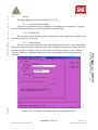
To check whether you installed the program properly, click on Tools again. The “Spatial
Analysis 1.0” option should be listed at the bottom of the Tools menu as shown in Figure ATT2.1.
Attachment 2 Page 1
Contract Number DACA05-00-D-0003
Version 1, Rev 2
Draft OESAP, September 2001
1
2
3
4
5
6
7
8
9
10
11
12
13
14
15
16
17
18
Figure ATT-2.1 Tools Menu Indicating Spatial Analysis Add-In
3.0
Operation of the Spatial Analysis Software Module
The following steps must be followed each time the spatial analysis software is used.
(1) Open Excel.
(2) Open the data file or create your own. Section 4.1 includes details about the data file
format.
(3) Select the “Spatial Analysis 1.0” option under the Tools menu to start the program.
The dialog box in Figure ATT-2.2 will appear. This box indicates the title of the
program and that it is intended for use as part of the Fort Ord OE Sampling and
Analysis Plan.
Figure ATT-2.2 Spatial Analysis Initial Dialogue Box.
Attachment 2 Page 2
Contract Number DACA05-00-D-0003
Version 1, Rev 2
Draft OESAP, September 2001
1
2
3
4
5
6
7
8
(4) Click OK to continue.
(5) Select the appropriate options under the input and output tabs, as described in section
4.0.
(6) Click the Run button. The program may require several minutes to complete analysis.
4.0
Spatial Analysis Process
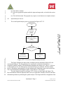
The overall spatial analysis process is presented in Figure ATT-2.3.
Start
X and Y
coordinates
of the event
and Site
Bounda ry
Estimate the e mpirical
distribution a nd compare to
complete spatia l distribution
(CSR)
(see boxes below)
Is the sec tor
Homogeneous?
Yes
Proceed with
Conc lusions and
Recommendations
9
10
11
12
13
14
15
16
17
18
19
20
No
Revisit Sector
Deve lop ment for the
site.
Figure ATT 2.3. Overview of Spatial Analysis Process
This figure illustrates the input of the coordinates and site boundaries followed by the
actual spatial analysis. The first question to be considered is whether the data follow a
completely spatially random (CSR) distribution throughout the sample area. That is, a CSR site
is a homogeneous site. Site homogeneity is determined using two methods. The first method
involves simulating a homogeneous site and comparing the simulation results to the actual data.
The second method uses the Hopkins statistic (see Section 4.1.8 for details).
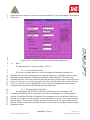
The main Spatial Analysis box (Figure ATT-2.4) has two tabs: Input and Output. The
boxes and buttons under the Input tab allow choices for input data, boundary selection, and other
information pertinent to performing the spatial analysis. The Output tab allows designation of the
Attachment 2 Page 3
Contract Number DACA05-00-D-0003
Version 1, Rev 2
Draft OESAP, September 2001
1
2
output location (worksheet or elsewhere on the current sheet). Each of the options is described in
detail below.
3
4
5
Figure ATT-2.4 Spatial Point Pattern Analysis input dialogue box.
6
7
4.1
Input
The input dialog box is shown in Figure ATT-2.4.
8
9
10
11
12
13
14
15
4.1.1 Event Coordinate Data
The Event Coordinate Data box is used to designate the location of the data to be
analyzed. The data must be organized in two adjacent columns (x, y) and there must be empty
lines and rows separating the coordinate data from any other filled cells. To set the event
coordinate data box, click once in the box, then find your data. The data can be selected in one of
two ways. The first is to just select the upper left corner cell of the data. This is shown in Figure
ATT-2.4. The other way is to highlight the area by clicking and dragging the mouse pointer
starting from the upper left corner through the lower right corner.
16
17
18
19
20
21
22
23
4.1.2 Rectangular Site Check Box
The Rectangular Site check box should be checked if the site is rectangular. The
coordinates should be listed in counterclockwise order surrounding the site, starting with the
smallest x-coordinate (Easting). Calculations for a rectangular site are much faster if this box is
checked. Five points are used to describe a four-cornered box in order to “close” the description
of the boundary. The last point should be the same as the first point. The data should be in two
adjacent columns with at least one blank column or row between the coordinate columns and the
boundary columns.
Attachment 2 Page 4
Contract Number DACA05-00-D-0003
Version 1, Rev 2
Draft OESAP, September 2001
1
2
3
4
5
6
7
8
4.1.3 Boundary Coordinate Data
The coordinates of the boundary of the sample area are input here in a counterclockwise
direction, starting with the smallest x-coordinate (Easting). As with the Event Coordinate Data,
the upper left cell of the boundary can be selected (Figure ATT-2.4). Alternatively, all points
defining the polygon boundary of the site may be selected. Either way, the coordinates should be
listed in counterclockwise order. The first and last pairs of coordinates should be the same,
producing a closed polygon. The data should be in two adjacent columns with at least one blank
column or row between the coordinate columns and the boundary columns.
9
10
11
12
13
14
15
4.1.4 Number of Simulations
This parameter refers to the number of simulations executed in order to establish the
average Empirical Distribution Function (EDF). Each simulation involves randomly distributing
events within the site and calculating the Inter-Event, Nearest Neighbor, or Point-to-NearestNeighbor distances. For test data (and faster running times), this number can be as low as 30.
However for an analysis of real data, this parameter should be set near 100. Note that the higher
the number, the longer the execution time.
16
17
18
19
4.1.5 Number of Points
This parameter is used to designate the number of points used to calculate the EDF. The
higher the number of points along this line, the smoother the resulting curve. However, there is a
corresponding increase in the execution time. This parameter should not be set to less than 20.
20
21
22
23
24
25
26
4.1.6 Coordinate Units List
This list allows the density to be reported as items per acre, hectare, and square unit
depending on the units of the input dataset coordinates.
Input
Output
Feet
items per acre
Meters
items per hectares
User Defined
items per square unit
27
28
29
30
4.1.7 Analysis and Estimation Check Boxes
The check boxes labeled “Analysis” and “Estimation” enable the spatial analysis and
density estimation options. The density estimation module calculates the density and Hopkins
Statistic. The spatial analyses and density estimation modules are discussed in more detail below.
31
32
33
34
35
36
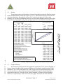
4.1.8 Types of Spatial Analyses
The program tests the data for homogeneity using Inter-Event, Nearest Neighbor, or
Point-to-Nearest-Neighbor distances. The simulation model generates the appropriate graph to
compare the data to the maximum and minimum CSR distributions (refer to boxes at end of this
manual for details). The three types of spatial analyses, Inter-Event, Nearest Neighbor, and
Point-to-Nearest-Neighbor are described in the following boxes.
Attachment 2 Page 5
Contract Number DACA05-00-D-0003
Version 1, Rev 2
Draft OESAP, September 2001
Inter-event Distance Simulation:
n(n − 1)
2
1.
For n events, calculate the
pairs of inter-event distances
2.
Calculate the empirical distribution function for the inter-event distances that can be determined for a given value
of (t) as:
# (tij ≤ t )
Hˆ 1 (t ) =
1
n(n − 1)
2
Where,
t
= A given inter-event distance,
Hˆ 1 (t )
= Empirical distribution of an inter-event distance,
= the number of inter-event distances that are less than or equal to (t), and
#(tij ≤ t)
n
= Number of event observed within the site of interest.
3.
Compare the empirical distribution to the distribution of the inter-event distances by running Monte Carlo
simulations. For each simulation, generate n events that are uniformly distributed within the area of interest,
calculate the empirical distribution function (as it was done in step 1). Then calculate the average of the all the
simulations as follows (as an approximation for the theoretical distribution function):
Hi ( t ) =
∑ Hˆ ( t )
i≠ j
( s −1)
Where,
Hi ( t )
s
= The average of Monte Carlo simulations,
= Number of Monte Carlo simulation runs.
From the simulations, also estimate the upper U(t) and the lower L(t) bounds of the distribution function as
follows:
U ( t ) = max { Hˆ i ( t ) };
L( t ) = min
i =1 ,2 ,L,s
i =1 ,2 ,L,s
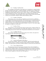
3.
Plot
Hi ( t )
on the x-axis with
(homogeneous site) the plot of
{ Hˆ ( t ) }
i
Hˆ 1 (t ),U (t ), and L(t ) on the y-axis. If the data set is uniformly distributed
H ( t ) and Hˆ (t ) will be close to 45-degree line and within the upper and lower
i
1
bounds. As shown below.
1
0.9
0.8
0.7
H(t)
0.6
0.5
0.4
0.3
0.2
0.1
0
0
0.1
0.2
0.3
0.4
0.5
0.6
0.7
0.8
0.9
1
H(t)
1
Attachment 2 Page 6
Contract Number DACA05-00-D-0003
Version 1, Rev 2
Draft OESAP, September 2001
1
Nearest Neighbor Distance Simulation:
1.
2.
For n events, calculate the n nearest neighbor distances
Calculate the empirical distribution function for the nearest neighbor distances that can be determined for a given
value of (t) as:
# (y i ≤ y )
Gˆ 1 ( y ) =
n
2.
Where,
y
= A given nearest neighbor distances,
Gˆ1 ( y )
= Empirical distribution of an nearest neighbor distances,
#(yj ≤ y)
= the number of nearest neighbor distances that are less than or equal to (y), and
n
= Number of event observed within the site of interest.
Compare the empirical distribution to the distribution of the nearest neighbor distances by running Monte Carlo
simulations. For each simulation, generate n events that are uniformly distributed within the area of interest,
calculate the empirical distribution function (as it was done in step 1). Then calculate the average of the all the
simulations as follows (as an approximation for the theoretical distribution function):
s
G1 ( y ) =
∑Gˆ ( y )
i
1
s
Where,
Gi ( y )
= The average of Monte Carlo simulations,
s
= Number of Monte Carlo simulation runs.
From the simulations, also estimate the upper U(y) and the lower L(y) bounds of the distribution function as
follows:
{
}
U ( y ) = max Gˆ i ( y ) ;
i =1, 2 ,L,s
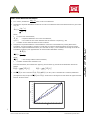
2.
i =1, 2 ,L,s
}
Gˆ1 ( y ),U ( y ), and L( y ) on the y-axis. If the data set is uniformly distributed
ˆ ( y ) will be close to 45-degree line and within the upper and
(homogeneous site) the plot of G ( y ) and G
Plot
Gˆ1 ( y )
{
L( y ) = min Gˆ i ( y )
on the x-axis with
i
1
lower bounds. As shown below.
1
0.9
0.8
0.7
G(x)
0.6
0.5
0.4
0.3
0.2
0.1
0
0
0.1 0.2 0.3 0.4 0.5 0.6 0.7 0.8 0.9
1
G(x)
Attachment 2 Page 7
Contract Number DACA05-00-D-0003
Version 1, Rev 2
Draft OESAP, September 2001
Point-to-Nearest Neighbor Distance Simulation:
1.
2.
3.
Generate m points in a regular grid KxK such that K ≈ √n.
For m points (generated randomly), calculate the m point-to-nearest event distances.
Calculate the empirical distribution function for the point-to-nearest event distances that can be determined for
a given value of (t) as:
# (x i ≤ x )
Fˆ1 ( x ) =
m
3.
Where,
x
= A given inter-event distance,
Fˆ1 ( x)
= Empirical distribution of an point-to-nearest event distances,
= the number of point-to-nearest event distances that are less than or equal to (x), and
#(xj ≤ x)
m
= Number of event observed within the site of interest.
Compare the empirical distribution to the distribution of the point-to-nearest event distances by running Monte
Carlo simulations. For each simulation, generate n events that are uniformly distributed within the area of
interest, calculate the empirical distribution function (as it was done in step 1). Then calculate the average of
the all the simulations as follows (as an approximation for the theoretical distribution function):
s
F1 ( x ) =
∑ Fˆ ( x )
i
1
s
Where,
Fi ( x )
= The average of Monte Carlo simulations,
s
= Number of Monte Carlo simulation runs.
From the simulations, also estimate the upper U(x) and the lower L(x) bounds of the distribution function as
follows:
U ( x ) = max { Fˆ i ( x ) };
L( x ) = min
i =1 ,2 ,L,s
i =1 ,2 ,L,s
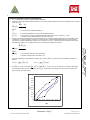
3.
Plot
Fi ( x )
on the x-axis with
(homogeneous site) the plot of
{ Fˆ ( x ) }
i
Fˆ1 ( x),U ( x), and L( x) on the y-axis. If the data set is uniformly distributed
F ( x ) and Fˆ ( x) will be close to 45-degree line and within the upper and
i
1
lower bounds. As shown below.
1
0.9
0.8
0.7
0.6
0.5
0.4
0.3
0.2
0.1
0
0
0.1 0.2 0.3 0.4 0.5 0.6 0.7 0.8 0.9 1
F(x)
1
Attachment 2 Page 8
Contract Number DACA05-00-D-0003
Version 1, Rev 2
Draft OESAP, September 2001
1
2
3
4
5
6
7
8
9
10
11
12
13
14
15
16
17
18
19
20
21
22
23
24
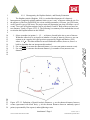
4.1.9 Homogeneity, the Hopkins Statistic, and Density Estimation
The Hopkins statistic (Hopkins, 1954) is a method that determines if a dataset is
homogeneous (completely spatially random) relative to an “event” of interest within the site. For
the purposes of the Fort Ord OESAP, the events could be anomalies, OE items, just UXO items,
or only specific types of OE items. The project team will determine just what will define a set of
events. Two types of Hopkins statistics can be calculated, H and H1. Both of these are based on
two distances, xi and yi (Figure ATT 2.5). The following is a summary of the method that is used
to calculate the Hopkins statistic in this OESAP.
1. Select at random (m) points (i = 1,2,…, m) that are located in the site or area of interest.
Within the software m is set equal to n (number of events of interest). However, one can
estimate m in a regular (kxk) grid system as proposed by Diggle and Matérn (1981)
where, k ≈ n . This latter method is not used within the software, however, there is a
built-in algorithm that can incorporate this method.
2. For each point (i) measure the shortest distance (xi) to an event (point-to nearest event).
3. For each event (i) measure the shortest distance (yi) to another event (nearest event
distance).
Figure ATT-2.5. Definition of Spatial Analysis Distances: yi are the shortest distances between
events (represented with black dots); xi are the shortest distances between randomly spaced
points (represented by blue squares) and neighboring events.
Attachment 2 Page 9
Contract Number DACA05-00-D-0003
Version 1, Rev 2
Draft OESAP, September 2001
1
2
3
4. Compute one of the following statistics:
m
H=
2
i
∑y
2
i
i =1
m
i =1
4
, or
m
H1 =
5
6
7
8
9
10
11
12
13
14
15
16
17
18
19
20
21
22
23
24
∑x
∑x
i =1
2
i
m
m
i =1
i =1
∑ yi2 + ∑ xi2
Where,
H
H1
xi
yi
= Hopkins statistic
= an alternate form of Hopkins statistic
= distance from a point i to the nearest event
= distance from an event to the next nearest event
The algorithm calculates the Hopkins statistic based on the all events available. Distance
x could be considered to represent a circular area that is empty (x is the radius of the circle).
Distance y would then represent the radius of a circular area that has an event within it. When the
Hopkins statistic is large, it indicates that the site is not homogeneous and when it is small, the
area under investigation can be considered homogeneous. Note that Hopkins in his paper defined
the statistic in H1 form. Diggle (1983) used the H form of Hopkins statistic.
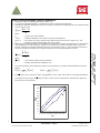
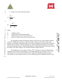
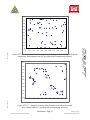
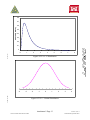
The distribution of events (data) in Figure ATT-2.6 illustrates a relatively homogeneous
distribution. If the site has clustered data (i.e. is not homogeneous), as in Figure ATT-2.7, you
would expect to see larger areas (patches) that are empty. This distribution results in large x
values relative to the y distances because of event clustering and so the Hopkins statistic is large.
Attachment 2 Page 10
Contract Number DACA05-00-D-0003
Version 1, Rev 2
Draft OESAP, September 2001
1
0.9
0.8
0.7
0.6
0.5
0.4
0.3
0.2
0.1
0
0
1
2
3
4
0.1
0.2
0.3
0.4
0.5
0.6
0.7
0.8
0.9
1
Figure ATT-2.6 – Example of events considered to be homogeneously distributed (from the
sample data “homogeneous data.xls” provided with accompanying software)
1.0
0.9
0.8
0.7
0.6
0.5
0.4
0.3
0.2
0.1
0.0
0.0
5
6
7
8
0.1
0.2
0.3
0.4
0.5
0.6
0.7
0.8
0.9
1.0
Figure ATT-2.7 – Example of an area with clustered events (from the sample
data “clustered data.xls” provided with accompanying software).
Attachment 2 Page 11
Contract Number DACA05-00-D-0003
Version 1, Rev 2
Draft OESAP, September 2001
1
2
3
4
5
6
7
8
9
10
11
12
13
14
15
16
17
18
19
20
21
22
23
24
25
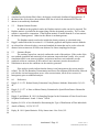
Statistically, H follows an F-distribution. This distribution arises from a ratio between
two sums of squares each of which has its own degrees of freedom (df). The degrees of freedom
associated with the numerator and denominator are designated as (df1 and df2), respectively.
These two parameters define a specific F-distribution (Figure ATT-2.8). H follows an Fdistribution with both degrees of freedom equal to m. H1 follows a beta distribution BETA(m,m).
Note that a beta distribution is defined by two parameters. The software uses the beta
distribution. However, H1 follows a normal distribution (Figure ATT-2.9) with a mean of 0.5 and
−1
variance of (4(2m + 1)) when the number of events n is large (n > 50). The accompanying
spatial analysis software module (Spatial Analysis Ver. 1.0) calculates the Hopkins statistic. The
calculated H value can be compared to the computed F-distribution value to objectively
determine whether it is large enough. If H > F, then the site is not homogeneous. Otherwise, the
site is considered homogeneous. The same logic applies with the H1 statistic compared to the
appropriate value from a beta distribution.
There are several methods to estimate the density of an event. Two methods are outlined
here. The first method is based on the estimate of a Poisson process and is applicable to sites that
are CSR. The density λ is estimated using the following equation (from Ripley, 1981):


~  m
λ =
 m
 2∑ x i
 i =1






2
This estimate can be generalized if we look for k nearest events from each point. In this
case, xi represents the smallest distance from point i that contains k events. That is, the density
estimate can be represented by:
mk
λˆ =
m
π ∑ xi2
i =1
26
27
28
29
30
31
32
33
The other method (Diggle, 1975 and 1977) involves two measurements: Point-to-Nearest
event and event-to-nearest event (i.e. Nearest Neighbor) distances. This method is more
appropriate for areas that are not CSR. The density is estimated as follows:
m
λ* =
1
 m 2 m 2 2
π  ∑ xi ∑ y i 
 i =1 i =1 
The attached software uses Diggle’s method to estimate the density.
Attachment 2 Page 12
Contract Number DACA05-00-D-0003
Version 1, Rev 2
Draft OESAP, September 2001
0.8
0.7
Probability Density
0.6
0.5
0.4
0.3
0.2
0.1
0
0
1
2
1
2
3
3
4
5
6
7
8
Figure ATT-2.8 – F Distribution
-4
-3
4
5
6
7
-2
-1
0
1
2
3
4
Figure ATT-2.9 – Normal Distribution
Attachment 2 Page 13
Contract Number DACA05-00-D-0003
Version 1, Rev 2
Draft OESAP, September 2001
1
2
4.2
Output
The output dialog box is shown in Figure ATT-2.10.
3
4
5
4.2.1 Screen Update Check Box
If this box is checked the screen is updated as the simulations are completed. Updating
the screen during program execution slows the process significantly.
6
7
8
4.2.2 Problem Title
The text entered in the Problem Title area will appear on the output above the EDF data if
the analysis check box is checked.
9
10
11
12
13
14
4.2.3 Output Options
The user can select the output location in the Output Options section. If the Range radio
button is selected, the output will appear in the same worksheet as the dataset, starting at the cell
location specified. Alternatively the user can choose to direct the output to a new worksheet.
The name of the new worksheet cannot be the same as an existing worksheet in the current
workbook.
15
16
17
Figure ATT-2.10 Spatial Point Pattern Analysis output dialogue box.
Attachment 2 Page 14
Contract Number DACA05-00-D-0003
Version 1, Rev 2
Draft OESAP, September 2001
1
2
3
4
5
6
7
5.0
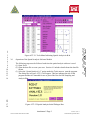
Results
The program output can include three sections, the graphical results, the Hopkins statistic
results, and the summary conclusion (Figure ATT 2.11). If the analysis check box was selected
in the input dialog box the graphical results will be located in the upper left of the output
worksheet. If the Density Estimation check box was selected the Hopkins statistic results will be
located below the graphical results. The summary report box is located below the other results.
Cluttered Data Inter-Event Analysis
Inter-event Distance Matrix
Events
Data EDF
Inter-Event Distance Simulations
Data
CSR**
Distance
EDF*
EDF
CSR Min CSR Max
0
0
0
0
0
0.053187 0.02697 0.008662 0.004231 0.013749
0.106374 0.074564 0.031787 0.021682 0.048123
0.15956 0.118985 0.069154 0.056584 0.09413
0.212747 0.152829
0.1177 0.097832 0.140137
0.265934 0.197779 0.174802 0.144368 0.225806
0.319121 0.254892 0.239937 0.182443 0.304072
0.372307 0.331042 0.307144 0.268641 0.364886
0.425494 0.432047 0.374696 0.301957 0.459016
0.478681 0.504495 0.456579 0.389212 0.548387
0.531868 0.567953 0.530873 0.462718 0.625595
0.585054 0.635114 0.595923 0.50238 0.720783
0.638241 0.69487 0.65771 0.566367 0.740878
0.691428 0.758329 0.741211 0.635114 0.838181
0.744615 0.817557 0.793321 0.69963 0.881015
0.797802 0.892121 0.849149 0.750925 0.920148
0.850988 0.936542 0.892993 0.819672 0.964569
0.904175 0.969857 0.930915 0.890005 0.966684
0.957362 0.990481 0.960999 0.925436 0.988366
1.010549 0.998942 0.978001 0.95082 0.995769
* Empirical Distribution Function
** Complete Spatial Randomness
0.486311 Mean of Inter-Event Distance
0.241512 Standrad deviation of Inter-Event Distance
Density Estimate
4.39E+01 2.5% Percentile Items/unit area
5.53E+01 Average density Items/unit area
6.89E+01 97.5% Percentile Items/unit area
Hopkins (H) Statistic
2.706
4.24
7.09
1.424
2.5% Percentile
Median
97.5% Percentile
F-Statistic
1
0.9
0.8
0.7
0.6
0.5
0.4
0.3
0.2
0.1
0
0
0
0.534 0.509513
0.534
0 0.10373
0.509513 0.10373
0
0.757024 0.46401 0.375133
0.960417 0.820705
0.722
Cluttered Data Inter-Event
Analysis
0.405216
0.324746 0.231491
0.533622 0.651659 0.554274
0.601881 0.721336 0.622274
0.754414 0.938614 0.840215
0.747533 0.846681 0.744823
0.366175 0.780605 0.71342
0.471349 0.824181 0.745618
0.492306 0.847127 0.768118
0.119
0.415 0.393402
0.53424
0.016 0.088769
0.418016 0.12492 0.101514
0.858336
0.672 0.575006
0.904613 0.833969 0.731579
0.1 0.2 0.3 0.4 0.5
0.6 0.7
0.8 0.90.241249
1
0.342358
0.321442
0.617408 0.519766
CSR0.517673
EDF
0.727396 0.983897 0.890484
0.754192 0.914224 0.814632
0.698216 0.803473 0.702325
0.379812 0.775475 0.705292
0.557412 0.935778 0.857834
0.507256 0.855902 0.775766
0.078645 0.45728 0.430875
0.475
0.059 0.101139
0.424005 0.143694 0.08551
0.878046
0.697 0.599964
0.354249 0.274401 0.197363
0.359388 0.389343 0.302344
0.539356 0.583123 0.48278
0.767628 1.014002 0.919278
**** Summary Report ****
5.53E+01 Average Density Items/unit area
The site is not homogeneous based the Hopkins test statistic
Based on the EDF graph, the site is not homogeneous
8
9
10
11
12
13
14
15
16
0.7712 0.913226 0.81267
0.687255 0.776971 0.675435
0.403565 0.775766 0.701838
0.549626 0.92136 0.84277
Figure ATT 2.11. Example output from both graphical and Hopkins statistic analysis.
5.1
Graphical Results
The simulation model generates the appropriate graph (Inter-Event, Nearest-Neighbor, or
Point-to-Nearest Neighbor) that compares the dataset to a completely spatially random (CSR)
distribution. The x axis of this graph is the CSR average empirical distribution function (EDF)
from the simulations. The maximum and minimum EDFs are plotted as dashed black lines
against the average EDF. The Inter-Event, Nearest-Neighbor, or Point-to Nearest-Neighbor
distances are represented by a blue line on the same graph. If that blue line falls within the
Attachment 2 Page 15
Contract Number DACA05-00-D-0003
Version 1, Rev 2
Draft OESAP, September 2001
1
2
3
simulated envelop (dashed black lines), the dataset is uniformly distributed (homogeneous). If
the dataset line crosses above the maximum EDF line or below the minimum EDF line the
dataset is not uniformly distributed.
4
5
6
7
8
9
10
11
12
13
5.2
Hopkins Statistic Results
In addition to the graphical results, the Hopkins statistic results can also be reported. The
Hopkins statistic is included in the output along with the designated percentiles. The F or beta
statistic is reported for comparison. If the Hopkins statistic is smaller than the F or beta statistic
the dataset is homogeneous. Otherwise the dataset is not homogeneous.
14
15
16
17
18
19
20
21
22
23
24
25
26
27
28
29
30
31
32
33
34
35
36
37
38
39
40
5.3
The Hopkins statistic results also include the density estimate, as calculated using
Diggle’s method described in section 4.1.9. If both the graphical and Hopkins statistic methods
are selected the software displays a mean and standard deviation that can be used to select the
distance between transects or buffer zone distance for future sampling plan designs.
Summary Report
The summary report box concisely outlines the result of the analyses. If the results of the
two methods (graphical and statistical) are inconsistent, inspect the data visually. Also, run all
simulations (inter-event, nearest neighbor, and point-to-nearest event) and make sure the
graphical results are consistent. If the results are not consistent, increase the number of
simulations to increase the confidence in the statistics generated.
If the analysis results indicate that the dataset is not homogeneous the sectors must be
refined. The OE Site Boundary Determination and Sector Development SOP should be followed
to divide the site into homogeneous areas. After resectorization, check all new sectors for
homogeneity prior to additional analysis.
6.0
References
Diggle, P. J. 1975. Robust Density Estimation Using Distance Methods. Biometrika. 62(1):3948.
Diggle, P. J. 1977. A Note on Robust Density Estimation for Spatial Point Pattern. Biometrika.
64(1):91-95.
Diggle, P. and Matern, B. 1981. On Sampling Designs for the Estimation of Point-Event Nearest
Neighbor Distributions. Scand. J. Statist. 7:80-84.
Hopkins, B. 1954. A New Method for Determining the Type of Distribution of Plant Individuals.
Annals of Botany. 18 (70) 213:227.
Ripley, B. 1981. Spatial Statistics. Wiley Interscience. New York, NY.
Attachment 2 Page 16
Contract Number DACA05-00-D-0003
Version 1, Rev 2
Draft OESAP, September 2001
1
2
3
4
5
6
7
8
9
10
11
12
13
14
15
16
17
18
19
20
21
22
23
24
25
26
27
28
29
30
31
32
33
34
35
36
37
38
39
40
41
42
43
44
45
46
47
48
49
50
51
52
53
54
55
56
57
58
59
60
61
62
63
64
65
66
7.0
Program Listing
Public distance(1 To 1000, 1 To 1000), Point(1 To 200, 1 To 2)
Public PEdistance(1 To 1000, 1 To 1000), PEDistanceRange As Range, iPlist(1 To 1000)
Public XE As Range, BRange As Range, NBPoints As Integer
Public BB As Range, Y(1 To 50), D(1 To 50)
Public add1, iList(1 To 1000), distf(1 To 1000)
Public n As Integer, Pline(1 To 100)
Public onsite As Boolean
Public Bline(1 To 1000, 1 To 4), Oldsheet
Public DistanceRange As Range, YO As Range
Public Xcoor(1 To 1000), Ycoor(1 To 1000), ResultsSheet
Public xminb, xmaxb, yminb, ymaxb, starttime
Public OldName, EDfData(1 To 1000), AnalysisTitle$, outputAddress, EDfDatax(1 To 1000)
Public ybar(1 To 1000) As Single, EDFMin(1 To 1000) As Single, EDFMax(1 To 1000) As Single
Public Ndistances, Nsimulations, m As Integer
Public EXCoor(1 To 1000), EYCoor(1 To 1000), Standard_Deviation, Distance_Mean
Public DataWorkbook As Workbook, IsItCSR As Boolean, steep As Boolean
Public NewWorkbook, NBreakPoints As Integer, BoderPoints As Integer
Sub RunPPA()
SpatialPoint.LabelProgress.Width = 0
Load Logo
Logo.Show
End Sub
Sub InitialSetup()
With SpatialPoint
.OK.Enabled = False
.Cancel.Enabled = False
.LabelHelpInput.BackColor = &HFF&
.LabelHelpInput.Caption = _
"In order to stop the program press Ctrl-Break and then push End"
End With
starttime = Timer
Set Oldsheet = ActiveSheet
OldName = Oldsheet.Name
Set DataWorkbook = ActiveWorkbook
DataBookName = DataWorkbook.Name
'
' This part determines where to show the output
'
If SpatialPoint.BtnOutputRange.Value Then
outputAddress = Range(SpatialPoint.RefOutputRange.Value).Address
Cn = Range(outputAddress).Column
Rn = Range(outputAddress).Row
Range(outputAddress & ":" & Range(outputAddress).Offset(65535 - Rn, _
256 - Cn).Address).Cells.Clear
Set ResultsSheet = ActiveSheet
NewWorkbook = ActiveWorkbook.Name
End If
'
' This part determines if the sheet name entered exits
'
If SpatialPoint.BtnNewWorksheet.Value Then
newname = SpatialPoint.TbxNewWorksheet.Value
Attachment 2 Page 17
Contract Number DACA05-00-D-0003
Version 1, Rev 2
Draft OESAP, September 2001
1
2
3
4
5
6
7
8
9
10
11
12
13
14
15
16
17
18
19
20
21
22
23
24
25
26
27
28
29
30
31
32
33
34
35
36
37
38
39
40
41
42
43
44
45
46
47
48
49
50
51
52
53
54
55
56
57
58
59
60
61
62
63
64
65
66
67
NewSheet = True
Do While NewSheet
For Each Item In ActiveWorkbook.Sheets
If Item.Name = newname Then
MsgBox "The Sheet name " & newname & " you entered already exit!"
newname = InputBox("Enter a new name")
Else
NewSheet = False
End If
Next Item
Loop
Set ResultsSheet = Sheets.Add
ResultsSheet.Name = newname
NewWorkbook = ActiveWorkbook.Name
outputAddress = Range("A1").Address
End If
'
' This part handles adding a new workbook for the output
'
If SpatialPoint.BtnNewWorkbook.Value Then
outputfile = SpatialPoint.tbxFileLocation.Value & SpatialPoint.TbxNewWorkbook.Value
Workbooks.Add
ActiveWorkbook.SaveAs FileName:=outputfile & ".xls", FileFormat:=xlNormal, _
Password:="", WriteResPassword:="", ReadOnlyRecommended:=False _
, CreateBackup:=False
Set ResultsSheet = ActiveSheet
outputAddress = "A1"
NewWorkbook = SpatialPoint.TbxNewWorkbook.Value & ".xls"
End If
Windows(NewWorkbook).Activate
Oldsheet.Activate
Set XE = Range(SpatialPoint.EventCoordinates.Value).CurrentRegion
n = XE.Rows.Count
For i = 1 To n
EXCoor(i) = XE.Cells(i, 1).Value
EYCoor(i) = XE.Cells(i, 2).Value
Next i
Set BRange = Range(SpatialPoint.BoundaryLine.Value).CurrentRegion
NBPoints = BRange.Rows.Count
xminb = Application.WorksheetFunction.Min(BRange.Columns(1).Value)
xmaxb = Application.WorksheetFunction.Max(BRange.Columns(1).Value)
yminb = Application.WorksheetFunction.Min(BRange.Columns(2).Value)
ymaxb = Application.WorksheetFunction.Max(BRange.Columns(2).Value)
'
' This part determines if the site is rectagular. Calculations are less
' involved when the site is rectangualr.
'
If Not SpatialPoint.Rectangle Then
add1 = BRange.Cells(1, 1).Address
add2 = Range(add1).Offset(NBPoints - 1, 3).Address
Set BRange = Range(add1, add2)
For i = 1 To NBPoints
Bline(i, 1) = BRange.Cells(i, 1).Value
Attachment 2 Page 18
Contract Number DACA05-00-D-0003
Version 1, Rev 2
Draft OESAP, September 2001
1
2
3
4
5
6
7
8
9
10
11
12
13
14
15
16
17
18
19
20
21
22
23
24
25
26
27
28
29
30
31
32
33
34
35
36
37
38
39
40
41
42
43
44
45
46
47
48
49
50
51
52
53
54
55
56
57
58
59
60
61
62
63
64
65
66
67
Bline(i, 2) = BRange.Cells(i, 2).Value
Bline(i, 3) = Sqr(Bline(i, 1) ^ 2 + Bline(i, 2) ^ 2)
If Bline(i, 2) = 0 Then
Bline(i, 4) = Atn(1) * 2
' pi/2
Else
Bline(i, 4) = Atn(Bline(i, 1) / Bline(i, 2))
End If
Next i
BRange.Value = Bline
Call PrepareBoundary
End If
'XE.Activate
If SpatialPoint.chkanalysis Then
If SpatialPoint.InterEvent Then
AnalysisTitle = "Inter-Event Distance "
Call TitleSetup(outputAddress)
Call IE_Main
Call EDFPlot
Call CheckPlot
ElseIf SpatialPoint.NearestNeighbor Then
NNB = 1
AnalysisTitle = "Nearest Neighbor Distance "
Call TitleSetup(outputAddress)
Call NN_Main
Call EDFPlot
Call CheckPlot
ElseIf SpatialPoint.PointNearestEvent Then
PNE = 1
AnalysisTitle = "Point-to-Nearest Event Distance "
Call TitleSetup(outputAddress)
Call PNE_Main
Call EDFPlot
Call CheckPlot
End If
'
' Delete the temporary sheet without alerting the user
' for deleting the sheet.
'
Application.DisplayAlerts = False
Sheets("Temp1").Delete
Application.DisplayAlerts = True
End If
If SpatialPoint.btnDensity Then
'If NNB = 0 Then
' Call InterEventDistance
' Set DistanceRange = Oldsheet.Range("I1" & ":" & Range("I1").Offset(n - 1, _
'
n - 1).Address)
' DistanceRange.Value = distance
' Call nearest
'End If
Attachment 2 Page 19
Contract Number DACA05-00-D-0003
Version 1, Rev 2
Draft OESAP, September 2001
1
2
3
4
5
6
7
8
9
10
11
12
13
14
15
16
17
18
19
20
21
22
23
24
25
26
27
28
29
30
31
32
33
34
35
36
37
38
39
40
41
42
43
44
45
46
47
48
49
50
51
52
53
54
55
56
57
58
59
60
61
62
63
64
65
66
67
Call DensityEstimate
End If
SpatialPoint.LabelProgressTitle.Caption = "Total time was " & _
Format((Timer - starttime) / 60, "0.0") & " minutes"
With SpatialPoint
.Cancel.Caption = "Close"
.Cancel.Enabled = True
End With
End Sub
Function MinifLoca(List) As Integer
' This function finds the minimum element such that
' it subject to a condition
'
xmin = Application.WorksheetFunction.Min(List)
'MinifLoca = Application.WorksheetFunction.Match(xmin, List, 0)
End Function
Sub InterEventDistance()
'
' In this procedure the distances between events
' XE is the event coordinates
' n is the number of events
' Generate the upper triangle
'
' Set XE = Range(SpatialPoint.EventCoordinates.Value)
' This line was deleted to accomodate the simulation
'
'n = XE.Rows.Count
For i = 1 To n
distance(i, i) = 0
Next i
sumied = 0
For i = 1 To n
For j = i + 1 To n
delx = XE.Cells(i, 1) - XE.Cells(j, 1)
dely = XE.Cells(i, 2) - XE.Cells(j, 2)
distance(i, j) = Sqr(delx * delx + dely * dely)
sumied = sumied + distance(i, j)
distance(j, i) = distance(i, j)
Next j
Next i
End Sub
Sub nearest()
'
' This procedure calculates the iList vector that list the
' nearest neighbor to event 1 through n.
' The nearest distance can be accessed by Distance(i, iList(i))
' Note: iList is a row vector as far VB is concerned. So it needs
' to be transposed if it is printed to a column within the spreadsheet.
'
Dim theRange As Range, xx As Range
'
' Set XE = Range(SpatialPoint.EventCoordinates.Value)
' See intereventdistance module for justification
Attachment 2 Page 20
Contract Number DACA05-00-D-0003
Version 1, Rev 2
Draft OESAP, September 2001
1
2
3
4
5
6
7
8
9
10
11
12
13
14
15
16
17
18
19
20
21
22
23
24
25
26
27
28
29
30
31
32
33
34
35
36
37
38
39
40
41
42
43
44
45
46
47
48
49
50
51
52
53
54
55
56
57
58
59
60
61
62
63
64
65
66
67
'
'n = XE.Rows.Count
For i = 1 To n
If i = 1 Then ' Need to exclude the zeros along the diagonal
Set xx = Range(DistanceRange.Cells(1, 2).Address & _
":" & DistanceRange.Cells(1, n).Address)
'xmin = Application.WorksheetFunction.Min(xx)
ElseIf i = n Then
Set xx = Range(DistanceRange.Cells(n, 1).Address & _
":" & DistanceRange.Cells(n, n - 1).Address)
'xmin = Application.WorksheetFunction.Min(xx)
Else
x1 = DistanceRange.Cells(i, 1).Address & _
":" & DistanceRange.Cells(i, i - 1).Address
X2 = DistanceRange.Cells(i, i + 1).Address & _
":" & DistanceRange.Cells(i, n).Address
Set xx = Union(Range(x1), Range(X2))
End If
xmin = Application.WorksheetFunction.Min(xx)
Set theRange = DistanceRange.Rows(i)
iList(i) = Application.WorksheetFunction.Match(xmin, _
theRange, 0)
Next i
End Sub
Sub EmpiricaDistFunction(distf, Nsize, Y, EDFy)
'
' In this procedure, the empirical distribution function is calculated
' Distf is the list of distances of interest (e.g., nearest neighbor)
' EDFy is the array that contains the values of CDF the correspond to
' the distance y
' Nsize is the size of EDF
'
EDFy = Application.WorksheetFunction.CountIf(distf _
, ">=" & Y) / Nsize
End Sub
Sub IE_Main()
Call InterEventDistance
' Generate the interEvent distances
Windows(NewWorkbook).Activate
LeftCorner = Range(outputAddress).Offset(3, 8).Address
RightCorner = Range(LeftCorner).Offset(n - 1, n - 1).Address
Set DistanceRange = ResultsSheet.Range(LeftCorner & ":" & RightCorner)
DistanceRange.Value = distance
Nsimulations = CInt(SpatialPoint.NumberSimulations.Value)
Ndistances = CInt(SpatialPoint.NumberDistances.Value)
ymax = Application.WorksheetFunction.Max(DistanceRange)
For i = 1 To n
If i = 1 Then ' Need to exclude the zeros along the diagonal
Set xx = Range(DistanceRange.Cells(1, 2).Address & _
":" & DistanceRange.Cells(1, n).Address)
ElseIf i = n Then
Set xx = Range(DistanceRange.Cells(n, 1).Address & _
":" & DistanceRange.Cells(n, n - 1).Address)
Else
x1 = DistanceRange.Cells(i, 1).Address & _
":" & DistanceRange.Cells(i, i - 1).Address
X2 = DistanceRange.Cells(i, i + 1).Address & _
":" & DistanceRange.Cells(i, n).Address
Set xx = Union(Range(x1), Range(X2))
End If
If i = 1 Then
ymin = Application.WorksheetFunction.Min(xx)
Else
Attachment 2 Page 21
Contract Number DACA05-00-D-0003
Version 1, Rev 2
Draft OESAP, September 2001
1
2
3
4
5
6
7
8
9
10
11
12
13
14
15
16
17
18
19
20
21
22
23
24
25
26
27
28
29
30
31
32
33
34
35
36
37
38
39
40
41
42
43
44
45
46
47
48
49
50
51
52
53
54
55
56
57
58
59
60
61
62
63
64
65
66
67
ymin1 = Application.WorksheetFunction.Min(xx)
If ymin1 < ymin Then
ymin = ymin1
End If
End If
Next i
yrange = ymax - ymin
For K = 1 To Ndistances
Y(K) = ymin + (K - 1) * yrange / Ndistances
EDfDatax(K) = (Application.WorksheetFunction.CountIf(DistanceRange, "<=" & Y(K)) _
- n) / 2 / (n * (n - 1) / 2)
Next K
dataAddress = Range(outputAddress).Offset(3, 0).Address
Set YO = ResultsSheet.Range(dataAddress & ":" & _
Range(dataAddress).Offset(Ndistances - 1, 0).Address)
YO.Value = Application.WorksheetFunction.Transpose(Y)
Set Yhato = ResultsSheet.Range(Range(dataAddress).Offset(0, 1).Address & ":" & _
Range(dataAddress).Offset(Ndistances - 1, 1).Address)
Yhato.Value = Application.WorksheetFunction.Transpose(EDfDatax)
Nied = (n ^ 2 - n) / 2
' Number of Inter-event distances
sumied = 0
sumiedsq = 0
For i = 1 To n
For j = i + 1 To n
sumied = sumied + distance(i, j)
sumiedsq = sumiedsq + distance(i, j) ^ 2
Next j
Next i
Distance_Mean = sumied / Nied
Standard_Deviation = Sqr((Nied * sumiedsq - sumied ^ 2) / (Nied * (Nied - 1)))
Call MonteCarloIE
End Sub
Sub NN_Main()
'
' Need to calculate the actual distribution based on the event
' Reported
'
'Oldsheet.Activate
Call InterEventDistance
Windows(NewWorkbook).Activate
ResultsSheet.Activate
LeftCorner = Range(outputAddress).Offset(3, 8).Address
RightCorner = Range(LeftCorner).Offset(n - 1, n - 1).Address
Set DistanceRange = Range(LeftCorner & ":" & RightCorner)
DistanceRange.Value = distance
Call nearest
'
' Need to calculate the expected distribution from a homogeneous
' distribution.
' These simulations are repeated Nsimulations times
' Also, the envelope of the maximum and minimum values from the
' simulations is estimated for comparison purposes.
Attachment 2 Page 22
Contract Number DACA05-00-D-0003
Version 1, Rev 2
Draft OESAP, September 2001
1
2
3
4
5
6
7
8
9
10
11
12
13
14
15
16
17
18
19
20
21
22
23
24
25
26
27
28
29
30
31
32
33
34
35
36
37
38
39
40
41
42
43
44
45
46
47
48
49
50
51
52
53
54
55
56
57
58
59
60
61
62
63
64
65
66
67
Nsimulations = CInt(SpatialPoint.NumberSimulations.Value)
Ndistances = CInt(SpatialPoint.NumberDistances.Value)
'
' Generate distance overwhich the CDF is estimated
'
For i = 1 To n
distf(i) = distance(i, iList(i))
Next i
Distance_Mean = Application.WorksheetFunction.Average(distf)
Standard_Deviation = Application.WorksheetFunction.StDev(distf)
'
' Yrange allows to guess the distances overwhich we can estimate
' the empirical distribution function
' This should be revisited for a more robust mehtod
'
ymax = Application.WorksheetFunction.Max(distf)
ymin = Application.WorksheetFunction.Min(distf)
yrange = ymax - ymin
FirstCell = ResultsSheet.Range(outputAddress).Offset(3, 6).Address
LastCell = ResultsSheet.Range(FirstCell).Offset(n - 1, 0).Address
Set EDFO = ResultsSheet.Range(FirstCell & ":" & LastCell)
EDFO.Value = Application.WorksheetFunction.Transpose(distf)
'
' Calculate the distance overwhich the empirical distribution
' is calculated y(k). Also, calculate the empirical distridution
' for the data EDFData(k).
'
For K = 1 To Ndistances
Y(K) = ymin + (K - 1) * yrange / Ndistances
EDfDatax(K) = Application.WorksheetFunction.CountIf(EDFO, "<=" _
& Y(K)) / n
Next K ' Should check the statement above countif syntax and the
' name of the array dist
dataAddress = ResultsSheet.Range(outputAddress).Offset(3, 0).Address
Set YO = ResultsSheet.Range(dataAddress & ":" & _
Range(dataAddress).Offset(Ndistances - 1, 0).Address)
YO.Value = Application.WorksheetFunction.Transpose(Y)
FirstCell = ResultsSheet.Range(dataAddress).Offset(0, 1).Address
LastCell = ResultsSheet.Range(FirstCell).Offset(Ndistances - 1, 0).Address
Set Yhato = ResultsSheet.Range(FirstCell & ":" & LastCell)
Yhato.Value = Application.WorksheetFunction.Transpose(EDfDatax)
'
'
'
'
'
'
'
'
'
'
This part runs the simulations for Nsimulations times for each
of the distances (Ndistances)
The TempSheet inserts a sheet to use for the simulation
The sheet is named "Temp1"
Later I need to add a module to make sure this is a unique
name. At this stage this is not important.
Application.ScreenUpdating = SpatialPoint.ChkScreenupdate
Call MonteCarloNB
End Sub
Attachment 2 Page 23
Contract Number DACA05-00-D-0003
Version 1, Rev 2
Draft OESAP, September 2001
1
2
3
4
5
6
7
8
9
10
11
12
13
14
15
16
17
18
19
20
21
22
23
24
25
26
27
28
29
30
31
32
33
34
35
36
37
38
39
40
41
42
43
44
45
46
47
48
49
50
51
52
53
54
55
56
57
58
59
60
61
62
63
64
65
66
67
Sub PNE_Main()
'
'
'
'
'
'
'
'
'
'
'
Need to calculate the actual distribution based on the event
Reported
For this simulation, we need to divide the site into grids
Number of grids obtained by grid = Int(N), where N is the
number of points
The center of each grid will be considered the initial point
to estimate the empirical distribution.
Then by simulation we can generate the actual distribution and envelope
of the distribution
'Oldsheet.Activate
Nsimulations = SpatialPoint.NumberSimulations.Value
Ndistances = SpatialPoint.NumberDistances.Value
'
'
'
'
'
'
'
'
'
'
'
'
grid = Int(Sqr(n))
m = grid ^ 2
Generate the x and y coordinates for the points located in the middle of each grid
For i = 1 To grid
For j = 1 To grid
K = grid * (i - 1) + j
Point(K, 1) = xminb + (j - 0.5) * (xmaxb - xminb) / grid
Point(K, 2) = yminb + (i - 0.5) * (ymaxb - yminb) / grid
Next j
Next i
m=n
Call RandomPoints(m)
For i = 1 To m
Point(i, 1) = Xcoor(i)
Point(i, 2) = Ycoor(i)
Next i
'
' Calculate the distances from the points to nearest event
'
Call PointEventDistance
Windows(NewWorkbook).Activate
PEDLeftCorner = ResultsSheet.Range(outputAddress).Offset(6 + n, 8).Address
PEDRightCorner = ResultsSheet.Range(PEDLeftCorner).Offset(n - 1, m - 1).Address
Set PEDistanceRange = ResultsSheet.Range(PEDLeftCorner & ":" & PEDRightCorner)
PEDistanceRange.Value = PEdistance
'
' Generate the nearest event to each of the points
'
For i = 1 To m
xmin = Application.WorksheetFunction.Min(PEDistanceRange.Columns(i))
Set theRange = PEDistanceRange.Columns(i)
iPlist(i) = Application.WorksheetFunction.Match(xmin, _
theRange, 0)
distf(i) = PEdistance(iPlist(i), i)
Attachment 2 Page 24
Contract Number DACA05-00-D-0003
Version 1, Rev 2
Draft OESAP, September 2001
1
2
3
4
5
6
7
8
9
10
11
12
13
14
15
16
17
18
19
20
21
22
23
24
25
26
27
28
29
30
31
32
33
34
35
36
37
38
39
40
41
42
43
44
45
46
47
48
49
50
51
52
53
54
55
56
57
58
59
60
61
62
63
64
65
66
67
Next i
Standard_Deviation = Application.WorksheetFunction.StDev(distf)
Distance_Mean = Application.WorksheetFunction.Average(distf)
FirstCell = Range(outputAddress).Offset(3, 6).Address
LastCell = Range(FirstCell).Offset(m - 1, 0).Address
Set EDFO = Range(FirstCell & ":" & LastCell)
EDFO.Value = Application.WorksheetFunction.Transpose(distf)
DMin = Application.WorksheetFunction.Min(distf)
DMax = Application.WorksheetFunction.Max(distf)
DRange = DMax - DMin
For K = 1 To Ndistances
D(K) = DMin + (K - 1) * DRange / Ndistances
EDfDatax(K) = Application.WorksheetFunction.CountIf(EDFO, "<=" & D(K)) / m
Next K
dataAddress = Range(outputAddress).Offset(3, 0).Address
Set YO = ResultsSheet.Range(dataAddress & ":" & _
Range(dataAddress).Offset(Ndistances - 1, 0).Address)
YO.Value = Application.WorksheetFunction.Transpose(D)
Set Yhato = ResultsSheet.Range(Range(dataAddress).Offset(0, 1).Address & ":" & _
Range(dataAddress).Offset(Ndistances - 1, 1).Address)
Yhato.Value = Application.WorksheetFunction.Transpose(EDfDatax)
'
'
'
'
'
'
'
'
'
'
This part runs the simulations for Nsimulations times for each
of the distances (Ndistances)
The TempSheet inserts a sheet to use for the simulation
The sheet is named "Temp1"
Later I need to add a module to make sure this is a unique
name. At this stage this is not important.
Call MonteCarloPNE
End Sub
Sub PointEventDistance()
' In this procedure the distances between events
' XE is the event coordinates
' n is the number of events
' Generate the upper triangle
Dim i As Integer, j As Integer
Dim delx As Single, dely As Single
Dim X As Single
'
' Set XE = Range(SpatialPoint.EventCoordinates.Value)
' This line was deleted to accomodate the simulation
'
For i = 1 To n
For j = 1 To m
delx = XE.Cells(i, 1) - Point(j, 1)
dely = XE.Cells(i, 2) - Point(j, 2)
PEdistance(i, j) = Sqr(delx * delx + dely * dely)
Attachment 2 Page 25
Contract Number DACA05-00-D-0003
Version 1, Rev 2
Draft OESAP, September 2001
1
2
3
4
5
6
7
8
9
10
11
12
13
14
15
16
17
18
19
20
21
22
23
24
25
26
27
28
29
30
31
32
33
34
35
36
37
38
39
40
41
42
43
44
45
46
47
48
49
50
51
52
53
54
55
56
57
58
59
60
61
62
63
64
65
66
67
Next j
Next i
End Sub
Sub PointNearest()
'
' This procedure calculates the iList vector that list the
' nearest neighbor to event 1 through n.
' The nearest distance can be accessed by Distance(i, iList(i))
' Note: iList is a row vector as far VB is concerned. So it needs
' to be transposed if it is printed to a column within the spreadsheet.
'
'
' Set XE = Range(SpatialPoint.EventCoordinates.Value)
' See intereventdistance module for justification
'
For i = 1 To m
xmin = Application.WorksheetFunction.Min(DistanceRange.Columns(i))
Set theRange = DistanceRange.Columns(i)
iPlist(i) = Application.WorksheetFunction.Match(xmin, _
theRange, 0)
Next i
End Sub
Sub RandomPoints(NPoints)
'
' Need to generate random points that fall within the boundary
' of the site
' BLine is the site border line that closes and should go
' counterclock wise.
' YmaxB, YminB, XmaxB, and XminB are the limits of a box that contains
' the site boundary
'
'Dim Xcoor(1 To 1000), Ycoor(1 To 1000)
'Dim Bline(1 To 100, 1 To 4), Pline(1 To 50) As Integer
For i = 1 To NPoints
K=1
Do While K = 1
Xcoor(i) = xminb + (xmaxb - xminb) * Rnd(Timer)
Ycoor(i) = yminb + (ymaxb - yminb) * Rnd(Timer)
'
' Check these points if they are within the site
'
If SpatialPoint.Rectangle Then
Exit Do
Else
Call boundary(Xcoor(i), Ycoor(i))
If onsite Then
Exit Do
End If
End If
Loop
Next i
End Sub
Sub PrepareBoundary()
'
' This procedure is designed to trace the boundary line and count
' number of inflection points to make it easier to identify whether
' a point that is generated at random is located wihin the site bounday
'
' PLINE() is an array that contains these inflection points
' For example,
Attachment 2 Page 26
Contract Number DACA05-00-D-0003
Version 1, Rev 2
Draft OESAP, September 2001
1
2
3
4
5
6
7
8
9
10
11
12
13
14
15
16
17
18
19
20
21
22
23
24
25
26
27
28
29
30
31
32
33
34
35
36
37
38
39
40
41
42
43
44
45
46
47
48
49
50
51
52
53
54
55
56
57
58
59
60
61
62
63
64
65
66
67
' PLINE(1) is the first inflection point where x starts decreasing
' Also, there is alway an even number of inflection points since
' the site boundary closes itself.
'
' BLine(NBPoints,4) is an array that contain the coordinates of the
' boundary, r2, and theta. The latter two are measured
' from the origin to the point.
'
' NBPoints is the number of boundary points.
'
K=1
i=2
Do While i <= NBPoints - 1
If Bline(i, 4) > Bline(i - 1, 4) Then
Pline(K) = i - 1
K=K+1
Even = 1
Do While Even = 1 And i <= NBPoints - 1
If Bline(i, 4) < Bline(i - 1, 4) Then
Pline(K) = i - 1
K=K+1
Even = 0
End If
i=i+1
Loop
End If
i=i+1
Loop
Pline(K) = NBPoints
NBreakPoints = K
End Sub
Sub boundary(x0, y0)
'
' This routine is designed to develop boundary segments that defines
' the limits of a site. A linear interpolation will be used in between
' the points. This routine will allow us to determine if a point is
' within the limits of a given site.
'
' This is important when we simulate a site with randomly generated
' points to make sure that the point is within the site of interest.
'
' The boundary should be setup with a starting point and closes the
' boundary with the starting point going counter clockwise.
'
Dim r(1 To 1000)
r0 = Sqr(x0 ^ 2 + y0 ^ 2)
If x0 = 0 Then
s0 = 2 * Atn(1)
' pi/2
Else
s0 = Atn(y0 / x0)
End If
smax = Application.WorksheetFunction.Max(BRange.Columns(4))
smin = Application.WorksheetFunction.Min(BRange.Columns(4))
If s0 > smax Or s0 < smin Then
onsite = False
Else
's = Bline(1, 4)
BorderPoints = 1
For i = 1 To NBreakPoints
If i = 1 Then
irow1 = 1
irow2 = Pline(1)
Else
irow1 = Pline(i - 1)
irow2 = Pline(i)
End If
addr1 = BRange.Cells(irow1, 4).Address
Attachment 2 Page 27
Contract Number DACA05-00-D-0003
Version 1, Rev 2
Draft OESAP, September 2001
1
2
3
4
5
6
7
8
9
10
11
12
13
14
15
16
17
18
19
20
21
22
23
24
25
26
27
28
29
30
31
32
33
34
35
36
37
38
39
40
41
42
43
44
45
46
47
48
49
50
51
52
53
54
55
56
57
58
59
60
61
62
63
64
65
66
67
addr2 = BRange.Cells(irow2, 4).Address
RangeMax = Application.WorksheetFunction.Max(Oldsheet.Range(addr1 & ":" & addr2))
RangeMin = Application.WorksheetFunction.Min(Oldsheet.Range(addr1 & ":" & addr2))
If s0 < RangeMax And s0 > RangeMin Then
If i / 2 - Int(i / 2) <> 0 Then
L = Application.WorksheetFunction.Match(s0, Oldsheet.Range(addr1 & _
":" & addr2), -1)
Else
L = Application.WorksheetFunction.Match(s0, Oldsheet.Range(addr1 & _
":" & addr2), 1)
End If
If i = 1 Then
Shift = 0
Else
Shift = Pline(i - 1) - 1
End If
x1 = BRange.Cells(Shift + L, 1).Value
X2 = BRange.Cells(Shift + L + 1, 1).Value
y1 = BRange.Cells(Shift + L, 2).Value
y2 = BRange.Cells(Shift + L + 1, 2).Value
Dx = X2 - x1
Dy = y2 - y1
If Dx <> 0 Then
term1 = -Dy / Dx * x1 + y1
term2 = 1 - Dy / Dx * x0 / y0
YY = term1 / term2
xx = x0 / y0 * YY
Else
YY = y0 / x0 * x1
xx = x1
End If
r(BorderPoints) = Sqr(xx ^ 2 + YY ^ 2)
BorderPoints = BorderPoints + 1
'Range("H4").Offset(i - 1, 0).Value = x
'Range("H4").Offset(i - 1, 1).Value = y
'Range("H4").Offset(i - 1, 2).Value = r2(i)
End If
Next i
If BorderPoints - 1 = 2 Then
If r0 < r(1) Or r0 > r(BorderPoints - 1) Then
onsite = False
Else
onsite = True
End If
ElseIf BorderPoints - 1 > 2 Then
For i = 1 To BorderPoints - 1 Step 2
rmin = Application.WorksheetFunction.Min(r(i), r(i + 1))
rmax = Application.WorksheetFunction.Max(r(i), r(i + 1))
If r0 >= rmin And r0 <= rmax Then
onsite = True
End If
Next i
For i = 2 To BorderPoints - 1 Step 2
rmin = Application.WorksheetFunction.Min(r(i), r(i + 1))
rmax = Application.WorksheetFunction.Max(r(i), r(i + 1))
If r0 >= rmin And r0 <= rmax Then
onsite = False
End If
Next i
End If
Attachment 2 Page 28
Contract Number DACA05-00-D-0003
Version 1, Rev 2
Draft OESAP, September 2001
1
2
3
4
5
6
7
8
9
10
11
12
13
14
15
16
17
18
19
20
21
22
23
24
25
26
27
28
29
30
31
32
33
34
35
36
37
38
39
40
41
42
43
44
45
46
47
48
49
50
51
52
53
54
55
56
57
58
59
60
61
62
63
64
65
66
67
End If
End Sub
Sub MonteCarloNB()
' MonteCarloNB(Ndistances, Nsimulations, n, Bline, Pline, ResultsSheet, y)
Dim i As Integer, j As Integer, K As Integer, L As Integer
Set tempsheet = Sheets.Add
tempsheet.Name = "Temp1"
Total = Ndistances * Nsimulations
Application.ScreenUpdating = SpatialPoint.ChkScreenupdate
For K = 1 To Ndistances
If K > 1 Then
runTime = Timer - T0
TimeRemaining = runTime / (K - 1) * (Ndistances - K + 1)
If TimeRemaining > 60 Then
Title1 = Format(TimeRemaining / 60, " 0.0") & " minutes"
Else
Title1 = Format(TimeRemaining, " 0") & " seconds"
End If
SpatialPoint.LabelProgressTitle.Caption = _
" Estimated time remaining (Nearest Neighbor Analysis) " & Title1
Else
T0 = Timer
End If
For L = 1 To Nsimulations
'
' First generate random coordinates that are within the site.
' This simulates a unifrom randomly distributed events within
' the site. This will be compared to the distribution of the
' data (EDFData).
'
Call RandomPoints(n)
tempsheet.Range("A1").Select
Set XE = tempsheet.Range("A1", Range("A1").Offset(n - 1, _
1).Address)
XE.Columns(1).Value = _
Application.WorksheetFunction.Transpose(Xcoor)
XE.Columns(2).Value = _
Application.WorksheetFunction.Transpose(Ycoor)
Call InterEventDistance
Set DistanceRange = tempsheet.Range("I1" & ":" _
& Range("I1").Offset(n - 1, n - 1).Address)
DistanceRange.Value = distance
Call nearest
For i = 1 To n
distf(i) = DistanceRange.Cells(i, iList(i)).Value
Next i
Set EDFO = tempsheet.Range("g1" & ":" & Range("g1").Offset(n - _
1, 0).Address)
EDFO.Value = Application.WorksheetFunction.Transpose(distf)
'
' Calculate the distance overwhich the empirical distribution
' is calculated y(k). Also, calculate the empirical distridution
' for the data EDFData(k).
'
Attachment 2 Page 29
Contract Number DACA05-00-D-0003
Version 1, Rev 2
Draft OESAP, September 2001
1
2
3
4
5
6
7
8
9
10
11
12
13
14
15
16
17
18
19
20
21
22
23
24
25
26
27
28
29
30
31
32
33
34
35
36
37
38
39
40
41
42
43
44
45
46
47
48
49
50
51
52
53
54
55
56
57
58
59
60
61
62
63
64
65
66
67
EDfData(L) = Application.WorksheetFunction.CountIf(EDFO, "<=" _
& Y(K)) / n
Call UpdateProgress(((K - 1) * Nsimulations + L) / Total)
Next L
ybar(K) = Application.WorksheetFunction.Average(EDfData)
EDFMin(K) = Application.WorksheetFunction.Min(EDfData)
EDFMax(K) = Application.WorksheetFunction.Max(EDfData)
Next K
SpatialPoint.LabelProgressTitle.Caption = "Simulation is complete ... Plotting"
ResultsSheet.Activate
FirstCell = ResultsSheet.Range(outputAddress).Offset(3, 2).Address
LastCell = ResultsSheet.Range(FirstCell).Offset(Ndistances - 1, 2).Address
Set YO = Range(FirstCell & ":" & LastCell)
'Set YO = ResultsSheet.Range("c1" & ":" & Range("c1").Offset(Ndistances _
- 1, 2).Address)
YO.Columns(1).Value = Application.WorksheetFunction.Transpose(ybar)
YO.Columns(2).Value = Application.WorksheetFunction.Transpose(EDFMin)
YO.Columns(3).Value = Application.WorksheetFunction.Transpose(EDFMax)
Application.ScreenUpdating = True
End Sub
Sub MonteCarloIE()
Dim i As Integer, j As Integer, K As Integer, L As Integer
'Windows(NewWorkbook).Activate
'Set BRange = Sheets(Oldsheet).Range(SpatialPoint.BoundaryLine.Value)
'xminb = Application.WorksheetFunction.Min(BRange.Columns(1).Value)
'xmaxb = Application.WorksheetFunction.Max(BRange.Columns(1).Value)
'yminb = Application.WorksheetFunction.Min(BRange.Columns(2).Value)
'ymaxb = Application.WorksheetFunction.Max(BRange.Columns(2).Value)
Windows(NewWorkbook).Activate
Set tempsheet = Sheets.Add
tempsheet.Name = "Temp1"
Total = Ndistances * Nsimulations
Application.ScreenUpdating = SpatialPoint.ChkScreenupdate
For K = 1 To Ndistances
If K > 1 Then
runTime = Timer - T0
TimeRemaining = runTime / (K - 1) * (Ndistances - K + 1)
If TimeRemaining > 60 Then
Title1 = Format(TimeRemaining / 60, " 0.0") & " minutes"
Else
Title1 = Format(TimeRemaining, " 0") & " seconds"
End If
SpatialPoint.LabelProgressTitle.Caption = _
"Estimated time remaining " & _
"(Inter-Event Analysis) " & Title1
Else
T0 = Timer
End If
For L = 1 To Nsimulations
'
' First generate random coordinates that are within the site.
' This simulates a unifrom randomly distributed events within
' the site. This will be compared to the distribution of the
' data (EDFData).
Attachment 2 Page 30
Contract Number DACA05-00-D-0003
Version 1, Rev 2
Draft OESAP, September 2001
1
2
3
4
5
6
7
8
9
10
11
12
13
14
15
16
17
18
19
20
21
22
23
24
25
26
27
28
29
30
31
32
33
34
35
36
37
38
39
40
41
42
43
44
45
46
47
48
49
50
51
52
53
54
55
56
57
58
59
60
61
62
63
64
65
66
67
'
Call RandomPoints(n)
tempsheet.Range("A1").Select
Set XE = tempsheet.Range("A1", Range("A1").Offset(n - 1, _
1).Address)
XE.Columns(1).Value = _
Application.WorksheetFunction.Transpose(Xcoor)
XE.Columns(2).Value = _
Application.WorksheetFunction.Transpose(Ycoor)
Call InterEventDistance
Set DistanceRange = tempsheet.Range("I1" & ":" _
& Range("I1").Offset(n - 1, n - 1).Address)
DistanceRange.Value = distance
EDfData(L) = (Application.WorksheetFunction.CountIf(DistanceRange, "<=" _
& Y(K)) - n) / 2 / (n * (n - 1) / 2)
Call UpdateProgress(((K - 1) * Nsimulations + L) / Total)
Next L
ybar(K) = Application.WorksheetFunction.Average(EDfData)
EDFMin(K) = Application.WorksheetFunction.Min(EDfData)
EDFMax(K) = Application.WorksheetFunction.Max(EDfData)
Next K
SpatialPoint.LabelProgressTitle.Caption = "Analysis is complete ... Plotting the data"
YOAddress = Range(outputAddress).Offset(3, 2).Address
Set YO = ResultsSheet.Range(YOAddress & ":" & _
Range(YOAddress).Offset(Ndistances - 1, 2).Address)
'Set YO = ResultsSheet.Range("c1" & ":" & Range("c1").Offset(Ndistances _
- 1, 2).Address)
YO.Columns(1).Value = Application.WorksheetFunction.Transpose(ybar)
YO.Columns(2).Value = Application.WorksheetFunction.Transpose(EDFMin)
YO.Columns(3).Value = Application.WorksheetFunction.Transpose(EDFMax)
Application.ScreenUpdating = True
End Sub
Sub MonteCarloPNE()
Dim i As Integer, j As Integer, K As Integer, L As Integer
Set tempsheet = Sheets.Add
tempsheet.Name = "Temp1"
Application.ScreenUpdating = SpatialPoint.ChkScreenupdate
Total = Ndistances * Nsimulations
For K = 1 To Ndistances
If K > 1 Then
runTime = Timer - T0
TimeRemaining = runTime / (K - 1) * (Ndistances - K + 1)
If TimeRemaining > 60 Then
Title1 = Format(TimeRemaining / 60, " 0.0") & " minutes"
Else
Title1 = Format(TimeRemaining, " 0") & " seconds"
End If
SpatialPoint.LabelProgressTitle.Caption = _
" Estimated time remaining (Point-to-Nearest Neighbor Analysis) " & Title1
Else
T0 = Timer
End If
Attachment 2 Page 31
Contract Number DACA05-00-D-0003
Version 1, Rev 2
Draft OESAP, September 2001
1
2
3
4
5
6
7
8
9
10
11
12
13
14
15
16
17
18
19
20
21
22
23
24
25
26
27
28
29
30
31
32
33
34
35
36
37
38
39
40
41
42
43
44
45
46
47
48
49
50
51
52
53
54
55
56
57
58
59
60
61
62
63
64
65
66
67
For L = 1 To Nsimulations
'
' First generate random coordinates that are within the site.
' This simulates a unifrom randomly distributed events within
' the site. This will be compared to the distribution of the
' data (EDFData).
'
Call RandomPoints(m)
tempsheet.Range("A1").Select
Set XE = Oldsheet.Range("A1", Range("A1").Offset(n - 1, _
1).Address)
For i = 1 To m
Point(i, 1) = Xcoor(i)
Point(i, 2) = Ycoor(i)
Next i
Call PointEventDistance
Set DistanceRange = tempsheet.Range("I1" & ":" _
& Range("I1").Offset(n - 1, m - 1).Address)
DistanceRange.Value = PEdistance
For i = 1 To m
xmin = Application.WorksheetFunction.Min(DistanceRange.Columns(i))
Set theRange = DistanceRange.Columns(i)
iLoc = Application.WorksheetFunction.Match(xmin, _
theRange, 0)
distf(i) = PEdistance(iLoc, i)
Next i
Set EDFO = tempsheet.Range("g1" & ":" & Range("g1").Offset(m - _
1, 0).Address)
EDFO.Value = Application.WorksheetFunction.Transpose(distf)
EDfData(L) = Application.WorksheetFunction.CountIf(EDFO, "<=" & D(K)) / m
Call UpdateProgress(((K - 1) * Nsimulations + L) / Total)
Next L
ybar(K) = Application.WorksheetFunction.Average(EDfData)
EDFMin(K) = Application.WorksheetFunction.Min(EDfData)
EDFMax(K) = Application.WorksheetFunction.Max(EDfData)
Next K
SpatialPoint.LabelProgressTitle.Caption = "Simulation is complete ... Plotting"
Windows(NewWorkbook).Activate
YOAddress = ResultsSheet.Range(outputAddress).Offset(3, 2).Address
Set YO = ResultsSheet.Range(YOAddress & ":" & _
Range(YOAddress).Offset(Ndistances - 1, 2).Address)
YO.Columns(1).Value = Application.WorksheetFunction.Transpose(ybar)
YO.Columns(2).Value = Application.WorksheetFunction.Transpose(EDFMin)
YO.Columns(3).Value = Application.WorksheetFunction.Transpose(EDFMax)
Application.ScreenUpdating = True
End Sub
Sub EDFPlot()
'
' This routine is designed to plot the empirically derived
' distribution function for a homogeneously distributed objects
'
Dim xx As Range, y1 As Range, y2 As Range, y3 As Range
Attachment 2 Page 32
Contract Number DACA05-00-D-0003
Version 1, Rev 2
Draft OESAP, September 2001
1
2
3
4
5
6
7
8
9
10
11
12
13
14
15
16
17
18
19
20
21
22
23
24
25
26
27
28
29
30
31
32
33
34
35
36
37
38
39
40
41
42
43
44
45
46
47
48
49
50
51
52
53
54
55
56
57
58
59
60
61
62
63
64
65
66
67
GName = ResultsSheet.Name
Worksheets(OldName).Activate
ResultsSheet.Activate
dataAddress = Range(outputAddress).Offset(3, 0).Address
Set datatoplot = Range(dataAddress & ":" & Range(dataAddress).Offset(Ndistances - 1, _
4).Address)
Range(dataAddress).Activate
Set xx = datatoplot.Columns(3)
Set y1 = datatoplot.Columns(2)
Set y2 = datatoplot.Columns(4)
Set y3 = datatoplot.Columns(5)
Charts.Add
ActiveChart.Location where:=xlLocationAsObject, Name:=GName
ActiveChart.ChartType = xlXYScatterLinesNoMarkers
ActiveChart.SeriesCollection(1).XValues = xx
ActiveChart.SeriesCollection(1).Values = y1
ActiveChart.SeriesCollection.NewSeries
ActiveChart.SeriesCollection(2).XValues = xx
ActiveChart.SeriesCollection(2).Values = y2
ActiveChart.SeriesCollection.NewSeries
ActiveChart.SeriesCollection(3).XValues = xx
ActiveChart.SeriesCollection(3).Values = y3
With ActiveChart
.PlotArea.Height = 300
.PlotArea.Width = 300
End With
ActiveChart.PlotArea.Select
With Selection.Border
.ColorIndex = 16
.Weight = xlThin
.LineStyle = xlContinuous
End With
Selection.Interior.ColorIndex = xlNone
With ActiveChart
.HasTitle = True
.ChartTitle.Characters.Text = SpatialPoint.TbxProblemTitle.Value
.Axes(xlCategory, xlPrimary).HasTitle = True
.Axes(xlCategory, xlPrimary).AxisTitle.Characters.Text = "CSR EDF "
.Axes(xlValue, xlPrimary).HasTitle = True
.Axes(xlValue, xlPrimary).AxisTitle.Characters.Text = "Data EDF "
End With
ActiveChart.Legend.Select
Selection.Delete
ActiveChart.Axes(xlCategory).Select
With ActiveChart.Axes(xlCategory)
.MinimumScale = 0
.MaximumScale = 1
.MinorUnit = 0.05
.MajorUnit = 0.1
.Crosses = xlAutomatic
.ReversePlotOrder = False
.ScaleType = xlLinear
.DisplayUnit = xlNone
.HasMajorGridlines = False
.HasMinorGridlines = False
End With
ActiveChart.Axes(xlValue).Select
With ActiveChart.Axes(xlValue)
.MinimumScale = 0
.MaximumScale = 1
Attachment 2 Page 33
Contract Number DACA05-00-D-0003
Version 1, Rev 2
Draft OESAP, September 2001
1
2
3
4
5
6
7
8
9
10
11
12
13
14
15
16
17
18
19
20
21
22
23
24
25
26
27
28
29
30
31
32
33
34
35
36
37
38
39
40
41
42
43
44
45
46
47
48
49
50
51
52
53
54
55
56
57
58
59
60
61
62
63
64
65
66
67
.MinorUnit = 0.05
.MajorUnit = 0.1
.Crosses = xlAutomatic
.ReversePlotOrder = False
.ScaleType = xlLinear
.DisplayUnit = xlNone
.HasMajorGridlines = False
.HasMinorGridlines = False
End With
ActiveChart.SeriesCollection(3).Select
With Selection.Border
.ColorIndex = 1
.Weight = xlThin
.LineStyle = xlDash
End With
With Selection
.MarkerBackgroundColorIndex = xlNone
.MarkerForegroundColorIndex = xlNone
.MarkerStyle = xlNone
.Smooth = False
.MarkerSize = 3
.Shadow = False
End With
ActiveChart.SeriesCollection(2).Select
With Selection.Border
.ColorIndex = 1
.Weight = xlThin
.LineStyle = xlDash
End With
'ActiveChart.PlotArea.Select
'w = ActiveChart.PlotArea.Width
'h = ActiveChart.PlotArea.Height
'factor = w / h
'ActiveSheet.Shapes("Chart 1").ScaleHeight factor, msoFalse, msoScaleFromTopLeft
End Sub
Sub UpdateProgress(Pct)
With SpatialPoint
.FrameProgress.Caption = Format(Pct, "0%")
.LabelProgress.Width = Pct * (.FrameProgress.Width - 10)
.Repaint
End With
End Sub
Sub GetDefaults()
' Reads default settings from registery
Dim ctl As Control
Dim CtrlType As String
For Each ctl In SpatialPoint.Controls
CtrlType = TypeName(ctl)
If CtrlType = "TextBox" Or _
CtrlType = "ComboBox" Or _
CtrlType = "OptionButton" Or _
CtrlType = "CheckBox" Or _
CtrlType = "SpinButton" Or _
CtrlType = "RefEdit" Then
ctl.Value = GetSetting _
(APPNAME, "Defaults", ctl.Name, ctl.Value)
End If
Next ctl
End Sub
Sub SaveDefaults()
' Writes default settings from registery
Dim ctl As Control
Dim CtrlType As String
Attachment 2 Page 34
Contract Number DACA05-00-D-0003
Version 1, Rev 2
Draft OESAP, September 2001
1
2
3
4
5
6
7
8
9
10
11
12
13
14
15
16
17
18
19
20
21
22
23
24
25
26
27
28
29
30
31
32
33
34
35
36
37
38
39
40
41
42
43
44
45
46
47
48
49
50
51
52
53
54
55
56
57
58
59
60
61
62
63
64
65
66
67
For Each ctl In SpatialPoint.Controls
CtrlType = TypeName(ctl)
If CtrlType = "TextBox" Or _
CtrlType = "ComboBox" Or _
CtrlType = "OptionButton" Or _
CtrlType = "CheckBox" Or _
CtrlType = "SpinButton" Or _
CtrlType = "RefEdit" Then
SaveSetting APPNAME, "Defaults", ctl.Name, ctl.Value
End If
Next ctl
End Sub
Sub DensityEstimate()
'
' This module is designed to estimate density of event based on Diggle (1975 and 1977)
' The estimate is based on Hopkins sampling approach
'
'
' Calculate the sum of squares of the nearest neighbor distances
'
Dim Hopkins(1 To 2000), EventDensity(1 To 2000)
Dim theRange As Range
Windows(NewWorkbook).Activate
Set XE = Range(SpatialPoint.EventCoordinates.Value)
'Range("G1" & ":" & Range("G1").Offset(65535, 249).Address).Cells.Clear
'grid = Int(Sqr(n))
'm = grid ^ 2
'
' Generate the x and y coordinates for the points located in the middle of each grid
'
'For i = 1 To grid
' For j = 1 To grid
'
K = grid * (i - 1) + j
'
Point(K, 1) = xminb + (j - 0.5) * (xmaxb - xminb) / grid
'
Point(K, 2) = yminb + (i - 0.5) * (ymaxb - yminb) / grid
' Next j
'Next i
Windows(NewWorkbook).Activate
ResultsSheet.Activate
LeftCorner = Range(outputAddress).Offset(3, 8).Address
LRightCorner = Range(LeftCorner).Offset(n - 1, n - 1).Address
Set DistanceRange = ResultsSheet.Range(LeftCorner & ":" & LRightCorner)
Call InterEventDistance
DistanceRange.Value = distance
Call nearest
P = 0.5 * (100 - CSng(SpatialPoint.TbxConfidence.Value))
m=n
AreaFactor = 1
Select Case SpatialPoint.CmbxUnits.Value
Case "feet"
AreaFactor = 43560
AreaLabel = " Items/acre"
Case "meters"
AreaFactor = 10000
AreaLabel = " Items/hectare"
Case "user-defined"
AreaFactor = 1
AreaLabel = " Items/unit area"
Attachment 2 Page 35
Contract Number DACA05-00-D-0003
Version 1, Rev 2
Draft OESAP, September 2001
1
2
3
4
5
6
7
8
9
10
11
12
13
14
15
16
17
18
19
20
21
22
23
24
25
26
27
28
29
30
31
32
33
34
35
36
37
38
39
40
41
42
43
44
45
46
47
48
49
50
51
52
53
54
55
56
57
58
59
60
61
62
63
64
65
66
67
End Select
'
' Decide which Hopkins statistic to use H or H1
'
If SpatialPoint.ObtnH.Value Then
HopkinsTitle$ = " Hopkins (H) Statistic"
TestStatistic$ = " F-Statistic"
StatValue = Application.WorksheetFunction.FInv(P / 100, 2 * m, 2 * m)
Else
HopkinsTitle$ = " Hopkins (H1) Statistic"
TestStatistic$ = " Beta distribution"
StatValue = Application.WorksheetFunction.BetaInv(1 - P / 100, m, m, 0, 1)
End If
'Call SiteArea(area)
'acres = area / 43560
DensityoutAddress = ResultsSheet.Range(outputAddress).Offset(Ndistances + 7).Address
NdensitySimulations = CInt(SpatialPoint.tbxDensitySimulations.Value)
LeftCorner = Range(outputAddress).Offset(3, 8).Address
PEDAddressLeft = Range(LeftCorner).Offset(n + 3, 0).Address
PEDAddressRight = Range(PEDAddressLeft).Offset(n - 1, m - 1).Address
Set PEDistanceRange = ResultsSheet.Range(PEDAddressLeft & ":" & PEDAddressRight)
' Range(PEDAddressLeft).Offset(-2, 0).Value = "Point-to-Nearest Event Distance Matrix"
' Range(PEDAddressLeft).Offset(-1, 0).Value = "Points"
If NdensitySimulations = 1 Then
Call RandomPoints(m)
For i = 1 To m
Point(i, 1) = Xcoor(i)
Point(i, 2) = Ycoor(i)
Next i
'
' Calculate the distances from the points to nearest event
'
Call PointEventDistance
PEDistanceRange.Value = PEdistance
'
' Generate the nearest event to each of the points
'
sumxsq = 0
sumysq = 0
For i = 1 To m
xmin = Application.WorksheetFunction.Min(PEDistanceRange.Columns(i))
Set theRange = PEDistanceRange.Columns(i)
iPlist(i) = Application.WorksheetFunction.Match(xmin, _
theRange, 0)
Next i
For i = 1 To m
sumxsq = sumxsq + PEdistance(iPlist(i), i) ^ 2
sumx = sumx + PEdistance(iPlist(i), i)
sumysq = sumysq + distance(iPlist(i), iList(iPlist(i))) ^ 2
Next i
Pi = 4 * Atn(1)
If SpatialPoint.ObtnH.Value Then
Hopkins(1) = sumxsq / sumysq
Else
Attachment 2 Page 36
Contract Number DACA05-00-D-0003
Version 1, Rev 2
Draft OESAP, September 2001
1
2
3
4
5
6
7
8
9
10
11
12
13
14
15
16
17
18
19
20
21
22
23
24
25
26
27
28
29
30
31
32
33
34
35
36
37
38
39
40
41
42
43
44
45
46
47
48
49
50
51
52
53
54
55
56
57
58
59
60
61
62
63
64
65
66
67
Hopkins(1) = sumxsq / (sumxsq + sumysq)
End If
EventDensity(1) = m / (Pi * Sqr(sumxsq * sumysq)) * AreaFactor
EventDensity(2) = 1 / (2 * sumx / m) ^ 2 * AreaFactor
Range(DensityoutAddress).Offset(1, 1).Value = AreaLabel & " (Density Estimate, Diggle 1977)"
Range(DensityoutAddress).Offset(2, 1).Value = AreaLabel & " (Density Estimate (Poisson Process))"
Range(DensityoutAddress).Offset(3, 1).Value = HopkinsTitle$
Range(DensityoutAddress).Offset(4, 1).Value = TestStatistic$
Range(DensityoutAddress).Offset(1, 0).Value = Format(EventDensity(1), " Scientific")
Range(DensityoutAddress).Offset(2, 0).Value = Format(EventDensity(2), " Scientific")
Range(DensityoutAddress).Offset(3, 0).Value = Format(Hopkins(1), "0.000")
Range(DensityoutAddress).Offset(4, 0).Value = Format(StatValue, "0.000")
Else
For K = 1 To NdensitySimulations
If K > 1 Then
runTime = Timer - T2
TimeRemaining = runTime / (K - 1) * (NdensitySimulations - K + 1)
If TimeRemaining > 60 Then
Title1 = Format(TimeRemaining / 60, " 0.0") & " minutes"
Else
Title1 = Format(TimeRemaining, " 0") & " seconds"
End If
SpatialPoint.LabelProgressTitle.Caption = _
"Estimated time remaining (Density Calculation) " & Title1
Else
T2 = Timer
End If
Call RandomPoints(m)
For i = 1 To m
Point(i, 1) = Xcoor(i)
Point(i, 2) = Ycoor(i)
Next i
'
' Calculate the distances from the points to nearest event
'
Call PointEventDistance
PEDistanceRange.Value = PEdistance
'
' Generate the nearest event to each of the points
'
sumxsq = 0
sumysq = 0
For i = 1 To m
xmin = Application.WorksheetFunction.Min(PEDistanceRange.Columns(i))
Set theRange = PEDistanceRange.Columns(i)
iPlist(i) = Application.WorksheetFunction.Match(xmin, _
theRange, 0)
Next i
For i = 1 To m
sumxsq = sumxsq + PEdistance(iPlist(i), i) ^ 2
sumysq = sumysq + distance(iPlist(i), iList(iPlist(i))) ^ 2
Next i
Pi = 4 * Atn(1)
Attachment 2 Page 37
Contract Number DACA05-00-D-0003
Version 1, Rev 2
Draft OESAP, September 2001
1
2
3
4
5
6
7
8
9
10
11
12
13
14
15
16
17
18
19
20
21
22
23
24
25
26
27
28
29
30
31
32
33
34
35
36
37
38
39
40
41
42
43
44
45
46
47
48
49
50
51
52
53
54
55
56
57
58
59
60
61
62
63
64
65
66
67
If SpatialPoint.ObtnH.Value Then
Hopkins(K) = sumxsq / sumysq
Else
Hopkins(K) = sumxsq / (sumxsq + sumysq)
End If
EventDensity(K) = m / (Pi * Sqr(sumxsq * sumysq)) * AreaFactor
Call UpdateProgress(K / NdensitySimulations)
Next K
With Range(DensityoutAddress)
.Value = " Density Estimate"
.Font.Bold = True
.Font.Size = 12
End With
With Range(DensityoutAddress).Offset(4, 0)
.Value = HopkinsTitle$
.Font.Bold = True
.Font.Size = 12
End With
With Range(DensityoutAddress)
.Offset(-1, 0).Value = Standard_Deviation
.Offset(-2, 0).Value = Distance_Mean
.Offset(1, 1).Value = Format(P, "0.0") & "% Percentile " & AreaLabel
.Offset(2, 1).Value = "Average density " & AreaLabel
.Offset(3, 1).Value = Format(100 - P, "0.0") & "% Percentile " & AreaLabel
.Offset(5, 1).Value = Format(P, "0.0") & "% Percentile"
.Offset(6, 1).Value = "Median "
.Offset(7, 1).Value = Format(100 - P, "0.0") & "% Percentile"
.Offset(8, 1).Value = TestStatistic$
.Offset(10, 0).Value = "**** Summary Report ****"
.Offset(10, 0).Font.Size = 12
.Offset(10, 0).Font.Bold = True
.Offset(11, 1).Value = "Average Density " & AreaLabel
End With
leftCell = Range(DensityoutAddress).Offset(10, 0).Address
RightCell = Range(DensityoutAddress).Offset(13, 5).Address
Set ReportBox = Range(leftCell & ":" & RightCell)
ReportBox.BorderAround , xlThick, xlColorIndexAutomatic
With Range(leftCell & ":" & Range(leftCell).Offset(0, 5).Address)
.MergeCells = True
.HorizontalAlignment = xlCenter
End With
'Fval = Application.WorksheetFunction.FInv(p / 100, 2 * m, 2 * m)
AvgDensity = Application.WorksheetFunction.Average(EventDensity)
LLDensity = Application.WorksheetFunction.Percentile(EventDensity, P / 100)
ULDensity = Application.WorksheetFunction.Percentile(EventDensity, 1 - P / 100)
MedHopkins = Application.WorksheetFunction.Median(Hopkins)
LLHopkins = Application.WorksheetFunction.Percentile(Hopkins, P / 100)
ULHopkins = Application.WorksheetFunction.Percentile(Hopkins, 1 - P / 100)
Range(DensityoutAddress).Offset(1, 0).Value = Format(LLDensity, "Scientific")
Range(DensityoutAddress).Offset(2, 0).Value = Format(AvgDensity, "Scientific")
Range(DensityoutAddress).Offset(3, 0).Value = Format(ULDensity, "Scientific")
Range(DensityoutAddress).Offset(5, 0).Value = Format(LLHopkins, "0.000")
Range(DensityoutAddress).Offset(6, 0).Value = Format(MedHopkins, "0.000")
Range(DensityoutAddress).Offset(7, 0).Value = Format(ULHopkins, "0.000")
Range(DensityoutAddress).Offset(8, 0).Value = Format(StatValue, "0.000")
Range(DensityoutAddress).Offset(11, 0).Value = Format(AvgDensity, "Scientific")
Attachment 2 Page 38
Contract Number DACA05-00-D-0003
Version 1, Rev 2
Draft OESAP, September 2001
1
2
3
4
5
6
7
8
9
10
11
12
13
14
15
16
17
18
19
20
21
22
23
24
25
26
27
28
29
30
31
32
33
34
35
36
37
38
39
40
41
42
43
44
45
46
47
48
49
50
51
52
53
54
55
56
57
58
59
60
61
62
63
64
65
66
67
If ULHopkins < StatValue Then
Range(DensityoutAddress).Offset(12, 0).Value = _
"The site is homogeneous based on the Hopkins test statistic"
If IsItCSR Then
If Not steep Then
Range(DensityoutAddress).Offset(13, 0).Value = _
"Based on the EDF graph the site is homogeneous"
Else
Range(DensityoutAddress).Offset(13, 0).Value = _
"Based on the EDF graph the site is not homogeneous (slope exceeds 1)"
End If
Else
Range(DensityoutAddress).Offset(13, 0).Value = _
"WARNING ... based on the graph site is not homogeneous"
End If
Else
Range(DensityoutAddress).Offset(12, 0).Value = _
"The site is not homogeneous based the Hopkins test statistic"
If IsItCSR Then
If Not steep Then
Range(DensityoutAddress).Offset(13, 0).Value = _
"Warning ... based on the EDF, graph the site is homogeneous"
Else
Range(DensityoutAddress).Offset(13, 0).Value = _
"Based on the EDF graph, the site is not homogeneous"
End If
Else
Range(DensityoutAddress).Offset(13, 0).Value = _
"Based on the EDF graph, the site is not homogeneous"
End If
End If
End If
If Not SpatialPoint.chkanalysis Then
With Range(outputAddress)
.Offset(1, 8).Value = "Inter-event Distance Matrix"
.Offset(2, 8).Value = "Events"
End With
FirstCell = Range(outputAddress).Offset(4 + n, 8).Address
Range(FirstCell).Value = "Point-to-Nearest Event Distance Matrix"
Range(FirstCell).Offset(1, 0).Value = "Points"
End If
End Sub
Sub TitleSetup(outputAddress)
If SpatialPoint.NearestNeighbor Then
kk = 6
NNLabel$ = "NN Distances"
Else
kk = 4
NNLabel$ = ""
End If
With ResultsSheet.Range(outputAddress)
.Value = SpatialPoint.TbxProblemTitle.Value
.Offset(1, 0).Value = AnalysisTitle & "Simulations"
.Offset(2, 0).Value = "Distance"
.Offset(2, 1).Value = "Data EDF*"
.Offset(2, 2).Value = "CSR** EDF"
.Offset(2, 3).Value = "CSR Min"
.Offset(2, 4).Value = "CSR Max"
.Offset(2, 6).Value = NNLabel$
.Offset(1, 8).Value = "Inter-event Distance Matrix"
.Offset(SpatialPoint.NumberDistances.Value + 3, 0).Value = _
Attachment 2 Page 39
Contract Number DACA05-00-D-0003
Version 1, Rev 2
Draft OESAP, September 2001
1
2
3
4
5
6
7
8
9
10
11
12
13
14
15
16
17
18
19
20
21
22
23
24
25
26
27
28
29
30
31
32
33
34
35
36
37
38
39
40
41
42
43
44
45
46
47
48
49
50
51
52
53
54
55
56
57
58
59
60
61
62
63
64
65
66
67
"* Empirical Distribution Function "
.Offset(SpatialPoint.NumberDistances.Value + 4, 0).Value = _
"** Complete Spatial Randomness "
.Offset(SpatialPoint.NumberDistances.Value + 5, 1).Value = _
"Mean of " & AnalysisTitle
.Offset(SpatialPoint.NumberDistances.Value + 6, 1).Value = _
"Standrad deviation of " & AnalysisTitle
.Offset(2, 8).Value = "Events"
End With
FirstCell = ResultsSheet.Range(outputAddress).Offset(4 + n, 8).Address
ResultsSheet.Range(FirstCell).Value = "Point-to-Nearest Event Distance Matrix"
ResultsSheet.Range(FirstCell).Offset(1, 0).Value = "Points"
Windows(NewWorkbook).Activate
If kk = 6 Then
ResultsSheet.Range(outputAddress).Offset(2, 6).ColumnWidth = 10
End If
With ResultsSheet.Range(Range(outputAddress).Offset(2, 0).Address _
& ":" & Range(outputAddress).Offset(2, kk).Address)
.Font.Bold = True
.WrapText = True
.HorizontalAlignment = xlCenter
End With
With ResultsSheet.Range(outputAddress & ":" & Range(outputAddress).Offset(0, 4).Address)
.MergeCells = False
.HorizontalAlignment = xlLeft
.Font.FontStyle = "Bold"
.Font.Size = 16
End With
With ResultsSheet.Range(outputAddress).Offset(0, 8).Font
.FontStyle = "Bold"
.Size = 16
End With
End Sub
Sub SiteArea(area)
'
' This subroutine is designed to calcuate the area of site, given
' the boundary coordinates. It assumes that the boundary closes
' on itself. That is, the first and last points are the same.
'
NBPoints = BRange.Rows.Count
area = 0
For i = 1 To NBPoints - 1
area = area + BRange.Cells(i, 1).Value * BRange.Cells(i + 1, 2) - _
BRange.Cells(i, 2).Value * BRange.Cells(i + 1, 1)
Next i
area = Abs(area) / 2
End Sub
Sub testhw()
With ActiveChart.ChartArea
.Height = 400
.Width = 400
End With
End Sub
Sub CheckPlot()
IsItCSR = True
steep = False
For i = 2 To Ndistances - 1
Attachment 2 Page 40
Contract Number DACA05-00-D-0003
Version 1, Rev 2
Draft OESAP, September 2001
1
2
3
4
5
6
7
8
9
10
11
12
13
14
15
16
17
18
19
20
21
22
23
24
25
26
27
28
29
30
31
32
33
34
35
36
37
38
39
40
41
42
43
44
45
46
47
48
49
50
51
52
53
54
55
56
57
58
59
60
61
62
63
If EDfDatax(i) < EDFMin(i) Or EDfDatax(i) > EDFMax(i) Then
IsItCSR = False
End If
Next i
'
' Check the slope of the line and compare to 1.
' This check is done only when the line is within the
' envelope.
'
If IsItCSR Then
LineSlope = Application.WorksheetFunction.Slope(EDfDatax, ybar)
LineIntercept = Application.WorksheetFunction.Intercept(EDfDatax, ybar)
Ybarmean = Application.WorksheetFunction.Average(ybar)
sumx1 = 0
sume1 = 0
For i = 1 To Ndistances
sumx1 = sumx1 + (ybar(i) - Ybarmean) ^ 2
sume1 = sume1 + (EDfDatax(i) - LineSlope * ybar(i) - LineIntercept) ^ 2
Next i
SlopeSD = Sqr(sume1 / (Ndistances - 2) / sumx1)
Tval = Application.WorksheetFunction.TInv(0.05, Ndistances - 2)
ULSlope = LineSlope + Tval * SlopeSD
LLSlope = LineSlope - Tval * SlopeSD
If ULSlope < 1 Or LLSlope > 1 Then
IsItCSR = False
steep = True
End If
End If
End Sub
Sub TestPlot()
Dim MyBlock As Range
CSR = True
Set MyBlock = Range("A4:E23")
NN = MyBlock.Rows.Count
For i = 1 To NN
If MyBlock.Cells(i, 2).Value < MyBlock.Cells(i, 4) Or MyBlock.Cells(i, 2).Value > MyBlock.Cells(i, 5).Value Then
CSR = False
End If
Next i
If CSR Then
LineSlope = Application.WorksheetFunction.Slope(MyBlock.Columns(2), MyBlock.Columns(3))
LineIntercept = Application.WorksheetFunction.Intercept(MyBlock.Columns(2), MyBlock.Columns(3))
Ybarmean = Application.WorksheetFunction.Average(MyBlock.Columns(3))
sumx1 = 0
sume1 = 0
For i = 1 To NN
sumx1 = sumx1 + (MyBlock.Cells(i, 3) - Ybarmean) ^ 2
sume1 = sume1 + (MyBlock.Cells(i, 2) - LineSlope * MyBlock.Cells(i, 3) - LineIntercept) ^ 2
Next i
SlopeSD = Sqr(sume1 / (NN - 2) / sumx1)
Tval = Application.WorksheetFunction.TInv(0.05, NN - 2)
ULSlope = LineSlope + Tval * SlopeSD
LLSlope = LineSlope - Tval * SlopeSD
If ULSlope < 1 Or LLSlope > 1 Then
IsItCSR = False
steep = True
End If
End If
End Sub
Attachment 2 Page 41
Contract Number DACA05-00-D-0003
Version 1, Rev 2
Draft OESAP, September 2001