Download the 48GII Quick Start Guide here

hp 48gII
graphing calculator
user’s manual
K
Preface
You have in your hands a compact symbolic and numerical computer that will
facilitate calculation and mathematical analysis of problems in a variety of
disciplines, from elementary mathematics to advanced engineering and
science subjects.
The present Guide contains examples that illustrate the use of the basic
calculator functions and operations. The chapters in this user's manual are
organized by subject in order of difficulty: from the setting of calculator modes,
to real and complex number calculations, operations with lists, vectors, and
matrices, graphics, calculus applications, vector analysis, differential
equations, probability and statistics.
For symbolic operations the calculator includes a powerful Computer
Algebraic System (CAS), which lets you select different modes of operation,
e.g., complex numbers vs. real numbers, or exact (symbolic) vs. approximate
(numerical) mode.
The display can be adjusted to provide textbook-type
expressions, which can be useful when working with matrices, vectors,
fractions, summations, derivatives, and integrals. The high-speed graphics of
the calculator are very convenient for producing complex figures in very little
time.
Thanks to the infrared port and the RS232 cable available with your
calculator, you can connect your calculator with other calculators or
computers. The high-speed connection through infrared or RS232 allows the
fast and efficient exchange of programs and data with other calculators or
computers.
We hope your calculator will become a faithful companion for your school
and professional applications. This calculator is, without any doubt, the top of
the line for hand-held calculating devices.
Table of Contents
Chapter 1 – Getting Started, 1-1
Basic Operations, 1-1
Batteries, 1-1
Turning the calculator on and off, 1-2
Adjusting the display contrast, 1-2
Contents of the calculator’s display, 1-2
Menus, 1-3
The TOOL menu, 1-3
Setting time and date, 1-3
Introducing the calculator’s keyboard, 1-4
Selecting calculator modes, 1-6
Operating mode, 1-7
Number Format and decimal dot or comma, 1-10
Standard format, 1-11
Fixed format with decimals, 1-11
Scientific format, 1-12
Engineering format, 1-13
Decimal comma vs. decimal point, 1-14
Angle Measure, 1-14
Coordinate System, 1-15
Selecting CAS settings, 1-16
Explanation of CAS settings, 1-16
Selecting Display modes,1-17
Selecting the display font, 1-18
Selecting properties of the line editor, 1-19
Selecting properties of the Stack, 1-20
Selecting properties of the equation writer (EQW), 1-21
References, 1-21
Chapter 2 – Introducing the calculator, 2-1
Calculator objects, 2-1
Editing expressions in the stack, 2-1
Creating arithmetic expressions, 2-1
Page TOC-1
Creating algebraic expressions, 2-4
Using the Equation Writer (EQW) to create expressions, 2-5
Creating arithmetic expressions, 2-5
Creating algebraic expressions, 2-8
Organizing data in the calculator, 2-9
The HOME directory, 2-9
Subdirectories, 2-9
Variables, 2-10
Typing variable names, 2-10
Creating variables, 2-11
Algebraic mode, 2-11
RPN mode, 2-13
Checking variables contents, 2-14
Algebraic mode, 2-14
RPN mode, 2-14
Using the right-shift key
followed by soft menu
key labels, 2-15
Listing the contents of all variables in the screen, 2-15
Deleting variables, 2-16
Using function PURGE in the stack in Algebraic mode, 2-16
Using function PURGE in the stack in RPN mode, 2-16
UNDO and CMD functions, 2-17
CHOOSE boxes vs. Soft MENU, 2-17
References, 2-20
‚
Chapter 3 – Calculations with real numbers, 3-1
Examples of real number calculations, 3-1
Using power of 10 in entering data, 3-4
Real number functions in the MTH menu, 3-6
Using calculator menus, 3-6
Hyperbolic functions and their inverses, 3-6
Operations with units, 3-8
The UNITS menu, 3-8
Available units, 3-10
Attaching units to numbers, 3-11
Unit prefixes, 3-11
Page TOC-2
Operations with units, 3-12
Unit conversions, 3-14
Physical constants in the calculator, 3-14
Defining and using functions, 3-16
Reference, 3-18
Chapter 4 – Calculations with complex numbers, 4-1
Definitions, 4-1
Setting the calculator to COMPLEX mode, 4-1
Entering complex numbers, 4-2
Polar representation of a complex number, 4-2
Simple operations with complex numbers, 4-3
The CMPLX menus, 4-4
CMPLX menu through the MTH menu, 4-4
CMPLX menu in the keyboard, 4-5
Functions applied to complex numbers, 4-6
Function DROITE: equation of a straight line, 4-6
Reference, 4-7
Chapter 5 – Algebraic and arithmetic operations, 5-1
Entering algebraic objects, 5-1
Simple operations with algebraic objects, 5-2
Functions in the ALG menu, 5-4
Operations with transcendental functions, 5-6
Expansion and factoring using log-exp functions, 5-6
Expansion and factoring using trigonometric functions, 5-6
Functions in the ARITHMETIC menu, 5-7
Polynomials, 5-8
The HORNER function, 5-8
The variable VX, 5-9
The PCOEF function, 5-9
The PROOT function, 5-9
The QUOTIENT and REMAINDER functions, 5-9
The PEVAL function, 5-10
Fractions, 5-10
The SIMP2 function, 5-10
Page TOC-3
The PROPFRAC function, 5-11
The PARTFRAC function, 5-11
The FCOEF function, 5-11
The FROOTS function, 5-12
Step-by-step operations with polynomials and fractions, 5-12
Reference, 5-13
Chapter 6 – Solution to equations, 6-1
Symbolic solution of algebraic equations, 6-1
Function ISOL, 6-1
Function SOLVE, 6-2
Function SOLVEVX, 6-4
Function ZEROS, 6-4
Numerical solver menu, 6-5
Polynomial Equations, 6-6
Finding the solution to a polynomial equation, 6-6
Generating polynomial coefficients given the
polynomial’s roots, 6-7
Generating an algebraic expression for the polynomial, 6-8
Financial calculations, 6-9
Solving equations with one unknown through NUM.SLV, 6-9
Function STEQ, 6-9
Solution to simultaneous equations with MSLV, 6-11
Reference, 6-12
Chapter 7 – Operations with lists, 7-1
Creating and storing lists, 7-1
Operations with lists of numbers, 7-1
Changing sign, 7-1
Addition, subtraction, multiplication, division, 7-2
Functions applied to lists, 7-3
Lists of complex numbers, 7-4
Lists of algebraic objects, 7-4
The MTH/LIST menu, 7-4
Page TOC-4
The SEQ function, 7-6
The MAP function, 7-6
Reference, 7-6
Chapter 8 – Vectors, 8-1
Entering vectors, 8-1
Typing vectors in the stack, 8-1
Storing vectors into variables in the stack, 8-2
Using the matrix writer (MTRW) to enter vectors, 8-2
Simple operations with vectors, 8-5
Changing sign, 8-5
Addition, subtraction, 8-5
Multiplication by a scalar, and division by a scalar, 8-6
Absolute value function, 8-6
The MTH/VECTOR menu, 8-7
Magnitude, 8-7
Dot product, 8-7
Cross product, 8-8
Reference, 8-8
Chapter 9 – Matrices and linear algebra, 9-1
Entering matrices in the stack, 9-1
Using the matrix editor, 9-1
Typing the matrix directly into the stack, 9-2
Operations with matrices, 9-3
Addition and subtraction, 9-3
Multiplication, 9-4
Multiplication by a scalar, 9-4
Matrix-vector multiplication, 9-4
Matrix multiplication, 9-5
Term-by-term multiplication, 9-5
The identity matrix, 9-6
The inverse matrix, 9-6
Characterizing a matrix (The matrix NORM menu), 9-7
Function DET, 9-7
Page TOC-5
Function TRACE, 9-7
Solution of linear systems, 9-7
Using the numerical solver for linear systems, 9-8
Solution with the inverse matrix, 9-10
Solution by “division” of matrices, 9-10
References, 9-10
Chapter 10 – Graphics, 10-1
Graphs options in the calculator, 10-1
Plotting an expression of the form y = f(x), 10-2
Generating a table of values for a function, 10-3
Fast 3D plots, 10-5
Reference, 10-8
Chapter 11 – Calculus Applications, 11-1
The CALC (Calculus) menu, 11-1
Limits and derivatives, 11-1
Function lim, 11-1
Functions DERIV and DERVX, 11-2
Anti-derivatives and integrals, 11-3
Functions INT, INTVX, RISCH, SIGMA and SIGMAVX, 11-3
Definite integrals, 11-4
Infinite series, 11-5
Functions TAYLR, TAYLR0, and SERIES, 11-5
Reference, 11-7
Chapter 12 – Multi-variate Calculus Applications, 12-1
Partial derivatives, 12-1
Multiple integrals, 12-2
Reference, 12-2
Chapter 13 – Vector Analysis Applications, 13-1
The del operator, 13-1
Gradient, 13-1
Divergence, 13-2
Page TOC-6
Curl, 13-2
Reference, 13-2
Chapter 14 – Differential Equations, 14-1
The CALC/DIFF menu, 14-1
Solution to linear and non-linear equations, 14-1
Function LDEC, 14-2
Function DESOLVE, 14-3
The variable ODETYPE, 14-4
Laplace Transforms, 14-5
Laplace transforms and inverses in the calculator, 14-5
Fourier series, 14-6
Function FOURIER, 14-6
Fourier series for a quadratic function, 14-6
Reference, 14-8
Chapter 15 – Probability Distributions, 15-1
The MTH/PROBABILITY.. sub-menu – part 1, 15-1
Factorials, combinations, and permutations, 15-1
Random numbers, 15-2
The MTH/PROB menu – part 2, 15-3
The Normal distribution, 15-3
The Student-t distribution, 15-4
The Chi-square distribution, 15-4
The F distribution, 15-4
Reference, 15-4
Chapter 16 – Statistical Applications, 16-1
Entering data, 16-1
Calculating single-variable statistics, 16-1
Obtaining frequency distributions, 16-3
Fitting data to a function y = f(x), 16-4
Obtaining additional summary statistics, 16-6
Confidence intervals, 16-7
Hypothesis testing, 16-9
Reference, 16-11
Page TOC-7
Chapter 17 – Numbers in Different Bases, 17-1
The BASE menu, 17-1
Writing non-decimal numbers, 17-1
Reference, 17-2
Warranty – W-1
Service, W-2
Regulatory information, W-4
Page TOC-8
Chapter 1
Getting started
This chapter is aimed at providing basic information in the operation of your
calculator. The exercises are aimed at familiarizing yourself with the basic
operations and settings before actually performing a calculation.
Basic Operations
The following exercises are aimed at getting you acquainted with the
hardware of your calculator.
Batteries
The calculator uses 3 AAA batteries as main power and a CR2032 lithium
battery for memory backup.
Before using the calculator, please install the batteries according to the
following procedure.
To install the main batteries
a. Slide up the battery compartment cover as illustrated.
b. Insert 3 new AAA batteries into the main compartment. Make sure each
battery is inserted in the indicated direction.
To install the backup battery
a. Press down the holder. Push the plate to the shown direction and lift it.
Page 1-1
b. Insert a new CR2032 lithium battery. Make sure its positive (+) side is
facing up.
c. Replace the plate and push it to the original place.
After installing the batteries, press [ON] to turn the power on.
Warning: When the low battery icon is displayed, you need to replace the
batteries as soon as possible. However, avoid removing the backup battery
and main batteries at the same time to avoid data lost.
Turning the calculator on and off
The $ key is located at the lower left corner of the keyboard. Press it once
to turn your calculator on. To turn the calculator off, press the red right-shift
key @ (first key in the second row from the bottom of the keyboard),
followed by the $ key. Notice that the $ key has a red OFF label
printed in the upper right corner as a reminder of the OFF command.
Adjusting the display contrast
You can adjust the display contrast by holding the $ key while pressing the
+ or - keys.
The $(hold) + key combination produces a darker display
The $(hold) - key combination produces a lighter display
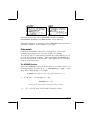
Contents of the calculator’s display
Turn your calculator on once more. At the top of the display you will have
two lines of information that describe the settings of the calculator. The first
line shows the characters:
Page 1-2
RAD XYZ HEX R= 'X'
For details on the meaning of these specifications see Chapter 2 in the
calculator’s user's guide.
The second line shows the characters
{ HOME }
indicating that the HOME directory is the current file directory in the
calculator’s memory.
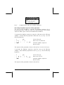
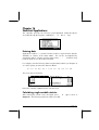
At the bottom of the display you will find a number of labels, namely,
@EDIT @VIEW @@ RCL @@ @@STO@ ! PURGE !CLEAR
associated with the six soft menu keys, F1 through F6:
ABCDEF
The six labels displayed in the lower part of the screen will change depending
on which menu is displayed. But A will always be associated with the first
displayed label, B with the second displayed label, and so on.
Menus
The six labels associated with the keys A through F form part of a menu
of functions. Since the calculator has only six soft menu keys, it only display 6
labels at any point in time. However, a menu can have more than six entries.
Each group of 6 entries is called a Menu page. To move to the next menu
page (if available), press the L (NeXT menu) key. This key is the third key
from the left in the third row of keys in the keyboard.
The TOOL menu
The soft menu keys for the menu currently displayed, known as the TOOL
menu, are associated with operations related to manipulation of variables (see
section on variables in this Chapter):
Page 1-3
@EDIT
A
@VIEW
@@ RCL @@
@@STO@
! PURGE
CLEAR
B
C
D
E
F
EDIT the contents of a variable (see Chapter 2 in this Guide
and Chapter 2 and Appendix L in the user's guide for more
information on editing)
VIEW the contents of a variable
ReCaLl the contents of a variable
STOre the contents of a variable
PURGE a variable
CLEAR the display or stack
These six functions form the first page of the TOOL menu. This menu has
actually eight entries arranged in two pages. The second page is available
by pressing the L (NeXT menu) key. This key is the third key from the left
in the third row of keys in the keyboard.
In this case, only the first two soft menu keys have commands associated with
them. These commands are:
@CASCM
A
@HELP
B
CASCMD: CAS CoMmanD, used to launch a command from
the CAS (Computer Algebraic System) by selecting from a list
HELP facility describing the commands available in the
calculator
Pressing the L key will show the original TOOL menu. Another way to
recover the TOOL menu is to press the I key (third key from the left in the
second row of keys from the top of the keyboard).
Setting time and date
See Chapter 1 in the calculator’s user's guide to learn how to set time and
date.
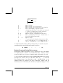
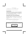
Introducing the calculator’s keyboard
The figure below shows a diagram of the calculator’s keyboard with the
numbering of its rows and columns. Each key has three, four, or five functions.
The main key function correspond to the most prominent label in the key.
Also, the green left-shift key, key (8,1), the red right-shift key, key (9,1), and
Page 1-4
the blue ALPHA key, key (7,1), can be combined with some of the other keys
to activate the alternative functions shown in the keyboard.
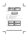
For example, the P key, key(4,4), has the following six functions associated
with it:
P
„´
…N
~p
Main function, to activate the SYMBolic menu
Left-shift function, to activate the MTH (Math) menu
Right-shift function, to activate the CATalog function
ALPHA function, to enter the upper-case letter P
Page 1-5
~„p
~…p
ALPHA-Left-Shift function, to enter the lower-case letter p
ALPHA-Right-Shift function, to enter the symbol π
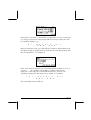
Of the six functions associated with a key only the first four are shown in the
keyboard itself. The figure in next page shows these four labels for the P
key. Notice that the color and the position of the labels in the key, namely,
SYMB, MTH, CAT and P, indicate which is the main function (SYMB), and
which of the other three functions is associated with the left-shift „(MTH),
right-shift … (CAT ), and ~ (P) keys.
For detailed information on the calculator keyboard operation referee to
Appendix B in the calculator’s user's guide.
Selecting calculator modes
This section assumes that you are now at least partially familiar with the use of
choose and dialog boxes (if you are not, please refer to appendix A in the
user's guide).
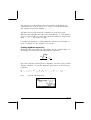
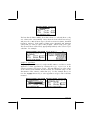
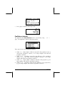
Press the H button (second key from the left on the second row of keys from
the top) to show the following CALCULATOR MODES input form:
Page 1-6
Press the !!@@OK#@ F soft menu key to return to normal display. Examples of
selecting different calculator modes are shown next.
Operating Mode
The calculator offers two operating modes: the Algebraic mode, and the
Reverse Polish Notation (RPN) mode.
The default mode is the Algebraic
mode (as indicated in the figure above), however, users of earlier HP
calculators may be more familiar with the RPN mode.
To select an operating mode, first open the CALCULATOR MODES input form
by pressing the H button. The Operating Mode field will be highlighted.
Select the Algebraic or RPN operating mode by either using the \ key
(second from left in the fifth row from the keyboard bottom), or pressing the
@CHOOSE soft menu key ( B). If using the latter approach, use up and down
arrow keys, — ˜, to select the mode, and press the !!@@OK#@ soft menu key
to complete the operation.
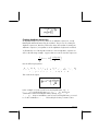
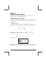
To illustrate the difference between these two operating modes we will
calculate the following expression in both modes:


3.0 ⋅  5.0 −


3.0 ⋅ 3.0 
2.5
+e
23.0
1
3
To enter this expression in the calculator we will first use the equation writer,
‚O. Please identify the following keys in the keyboard, besides the
numeric keypad keys:
!@.#*+-/R
Q¸Ü‚Oš™˜—`
The equation writer is a display mode in which you can build mathematical
expressions using explicit mathematical notation including fractions,
derivatives, integrals, roots, etc. To use the equation writer for writing the
expression shown above, use the following keystrokes:
‚OR3.*!Ü5.-
Page 1-7
1./3.*3.
—————
/23.Q3™™™+!¸2.5`
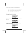
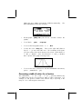
After pressing `the calculator displays the expression:
√ (3.*(5.-1/(3.*3.))/23.^3+EXP(2.5))
Pressing `again will provide the following value (accept Approx mode on,
if asked, by pressing !!@@OK#@):
You could also type the expression directly into the display without using the
equation writer, as follows:
R!Ü3.*!Ü5.1/3.*3.™
/23.Q3+!¸2.5`
to obtain the same result.
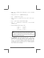
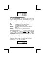
Change the operating mode to RPN by first pressing the H button. Select
the RPN operating mode by either using the \key, or pressing the @CHOOSE
soft menu key. Press the !!@@OK#@ F soft menu key to complete the operation.
The display, for the RPN mode looks as follows:
Notice that the display shows several levels of output labeled, from bottom to
top, as 1, 2, 3, etc. This is referred to as the stack of the calculator. The
Page 1-8
different levels are referred to as the stack levels, i.e., stack level 1, stack level
2, etc.
Basically, what RPN means is that, instead of writing an operation such as 3
+ 2, in the calculator by using
3+2`
we write first the operands, in the proper order, and then the operator, i.e.,
3`2`+
As you enter the operands, they occupy different stack levels. Entering
3`puts the number 3 in stack level 1. Next, entering 2`pushes
the 3 upwards to occupy stack level 2. Finally, by pressing +, we are
telling the calculator to apply the operator, or program, + to the objects
occupying levels 1 and 2. The result, 5, is then placed in level 1.
Let's try some other simple operations before trying the more complicated
expression used earlier for the algebraic operating mode:
123/32
2
4
3
√27
123`32/
4`2Q
27`R3@»
Notice the position of the y and the x in the last two operations. The base in
the exponential operation is y (stack level 2) while the exponent is x (stack
level 1) before the key Q is pressed. Similarly, in the cubic root operation,
y (stack level 2) is the quantity under the root sign, and x (stack level 1) is the
root.
Try the following exercise involving 3 factors: (5 + 3) × 2
5`3`+
2X
Calculates (5 +3) first.
Completes the calculation.
Let's try now the expression proposed earlier:
Page 1-9


3 ⋅ 5 −
23
3`
5`
3`
3*
Y
*
23`
3Q
/
2.5
!¸
+
R


3⋅3
2.5
+e
1
3
Enter 3 in level 1
Enter 5 in level 1, 3 moves to level 2
Enter 3 in level 1, 5 moves to level 2, 3 to level 3
Place 3 and multiply, 9 appears in level 1
1/(3×3), last value in lev. 1; 5 in level 2; 3 in level 3
5 - 1/(3×3) , occupies level 1 now; 3 in level 2
3× (5 - 1/(3×3)), occupies level 1 now.
Enter 23 in level 1, 14.66666 moves to level 2.
3
Enter 3, calculate 23 into level 1. 14.666 in lev. 2.
3
(3× (5-1/(3×3)))/23 into level 1
Enter 2.5 level 1
2.5
e , goes into level 1, level 2 shows previous value.
3
2.5
(3× (5 - 1/(3×3)))/23 + e = 12.18369, into lev. 1.
3
2.5
√((3× (5 - 1/(3×3)))/23 + e ) = 3.4905156, into 1.
To select between the ALG vs. RPN operating mode, you can also set/clear
system flag 95 through the following keystroke sequence:
H @)FLAGS —„—„—„ — @@CHK@
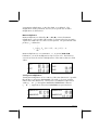
Number Format and decimal dot or comma
Changing the number format allows you to customize the way real numbers
are displayed by the calculator. You will find this feature extremely useful in
operations with powers of tens or to limit the number of decimals in a result.
To select a number format, first open the CALCULATOR MODES input form by
pressing the H button. Then, use the down arrow key, ˜, to select the
option Number format. The default value is Std, or Standard format. In the
standard format, the calculator will show floating-point numbers with the
maximum precision allowed by the calculator (12 significant digits). To learn
Page 1-10
more about reals, see Chapter 2 in this Guide. To illustrate this and other
number formats try the following exercises:
•
Standard format:
This mode is the most used mode as it shows numbers in the most familiar
notation. Press the !!@@OK#@ soft menu key, with the Number format set to Std,
to return to the calculator display.
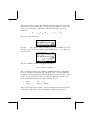
Enter the number
123.4567890123456 (with16 significant figures). Press the ` key.
The number is rounded to the maximum 12 significant figures, and is
displayed as follows:
•
Fixed format with decimals:
Press the H button. Next, use the down arrow key, ˜, to select the
option Number format. Press the @CHOOSE soft menu key ( B), and select
the option Fixed with the arrow down key ˜.
Press the right arrow key, ™, to highlight the zero in front of the option
Fix. Press the @CHOOSE soft menu key and, using the up and down arrow
keys, —˜, select, say, 3 decimals.
Press the !!@@OK#@ soft menu key to complete the selection:
Page 1-11
Press the !!@@OK#@ soft menu key return to the calculator display.
number now is shown as:
The
Notice how the number is rounded, not truncated. Thus, the number
123.4567890123456, for this setting, is displayed as 123.457, and not
as 123.456 because the digit after 6 is > 5):
•
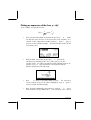
Scientific format
To set this format, start by pressing the H button. Next, use the down
arrow key, ˜, to select the option Number format. Press the @CHOOSE soft
menu key ( B), and select the option Scientific with the arrow down key
˜.
Keep the number 3 in front of the Sci. (This number can be
changed in the same fashion that we changed the Fixed number of
decimals in the example above).
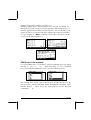
Press the !!@@OK#@ soft menu key return to the calculator display.
number now is shown as:
The
Page 1-12
This result, 1.23E2, is the calculator’s version of powers-of-ten notation,
2
i.e., 1.235 × 10 . In this, so-called, scientific notation, the number 3 in
front of the Sci number format (shown earlier) represents the number of
significant figures after the decimal point. Scientific notation always
includes one integer figure as shown above. For this case, therefore, the
number of significant figures is four.
•
Engineering format
The engineering format is very similar to the scientific format, except that
the powers of ten are multiples of three. To set this format, start by
pressing the H button. Next, use the down arrow key, ˜, to select
the option Number format. Press the @CHOOSE soft menu key ( B), and
select the option Engineering with the arrow down key ˜.
Keep the
number 3 in front of the Eng. (This number can be changed in the same
fashion that we changed the Fixed number of decimals in an earlier
example).
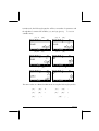
Press the ! @@OK#@ soft menu key return to the calculator display.
number now is shown as:
The
Because this number has three figures in the integer part, it is shown with
four significative figures and a zero power of ten, while using the
Engineering format. For example, the number 0.00256, will be shown as:
Page 1-13
•
Decimal comma vs. decimal point
Decimal points in floating-point numbers can be replaced by commas, if
the user is more familiar with such notation. To replace decimal points for
commas, change the FM option in the CALCULATOR MODES input form
to commas, as follows (Notice that we have changed the Number Format
to Std):
•
Press the H button. Next, use the down arrow key, ˜, once, and the
right arrow key, ™, twice, to highlight the option __FM,.
To select
commas, press the @CHECK soft menu key (i.e., the B key). The input form
will look as follows:
•
Press the ! @@OK#@ soft menu key return to the calculator display.
number 123.456789012, entered earlier, now is shown as:
The
Angle Measure
Trigonometric functions, for example, require arguments representing plane
angles. The calculator provides three different Angle Measure modes for
working with angles, namely:
•
•
o
Degrees: There are 360 degrees (360 ) in a complete circumference.
r
Radians: There are 2π radians (2π ) in a complete circumference.
Page 1-14
•
g
Grades: There are 400 grades (400 ) in a complete circumference.
The angle measure affects the trig functions like SIN, COS, TAN and
associated functions.
To change the angle measure mode, use the following procedure:
•
Press the H button. Next, use the down arrow key, ˜, twice. Select
the Angle Measure mode by either using the \key (second from left in
the fifth row from the keyboard bottom), or pressing the @CHOOSE soft menu
key ( B).
If using the latter approach, use up and down arrow
keys,— ˜, to select the preferred mode, and press the !!@@OK#@ F soft
menu key to complete the operation.
For example, in the following
screen, the Radians mode is selected:
Coordinate System
The coordinate system selection affects the way vectors and complex numbers
are displayed and entered. To learn more about complex numbers and
vectors, see Chapters 4 and 8, respectively, in this Guide. There are three
coordinate systems available in the calculator: Rectangular (RECT), Cylindrical
(CYLIN), and Spherical (SPHERE). To change coordinate system:
•
Press the H button. Next, use the down arrow key, ˜, three times.
Select the Coord System mode by either using the \ key (second from
left in the fifth row from the keyboard bottom), or pressing the @CHOOSE soft
menu key ( B). If using the latter approach, use up and down arrow
keys,— ˜, to select the preferred mode, and press the !!@@OK#@ F soft
menu key to complete the operation.
For example, in the following
screen, the Polar coordinate mode is selected:
Page 1-15
Selecting CAS settings
CAS stands for Computer Algebraic System. This is the mathematical core of
the calculator where the symbolic mathematical operations and functions are
programmed. The CAS offers a number of settings can be adjusted according
to the type of operation of interest. To see the optional CAS settings use the
following:
•
Press the H button to activate the CALCULATOR MODES input form.
•
To change CAS settings press the @@ CAS@@ soft menu key. The default values
of the CAS setting are shown below:
•
To navigate through the many options in the CAS MODES input form, use
the arrow keys: š™˜—.
•
To select or deselect any of the settings shown above, select the underline
before the option of interest, and toggle the @@CHK@@ soft menu key until the
right setting is achieved. When an option is selected, a check mark will
be shown in the underline (e.g., the Rigorous and Simp Non-Rational
Page 1-16
options above).
Unselected options will show no check mark in the
underline preceding the option of interest (e.g., the _Numeric, _Approx,
_Complex, _Verbose, _Step/Step, _Incr Pow options above).
•
After having selected and unselected all the options that you want in the
CAS MODES input form, press the @@@OK@@@ soft menu key. This will take you
back to the CALCULATOR MODES input form.
To return to normal
calculator display at this point, press the @@@OK@@@ soft menu key once more.
Explanation of CAS settings
•
•
•
•
•
•
•
•
•
•
Indep var: The independent variable for CAS applications. Typically, VX
= ‘X’.
Modulo: For operations in modular arithmetic this variable holds the
modulus or modulo of the arithmetic ring (see Chapter 5 in the calculator’s
user's guide).
Numeric: If set, the calculator produces a numeric, or floating-point result,
in calculations.
Approx: If set, Approximate mode uses numerical results in calculations. If
unchecked, the CAS is in Exact mode, which produces symbolic results in
algebraic calculations.
Complex: If set, complex number operations are active. If unchecked the
CAS is in Real mode, i.e., real number calculations are the default. See
Chapter 4 for operations with complex numbers.
Verbose: If set, provides detailed information in certain CAS operations.
Step/Step: If set, provides step-by-step results for certain CAS operations.
Useful to see intermediate steps in summations, derivatives, integrals,
polynomial operations (e.g., synthetic division), and matrix operations.
Incr Pow: Increasing Power, means that, if set, polynomial terms are
shown in increasing order of the powers of the independent variable.
Rigorous: If set, calculator does not simplify the absolute value function
|X| to X.
Simp Non-Rational: If set, the calculator will try to simplify non-rational
expressions as much as possible.
Selecting Display modes
Page 1-17
The calculator display can be customized to your preference by selecting
different display modes. To see the optional display settings use the following:
•
First, press the H button to activate the CALCULATOR MODES input
form. Within the CALCULATOR MODES input form, press the @@DISP@ soft
menu key (D) to display the DISPLAY MODES input form.
•
To navigate through the many options in the DISPLAY MODES input form,
use the arrow keys: š™˜—.
•
To select or deselect any of the settings shown above, that require a check
mark, select the underline before the option of interest, and toggle the
@@CHK@@ soft menu key until the right setting is achieved. When an option is
selected, a check mark will be shown in the underline (e.g., the Textbook
option in the Stack: line above). Unselected options will show no check
mark in the underline preceding the option of interest (e.g., the _Small,
_Full page, and _Indent options in the Edit: line above).
•
To select the Font for the display, highlight the field in front of the Font:
option in the DISPLAY MODES input form, and use the @CHOOSE soft menu
key (B).
•
After having selected and unselected all the options that you want in the
DISPLAY MODES input form, press the @@@OK@@@ soft menu key. This will take
you back to the CALCULATOR MODES input form. To return to normal
calculator display at this point, press the @@@OK@@@ soft menu key once more.
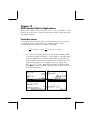
Selecting the display font
First, press the H button to activate the CALCULATOR MODES input form.
Within the CALCULATOR MODES input form, press the @@DISP@ soft menu key
Page 1-18
(D) to display the DISPLAY MODES input form. The Font: field is
highlighted, and the option Ft8_0:system 8 is selected. This is the default
value of the display font. Pressing the @CHOOSE soft menu key (B), will
provide a list of available system fonts, as shown below:
The options available are three standard System Fonts (sizes 8, 7, and 6) and
a Browse.. option. The latter will let you browse the calculator memory for
additional fonts that you may have created or downloaded into the calculator.
Practice changing the display fonts to sizes 7 and 6. Press the OK soft menu
key to effect the selection. When done with a font selection, press the @@@OK@@@
soft menu key to go back to the CALCULATOR MODES input form. To return
to normal calculator display at this point, press the @@@OK@@@ soft menu key once
more and see how the stack display change to accommodate the different font.
Selecting properties of the line editor
First, press the H button to activate the CALCULATOR MODES input form.
Within the CALCULATOR MODES input form, press the @@DISP@ soft menu key
(D) to display the DISPLAY MODES input form. Press the down arrow key,
˜, once, to get to the Edit line. This line shows three properties that can be
modified. When these properties are selected (checked) the following effects
are activated:
_Small
_Full page
_Indent
Changes font size to small
Allows to place the cursor after the end of the line
Auto indent cursor when entering a carriage return
Instructions on the use of the line editor are presented in Chapter 2 in this
guide.
Page 1-19
Selecting properties of the Stack
First, press the H button to activate the CALCULATOR MODES input form.
Within the CALCULATOR MODES input form, press the @@DISP@ soft menu key
(D) to display the DISPLAY MODES input form. Press the down arrow key,
˜, twice, to get to the Stack line. This line shows two properties that can be
modified. When these properties are selected (checked) the following effects
are activated:
_Small
Changes font size to small. This maximizes the amount of
information displayed on the screen. Note, this selection
overrides the font selection for the stack display.
_Textbook
Displays mathematical expressions in graphical mathematical
notation
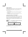
To illustrate these settings, either in algebraic or RPN mode, use the equation
writer to type the following definite integral:
‚O…Á0™„虄¸\x™x`
In Algebraic mode, the following screen shows the result of these keystrokes
with neither _Small nor _Textbook are selected:
With the _Small option selected only, the display looks as shown below:
With the _Textbook option selected (default value), regardless of whether the
_Small option is selected or not, the display shows the following result:
Page 1-20
Selecting properties of the equation writer (EQW)
First, press the H button to activate the CALCULATOR MODES input form.
Within the CALCULATOR MODES input form, press the @@DISP@ soft menu key
(D) to display the DISPLAY MODES input form. Press the down arrow key,
˜, three times, to get to the EQW (Equation Writer) line. This line shows
two properties that can be modified. When these properties are selected
(checked) the following effects are activated:
_Small
_Small Stack Disp
Changes font size to small while using the equation
editor
Shows small font in the stack after using the equation
editor
Detailed instructions on the use of the equation editor (EQW) are presented
elsewhere in this manual.
For the example of the integral
∫
∞
0
e − X dX , presented above, selecting the
_Small Stack Disp in the EQW line of the DISPLAY MODES input form
produces the following display:
References
Additional references on the subjects covered in this Chapter can be found in
Chapter 1 and Appendix C of the calculator’s user's guide.
Page 1-21
Page 1-22
Chapter 2
Introducing the calculator
In this chapter we present a number of basic operations of the calculator
including the use of the Equation Writer and the manipulation of data objects
in the calculator. Study the examples in this chapter to get a good grasp of
the capabilities of the calculator for future applications.
Calculator objects
Some of the most commonly used objects are: reals (real numbers, written with
a decimal point, e.g., -0.0023, 3.56), integers (integer numbers, written
without a decimal point, e.g., 1232, -123212123), complex numbers (written
as an ordered pair, e.g., (3,-2)), lists, etc. Calculator objects are described in
Chapters 2 and 24 in the calculator’s user guide.
Editing expressions in the stack
In this section we present examples of expression editing directly into the
calculator display or stack.
Creating arithmetic expressions
For this example, we select the Algebraic operating mode and select a Fix
format with 3 decimals for the display. We are going to enter the arithmetic
expression:
1.0
7.5
5.0 ⋅
3.0 − 2.0 3
1.0 +
To enter this expression use the following keystrokes:
5.*„Ü1.+1./7.5™/
„ÜR3.-2.Q3
The resulting expression is: 5*(1+1/7.5)/( 3-2^3).
Press ` to get the expression in the display as follows:
Page 2-1
Notice that, if your CAS is set to EXACT (see Appendix C in user's guide) and
you enter your expression using integer numbers for integer values, the result
is a symbolic quantity, e.g.,
5*„Ü1+1/7.5™/
„ÜR3-2Q3
Before producing a result, you will be asked to change to Approximate mode.
Accept the change to get the following result (shown in Fix decimal mode with
three decimal places – see Chapter 1):
In this case, when the expression is entered directly into the stack, as soon as
you press `, the calculator will attempt to calculate a value for the
expression. If the expression is entered between quotes, however, the
calculator will reproduce the expression as entered. For example:
³5*„Ü1+1/7.5™/
„ÜR3-2Q3`
The result will be shown as follows:
Page 2-2
To evaluate the expression we can use the EVAL function, as follows:
µ„î
If the CAS is set to Exact, you will be asked to approve changing the CAS
setting to Approx. Once this is done, you will get the same result as before.
An alternative way to evaluate the expression entered earlier between quotes
is by using the option …ï.
We will now enter the expression used above when the calculator is set to the
RPN operating mode. We also set the CAS to Exact and the display to
Textbook. The keystrokes to enter the expression between quotes are the
same used earlier, i.e.,
…³5*„Ü1+1/7.5™/
„ÜR3-2Q3`
Resulting in the output
Press ` once more to keep two copies of the expression available in the
stack for evaluation. We first evaluate the expression using the function EVAL,
and next using the function ÆNUM: µ .
Page 2-3
This expression is semi-symbolic in the sense that there are floating-point
components to the result, as well as a √3. Next, we switch stack locations
and evaluate using function ÆNUM: ™…ï.
This latter result is purely numerical, so that the two results in the stack,
although representing the same expression, seem different. To verify that they
are not, we subtract the two values and evaluate this difference using function
EVAL: -µ. The result is zero (0.).
For additional information on editing arithmetic expressions in the display or
stack, see Chapter 2 in the calculator’s user's guide.
Creating algebraic expressions
Algebraic expressions include not only numbers, but also variable names. As
an example, we will enter the following algebraic expression:
x
R +2L
R+ y
b
2L 1 +
We set the calculator operating mode to Algebraic, the CAS to Exact, and the
display to Textbook. To enter this algebraic expression we use the following
keystrokes:
2*~l*R„Ü1+~„x/~r™/„
Ü ~r+~„y™+2*~l/~„b
Press ` to get the following result:
Page 2-4
Entering this expression when the calculator is set in the RPN mode is exactly
the same as this Algebraic mode exercise.
For additional information on editing algebraic expressions in the calculator’s
display or stack see Chapter 2 in the calculator’s user's guide.
Using the Equation Writer (EQW) to create expressions
The equation writer is an extremely powerful tool that not only let you enter or
see an equation, but also allows you to modify and work/apply functions on
all or part of the equation.
The Equation Writer is launched by pressing the keystroke combination
‚O (the third key in the fourth row from the top in the keyboard). The
resulting screen is the following. Press L to see the second menu page:
The six soft menu keys for the Equation Writer activate functions EDIT, CURS,
BIG, EVAL, FACTOR, SIMPLIFY, CMDS, and HELP. Detailed information on
these functions is provided in Chapter 3 of the calculator’s user's guide.
Creating arithmetic expressions
Entering arithmetic expressions in the Equation Writer is very similar to
entering an arithmetic expression in the stack enclosed in quotes. The main
difference is that in the Equation Writer the expressions produced are written
in “textbook” style instead of a line-entry style. For example, try the following
keystrokes in the Equation Writer screen: 5/5+2
The result is the expression
Page 2-5
The cursor is shown as a left-facing key. The cursor indicates the current
edition location. For example, for the cursor in the location indicated above,
type now:
*„Ü5+1/3
The edited expression looks as follows:
Suppose that you want to replace the quantity between parentheses in the
2
denominator (i.e., 5+1/3) with (5+π /2). First, we use the delete key (ƒ)
2
delete the current 1/3 expression, and then we replace that fraction with π /2,
as follows:
ƒƒƒ„ìQ2
When hit this point the screen looks as follows:
In order to insert the denominator 2 in the expression, we need to highlight
2
the entire π expression. We do this by pressing the right arrow key (™)
once. At that point, we enter the following keystrokes:
/2
Page 2-6
The expression now looks as follows:
Suppose that now you want to add the fraction 1/3 to this entire expression,
i.e., you want to enter the expression:
5
5 + 2 ⋅ (5 +
π
+
2
2
)
1
3
First, we need to highlight the entire first term by using either the right arrow
(™) or the upper arrow (—) keys, repeatedly, until the entire expression is
highlighted, i.e., seven times, producing:
NOTE: Alternatively, from the original position of the cursor (to the right of the
2
2 in the denominator of π /2), we can use the keystroke combination ‚—
, interpreted as (‚ ‘ ).
Once the expression is highlighted as shown above, type +1/3 to
add the fraction 1/3. Resulting in:
Page 2-7
Creating algebraic expressions
An algebraic expression is very similar to an arithmetic expression, except
that English and Greek letters may be included. The process of creating an
algebraic expression, therefore, follows the same idea as that of creating an
arithmetic expression, except that use of the alphabetic keyboard is included.
To illustrate the use of the Equation Writer to enter an algebraic equation we
will use the following example. Suppose that we want to enter the expression:
2
3
 x + 2 µ ⋅ ∆y 

1/ 3
 θ

λ + e − µ ⋅ LN 
Use the following keystrokes:
2 / R3 ™™ * ~‚n + „¸\ ~‚m
™™ * ‚¹ ~„x + 2 * ~‚m * ~‚c
~„y ——— / ~‚t Q1/3
This results in the output:
In this example we used several lower-case English letters, e.g., x
(~„x), several Greek letters, e.g., λ (~‚n), and even a
combination of Greek and English letters, namely, ∆y (~‚c
~„y). Keep in mind that to enter a lower-case English letter, you need
to use the combination: ~„ followed by the letter you want to enter.
Page 2-8
Also, you can always copy special characters by using the CHARS menu
(…±) if you don’t want to memorize the keystroke combination that
produces it. A listing of commonly used ~‚keystroke combinations
was listed in an earlier section.
For additional information on editing, evaluating, factoring, and simplifying
algebraic expressions see Chapter 2 of the calculator’s user's guide.
Organizing data in the calculator
You can organize data in your calculator by storing variables in a directory
tree. The basis of the calculator’s directory tree is the HOME directory
described next.
The HOME directory
To get to the HOME directory, press the UPDIR function („§) -- repeat as
needed -- until the {HOME} spec is shown in the second line of the display
header. Alternatively, use „ (hold) §. For this example, the HOME
directory contains nothing but the CASDIR. Pressing J will show the
variables in the soft menu keys:
Subdirectories
To store your data in a well organized directory tree you may want to create
subdirectories under the HOME directory, and more subdirectories within
subdirectories, in a hierarchy of directories similar to folders in modern
computers. The subdirectories will be given names that may reflect the
contents of each subdirectory, or any arbitrary name that you can think off.
For details on manipulation of directories see Chapter 2 in the calculator’s
user's guide.
Page 2-9
Variables
Variables are similar to files on a computer hard drive. One variable can
store one object (numerical values, algebraic expressions, lists, vectors,
matrices, programs, etc). Variables are referred to by their names, which can
be any combination of alphabetic and numerical characters, starting with a
letter (either English or Greek). Some non-alphabetic characters, such as the
arrow (→) can be used in a variable name, if combined with an alphabetical
character. Thus, ‘→A’ is a valid variable name, but ‘→’ is not. Valid
examples of variable names are: ‘A’, ‘B’, ‘a’, ‘b’, ‘α’, ‘β’, ‘A1’, ‘AB12’,
‘ÆA12’,’Vel’,’Z0’,’z1’, etc.
A variable can not have the same name as a function of the calculator. The
reserved calculator variable names are the following: ALRMDAT, CST, EQ,
EXPR, IERR, IOPAR, MAXR, MINR, PICT, PPAR, PRTPAR, VPAR, ZPAR, der_, e,
i, n1,n2, …, s1, s2, …, ΣDAT, ΣPAR, π, ∞
Variables can be organized into sub-directories (see Chapter 2 in the
calculator’s user's guide).
Typing variable names
To name variables, you will have to type strings of letters at once, which may
or may not be combined with numbers. To type strings of characters you can
lock the alphabetic keyboard as follows:
~~ locks the alphabetic keyboard in upper case. When locked in this
fashion, pressing the „ before a letter key produces a lower case letter,
while pressing the ‚ key before a letter key produces a special character.
If the alphabetic keyboard is already locked in upper case, to lock it in lower
case, type, „~
~~„~ locks the alphabetic keyboard in lower case. When locked
in this fashion, pressing the „ before a letter key produces an upper case
letter. To unlock lower case, press „~
Page 2-10
To unlock the upper-case locked keyboard, press ~
Try the following exercises:
³~~math1~`
³~~m„a„t„h~`
³~~m„~at„h~`
The calculator display will show the following (left-hand side is Algebraic
mode, right-hand side is RPN mode):
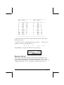
Creating variables
The simplest way to create a variable is by using the K . The following
examples are used to store the variables listed in the following table (Press
J if needed to see variables menu):
•
Name
Contents
Type
α
A12
Q
R
z1
p1
-0.25
5
3×10
‘r/(m+r)'
[3,2,1]
3+5i
<< → r 'π*r^2' >>
real
real
algebraic
vector
complex
program
Algebraic mode
To store the value of –0.25 into variable α: 0.25\
K ~‚a. AT this point, the screen will look as follows:
Page 2-11
Press ` to create the variable. The variable is now shown in the
soft menu key labels:
The following are the keystrokes required to enter the remaining
variables:
A12: 3V5K~a12`
Q: ³~„r/„Ü
~„m+~„r™™ K~q`
R: „Ô3‚í2‚í1™ K~r`
z1: 3+5*„¥ K~„z1` (Accept
change to Complex mode if asked).
p1: ‚å‚é~„r³„ì*
~„rQ2™™™ K~„p1`..
The screen, at this point, will look as follows:
You will see six of the seven variables listed at the bottom of the
screen: p1, z1, R, Q, A12, α.
Page 2-12
•
RPN mode
(Use I\@@OK@@ to change to RPN mode). Use the following
keystrokes to store the value of –0.25 into variable α:
0.25\` ~‚a`. At this point, the screen
will look as follows:
This expression means that the value –0.25 is ready to be stored into
α. Press K to create the variable. The variable is now shown in
the soft menu key labels:
5
To enter the value 3×10 into A12, we can use a shorter version of
the procedure: 3V5³~a12` K
Here is a way to enter the contents of Q:
Q: ³~„r/„Ü
~„m+~„r™™ ³~q` K
To enter the value of R, we can use an even shorter version of the
procedure:
R: „Ô3#2#1™ ³K
Notice that to separate the elements of a vector in RPN mode we can
use the space key (#), rather than the comma (‚í ) used
above in Algebraic mode.
z1: ³3+5*„¥ ³~„z1 K
Page 2-13
p1: ‚å‚é~„r³„ì*
~„rQ2™™™ ³ ~„p1™` K.
The screen, at this point, will look as follows:
You will see six of the seven variables listed at the bottom of the
screen: p1, z1, R, Q, A12, α.
Checking variables contents
The simplest way to check a variable content is by pressing the soft menu key
label for the variable. For example, for the variables listed above, press the
following keys to see the contents of the variables:
Algebraic mode
Type these keystrokes: J@@ @@ ` @@@R@@ `@@@ @@@ `. At this point, the
screen looks as follows:
RPN mode
In RPN mode, you only need to press the corresponding soft menu key label to
get the contents of a numerical or algebraic variable. For the case under
consideration, we can try peeking into the variables z1, R, Q, A12, α, and A,
created above, as follows: J@@ @@ @@@R@@ @@@ @@ @@A @@ @@ @@
At this point, the screen looks like this:
Page 2-14
Using the right-shift key ‚ followed by soft menu key labels
This approach for viewing the contents of a variable works the same in both
Algebraic and RPN modes. Try the following examples in either mode:
J‚@@ @@ ‚ @@ @@ ‚ @@@R@@ ‚@@@ @@ ‚ @@A @@
This produces the following screen (Algebraic mode in the left, RPN in the
right)
Notice that this time the contents of program p1 are listed in the screen. To
see the remaining variables in this directory, use:
@@@ @@
Listing the contents of all variables in the screen
Use the keystroke combination ‚˜ to list the contents of all variables in
the screen. For example:
Press $ to return to normal calculator display.
Page 2-15
Deleting variables
The simplest way of deleting variables is by using function PURGE. This
function can be accessed directly by using the TOOLS menu (I), or by
using the FILES menu „¡@@OK@@ .
Using function PURGE in the stack in Algebraic mode
Our variable list contains variables p1, z1, Q, R, and α. We will use
command PURGE to delete variable p1. Press I @PURGE@ J@@ @@ `.
The screen will now show variable p1 removed:
You can use the PURGE command to erase more than one variable by placing
their names in a list in the argument of PURGE. For example, if now we
wanted to purge variables R and Q, simultaneously, we can try the following
exercise. Press :
I @PURGE@ „ä³ J@@@R!@@ ™ ‚í ³ J@@@ !@@
At this point, the screen will show the following command ready to be
executed:
To finish deleting the variables, press `. The screen will now show the
remaining variables:
Using function PURGE in the stack in RPN mode
Assuming that our variable list contains the variables p1, z1, Q, R, and α.
We will use command PURGE to delete variable p1. Press ³@@ @@ `
I @PURGE@. The screen will now show variable p1 removed:
Page 2-16
To delete two variables simultaneously, say variables R and Q, first create a
list (in RPN mode, the elements of the list need not be separated by commas
as in Algebraic mode):
J „ä³ @@@R!@@ ™ ³ @@@ !@@ `
Then, press I@PURGE@ use to purge the variables.
Additional information on variable manipulation is available in Chapter 2 of
the calculator’s user's guide.
UNDO and CMD functions
Functions UNDO and CMD are useful for recovering recent commands, or to
revert an operation if a mistake was made. These functions are associated
with the HIST key: UNDO results from the keystroke sequence ‚¯, while
CMD results from the keystroke sequence „®.
CHOOSE boxes vs. Soft MENU
In some of the exercises presented in this chapter we have seen menu lists of
commands displayed in the screen. This menu lists are referred to as
CHOOSE boxes. Herein we indicate the way to change from CHOSE boxes
to Soft MENUs, and vice versa, through an exercise.
Although not applied to a specific example, the present exercise shows the
two options for menus in the calculator (CHOOSE boxes and soft MENUs). In
this exercise, we use the ORDER command to reorder variables in a directory,
we use:
„°˜
Show PROG menu list and select MEMORY
Page 2-17
@@OK@@ ˜˜˜˜
Show the MEMORY menu list and select DIRECTORY
@@OK@@ ——
Show the DIRECTORY menu list and select ORDER
@@OK@@
activate the ORDER command
There is an alternative way to access these menus as soft MENU keys, by
setting system flag 117. (For information on Flags see Chapters 2 and 24 in
the calculator’s user's guide). To set this flag try the following:
H @FLAGS! ———————
The screen shows flag 117 not set (CHOOSE boxes), as shown here:
Page 2-18
Press the @CHECK! soft menu key to set flag 117 to soft MENU. The screen will
reflect that change:
Press twice to return to normal calculator display.
Now, we’ll try to find the ORDER command using similar keystrokes to those
used above, i.e., we start with „°. Notice that instead of a menu list,
we get soft menu labels with the different options in the PROG menu, i.e.,
Press B to select the MEMORY soft menu ()@@MEM@@). The display now shows:
Press E to select the DIRECTORY soft menu ()@@DIR@@)
The ORDER command is not shown in this screen. To find it we use the L
key to find it:
Page 2-19
To activate the ORDER command we press the C(@ORDER) soft menu key.
References
For additional information on entering and manipulating expressions in the
display or in the Equation Writer see Chapter 2 of the calculator’s user's
guide. For CAS (Computer Algebraic System) settings, see Appendix C in the
calculator’s user’s guide. For information on Flags see, Chapter 24 in the
calculator’s user’s guide.
Page 2-20
Chapter 3
Calculations with real numbers
This chapter demonstrates the use of the calculator for operations and
functions related to real numbers. The user should be acquainted with the
keyboard to identify certain functions available in the keyboard (e.g., SIN,
COS, TAN, etc.). Also, it is assumed that the reader knows how to change
the calculator’s operating system (Chapter 1), use menus and choose boxes
(Chapter 1), and operate with variables (Chapter 2).
Examples of real number calculations
To perform real number calculations it is preferred to have the CAS set to Real
(as opposed to Complex) mode. Exact mode is the default mode for most
operations. Therefore, you may want to start your calculations in this mode.
Some operations with real numbers are illustrated next:
•
Use the \ key for changing sign of a number.
For example, in ALG mode, \2.5`.
In RPN mode, e.g., 2.5\.
•
Use the Ykey to calculate the inverse of a number.
For example, in ALG mode, Y2`.
In RPN mode use 4`Y.
•
For addition, subtraction, multiplication, division, use the proper
operation key, namely, + - * /.
Examples in ALG mode:
3.7
6.3
4.2
2.3
+
*
/
5.2
8.5
2.5
4.5
`
`
`
`
Examples in RPN mode:
3.7` 5.2 +
Page 3-1
6.3` 8.5 4.2` 2.5 *
2.3` 4.5 /
Alternatively, in RPN mode, you can separate the operands with a
space (#) before pressing the operator key. Examples:
3.7#5.2
6.3#8.5
4.2#2.5
2.3#4.5
•
+
*
/
Parentheses („Ü) can be used to group operations, as well as to
enclose arguments of functions.
In ALG mode:
„Ü5+3.2™/„Ü72.2`
In RPN mode, you do not need the parenthesis, calculation is done
directly on the stack:
5`3.2`+7`2.2`-/
In RPN mode, typing the expression between quotes will allow you to
enter the expression like in algebraic mode:
³„Ü5+3.2/
„Ü72.2`µ
For both, ALG and RPN modes, using the Equation Writer:
‚O5+3.2™/7-2.2
The expression can be evaluated within the Equation writer, by using
————@EVAL@ or, ‚—@EVAL@
•
The absolute value function, ABS, is available through „Ê.
Example in ALG mode:
Page 3-2
„Ê \2.32`
Example in RPN mode:
2.32\„Ê
•
The square function, SQ, is available through „º.
Example in ALG mode:
„º\2.3`
Example in RPN mode:
2.3\„º
The square root function, √, is available through the R key. When
calculating in the stack in ALG mode, enter the function before the
argument, e.g.,
R123.4`
In RPN mode, enter the number first, then the function, e.g.,
123.4R
•
The power function, ^, is available through the Q key. When
calculating in the stack in ALG mode, enter the base (y) followed by
the Q key, and then the exponent (x), e.g.,
5.2Q1.25
In RPN mode, enter the number first, then the function, e.g.,
5.2`1.25Q
•
The root function, XROOT(y,x), is available through the keystroke
combination ‚». When calculating in the stack in ALG mode,
Page 3-3
enter the function XROOT followed by the arguments (y,x), separated
by commas, e.g.,
‚»3‚í 27`
In RPN mode, enter the argument y, first, then, x, and finally the
function call, e.g.,
27`3‚»
•
Logarithms of base 10 are calculated by the keystroke combination
‚Ã (function LOG) while its inverse function (ALOG, or
antilogarithm) is calculated by using „Â. In ALG mode, the
function is entered before the argument:
‚Ã2.45`
„Â\2.3`
In RPN mode, the argument is entered before the function
2.45 ‚Ã
2.3\ „Â
Using powers of 10 in entering data
-2
Powers of ten, i.e., numbers of the form -4.5×10 , etc., are entered by using
the V key. For example, in ALG mode:
\4.5V\2`
Or, in RPN mode:
4.5\V2\`
•
Natural logarithms are calculated by using ‚¹ (function LN)
while the exponential function (EXP) is calculated by using „¸.
In ALG mode, the function is entered before the argument:
‚¹2.45`
„¸\2.3`
In RPN mode, the argument is entered before the function
Page 3-4
2.45` ‚¹
2.3\` „¸
•
Three trigonometric functions are readily available in the keyboard:
sine (S), cosine (T), and tangent (U). Arguments of these
functions are angles in either degrees, radians, grades. The
following examples use angles in degrees (DEG):
In ALG mode:
S30`
T45`
U135`
In RPN mode:
30S
45T
135U
•
The inverse trigonometric functions available in the keyboard are the
arcsine („¼), arccosine („¾), and arctangent („À).
The answer from these functions will be given in the selected angular
measure (DEG, RAD, GRD). Some examples are shown next:
In ALG mode:
„¼0.25`
„¾0.85`
„À1.35`
In RPN mode:
0.25„¼
0.85„¾
1.35„À
All the functions described above, namely, ABS, ABS, SQ, √, ^, XROOT,
LOG, ALOG, LN, EXP, SIN, COS, TAN, ASIN, ACOS, ATAN, can be
combined with the fundamental operations (+-*/) to form more
complex expressions. The Equation Writer, whose operations is described in
Chapter 2, is ideal for building such expressions, regardless of the calculator
operation mode.
Page 3-5
Real number functions in the MTH menu
The MTH („´) menu include a number of mathematical functions mostly
applicable to real numbers. With the default setting of CHOOSE boxes for
system flag 117 (see Chapter 2), the MTH menu shows the following functions:
The functions are grouped by the type of argument (1. vectors, 2. matrices, 3.
lists, 7. probability, 9. complex) or by the type of function (4. hyperbolic, 5.
real, 6. base, 8. fft). It also contains an entry for the mathematical constants
available in the calculator, entry 10.
In general, be aware of the number and order of the arguments required for
each function, and keep in mind that, in ALG mode you should select first the
function and then enter the argument, while in RPN mode, you should enter
the argument in the stack first, and then select the function.
Using calculator menus:
1. We will describe in detail the use of the 4. HYPERBOLIC.. menu in this
section with the intention of describing the general operation of calculator
menus. Pay close attention to the process for selecting different options.
2. To quickly select one of the numbered options in a menu list (or CHOOSE
box), simply press the number for the option in the keyboard. For
example, to select option 4. HYPERBOLIC.. in the MTH menu, simply
press 4.
Hyperbolic functions and their inverses
Selecting Option 4. HYPERBOLIC.. , in the MTH menu, and pressing @@OK@@,
produces the hyperbolic function menu:
Page 3-6
For example, in ALG mode, the keystroke sequence to calculate, say,
tanh(2.5), is the following:
„´4 @@OK@@ 5 @@OK@@ 2.5`
In the RPN mode, the keystrokes to perform this calculation are the following:
2.5`„´4 @@OK@@ 5 @@OK@@
The operations shown above assume that you are using the default setting for
system flag 117 (CHOOSE boxes). If you have changed the setting of this flag
(see Chapter 2) to SOFT menu, the MTH menu will show as follows (left-hand
side in ALG mode, right –hand side in RPN mode):
Pressing L shows the remaining options:
Thus, to select, for example, the hyperbolic functions menu, with this menu
format press )@@H P@ , to produce:
Page 3-7
Finally, in order to select, for example, the hyperbolic tangent (tanh) function,
simply press @@TA H@.
Note: To see additional options in these soft menus, press the L key or
the „«keystroke sequence.
For example, to calculate tanh(2.5), in the ALG mode, when using SOFT
menus over CHOOSE boxes, follow this procedure:
„´@@H P@ @@TA H@ 2.5`
In RPN mode, the same value is calculated using:
2.5`„´)@@H P@ @@TA H@
As an exercise of applications of hyperbolic functions, verify the following
values:
-1
sinh (2.5) = 6.05020..
sinh (2.0) = 1.4436…
-1
cosh (2.5) = 6.13228..
acosh (2.0) = 1.3169…
-1
tanh (2.5) = 0.98661..
tanh (0.2) = 0.2027…
expm(2.0) = 6.38905….
lnp1(1.0) = 0.69314….
Operations with units
Numbers in the calculator can have units associated with them. Thus, it is
possible to calculate results involving a consistent system of units and produce
a result with the appropriate combination of units.
The UNITS menu
The units menu is launched by the keystroke combination ‚Û(associated
with the 6 key). With system flag 117 set to CHOOSE boxes, the result is
the following menu:
Page 3-8
Option 1. Tools.. contains functions used to operate on units (discussed later).
Options 3. Length.. through 17.Viscosity.. contain menus with a number of
units for each of the quantities described. For example, selecting option 8.
Force.. shows the following units menu:
The user will recognize most of these units (some, e.g., dyne, are not used
very often nowadays) from his or her physics classes: N = newtons, dyn =
dynes, gf = grams – force (to distinguish from gram-mass, or plainly gram, a
unit of mass), kip = kilo-poundal (1000 pounds), lbf = pound-force (to
distinguish from pound-mass), pdl = poundal.
To attach a unit object to a number, the number must be followed by an
underscore. Thus, a force of 5 N will be entered as 5_N.
For extensive operations with units SOFT menus provide a more convenient
way of attaching units. Change system flag 117 to SOFT menus (see
Chapter 1), and use the keystroke combination ‚Û to get the following
menus. Press L to move to the next menu page.
Page 3-9
Pressing on the appropriate soft menu key will open the sub-menu of units for
that particular selection. For example, for the @)SPEED sub-menu, the following
units are available:
Pressing the soft menu key @)U ITS will take you back to the UNITS menu.
Recall that you can always list the full menu labels in the screen by using
‚˜, e.g., for the @)E RG set of units the following labels will be listed:
Note: Use the L key or the „«keystroke sequence to navigate
through the menus.
Available units
For a complete list of available units see Chapter 3 in the calculator’s user's
guide.
Page 3-10
Attaching units to numbers
To attach a unit object to a number, the number must be followed by an
underscore (‚Ý, key(8,5)). Thus, a force of 5 N will be entered as 5_N.
Here is the sequence of steps to enter this number in ALG mode, system flag
117 set to CHOOSE boxes:
5‚Ý ‚Û 8@@OK@@ @@OK@@ `
Note: If you forget the underscore, the result is the expression 5*N, where
N here represents a possible variable name and not Newtons.
To enter this same quantity, with the calculator in RPN mode, use the following
keystrokes:
5‚Û8@@OK@@ @@OK@@
Notice that the underscore is entered automatically when the RPN mode is
active.
The keystroke sequences to enter units when the SOFT menu option is selected,
in both ALG and RPN modes, are illustrated next. For example, in ALG mode,
to enter the quantity 5_N use:
5‚Ý ‚ÛL @)@FORCE @ @@ @@ `
The same quantity, entered in RPN mode uses the following keystrokes:
5‚ÛL @)@FORCE @ @@ @@
Note: You can enter a quantity with units by typing the underline and units
with the ~keyboard, e.g., 5‚Ý~n will produce the entry:
Unit prefixes
You can enter prefixes for units according to the following table of prefixes
from the SI system. The prefix abbreviation is shown first, followed by its
x
name, and by the exponent x in the factor 10 corresponding to each prefix:
Page 3-11
____________________________________________________
Prefix Name x
Prefix Name x
____________________________________________________
Y
yotta
+24
d
deci
-1
Z
zetta
+21
c
centi
-2
E
exa
+18
m
milli
-3
P
peta
+15
µ
micro -6
T
tera
+12
n
nano -9
G
giga
+9
p
pico
-12
M
mega +6
f
femto -15
k,K
kilo
+3
a
atto
-18
h,H
hecto +2
z
zepto -21
D(*)
deka +1
y
yocto -24
_____________________________________________________
(*) In the SI system, this prefix is da rather than D. Use D for deka in the
calculator, however.
To enter these prefixes, simply type the prefix using the ~ keyboard. For
example, to enter 123 pm (picometer), use:
123‚Ý~„p~„m
Using UBASE to convert to the default unit (1 m) results in:
Operations with units
Here are some calculation examples using the ALG operating mode. Be
warned that, when multiplying or dividing quantities with units, you must
enclosed each quantity with its units between parentheses. Thus, to enter, for
example, the product 12m × 1.5 yd, type it to read (12_m)*(1.5_yd) `:
Page 3-12
which shows as 65_(m⋅yd). To convert to units of the SI system, use function
UBASE (find it using the command catalog, ‚N):
Note: Recall that the ANS(1) variable is available through the keystroke
combination „î(associated with the ` key).
To calculate a division, say, 3250 mi / 50 h, enter it as
(3250_mi)/(50_h) `
which transformed to SI units, with function UBASE, produces:
Addition and subtraction can be performed, in ALG mode, without using
parentheses, e.g., 5 m + 3200 mm, can be entered simply as
5_m + 3200_mm `.
More complicated expression require the use of parentheses, e.g.,
(12_mm)*(1_cm^2)/(2_s) `:
Stack calculations in the RPN mode, do not require you to enclose the
different terms in parentheses, e.g.,
12_m ` 1.5_yd ` *
3250_mi ` 50_h ` /
Page 3-13
These operations produce the following output:
Unit conversions
The UNITS menu contains a TOOLS sub-menu, which provides the following
functions:
CONVERT(x,y):
UBASE(x):
UVAL(x):
UFACT(x,y):
ÆUNIT(x,y):
convert unit object x to units of object y
convert unit object x to SI units
extract the value from unit object x
factors a unit x from unit object x
combines value of x with units of y
Examples of function CONVERT are shown below. Examples of the other
UNIT/TOOLS functions are available in Chapter 3 of the calculator’s user's
guide.
For example, to convert 33 watts to btu’s use either of the following entries:
CONVERT(33_W,1_hp) `
CONVERT(33_W,11_hp) `
Physical constants in the calculator
The calculator’s physical constants are contained in a constants library
activated with the command CONLIB. To launch this command you could
simply type it in the stack: ~~conlib~`, or, you can select
the command CONLIB from the command catalog, as follows: First, launch
the catalog by using: ‚N~c. Next, use the up and down arrow
keys —˜ to select CONLIB. Finally, press the F(@@OK@@) soft menu key.
Press `, if needed. Use the up and down arrow keys (—˜) to navigate
through the list of constants in your calculator.
Page 3-14
The soft menu keys corresponding to this CONSTANTS LIBRARY screen
include the following functions:
SI
ENGL
UNIT
VALUE
ÆSTK
QUIT
when selected, constants values are shown in SI units (*)
when selected, constants values are shown in English units (*)
when selected, constants are shown with units attached
when selected, constants are shown without units
copies value (with or without units) to the stack
exit constants library
(*) Activated only if the VALUE option is selected.
This is the way the top of the CONSTANTS LIBRARY screen looks when the
option VALUE is selected (units in the SI system):
To see the values of the constants in the English (or Imperial) system, press the
@E GL option:
If we de-select the UNITS option (press @U ITS ) only the values are shown
(English units selected in this case):
Page 3-15
To copy the value of Vm to the stack, select the variable name, and
press ! STK, then, press @ UIT@. For the calculator set to the ALG, the screen
will look like this:
The display shows what is called a tagged value,
. In here,
Vm, is the tag of this result. Any arithmetic operation with this number will
ignore the tag. Try, for example:
‚¹2*„î `
which produces:
The same operation in RPN mode will require the following keystrokes (after
the value of Vm was extracted from the constants library):
2`*‚¹
Defining and using functions
Users can define their own functions by using the DEFINE command available
thought the keystroke sequence „à (associated with the 2 key). The
function must be entered in the following format:
Function_name(arguments) = expression_containing_arguments
For example, we could define a simple function
H(x) = ln(x+1) + exp(-x)
Suppose that you have a need to evaluate this function for a number of
discrete values and, therefore, you want to be able to press a single button
Page 3-16
and get the result you want without having to type the expression in the righthand side for each separate value. In the following example, we assume you
have set your calculator to ALG mode. Enter the following sequence of
keystrokes:
„à³~h„Ü~„x™‚Å
‚¹~„x+1™+„¸~„x`
The screen will look like this:
Press the J key, and you will notice that there is a new variable in your soft
menu key (@@@H@@). To see the contents of this variable press ‚@@@H@@. The screen
will show now:
Thus, the variable H contains a program defined by:
<< Æ x ‘LN(x+1) + EXP(x)’ >>
This is a simple program in the default programming language of the HP 48
G series, and also incorporated in the HP 49 G series. This programming
language is called UserRPL (See Chapters 20 and 21 in the calculator’s user's
guide). The program shown above is relatively simple and consists of two
parts, contained between the program containers
:
•
•
Input:
Process:
Æx
Æ
‘LN(x+1) + EXP(x) ‘
This is to be interpreted as saying: enter a value that is temporarily assigned
to the name x (referred to as a local variable), evaluate the expression
Page 3-17
between quotes that contain that local variable, and show the evaluated
expression.
To activate the function in ALG mode, type the name of the function followed
by the argument between parentheses, e.g., @@@H@@@ „Ü2`. Some
examples are shown below:
In the RPN mode, to activate the function enter the argument first, then press
the soft menu key corresponding to the variable name @@@H@@@ . For example,
you could try: 2`@@@H@@@ . The other examples shown above can be
entered by using: 1.2`@@@H@@@ , 2/3`@@@H@@@ .
Reference
Additional information on operations with real numbers with the calculator is
contained in Chapter 3 of the user’s guide.
Page 3-18
Chapter 4
Calculations with complex numbers
This chapter shows examples of calculations and application of functions to
complex numbers.
Definitions
A complex number z is written as z = x + iy, (Cartesian representation) where
2
x and y are real numbers, and i is the imaginary unit defined by i = -1. The
number has a real part, x = Re(z), and an imaginary part, y = Im(z). The
i
polar representation of a complex number is z = re θ = r⋅cosθ + i r⋅sinθ,
where r = |z| =
x 2 + y 2 is the magnitude of the complex number z, and θ
= Arg(z) = arctan(y/x) is the argument of the complex number z. The
i
complex conjugate of a complex number z = x + iy = re θ, isz = x – iy = re
iθ
i
. The negative of z, –z = -x-iy = - re θ, can be thought of as the reflection of
z about the origin.
Setting the calculator to COMPLEX mode
To work with complex numbers select the CAS complex mode:
H)@@CAS@ 2˜˜™ @@CHK@
The COMPLEX mode will be selected if the CAS MODES screen shows the
option _Complex checked off, i.e.,
Press @@OK@@ , twice, to return to the stack.
Page 4-1
Entering complex numbers
Complex numbers in the calculator can be entered in either of the two
Cartesian representations, namely, x+iy, or (x,y). The results in the calculator
will be shown in the ordered-pair format, i.e., (x,y). For example, with the
calculator in ALG mode, the complex number (3.5,-1.2), is entered as:
„Ü3.5‚í\1.2`
A complex number can also be entered in the form x+iy. For example, in
ALG mode, 3.5-1.2i is entered as:
3.5 -1.2*‚¥`
In RPN mode, these numbers will be entered using the following keystrokes:
„Ü3.5‚í1.\`
(Notice that the change-sign keystroke is entered after the number 1.2 has
been entered, in the opposite order as the ALG mode exercise), and
³3.5 -1.2*‚¥`
(Notice the need to enter an apostrophe before typing the number 3.5-1.2i in
RPN mode).
To enter the unit imaginary number type : „¥(the I key).
Polar representation of a complex number
The polar representation of the complex number 3.5-1.2i, entered above, is
obtained by changing the coordinate system to cylindrical or polar (using
function CYLIN). You can find this function in the catalog (‚N). Press
µ before or after using CYLIN. Changing to polar shows, and changing
the angular measure to radians, produces the result:
Page 4-2
The result shown above represents a magnitude, 3.7, and an angle
0.33029…. The angle symbol (∠) is shown in front of the angle measure.
Return to Cartesian or rectangular coordinates by using function RECT
(available in the catalog, ‚N). A complex number in polar
i
representation is written as z = r⋅e θ. You can enter this complex number into
the calculator by using an ordered pair of the form (r, ∠θ). The angle symbol
(∠) can be entered as ~‚6. For example, the complex number z =
1.5i
5.2e , can be entered as follows (the figures show the RPN stack, before and
after entering the number):
Because the coordinate system is set to rectangular (or Cartesian), the
calculator automatically converts the number entered to Cartesian coordinates,
i.e., x = r cos θ, y = r sin θ, resulting, for this case, in (0.3678…, 5.18…).
On the other hand, if the coordinate system is set to cylindrical coordinates
(use CYLIN), entering a complex number (x,y), where x and y are real
numbers, will produce a polar representation. For example, in cylindrical
coordinates, enter the number (3.,2.). The figure below shows the RPN stack,
before and after entering this number:
Simple operations with complex numbers
Complex numbers can be combined using the four fundamental operations
(+-*/). The results follow the rules of algebra with the caveat that
2
i = -1. Operations with complex numbers are similar to those with real
numbers. For example, with the calculator in ALG mode and the CAS set to
Complex, try the following operations:
Page 4-3
(3+5i) + (6-3i) = (9,2);
(5-2i) - (3+4i) = (2,-6)
(3-i)·(2-4i) = (2,-14);
(5-2i)/(3+4i) = (0.28,-1.04)
1/(3+4i) = (0.12, -0.16) ;
-(5-3i) = -5 + 3i
The CMPLX menus
There are two CMPLX (CoMPLeX numbers) menus available in the calculator.
One is available through the MTH menu (introduced in Chapter 3) and one
directly into the keyboard (‚ß). The two CMPLX menus are presented
next.
CMPLX menu through the MTH menu
Assuming that system flag 117 is set to CHOOSE boxes (see Chapter 2),
the CMPLX sub-menu within the MTH menu is accessed by using:
„´9 @@OK@@ . The functions available are the following:
The first menu (options 1 through 6) shows the following functions:
RE(z) : Real part of a complex number
IM(z) : Imaginary part of a complex number
C→R(z) : Separates a complex number into its real and imaginary parts
R→C(x,y): Forms the complex number (x,y) out of real numbers x and y
ABS(z) : Calculates the magnitude of a complex number.
ARG(z): Calculates the argument of a complex number.
SIGN(z) : Calculates a complex number of unit magnitude as z/|z|.
NEG(z) : Changes the sign of z
Page 4-4
CONJ(z): Produces the complex conjugate of z
Examples of applications of these functions are shown next. Recall that, for
ALG mode, the function must precede the argument, while in RPN mode, you
enter the argument first, and then select the function. Also, recall that you can
get these functions as soft menu labels by changing the setting of system flag
117 (See Chapter 3). [Note: not all lines will be visible when done with the
exercises in the following figures.]
CMPLX menu in the keyboard
A second CMPLX menu is accessible by using the right-shift option associated
with the 1 key, i.e., ‚ß. With system flag 117 set to CHOOSE
boxes, the keyboard CMPLX menu shows up as the following screens:
The resulting menu include some of the functions already introduced in the
previous section, namely, ARG, ABS, CONJ, IM, NEG, RE, and SIGN. It also
includes function i which serves the same purpose as the keystroke
combination „¥.
Page 4-5
Functions applied to complex numbers
Many of the keyboard-based functions and MTH menu functions defined in
x
Chapter 3 for real numbers (e.g., SQ, ,LN, e , etc.), can be applied to
complex numbers. The result is another complex number, as illustrated in the
following examples. [Note: not all lines will be visible in the screen of your
calculator when finishing with the exercises in the following figures].
Note: When using trigonometric functions and their inverses with complex
numbers the arguments are no longer angles. Therefore, the angular measure
selected for the calculator has no bearing in the calculation of these functions
with complex arguments.
Function DROITE: equation of a straight line
Function DROITE takes as argument two complex numbers, say, x1+iy1 and
x2+iy2, and returns the equation of the straight line, say, y = a+bx, that
contains the points (x1,y1) and (x2,y2). For example, the line between points
A(5,-3) and B(6,2) can be found as follows (example in Algebraic mode):
Page 4-6
Function DROITE is found in the command catalog (‚N).
Reference
Additional information on complex number operations is presented in Chapter
4 of the calculator’s user’s guide.
Page 4-7
Chapter 5
Algebraic and arithmetic operations
An algebraic object, or simply, algebraic, is any number, variable name or
algebraic expression that can be operated upon, manipulated, and combined
according to the rules of algebra. Examples of algebraic objects are the
following:
•
A number:
12.3, 15.2_m, ‘π’, ‘e’, ‘i’
•
A variable name:
‘a’, ‘ux’, ‘width’, etc.
•
An expression:
•
An equation:
‘p*D^2/4’,’f*(L/D)*(V^2/(2*g))’,
‘p*V = n*R*T’, ‘Q=(Cu/n)*A(y)*R(y)^(2/3)*√So’
Entering algebraic objects
Algebraic objects can be created by typing the object between single quotes
directly into stack level 1 or by using the equation writer [EQW]. For
example, to enter the algebraic object ‘π*D^2/4’ directly into stack level 1
use:
³„ì*~dQ2/4`
An algebraic object can also be built in the Equation Writer and then sent to
the stack, or operated upon in the Equation Writer itself. The operation of the
Equation Writer was described in Chapter 2. As an exercise, build the
following algebraic object in the Equation Writer:
Page 5-1
After building the object, press to show it in the stack (ALG and RPN modes
shown below):
Simple operations with algebraic objects
Algebraic objects can be added, subtracted, multiplied, divided (except by
zero), raised to a power, used as arguments for a variety of standard
functions (exponential, logarithmic, trigonometry, hyperbolic, etc.), as you
would any real or complex number. To demonstrate basic operations with
algebraic objects, let’s create a couple of objects, say ‘π*R^2’ and ‘g*t^2/4’,
and store them in variables A1 and A2 (See Chapter 2 to learn how to create
variables and store values in them). Here are the keystrokes for storing
variables A1 in ALG mode:
³„ì*~rQ™ K ~a1 `
resulting in:
The keystrokes corresponding to RPN mode are:
³„ì*~rQ`~a1 K
After storing the variable A2 and pressing the key, the screen will show the
variables as follows:
Page 5-2
In ALG mode, the following keystrokes will show a number of operations with
the algebraics contained in variables @@A @@ and @@A @@ (press J to recover
variable menu):
@@A @@ + @@A @@ `
@@A @@ + @@A @@ `
@@A @@ 8 @@A @@ `
@@A @@ / @@A @@ `
‚¹@@A @@
„¸v
The same results are obtained in RPN mode if using the following keystrokes:
@@A @@ ` @@A @@ `+
@@A @@ `@@A @@ ` -
@@A @@ `@@A @@ `*
@@A @@ `@@A @@ ` /
@@A @@ ` ‚¹
@@A @@ `„¸
Page 5-3
Functions in the ALG menu
The ALG (Algebraic) menu is available by using the keystroke sequence
‚× (associated with the ‚ key). With system flag 117 set to
CHOOSE boxes, the ALG menu shows the following functions:
Rather than listing the description of each function in this manual, the user is
invited to look up the description using the calculator’s help facility: I L
@)HELP@ ` . To locate a particular function, type the first letter of the function.
For example, for function COLLECT, we type ~c, then use the up and
down arrow keys, —˜, to locate COLLECT within the help window.
To complete the operation press @@OK@@. Here is the help screen for function
COLLECT:
We notice that, at the bottom of the screen, the line See: EXPAND FACTOR
suggests links to other help facility entries, the functions EXPAND and FACTOR.
To move directly to those entries, press the soft menu key @SEE ! for EXPAND,
and @SEE ! for FACTOR. Pressing @SEE !, for example, shows the following
information for EXPAND, while @SEE ! shows information for FACTOR:
Page 5-4
Copy the examples provided onto your stack by pressing @ECHO!. For example,
for the EXPAND entry shown above, press the @ECHO! soft menu key to get the
following example copied to the stack (press ` to execute the command):
Thus, we leave for the user to explore the applications of the functions in the
ALG (or ALGB) menu. This is a list of the commands:
For example, for function SUBST, we find the following CAS help facility entry:
Note: Recall that, to use these, or any other functions in the RPN mode,
you must enter the argument first, and then the function. For example, the
example for TEXPAND, in RPN mode will be set up as:
³„¸+~x+~y`
At this point, select function TEXPAND from menu ALG (or directly from
the catalog ‚N), to complete the operation.
Page 5-5
Operations with transcendental functions
The calculator offers a number of functions that can be used to replace
expressions containing logarithmic and exponential functions („Ð), as
well as trigonometric functions (‚Ñ).
Expansion and factoring using log-exp functions
The „Ð produces the following menu:
Information and examples on these commands are available in the help
facility of the calculator. For example, the description of EXPLN is shown in
the left-hand side, and the example from the help facility is shown to the right:
Expansion and factoring using trigonometric functions
The TRIG menu, triggered by using ‚Ñ, shows the following functions:
Page 5-6
These functions allow to simplify expressions by replacing some category of
trigonometric functions for another one. For example, the function ACOS2S
allows to replace the function arccosine (acos(x)) with its expression in terms
of arcsine (asin(x)).
Description of these commands and examples of their applications are
available in the calculator’s help facility (IL@HELP). The user is invited to
explore this facility to find information on the commands in the TRIG menu.
Functions in the ARITHMETIC menu
The ARITHMETIC menu is triggered through the keystroke combination
„Þ (associated with the 1 key). With system flag 117 set to
CHOOSE boxes, „Þ shows the following menu:
Out of this menu list, options 5 through 9 (DIVIS, FACTORS, LGCD,
PROPFRAC, SIMP2) correspond to common functions that apply to integer
numbers or to polynomials. The remaining options (1. INTEGER, 2.
POLYNOMIAL, 3. MODULO, and 4. PERMUTATION) are actually submenus of functions that apply to specific mathematical objects. When
system flag 117 is set to SOFT menus, the ARITHMETIC menu („Þ)
produces:
Following, we present the help facility entries for functions FACTORS and
SIMP2 in the ARITHMETIC menu:
Page 5-7
FACTORS:
SIMP2:
The functions associated with the ARITHMETIC submenus: INTEGER,
POLYNOMIAL, MODULO, and PERMUTATION, are the following:
Additional information on applications of the ARITHMETIC menu functions are
presented in Chapter 5 in the calculator’s user's guide.
Polynomials
Polynomials are algebraic expressions consisting of one or more terms
containing decreasing powers of a given variable. For example,
‘X^3+2*X^2-3*X+2’ is a third-order polynomial in X, while ‘SIN(X)^2-2’ is a
second-order polynomial in SIN(X). Functions COLLECT and EXPAND can
be used on polynomials, as shown earlier. Other applications of polynomial
functions are presented next:
The HORNER function
The function HORNER produces the Horner division, or synthetic division, of a
polynomial P(X) by the factor (X-a), i.e., HORNER(P(X),a) = {Q(X), a, P(a)},
where P(X) = Q(X)(X-a)+P(a). For example,
HORNER(‘X^3+2*X^2-3*X+1’,2) = {‘X^2+4*X+5, 2, 11}
3
2
2
i.e., X +2X -3X+1 = (X +4X+5)(X-2)+11. Also,
HORNER(‘X^6-1’,-5)=
{’X^5-5*X^4+25*X^3125*X^2+625*X-3125’,-5, 15624}
i.e.,
6
5
4
3
2
X -1 = (X -5*X +25X -125X +625X-3125)(X+5)+15624.
Page 5-8
The variable VX
A variable called VX exists in the calculator’s {HOME CASDIR} directory that
takes, by default, the value of ‘X’.
This is the name of the preferred
independent variable for algebraic and calculus applications. Avoid using
the variable VX in your programs or equations, so as to not get it confused
with the CAS’ VX. For additional information on the CAS variable see
Appendix C in the calculator’s user's guide.
The PCOEF function
Given an array containing the roots of a polynomial, the function PCOEF
generates an array containing the coefficients of the corresponding
polynomial.
The coefficients correspond to decreasing order of the
independent variable. For example:
PCOEF([-2 –1 0 1 1 2]) = [1. –1. –5. 5. 4. –4. 0.],
6
5
4
3
2
which represents the polynomial X -X -5X +5X +4X -4X.
The PROOT function
Given and array containing the coefficients of a polynomial, in decreasing
order, the function PROOT provides the roots of the polynomial. Example,
2
from X +5X-6 =0, PROOT([1 –5 6]) = [2. 3.].
The QUOTIENT and REMAINDER functions
The functions QUOTIENT and REMAINDER provide, respectively, the quotient
Q(X) and the remainder R(X), resulting from dividing two polynomials, P1(X)
and P2(X). In other words,, they provide the values of Q(X) and R(X) from
P1(X)/P2(X) = Q(X) + R(X)/P2(X). For example,
QUOTIENT(‘X^3-2*X+2’, ‘X-1’) = ‘X^2+X-1’
REMAINDER(‘X^3-2*X+2’, ‘X-1’) = 1.
3
2
Thus, we can write: (X -2X+2)/(X-1) = X +X-1 + 1/(X-1).
Page 5-9
Note: you could get the latter result by using PARTFRAC:
PARTFRAC(‘(X^3-2*X+2)/(X-1)’) = ‘X^2+X-1 + 1/(X-1)’.
The PEVAL function
The functions PEVAL (Polynomial EVALuation) can be used to evaluate a
polynomial
n
n-1
2
p(x) = an⋅x +an-1⋅x + …+ a2⋅x +a1⋅x+ a0,
given an array of coefficients [an, an-1, … a2, a1, a0] and a value of x0. The
result is the evaluation p(x0). Function PEVAL is not available in the
ARITHMETIC menu, it must be accessed from the function catalog (‚N).
Example:
PEVAL([1,5,6,1],5) = 281.
Additional applications of polynomial functions are presented in Chapter 5 in
the calculator’s user's guide.
Fractions
Fractions can be expanded and factored by using functions EXPAND and
FACTOR, from the ALG menu (‚×). For example:
EXPAND(‘(1+X)^3/((X-1)(X+3))’) = ‘(X^3+3*X^2+3*X+1)/(X^2+2*X-3)’
EXPAND(‘(X^2*(X+Y)/(2*X-X^2)^2’) = ‘(X+Y)/(X^2-4*X+4)’
FACTOR(‘(3*X^3-2*X^2)/(X^2-5*X+6)’) = ‘X^2*(3*X-2)/((X-2)*(X-3))’
FACTOR(‘(X^3-9*X)/(X^2-5*X+6)’ ) = ‘X*(X+3)/(X-2)’
The SIMP2 function
Function SIMP2 takes as arguments two numbers or polynomials, representing
the numerator and denominator of a rational fraction, and returns the
simplified numerator and denominator. For example:
SIMP2(‘X^3-1’,’X^2-4*X+3’) = { ‘X^2+X+1’,‘X-3’}
Page 5-10
The PROPFRAC function
The function PROPFRAC converts a rational fraction into a “proper” fraction,
i.e., an integer part added to a fractional part, if such decomposition is
possible. For example:
PROPFRAC(‘5/4’) = ‘1+1/4’
PROPFRAC(‘(x^2+1)/x^2’) = ‘1+1/x^2’
The PARTFRAC function
The function PARTFRAC decomposes a rational fraction into the partial
fractions that produce the original fraction. For example:
PARTFRAC(‘(2*X^6-14*X^5+29*X^4-37*X^3+41*X^2-16*X+5)/(X^57*X^4+11*X^3-7*X^2+10*X)’) =
‘2*X+(1/2/(X-2)+5/(X-5)+1/2/X+X/(X^2+1))’
The FCOEF function
The function FCOEF is used to obtain a rational fraction, given the roots and
poles of the fraction.
Note: If a rational fraction is given as F(X) = N(X)/D(X), the roots of the
fraction result from solving the equation N(X) = 0, while the poles result from
solving the equation D(X) = 0.
The input for the function is a vector listing the roots followed by their
multiplicity (i.e., how many times a given root is repeated), and the poles
followed by their multiplicity represented as a negative number. For example,
if we want to create a fraction having roots 2 with multiplicity 1, 0 with
multiplicity 3, and -5 with multiplicity 2, and poles 1 with multiplicity 2 and –3
with multiplicity 5, use:
FCOEF([2 1 0 3 –5 2 1 -2 -3 -5]) = ‘(X—5)^2*X^3*(X-2)/9X—3)^5*(X-1)^2’
If you press µ you will get:
‘(X^6+8*X^5+5*X^4-50*X^3)/(X^7+13*X^6+61*X^5+105*X^4-45*X^3297*X62-81*X+243)’
Page 5-11
The FROOTS function
The function FROOTS obtains the roots and poles of a fraction. As an
example, applying function FROOTS to the result produced above, will result
in: [1 –2 –3 –5 0 3 2 1 –5 2]. The result shows poles followed by their
multiplicity as a negative number, and roots followed by their multiplicity as a
positive number. In this case, the poles are (1, -3) with multiplicities (2,5)
respectively, and the roots are (0, 2, -5) with multiplicities (3, 1, 2),
respectively.
Another example is: FROOT(‘(X^2-5*X+6)/(X^5-X^2)’) = [0,–2,1, –1,3,1,2,
1], i.e., poles = 0 (2), 1(1), and roots = 3(1), 2(1). If you have had Complex
mode selected, then the results would be: [0 –2 1 –1 ‘-((1+i*√3)/2’ –1].
Step-by-step operations with polynomials and fractions
By setting the CAS modes to Step/step the calculator will show simplifications
of fractions or operations with polynomials in a step-by-step fashion. This is
very useful to see the steps of a synthetic division. The example of dividing
X 3 − 5 X 2 + 3X − 2
X −2
is shown in detail in Appendix C of the calculator’s user's guide. The
following example shows a lengthier synthetic division:
X 9 −1
X 2 −1
Page 5-12
Reference
Additional information, definitions, and examples of algebraic and arithmetic
operations are presented in Chapter 5 of the calculator’s user’s guide.
Page 5-13
Chapter 6
Solution to equations
Associated with the 7 key there are two menus of equation-solving
functions, the Symbolic SOLVer („Î), and the NUMerical SoLVer
(‚Ï). Following, we present some of the functions contained in these
menus.
Symbolic solution of algebraic equations
Here we describe some of the functions from the Symbolic Solver menu.
Activate the menu by using the keystroke combination „Î. With system
flag 117 set to CHOOSE boxes, the following menu lists will be available:
Functions ISOL and SOLVE can be used to solve for any unknown in a
polynomial equation. Function SOLVEVX solves a polynomial equation where
the unknown is the default CAS variable VX (typically set to ‘X’). Finally,
function ZEROS provides the zeros, or roots, of a polynomial.
Function ISOL
Function ISOL(Equation, variable) will produce the solution(s) to Equation by
isolating variable. For example, with the calculator set to ALG mode, to solve
3
for t in the equation at -bt = 0 we can use the following:
Page 6-1
Using the RPN mode, the solution is accomplished by entering the equation in
the stack, followed by the variable, before entering function ISOL. Right
before the execution of ISOL, the RPN stack should look as in the figure to the
left. After applying ISOL, the result is shown in the figure to the right:
The first argument in ISOL can be an expression, as shown above, or an
equation. For example, in ALG mode, try:
Note: To type the equal sign (=) in an equation, use ‚Å (associated
with the \ key).
The same problem can be solved in RPN mode as illustrated below (figures
show the RPN stack before and after the application of function ISOL):
Function SOLVE
Function SOLVE has the same syntax as function ISOL, except that SOLVE can
also be used to solve a set of polynomial equations. The help-facility entry for
function SOLVE, with the solution to equation X^4 – 1 = 3 , is shown next:
Page 6-2
The following examples show the use of function SOLVE in ALG and RPN
modes. [Note: not all lines will be visible when done with the exercises in the
following figures.]
The screen shot shown above displays two solutions. In the first one, β -5β
4
=125, SOLVE produces no solutions { }. In the second one, β - 5β = 6,
SOLVE produces four solutions, shown in the last output line. The very last
solution is not visible because the result occupies more characters than the
width of the calculator’s screen. However, you can still see all the solutions by
using the down arrow key (˜), which triggers the line editor (this operation
can be used to access any output line that is wider than the calculator’s
screen):
4
The corresponding RPN screens for these two examples, before and after the
application of function SOLVE, are shown next:
Page 6-3
Function SOLVEVX
The function SOLVEVX solves an equation for the default CAS variable
contained in the reserved variable name VX. By default, this variable is set to
‘X’. Examples, using the ALG mode with VX = ‘X’, are shown below:
In the first case SOLVEVX could not find a solution. In the second case,
SOLVEVX found a single solution, X = 2.
The following screens show the RPN stack for solving the two examples shown
above (before and after application of SOLVEVX):
Function ZEROS
The function ZEROS finds the solutions of a polynomial equation, without
showing their multiplicity. The function requires having as input the
expression for the equation and the name of the variable to solve for.
Examples in ALG mode are shown next:
Page 6-4
To use function ZEROS in RPN mode, enter first the polynomial expression,
then the variable to solve for, and then function ZEROS. The following screen
shots show the RPN stack before and after the application of ZEROS to the
two examples above:
The Symbolic Solver functions presented above produce solutions to rational
equations (mainly, polynomial equations). If the equation to be solved for has
all numerical coefficients, a numerical solution is possible through the use of
the Numerical Solver features of the calculator.
Numerical solver menu
The calculator provides a very powerful environment for the solution of single
algebraic or transcendental equations. To access this environment we start
the numerical solver (NUM.SLV) by using ‚Ï. This produces a dropdown menu that includes the following options:
Page 6-5
Following, we present applications of items 3. Solve poly.., 5. Solve finance,
and 1. Solve equation.., in that order. Appendix 1-A, in the calculator’s
user's guide, contains instructions on how to use input forms with examples for
the numerical solver applications. Item 6. MSLV (Multiple equation SoLVer)
will be presented later in this Chapter.
Notes:
1. Whenever you solve for a value in the NUM.SLV applications, the value
solved for will be placed in the stack. This is useful if you need to keep that
value available for other operations.
2. There will be one or more variables created whenever you activate some of
the applications in the NUM.SLV menu.
Polynomial Equations
Using the Solve poly… option in the calculator’s SOLVE environment you can:
(1) find the solutions to a polynomial equation;
(2) obtain the coefficients of the polynomial having a number of given roots;
and,
(3) obtain an algebraic expression for the polynomial as a function of X.
Finding the solutions to a polynomial equation
n
n-1
A polynomial equation is an equation of the form: anx + an-1x + …+ a1x +
4
3
a0 = 0. For example, solve the equation: 3s + 2s - s + 1 = 0.
We want to place the coefficients of the equation in a vector: [3,2,0,-1,1]. To
solve for this polynomial equation using the calculator, try the following:
‚Ϙ˜@@OK@@
„Ô3‚í2‚í 0
Select Solve poly…
Enter vector of coefficients
Page 6-6
‚í 1\‚í1@@OK@@
@SOLVE@
Solve equation
The screen will show the solution as follows:
Press ` to return to stack. The stack will show the following results in ALG
mode (the same result would be shown in RPN mode):
All the solutions are complex numbers: (0.432,-0.389), (0.432,0.389), (0.766, 0.632), (-0.766, -0.632).
Generating polynomial coefficients given the polynomial's roots
Suppose you want to generate the polynomial whose roots are the numbers [1,
5, -2, 4]. To use the calculator for this purpose, follow these steps:
‚Ϙ˜@@OK@@
˜„Ô1‚í5
‚í2\‚í 4@@OK@@
@SOLVE@
Select Solve poly…
Enter vector of roots
Solve for coefficients
Press ` to return to stack, the coefficients will be shown in the stack.
Page 6-7
Press ˜ to trigger the line editor to see all the coefficients.
Generating an algebraic expression for the polynomial
You can use the calculator to generate an algebraic expression for a
polynomial given the coefficients or the roots of the polynomial. The resulting
expression will be given in terms of the default CAS variable X.
To generate the algebraic expression using the coefficients, try the following
example. Assume that the polynomial coefficients are [1,5,-2,4]. Use the
following keystrokes:
‚Ϙ˜@@OK@@
„Ô1‚í5
‚í2\‚í 4@@OK@@
—@S M @
`
Select Solve poly…
Enter vector of coefficients
Generate symbolic expression
Return to stack.
The expression thus generated is shown in the stack as: 'X^3+5*X^2-2*X+4'.
To generate the algebraic expression using the roots, try the following
example. Assume that the polynomial roots are [1,3,-2,1]. Use the following
keystrokes:
‚Ϙ˜@@OK@@
˜„Ô1‚í3
‚í2\‚í 1@@OK@@
˜@S M @
`
Select Solve poly…
Enter vector of roots
Generate symbolic expression
Return to stack.
The expression thus generated is shown in the stack as:
Page 6-8
'(X-1)*(X-3)*(X+2)*(X-1)'.
To expand the products, you can use the EXPAND command.
The resulting expression is: 'X^4+-3*X^3+ -3*X^2+11*X-6'.
Financial calculations
The calculations in item 5. Solve finance.. in the Numerical Solver (NUM.SLV)
are used for calculations of time value of money of interest in the discipline of
engineering economics and other financial applications. This application can
also be started by using the keystroke combination ‚Ò (associated with
the 9 key). Detailed explanations of these types of calculations are
presented in Chapter 6 of the calculator’s user's guide.
Solving equations with one unknown through NUM.SLV
The calculator's NUM.SLV menu provides item 1. Solve equation.. solve
different types of equations in a single variable, including non-linear algebraic
x
and transcendental equations.
For example, let's solve the equation: e sin(πx/3) = 0.
Simply enter the expression as an algebraic object and store it into variable
EQ. The required keystrokes in ALG mode are the following:
³„¸~„x™-S„ì
*~„x/3™‚Å 0™
K~e~q`
Function STEQ
Function STEQ will store its argument into variable EQ, e.g., in ALG mode:
Page 6-9
In RPN mode, enter the equation between apostrophes and activate command
STEQ. Thus, function STEQ can be used as a shortcut to store an expression
into variable EQ.
Press J to see the newly created EQ variable:
Then, enter the SOLVE environment and select Solve equation…, by using:
‚Ï@@OK@@. The corresponding screen will be shown as:
The equation we stored in variable EQ is already loaded in the Eq field in the
SOLVE EQUATION input form. Also, a field labeled x is provided. To solve
the equation all you need to do is highlight the field in front of X: by using
˜, and press @SOLVE@. The solution shown is X: 4.5006E-2:
This, however, is not the only possible solution for this equation. To obtain a
negative solution, for example, enter a negative number in the X: field before
solving the equation. Try 3\@@@OK@@˜@SOLVE@. The solution is now X: 3.045.
Page 6-10
Solution to simultaneous equations with MSLV
Function MSLV is available in the ‚Ï menu. The help-facility entry for
function MSLV is shown next:
Notice that function MSLV requires three arguments:
1. A vector containing the equations, i.e., ‘[SIN(X)+Y,X+SIN(Y)=1]’
2. A vector containing the variables to solve for, i.e., ‘[X,Y]’
3. A vector containing initial values for the solution, i.e., the initial values
of both X and Y are zero for this example.
In ALG mode, press @ECHO to copy the example to the stack, press ` to run
the example. To see all the elements in the solution you need to activate the
line editor by pressing the down arrow key (˜):
In RPN mode, the solution for this example is produced by using:
Activating function MSLV results in the following screen.
Page 6-11
You may have noticed that, while producing the solution, the screen shows
intermediate information on the upper left corner. Since the solution provided
by MSLV is numerical, the information in the upper left corner shows the
results of the iterative process used to obtain a solution. The final solution is X
= 1.8238, Y = -0.9681.
Reference
Additional information on solving single and multiple equations is provided in
Chapters 6 and 7 of the calculator’s user’s guide.
Page 6-12
Chapter 7
Operations with lists
Lists are a type of calculator’s object that can be useful for data processing.
This chapter presents examples of operations with lists. To get started with the
examples in this Chapter, we use the Approximate mode (See Chapter 1).
Creating and storing lists
To create a list in ALG mode, first enter the braces key „ä , then type or
enter the elements of the list, separating them with commas (‚í). The
following keystrokes will enter the list {1 2 3 4} and store it into variable L1.
„ä 1 ‚í 2. ‚í 3. ‚í 4.
™K~l1`
Entering the same list in RPN mode requires the following keystrokes:
„ä 1. # 2. # 3. # 4. `
³~l1`K
Operations with lists of numbers
To demonstrate operations with lists of numbers enter and store the following
lists in the corresponding variables.
L2 = {-3.,2.,1.,5.}
L3 = {-6.,5.,3.,1.,0.,3.,-4.} L4 = {3.,-2.,1.,5.,3.,2.,1.}
Changing sign
The sign-change key (\) , when applied to a list of numbers, will change
the sign of all elements in the list. For example:
Note: Directories TRIANG and MES1 resulted from a previous exercise.
Please ignore them while trying these examples in your calculator.
Page 7-1
Addition, subtraction, multiplication, division
Multiplication and division of a list by a single number is distributed across the
list, for example:
Subtraction of a single number from a list will subtract the same number from
each element in the list, for example:
Addition of a single number to a list produces a list augmented by the number,
and not an addition of the single number to each element in the list. For
example:
Subtraction, multiplication, and division of lists of numbers of the same length
produce a list of the same length with term-by-term operations. Examples:
The division L4/L3 will produce an infinity entry because one of the elements
in L3 is zero, and an error message is returned.
Page 7-2
Note: If we had entered the elements in lists L4 and L3 as integers, the infinite
symbol would be shown whenever a division by zero occurs. To produce the
following result you need to re-enter the lists as integer (remove decimal
points) using Exact mode:
If the lists involved in the operation have different lengths, an error message
(Invalid Dimensions) is produced. Try, for example, L1-L4.
The plus sign (+), when applied to lists, acts a concatenation operator,
putting together the two lists, rather than adding them term-by-term. For
example:
In order to produce term-by-term addition of two lists of the same length, we
need to use operator ADD. This operator can be loaded by using the function
catalog (‚N). The screen below shows an application of ADD to add
lists L1 and L2, term-by-term:
Functions applied to lists
Real number functions from the keyboard (ABS, e , LN, 10 , LOG, SIN, x , √,
x
COS, TAN, ASIN, ACOS, ATAN, y ) as well as those from the
MTH/HYPERBOLIC menu (SINH, COSH, TANH, ASINH, ACOSH, ATANH),
and MTH/REAL menu (%, etc.), can be applied to lists, e.g.,
x
x
2
Page 7-3
ABS
INVERSE (1/x)
Lists of complex numbers
You can create a complex number list, say, L5 = L1 ADD i⋅L2 (type the
instruction as indicated here), as follows:
Functions such as LN, EXP, SQ, etc., can also be applied to a list of complex
numbers, e.g.,
Lists of algebraic objects
The following are examples of lists of algebraic objects with the function SIN
applied to them (select Exact mode for these examples -- See Chapter 1):
The MTH/LIST menu
The MTH menu provides a number of functions that exclusively to lists. With
system flag 117 set to CHOOSE boxes, the MTH/LIST menu offers the
following functions:
Page 7-4
With system flag 117 set to SOFT menus, the MTH/LIST menu shows the
following functions:
The operation of the MTH/LIST menu is as follows:
∆LIST
: Calculate increment among consecutive elements in list
ΣLIST
: Calculate summation of elements in the list
ΠLIST
: Calculate product of elements in the list
SORT
: Sorts elements in increasing order
REVLIST : Reverses order of list
ADD
: Operator for term-by-term addition of two lists of the same length
(examples of this operator were shown above)
Examples of application of these functions in ALG mode are shown next:
SORT and REVLIST can be combined to sort a list in decreasing order:
Page 7-5
The SEQ function
The SEQ function, available through the command catalog (‚N), takes
as arguments an expression in terms of an index, the name of the index, and
starting, ending, and increment values for the index, and returns a list
consisting of the evaluation of the expression for all possible values of the
index. The general form of the function is
SEQ(expression, index, start, end, increment)
For example:
2
2
2
2
The list produced corresponds to the values {1 , 2 , 3 , 4 }.
The MAP function
The MAP function, available through the command catalog (‚N), takes
as arguments a list of numbers and a function f(X), and produces a list
consisting of the application of function f or the program to the list of numbers.
For example, the following call to function MAP applies the function SIN(X) to
the list {1,2,3}:
Reference
For additional references, examples, and applications of lists see Chapter 8 in
the calculator’s user’s guide.
Page 7-6
Chapter 8
Vectors
This Chapter provides examples of entering and operating with vectors, both
mathematical vectors of many elements, as well as physical vectors of 2 and 3
components.
Entering vectors
In the calculator, vectors are represented by a sequence of numbers enclosed
between brackets, and typically entered as row vectors. The brackets are
generated in the calculator by the keystroke combination „Ô ,
associated with the * key. The following are examples of vectors in the
calculator:
' ' '
' '
'
A general row vector
A 2-D vector
A 3-D vector
A vector of algebraics
Typing vectors in the stack
With the calculator in ALG mode, a vector is typed into the stack by opening
a set of brackets („Ô) and typing the components or elements of the
vector separated by commas (‚í). The screen shots below show the
entering of a numerical vector followed by an algebraic vector. The figure to
the left shows the algebraic vector before pressing `. The figure to the right
shows the calculator’s screen after entering the algebraic vector:
In RPN mode, you can enter a vector in the stack by opening a set of brackets
and typing the vector components or elements separated by either commas
Page 8-1
(‚í) or spaces (#). Notice that after pressing ` , in either mode,
the calculator shows the vector elements separated by spaces.
Storing vectors into variables in the stack
Vectors can be stored into variables. The screen shots below show the vectors
u2 =
, u3 =
, v2 =
, v3 =
Stored into variables @@@ @@, @@@ @@, @@@ @@, and @@@ @@, respectively. First, in ALG
mode:
Then, in RPN mode (before pressing K, repeatedly):
Note: The apostrophes (‘) are not needed ordinarily in entering the names u2,
v2, etc. in RPN mode. In this case, they are used to overwrite the existing
variables created earlier in ALG mode. Thus, the apostrophes must be used if
the existing variables are not purged previously.
Using the matrix writer (MTRW) to enter vectors
Vectors can also be entered by using the matrix writer „²(third key in
the fourth row of keys from the top of the keyboard). This command generates
a species of spreadsheet corresponding to rows and columns of a matrix
(Details on using the matrix writer to enter matrices will be presented in a
subsequent chapter). For a vector we are interested in filling only elements in
the top row. By default, the cell in the top row and first column is selected.
At the bottom of the spreadsheet you will find the following soft menu keys:
@EDIT! @VEC„ ←WID @WID→ @GO→„ @GO↓
Page 8-2
The @EDIT key is used to edit the contents of a selected cell in the
matrix writer.
The @VEC@@ key, when selected, will produce a vector, as opposed to a
matrix of one row and many columns.
The ←WID key is used to decrease the width of the columns in the
spreadsheet. Press this key a couple of times to see the column width
decrease in your matrix writer.
The @WID→ key is used to increase the width of the columns in the
spreadsheet. Press this key a couple of times to see the column width
increase in your matrix writer.
The @GO→„ key, when selected, automatically selects the next cell to
the right of the current cell when you press `. This option is
selected by default. This option, if desired, needs to be selected
before entering elements.
The @GO↓ key, when selected, automatically selects the next cell below
the current cell when you press `. This option, if desired, needs to
be selected before entering elements.
Moving to the right vs. moving down in the matrix writer
Activate the matrix writer and enter 3`5`2`` with the
@GO→„ key selected (default). Next, enter the same sequence of numbers with
the @GO↓„ key selected to see the difference. In the first case you entered a
vector of three elements. In the second case you entered a matrix of three
rows and one column.
Activate the matrix writer again by using „², and press L to check
out the second soft key menu at the bottom of the display. It will show the
keys:
@ ROW@ @ ROW @ COL@ @ COL@ @→STK@@ @GOTO@
Page 8-3
The @ ROW@ key will add a row full of zeros at the location of the
selected cell of the spreadsheet.
The @ ROW key will delete the row corresponding to the selected cell of
the spreadsheet.
The @ COL@ key will add a column full of zeros at the location of the
selected cell of the spreadsheet.
The @ COL@ key will delete the column corresponding to the selected
cell of the spreadsheet.
The @→STK@@ key will place the contents of the selected cell on the stack.
The @GOTO@ key, when pressed, will request that the user indicate the
number of the row and column where he or she wants to position the
cursor.
Pressing L once more produces the last menu, which contains only one
function @@DEL@ (delete).
The function @@DEL@ will delete the contents of the selected cell and
replace it with a zero.
To see these keys in action try the following exercise:
(1) Activate the matrix writer by using „². Make sure the @VEC„ and
@GO→„ keys are selected.
(2) Enter the following:
1`2`3`
L @GOTO@ 2@@OK@@ 1 @@OK@@ @@OK@@
4`5`6`
7`8`9`
Page 8-4
(3) Move the cursor up two positions by using ——. Then press @ ROW.
The second row will disappear.
(4) Press @ ROW@. A row of three zeroes appears in the second row.
(5) Press @ COL@. The first column will disappear.
(6) Press @ COL@. A column of two zeroes appears in the first column.
(7) Press @GOTO@ 3@@OK@@ 3@@OK@@ @@OK@@ to move to position (3,3).
(8) Press @→STK@@. This will place the contents of cell (3,3) on the stack,
although you will not be able to see it yet. Press ` to return to normal
display. The number 9, element (3,3), and the full matrix entered will be
available in the stack.
Simple operations with vectors
To illustrate operations with vectors we will use the vectors u2, u3, v2, and v3,
stored in an earlier exercise. Also, store vector A=[-1,-2,-3,-4,-5] to be used in
the following exercises. [Note: not all lines will be visible when done with the
exercises in the following figures.]
Changing sign
To change the sign of a vector use the key \, e.g.,
Addition, subtraction
Addition and subtraction of vectors require that the two vector operands have
the same length:
Page 8-5
Attempting to add or subtract vectors of different length produces an error
message:
Multiplication by a scalar, and division by a scalar
Multiplication by a scalar or division by a scalar is straightforward:
Absolute value function
The absolute value function (ABS), when applied to a vector, produces the
magnitude of the vector. For example: A
,A
A ,
A
, will show in the screen as follows:
Page 8-6
The MTH/VECTOR menu
The MTH menu („´) contains a menu of functions that specifically to
vector objects:
The VECTOR menu contains the following functions (system flag 117 set to
CHOOSE boxes):
Magnitude
The magnitude of a vector, as discussed earlier, can be found with function
ABS. This function is also available from the keyboard („Ê). Examples
of application of function ABS were shown above.
Dot product
Function DOT (option 2 in CHOOSE box above) is used to calculate the dot
product of two vectors of the same length. Some examples of application of
function DOT, using the vectors A, u2, u3, v2, and v3, stored earlier, are
shown next in ALG mode. Attempts to calculate the dot product of two vectors
of different length produce an error message:
Page 8-7
Cross product
Function CROSS (option 3 in the MTH/VECTOR menu) is used to calculate the
cross product of two 2-D vectors, of two 3-D vectors, or of one 2-D and one 3D vector. For the purpose of calculating a cross product, a 2-D vector of the
form [Ax, Ay], is treated as the 3-D vector [Ax, Ay,0]. Examples in ALG mode
are shown next for two 2-D and two 3-D vectors. Notice that the cross
product of two 2-D vectors will produce a vector in the z-direction only, i.e., a
vector of the form [0, 0, Cz]:
Examples of cross products of one 3-D vector with one 2-D vector, or vice
versa, are presented next:
Attempts to calculate a cross product of vectors of length other than 2 or 3,
produce an error message:
Reference
Additional information on operations with vectors, including applications in
the physical sciences, is presented in Chapter 9 of the calculator’s user’s
guide.
Page 8-8
Chapter 9
Matrices and linear algebra
This chapter shows examples of creating matrices and operations with
matrices, including linear algebra applications.
Entering matrices in the stack
In this section we present two different methods to enter matrices in the
calculator stack: (1) using the Matrix Editor, and (2) typing the matrix directly
into the stack.
Using the matrix editor
As with the case of vectors, discussed in Chapter 9, matrices can be entered
into the stack by using the matrix editor. For example, to enter the matrix:
− 2.5 4.2 2.0
 0.3
1.9 2.8,

− 0.1 0.5
 2
first, start the matrix writer by using „². Make sure that the option
@GO→„ is selected. Then use the following keystrokes:
2.5\` 4.2` 2`˜ššš
.3` 1.9` 2.8 `
2` .1\` .5`
At this point, the Matrix Writer screen may look like this:
[Note: not all lines will be visible when done with the exercises in the figures
in this Chapter. The display header will cover the top lines in the calculator. ]
Page 9-1
Press ` once more to place the matrix on the stack. The ALG mode stack is
shown next, before and after pressing , once more:
If you have selected the textbook display option (using H@)DISP! and checking
off 3Textbook), the matrix will look like the one shown above. Otherwise,
the display will show:
The display in RPN mode will look very similar to these.
Typing in the matrix directly into the stack
The same result as above can be achieved by entering the following directly
into the stack:
„Ô
„Ô 2.5\ ‚í 4.2 ‚í 2 ™
‚í
„Ô .3 ‚í 1.9 ‚í 2.8 ™
‚í
„Ô 2 ‚í .1\ ‚í .5
Thus, to enter a matrix directly into the stack open a set of brackets („Ô)
and enclose each row of the matrix with an additional set of brackets
(„Ô). Commas (‚í .) should separate the elements of each
row, as well as the brackets between rows.
For future exercises, let’s save this matrix under the name A. In ALG mode
use K~a. In RPN mode, use ³~a K.
Page 9-2
Operations with matrices
Matrices, like other mathematical objects, can be added and subtracted.
They can be multiplied by a scalar, or among themselves. An important
operation for linear algebra applications is the inverse of a matrix. Details of
these operations are presented next.
To illustrate the operations we will create a number of matrices that we will
store in the following variables. Here are the matrices A22, B22, A23, B23,
A33 and B33:
In RPN mode, the steps to follow are:
{
{
{
{
}`
}`
}`
}`
RA
RA
RA
RA
M
M
M
M
'A
'A
'A
'A
'`K
'`K
'`K
'`K
{
{
{
{
}`
}`
}`
}`
RA
RA
RA
RA
M
M
M
M
'
'
'
'
'`K
'`K
'`K
'`K
Addition and subtraction
Four examples are shown below using the matrices stored above (ALG mode).
Page 9-3
In RPN mode, you can try a few more exercises:
A
A
A
A
`
`
`
`
`+
`+
`+
`+
A
A
A
A
`
`
`
`
````-
Multiplication
There are different multiplication operations that involve matrices. These are
described next. The examples are shown in algebraic mode.
Multiplication by a scalar
Some examples of multiplication of a matrix by a scalar are shown below.
Matrix-vector multiplication
Matrix-vector multiplication is possible only if the number of columns of the
matrix is equal to the length of the vector. A couple of examples of matrixvector multiplication follow:
Page 9-4
Vector-matrix multiplication, on the other hand, is not defined. This
multiplication can be performed, however, as a special case of matrix
multiplication as defined next.
Matrix multiplication
Matrix multiplication is defined by Cm×n = Am×p⋅Bp×n. Notice that matrix
multiplication is only possible if the number of columns in the first operand is
equal to the number of rows of the second operand. The general term in the
product, cij, is defined as
p
cij = ∑ aik ⋅ bkj , for i = 1,2,K, m; j = 1,2,K, n.
k =1
Matrix multiplication is not commutative, i.e., in general, A⋅B ≠ B⋅A.
Furthermore, one of the multiplications may not even exist. The following
screen shots show the results of multiplications of the matrices that we stored
earlier:
Term-by-term multiplication
Term-by-term multiplication of two matrices of the same dimensions is possible
through the use of function HADAMARD. The result is, of course, another
matrix of the same dimensions. This function is available through Function
catalog (‚N), or through the MATRICES/OPERATIONS sub-menu
(„Ø). Applications of function HADAMARD are presented next:
Page 9-5
The identity matrix
The identity matrix has the property that A⋅I = I⋅A = A. To verify this property
we present the following examples using the matrices stored earlier on. Use
function IDN (find it in the MTH/MATRIX/MAKE menu) to generate the
identity matrix as shown here:
The inverse matrix
-1
-1
-1
The inverse of a square matrix A is the matrix A such that A⋅A = A ⋅A = I,
where I is the identity matrix of the same dimensions as A. The inverse of a
matrix is obtained in the calculator by using the inverse function, INV (i.e., the
Y key). Examples of the inverse of some of the matrices stored earlier are
presented next:
To verify the properties of the inverse matrix, we present the following
multiplications:
Page 9-6
Characterizing a matrix (The matrix NORM menu)
The matrix NORM (NORMALIZE) menu is accessed through the keystroke
sequence „´ . This menu is described in detail in Chapter 10 of the
calculator’s user's guide. Some of these functions are described next.
Function DET
Function DET calculates the determinant of a square matrix. For example,
Function TRACE
Function TRACE calculates the trace of square matrix, defined as the sum of
the elements in its main diagonal, or
n
tr (A) = ∑ aii .
i =1
Examples:
Solution of linear systems
A system of n linear equations in m variables can be written as
a11⋅x1 + a12⋅x2 + a13⋅x3 + …+
a21⋅x1 + a22⋅x2 + a23⋅x3 + …+
a31⋅x1 + a32⋅x2 + a33⋅x3 + …+
.
.
.
…
an-1,1⋅x1 + an-1,2⋅x2 + an-1,3⋅x3 + …+
an1⋅x1 + an2⋅x2 + an3⋅x3 + …+
a1,m-1⋅x m-1
a2,m-1⋅x m-1
a3,m-1⋅x m-1
.
an-1,m-1⋅x m-1
an,m-1⋅x m-1
+ a1,m⋅x m = b1,
+ a2,m⋅x m = b2,
+ a3,m⋅x m = b3,
.
.
+ an-1,m⋅x m = bn-1,
+ an,m⋅x m = bn.
Page 9-7
This system of linear equations can be written as a matrix equation, An×m⋅xm×1
= bn×1, if we define the following matrix and vectors:
 a11
a
A =  21
 M

an1
a12
a22
M
an 2
L a1m 
 x1 
 b1 



b 
L a2 m 
x2
2
, x=  , b= 
M
M
O M 

 
 
L anm  n×m
 xm  m×1
bn  n×1
Using the numerical solver for linear systems
There are many ways to solve a system of linear equations with the calculator.
One possibility is through the numerical solver ‚Ï. From the numerical
solver screen, shown below (left), select the option 4. Solve lin sys.., and
press @@@OK@@@. The following input form will be provide (right):
To solve the linear system A⋅x = b, enter the matrix A, in the format [[ a11,
a12, … ], … [….]] in the A: field. Also, enter the vector b in the B: field.
When the X: field is highlighted, press @SOLVE. If a solution is available, the
solution vector x will be shown in the X: field. The solution is also copied to
stack level 1. Some examples follow.
The system of linear equations
2x1 + 3x2 –5x3 = 13,
x1 – 3x2 + 8x3 = -13,
2x1 – 2x2 + 4x3 = -6,
can be written as the matrix equation A⋅x = b, if
Page 9-8
 x1 
 2 3 − 5


A = 1 − 3 8 , x =  x 2 , and
 x3 
2 − 2 4 
 13 
b = − 13.
 − 6 
This system has the same number of equations as of unknowns, and will be
referred to as a square system. In general, there should be a unique solution
to the system. The solution will be the point of intersection of the three planes
in the coordinate system (x1, x2, x3) represented by the three equations.
To enter matrix A you can activate the Matrix Writer while the A: field is
selected. The following screen shows the Matrix Writer used for entering
matrix A, as well as the input form for the numerical solver after entering
matrix A (press ` in the Matrix Writer):
Press ˜ to select the B: field. The vector b can be entered as a row vector
with a single set of brackets, i.e.,
@@@OK@@@ .
After entering matrix A and vector b, and with the X: field highlighted, we can
press @SOLVE! to attempt a solution to this system of equations:
A solution was found as shown next.
Page 9-9
Solution with the inverse matrix
The solution to the system A⋅x = b, where A is a square matrix is
-1
x = A ⋅ b. For the example used earlier, we can find the solution in the
calculator as follows (First enter matrix A and vector b once more):
Solution by “division” of matrices
While the operation of division is not defined for matrices, we can use the
calculator’s / key to “divide” vector b by matrix A to solve for x in the
matrix equation A⋅x = b. The procedure for the case of “dividing” b by A is
illustrated below for the example above.
The procedure is shown in the following screen shots (type in matrices A and
vector b once more):
References
Additional information on creating matrices, matrix operations, and matrix
applications in linear algebra is presented in Chapters 10 and 11 of the
calculator’s user’s guide.
Page 9-10
Chapter 10
Graphics
In this chapter we introduce some of the graphics capabilities of the calculator.
We will present graphics of functions in Cartesian coordinates and polar
coordinates, parametric plots, graphics of conics, bar plots, scatterplots, and
fast 3D plots.
Graphs options in the calculator
To access the list of graphic formats available in the calculator, use the
keystroke sequence „ô(D) Please notice that if you are using the
RPN mode these two keys must be pressed simultaneously to activate any of
the graph functions. After activating the 2D/3D function, the calculator will
produce the PLOT SETUP window, which includes the TYPE field as illustrated
below.
Right in front of the TYPE field you will, most likely, see the option Function
highlighted. This is the default type of graph for the calculator. To see the
list of available graph types, press the soft menu key labeled @CHOOS. This will
produce a drop down menu with the following options (use the up- and downarrow keys to see all the options):
Page 10-1
Plotting an expression of the form y = f(x)
As an example, let's plot the function,
f ( x) =
1
2π
exp(−
x2
)
2
•
First, enter the PLOT SETUP environment by pressing, „ô. Make
sure that the option Function is selected as the TYPE, and that ‘X’ is
selected as the independent variable (INDEP). Press L@@@OK@@@ to
return to normal calculator display. The PLOT SET UP window should
look similar to this:
•
Enter the PLOT environment by pressing „ñ(press them
simultaneously if in RPN mode). Press @ADD to get you into the
equation writer. You will be prompted to fill the right-hand side of an
equation Y1(x) = ƒ. Type the function to be plotted so that the
Equation Writer shows the following:
•
Press ` to return to the PLOT SETUP window.
The expression
‘Y1(X) = EXP(-X^2/2)/√(2*π)’ will be highlighted. Press L@@@OK@@@ to
return to normal calculator display.
•
Enter the PLOT WINDOW environment by entering „ò (press
them simultaneously if in RPN mode). Use a range of –4 to 4 for H-
Page 10-2
VIEW, then press @AUTO to generate the V-VIEW automatically.
PLOT WINDOW screen looks as follows:
The
•
Plot the graph: @ERASE @DRAW (wait till the calculator finishes the
graphs)
•
To see labels:
•
To recover the first graphics menu: LL@)PICT
•
To trace the curve: @TRACE @@ @@ . Then use the right- and left-arrow
keys (š™) to move about the curve. The coordinates of the points
you trace will be shown at the bottom of the screen. Check that for x
= 1.05 , y = 0.0131. Also, check that for x = -1.48 , y = 0.034.
Here is picture of the graph in tracing mode:
•
To recover the menu, and return to the PLOT WINDOW environment,
press L@CA CL, then L@@OK@@.
@EDIT L @LA EL @ME U
Generating a table of values for a function
The combinations „õ(E) and „ö(F), pressed simultaneously
if in RPN mode, let’s the user produce a table of values of functions. For
example, we will produce a table of the function Y(X) = X/(X+10), in the
range -5 < X < 5 following these instructions:
Page 10-3
•
We will generate values of the function f(x), defined above, for values of
x from –5 to 5, in increments of 0.5. First, we need to ensure that the
graph type is set to FUNCTION in the PLOT SETUP screen („ô, press
them simultaneously, if in RPN mode). The field in front of the Type option
will be highlighted. If this field is not already set to FUNCTION, press the
soft key @CHOOS and select the FUNCTION option, then press @@@OK@@@.
•
Next, press ˜ to highlight the field in front of the option EQ, and type
the function expression: ‘X/(X+10)’
•
To accept the changes made to the PLOT SETUP screen press L @@@OK@@@.
You will be returned to normal calculator display.
•
The next step is to access the Table Set-up screen by using the keystroke
combination„õ (i.e., soft key E) – simultaneously if in RPN mode.
This will produce a screen where you can select the starting value (Start)
and the increment (Step).
Enter the following: 5\ @@@OK@@@
0.5 @@@OK@@@ 0.5 @@@OK@@@ (i.e., Zoom factor = 0.5). Toggle
the @3@CHK soft menu key until a check mark appears in front of the option
Small Font if you so desire. Then press @@@OK@@@. This will return you to
normal calculator display.
•
To see the table, press „ö(i.e., soft menu key F) – simultaneously
if in RPN mode. This will produce a table of values of x = -5, -4.5, …,
and the corresponding values of f(x), listed as Y1 by default. You can use
the up and down arrow keys to move about in the table. You will notice
that we did not have to indicate an ending value for the independent
variable x. Thus, the table continues beyond the maximum value for x
suggested early, namely x = 5.
Some options available while the table is visible are @ OOM, @@ IG@,and @DEF :
•
The @DEF , when selected, shows the definition of the independent variable.
Page 10-4
•
The @@ IG@ key simply changes the font in the table from small to big, and
vice versa. Try it.
•
The @ OOM key, when pressed, produces a menu with the options: In, Out,
Decimal, Integer, and Trig. Try the following exercises:
•
With the option In highlighted, press @@@OK@@@. The table is expanded so
that the x-increment is now 0.25 rather than 0.5. Simply, what the
calculator does is to multiply the original increment, 0.5, by the zoom
factor, 0.5, to produce the new increment of 0.25. Thus, the zoom in
option is useful when you want more resolution for the values of x in
your table.
•
To increase the resolution by an additional factor of 0.5 press @ OOM,
select In once more, and press @@@OK@@@. The x-increment is now 0.0125.
•
To recover the previous x-increment, press @ OOM —@@@OK@@@ to select
the option Un-zoom. The x-increment is increased to 0.25.
•
To recover the original x-increment of 0.5 you can do an un-zoom
again, or use the option zoom out by pressing @ OUT @@@OK@@@.
•
The option Decimal in @ OOM produces x-increments of 0.10.
•
The option Integer in @ OOM produces x-increments of 1.
•
The option Trig in produces increments related to fractions of π, thus
being useful when producing tables of trigonometric functions.
•
To return to normal calculator display press `.
Fast 3D plots
Fast 3D plots are used to visualize three-dimensional surfaces represented by
equations of the form z = f(x,y). For example, if you want to visualize z =
2
2
f(x,y) = x +y , we can use the following:
Page 10-5
•
Press „ô, simultaneously if in RPN mode, to access to the PLOT
SETUP window.
•
Change TYPE to Fast3D. ( @CHOOS!, find Fast3D, @@OK@@).
•
Press ˜ and type ‘X^2+Y^2’ @@@OK@@@.
•
Make sure that ‘X’ is selected as the Indep: and ‘Y’ as the Depnd:
variables.
•
Press L@@@OK@@@ to return to normal calculator display.
•
Press „ò, simultaneously if in RPN mode, to access the PLOT
WINDOW screen.
•
Keep the default plot window ranges to read:
X-Left:-1
Y-Near:-1
Z-Low: -1
Step Indep: 10
X-Right:1
Y-Far: 1
Z-High: 1
Depnd: 8
Note: The Step Indep: and Depnd: values represent the number of
gridlines to be used in the plot. The larger these number, the slower it
is to produce the graph, although, the times utilized for graphic
generation are relatively fast. For the time being we’ll keep the default
values of 10 and 8 for the Step data.
•
Press @ERASE @DRAW to draw the three-dimensional surface. The result is a
wireframe picture of the surface with the reference coordinate system
shown at the lower left corner of the screen. By using the arrow keys
(š™—˜) you can change the orientation of the surface. The
orientation of the reference coordinate system will change accordingly.
Try changing the surface orientation on your own. The following figures
show a couple of views of the graph:
Page 10-6
•
When done, press @E IT.
•
Press @CA CL to return to the PLOT WINDOW environment.
•
Change the Step data to read: Step Indep: 20
•
Press @ERASE @DRAW to see the surface plot. Sample views:
•
When done, press @E IT.
•
Press @CA CL to return to PLOT WINDOW.
•
Press $ , or L@@@OK@@@, to return to normal calculator display.
Depnd: 16
2
2
Try also a Fast 3D plot for the surface z = f(x,y) = sin (x +y )
•
Press „ô, simultaneously if in RPN mode, to access the PLOT SETUP
window.
•
Press ˜ and type ‘SIN(X^2+Y^2)’ @@@OK@@@.
•
Press @ERASE @DRAW to draw the slope field plot. Press @E IT @EDIT L
@)LA EL @ME U to see the plot unencumbered by the menu and with
identifying labels.
Page 10-7
•
Press LL@)PICT to leave the EDIT environment.
•
Press @CA CL to return to the PLOT WINDOW environment. Then, press
$ , or L@@@OK@@@, to return to normal calculator display.
Reference
Additional information on graphics is available in Chapters 12 and 22 in the
calculator’s user’s guide.
Page 10-8
Chapter 11
Calculus Applications
In this Chapter we discuss applications of the calculator’s functions to
operations related to Calculus, e.g., limits, derivatives, integrals, power series,
etc.
The CALC (Calculus) menu
Many of the functions presented in this Chapter are contained in the
calculator’s CALC menu, available through the keystroke sequence „Ö
(associated with the 4 key):
The first four options in this menu are actually sub-menus that apply to (1)
derivatives and integrals, (2) limits and power series, (3) differential equations,
and (4) graphics. The functions in entries (1) and (2) will be presented in this
Chapter. Functions DERVX and INTVX are discussed in detail later.
Limits and derivatives
Differential calculus deals with derivatives, or rates of change, of functions
and their applications in mathematical analysis. The derivative of a function
is defined as a limit of the difference of a function as the increment in the
independent variable tends to zero. Limits are used also to check the
continuity of functions.
Function lim
The calculator provides function lim to calculate limits of functions. This
function uses as input an expression representing a function and the value
where the limit is to be calculated.
Function lim is available through the
Page 11-1
command catalog (‚N~„l) or through option 2. LIMITS &
SERIES… of the CALC menu (see above).
=
Function lim is entered in ALG mode as
to calculate the
limit lim f ( x ) . In RPN mode, enter the function first, then the expression
x→ a
‘x=a’, and finally function lim. Examples in ALG mode are shown next,
including some limits to infinity. [Note: not all lines will be visible when done
with the exercises in the figures in this Chapter. The display header will cover
the top lines in the calculator.]
The infinity symbol is associated with the 0 key, i.e.., „è.
Functions DERIV and DERVX
The function DERIV is used to take derivatives in terms of any independent
variable, while the function DERVX takes derivatives with respect to the CAS
default variable VX (typically ‘X’). While function DERVX is available directly
in the CALC menu, both functions are available in the DERIV.&INTEG submenu within the CALCL menu ( „Ö).
Function DERIV requires a function, say f(t), and an independent variable, say,
t, while function DERVX requires only a function of VX. Examples are shown
next in ALG mode. Recall that in RPN mode the arguments must be entered
before the function is applied.
Page 11-2
Anti-derivatives and integrals
An anti-derivative of a function f(x) is a function F(x) such that f(x) = dF/dx.
One way to represent an anti-derivative is as a indefinite integral, i.e.,
∫ f ( x)dx = F ( x) + C
if and only if, f(x) = dF/dx, and C = constant.
Functions INT, INTVX, RISCH, SIGMA and SIGMAVX
The calculator provides functions INT, INTVX, RISCH, SIGMA and SIGMAVX
to calculate anti-derivatives of functions. Functions INT, RISCH, and SIGMA
work with functions of any variable, while functions INTVX, and SIGMAVX
utilize functions of the CAS variable VX (typically, ‘x’). Functions INT and
RISCH require, therefore, not only the expression for the function being
integrated, but also the independent variable name. Function INT, requires
also a value of x where the anti-derivative will be evaluated. Functions INTVX
and SIGMAVX require only the expression of the function to integrate in terms
of VX. Function INTVX is available in the CALC menu, the other functions are
available in the command catalog. Some examples are shown next in ALG
mode:
Page 11-3
Please notice that functions SIGMAVX and SIGMA are designed for
integrands that involve some sort of integer function like the factorial (!)
function shown above. Their result is the so-called discrete derivative, i.e.,
one defined for integer numbers only.
Definite integrals
In a definite integral of a function, the resulting anti-derivative is evaluated at
the upper and lower limit of an interval (a,b) and the evaluated values
subtracted. Symbolically, we write
∫
b
a
f ( x)dx = F (b) − F (a ),
where f(x) = dF/dx.
To calculate definite integrals of functions using the CAS variable VX (typically,
‘X’), use function PREVAL(f(x),a,b). For example,
Page 11-4
Infinite series
A function f(x) can be expanded into an infinite series around a point x=x0 by
using a Taylor’s series, namely,
∞
f ( x) = ∑
n =0
f ( n ) ( xo )
⋅ ( x − xo ) n ,
n!
(n)
(0)
where f (x) represents the n-th derivative of f(x) with respect to x, f (x) = f(x).
If the value x0 = 0, the series is referred to as a Maclaurin’s series.
Functions TAYLR, TAYLR0, and SERIES
Functions TAYLR, TAYLR0, and SERIES are used to generate Taylor
polynomials, as well as Taylor series with residuals. These functions are
available in the CALC/LIMITS&SERIES menu described earlier in this Chapter.
Function TAYLOR0 performs a Maclaurin series expansion, i.e., about X = 0,
of an expression in the default independent variable, VX (typically ‘X’). The
expansion uses a 4-th order relative power, i.e., the difference between the
highest and lowest power in the expansion is 4. For example,
Function TAYLR produces a Taylor series expansion of a function of any
variable x about a point x = a for the order k specified by the user. Thus, the
function has the format TAYLR(f(x-a),x,k). For example,
Page 11-5
Function SERIES produces a Taylor polynomial using as arguments the function
f(x) to be expanded, a variable name alone (for Maclaurin’s series) or an
expression of the form ‘variable = value’ indicating the point of expansion of
a Taylor series, and the order of the series to be produced. Function SERIES
returns two output items a list with four items, and an expression for h = x - a,
if the second argument in the function call is ‘x=a’, i.e., an expression for the
increment h. The list returned as the first output object includes the following
items:
1 - Bi-directional limit of the function at point of expansion, i.e.,
lim f ( x)
x→ a
2 - An equivalent value of the function near x = a
3 - Expression for the Taylor polynomial
4 - Order of the residual or remainder
Because of the relatively large amount of output, this function is easier to
handle in RPN mode. For example, the following screen shots show the RPN
stack before and after using function SERIES:
Drop the contents of stack level 1 by pressing ƒ, and then enter µ, to
decompose the list. The results are as follows:
Page 11-6
In the right-hand side figure above, we are using the line editor to see the
series expansion in detail.
Reference
Additional definitions and applications of calculus operations are presented in
Chapter 13 in the calculator’s user’s guide.
Page 11-7
Chapter 12
Multi-variate Calculus Applications
Multi-variate calculus refers to functions of two or more variables. In this
Chapter we discuss basic concepts of multi-variate calculus: partial derivatives
and multiple integrals.
Partial derivatives
To quickly calculate partial derivatives of multi-variate functions, use the rules
of ordinary derivatives with respect to the variable of interest, while
considering all other variables as constant. For example,
∂
(x cos( y) ) = cos( y), ∂ (x cos( y)) = − x sin( y) ,
∂x
∂y
•
You can use the derivative functions in the calculator: DERVX, DERIV,
∂, described in detail in Chapter 11 of this Guide, to calculate partial
derivatives (DERVX uses the CAS default variable VX, typically, ‘X’).
Some examples of first-order partial derivatives are shown next. The
functions used in the first two examples are f(x,y) = SIN(y), and
2
2 1/2
g(x,y,z) = (x +y ) sin(z). Added the following note after this blank
line. [Note: not all lines will be visible when done with the exercises
in the following figures.]
Page 12-1
Multiple integrals
A physical interpretation of the double integral of a function f(x,y) over a
region R on the x-y plane is the volume of the solid body contained under the
surface f(x,y) above the region R. The region R can be described as R =
{a<x<b, f(x)<y<g(x)} or as R = {c<y<d, r(y)<x<s(y)}. Thus, the double integral
can be written as
b g ( x)
d
a
c
∫∫ φ ( x, y)dA = ∫ ∫
R
f ( x)
φ ( x, y )dydx = ∫
∫
s( y)
r( y)
φ ( x, y )dydx
Calculating a double integral in the calculator is straightforward. A double
integral can be built in the Equation Writer (see example in Chapter 2), as
shown below. This double integral is calculated directly in the Equation
Writer by selecting the entire expression and using function @EVAL. The result is
3/2.
Reference
For additional details of multi-variate calculus operations and their
applications see Chapter 14 in the calculator’s user guide.
Page 12-2
Chapter 13
Vector Analysis Applications
This chapter describes the use of functions HESS, DIV, and CURL, for
calculating operations of vector analysis.
The del operator
The following operator, referred to as the ‘del’ or ‘nabla’ operator, is a vectorbased operator that can be applied to a scalar or vector function:
∇[ ] = i ⋅
∂
[ ]+ j ⋅ ∂ [ ]+ k ⋅ ∂ [
∂x
∂y
∂z
]
When applied to a scalar function we can obtain the gradient of the function,
and when applied to a vector function we can obtain the divergence and the
curl of that function. A combination of gradient and divergence produces the
Laplacian of a scalar function.
Gradient
The gradient of a scalar function φ(x,y,z) is a vector function defined by
gradφ = ∇φ . Function HESS can be used to obtain the gradient of a
function.. The function takes as input a function of n independent variables
φ(x1, x2, …,xn), and a vector of the functions [‘x1’ ‘x2’…’xn’]. The function
returns the Hessian matrix of the function, H = [hij] = [∂φ/∂xi∂xj], the gradient
of the function with respect to the n-variables, grad f = [ ∂φ/∂x1 ∂φ/∂x2 …
∂φ/∂xn], and the list of variables [‘x1’, ‘x2’,…,’xn’]. This function is easier to
visualize in the RPN mode. Consider as an example the function φ(X,Y,Z) =
2
X + XY + XZ, we’ll apply function HESS to this scalar field in the following
example:
Thus, the gradient is [2X+Y+Z, X, X].
Page 13-1
Alternatively, use function DERIV as follows:
Divergence
The divergence of a vector function, F(x,y,z) = f(x,y,z)i +g(x,y,z)j +h(x,y,z)k,
is defined by taking a “dot-product” of the del operator with the function, i.e.,
divF = ∇ • F . Function DIV can be used to calculate the divergence of a
2
2
2
vector field. For example, for F(X,Y,Z) = [XY,X +Y +Z ,YZ], the divergence is
calculated, in ALG mode, as follows: DIV([X*Y,X^2+Y^2+Z^2,Y*Z],[X,Y,Z])
Curl
The curl of a vector field F(x,y,z) = f(x,y,z)i+g(x,y,z)j+h(x,y,z)k,is defined by
a “cross-product” of the del operator with the vector field, i.e.,
curlF = ∇ × F . The curl of vector field can be calculated with function CURL.
2
2
2
For example, for the function F(X,Y,Z) = [XY,X +Y +Z ,YZ], the curl is
calculated as follows: CURL([X*Y,X^2+Y^2+Z^2,Y*Z],[X,Y,Z])
Reference
For additional information on vector analysis applications see Chapter 15 in
the calculator’s user’s guide.
Page 13-2
Chapter 14
Differential Equations
In this Chapter we present examples of solving ordinary differential equations
(ODE) using calculator functions. A differential equation is an equation
involving derivatives of the independent variable. In most cases, we seek the
dependent function that satisfies the differential equation.
The CALC/DIFF menu
The DIFFERENTIAL EQNS.. sub-menu within the CALC („Ö) menu
provides functions for the solution of differential equations. The menu is listed
below with system flag 117 set to CHOOSE boxes:
These functions are briefly described next. They will be described in more
detail in later parts of this Chapter.
DESOLVE: Differential Equation SOLVEr, solves differential equations, when
possible
-1
ILAP: Inverse LAPlace transform, L [F(s)] = f(t)
LAP: LAPlace transform, L[f(t)]=F(s)
LDEC: Linear Differential Equation Command
Solution to linear and non-linear equations
An equation in which the dependent variable and all its pertinent derivatives
are of the first degree is referred to as a linear differential equation.
Otherwise, the equation is said to be non-linear.
Page 14-1
Function LDEC
The calculator provides function LDEC (Linear Differential Equation Command)
to find the general solution to a linear ODE of any order with constant
coefficients, whether it is homogeneous or not. This function requires you to
provide two pieces of input:
•
•
the right-hand side of the ODE
the characteristic equation of the ODE
Both of these inputs must be given in terms of the default independent variable
for the calculator’s CAS (typically X). The output from the function is the
general solution of the ODE. The examples below are shown in the RPN
mode:
Example 1 – To solve the homogeneous ODE
3
3
2
2
d y/dx -4⋅(d y/dx )-11⋅(dy/dx)+30⋅y = 0.
Enter:
` 'X
X
X
' ` DE
The solution is (figure put together from EQW screenshots):
where cC0, cC1, and cC2 are constants of integration. This result can be rewritten as
–3x
5x
2x
y = K1⋅e + K2⋅e + K3⋅e .
Example 2 – Using the function LDEC, solve the non-homogeneous ODE:
3
3
2
2
2
d y/dx -4⋅(d y/dx )-11⋅(dy/dx)+30⋅y = x .
Enter:
Page 14-2
'X
' ` 'X
X
X
' ` DE
The solution is:
which can be simplified to
y = K1⋅e
–3x
+ K2⋅e + K3⋅e + (450⋅x +330⋅x+241)/13500.
5x
2x
2
Function DESOLVE
The calculator provides function DESOLVE (Differential Equation SOLVEr) to
solve certain types of differential equations. The function requires as input the
differential equation and the unknown function, and returns the solution to the
equation if available.
You can also provide a vector containing the
differential equation and the initial conditions, instead of only a differential
equation, as input to DESOLVE. The function DESOLVE is available in the
CALC/DIFF menu. Examples of DESOLVE applications are shown below
using RPN mode.
Example 1 – Solve the first-order ODE:
2
dy/dx + x ⋅y(x) = 5.
In the calculator use:
'
= ' `'
' ` DE O
E
The solution provided is
{‘y = (5*INT(EXP(xt^3/3),xt,x)+CC0)*1/EXP(x^3/3))’ }, which simplifies to
(
)
y ( x) = 5 ⋅ exp(− x 3 / 3) ⋅ ∫ exp( x 3 / 3) ⋅ dx + C 0 .
Page 14-3
The variable ODETYPE
You will notice in the soft-menu key labels a new variable called @ODET
(ODETYPE). This variable is produced with the call to the DESOL function and
holds a string showing the type of ODE used as input for DESOLVE. Press
@ODET to obtain the string “1st order linear”.
Example 2 – Solving an equation with initial conditions. Solve
2
2
d y/dt + 5y = 2 cos(t/2),
with initial conditions
y(0) = 1.2, y’(0) = -0.5.
In the calculator, use:
[‘d1d1y(t)+5*y(t) = 2*COS(t/2)’ ‘y(0) = 6/5’ ‘d1y(0) = -1/2’] `
‘y(t)’ `
DESOLVE
Notice that the initial conditions were changed to their Exact expressions, ‘y(0)
= 6/5’, rather than ‘y(0)=1.2’, and ‘d1y(0) = -1/2’, rather than, ‘d1y(0) = 0.5’. Changing to these Exact expressions facilitates the solution.
Note: To obtain fractional expressions for decimal values use function ÆQ
(See Chapter 5).
Press µµto simplify the result. The solution is:
i.e.,
‘y(t) = -((19*5*SIN(√5*t)-(148*COS(√5*t)+80*COS(t/2)))/190)’.
Press J @ODET to get the string “Linear w/ cst coeff” for the ODE type
in this case.
Page 14-4
Laplace Transforms
The Laplace transform of a function f(t) produces a function F(s) in the image
domain that can be utilized to find the solution of a linear differential equation
involving f(t) through algebraic methods. The steps involved in this
application are three:
1.
2.
3.
Use of the Laplace transform converts the linear ODE involving f(t) into an
algebraic equation.
The unknown F(s) is solved for in the image domain through algebraic
manipulation.
An inverse Laplace transform is used to convert the image function found
in step 2 into the solution to the differential equation f(t).
Laplace transform and inverses in the calculator
The calculator provides the functions LAP and ILAP to calculate the Laplace
transform and the inverse Laplace transform, respectively, of a function f(VX),
where VX is the CAS default independent variable (typically X).
The
calculator returns the transform or inverse transform as a function of X. The
functions LAP and ILAP are available under the CALC/DIFF menu. The
examples are worked out in the RPN mode, but translating them to ALG mode
is straightforward.
Example 1 – You can get the definition of the Laplace transform use the
following: ‘ X ’ ` A in RPN mode, or A
X in ALG mode.
The calculator returns the result (RPN, left; ALG, right):
Compare these expressions with the one given earlier in the definition of the
Laplace transform, i.e.,
∞
L{ f (t )} = F ( s ) = ∫ f (t ) ⋅ e − st dt ,
0
Page 14-5
and you will notice that the CAS default variable X in the equation writer
screen replaces the variable s in this definition. Therefore, when using the
function LAP you get back a function of X, which is the Laplace transform of
f(X).
Example 2 – Determine the inverse Laplace transform of F(s) = sin(s). Use:
‘1/(X+1)^2’ ` ILAP
-1
2
-x
The calculator returns the result: ‘X/EXP(X)’, meaning that L {1/(s+1) } = x⋅e .
Fourier series
A complex Fourier series is defined by the following expression
f (t ) =
+∞
∑c
n
⋅ exp(
n = −∞
2inπt
),
T
where
cn =
1 T
2 ⋅ i ⋅ n ⋅π
f (t ) ⋅ exp(
⋅ t ) ⋅ dt , n = −∞,...,−2,−1,0,1,2,...∞.
∫
T 0
T
Function FOURIER
Function FOURIER provides the coefficient cn of the complex-form of the Fourier
series given the function f(t) and the value of n. The function FOURIER
requires you to store the value of the period (T) of a T-periodic function into
the CAS variable PERIOD before calling the function. The function FOURIER is
available in the DERIV sub-menu within the CALC menu („Ö).
Fourier series for a quadratic function
2
Determine the coefficients c0, c1, and c2 for the function g(t) = (t-1) +(t-1), with
period T = 2.
Using the calculator in ALG mode, first we define functions f(t) and g(t):
Page 14-6
Next, we move t o the CASDIR sub-directory under HOME to change the
value of variable PERIOD, e.g. [Note: not all lines will be visible when done
with the exercises in the following figures.]
„ (hold) §`J @)CASDI `2 K @PERIOD `
Return to the sub-directory where you defined functions f and g, and calculate
the coefficients. Set CAS to Complex mode (see chapter 2) before trying the
exercises. Function COLLECT is available in the ALG menu (‚×).
Page 14-7
2
Thus,
2
c0 = 1/3, c1 = (π⋅i+2)/π , c2 = (π⋅i+1)/(2π ).
The Fourier series with three elements will be written as
g(t) ≈ Re[(1/3) + (π⋅i+2)/π ⋅exp(i⋅π⋅t)+ (π⋅i+1)/(2π )⋅exp(2⋅i⋅π⋅t)].
2
2
Reference
For additional definitions, applications, and exercises on solving differential
equations, using Laplace transform, and Fourier series and transforms, as well
as numerical and graphical methods, see Chapter 16 in the calculator’s user’s
guide.
Page 14-8
Chapter 15
Probability Distributions
In this Chapter we provide examples of applications of the pre-defined
probability distributions in the calculator.
The MTH/PROBABILITY.. sub-menu - part 1
The MTH/PROBABILITY.. sub-menu is accessible through the keystroke
sequence „´. With system flag 117 set to CHOOSE boxes, the
following functions are available in the PROBABILITY.. menu:
In this section we discuss functions COMB, PERM, ! (factorial), and RAND.
Factorials, combinations, and permutations
The factorial of an integer n is defined as: n! = n⋅ (n-1) ⋅ (n-2)…3⋅2⋅1. By
definition, 0! = 1.
Factorials are used in the calculation of the number of permutations and
combinations of objects. For example, the number of permutations of r
objects from a set of n distinct objects is
n
Pr = n( n − 1)( n − 1)...( n − r + 1) = n! /( n − r )
Also, the number of combinations of n objects taken r at a time is
 n  n(n − 1)(n − 2)...(n − r + 1)
n!
  =
=
r!
r!(n − r )!
r
Page 15-1
We can calculate combinations, permutations, and factorials with functions
COMB, PERM, and ! from the MTH/PROBABILITY.. sub-menu. The operation
of those functions is described next:
•
•
•
COMB(n,r): Calculates the number of combinations of n items taken r
at a time
PERM(n,r): Calculates the number of permutations of n items taken r
at a time
n!: Factorial of a positive integer. For a non-integer, x! returns
Γ(x+1), where Γ(x) is the Gamma function (see Chapter 3). The
factorial symbol (!) can be entered also as the keystroke combination
~‚2.
Example of applications of these functions are shown next: [Note: not all
lines will be visible when done with the exercises in the following figure.]
Random numbers
The calculator provides a random number generator that returns a uniformly
distributed random real number between 0 and 1. To generate a random
number, use function RAND from the MTH/PROBABILITY sub-menu. The
following screen shows a number of random numbers produced using RAND.
(Note: The random numbers in your calculator will differ from these).
Additional details on random numbers in the calculator are provided in
Chapter 17 of the user's guide. Specifically, the use of function RDZ, to re-
Page 15-2
start lists of random numbers is presented in detail in Chapter 17 of the user's
guide.
The MTH/PROB menu - part 2
In this section we discuss four continuous probability distributions that are
commonly used for problems related to statistical inference: the normal
2
distribution, the Student’s t distribution, the Chi-square (χ ) distribution, and the
F-distribution. The functions provided by the calculator to evaluate
probabilities for these distributions are NDIST, UTPN, UTPT, UTPC, and UTPF.
These functions are contained in the MTH/PROBABILITY menu introduced
earlier in this chapter. To see these functions activate the MTH menu:
„´ and select the PROBABILITY option:
The Normal distribution
Functions NDIST and UTPN relate to the Normal distribution with mean µ ,
2
and variance σ .
To calculate the value of probability density function, or pdf, of the f(x) for the
2
normal distribution, use function NDIST(µ,σ ,x). For example, check that for a
normal distribution, NDIST(1.0,0.5,2.0) = 0.20755374. This function is
useful to plot the Normal distribution pdf).
The calculator also provides function UTPN that calculates the upper-tail
normal distribution, i.e., UTPN(µ,σ2, x) = P(X>x) = 1 - P(X<x), where P()
represents a probability. For example, check that for a normal distribution,
2
with µ = 1.0, σ = 0.5, UTPN(1.0,0.5,0.75) = 0.638163.
Page 15-3
The Student-t distribution
The Student-t, or simply, the t-, distribution has one parameter ν, known as the
degrees of freedom of the distribution. The calculator provides for values of
the upper-tail (cumulative) distribution function for the t-distribution, function
UTPT, given the parameter ν and the value of t, i.e., UTPT(ν,t) = P(T>t) = 1P(T<t). For example, UTPT(5,2.5) = 2.7245…E-2.
The Chi-square distribution
The Chi-square (χ ) distribution has one parameter ν, known as the degrees of
freedom. The calculator provides for values of the upper-tail (cumulative)
2
distribution function for the χ -distribution using [UTPC] given the value of x
and the parameter ν. The definition of this function is, therefore, UTPC(ν,x) =
P(X>x) = 1 - P(X<x). For example, UTPC(5, 2.5) = 0.776495…
2
The F distribution
The F distribution has two parameters νN = numerator degrees of freedom,
and νD = denominator degrees of freedom. The calculator provides for
values of the upper-tail (cumulative) distribution function for the F distribution,
function UTPF, given the parameters νN and νD, and the value of F. The
definition of this function is, therefore, UTPF(νN,νD,F) = P(ℑ >F) = 1 - P(ℑ <F).
For example, to calculate UTPF(10,5, 2.5) = 0.1618347…
Reference
For additional probability distributions and probability applications, refer to
Chapter 17 in the calculator’s user’s guide.
Page 15-4
Chapter 16
Statistical Applications
The calculator provides the following pre-programmed statistical features
accessible through the keystroke combination ‚Ù (the 5 key):
Entering data
Applications number 1, 2, and 4 from the list above require that the data be
available as columns of the matrix ΣDAT. This can be accomplished by
entering the data in columns using the matrix writer, „², and then using
functions STOΣ to store the matrix into ΣDAT.
For example, enter the following data using the Matrix Writer (see Chapters 8
or 9 in this guide), and store the data into ΣDAT:
2.1 1.2 3.1 4.5 2.3 1.1 2.3 1.5 1.6 2.2 1.2 2.5.
The screen may look like this:
Notice the variable @ DAT listed in the soft menu keys.
Calculating single-variable statistics
After entering the column vector into ΣDAT, press ‚Ù @@@OK@@ to select 1.
Single-var.. The following input form will be provided:
Page 16-1
The form lists the data in ΣDAT, shows that column 1 is selected (there is only
one column in the current ΣDAT). Move about the form with the arrow keys,
and press the @3CHK@ soft menu key to select those measures (Mean, Standard
Deviation, Variance, Total number of data points, Maximum and Minimum
values) that you want as output of this program. When ready, press @@@OK@@.
The selected values will be listed, appropriately labeled, in the screen of your
calculator. For example:
Sample vs. population
The pre-programmed functions for single-variable statistics used above can be
applied to a finite population by selecting the Type: Population in the
SINGLE-VARIABLE STATISTICS screen. The main difference is in the values
of the variance and standard deviation which are calculated using n in the
denominator of the variance, rather than (n-1). For the example above, use
now the @CHOOSE soft menu key to select population as Type: and re-calculate
measures:
Page 16-2
Obtaining frequency distributions
The application 2. Frequencies.. in the STAT menu can be used to obtain
frequency distributions for a set of data. The data must be present in the form
of a column vector stored in variable ΣDAT.
To get started, press
‚Ù˜ @@@OK@@@. The resulting input form contains the following fields:
ΣDAT:
Col:
X-Min:
Bin Count:
Bin Width:
the matrix containing the data of interest.
the column of ΣDAT that is under scrutiny.
the minimum class boundary to be used in the
frequency distribution (default = -6.5).
the number of classes used in the frequency distribution
(default = 13).
the uniform width of each class in the frequency
distribution (default = 1).
Given a set of n data values: {x1, x2, …, xn} listed in no particular order, one
can group the data into a number of classes, or bins by counting the
frequency or number of values corresponding to each class. The application
2. Frequencies.. in the STAT menu will perform this frequency count, and will
keep track of those values that may be below the minimum and above the
maximum class boundaries (i.e., the outliers).
As an example, generate a relatively large data set, say 200 points, by using
the command RANM({200,1}), and storing the result into variable ΣDAT, by
using function STOΣ (see example above). Next, obtain single-variable
information using: ‚Ù @@@OK@@@. The results are:
Page 16-3
This information indicates that our data ranges from -9 to 9. To produce a
frequency distribution we will use the interval (-8,8) dividing it into 8 bins of
width 2 each.
•
Select the program 2. Frequencies.. by using ‚Ù˜ @@@OK@@@. The
data is already loaded in ΣDAT, and the option Col should hold the value
1 since we have only one column in ΣDAT.
•
Change X-Min to -8, Bin Count to 8, and Bin Width to 2, then press @@@OK@@@.
Using the RPN mode, the results are shown in the stack as a column vector in
stack level 2, and a row vector of two components in stack level 1. The
vector in stack level 1 is the number of outliers outside of the interval where
the frequency count was performed. For this case, I get the values [ 14. 8.]
indicating that there are, in the ΣDAT vector, 14 values smaller than -8 and 8
larger than 8.
•
Press ƒ to drop the vector of outliers from the stack. The remaining
result is the frequency count of data.
The bins for this frequency distribution will be: -8 to -6, -6 to -4, …,
4 to 6, and 6 to 8, i.e., 8 of them, with the frequencies in the column vector in
the stack, namely (for this case):
23, 22, 22, 17, 26, 15, 20, 33.
This means that there are 23 values in the bin [-8,-6], 22 in [-6,-4], 22 in [-4,2], 17 in [-2,0], 26 in [0,2], 15 in [2,4], 20 in [4,6], and 33 in [6,8]. You
can also check that adding all these values plus the outliers, 14 and 8, show
above, you will get the total number of elements in the sample, namely, 200.
Fitting data to a function y = f(x)
The program 3. Fit data.., available as option number 3 in the STAT menu,
can be used to fit linear, logarithmic, exponential, and power functions to
Page 16-4
data sets (x,y), stored in columns of the ΣDAT matrix. For this application,
you need to have at least two columns in your ΣDAT variable.
For example, to fit a linear relationship to the data shown in the table below:
x
0
1
2
3
4
5
y
0.5
2.3
3.6
6.7
7.2
11
•
First, enter the two columns of data into variable ΣDAT by using the matrix
writer, and function STOΣ.
•
To access the program 3. Fit data.., use the following keystrokes:
‚Ù˜˜@@@OK@@@ The input form will show the current ΣDAT,
already loaded. If needed, change your set up screen to the following
parameters for a linear fitting:
•
To obtain the data fitting press @@OK@@.
The output from this program,
shown below for our particular data set, consists of the following three
lines in RPN mode:
3: '0.195238095238 + 2.00857242857*X'
2: Correlation: 0.983781424465
1: Covariance: 7.03
Page 16-5
Level 3 shows the form of the equation. Level 2 shows the sample correlation
coefficient, and level 1 shows the covariance of x-y. For definitions of these
parameters see Chapter 18 in the user’s guide.
For additional information on the data-fit feature of the calculator see Chapter
18 in the user’s guide.
Obtaining additional summary statistics
The application 4. Summary stats.. in the STAT menu can be useful in some
calculations for sample statistics. To get started, press ‚Ù once more,
move to the fourth option using the down-arrow key ˜, and press @@@OK@@@.
The resulting input form contains the following fields:
ΣDAT:
X-Col, Y-Col:
_ΣX _
ΣY…:
the matrix containing the data of interest.
these options apply only when you have more than two
columns in the matrix ΣDAT. By default, the x column is
column 1, and the y column is column 2. If you have only
one column, then the only setting that makes sense is to have
X-Col: 1.
summary statistics that you can choose as results of this
program by checking the appropriate field using [3CHK]
when that field is selected.
Many of these summary statistics are used to calculate statistics of two
variables (x,y) that may be related by a function y = f(x). Therefore, this
program can be thought off as a companion to program 3. Fit data..
As an example, for the x-y data currently in ΣDAT, obtain all the summary
statistics.
•
To access the summary stats… option, use: ‚Ù˜˜˜@@@OK@@@
•
Select the column numbers corresponding to the x- and y-data, i.e., X-Col:
1, and Y-Col: 2.
•
Using the @3CHK@ key select all the options for outputs, i.e., _ΣX, _ΣY, etc.
Page 16-6
•
Press @@@OK@@@ to obtain the following results:
Confidence intervals
The application 6. Conf Interval can be accessed by using ‚Ù—
@@@OK@@@. The application offers the following options:
These options are to be interpreted as follows:
1. Z-INT: 1 µ.: Single sample confidence interval for the population mean, µ,
with known population variance, or for large samples with unknown
population variance.
2. Z-INT: µ1−µ2.: Confidence interval for the difference of the population
means, µ1- µ2, with either known population variances, or for large
samples with unknown population variances.
3. Z-INT: 1 p.: Single sample confidence interval for the proportion, p, for
large samples with unknown population variance.
4. Z-INT: p1− p2.: Confidence interval for the difference of two proportions,
p1-p2, for large samples with unknown population variances.
Page 16-7
5. T-INT: 1 µ.: Single sample confidence interval for the population mean, µ,
for small samples with unknown population variance.
6. T-INT: µ1−µ2.: Confidence interval for the difference of the population
means, µ1- µ2, for small samples with unknown population variances.
Example 1 – Determine the centered confidence interval for the mean of a
population if a sample of 60 elements indicate that the mean value of the
sample is x = 23.2, and its standard deviation is s = 5.2. Use α = 0.05.
The confidence level is C = 1-α = 0.95.
Select case 1 from the menu shown above by pressing @@@OK@@@. Enter the values
required in the input form as shown:
Press @HELP to obtain a screen explaining the meaning of the confidence
interval in terms of random numbers generated by a calculator. To scroll
down the resulting screen use the down-arrow key ˜. Press @@@OK@@@ when
done with the help screen. This will return you to the screen shown above.
To calculate the confidence interval, press @@@OK@@@.
calculator is:
The result shown in the
Press @GRAPH to see a graphical display of the confidence interval information:
Page 16-8
The graph shows the standard normal distribution pdf (probability density
function), the location of the critical points ±zα/2, the mean value (23.2) and
the corresponding interval limits (21.88424 and 24.51576). Press @TE T to
return to the previous results screen, and/or press @@@OK@@@ to exit the confidence
interval environment. The results will be listed in the calculator’s display.
Additional examples of confidence interval calculations are presented in
Chapter 18 in the calculator’s user’s guide.
Hypothesis testing
A hypothesis is a declaration made about a population (for instance, with
respect to its mean). Acceptance of the hypothesis is based on a statistical
test on a sample taken from the population. The consequent action and
decision-making are called hypothesis testing.
The calculator provides hypothesis testing procedures under application 6.
Conf Interval can be accessed by using ‚Ù—— @@@OK@@@.
As with the calculation of confidence intervals, discussed earlier, this program
offers the following 6 options:
These options are interpreted as in the confidence interval applications:
Page 16-9
1. Z-Test: 1 µ.: Single sample hypothesis testing for the population mean, µ,
with known population variance, or for large samples with unknown
population variance.
2. Z-Test: µ1−µ2.: Hypothesis testing for the difference of the population
means, µ1- µ2, with either known population variances, or for large
samples with unknown population variances.
3. Z-Test: 1 p.: Single sample hypothesis testing for the proportion, p, for
large samples with unknown population variance.
4. Z-Test: p1− p2.: Hypothesis testing for the difference of two proportions,
p1-p2, for large samples with unknown population variances.
5. T-Test: 1 µ.: Single sample hypothesis testing for the population mean, µ,
for small samples with unknown population variance.
6. T-Test: µ1−µ2.: Hypothesis testing for the difference of the population
means, µ1- µ2, for small samples with unknown population variances.
Try the following exercise:
Example 1 – For µ0 = 150, σ = 10, x = 158, n = 50, for α = 0.05, test the
hypothesis H0: µ = µ0, against the alternative hypothesis, H1: µ ≠ µ0.
Press ‚Ù—— @@@OK@@@ to access the confidence interval feature in the
calculator. Press @@@OK@@@ to select option 1. Z-Test: 1 µ.
Enter the following data and press @@@OK@@@:
You are then asked to select the alternative hypothesis:
Page 16-10
Select µ ≠ 150. Then, press @@@OK@@@. The result is:
Then, we reject H0: µ = 150, against H1: µ ≠ 150. The test z value is z0 =
-8
5.656854. The P-value is 1.54×10 . The critical values of ±zα/2 =
±1.959964, corresponding to critical x range of {147.2 152.8}.
This information can be observed graphically by pressing the soft-menu key
@GRAPH:
Reference
Additional materials on statistical analysis, including definitions of concepts,
and advanced statistical applications, are available in Chapter 18 in the
user’s guide.
Page 16-11
Chapter 17
Numbers in Different Bases
Besides our decimal (base 10, digits = 0-9) number system, you can work
with a binary system (base 2, digits = 0,1), an octal system (base 8, digits =
0-7), or a hexadecimal system (base 16, digits=0-9,A-F), among others. The
2
1
0
same way that the decimal integer 321 means 3x10 +2x10 +1x10 , the
number 100110, in binary notation, means
5
4
3
2
1
0
1x2 + 0x2 + 0x2 + 1x2 + 1x2 + 0x2 = 32+0+0+4+2+0 = 38.
The BASE menu
The BASE menu is accessible through ‚ã(the 3 key). With system
flag 117 set to CHOOSE boxes (see Chapter 1 in this guide), the following
entries are available:
With system flag 117 set to SOFT menus, the BASE menu shows the following:
This figure shows that the LOGIC, BIT, and BYTE entries within the BASE menu
are themselves sub-menus. These menus are discussed in detail in Chapter 19
of the calculator’s user’s guide.
Writing non-decimal numbers
Numbers in non-decimal systems, referred to as binary integers, are written
preceded by the # symbol („â) in the calculator. To select the current
base to be used for binary integers, choose either HEX(adecimal), DEC(imal),
Page 17-1
OCT(al), or BIN(ary) in the BASE menu. For example, if @HE „! is selected,
binary integers will be a hexadecimal numbers, e.g., #53, #A5B, etc. As
different systems are selected, the numbers will be automatically converted to
the new current base.
To write a number in a particular system, start the number with # and end
with either h (hexadecimal), d (decimal), o (octal), or b (binary), examples:
[Note: not all lines will be visible when done with the exercises in the
following figures.]
HEX
DEC
OCT
BIN
Reference
For additional details on numbers from different bases see Chapter 19 in the
calculator’s user’s guide.
Page 17-2
Warranty
hp 48gII Graphing Calculator; Warranty period: 12 months
1.
HP warrants to you, the end-user customer, that HP hardware,
accessories and supplies will be free from defects in materials and
workmanship after the date of purchase, for the period specified
above. If HP receives notice of such defects during the warranty period,
HP will, at its option, either repair or replace products which prove to
be defective. Replacement products may be either new or like-new.
2.
HP warrants to you that HP software will not fail to execute its
programming instructions after the date of purchase, for the period
specified above, due to defects in material and workmanship when
properly installed and used. If HP receives notice of such defects
during the warranty period, HP will replace software media which
does not execute its programming instructions due to such defects.
HP does not warrant that the operation of HP products will be
uninterrupted or error free. If HP is unable, within a reasonable time, to
repair or replace any product to a condition as warranted, you will be
entitled to a refund of the purchase price upon prompt return of the
product.
HP products may contain remanufactured parts equivalent to new in
performance or may have been subject to incidental use.
Warranty does not apply to defects resulting from (a) improper or
inadequate maintenance or calibration, (b) software, interfacing, parts
or supplies not supplied by HP, (c) unauthorized modification or misuse,
(d) operation outside of the published environmental specifications for
the product, or (e) improper site preparation or maintenance.
HP MAKES NO OTHER EXPRESS WARRANTY OR CONDITION
WHETHER WRITTEN OR ORAL. TO THE EXTENT ALLOWED BY LOCAL
LAW,
ANY
IMPLIED
WARRANTY
OR
CONDITION
OF
MERCHANTABILITY, SATISFACTORY QUALITY, OR FITNESS FOR A
PARTICULAR PURPOSE IS LIMITED TO THE DURATION OF THE
EXPRESS WARRANTY SET FORTH ABOVE. Some countries, states or
provinces do not allow limitations on the duration of an implied
warranty, so the above limitation or exclusion might not apply to you.
This warranty gives you specific legal rights and you might also have
other rights that vary from country to country, state to state, or province
to province.
3.
4.
5.
6.
Page W-1
7. TO THE EXTENT ALLOWED BY LOCAL LAW, THE REMEDIES IN THIS
WARRANTY STATEMENT ARE YOUR SOLE AND EXCLUSIVE
REMEDIES. EXCEPT AS INDICATED ABOVE, IN NO EVENT WILL HP
OR ITS SUPPLIERS BE LIABLE FOR LOSS OF DATA OR FOR DIRECT,
SPECIAL, INCIDENTAL, CONSEQUENTIAL (INCLUDING LOST PROFIT
OR DATA), OR OTHER DAMAGE, WHETHER BASED IN CONTRACT,
TORT, OR OTHERWISE. Some countries, States or provinces do not
allow the exclusion or limitation of incidental or consequential damages,
so the above limitation or exclusion may not apply to you.
8. The only warranties for HP products and services are set forth in the
express warranty statements accompanying such products and services .
Nothing herein should be construed as constituting an additional
warranty. HP shall not be liable for technical or editorial errors or
omissions contained herein.
FOR CONSUMER TRANSACTIONS IN AUSTRALIA AND NEW ZEALAND: THE
WARRANTY TERMS CONTAINED IN THIS STATEMENT, EXCEPT TO THE EXTENT
LAWFULLY PERMITTED, DO NOT EXCLUDE, RESTRICT OR MODIFY AND ARE IN
ADDITION TO THE MANDATORY STATUTORY RIGHTS APPLICABLE TO THE
SALE OF THIS PRODUCT TO YOU.
Service
Europe
Country :
Austria
Belgium
Denmark
Eastern Europe
countries
Finland
France
Germany
Greece
Holland
Italy
Norway
Portugal
Spain
Telephone numbers
+43-1-3602771203
+32-2-7126219
+45-8-2332844
+420-5-41422523
+35-89640009
+33-1-49939006
+49-69-95307103
+420-5-41422523
+31-2-06545301
+39-0422-303069
+47-63849309
+351-213-180020
+34-917-820111
Page W-2
Sweden
Switzerland
Asia Pacific
L.America
Turkey
UK
Czech Republic
South Africa
Luxembourg
Other European
countries
Country :
Australia
Singapore
Country :
Argentina
Brazil
Mexico
Venezuela
Chile
Columbia
Peru
Central America &
Caribbean
Guatemala
Puerto Rico
Costa Rica
N.America
+46-851992065
+41-1-4395358 (German)
+41-22-8278780 (French)
+39-0422-303069 (Italian)
+420-5-41422523
+44-207-4580161
+420-5-41422523
+27-11-541 9573
+32-2-7126219
+420-5-41422523
Telephone numbers
+61-3-9841-5211
+61-3-9841-5211
Telephone numbers
0-810-555-5520
Sao Paulo 3747-7799; ROTC
0-800-157751
Mx City 5258-9922; ROTC
01-800-472-6684
0800-4746-8368
800-360999
9-800-114726
0-800-10111
1-800-711-2884
1-800-999-5105
1-877-232-0589
0-800-011-0524
Country :
U.S.
Canada
Telephone numbers
1800-HP INVENT
(905) 206-4663 or 800- HP
INVENT
ROTC = Rest of the country
Page W-3
Regulatory information
This section contains information that shows how the hp 48gII graphing
calculator complies with regulations in certain regions. Any modifications to
the calculator not expressly approved by Hewlett-Packard could void the
authority to operate the 48gII in these regions.
USA
This calculator generates, uses, and can radiate radio frequency energy and
may interfere with radio and television reception. The calculator complies with
the limits for a Class B digital device, pursuant to Part 15 of the FCC Rules.
These limits are designed to provide reasonable protection against harmful
interference in a residential installation.
However, there is no guarantee that interference will not occur in a particular
installation. In the unlikely event that there is interference to radio or television
reception(which can be determined by turning the calculator off and on), the
user is encouraged to try to correct the interference by one or more of the
following measures:
„ Reorient or relocate the receiving antenna.
„ Relocate the calculator, with respect to the receiver.
Connections to Peripheral Devices
To maintain compliance with FCC rules and regulations, use only the cable
accessories provided.
Canada
This Class B digital apparatus complies with Canadian ICES-003.
Cet appareil numerique de la classe B est conforme a la norme NMB-003 du
Canada.
Japan
この装置は、情報処理装置等電波障害自主規制協議会(VCCI)の基準
に基づく第二情報技術装置です。この装置は、家庭環境で使用することを目的と
していますが、この装置がラジオやテレビジョン受信機に近接して使用されると、
受信障害を引き起こすことがあります。
取扱説明書に従って正しい取り扱いをしてください。
Page W-4