Download Autonomous Gathering of Livestock Using a Multi

Autonomous Gathering of Livestock Using a Multi-functional
Sensor Network Platform
*
*
*
†
*
Marek Doniec , Carrick Detweiler , Iuliu Vasilescu , Dean M. Anderson , and Daniela Rus
* Computer Science and Artificial Intelligence Laboratory
Massachusetts Institute of Technology, Cambridge, MA
† USDA-ARS, Jornada Experimental Range
{doniec,carrick,iuliuv,rus}@mit.edu
[email protected]
Las Cruces, NM
Abstract
In this paper we develop algorithms and hardware for the autonomous gathering of cattle. We present a comparison of three different autonomous gathering algorithms that employ sound and/or
electric stimuli to guide the cattle. We evaluate these algorithms
in simulation by extending previous behavioral simulations for cattle. We implemented one of these algorithms and present data from
experiments in which cattle were equipped with sensor nodes that
allowed cueing with sound and electric stimuli. We discuss the minimum requirements for algorithms and hardware for autonomous
gathering.
1
Introduction
Using sensor networks to control livestock is of great interest to
the agricultural community. The use of sensor networks for livestock allows farmers to monitor and control the herd even when the
farmer is far away. This can, for example, help detect illness-related
behavior, improve land management, and develop animal behavior
models. In this paper we focus on using wireless sensor networks
to autonomously gather animals. Gathering is a routine husbandry
practice that requires animals to be gathered to a specific location,
for example a corral. Currently, when a producer performs gathering, he determines the animals’ locations and drives out to manually
gather the animals. If the paddock and herd are large, the cost of
gathering is significant. We aim to automate this process.
In this paper we present algorithms and hardware to autonomously gather cattle. We present experiments demonstrating
the use of our hardware to gather cattle both manually using remote
radio control and autonomously based on a predetermined schedule.
This paper is organized as follows. Section 2 reviews wireless
sensor network applications in animal monitoring and control. In
Section 3 we present the initial algorithm for autonomous gathering and verify it in simulation. Section 4 presents the sensor node
hardware platform used for experiments. Section 5 describes the
experiments and results. Section 6 discusses experimental results
and presents extensions to the first algorithm. Section 7 concludes.
2
Related Work
An early experiment performed in 1966 by Albright et al. [1]
demonstrated the use of sound to move animals. The experiment
strapped large tape recorders to one animal of the herd. The tape
recorder was monaural, preset to trigger at a set time using voice
commands that the cows were previously habituated to from routine
husbandry practices.
More recently, sensor networks have provided autonomous
methods to monitor animals. Thorsten et al. [11] presented a lowcost, wireless communication network system they call the ‘ Electronic Shepherd’ in order to track sheep during the grazing season.
Schwager et al. [10] and Guo et al. [4] used wireless sensor net-
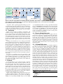
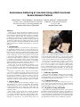
Figure 1. Cow wearing autonomous gathering sensor node.
works to monitor cattle and calibrated behavioral models for livestock using the gathered data. Kwong et al. [6] presented a similar
system for cattle monitoring with no additional modeling. Zhang et
al. [12] presented a platform to monitor zebras called ‘ZebraNet’.
In the past few years there have been efforts to extend these
sensor networks to control free-ranging animals. Butler et al. [2]
proposed the use of wireless sensor networks for virtual fencing.
Lee et al. [7] used wireless sensor networks for bull separation.
Both use similar stimuli as autonomous gathering but achieve different goals and require different algorithms. To our knowledge,
this paper presents the first work in autonomous gathering using
wireless sensor networks.
3
Gathering Algorithm
In this section, we formalize the problem of autonomously gathering animals, provide the intuition on which we based our initial
gathering algorithm, and present the gathering algorithm consisting
of a repetitive cueing loop using only sound.
3.1
Problem Statement
We assume there are n cows with positions Pi ∈ R 2 for i ∈
{1..n}. We are given a goal position Pg ∈ R 2 where we want the
cattle to gather. The problem is to move all the animals to the goal
location such that ∥Pi − Pg ∥ ≤ ε for some ε ∈ R .
3.2
Repetitive Cueing with Sound
We designed the gathering algorithm based on the experience
and intuition of animal scientists who routinely work with livestock.
The goal is to develop an automatic herding algorithm that is lowstress and natural for the animals. Humans gather animals by riding
or driving behind the group and giving voice commands. The gathering algorithm presented here tries to simulate this experience.
3‐Axis
Accelerometer
Mini SD Card
Storage
3‐Axis Magnetic 3‐Axis
Magnetic
Compass
Temperature
LPC2148
60MHz ARM7
40 KB RAM
512 KB Flash
LTC1733
Battery Circuit
512 KB
FRAM
GPS
Low‐power
FPGA
2MB Data Flash
Stereo Amplifier
2 Channel
2 Channel
24 bit DAC
FPGA
3D‐sound
2 Channel
MOSFETs
Aerocomm
AC4790
900 MHz Radio
Sensor Board
Sensor Board
Transformers for Electric Shock
Extension Board
Extension Board
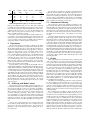
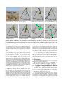
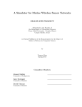
Figure 2. Overview of the platform used during gathering experiments. The extension Figure 3. Simulation of Algorithm 1.
board (right side) is usually turned off to save power. It is only activated when the sensor See Section 3.3 for a description.
board (left side) decides to cue the animal.
Algorithm 1 outlines a gathering algorithm utilizing only sound
cues. Every iteration provides an aural cue to the cow with the loop
condition ensuring that the algorithm repeats until the cow is within
ε of the goal position. The parameters tsound and twait can be random
variables to make habituation of the animals to the cues less likely.
3.3
Simulation
Figure 3 shows the results of a simulation of Algorithm 1. The
simulation was based on the behavioral model presented by Schwager et al. [10]. Schwager’s model simulates the interaction forces
between animals as well as their interaction with the environment
using parameters based on previously collected data. For the purpose of this simulation the animals’ responses to 3D sound cues was
assumed to be probabilistic. In the simulation the animals walk in
the cued direction 50% of the time and do not react to the cue otherwise.
Schwager’s model describes two forces acting upon the animal
(between animals and environment to animal). We add a third force
representing the cueing effects. The simulation weights each of
these forces by a factor to determine the absolute force acting upon
the animal. Relative to the Schwager model, we use a weight of 1.0
for the interaction force between animals and a weight of 0.4 for
the interaction force between the environment and the animal. In
determining the cueing force, no scientific data defines the relationship between applied stimuli and animal response. We specifically
choose cueing to have a higher impact than the environment, but
a lower impact than interactions between the animals, giving it a
value of 0.6.
The results of one simulation run can be seen in Figure 3. The
cows began at a random location near the middle of the paddock
and the simulation ran until the cows gathered. We performed a
total of 20 such simulation runs and in all simulations the cows
were gathered successfully within 45 minutes. This validates the
theory behind Algorithm 1.
4
Platform
For the experiments we need a platform capable of gathering
basic information such as GPS position and orientation of the cow.
The platform should offer enough computational power to run all
necessary algorithms. A radio is also required to allow continuous
real-time monitoring and remote triggering of the gathering algorithm. Further, we need the ability to cue the animals. We would
like to use two different methods: (1) a sound cueing system and
(2) an electric stimuli system. As a last requirement the platform
should be able to run continuously for at least a week to allow for
reasonable length, maintenance free, deployments.
Figure 1 shows an animal wearing our in-house developed sensor platform outlined in Figure 2. This platform provides the required functionality discussed above. It is based on the LPC2148
ARM7 processor [8] running at 60 MHz. The processor has 40 KB
of on-chip RAM and 512 KB of on-chip program flash. In addition
there is a 32 KB FRAM and a mini-SD card slot for data storage and
logging. Communication between different sensor boards and the
user is available via a 900 MHz Aerocomm AC4790 radio link. The
sensor board is equipped with all necessary sensors: temperature,
compass, accelerometers, and GPS. An expansion board provides
electric and aural cueing functionality.
4.1
Electric Stimuli Subsystem
To provide electric stimuli the board is equipped with two
drivers and two transformers to generate a high voltage. Each transformer’s power output is up to 500mW, but can be scaled by adjusting the duty cycle. The drivers are controlled by two pulse generators running inside an FPGA mounted on the expansion board.
The length of each pulse, the distance between pulses, and the total
number of pulses can be configured independently for the left and
right electric stimuli channel from the sensor board using a serial
peripheral interface.
4.2
3D Sound Subsystem
To provide sound cuing the extension board utilizes a FPGA for
3D sound processing and is further equipped with a 2 MB Data
flash to store the sound file, a 24bit stereo digital to analog sound
converter, and a stereo amplifier. We simulate directionality of the
sound by computing the running length distances between the virtual location of the sound source and the computed locations of the
cows ears. When cueing the animal aurally, the sensor board uses
the onboard accelerometer and magnetometer to continuously compute the yaw, pitch, and roll of the cow’s head. The virtual sound
source is placed at a simulated distance of 10 meters away from the
animal’s head location in the direction from which we wish to cue
the animal. Using the orientation of the cow’s head, the location of
the virtual sound source, and the assumption that the cow’s ears are
spaced by 50cm, the cpu computes the running length distances between the source and each of the cow’s ears. From this, it computes
the attenuation in percent for each ear and their relative phase difference in milliseconds. This information is computed at 20 Hz and
forwarded to the FPGA on the expansion board using a serial peripheral interface. The FPGA fetches data from a monoaural wave
file stored inside the flash. It then attenuates and appropriately delays the signal for each ear to create a stereo, directional sound. The
delay can be set between 0 to 2048 samples for each channel. Since
the sound file is recorded at 22 KHz this results in a resolution of
Algorithm 1 Repetitive Gathering Using Sound
while ∣Pcow,i − Pgoal ∣ > ε do
SOUND(tsound )
WAIT(twait )
end while
Fig.
4b
c
d
e
f
g
h
dist.
(m)
700
700
900
850
700
3000
1700
cue time
(min)
5
40
20
48
20
240
70
each cue
(sec)
30
30
30
30
60
10
10
no. cues
7
15
16
26
21
720
210
time to gather
(min)
13
55
50
no
no
no
70
Table 1. Experimental results. See Section 5.3 for details.
0.05 ms and a maximum delay of 93 ms. This delay is sufficient
to simulate the sound originating from any direction. The signal is
then synthesized using the ADC and amplifier and output on two
speakers mounted close to the cow’s ears. We measured the maximum output of each speaker at a frequency range of 1 KHz to 10
KHz to be 90dB at a distance of 10cm.
The entire system is housed inside an OtterBox 3000 case to
protect all the components from dirt and water. The electrodes and
speakers are connected using Switchcraft EN3 connectors. The sensor box is mounted on the neck of the animal with a specially designed collar that also holds the speakers and electrodes.
5
Experiments
We performed gathering experiments to validate our algorithm.
In the first set of experiments we gathered the animals by manually applying stimuli using radio control. We then performed two
autonomous gathering experiments using Algorithm 1. All experiments were performed on a group of 5 animals. Each of the 5
animals was equipped with a sensor node. However, prior to our
radio controlled gathering experiments two of the animals managed
to sever the connection between the battery at the bottom of the
collar and the sensor node at the top. As a result, during the radio controlled gathering, only 3 our of 5 animals were cued and the
GPS plots show only these 3 animals. However, we observed during the experiments that the other 2 animals remained continuously
in the group and gathered successfully.
The experiments occurred on paddocks 7B and 10B on the Jornada Experimental Range of the United States Department of Agriculture. Paddock 7B was used during the radio controlled gathering
experiments and can be seen in Figure 4(b). It has the shaped of an
isosceles triangle with sides of approximately 1500 m west and east
and 1300 m south. The corral is located at the northern tip. Paddock
10B is diamond-shaped with side lengths of approximately 2100 m
shown in Figure 4(g). The corral is located in the southern corner.
The vegetation is a Chihuahuan Semidesert Grassland [5]. It is relatively bush-free but offers the occasional obstacle to the cows in
the form of Yucca trees and mesquite. Figure 4(a) shows a sample
of the vegetation.
5.1
Gathering with Radio Control
We performed a total of 5 gathering experiments with radio control in paddock 7B between Jan. 29th and Feb. 2nd, 2009. In preparation for the experiments, we drove a boom-truck to the middle of
the paddock about 800 m south of the corral as seen in Figure 4(b).
The boom-truck served as the observatory and base station for the
researchers during the experiments. The goal was to gather and
move the animals to a corral located at the northern end of the paddock. The animals are usually moved to this location when manual
gathering is performed. For all 5 experiments the animals’ initial
start locations were between 700 m and 900 m from the goal location.
The cows were equipped with the sensor nodes the day before
the experiments started, ensuring they were not influenced by human presence when the experiments began. We performed one
gathering on each of the following 5 days at which point we removed the boxes.
For each of the 5 experiments, we began the experiment between
7:00 h and 10:45 h local time. In starting the experiment, we traveled with the base station equipment to the boom truck at least 30
minutes before starting the experiment. We chose a 30 minute interval to prevent possible influence of the scientists on the animals.
Once the experiment started, we used the base station to send aural
cuing commands to the animals over the radio.
5.2
Autonomous Gathering
We performed two autonomous gathering experiments on August 11th and 12th, 2009 in paddock 10B. Both experiments utilized Algorithm 1 presented in Section 3. We stopped the algorithm
once the animals were gathered successfully or after 4 hours, in case
gathering was not successful. In preparation for the experiments we
drove the boom-truck serving as the observatory and base station to
the middle of the north-east fence of the paddock as seen in Figure 4(g).
On August 11th we released the cows at the north end of the paddock at approximately 13:00 h. We set the sensor boxes to initiate
gathering at 14:30 h on August 11th and 8:45 h on August 12th. On
August 11th the cows were approximately 3000 m away from the
goal location while on August 12th, when the gathering algorithm
started, the animals were located in the middle of the paddock, approximately 1700 m away from the goal location. During the second experiment, the animals did not initially respond to sound cues.
While the gathering algorithm was running autonomously, we manually used the radio link to apply electrical stimuli to the animals.
Specifically, we applied this stimuli in 100 ms bursts every 20 sec
for approximately a 5 min period. After this period, the cattle began
moving and we did not interfere further with the autonomous aural
gathering algorithm.
5.3
Results
Table 1 summarizes the experimental results for gathering with
radio control (Figures 4 (b)-(e)) and autonomous gathering (Figures 4 (g)-(h)). The second column gives the animals’ approximate
distance from the goal at the beginning of the gathering experiment.
The third column is the time from the beginning of the first sound
cue to the end of the last sound cue during the experiment. The
fourth column is the length of each individual sound cue applied.
The fifth column gives the total number of cues applied during the
experiment averaged across the 3 animals. For the autonomous
gathering cues were applied every 20 seconds (0.05 Hz) resulting
in the total seen in the fifth column. The last column gives the total
time from the beginning of the experiment (first cue applied) until the animals gathered. A ’no’ means the animals did not gather
successfully in that experiment.
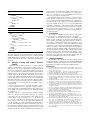
The GPS plots for all gathering with radio control experiments
are shown in Figure 4. In experiments (b), (c), and (d) the cows
were successfully gathered. In (e), the cows showed no long lasting
reactions to cueing and did not gather successfully into the corral at
all. In (f), the cows initially showed a reaction to cueing and started
walking towards the corral. However, after cueing stopped the cows
resumed foraging.
The possible reasons for failing to gather are that the cues in
(e) were not administered frequently enough and in (f) the cows
should have been cued again once they stopped gathering. Unfortunately, the radios we used during the experiments performed very
poorly offering a range of communication of only a few hundred
meters and dropping messages frequently even for distances below
100m. As a result, we were not always able to continuously cue the
animals when desired and had no feedback as to when a cue was
actually applied apart from seeing the animals reaction (though all
applied cues were recorded in log files on the sensor boxes for later
analysis). This prevented us from always being able to cue the animals when desired. We believe that the bad radio communication
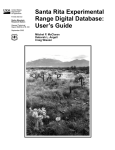
(a) Chihuahuan
Semidesert (b) Jan. 29th: 5 minutes of aural (c) Jan. 30th: Cues were sent in (d) Jan. 31st: 30 second long
Grassland landscape. Mesquite cues were applied.
multiple bursts over the course of cues were used with 5-30 second
shrub is visible in the front.
40 minutes.
pauses in between.
(e) Feb. 1st: Cued for 30 seconds (f) Feb. 2nd: Cued almost con- (g) Aug. 11th: First autonomous (h) Aug 12th:
Second auevery 60-90 seconds.
tinuously for 20 minutes.
gathering.
tonomous gathering.
Figure 4. (b)-(f): GPS plots of 3 cows during radio controlled gathering experiments. (g)-(h): GPS plots of 5 cows for autonomous gathering experiments. The boom-truck’s location is marked by a star and cues are marked by yellow dots (b-f) and
green diamonds(g-h). The corral is located at the northern (b-g) and southern (g-h) end of the paddock. In all experiments the cows
were foraging when the first cues were applied. The cows gather successfully in (a), (b), (c), and (h) and did not gather in (d), (e), and
(g).
was a significant reason for why we were not able to gather the animals in (e) and (f). We believe that the use of autonomous gathering
algorithms can help overcome this problem since radio communication is not essential once the autonomous gathering algorithm is
started.
The GPS plots for the two autonomous gathering experiments
can be seen in Figures 4 (g) and (h). In the first experiment the
cows started gathering successfully. However, during the gathering the weather changed significantly. We observed stronger winds
as well as clouds and lightning. Since cattle do not behave predictably in storms [3, 9] we attribute this failed gather to the weather
change. In Section 3.3 we explained how we simulated three forces
acting upon each animal (between animals, environment to animal,
and queuing force). We propose that changes in weather introduce
changes in the environmental force upon the animal. In the case of
our failed gather we presume that the force introduced by the lightning storm simply outweighed the force exerted by aural cueing.
The utilization of electric stimuli could possibly overcome this and
is introduced as a possible extension in Section 6.1.
In the second autonomous gathering experiment the cows did
not initially move when the gathering algorithm started cueing
them. Only after we cued the cows with electric stimuli using the
radio link did the cows start moving. However, once they were
moving no additional electrical stimuli were necessary and the cows
gather directly into the corral. Looking at the forces acting upon the
animal, the cows behavior during the second autonomous gathering
experiment suggests that the state of the animal presents a fourth
force that possibly needs to be overcome. In this model, the initial cueing with only sound did not present a strong enough force
to overcome the force exerted by the animal’s desire to remain foraging. However, once we increased the cueing force acting upon
the animal, by using electric stimuli, the animals started gathering.
This changed their state and thus the force exerted by the animals
state making it possible to gather the cows without further electric
stimuli.
It is also worth noting that the walking pattern visible on the
GPS plot is actually a path frequently utilized by the animals. Both
the reaction to changing weather and the cows adherence to an existing path are examples of how the environment plays a major role
in controlling cattle.
6
Extensions
Our results demonstrated the need for a variety of cueing mechanisms and more adaptive mechanisms.
Based on this we propose two extension of Algorithm 1: (1)
adding mild electric stimuli and (2) providing more adaptivity.
6.1
Repetitive Cueing with Sound + Electric
Stimuli
Algorithm 2 shows repetitive cueing with sound and electric
stimuli. It extends Algorithm 1, which utilized only sound cues.
If the cow is not moving after the algorithm plays a sound, the algorithm will apply electric stimuli to the cow.
In our second experiment, we would not have had to intervene
were we using Algorithm 2, suggesting that it is a better candidate
for gathering. In our first experiment, it is difficult to predict the
outcome had we used Algorithm 2. It might have provided sufficient stimulus to overcome the effect of the thunderstorm; however
Algorithm 2 Repetitive Gathering Using Sound and Electric Stimuli
while ∣Pcow,i − Pgoal ∣ > ε do
SOUND(tsound )
if cowspeed == 0 then
SHOCK(tshock )
WAIT(twait2 )
else
WAIT(twait )
end if
end while
Algorithm 3 Adaptive Gathering Using Sound and Electric Stimuli
intensity = 0.1;
while ∣Pcow,i − Pgoal ∣ > ε do
if cowspeed == 0 then
SOUND(tsound )
if intensity > 0.3 then
SHOCK(tshock , intensity)
end if
intensity = min(1.0, intensity + 0.1)
else
intensity = max(0.1, intensity − 0.1)
end if
WAIT(twait )
end while
this is not certain. This is because the behavior of cattle in a thunderstorm is difficult to predict. In such a case, continued electrical
stimuli might gather the animal or only increase its stress levels
without positive effect. The study of this relationship remains future work.
6.2
Adaptive Cueing with Sound + Electric
Stimuli
During the radio controlled gatherings, we observed that the
animals responded better to longer aural cue windows of approximately 30 seconds or longer. Algorithm 1 and Algorithm 2 should
provide cues of this length to ensure that the animals respond. However, prior observations of gathering by humans suggests that the
animals need the voice command only when they stop moving or
begin moving in the wrong direction. The animals did not need to
be cued by the humans when their heading towards the gathering
goal was approximately correct. Part of the reason is that the animals make a network of roads on their paddocks. They know where
these roads are and tend to follow roads once on them. Therefore,
once the animals are on on these paths we are less likely to need to
provide stimuli.
Based on these observations, we present Algorithm 3 as an extension to Algorithms 1 and 2. Algorithm 3 adapts cueing frequency and intensity to the animal’s behavior. The outermost loop
is responsible for stopping the cueing once the animal has reached
the goal location.
The first of the two if statements are responsible for checking
if the cow is moving. It is important to note that cowspeed is the
component of the cow’s actual speed that points towards the goal
position. If the cow is not moving (cowspeed == 0), we first cue
the cow with sound. If the cow has not been moving for a few
cycles (intensity > 0.3), then we also apply electric stimuli to the
cow. The strength of the electric stimuli increases with the value of
intensity. The variable intensity always remains in the range {0..1}.
Its value increases when the cow is not moving and decreases when
the cow is moving. This means that when the cow does not move the
strength of the electric stimulus gradually increases. Therefore, to
prevent excessive electrical electric stimuli to the animal we upper
bound intensity. If, on the other hand, the cow is moving (not
cowspeed == 0) then we do not cue the animal and decrease the
value of intensity with a lower bound of 0.
This algorithm ensures that the animal is cued only if it is not
already moving towards the goal. If it stops moving, we always
first use sound cues. If the animal habituates to the sound and does
not respond to the cue, the sound cues are reinforced with increasing electric stimuli. Both cues stop as soon as the animal starts
responding. An advantage of Algorithm 3 is that it will automatically perform long bursts of cues if the animals are not moving
given proper choices for its parameters tsound , twait , etc. We plan to
conduct autonomous gathering experiments using Algorithm 3 in
the summer of 2010.
7
Conclusion
We present a set of algorithms and experiments to gather cattle.
We provide two sets of stimuli. We performed 7 experiments.
In summary, our experiments show that to successfully gather
animals we have to take into account many environmental factors
such as weather and existing paths in the landscape. Further, we
showed that to reliably gather animals electric stimuli are necessary in addition to sound cues. Sound cues will keep the animal
going for most of the time, but electrical stimuli can help if the animal is not reacting to sound. This can happen at the beginning of
the gather because the animal is resting, such as during our second
autonomous gathering experiment. This could also happen in the
middle of a gather, such as seen in Figure 4(f). Further, our experiments demonstrated the necessity for robust and fault-tolerant
hardware because of the harsh environmental conditions (heat, dirt,
rain) and rough handling of the sensors by the animals.
8
Acknowledgments
We would like to acknowledge the following groups for their financial support: Microsoft Research, NSF, and Smarts MURI. We
would like to thank the following people for their assistance: Elizabeth Basha, Roy Libeau, Steven Proulx, and Mac Schwager.
References
[1] J. L. Albright, W. P. Gordon, W. C. Black, J. P. Dietrich, W. W. Snyder, and C. E.
Meadows. Behavioral responses of cows to auditory training. Journal of Dairy
Science, 49:104–106, 1966.
[2] Z. Butler, P. Corke, R. Peterson, and D. Rus. From robots to animals: Virtual
fences for controlling cattle. Int. J. Rob. Res., 25(5-6):485–508, 2006.
[3] M. Culley. Grazing habits of range cattle. J. For., 36:715–717, 1938.
[4] Y. Guo, G. Poulton, P. Corke, G. Bishop-Hurley, T. Wark, and D. Swain. Using
accelerometer, high sample rate gps and magnetometer data to develop a cattle
movement and behaviour model. Ecological Modelling, 220(17):2068–2075,
September 10 2009.
[5] K. Havstad, L. Huenneke, and W. Schlesinger. Structure and Function of Chihuahuan Desert Ecosystem. New York, USA: Oxford University Press, 2006.
[6] K. H. Kwong, T. T. Wu, H. G. Goh, B. Stephen, M. Gilroy, C. Michie, and
I. Andonovic. Wireless sensor networks in agriculture: Cattle monitoring for
farming industries. Progress In Electromagnetics Research Symposium, 5(1):31–
35, March 23-27 2009.
[7] C. Lee, K. C. Prayaga, A. D. Fisher, and J. M. Henshall. Behavioral aspects of
electronic bull separation and mate allocation in multiple sire mating paddocks.
Journal of Animal Science, 86:1690–1696, 2008.
[8] Phillips. LPC241x User Manual, 2 edition, July 2006.
[9] N. Rutter. Time lapse photographic studies of livestock behaviour outdoors on
the college farm aberystwyth. J. Agric. Sci., 71:257–265, 1968.
[10] M. Schwager, C. Detweiler, I. Vasilescu, D. M. Anderson, and D. Rus. DataDriven identification of group dynamics for motion prediction and control. Journal of Field Robotics, 25(6-7):305–324, 2008.
[11] B. Thorstensen, T. Syversen, T.-A. Bjørnvold, and T. Walseth. Electronic shepherd - a low-cost, low-bandwidth, wireless network system. In MobiSys ’04:
Proceedings of the 2nd international conference on Mobile systems, applications, and services, pages 245–255, New York, NY, USA, 2004. ACM.
[12] P. Zhang, C. M. Sadler, S. A. Lyon, and M. Martonosi. Hardware design experiences in zebranet. In SenSys ’04: Proceedings of the 2nd international conference on Embedded networked sensor systems, pages 227–238, New York, NY,
USA, 2004. ACM.