Download GS Amplicon Variant Analyzer

454 Sequencing System Software Manual
Version 2.9
Part D:
GS Amplicon Variant Analyzer
June 2013




For life science research only. Not for use in diagnostic procedures.
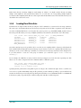
Instrument
Kit
GS Junior
Junior
GS FLX+
XL+
GS FLX+
XLR70
GS FLX
XLR70
454 Sequencing System Software Manual, v2.9
Part D: GS Amplicon Variant Analyzer
GS Amplicon Variant Analyzer
1
GS Amplicon Variant Analyzer ....................................................................................... 10
1.1 Introduction to the GS Amplicon Variant Analyzer ........................................................................... 10
1.1.1
Definitions ............................................................................................................................................................................ 10
1.1.1.1
Project ........................................................................................................................................................................ 10
1.1.1.2
Reference Sequence............................................................................................................................................ 11
1.1.1.3
Amplicon and Target ........................................................................................................................................... 11
1.1.1.4
Read Data Set and Read Group...................................................................................................................... 12
1.1.1.5
Variant ....................................................................................................................................................................... 12
1.1.1.6
Sample ....................................................................................................................................................................... 13
1.1.1.7
MID and MID Group ............................................................................................................................................ 14
1.1.1.8
Multiplexer ............................................................................................................................................................... 15
1.1.1.9
Blueprints ................................................................................................................................................................. 16
1.1.2
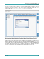
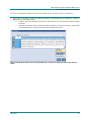
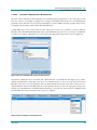
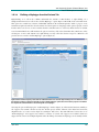
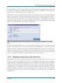
Launching the GS Amplicon Variant Analyzer GUI Application ................................................................... 16
1.1.3
GS Amplicon Variant Analyzer Application Interface Overview .................................................................... 19
1.1.3.1
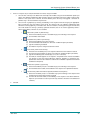
Main Buttons .......................................................................................................................................................... 20
1.1.3.2
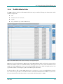
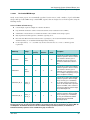
The Tabs and Sub-Tabs ..................................................................................................................................... 21
1.1.3.3
Buttons and Plots .................................................................................................................................................. 23
1.1.3.3.1 Scroll Bars .......................................................................................................................................................... 24
1.1.3.3.2 Navigation Buttons ......................................................................................................................................... 24
1.1.3.3.3 Mousing Functions ......................................................................................................................................... 25
1.1.3.3.4 Progress bars .................................................................................................................................................... 26
1.1.3.3.5 Special Action Buttons.................................................................................................................................. 26
1.1.3.4
File Browsing in Linux ......................................................................................................................................... 27
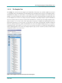
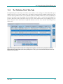
1.2 The Overview Tab ..................................................................................................................................... 27
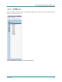
1.3 The Project Tab ......................................................................................................................................... 28
1.3.1
The “Project Tree” Sub-Tabs ........................................................................................................................................ 31
1.3.1.1
The References Tree ............................................................................................................................................ 37
1.3.1.2
The Read Data Tree ............................................................................................................................................. 38
1.3.1.3
The Samples Tree ................................................................................................................................................. 41
1.3.1.4
The MIDs Tree ........................................................................................................................................................ 42
1.3.2
The “Definition Table” Sub-Tabs ................................................................................................................................ 43
1.3.2.1
The References Definition Table .................................................................................................................... 49
1.3.2.1.1 To Enter or Edit the DNA Sequence of a Reference Sequence ................................................... 50
1.3.2.2
The Amplicons Definition Table ...................................................................................................................... 51
1.3.2.2.1 To Enter or Edit the Reference Sequence to which an Amplicon is associated ................... 52
1.3.2.2.2 To Enter or Edit the Primer Sequences for the Amplicon .............................................................. 52
1.3.2.2.3 To Enter or Edit the Target Start and End Positions ......................................................................... 53
1.3.2.3
The Read Data Definition Table ...................................................................................................................... 56
1.3.2.3.1 To Edit the Read Group of a Read Data Set ........................................................................................ 57
1.3.2.3.2 To Edit the Blueprint Associated with a Read Data Set .................................................................. 57
1.3.2.3.3 To Edit the “Active” Status of a Read Data Set................................................................................... 57
1.3.2.4
The Samples Definition Table .......................................................................................................................... 58
1.3.2.5
The Variants Definition Table ........................................................................................................................... 59
1.3.2.5.1 To Enter or Edit the Reference Sequence to which a Variant is associated .......................... 60
1.3.2.5.2 To Enter or Edit the Pattern of a (Known) Variant ............................................................................. 61
1.3.2.5.3 To Edit the Status of a Variant ................................................................................................................... 64
1.3.2.6
The MIDs Definition Table ................................................................................................................................ 66
June 2013
3
454 Sequencing System Software Manual, v2.9
Part D: GS Amplicon Variant Analyzer
1.3.2.6.1 Pre-Loaded MID Groups .............................................................................................................................. 67
1.3.2.6.2 To Enter or Edit the DNA Sequence of an MID .................................................................................. 69
1.3.2.6.3 To Edit the MID Group of an MID ............................................................................................................ 69
1.3.2.7
The Multiplexers Definition Table .................................................................................................................. 71
1.3.2.7.1 Pre-Loaded Prototype Multiplexers ......................................................................................................... 72
1.3.2.7.2 To Enter or Edit the Sample Encoding using Multiplexers ............................................................ 73
1.3.2.7.2.1 “Primer 1 MID” and “Primer 2 MID” Encoding ............................................................................ 74
1.3.2.7.2.2 “Both” Encoding ....................................................................................................................................... 74
1.3.2.7.2.3 “Either” Encoding ..................................................................................................................................... 75
1.3.2.7.3 To Enter or Edit the Primer 1 MIDs and Primer 2 MIDs .................................................................. 75
1.3.2.7.4 To Enter or Edit the Samples Assignment ............................................................................................ 78
1.3.2.7.4.1 Sample Assignment with “Primer 1 MID” or “Primer 2 MID” Encoding ........................... 79
1.3.2.7.4.2 Sample Assignment with “Both” Encoding ................................................................................... 82
1.3.2.7.4.3 Sample Assignment with “Either” Encoding................................................................................. 84
1.3.2.7.5 Using Multiplexers for more than one Read Data............................................................................. 87
1.3.2.8
The Blueprints Definition Table....................................................................................................................... 88
1.3.2.8.1 Pre-Loaded Sequence Blueprints ............................................................................................................ 88
1.3.2.8.2 Associate a Blueprint with a Read Data File ....................................................................................... 90
1.3.2.8.3 Define a Custom Blueprint .......................................................................................................................... 91
1.3.2.8.4 Sequence Blueprint Parameters ............................................................................................................... 92
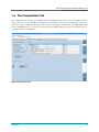
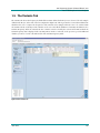
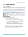
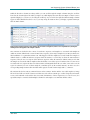
1.4 The Computations Tab ............................................................................................................................ 93
1.4.1
Variant/Consensus Computation Parameters ....................................................................................................... 94
1.4.2
Computation Speed (CPUs).......................................................................................................................................... 95
1.4.3
Project Computation ........................................................................................................................................................ 96
1.4.4
Computation Errors .......................................................................................................................................................... 98
1.5 The Variants Tab ..................................................................................................................................... 100
1.5.1
The Variants Frequency Table ................................................................................................................................... 101
1.5.1.1
General Organization......................................................................................................................................... 101
1.5.1.2
Organizing Data in the Variants Frequency Table ................................................................................ 103
1.5.1.2.1 Sort options ..................................................................................................................................................... 105
1.5.1.2.2 Ignore filters .................................................................................................................................................... 106
1.5.1.2.3 Show filters ...................................................................................................................................................... 106
1.5.1.2.4 Option reversions .......................................................................................................................................... 107
1.5.1.3
Populating the Global Align Tab from the Variants Tab ..................................................................... 107
1.5.1.4
Defining a Haplotype from the Variants Tab ........................................................................................... 108
1.5.1.5
Editing/Removing Variants from the Variants Tab ................................................................................ 109
1.5.1.6
The Mouse Tracker ............................................................................................................................................ 110
1.5.2
Variant Data Display Controls.................................................................................................................................... 111
1.5.2.1
The Alignment Read Type Controls ............................................................................................................. 111
1.5.2.2
The Show Values Controls .............................................................................................................................. 112
1.5.2.3
The Min / Max Filters ........................................................................................................................................ 113
1.5.2.4
The Variant Status Filter ................................................................................................................................... 114
1.5.2.5
The Compact Table Checkbox....................................................................................................................... 115
1.5.2.6
The Auto-Detected Variant Load Button .................................................................................................. 115
1.5.2.7
Variant Discovery Workflow ........................................................................................................................... 116
1.6 The Global Align Tab .............................................................................................................................. 118
1.6.1
Populating the Global Align Tab ............................................................................................................................... 119
1.6.2
The Variation Frequency Plot ..................................................................................................................................... 120
1.6.3
The Multiple Alignment Display ............................................................................................................................... 121
1.6.3.1
The Reference Sequence ................................................................................................................................. 121
June 2013
4
454 Sequencing System Software Manual, v2.9
Part D: GS Amplicon Variant Analyzer
1.6.3.2
The Multi-Alignment ......................................................................................................................................... 122
1.6.3.3
Special Function Buttons ................................................................................................................................. 125
1.6.4
Display Option Tools ...................................................................................................................................................... 128
1.6.4.1
Alignment Data .................................................................................................................................................... 128
1.6.4.2
Read Type............................................................................................................................................................... 130
1.6.4.3
Reported Frequency........................................................................................................................................... 130
1.6.4.4
Read Orientation ................................................................................................................................................. 131
1.6.5
Flow Signal Distribution View .................................................................................................................................... 132
1.7 The Consensus Align Tab ..................................................................................................................... 133
1.7.1
Consensus Reads ........................................................................................................................................................... 133
1.7.2
Populating the Consensus Align tab ...................................................................................................................... 134
1.7.3
The Variation Frequency Plot ..................................................................................................................................... 134
1.7.4
The Multiple Alignment Display ............................................................................................................................... 134
1.7.5
Display Option Tools ...................................................................................................................................................... 134
1.7.6
Flow Signal Distribution View .................................................................................................................................... 135
1.8 The Flowgrams Tab ................................................................................................................................ 135
1.8.1
Populating the Flowgrams Tab.................................................................................................................................. 137
1.8.2
The Tri-flowgram Plot.................................................................................................................................................... 137
1.8.3
Navigation on the Flowgrams Tab ........................................................................................................................... 139
2
Example Amplicon Project Design and Analysis .....................................................140
2.1 Experimental Design .............................................................................................................................. 140
2.2 Project Setup in the AVA Software ..................................................................................................... 143
2.2.1
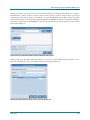
Launching the AVA Application ............................................................................................................................... 144
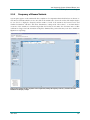
2.2.2
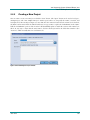
Creating a New Project ................................................................................................................................................ 145
2.2.3
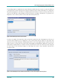
Defining the Reference Sequence ........................................................................................................................... 148
2.2.4
Defining the Amplicons................................................................................................................................................ 150
2.2.5
Defining the Sample ...................................................................................................................................................... 152
2.2.6
Defining the Known Variant ....................................................................................................................................... 153
2.2.7
Importing the Read Data Set...................................................................................................................................... 157
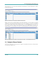
2.3 Analysis of Known Variants.................................................................................................................. 159
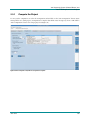
2.3.1
Compute the Project ...................................................................................................................................................... 160
2.3.2
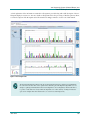
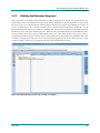
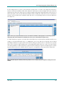
Frequency of Known Variants.................................................................................................................................... 161
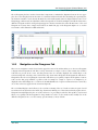
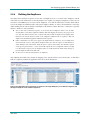
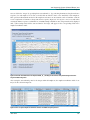
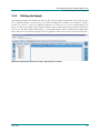
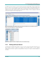
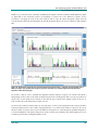
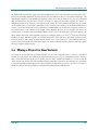
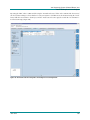
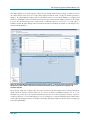
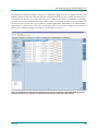
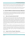
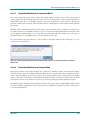
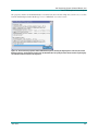
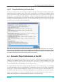
2.4 Mining a Project for New Variants...................................................................................................... 167
2.5 Important Factors in the Assessment of New Variants .................................................................. 183
2.5.1
Above the Noise .............................................................................................................................................................. 183
2.5.2
Coverage............................................................................................................................................................................. 183
2.5.3
Bidirectional Support ..................................................................................................................................................... 183
2.5.4
Homopolymers ................................................................................................................................................................. 183
2.5.5
Flowgram Evidence ........................................................................................................................................................ 184
2.5.6
Read Length ...................................................................................................................................................................... 184
2.6 Other Issues of Special Interest .......................................................................................................... 184
2.6.1
What Does ‘Sample’ Mean? ....................................................................................................................................... 184
2.6.2
How Should Your Project Be Organized? ............................................................................................................. 185
2.6.3
Should Amplicons Share a Reference Sequence or Have Individual Ones? ......................................... 186
2.6.4
When should MIDs be used? .................................................................................................................................... 186
2.6.5
What is the purpose of Multiplexers? .................................................................................................................... 187
2.6.5.1
Non-Multiplexer Example ................................................................................................................................ 187
2.6.5.2
Multiplexer Example .......................................................................................................................................... 190
2.6.5.3
Multiplexer Benefits Summary ...................................................................................................................... 192
June 2013
5
454 Sequencing System Software Manual, v2.9
Part D: GS Amplicon Variant Analyzer
3
GS Amplicon Variant Analyzer Command Line Interface ......................................193
3.1 Purpose of the CLI .................................................................................................................................. 193
3.1.1
Data Import........................................................................................................................................................................ 193
3.1.2
Data Export ........................................................................................................................................................................ 193
3.1.3
Automating the Triggering of Computations ...................................................................................................... 194
3.1.4
Result Reporting .............................................................................................................................................................. 194
3.2 AVA-CLI Command Language Overview........................................................................................... 194
3.2.1
Entities ................................................................................................................................................................................. 195
3.2.2
Available Commands ..................................................................................................................................................... 195
3.3 AVA-CLI General Online Help .............................................................................................................. 196
3.3.1
Help ...................................................................................................................................................................................... 197
3.3.2
General Help ..................................................................................................................................................................... 197
3.3.2.1
Command Line Help .......................................................................................................................................... 198
3.3.2.2
Parsing Help .......................................................................................................................................................... 200
3.3.2.3
Tabular Commands Help ................................................................................................................................. 202
3.3.2.4
Record Names Help ........................................................................................................................................... 205
3.3.2.5
Abbreviations Help ............................................................................................................................................. 206
3.3.2.6
File Paths Help...................................................................................................................................................... 207
3.3.2.7
Multiplexing Help ................................................................................................................................................ 209
3.4 AVA-CLI Command Usage Statements ............................................................................................. 210
3.4.1
associate ............................................................................................................................................................................. 210
3.4.2
close ..................................................................................................................................................................................... 215
3.4.3
computation ...................................................................................................................................................................... 215
3.4.3.1
computation start ................................................................................................................................................ 215
3.4.3.2
computation stop ................................................................................................................................................ 215
3.4.3.3
computation status ............................................................................................................................................. 216
3.4.3.4
computation loadDetectedVariants ............................................................................................................. 216
3.4.4
create ................................................................................................................................................................................... 216
3.4.4.1
create amplicon ................................................................................................................................................... 217
3.4.4.2
create blueprint.................................................................................................................................................... 219
3.4.4.3
create mid .............................................................................................................................................................. 222
3.4.4.4
create midGroup.................................................................................................................................................. 223
3.4.4.5
create multiplexer ............................................................................................................................................... 224
3.4.4.6
create project ........................................................................................................................................................ 225
3.4.4.7
create readGroup ................................................................................................................................................ 226
3.4.4.8
create reference .................................................................................................................................................. 226
3.4.4.9
create sample ....................................................................................................................................................... 227
3.4.4.10
create variant ........................................................................................................................................................ 228
3.4.5
dissociate ........................................................................................................................................................................... 229
3.4.6
exit ......................................................................................................................................................................................... 232
3.4.7
list .......................................................................................................................................................................................... 232
3.4.7.1
list amplicon .......................................................................................................................................................... 233
3.4.7.2
list blueprint........................................................................................................................................................... 234
3.4.7.3
list mid ..................................................................................................................................................................... 235
3.4.7.4
list midGroup ........................................................................................................................................................ 235
3.4.7.5
list multiplexer ...................................................................................................................................................... 236
3.4.7.6
list parameter ........................................................................................................................................................ 236
3.4.7.7
list project ............................................................................................................................................................... 237
3.4.7.8
list readData .......................................................................................................................................................... 237
3.4.7.9
list readGroup ....................................................................................................................................................... 238
June 2013
6
454 Sequencing System Software Manual, v2.9
Part D: GS Amplicon Variant Analyzer
3.4.7.10
list reference ......................................................................................................................................................... 238
3.4.7.11
list sample .............................................................................................................................................................. 239
3.4.7.12
list variant ............................................................................................................................................................... 239
3.4.8
load ....................................................................................................................................................................................... 240
3.4.9
open ...................................................................................................................................................................................... 242
3.4.10 parameter ........................................................................................................................................................................... 243
3.4.11 remove ................................................................................................................................................................................. 244
3.4.11.1
remove amplicon ................................................................................................................................................. 245
3.4.11.2
remove blueprint ................................................................................................................................................. 245
3.4.11.3
remove mid ............................................................................................................................................................ 246
3.4.11.4
remove midGroup ............................................................................................................................................... 246
3.4.11.5
remove multiplexer ............................................................................................................................................. 247
3.4.11.6
remove readData ................................................................................................................................................. 247
3.4.11.7
remove readGroup .............................................................................................................................................. 247
3.4.11.8
remove reference ................................................................................................................................................ 248
3.4.11.9
remove sample ..................................................................................................................................................... 248
3.4.11.10 remove variant ...................................................................................................................................................... 249
3.4.12 rename ................................................................................................................................................................................ 249
3.4.12.1
rename amplicon ................................................................................................................................................ 250
3.4.12.2
rename blueprint ................................................................................................................................................. 250
3.4.12.3
rename mid............................................................................................................................................................ 251
3.4.12.4
rename midGroup ............................................................................................................................................... 251
3.4.12.5
rename multiplexer............................................................................................................................................. 251
3.4.12.6
rename project ..................................................................................................................................................... 252
3.4.12.7
rename readData ................................................................................................................................................ 252
3.4.12.8
rename readGroup ............................................................................................................................................. 252
3.4.12.9
rename reference ................................................................................................................................................ 252
3.4.12.10 rename sample .................................................................................................................................................... 253
3.4.12.11 rename variant ..................................................................................................................................................... 253
3.4.13 report.................................................................................................................................................................................... 253
3.4.13.1
report alignment .................................................................................................................................................. 254
3.4.13.2
report variantHits................................................................................................................................................. 262
3.4.14 save ....................................................................................................................................................................................... 263
3.4.15 set .......................................................................................................................................................................................... 263
3.4.15.1
set verbose ............................................................................................................................................................. 263
3.4.15.2
set onErrors ........................................................................................................................................................... 264
3.4.15.3
set currDir .............................................................................................................................................................. 264
3.4.15.4
set outputFileOverwritePolicy......................................................................................................................... 265
3.4.16 show ..................................................................................................................................................................................... 265
3.4.16.1
show environment .............................................................................................................................................. 266
3.4.17 update .................................................................................................................................................................................. 266
3.4.17.1
update amplicon.................................................................................................................................................. 267
3.4.17.2
update blueprint .................................................................................................................................................. 269
3.4.17.3
update mid ............................................................................................................................................................. 272
3.4.17.4
update midGroup ................................................................................................................................................ 273
3.4.17.5
update multiplexer .............................................................................................................................................. 274
3.4.17.6
update project ...................................................................................................................................................... 275
3.4.17.7
update readData.................................................................................................................................................. 275
3.4.17.8
update readGroup .............................................................................................................................................. 276
3.4.17.9
update reference ................................................................................................................................................. 276
3.4.17.10 update sample ...................................................................................................................................................... 277
June 2013
7
454 Sequencing System Software Manual, v2.9
Part D: GS Amplicon Variant Analyzer
3.4.17.11 update variant....................................................................................................................................................... 278
3.4.18 utility ..................................................................................................................................................................................... 279
3.4.18.1
utility validateNames ......................................................................................................................................... 280
3.4.18.2
utility validateForComputation ....................................................................................................................... 281
3.4.18.3
utility makeSetupScript ..................................................................................................................................... 281
3.4.18.4
utility clone............................................................................................................................................................. 282
3.4.18.5
utility execute ........................................................................................................................................................ 283
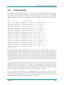
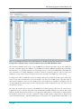
3.5 Creating and Computing a Project with the AVA-CLI .................................................................... 284
3.5.1
Setting CLI Parameters ................................................................................................................................................. 284
3.5.2
Creating a New Project ................................................................................................................................................ 285
3.5.3
Creating References ...................................................................................................................................................... 286
3.5.4
Creating Amplicons ....................................................................................................................................................... 289
3.5.5
Creating Variants ............................................................................................................................................................ 290
3.5.6
Creating Samples ............................................................................................................................................................ 291
3.5.7
Associating Samples with Amplicons .................................................................................................................... 292
3.5.8
Loading Read Data Sets .............................................................................................................................................. 293
3.5.9
Associating Read Data Sets with Samples........................................................................................................... 294
3.5.10 Editing Object Properties ............................................................................................................................................. 295
3.5.10.1
Updating an Object ............................................................................................................................................ 296
3.5.10.2
Renaming an Object .......................................................................................................................................... 296
3.5.10.3
Removing an Object .......................................................................................................................................... 296
3.5.10.4
Dissociating Relationships .............................................................................................................................. 297
3.5.11 Computation ..................................................................................................................................................................... 298
3.5.11.1
Validating the Project Before Computation ............................................................................................. 298
3.5.11.2
Managing the Computation ........................................................................................................................... 299
3.5.11.3
Loading Automatically Detected Variants ................................................................................................ 300
3.5.12 Reporting ............................................................................................................................................................................ 300
3.5.13 Finishing Touches ........................................................................................................................................................... 301
3.5.13.1
save ........................................................................................................................................................................... 301
3.5.13.2
close ......................................................................................................................................................................... 301
3.5.13.3
exit ............................................................................................................................................................................. 301
3.5.14 Exporting from the Project .......................................................................................................................................... 302
3.5.14.1
utility makeSetupScript ..................................................................................................................................... 302
3.5.14.2
utility clone............................................................................................................................................................. 302
3.5.14.3
list .............................................................................................................................................................................. 303
3.5.15 Integrated Project Script .............................................................................................................................................. 304
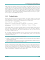
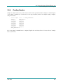
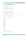
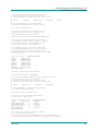
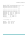
3.6 Creating and Computing an MID Project with the AVA-CLI ......................................................... 308
3.6.1
Example MID Project Script ........................................................................................................................................ 311
4
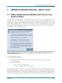
GS Amplicon Variant Analyzer – Special Topics......................................................314
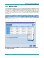
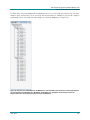
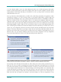
4.1 Addressing Simultaneous Multiple Users’ Access to an Amplicon Project .............................. 314
4.2 Intelligent Variant Naming ................................................................................................................... 316
4.2.1
Tier 1 Naming ................................................................................................................................................................... 316
4.2.2
Tier 2 Naming ................................................................................................................................................................... 317
4.2.3
Tier 3 Naming ................................................................................................................................................................... 318
4.2.4
Tier 4 Naming ................................................................................................................................................................... 318
4.2.5
Naming Example ............................................................................................................................................................. 318
4.3 Properties Windows for Global and Consensus Alignments ......................................................... 319
4.3.1
When is the Properties Information Useful? ........................................................................................................ 319
4.3.2
Content of the Three “Properties” Window Types ............................................................................................. 319
June 2013
8
454 Sequencing System Software Manual, v2.9
Part D: GS Amplicon Variant Analyzer
4.3.2.1
4.3.2.2
4.3.2.3
Properties Window for a Consensus Read ............................................................................................... 320
Properties Window for a Forward Read ..................................................................................................... 320
Properties Window for a Reverse Read ..................................................................................................... 322
4.4 Automatic Project Initialization in the GUI ....................................................................................... 322
4.4.1
Default Initialization Script Location ....................................................................................................................... 323
4.4.2
Default Initialization Script Contents ...................................................................................................................... 323
4.4.2.1
Steps 1 - 4: Pre-Loading MID Groups and Prototype Multiplexers ............................................... 324
4.4.2.2
Step 5: Pre-Loading Sequence Blueprints ............................................................................................... 324
4.4.2.3
Step 6: Running User-Customized Initialization Functions ............................................................... 324
4.4.3
Initialization Script Restrictions ................................................................................................................................. 325
4.4.4
Initialization Script Error Handling ........................................................................................................................... 325
4.5 Project Initialization and the CLI ......................................................................................................... 325
4.6 Multiplex Amplicon Libraries ............................................................................................................... 326
4.6.1
Basic Amplicon Design ................................................................................................................................................ 326
Glossary.....................................................................................................................................328
Index ..........................................................................................................................................331
June 2013
9
454 Sequencing System Software Manual, v2.9
Part D: GS Amplicon Variant Analyzer
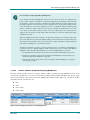
1
GS AMPLICON VARIANT ANALYZER
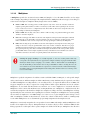
 This section describes the GS Amplicon Variant Analyzer (AVA) application through its
Graphical User Interface (GUI). The AVA software also features a Command Line Interface (CLI)
that may be more appropriate for large Projects, especially when large amounts of data need to be
imported into, exported from, or automated within a Project. See section 3 for a full description of
the CLI, the language that was developed for it, and all the commands it includes.
 Projects are compatible with each other regardless of whether they are set up or computed using
the Graphical User Interface (GUI) or the Command Line Interface (CLI). For certain projects,
some may find it useful to set up portions of the project definition using the CLI and then enter
the GUI for all subsequent tasks.
The sequencing results of Amplicon libraries are designed primarily to identify and quantitate both known and
novel DNA Variants (e.g. rare alleles) by the Ultra Deep Sequencing coverage of one or more region(s) of interest.
This is supported by the “GS Amplicon Variant Analyzer” (AVA) software described in this section.
Briefly, the AVA application computes the alignment of reads from Amplicon libraries obtained on the GS Junior or
GS FLX+ Instrument, and identifies differences between the reads and a reference sequence. Variations are displayed
both graphically with a histogram indicating positions of variation, and textually with a color-coded multiple
alignment that emphasizes regions and bases of difference from the reference sequence.
The software specifically reports the frequency of user-defined and software-identified Variants in a summary Table,
allowing for the high-throughput detection and quantitation of known and Putative Variants in the samples
sequenced. In addition, various tools and views allow the user to examine the read alignments in detail to assess
whether the software-identified Variants appear to be legitimate, and possibly identify new ones. The user can then
define these new Variants into the system, and decide which Variants to include in the analysis for quantitative
reports.
1.1 Introduction to the GS Amplicon Variant Analyzer
1.1.1
Definitions
A few important terms have special meanings or characteristics in the context of the AVA software. These are
defined and described below.
1.1.1.1
Project
An Amplicon Project is the main container of an Amplicon Sequencing experiment. In it, you specify the Reference
Sequence(s) to which the sequencing reads will be compared, in search for Variants; the Amplicon(s) that constitute
the library(ies) you sequenced [and hence, the reads in the Read Data Set(s)]; the Variant(s) that you specifically
June 2013
10
454 Sequencing System Software Manual, v2.9
Part D: GS Amplicon Variant Analyzer
want the software to search and report on; and the Sample(s) that constitute the organizational basis for the analysis.
If the Amplicon library(ies) contain Multiplex Identifiers (MIDs), the Project should further specify the MIDs used
and Multiplexers to define the relationship between MIDs and Samples. All these terms correspond to “elements”
that constitute the Amplicon Project, and are further defined in the following sub-sections. The Project format
allows the user to incrementally add new information (Read Data Sets, of course, but also Sample, Amplicon,
Variant and even new Reference Sequence or MID/Multiplexer definitions) to a Project, e.g. as the sequencing
results from new runs/regions become available.
1.1.1.2
Reference Sequence
The basic definition of a Reference Sequence is quite straightforward: it is simply a string of A, T, G, C (or N)
characters representing a DNA sequence against which the sequencing reads will be aligned and compared so
variations can be identified and reported. The Reference Sequence(s) also provide the coordinates used to localize
other elements defined in the Project (Amplicons and Variants; each Reference Sequence starts at coordinate “1”).
You can define any number of Reference Sequences in a Project.
It is important to note that only “nucleotide” characters (A, T, G, C, or N) are accepted when you enter a Reference
Sequence into the AVA software (by typing or pasting). For convenience, when pasting sequences, characters that
are not nucleotide characters and are also not IUPAC ambiguity characters (such as R for purine, Y for pyrimidine,
etc.) are removed from the pasted entry. This is useful when pasting sequences from sources that may include nonsequence information (such as white space or numerical position information in the margin of each line). During
such pastes, any IUPAC ambiguity characters are converted to “N” characters, as the other ambiguity characters are
not supported by the software (typing individual “ambiguity” characters, however, does not result in their
conversion to “N”; these are simply ignored and the text “Only ATGC and N” at the top of the Edit Sequence
window turns bold and red to alert you that an invalid character was used). The restriction that no ambiguity
characters other than N be present in a sequence is a requirement of many alignment algorithms and is not unique
to the 454 Sequencing system software.
It is also important to be aware that shorter Reference Sequences are more efficient for computation in the AVA
software, whereas a long Reference Sequence could result in unnecessarily long computation times and slow
navigation and scrolling in the application’s windows. Since in Amplicon sequencing, the interest is in one or a few
small regions of DNA, the user should specify such region(s) when defining the Reference Sequence(s) for a Project
rather than entering, for example, the entire genome of the organism. If you want to monitor together multiple
targets that are distant from one another in the reference genome (for example exons of a given gene), you can create
an “artificial” Reference Sequence by concatenating the segments of interest; it is useful to insert a few “N” characters
between the concatenated targets if you create artificial Reference Sequences.
1.1.1.3
Amplicon and Target
The term Amplicon is used in the AVA software to represent essentially the same entity (sequence) as in the
preparation of an Amplicon library, except that it does not include the 19 bp “Primer A” and “Primer B” parts of the
Fusion Primers. As such, therefore, they match the sequencing reads from the Read Data Set(s).
In the AVA software, however, an Amplicon is a virtual entity defined relative to a Reference Sequence by specifying
two primers (the “template-specific” parts of the Fusion Primers). This relative definition is also directional: the
June 2013
11
454 Sequencing System Software Manual, v2.9
Part D: GS Amplicon Variant Analyzer
AVA software names the two template-specific primers “Primer 1” and “Primer 2” in the 5’-Primer 1 --> Primer 2-3’
orientation of the Reference Sequence. Therefore, Amplicon orientation is internal to the AVA software, and is NOT
dependent upon the “Primer A” and “Primer B” parts of the Fusion Primers used in library construction.
You can define any number of Amplicons in a Project, each associated with a specific Reference Sequence; you can
also associate multiple Amplicons, even overlapping ones, with a given Reference Sequence. Thus, a Reference
Sequence may be associated with multiple Amplicons, but an Amplicon may only be associated with one Reference
Sequence. Amplicons are also associated with Read Data Sets and with Samples (see below).
The term Target specifies the part of an Amplicon that is between the two primers (i.e., the non-primer portion of
the Amplicon). This is the sequence that is actually aligned to the Reference Sequence during the computations. It is
important to trim the primers before alignment because any Variant found therein would be a reflection of primer
design (or errors in primer synthesis) rather than representing variations in the DNA sample used to prepare the
Amplicon library, and therefore would not have any biological significance.
1.1.1.4
Read Data Set and Read Group
A Read Data Set is a group of sequencing reads derived from an Amplicon library. In a Project, Read Data Sets exist
within a Read Group (this helps to organize the data) and are associated with pairings of Amplicons and Samples:

the Amplicon association specifies which Amplicon(s) were included in the sequencing run that produced
this Read Data Set; the reads are identified as belonging to an Amplicon by virtue of their template-specific
primers (see section 1.1.1.3, above)

the Sample association specifies in which Sample(s) to report the results of the computations (see section
1.1.1.6, below, for a more detailed explanation of “Samples”).
You can include any number of Read Data Sets in a Project; and associate them with any number of AmpliconSample pairs. However, an Amplicon cannot be associated with more than one Sample within a given Read Data Set
unless MIDs are used to further associate the reads with specific Samples; see section 1.1.1.7 for more details on this.
Note also that the AVA software can only process reads from Amplicon libraries.
In the current release of the AVA software, a Read Data Set is equivalent to an SFF file, e.g. as output by the data
processing pipeline of the 454 Sequencing system, each file corresponding to a region of the PTP device. On the GS
Junior system, there is only one region per run while on the GS FLX+ system, there can be two or more regions per
run depending on the gasket format employed. Using sffile (see Part C of this manual) from the command line, a
user may reorganize the SFF files into multiple separate files prior to importing them as Read Data Sets into a
Project, as long as all of the SFF files to be merged share the same flow pattern and flow list. More typically, the SFF
files are taken as-is from the data processing pipeline and so for the GS Junior system, there will typically be one
Read Data Set for each Amplicon sequencing run you import into the Project, and for Amplicon Sequencing
performed on a GS FLX+ system, there will usually be one Read Data set for each region of the PTP device of the run
you import
1.1.1.5
Variant
Simply put, a Variant is a sequence difference relative to a Reference Sequence. Like Amplicons, Variants are thus
defined relative to a Reference Sequence. Four kinds of variations can be defined in the AVA software: substitutions,
June 2013
12
454 Sequencing System Software Manual, v2.9
Part D: GS Amplicon Variant Analyzer
deletions, insertions, and required matches; and a Defined Variant can include any number of these, in any
combination (haplotypic variations). You can define any number of Variants in a Project, each associated with a
specific Reference Sequence; you can also associate any number of Variants to a given Reference Sequence.
Though the multiple alignment views of the AVA software show all variations between the reads displayed and their
Reference Sequence, a Variant must be defined in the Project to be reported in the application’s Variants tab. Known
Variants (e.g. from the scientific literature) can be defined directly in a Project, and Putative substitution and
deletion Variants will be automatically identified and defined by the AVA software if they are detected at a preset
minimum abundance during computation of the Project; alignments of these Putative Variants can be examined in
detail, to allow you to formally “accept” them as legitimate Variants or “reject” them as noise. You can also define
new Variants from the variations observed between the Reference Sequence(s) and the reads included in your
Project.
The Variants tab thus reports statistics on the observed incidence (in all the reads included in the last computation
of the Project) of each Defined Variant, broken out by Sample. A Variant’s definition specifies one or more
Reference Sequence positions whose nucleotide identity must be matched or mutated in some way. Only reads that,
in their multiple alignment to the Reference Sequence, span the entire set of Variant positions are eligible to
contribute to the statistics computed for that Variant.
1.1.1.6
Sample
The term Sample, in the context of the AVA software, can be defined very generically as a virtual “container”
specified by the user only as a name (and an optional annotation), and used to group reads for analysis and
reporting. The Samples thus represent the organizational foundation for the analysis, whose primary output is the
Variants Tab, such that the frequency of any or all Defined Variants can be compared between the different
“Samples” defined in the Project. You can define any number of Samples in a Project, each associated with one or
more Read Data Sets and with one or more Amplicons. For example, Samples could correspond to sequencing data
from an Amplicon library prepared from a “control” DNA sample; and those associated with a second Sample, to a
library prepared from the DNA of an “experimental” tissue or individual. Or, different Samples could correspond to
multiple replicate libraries of a biological sample, e.g. to allow for statistical comparison between them.
Within a Read Data Set, reads may correspond to one or more Samples. In order to demultiplex the reads, i.e. assign
them each to the proper Sample, the reads must contain reliably identifiable Sample-specific features. The AVA
software can use either of two mechanisms to assign reads to Samples:
1.
It can use the known template-specific part of the Adaptor used to prepare the Amplicon library. This works well when
the Amplicon identity alone is sufficient to assign the reads to Samples; this restricts one to the case where any given
Amplicon within a Read Data Set provides reads for only one Sample (though it allows reads from different Amplicons
to belong to the same Sample.)
2.
It can use Multiplex Identifiers (MIDs) in conjunction with the template-specific part of the Adaptor. This is required if
reads from a given Amplicon need to be assigned to more than one Sample in the same Read Data Set; the MIDs then
provide the additional context necessary to resolve the reads to the appropriate Samples.
To perform the read to Sample assignments, the AVA software relies on user-specified, three-way associations
between Read Data Sets – Samples – Amplicons (first mechanism), or Read Data Sets – Multiplexers – Amplicons
June 2013
13
454 Sequencing System Software Manual, v2.9
Part D: GS Amplicon Variant Analyzer
(second mechanism). In the second case, the Multiplexers (see sections 1.1.1.7 and 1.1.1.8) provide the MID to
Sample assignment information. Within one Read Data Set, a given Amplicon cannot belong to more than one such
three-way association because the software would then be unable to unambiguously determine which association
mechanism to use in order to assign reads from that Amplicon to their proper Samples.
Once the read to Sample assignment is made, the AVA software can compute the prevalence of Variants found in
the reads, broken out by Sample. These statistics are reported in the Variants tab (section 1.5). Be aware, however,
that while you can examine Variant frequency statistics for all the Samples of the Project in the Variants tab, you can
view read alignments of only one Sample at a time (e.g. in the Global Align tab).
1.1.1.7
MID and MID Group
An MID (or Multiplex Identifier) is a short, recognizable sequence tag that can be added to the design of the
Adaptors used for library preparation, between the sequencing key and the template-specific primer, to help
determine the provenance of the read (see section 4.6). Multiple Amplicon libraries (the Project’s Samples) can be
prepared that include the same Amplicon target sequences (with the same template-specific primers), each labeled
with different MID tags. The MID sequences provide extra context that, in concert with the template-specific
primers, allow flexible demultiplexing options, and specifically enable the sequencing of the same Amplicon across
multiple Samples within the same Read Data Set: when using MIDs, the Sample-Amplicon associations are indirectly
specified in the software by associating Amplicons with Multiplexers (see section 1.1.1.8), which themselves specify
the relationship between MIDs and Samples and then apply that information to the associated Amplicons. Note that
both non-MID and MID-tagged Amplicons may be used in a Project, but within a given Read Data Set, all the reads
for any individual Amplicon must be of one type or the other.
Contrary to the situation with Shotgun (sstDNA) libraries, where an MID sequence can only be on Adaptor A,
Amplicon libraries can be constructed with MIDs at either or both ends of the reads. This provides for considerable
flexibility in the design of the MID Amplicon libraries. In particular, if the Amplicons are designed such that the
read length of the sequencing run allows full read-through of the Amplicon reads, then placing MIDs at both ends of
the reads makes it possible to use them combinatorially, such that a small number of MID tags can encode a much
larger number of Samples (per the “Both” encoding; see section 1.1.1.8).
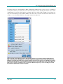
An MID Group is a set of MIDs that have been designed to work well together. The AVA software is configured to
automatically load an AVA project (created via the “New” button in the GUI) with several MID Groups that have
been carefully chosen to be resilient to sequencing and primer synthesis errors (see section 1.3.2.6.1 for details).
June 2013
14
454 Sequencing System Software Manual, v2.9
Part D: GS Amplicon Variant Analyzer
1.1.1.8
Multiplexer
A Multiplexer specifies the association between MIDs and Samples, i.e. how the MIDs should be used to assign
reads to Samples. Depending on the design of the Amplicon libraries, Multiplexers allow four types of encoding (see
section 4.6 for a description of Amplicon library design, in the context of MIDs):

Primer 1 MID: This encoding provides an MID signature only on the end of the read that contains the
template-specific primer defined as “Primer 1” in the Project. This will be at the beginning of the “forward”
reads, or at the end of “reverse” (complemented) reads. These MIDs are then used to assign the reads to the
proper Sample, as defined by the Multiplexer.

Primer 2 MID: This encoding is the same as Primer 1 MID encoding, except that the MID appears at the
“Primer 2” end of the Amplicons.

Both: This encoding provides MIDs at both ends of the Amplicons and requires that read length be sufficient
to read through to the distal MID, in both orientations. The paired combination of MIDs located on the
Primer 1 and Primer 2 sides is used to assign reads to their proper Sample, as defined by the Multiplexer.

Either: This encoding also provides MIDs at both ends of the Amplicons, but assigns the reads to their proper
Sample on the basis of only the proximal MID on the read, in either orientation. This allows for proper
assignment of both forward and reverse reads even if the Amplicon is longer than the read length provided by
the sequencing run script. Note that even if full read-through to the distal end of the read is possible, only the
proximal MID will be used for Sample assignment (and any contradiction between the MIDs seen at the two
ends will be assumed to be the effect of sequencing artifacts at the distal end of the read).
Selecting the proper encoding: It is crucially important to select the encoding method that truly
corresponds to the way the libraries were prepared. For example, if a library was prepared with the ‘Either’
chemistry in mind, it may be tempting to use a ‘Primer 1 MID’ or ‘Primer2 MID’ encoded Multiplexer
since the distal MID gets discounted in favor of the proximal MID, in ‘Either’ encoding. However, the
AVA software needs to know that MIDs are expected to be found at both ends: without that knowledge,
the trimmer might get a suboptimal alignment of the distal primer, which in certain cases could drop valid
reads out of the analysis.
Multiplexers specify the assignment of reads that contain each defined MID (or MID pair) to each specific Sample,
within a Read Data Set. Different Amplicons within a Read Data Set may simultaneously be sequenced even if they
use different Multiplexer encoding methods, or no encoding at all (i.e. are sequenced without the use of MIDs), but
any given Amplicon can only be sequenced in a single manner within a given Read Data Set. In the software,
Multiplexers are associated with Read Data Sets and then one or more Amplicons are associated with those
Multiplexers, in the context of the Read Data Sets (creating Read Data Sets – Multiplexers – Amplicons triads). The
software then assigns the reads from those Amplicons to Samples according to the rules of the Multiplexer encoding.
Operationally, the same restriction exists regarding the association of Amplicons to Multiplexers as exists regarding
the association of Amplicons to non-MID Samples (see section 1.1.1.6): a given Amplicon cannot belong to more
than one Multiplexer within one Read Data Set, because the software would then be unable to unambiguously
resolve which Multiplexer to use to determine the proper Sample assignment for the Amplicon reads.
Multiplexers conveniently encapsulate the correspondence between MIDs and Samples. Without Multiplexers, each
instance of an Amplicon in a Project, distinguished from one another only by a choice of different MIDs in their
library preparation, would require that a separate Amplicon be defined in the Project. Multiplexers also allow the
June 2013
15
454 Sequencing System Software Manual, v2.9
Part D: GS Amplicon Variant Analyzer
correspondence between MIDs and Samples to be specified only once and shared across multiple Amplicons that
may be sequenced simultaneously, a common experimental design. These and other benefits of using Multiplexers,
including the more accurate decoding of MIDs and the reduction of errors in Sample assignment during the
demultiplexing phase of computation, are further described in section 2.6.5.
1.1.1.9
Blueprints
A sequence Blueprint specifies the linear arrangement of Adaptors, universal tails, MIDs, and target specific primers
used during library preparation for an AVA project. The AVA software uses the Blueprint definition to determine
which sequences to trim away from the Amplicon sequence of interest before performing multi-alignment and
Variant calling. The ability to specify either a pre-loaded or custom Blueprint allows the AVA software to support
any library preparation chemistry that generates a target-specific sequence at the 5’ end of an Amplicon of interest.
This includes all of the experimental designs described in the 454 Sequencing System Guidelines for Amplicon
Experimental Design, with the exception of the Long Range PCR design.
 Basic Amplicon Design
 Universal Tailed Amplicon Design
 Ligated Adaptors Design
 One-Way Reads Design
1.1.2
Launching the GS Amplicon Variant Analyzer GUI Application
The GS Amplicon Variant Analyzer GUI application is launched by double clicking on its desktop icon.
From a Linux terminal window on an attendant PC or a datarig, where the data analysis software package is
installed, the following command can be used to launch the GS Amplicon Variant Analyzer GUI application:
gsAmplicon [advanced options: --cpu, --maxPerm, --maxHeap --configDir]
The gsAmplicon command supports only the “advanced options” of the command line interface (preceded by
two dashes), not the other “basic options” (preceded by a single dash). These advanced options are documented in
detail in section 3.3.2.1.
June 2013
16
454 Sequencing System Software Manual, v2.9
Part D: GS Amplicon Variant Analyzer
The “--cpu” option can accelerate computation through the use of multiple processors. The default value for
maxPerm is 256 megabytes for gsAmplicon and 128 megabytes for doAmplicon (which is used to configure a
project from the command line; see Section 3 for additional details). The default value for maxHeap is 750
megabytes for both gsAmplicon and doAmplicon. The --maxPerm and --maxHeap parameters can be used
on the command line to override the default memory allocations on a case-by-case basis. For a more permanent
configuration, edit one of the following .vmoptions files with the desired values.
/opt/454/apps/amplicons/config/gsAmplicon.vmoptions
/opt/454/apps/amplicons/config/doAmplicon.vmoptions
gsAmplicon command interruption: If you interrupt the gsAmplicon command, accidentally or
otherwise, by typing control-C, the application will immediately shutdown, not giving you a chance to
save any of your recent Project changes. For additional safety, you may prefer to start the command in the
background, ending the command line with a ‘&’, as in: “gsAmplicon &”. Other modes of exiting the
application, such as clicking the “Exit” button, would elicit warning dialogs if the Project contains any
unsaved changes.
June 2013
17
454 Sequencing System Software Manual, v2.9
Part D: GS Amplicon Variant Analyzer
This will open the AVA GUI application main window in its Overview tab (Figure 1). [A splash screen identifying
the application and its version number will be displayed briefly (not shown); you can also view this splash screen at
any time, after launching the application, by clicking on the “About” button.] Until a Project is open, the Overview
tab provides a brief textual description of the AVA application’s usage and capabilities. There are two ways to open a
Project at this point: you can create a new Project by clicking on the “New” button, or you can open an existing
Project by clicking on the “Open” button (see section 1.1.3.1). Note that if you do not have write-permission to the
Project folder, or if another user already has it open, you can open the Project as “Read-Only”, but you will be unable
to save any changes or carry out any computations (which requires writing to disk). See section 4.1 for more details
on this kind of situation.
Figure 1: The Overview tab showing the textual description of the application, before a Project is open.
June 2013
18
454 Sequencing System Software Manual, v2.9
Part D: GS Amplicon Variant Analyzer
1.1.3
GS Amplicon Variant Analyzer Application Interface Overview
The top of the main AVA window shows the name and path of the Amplicon Project being displayed; and a set of
seven main buttons are located along the right-hand side of the window. The rest of the AVA window is occupied by
a selection of tabs, described in the sections below.
 Make sure to set the resolution of your computer screen to at least 1024x768 pixels (1280x1024
recommended), or the AVA application may not be able to display all the features described
below. If the resolution is too low (or if the application window or one of its constituent tabbed
panels are resized too small), the software attempts to prioritize which feature to omit. For
example, the Global Align tab may not show the color code legend on its lower-left corner; or the
button column to the left of the Variation Frequency Plot on the top panel of the Global Align or
the Consensus Align tabs may not show the “Save plot data to spreadsheet file” and/or the “Save
plot snapshot to image file” buttons. While program features may be omitted in this way,
scrollbars are used as needed to ensure that all data is viewable regardless of the screen resolution
or window size.
 The AVA software also features a Command Line Interface (CLI) that may be more appropriate
for large Projects, especially when large amounts of data need to be imported into, exported from,
or automated within a Project. See section 3 for a full description of the CLI, the language that was
developed for it, and all the commands it includes.
June 2013
19
454 Sequencing System Software Manual, v2.9
Part D: GS Amplicon Variant Analyzer
1.1.3.1
Main Buttons
Seven main buttons are always visible, along the right-hand side of the GS Amplicon Variant Analyzer window (Save
and Back are grayed-out when their function is not applicable, e.g. no Project changes to save):
Icon
Description
The Exit button closes the AVA application.
The New button opens a “New Amplicon Project” window in which you can provide a name for a new
Project, as well as a file-system location where to save it and a free-text description (Figure 2). Clicking “OK”
in the “New Amplicon Project” window initializes the Project and takes you to the Project Tab of your new
Project. For more details on Project initialization, see section 4.4. (See section 2.2.2 for more details on ways
to create a new Project, especially synchronizing the Project and Location names, and navigating your filesystem using the “folder” icon to the right of the ‘Location’ field.)
The Open button allows you to browse your file-system to find an existing Amplicon Project and open it in
the AVA application.
The Save button saves the current state of the Project to the disk, i.e. all the primary elements and their
associations.
The Back button takes you back to the previous AVA view. (Note that this button does not carry an “undo”
function; see Note, below.)
The About button opens a splash screen providing some information about the AVA application. (Click the
“Close” button to close it).
The Help button opens an electronic version of the user manual.
The AVA software does not offer the possibility to “undo” an action such as a computation, an element
definition entry, a display selection in a multi-alignment view, etc. In some cases, the opposite action or a
“clear” action may be available. You can also revert to the last saved state of the Project by re-opening the
Project without first clicking the “Save” button.
Saving vs. computing a project: Saving a Project does NOT update the results displayed in the Variants,
Global Align, Consensus Align or Flowgrams tabs. To update these displays after making changes in a
Project, you must re-compute it. Conversely, these results do not require that you save the Project to
persist in the Project.
June 2013
20
454 Sequencing System Software Manual, v2.9
Part D: GS Amplicon Variant Analyzer
Figure 2: The New Amplicon Project window, with fields to enter a Project’s name, file-system location, and textual
description. If the “Generate location based on name” box is checked, typing a Project’s name in the Name field also enters it
at the end of the path in the Location field. Be aware that later changing the name of the Project from within the application
will NOT change the name of the folder that contains it, causing a mismatch between the two; a mismatch would also occur if
the “Generate location based on name” box is not checked, and you type different names for the Project (in the Name field)
and the folder (at the end of the path). If there is a problem with the selected location, the OK button will be disabled, the
location field will be highlighted in red, and, if you position the mouse over the location field, a screen tip will appear
indicating the nature of the problem. The button to the right of the Location field allows you to browse your file-system to set a
location path. See section 2.2.2 for an example and additional details on ways to create a new Project in the AVA software.
1.1.3.2
The Tabs and Sub-Tabs
The AVA application displays the various aspects of the Amplicon Project in a series of 7 tabs, with the Project tab
separated into two panels (themselves comprising 4 and 7 sub-tabs, respectively). When a tab has no content, its
name is grayed out and the tab is unavailable. When a tab does have content, a green square icon appears next to its
name; clicking on an available tab or sub-tab name brings the information it contains to the front for viewing, as
listed below. If the size of your screen does not allow you to view all the tabs, a pair of scroll arrow buttons in each
panel allows you to scroll the set of tabs to bring hidden ones into view. The contents and usage of the information
included in the tabs are described in full detail in sections 1.2 through 1.8.

The Overview tab provides a basic summary of the Amplicon Project.

The Project tab is used to set up the Project (define all the elements that compose it and their associations)
and to navigate it and select particular Sample-Amplicon pairs to view in the Global Align tab. The Project
tab contains two panels:


The left panel comprises 4 sub-tabs that show various representations of the Project in “tree” form,
thus displaying the associations between the various elements that compose it.

The right panel comprises 7 sub-tabs that list and show all the characteristics of the various
“elements” defined in the Project, in tabular form.
The Computations tab allows the user to control Variant calling, compute (or re-compute) the Project, and
view the progress and state of each computation step.
June 2013
21
454 Sequencing System Software Manual, v2.9
Part D: GS Amplicon Variant Analyzer

The Variants tab provides summary results of the GS Amplicon Variant Analyzer, listing the observed
frequency of each Defined Variant in each relevant Sample. A Sample is relevant to a Variant when the Read
Data Set(s) with which it is associated contain reads that cover all the Reference Sequence positions specified
in the Variant’s definition.

The Global Align tab is populated with the multiple alignment (against the appropriate Reference Sequence)
of the reads corresponding to one or more selected Sample-Amplicon pair(s). Such a selection is done by
right-clicking on an appropriate object in any of the Project Trees or in the Variants Tab (only one SampleAmplicon pair can be selected this way), or by using a navigation dialog found within the Global Align tab
itself (multiple pairs selection possible). The reads displayed may be Individual Reads, corresponding to
sequence reads directly extracted from the Read Data Set(s), or Consensus Reads, corresponding to sets of
Individual Reads that were collapsed into a single representative read (in order to simplify the display and
eliminate noise from the data). In either case, the tab comprises two data panels:

The top panel is a stacked histogram indicating the frequency of all the variations observed between
the selected reads and the Reference Sequence associated with the Amplicon(s) from which the
reads were derived. The histogram is based on a gapped multiple alignment and, thus, may contain
data for positions of the alignment that occur between positions of the Reference Sequence itself.
This graph also shows depth of coverage for each position of the alignment.

The bottom panel displays the (gapped) sequence multi-alignment of the reads, aligned below the
Reference Sequence. Color codes help to highlight variations in the reads in comparison with the
Reference Sequence; the Individual or Consensus Reads can be filtered for display to help identify
specific variations and potentially discover haplotypes.

The Consensus Align tab displays the same information as the Global Align tab, but for the set of Individual
Reads that were collapsed into a Consensus Read on the Global Align tab. A line highlighting the differences
between that Consensus Read Sequence and the Reference Sequence is displayed directly below the Reference
Sequence in the alignment.

The Flowgrams tab, finally, displays a tri-flowgram view of an individual read, selected from either the Global
Align or the Consensus Align tab. This display is designed to help evaluate the significance of differences
between an individual read and a Reference Sequence. As such, the read flowgram displayed is not the raw
flowgram of the read, but is a computationally processed version designed to facilitate the comparison of the
read flowgram with an idealized flowgram for the Reference Sequence. In particular, flowgram gaps may be
introduced into one or both flowgrams in order to optimize their alignment, and the flowgram of the read
may be computationally reverse-complemented in order that the display always be in the 5’-->3’ orientation
of the Reference Sequence. Finally, the flowgram only displays the subset of flows relevant to the read’s
sequence alignment as displayed in the Global Align or Consensus Align tabs. The display is divided into
three panels:

The top panel shows an aligned, idealized flowgram for the Reference Sequence.

The middle panel shows the aligned, (possibly reverse-complemented) flowgram of the read.

The bottom panel shows a difference flowgram (read minus reference), where any variation from
the Reference Sequence is seen as a non-zero value. Specifically, extra signals in the read, relative to
the Reference Sequence, are displayed as positive differences in this panel; and missing signals in
the read, relative to the Reference Sequence, are displayed as negative differences.
When a tab is divided into panels, the panels can be resized by dragging the separator. Also, when the panels are
stacked vertically (as in the case of the Global Align, the Consensus Align and the Flowgrams tabs), two small
buttons are present at the left edge of the separator(s); these buttons allow you to collapse one of the panels, leaving
the entire height of the window to the other one(s). This action is reversible (use the other button to re-expand the
panel).
June 2013
22
454 Sequencing System Software Manual, v2.9
Part D: GS Amplicon Variant Analyzer
1.1.3.3
Buttons and Plots
The plots, multi-alignment views and data tables displayed in the various tabs of the AVA application are scrollable
and/or zoomable graphical elements. They share certain common buttons and functions, e.g. to perform the
scrolling and zooming. When they do appear, these graphic elements have some or all of the following features (see
in Figure 3, an example for a Global Align window which has many of these elements):

Scroll bars for horizontal and/or vertical scrolling (appearing below and to the right of the element, if
necessary).

A column of buttons along the upper left edge of the graphic elements, used for navigation (including various
zooming functions) and/or to save snapshot images or text files of the displayed data.

Additional functional buttons, also in the column at the left of graphic elements, to carry out actions such as
applying a selection filter on the reads currently displayed, defining novel Variants, assembling consistent
reads (which might span overlapping Amplicons) into Consensus Reads, running a computation of the
Project, adding or removing Project elements or associations, etc.

“Mousing” functions (pointing, clicking or dragging the mouse, touchpad, pen, etc. over the graphical
element) to view data values and adjust the zoom level.

When a plot with DNA sequence information is present (Variation Frequency Plot and Flowgrams), a legend
is shown, giving the color code for the nucleotides [as well as gaps (“-”) and depth of coverage (“#”), if
appropriate].
Figure 3: An example Global Align tab showing many of the common graphical element functions.
June 2013
23
454 Sequencing System Software Manual, v2.9
Part D: GS Amplicon Variant Analyzer
1.1.3.3.1
Scroll Bars
The scroll bars have the standard functions, and appear when the data in either direction is too large to be shown in
the viewable area. In Figure 3, for example, the horizontal scrollbar appears in the multi-alignment pane, and the
vertical one appears in the plot pane; others are not displayed because axes scales are set such that the full breadth of
the data can be seen.
1.1.3.3.2
Navigation Buttons
Many of the buttons appearing to the left of an element are used for navigation on the element, and have the
following general functions:
Button
Name – Description
Fit – Fit means to scale out to the limits of the data. The y-axis is rounded to an attractive-looking number
rather than stopping at the exact data limit.
Zoom in – Zoom in by a factor of 1.5. This button zooms only the primary (left) y-axis scale; use the Zoom to
labels and Freehand zooming functions described below to zoom the x-axis.
Zoom out – Zoom out by a factor of 1.5. This button will zoom only the primary y-axis scale and, unlike other
zoom operations, this will zoom out past the data limits (to allow you to get a better perspective of the data,
especially when attempting to visually separate data on the primary and secondary y-axes).
Zoom to labels – This button zooms the x-axis of the flowgram so that the nucleotide/flow characters can fit
below the axis.
Snapshot – Save a snapshot image of the current view to disk. This will open a dialog asking for the location
and filename to save a PNG format snapshot image. The saved image contains only the currently visible region
of the element: in particular, if the element is displayed in the context of a scrollbar, only the current, scrolled
view is saved.
Text file – Save a text-formatted version of the element. This will open a dialog asking for the location and
filename to save the text file. It then saves the data, along with summary information describing the data
source. In most cases the user has the option of exporting a tab or comma-separated text file of the
underlying data element. For plots, the text file includes data that may be outside of the current view (due to
scrollbars). For a flowgram view (see section 1.8), the data for all three plots are saved to one file, with some
white space between the three sections of plot data. For summary data tables, the file contains the tabular
data, also including data that may be beyond the current scroll region. For multiple-alignment displays, seven
output formats are supported: FASTA, Clustal, Ace, SAM, BAM, and Table (csv and tsv). For the Variants Table,
finally, the text file includes an extra column (Variant Status), as compared to the Table visible in the GUI,
placed between the Variant Name and Max Value columns (i.e. at column 3 in the text output); note that
although the GUI lacks an explicit column for this, the Variant Status data is accessible via the tooltips as you
pause the mouse over Variants).
June 2013
24
454 Sequencing System Software Manual, v2.9
Part D: GS Amplicon Variant Analyzer
1.1.3.3.3
Mousing Functions
When the mouse cursor is located over a graphical element, additional functions can be performed by moving,
clicking or dragging the mouse:

Mouse Tracker – Whenever the cursor is located over a position in a plot or a multi-alignment display,
detailed data values for that position are shown in a related Mouse Tracker area, at the bottom left of the
window. This allows you to see the specific numerical value for any data point as well as other detailed data
associated with the display position.

Freehand Zoom In – The mouse can be used to zoom in on specific regions of a plot. To zoom in, hold the
left mouse button down and drag a box around the area of interest (see Figure 4). Releasing the button zooms
to the area circumscribed by the box. If the plot has both primary and secondary Y-axes, only the primary
axis data is zoomed.
↓
Figure 4: Freehand zoom in to a flowgram region.
June 2013
25
454 Sequencing System Software Manual, v2.9
Part D: GS Amplicon Variant Analyzer

Freehand zoom out – For plots only, right-clicking the plot will cause the plot to zoom out by a factor of 1.5
in both the X and (primary) Y directions, centered on the middle of the current view. This zoom will not
zoom farther than the limits of the data.

Screen tips – When you hover the mouse over a button or other display control, over an element definition
data, or over most of the Variants or multi-alignment results, a screen tip appears providing some
information about the object under the pointer. Some of the most useful examples of this are specified in the
tab sections, below.
1.1.3.3.4
Progress bars
When an operation takes more than a few seconds, a Progress bar appears temporarily in the upper-right corner of
the application window, to display the progress of the operation (Figure 5A). Double-clicking on this progress bar
opens the Progress window, which contains individual progress bars for the operation or any of its sub-processes
(Figure 5B). In certain contexts, you can cancel an operation by clicking the “Cancel” button that appears to the
right of a progress bar in the Progress Window (when cancelling is not possible, such as when new data is being
loaded, the Cancel button is present, but grayed out). The Progress window stays open, even after the entire
operation completes, until you close it manually.
A
B
Figure 5: (A) A Progress bar (B) The Progress window.
1.1.3.3.5
Special Action Buttons
Another functional category of buttons appears to the left of some graphic elements or in the display options area of
certain tabs. Since these are tab-specific, these buttons are described in the corresponding tab sections, below.
June 2013
26
454 Sequencing System Software Manual, v2.9
Part D: GS Amplicon Variant Analyzer
1.1.3.4
File Browsing in Linux
The Linux File Brower used for opening Projects, finding Read Data Sets, and creating New Projects lacks some of
the usually expected controls. For example, there are no buttons for going up a directory, creating a new folder, etc.
However, these functions can be found by right-clicking in the browser window and choosing from the options
presented in the contextual menu that will open (Go up, Go Home, View Details/List, Refresh, and New Folder).
1.2 The Overview Tab
This simple tab provides a basic summary of the Amplicon Project (Figure 6): the name, location and description of
the Project entered in the New Application Project window when the Project was created (or as edited thereafter, e.g.
from the Project Tab); and the number of Reference Sequences, Amplicons, Read Data Sets, Samples, Variants,
MIDs and Multiplexers defined in the Project. These numbers also appear on the seven Definition Table sub-tabs of
the Project tab.
Figure 6: The Overview tab.
June 2013
27
454 Sequencing System Software Manual, v2.9
Part D: GS Amplicon Variant Analyzer
 When the application is launched, but before a Project is open, the Overview tab displays a brief,
general description of the GS Amplicon Variant Analyzer application’s usage and capabilities (see
Figure 1).
 Most of the screenshots in this section are derived from the Project shown in Figure 6. Since this
Project does not use MIDs, the 454Standard MID set that is automatically loaded when a new
Project is created (see section 4.4), has been manually removed to simplify the display of the
Project.
1.3 The Project Tab
This is one of the most complex tabs of the AVA application. It is used to set up and navigate an Amplicon Project.
Setting up an Amplicon Project means to define all the elements that constitute it, and all their associations. There
are seven types of Project elements: Reference Sequences, Amplicons, Read Data Sets / Read Groups, Samples,
Variants, and optionally, MIDs / MID Groups, and Multiplexers.
The Project tab is divided into two panels (Figure 7): the left-hand panel comprises four sub-tabs, each with one
“Tree” representation of the Project that show the diverse interrelations between the Project’s elements; and the
right-hand panel comprises seven sub-tabs, each with the “Definition Table” for one type of element. Clicking on an
element in any tree view that is represented in a Definition Table (Reference, Amplicon, Read Data, Sample, Variant,
MID, or Multiplexer) causes the right-hand panel to load the appropriate sub-tab Definition Table with the element
selected. Expanding or collapsing a node in the tree or clicking on an item in the tree that is not represented in a
Definition Table, such as a Read Group or an MID Group, does not impact the right-hand panel. You can click and
drag the divider between the two panels to adjust the space assigned to each panel. If the size of your screen or the
position of the panel divider does not allow you to view all the sub-tabs of a panel, a pair of scroll arrow buttons
appears in the upper-right corner of that panel, allowing you to scroll the set of sub-tabs to bring hidden ones into
view.
June 2013
28
454 Sequencing System Software Manual, v2.9
Part D: GS Amplicon Variant Analyzer
Figure 7: The Project tab.
June 2013
29
454 Sequencing System Software Manual, v2.9
Part D: GS Amplicon Variant Analyzer
A column of six buttons runs down the left edge of the Project Tab (some of which are inactive and grayed-out in
Figure 7), whose individual functions are discussed in detail in sections 1.3.1 and 1.3.2. These buttons are context
sensitive in that the target of their actions can be either an object in the Tree or in the Definition Table panel,
whichever was clicked last: the application provides a visual reminder of which panel is “active” (and will be
subjected to the action of the left margin buttons) by surrounding the active panel with a thin blue, rectangular
border. For example, Figure 8 shows a Reference Sequence selected in the left panel and a Sample selected in the
right panel, and some of the left margin buttons are active; the blue border is around the right panel, so the Sample
from the right panel is the current target of the available buttons.
Figure 8: The Project Tab with the right-hand Definition Table panel highlighted with a rectangular blue border indicating that
the panel is “active”. The left margin buttons that are active (i.e. not grayed-out) will operate on the “Sample1” that is
selected on the right, and not the “EGFR_Exon_21” that is selected in the tree on the left.
June 2013
30
454 Sequencing System Software Manual, v2.9
Part D: GS Amplicon Variant Analyzer
Re-computing a changed Project: Project results in the Variants, Global Align, Consensus Align, or the
Flowgrams tabs are representative of the state of the Project as defined in the Project Tab, at the time of
the last computation. If a change is made to a Project element that is germane to these results, the results
will remain but will be out of date until you re-compute. This includes changes in the definition of
Reference Sequences, Amplicons, Variants and Samples, and the addition or removal (or inactivation) of
Read Data Sets; as well as changes in their associations, including changes in the definition of MIDs or
Multiplexers. If you find that the data in these tabs does not reflect the current state of the Project, try recomputing it.
1.3.1
The “Project Tree” Sub-Tabs
In a new Project, each “Project Tree” tab contains a single folder representing the Project itself. Right-clicking on this
folder opens a contextual menu that includes a “Properties” option; this opens a “Project Properties” window in
which you can enter or edit the name and description of the Project. You cannot modify the location of the Project
from within the Project. (Note that changing the name of the Project this way will NOT also change the name of the
folder that contains it, in your file-system, so be aware of the possibility of mismatch between the Project name and
its file-system location.)
The “tree” Project views provide a convenient way to add, remove and organize (“associate”) the various elements
that compose a Project, and to navigate it afterwards. There are 5 ways to construct or otherwise manipulate a tree.

You can use the buttons located to the left of the window’s left panel

You can right-click on an existing element in a Project Tree, which opens a contextual menu that includes the
same actions of the buttons

You can drag elements from the Definition Tables on the right panel of the tab, to the appropriate element in
a tree view (see section 1.3.2)

As a special case, the associations between Amplicons or Variants and their Reference Sequences can also be
specified in the Definition Tables of these elements, and will then appear in the References Tree.

As another special case, when MIDs and Multiplexers are used, editing the associations between MIDs and
Samples for a given Multiplexer (see section 1.3.2.7.4) may cause any Amplicons previously associated with
Samples using that Multiplexer to shift to new positions in the tree, to reflect associations to the Multiplexer’s
new Samples.
June 2013
31
454 Sequencing System Software Manual, v2.9
Part D: GS Amplicon Variant Analyzer
The functions of the five action buttons to the left of the Tree panel that are applicable to trees are described below.
Right-clicking on an element in a tree opens a contextual menu that contains the same actions [plus, if you rightclick on a Sample-Amplicon pair, the “Global Align” action (described in section 1.6.1)].
Button
Name – Description
Add – allows you to create a new element in the tree (except for Read Data Sets; see the “Import Data”
button, below), as a branch under the element selected at the time you clicked, automatically creating an
association between the two. This action is contextual, i.e. the type of element you can create with this button
depends on which “tree” you are in and which type of element is selected at the time you click the button.
When the context allows for the creation of more than one type of element, a contextual menu opens to let
you choose; if there is only one possibility, the new element and association are created directly.
Remove from Project – deletes the element selected from the Project altogether. Of course, this severs all
the associations it may have had with other elements. If the association is based on a definitional relationship
then those other elements are deleted as well (specifically, deleting a Reference Sequence will delete any
Amplicons or Variants that are defined based on their association with the Reference Sequence). If there are
related elements in purely associational relationships, then it does NOT delete those other elements, even if
they were in a lower branch of the tree in the particular tree view from which the operation is carried out. For
example, if you remove a Sample from the Sample Tree, all Amplicons associated with that Sample remain in
the Project (even if they are no longer associated with any Sample at all) and keep their full definition and all
other associations they may have. In all cases, a warning message is displayed to indicate exactly what
elements or associations will be removed from the project as a result of the removal action.
Remove association and remain in project – severs the association between the element selected at the
time you click the button and the element above it in the tree, but leaves all elements otherwise fully defined
in the Project. This button is contextual as well, as not all links can be severed. For example, you cannot sever
the link between a Sample and an Amplicon in the References Tree (though you can in the Read Data and
Samples Trees).
Select Amplicons associated with item – provides the ability to select, within the Definition Table, all the
Amplicons associated with an item in the tree, based on the relationships of that item that exist in the tree.
For example, selecting a Reference, a Sample, or a Multiplexer in one of the trees, and clicking this button
causes the Definitions Table panel to switch to the Amplicons Definition Table sub-tab. Within that Amplicon
table, the subset of the Amplicons that are associated with the Reference, Sample, or Multiplexer used to
trigger the operation will be multi-selected. This multi-selection in the Table can be dragged to another valid
tree location by holding down the control key before left-clicking on one of the members of the multi-selection
with the mouse. (Note: The Amplicon on which you clicked will initially become deselected, but it will be
added back to the selection at the moment the selection gets dragged.)
The primary utility of this button is that it allows complex Sample-Amplicon or Multiplexer-Amplicon
relationships to be cloned to another Sample or Multiplexer with a single drag-and-drop operation, rather than
making many individual manual selections, drags, and drops to re-create the whole set. See also section 1.3.2
for information on how dragged Amplicons can “trickle” down a Tree.
Import data – allows you to either add Read Data Set(s) to the Project, or to import a file containing
specifications to create any of the other project entities that have a dedicated tab in the Tree or Definition
Table panel of the GUI (References, Amplicons, Samples, Variants, MIDs, Multiplexers). The “Import data”
button operates on the item type which has focus when the button is clicked, as indicated by the rectangular
blue outline (Figure 8). More details on this function are provided below.
June 2013
32
454 Sequencing System Software Manual, v2.9
Part D: GS Amplicon Variant Analyzer
Clicking the “Import data” button when the ReadData Tree or Table has focus opens a “Choose Read Data” window
from which you can browse your file-system to select the Read Data Set(s) of interest. This can be:

The Data Processing (‘D_’) folder of a sequencing run: select 454 Data Processing Folders in the Files of Type
drop down menu, at the bottom of the window; (Figure 9A; Data Processing directories are marked by a
special icon:

).
Individual SFF file(s): select 454 SFF Files in the Files of Type drop down menu (Figure 9B).
Note that the data set(s) must comprise reads from an Amplicon library(ies) to be useable in the AVA software.
A
B
Figure 9: The Choose Read Data window showing (A) an example with a Data Processing Directory selected, and (B) an
example with some SFF files selected.
June 2013
33
454 Sequencing System Software Manual, v2.9
Part D: GS Amplicon Variant Analyzer
When the selection is made and you click the “OK” button to accept it, an “Import Read Data” window opens
(Figure 10). In this window, you can:

select the exact file(s) to import (e.g. from the list of SFF files corresponding to the sequencing run, if a Data
Processing (‘D_’) folder was selected in the previous step) by clicking the “Import all” or the appropriate
check box(es) to the left of the Read Data Set name(s);

choose a Blueprint that specifies the library preparation chemistry (leave as “Default” for Basic Amplicon
designs);

determine whether to import full copies of the Read Data Set(s) into the Project, or only symbolic links to the
Set(s) selected, by clicking the “Link all” or the appropriate check box(es) to the right of the Read Data Set
name(s) (see first Note below);

incorporate the Read Data Set(s) you are importing into an existing Read Group or into a new one (which
you can name in the appropriate field, in this window) (see second Note below).
Figure 10: The Import Read Data window.
 All the files related to an Amplicon Project are collected in a single folder, at a location determined
by the user at the time the Project was created (or as modified thereafter). To save file transfer time
and disk space, you can choose to import only a symbolic link to the data file(s) rather than the
files themselves. However, be aware that if you do this and then the file that is the target of the link
is moved, the AVA software will not be able to compute (or re-compute) the Project.
 Read Groups are distinct entities (which can be created at the root node of the Read Data Tree,
using the “Add” button), and although you can rename an existing Read Group to match the
name of another pre-existing Read Group, this will not cause the Read Data Sets to be merged into
the same group.
Clicking the “Import data” button, when a non-Read Data Tree or Table has focus, opens a “Choose File to Import”
window from which you can browse your file-system to select a tab- or comma-delimited file containing definition
June 2013
34
454 Sequencing System Software Manual, v2.9
Part D: GS Amplicon Variant Analyzer
information for the selected entity type (Figure 11). The content of the file being imported should be of the same
format as one that would be provided as the “-file” option for the AVA Command Line Interface (CLI) “create”
command for that entity (“create entity -file providedFile”, see section 3.4.4).
Figure 11: A "Choose Reference Sequences File to Import" window has been opened by clicking on the “Import data” button.
The Tree view is displaying Samples and the Table view is displaying references. The import window label mentions
“Reference Sequences” rather than Samples because the References Table has focus, as indicated by the blue outline.
When a file is imported, it is subjected to the same error checking as if it was being provided to the CLI. The header
line should contain field names that are appropriate for the entity being created and the file should only be used to
create new entities. If the file uses unknown fields in the header, or attempts to create an entity that already exists, an
error window will be generated. If no errors are encountered, the newly created entities will appear in the
appropriate Tree and Table. The newly created entities are not permanent until the project gets saved.
June 2013
35
454 Sequencing System Software Manual, v2.9
Part D: GS Amplicon Variant Analyzer
 Importing the incorrect file type: Because the “Import data” button is context-sensitive, care
should be taken to make sure that the window that pops up is for the expected object by checking
the title of the window. Some entities, such as the Sample, have header fields that are not unique
compared to other entities, so it is possible to select a file for that entity by accident without
triggering any error. In Figure 11, for example, suppose the intent was to import a Sample file, and
the blue focus outline and window title indicating Reference import were ignored, and a Sample
file was chosen. In such a case, the Samples would end up being created as incomplete References
without triggering any warning or error.
 Partial file imports: If an import operation is terminated due to an attempt to create an entity that
already exists or some other error condition (e.g. attempting to create a Variant while referring to
a non-existent Reference), the import halts at the point where the error is encountered. Any
entities created prior to the error will have been successfully added to the project, and any entities
after the error are never encountered, resulting in a partial upload. The simplest way to back out of
such a situation is to reopen the project without saving the results of the partial import. This
provides an opportunity for a corrected file to be re-imported without running into conflicts with
partially imported files.
 Files can only be imported for project entities that have a dedicated tab in the Tree or Definition
Table panel of the GUI (References, Amplicons, Samples, Variants, MIDs, Multiplexers). Entities
such as Read Data Groups and MID Groups cannot be imported in this manner; they must be
created using the GUI or the CLI.
 Since the files to be loaded must be compatible with the CLI “create” command, they can only be
used to create basic versions of more complex entities such as Multiplexers. The only associations
that can be created are the ones inherent to the creation command for the entity, so an Amplicon
can be created that is associated with a Reference because “-reference” is one of the keywords
available to the “create amplicon” command. A Multiplexer can be created and assigned an
annotation and an encoding, but the association of MIDs to the multiplexer and the associations
of Samples to MID combinations are not accessible via the create command and those associations
must be established via the GUI or via the “associate” command using the CLI (3.4.1).
The “Add” action above will only create empty Project elements with generic names. You can re-name an element
from either a Project Tree or a Definition Table. In a Project Tree, click twice with a slight pause between the clicks
to activate an editor directly on the name of the element in the tree. (Note that you can also change the name of the
Project this way but that this will NOT also change the name of the folder that contains it, in your file-system, so be
aware of the possibility of mismatch between the Project name and its file-system location.) Once elements are
created (and possibly named), they can be fully defined in the corresponding “Definition Table” tab for the element
type (see section 1.3.2). The approach of creating Project elements in a Project Tree view before fully defining them
is convenient because it allows the user to set the structure of the Project up-front, possibly even before any
sequencing reads are imported; see the documentation on “Samples” (sections 1.1.1.6, 1.3.1.3, 1.3.2.4, and 2.6.1) for
an explanation of the usefulness (and complexity) of this.
June 2013
36
454 Sequencing System Software Manual, v2.9
Part D: GS Amplicon Variant Analyzer
For large Projects, especially when large amounts of data need to be imported into, exported from, or
automated within a Project, the Command Line Interface (CLI) of the AVA software may be more
appropriate than the Graphical User’s Interface (GUI) described in the present section. See section 3 for a
full description of the CLI, the language that was developed for it, and all the commands it includes.
1.3.1.1
The References Tree
The References Tree sub-tab shows the Reference Sequences as the main limbs of the Project Tree, with the
Amplicons and Variants associated with each Reference Sequence as the next branching level, and the Samples
associated with each Amplicon in the third level (Figure 12). This tree is useful to easily visualize all the Amplicons
and Defined Variants that are associated with each Reference Sequence, and all the Samples that will report on each
Amplicon. You can also use this tree to populate the Global Align tab with the multi-alignment of the reads of any
Sample-Amplicon pair you have created in your Project that has had computations run for it (see section 1.6.1).
Figure 12: The References Tree sub-tab of the Project Tab’s left-hand panel.
June 2013
37
454 Sequencing System Software Manual, v2.9
Part D: GS Amplicon Variant Analyzer
1.3.1.2
The Read Data Tree
The Read Data Tree sub-tab shows the Read Groups / Read Data Sets as the main limbs of the Project Tree, with the
Samples associated to each Read Data Set as the next branching level, and the Amplicons associated to each Sample
in the last level (Figure 13). If the libraries were prepared with MIDs and Multiplexers are defined in the Project, the
Multiplexers are displayed in this Tree, between the Read Data Sets and the Samples. (Read Groups are only a means
to associate several Read Data Sets together, e.g. the various PicoTiterPlate device regions of a GS FLX+ sequencing
run, for better ease of handling.)
Figure 13: The Read Data Tree sub-tab of the Project Tab’s left-hand panel. In this example we see that Sample1 has reads for
Amplicon EGFR_20_3 which can be found in Read Data Set DGVS90J01. Sample5 also has reads for EGFR_20_3, but those are
found in a different Read Data Set (DGVS90J03), which is allowed. Read Data Set DGVS90J04 has been imported into the
Project, but no Sample-Amplicon pairs have yet been associated with it. Hence, DGVS90J04 would be excluded from
Computations if carried out at this point, since the AVA software would not know to which Samples and Amplicons its reads
belong.
June 2013
38
454 Sequencing System Software Manual, v2.9
Part D: GS Amplicon Variant Analyzer
You can use this tree to populate the Global Align tab with the multi-alignment of the reads of any SampleAmplicon pair you have created in your Project that has had computations run for it (see section 1.6.1). The
principal use of the Read Data Tree, however, is to establish which Read Data sets supply the Amplicon reads to
particular Samples. Thus, rather than merely establishing that reads from some Amplicon generally exist in the
Project for a given Sample (as on the Sample Tree; see section 1.3.1.3), the Read Data Tree represents specifically
which Read Data Set supplies those reads (and which Multiplexer defines the read assignments to the Samples, if
applicable).
The AVA software will not allow you to associate a given Amplicon with more than one Sample or
Multiplexer within the branch of a Read Data Set. This is important because the demultiplexing phase of
computation depends on the uniqueness of such associations.
False Amplicon associations in the Read Data Tree:
Be careful to limit the Amplicons “lower” branches of this tree to those to which the specific Read Data Set
truly contributes. False Sample-Amplicon associations could easily creep into a Read Data Set branch of
your Project set up when you use the dragging method (section 1.3.2) to associate Samples with Read Data
Sets; while convenient, this method brings the Sample with all its associated Amplicons into the Read Data
Tree (unless any of these Amplicons are already associated with another Sample in this branch of the tree;
see Note above). Similarly, if you drag one or more Amplicons to the root node or to a Read Group node
in the Read Data Tree, they will get associated with every eligible Sample under the receiving node (see
section 1.3.2). After you create such associations, therefore, make sure to “prune” the tree of any
Amplicons that don’t belong to any given Read Data Set branch or to any given Sample, by using the
“Remove association and remain in project” button or its equivalent right-click contextual menu option.
(Note that deleting an association between a Sample and an Amplicon within the Read Data Tree has no
effect on the association between those entities in the Samples Tree; see section 1.3.1.3.)
This is important because the Read Data Tree provides the specific run information for each of the
Sample-Amplicon pairs used by the AVA software to determine which read sequences (Amplicons) to
look for in each Read Data Set at the time of computation (and to which Sample each read belongs). The
presence of false Amplicon associations in this tree would not only needlessly lengthen the Trimming step
computing time (as the software would search all the reads for primer pairs that are, in fact, not present),
but it could even result in the assignment of a read to a non-existent Amplicon should a spurious match
occur.
Note that the Samples Tree, by comparison, represents all the Sample-Amplicon associations relevant to
the Project design, whether or not any Read Data Set(s) containing such reads have (yet) been imported
into the Project (see section 1.3.1.3): all Sample-Amplicon associations seen in any branch of the Read
Data Tree are also seen in the Samples Tree; but Sample-Amplicon associations present in the Samples
Tree do not (or should not) necessarily be present in any given branch of the Read Data Tree.
June 2013
39
454 Sequencing System Software Manual, v2.9
Part D: GS Amplicon Variant Analyzer
 Dragging a Sample from its Definition Table onto a Read Data Tree node that already contains
this Sample will not create a duplicate “Sample” sub-branch on the tree. However if, at the time of
this dragging action, the Sample has Amplicon associations that are not displayed in the tree node,
these associations will be added to the branch (unless any of these Amplicons are already
associated with another Sample in this branch of the tree; see the first Note above). As explained
above, you should then “prune” the Read Data Tree of any false Read Data-Amplicon associations
that may have been created.
 A Sample must have at least one Amplicon associated with it to be associated with a Read Data.
This is because, as seen above, the association of Amplicons to Read Data is intrinsic to this tree,
just as the Sample-Read Data is. One can view the information contained in this tree as Read DataSample-Amplicon association triads.
 For Amplicon libraries created with MIDs, the method of dragging a Sample with its associated
Amplicons to a Read Data Tree node is NOT used. Rather, a Multiplexer is first associated with
the Read Data Tree node, and then one or more Amplicons are dragged to the Multiplexer node.
All Sample associations (to Read Data Sets and to Amplicons) are made indirectly, as defined by
the Multiplexer i.e., using the MIDs.
June 2013
40
454 Sequencing System Software Manual, v2.9
Part D: GS Amplicon Variant Analyzer
1.3.1.3
The Samples Tree
The Samples Tree sub-tab shows the Samples as the main limbs of the Project Tree, with the Amplicons associated
to each Sample as the next branching level, and the Read Group / Read Data Sets associated to each Amplicon in the
third/fourth level (Figure 14). Since this tree representation lists together all the Amplicons associated with each
Sample, it is useful to navigate the results for a given Sample, irrespective of which Read Data Set supplied the reads
for each Amplicon. You can use it to design your project, showing not only Sample-Amplicon pairs for which Read
Data Set(s) already exists in your Project (shown in the Read Data Tree), but also any other Sample-Amplicon pairs
that you expect to see over the course of the entire Project, irrespective of whether the Read Data has yet been
imported into the Project (or even yet exists). As such, this tree does not have the functional constraints of the Read
Data Tree which provides the specific run information for each of the Sample-Amplicon pairs, to be used for
computation by the AVA software (see section 1.3.1.2). You can also use this tree to populate the Global Align tab
with the multi-alignment of the reads of any Sample-Amplicon pair you have created in your Project that has had
computations run for it (see section 1.6.1).
Figure 14: The Samples Tree sub-tab of the Project Tab’s left-hand panel.
June 2013
41
454 Sequencing System Software Manual, v2.9
Part D: GS Amplicon Variant Analyzer
1.3.1.4
The MIDs Tree
This is the simplest of the Tree sub-tabs, as it simply lists the MIDs that are defined in the Project, with the optional
MID Groups if applicable (Figure 15).
Figure 15: The MIDs Tree sub-tab of the Project Tab’s left-hand panel.
June 2013
42
454 Sequencing System Software Manual, v2.9
Part D: GS Amplicon Variant Analyzer
1.3.2
The “Definition Table” Sub-Tabs
The right-hand panel of the Project tab contains seven sub-tabs, one for each type of element that makes up an
Amplicon Project (except “Group” element types). The number of elements listed in a Definition Table appears next
to the tab name, in parenthesis. The row for a particular element in a Definition Table can be selected by clicking on
any of its cells and you can select multiple rows by holding down the ‘shift’ or ‘control’ keys while making your
selections. The Tables on these sub-tabs can be used to create or delete elements of the corresponding type for your
Project, using most of the same buttons or right-click functions as for the “Tree” sub-tabs of the left panel (see
section 1.3.1).
Figure 16: The Amplicons Definition Table with a multiple selection applied to rows. The user is prompted to remove the
selected rows one at a time, which can be done by clicking “Yes” to each; or you can remove all the selected rows at once
using the “Yes to All” button.
June 2013
43
454 Sequencing System Software Manual, v2.9
Part D: GS Amplicon Variant Analyzer
Button
Name – Description
To add a new element in the Project (except for Read Data Sets and Groups), either click in the appropriate
sub-tab to make it the focus of the application and click the “Add” button to the left of the Project Tab; or
right-click on an existing element in the appropriate Definition Table and select the “Add” option from the
contextual menu that appears. The “Add” action is used to create new elements that can be completely
defined using tools of the Project tab. However, certain data, specifically the Read Data Sets, are data which
are defined outside the application and must be imported into the Project. For this data there is the “Import”
action.
To import Read Data Sets in the Project, either click in the Read Data sub-tab to make it the focus of the
application and click the “Import data” button to the left of the Project Tab; or right-click on an existing
element in the Read Data Definition Table and select the “Import” option from the contextual menu that
appears. To import en-masse definitions for other project elements for which there is a sub-tab (References,
Amplicons, Samples, Variants, MIDs, Multiplexers) the same mechanism may be used (see section 1.3.1 for a
more detailed discussion of this feature).
To remove an existing element from the Project (including a Read Data Set), either select it in its Definition
Table and click the “Remove from project” button to the left of the Project Tab; or right-click on the element to
be deleted in its Definition Table and select the “Remove” option from the contextual menu that appears. A
confirmation window will appear; click “Yes” to delete the element. If you make multiple selections and choose
the “Remove” action, the confirmation window will prompt you to remove each one individually, or you can
click the “Yes to all” button to confirm the removal of all selected elements at once (Figure 16).
The “Duplicate item” button is used to create copies of items in the Definition Tables. This is another
contextual button that operates on an item that is selected in one of the Definition Table sub-tabs. Clicking on
this button while a single item is selected in the Definition Table will add an extra row to the table that is
identical to the selected item except that its name will have a suffix of the form “_copy_NUM” (where “NUM”
increments from 1 when more than one copy is made of an original item). A copy of a copy adds another copy
suffix (e.g., “ItemName_copy_2_copy_1” would result from a duplication of “ItemName_copy_2”). The
duplication operation only duplicates data that is explicitly associated with the item in the Table row: it does
not duplicate any associations the item might have as implied by the tree structures (such as SampleAmplicon associations) unless they are specified in the Table (such as the Reference association in the
Amplicon and Variant Definition Tables, and the content of Multiplexers). The duplication of Read Data is not
currently supported.
Contrary to the case with the tree tabs, the only associations you can create or modify within the element Definition
Tables are the ones between:

Amplicons or Variants and their Reference Sequence,

Read Data Sets and their Read Data Groups, or MIDs and MID Groups, which are done via a drop down
menu that appears when you double-click in the corresponding cell, in these Tables

The triads Amplicons / Read Data Sets / Samples (indirectly), when MIDs and Multiplexers are used.
Specifically, modifying the MID and Sample associations for a given Multiplexer, using the functionality
found in the Multiplexer Definition Table, will dynamically update the associated Samples for any Amplicons
of a Read Data Set that are associated with the changed Multiplexer.
The “Remove association and remain in project” button or its right-click equivalent are never available when the
focus of the application (the last place you clicked) is on a sub-tab of the right-hand panel because not all
associations are explicit in the Definition Tables (especially the multiple associations an element may have); indeed,
the ability to view the network of element associations in the Project is one of the main benefits of the Project Tree
views.
June 2013
44
454 Sequencing System Software Manual, v2.9
Part D: GS Amplicon Variant Analyzer
However, associations can also be established by dragging an element from its Definition Table on a right-hand subtab, to an appropriate element on a tree view in a left panel sub-tab: hold the mouse button until the name of the
“destination” element on the tree view turns green, and then release the mouse button (Figure 17).
↓
Figure 17: Creating an association by dragging an element from its Definition Table on a right-hand sub-tab to an appropriate
element on a tree view in a left panel sub-tab. In this case, Sample6 (with its two previously-associated Amplicons EGFR_21_1
and EGFR_21_2) are being associated to Read Data Set DGVS90J04. (See the “Caution” in section 1.3.1.2 for special
information about dragging Samples into the Read Data Tree.).
June 2013
45
454 Sequencing System Software Manual, v2.9
Part D: GS Amplicon Variant Analyzer
 The directionality of the dragging capability is always from a Definition Table on the right to an
appropriate tree node on the left you cannot establish an association by dragging a tree node
object to an object in its Definition Table.
 The software will not allow you to establish invalid associations, such as linking an Amplicon to a
Variant: only elements that are valid destinations for the element you are dragging will turn green
and allow the creation of the new association.
 If you drag one (or more) valid element(s) to the root node (the “Project” folder) in the Samples
Tree, or to the root node, a Read Group node or a Read Data node in the Read Data Tree, the
element will become associated with all the relevant elements in the nodes below and will be added
to all the corresponding branches of that tree (unless this would cause an Amplicon to become
associated with more than one Sample or Multiplexer within a Read Data Set branch of the Read
Data Tree; in such a case, the existing association remains and only new, non-conflicting
associations are created).
 This is particularly useful when the experimental design requires the association of one or
more Amplicons to a large number of Samples, in one or more Read Data Sets. Such a
design may be especially common for experiments using MIDs, where the same
Amplicon(s) are to be monitored in multiple MID-tagged libraries (Samples). In this case,
Amplicons dragged to an upper node will “trickle down” and become associated with all the
relevant and eligible objects below that node. However, the restriction that an Amplicon be
associated with only one Sample (or Multiplexer) within a given Read Data Set imposes the
following behavior for this function:
 The “trickle” will only be accepted if there is at least one Read Data at or below the
level of the drag that has at most one Sample or Multiplexer currently associated with
it [so it is unambiguous which Sample or Multiplexer the dragged Amplicon(s) should
be associated with] and if the Amplicons are not already associated with those Samples
or Multiplexers.
If multiple Amplicons are dragged together and some of them are already associated with some of the
Samples or Multiplexers under the recipient node, but others aren’t, then the non-associated Amplicons
will become associated, and the others will be ignored.
In general, to add or edit the information for an element in its Definition Table, double-click in the corresponding
cell in the Table. In some cases, the content of the cell will be highlighted and you can type in the new content; in
other cases, the double-click opens a separate window for data entry. Two characteristics, Name and Annotation, are
common to all element types; the method to enter or edit them is provided below. The editing methods applicable to
the other characteristics of each element type are specified in the sub-sections below.
To edit a Project element’s Name
1.
Double-click in the “Name” cell for the element you want to re-name, in its Definition Table.
2.
Overtype the new name.
3.
Press “Enter” or click elsewhere.
June 2013
46
454 Sequencing System Software Manual, v2.9
Part D: GS Amplicon Variant Analyzer
To enter or edit a Project element’s Annotation
1.
Double-click in the “Annotation” cell for the element you want to re-name, in its Definition Table. An “Edit Annotation”
window will open (Figure 18).
2.
Type or overtype the information desired.
3.
Click “OK”.
Figure 18: The Edit Annotation window, used to enter or edit the Annotation from any type of Project element.
Each Definition Table sub-tab has a header row that labels the content type of each column. The data in the table can
be sorted by column content. A black triangle indicator appears to the right of the header label of a column if a sort
has been applied to it: an upward-pointing triangle indicates that an ascending sort has been applied to the table
data, while a downward-pointing triangle indicates a descending sort. Keep in mind that not all sorts are purely
alphabetical or numerical; Project element Names, in particular, are broken down into numerical and nonnumerical sections and the sections are sorted either numerically or alphabetically as appropriate.
June 2013
47
454 Sequencing System Software Manual, v2.9
Part D: GS Amplicon Variant Analyzer
Clicking on a column header that does not currently have a sort applied to it will cause an ascending sort of the table
based on the data in that column. Clicking on a column header that already has an existing sort applied to it will
toggle the sort type (ascending or descending). Only one column may have an active sort applied to it at a time, but
the sort operations are stable and maintain the prior table order in cases where ties are encountered during the sort
operation. This allows you to apply more than one sort at a time. For instance, if you wanted to sort the Variants
Definition Table (Figure 19A) by status with the entries subsorted by Variant name, you would first click on the
‘Name’ column header to sort by Variant name (Figure 19B) and then you would click on the ‘Status’ column to sort
the entries by status (Figure 19C).
A
B
C
Figure 19: (A) A Variants Definition Table with unsorted entries. (B) A Variants Definition Table with entries sorted by name.
Clicking on the ‘Name’ header performs an ascending sort of the rows as indicated by the upward-pointing black triangle. (C)
A Variants Definition Table with entries sorted by status. Clicking on the ‘Status’ header performs an ascending sort of the
rows as indicated by the upward-pointing black triangle. Since an ascending name-sort was performed first (panel B), the
rows within each ‘Status’ category have an ascending name-sort.
If you add a new entity to a Definition Table and there is a sort applied to a column for which the new row has a
default value (such as the ‘Name’ field), the new row will be inserted into the table in its proper place according to
the default value and the sort order. If you edit a cell in a sorted column and you change the value to something that
would cause the row to change its position according to the sort order, however, sorting is automatically turned off
for that column. This behavior prevents the row from moving out from under you as you enter an edit in a cell in a
sorted column.
June 2013
48
454 Sequencing System Software Manual, v2.9
Part D: GS Amplicon Variant Analyzer
When the sorting is turned off, none of the header labels for the table will have the black triangle indicator. You can
re-enable sorting by clicking on any column header you want to sort by. If the first column header you click on for
sorting is the same one that was used for sorting just prior to sorting deactivation, you will restore the same sort
order (ascending or descending) that was last used for the column. Clicking on any other column header will result
in the default ascending sort for that column.
1.3.2.1
The References Definition Table
The References Definition Table lists all the Reference Sequences defined in the Project, with the following three
characteristics (Table columns; see Figure 20):

Name

Annotation (free user-entered text)

Sequence
Figure 20: The References Definition Table sub-tab of the Project Tab’s right-hand panel.
For the procedures to add or remove Reference Sequences in a Project, see section 1.3.2 (or 1.3.1, to accomplish this
in a “Project Tree” view). For the procedures to enter/edit the Name or Annotation information for a Reference
June 2013
49
454 Sequencing System Software Manual, v2.9
Part D: GS Amplicon Variant Analyzer
Sequence, see section 1.3.2. The sub-section below provide the procedure to enter/edit the other characteristic of
Reference Sequences, the DNA sequence itself.
1.3.2.1.1
To Enter or Edit the DNA Sequence of a Reference Sequence
1.
Double-click in the “Sequence” cell of the Reference Sequence you are defining, in its Definition Table. An “Edit
Sequence” window will open (Figure 21).
2.
Paste or type the sequence (only A, T, G, C, or N characters; see Caution, below).
3.
Click “OK”.
Figure 21: The Edit Sequence window, used to enter or edit the DNA sequence of a Reference Sequence element.
Characters restriction: Be aware that only “nucleotide” characters (A, T, G, C, or N) are accepted when
you enter a Reference Sequence into the AVA software (by typing or pasting). For convenience, when
pasting sequences, characters that are not nucleotide characters and are also not IUPAC ambiguity
characters (such as R for purine, Y for pyrimidine, etc.) are removed from the pasted entry. This is useful
when pasting sequences from sources that may include non-sequence information (such as white space or
numerical position information in the margin of each line). During such pastes, any IUPAC ambiguity
characters are converted to “N” characters, as the other ambiguity characters are not supported by the
software (typing individual “ambiguous” characters, however, does not result in their conversion to “N”;
these are simply ignored and the text “Only ATGC and N” at the top of the Edit Sequence window turns
bold and red to alert you that an invalid character was used). The restriction that no ambiguity characters
other than N be present in a sequence is a requirement of many alignment algorithms and is not unique to
the 454 Sequencing system software.
June 2013
50
454 Sequencing System Software Manual, v2.9
Part D: GS Amplicon Variant Analyzer
1.3.2.2
The Amplicons Definition Table
The Amplicons Definition Table lists all the Amplicons defined in the Project, with the following seven
characteristics (Table columns; see Figure 22):

Name

Reference Sequence (to which the Amplicon is associated)

Annotation (free user-entered text)

Primer 1 (5’-->3’ sequence of the forward primer of the Amplicon)

Primer 2 (5’-->3’ sequence of the reverse primer of the Amplicon)

Start (first nucleotide of the Target, on the Reference Sequence)

End (last nucleotide of the Target, on the Reference Sequence
Figure 22: The Amplicons Definition Table sub-tab of the Project Tab’s right-hand panel.
For the procedures to add or remove Amplicons in a Project, see section 1.3.2 (or 1.3.1, to accomplish this in a
“Project Tree” view, and concurrently create associations). For the procedures to enter/edit the Name or Annotation
information for an Amplicon, see section 1.3.2. The sub-sections below provide the procedures to enter/edit the
other characteristics of Amplicons.
June 2013
51
454 Sequencing System Software Manual, v2.9
Part D: GS Amplicon Variant Analyzer
1.3.2.2.1
To Enter or Edit the Reference Sequence to which an Amplicon is associated
1.
Ensure that the column labeled “Reference” in the table is wide enough to allow you to distinguish among the
Reference Sequences from which you want to select. The column may be widened by clicking on the separator line, in
the table header, between the Reference and Annotation columns, and dragging the separator to the right.
2.
Double-click in the “Reference Sequence” cell for the Amplicon you are defining, in its Definition Table. A drop down
menu will expand, showing all the Reference Sequences currently listed in the Project.
3.
Select the proper Reference Sequence from the drop down menu. The new association will automatically appear on
the References Tree, on the left panel.
If the Reference Sequence does not yet contain a DNA sequence (see section 1.3.2.1.1), you will still be able
to associate Amplicons to it, but you will not be able to fully define them. In particular, you will not be able
to specify the Target Start and End for the Amplicons (see section 1.3.2.2.3, below) because these are set
using the position numbering from the Reference Sequence.
1.3.2.2.2
To Enter or Edit the Primer Sequences for the Amplicon
As mentioned earlier (section 1.1.1.3), Primer 1 and Primer 2 correspond to the “sequence-specific” part of the two
Fusion Primers used to construct the Amplicon library, excluding the 19 bp “Primer A” and “Primer B” parts of the
Fusion Primers.
 Both Primer 1 and Primer 2 should be entered as their true 5’-->3’ sequence. To find the End of
the Target (section 1.3.2.2.3, below), the software automatically determines the reversecomplement of Primer 2 (Primer 2’) and aligns this to the Reference Sequence.
 The AVA software does not require any knowledge of A vs. B beads from the emPCR
Amplification kits; reads that align in the same orientation as the given Reference Sequence are
considered ‘forward’ reads, and those that must be reverse complemented to align are considered
‘reverse’ reads.
June 2013
52
454 Sequencing System Software Manual, v2.9
Part D: GS Amplicon Variant Analyzer
1.
Double-click in the “Primer 1” (or “Primer 2”) cell for the Amplicon you are defining, in its Definition Table. An “Edit
Primer 1” (or “Edit Primer 2”) window will open (Figure 23).
2.
Paste or type the sequence (only A, T, G, C, or N characters; see Caution, below).
3.
Click “OK”.
Figure 23: The Edit Primer 1 window, used to enter or edit the DNA sequence of Primer 1 for an Amplicon element.
Characters restriction: Be aware that only “nucleotide” characters (A, T, G, C, or N) are accepted when
you enter a Primer Sequence into the AVA software (by typing or pasting). For convenience, when pasting
sequences, characters that are not nucleotide characters and are also not IUPAC ambiguity characters
(such as R for purine, Y for pyrimidine, etc.) are removed from the pasted entry. This is useful when
pasting sequences from sources that may include non-sequence information (such as white space or
numerical position information in the margin of each line). During such pastes, any IUPAC ambiguity
characters are converted to “N” characters, as the other ambiguity characters are not supported by the
software (typing individual “ambiguous” characters, however, does not result in their conversion to “N”;
these are simply ignored and the text “Only ATGC and N” at the top of the Edit Sequence window turns
bold and red to alert you that an invalid character was used). The restriction that no ambiguity characters
other than N be present in a sequence is a requirement of many alignment algorithms and is not unique to
the 454 Sequencing system software.
Although the AVA software allows “N” characters in the primer sequences, the primer trimming and
demultiplexing computational steps perform better if only A, T, G, or C characters are used. If your
primer design involves “wobble" positions in which more than one base may appear, it is preferable to
define the primer sequence with one of the alternative bases rather than an N at those positions. You must
manually assign the reference position of such primer sequences if the base at the "wobble" position does
not exactly match the reference sequence. For record keeping purposes, you may document the choice of
data entry in the corresponding Amplicon’s Annotation field.
1.3.2.2.3
To Enter or Edit the Target Start and End Positions
There is no requirement that the Reference Sequence contain either of the two Primer sequences, although they
typically will be contained therein. The Target, however, is required to be present in the Reference Sequence, and the
Target Start and End positions indicate the first and last bases of the Target, inclusive, relative to the Reference
Sequence.
June 2013
53
454 Sequencing System Software Manual, v2.9
Part D: GS Amplicon Variant Analyzer
To simplify the setting of the Start and End values, and reduce the risk of data entry errors, the AVA software
searches for the Primers within the Reference Sequence, on the assumption that they will most likely be present and,
if found, uses the primer positions to establish default values for the Target Start and End (see below). As such, prior
to entering or editing the Target Start and End positions, the sequence of the Reference Sequence with which the
Amplicon is associated and the two Amplicon Primers must already be defined (sections 1.3.2.1.1 and 1.3.2.2.2).
1.
Double-click in either the “Start” or the “End” cell for the Amplicon you are defining, in its Definition Table. Clicking in
either the “Start” or the “End” cell opens the same “Edit Start/End” window (Figure 24). This window includes:
a. a brief set of instructions
b. a pair of data entry boxes for the Start and End nucleotides
c. the Reference Sequence to which the Amplicon is associated, with a color-coded overlay for the Primer
sequences (matched and mismatched), the Target sequence (the part of the Reference Sequence between
the two Primers), and the “unused” sequence (the part of the Reference Sequence outside the two Primers)
d. the sequence of the two Primers, plus the reverse-complement of Primer 2 (Primer 2’)
Figure 24: The Edit Start/End window, used to define the start and end of the Target for an Amplicon element (the part
excluding the Primers), by locating the Primers 1 and 2 on the Reference Sequence with which the Amplicon is associated.
June 2013
54
454 Sequencing System Software Manual, v2.9
Part D: GS Amplicon Variant Analyzer
2.
There are 3 ways to set (or reset) the Start and End nucleotides of the Target:
a. If the Target’s Start and End have not been specified for this Amplicon before (i.e. the Start and End cells
were empty when you double-clicked them), the software automatically searches for the Primers (Primer 1
and Primer 2’) in the Reference Sequence; if it finds them (exact matches only), the software marks the
Primers in yellow and the Target sequence (between the two Primers) in blue, and specifies default values for
the Target’s Start and End positions in the boxes at the top of the window. The user should verify that the
default positions are correct since, in some rare circumstances, there may be multiple Primer1-Primer2’ pairs
of matches within the same Reference Sequence and the software simply gives the first such pair it finds.
This Primer search function can also be elicited by typing a “0” (or a negative number) in either the Start or
the End entry box. It is possible that exact matches for the Primers are not found in the Reference Sequence,
as either or both Primers may actually not be represented by the Reference Sequence or, due to design
considerations (or primer synthesis or sequencing errors), the Primers may slightly differ from the Reference
Sequence so that they have a close, but inexact match. Whatever the reason, if no exact match can be found
for Primer1, the AVA software will default the Target Start to the first base of the Reference Sequence; if no
exact match can be found for Primer2’, the default for Target End will be the last base of the Reference
Sequence. If this happens, verify that you have correctly defined the Primer and the Reference Sequence to
which this Amplicon is associated; if the sequences are correct, but the default values supplied are incorrect,
use one of the following methods to specify the Target Start and End positions.
b. If you know the exact positions of the Target’s Start and End relative to the Reference Sequence, you can type
them in the entry boxes at the top of the window. The AVA software will automatically update the colorcoded display to indicate how well Primer1 and Primer2’ match to the Reference Sequence in the regions
abutting the supplied Start and End positions. If you know that the Reference Sequence doesn’t actually
contain the Primers themselves, then you can safely ignore this feedback. However, if the Reference
Sequence is supposed to contain the primers and there are one or more bases of mismatch indicated by pink
highlighting in the display, you should check that you entered the Start and End positions correctly, that you
entered the correct Primers (and that both are in the 5’-->3’ orientation), that you have the correct AmpliconReference sequence association, and that the Reference Sequence itself has the correct sequence.
c. You can also use the mouse drag method: the software interprets click-and-dragging the mouse in the
sequence as an attempt at selecting the amplified range (the Target), so it aligns the sequence beyond the
drag point with the Primers (Primer 2’ if dragging to the right and Primer 1 if dragging to the left). Matching
nucleotides are overlaid in yellow and non-matching nucleotides, in pink. This method may be especially
useful if the Primers you used to generate the Amplicon library did not exactly match the Reference
Sequence you are using for analysis. To use this method, do the following:
i.
Click near the beginning of the Reference Sequence and drag the mouse to the right. The stretch of
sequence (the length of Primer 2’) beyond the drag point will be displayed in color to indicate
matches with the Primer. Stop and release the mouse button when the whole stretch is yellow,
indicating a perfect match with Primer 2’ (or allow for mismatches, shown in pink, if appropriate).
The software enters the start and stop points of the dragging action in the Start and End entry
boxes, respectively; this sets the Target’s End nucleotide.
ii. Click again on the last nucleotide of the Target, as just defined, and drag the mouse to the left. Stop
and release the mouse as before, when you have located Primer 1. Again, the software enters the
start and stop points of the dragging action, but in the End and Start entry boxes, respectively; this
sets both the Target’s Start and End nucleotides.
3.
Click “OK”.
June 2013
55
454 Sequencing System Software Manual, v2.9
Part D: GS Amplicon Variant Analyzer
1.3.2.3
The Read Data Definition Table
The Read Data Definition Table lists all the Read Data Sets defined in the Project, with the following four
characteristics (Table columns; see Figure 25):

Name

Annotation (free user-entered text)

Group (the Read Group to which the Read Data Set belongs)

Blueprint (specifies the library preparation chemistry used during sample preparation)

Active (if checked, the Read Data Set will be included in the next computation of the Project)
Figure 25: The Read Data Definition Table sub-tab of the Project Tab’s right-hand panel.
For the procedures to add or remove Read Data Sets in a Project, see section 1.3.2 (or 1.3.1, to accomplish this in a
“Project Tree” view, and concurrently create associations). For the procedures to enter/edit the Name or Annotation
information for a Read Data Set, see section 1.3.2. The sub-sections below provide the procedures to enter/edit the
other characteristics of Read Data Sets.
June 2013
56
454 Sequencing System Software Manual, v2.9
Part D: GS Amplicon Variant Analyzer
The Read Data files generated by the standard data processing pipelines are named uniquely, and within
the files, the read accnos (which are based on the file name) are also unique. Read Data files with duplicate
names are not allowed in AVA. So, if unmanipulated Read Data files are imported into an AVA project, all
reads and their accnos in the project will be unique.
However, manipulation of Read Data files by either renaming them or using SFF Tools to merge or filter
them, can result in situations where reads are present in a project in duplicate (and depending on the
project, the duplicates may appear in the same alignment). If the Read Data files are manipulated, care
should be taken to ensure that reads are not unintentionally duplicated within a project.
1.3.2.3.1
To Edit the Read Group of a Read Data Set
If you want to transfer a Read Data Set to another pre-existing Read Data Group, double-click the drop down menu
in the Group cell for the Read Data Set and select the Read Group you want from the available choices. You can also
reassign a Read Data Set to a different Read Group by dragging the Read Data Set to a Read Group node of the Read
Data Tree (a multiple-selection of Read Data Sets will assign them all to the Read Group on which you drop them).
While you cannot change the name of a Read Group from within the Read Data Definition Table, you can do so in
the Read Data Tree (as with any other rename operation in the tree, click once on the Group name, pause and click a
second time to activate the name editor). Note that all Read Groups are distinct entities, and although you can
rename an existing Read Group to match the name of another pre-existing Read Group, this will not cause the Read
Data Sets to be merged into the same group.
Note also that you cannot import the same Read Data Set more than once in a Project, even if you intend to assign
them to different Read Groups. If you attempt to do so, an error message will appear on screen.
1.3.2.3.2
To Edit the Blueprint Associated with a Read Data Set
See section 1.3.2.8.2 for details about defining the association of a Blueprint with a Read Data Set.
1.3.2.3.3
To Edit the “Active” Status of a Read Data Set
You may elect to include or exclude from future computations, any Read Data Set defined in the Project. Excluding a
Read Data Set from future computations does not remove it from the Project. If you discover that a Read Data Set is
unsuitable for the Project in some manner, it can be useful to keep it in the project but mark it as inactive (and
possibly update its Annotation) to serve as a reminder not to reintroduce the data at some future point.
1.
To include a Read Data Set in future computations of the Project, check its box in the “Active” column of the Read
Data Definition Table.
2.
To exclude a Read Data Set in future computations of the Project, uncheck its box in the “Active” column of the Read
Data Definition Table.
June 2013
57
454 Sequencing System Software Manual, v2.9
Part D: GS Amplicon Variant Analyzer
1.3.2.4
The Samples Definition Table
The Samples Definition Table lists all the Samples defined in the Project, with only the following two characteristics
(Table columns; see Figure 26):

Name

Annotation (free user-entered text)
Figure 26: The Samples Definition Table sub-tab of the Project Tab’s right-hand panel.
For the procedures to add or remove Samples in a Project, see section 1.3.2 (or 1.3.1, to accomplish this in a “Project
Tree” view, and concurrently create associations). For the procedures to enter/edit the Name or Annotation
information for a Sample, see section 1.3.2.
June 2013
58
454 Sequencing System Software Manual, v2.9
Part D: GS Amplicon Variant Analyzer
1.3.2.5
The Variants Definition Table
The Variants Definition Table lists all the Variants defined in the Project, with the following five characteristics
(Table columns; see Figure 27):

Name

Reference Sequence (with which the Variant is associated)

Annotation (free user-entered text)

Pattern (definition of the nature of the Variant)

Status (workflow category)
Figure 27: The Variants Definition Table sub-tab of the Project Tab’s right-hand panel.
For the procedures to add or remove Variants in a Project, see section 1.3.2 (or 1.3.1, to accomplish this in a “Project
Tree” view, and concurrently create associations). For the procedures to enter/edit the Name or Annotation
information for a Variant, see section 1.3.2. The sub-sections below provide the procedures to enter/edit the other
characteristics of Variants.
June 2013
59
454 Sequencing System Software Manual, v2.9
Part D: GS Amplicon Variant Analyzer
1.3.2.5.1
To Enter or Edit the Reference Sequence to which a Variant is associated
1.
Ensure that the column labeled “Reference” in the table is wide enough to allow you to distinguish among the
Reference Sequences from which you want to select. The column may be widened by clicking on the separator line, in
the table header, between the Reference and Annotation columns, and dragging the separator to the right.
2.
Double-click in the “Reference Sequence” cell for the Variant you are defining, in its Definition Table. A drop down
menu will expand, showing all the Reference Sequences currently listed in the Project.
3.
Select the proper Reference Sequence from the drop down menu. The new association will automatically appear on
the References Tree, on the left panel.
If the Reference Sequence does not yet contain a DNA sequence (see section 1.3.2.1.1), you will still be able
to associate Variants to it, but you will not be able to fully define them. In particular, you will not be able
to specify the Pattern for the Variant (see section 1.3.2.5.2, below) because this is set using the position
numbering from the Reference Sequence.
June 2013
60
454 Sequencing System Software Manual, v2.9
Part D: GS Amplicon Variant Analyzer
1.3.2.5.2
To Enter or Edit the Pattern of a (Known) Variant
If you already know one or more Variants (e.g. from the scientific literature or from previous experiments), you can
define them in the Project and have the AVA software report on the frequency at which they occur in the Read Data
Sets included in the Project. Note that novel Variants observed in the reads of the Project itself can also be defined as
described below, but the best way to specify novel Variants is to examine the multiple alignments of the Putative
Variants found by the AVA software during computation and to “Accept” them if you determine that they are
legitimate (see section 1.3.2.5.3, below); also, you can “declare” novel Variants not identified by the software after
you identify and evaluate them in the Global Align or Consensus Align tabs (see sections 1.6 and 0).
The AVA software uses 4 types of constraints to define Variants, and writes them following a strict Variant
Definition Syntax, summarized in Table 1. A Variant can be specified by one or more constraints which, collectively
comprise the “Pattern” that defines the Variant.
Constraint Type
Syntax
Description
Must match
m(p) or m(p1-p2)
A read satisfies this constraint when the nucleotide(s) at position “p” or
in the range “p1-p2” (inclusive) of the Reference Sequence are identical
to those of the Reference Sequence.
Substitute base
s(p,n)
A read satisfies this constraint when the nucleotide at position “p” is “n”
(where “n” is different from the nucleotide at that position in the
Reference Sequence).
i(p.5, n…)
A read satisfies this constraint when the (one or more) nucleotide(s)
“n…” are present between positions “p” and “p+1” of the Reference
Sequence. Note that a deletion may not also exist at positions “p” or
“p+1”, as this combination of insertion and deletion would rather define
a substitution.
d(p) or d(p1-p2)
A read satisfies this constraint when the nucleotide(s) at position “p” or
in the range “p1-p2” (inclusive) of the Reference Sequence are absent.
Note that directly neighboring insertions may not also exist, as this
combination would rather define a substitution.
Insert bases
Delete bases
Table 1: The language of variations in the AVA software: the Variant Definition Syntax. A Variant may comprise multiple
constraints (though any given nucleotide may only have a single constraint) enabling the encoding of haplotypes or other
complicated variation Patterns. In these more complicated cases, the Variant is encoded by specifying multiple, concatenated
constraints, optionally separated by whitespace.
Gaps in homopolymers and tandem repeats tend to be shifted to the right during the multi-alignment
process. If you define a deletion variant at the beginning of a homopolymer stretch, it might not get
detected, because the deletion gets shifted to the end of the homopolymer stretch.
June 2013
61
454 Sequencing System Software Manual, v2.9
Part D: GS Amplicon Variant Analyzer
To enter or edit the Pattern defining a Variant in the Variants sub-tab of the Project Tab, do the following:
1.
Double-click in the “Pattern” cell for the Variant you are defining, in its Definition Table. An “Edit Pattern” window will
open (Figure 28). This window includes:
a. a “Pattern” data entry box to define and view the nature of the Variant, using the Variant Definition Syntax
(see above)
b. a box containing a DNA sequence based on the Reference Sequence to which the Variant is associated, with
a color-coded overlay for the graphical definition and visualization of the Variant
Figure 28: The Edit Pattern window, used to specify the difference(s) compared to the Reference Sequence that define the
Variant.
June 2013
62
454 Sequencing System Software Manual, v2.9
Part D: GS Amplicon Variant Analyzer
2.
3.
There are 2 ways to set (or reset) the definition of a Variant, using this window:
a. You can enter it directly in the Pattern box at the top of the window, using the Variant Definition Syntax (see
above). The software automatically adds variations entered in the Pattern box to the graphic sequence box,
below it. If the syntax used is incorrect, the AVA software parses the entry and suggests a correction or
provides a tip, in the area below the sequence box
b. You can enter it graphically by selecting nucleotide(s) in the sequence field and assigning the appropriate
type of constraint using the buttons to the left of the sequence box. The software automatically adds
constraints entered graphically, in the Pattern box. There are 4 buttons, matching the four types of constraints,
and a fifth button for clearing a previously specified constraint, that can be used to graphically define a
Variant. The 5 buttons, and their use, are as follows:
i.
Must match (shown in yellow overlay)
(a) Select one nucleotide (click) or a nucleotide range (click-and-drag) in the sequence.
(b) Click the Must match button.
ii.
Substitute base (shown in pink overlay)
(a) Select one nucleotide (click) in the sequence.
(b) Click the Substitute base button; the “One base” window will open (not shown).
(c) Type the substituting nucleotide.
(d) Click OK; the sequence changes to that of the Variant.
iii.
Insert bases (shown in blue overlay)
(a) Select the one nucleotide (click) in the sequence before which the insertion is located.
(b) Click the Insert bases button; the “Enter insert sequence” window will open (not shown).
(c) Type the nucleotide(s) to be inserted (only A, T, G, or C characters).
(d) Click OK; the insertion appears in the sequence. The position of the inserted nucleotides
use decimals so that the original Reference Sequence positions are maintained (e.g.
position 66.5 means that the insertion is between the nucleotides at positions 66 and 67 of
the Reference Sequence).
iv.
Delete bases (shown in gray overlay)
(a) Select one nucleotide (click) or a nucleotide range (click-and-drag) in the sequence.
(b) Click the Delete bases button; the nucleotides in the sequence are replaced with dashes.
v.
No constraint (shown with white background; the Reference Sequence)
(a) Select one nucleotide (click) or a nucleotide range (click-and-drag) in the sequence that
already have one of the above changes assigned
(b) Click the No constraint button; the nucleotide(s) in the sequence revert to the Reference
Sequence. (This function is useful if you incorrectly entered a constraint in the definition of
a Variant.)
Click OK.
June 2013
63
454 Sequencing System Software Manual, v2.9
Part D: GS Amplicon Variant Analyzer
If an erroneous pattern is directly entered into the Pattern field of the “Edit Pattern” window, the AVA software will
remove portions of the pattern until what remains is valid both syntactically and semantically, as seen in Figure 29.
In this case, one or more parsing error messages will appear describing the nature of the problem, in the context of
the full, erroneous pattern entered.
Figure 29: The Edit Pattern window, with an error in the pattern specification. The user attempted to specify both a substitution
at positions 97 and 126 as well as a deletion spanning positions 95-98. Since position 97 cannot both be deleted and involved
in a substitution, the software automatically removed the deletion from the Pattern specification at the top of the window, but
shows the full erroneous pattern with an appropriate error message in an error window. The compatible substitution at
position 126 is left as part of the pattern.
1.3.2.5.3
To Edit the Status of a Variant
Variants exist within a Project, with one of three possible Status values: “Accepted”, “Putative”, or “Rejected”.
Variants defined manually by the user (see section 1.3.2.5.2) receive the “Accepted” status by default. By contrast,
variations between the Read Data Sets and the References that are identified by the AVA software (during
computation; see section 1.4.3), are initially proposed as “Putative” Variants. After you have examined the data
underlying a Variant and determined whether you believe it to be legitimate or not, you can change its assigned
Status as described below.
Note, however, that the main use of the Variant Status feature is as part of a “Discovery Workflow”, on the
Variants tab. The purpose of this process is precisely to determine whether the Variants included in the
Project appear to be legitimate or not and to mark them as such (“Accepted” or “Rejected”); The Variants
tab is also where the control is located to “load” the Putative Variants discovered by the software, into the
Project. For these reasons, Variant Status assignment might more often be done on the Variants tab than
on the Variants sub-tab of the Project tab, as described here. See section 1.5 for a description of the
Variants tab and for more details on this Discovery Workflow.
June 2013
64
454 Sequencing System Software Manual, v2.9
Part D: GS Amplicon Variant Analyzer
To edit the Status of a Variant in the Variants sub-tab of the Project Tab, do the following:
1.
Ensure that the “Status” column in the Variants Definition Table is wide enough to allow you to distinguish among the
Status choices. The column may be widened by clicking on the separator line, in the table header, between the Pattern
and Status columns, and dragging the separator to the left.
2.
Double-click in the “Status” cell for the Variant you are defining. A drop down menu will expand, showing the available
Status options.
3.
Select the proper Status from the drop down menu.
 If you open a Project from a prior version of the AVA software which did not have the Status field,
the status value for any pre-existing Variants in the Project will be set to “Accepted”.
 It is often more useful to use the “Rejected” status than to actually remove a Variant from the
Project. When you mark a Variant as rejected, you prevent it from being rediscovered by the autoVariant detection process, during further computations of the Project. Variants can safely be
removed after you are done adding new data to the Project.
June 2013
65
454 Sequencing System Software Manual, v2.9
Part D: GS Amplicon Variant Analyzer
1.3.2.6
The MIDs Definition Table
The MIDs Definition Table lists all the MIDs defined in the Project, with the following four characteristics (Table
columns; see Figure 30):

Name

Annotation (free user-entered text)

Sequence

Group (the MID Group to which the MID belongs)
Figure 30: The MIDs Definition Table sub-tab of the Project Tab’s right-hand panel.
MIDs may be created (and assigned to MID Groups) in the MIDs Definition Table even before the sequence of the
MID has been filled in by the user. Such MIDs, without defined sequences, may even be used in the definitions of the
Samples encoded by Multiplexers (section 1.3.2.7.2). This flexibility allows users to define the logical structure of an
experiment in advance of knowing the specifics of the MID sequences themselves.
For the procedures to add or remove MIDs in a Project, see section 1.3.2 (or 1.3.1, to accomplish this in a “Project
Tree” view). For the procedures to enter/edit the Name or Annotation information for an MID, see section 1.3.2.
The sub-sections below provide the procedure to enter/edit the other characteristics of MIDs.
June 2013
66
454 Sequencing System Software Manual, v2.9
Part D: GS Amplicon Variant Analyzer
1.3.2.6.1
Pre-Loaded MID Groups
Newly created AVA projects are automatically populated (section 4.4.2.1) with a number of pre-loaded MID
Groups. Each pre-loaded MID Group contains MID sequences that are designed to work well together, using the
following criteria.
Criteria for MIDs and MID Groups

Constant length, required to simplify error distance calculations.

Large minimum edit distance (number of insertions/deletions, and/or substitutions between MIDs).

Small number of nucleotide flows, to maximize the number of flows available for the sample sequence.

Only single nucleotide homopolymers, to minimize sequencing errors.

First nucleotide different than last nucleotide of the sequencing key (“G” for GS FLX Titanium and GS Junior
Titanium chemistry; “T” for GS FLX Titanium Rapid Library chemistry).

For the Rapid Library “A” side MIDs only: the last nucleotide must be a T due to chemistry-specific
requirements
MID Group
454Standard
454Extended
454Standard_RL_A
454Extended_RL_A
Range
Mid1
Mid14
Mid1
Mid153
RL001_A
RL012_A
RL001_A
RL132_A
Length
(bases)
10
10
11
11
Min Edit
Distance
6
4
4
4
Max
Flows
Description
20
Designed for use with fusion Adaptors
created using GS FLX Titanium and GS
Junior Titanium chemistry (Lib-A
emPCR Kit) This set was chosen to
maximize the edit distance between
MIDs.
20
Designed for use with fusion Adaptors
created using GS FLX Titanium and GS
Junior Titanium chemistry (Lib-A
emPCR Kit), when multiplexing greater
than 14 samples and, typically, using an
“either” multiplexer encoding.
17
Designed for use with ligated Adaptors
created using GS FLX Titanium Rapid
Library chemistry (Lib-L emPCR Kit).
This set was chosen to minimize the
number of nucleotide flows required to
sequence the MIDs, and is available in
the form of the GS FLX Titanium Rapid
Library MID Adaptors Kit.
21
Designed for use with ligated Adaptors
created using GS FLX Titanium Rapid
Library chemistry (Lib-L emPCR Kit),
but using the extended set of MIDs
available from Integrated DNA
Technologies (IDT).
Table 2: Pre-Loaded MID Groups. Only the RLxxx_A MIDs are included in this table, because the RLxxx_B MIDs are used for
trimming purposes only. In order for the RLxxx_B MIDs to be properly trimmed, they are enumerated in the “Primer2 Mid” list
of a Multiplexer. The minimum edit distance is the least number of changes (insertions, deletions, or substitutions of
individual nucleotides) required to convert one MID in the group to another one.
June 2013
67
454 Sequencing System Software Manual, v2.9
Part D: GS Amplicon Variant Analyzer
Samples ligated with Rapid Library MIDs are prepared using the GS FLX Titanium Rapid Library
Preparation Kit, and amplified with the Lib-L emPCR Kit. These MIDs are used in obligatory pairs, with
the RLxxx_A MID associated with the A Adaptor, and the corresponding RLxxx_B MID associated with
the B Adaptor. During sequencing, the RLxxx_A MIDs are used to demultiplex the reads, but the RLxxx_B
MIDs are used only to identify the ends of reads for trimming purposes.
Contrary to the situation with the GS De Novo Assembler and the GS Reference Mapper applications, the
number of acceptable “reading errors” in the MIDs is not set by the user in the AVA software. Rather, the
software dynamically calculates how many errors can be accepted by analyzing the set of MIDs used and
determining how close they are to each other in terms of the minimum number of insertions, deletions, or
substitutions that would be required to transform one MID into another.
Include all MIDs used in the experiment: The analysis of “MID closeness" for MID error correction
described in the Note above is based on the MIDs specified in the Multiplexer definitions. For the purpose
of this analysis it is important to include all MIDs that were actually used in the sequencing phase of the
experiment, even if certain of these MIDs correspond to Samples that are not of interest in the particular
AVA project. If any used MIDs were not specified in the project, the AVA software could overestimate the
amount of allowable error correction as it tries to match reads to the MIDs it knows, which could result in
MID “overcorrection” and the mis-assignment of reads to the known MIDs.
Note that one may include MIDs in the Multiplexer definitions without associating them with any
Samples. This allows MIDs to be specified for the “MID closeness” analysis without requiring any reads
with those MIDs to be explicitly included in the AVA output. This is useful both for MIDs that are known
to be in the experiment but whose reads are not desired in the output, as well as for MIDs that are not
intended to be in the experiment but that may be present e.g. as a result of cross-contamination from other
experiments that used the same MID / Amplicon primer combinations.
June 2013
68
454 Sequencing System Software Manual, v2.9
Part D: GS Amplicon Variant Analyzer
1.3.2.6.2
To Enter or Edit the DNA Sequence of an MID
1.
Double-click in the “Sequence” cell of the MID you are defining, in its Definition Table. An “Edit Sequence” window will
open (Figure 31).
2.
Paste or type the sequence (only A, T, G, or C characters; see Caution, below).
3.
Click “OK”.
Figure 31: The Edit Sequence window, used to enter or edit the DNA sequence of an MID Sequence element
Characters restriction: Be aware that only “nucleotide” characters (A, T, G, C) are accepted when you
enter an MID Sequence into the AVA software (by typing or pasting). For convenience, when pasting
sequences, characters that are not nucleotide characters and are also not IUPAC ambiguity characters
(such as R for purine, Y for pyrimidine, etc.) are removed from the pasted entry. This is useful when
pasting sequences from sources that may include non-sequence information (such as white space or
numerical position information in the margin of each line). If any IUPAC ambiguity characters are
included, the paste will be cancelled entirely, and an error message will be displayed explaining the
problem. If you directly type individual “ambiguous” characters, however, or any character other than A,
T, G, or C, these characters are simply ignored.
The restriction that no ambiguity characters be present in an MID sequence is crucial because MIDs are
intended to designate specific Samples. If you have a degenerate MID design in which multiple MID
sequences specify the same Sample, enter all the specific MID sequences into the system and use the
Multiplexer Sample editor to specify all the MIDs that encode each Sample (see section 1.3.2.7.4).
1.3.2.6.3
To Edit the MID Group of an MID
To transfer an MID to another pre-existing MID Group, double-click the drop down menu in the Group cell for the
MID and select the MID Group you want from the available choices. You can also reassign an MID to a different
MID Group by dragging the MID to an MID Group node of the MIDs Tree (a multiple selection of MIDs will assign
them all to the MID Group on which you drop them). While you cannot change the name of an MID Group from
within the MIDs Definition Table, you can do so in the MIDs Tree (as with any other rename operation in the tree,
click once on the Group name, pause and click a second time to activate the name editor). Note that all MID Groups
are distinct entities, and although you can rename an existing MID Group to match the name of another pre-existing
MID Group, this will not cause the MIDs to be merged into the same group.
A valid MID Group should contain MIDs with sequences of the same length, and each MID sequence should be
distinct. When assigning MIDs with defined sequences to an MID Group, the software will prevent you from
June 2013
69
454 Sequencing System Software Manual, v2.9
Part D: GS Amplicon Variant Analyzer
making an inconsistent assignment, such as adding an MID with an a defined sequence to an MID Group that
already has at least one defined MID sequence of a different length: if dragging to the MIDs Tree, the MID Group
node will not activate to allow you to release the dragged MID; if using the drop down menu from the MIDs
Definition Table, the drop down menu will only display valid MID Group choices.
Although the AVA application is designed to minimize the possibility of creating inconsistent MID Groups, to allow
flexibility in editing, it allows the addition of MIDs with undefined sequences to MID Groups, and the editing of
MID sequences even after they have already been assigned to an MID Group. During such editing you are allowed to
bring an MID Group into a temporarily inconsistent state, with the assumption that you will eventually fix it prior to
computation. If you use inconsistent MIDs when defining Multiplexers, the Multiplexer setup dialogs will provide
you with error messages (section 1.3.2.7.3), and you will also be provided with error warnings prior to computation
(section 1.4.4). Ignoring the warnings will prevent the portions of the computation that depend on the faulty
Multiplexers from executing.
June 2013
70
454 Sequencing System Software Manual, v2.9
Part D: GS Amplicon Variant Analyzer
1.3.2.7
The Multiplexers Definition Table
The Multiplexers Definition Table lists all the Multiplexers defined in the Project, with the following six
characteristics (Table columns; see Figure 32):

Name

Annotation (free user-entered text)

Encoding

Primer 1 MIDs

Primer 2 MIDs

Samples
Figure 32: The Multiplexers Definition Table sub-tab of the Project Tab’s right-hand panel.
June 2013
71
454 Sequencing System Software Manual, v2.9
Part D: GS Amplicon Variant Analyzer
1.3.2.7.1
Pre-Loaded Prototype Multiplexers
The Multiplex tab is pre-populated (section 4.4.2.1) with three prototype Multiplexers (Figure 33) that are set up for
use with Blueprints (section 1.3.2.8).
Figure 33: Pre-Loaded Prototype Multiplexers.
 Prototype_LigatedAdaptor_with_454ExtendedRLMIDs_Multiplexer (LigatedAdaptors Blueprint) – Prototype
Multiplexer for use with the LigatedAdaptors Blueprint based on the GS FLX Titanium Rapid Library Preparation Kit
and using the Extended set of 454 RL MIDs. In order to use, optionally duplicate and rename this prototype and then
fill out the MID-Sample associations.
 An Either Multiplexer with RLMID_A populating the Primer 1 MIDs column and RLMID_B populating the
Primer 2 MIDs column.
 NOTE: With the LigatedAdaptors Blueprint, the MIDs are really linked in phase with the adjacent A and B
adaptors, rather than the Primer 1 and Primer 2 sequences. In this context, even though the two columns are
labeled “Primer 1 MIDs” and “Primer 2 MIDs”, it is understood that the MIDs are really linked with “Adaptor
A” and “Adaptor B”, respectively.
 Prototype_One-Way_with_454ExtendedMIDs_Multiplexer (One-Way Blueprint) – Prototype Multiplexer for use
with the One-Way Reads Design Blueprint and using the Extended set of 454 MIDs. In order to use, optionally
duplicate and rename this prototype and then fill out the MID-Sample associations.
 A Primer 1 MID Multiplexer with the 454Extended set of MIDs populating the Primer 1 MIDs column.
 Prototype_UniversalTail_with_454ExtendedMIDs_Multiplexer (used with Fluidigm, Multiplicom MASTR, or the
Prototype_UniversalTail Blueprint) – Prototype Multiplexer for use with Universal Tail-based Blueprints and using
the Extended set of 454 MIDs. This prototype assumes the most-typical case of an 'either' encoding wherein MIDs are
present at both ends of a read, but only the 5' end, as sequenced, is used for demultiplexing. In order to use, optionally
duplicate and rename this prototype and then fill out the MID-Sample associations.
 An Either Multiplexer with the 454Extended set of MIDs populating both the Primer 1 MIDs and the Primer 2
MIDs columns.
Duplicate, rename, edit or delete any of the prototype Multiplexers, as needed.
For the procedures to add or remove Multiplexers in a Project, see section 1.3.2 (or 1.3.1, to accomplish this in a
“Project Tree” view). For the procedures to enter/edit the Name or Annotation information for a Multiplexer, see
section 1.3.2. The sub-sections below provide the procedure to enter/edit the other characteristics of Multiplexers.
June 2013
72
454 Sequencing System Software Manual, v2.9
Part D: GS Amplicon Variant Analyzer
Note on Sample encoding using MIDs and Multiplexers:
In the standard non-MID demultiplexing scheme, the AVA software looks for the template-specific
primer sequences (Primer 1 and Primer 2) of the defined Amplicons at the beginning of each read. Once
the Amplicon to which a read belongs is identified, the Sample-Amplicon associations defined for the
Read Data Set that the read comes from are used to assign the read to its appropriate Sample. In other
words, when MIDs are not used, the assignment of a read to an Amplicon, using the template-specific
primers, is sufficient to further assign the read to the proper Sample. As explained before (see section
1.1.1.6, and Note and Caution sidebars in section 1.3.1.2), this scheme imposes the restriction that an
Amplicon may only belong to a single Sample within a Read Data Set, to allow for unambiguous Sample
assignment of the reads.
MIDs and Multiplexers allow this restriction to be lifted and experiments to be designed in which reads
from a given Amplicon are monitored in multiple Samples, in the same Read Data Set. In this scheme, the
MID sequence detected within a read is used to assign reads to Samples. This MIDs to Samples assignment
is the function of Multiplexers, as described in this section.
The Primer 1 and Primer 2 sequences of a read are still used, however, to determine to which Amplicon a
read belongs. Moreover, different Amplicons, within a Read Data Set, may be associated with different
Multiplexers. Thus, when MIDs and Multiplexers are used, the demultiplexing process involves:
1. decoding the Primer1 and Primer2 regions of the read to determine which Amplicon it represents;
2. using the user-specified association between Amplicons and Multiplexers for the Read Data Set to
determine the appropriate Multiplexer to apply; and
3. using the MID sequence detected in the reads, in conjunction with that Multiplexer, to assign the
read to the proper Sample.
1.3.2.7.2
To Enter or Edit the Sample Encoding using Multiplexers
The AVA software provides 4 ways to encode the Sample to which a read belongs in the Multiplexer, based on the
construction of the libraries (see section 4.6 for details on Amplicon library design with MIDs). The proper option
must be selected from a drop down menu in the Multiplexers Definition Table (Figure 34). The options, further
described in the sub-sections below, are:

Both

Either

Primer 1 MID

Primer 2 MID
Figure 34: The Encoding drop down menu, on the Multiplexers tab.
June 2013
73
454 Sequencing System Software Manual, v2.9
Part D: GS Amplicon Variant Analyzer
Selecting the proper encoding: It is crucially important to select the encoding method that truly
corresponds to the way the libraries were prepared. For example, if libraries were prepared with ‘Either’
chemistry in mind, it may be tempting to use a ‘Primer 1 MID’ or ‘Primer2 MID’ encoded Multiplexer
since the distal MID gets discounted in favor of the proximal MID in ‘Either’ encoding. However, the
AVA software needs to know that MIDs are expected to be found at both ends: without that knowledge,
the trimmer might get a suboptimal alignment of the distal primer, which in certain cases could drop valid
reads out of the analysis.
1.3.2.7.2.1 “Primer 1 MID” and “Primer 2 MID” Encoding
The “Primer 1 MID” and “Primer 2 MID” encoding options assume that the libraries were prepared with MID
sequences incorporated in the design of only one of the Adaptors used in the preparation of the Amplicon libraries.
The MID is placed between the sequencing key and the template-specific primer that will be identified either as
Primer 1 or as Primer 2 (as entered in the Amplicon definition table).
When either of these encoding options is selected for a Multiplexer, only the corresponding Primer MID field,
Primer 1 MIDs or Primer 2 MIDs, needs to be filled in the Multiplexer’s Definition Table, to identify the MIDs used
in the scheme (see section 1.3.2.7.3). For example, a Multiplexer encoded as “Primer 1 MID” will have an empty
column in the Definition Table for the “Primer 2 MIDs” field. The maximum number of Samples that can be
encoded with this scheme is equal to the number of MIDs defined in the Primer 1 MIDs or Primer 2 MIDs field.
The AVA software uses the encoding type to automatically determine where to search for MIDs within reads, taking
read orientation into account. For example, if both forward and reverse reads are sequenced for an experiment
where the “Primer 1 MID” encoding is being used, forward reads will have the MID at the beginning of the read, just
before of the template-specific Primer 1 sequence; and reverse reads will have the reverse complement of the MID
near the end of the read, just after the reverse complement of the template-specific Primer 1 sequence. For this
reason, if reads will be obtained in both orientations (as is recommended) and Primer 1 MID or Primer 2 MID
encoding is used, it is important to design Amplicons of a length shorter than the read length provided by the
sequencing run. If the ability to read through the Amplicons is in doubt, the “Either” encoding (section 1.3.2.7.2.3)
should be used instead, to guarantee that both forward and reverse reads have an MID at their beginning.
For details on Sample assignment using the Primer 1 MID or Primer 2 MID encoding options, see section 1.3.2.7.4.1.
1.3.2.7.2.2 “Both” Encoding
”Both” encoding involves the incorporation of MID sequences in both Adaptors used in the preparation of the
Amplicon libraries, such that each read contains both a Primer 1 MID and a Primer 2 MID. Therefore, both the
“Primer 1 MIDs” and the “Primer 2 MIDs” fields of the Multiplexer Definition Table must have at least one MID
selection (see section 1.3.2.7.3).
With this encoding scheme, both a Primer 1 MID and a Primer 2 MID must be observed in a read to assign it to the
proper Sample. Note that there is no requirement that the same set of MIDs be used at both ends of the Amplicons:
the two MIDs used to determine Sample assignment are completely independent from one another. In addition,
June 2013
74
454 Sequencing System Software Manual, v2.9
Part D: GS Amplicon Variant Analyzer
with the “Both” encoding, the order of the appearance of MIDs is significant: for example, “Primer 1 Mid1 – Primer
2 Mid6” is a different encoding than “Primer 1 Mid6 – Primer 2 Mid1”. Given this combinatorial feature, the
maximum number of Samples that can be encoded with this scheme is equal to the product of the number of MIDs
defined in the Primer 1 MIDs and the Primer 2 MIDs fields.
It is also important to remember that in order to be able to read the distal MID, the length of the Amplicon library
product must be within the read length provided of the sequencing run script. For details on Sample assignment
using the Both encoding option, see section 1.3.2.7.4.2.
1.3.2.7.2.3 “Either” Encoding
The “Either” encoding method is a hybrid between the single primer MID and “Both” methods. The libraries are
tagged with MIDs on both the Primer 1 and Primer 2 ends, but only one MID needs to be observed on a read to
assign it to the proper Sample. This can be useful if the Amplicon library products are longer than the read length of
the sequencing run, and you are sequencing them from both ends. One limitation of this encoding scheme is that a
given MID can be used for only one Sample, for each of the Primer 1 and Primer 2 ends.
As with the Both encoding scheme, there is no requirement that the same set of MIDs be used at both ends of the
Amplicons. Although the number of MIDs used at the Primer 1 and Primer 2 ends will typically be the same, the
software even allows degenerate designs in which the “Either” encoding is used and the number of Primer 1 MIDs
and Primer 2 MIDs differ. Regardless, a read must be able to be uniquely assigned to the same Sample whether its
Primer 1 MID or the Primer 2 MID are used for demultiplexing. Therefore, the maximum number of Samples that
can be encoded with a Multiplexer that uses this scheme is equal to the smaller of the number of MIDs defined in the
Primer 1 MIDs and Primer 2 MIDs field.
For details on Sample assignment using the Either encoding option, see section 1.3.2.7.4.3.
1.3.2.7.3
To Enter or Edit the Primer 1 MIDs and Primer 2 MIDs
The user must specify the list of MIDs that the AVA software must search for to demultiplex reads using a
Multiplexer. This information is set in the Primer 1 MIDs and the Primer 2 MIDs columns of the Multiplexer
Definition Table. If Primer 1 MID or Primer 2 MID encoding is chosen, only the corresponding ‘Primer MIDs’ cell
is available for that Multiplexer; if Either or Both encoding is chosen, both cells are available and must be filled.
To specify the MIDs for one end of a Multiplexer, double-click on the appropriate ‘Primer MIDs’ cell for that
Multiplexer. The Edit Primer 1 MIDs (or Edit Primer 2 MIDs) window opens (Figure 35). The window will not open
unless at least one MID entry has already been specified into the MID Definition Table (though the MIDs do not
have to have sequences defined at this stage). Select the MIDs of interest on the list on the left, and click
remove MIDs that have been previously selected, highlight them in the list on the right, and click
. To
.
Certain shortcuts are available to carry out these tasks, such as an
and a
button; and an MID
Group drop down menu allows the user to restrict the list on the left to the MIDs contained in any of the MID
Groups available in the Project. Also, if the Primer 1 and Primer 2 MIDs are the same, you can first define the
June 2013
75
454 Sequencing System Software Manual, v2.9
Part D: GS Amplicon Variant Analyzer
Primer 1 MIDs and then use the
the same list for that set.
A
button in the Edit Primer 2 MIDs window (Figure 35B), to create
B
Figure 35: (A) The Edit Primer 1 MIDs window and (B) the Edit Primer 1 MIDs window. Note the
the Edit Primer 2 MIDs window.
button in
The MID Group drop down menu also contains some “virtual” groups that are automatically generated by the AVA
software based on the MIDs currently defined in the Project. Figure 36 shows an example where all 14 of the
454Standard MIDs (10-mers) have already been loaded into the Project, and four new MIDs have been added
without groups: two 6-base MIDs (Mid15 and Mid16) and two MIDs for which no sequence has yet been defined
(Mid17 and Mid18).
Figure 36: MID Tree and Definition Table view showing the 454Standard group MIDs, plus four newly defined MIDs (Mid15 Mid18), two 6-mers and two that have no defined sequence.
June 2013
76
454 Sequencing System Software Manual, v2.9
Part D: GS Amplicon Variant Analyzer
Figure 37A, then shows the MID Group drop down menu for the MIDs in Figure 36:

The AVA software always provides an “[All MIDs]” option on this menu to allow all the MIDs defined in the
Project to be viewed in the left list, irrespective of their group status (and even if an MID in the Project has
not yet been assigned a sequence).

In addition, the software creates virtual MID Groups based on the length of the MIDs defined in the Project.
This is useful because, as mentioned above (see Note in section 1.3.2.6), all the MIDs used on a given end of
an Amplicon must be of the same length.

A
Note that MIDs without a defined sequence will appear in all length-restricted lists (e.g. see Figure
37B). This allows undefined MIDs to be selected in a Multiplexer scheme and defined later. Once
an MID has a sequence defined, it will lose its wild card status and will only appear in the list
appropriate to its length.
B
Figure 37: (A) The Edit MIDs window showing the MID Group drop down menu. A defined group, 454Standard, is listed along
with three custom automatically generated groups, the “[All MIDs]” group and two groups based on MID length. (B) The
“[Length 6 compatible MIDs]” group restricts the left list to those MIDs that are exactly 6 bases long, along with those that
have no sequence yet defined.
The lower part of the Edit Primer 1 MIDs (or Edit Primer 2 MIDs) window provides information (and errors or
warnings, as appropriate) concerning the MIDs selected. For example, this includes a summary of the number of
MIDs selected, their length, and the minimum edit distance (the minimum number of insertion, deletion, or
substitution sequencing errors that could turn one of the selected MID sequences into one of the others) (see Figure
35, above).
June 2013
77
454 Sequencing System Software Manual, v2.9
Part D: GS Amplicon Variant Analyzer
The types of errors and warnings provided may include MIDs not all the same length, or undefined MIDs (Figure
38). Note that the software gives the benefit of the doubt to undefined MIDs, and calls the attention of the user with
a warning but does not assume an error. This provides the advantage that the structure of a Multiplexer can be
defined independently, and possibly in advance, of the knowledge of the MID sequences themselves. However, prior
to computation, all the MIDs used in defining Multiplexers that are associated with active Read Data Set must,
naturally, be defined. The software also calculates the minimum edit distance even for defined MIDs of different
lengths, assuming that corrections will be made prior to Project computation (i.e. that MIDs of unequal length will
be corrected or eliminated).
Figure 38: Examples of errors and warnings flagged on the Edit Primer 1 MIDs window.
1.3.2.7.4
To Enter or Edit the Samples Assignment
The most complex part of setting up a Multiplexer is to specify the assignment of the MIDs to the Samples. This is
done in the Edit Samples window, which is accessed by double-clicking in the cell of the Samples column, for the
Multiplexer of interest (in the Multiplexer Definition Table). This window can take 3 different forms, depending on
the type of encoding selected, as described in the sections below. Note that Primer 1 MIDs and/or Primer 2 MIDs, as
appropriate, must have been selected for that Multiplexer for the Edit Samples window to be available; if any errors
or warnings exist regarding the selected MIDs (see section 1.3.2.7.3), these will be displayed in the Edit Samples
window as well.
June 2013
78
454 Sequencing System Software Manual, v2.9
Part D: GS Amplicon Variant Analyzer
1.3.2.7.4.1 Sample Assignment with “Primer 1 MID” or “Primer 2 MID” Encoding
With these single-end MID encoding schemes, the Edit Samples window simply lists all the MIDs selected for the
Multiplexer (see section 1.3.2.7.3), and the Sample is selected from the drop down menu (or can be typed) in the cell
to the right of each MID name (Figure 39A). The user can also type into the cells the names of Samples that have not
yet been defined in the project: new samples with those names will automatically be created and appear in the
Project’s Samples Definition Table when the user clicks
. These samples will not be created, however, if the
user clicks
. A Sample assignment may be removed from a given MID by choosing the “--remove--“ option
from the drop down menu.
A
B
Figure 39: The Edit Samples window, for Primer 1 MIDs encoding.
If the drop down menus are too narrow to display the full Sample names, you can widen the Edit Samples
window, making more room for the ‘Sample’ column.
June 2013
79
454 Sequencing System Software Manual, v2.9
Part D: GS Amplicon Variant Analyzer
Certain shortcuts are available on this window as well: clicking the
any MID that does not yet have an assigned Sample (Figure 39B); and a
The default Sample names contain three parts, in the following format:
button assigns default-named Samples to
button empties all the Sample cells.
Sample_<Multiplexer name>_<MID name>
As with typed-in novel Sample names, the Autofill Samples will only be added to the Project if the user clicks the
button.
A functional Multiplexer must specify at least one Sample assignment, but it is not formally necessary to fill all cells
of the Table. This can be useful if a subset of the selected MIDs have not been used in the experiment, but were
known to have been used in a previous experiment: specifying them allows the system to search for these MIDs as
potential contaminants and prevent them from being misinterpreted as an erroneous version of one of the MIDs
actually used in the Project to demultiplex Samples. On the other hand, it is possible to assign the same Sample to
multiple MIDs (but not the opposite). Since this could be a legitimate experimental set up, it does not elicit an error
message; however, a warning is displayed to draw the user’s attention to this unusual assignment (Figure 39B).
June 2013
80
454 Sequencing System Software Manual, v2.9
Part D: GS Amplicon Variant Analyzer
In a manner analogous to the Edit Primer 1 MIDs or Edit Primer 2 MIDs windows (section 1.3.2.7.3), a summary of
the assignment scheme is provided at the bottom of the Edit Samples window, including information on the number
of MID-Sample associations defined and the total number that can be defined with the MIDs selected (Figure 39).
Any errors and warnings associated with the MIDs are also shown here, to alert the user that action must be taken to
complete or correct the MID definitions or the Sample assignments (Figure 40).
Figure 40: The Edit Samples window for Primer 1 MID encoding, showing one error and two warnings regarding either the
MIDs currently selected for this Multiplexer, or the Sample assignments. The MIDs are listed in sorted order based on their
MID Group (not displayed, but visible in the tooltip that will appear if the user hovers the mouse over the MID name) and then
their MID name. MIDs without an associated MID Group appear before those with an MID Group. In this example, Mid16 and
Mid17 were not assigned to an MID Group and so appear before Mid1. Had they been part of the same MID group as Mid1
they would have appeared later in the list, as expected.
June 2013
81
454 Sequencing System Software Manual, v2.9
Part D: GS Amplicon Variant Analyzer
1.3.2.7.4.2 Sample Assignment with “Both” Encoding
With the “Both” encoding scheme, two MIDs must be specified for each Sample, one attached to Primer 1 and one
to Primer 2. In this case, therefore, the Edit Samples window displays a two-dimensional Table where the MIDs
selected for the Primer 1 side occupy one dimension (rows or columns) and those for Primer 2 occupy the other
(Figure 41). In a manner analogous to the single-MID Sample encoding seen above, Sample assignment is done by
selecting the Sample name from the drop down menu (or by typing it) in the cell at the intersection of the two
encoding MID names.
Figure 41: The Edit Samples window for the “Both” encoding scheme, showing Samples that were assigned using the
button.
If the drop down menus are too narrow to display the full Sample names, you can widen the Edit Samples
window, making more room for the ‘Sample’ columns. You can also resize individual columns by
dragging on the column header separators to the left or right, until the column of interest has the proper
width to allow the display of the full Sample names.
June 2013
82
454 Sequencing System Software Manual, v2.9
Part D: GS Amplicon Variant Analyzer
The other features of this window (can have empty cells, shortcut buttons, summary and error/warning reporting,
etc.) are the same as for the Primer 1 MID or Primer 2 MID encoding, described above. For “Both” encoding, the
names of the Autofill Samples are of the form:
Sample_<Multiplexer name>_<Primer 1 MID name>_<Primer 2 MID name>
It is important to be aware of the directionality of the Amplicons when assigning the Samples to MID pairs: MIDs
are selected separately for the Primer 1 and Primer 2 sides to support this directionality. In the Edit Samples window,
the side corresponding to the two selected MID sets are identified by a “1” and a “2” with triangles, on the top-left
corner of the Table. This is illustrated on Figure 41: in this example, the table of the Edit Samples window has been
populated using the
button; the Primer 1 – MID1: Primer 2 – MID2 pair encodes Sample
Sample_Multi7_Mid1_Mid2, while the Primer 1 – MID2: Primer 2 – MID1 pair encodes Sample
Sample_Multi7_Mid2_Mid1. For convenience, a
June 2013
button can transpose the table.
83
454 Sequencing System Software Manual, v2.9
Part D: GS Amplicon Variant Analyzer
1.3.2.7.4.3 Sample Assignment with “Either” Encoding
With the “Either” encoding, Amplicons also have two MIDs so the Edit Samples Table is two-dimensional as well.
However, contrary to the situation with Both encoding, the MID from only one end is used to assign any given read
to the proper Sample. This situation is akin to the Primer 1 MID and Primer 2 MID encoding cases, and likewise,
each MID (at a given end) can encode only one Sample.
To help in this, the software grays out cells that become ineligible as Samples are assigned to Primer 1 MID – Primer
2 MID pairs. For an Either encoded Multiplexer, the
naming function is only enabled if the number of MIDs
at each end is equal. AutoFill is generally used for a symmetric design, where the libraries are designed such that the
same MIDs are placed at both ends of each Amplicon (A). However, AutoFill can also be used with an asymmetric
design where the number of MIDs at both ends are equal, but the MIDs are not necessarily identical in content. This
is most typically used to name Samples that use RLMIDs, which are always used in defined (but not completely
identical) MID pairs (see section 1.3.2.6.1).
A
B
C
Figure 42: The Edit Samples window, for Either encoding. (A) Symmetrical design with Sample assignment down the diagonal.
(B) Asymmetrical design with different sets of Primer1 MIDs and Primer 2 MIDs and a warning about the asymmetry. (C)
Symmetrical design but with a Sample assignment deviating from the diagonal.
June 2013
84
454 Sequencing System Software Manual, v2.9
Part D: GS Amplicon Variant Analyzer
However, asymmetric designs are also legitimate. The software flags this with a warning in case the asymmetry was
unintended (B). Even if the same set of MIDs are selected for both the Primer 1 MIDs and the Primer 2 MIDs series
(a symmetrical design), the Sample assignment does not have to be along the diagonal in the grid (Mid1-Mid1,
Mid2-Mid2, etc.) as it would be with an AutoFill. As long as no MID at either end is assigned to more than one
Sample, and every MID on one side that has a Sample assignment has some corresponding MID on the other side
with the same Sample assignment, the design is still valid. Again, mis-assignment is prevented by graying out the
ineligible cells (C).
June 2013
85
454 Sequencing System Software Manual, v2.9
Part D: GS Amplicon Variant Analyzer
In fact, it is even possible to have a different number of MIDs selected on the Primer 1 and Primer 2 sides. When this
kind of design is used, the software displays a warning that there are unequal numbers of Primer 1 and Primer 2
MIDs, and specifies the number of unbalanced associations (Figure 43). In this special case, one or more MIDs will
have to be used more than once, yet the constraint that a given MID at a given end of the Amplicons must specify a
single Sample (to allow for unambiguous assignment of the reads) must be respected. To accomplish this, the AVA
software restricts the Sample choices in cells that may receive such secondary assignments (highlighted with a
thicker gray border), to Samples already specified for a Primer 1 MID or a Primer 2 MID. Some of the specific
circumstances one might encounter are illustrated in Figure 43.
A
B
C
D
Figure 43: Edit Samples window for an Either-encoded Multiplexer with an unbalanced design. There are 4 Primer 1 MIDs and
3 Primer 2 MIDs. (A) With two sample assignments already made, the only cells that are not constrained at all (Mid3-Mid3
and Mid4-Mid3) are shown as totally white. Cells that have a thicker gray border are available for selection but are
constrained to a single choice by previous Sample assignments. (B) The Mid3-Mid3 cell has an unconstrained Sample list and
Sample 3A is being selected. (C) After the Sample assignment, the Mid4 row consists of three constrained cells with thick
gray borders. The Mid4-Mid1 cell only allows Sample 1A to be selected because the Primer 2 MID Mid1 is already being used
to encode that Sample. (D) Similarly, The Mid4-Mid2 cell only allows Sample 2A to be selected because the Primer2 MID
Mid2 is already being used to encode Sample 2A.
June 2013
86
454 Sequencing System Software Manual, v2.9
Part D: GS Amplicon Variant Analyzer
Again the other features of the Edit Samples window for “Either” encoding (can have empty cells, shortcut buttons,
summary and error/warning reporting, etc.), are the same as for the Primer 1 MID, Primer 2 MID, or Both encoding,
described above. Autofill Samples are handled the same way as for Both encoding.
As above, if the drop down menus are too narrow to display the full Sample names, you can widen the Edit
Samples window, making more room for the ‘Sample’ columns. You can also resize individual columns by
dragging on the column header separators to the left or right, until the column of interest has the proper
width to allow the display of the full Sample names.
1.3.2.7.5
Using Multiplexers for more than one Read Data
Once a Multiplexer has been created and defined, it can be used on any number of Read Data Sets in the Project, as
long as these Read Data Sets share the same MIDs, encoding, and MID-to-Sample associations. Furthermore, each
Multiplexer-Read Data Set pairing can even be used to demultiplex distinct sets of Amplicons, as defined by the
Sample-Amplicon-Read Data Set triad associations (Figure 44).
Figure 44: A single Multiplexer (Multi_01) is associated with 4 different Read Data Sets in the Read Data Tree. In the context
of the first two Read Data Sets, the same set of Amplicons is being measured (amp1-amp4), but different Amplicons are being
measured for each of the remaining Read Data Sets (amp5-amp8 for the third Read Data Set and amp9-amp12 for the fourth
Read Data Set).
June 2013
87
454 Sequencing System Software Manual, v2.9
Part D: GS Amplicon Variant Analyzer
The AVA software also allows for Multiplexers to be duplicated. Although it is not necessary to define multiple exact
copies of Multiplexers within a Project, as just discussed, duplication may be useful if multiple Multiplexers need to
be defined, that share common baseline features such as the encoding scheme and specific MIDs on each side of
their Amplicons. This is done using the “Duplicate item” button on the left margin of the Project Tab (see section
1.3.2): a copy of a Multiplexer created this way retains the encoding and MID settings of the original.
The “Select Amplicons associated with item” button can also provide a very useful shortcut when a given set of
Amplicons is to be measured by multiple Read Data Set – Multiplexer pairs. This button is also located on the left
margin of the Project Tab, and its functionality is described in section 1.3.1. Selecting a large number of disparate
Amplicons from the Amplicons Definition Table, to associate them to a Multiplexer, can be laborious and
painstaking; if many Multiplexers require the same (or similar) Amplicon associations, you need to create only the
first of these Multiplexers manually, then select it in the Read Data Tree and click the “Select Amplicons associated
with item” button; the software will switch to the Amplicons Definition Table sub-tab, and the subset of the
Amplicons that are associated with the original Multiplexer will be selected, ready to be dragged to another
Multiplexer in the Tree.
1.3.2.8
The Blueprints Definition Table
The AVA software supports multiple library preparation chemistries through an entity called a Blueprint, which
specifies the linear arrangement of Adaptors, universal tails, MIDs, and target specific primers within each read.
Many users will never need to worry about Blueprints, because the common Basic Amplicon Design chemistry is
assumed if no Blueprint is specified (e.g. when an older AVA project is opened or when a new AVA project is
created using the common Basic Design). Moreover, most users of alternative chemistries can select an appropriate
Blueprint by name from the pre-loaded Blueprints, without ever having to create a Blueprint definition (for details
on creating a custom Blueprint, see Section 1.3.2.8.3).
1.3.2.8.1
Pre-Loaded Sequence Blueprints
Five experimental designs are described in detail in the 454 Sequencing System Guidelines for Amplicon Experimental
Design. Each of these design approaches, with the exception of the Long Range PCR design, is supported by one or
more of the eight pre-loaded (section 4.4.2.2 ) Blueprints (Figure 45).
There are two Blueprints that define the Basic Amplicon Design, using current or legacy chemistries. In addition to
the two Universal Tailed Amplicon Design Blueprints that pre-define the standard universal tails used by Fluidigm
and by Multiplicom MASTR, a more general prototype can be duplicated and edited to define other universal tail
sequences. Similarly, in addition to a Ligated Adaptors Design using the GS FLX Titanium Rapid Library
Preparation Kit, a more general prototype can be duplicated and edited to include other ligated Adaptor sequences.
June 2013
88
454 Sequencing System Software Manual, v2.9
Part D: GS Amplicon Variant Analyzer
Figure 45: Pre-Loaded Blueprints. Double-click an annotation to view the full text, which includes instructions for use.

Basic Blueprint (Basic Amplicon Design) – Fusion primers with the GS FLX Titanium and GS Junior
Titanium Lib-A chemistry.

Basic Legacy (Basic Amplicon Design) – Fusion primers with the GS FLX Standard emPCR II/III chemistry.

Fluidigm (Universal Tailed Amplicon Design) – Universal Tail Design using Fluidigm CS1/CS2 Universal
Tails.

LigatedAdaptors (Ligated Adaptors Design) – Ligated Adaptors Design using GS FLX Titanium Rapid
Library Preparation Kit and Lib-L emPCR Kit.

MultiplicomMASTR (Universal Tailed Amplicon Design) – Universal Tail Design using Multiplicom
MASTR Assay Tag1/Tag2 Universal Tails.

One-Way (One-way Reads Design) – One-Way Reads Design.

Prototype_LigatedAdaptors-KnownEnds (Ligated Adaptors Design) – Prototype for the Ligated Adaptors
Design (Rapid Library / Lib-L) where the templates have known and common end sequences: Enter these end
sequences in the Tail1 and Tail2 fields, replacing the placeholder "AAAA" sequences found there..

Prototype_UniversalTail (Universal Tailed Amplicon Design) – Prototype for the Universal Tail Design:
Enter the Universal Tail sequences in the Tail1 and Tail2 fields, replacing the placeholder “AAAA” sequences
found there.
June 2013
89
454 Sequencing System Software Manual, v2.9
Part D: GS Amplicon Variant Analyzer
1.3.2.8.2
Associate a Blueprint with a Read Data File
The AVA software must know which chemistry was used during library preparation in order to know how to trim
away the sequences surrounding an Amplicon. For example, if Fluidigm universal tails were used during library
preparation, these tails must be removed along with Adaptor sequences, MIDs, and target specific primers. This is
accomplished by associating each Read Data File with a Blueprint.
A single Blueprint is often associated with an entire AVA project, however it is possible to associate a different
Blueprint with each individual Read Data File (but not with individual reads). There are several ways to establish this
association. For example, a Blueprint can be selected when a Read Data File is imported into a project (Figure 46).
Figure 46: Associate a Blueprint with an imported Read Data File.
Alternatively, a Blueprint can be associated with a Read Data File on the Read Data tab (Figure 47) by doubleclicking in the Blueprint column. Hover the mouse over a Read Data File to view a screen tip with the associated
Blueprint. A fast way to associate a Blueprint with every Read Data File in a Read Group or in the entire project is to
drag the Blueprint entity from the Blueprints tab on the right side of the Project tab to the appropriate level (project,
Read Group or Read Data File) of the Read Data hierarchical tree on the left side. The association of a Blueprint with
Read Data Files can be done at any time before a project is computed.
Figure 47: Choose a Blueprint on the Read Data tab.
June 2013
90
454 Sequencing System Software Manual, v2.9
Part D: GS Amplicon Variant Analyzer
1.3.2.8.3
Define a Custom Blueprint
Under most circumstances users will not need to define a custom Blueprint. However, the Blueprint entity has been
designed with flexibility in mind for those situations where you may have designed your own custom chemistry, use
customized universal tails, etc.
Start by identifying an existing Blueprint that is similar to the one you want to define. For a universal-tailed design,
choose the Prototype_UniversalTail Blueprint. For a ligated Adaptor design, choose the Prototype_LigatedAdaptorsKnownEnds Blueprint. Each of the prototype Blueprints has all common elements properly entered, and includes
placeholder sequences (“AAAA”) in the Tail1 and Tail2 columns that needs to be replaced by the universal tails or
custom end sequences, respectively.
Right-click the identified Blueprint and choose “Duplicate” from the contextual menu. Double-click the Blueprint
name and provide a new, distinctive name. Replace the placeholder sequences in Tail1 and Tail2 columns with the
actual sequences used during library preparation. The new Blueprint definition will be saved as part of the project.
The Multiplexers tab is pre-populated with prototype Multiplexers, which take care of some of the
complexity of creating a Multiplexer appropriate for each Blueprint. For example, the
Prototype_LigatedAdaptor_with_454ExtendedRLMIDs_Multiplexer pre-defines Primer 1 MIDs and
Primer 2 MIDs columns with the appropriate Rapid Library RLMIDs.
June 2013
91
454 Sequencing System Software Manual, v2.9
Part D: GS Amplicon Variant Analyzer
1.3.2.8.4
Sequence Blueprint Parameters
The columns of the Blueprints tab correspond to the parameters of the create blueprint command. Name is
used to provide an identifier for the Blueprint (which is used when associating the Blueprint with Read Data Files),
and the Annotation includes a description of the Blueprint. Although the other columns are required, it is not
necessary to understand how they work in order to make effective use of Blueprints. See Table 3 for a description of
each of these columns and corresponding CLI parameters.
Column Name
[CLI -parameter]
Description
Adaptor Primer Linkage
[-adaptorPrimerLinkage]
The relationship between the A and B sequencing adaptors and the Primer 1 and Primer 2
target specific primers. A value of "a12b" means that the Primer 1 and Primer 2 sequences
are in a fixed relationship adjacent to the A and B adaptors, respectively. The value "a21b"
means, the opposite, that Adaptor A is adjacent to Primer 2 and Adaptor B is adjacent to
Primer 1. The value "a??b" means that the adaptors and primers are in a fixed relationship,
but that relationship is to be inferred by the software. The value "a**b" means that there is
no relationship, and Primer 1 may be adjacent to either Adaptor A or Adaptor B (and viceversa for Primer 2) for any given read.
Read Adaptor Order
[-readAdaptorOrder]
The order in which the sequencing adaptors are present in a read, independent of whether
the adaptor is visible in the sequencing. The value "ab" indicates that an unsequenced A
Adaptor will appear at the 5' end of the read with the B Adaptor appearing at the 3' end (if
we sequence that far). The value "ba" means the opposite with Adaptor B at the 5' end
(unsequenced) and Adaptor A at the 3' end. The value "??" means either "ab" or "ba" is the
correct specification, but the software must infer which one is correct based on the
sequence data. The value "**" means that either adaptor may be present at the 5' end with
the other adaptor appearing at the 3' end.
MID Linkage
[-midLinkage]
For the purposes of demultiplexing MID-labeled reads, the value "primer" indicates that the
MIDs are deterministically linked with the Primer 1 and Primer 2 sequences within the read,
whereas the value "adaptor" means that they are associated with the Adaptor A and
Adaptor B sequences instead.
Tail 1
[-tail1]
The universal tail sequence, if present, adjacent to the primer1 sequence as it would appear
in its forward orientation near the beginning of a forward read.
Tail 2
[-tail2]
The universal tail sequence, if present, adjacent to the primer2 sequence as it would appear
in its forward orientation near the beginning of a reverse read.
Adaptor A 3’
[-adaptorA3p]
The Adaptor A sequence as it would appear in its reverse complement if sequenced at the 3'
end of a read. Required for computation if the -readAdaptorOrder is anything other than "ab".
Adaptor B 3’
[-adaptorB3p]
The Adaptor B sequence as it would appear in its reverse complement if sequenced at the 3'
end of a read. Required for computation if the -readAdaptorOrder is anything other than "ba".
Adaptor A (MID) 3’
[-adaptorAMID3p]
The Adaptor A sequence, if different when using MIDs, as it would appear in its reverse
complement if sequenced at the 3' end of a read. If the Adaptor A is the same whether MIDs
are used or not, then this parameter needn't be specified and will take its value from that
supplied with '-adaptorA3p' parameter. Required for computation if the -readAdaptorOrder is
anything other than "ab" and the A Adaptor differs depending on whether MIDs are used.
Adaptor B (MID) 3’
[-adaptorBMID3p]
The Adaptor B sequence, if different when using MIDs, as it would appear in its reverse
complement if sequenced at the 3' end of a read. If the B adaptor is the same whether MIDs
are used or not, then this parameter needn't be specified and will take its value from that
supplied with '-adaptorA3p' parameter. Required for computation if the -readAdaptorOrder
is anything other than "ba" and the B Adaptor differs depending on whether MIDs are used.
Table 3: Sequence Blueprint Parameters (see section 3.4.4.2 for a description of the create blueprint command).
June 2013
92
454 Sequencing System Software Manual, v2.9
Part D: GS Amplicon Variant Analyzer
1.4 The Computations Tab
The Computations tab computes the Amplicon Project and displays the progress results. This requires that the
Project has been “set up”, including the definition and association of the various elements that constitute it
(Reference Sequences, Amplicons, Read Data Sets / Read Groups, Samples, Variants, and, optionally, MIDs / MID
Groups and Multiplexers). (See sections 1.3 on the Project Tab, and the example in section 2.2, for details on how to
set up a Project before computation.)
Figure 48: The Computations tab.
June 2013
93
454 Sequencing System Software Manual, v2.9
Part D: GS Amplicon Variant Analyzer
1.4.1
Variant/Consensus Computation Parameters
Constructing Consensus Reads (section 1.7.1) and Auto-Detecting Putative Variants (section 1.4.3) are each based
on the observed differences between a Sample’s reads and the reference sequence. Several user-definable parameters
on the Computations tab (Figure 48) control the distinction between sequence differences of interest (SNPs and
local indels) and those that are not of interest (e.g., amplification or sequencing errors).



Depth thresholds set the minimum number of Individual Reads (for a given Sample) required to construct a
Consensus Read or to Auto-Detect a Putative Variant.

Minimum read count (default = 2) – the minimum number of Individual Reads (per read
direction) that must contain a sequencing difference for the difference to be used in the
construction of Consensus Reads or in the reporting of Putative Variants for an Amplicon.
Differences not found in enough reads (in each orientation, when bidirectional support is enabled)
will be treated as noise and ignored.

Minimum read percentage (default = 0.25%) – the minimum percentage of Individual reads (per
read direction) that must contain a sequencing difference for the difference to be used in the
construction of Consensus Reads or in the reporting of Putative Variants for an Amplicon. As with
Minimum read count, differences not found in at least this percentage of reads (in each orientation,
when bidirectional support is enabled) will be treated as noise and ignored.
Directional support determines whether or not both forward and reverse reads are evaluated during
construction of Consensus Reads and Auto-Detection of Putative Variants.

Bidirectional (when available) – similar to the “Available data” option on the Variants tab, the
“Bidirectional (when available)” option requires bidirectional support when there is substantial
coverage of the region of interest in both directions for a specific Sample (there is no penalty if the
coverage is all of one orientation). During construction of Consensus Reads, even high frequency
differences that appear in only one orientation will be removed from the Consensus Read difference
fingerprint, and the Consensus Read will be merged with any other (now) identical Consensus
Read. Similarly, if there is substantial coverage in both directions, Putative Variants will be AutoDetected only when there is bidirectional support.

Any – similar to the “Forward or Reverse” option on the Variants tab, a sequence difference will be
Auto-Detected as a Putative Variant if it is present in only one orientation, even with a substantial
number of reads in the opposite orientation that don’t support the Variant.
N-mer thresholding controls the method used to determine which homopolymers in the Individual Reads
(for a given Sample) are considered as sequencing differences during the construction of Consensus Reads
and Auto-Detection of Putative Variants.
June 2013

Dynamic (flow signals) – use peaks in the observed Sample flow signal distribution to call
homopolymers, even if the shape of the peak stretches beyond the n-mer thresholds (e.g., a 6-mer
peak that clearly stretches from 5.3 to 6.7, beyond the fixed thresholds of 5.5 to 6.5 that are used in
basecalling). This will generally produce the most reliable results.

Fixed (base calls) – use the original pipeline base calls for Sample homopolymers. This ensures that
all differences are called, but may result in more higher homopolymer sequencing errors being
identified as differences and/or Variants.
94
454 Sequencing System Software Manual, v2.9
Part D: GS Amplicon Variant Analyzer
The default Variant/Consensus parameter settings will Auto-Detect Putative Variants with good sensitivity (at a
frequency of as low as 0.25%), good robustness (appearing in at least two reads per orientation), and with a low
likelihood of being due to a sequencing artifact (appearing in both forward and reverse orientations, when available).
On the other hand, if you want to see every Variant possible (with likely many false positives), set Minimum read
count to “1”, Minimum read percentage to “0”, Directional support to “Any”, and N-mer thresholding to “Fixed
(base calls)”.
Note that artifacts like SNPs introduced via PCR amplification error will generally be found supported in both
orientations with sufficient depth of sequencing (because the artifact introduced on one strand during a round of
PCR is replicated on the opposite strand in the next round). The only protection from false-positives of this sort is
from the Depth Thresholds. However, if your read depth in each orientation is less than 400, then a single read, with
respect to orientation, will already exceed the default percentage cutoff of 0.25%. Hence, to eliminate false positives
in moderately low read-depth situations, you may consider increasing the percentage cutoff (or raising the
minimum read count).
1.4.2
Computation Speed (CPUs)
The number of CPUs is selected from the dropdown list above the “Start Computation” button (Figure 48).
Increasing the number of CPUs allows certain parts of the computation, mainly trimming and alignment, to be split
into concurrent parallel processes, potentially reducing the computation time. The dropdown list contains values
from 0 through the number of processors available on the attendant PC or datarig. The value 0 represents “All
available processors” and is equivalent to selecting the highest value in the list. The number of CPUs option is the
GUI equivalent to the command line option –cpu, which is described in section 3.3.2.1.
Computations with large references require large amounts of memory. If high numbers of CPUs are
used on systems with insufficient memory, the system could freeze due to memory swapping issues.
June 2013
95
454 Sequencing System Software Manual, v2.9
Part D: GS Amplicon Variant Analyzer
1.4.3
Project Computation
To carry out the computations, simply click the “Start Computation” button. The Computations Status Table will be
populated as the computations progress. The Table comprises 3 columns: Description (of each computational step);
Progress; and Status. You cannot enter any information into this Table.
The main steps of a Project’s computations are as follows:
1.
Trim Read Data: For each Read Data Set, the Primer sequences and MIDs, if used, of all the reads are identified for
demultiplexing purposes and the trim points are noted for the “Target” sequences. (As mentioned in section 1.1.1.3,
trimming the Primers is important because any variations found therein would have no biological significance, and
therefore should not be reported by the AVA software.)
2.
Demultiplex Read Data: For each Read Data Set, each read is identified as belonging to one defined Amplicon and
assigned to the appropriate Sample. If MIDs are not used, the Amplicon must be associated with one specific Sample.
If MIDs are used, the Amplicon is used to determine the relevant Multiplexer associated with the Read Data Set, and
then the MIDs found within the read are used to determine the Samples. Demultiplexing may involve:
a. splitting the reads of a Read Data Set over multiple Samples, e.g. if the experiment was set up such that one
or more Amplicons (which are associated with different Samples either directly, or through the use of MIDs)
were present in a PicoTiterPlate device (GS Junior Instrument) or PicoTiterPlate region (GS FLX+ system) of a
sequencing run; and/or
b. joining of the reads from multiple Read Data Sets into any given Sample, e.g. if the experiment was set up
such that multiple regions of a PicoTiterPlate device (GS FLX+ system) and/or sequencing runs contributed
reads to the Amplicons that are associated with the Sample.
3.
Align Sample Reads with Reference Sequences: The Individual Reads of each Sample are multiply aligned to the
Reference Sequences corresponding to the Amplicons with which the Samples are associated. Initially, the reads are
aligned with their primers included, but after the reads find their place in the alignment, the primer regions get
trimmed off. Using the primers in this way can provide more alignment context and produce more sensitive and
accurate alignments at the edges of Amplicons (particularly Amplicons where there is a sizeable deletion near the
target sequence boundaries). Note that gaps in homopolymers and tandem repeats tend to be shifted to the right.
4.
Construct Consensus Reads: Similar Individual Reads are grouped into Consensus Reads (section 1.7.1), based on
user-definable Variant/Consensus parameter values on the Computations tab (section 1.4.1). The Individual Read
Alignment and the aligned Consensus Reads are independently saved as content sources for the Global Align and
Consensus Align tabs..
5.
Auto-Detect Putative Variants: Putative Variants not explicitly entered into the system are searched for by analyzing
Consensus Read difference fingerprints for Variants that meet the Depth thresholds and Directional support
requirements specified on the Computations tab (section 1.4.1). The AVA software automatically searches for
substitutions (e.g. SNPs), insertion/deletion Variants (indels) as small as 1 bp, as well as larger insertions and block
deletions. These Auto-Detected Putative Variants receive “intelligent” names that are unique and compact, yet
descriptive (section 4.2). Auto-Detected Putative Variants are not automatically loaded into the Project, but can be
manually loaded based on selection criteria on the main Variants Tab (section 1.5.2.6). Combined with the ability to
selectively load, sort and filter these Variants based on their frequencies and read-orientation support, the vast majority
of interesting Variants can be easily discovered and evaluated on the Variant tab. See section 1.5.2.7 for more details
on the proposed Variant Discovery Workflow process.
6.
Search for Defined Variants: for each Defined Variant, the multiple alignments of the Sample reads are scanned to
determine which Individual and Consensus Reads span all the positions of the Variant’s Pattern and, of those that do
span all these positions, which reads satisfy all the constraints specified by the Pattern. Statistics are calculated for
forward and reverse reads separately, and then pooled together, in order to provide estimates of Variant frequencies.
The results of this search are reported in the Variants tab. During this step, Putative variants are also measured in order
that their statistics are immediately available, if manually loaded into the project, without needing another round of
computation.
June 2013
96
454 Sequencing System Software Manual, v2.9
Part D: GS Amplicon Variant Analyzer
If you modified some information in the Project after computing it (e.g. imported new Read Data Sets, defined new
Variants, etc.), you must re-compute the Project to update the results reported in all the tabs. When you re-compute
a Project, the AVA software uses cached results, if possible, for any step that has not changed (except for
demultiplexing, which is brief and is always carried out). This can save a lot of time in what would otherwise be
needless repetition of calculations.
The Computations tab also has a “Stop computation” button that you can use to abort calculations, e.g. if you decide
to make further changes to your Project set up while calculations are on the way. This can be useful for very large
Projects, where the calculations can take some time. When you do this, the AVA software accepts the results that
have already been re-computed, but it also keeps the results from the previous computation that have not yet been
altered by the re-computation. The reason for this is that since Amplicon Projects are incremental, re-calculations
are often done after adding Read Data Set(s) or Sample(s) to the Project in a manner such that much of the
previously computed results are still valid. On the other hand, the results that were in the process of being recomputed at the time of the interruption could truly be corrupted; the results for these computations, caught in an
intermediate state, are removed from the computation’s output (such as in the Variants Tab) and the navigation
elements that would be used to load these results are disabled (such as those used to load multiple alignments in the
Global Align tab).
Interrupted computations: If a computation (or re-computation) is interrupted, there is a risk that part of
the output may not match the state of the saved Project. While the AVA software withholds the potentially
corrupted results from the data that was being processed at the time of the interruption, it also maintains
the results from previous computations that had not yet been altered at the time of the interruption. Be
aware that those older results may not be consistent with more recent updates to the Project. The outcome
of this is similar to the case described in the “Caution” at the end of section 1.3 (editing a Project in a
manner that is germane to previously computed results). If you find that the data in these tabs does not
reflect the current state of the Project, try re-computing it. The only way to be completely sure that the
Project is consistent is to allow the computation to run to completion, without interruption.
Before starting the actual computations, the AVA software validates the computationally relevant aspects of the
Project setup. This includes most Project elements’ definitions and their associations, such as a Variant pattern and
its relationship to the Reference Sequence, or the particular pairings of Samples and Amplicons on particular Read
Data Sets. If the software finds any problems, warning messages are displayed, giving the user a chance to address
them prior to running the computation. The user may elect to ignore the warnings and proceed; the computation
will still run, and shouldn’t throw any errors, but the results may be incomplete because the computation will skip
the problematic elements.
June 2013
97
454 Sequencing System Software Manual, v2.9
Part D: GS Amplicon Variant Analyzer
1.4.4
Computation Errors
Figure 49 shows the different kinds of warning messages that can occur:

The warning that the Project has been modified, but not saved, so the computation might produce results that
are out of sync with the Project’s current state.

The message indicating that further messages in the Computation Warning window are based on the Project
in its current state, i.e. as computation would see it if it were saved; this gives you warning of problems in a
Project even before you save it to disk. If your Project is up to date on the disk, the other messages below may
still occur but they would then concern the Project as saved.

A warning that a Read Data Set is active in the Project, but has no associated Amplicons (because no SampleAmplicon pairs have been assigned to it). This may be an oversight on the part of the user, in which case a
large part of the expected output might be missing if the computation were carried out. This warning also
appears if a valid Multiplexer is associated with the Read Data Set but no Amplicons are associated with the
Multiplexer (and there are no other Amplicons associated with the Read Data Set directly via Samples or
indirectly via another Multiplexer).

A warning that one or more Amplicons that are associated with some Read Data Set have problems. Such
problems may include:


the Amplicon is incompletely defined (no primers, or target start/end not specified)

the Amplicon appears to be inconsistent with its Reference Sequence (the Start/End of the Target
are outside the range of the Reference Sequence; this may occur if the user edited the Reference
Sequence subsequent to having assigned the Start/End of the associated Amplicon)

the Reference Sequence itself is incompletely defined (e.g. it was given a name, but no actual
sequence; in this case the Amplicon wouldn't likely have any Target Start/End set either).
A warning that one or more Variants that are potentially associated with a Read Data Set (the Variant
location on its Reference Sequences is spanned by an Amplicon that is associated with the Read Data Set)
have problems. Possible Variant definition problems include:

the Variant pattern is inconsistent with the Reference Sequence [e.g. a substitute constraint specifies
the substituted nucleotide as the same as the one already in the Reference Sequence (should be a
match constraint instead)]

some or all the positions of the Variant Pattern are not in the Reference Sequence (as above, this
may occur if the user edited the Reference Sequence subsequent to having defined the Pattern of the
associated Variant)

A warning that the file for an active Read Data Set is missing. This warning would be triggered if a Read Data
Set was imported as a symbolic link, and the file that the link points to has been moved, deleted, or become
corrupted. The warning message tells where the link was expecting to find the file so that it can be restored to
the proper location.

A warning that an inconsistent Multiplexer is associated with a Read Data Set. Problems with a Multiplexer
may include:
June 2013

The Multiplexer has not been completely defined (the Encoding, MIDs, and/or Samples have not
been specified).

There is a problem with the set of MIDs on either the Primer 1 or Primer 2 sides being used by the
Multiplexer to encode Samples. Examples of MID problems are:
 An MID is undefined.
 At least 2 MIDs are defined and they are not of uniform length (at least one of them has a
different sequence length than another).
 An MID in the set has an identical sequence to another MID in the set.
98
454 Sequencing System Software Manual, v2.9
Part D: GS Amplicon Variant Analyzer

A warning that an unsupported Blueprint is associated with a Read Data Set. Problems with a Blueprint may
include:

A Blueprint is defined with a “BA” Adaptor read order with an “Adaptor” MID Linkage.

A Blueprint is defined with missing Adaptor sequences.
Figure 49: A Computation Warning message showing several of the types of message that can occur. The penultimate warning
message illustrates that more than one warning for a single Read Data Set can get merged together into a single message.
Some of the additional warning messages that can occur, related to Multiplexing, include: Multiplexers that are associated
with a ReadData that contain invalid combinations of MIDs, possibly including MIDs that are undefined; or Multiplexers
associated with ReadData that have no MID -->Sample associations defined but do have Amplicons associated with the
Multiplexer and the ReadData; or the similar case where MID --> Sample associations are defined for the Multiplexer but no
Amplicons have been associated with the ReadData-Multiplexer combination.
June 2013
99
454 Sequencing System Software Manual, v2.9
Part D: GS Amplicon Variant Analyzer
1.5 The Variants Tab
The Variants tab shows the frequency at which all the Variants defined in the Project were observed, for each Sample
defined in the Project, at the time of the last computation (Figure 50). This is presented in a convenient tabular form
that allows the user to compare the frequencies of the Variants across Samples. This tab is not to be confused with
the Variants sub-tab of the Project Tab, which is used to store and edit the definitions of Variants. In addition to the
Variants Frequency Table, the Variants tab also contains controls to modify the content and format in which the
Variant frequency data is displayed. The customary Mouse Tracker, on the left, is also present to provide additional
details as you mouse over the cells and headers of the Variants Frequency Table.
Figure 50: The Variants tab.
June 2013
100
454 Sequencing System Software Manual, v2.9
Part D: GS Amplicon Variant Analyzer
1.5.1
The Variants Frequency Table
1.5.1.1
General Organization
The Variants Frequency Table shows results one Variant per row and one Sample per column (Figure 51). Initially,
cells that contain data are white and cells that contain no data are grayed-out (this can happen, for example, if a
Sample has no associated Amplicons whose sequence covers the Variant; see below). When an entire row or column
is grayed-out, it is moved to the bottom or right of the Table, respectively. This grayed-out scheme is also used by
various display features whereby you can filter out the data according to certain criteria, leaving the data of most
interest in white cells, in the upper-left area of the Table. (The ‘Compact table’ option from the Variant data display
controls can then remove from view all completely grayed-out rows and columns; see section 1.5.2.4)
Figure 51: The Variants Frequency Table.
With respect to columns, the Table is divided into two main parts:


The first three columns (with blue Header cells) act as “Headers” to the Variant rows:

The ‘Reference’ column gives the names of the Reference Sequences to which the Variants (in the
second column) are associated. The rows are initially sorted from top to bottom in alphabetical
order of the Reference Sequence names (this applies separately to rows that contain at least one
white cell and to the grayed-out rows that appear at the bottom of the Table).

The ‘Variants’ column gives the names of the Variants whose occurrence frequency for each Sample
are given in each row. If two or more Variants are associated with any given Reference Sequence,
the Variant names are used for second level sorting in the initial display.

The ‘Max’ column displays the maximum frequency observed for each Variant across all the
Samples displayed in the Table. This can be a convenient indicator of whether the software detected
a given Variant at sufficient frequency in the computed data to warrant further examination in the
individual ‘Sample’ columns, to the right.
All other columns give the occurrence frequency observed for each Variant for one Sample (identified in the
column Header), one column for each Sample. These columns (excluding the first three) are initially sorted
from left to right in alphabetical order of the Sample names (this applies separately to columns that contain at
least one white cell and to the grayed-out columns that appear at the right end of the Table).
June 2013
101
454 Sequencing System Software Manual, v2.9
Part D: GS Amplicon Variant Analyzer
While the first three columns are always visible, you can scroll through the Sample columns using the scroll bar
located at the bottom-right of the Table [see Figure 52, which displays the same data as in Figure 51 but in a more
expanded display (see section 1.5.2), showing the scroll bar]. As you scroll to the right, the leftmost Sample columns
appear to slide behind the first three rows, so you may end up in situations where you display a partial column just
after the ‘Max’ column.
Figure 52: The Variants Frequency Table showing the same data as in Figure 51, but in a more expanded form, showing the
scrolling feature that applies to the ‘Sample’ columns.
Since Variants are defined in the context of a Reference Sequence, and Samples are associated with Amplicons
(which are in turn defined in the context of a Reference Sequence), there may be Samples in your Project that are not
valid candidates for a particular Variant scan. This happens if all the Amplicons associated with the Sample are
defined relative to a different Reference Sequence than the Variant; or even if they are from the same Reference
Sequence, if they do not cover regions of the Reference Sequence where the Variant is defined. It may even be that
the Sample was associated with an Amplicon that should have covered the region of variation, but for some reason
no actual reads were sequenced that covered the Variant (as distinguished from the case where some reads cover the
region of variation, but none of them satisfy the constraints given by the Variant’s Pattern). In these cases, the
corresponding Sample-Variant cell in the Table will be grayed-out and contain a single dash (‘-’) character.
The Variants tab also has various common features such as a Mouse Tracker and the “Save table snapshot to image
file” and “Save Table to Text file” buttons. Note that since each cell can contain up to 6 values (frequency in forward,
reverse, and combined reads, and the three associated denominators of those frequencies; see section 1.5.2.2), the
spreadsheet may be constructed with multiple columns for each sample to accommodate all these values.
June 2013
102
454 Sequencing System Software Manual, v2.9
Part D: GS Amplicon Variant Analyzer
Another useful feature is that if you pause the mouse over any cell of the Table, a screen tip will open providing
relevant information about the content of that cell, as follows:

Column header cell



Instructions on the right-click options (see section 1.5.1.2)
Reference cell

Name of the Reference Sequence

Beginning of its DNA sequence

Reference Sequence Annotation
Variant cell

Name of the Variant

“Pattern” of the Variant, in the Variant Definition Syntax (see section 1.3.2.5.2)

Variant Annotation

“Status” of the Variant (see section 1.3.2.5.3)

All “Frequency” cells (‘Max’ or ‘Sample’ columns; shown in Figure 50):

Frequency (and number of reads) for the combined orientations and for each orientation; and instructions on
the right-click options (see section 1.5.1.2)
1.5.1.2

Name of the Sample

Name of the Variant

“Pattern” of the Variant, in the Variant Definition Syntax (see section 1.3.2.5.2)

“Status” of the Variant (see section 1.3.2.5.3)
Organizing Data in the Variants Frequency Table
The Variants Frequency Table contains the summary results of your Amplicon Project provided by the AVA
software: the frequency at which each Defined Variant was observed in each Sample, in the Read Data Set(s)
analyzed, expressed as a percentage of number of reads included in the calculation. As you examine these results,
however, it may be convenient to sort the data or to bring the focus on only certain Variants or Samples at a time.
This would be especially true in a large Project with many Defined Variants and/or many Samples.
June 2013
103
454 Sequencing System Software Manual, v2.9
Part D: GS Amplicon Variant Analyzer
To help with this, right-clicking on any column or row “header” cell opens a contextual menu that offers several
sorting or filtering options (remember that the cells in the first three columns are all “row headers”; see section
1.5.1.1):

If you right-click on the Reference or Variant column header, the contextual menu will include show/ignore
options that apply to rows along with reversion options but no column sort options are available (Figure 53
A-B).

If you right-click on the ‘Max’, column header, the contextual menu will contain hybrid options: the sort
options will apply to the given column, but the show and ignore options will apply to rows (Figure 53 C).

If you right-click on a Sample column header, the options in the contextual menu will apply to that column,
with additional options that apply to all the other Sample columns collectively; the sort options sort the values
found in the column, effectively reordering the rows of Variant data (Figure 53 D).

If you right-click on a cell in the column underneath the Reference label, there will be options that apply to all
rows collectively and also to that subset of rows that are associated with the specific Reference Sequence: i.e.,
all those rows that have data for Variants associated with that Reference Sequence (Figure 53 E).

If you right-click on a cell in the columns underneath the Variant or Max headers, the options in the
contextual menu will apply to that row or to all rows of Variants collectively; the sort options sort the values
found in the row, effectively reordering the columns of Sample data. The menu also has a Variant Status
option that pops up a set of radio buttons for Status selection (Figure 53 F).

If you right-click on a Sample/Variant intersection cell, the contextual menu contains options to view the
Global Alignment from which the frequency data for that cell was derived, and to edit the Variant Status or
remove the Variant from the project (Figure 53 G).

If you right-click on a cell in the columns underneath the Variant or Max headers or if you right-click on a
Sample/Variant intersection cell, there is also a “Define Haplotype” option (Figure 53 F and G). This option is
inactive unless rows for two or more Variants from the same Reference are selected. The “Define Haplotype”
option is described in section 1.5.1.4.
June 2013
104
454 Sequencing System Software Manual, v2.9
Part D: GS Amplicon Variant Analyzer
A
B
C
E
F
G
D
Figure 53: The contextual menus available in the Variants tab (see description above).
The data organization tools offered in these contextual menus include sorting, ignore filters, show filters, and option
reversions. These are described below.
1.5.1.2.1
Sort options

sort ascending

sort descending
These options sort the columns/rows according to the ‘Combined’ Variant frequency in the column/row on which
you right-clicked. A blue marker appears in the lower-left corner of the header cell (the ‘Max’ header for rows) in the
column/row according to which the sorting was done. The ‘Max’ column header can be sorted and marked just like
the Sample columns. You may apply a sort to only one row and only one column at a time, but you can sort the
Table according to both one row and one column simultaneously.
Figure 54: The Variants Frequency Table, sorted (descending) according to the Sample2 column. Note the blue marker in the
lower-left corner of the Sample2 column header; compare with Figure 51.
June 2013
105
454 Sequencing System Software Manual, v2.9
Part D: GS Amplicon Variant Analyzer
1.5.1.2.2
Ignore filters

always ignore column/row

ignore all columns/rows
As indicated above (section 1.5.1.1), the software grays-out cells that contain no data and shifts rows and columns
that contain only gray cells to the bottom or right ends of the Table. This focuses the cells of interest (white) to the
upper-left area of the Table. With the ‘always ignore column/row’ options, you can gray-out any columns/rows
(which moves them to the right/bottom of the Table) to help focus on data of current interest. If you want to grayout most columns/rows, you can use the ‘ignore all’ option to gray them all first, and then apply the ‘show’ filter (see
below) to re-focus on only the ones for which you have a current interest. (Cells will also be grayed-out if they fail
the Min/Max filter, from the Variant data display controls; see section 1.5.2.3.)
A blue marker appears in the upper-left corner of the header cell (the ‘Max’ header for rows) in the column/row that
you chose to ignore, to remind you that this filter was applied manually. You can ignore any number of columns or
rows. You can also ignore a column or a row that was used for sorting; in this case, the corresponding header cell will
have both blue markers, in its upper- and lower-left corners.
1.5.1.2.3
Show filters

always show column/row

always show all columns/rows
These filters have the opposite effect of the ‘ignore’ filters (including moving the columns/rows to the upper-left area
of the Table). They use the same upper-left blue marker in the header cell as the ‘ignore’ filters, to indicate that the
show filter was applied manually to the column/row. They will override the application of an ‘ignore’ filter, as
described above, and can be used to force a Sample or Variant into the display even if it has failed the Min/Max
filters (see section 1.5.2.3). This can be particularly useful for forcing the inclusion of negative controls in the display
(which would typically fail a minimum filter).
June 2013
106
454 Sequencing System Software Manual, v2.9
Part D: GS Amplicon Variant Analyzer
1.5.1.2.4
Option reversions
The right-click ‘revert’ options below can be used to selectively undo any of the option choices you have made.

‘revert to name sort’ removes the numerical sort on the values of column or row (reverts to the default
alphabetical order of the column or row header labels), and causes the lower-left blue marker in the header
cell of the column/row that had been used to sort to disappear. You don’t have to click on the specific
column/row that was the object of the sorting to get this option; the ‘revert to name sort’ from another
column/row would have the same effect.

‘auto show column/row’ reverts any show or ignore filters that may have been applied to the column or row
on whose header cell you right-clicked. If that column/row was also used for sorting, sorting is not effected.

‘auto show all columns/rows’ reverts all show or ignore filters that may have been applied to any column or
row (without removing any sorting that may have been applied to the table).
If you want to undo all the sorts and filters you applied (i.e. restore all defaults), use the ‘Reset table’ button.
Button
Name – Description
The ‘Reset table’ button removes all sorting and ignore/show filters that have been applied to the table and
restores the table to its state prior to the filters. Note that this does not affect any of the table formatting
options from the Variant data display controls (see section 1.5.2), including the Min/Max filter settings (section
1.5.2.3).
1.5.1.3
Populating the Global Align Tab from the Variants Tab
As described above, right-clicking on a column or row header cell in the Variants Frequency Table opens a
contextual menu with the sorting and filter options. By contrast, right-clicking on a cell in the ‘body’ of the Table
opens a contextual menu that allows you to populate the Global Align tab with the multi-alignment of the reads
belonging to the Sample-Variant combination whose Variant frequency information the cell contains. This is the
best way to initiate your exploration of the underlying reads if you are specifically interested in results for a given
Variant, as it will selectively include reads from all Amplicons that cover that Variant (and that are associated with
that Sample). Such a selection could not be done directly from any of the tree views (see sections 1.3.1 and 1.6.1)
because these only allow you to choose a single Sample-Amplicon pair. When you navigate to the Global Align tab
from a specific Variant on the Variants Tab, the position of the alignment containing the leftmost position of the
Variant Pattern is highlighted to help you visually key in on the variation.
June 2013
107
454 Sequencing System Software Manual, v2.9
Part D: GS Amplicon Variant Analyzer
1.5.1.4
Defining a Haplotype from the Variants Tab
Right-clicking on a cell in the columns underneath the Variant or Max headers, or right-clicking on a
Sample/Variant intersection cell, reveals a “Define Haplotype” option (Figure 53 F and G) in the contextual menu.
This option uses a multi-row selection of individual Variants in the Variant Frequencies Table to propose a new
Variant that requires that all the selected Variants be found together as a haplotype. This option is grayed-out and
inactive unless rows for two or more Variants from the same Reference are selected (a multi-selection of Variant
rows from mixed References will inactivate the option even if any of the selected Variants share a Reference). After
selecting two or more such Variant rows, right-clicking over any cell in the selection except for a Reference cell
provides access to an active “Define Haplotype” option (Figure 55).
Figure 55: The Variants Frequency Table with two individual Variant rows selected. Right-clicking over a non-Reference cell in
the selection provides a contextual menu with an active “Define Haplotype” option that can be used to propose a new Variant
that requires the selected Variants to be found together as a haplotype.
Choosing the option will bring up the “Define Haplotype” window (Figure 56). This window functions similarly to
the “Approve new variant” window used by the “Declare project variant” function of the Global and Consensus
Alignment tabs (see section 1.6.3.3, Figure 66, and Figure 108, below). The main difference between the use of
“Define Haplotype” and “Approve new variant” is a matter of context. The “Approve new variant” function is
triggered in the context of a multiple alignment where the linkage of Variants in a haplotype can be visually verified.
June 2013
108
454 Sequencing System Software Manual, v2.9
Part D: GS Amplicon Variant Analyzer
The “Define Haplotype” function is triggered from the main Variant Tab wherein similar Variant frequencies may
be suggestive of a haplotype, but which may also simply be coincidental. Accordingly, the “Define Haplotype”
window defaults to creating the haplotype with a “Putative” Status.
If the Variants selected as the haplotype constituents have any contradictory elements (e.g., specifying two different
SNPs for the same position or specifying both a SNP and a deletion for the same position), then a window similar to
that encountered when the user enters erroneous Variant patterns (Figure 29) will be displayed to explain the
problem. The user then has the ability to edit the resulting pattern and create a semantically correct haplotype
definition; more likely, however, one would select the Cancel button since any identified errors would actually
disprove the coincidental existence of the Variants as a valid haplotype.
Figure 56: The “Define Haplotype” window with a Pattern built from the Variant selections made in Figure 55 . The Status
defaults to Putative but can be edited, and a red warning is given to indicate that a Variant with the same pattern already
exists.
The Auto-Detected Variant system does not propose haplotypes (beyond the special case of multiple base pair
deletions), so haplotypes must be entered into the system by the “Define Haplotype” or “Approve new variant”
methods, or they must be defined from scratch in the Variant Definition Table. In large projects it may become
difficult to keep track of all the proposed haplotypes that have already been entered into the system, so if an attempt
is made to use the “Define Haplotype” or “Approve new variant” functions to propose a haplotype that already
exists, a red warning message stating the redundancy will appear in the window (Figure 56).
1.5.1.5
Editing/Removing Variants from the Variants Tab
Right-clicking on a cell in the “body” of the Variants Frequency Table, at a Sample/Variant intersection (as above in
section 1.5.1.3 and as shown in Figure 53 G), provides a contextual menu that includes options for editing the
Variant Status and for removing Variants from the project. The same functions can be carried out using the Variants
Definition Table in the Variants sub-tab of the Project Tab (see section 1.3.2.5). The Variants Frequency Table is a
convenient place to decide on the Status of a Variant because the incidence frequency across Samples is available for
examination. You can use the shift or control keys to help select multiple rows and you can delete them or adjust
their Status as a bulk operation. In the case of removing Variants you are provided with a “Yes to All” confirmation
window (similar to the case described in section 1.3.2 and Figure 16). A bulk Status edit occurs without any
confirmation step.
June 2013
109
454 Sequencing System Software Manual, v2.9
Part D: GS Amplicon Variant Analyzer
 The Status is applied to the Variant and not a Sample. You can’t mark the Status for a Variant to
“Accepted” for one Sample and “Putative” for another; the Status is applied globally to the Variant
regardless of the Sample(s) in which it is found.
 If you remove a Variant from the Project it gets removed from every Sample column in the
Variants Frequency Table, not just from the Sample corresponding to the cell on which you
clicked. If the Variants you remove happen to be Auto-Detected Variants, they could be reimported the next time you load the Auto-Detected Variants (depending on your filter settings for
the load). For this reason, it is usually better to mark the Variants’ Status to “Rejected” rather than
remove them from the Project, until you are sure that you will not be loading any more AutoDetected Variants into the Project.
1.5.1.6
The Mouse Tracker
The Mouse Tracker on the Variants Tab is slightly more complex than on other tabs because the information it
displays is highly context-sensitive:

If the mouse is over a header cell in the Variants Frequency Table, the Mouse Tracker gives general
information about how many different items (Reference Sequences for the ‘Reference’ column; Variants for
all other columns) are present in the column, and how many of these comprise data that meet the current
Min/Max filter settings.

If the mouse is over a specific ‘Reference’ cell, the Mouse Tracker shows the number of Variants and Samples
associated with that Reference Sequence, as well as a count of how many of those Samples comprise data that
meet the current Min/Max filter settings.

If the mouse is over a specific ‘Variant’ cell, the Mouse Tracker shows how many Samples are in the table for
that Variant, as well as a count of how many of those Samples comprise data that meet the current Min/Max
filter settings.

If the mouse is over a specific Sample-Variant cell, the Mouse Tracker shows a set of frequency statistics for
that Sample-Variant combination including the frequencies at which that Variant occurred in this Sample
among reads in the forward, reverse, and combined orientations; and corresponding denominators (number
of reads covering the Variant position) used in these frequency calculations. All these values are shown in the
Mouse Tracker even if the setting of the ‘Show values’ option (see section 1.5.2.2) is more restrictive; this way,
you have access to all the information even if you choose a more compact Table view.

If the mouse is over a specific ‘Max’ cell, finally, the Mouse Tracker behaves as if you were hovering the
mouse over the actual Sample-Variant cell that contains those maximum values. Note that ‘Max’ cells in the
Table do not display denominators even when the ‘Show denominators’ option is chosen (section 1.5.2.2), but
the Mouse Tracker does.
June 2013
110
454 Sequencing System Software Manual, v2.9
Part D: GS Amplicon Variant Analyzer
1.5.2
Variant Data Display Controls
A box located in the top-left corner of the Variants Tab contains various display option tools that allow you to
control the display of the Variant data in the Variants Frequency Table (Figure 57).
Figure 57: The Variant data display control tools.
1.5.2.1
The Alignment Read Type Controls
The ‘Alignment Read Type’ radio buttons allow you to select ‘Consensus’ or ‘Individual’. Consensus Reads are a
collapsed representation of multiple similar reads (see section 1.6.4.2) and have a single coverage value over their
entire length. The intention of creating Consensus Reads is to simplify the data analysis and eliminate noise.
However, there are sometimes discrepancies in read length within the Consensus Read, making the coverage nonuniform. If a Variant is located in one of the regions of the Consensus Read with lower actual coverage, the Variant
frequencies reported with the ‘Consensus’ option can be misleading. Similarly, if a true variation is misinterpreted as
noise, it might be eliminated from all the constructed Consensus Reads and a Variant of interest might go unnoticed.
Looking at Variant frequencies based on Individual Reads rather than Consensus Reads gives more literal values. It
is good to look at and compare Variant frequencies from both types of reads. If the numbers are in close agreement,
they bolster one another, but if they are significantly different from each other, you may need to dig into the
Consensus Reads to get a better understanding of the situation.
June 2013
111
454 Sequencing System Software Manual, v2.9
Part D: GS Amplicon Variant Analyzer
1.5.2.2
The Show Values Controls
The ‘Show values’ set of radio buttons control how to include orientation-specific Variant frequency data in the
Table. Variants can potentially be found in Individual or Consensus Reads of both orientations, but there may be
some situations in which the design of your Amplicon libraries or the combination of Amplicon length and read
length is such that certain regions of the Reference Sequence are only covered by reads of a single orientation, and
Variants defined in those regions are likewise limited to single orientation coverage. Even when both orientations
are available to scan for Variants, there can sometimes be discrepancies between Variant frequencies in one
orientation versus the other.

Choosing the ‘Combined’ option merges the forward and reverse results together; the Sample-Variant cells in
the Table each contain a single Variant frequency value. The Variant frequencies for the reads in each
orientation are still calculated, however, and if the AVA software detects a significant difference between the
combined value and the individual forward and reverse values, a small black triangle appears to the left of the
value to alert you.

Choosing ‘Forward + reverse’ alters the format of the table so that the Sample-Variant cells are divided into
two side-by-side sub-cells. The sub-cells show the Variant frequency values broken out by orientation
(identified by ‘<’ or ‘>’) rather than showing a single combined value.

Choosing the ‘All three’ option results in a more complex table format arrangement where each SampleVariant cell gets subdivided into three sub-cells: the two side-by-side orientation-specific sub-cells are
surmounted by the third, ‘Combined’ sub-cell (see Figure 52, above). Again, a small black triangle appears to
the left of the combined value if the AVA software detects a significant difference between the combined
Variant frequency value and that of either orientation.
The ‘Show denominators’ checkbox adds read counts to the Sample-Variant cells as a number in parentheses
following the Variant frequency values, in any displayed cell or sub-cells. This allows you to judge the reliability of
Variant frequencies based on sample size and can also be of assistance when comparing Variant frequencies by
orientation. If one orientation is much more highly represented than the other, you may choose to ignore the value
from the underrepresented orientation. All these values (Variant frequencies and number of reads) can also be seen
in the Mouse Tracker when the mouse is over a Sample-Variant cell of the Table.
June 2013
112
454 Sequencing System Software Manual, v2.9
Part D: GS Amplicon Variant Analyzer
1.5.2.3
The Min / Max Filters
The ‘Filter values’ controls allow you to set a minimum and maximum Variant frequency on which you want to
focus in the Variant Frequency Table. Sample-Variant cells that do not meet the min and max filters are grayed-out,
and if any rows or columns are entirely grayed-out, they get moved to bottom or right of the Table. The ‘Compact
table’ option can remove grayed-out rows and columns from view in the Table (see section 1.5.2.4).

Clicking the ‘Change min/max %’ button opens the ‘Set min / max filter %’ window where you can set the
minimum and maximum Variant frequency values (percentage) to use as filters, to 2 decimal places (Figure
58). Values must be within the range ‘0.00’ to ‘100.00’, and the maximum value must be greater than or equal
to the minimum value. Click ‘OK’ to accept and apply your min/max filter selections. The ‘All’ button resets
the values to a minimum of 0.00 and a maximum of 100.00 (thus All Variant frequency values pass filter).
Figure 58: The ‘Set min / max filter %’ window.
June 2013
113
454 Sequencing System Software Manual, v2.9
Part D: GS Amplicon Variant Analyzer


The behavior of the minimum and maximum filters is modified by the ‘Apply min/max % to’ set of radio
buttons, located beneath the ‘Change min/max %’ button. These controls are used to determine what set of
Variant frequencies (forward, reverse, and/or combined) for each Sample-Variant cell is used when deciding
if the cell survives the min/max filters.

‘Forward or reverse’ causes the min/max settings to be applied only to the orientation-specific
Variant frequency values. Either the forward or the reverse Variant frequency (or both) must meet
both the minimum and the maximum filters for the Sample-Variant cell to survive the filters and
remain in the table as a cell with a white background (rather than being grayed-out for failing the
filter).

‘Forward and reverse’ requires that the forward and reverse Variant frequency values both meet the
minimum and maximum filters independently. If one orientation fails, the cell does not survive the
filter and is grayed-out.

‘Available data’ is a more sophisticated version of the ‘Forward and reverse’ option. In some cases,
you may have intentionally sequenced only a single orientation, or the length of your Amplicon
may be such that at the read length provided by the sequencing run, the forward and reverse reads
cannot provide double-orientation coverage in the region where your Variant is located. In those
cases, you may not want to penalize a Variant for being represented by a single orientation when it
was impossible for it to be represented in both. The ‘Available data’ option checks to see if there is
read coverage from both orientations at the Variant position. If the coverage is all of one
orientation, the min and max filters are applied to the Variant frequency value for that orientation.
If coverage of the Variant position comes from both orientations, both the forward and the reverse
frequencies must independently survive the min and max filters as with the ‘Forward and reverse’
option.
The ‘Combined also’ checkbox can be used to also take the ‘Combined’ Variant frequency value into
consideration when applying the min/max filters. If you have chosen the ‘Forward or reverse’ option, the
‘Combined’ frequency is treated like another value to be added to the ‘or’ logic, so if any of the three values
meets the min/max criteria, the cell survives. When using ‘Combined’ with the ‘Forward and reverse’ or the
‘Available data’ options, the ‘Combined’ value becomes another value to be added to the ‘and’ logic, and all
must pass the min/max filter or the cell fails and gets grayed-out.
1.5.2.4
The Variant Status Filter
The “Variant Status” filter is presented as a drop down menu, and its action is cumulative with that of the other
filters, described above. The choices available are “All”, “Accepted or Putative”, “Accepted”, “Putative”, and
“Rejected” (Figure 59). Rows that do not meet the Variant Status criteria get grayed-out and moved to bottom of the
Table. This filter can be useful as part of a workflow process for user verification of the data (section 1.5.2.7).
Figure 59: The Variant Status filter drop down menu.
June 2013
114
454 Sequencing System Software Manual, v2.9
Part D: GS Amplicon Variant Analyzer
1.5.2.5
The Compact Table Checkbox
The ‘Compact table’ checkbox is used to temporarily hide columns or rows that are entirely grayed-out due to a
combination of lack of data, the min/max and Variant Status filter criteria, and individual row and column ‘ignore’
filter settings. This gives a less cluttered view of the data that is a better candidate for the ‘Save table snapshot’ or Save
Table to Text’ options. You can uncheck the ‘Compact table’ option to reveal the rows/columns that have been
hidden. In a large project that has accumulated many Samples and Variants, the judicious use of filters combined
with the Compact table checkbox allow you to focus the table contents onto a meaningful domain, e.g. for preparing
a report.
1.5.2.6
The Auto-Detected Variant Load Button
The Auto-Detected Variant Load button is the last control at the bottom of the Variant Display Control box. When
you run a computation on the Project, the AVA software attempts to automatically detect potential substitutions
(e.g. SNPs), insertion/deletion Variants (indels) of as small as 1 bp, as well as larger insertions and block deletions.in
the Samples that are processed (see section 1.4.3), and it creates a list of Variant definitions (without duplicating any
Variants already saved in the Project). This queued list of potential Variants can be loaded into the Project by
pressing the Load button.
The Load button obeys all the other filters in the Variant Display Control box except the Variant Status filter. The
Min/Max filter values are inclusive, so if the Min is set to zero and the Max is set to 100, pressing the Load button
would accept all the Auto-Detected Variants surviving the other filters.
The number of unloaded Variants that meet the collective filter criteria is indicated on the right-hand side of the
Load button (Figure 60A). If there are no Auto-Detected Variants that meet the current filter criteria in the queue
(i.e. that have not yet been loaded), the button is grayed out and the text to the right of the button states this (Figure
60B). If the Project was last computed with a version of the AVA software that did not support the Auto-Detected
Variants feature (versions 1.1.01 and prior), the button is also grayed out and the text to the right states that the
Project must be recomputed Figure 60C).
A
B
C
Figure 60: The “Variants Load” button in its 3 states: (A) Twenty-four detected Variants currently meet the Variants Tab filter
settings, but are not yet loaded into the Project; (B) all Variants that currently meet the Variants tab filter settings (if any) have
already been loaded into the Project; and (C) the current Project was computed using an earlier version of the AVA software
that did not support Auto-Detected Variants (the Project must be recomputed with the current software in order to enable the
Load button).
If the number of Variants to load is high, you can do a partial load by making the filter criteria more restrictive and
then deal with the remainder later. For instance, you might set the filters to include Variants with a minimum
frequency of 5% with support in both the Forward and Reverse Reads and press the Load button. This would give
you the subset of the Variants most likely to hold up to scrutiny. A default Status of “Putative” is assigned to all the
Auto-Detected Variants that get loaded into the Project.
June 2013
115
454 Sequencing System Software Manual, v2.9
Part D: GS Amplicon Variant Analyzer
Note that the filters in the Variant Display Control box select for Variants that meet the chosen criteria in some
Sample, not ones that meet the criteria in all Samples. Thus, even with a minimum frequency setting of 5%, a
Variant will be loaded if it appears at 5% or greater in one Sample, even if it is not observed at all in any of the other
Samples.
No progress indicator is provided when loading Auto-Detected Variants. If the filters are set to liberal
values such that a very large number of Variants are being loaded, the interface may appear to pause for
few seconds during the loading process.
The loading of Auto-Detected Variants into the system is not permanent until you click the “Save” button for the
Project. If you close your Project after a Variant load without clicking “Save”, the Auto-Detected Variants won’t be
lost, but they will move back into the queue of the Load button and be available for import again when you reopen
the Project. The full set of Auto-Detected Variants that don’t have the same pattern as any existing Project Variant is
updated every time the Project is computed. In addition, the Load queue is maintained when the Project or the AVA
application are closed, so it is not necessary to immediately load Variants after a computation completes.
1.5.2.7
Variant Discovery Workflow
The AVA software provides features that, when combined, provide the ability to manage a Discovery Workflow for
identifying and evaluating meaningful variations. The key components of this process are the ability to load
automatically detected Variants; the ability to easily set the Status of one or more Variants at a time via a right-click
menu item with rows selected in the Variants Frequency Table of the main Variants Tab; and the ability to filter the
content of the Variants Frequency Table based on Variant Status.
This constellation of features allows the main Variants tab to be the hub of operations for Discovery Workflow. One
can choose to load Variants that have been automatically detected into the Project with the click of a single “Load”
button on the Variants tab. If the volume of Variants that are available to load, as displayed to the right of the “Load”
button, is large, Project clutter can be prevented by applying a selection on the Variants to load, via the filters
associated with the Variants Frequency Table. For example, you could choose settings such as “Consensus” for
“Alignment Read Type”, with a Min/Max of 5.00%/100.00% applied to “Forward and reverse” reads. This would
allow you to load the subset of Auto-Detected Variants most likely to withstand scrutiny.
For Discovery Workflow purposes the status options have the following intended meanings:

Accepted – a Variant that is expected to be found in at least one Sample; or a Variant that has previously been
found and verified by a user

Putative – a Variant that is known from the literature but may or may not be found in a Project Sample; or a
Variant that has been automatically computed but not verified by a user

Rejected – a Variant that has been flagged as invalid because a user has determined that it was detected due to
some type of artifact, such as from Sample processing or an alignment problem.
Despite these definitions, the AVA software simply treats the Variant Status as a tag that can be used for data
filtering. Thus, you can choose to interpret the status values differently, if necessary, to better meet your needs.
June 2013
116
454 Sequencing System Software Manual, v2.9
Part D: GS Amplicon Variant Analyzer
Loaded Auto-Detected Variants are automatically assigned an initial Status of “Putative”. Any other Variants that
are manually defined (section 1.3.2.5.2) or declared via filter selections on Global and Consensus alignments (see
sections 1.6.3.3 and 1.7.4) will have defaulted to a Status of “Accepted”. Presuming that “Accepted” Variants have
already been validated, one can set the “Variant Status” filter of the Variants Frequency Table to “Putative” and click
on the “Compact Table” box. This causes any “Accepted” or “Rejected” Variant rows to be grayed-out and demoted
to the bottom of the table. The “Compact Table” option then hides those rows so that the only visible rows are those
that have a Status of “Putative”.
With a Project set up as above, one can begin validating the “Putative” Variants. Right-clicking on individual
Sample-Variant intersection cells in the Table allows the use of the “Global Align” link to load the Global Align tab
with the alignment of Consensus Reads that cover the region of the corresponding Variant of interest. After
exploring the underlying alignments and flowgrams to determine if the Variant appears to be legitimate, one can
return to the Variants Tab to change the Status of the “Putative” Variant to either “Accepted” or “Rejected”. This is
done via the “Variant Status” submenu that appears when right-clicking over a Sample-Variant intersection cell.
Once the Status has been changed from “Putative”, the Variant row will no longer meet the “Variant Status” filter of
the table and the row will be automatically hidden because of the active “Compact Table” option. Variants judged as
invalid should be marked as “Rejected” rather than deleted entirely. This will both prevent the Variant from being
added back to the Load queue, and prevent the automatic Variant detection mechanism from potentially reproposing the same Variant after the completion of the next computation cycle (which would force you to reevaluate this Variant each time Variants are loaded).
This method provides a shrinking pool of “Putative” Variants to work with. Eventually, after all Variants have been
evaluated, the Table will be empty. If one starts the process with a partial Variant Load, looser filter settings for the
Variants Frequency Table can be tried to see if the “Load” button indicates any additional Variants to load. For
instance, one might keep the current filters but just change the “Forward and reverse” option to “Available data”.
This would pick up Variants in regions of Amplicons that have coverage from reads of only a single orientation. Or
one might try switching the “Alignment Read Type” from “Consensus” to “Individual” to catch any cases where
variations are hidden because they were distributed over several Consensus Reads at low enough levels that their
changes were not incorporated into the Consensus Read sequences. By manipulating the filters in such a way, one
can fine-tune a new set of “Putative” Variants to load and then load and validate them as before.
Eventually, the filters will be set to as restrictive values as one is willing to go, or to where there are no Variants left to
load. To determine if there are any available Variants at all, one can choose the loosest settings with “Alignment
Read Type” set to “Individual”, Min/Max to 0.00%/100.00%, with the Min/Max applied to “Forward or reverse”
reads. At any point, one can reset the “Variant Status” filter to see “All” the Variants, just those “Accepted”, just
those “Accepted or Putative”, or even those “Rejected”, and later switch back to the “Putative” only view to continue
working through the list of Putative Variants.
Keep in mind that a Variant load and any changing of Variant Status are not permanent until the Project is saved.
This can provide a useful form of “undo” if a Project is accidentally cluttered with an errant load. In such a case,
simply re-open the Project without a “Save” in order to restore the Project’s previous list of Variants.
June 2013
117
454 Sequencing System Software Manual, v2.9
Part D: GS Amplicon Variant Analyzer
1.6 The Global Align Tab
The Global Align tab allows you to view the underlying alignment information that is used in the calculation of
Variant frequencies. It is divided into two results panels (Figure 61): the top panel contains a stacked histogram /
depth of coverage plot of all the variations observed in the reads included in the last computation, relative to the
Reference Sequence while the bottom panel contains the multiple alignment of those reads to the Reference
Sequence. In addition, a set of display option tools (for data navigation and filtering) as well as a “Mouse Tracker”
display (section 1.1.3.3.3) and color legend for the Variation Frequency Plot is available on the left-hand side of the
tab. The Global Align tab can only display data for one Sample-Reference Sequence combination at a time, but it can
display data for multiple Amplicons together, provided that they are all associated with both this Sample and this
Reference Sequence.
Figure 61: The Global Align tab.
June 2013
118
454 Sequencing System Software Manual, v2.9
Part D: GS Amplicon Variant Analyzer
1.6.1
Populating the Global Align Tab
When you open an Amplicon Project in the AVA software, the Global Align tab has no content and is grayed-out.
To populate it from this state, you must use a right-click “Global Align” action from one of the following two
sources:

A Sample-Amplicon pair, from any of the 3 Project Tree views, on the Project Tab [see sections 1.3.1.1,
1.3.1.2, and 1.3.1.3; note that the Amplicon must be fully defined (section 1.3.2.2) and the computation must
have been carried out (section 1.4.3)]. Right-clicking on a Sample (in the References Tree) or an Amplicon (in
the Read Data Tree or the Samples Tree) opens a contextual menu that includes a “Global Align” option;
choosing this will populate the Global Align tab with the multi-alignment of the reads for the SampleAmplicon pair on that branch of the tree.

A Sample-Variant pair, from the Variants Table, on the Variants tab [see section 1.5.1.3; note that the Variant
must be fully defined (section 1.3.2.5) and the computation must have been carried out (section 1.4.3)].
Right-clicking on an appropriate cell of the Variants Table opens a contextual menu that includes a “Global
Align” option; choosing this will populate the Global Align tab with the multi-alignment of the reads of all the
Amplicons that cover this Variant on the Reference Sequence and that are associated with this Sample.
Once the Global Align tab is populated, you can still use the right-click method above, and replace the multialignment displayed with another one. But from inside the Global Align tab, you have another, more powerful
option: this tab has two “Alignment data” controls in its upper-left corner that allow you to browse through and
navigate all the alignments of your Project without leaving this tab, and even to view the data for multiple Amplicons
together (for a given Sample-Reference Sequence pair). These controls are described in detail in section 1.6.4.1.
June 2013
119
454 Sequencing System Software Manual, v2.9
Part D: GS Amplicon Variant Analyzer
1.6.2
The Variation Frequency Plot
The Variation Frequency Plot (Figure 62) located in the top panel of the Global Align tab shows graphically all the
variations (relative to the Reference Sequence) observed in the reads included in the last computation and associated
with the Sample-Reference Sequence combination and the Amplicon(s) selected, and the depth of coverage at each
position of the multi-alignment.

The horizontal axis represents the Reference Sequence, gapped as needed to accommodate any insertions in
the reads.

The left vertical axis shows the percentage frequency of the variations, whereby individual Variants are
represented as colored bars keyed to the legend at the bottom-left of the tab for each position of the Reference
Sequence; if more than one variation occurs at any given position, the bars are stacked vertically.

The right vertical axis shows the depth of coverage for each Reference Sequence position, in number of reads,
shown on the plot by a light blue line.
Figure 62: The Variation Frequency Plot. In this example, the plot was zoomed in to show the Reference Sequence along the
horizontal axis.
The plot has all the standard navigation features (scrollbars, zoom buttons, mouse tracker, etc.) described in section
1.1.3.3. In addition, the Variation Frequency Plot and the multiple alignment of the bottom panel are reciprocally
linked, in the following ways:


Three small triangles (two black and one green) located at the bottom of the plot panel have the following
meanings:

The black triangles indicate the boundaries of the subset of the plot that is visible in the multialignment panel.

The green triangle shows the position in the plot that corresponds to the highlighted nucleotide in
the alignment.
Clicking in either the plot or the multi-alignment panel centers the other panel on the position clicked.
June 2013

If you clicked on the plot, the nucleotide column in the multi-alignment is also highlighted.

If you clicked in the multi-alignment, the position of the tracking triangles on the Variation
Frequency Plot is also adjusted accordingly.
120
454 Sequencing System Software Manual, v2.9
Part D: GS Amplicon Variant Analyzer
1.6.3
The Multiple Alignment Display
The multiple alignment display (Figure 63) located in the bottom panel of the Global Align tab shows the alignment
of all the reads selected, to the Reference Sequence. These Individual Reads may be grouped into Consensus Reads
and/or selected for certain observed variations (see below). Scrollbars appear when necessary, and the Mouse
Tracker and Screen Tip features (1.1.3.3.3) are also active in the multiple alignment display.
Figure 63: The multiple alignment display of the Global Align tab.
1.6.3.1
The Reference Sequence
The Reference Sequence runs along the multiple alignment display’s top strip and is shown in green characters.
Pausing the mouse over the Reference Sequence displays a screen tip showing the position of the nucleotide under
the pointer.
Gaps (‘-’) in the Reference Sequence indicate virtual positions where one or more aligned reads have insertions.
These insertion positions are numbered with decimals based on the Reference Sequence position to the left of the
insertion (e.g. a two nucleotide insertion between Reference Sequence positions 362 and 363 will be labeled positions
362.1 and 362.2). Do not confuse the decimal positions used in the multiple alignments and those used in specifying
insertions in Variant Patterns (section 1.3.2.5.2). In Variant Patterns, the location of an insertion of any length
between two specific Reference Sequence positions p and p+1 is always noted as “p.5”. In a multiple alignment, by
contrast, each inserted nucleotide is given its own “virtual” decimal position identifier.
June 2013
121
454 Sequencing System Software Manual, v2.9
Part D: GS Amplicon Variant Analyzer
Note that only gaps that correspond to inserted nucleotides in the Individual or Consensus Reads displayed
in the multi-alignment below are shown in the Reference Sequence. If you apply selection(s) to the
Individual or Consensus Reads (using a right-click ‘Select’ option or the ‘Assemble consistent reads’
button; see section 1.6.3.2, below), some of the inserted nucleotides may not be represented in the
remaining reads; those gaps will not be shown in the Reference Sequence. However, their decimal
coordinate number will be maintained in the alignment, such that the decimal number of the gaps
displayed may not always be consecutive. (This also applies to the display of the reads from a single
Consensus Read on the Consensus Align tab, which is another form of read selection; see section 1.7).
1.6.3.2
The Multi-Alignment
Below the Reference Sequence are the aligned Individual Reads (or Consensus Reads). Initially, the ‘Read Type’
display control (from the display option tools in the upper-left corner of the tab) is set to ‘Consensus’, whereby the
aligned reads are grouped into consensus representations of reads which are substantially similar to each other. If
‘Individual’ is chosen instead, all the underlying Individual Reads are displayed. The Read Type setting is maintained
within the session as you navigate from alignment to alignment. See section 1.6.4.2 for a more complete description
of these display options.
The multiple alignment display has the following functions and features:

The beginning and ending of Individual or Consensus Reads that don’t start at the first or end at the last
alignment position are filled with light gray ‘>’ or ‘<’ characters. These characters are indicators that the
sequencing reads are ‘forward’ or ‘reverse’, respectively, relative to the Reference Sequence.

The background color of the alignment columns provide an at-a-glance way to focus on the positions that
may be of most interest:

Gray columns are tagged as uninteresting because all the Individual or Consensus Reads match the
Reference Sequence at that position.

White columns, by contrast, contain at least one Individual Read or Consensus Read that differs
from the Reference Sequence and are thus worthy of attention.

In the white alignment columns, the specific nucleotides that do not match the Reference Sequence are shown
in an eye-catching red on yellow background, while the matching ones are black on white.

Pausing the mouse over a nucleotide in the multi-alignment displays a screen tip (Figure 64A,D) that
provides:


the name of the Individual Read or Consensus Read.

the number of reads represented in the consensus (always 1 if ‘Read Type’ is set to ‘Individual’; see
section 1.6.4.2) and its orientation.

frequency information (subject to the ‘Global’ or ‘Relative’ selection made in the ‘Reported
Frequency’ tool; see section 1.6.4.3), as follows:
 the proportion (as %) of the reads represented by this Individual Read or Consensus
Read.
If the ‘Read Type’ control is set to ‘Consensus’, the Consensus Reads are sorted in decreasing order of the
number of reads they comprise.
June 2013
122
454 Sequencing System Software Manual, v2.9
Part D: GS Amplicon Variant Analyzer

If the ‘Read Type’ control is set to ‘Individual’, obviously, all the reads will display the same frequency:
 the proportion (as %) of the reads that have this nucleotide at this position.

Left-clicking on a nucleotide in the Reference Sequence or any of the aligned sequences highlights the
column. The highlighting switches reference-matching nucleotides to white lettering with a dark blue
background while mismatches remain as red letters, but the background switches to yellow with blue left and
right edges. As seen above (section 1.6.2), this also centers the Variation Frequency Plot on the coordinate
clicked, and places the green tracking triangle underneath it.

Right-clicking on a nucleotide in the multi-alignment display opens a contextual menu like the one shown in
Figure 64B,E.

The first option will depend on the setting of the ‘Read Type’ control:

If set to ‘Consensus’, the first item will be ‘Open Consensus Alignment’ (Figure 64B); this
action will take you to the Consensus Align tab (see section 1.7) and populate it with the
multi-alignment of the reads that are included in the Consensus Read on which you
clicked.

If set to ‘Individual’, the first item will be ‘Open Flowgrams’ (Figure 64E); this action will
take you to the Flowgrams tab (see section 1.8) and populate it with the tri-flowgram
corresponding to the read on which you clicked and focused on the flow corresponding
to the base on which you clicked.

The option called “Signal Distribution” displays a histogram of the forward and reverse flow signals
will be displayed for each base located at the selected position (see section 1.6.5 for additional
details).

The option at the bottom of the menu, called “Properties” pops up a new window displaying
specific sequence information of the Individual or Consensus Read on which you right-clicked. The
data is presented in a format that allows you to copy information to the clipboard so you can export
it to external programs for further analysis. For further details about the data available in the
properties menus and for suggestions on how the data can be useful, see section 4.3.

The rest of the options allow you to restrict the display to the Individual or Consensus Reads that
contain a specific selected nucleotide (or a gap) at the position on which you clicked. When you
make a selection, the corresponding nucleotide in the Reference Sequence is highlighted with a
cyan background color, and all reads that do not contain the selection are hidden from view. You
can make multiple successive selections in a multiple alignment, at one or more positions, further
restricting the number of Individual or Consensus Reads displayed at each selection. This can be
useful to explore linkage between variations in the read data.
If following your selections a given position consists only of gaps (including in the Reference Sequence),
this gap position will be removed from display; this results in a more compact and more readily
understandable alignment. Because of this collapsing of gapped columns, the decimal “virtual” positions in
the Reference Sequence, while always increasing, may not always be consecutive in a “selected” multialignment display (see section 1.6.3.1 for more details on decimal position numbering in a gapped
alignment). This also applies to the display of the reads from a single Consensus Read on the Consensus
Align tab, which is another form of read selection, and whose view features these same selection tools (see
section 1.7).
June 2013
123
454 Sequencing System Software Manual, v2.9
Part D: GS Amplicon Variant Analyzer

Right-clicking on a nucleotide in the multi-alignment display at a position that is already the object of a
selection opens a contextual menu like the one shown in Figure 64C,F.

The first option is the same as what is seen when no selection is active

The Properties option also is the same as what is seen when no selection is active

The second (middle) option indicates the currently active selection(s). If deactivated, all reads
currently hidden by the selection will be reintroduced into the visible multi-alignment and the cyan
highlight at the top of the alignment column will be removed. Selections may be removed from an
alignment in any order, regardless of the order in which they were added to the alignment.
A
D
B
E
C
F
Figure 64: Screen tips and contextual menus that can appear in Global Align and Consensus Align tabs. A-C may only be seen
in the Global Align Tab when “Read Type” is set to “Consensus”. D-F may be seen in the Consensus Align tab or in the Global
Align Tab when “Read Type” is set to “Individual”. (A, D) The screen tip displayed when you pause the mouse over a
nucleotide in the multi-alignment. (B, E) The contextual menu that opens when you right-click on a nucleotide in the multialignment. (C, F) The contextual menu that opens when you right-click on a nucleotide in a multi-alignment that is already the
object of a selection.
June 2013
124
454 Sequencing System Software Manual, v2.9
Part D: GS Amplicon Variant Analyzer
1.6.3.3
Special Function Buttons
Various advanced functions can be carried out using the special function buttons located to the left of the multiple
alignment. These can help you explore and exploit the Individual or Consensus Reads displayed in the multialignment, to identify (or “declare”) variations you believe to be valid Variants (see section 2.4 for guidelines and
factors to consider when trying to determine whether a Variant is genuine).
Button
Name – Description
Deselect menu – Every time you use a right-click ‘Select’ option on a nucleotide in the multiple alignment
(and also when you use the ‘Assemble consistent reads’ function, below), your selections are added to a list.
Clicking this button opens the “Remove Selections” window showing the list of selections, sorted by reference
position, and allows you to remove any or all of the selections (Figure 65). As the selections are removed, the
sequences hidden by those selections will be added back to the multiple alignment.
Figure 65: The Remove Selections window.
This function is critical to removing selections that correspond to gaps in the Reference Sequence. If some
reads contained an insertion relative to the Reference Sequence, and a ‘-’ was selected by the user at that
position, then the reads with the insertion would be eliminated from the display. At that time, the multiple
alignment of the remaining reads would all have a gap character at that position. Since the AVA software
automatically collapses from the display any columns that consist entirely of gaps, that gap position of the
alignment would be removed and there would be no cyan indicator at the top of the alignment that the ‘-’
selection was performed. The only way to remove the ‘-’ selection at that point would be through the
Deselect menu..
June 2013
125
454 Sequencing System Software Manual, v2.9
Part D: GS Amplicon Variant Analyzer
Button
Name – Description
Declare project variant – Clicking this button takes the current set of ‘Select’ choices you made on the
multi-alignment, and converts it into a new Variant on the Variants sub-tab of the Project Tab; this Variant will
then be searched for during the next computation, with reporting of the search results in the Variants Tab. An
“Approve new variant” window (Figure 66) will first open and show how your ‘Select’ choices have been
converted into a valid ‘Pattern’ compatible with the Variant scanning function; the ‘Reference’ Sequence will
have been determined based on the alignment you were viewing. The window also has fields in which you can
select a Status for the Variant from a drop down (defaults to Accepted) and in which you can enter a Name
and an Annotation for the new Variant, before accepting it. If the Pattern is equivalent to that of a Variant
already defined in the Project, the window will display a warning of this fact to help prevent the incorporation
of a redundant Variant.
Keep in mind that during Variant scanning, a read must overlap all the positions involved in the Variant to
qualify as containing the Variant, so the ‘Select’ choices should be as compact and succinct as possible before
declaring a Variant. Note also that there must be at least one ‘Select’ choice made prior to clicking the
‘Declare project variant’ button or the ‘Approve new variant’ window will not open. In some cases, the current
selections may be close to, but not exactly, the Variant Pattern you want to use to define the new Variant. The
“Approve new variant” window does not, however, let you edit the synthesized Variant Pattern. In this case,
you should approve the addition of the Variant to the Project and subsequently edit it in the Variants sub-tab
of the Project Tab (section 1.3.2.5).
Since possible Variants are automatically proposed by the AVA software, potentially in quite large numbers,
the software attempts to provide meaningful but unique default names (see section 4.2). This also applies to
Variants declared manually, via the Approve New Variant window.
Figure 66: The Approve new variant window.
June 2013
126
454 Sequencing System Software Manual, v2.9
Part D: GS Amplicon Variant Analyzer
Button
Name – Description
Assemble consistent reads – This button provides a means of mining for consistent patterns out of the
sequences in the multiple alignment. “Consistent reads” means reads that are identical in the portion over
which they overlap (i.e. overhanging nucleotides due to reads of different lengths do not penalize the
“consistency”). This is more useful when the ‘Read Type’ is set to ‘Individual’ as opposed to ‘Consensus’ (in
which case the consensus process has already gathered up similar reads). Using the reads on display in the
multiple alignment as input (but not those already hidden away by ‘Select’ choices), the assembly process
makes a set of automated ‘Select’ choices to identify sets of consistent reads for display.
This is typically used in conjunction with the ‘Remove reads’ button discussed next, as a means to recursively
mine for patterns in the alignment. As you identify patterns in the sequence variations, you can discard those
sequences temporarily and search through the remaining sequences for additional variation patterns. There
isn’t a direct undo operation after a round of assembly, but you can use the ‘Remove all’ option of the
‘Deselect menu’ button (see above) to wipe out the selections made by the assembly process (along with any
other selections you may have made prior to the assembly).
When you normally add selections to alignment positions, only those reads that explicitly have the selected
nucleotide (or gap) remain visible; in particular, reads that do not extend all the way to the selected column
are not given the benefit of the doubt that they might have matched that position, and are therefore hidden
from view. Since the “Assemble consistent reads” action only requires agreement in the areas of overlap, the
automatically generated ‘Select’ choices behave differently and allow reads to remain so long as they are
consistent with the selections in the columns for which the read has coverage. Following an Assembly
operation, the selection mechanism stays in this more “inclusive” mode even for additional selections or deselections made via a right-click by the user. The selection mode is made clear to the user by having an
‘Inclusive Select’ rather than simply a ‘Select’ menu item appear in the right-click contextual menu. The AVA
software reverts to the original non-inclusive behavior as soon as all the selections have been removed (either
via the “Deselect menu” or by using the “Remove reads, reselect selections” button described next).
Remove reads, reset selections – Clicking this button takes all the displayed sequences in the multiple
alignment to the right and discards them from memory. The full set of alignment position filters is cleared, and
any remaining sequences that were hidden by prior selections are revealed in the alignment. This button is
typically used in conjunction with the ‘Assemble consistent reads’ button described above, as a means to
recursively mine for patterns in the alignment. Once you click this button you cannot undo the sequence
discard, but the sequences are only discarded from memory and not from the underlying multiple alignment.
Reopening the global alignment via the Project Trees or the Variants Tab, or using the “Alignment data”
display control tools (section 1.6.4.1), will reload the original alignment and restore the full complement of
Individual or Consensus Reads. (Similarly, if you are in the Consensus Align tab, you can restore the full
complement of Individual Reads by returning to the Global Align tab and re-loading the same Consensus
Read; see section 1.7.)
Save table snapshot to image file – This button saves the visible portion of the multiple sequence
alignment at the right as a PNG image file. A file browser window will open, allowing you to assign a name
and a destination for the file.
Save the alignment as ... – This button takes the multiple sequence alignment at the right and writes it out
as a FASTA, Clustal, Ace, SAM, BAM*, or Table (csv or tsv) formatted file, so you can import it into a suitable
third-party application. A file browser window will open, allowing you to choose the file type. A filename with
the appropriate extension is automatically generated, but you are free to rename it. You should maintain the
standard file suffixes since some applications will expect them when importing the file.
*When exporting alignments in BAM format, two files are produced. The first has a ".bam" suffix and contains
the alignment itself; the second has a ".bai" suffix and is a corresponding BAM index file that can be used by
applications to accelerate access to the BAM data.
June 2013
127
454 Sequencing System Software Manual, v2.9
Part D: GS Amplicon Variant Analyzer
1.6.4
Display Option Tools
The upper-left corner of the Global Align tab contains various navigation and filtering tools that modify the
information displayed on the Variation Frequency Plot and the multiple alignment panels of the tab (Figure 67).
Figure 67: The display option tools of the Global Align tab.
1.6.4.1
Alignment Data
There are two navigation controls located at the top of the display option tools box, that allow you to select new sets
of data to display in the Global Align tab. The first is a drop down menu that contains a list of all the Samples
defined in the Project that are associated with at least one of the Amplicons you are viewing in the multiple
alignment currently displayed. Selecting a new Sample from the drop down menu will update the ‘Global Align’ tab
with the alignment data for the new Sample, replacing the current data. This allows you to quickly compare various
Samples over a single or a given set of Amplicon(s).
June 2013
128
454 Sequencing System Software Manual, v2.9
Part D: GS Amplicon Variant Analyzer
The second Alignment data control is the Amplicon selection button, located just below the ‘Alignment Data’ drop
down menu (Figure 67). Clicking this button opens the “Choose Alignment Data” window (Figure 68).
Figure 68: The Choose Alignment Data Window.
This window allows you to browse over the entire Project and select data for display in the Global Align tab. It is
used in three steps:

Step 1: choose a Reference Sequence for which you want to display the data. This will update the list of
available Amplicons, in the second column, to those that are associated with that Reference Sequence and for
which there is an alignment computed for at least one Sample (excluding, however, Amplicons associated
with the Reference Sequence selected but for which no Read Data sets have supplied any reads).

Step 2: select one or more of the available Amplicon(s) of interest. The Global Align tab can display the reads
from multiple Amplicons, merged into a single multi-alignment, as long as they all belong to the same
Reference Sequence. This selection will update the list of eligible Samples, in the third column, to those that
are associated with at least one of the Amplicons selected and for which there are currently computed results.

Step 3: select one of the eligible Samples, and click “OK” to load the selected alignment in the Global Align
tab. The number of Amplicons included in the displayed multi-alignment is indicated to the right of the
Amplicon selection button.
If you activate the “Choose Alignment Data” window and click “OK” without changing any of the currently selected
choices, the AVA software will freshly reload the currently selected alignment. This can be useful to reset the view of
the alignment after using the “Remove reads, reset selections” action (see section 1.6.3.3)
June 2013
129
454 Sequencing System Software Manual, v2.9
Part D: GS Amplicon Variant Analyzer
1.6.4.2
Read Type
The ‘Read Type’ radio buttons (see Figure 67) give you the choice to display the reads in one of two ways:

Consensus: This is the default read type. When this option is selected, reads that are substantially similar are
grouped together into Consensus Reads (section 1.7.1). The Consensus Reads are listed in the multialignment in decreasing order of the number of reads they represent, so the ones near the top have the more
“weight”. This option is intended to reduce noise and speed up navigation.

Individual: This option displays every read as a separate sequence line in the multi-alignment, even if they are
identical to other reads. This can greatly increase the volume of alignment lines and slow navigation, but
hides no noise.
It is usually easiest to perform an initial analysis with the default Consensus view, with its lower volume and
decreased noise. Delving into the Individual Reads can be useful if you need to search for a particular variation that
may have been erroneously spread amongst several Consensus Reads, treated as noise in basecalling, rather than
being exposed as a separate variation.
1.6.4.3
Reported Frequency
The next set of radio buttons controls the type of ‘Reported Frequency’ (see Figure 67). This applies to:

the Variation Frequency Plot left axis (which relates to the histogram bars)

the information reported in the mouse tracker panel

the frequency information for a nucleotide, in the screen tips that appear when you pause the mouse over a
nucleotide in the multi-alignment panel

the frequency information for the nucleotide selection options, in the contextual menu that appears when you
right-click on a nucleotide in the multi-alignment panel

the reported read depth in all of the above
The two options are as follows:

The default ‘Global’ frequency option uses the coverage from the full data set as the read depth denominator
when calculating the frequency of occurrence of a given nucleotide at a given alignment position, regardless
of any positional ‘Select’ filters that may have been applied to hide Individual Reads (or Consensus Reads)
from the multi-alignment display. (This also applies to the display of the reads from a single Consensus Read
on the Consensus Align tab, which is another form of read selection; see section 1.7.)

The ‘Relative’ option recalculates frequencies using only the visible data, i.e. ignoring Individual Reads (or
Consensus Reads) hidden from the multi-alignment display after you applied any selection(s). This can be
useful when you have selected Individual Reads (or Consensus Reads) for a variation at a given coordinate
and you want to examine other variations relative to the first selection(s) (now set at 100%); for example,
variations linked as a haplotype should show near 100% relative frequency in this situation. (This is also
useful when examining the reads from a single Consensus Read on the Consensus Align tab, which is another
form of read selection; see section 1.7.)
If you did not make any ‘Select’ filter choices on alignment positions, the ‘Global’ and ‘Relative’ frequencies will be
the same (but not so on the Consensus Align tab, where all results displayed are inherently selected for a single
Consensus Read; see section 1.7). Once you make selections to focus on a subset of the data, you will notice the
difference between the reported frequency types. Note that the reported read depth is that used in the frequency
June 2013
130
454 Sequencing System Software Manual, v2.9
Part D: GS Amplicon Variant Analyzer
calculations. So, if you want to know how many reads are present amongst the selected reads of the multiple
alignment, you must switch to ‘Relative’ frequencies.
1.6.4.4
Read Orientation
The final set of radio buttons controls the display of the reads or Consensus Reads by ‘Read Orientation’ (see Figure
67).

The default is ‘Any’ which means both forward and reverse reads are presented in the multi-alignment.

Choosing ‘Forward’ or ‘Reverse’ will restrict the multi-alignment view to display only the reads of the selected
orientation. This can be useful when you have coverage of a variation in reads from both orientations; the
presence of the variation at a similar frequency in both orientations would be a strong argument that it is
“real”, whereas its presence in only one orientation (or a large discrepancy in its frequency between the two
orientations) would be an indication that the variation might be due to an artifact. (See section 2.5 for
guidelines and factors to consider when trying to determine whether a Variant is genuine).
In a restricted orientation view, the behavior of the ‘Global’ reported frequency option is slightly modified so that the
coverage in the denominator comes from the full data set, but restricted by orientation. This prevents the global
frequencies from deceptively dropping by about 50% when an orientation is chosen. As mentioned in the
description of the Variants Tab (section 1.5.2.2), failure of a variation to show in one orientation for which a good
number of reads are available is an indication of a possible artifact; however, you may want to not “penalize” a
variation on this account if it is covered in only one orientation, or if too few reads cover it in one orientation to
provide for statistically valid data.
June 2013
131
454 Sequencing System Software Manual, v2.9
Part D: GS Amplicon Variant Analyzer
1.6.5
Flow Signal Distribution View
On either the Global Align or Consensus Align tab, right-click on a base and choose Signal Distribution to view the
distribution of flow signals across all reads aligned at that position. A histogram of the forward and reverse flow
signals will be displayed for each base located at the selected position, with the selected base displayed first. This can
be very useful for judging the significance of small homopolymer differences, for example if the distribution tends to
be shifted from the expected peak at integer values for the number of called bases (see Figure 69).
Figure 69: Flow Signal Distribution view at a homopolymer Putative Variant position. This distribution shows strong evidence
for both 3-mer and 5-mer A’s at this position, with distributions for both read orientations nicely centered on or near the
values 3.0 and 5.0. Conversely, had the distribution of flow signals been centered at 4.0 with long tails extending below 3.5
and above 4.5, then we would see Individual Read basecalls of 3-mers and 5-mers (not to mention 4-mers), but the
distribution would be evidence to suggest the 3-mers and 5-mers were artifacts of the basecalling process.
The flow signal distribution view is always derived from all of the Sample Individual Reads that align at the
selected position. This is regardless of any display filter settings in place that control the display of reads
on the Global Align or Consensus Align tabs (Read Type, Read Orientation, etc.) and also includes
Individual Reads from other overlapping Amplicons, even if not all of those Amplicons were chosen to be
included in the current alignment display.
June 2013
132
454 Sequencing System Software Manual, v2.9
Part D: GS Amplicon Variant Analyzer
1.7 The Consensus Align Tab
1.7.1
Consensus Reads
The ultra-deep sequencing carried out by the AVA software results in a large number of reads that differ only
slightly from one another. Some of these differences are true Variants of interest, but others are the result of random
sequencing errors. One way to manage the “noise” of minor sequence variations is to collapse groups of similar reads
into a much smaller number of Consensus Reads on the Global Align tab (section 1.6.4.2). Each Consensus Read
consists of a group of similar Individual Reads that share an orientation (forward or reverse) and a difference
fingerprint of shared sequence differences relative to the reference. The displayed Consensus Read sequence is the
most common base at each position across the associated Individual Reads. The number of Consensus Reads and
their internal complexity are controlled by the Variant/Consensus parameters on the Computations tab (section
1.4.1).
The Consensus Align tab (Figure 70) is very similar to the Global Align tab, except that it displays the multialignment of the Individual Reads that compose a Consensus Read. It is useful for exploring exactly what variations
were considered “noise” during Consensus Read calling.
Figure 70: The Consensus Align tab.
June 2013
133
454 Sequencing System Software Manual, v2.9
Part D: GS Amplicon Variant Analyzer
1.7.2
Populating the Consensus Align tab
When you open an Amplicon Project in the AVA software, the Consensus Align tab has no content and is grayedout. To populate it, go to the Global Align tab, make sure that its Read Type control is set to “Consensus”, and rightclick on the Consensus Read you want to explore in detail. A contextual menu will appear which will include an
“Open Consensus” option. Selecting this option will populate the Consensus Align tab with the multi-alignment of
the reads that are grouped in the Consensus Read on which you right-clicked.
Since the purpose of the Consensus Align tab is to “drill down” on the Individual Reads of a given Consensus Read,
as opposed to viewing data from the whole Project, it lacks the “Alignment data” controls that allow you to browse
through all the alignments, on the Global Align tab (see section 1.6.4.1). Also, since it always displays Individual
Reads, it lacks the “Read Type” controls as well, that allow you to choose to display Consensus or Individual Reads,
on the Global Align tab (see section 1.6.4.2).
1.7.3
The Variation Frequency Plot
The appearance and all features of the Variation Frequency Plot in the Consensus Align tab are identical to those of
the corresponding panel in the Global Align tab, except that this one shows only data from the Individual Reads of
the Consensus Read selected for display in this tab. See section 1.6.2 for a full description of this plot’s features.
1.7.4
The Multiple Alignment Display
The appearance and all features of the multiple alignment display in the Consensus Align tab are very similar to
those of the corresponding panel in the Global Align tab (see section 1.6.3 for a full description of this display’s
features). They do, however, have the following differences:

In the Consensus Align tab, only data from the Individual Reads of the Consensus Read selected for display in
this tab are shown. Therefore, the reads are never grouped into Consensus Reads as is possible in the Global
Align tab, and there are no ‘Read Type’ display options.

The consensus sequence of the aligned reads is shown just below the Reference Sequence, at the top of the
panel. Matching positions are displayed as dots “.”, whereas the Consensus Read nucleotides are shown
explicitly for positions that differ from the Reference Sequence.
1.7.5
Display Option Tools
This aspect of the Consensus Align tab differs from the Global Align tab in that it lacks the ‘Alignment Data’ and
Read Type’ controls, as these would not apply in this context. The other display controls, for ‘Reported Frequency’
and ‘Read Orientation’, are the same as in the Global Align tab (see section 1.6.4 for a full description of these display
options features).
Note that Consensus Reads (in the Global Align tab) are always constructed from Individual Reads of the same
orientation and from the same Amplicon; forward and reverse reads, and reads from two Amplicons, even if they
overlap, will not be commingled in a single Consensus Read. The system can thus automatically select the
appropriate ‘Read Orientation’ option for the Individual Reads of the Consensus Read at the time the Consensus
June 2013
134
454 Sequencing System Software Manual, v2.9
Part D: GS Amplicon Variant Analyzer
Align tab is populated. This is important so that the estimated frequency of variation be correctly calculated when
the Global Reported Frequency is selected, i.e. without including the depth of both read orientations in the
denominator of the calculated frequency (see section 1.6.4.4 for more details on this).
1.7.6
Flow Signal Distribution View
The signal distribution view available from the Consensus Align tab works identically to that available from the
Global Align tab; right-click on a base and choose Signal Distribution to view the distribution of flow signals across
all reads aligned at that position. See section 1.6.5 for a full description of this plot’s features.
1.8 The Flowgrams Tab
The Flowgrams tab allows you to view the flow-by-flow signals of any individual read included in the Project,
highlighting any departure from the signal intensities that would be expected of the Reference Sequence to which
that read (Amplicon) is associated. The display is designed to help you evaluate the significance of differences
between an individual read and a Reference Sequence. To this end, the tab does not simply display the raw flowgram
of the read, but rather a computationally processed version of it. In particular, flowgram gaps may be introduced
into one or both flowgrams in order to optimize their alignment; and the flowgram of the read may be
computationally reverse-complemented in order that it is always shown in the 5’-->3’ orientation of the Reference
Sequence. Finally, the flowgram only displays the subset of flows relevant to the read’s sequence alignment as
displayed in the Global Align or Consensus Align tabs.
The Flowgrams tab’s main feature is a “tri-flowgram” plot showing (Figure 71):

an aligned, idealized flowgram for the Reference Sequence.

an aligned, (possibly reverse complemented) flowgram of the read.

a difference flowgram (read minus reference), where any variation from the Reference Sequence is seen as a
non-zero value (whereby extra signals in the read, relative to the Reference Sequence, show up as positive
differences in this panel).
In addition to the tri-flowgram plot, the Flowgrams tab contains a small set of display option and navigation tools in
the upper-left corner, and the usual “Mouse Tracker” and color-code legend, in the lower-left corner.
Examining flowgrams can be useful when trying to assess whether a variation may be genuine or due to an artifact.
For example, the flowgram of a mononucleotide from the Reference Sequence called as a dinucleotide repeat in a
given read may show that the signal was barely over the threshold for calling a two-nucleotide incorporation, casting
doubt on the second base of the call. Conversely, variations that induce a flowgram gap in the flow alignment are
particularly compelling since such shifts would not be expected as a result of simple overcalling or undercalling
during signal processing, nor would they result from sequencing artifacts such as incomplete extension or carry
forward. If the flowgram indicates that a variation appears genuine, the user should still consider whether it also
occurs in other, overlapping reads, especially in the opposite orientation, or in a replicate experimental Sample; or
could the variation simply be due to a PCR artifact introduced early in the sample preparation process? Anticipating
these types of questions should play a large role in the experimental design of an Amplicon sequencing experiment.
June 2013
135
454 Sequencing System Software Manual, v2.9
Part D: GS Amplicon Variant Analyzer
A brief explanation of the information contained in a flowgram is provided along with a full description of the triflowgram display, in section 1.8.2. For more details on flowgrams and on the processing of data that generates them,
see in the description of the Flowgrams tab of the GS Reference Mapper in Part C, Section 2.13 of this manual.
Figure 71: The Flowgrams tab.
The flowgram alignment algorithm works only by introducing flowgram gaps, with the goal of minimizing
the sum of the absolute value of the signals in the difference plot. The alignment algorithm does not
attempt to split larger individual flow values into multiple flows of lesser magnitude, which could allow it
to produce results that more closely mimic the alignments one would obtain by working in nucleotidespace (for an example where this situation arises, see section 2.3.2, below Figure 102).
June 2013
136
454 Sequencing System Software Manual, v2.9
Part D: GS Amplicon Variant Analyzer
1.8.1
Populating the Flowgrams Tab
When you open an Amplicon Project in the AVA software, the Flowgrams tab has no content and is grayed-out. To
populate it, you must use the “Open Flowgrams <Name of the Read>” action from the contextual menu that appears
when you right-click one of the following two sources:

A single read on the Global Align tab (make sure that its Read Type control is set to “Individual”)

A single read on the Consensus Align tab (which always displays Individual Reads)
Once the Flowgrams tab is populated, a small green triangle points to the flow corresponding to the nucleotide upon
which you right-clicked. To load the Flowgrams tab with another read, you can use again the right-click method
above and replace the displayed tri-flowgram by another one. But when in the Flowgrams tab, you have another,
more powerful option: this tab has two “Read” controls in its upper-left corner that allow you to browse through and
navigate all the reads that are present in the source tab that generated the one currently displayed (the Global Align
or the Consensus Align tab). These controls are described in detail in section 1.8.3. As you navigate to other reads
with these controls, the AVA software attempts to maintain the focus of the green triangle on the same
corresponding nucleotide in the source tab. By observing the distribution of signals for a particular nucleotide over
many reads, one may obtain increased (or diminished) confidence for a given variation.
1.8.2
The Tri-flowgram Plot
A flowgram is a graphic representation of the number of nucleotides added to the nascent DNA strands present in a
given well of a PicoTiterPlate device, during each nucleotide flow of a sequencing run. Simply put, it shows the
succession of nucleotide flows of the sequencing run on the horizontal axis, and the number of nucleotides
incorporated during each flow on the vertical axis (as histogram bars, with the nucleotides color-coded per the
legend at the lower-left of the tab).
June 2013
137
454 Sequencing System Software Manual, v2.9
Part D: GS Amplicon Variant Analyzer
In Amplicon sequencing, because the software not only knows the data from the reads but also has a Reference
Sequence to which each read is to be compared, the AVA application can calculate an “ideal flowgram” of the
Reference Sequence corresponding to the read (i.e. the Amplicon, in AVA software language), and display the
difference. The AVA software presents this to the user in the form of a “tri-flowgram”. The three plots of a triflowgram show the following:

The top plot shows the calculated flowgram of the segment of the Reference Sequence corresponding to the
Amplicon that produced the read being displayed. This is simply the even number of bases that would result
from the perfect incorporation of all nucleotides along a sequencing template of that sequence, during a
sequencing run on the GS Junior or GS FLX+ Instrument.

The middle plot shows the exact signals recorded at each flow of the sequencing run for the read being
displayed, converted into “nucleotide” units. If the read was from the DNA strand opposite the Reference
Sequence, the plot will display the signals after calculating the reverse complement of the read sequence, so
the read flowgram will align with that of its Reference Sequence.

The bottom plot is not truly a flowgram; it shows the difference between the two plots above (read minus
Reference), such that if the read matches the Reference Sequence at a given flow, the histogram bar height is
zero; if the read has a stronger signal than expected from the known Reference, the bar height is greater than
zero; and if the read has a weaker signal than expected from the known Reference, the bar height is less than
zero. This “difference flowgram” thus conveniently shows all flow-by-flow variations between the read and its
Reference Sequence as departures from zero.
The tri-flowgram plot has all the standard navigation features (scrollbars, zoom buttons, mouse tracker, etc.)
described in section 1.1.3.3. A separate set of zoom buttons is available for the difference flowgram because it is
sometimes convenient to examine it at a different scale than the Reference and read flowgrams. Also, the “Save plot
snapshot to image file” and “Save plot data to spreadsheet file” buttons will save all three plots together, in a single
file. The histogram bars can be displayed in your choice of three styles (Bars, Lines, and Lollipop), by selecting the
corresponding radio button near the upper-left corner of the tab. The three plots of the Flowgrams tab can also be
resized and collapsed, as described in section 1.1.3.2.
June 2013
138
454 Sequencing System Software Manual, v2.9
Part D: GS Amplicon Variant Analyzer
The tri-flowgram plots have another feature that is important to maintain the alignment between the two upper
plots: due to the interplay between the nature of a variation and the nucleotide flow list during the sequencing run,
the situation sometimes occurs whereby the Reference and read flowgrams cannot be aligned without some sort of
flowgram gap. Without such an adjustment, all the subsequent flows would be misaligned, and all the values in the
difference flowgram would be wrong. Flowgram gaps are therefore introduced in either the Reference or the read
flowgram, as necessary; these “empty” inserted flows are marked in gray on the flowgrams (Figure 72, see Section
2.13 in Part C of this manual for additional details).
Figure 72: Example of a flowgram with flowgram gaps.
1.8.3
Navigation on the Flowgrams Tab
There are two navigation controls located at the upper-left corner of the tab that allow you to select new flowgrams
to display in the Flowgrams tab. The first is a drop down menu (see Figure 71, above) that contains a list of all the
reads that are present in the source tab that generated the one currently displayed (the Global Align or the
Consensus Align tab). Selecting a new read from the drop down menu will update the Flowgrams tab with the triflowgram for the new read, replacing the current data. This allows you to quickly compare the flowgrams of various
reads over the data group available (e.g. all the reads of a Sample, for a single or a given set of Amplicon(s), as
displayed in the Global Align tab; or a sub-list of the Individual Reads of a given Consensus Read, as restricted by
one or more selection(s) applied on the Consensus Align tab).
The second Read display control allows you for even faster scanning of the set of reads. It consists in a pair of scroll
arrow buttons located just below the ‘Read’ drop down menu. Clicking one of these buttons directly replaces the triflowgram currently displayed by the one of the read next to (or preceding) it in the list. This update is very fast and
allows you to quickly scan the flowgrams for a large number of reads to see if a variation (most readily seen on the
difference flowgram) is rare or, on the contrary, present in many (or most) of them.
June 2013
139
454 Sequencing System Software Manual, v2.9
Part D: GS Amplicon Variant Analyzer
2
EXAMPLE AMPLICON PROJECT DESIGN AND ANALYSIS
To help better guide the reader through the process of an Amplicon Sequencing experiment, this section provides a
fictitious example of the whole procedure, starting with setting the objectives and including the design of the
Amplicon libraries, sequencing, and the full analysis of the results through the determination of the frequency of
previously known as well as novel Variants observed in the Sample. Emphasis, however, will be on software.
This example describes a Project that does not make use of MIDs or Multiplexers. For an example of how
these features are used in an Amplicon Project (using the CLI), see section 3.6.
2.1 Experimental Design
In this example, we will look for Variants in five exons from the human Epidermal Growth Factor Receptor gene,
EGFR exons 18 through 22, in a single DNA source. The sequences of the 5 exons are known (e.g. from public
databases), and are shown in Figure 73. We further posit that there is a known Variant in exon 19 that we want to
track: a 15 bp deletion at positions 93-107 (inclusive) of the exon.
In order to be able to gather sequencing data from both orientations over the full length of the exons (as much as
possible), we define a set of overlapping Amplicons whereby every nucleotide is within about 100 bp from each of
two facing primers, providing nearly full coverage of each exon in both orientations (see Figure 73). A Primer
Design software can be used to assist in this task.
Note that this example was created for the GS 20 system but that the GS Junior and GS FLX+ systems
feature read lengths of over 400 bp for the GS FLX Titanium chemistry: this would allow a GS Junior or
GS FLX+ system user to design longer Amplicons than those used in this example. See the other Manuals
and Guides for the relevant chemistry for more details.
June 2013
140
454 Sequencing System Software Manual, v2.9
Part D: GS Amplicon Variant Analyzer
Overall, we define 11 Amplicons, as listed in Table 4. To ensure proper representation of all Amplicons in our
experiment, we will generate 11 single-peak Amplicon libraries (as opposed to attempting a multiplex amplification).
Amplicon libraries are made using Fusion Primers; for our experiment, all forward primers (“Primer1” from Table
4) are fused to Primer A, in the configuration 5’-PrimerA-Primer1-3’; and all reverse primers (“Primer2” from Table
4) are fused to Primer B, in the configuration 5’-PrimerB-Primer2-3’. Since the experiment comprises only one
Sample, we do not need to use MIDs; the software will recognize the Amplicon to which each read belongs by
looking at the Primer 1 or Primer 2 sequence that it will see at the beginning of the read.
Amplicon Name
Primer1 (Forward; 5’-->3’)
Primer2 (Reverse; 5’-->3’)
EGFR_18_1
GACCCTTGTCTCTGTGTTCTTG
CCTCAAGAGAGCTTGGTTGG
EGFR_18_2
AGCCTCTTACACCCAGTGGA
CCTTATACACCGTGCCGAAC
EGFR_18_3
TGAATTCAAAAAGATCAAAGTG
CCCCACCAGACCATGAGA
EGFR_19_1
TCACAATTGCCAGTTAACGTCT
GATTTCCTTGTTGGCTTTCG
EGFR_19_2
TCTGGATCCCAGAAGGTGAG
GAGAAAAGGTGGGCCTGAG
EGFR_20_1
CCACACTGACGTGCCTCTC
GCATGAGCTGCGTGATGAG
EGFR_20_2
GCATCTGCCTCACCTCCAC
GCGATCTGCACACACCAG
EGFR_20_3
GGCTGCCTCCTGGACTATGT
GATCCTGGCTCCTTATCTCC
EGFR_21_1
TCTTCCCATGATGATCTGTCCC
GACATGCTGCGGTGTTTTC
EGFR_21_2
GGCAGCCAGGAACGTACT
ATGCTGGCTGACCTAAAGC
EGFR_22_1
CACTGCCTCATCTCTCACCA
CCAGCTTGGCCTCAGTACA
Table 4: Names of the Amplicons defined for the EGFR experiment, and the Primers used to create them.
June 2013
141
454 Sequencing System Software Manual, v2.9
Part D: GS Amplicon Variant Analyzer
Figure 73: DNA sequence of the five human EGFR exons in which we will be searching for Variants, including the location of
the regions (colored underlines) with Primers (colored arrows) used to generate Amplicon libraries for sequencing. The
known deletion Variant in exon 19 is boxed.
With these Fusion Primers on hand (and the initial DNA sample), we can proceed with the preparation of the 11
Amplicon libraries. Proper amounts are subjected to the emPCR Amplification process using both emPCR
Amplification kits II and III (GS FLX standard chemistry), so that we will have reads that will start from both the
Primer A and Primer B ends of each Amplicon.
For the GS FLX Titanium chemistry, one would use the GS FLX Titanium emPCR Kit Lib-A (of the
appropriate size for the number of reads desired for each Amplicon) to prepare Amplicons in both the A
and the B orientations.
June 2013
142
454 Sequencing System Software Manual, v2.9
Part D: GS Amplicon Variant Analyzer
Preparing for the sequencing proper, we calculate that with an expected minimum of 33,000 high quality reads per
medium region of a PicoTiterPlate device, we can pool all 11 Amplicon libraries and load them together in a single
region and carry out a single sequencing run: we can then expect approximately 3000 reads for each Amplicon
(about 1500 in each orientation), not counting for overlaps, a depth of coverage sufficient to detect and reasonably
measure Variants down to a frequency of approximately 3-5% (this depends on the nature of the variation, the
sequence environment, and other factors), which is sufficient for our purpose. (As above, this example was created
for the GS 20 system; for the GS Junior or GS FLX+ systems, with the GS FLX Titanium chemistry, one would
typically expect 70,000 reads per PicoTiterPlate device, or 130,000 to 200,000 reads per medium region of a
PicoTiterPlate device, respectively, for a good quality library.)
2.2 Project Setup in the AVA Software
For our EGFR experiment example, let’s posit that a 4-region sequencing run generated four SFF files, one of which,
named “DGVS90J03.sff”, contains all the reads of our combined 11 Amplicon libraries and is now available on the
local file-system.
Also, while each exon could be used individually as Reference Sequences in the Variant analysis, we decide that it
would be more convenient to report on all the Variants found in all five exons together. To simplify the analysis,
therefore, we create an “artificial” Reference Sequence by concatenating the sequences of the 5 exons, with strings of
20 ‘N’ characters to separate them. The resulting single Reference Sequence is shown in Table 5.
EGFR Exons 18-22
GACCCTTGTCTCTGTGTTCTTGTCCCCCCCAGCTTGTGGAGCCTCTTACACCCAGTGGAGAAGCTCCCAACCAAGCTCTCTTGAGG
ATCTTGAAGGAAACTGAATTCAAAAAGATCAAAGTGCTGGGCTCCGGTGCGTTCGGCACGGTGTATAAGGTAAGGTCCCTGGCACA
GGCCTCTGGGCTGGGCCGCAGGGCCTCTCATGGTCTGGTGGGGNNNNNNNNNNNNNNNNNNNNTCACAATTGCCAGTTAACGTCTT
CCTTCTCTCTCTGTCATAGGGACTCTGGATCCCAGAAGGTGAGAAAGTTAAAATTCCCGTCGCTATCAAGGAATTAAGAGAAGCAA
CATCTCCGAAAGCCAACAAGGAAATCCTCGATGTGAGTTTCTGCTTTGCTGTGTGGGGGTCCATGGCTCTGAACCTCAGGCCCACC
TTTTCTCNNNNNNNNNNNNNNNNNNNNCCACACTGACGTGCCTCTCCCTCCCTCCAGGAAGCCTACGTGATGGCCAGCGTGGACAA
CCCCCACGTGTGCCGCCTGCTGGGCATCTGCCTCACCTCCACCGTGCAGCTCATCACGCAGCTCATGCCCTTCGGCTGCCTCCTGG
ACTATGTCCGGGAACACAAAGACAATATTGGCTCCCAGTACCTGCTCAACTGGTGTGTGCAGATCGCAAAGGTAATCAGGGAAGGG
AGATACGGGGAGGGGAGATAAGGAGCCAGGATCNNNNNNNNNNNNNNNNNNNNTCTTCCCATGATGATCTGTCCCTCACAGCAGGG
TCTTCTCTGTTTCAGGGCATGAACTACTTGGAGGACCGTCGCTTGGTGCACCGCGACCTGGCAGCCAGGAACGTACTGGTGAAAAC
ACCGCAGCATGTCAAGATCACAGATTTTGGGCTGGCCAAACTGCTGGGTGCGGAAGAGAAAGAATACCATGCAGAAGGAGGCAAAG
TAAGGAGGTGGCTTTAGGTCAGCCAGCATNNNNNNNNNNNNNNNNNNNNCACTGCCTCATCTCTCACCATCCCAAGGTGCCTATCA
AGTGGATGGCATTGGAATCAATTTTACACAGAATCTATACCCACCAGAGTGATGTCTGGAGCTACGGTGAGTCATAATCCTGATGC
TAATGAGTTTGTACTGAGGCCAAGCTGG
Table 5: “Artificial” Reference Sequence comprising exons 18 through 22 of EGFR, concatenated and with separating strings
of 20 N characters.
Many of the operations described through the end of section 2.4 can be done in more than one way. For
example, most actions that can be performed by clicking a button can also be accessed via a contextual
menu and/or by double-clicking in a field in a Table. Only one way is given in the example below; for
more information, see the detailed description of each tab.
June 2013
143
454 Sequencing System Software Manual, v2.9
Part D: GS Amplicon Variant Analyzer
2.2.1
Launching the AVA Application
The next step is to launch the GS Amplicon Variant Analyzer (AVA) application, which is done from the command
line, using the “gsAmplicon” command (see section 1.1.2); the AVA software splash screen appears briefly, while
the application is launching, and then the AVA main window is displayed with its Overview tab showing the AVA
introduction text and the 7 main buttons, to the right of the window; the ‘Project Name’ and ‘Location’ fields at the
top left are initially blank and all the other tabs are grayed-out, since no project is open (see Figure 74).
Figure 74: The AVA main window at start up.
June 2013
144
454 Sequencing System Software Manual, v2.9
Part D: GS Amplicon Variant Analyzer
2.2.2
Creating a New Project
Since we want to create a new Project, we click the “New” button. (The “Open” button can be used to load a preexisting Project.) The “New Amplicon Project” window opens, where we can specify the ‘Name’, ‘Location’, and
‘Description’ for the new Project (Figure 75). Note that since the ‘Generate location based on name’ box is checked,
the ‘Name’ and ‘Location’ fields are linked such that as we type a name to replace the ‘DefaultName’ in the ‘Name’
field, the ‘DefaultName’ portion of the ‘Location’ will dynamically update to match the content of the ‘Name’ box;
this is an easy way to ensure that the same name is used for the Project and for the folder that contains it (the
“Location”), which is usually what one would want to do.
Figure 75: The New Amplicon Project window.
June 2013
145
454 Sequencing System Software Manual, v2.9
Part D: GS Amplicon Variant Analyzer
To keep things simple, we initially leave the ‘Name’ field alone and first select the ‘Location’ we want. The folder icon
to the right of the ‘Location’ field opens the “New Project Parent Location” window which allows us to navigate the
file-system easily (Figure 76). The object is to identify a parent location where we want to store Project directories (as
opposed to the full path to this particular new Project directory), providing a standard base of operations. It is
important to choose a directory where we have both read and write permissions.
Figure 76: The New Project Parent Location window.
To pursue our example, let’s assume that we have read and write permissions in the ‘/data/ampProjects’ directory on
our local system, and that we chose ‘ampProjects’ as the parent location directory (Figure 76). The path to this
directory is used to form a ‘File Name’. Clicking ‘OK’ returns us to the “New Amplicon Project” window, where the
path we just chose is reflected in the ‘Location’ field: ‘/data/ampProjects/DefaultName’. Editing the contents of the
‘Name’ field to ‘myFirstTestProject’ (with the ‘Generate location based on name’ box checked), provides a full path
for the Location of the new Project (Figure 77). This Figure also shows a short annotation entered in the
‘Description’ field.
Figure 77: The New Amplicon Project window, with the Name, Location and Description of the new project.
June 2013
146
454 Sequencing System Software Manual, v2.9
Part D: GS Amplicon Variant Analyzer
Clicking ‘OK’ at this point closes the “New Amplicon Project” window, creates the Project and the Location
(including a proper subdirectory structure for the functioning of the Project computation and result storage), and
opens the new Project in the AVA main window, in its “Project” tab (see next section).
New projects created from the GUI (but not the CLI) are automatically populated with a variety of entities
by a default initialization script (section 4.4). This results in pre-loaded MID Groups (section 1.3.2.6.1),
prototype Multiplexers (section 1.3.2.7.1), and Blueprints (section 1.3.2.8.1) appearing on the relevant
project tabs. Any of these entities can be removed from a project if they are not needed.
June 2013
147
454 Sequencing System Software Manual, v2.9
Part D: GS Amplicon Variant Analyzer
2.2.3
Defining the Reference Sequence
Figure 78 shows the AVA main window with its Project window in the front, showing the new (empty) Project. The
‘Project Name’ and ‘Location’ fields at the top left of the window match the new Project information we just entered.
The ‘Project’ tab is in bold black lettering on blue background with a green square icon, indicating it is ready to be
used to setup the Project. The other two accessible tabs are ‘Overview’ and ‘Computations’ (black type on gray
background and green square icons), while the remaining tabs don’t yet have any content and remain grayed-out.
The References Tree (left panel of the Project Tab) contains a folder representing the Project, and nothing else. The 6
context-sensitive buttons in the upper left hand margin of the “tree” panel (‘Add’, ‘Remove from project’, ‘Remove
association and remain in project’, ‘Duplicate item’, ‘Select Amplicons associated with item’, and ‘Import data’) start
out inactive and grayed-out until some selection is made in the application that can give them context as to what
needs to be added or removed (e.g. selecting an object type tab in the right table-view area).
Figure 78: The AVA main window (‘Project’ tab) of a newly created Project.
June 2013
148
454 Sequencing System Software Manual, v2.9
Part D: GS Amplicon Variant Analyzer
For the example Project, we want to enter a Reference Sequence first, so we click on the right panel’s ‘References’
sub-tab, or References Definition Table. This enables the ‘Add’ button on the left margin (the button turns blue
rather than gray) and a blue outline appears around the Definition Table Panel (indicating that the active buttons on
the left can operate on the selected item in the Definition Table). Clicking the ‘Add’ button creates a new Reference
Sequence entry in the References Definition Table and creates a corresponding reference node in the References
Tree (Figure 79).
Figure 79: The Project Tab, with the References Tree and References Definition Table displayed in the left and right panels,
respectively. Note that the ‘Add’ button is enabled; it was used to create a new Reference Sequence entry.
To define the Reference Sequence, we double-click on the fields in its row, in the References Definition Table. In our
example, we edit the default Name “Ref_1” to “EGFR_Exons_18-22”. Note that the tree and table views are linked
and editing the Reference Sequence name in the table also changes its name in the tree. Annotations are optional;
they are also entered by double-clicking in the corresponding field which, in this case, opens a text entry window
(not shown). Finally, we double-click in the ‘Sequence’ field of our Reference Sequence; an ‘Edit Sequence’ window
appears in which we paste the “artificial” Reference Sequence covering all five exons, prepared before (Figure 80).
Figure 80: The Edit Sequence window, in which we pasted the 1146 nt “artificial” Reference Sequence covering exons 18-22
of EGFR.
June 2013
149
454 Sequencing System Software Manual, v2.9
Part D: GS Amplicon Variant Analyzer
2.2.4
Defining the Amplicons
Now that we have a Reference Sequence, we can enter our Amplicons. To do so, we click on the ‘Amplicons’ sub-tab
of the table-view. The ‘Add’ button on the left margin is now capable of creating new Amplicons, as this is its new
context. For our EGFR Project, we need to add 11 Amplicons, so we click the ‘Add’ button 11 times, which adds 11
rows in the Amplicons Definition Table, with generic Amplicon Names. As before, the information is entered by
double-clicking into the various fields for each Amplicon; the fields are: ‘Name’, ‘Reference’, ‘Annotation’ (optional),
‘Primer 1’, ‘Primer 2’, ‘Start’, and ‘End’).

Since we have only one Reference Sequence, we can associate all our Amplicons with it at once by multiselecting all the rows from the Amplicons Definition Table and dragging the selection to the proper (in our
case, only) node in the References Tree, on the left. This adds a branch of Amplicon nodes hanging off the
Reference node; and the ‘Reference’ fields on the Amplicons Definition Table are updated so that each
Amplicon now has this field populated with this Reference Sequence.

Primer 1 and Primer 2 are those used to prepare the Amplicon library (or libraries); for our example, these
are listed in Table 4 (above), along with the Amplicon Names. We enter the sequence of all the Primers by
double-clicking in each of the ‘Primer’ fields; this opens a sequence editor window into which the sequence
can be typed or pasted (always 5’-->3’; the software will compute the reverse complement of Primer 2 to align
it to the Reference Sequence). For the Amplicon Names, we double-click in the ‘Names’ fields and type or
paste the Amplicon Names in the Table cells.

We choose not to enter any Annotations for our Amplicons.
After adjusting the width of the column (by dragging of the separation lines between the headers) so that all the
fields are completely readable, the application view looks as shown in Figure 81.
Figure 81: The AVA window after associating all 11 Amplicons to the single ‘EGFR_Exons_18-22’ Reference Sequence, and
entering the Amplicons’ names and Primer sequences.
June 2013
150
454 Sequencing System Software Manual, v2.9
Part D: GS Amplicon Variant Analyzer
Next, we define the ‘Targets’ by specifying their Start and End (i.e. by positioning the Primers along the Reference
Sequence), for each Amplicon. To do this, we double-click in either the ‘Start’ or the “End’ field of each Amplicon.
This opens the Edit Start/End window for this Amplicon and carries out an automatic search of its Primer 1 and the
reverse-complement of its Primer 2 along its Reference Sequence (Figure 82). As long as no errors were made when
entering the Primer sequences, each Primer in our EGFR example will find an exact unique match and be displayed
with a yellow background, and the Start and End of the Target will appear in the corresponding fields in the
Amplicons Definition Table.
Figure 82: The Edit Start/End window for Amplicon EGFR_19_1, showing the two Primers with yellow background and the
Target with blue background.
After setting the Start and End points for the Targets within all Amplicons, the Amplicons Definition Table of our
Project looks as shown in Figure 83.
Figure 83: The completed Amplicons Definitions Table for the EGFR example experiment.
June 2013
151
454 Sequencing System Software Manual, v2.9
Part D: GS Amplicon Variant Analyzer
2.2.5
Defining the Sample
Our example experiment is the simplest case where we have only one Sample: the single DNA source used to prepare
the 11 Amplicon libraries covering the five exons from the EGFR gene in which we are looking for sequence
Variants (see section 2.1). (For more complicated situations, see section 2.6.1). To set up our single Sample in our
Project, we click on the ‘Sample’ sub-tab (Sample Definition Table) and then click on the ‘Add’ button at the left of
the tree view. This adds a Sample called ‘Sample_1’ to the Sample Definition Table. We will keep this Default Sample
Name, and leave the ‘Annotation’ field empty. The AVA application window is now in the state shown in Figure 84.
Figure 84: The AVA software window after creating a single Sample into the Project.
June 2013
152
454 Sequencing System Software Manual, v2.9
Part D: GS Amplicon Variant Analyzer
We will next use the Tree sub-tabs to create the associations between the Sample and all 11 Amplicons defined in the
Project. To do this, we select the Samples Tree sub-tab on the left panel (showing our single Sample hanging off the
main project node), and the Amplicons Definition Table on the right panel. We then multi-select the full set of
Amplicons from the Table (using the shift key) and drag them to Sample_1 in the Tree (Figure 85). This will
associate all our Amplicons with our Sample (Figure 86).
Figure 85: The AVA window, in the middle of a multi-select and drag of the Amplicons from their Definition Table to the
Sample_1 node in the Samples Tree, to create the associations
Figure 86: The Samples Tree after the 11 Amplicons have been associated with Sample_1.
2.2.6
Defining the Known Variant
As mentioned at the beginning of this example (see section 2.1), there is a known 15 bp deletion Variant in exon 19
whose frequency we want to evaluate in our Sample. The corresponding sequence is in the “artificial”
‘EGFR_Exons_18-22’ Reference Sequence we already defined in our Project, so we can proceed with the definition of
the Variant.
June 2013
153
454 Sequencing System Software Manual, v2.9
Part D: GS Amplicon Variant Analyzer
First, we click on the ‘Variants’ sub-tab on the right-hand panel of the ‘Project’ tab (the Variants Definition Table)
and then choose the ‘Add’ button at the left margin. This creates a new entry in the Variant Definition Table. We
decide to use the generic name, Var_1, for our Variant and to not enter any ‘Annotation’. We are thus ready to
associate the Variant to its Reference Sequence by click-and-dragging it to the ‘EGFR_Exons_18-22’ node on the
References Tree. This fills in the ‘Reference’ field for this Variant and sets the Status to “Accepted” in the Definition
Table, and also adds the Variant as a sub-node of the References Tree (Figure 87).
Figure 87: The AVA window after creating a Variant and associating it to the ‘EGFR_Exons_18-22’ Reference Sequence.
June 2013
154
454 Sequencing System Software Manual, v2.9
Part D: GS Amplicon Variant Analyzer
To complete the definition of our Variant, we must enter a ‘Pattern’ of variation for the Variant with respect to the
Reference Sequence. To do this, we double-click on the ‘Pattern’ cell for the Variant in the Variants Definition Table.
This opens the ‘Edit Pattern’ window, pre-loaded with the Reference Sequence to which the Variant is associated
(Figure 88).
Figure 88: The Edit Pattern window, pre-loaded with the ‘EGFR_Exons_18-22’ Reference Sequence and ready to receive the
‘Pattern’ for the Var_1 Variant.
June 2013
155
454 Sequencing System Software Manual, v2.9
Part D: GS Amplicon Variant Analyzer
We decide to type the Pattern directly into the ‘Pattern’ text area of the window, using the AVA software’s Variant
Definition Syntax. [Since the location of the deletion was initially defined relative to exon 19 (positions 93-107), we
must first calculate its position in the artificial Reference Sequence we are using: 328-342.] So, we type: ‘d(328-342)’
and press ‘Enter’. This highlights the Variant pattern in the Reference sequence according to the ‘Legend’ at the
lower right corner (in this case highlighting a string of gaps in gray to represent the deletion; Figure 89).
Figure 89: The Edit Pattern window after entering the 15 bp deletion at positions 328-342 of the Reference Sequence . The
nucleotides in question are replaced by dashes and are highlighted in gray, per the legend.
June 2013
156
454 Sequencing System Software Manual, v2.9
Part D: GS Amplicon Variant Analyzer
Clicking OK accepts the Pattern specification into the ‘Pattern’ field of the Variant in the Variant Definition Table
(Figure 90).
Figure 90: The AVA window after fully defining the Variant “Var_1”.
2.2.7
Importing the Read Data Set
The next and final step in the set up of the Project is to add actual read data. This is done using the “Import” button
at the left edge of the Project Tab. This button is enabled by selecting either the ‘Read Data’ Tree sub-tab (left panel)
or the ‘Read Data’ Definition Table sub-tab (right panel) (Figure 91).
Figure 91: The AVA window with both the Read Data Tree and Read Data Definition Table visible. The tree panel was last
clicked on, making it the currently “active panel” as indicated by the blue border that surrounds it. The Import button to the
left is active and is associated with the type of data in the visible tab of the active panel. In this case, the Import button would
allow the import of new Read Data into the project since the tree panel is the “active panel” and the Read Data Tree is
selected and visible within it.
June 2013
157
454 Sequencing System Software Manual, v2.9
Part D: GS Amplicon Variant Analyzer
Clicking the “Import” button opens the “Choose Read Data” file browser window, which allows us to search for
Read Data files to add to the Project. Since the data we want to import resides in a single region of a 4-region
sequencing run (and each region has its own SFF file), we select 454 SFF Files from the Files of Type: drop down
menu. We then navigate to the folder that contains the SFF files of the EGFR run, and select the file that contains the
read data we want to import (DGVS90J03.sff). This selection populates the File Name: field, in the Choose Read
Data window (Figure 92).
Figure 92: The Choose Read Data window, with the DGVS90J03.sff file selected.
Clicking “OK” opens the Import Read Data window. We choose to use the default ‘Read Group Name’, and to
import the data file itself (as opposed to simply creating a symbolic link) (Figure 93).
Figure 93: The Import Read Data window, ready to import the file selected.
June 2013
158
454 Sequencing System Software Manual, v2.9
Part D: GS Amplicon Variant Analyzer
Clicking OK returns us to the AVA window and adds the new Read Data Set to both the Read Data Tree and the
Read Data Table (Figure 94).
Figure 94: The AVA window, after importing the DGVS90J03.sff Read Data file.
Finally, we must associate the Sample-Amplicon groups with the Read Data, so the AVA software can properly
demultiplex the reads in the Read Data and assign them to their respective Amplicons. To do this, we select the Read
Data Tree and the Samples Definition Table, and drag the Sample_1 to the DGVS90J03 Read Data node. This creates
the association between the Sample and the Read Data, with the prior Sample-Amplicon associations also
maintained (Figure 95). We then click the ‘Save’ button to save all the information we entered, in the Project folder.
Figure 95: The AVA window after creating the association between the Sample_1 and the DGVS90J03 Read Data Set.
2.3 Analysis of Known Variants
With the Project fully defined, we can now process (“compute”) the Read Data and search for our known Variant,
the 15 bp deletion in EGFR exon 19.
June 2013
159
454 Sequencing System Software Manual, v2.9
Part D: GS Amplicon Variant Analyzer
2.3.1
Compute the Project
To carry out the computation, we select the Computations tab and click on the “Start Computation” button. Status
messages allow us to track progress. Computation is complete when all the ‘State’ messages say “Done - OK” and the
“Start Computations” button is no longer grayed-out (Figure 96).
Figure 96: The Computation tab, with the computation complete.
June 2013
160
454 Sequencing System Software Manual, v2.9
Part D: GS Amplicon Variant Analyzer
2.3.2
Frequency of Known Variants
A green square appears on the Variants Tab after completion of a computation that included at least one known (or
Auto-Detected) Variant, which is our case. We click on the Variants tab to observe the results of the analysis (Figure
97). We choose to display the frequency and the number of reads of the Variant in the forward, reverse and
combined orientations (‘All three’ and ‘Show denominators’ settings under “Show values”), to ascertain that the
occurrence of the Variant isn’t orientation-dependent; the fact that it isn’t makes the observation more credible
(verification of support in both orientations is helpful to eliminate false-positives that may occur due to artifacts in
alignment or sequencing).
Figure 97: The Variants tab after completion of the computation, showing the frequency of the Var_1 Variant in the reads
included in the Sample_1 Sample.
June 2013
161
454 Sequencing System Software Manual, v2.9
Part D: GS Amplicon Variant Analyzer
To further explore our known Variant, we right-click on the cell that intersects with Variant ‘Var_1’ and ‘Sample_1’,
in the Variants Tab, and choose ‘Global Align’ from the contextual menu. This loads all the reads corresponding to
all the Amplicons that cover this Variant, in Sample_1 (Amplicons EGFR_19-1 and EGFR_19-2; see Figure 73,
above), and displays them in the Global Align tab (Figure 98).
Figure 98: The Global Align tab, loaded with the reads relevant to Variant Var_1 in Sample_1.
June 2013
162
454 Sequencing System Software Manual, v2.9
Part D: GS Amplicon Variant Analyzer
The area where the Variant is located is where a cluster of gray bars (indicating “gaps”, the deletion) can be seen,
near the middle of the Variation Frequency Plot (the top panel). To get a better look, we draw a rectangle with the
mouse, around the zone of interest in the Plot (this is the “Freehand Zoom In” tool). Then, by clicking on one of the
gray bars in the plot, we can re-center the multi-alignment Table to the same area (Figure 99).
Figure 99: The Global Align tab for Var_1 in Sample_1, with the Variation Frequency Plot zoomed in around the deletion and
the multi-alignment showing several Consensus Reads with a stretch of gaps.
June 2013
163
454 Sequencing System Software Manual, v2.9
Part D: GS Amplicon Variant Analyzer
As can be seen, several of the Consensus Reads visible in the multi-alignment have many gaps in this region. To
explore these in particular, we can select for viewing only the Consensus Reads with these gaps. This is done by
right-clicking on a base (of any Consensus Read) in a column within the stretch of gaps, and selecting for the gap
character ‘-’ in the contextual menu. The result, shown in Figure 100, is that only the Consensus Reads that have a
gap at the position on which the selection was made (position 335 of the Reference Sequence in this case) are now
displayed in the multi-alignment, and the Variation Frequency Plot is adjusted accordingly. Note in particular that
the frequency axis (Variation %) is automatically re-scaled to best fit the data displayed, allowing us to clearly see
that all the nucleotide positions in the stretch have the gap at a fairly consistent frequency, an observation consistent
with a valid Variant. Note also that the frequency of 9.48% is close but a little on the high side compared to the value
seen in the Variants Frequency Table for Var_1 (8.32%). The difference is caused by the fact that we made only one
selection to focus the plot on the deletion area; not all the reads being displayed perfectly match our Defined Variant.
In part this is because there are some Consensus Reads representing basecalling/alignment problems that keep them
from being counted as part of the Variant for the Variants Table frequency calculation. But more significantly, in
this case, there is another deletion Variant present that, as compared with Var_1, is shifted by a single base and is
present at 0.82% (see the full list of automatically detected Variants in Figure 116, below).
Figure 100: The Global Align tab for Var_1 in Sample_1, with a selection for gaps applied to position 335 of the Reference
Sequence (in the stretch of gaps).
June 2013
164
454 Sequencing System Software Manual, v2.9
Part D: GS Amplicon Variant Analyzer
We will now dig further by examining the Individual Reads that comprise the third of these Consensus Reads
(CON_46). To do this, we right-click on the nucleotide at position 335 of this Consensus Read (to keep the focus at
the same location) and select the ‘Open Consensus Alignment’ option from the contextual menu. This loads the
Consensus Align tab with a multi-alignment of all the reads that contributed to the Consensus Read on which we
clicked (Figure 101). This view shows that certain reads lack an extra “A” nucleotide, compared to the rest of them.
Looking at the sequence carefully we notice that the deletion has created a homopolymer of “A”, suggesting that the
minority “gap extension” may actually be due to an undercall of this homopolymer in the reads that show it; this is
supported by the fact that this is especially observed in reads in the reverse orientation (as shown in Figure 101),
which places an environment very rich in “A” nucleotides just before the gap.
Figure 101: The Consensus Align tab for the reads included in the third Consensus Read of the Var_1 Variant in the Sample_1
global alignment shown in Figure 100.
June 2013
165
454 Sequencing System Software Manual, v2.9
Part D: GS Amplicon Variant Analyzer
Finally, we go to the finest level of detail by examining the flowgram of the first read in this multi-alignment. Again,
we right-click on the nucleotide position corresponding to position 335 of the Reference Sequence for the
convenience of keeping the focus at the same location, and we select the ‘Open Flowgrams’ option from the
contextual menu. This loads the Flowgrams tab with the flowgram data for the read on which we clicked (Figure
102).
Figure 102: The Flowgram tab for the first read of the third Consensus Read of Var_1 in Sample 1 Consensus Align view of
CON_46 (in Figure 100), showing that a flowgram gap in the read allows it to maintain alignment with the Reference
Sequence on both sides of the gap.
We clearly see that in order to maintain the alignment with the Reference Sequence, the software introduced a
flowgram gap at the position of the deletion (marked in gray in the read flowgram); this is very strong evidence for
the presence of a true deletion. The elevated ‘A’ flow after the gap is caused by the splicing together of the two ‘A’
pairs on either side of the deletion into a single ‘A’ 4-mer.
We can use the scroll arrow buttons at the top left of the tab to “scroll” over the flowgrams of the reads present in the
Consensus Align tab and see how “stable” any particular flow or set of flows in the window seems to be. We can do
this by focusing on a feature of the read on the difference flowgram as we scroll through the available flowgrams to
see how the magnitude of the feature changes from read to read (the green triangle below each flowgram can serve as
a useful focus point when scrolling through the reads).
June 2013
166
454 Sequencing System Software Manual, v2.9
Part D: GS Amplicon Variant Analyzer
The initial deletion peaks in the graph on the Global Align tab plot were seen at a moderate percentage range (8.65 9.48%). The underlying alignments show that the deletions were linked together as a 15-bp deletion haplotype. The
underlying flowgrams of reads exhibiting the haplotype further show that the deletions were not due to marginal
calls, and demonstrate that the flows needed to be shifted to align properly. Taken together, the evidence is
compelling that this 15 bp deletion is a true Variant in the sample. The 8.32% combined frequency for the Variant
on the Variants Tab is a conservative estimate that seeks to measure perfect instances of the Defined Variant in the
context of Consensus Reads that, by their combination of Individual Reads, can distort the frequency statistics. So
the actual frequency of the variation in the Sample is likely higher than 8.32%. As seen in Figure 116, below, the
combined Var_1 percentage, based on Individual Reads is 8.79%, closer to the lower range of observed deletion peak
values. Further inspection of the alignment suggests an overlapping deletion (see the 5th, 6th and other Consensus
Read lines of Figure 100 that end with a G just inside the deletion, rather than an A, and which end one base later
inside the deletion, with a single A, rather than the double AA as occurs with Var_1). This additional deletion is
reported as an automatically detected Variant (Figure 116) with a combined frequency of 0.82%, and helps explain
the range of deletion peaks observed.
2.4 Mining a Project for New Variants
We started the project with only one Defined Variant. As part of the computation done to measure our Defined
Variant, the AVA software also examined the alignments in the Project to propose potential Variants. We can access
them via the main Variants tab. If we look again at the view of the Variants tab in Figure 97, we can see that the
“Load” button at the bottom left of the Variants Frequency Table filter control box states that there are 12 Variants
to load. The automated Variant detector is sensitive and likely to include false positives, so it is wise to use some of
the filters to narrow down the potential set of Variants rather than just importing them all.
June 2013
167
454 Sequencing System Software Manual, v2.9
Part D: GS Amplicon Variant Analyzer
By setting the “Min” value to 5.00% and choosing the “Forward and reverse” filter on the Variants Tab, the status of
the “Load” button changes to show that there is only one Variant to load that meets the criteria. Pressing the “Load”
button adds the new Variant to the Project, and the “Load” button becomes grayed-out with the “No Variants To
Load” status message (Figure 103).
Figure 103: The Variants Tab after setting filters and loading the lone surviving Variant.
June 2013
168
454 Sequencing System Software Manual, v2.9
Part D: GS Amplicon Variant Analyzer
After right-clicking on one of the frequency cells for the new Variant (893:T/G) in the Sample_1 column, we can use
the “Global Align” in the menu to load the Global Align tab with the reads covering the Variant position for
Sample_1. The global alignment (Figure 104) reveals that the Variant is covered by the EGFR_21_2 Amplicon and
that there is an imbalance between forward and reverse read representation for this Amplicon. However, the Variant
is present in both forward and reverse reads and has a combined frequency of over 12%, so it could well be a
legitimate Variant. By right-clicking on the forward Consensus Read containing the Variant, we can navigate to the
Consensus Read alignment.
Figure 104: The Global Align tab displaying the Consensus Reads for Sample_1 covering the region of the “893:T/G” Variant.
The right-click context-sensitive menu of the forward Consensus Read is shown in preparation for navigating to the
Consensus Align tab.
The Consensus Align tab (see Figure 105) shows the 6 (forward) reads that comprise this Consensus Read, all of
which contain the Variant of interest. However, one of those reads has an additional variation (an “A” to “G”
substitution at position 915). The automated Variant detection does not scan for haplotypic variations (except for
contiguous deletions), so even if this haplotype is real, we would never see it in the Variants Frequency Table unless
we introduce the haplotypic variation to the Project manually (although we might encounter the parts of a haplotype
in the table, individually).
June 2013
169
454 Sequencing System Software Manual, v2.9
Part D: GS Amplicon Variant Analyzer
To define this haplotype, we use the alignment filter selections to narrow down the view to meet the new haplotype:
we right-click over the columns of interest in the alignment (893 and 915) and select the Variant base for those
columns (“G” for both) (Figure 105).
Figure 105: The Consensus Align tab displaying the forward reads for Sample_1 with the “893:T/G” Variant. The right-click
context-sensitive menu is shown in preparation for making a second filter selection on the alignment (a “G” at position 915).
June 2013
170
454 Sequencing System Software Manual, v2.9
Part D: GS Amplicon Variant Analyzer
After both selections are made, we have narrowed down the view to a single read. Although a single read isn’t very
good evidence of a true Variant, we are going through this exercise just to show how a haplotype might be defined.
We can right click over this read (Figure 106) to load the Flowgrams tab so we can judge whether the variations look
real or not.
Figure 106: The Consensus Align tab displaying the only read with a haplotype including the “893:T/G” Variant and the
“915:A/G” Variant. The right-click context-sensitive menu is shown in preparation for navigating to the Flowgrams tab.
June 2013
171
454 Sequencing System Software Manual, v2.9
Part D: GS Amplicon Variant Analyzer
The Flowgrams tab view (Figure 107) shows that based on the actual flows of the read, the haplotype appears
convincing (or would be if it were supported by multiple reads): the original “893:T/G” substitution Variant exhibits
a flowgram gap (the gray column in the middle flowgram for the read). Furthermore, the flow values for the original
Variant and the new Variant (“915:A/G”) are not marginal: the difference flowgram at the bottom shows the
reference bases for both Variants decreasing by a solid value of ‘1’ each, and likewise, the replacement bases are each
also increased by ‘1’. Although we have seen only one instance of this haplotype we will go ahead and set up the
haplotype as a Project Variant so we can see if any other instances are to be found (it is conceivable that the
haplotype could be hidden in other Consensus Reads).
Figure 107: The Flowgrams tab for the read displaying the haplotype including the “893:T/G” Variant and the “915:A/G”
Variant. The gray shaded column in the middle flowgram denotes a flowgram gap caused by the “T” to “G” substitution of the
first Variant, while the other Variant is evident in the loss of an “A” and the gain of a “G” in the bottom difference flowgram.
June 2013
172
454 Sequencing System Software Manual, v2.9
Part D: GS Amplicon Variant Analyzer
To add our haplotype to the Project as a Variant, we can return to the Consensus Align tab where we have already
made the appropriate filter selections (Figure 106). We click on the “Declare project variant” button to the left of the
alignment, and the “Approve new variant” window opens (Figure 108). The automatically created default name for
the Variant is a sensible concatenation of the two individual Variant names, sorted by position (“893:T/G,915:A/G”),
and the rest of the defaults are reasonable so we can click “OK” to define the haplotype as a Variant to be searched
for in subsequent rounds of computation.
Figure 108: Creating a Variant from selection filters in the Consensus Align tab.
June 2013
173
454 Sequencing System Software Manual, v2.9
Part D: GS Amplicon Variant Analyzer
Clicking on the “OK” button to define the haplotype Variant for the Project is a little anti-climactic because the
creation takes place behind the scenes and you remain on the same tab we were on when we submitted the Variant.
To view the Variant we just created, we can select the Variants sub-tab of the Project Tab to see the Variant
definition table. That view also enables us to edit the Status of individual Variants in the Project. The Var_1 Variant
that we entered manually (section 2.2.6) was automatically marked as “Accepted”. The Auto-Detected Variant that
we loaded into the Project (“893:T/G”) defaulted to “Putative”. The haplotype Variant that we manually created
from filter selections defaulted to “Accepted”. Now that we have had a chance to look at the data, we can make some
reasonable Status changes by double-clicking on the Status field of Variants in the table (Figure 109). We should set
the Auto-Detected Variant to “Accepted” rather than “Putative” since we saw ample evidence that it is real. The
haplotype, however, is very questionable because it is supported by a single read, so we will demote it to “Putative”.
Alternatively, we could have initially created the haplotype with the “Putative” status, changing the default
“Accepted” status in the “Status” drop down menu (as seen in Figure 108) to “Putative”, prior to clicking the “OK”
button in the “Approve new variant” popup.
Figure 109: Changing the Status of Variants in the Variants sub-tab of the Project Tab.
June 2013
174
454 Sequencing System Software Manual, v2.9
Part D: GS Amplicon Variant Analyzer
With our new Variants defined, we are ready to compute the Project again to get frequencies for the new Variants. If
we rush off to the Computation tab and press the start button, we will get a warning (Figure 110): we forgot to save
the Project first. After hitting “No” or “Cancel” and pressing the “Save” button for the Project, we should be able to
start the computation successfully.
Figure 110: Warning message alerting the user that a re-computation is being set up but that some details of the Project have
not been saved to disk.
The computation should finish very quickly (Figure 111). Note that the computation made use of cached results
from the previous computation (section 2.3.1). Except for the demultiplexing step, which is rerun with every
computation, the only novel work the computation had to do was the “Search for Variants” step.
Figure 111: The Computations tab showing the results of a second round of computation on the Project, including the use of
cached results but a new Variant search.
June 2013
175
454 Sequencing System Software Manual, v2.9
Part D: GS Amplicon Variant Analyzer
After the computation is complete, we can click on the main Variants Tab to see the frequencies of our Variants in
our Sample. The haplotype Variant we defined appears to not have been detected at all in the initial view of the
Variants Frequency Table (Figure 112; frequency of 0.00% with a total of 65 reads, and grayed out row); this is
because the haplotype Variant was defined from an Individual Read that was buried inside a Consensus Read
sequence, but the “Alignment Read Type” filter happens to be set to “Consensus” in the current view.
Figure 112: The Variants Tab showing the results of a second round of computation on the Project. The haplotype Variant was
not detected in this view because the “Alignment Read Type” is set to “Consensus”.
June 2013
176
454 Sequencing System Software Manual, v2.9
Part D: GS Amplicon Variant Analyzer
If we toggle the “Alignment Read Type” to “Individual”, we can see that the haplotype Variant was not missing
entirely (Figure 113). The frequency of 1.54% out of 65 reads for this Variant reveals that only one read was found
with the haplotype (the very one we used to define it). Without further supporting evidence, this haplotype Variant
should probably not be considered legitimate despite the fact that the flowgram evidence was good: it is most likely a
read that had a PCR error at position 915.
Figure 113: The Variants Tab with “Alignment Read Type” toggled to “Individual”, showing that the haplotype Variant was
detected after all, but only at 1.54% of 65 reads (a single read).
June 2013
177
454 Sequencing System Software Manual, v2.9
Part D: GS Amplicon Variant Analyzer
The first time we loaded Auto-Detected Variants, we used fairly stringent filters, to start with the most likely
candidate Variants (there turned out to be a single Variant that met these criteria: the “893:T/G” Variant). However,
there might be some Variants in the data that are real but in suboptimal contexts. Perhaps the Variant is in a
position of the Amplicon that is only covered by reads from one direction or maybe the Variant is present at a
frequency lower than the 5% cut-off we used for our first filter. We will now reset the filters to their most permissive
values to allow all the remaining Auto-Detected Variants to be loaded into the Project. We do this by resetting the
Min to 0.00% and selecting the “Forward or reverse” option. Under those selections, the “Load” button reveals that
there are 11 Variants to load (Figure 114). This also causes all the rows in the table to be displayed with a white
background (the haplotype Variant row was previously grayed-out because of its low frequency).
Figure 114: The Variants Tab with filters relaxed to allow loading of the rest of the Auto-Detected Variants.
June 2013
178
454 Sequencing System Software Manual, v2.9
Part D: GS Amplicon Variant Analyzer
Prior to loading the Auto-Detected Variants, we can use the “Variant status” filter to prepare the Variants Frequency
Table to assist us with workflow for examining the Variants. This filter influences the display by graying-out the
rows of Variants in the table that do not meet the filter selection. If we set the filter to “Putative”, the rows for the
two “Accepted” Variants that are already in the Project are grayed-out (Figure 115), but the haplotype Variant
remains white because its Status was previously marked as “Putative”. Note that this filter has no influence on the
“Load” button. Even though the “Load” button imports the Auto-Detected Variants as “Putative”, if you happened
to set this filter to “Accepted” it would not change the fact that there are 11 Variants to load in this case, based solely
on the other filter settings.
Figure 115: The Variants Tab with the “Variant status” filter set to “Putative”. This causes the two “Accepted” Variant rows to
be grayed-out.
June 2013
179
454 Sequencing System Software Manual, v2.9
Part D: GS Amplicon Variant Analyzer
Eleven Variants is a manageable number that we can reasonably load and examine at one time, so we click the
“Load” button to import them. Once we do, the new Variants are all visible as white rows in the Variant Frequencies
Table because the “Variant Status” filter is set to “Putative”, the default for Auto-Detected Variants (Figure 116). The
frequencies for these Variants are automatically filled out and are valid as of the completion of the last computation:
we don’t need to run another round of computation to update the frequencies until we make changes to the Project
that would impact the calculation of the frequencies (such as new Samples or Read Data, or any change in the
Reference Sequence). This is different from manually defined Variants, which require a round of computation after
their definition in order to appear in the Table.
Figure 116: The Variants Tab after the Auto-Detected Variants are loaded.
June 2013
180
454 Sequencing System Software Manual, v2.9
Part D: GS Amplicon Variant Analyzer
The next phase of workflow control for the newly added Variants is to select the “Compact table” option while we
leave the “Variant status” filter set to “Putative”. This hides any Variant rows where the Status is either “Accepted” or
“Rejected”. In this case the immediate effect is to hide the rows of the two Variants that we have already validated
and set to “Accepted” (Figure 117). Under this configuration of the Variants Frequency Table, we can right-click any
Sample-Variant frequency cell to expose the “Global Align” navigation link as we did before for the first AutoDetected Variant we loaded. After investigating the “Putative” Variants visible in the table and editing their status to
either “Accepted” or “Rejected”, they will drop out of view. In this case, we have already decided that the haplotype
Variant probably isn’t real, so we can go ahead and mark it as “Rejected”. The Status of a Variant can be changed via
a sub-menu available when you right-click on a Variant cell in the Variants Frequency Table (this is shown for the
haplotype Variant in Figure 117), or by editing the Status field of the Variant in the definition table, in the Variants
sub-tab of the Project Tab.
Figure 117: The Variants Tab after “Compact table” has been selected. This has hidden the two “Accepted” Variants that were
previously grayed-out because of the “Putative” setting of the “Variant status” filter. The expanded right-click menus are
poised to mark the haplotype Variant as “rejected”.
June 2013
181
454 Sequencing System Software Manual, v2.9
Part D: GS Amplicon Variant Analyzer
After marking the haplotype Variant as “Rejected” it immediately disappears from view (Figure 118). Note that
marking a Variant as “Rejected” rather than deleting it outright from the Project can be useful because this keeps the
system from subsequently re-proposing it and forcing you to validate it more than once. Similarly, if we investigate
one of the Auto-Detected Variants and determine that it is valid, we can change its Status to “Accepted” and it will
also drop from view. In this way we can continue to work through Variants until all have been evaluated and the
table is empty. At that point we could set the “Variant Status” filter to “Accepted” to display only the Variants in
which we are confident, generating a convenient report table that we can export.
Figure 118: The Variant tab after the haplotype Variant has been rejected. The haplotype is immediately hidden because the
“Variant status” filter is set to “Putative”, in combination with the “Compact table” option being activated.
June 2013
182
454 Sequencing System Software Manual, v2.9
Part D: GS Amplicon Variant Analyzer
2.5 Important Factors in the Assessment of New Variants
The examples above clearly show that variations observed in the reads of a sequencing experiment should be given
careful scrutiny before they can be considered to be true Variants, existing physically in the DNA sample that was
sequenced. This section enumerates and briefly describes some of the main features of the data to examine when
making this kind of assessment.
2.5.1
Above the Noise
One major factor is the noise level in the Variation Frequency Plot. If you observe a lot of low-level frequency
variation in the plot, a potential Variant would have to be convincingly above that noise level to be believed.
2.5.2
Coverage
If the depth of coverage at the potential Variant position is very low, a low frequency Variant becomes less
believable. At higher coverage, low frequency events become more believable provided they are convincingly above
the noise. In general, one would want sufficient coverage to see several concrete instances of the variation. However,
at extremely high coverage, you should be aware that identical noise type events can occur more than once, and
seeing a small number of Variant instances in such a case would not necessarily provide convincing evidence.
2.5.3
Bidirectional Support
If your experiment was designed so that the Target has been sequenced from both directions, you can use that
information to probe the validity of a potential Variant. This is only useful if the position of your Variant is in a
region of the alignment that is covered by both forward and reverse reads; if the alignment position is only covered
by reads of one direction you shouldn’t penalize the validity of the Variant for lack of bidirectional evidence.
If the specific Variant in question can be found in both forward and reverse reads, it is more believable as a true
Variant. If the frequency of the Variant is similar in both directions, it is even more believable. If the frequency of the
Variant is drastically different between the two directions, or if the Variant can only be found in one direction, you
should be less likely to believe the Variant.
2.5.4
Homopolymers
If your potential Variant results from the overcall or undercall of a homopolymer, the length of the homopolymer
and the sequence context will impact your assessment of the Variant. As homopolymer length increases, it becomes
more likely that an erroneous overcall or undercall will occur. If there is a homopolymer of the same nucleotide in
close proximity upstream or downstream of the one impacted by the Variant, known sequencing artifacts called
carry-forward and incomplete extension could have caused the undercall or overcall. The Flow Signal Distribution
view (section 1.6.5) can be used to judge the significance of Variants resulting from small homopolymer differences
by evaluating the distribution of flow signals at the Variant position.
June 2013
183
454 Sequencing System Software Manual, v2.9
Part D: GS Amplicon Variant Analyzer
2.5.5
Flowgram Evidence
If you filter the alignment to show only those reads containing your Variant of interest, you can dig down into the
flowgrams of the Individual Reads to see how convincing the Variant is.
The flowgram lowest on the page represents the subtraction of the reference flowgram from the read flowgram and
shows which bases have been overcalled or undercalled in the read according to the reference. Does your potential
Variant cause an appropriate shift in the heights of flowgram bars across the series of flowgrams? Is the intensity
value of the shift always on the high end or low end of the expected value, or does it more appropriately form a
narrow distribution around the middle of the expected value?
If your Variant is an insertion or deletion that impacts a single flowgram bar, you only have the intensity of the bar
to guide you. If your Variant is a substitution, it will simultaneously impact the heights of at least two bars, making
the Variant more believable. The most convincing flowgram evidence will be if your Variant happens to cause a
flowgram gap. This will be detectable as some inserted flows in the reference flowgram at the top plot or in the read
flowgram in the middle plot, that are highlighted in grey.
2.5.6
Read Length
Sequencing quality can begin to drop off at the trailing edge of a read. You should closely examine potential Variants
that are at the edges of reads. On the alignment tabs, the orientation of the reads with respect to the reference is
indicated, so the end of a forward read is to the right and the end of a reverse read is to the left. If your Variant is at
the end of a forward or reverse read, you should examine other types of corroborating factors like bidirectional
support and flowgram evidence. If your candidate Variant only has support in a single direction, you should look at
multiple reads in the same direction that share the Variant of interest. If the reads have multiple additional errors in
close proximity to the Variant, it is likely an indication that the Variant isn’t real but is the result of read quality drop
off.
2.6 Other Issues of Special Interest
When you are familiar with the basics of the ‘Amplicon Variant Analysis’ software and you are ready to setup
projects with your own data, you should take some time to consider the optimum setup for your project given the
specifics of your experimental design and the way in which you intend to analyze the results. Primarily, you need to
decide what the term ‘Sample’ means to you; you need to decide what type of project organization you need; and you
need to decide on the relationships between your Amplicons and Reference Sequences.
2.6.1
What Does ‘Sample’ Mean?
One of the major decisions to make is what the term ‘Sample’ means to you within the context of your Project. The
software recognizes a ‘Sample’ as a generic grouping unit of data. It is at its essence, merely a label with some
optional annotation. It is up to you to decide how to best group your experimental data into Samples.
June 2013
184
454 Sequencing System Software Manual, v2.9
Part D: GS Amplicon Variant Analyzer
A typical Project might use a Sample to represent DNA from a distinct source, such as a tube of genomic DNA from
a particular subject. Another Project might have a more specific definition of Sample and might split out different
classes of DNA from a single individual and call them separate Samples such as control and experimental Samples or
pre-treatment and post-treatment research Samples. Yet another project might define Samples as distinct replicates
of a DNA source to allow for statistical comparison between them.
You are free to get more granular with Sample definitions (such as assigning each amplicon for an individual to its
own Sample), but you should keep in mind that you can only view a single Sample-Reference Sequence
alignment/difference plot at a time. You can examine cross-Sample Variant frequency statistics in the main ‘Variant’
tab, but reads from different Samples cannot be viewed in the same alignment. You can, however, navigate from
Sample to Sample for a particular Reference Sequence.
There is a limit on the granularity of your Sample definitions. The fundamental unit of computation is the individual
Read Data Set. If you intend to divide an individual Read Data Set into multiple Samples, it must be feasible for the
software to assign the individual reads from that Set to Samples. If MIDs are not used, this Sample assignment will
be performed based solely on the primer content of the Amplicons being measured for the Samples. If MIDs are
used, then a read’s primer content will first be used to determine the Amplicon it represents, and then that
Amplicon’s association with a Multiplexer, within the read’s Read Data Set of origin, will be used to assign the read
to the appropriate Sample. It is important to remember that for a given Read Data Set, each Amplicon may be
associated with at most one Sample, unless MIDs are used. With MIDs, a Multiplexer can associate an Amplicon
with multiple Samples within a Read Data Set, but each Amplicon may still be associated with at most one
Multiplexer.
2.6.2
How Should Your Project Be Organized?
Once you have decided on your preferred definition of ‘Sample’, you need to decide how your Samples and
Amplicons should be organized within one or more Projects. Projects should be used to group together analyses for
either ease of comparison or ease of navigation.
Much of the effort in setting up a Project has to do with defining Reference Sequences and Amplicons. Therefore, it
is advisable to set up your Projects so that they contain Amplicons that will be measured across a variety of Samples.
That way you can continue to add new Samples to the existing Project rather than starting a new Project for each
batch of Samples.
In the case where you are scanning for a large number of different Amplicons from a single data source, collecting
them within the same Project would also make sense because it would make navigation easier. It would eliminate
unnecessary additional navigation clicks to open individual Projects when trying to jump from Amplicon to
Amplicon during a review of your results.
You are free to organize your Sample-Amplicon analyses into one or more Projects as you find convenient. If you
are a low volume user, you may be tempted to keep all of your analyses in the same Project even if they are unrelated
to each other. However, you should keep in mind that pooling too many unrelated Samples together in a Project
may unnecessarily clutter navigation menus and Variant summary pages.
June 2013
185
454 Sequencing System Software Manual, v2.9
Part D: GS Amplicon Variant Analyzer
2.6.3
Should Amplicons Share a Reference Sequence or Have
Individual Ones?
When you are setting up your Amplicons for a Project, you will need to consider two opposing issues. The first issue
is that smaller Reference Sequences are more efficient for computation. Excessively large Reference Sequences can
lead to long computation times and slow scrolling and navigation, so shorter ones are preferable on that count. On
the other hand, alignment views are restricted by Sample and Reference Sequence combination. This means that if
you want to look at alignments or difference plots for two or more different Amplicons at the same time, those
Amplicons must be defined from within the same Reference Sequence.
It makes sense to use a common Reference Sequence when your Amplicons actually overlap with one another and to
use separate ones for Amplicons that don’t overlap. However, you do have the capability to construct artificial
Reference Sequences that allow you to view multiple unrelated Amplicons in a view at the same time. These artificial
Reference Sequences can be constructed by concatenating Amplicon sequences together with a string of N’s as
separators. Such a Reference Sequence would be convenient if you have a small to moderate set of Amplicons that
you are measuring in Samples with unknown variation content. You would then be able to look at the difference plot
and get an overview of all of the Amplicons at the same time to identify obvious variations.
However, if you use an artificial Reference Sequence with too many Amplicons in it, you will get diminishing
returns; the longer Reference Sequence will slow down computation, and the alignments will get more inconvenient
to navigate. In general it is best to keep your Reference Sequences as compact as possible, thus if you wanted to
measure a large number of exons from a particular gene, it would be better to use a Reference Sequence constructed
by concatenating together the exons with N-separators than to use the full genomic sequence of the gene. As long as
the exons don’t overlap with each other, it would be even better to use separate Reference Sequences for each exon
(provided viewing the exons within the same alignment or difference plot is not a priority).
2.6.4
When should MIDs be used?
The GS Amplicon Variant Analyzer (AVA) software provides a number of mechanisms for demultiplexing reads,
allowing multiple Amplicons from the same or different Samples to be sequenced simultaneously within a PTP
Region. The simplest demultiplexing method, which has been available since the first release of the AVA software,
exploits the template-specific primer regions of the Adaptors, used to prepare the library, to identify the Amplicons.
The Amplicon library preparation method places these sequences at the beginning of the reads, just after the
sequencing key (which is part of Primers A and B). If an experiment calls for measuring multiple distinct Amplicons
from the same Sample, those Amplicons may be mixed together in a PTP Region, and the Project can be set up such
that reads of the various Amplicons are associated with the appropriate Sample by virtue of their known templatespecific primer sequences.
But with the large number of sequencing reads that can be obtained in a single PicoTiterPlate device region in the GS
FLX+ system, the situation may be common whereby a single region would produce a vast excess of reads compared
to what is necessary for any given Amplicon library (Sample). If the experiment includes multiple Samples, the
obvious economical solution would be to load multiple Samples in each region such that each Sample will be covered
at the appropriate depth, in a single sequencing run. If different Amplicons were to be sequenced in each of the
Samples, the standard demultiplexing method using the template-specific Primer 1 and Primer 2 sequences would be
sufficient to assign each read to the proper Sample.
June 2013
186
454 Sequencing System Software Manual, v2.9
Part D: GS Amplicon Variant Analyzer
However, experiments where the same Amplicon, or set of Amplicons, are to be sequenced in several Samples are
probably much more common. In such cases, one would face the restriction that an Amplicon can be associated with
no more than one Sample, within a Read Data Set (equivalent to a PicoTiterPlate device region, unless the data has
been manipulated using the SFF Tools).
MIDs are short, recognizable sequence tags that can be added to the design of the Adaptors used for library
preparation. Multiple Amplicon libraries (the Project’s Samples) can be prepared that include the same Amplicon
target sequences (with the same template-specific primers), each labeled with different MID tags. The MID
sequences provide extra context that is specific to each library and that, in concert with the template-specific
primers, allows flexible demultiplexing options and, specifically enables the sequencing of the same Amplicon across
multiple Samples within the same PTP Region.
2.6.5
What is the purpose of Multiplexers?
Multiplexers are used as a means to help the user avoid unnecessary duplication of effort when entering Project
setup information and to help make the computation of Project results more efficient by allowing a consolidation of
processing steps. To illustrate this, this section describes an example case whereby the Project is specified with and
without the use of Multiplexers.
As the starting point, assume an experiment involving 16 different Samples where the same gene (single Amplicon)
is being measured in each Sample, but each Sample has a specific pairing of MIDs at each end so that they can be
multiplexed together for sequencing. The MID sequences being used are Mid1, Mid2, Mid3, and Mid4 and a ‘both’
encoding is being specified so those 4 sequences can be used combinatorially in pairs to indicate all 16 Samples. All
the Samples are multiplexed into a pool and sequenced in two regions of the PicoTiterPlate device (resulting in two
Read Data Sets).
2.6.5.1
Non-Multiplexer Example
First, let’s define the Amplicon to be measured in the 16 different Samples (Figure 119). Since the Samples will be
pooled together on the same Read Data Set, MIDs are necessary.
Figure 119: An Amplicon to be measured in 16 different Samples.
Using MIDs on both sides of the Amplicon, and assuming the final product is short enough to be sequenced in full
within a read, only 4 MID sequences (Figure 120) are needed (combinatorially, using the “Both” encoding) to
distinguish the Amplicons from all 16 Samples.
Figure 120: The sequences of 4 MIDs being used to identify 16 Samples by employing a “Both” encoding.
June 2013
187
454 Sequencing System Software Manual, v2.9
Part D: GS Amplicon Variant Analyzer
If Multiplexers were unavailable it would be necessary to define 16 different Amplicons. This is because in actuality
there are 16 different Amplicon library products involved where the MID sequences would need to be considered as
part of the template-specific portion of the Amplicon primers. Figure 121 shows the 16 different Amplicons that
would need to be created for the experiment. The Amplicons are named according to their MID layout; “Amp_4_3”
has Mid4 upstream of Primer1 and Mid3 upstream of Primer 2.
Figure 121: A table of all 16 Amplicons where the MID sequences have been incorporated into the template-specific Primer 1
and Primer 2 sequences. In the highlighted “Amp_1_1” sequence, both primers begin with “ACGAGTGCGT” which is the MID1
sequence from Figure 120 . Since the MID sequences are not actually present in the Reference, the Reference is constrained
to the Amplicon being measured so that a single Reference could be used for all of the Amplicons. Otherwise 16 different
MID-containing References would have to have been defined.
June 2013
188
454 Sequencing System Software Manual, v2.9
Part D: GS Amplicon Variant Analyzer
To finish the setup for a non-Multiplexer experiment, each of the 16 different Amplicons would have to be
individually associated with its proper Sample, and those 16 Sample-Amplicon pairs would have to be associated
with the Read Data Sets (Figure 122).
Figure 122: Read Data Tree without Multiplexers. Each of the 16 Amplicons had to be individually assigned to a separate
Sample and the Sample-Amplicons had to be assigned to the Read Data Sets.
June 2013
189
454 Sequencing System Software Manual, v2.9
Part D: GS Amplicon Variant Analyzer
2.6.5.2
Multiplexer Example
With the introduction of Multiplexers, there is no need to define 16 different Amplicons. Only the basic Amplicon
in Figure 119 needs to be defined and the Multiplexer contains the information necessary to assign the reads to their
proper Sample based on their MID content. This experiment only requires a single Multiplexer that can be used on
both Read Data sets. The Multiplexer needs to have the “Both” encoding with 4 MID choices (Mid1, Mid2, Mid3,
and Mid4) for Primer 1 MIDs and the same four choices for Primer 2 MIDs. The Multiplexer definition table is
shown in Figure 123.
Figure 123: Multiplexer definition table entry.
This Multiplexer setup provides a 16 cell grid of Primer 1 – Primer 2 MID pairs that can be assigned to the
appropriate Samples (Figure 124).
Figure 124: The Edit Samples window for the Multiplexer. The “Both” encoding being used allows all 16 cells in the MID grid
to be assigned to distinct Samples.
June 2013
190
454 Sequencing System Software Manual, v2.9
Part D: GS Amplicon Variant Analyzer
To finish off the setup using Multiplexers, the Multiplexer has to be associated with the Read Data Sets. The single
Amplicon being measured here can be associated with the Read Data Set –Multiplexer pair and the Amplicon
automatically gets associated with each of the Samples encoded by the Multiplexer (see Figure 125).
Figure 125: Read Data Tree with Multiplexers. The Multiplexer is associated with each Read Data Set and the single Amplicon
gets associated with each Read Data Set – Multiplexer. The Read Data Set – Multiplexer automatically associates the
Amplicon with each of the underlying Samples encoded by the Multiplexer.
June 2013
191
454 Sequencing System Software Manual, v2.9
Part D: GS Amplicon Variant Analyzer
2.6.5.3
Multiplexer Benefits Summary
Multiplexers help prevent redundant data entry during project setup when using MIDs. Without Multiplexers, every
sample would have to have its own Sample-specific Amplicon defined, and all of those Amplicons would contain
some level of duplication of MID sequences contained within them. With Multiplexers, the MID sequences only
need to entered once, and one can define the common portion of the Amplicon library product as a single Amplicon
rather than needing to define as many Amplicons as there are Samples. Since the Multiplexers also contain the rules
for associating an Amplicon with its proper Sample, there is no need to manually make individual Sample –
Amplicon associations prior to associating the Sample with the Read Data Set. Instead, the Multiplexer gets
associated with the Read Data set and associating the Amplicon with the Read Data Set – Multiplexer pair
automatically generates the Sample – Amplicon relationships.
Beyond streamlined data entry, Multiplexers are also important for computational efficiency behind the scenes. The
non-Multiplexer example provided in section 2.6.5.1 was included as an illustrative point, but it would run into
trouble from a computational point of view. The 16 Amplicons only differ by at most 10 bases in each of their
primers. When analyzing an individual read without any foreknowledge of MID specifics, the read needs to be
compared against 16 very similar Amplicons. Allowing for distributed error in the read matches to the primer
regions, it might be difficult to reliably assign a read to its proper Amplicon. With shorter MID sequences, this
would be even more of a problem; the common portions of the primers from all of the Amplicons ends up making
the differences in the MID regions seem less significant.
Multiplexers allow a read to be compared with expected template-specific primer sequences to first identify the
Amplicon of the read. The knowledge of MID content and layout encoded by the Multiplexer allows the MID
regions to be considered in a focused manner after the Amplicon assignment has already been established. This is
more efficient and more likely to yield unambiguous results.
June 2013
192
454 Sequencing System Software Manual, v2.9
Part D: GS Amplicon Variant Analyzer
3
GS AMPLICON VARIANT ANALYZER COMMAND LINE
INTERFACE
The GS Amplicon Variant Analyzer (AVA) software includes a Command Line Interface (CLI) that allows the user
to carry out various functions batch-wise, e.g. on various objects simultaneously and/or with multiple tasks queued
through a script (described in section 3.5.15). This can afford the user substantial time savings compared with
entering all data and carrying out all actions one at a time via the Graphical User Interface (GUI).
The AVA-CLI is accessed via a command interpreter called “doAmplicon”. The CLI has a flexible interface and
depending on how it is invoked, you can either execute individual commands directly on the command line, read in
a list of commands via a script file or a pipe, or type in commands manually in an interactive shell (see section
3.3.2.1 for the full usage statement for the doAmplicon command interpreter). The command language for the
interpreter allows you to set up, manage, and compute Projects and trigger result reports (see section 3.4 for the full
command language documentation).
3.1 Purpose of the CLI
The CLI in general allows many aspects of Project setup and management to be accomplished in a higher
throughput manner than manipulating Projects via the GUI, where you must usually deal with elements on an
individual basis. This can be especially useful in environments where large Amplicon Projects are carried out; or
where Projects are carried out in large numbers, yet need to be kept strictly controlled and separate (e.g. if you are a
sequencing service provider). More specifically, the CLI was primarily developed to meet four major needs: Data
Import, Data Export, Automating the Triggering of Computations, and Result Reporting.
3.1.1
Data Import
In the GUI, you add Project objects one at a time; fully specifying objects like Reference Sequences and Amplicons
can involve a lot of cutting and pasting. This is manageable for Projects where the number of Amplicons to be
measured is small, but for more complex Projects, Project setup via the GUI can be taxing. The CLI remedies this
situation by providing the ability to create Project objects via properly formatted tabular input information (see
section 3.3.2.3 for more details on tabular input options). This means that files of Reference Sequences and
Amplicons, e.g. provided by a client or perhaps generated from an in-house database, could be imported in bulk into
the Project using “create” commands with the files as input (see section 3.4.4 for the create usage statement).
3.1.2
Data Export
It is often convenient to use an existing Project as the starting point for the creation of a new Project. For example,
you may be measuring the same set of Amplicons for different Projects that have different owners and therefore
need to be kept separate. Or, you may find that some set of Reference Sequences or Amplicons get reused across
several different Projects. In such situations, the ability to export the information from an existing Project, and
import it into a new Project, eliminates the duplication of labor and accumulated error risk of data re-entry. The CLI
June 2013
193
454 Sequencing System Software Manual, v2.9
Part D: GS Amplicon Variant Analyzer
addresses this problem through a Project cloning command (the “utility clone” command usage statement is given
in section 3.4.18.4) and a set of more focused “list” commands (see section 3.4.7 for the usage statement).
The “utility clone” command allows you to safely make a copy of any existing Project (with or without its
accompanying Read Data) to a new location. The cloned Project can be renamed and edited to be appropriately used
as a new Project.
The “list” command can be used in a more focused manner to export data for particular Project objects rather than
exporting the setup of an entire Project. For example, you could use the command “list reference -outputFile
referenceExport.txt” to export a table of Reference Sequences from a Project that could then be imported into
another Project with the command “create reference -file referenceExport.txt”.
3.1.3
Automating the Triggering of Computations
In the GUI you trigger the computation of a Project via a manual click on the Start button, on the Computation tab.
In order to be able to truly automate the bulk of Amplicon Variant Analysis, you need a way to trigger computation
independently of manual GUI interaction. The CLI has a set of “computation” commands (see section 3.4.3 for the
usage statement) that allow you to control Project computation from the doAmplicon command interpreter,
freeing you from GUI interaction through the computation stage.
3.1.4
Result Reporting
In the GUI, after you have run a computation, the Sample-Variant Table on the main Variants Tab gets updated
with Variant frequencies, and you can export the data from that table to a file manually. The CLI allows you to
trigger the generation of the report using the “report variantHits” command (see section 3.4.13.2 for the usage
statement). You can then choose to process this report on your own to prioritize which Variants are the most
promising for user verification in the GUI. The CLI also allows you to export the computed alignments, if you wish
to analyze them by other means, using the “report alignment” command (see section 3.4.13.1 for the usage
statement).
3.2 AVA-CLI Command Language Overview
The AVA-CLI command language consists mainly of a set of commands to create, modify, and associate Project
entities and to perform, and report the results of, Project computations. Additional commands exist for Project
validation, data export, and setting the behavior of the doAmplicon command interpreter itself, to assist in
debugging problems in CLI scripts. The commands and their command option specifier are all case-insensitive. The
Project entities that can be created or manipulated, and their associated commands, are listed below. The usage
statement for the doAmplicon command interpreter itself is in section 3.3.2.1. Help information that applies
generally to the command language is presented in section 3.3. Detailed usage statements for individual commands
are listed in section 3.4, providing a Reference Guide to the command language. Section 3.5 provides a more highlevel overview of the language, including a full example script to create a new Project in section 3.5.15. Finally,
another (more limited) example script is provided in section 3.6, to display some of the particular features of MIDbased Projects.
June 2013
194
454 Sequencing System Software Manual, v2.9
Part D: GS Amplicon Variant Analyzer
3.2.1
Entities
There are 10 Project object or “entity” types supported by the AVA-CLI. Many of the CLI language commands can
act on more than one of these.

amplicon – This entity type may be abbreviated to “amp”. See section 1.1.1.3 for more information on
Amplicons.

project – This entity type may be abbreviated to “proj”. See section 1.1.1.1 for more information on Projects.

readData – This entity type may not be abbreviated, but it is case insensitive so you don’t have to capitalize
the “D” of “Data”; this is done here only to improve readability. See section 1.1.1.4 for more information on
Read Data Sets.

readGroup – This entity type may not be abbreviated, but it is case insensitive so you don’t have to capitalize
the “G” of “Group”; this is done here only to improve readability. See section 1.1.1.4 for more details on Read
Groups.

reference – This entity type may be abbreviated to “ref”. See section 1.1.1.2 for more information on
Reference Sequences.

sample – This entity type may be abbreviated to “samp”. See section 1.1.1.6 for more information on
Samples.

variant – This entity type may be abbreviated to “var”. See section 1.1.1.5 for more information on Variants.

mid – This entity type does not need to be abbreviated and is used as “mid”. See section 1.1.1.7 for more
information on Mids.

midGroup – This entity type may not be abbreviated, but it is case insensitive so you don’t have to capitalize
the “G” of “Group”; this is done here only to improve readability. See section 1.1.1.7 for more details on Mid
Groups.

multiplexer – This entity type may be abbreviated to “mul”. See section 1.1.1.8 for more information on
Multiplexers.

blueprint – This entity type may be abbreviated to “blue”. See section 1.1.1.9 for more information on
Blueprints.
3.2.2
Available Commands
The top level commands recognized by the AVA-CLI are introduced briefly below. Some of the commands like “set”
don’t act directly on any entity type, while many others can be used to act on more than one entity type. The full set
of online help showing the usage statements for the many ways these commands can be used may be found in
section 3.4.
In general, you can create the Project and the objects within it using the “create” command (except the Read Data
Sets, which must be added to the Project via a specialized “load” command). Many of the commands accept input in
a tabular format that enables bulk import and allows you to process many objects at a time rather than forcing you to
fully specify a command for each individual object. Once you have objects in the Project, they can be edited using
the “update” and “rename” commands or they can be deleted from the Project entirely with the “remove” command.
Associations between Read Data Sets, Blueprints, Samples, and Amplicons can be managed via the “associate” and
“dissociate” commands. Computation can be automatically triggered and managed via the “computation” family of
commands. Certain “utility” commands can be used to validate the Project and to export data. There are also several
June 2013
195
454 Sequencing System Software Manual, v2.9
Part D: GS Amplicon Variant Analyzer
other commands (such as “set”, “save”, “close”, and “exit”) used to control interaction with the CLI and for other
miscellaneous functions.

associate – This command makes associations between appropriate records. It may be abbreviated to “assoc”.
It accepts tabular input. A full usage statement is available in section 3.4.1.

close – This command closes the Project that is currently open. A full usage statement is available in section
3.4.2.

computation – The command controls computations on the Project. It may be abbreviated to “comp”. A full
usage statement is available in section 3.4.3.

create – This command creates entities including Projects, Reference Sequences, Amplicons, Samples,
Variants, MIDs / MID Groups, Multiplexers, Blueprints, and Read Groups. It accepts tabular input. A full
usage statement is available in section 3.4.4.

dissociate – This command removes associations between records. It may be abbreviated to “dissoc”. It
accepts tabular input. A full usage statement is available in section 3.4.5.

exit – This command exits the interpreter. A full usage statement is available in section 3.4.6.

list – This command lists information about entities. It can optionally send output to a file. A full usage
statement is available in section 3.4.7.

load – This command loads Read Data Sets into the Project that is currently open. It accepts tabular input. A
full usage statement is available in section 3.4.8.

open – This command loads a pre-existing Project, making it the current open Project in the CLI. A full
usage statement is available in section 3.4.9.

parameter – This command sets computation parameters. A full usage statement is available in section
3.4.10.

remove – This command removes records from a Project. It accepts tabular input. A full usage statement is
available in section 3.4.11.

rename – This command renames entities. It accepts tabular input. A full usage statement is available in
section 3.4.12.

report – This command produces reports about computations including Variant frequencies and alignments,
in multiple formats. A full usage statement is available in section 3.4.13.

save – This command saves any modifications to the Project that is currently open. A full usage statement is
available in section 3.4.14.

set – This command sets environment variables. A full usage statement is available in section 3.4.15.

show – This command is used to show various information about the interpreter. A full usage statement is
available in section 3.4.16.

update – This command updates entities' properties. It accepts tabular input. A full usage statement is
available in section 3.4.17.

utility - This command performs utility functions such as Project cloning. A full usage statement is available
in section 3.4.18.
3.3 AVA-CLI General Online Help
This section provides the verbatim content of the general online help files for the AVA-CLI. To enter the upper level
of the help files, run the CLI “help” command. Information to access help on more detailed topics is as indicated
June 2013
196
454 Sequencing System Software Manual, v2.9
Part D: GS Amplicon Variant Analyzer
below. The online help file content for each individual command, providing the full command usage statement, is
provided in section 3.4. A more gentle introduction to the commands, with a full example script for setting up and
performing computations on a Project, is given in section 3.5, and a smaller Project script displaying MID features is
given in section 3.6.
3.3.1
Help
This provides an overview of available commands. For more specific
information, use 'help <command>' where '<command>' can be one of the
following. For example, for help on the 'update' command, run 'help
update'. For general help with the command interpreter, run
'help general'.
create
open
save
close
update
rename
remove
load
associate
dissociate
computation
report
list
utility
set
parameter
show
exit
3.3.2
Creates entities such as projects and project records.
Opens projects.
Saves the currently open project.
Closes the currently open project.
Updates entities' properties.
Renames entities.
Removes records from a project.
Loads read data into the currently open project.
Makes associations between appropriate records.
Removes associations between records.
Controls computations on the project definition.
Produces reports about computations.
Lists information about entities.
Performs utility functions such as project cloning.
Sets environment variables.
Sets computation parameters.
Shows information about the interpreter settings.
Exits the interpreter.
General Help
Find help on general use of the command interpreter in the sections below.
Run 'help general <subsection>'.
commandLine
parsing
filePaths
tabularCommands
recordNames
abbreviations
multiplexing
June 2013
Information about the command line arguments to start
the command interpreter itself.
Information about how commands are parsed.
Information about how file paths are interpreted.
Information about using tables to succinctly construct
commands.
Information about record naming for the command line
interpreter.
Information about abbreviations for options and
commands that can be used throughout the command
line interpreter.
Information about how the GS Amplicon Variant Analyzer
software supports multiplexing of amplicons and/or
samples within a single read data set.
197
454 Sequencing System Software Manual, v2.9
Part D: GS Amplicon Variant Analyzer
3.3.2.1
Command Line Help
doAmplicon [<advanced options>]
[<files>] [-onErrors <"stop" or "continue">]
[-i[nteractive]]
[-v[erbose]]
[-c[ommand] <command>]
[-p[roject] <project path>]
[-h[elp]]
[-a[bout]]
Runs the command interpreter. If no '<files>' are given, the interpreter
reads from standard input for its commands. If one or more files is
given, each file is executed in order. If "-" is encountered as one of
the file arguments, standard input is read for commands at that position.
For example:
doAmplicon preamble.ava will execute the preamble and start reading commands from standard input.
The '-onErrors' option sets the value of the 'onErrors' parameter. If
'onErrors' is set to "stop", the command interpreter will exit if an error
is encountered. If 'onErrors' is set to "continue", the command
interpreter will abort the command that caused the error but will continue
running and executing subsequent commands.
The '-interactive' option indicates that the interpreter is being used
interactively. A prompt is written to standard output and some commands
attempt to interact with the user for further input when necessary.
If neither '<files>' nor the '-command' option are given, the interpreter
implicitly enters interactive mode, even if '-interactive' is not
specified. If "-" is supplied as one of the '<files>' option, then the
interpreter will read from standard input, but will not implicitly enter
interactive mode. Thus, one syntax allows the interpreter to be used
as an interactive command line interface while the other facilitates the
creation of automated pipelined scripts, as in:
generateScript | doAmplicon - > resultFile
Unless explicitly given an '-onErrors' option value, the interpreter, in
interactive mode, behaves as if 'onErrors' were set to "continue" and, in
non-interactive mode, behaves as if 'onErrors' were set to "stop."
The '-verbose' option will cause the interpreter to output information
about the commands that it is executing as it executes them.
The '-command' option can be used to execute a single command in the
interpreter. For example, if you want to create an empty project, you
would execute:
doAmplicon -command "create project /data/new/project/path"
The '-project' option can be used to open a project before executing the
rest of the specified commands. For example, you may have a script that
removes all of the variants in a project. You could choose on what project
to run this script by using the '-project' option. For example:
doAmplicon -project "/some/project" myRemoveVariants.ava
June 2013
198
454 Sequencing System Software Manual, v2.9
Part D: GS Amplicon Variant Analyzer
Combined with the "-command" option, this can be used to execute single
commands on a project. For example:
doAmplicon -project "/some/project" -command "list amplicon"
This command will list all of the amplicons of the project at
"/some/project".
The '-project' option attempts to open the project with exclusive control
and will fail if another instance of the program has control of the
project. To attempt to preempt control of the project or open it in
a read-only fashion, requires the use of the 'open' command from within
the interpreter itself.
The '-help' option displays this help. Online help for the interpreter
commands is available by entering the "help" command to interpreter
itself.
The '-about' option displays version information about the interpreter.
The <advanced options>, if provided, must all precede any of the files
or other basic options on the command line and may be one or more of:
--maxPerm
--maxHeap
--cpu
--configDir
A number indicating, in megabytes, the maximum
amount of "PermGen" memory that doAmplicon's
Java environment may use.
A number indicating, in megabytes, the maximum
amount of "Heap" memory that doAmplicon's
Java environment may use.
A number indicating the number of processes
that doAmplicon may use to parallelize
computations.
The location of configuration files used by
doAmplicon. (Default /opt/454/apps/amplicons/config/)
Note that all the advanced options are preceded by two dashes, unlike
the basic options that are preceded by only one. Normally the default
values of --maxPerm or --maxHeap, which are 128 and 750 megabytes,
respectively, are sufficient. If doAmplicon's underlying Java environment
runs out of memory, a message will be displayed indicating which
parameter needs adjusting. Doubling the default values will typically
resolve any memory issues. The --cpu option, which defaults to 1,
defines the number of parallel processes that may be used during the
Trimming and Alignment steps performed when computing a project via
the command 'computation start'. Due to the memory and cpu resource
requirements of the Trimming and Alignment steps, the --cpu option
generally should not exceed the number of actual processors on the local
machine, as all the processes will be run on the local machine (i.e.,
not spread across a cluster). If the amount of memory on the local machine
is limited, then it is advisable to limit the --cpu value, because the
parallelized steps will compete for memory resources and may lead to
excessive swapping of memory and degrade the responsiveness of the local
machine. The memory used by the Trimming and Alignment steps is in
addition to that used by the Java environment as set by the --maxPerm and
--maxHeap parameters. If --cpu value 0 (zero) is supplied, then all the
processors on the local machine will be used.
The –configDir option forces doAmplicon to use a configuration directory
other than the default.
June 2013
199
454 Sequencing System Software Manual, v2.9
Part D: GS Amplicon Variant Analyzer
3.3.2.2
Parsing Help
The interpreter is case insensitive with respect to its commands and
options. For example, consider the two commands below:
create amplicon Amp1
CREATE AMPLICON Amp1
These commands are equivalent. Note, however, that all strings that are
part of the project itself are case sensitive. For example, consider the
two commands below:
create amplicon Amp1
create amplicon AMP1
These commands are not equivalent, since record names are case sensitive.
The character '#' may be used to document your scripts. The '#' may
appear anywhere on the line, and everything from the '#' until the end
of the line is ignored. For example:
# The next command line lists the Variants of the project
list variant
list amplicon # and this command lists the Amplicons
To use an argument that contain spaces or the comment character, surround
the argument with double quotes. For example, you can set an annotation
of an amplicon to an unusual string by running the following:
update amplicon Amp1 -annotation "My unusual string with a
comment # character and even line breaks
"
If you need a double quote in your argument, "escape" it with a preceding
backslash. For example:
update amplicon Amp1 -annotation "The \"Best\" Amplicon"
Inside of double quotes, the backslash (except when preceding a double
quote) and new line characters are treated literally. Thus, in the
example:
update amplicon Amp1 -annotation "Testing 1 \
2 3"
both the backslash and new line will become part of the annotation.
Outside of double quotes, the backslash character can be used to make
any single character ordinary, avoiding the need to use double quotes.
Thus, the following two commands are equivalent:
create amplicon Amp\#1
create amplicon "Amp#1"
Note that without the '\' or surrounding quotes, the #1 in the both
of the commands above would have been treated as a comment, and an
amplicon simply named "Amp" would have been created.
Outside of double quotes, the backslash character can also be used
for line continuation, allowing you to split a command over multiple
June 2013
200
454 Sequencing System Software Manual, v2.9
Part D: GS Amplicon Variant Analyzer
lines. A backslash immediately followed by a new line will join
the following line to the current line. This allows you to format
commands nicely. For example:
update amplicon Amp1 \
-annotation "The best amplicon" \
-reference "ref1"
is equivalent to the single line command:
update amplicon Amp1 -annotation "The best amplicon" -reference "ref1"
June 2013
201
454 Sequencing System Software Manual, v2.9
Part D: GS Amplicon Variant Analyzer
3.3.2.3
Tabular Commands Help
To facilitate high-throughput project setup and modification, it is
possible to run commands with tables of data as input. The table column
headers are simply the options of the command that is to be run, but with
the leading "-" removed. As with the command options themselves, the
column headers are case insensitive. The tabular data may be supplied
from an external file, or from a table embedded in the command script
itself, using tab or comma separated value formats.
For example, suppose you need to add 100 amplicons to a project. Instead
of adding them one by one with 'create amplicon' commands, you can issue
a single 'create amplicon' with a table as input. For example:
create amplicon -file - << end_marker
Name
Reference
Amp1
Ref1
Amp2
Ref2
Amp3
Ref3
Amp4
Ref4
Amp5
Ref5
Amp6
Ref6
Amp7
Ref7
Amp8
Ref8
end_marker
This command will create 8 amplicons when run. Let us examine each
element of this invocation. First, the 'create amplicon' indicates that
we are creating amplicons. The '-file - <<' option indicates that we are
going to be supplying a table in the form of a "Here" document. A "Here"
document is essentially a document supplied to the command that can be
specified in place. The 'end_marker' indicates that we are creating a
here document that terminates when 'end_marker' is seen by itself on a
line.
The document itself must be a tab-separated table whose first row indicates
what option each column represents. Thus, when the second line of our
table is executed, it is precisely the same as if we were to have written:
create amplicon -name "Amp1" -reference "Ref1"
In fact, our table command is the same as executing the following:
create
create
create
create
create
create
create
create
amplicon
amplicon
amplicon
amplicon
amplicon
amplicon
amplicon
amplicon
-name
-name
-name
-name
-name
-name
-name
-name
"Amp1"
"Amp2"
"Amp3"
"Amp4"
"Amp5"
"Amp6"
"Amp7"
"Amp8"
-reference
-reference
-reference
-reference
-reference
-reference
-reference
-reference
"Ref1"
"Ref2"
"Ref3"
"Ref4"
"Ref5"
"Ref6"
"Ref7"
"Ref8"
However, it is much more succinct in table form.
This works for any command that takes a '-file' option.
For example:
update reference -annotation "Updated 2/12/07" -file - << end
Name
Sequence
Ref1
ATAGCAGATAGATAATATATAAAAAAGACGAT
Ref2
ATAGCAGATATAGATAGTGATGCAGTATAGACAGTAAGATAGACAG
Ref3
ATGAATAAAAAATCCCCCCCTAGTAGTACTTTTTTAAAAATA
June 2013
202
454 Sequencing System Software Manual, v2.9
Part D: GS Amplicon Variant Analyzer
Ref4
Ref5
Ref6
Ref7
Ref8
end
TGACGAAACATAGTGTAAACGTGTGCAGACAGCCCAC
GCAGACGATAAAAAAATGATGACGACGTAATACAATAT
GACGCATTTTTTTTAGATATACTATATATT
TATAATAAAAATTATATCGGGATAGTAGTGCAGAGAGAGAGTAGTAGCAC
TACGACATATAGATGATAGACAAATAACAGATAGTAGTAGTAGAAGT
This time we are updating references rather than creating amplicons. You
will also note that we specified an annotation in the main command and not
in the here document. Options specified in this manner are applied to
each row of the command. Our table command is the same as executing the
following:
update
update
update
update
update
update
update
update
reference
reference
reference
reference
reference
reference
reference
reference
-annotation
-annotation
-annotation
-annotation
-annotation
-annotation
-annotation
-annotation
"Updated
"Updated
"Updated
"Updated
"Updated
"Updated
"Updated
"Updated
2/12/07"
2/12/07"
2/12/07"
2/12/07"
2/12/07"
2/12/07"
2/12/07"
2/12/07"
-reference
-reference
-reference
-reference
-reference
-reference
-reference
-reference
Ref1
Ref2
Ref3
Ref4
Ref5
Ref6
Ref7
Ref8
-sequence
-sequence
-sequence
-sequence
-sequence
-sequence
-sequence
-sequence
..
..
..
..
..
..
..
..
Instead of using here documents, external files can be supplied using the
'-file' option. For example:
create variant -file /data/variants.txt
In the previous examples, we specified the table in place using a here
document. Here, we refer to the external file, "/data/variants.txt". The
format of the external file is expected to be exactly the same as that of
the here document (without the need for an end marker, however).
So "/data/variants.txt" could look like this:
<begin /data/variants.txt>
Name
Reference
Status
Var1
Ref1
Accepted
Var2
Ref1
Accepted
Var3
Ref1
Accepted
Var4
Ref1
Rejected
Var5
Ref1
Rejected
Var6
Ref1
Accepted
<end /data/variants.txt>
You will also note in this example that the rows do not line up exactly.
This is because we always expect one tab character to separate each column,
regardless of the size of the data in the column.
If you prefer comma-separated columns, use the '-format' option.
example:
For
update readData -file - -format csv << end
Name,Active
Data1,true
Data2,true
Data3,false
Data4,true
Data5,false
end
Note the '-format csv' option. Valid values are "csv" and "tsv" to
indicate comma-separated and tab-separated table formats, respectively.
June 2013
203
454 Sequencing System Software Manual, v2.9
Part D: GS Amplicon Variant Analyzer
The default is "tsv", except when a file is provided with a ".csv"
extension (such as those exported from Excel).
It is also important to note that empty cells are not omitted from the
arguments. For example:
update variant -file - << end
Name
Reference
Var1
Ref1
Var2
Var3
Var4
Ref4
Var5
Var6
Ref6
Var7
Ref7
Var8
Ref8
end
Executing this command will make variants "Var2", "Var3", and "Var5" refer
to no reference sequence.
Finally, note that the parsed table values are what are used to supply
values to the command arguments, as opposed to the literal table text
itself. This means that the table contents must follow the syntactic
conventions of tab and comma separated values tables, not that of the
command interpreter. In particular, this means that neither the
interpreter's comment character '#' nor the special '\' constructs have
any special meaning inside of tables. Similarly the conventions for
quoting double quotes in tables should be followed.
Rather than, as one would embed a '"' in a command line argument:
"This is how \"double quotes\" are embedded for the interface"
in a table, one must use the double-double quote convention:
"Tables use ""double-double quotes"" to embed a quote character"
For more information on the interpreter's parsing of commands and special
characters, run 'help general parsing'.
June 2013
204
454 Sequencing System Software Manual, v2.9
Part D: GS Amplicon Variant Analyzer
3.3.2.4
Record Names Help
The command line interpreter primarily uses record names to identify and
distinguish records. Duplicate record names lead to ambiguity that the
interpreter cannot resolve in most cases. For example, it is technically
allowed for two reference sequences to have the same name, "Ref1". If we
want to update one of these reference, we issue the command:
update reference "Ref1" -annotation "New annotation"
This will report an error, since the interpreter cannot discern which
record to update. It is therefore recommended that unique names be used
for records.
There are exceptions to this rule. Amplicons and variants can be
disambiguated by their reference sequences if duplicate names are found.
For example, if you have two amplicons named "Amp1", but one of them refers
to reference "Ref1" and the other to "Ref2", the '-ofRef' option of
commands dealing with amplicons can be used to disambiguate them. For
example:
update amplicon "Amp1" -annotation "New annotation"
This will result in an error, since there are two amplicons named "Amp1".
However, consider this command:
update amplicon "Amp1" -ofRef "Ref1" -annotation "New annotation"
This is allowed because the '-ofRef' option has been used to determine
which amplicon to update. This can be used in other commands as well:
associate -sample "Sam1" -amplicon "Amp1" -ofRef "Ref1"
Again, we are distinguishing between the duplicately named amplicons by
using the '-ofRef' option.
The 'utility validateNames' command is provided to help determine if your
project has any such ambiguity and if so, help correct. Type
'help utility validateNames' for more information.
June 2013
205
454 Sequencing System Software Manual, v2.9
Part D: GS Amplicon Variant Analyzer
3.3.2.5
Abbreviations Help
Many commands and options can be abbreviated.
For example:
create amp Amp1
This command is the same as:
create amplicon Amp1
Such abbreviations are noted in the help documentation.
the documentation for 'create amplicon' specifies:
For example,
create amp[licon]
to indicate that it can be abbreviated as such.
some options. For example:
This also goes for
assoc -sam "Sam1" -amp "Amp1"
This is the same as:
associate -sample "Sam1" -amplicon "Amp1"
The option abbreviations are also similarly noted in the help
documentation.
June 2013
206
454 Sequencing System Software Manual, v2.9
Part D: GS Amplicon Variant Analyzer
3.3.2.6
File Paths Help
File paths are used in commands to specify projects, script files, tabular
data, and, more generally, the location of input and output files. For
example, records can be listed to a file:
list amplicon -outputFile someFile.txt
or other scripts can be executed:
utility execute someOtherScript.ava
In these examples, relative paths (i.e., paths that don't start with a '/')
specify the files to use. These paths are considered relative to the
interpreter's current directory (currDir), which may be set with the
'set currDir' command.
When the interpreter starts, the currDir is initially set to the directory
in which the interpreter was invoked. For example, if the current working
directory is /home/me/projects when doAmplicon is invoked, the initial
currDir will be /home/me/projects. In this situation, for the example
above, the relative path someFile.txt would be resolved to the absolute
path /home/me/projects/someFile.txt.
If 'set currDir' is used, the file resolution will change.
For example:
set currDir /some/other/directory
list amplicon -outputFile someFile.txt
Now the relative path someFile.txt will be resolved to the absolute path
/some/other/directory/someFile.txt.
A few special path prefix shortcuts, denoted with a leading '%', are also
available to make specifying files easier. The first of these, currDir,
has already been described. This may be used to explicitly specify the
currDir in a path, but is entirely equivalent to the default interpretation
of relative paths. For example, "%currDir/someFile.txt" and "someFile.txt"
will refer to the same file.
There is also a special path prefix shortcut to access the user's home
directory. For example, if the user's home directory is /home/me, the path
"%homeDir/someFile.txt" will be resolved to the absolute path
/home/me/someFile.txt.
Finally, there is a special path prefix shortcut, libDir, to access a
system library path that is set up as part of installation of the software.
This provides access to a standard library that may be modified by the site
administrator.
Path prefixes are only recognized when they prefix the path and match a
known shortcut. For example, suppose the values of the shortcuts are as
follows:
currDir=/some/dir
homeDir=/home/me
libDir=/opt/454/apps/amplicons/config/lib
Only paths starting with "%currDir", "%homeDir", or "%libDir",
respectively, will be affected by shortcuts. Here are some example
path specifications with their shortcut-expanded versions:
June 2013
207
454 Sequencing System Software Manual, v2.9
Part D: GS Amplicon Variant Analyzer
%currDir/someFile.txt
%homeDir/someFile.txt
%libDir/someFile.txt
=> /some/dir/someFile.txt
=> /home/me/someFile.txt
=>
/opt/454/apps/amplicons/config/lib/someFile.txt
someFile.txt
=> /some/dir/someFile.txt
%otherDir/someFile.txt
=> /some/dir/%otherDir/someFile.txt
data/%currDir/someFile.txt
=> /some/dir/data/%currDir/someFile.txt
The last example does not expand the %currDir shortcut because it
does not appear at the beginning of the path specification. The second to
last example interprets '%otherDir' literally, and resolves the given path
relative to the currDir value of /some/dir, because %otherDir is not one of
the defined shortcuts.
Absolute paths (i.e., paths that begin with '/') may also be used.
paths are entirely unaffected by the currDir and by shortcuts.
Such
To see the values of the shortcut prefixes, use the 'show environment'
command.
June 2013
208
454 Sequencing System Software Manual, v2.9
Part D: GS Amplicon Variant Analyzer
3.3.2.7
Multiplexing Help
The GS Amplicon Variant Analyzer (AVA) software provides a number of
mechanisms for multiplexing reads, allowing multiple amplicons from
the same or different samples to be simultaneously sequenced within
a PTP region.
The simplest demultiplexing method relies on the sequence specific primer
regions of the amplicons. If an experiment calls for measuring multiple
distinct amplicons from the same sample, those amplicons may be mixed
together in a PTP region. The project setup allows different amplicons to
be associated with different samples, so it is also possible to multiplex
reads from different samples, providing the samples are constructed such
that each sample is comprised of reads from different amplicons.
However, if a user wants to sequence reads from different samples but the
same amplicons, the sequence specific primer information for the amplicons
is no longer sufficient for demultiplexing the reads to their appropriate
samples. To allow multiplexing of samples with the same amplicon in a PTP
region, the Multiplex Identifier (MID) approach is supported, in which
bases are added adjacent to the sequence specific primer in order to label
an amplicon's sample.
MIDs are technically part of the amplicon primer, but if they were encoded
as such in a project, the user would have to enter as many versions of an
amplicon as there are samples to be demultiplexed in a given region. For
simplicity, the AVA software allows the specification of amplicons in a
manner that is independent of whether MIDs are employed, and provides a
separate 'multiplexer' formalism that describes the MID to sample
relationships. The AVA software automatically combines, for the user, the
MIDs of a multiplexer with the primers of an amplicon and applies the
multiplexer's MID-sample relationships to determine the sample to which a
given read belongs. This facilitates project setup since multiple
amplicons can share the same MID to sample relationship information,
with that information being defined just once in a single multiplexer.
This also allows the MID specification (encapsulated in the multiplexer) to
be shared across multiple read data, in the event that the MID-sample
relationships are replicated in more than one read data of the experiment.
The use of multiplexers provides the following benefits:
1) Separation of amplicon specification from the complexities of MIDs
2) The sharing of MID to sample relationships across multiple amplicons
3) The sharing of such information across multiple read data
The 'associate' command provides the ability to define both MID-based and
non-MID-based multiplexing relationships. Run 'help associate' for more
details on how to create these multiplexing relationships. For more
information on creating multiplexers, and their associated constituents,
run 'help create multiplexer', 'help create mid', and
'help create midGroup'.
June 2013
209
454 Sequencing System Software Manual, v2.9
Part D: GS Amplicon Variant Analyzer
3.4 AVA-CLI Command Usage Statements
This section provides the verbatim content of the online help files for each individual command, providing the full
command usage statement. Each is accessed by typing “help <command>” in the CLI (as described in section 3.3.1).
3.4.1
associate
assoc[iate] -sam[ple] <sample name>
-amp[licon] <amplicon name> [-ofRef <reference sequence name>]
[-file <file> [-format <format>]]
assoc[iate] -sam[ple] <sample name>
-readData <read data name> | -readGroup <read group name>
[-file <file> [-format <format>]]
assoc[iate] -sam[ple] <sample name>
-amp[licon] <amplicon name> [-ofRef <reference sequence name>]
-readData <read data name> | -readGroup <read group name>
[-file <file> [-format <format>]]
assoc[iate] -mul[tiplexer] <multiplexer name>
[-primer1Mid <primer1Mid name>
[-ofPrimer1MidGroup <primer1MidGroup name>]]
[-primer2Mid <primer2Mid name>
[-ofPrimer2MidGroup <primer2MidGroup name>]]
-checkMid <boolean>
[-file <file> [-format <format>]]
assoc[iate] -mul[tiplexer] <multiplexer name>
[-primer1Mid <primer1Mid name>
[-ofPrimer1MidGroup <primer1MidGroup name>]]
[-primer2Mid <primer2Mid name>
[-ofPrimer2MidGroup <primer2MidGroup name>]]
-checkMid <boolean>
-sam[ple] <sample name>
[-file <file> [-format <format>]]
assoc[iate] -mul[tiplexer] <multiplexer name>
-amp[licon] <amplicon name> [-ofRef <reference sequence name>]
-readData <read data name> | -readGroup <read group name>
[-file <file> [-format <format>]]
assoc[iate] -mul[tiplexer] <multiplexer name>
-readData <read data name> | -readGroup <read group name>
[-file <file> [-format <format>]]
assoc[iate] -mul[tiplexer] <multiplexer name>
[-primer1Mid <primer1Mid name>
[-ofPrimer1MidGroup <primer1MidGroup name>]]
[-primer2Mid <primer2Mid name>
[-ofPrimer2MidGroup <primer2MidGroup name>]]
-checkMid <boolean>
-sam[ple] <sample name>
-amp[licon] <amplicon name> [-ofRef <reference sequence name>]
-readData <read data name> | -readGroup <read group name>
[-file <file> [-format <format>]]
June 2013
210
454 Sequencing System Software Manual, v2.9
Part D: GS Amplicon Variant Analyzer
The 'associate' command is used to associate records in many-to-many
relationships. Such relationships can exist between samples, amplicons,
read data, multiplexers, and MIDs. When a particular association is made,
any more general associations that would be logically implied by the
original association will automatically be created (e.g., associating the
triplet of a sample, amplicon, and read data will implicitly create the
pairwise sample-amplicon association as well).
When specifying MID associations for multiplexers that will ultimately
be associated with read data that have been assigned a custom sequence
blueprint, the interpretation of the primer1 and primer2 MIDs and MID groups
may need to be adjusted. In particular, if the sequence blueprint of the
read data has a "midLinkage" value of "adaptor" rather than "primer", then
all references to primer1 and primer2 MIDs and MID groups should be
taken to mean Adaptor A and Adaptor B MIDs and MID groups, respectively.
In any of the command forms above where '-amplicon' is being specified,
the '-ofRef' option can be used to disambiguate amplicons with the same
name but which are from different reference sequences.
The '-amplicon' option may be specified as a "*" to allow multiple
amplicons to be associated with a single command. If a "*" is passed as
the '-amplicon' option value, with no '-ofRef' option, the "*" is
interpreted to indicate that all of the amplicons known in the project at
the time of the invocation will be involved in the association. If both
the "*" value and '-ofRef' option are used, then all amplicons in the
project at the time of invocation that are of the given reference sequence
will be involved in the association.
In a similar manner to the '-ofRef' option for amplicons, the
'-ofPrimer1MidGroup' and '-ofPrimer2MidGroup' options can be used to
disambiguate '-primer1Mid' and '-primer2Mid' specifications, respectively.
The '-primer1Mid' and '-primer2Mid' options may also be specified as a
"*". If no '-ofPrimer1MidGroup' or '-ofPrimer2MidGroup' option is
supplied, the "*" refers to all the MIDs of the project. If a MID group
is specified, the "*" refers to only the MIDs of that MID group.
The '-checkMid' option is used to verify that the MIDs associated with the
primer1 side of the multiplexer are all mutually compatible as are the
primer2 side MIDs. The definition of compatibility is the same as that
used by the '-checkMidGroup' option of the 'create mid' command (defined
sequences are compatible if they are of the same length and are
non-identical, with undefined zero-length sequences allowed). This option
must be 'true' or 'false', and defaults to 'true' if not provided.
Read data can be specified in a command as either a specific read data
using the '-readData' option or as a collection of read data using the
'-readGroup' option. When '-readGroup' is used, it is as if the command is
being run multiple times (once for each particular read data in the read
group at the time of invocation). For example, if readGroup1 has 3
read data in it (readData1, readData2, and readData3), running the command:
associate -sample sample1 -readGroup readGroup1
and running the commands:
associate -sample sample1 -readData readData1
associate -sample sample1 -readData readData2
associate -sample sample1 -readData readData3
would have the same net effect. In those situations where identical
associations can correctly be made with each of the read data in a read
group, the '-readGroup' allows the command to be more concise.
Explanations of the various command forms are as follows:
June 2013
211
454 Sequencing System Software Manual, v2.9
Part D: GS Amplicon Variant Analyzer
Run 'help general tabularCommands' for information about the '-file'
option.
assoc[iate] -sam[ple] <sample name>
-amp[licon] <amplicon name> [-ofRef <reference sequence name>]
[-file <file> [-format <format>]]
When only a sample and amplicon are specified, an association is created
between them. The '-ofRef' option can be used to disambiguate amplicons
with the same name that refer to different reference sequences. If a "*"
is passed as the '-amplicon' option value, with no '-ofRef' option, all
amplicons known in the project are associated with the sample. If both the
"*" value and '-ofRef' option are used, then all amplicons of the given
reference sequence are associated with the sample.
assoc[iate] -sam[ple] <sample name>
-readData <read data name> | -readGroup <read group name>
[-file <file> [-format <format>]]
When a sample and read data are specified, associations are created between
the sample itself, all of the current amplicons associated with the sample,
and the read data. For example, running
associate -sample sample1 -readData read1
will associate "sample1" and all of its amplicons at the time of invocation
with "read1".
Similarly, when a sample and read group are specified, associations are
created between the sample itself, all of the current amplicons associated
with the sample, and all of the read data in the read group. For example,
running
associate -sample sample1 -readGroup group1
will associate "sample1" and all of its amplicons at the time of invocation
with all of the read data in "group1".
assoc[iate] -sam[ple] <sample name>
-amp[licon] <amplicon name> [-ofRef <reference sequence name>]
-readData <read data name> | -readGroup <read group name>
[-file <file> [-format <format>]]
If a sample, an amplicon, and read data are specified, an association is
created between the sample itself, the amplicon, and the read data. The
'-ofRef' option can be used to disambiguate amplicons with the same name
that refer to different reference sequences. If a "*" is passed as the
'-amplicon' option value, with no '-ofRef' option, all amplicons known
in the project are associated with the sample and read data. If both the
"*" value and '-ofRef' option are used, then all amplicons of the given
reference sequence are associated with the sample and read data. If a read
group is specified instead of a single read data, the sample and
amplicon(s) are associated with all of the read data in the read group.
In general, creating a triplet association between an amplicon, sample
and some read data implicitly creates a simultaneous paired association
between the amplicon and sample. If an amplicon is already associated
with some sample on a particular read data set, any attempt to associate
the amplicon with a different sample on the same read data set will be
ignored (but with a warning) since the demultiplexing constraints only
allow amplicons to be associated with individual samples in the context
of any individual read data set (an amplicon may be associated with
different samples on different read data sets, and different amplicons
may be associated with different samples on the same read data, however).
June 2013
212
454 Sequencing System Software Manual, v2.9
Part D: GS Amplicon Variant Analyzer
assoc[iate] -mul[tiplexer] <multiplexer name>
[-primer1Mid <primer1Mid name>
[-ofPrimer1MidGroup <primer1MidGroup name>]]
[-primer2Mid <primer2Mid name>
[-ofPrimer2MidGroup <primer2MidGroup name>]]
-checkMid <boolean>
[-file <file> [-format <format>]]
When some combination of MIDs and a multiplexer are specified, the MIDs
will be associated with the multiplexer. For either of the MID options
('-primer1Mid' and '-primer2Mid'), all of the MIDs in the project may be
specified at the same time by using a "*" for the value. The
'-ofPrimer1MidGroup' and '-ofPrimer2MidGroup' options can be used to
restrict the "*" set of MIDs to those of a particular MID group (or to
disambiguate MIDs with the same name from different MID groups). If it
becomes necessary to temporarily associate inconsistent MIDs on a primer
MID side, '-checkMid' can be set to 'false'.
Although it might be a more common case to use the next command below to
simultaneously associate a multiplexer, MIDs, and a sample in a single
operation (letting the implied multiplexer-MID associations be made
automatically), the above command can be useful to specify MIDs that are
not explicitly tied to samples. In particular, if compatible MIDs have
been used in recent experiments, but are not present in this experiment,
associating them to the multiplexer without samples can help prevent
potential contaminants from being assigned to samples of this experiment.
assoc[iate] -mul[tiplexer] <multiplexer name>
[-primer1Mid <primer1Mid name>
[-ofPrimer1MidGroup <primer1MidGroup name>]]
[-primer2Mid <primer2Mid name>
[-ofPrimer2MidGroup <primer2MidGroup name>]]
-checkMid <boolean>
-sam[ple] <sample name>
[-file <file> [-format <format>]]
When some combination of MIDs, a multiplexer, and a sample are specified,
the sample is associated with a particular MID configuration of the
multiplexer. There are restrictions on how the MID options ('-primer1Mid'
and '-primer2Mid') can be used that depend on the '-encoding' type of the
multiplexer. If the encoding type is 'both', it is required that both MID
options be provided in order to associate the sample with a pair of MIDs.
If the encoding type is 'either', 'primer1', or 'primer2', it is only
necessary to supply one of the MID options at a time. In the 'either'
case, specifying both options at the same time is allowed. In the
'primer1' and 'primer2' cases, the MID option of the proper type must be
used (e.g., the 'primer1' encoding type requires that the '-primer1Mid'
option be used). Any implied multiplexer-MID associations that were not
explicitly set up previously will automatically be created as a consequence
of this command. A sample may be associated with more than one MID
configuration, but each MID configuration may only map to a single sample
(e.g., in an 'primer1' configuration, sample1 may be associated with both
MID1 and MID2 on the primer1 side, but those MIDs could not simultaneously
be associated with a different sample2).
assoc[iate] -mul[tiplexer] <multiplexer name>
-amp[licon] <amplicon name> [-ofRef <reference sequence name>]
-readData <read data name> | -readGroup <read group name>
[-file <file> [-format <format>]]
When a multiplexer, amplicon and read data are specified, the amplicon will
be associated with the read data-multiplexer context. As a result, the
June 2013
213
454 Sequencing System Software Manual, v2.9
Part D: GS Amplicon Variant Analyzer
amplicon automatically becomes associated with each of the samples
associated with the multiplexer (creating any missing sample-amplicon
relationships along the way). A "*" may be provided with the '-amplicon'
option to indicate that all amplicons in the project should be associated.
The '-ofRef' option can be used, if necessary, to disambiguate amplicons
with the same name or to restrict the "*" set of amplicons to those of the
specified reference sequence. The association may be made with a single
read data using the '-readData' option, or the associations can be made
at once for all of the read data within a read group using the '-readGroup'
option. Multiplexers may be associated with several different read data
sets. Each of those read data-multiplexer contexts are allowed to have
different amplicon associations, but the internal MID-sample associations
remain the same in each of those contexts. If the multiplexer is not
already associated with the specified read data when this command is
invoked, those read data-multiplexer associations are created
automatically.
assoc[iate] -mul[tiplexer] <multiplexer name>
-readData <read data name> | -readGroup <read group name>
[-file <file> [-format <format>]]
When a multiplexer and a read data are specified, the association between
the pair is created. This provides a read data-multiplexer context that is
ready to accept amplicon associations (which get processed through the
multiplexer's MID configuration to get distributed to all the associated
samples). This command is performed automatically as a consequence of the
more specific command above that also specifies an amplicon.
assoc[iate] -mul[tiplexer] <multiplexer name>
[-primer1Mid <primer1Mid name>
[-ofPrimer1MidGroup <primer1MidGroup name>]]
[-primer2Mid <primer2Mid name>
[-ofPrimer2MidGroup <primer2MidGroup name>]]
-checkMid <boolean>
-sam[ple] <sample name>
-amp[licon] <amplicon name> [-ofRef <reference sequence name>]
-readData <read data name> | -readGroup <read group name>
[-file <file> [-format <format>]]
It is also possible to specify all of the entities in a relationship at
once. Provided that all of the individual entities have already been
created, this command creates a specific read data-multiplexer-amplicon
context where the multiplexer has an MID configuration that allows valid
mapping to samples. This allows the AVA software to analyze reads at the
amplicon level and properly demultiplex them to their appropriate samples.
All of the necessary implied relationships in the command would be created
automatically. A string of commands of this type might be used to define
the associations for an entire project. This would not be a good strategy
when typing in commands by hand, but it could be convenient for setup
scripts that are programmatically generated using nested loops and tabular
commands.
June 2013
214
454 Sequencing System Software Manual, v2.9
Part D: GS Amplicon Variant Analyzer
3.4.2
close
close
Closes the current project. This releases the lock held on the project
(unless it was opened "readOnly") and discards any unsaved changes. A
project must be created or opened before executing commands that require an
open project.
3.4.3
computation
comp[utation] <computation command>
comp[utation]
comp[utation]
comp[utation]
comp[utation]
start
stop
status
loadDetectedVariants
The 'computation' command is used to control and query for information
about computations on the currently open project.
The following computation commands are available. Run
'help computation <computation command>' for more detailed information.
start
stop
status
loadDetectedVariants
3.4.3.1
Starts a computation on the currently open project.
Stops a running computation on the currently
open project.
Prints the status of computation on the currently
open project.
Loads variants into the currently open project that
were automatically detected during computation.
computation start
comp[utation] start
Starts a computation on the currently open project. The current
computation parameters will automatically be saved prior to the start
of the computation.
Run 'help parameter' for information about how to set the computation
parameters.
Run 'help list parameter' for information about how to see the current
values of the computation parameters.
3.4.3.2
computation stop
comp[utation] stop
Stops a running computation on the currently open project.
June 2013
215
454 Sequencing System Software Manual, v2.9
Part D: GS Amplicon Variant Analyzer
3.4.3.3
computation status
comp[utation] status
Prints the status of computation on the currently open project. If a
computation is currently running, "running" will be printed. If no
computation is currently running, "stopped" will be printed.
3.4.3.4
computation loadDetectedVariants
comp[utation] loadDetectedVariants
Loads variants into the currently open project that were automatically
detected (i.e., not in list of predefined project Variants, but
automatically discovered by the software) during computation.
3.4.4
create
create <entity type> <other arguments>
The 'create' command is used to create new entities. The type of entity to
create is determined by the '<entity type>' argument. The
'<other arguments>' are determined by the entity type. For example, to
create a project, you can run 'create project /path/to/new/project'. This
will create a new project at '/path/to/new/project'. To create a new
amplicon, you can run 'create amplicon "MyAmplicon"'.
The following entities are available for creation. Run
'help create <entity type>' for more detailed information.
amplicon
blueprint
mid
midGroup
multiplexer
project
readGroup
reference
sample
variant
June 2013
Creates
Creates
Creates
Creates
Creates
Creates
Creates
Creates
Creates
Creates
an amplicon in the currently open project.
a sequence blueprint in the currently open project.
an MID in the currently open project.
an MID group in the currently open project.
a multiplexer in the currently open project.
a new project.
a read group in the currently open project.
a reference sequence in the currently open project.
a sample in the currently open project.
a variant in the currently open project.
216
454 Sequencing System Software Manual, v2.9
Part D: GS Amplicon Variant Analyzer
3.4.4.1
create amplicon
create amp[licon] <new amplicon name> [-orUpdate]
[-ofRef <reference name>]
[-annot[ation] <annotation>]
[-ref[erence] <reference name>]
[-primer1 <primer 1 sequence>]
[-primer2 <primer 2 sequence>]
[-start <target start index>]
[-end <target end index>]
[-checkPri[merMatch] <boolean>]
[-file <file> [-format <format>]]
create amp[licon] -name <new amplicon name>
[-orUpdate]
[-ofRef <reference name>]
[-annot[ation] <annotation>]
[-ref[erence] <reference name>]
[-primer1 <primer 1 sequence>]
[-primer2 <primer 2 sequence>]
[-start <target start index>]
[-end <target end index>]
[-checkPri[merMatch] <boolean>]
[-file <file> [-format <format>]]
Creates a new amplicon in the currently open project. In the first form,
the non-option argument is used as the name of the new amplicon. In the
second, a name must be explicitly specified in option form. If the
'-orUpdate' flag is given, an amplicon is only created if it does not
already exist. If it already exists, the amplicon is merely updated. The
'-ofRef' option can be used to disambiguate amplicons with the same name in
this case. The remainder of the options are not required but can be used
to set properties of the new amplicon.
-annotation
-reference
-primer1
-primer2
-start
-end
-checkPrimerMatch
The annotation.
The name of the reference sequence with which to
associate the amplicon.
The primer 1 sequence. This must be a nucleotide
sequence string conforming to IUPAC
nomenclature. Any ambiguous symbols are
considered 'N's.
The primer 2 sequence. This must be a nucleotide
sequence string conforming to IUPAC
nomenclature. Any ambiguous symbols are
considered 'N's.
The index of the target start position, or a '*'
to indicate the position should be
automatically assigned.
The index of the target end position, or a '*'
to indicate the position should be
automatically assigned.
Whether the system should check for a match between
the reference sequence and the primers in the
bases flanking the target region. This must be
'true' or 'false', and defaults to 'true'.
The start and end options indicate the positional range of the amplified
target as measured from the first base of the associated reference
sequence. In the case that the primer sequences are included in the
reference sequence, the system can automatically assign these positions by
finding matches of primer1 and the reverse complement of primer2 and
June 2013
217
454 Sequencing System Software Manual, v2.9
Part D: GS Amplicon Variant Analyzer
assigning the start and end positions to be just inside these matches.
Either, or both, of the start and end positions may be specified as a '*'
to request this search. If one position is provided and the other is a
'*', then one position will be constrained as given and the search will
proceed on the other position. If no such matching pair, or more than one
matching pair can be found, then an error is generated. N's in either the
reference or primer sequences count as matches, but any match that involves
greater than 50% N's will be rejected. Any other substitutions,
insertions, or deletions are not permitted. Using a '*' for either the
start or end implies the checkPrimerMatch option and requires exact matches
of both primers in the reference sequence. If the primers are not included
in the reference or if the primers contain bases that don't exactly match
the reference, the checkPrimerMatch option should be specified as 'false'
to prevent an error from being generated, and both start and end positions
should be explicitly provided.
Run 'help general tabularCommands' for information about the '-file'
option.
June 2013
218
454 Sequencing System Software Manual, v2.9
Part D: GS Amplicon Variant Analyzer
3.4.4.2
create blueprint
create blue[print] <new sequence blueprint name> [-orUpdate]
[-annot[ation] <annotation>]
[-adaptorPri[merLinkage]
<"a12b", "a21b", "a??b", or "a**b">]
[-readAdapt[orOrder]
<"ab", "ba", "??", "**">]
[-midLink[age]
<"p[rimer]", or "a[daptor]">]
[-adaptorA3p <sequence>]
[-adaptorAMid3p <sequence>]
[-adaptorB3p <sequence>]
[-adaptorBMid3p <sequence>]
[-tail1 <sequence>]
[-tail2 <sequence>]
[-file <file> [-format <format>]]
create blue[print] -name <new sequence blueprint name>
[-orUpdate]
[-annot[ation] <annotation>]
[-adaptorPri[merLinkage]
<"a12b", "a21b", "a??b", or "a**b">]
[-readAdapt[orOrder] <"ab", "ba", "??", or "**">]
[-midLink[age] <"p[rimer]", or "a[daptor]">]
[-adaptorA3p <sequence>]
[-adaptorAMid3p <sequence>]
[-adaptorB3p <sequence>]
[-adaptorBMid3p <sequence>]
[-tail1 <sequence>]
[-tail2 <sequence>]
[-file <file> [-format <format>]]
Creates a new sequence blueprint in the currently open project. In the
first form, the non-option argument is used as the name of the new sequence
blueprint. In the second, a name must be explicitly specified in option
form. If the '-orUpdate' flag is given, a sequence blueprint is only
created if it does not already exist. If it already exists, the sequence
blueprint is merely updated. The remainder of the options are not required
but can be used to set properties of the new sequence blueprint.
-annotation
-adaptorPrimerLinkage
-readAdaptorOrder
June 2013
The annotation.
The relationship between the A and B sequencing
adaptors and the Primer 1 and Primer 2 target
specific primers. A value of "a12b" means that
the Primer 1 and Primer 2 sequences are in a
fixed relationship adjacent to the A and B
adaptors, respectively. The value "a21b"
means, the opposite, that Adaptor A is
adjacent to Primer 2 and Adaptor B is adjacent
to Primer 1. The value "a??b" means that the
adaptors and primers are in a fixed
relationship, but that relationship is to be
inferred by the software. The value "a**b"
means that there is no relationship, and
Primer 1 may be adjacent to either Adaptor A
or Adaptor B (and vice-versa for Primer 2) for
any given read.
The order in which the sequencing adaptors
are present in a read, independent of whether
the adaptor is visible in the sequencing. The
219
454 Sequencing System Software Manual, v2.9
Part D: GS Amplicon Variant Analyzer
-midLinkage
-adaptorA3p
-adaptorAMID3p
-adaptorB3p
-adaptorBMID3p
-tail1
-tail2
value "ab" indicates that an unsequenced
A Adaptor will appear at the 5' end of the
read with the B Adaptor appearing at the 3'
end (if we sequence that far). The value "ba"
means the opposite with Adaptor B at the 5'
end (unsequenced) and Adaptor A at the 3' end.
The value "??" means either "ab" or "ba" is
the correct specification, but the software
must infer which one is correct based on the
sequence data. The value "**" means that
either adaptor may be present at the 5' end
with the other adaptor appearing at the 3'
end.
For the purposes of demultiplexing MID-labeled
reads, the value "primer" indicates that the
MIDs are deterministically linked with the
Primer 1 and Primer 2 sequences within the
read, whereas the value "adaptor" means that
they are associated with the Adaptor A and
Adaptor B sequences instead.
The Adaptor A sequence as it would appear in
its reverse complement if sequenced at the
3' end of a read. Required for computation if
the -readAdaptorOrder is anything other than
"ab".
The Adaptor A sequence, if different when using
MIDs, as it would appear in its reverse
complement if sequenced at the 3' end of a
read. If the Adaptor A is the same whether
MIDs are used or not, then this parameter
needn't be specified and will take its value
from that supplied with '-adaptorA3p'
parameter. Required for computation if
the -readAdaptorOrder is anything other than
"ab" and the A Adaptor differs depending on
whether MIDs are used.
The Adaptor B sequence as it would appear in
its reverse complement if sequenced at the
3' end of a read. Required for computation if
the -readAdaptorOrder is anything other than
"ba".
The Adaptor B sequence, if different when using
MIDs, as it would appear in its reverse
complement if sequenced at the 3' end of a
read. If the B adaptor is the same whether
MIDs are used or not, then this parameter
needn't be specified and will take its value
from that supplied with '-adaptorA3p'
parameter. Required for computation if
the -readAdaptorOrder is anything other than
"ba" and the B Adaptor differs depending on
whether MIDs are used.
The universal tail sequence, if present,
adjacent to the primer1 sequence as it would
appear in its forward orientation near the
beginning of a forward read
The universal tail sequence, if present,
adjacent to the primer2 sequence as it would
appear in its forward orientation near the
beginning of a reverse read
If specified, the '-adaptorA3p', '-adaptorAMID3p', '-adaptorB3p',
June 2013
220
454 Sequencing System Software Manual, v2.9
Part D: GS Amplicon Variant Analyzer
'-adaptorBMID3p', '-tail1', and '-tail2' values must all be nucleotide
sequence strings conforming to IUPAC nomenclature, using only the symbols
'A', 'C', 'T', or 'G'.
Sequence blueprints provide a mechanism to abstractly describe alternative
sequencing chemistries beyond the basic Amplicon fusion-primer design.
Currently, the computation only supports certain combinations of
'-readAdaptorOrder' and '-midLinkage' values. In particular, if the
'-midLinkage' is "adaptor", then the '-readAdaptorOrder' must equal "ab".
Run 'help load' for information on how to use sequence blueprints to
indicate the type of reads sequenced in a given read data.
Run 'help general tabularCommands' for information about the '-file'
option.
June 2013
221
454 Sequencing System Software Manual, v2.9
Part D: GS Amplicon Variant Analyzer
3.4.4.3
create mid
create mid <new mid name> [-orUpdate]
[-seq[uence] <sequence>]
[-annot[ation] <annotation>]
[-midGroup <midGroup>]
[-checkMidGroup <boolean>]
[-file <file> [-format <format>]]
create mid -name <new mid name>
[-orUpdate]
[-seq[uence] <sequence>]
[-annot[ation] <annotation>]
[-midGroup <midGroup>]
[-checkMidGroup <boolean>]
[-file <file> [-format <format>]]
Creates a new MID in the currently open project. In the first form,
the non-option argument is used as the name of the new MID. In the
second, a name must be explicitly specified in option form. If the
'-orUpdate' flag is given, an MID is only created if it does not
already exist. If it already exists, the MID is merely updated. The
remainder of the options are not required but can be used to set
properties of the new MID.
-annotation
-sequence
-midGroup
-checkMidGroup
The annotation.
The MID sequence. This must be a non-zero length
nucleotide sequence string containing only the
bases A, C, T and G.
The MID group of the MID, if it belongs to a
group. This must be a pre-existing group,
created using the 'create midGroup' command.
Whether the system should check for compatibility
between the new MID sequence and other preexisting MID sequences belonging to the same
MID group. This must be 'true' or 'false',
and defaults to 'true'.
The name of the MID must be unique within the MID group it belongs to
(or unique within the project if the MID is not assigned to an MID group).
The rules for '-checkMidGroup' compatibility are as follows:
- An MID with an undefined sequence is considered compatible with any MID
group, under the assumption that its compatibility will eventually be
assessed when a defined sequence gets assigned to the MID.
- An MID with a defined sequence must have the same length as other
defined MID sequences within an MID group to be compatible with the
group. If the new MID sequence is the first defined sequence added to
the MID group, the required sequence length for subsequent MIDs of the
group with be the length of that first defined MID sequence.
- An MID with a defined sequence must not be identical (ignoring case)
with any other defined, pre-existing MID sequence of the same MID group.
If it becomes necessary to edit existing MIDs in a way that temporarily
leaves the MIDs in a group in an inconsistent state (such as changing the
lengths of sequences in an MID group), '-checkMidGroup' should be set to
'false'.
Run 'help general tabularCommands' for information about the '-file'
option.
June 2013
222
454 Sequencing System Software Manual, v2.9
Part D: GS Amplicon Variant Analyzer
3.4.4.4
create midGroup
create midGroup <new midGroup name> [-orUpdate]
[-annot[ation] <annotation>]
[-file <file> [-format <format>]]
create midGroup -name <new midGroup name>
[-orUpdate]
[-annot[ation] <annotation>]
[-file <file> [-format <format>]]
Creates a new MID group in the currently open project. In the first form,
the non-option argument is used as the name of the new MID group. In the
second, a name must be explicitly specified in option form. If the
'-orUpdate' flag is given, an MID group is only created if it does not
already exist. If it already exists, the MID group is merely updated.
The remainder of the options are not required but can be used to set
properties of the new MID group.
-annotation
The annotation.
Run 'help general tabularCommands' for information about the '-file'
option.
June 2013
223
454 Sequencing System Software Manual, v2.9
Part D: GS Amplicon Variant Analyzer
3.4.4.5
create multiplexer
create mul[tiplexer] <new multiplexer name>
[-orUpdate]
[-enc[oding] <encoding>]
[-annot[ation] <annotation>]
[-file <file> [-format <format>]]
create mul[tiplexer] -name <new multiplexer name>
[-orUpdate]
[-enc[oding] <encoding>]
[-annot[ation] <annotation>]
[-file <file> [-format <format>]]
Creates a new multiplexer in the currently open project. In the first
form, the non-option argument is used as the name of the new multiplexer.
In the second, a name must be explicitly specified in option form. If the
'-orUpdate' flag is given, a multiplexer is only created if it does not
already exist. If it already exists, the multiplexer is merely updated.
The remainder of the options are not required but can be used to set
properties of the new multiplexer.
-annotation
-encoding
The annotation.
The MID layout type for the multiplexer, where
the choices are both, either, primer1, and
primer2.
The four '-encoding' types have the following definitions:
both
either
primer1
primer2
Both primer 1 and primer 2 MIDs are present and
necessary to determine the sample for each
read.
Both primer 1 and primer 2 MIDs are present, but
either one is sufficient to determine the
sample. For a given read, the MID at the
5' end, in the read's orientation, is used
to determine the sample.
MIDs are only present adjacent to primer 1.
MIDs are only present adjacent to primer 2.
Although a multiplexer can be initially created without specifying the
'-encoding' type, the '-encoding' type must be set before MIDs and
samples can be associated with the multiplexer.
If '-orUpdate' is used to change the '-encoding' type of a multiplexer,
then all pre-existing sample associations for the multiplexer will be
removed and certain pre-existing associations with MIDs may also be
removed. Specifically, if the '-encoding' type is changed to 'either'
and the numbers of already associated primer 1 and primer 2 MIDs are
not equal, then both sets of MID associations will be removed. If the
'-encoding' type is changed to 'primer1', then any associated primer 2
MIDs will be dissociated and if the type is changed to 'primer2', any
associated primer 1 MIDs will be dissociated.
Run 'help general tabularCommands' for information about the '-file'
option.
June 2013
224
454 Sequencing System Software Manual, v2.9
Part D: GS Amplicon Variant Analyzer
3.4.4.6
create project
create proj[ect] <path for new project> [-name <new project name>]
[-annot[ation] <annotation>]
[-file <file> [-format <format>]]
create proj[ect] -path <path for new project>
[-name <new project name>]
[-annot[ation] <annotation>]
[-file <file> [-format <format>]]
Creates a new project. In the first form, the non-option argument is
used as the path at which the new project will be created. In the
second, a path must be explicitly specified in option form. The remainder
of the options are not required but can be used to set properties of the
new project.
When a new project is created, the previously open project is closed if
necessary, and the new project becomes the open project.
-name
-annotation
The name of the project.
The annotation describing the project.
Unlike with the creation of new projects from the gsAmplicon graphical user
interface (GUI), the 'create project' command does not initialize new
projects with any default contents. To initialize a project with the same
default contents as it would have if created by the GUI, the following
command should be run subsequent the 'create project' command:
utility execute %libDir/newProjectInit.ava
Run 'help general tabularCommands' for information about the '-file'
option.
Run 'help general filePaths' for more information about the interpretation
of relative paths when using the '-file' option or specifying the path for
the new project.
June 2013
225
454 Sequencing System Software Manual, v2.9
Part D: GS Amplicon Variant Analyzer
3.4.4.7
create readGroup
create readGroup <new read group name> [-orUpdate]
[-annot[ation] <annotation>]
[-file <file> [-format <format>]]
create readGroup -name <new read group name>
[-orUpdate]
[-annot[ation] <annotation>]
[-file <file> [-format <format>]]
Creates a new read group in the currently open project. In the first form,
the non-option argument is used as the name of the new read group. In the
second, a name must be explicitly specified in option form. If the
'-orUpdate' flag is given, a read group is only created if it does not
already exist. If it already exists, the read group is merely updated.
The remainder of the options are not required but can be used to set
properties of the new read group.
-annotation
The annotation.
Run 'help general tabularCommands' for information about the '-file'
option.
3.4.4.8
create reference
create ref[erence] <new reference name> [-orUpdate]
[-annot[ation] <annotation>]
[-seq[uence] <sequence>]
[-file <file> [-format <format>]]
create ref[erence] -name <new reference name>
[-orUpdate]
[-annot[ation] <annotation>]
[-seq[uence] <sequence>]
[-file <file> [-format <format>]]
Creates a new reference sequence in the currently open project. In the
first form, the non-option argument is used as the name of the new
reference sequence. In the second, a name must be explicitly specified in
option form. If the '-orUpdate' flag is given, a reference sequence is
only created if it does not already exist. If it already exists, the
reference sequence is merely updated. The remainder of the options are not
required but can be used to set properties of the new reference sequence.
-annotation
-sequence
The annotation.
The nucleotide sequence string.
IUPAC nomenclature.
This sequence must use
Run 'help general tabularCommands' for information about the '-file'
option.
June 2013
226
454 Sequencing System Software Manual, v2.9
Part D: GS Amplicon Variant Analyzer
3.4.4.9
create sample
create sam[ple] <new sample name> [-orUpdate]
[-annot[ation] <annotation>]
[-file <file> [-format <format>]]
create sam[ple] -name <new sample name>
[-orUpdate]
[-annot[ation] <annotation>]
[-file <file> [-format <format>]]
Creates a new sample in the currently open project. In the first form, the
non-option argument is used as the name of the new sample. In the second,
a name must be explicitly specified in option form. If the '-orUpdate'
flag is given, a sample is only created if it does not already exist. If
it already exists, the sample is merely updated. The remainder of the
options are not required but can be used to set properties of the new
sample.
-annotation
The annotation.
Run 'help general tabularCommands' for information about the '-file'
option.
June 2013
227
454 Sequencing System Software Manual, v2.9
Part D: GS Amplicon Variant Analyzer
3.4.4.10 create variant
create var[iant] <new variant name> [-orUpdate]
[-ofRef <reference name>]
[-annot[ation] <annotation>]
[-ref[erence] <reference name>]
[-pat[tern] <pattern>]
[-stat[us] <status>]
[-checkPat[tern] <boolean>]
[-file <file> [-format <format>]]
create var[iant] -name <new variant name>
[-orUpdate]
[-ofRef <reference name>]
[-ref[erence] <reference name>]
[-annot[ation] <annotation>]
[-pat[tern] <pattern>]
[-stat[us] <status>]
[-checkPat[tern] <boolean>]
[-file <file> [-format <format>]]
Creates a new variant in the currently open project. In the first form,
the non-option argument is used as the name of the new variant. In the
second, a name must be explicitly specified in option form. If the
'-orUpdate' flag is given, a variant is only created if it does not
already exist. If it already exists, the variant is merely updated. The
'-ofRef' option can be used to disambiguate variants with the same name in
this case. The remainder of the options are not required but can be used
to set properties of the new variant.
-annotation
-reference
-pattern
-status
-checkPattern
The annotation.
The name of the reference sequence to which the
variant refers.
The pattern that defines the nature of this variation.
The putative status. This can be one of "accepted",
"rejected", or "putative"
Whether the system should check if the variant's
pattern is syntactically correct and consistent
with the variant's reference sequence. The
reference sequence must itself be set and have
a non-empty nucleotide sequence for this option
to take effect. This value given must be 'true'
or 'false', and defaults to 'true'.
Run 'help general tabularCommands' for information about the '-file'
option.
June 2013
228
454 Sequencing System Software Manual, v2.9
Part D: GS Amplicon Variant Analyzer
3.4.5
dissociate
dissoc[iate] -sam[ple] <sample name>
-amp[licon] <amplicon name> [-ofRef <reference sequence name>]
[-file <file> [-format <format>]]
dissoc[iate] -sam[ple] <sample name>
-readData <read data name>
[-file <file> [-format <format>]]
dissoc[iate] -sam[ple] <sample name>
-amp[licon] <amplicon name> [-ofRef <reference sequence name>]
-readData <read data name>
[-file <file> [-format <format>]]
dissoc[iate] -mul[tiplexer] <multiplexer name>
[-primer1Mid <primer1Mid name>
[-ofPrimer1MidGroup <primer1MidGroup name>]]
[-primer2Mid <primer2Mid name>
[-ofPrimer2MidGroup <primer2MidGroup name>]]
[-file <file> [-format <format>]]
dissoc[iate] -mul[tiplexer] <multiplexer name>
[-primer1Mid <primer1Mid name>
[-ofPrimer1MidGroup <primer1MidGroup name>]]
[-primer2Mid <primer2Mid name>
[-ofPrimer2MidGroup <primer2MidGroup name>]]
-sam[ple] <sample name>
[-file <file> [-format <format>]]
dissoc[iate] -mul[tiplexer] <multiplexer name>
-sam[ple] <sample name>
[-file <file> [-format <format>]]
dissoc[iate] -mul[tiplexer] <multiplexer name>
-amp[licon] <amplicon name> [-ofRef <reference sequence name>]
-readData <readData name>
[-file <file> [-format <format>]]
dissoc[iate] -mul[tiplexer] <multiplexer name>
-readData <readData name>
[-file <file> [-format <format>]]
The 'dissociate' command is used to dissociate records in many-to-many
relationships. If a general relationship is dissociated, the more
specific associations that depend on it automatically will be dissociated
as well (e.g., dissociating a sample from a read data will also result in
the dissociation of the sample's read data-sample-amplicon associations).
General relationships that are included as part of specific relationships
are not, however, automatically dissociated (e.g., when dissociating a
read data-sample-amplicon relationship, the more general sample-amplicon
relationship that it includes will not be dissociated).
When dissociating MID relationships for multiplexers that will ultimately
be associated with read data that have been assigned a custom sequence
blueprint, the interpretation of the primer1 and primer2 MIDs and MID groups
may need to be adjusted. In particular, if the sequence blueprint of the
read data has a "midLinkage" value of "adaptor" rather than "primer", then
all references to primer1 and primer2 MIDs and MID groups should be
taken to mean Adaptor A and Adaptor B MIDs and MID groups, respectively.
June 2013
229
454 Sequencing System Software Manual, v2.9
Part D: GS Amplicon Variant Analyzer
In any of the command forms above where '-amplicon' is being specified,
the '-ofRef' option can be used to disambiguate amplicons with the same
name but which are from different reference sequences.
The '-amplicon' option may be specified as a "*" to allow multiple
amplicons to be dissociated with a single command. In the context of a
command where '-amplicon' and '-sample' are both specified, the "*" is
interpreted to indicate that all of the amplicons of the sample should be
dissociated. In the context of a command where '-amplicon',
'-multiplexer', and '-readData' are all specified, the "*" is interpreted
to indicate that all of the amplicons associated with the multiplexer in
the context of that read data should be dissociated. In either case, the
'-ofRef' option can still be used to restrict the "*" selection of
amplicons to be that subset of amplicons belonging to the indicated
reference sequence.
In a similar manner to the '-ofRef' option for amplicons, the
'-ofPrimer1MidGroup' and '-ofPrimer2MidGroup' options can be used to
disambiguate '-primer1Mid' and '-primer2Mid' specifications, respectively.
The '-primer1Mid' and '-primer2Mid' options may also be specified as a
"*". If no '-ofPrimer1MidGroup' or '-ofPrimer2MidGroup' option is
supplied, the "*" refers to all the MIDs of the project. If a MID group
is specified, the "*" refers to only the MIDs of that MID group.
Explanations of the various command forms are as follows:
Run 'help general tabularCommands' for information about the '-file'
option.
dissoc[iate] -sam[ple] <sample name>
-amp[licon] <amplicon name>
[-ofRef <reference sequence name>]
[-file <file> [-format <format>]]
If a sample and an amplicon are specified, they are dissociated. The
'-ofRef' option can be used to disambiguate amplicons with the same name
that refer to different reference sequences. If a "*" is passed as the
'-amplicon' option value, with no '-ofRef' option, all amplicons of the
sample are dissociated. If both a "*" and the '-ofRef' option are used,
then all amplicons of the sample belonging to the indicated reference
sequence will be dissociated.
dissoc[iate] -sam[ple] <sample name>
-readData <read data name>
[-file <file> [-format <format>]]
If a sample and a read data are specified, the sample itself, all
amplicons of the sample currently associated with the read data, and the
read data are dissociated.
dissoc[iate] -sam[ple] <sample name>
-amp[licon] <amplicon name>
[-ofRef <reference sequence name>]
-readData <read data name>
[-file <file> [-format <format>]]
If a sample, amplicon, and read data are specified, the sample itself, the
amplicon, and the read data are dissociated. The '-ofRef' option can be
used to disambiguate amplicons with the same name that refer to different
reference sequences. If a "*" is passed as the '-amplicon' option value,
all amplicons of the sample are dissociated. This is identical to using
June 2013
230
454 Sequencing System Software Manual, v2.9
Part D: GS Amplicon Variant Analyzer
the invocation form with only the sample and read data specified.
dissoc[iate] -mul[tiplexer] <multiplexer name>
[-primer1Mid <primer1Mid name>
[-ofPrimer1MidGroup <primer1MidGroup name>]]
[-primer2Mid <primer2Mid name>
[-ofPrimer2MidGroup <primer2MidGroup name>]]
[-file <file> [-format <format>]]
If some combination of MIDs and a multiplexer are specified, the MIDs will
be dissociated from the multiplexer. Any samples associated with those
MIDs via the multiplexer will be dissociated as well. Note that a
multiplexer may be used on more than one read data, and MID dissociations
will impact sample associations on all of those read data at once. Also
note, that depending on the pre-existing sample associations and
encoding type of the multiplexer (both, either, primer1, or primer2),
dissociating an MID might impact more than one sample (e.g., if the
multiplexer encoding is 'both' and there is a sample1 associated with
primer1Mid mid1 and primer2Mid mid2 and there is a sample2 associated with
primer1Mid mid1 and primer2Mid mid3, dissociating primer1 mid1 from the
multiplexer will cause both samples to be dissociated).
dissoc[iate] -mul[tiplexer] <multiplexer name>
[-primer1Mid <primer1Mid name>
[-ofPrimer1MidGroup <primer1MidGroup name>]]
[-primer2Mid <primer2Mid name>
[-ofPrimer2MidGroup <primer2MidGroup name>]]
-sam[ple] <sample name>
[-file <file> [-format <format>]]
If some combination of MIDs, a multiplexer, and a sample are specified,
the sample will be dissociated from the specific MID association, but the
MID associations with the multiplexer will be left intact. The
'-primer1Mid' and '-primer2Mid' options are constrained by the encoding
type of the multiplexer. Since this form of the command is expecting to
dissociate specific sample-MID associations, it must be given an
appropriate combination of MID options that are compatible with the
encoding type. If the encoding type is 'both', '-primer1Mid' and
'-primer2Mid' options must both be specified along with the sample.
If the encoding type is 'either', it is permissible to provide both MIDs
or just a single MID along with the specified sample.
dissoc[iate] -mul[tiplexer] <multiplexer name>
-sam[ple] <sample name>
[-file <file> [-format <format>]]
If a
from
with
left
multiplexer and a sample are specified, the sample gets dissociated
all MID combinations that have been used to associate the sample
the multiplexer. The pre-existing multiplexer-MID associations are
intact.
dissoc[iate] -mul[tiplexer] <multiplexer name>
-amp[licon] <amplicon name> [-ofRef <reference sequence name>]
-readData <readData name>
[-file <file> [-format <format>]]
If a multiplexer, amplicon and readData are specified, the amplicon is
dissociated from the specific read data-multiplexer context. If the
amplicon is simultaneously associated with the same multiplexer on a
different read data, that relationship will be left intact. A "*" may be
provided with the '-amplicon' option to indicate that all amplicons
associated with the read data-multiplexer should be dissociated. The
June 2013
231
454 Sequencing System Software Manual, v2.9
Part D: GS Amplicon Variant Analyzer
'-ofRef' option can be used, if necessary, to disambiguate among amplicons
with the same name or to restrict the "*" set of amplicons to those of
the specified reference sequence. Severing the relationship of an
amplicon with a read data-multiplexer simultaneously dissociates the
amplicon from all of the samples associated with the multiplexer in that
read data context. The general sample-amplicon relationships, however,
remain intact.
dissoc[iate] -mul[tiplexer] <multiplexer name>
-readData <readData name>
[-file <file> [-format <format>]]
If a multiplexer and a read data are specified, the multiplexer will be
dissociated from that specific read data. The internal relationships of
the multiplexer such as MID and sample associations remain intact, but any
amplicons that were associated with the specific read data-multiplexer
will be dissociated. If the multiplexer is simultaneously associated with
other specific read data, those associations remain unchanged.
3.4.6
exit
exit [<return code>]
Exits the command interpreter. By default, 0 is used as the return code
for the command interpreter process. If a return code is provided as an
argument, it is used instead.
3.4.7
list
list <entity type> <other arguments>
The 'list' command is used to list information about project entities or
the project itself. The type of entity to list is determined by the
'<entity type>' argument. The '<other arguments>' are determined by the
entity type. For example, to list all amplicons in the currently open
project, you can run 'list amplicon'.
The following entities are available for listing. Run
'help list <entity type>' for more detailed information.
amplicon
blueprint
mid
midGroup
multiplexer
parameter
project
readData
readGroup
reference
sample
variant
June 2013
Lists
Lists
Lists
Lists
Lists
Lists
Lists
Lists
Lists
Lists
Lists
Lists
amplicons in the currently open project.
sequence blueprints in the currently open project.
MIDs in the currently open project.
MID groups in the currently open project.
multiplexers in the currently open project.
the current computation parameter settings.
information about the currently open project.
read data in the currently open project.
read groups in the currently open project.
reference sequences in the currently open project.
samples in the currently open project.
variants in the currently open project.
232
454 Sequencing System Software Manual, v2.9
Part D: GS Amplicon Variant Analyzer
3.4.7.1
list amplicon
list amp[licon] [-outputFile <file>] [-format <table format>]
Lists all of the amplicons in the currently open project. The listing is
printed in the form of a table. The table has columns for the following.
Name
Annotation
Reference
Primer1
Primer2
Start
End
The
The
The
The
The
The
name of the amplicon.
annotation for the amplicon.
reference sequence to which the amplicon refers.
first primer.
second primer.
index of the start of the target in the reference
sequence.
The index of the end of the target in the reference
sequence.
If no '-outputFile' option is given, the table is printed in a
tab-delimited format to the standard output of the interpreter. An output
file of "-" has the same effect. If an output file is given, the table is
written to that file. Run 'help general filePaths' for more information
about specifying files.
The '-format' option controls the format of the printed table. If "tsv", a
tab-delimited format is used. If "csv", a comma-delimited format is used.
By default, the tab-delimited format is used, unless an output file is
given with a ".csv" extension.
June 2013
233
454 Sequencing System Software Manual, v2.9
Part D: GS Amplicon Variant Analyzer
3.4.7.2
list blueprint
list blue[print] [-outputFile <file>] [-format <table format>]
Lists all of the sequence blueprints in the currently open project. The
listing is printed in the form of a table. The table has columns for the
following.
Name
Annotation
AdaptorPrimerLinkage
ReadAdaptorOrder
MidLinkage
AdaptorA3p
AdaptorAMid3p
AdaptorB3p
AdaptorBMid3p
Tail1
Tail2
The name of the sequence blueprint.
The annotation for the sequence blueprint.
The Adaptor/Primer Linkage for the sequence
blueprint.
The Read Adaptor Order for the sequence
blueprint.
The MID Linkage for the sequence blueprint.
The AdaptorA3p sequence for the sequence
blueprint.
The AdaptorAMid3p sequence for the sequence
blueprint.
The AdaptorB3p sequence for the sequence
blueprint.
The AdaptorBMid3p sequence for the sequence
blueprint.
The Tail1 sequence for the sequence blueprint
The Tail2 sequence for the sequence blueprint
If no '-outputFile' option is given, the table is printed in a
tab-delimited format to the standard output of the interpreter. An output
file of "-" has the same effect. If an output file is given, the table is
written to that file. Run 'help general filePaths' for more information
about specifying files.
The '-format' option controls the format of the printed table. If "tsv", a
tab-delimited format is used. If "csv", a comma-delimited format is used.
By default, the tab-delimited format is used, unless an output file is
given with a ".csv" extension.
June 2013
234
454 Sequencing System Software Manual, v2.9
Part D: GS Amplicon Variant Analyzer
3.4.7.3
list mid
list mid [-outputFile <file>] [-format <table format>]
Lists all of the MIDs in the currently open project. The listing
is printed in the form of a table. The table has columns for the
following.
Name
Annotation
Sequence
MidGroup
The
The
The
The
name of the MID.
annotation for the MID.
nucleotide sequence of the MID.
MID group to which the MID belongs.
If no '-outputFile' option is given, the table is printed in a
tab-delimited format to the standard output of the interpreter. An output
file of "-" has the same effect. If an output file is given, the table is
written to that file. Run 'help general filePaths' for more information
about specifying files.
The '-format' option controls the format of the printed table. If "tsv", a
tab-delimited format is used. If "csv", a comma-delimited format is used.
By default, the tab-delimited format is used, unless an output file is
given with a ".csv" extension.
3.4.7.4
list midGroup
list midGroup [-outputFile <file>] [-format <table format>]
Lists all of the MID groups in the currently open project. The listing is
printed in the form of a table. The table has columns for the following.
Name
Annotation
The name of the MID group.
The annotation for the MID group.
If no '-outputFile' option is given, the table is printed in a
tab-delimited format to the standard output of the interpreter. An output
file of "-" has the same effect. If an output file is given, the table is
written to that file. Run 'help general filePaths' for more information
about specifying files.
The '-format' option controls the format of the printed table. If "tsv", a
tab-delimited format is used. If "csv", a comma-delimited format is used.
By default, the tab-delimited format is used, unless an output file is
given with a ".csv" extension.
June 2013
235
454 Sequencing System Software Manual, v2.9
Part D: GS Amplicon Variant Analyzer
3.4.7.5
list multiplexer
list mul[tiplexer] [-outputFile <file>] [-format <table format>]
Lists all of the multiplexers in the currently open project. The listing
is printed in the form of a table. The table has columns for the
following.
Name
Annotation
Encoding
The name of the multiplexer.
The annotation for the multiplexer.
The encoding type of the multiplexer (both, either,
primer1, or primer2).
If no '-outputFile' option is given, the table is printed in a
tab-delimited format to the standard output of the interpreter. An output
file of "-" has the same effect. If an output file is given, the table is
written to that file. Run 'help general filePaths' for more information
about specifying files.
The '-format' option controls the format of the printed table. If "tsv", a
tab-delimited format is used. If "csv", a comma-delimited format is used.
By default, the tab-delimited format is used, unless an output file is
given with a ".csv" extension.
3.4.7.6
list parameter
list param[eter] [-outputFile <file>] [-format <table format>]
Lists all of the computation parameter settings in the currently open
project. The listing is printed in the form of a table. The table has
columns for the following.
Name
Value
The name of the computation parameter.
The value of the computation parameter.
If no '-outputFile' option is given, the table is printed in a
tab-delimited format to the standard output of the interpreter. An output
file of "-" has the same effect. If an output file is given, the table is
written to that file. Run 'help general filePaths' for more information
about specifying files.
The '-format' option controls the format of the printed table. If "tsv", a
tab-delimited format is used. If "csv", a comma-delimited format is used.
By default, the tab-delimited format is used, unless an output file is
given with a ".csv" extension.
June 2013
236
454 Sequencing System Software Manual, v2.9
Part D: GS Amplicon Variant Analyzer
3.4.7.7
list project
list proj[ect] [-outputFile <file>] [-format <table format>]
Lists data about the currently open project. The listing is
printed in the form of a table. The table has columns for the following.
Path
Name
Annotation
The directory path to the project.
The name for the project.
The annotation for the project.
If no '-outputFile' option is given, the table is printed in a
tab-delimited format to the standard output of the interpreter. An output
file of "-" has the same effect. If an output file is given, the table is
written to that file. Run 'help general filePaths' for more information
about specifying files.
The '-format' option controls the format of the printed table. If "tsv", a
tab-delimited format is used. If "csv", a comma-delimited format is used.
By default, the tab-delimited format is used, unless an output file is
given with a ".csv" extension.
3.4.7.8
list readData
list readData [-outputFile <file>] [-format <table format>]
Lists all of the read data in the currently open project. The listing is
printed in the form of a table. The table has columns for the following.
Name
Annotation
ReadGroup
SymLink
Blueprint
Active
SffDir
SffName
The name of the read data.
The annotation for the read data.
The read group to which the read data belongs.
Whether the read data is symbolically linked into the
project.
The optional sequence blueprint for the reads of the
read data.
Whether the read data is active in the project.
The SFF directory from which the read data was
imported.
The name of the SFF file of the read data.
If no '-outputFile' option is given, the table is printed in a
tab-delimited format to the standard output of the interpreter. An output
file of "-" has the same effect. If an output file is given, the table is
written to that file. Run 'help general filePaths' for more information
about specifying files.
The '-format' option controls the format of the printed table. If "tsv", a
tab-delimited format is used. If "csv", a comma-delimited format is used.
By default, the tab-delimited format is used, unless an output file is
given with a ".csv" extension.
June 2013
237
454 Sequencing System Software Manual, v2.9
Part D: GS Amplicon Variant Analyzer
3.4.7.9
list readGroup
list readGroup [-outputFile <file>] [-format <table format>]
Lists all of the read groups in the currently open project. The listing is
printed in the form of a table. The table has columns for the following.
Name
Annotation
The name of the read group.
The annotation for the read group.
If no '-outputFile' option is given, the table is printed in a
tab-delimited format to the standard output of the interpreter. An output
file of "-" has the same effect. If an output file is given, the table is
written to that file. Run 'help general filePaths' for more information
about specifying files.
The '-format' option controls the format of the printed table. If "tsv", a
tab-delimited format is used. If "csv", a comma-delimited format is used.
By default, the tab-delimited format is used, unless an output file is
given with a ".csv" extension.
3.4.7.10 list reference
list ref[erence] [-outputFile <file>] [-format <table format>]
Lists all of the reference sequences in the currently open project. The
listing is printed in the form of a table. The table has columns for the
following.
Name
Annotation
Sequence
The name of the reference.
The annotation for the reference.
The nucleotide sequence of the reference.
If no '-outputFile' option is given, the table is printed in a
tab-delimited format to the standard output of the interpreter. An output
file of "-" has the same effect. If an output file is given, the table is
written to that file. Run 'help general filePaths' for more information
about specifying files.
The '-format' option controls the format of the printed table. If "tsv", a
tab-delimited format is used. If "csv", a comma-delimited format is used.
By default, the tab-delimited format is used, unless an output file is
given with a ".csv" extension.
June 2013
238
454 Sequencing System Software Manual, v2.9
Part D: GS Amplicon Variant Analyzer
3.4.7.11 list sample
list sam[ple] [-outputFile <file>] [-format <table format>]
Lists all of the samples in the currently open project. The listing is
printed in the form of a table. The table has columns for the following.
Name
Annotation
The name of the sample.
The annotation for the sample.
If no '-outputFile' option is given, the table is printed in a
tab-delimited format to the standard output of the interpreter. An output
file of "-" has the same effect. If an output file is given, the table is
written to that file. Run 'help general filePaths' for more information
about specifying files.
The '-format' option controls the format of the printed table. If "tsv", a
tab-delimited format is used. If "csv", a comma-delimited format is used.
By default, the tab-delimited format is used, unless an output file is
given with a ".csv" extension.
3.4.7.12 list variant
list var[iant] [-outputFile <file>] [-format <table format>]
Lists all of the variants in the currently open project. The listing is
printed in the form of a table. The table has columns for the following.
Name
Annotation
Reference
The name of the variant.
The annotation for the variant.
The reference sequence to which the variant refers.
If no '-outputFile' option is given, the table is printed in a
tab-delimited format to the standard output of the interpreter. An output
file of "-" has the same effect. If an output file is given, the table is
written to that file. Run 'help general filePaths' for more information
about specifying files.
The '-format' option controls the format of the printed table. If "tsv", a
tab-delimited format is used. If "csv", a comma-delimited format is used.
By default, the tab-delimited format is used, unless an output file is
given with a ".csv" extension.
June 2013
239
454 Sequencing System Software Manual, v2.9
Part D: GS Amplicon Variant Analyzer
3.4.8
load
load -readGroup <read group name>
-sffDir <SFF directory>
-sffName <SFF file name>
[-symLink <boolean>]
[-alias <alias prefix for command interpreter>]
[-blue[print] <sequence blueprint name>]
[-file <file> [-format <format>]]
load -readGroup <read group name>
-analysisDir <analysis directory>
-sffName <SFF file name>
[-symLink <boolean>]
[-alias <alias prefix for command interpreter>]
[-blue[print] <sequence blueprint name>]
[-file <file> [-format <format>]]
load -readGroup <read group name>
-sffDir <SFF directory>
-regions <comma-separated region list>
[-symLink <boolean>]
[-filePrefix <SFF file prefix>]
[-alias <alias prefix for command interpreter>]
[-blue[print] <sequence blueprint name>]
[-file <file> [-format <format>]]
load -readGroup <read group name>
-analysisDir <analysis directory>
-regions <comma-separated region list>
[-symLink <boolean>]
[-filePrefix <SFF file prefix>]
[-alias <alias prefix for command interpreter>]
[-blue[print] <sequence blueprint name>]
[-file <file> [-format <format>]]
The 'load' command is used load read data into the currently open project.
The different options combinations for running the 'load' command provide
different ways of specifying what read data to load.
For all forms of invocation, the read group into which the read data will
be loaded must be provided using the '-readGroup' option.
The '-symLink' option defaults to false, but may be specified as true.
When specified as true, the read data files are not actually copied into
the area of the disk that stores the Amplicon Project: a symbolic link
to the data is created instead.
The location of the read data files can be specified with either the
'-sffDir' or '-analysisDir' options. Use the '-sffDir' option to specify a
directory that directly contains read data files (.sff files). Use the
'-analysisDir' option to specify an analysis directory.
In addition to the location of the read data files, the specific read data
to load must also be specified with the '-sffName' or '-regions' options.
Use the '-sffName' option to specify the name of the SFF file to load. Use
the '-regions' option to specify the regions to load. Regions must be
specified in a comma separated list with no intervening spaces. For
example, '-regions 1,2,4', specifies that regions 1, 2, and 4 should be
loaded.
June 2013
240
454 Sequencing System Software Manual, v2.9
Part D: GS Amplicon Variant Analyzer
If the '-regions' option is used to specify the read data files to load,
a '-filePrefix' option may be provided to restrict the loading to only
those regions whose SFF file names begin with a certain prefix. For
example, in a given SFF directory there may be two region 1 files,
TEST01.sff and REAL01.sff. If you specify '-regions 1', both of these
files will be loaded. However, if you specify '-regions 1 -filePrefix
REAL', only the later file will be loaded.
An alias may be provided that allows loaded read data to be referenced by
subsequent commands. For example, if we run
'load -readGroup MyGroup -sffDir some/path/sff -regions 1,2 -alias read',
we can subsequently refer to the imported region read data as "read01" and
"read02". For example, we can run:
'assoc -readData read01 -sample sample1 -amplicon amplicon1'
(assuming sample1 and amplicon1 exist). The alias is constructed by taking
the value passed to the '-alias' option and appending two digits specifying
the region. This option facilitates the creation of scripts that load from
analysis directories, wherein the regions of interest are known in
advance, but the actual SFF file names are not known (since they are
automatically given names by the pipeline software).
The '-blueprint' option is used to specify an alternative sequence blueprint
for the reads of the read data. If not provided, it is assumed all the
reads were sequence using the basic GS-FLX Titanium or Standard
Amplicon fusion-primer chemistries.
Here are some examples of valid 'load' invocations.
load -readGroup Group1 -sffDir /data/sff -sffName TEST01.sff
This will load the read data in /data/sff/TEST01.sff into the read
group named "Group1" of the currently open project.
load -readGroup Group1 -analysisDir /data/analysis1 \
-regions 1,2,4 -alias Read
This will load the read data of regions 1, 2, and 4 inside the analysis
directory /data/analysis1 into the read group named "Group1" of the
currently open project. Subsequent commands will be able to refer to
the read data as "Read01", "Read02", and "Read04".
load -readGroup Group1 -analysisDir /data/analysis1 \
-regions 2 -filePrefix TEST -alias Read
This will load the read data of region 2 inside the analysis directory
/data/analysis1 into the read group named "Group1" of the currently
open project. Only SFF files with prefix "TEST" in the analysis will
be considered.
Run 'help general tabularCommands' for information about the '-file'
option.
Run 'help general filePaths' for more information about the interpretation
of relative paths when using the '-file', '-analysisDir' or '-sffDir'
options.
June 2013
241
454 Sequencing System Software Manual, v2.9
Part D: GS Amplicon Variant Analyzer
3.4.9
open
open <project path> [-control <control mode>]
Opens a project at a given path. When a project is opened, the previously
open project is closed if necessary.
-control
The control mode. This can be one of "preempt" or
"readOnly". By default, this command attempts to
acquire control of the project, which is required
to modify and run computations on the project. If
another application is already in control, the
attempt fails, and an error is reported. If the
control mode is set to "preempt", this command
will preempt the control of the other application
and take control for itself. If the control
mode is set to "readOnly", then control is not
taken, and attempts to save modifications to this
project will fail.
Note: If a previous instance of the command line or graphical user
interface had the project open and was prematurely terminated, it may
erroneously appear to the system that the project is currently under the
control of another program instance.
In this case, in order to obtain
control over the project, the "-control preempt" option will need to
be used.
Run 'help general filePaths' for more information about the interpretation
of relative paths if used when specifying the project path.
June 2013
242
454 Sequencing System Software Manual, v2.9
Part D: GS Amplicon Variant Analyzer
3.4.10
parameter
param[eter] <parameter name> <parameter value>
[-file <file> [-format <format>]]
param[eter] -name <parameter name> -value <parameter value>
[-file <file> [-format <format>]]
Sets the named computation parameter to the given value.
-name
-value
The name of the computation parameter.
The value to which to set the parameter.
The computation parameters are:
Name
Value
minReadC[ount]
A non-negative integer indicating the minimum
number of Individual reads that are needed to
form a Consensus read and to support the automatic
discovery of a Variant
minReadP[ercentage]
A number between 0 and 100, inclusive, indicating
the minimum percentage of Individual reads that
are needed to form a Consensus read and to support
the automatic discovery of a Variant
direct[ionalSupport]
One of the two values 'avail[ableData]' or 'any'
indicating what agreement between forward and
reverse reads must exist in support of the
formation of distinct Consensus reads and the
automatic discovery of Variants. In the case of
'availableData', if there is substantial coverage
in both directions, then reads from both
directions must show evidence of the same
difference in order for that difference to be
considered significant. In regions where there
is only coverage in one direction or the other,
then differences supported by that direction alone
will suffice. In the case of 'any', even if there
is substantial coverage in both directions, then
differences suggested by reads of each orientation
are considered significant even if the two
orientations do not support a concordant set of
differences.
nMerThr[esholding]
One of values 'fix[ed]' or 'dyn[amic]'. In the
case of 'fixed', the original homopolymer
basecalls are used to determine the significance
of homopolymer differences. In the case of
'dynamic' the observed distribution of flow signals
associated with the basecalls are, instead, used
to determine the significance of homopolymer
differences.
Parameters values are saved and associated with a project when a
computation is started. They may be saved with the project, without
having to initiate a computation, by using a special form of the "save"
command.
June 2013
243
454 Sequencing System Software Manual, v2.9
Part D: GS Amplicon Variant Analyzer
Run 'help save' for information about how to save computation parameters
with a project before performing a computation.
Run 'help computation start' for information about how to start a
computation.
Run 'help list parameter' for information about how to list the current
values of the computation parameters.
Run 'help general tabularCommands' for information about the '-file'
option.
3.4.11
remove
remove <entity type> <other arguments>
The 'remove' command is used to remove entities. The type of entity to
remove is determined by the '<entity type>' argument. The '<other
arguments>' are determined by the entity type. For project records, the
'<other arguments>' is generally the name of the record to remove.
The following entities are available for removing. Run
'help remove <entity type>' for more detailed information.
amplicon
blueprint
mid
midGroup
multiplexer
readData
readGroup
reference
sample
variant
June 2013
Removes an amplicon from the currently open project.
Removes a sequence blueprint from the currently open
project.
Removes an MID from the currently open project.
Removes an MID group from the currently open project.
Removes a multiplexer from the currently open project.
Removes a read data from the currently open project.
Removes a read group from the currently open project.
Removes a reference sequence from the currently open
project.
Removes a sample from the currently open project.
Removes a variant from the currently open project.
244
454 Sequencing System Software Manual, v2.9
Part D: GS Amplicon Variant Analyzer
3.4.11.1 remove amplicon
remove amp[licon] <amplicon name> [-ofRef <reference sequence name>]
[-file <file> [-format <format>]]
remove amp[licon] -name <amplicon name>
[-ofRef <reference sequence name>]
[-file <file> [-format <format>]]
Removes an amplicon. In the first form, the non-option argument is used as
the name of the amplicon to remove. In the second, a name must be
explicitly specified in option form.
Amplicons are allowed to have duplicate names as long as the reference
sequences to which they refer are distinct. The '-ofRef' argument can be
used to refer to such amplicons. For example, if we have two amplicons
named "MyAmp", but one of them refers to "ReferenceSequence1" and the other
to "ReferenceSequence2", we can use the '-ofRef' option to distinguish
them. We can run 'remove amplicon "MyAmp" -ofRef "ReferenceSequence1"' to
remove the former amplicon.
If the amplicon name is given as the character '*' then all amplicons will
be removed. If the '-ofRef' option is also supplied, then all the
amplicons of just that reference sequence will be removed.
Run 'help general tabularCommands' for information about the '-file'
option.
3.4.11.2 remove blueprint
remove blue[print] <sequence blueprint name>
[-file <file> [-format <format>]]
remove blue[print] -name <sequence blueprint name>
[-file <file> [-format <format>]]
Removes a sequence blueprint. In the first form, the non-option argument
is used as the name of the sequence blueprint to remove. In the second, a
name must be explicitly specified in option form.
If a sequence blueprint is removed, then its assignment to any read data
are removed at the same time.
If the sequence blueprint name is given as the character '*' then all the
sequence blueprints will be removed along with their assignment to any
read data.
Run 'help general tabularCommands' for information about the '-file'
option.
June 2013
245
454 Sequencing System Software Manual, v2.9
Part D: GS Amplicon Variant Analyzer
3.4.11.3 remove mid
remove mid <mid name> [-ofMidGroup <midGroup>]
[-file <file> [-format <format>]]
remove mid -name <mid name>
[-ofMidGroup <midGroup>]
[-file <file> [-format <format>]]
Removes an MID. In the first form, the non-option argument is used as
the name of the MID to remove. In the second, a name must be
explicitly specified in option form.
MIDs are allowed to have duplicate names as long as they belong to
distinct MID groups. The '-ofMidGroup' argument can be used to refer to
such MIDs. For example, if we have two MIDs named "MyMID", but one of
them is a member of MID group "MID_Group1" and the other is a member of
MID group "MID_Group2", we can use the '-ofMidGroup' option to distinguish
them. We can run 'remove mid "MyMID" -ofMidGroup "MID_Group1"' to remove
the former MID.
If the MID name is given as the character '*' then all MIDs will
be removed. If the '-ofMidGroup' option is also supplied, then all the
MIDs of just that MID group will be removed.
Removing MIDs also results in the removal of any associations in which
they are participants.
Run 'help general tabularCommands' for information about the '-file'
option.
3.4.11.4 remove midGroup
remove midGroup <read group name> [-file <file> [-format <format>]]
remove midGroup -name <read group name> [-file <file> [-format <format>]]
Removes an MID group. In the first form, the non-option argument is used
as the name of the read group to remove. In the second, a name must be
explicitly specified in option form.
If an MID group is removed, then all the MIDs of that group are
also removed.
If the MID group name is given as the character '*' then all MID groups
will be removed. This would remove all the MIDs that belong to MID groups
from the project at the same time, but it would leave behind any MIDs that
do not have an MID group assignment.
Run 'help general tabularCommands' for information about the '-file'
option.
June 2013
246
454 Sequencing System Software Manual, v2.9
Part D: GS Amplicon Variant Analyzer
3.4.11.5 remove multiplexer
remove mul[tiplexer] <multiplexer name> [-file <file> [-format <format>]]
remove mul[tiplexer] -name <multiplexer name>
[-file <file> [-format <format>]]
Removes a multiplexer. In the first form, the non-option argument
is used as the name of the multiplexer to remove. In the second, a
name must be explicitly specified in option form.
If a multiplexer is removed, then all the associations that include that
multiplexer (such as multiplexer-readData and multiplexer-MID associations)
are removed at the same time.
If the multiplexer name is given as the character '*' then all the
multiplexers will be removed along with the associations in which they
participate.
Run 'help general tabularCommands' for information about the '-file'
option.
3.4.11.6 remove readData
remove readData <read data name> [-file <file> [-format <format>]]
remove readData -name <read data name> [-file <file> [-format <format>]]
Removes a read data. In the first form, the non-option argument is used as
the name of the read data to remove. In the second, a name must be
explicitly specified in option form.
If the read data name is given as the character '*' then all read
data will be removed.
Run 'help general tabularCommands' for information about the '-file'
option.
3.4.11.7 remove readGroup
remove readGroup <read group name> [-file <file> [-format <format>]]
remove readGroup -name <read group name> [-file <file> [-format <format>]]
Removes a read group. In the first form, the non-option argument is used
as the name of the read group to remove. In the second, a name must be
explicitly specified in option form.
If a read group is removed, then all the read data of that group are
also removed.
If the read group name is given as the character '*' then all read groups
will be removed. This would effectively remove all the read data from
the project at the same time.
Run 'help general tabularCommands' for information about the '-file'
option.
June 2013
247
454 Sequencing System Software Manual, v2.9
Part D: GS Amplicon Variant Analyzer
3.4.11.8 remove reference
remove ref[erence] <reference name> [-file <file> [-format <format>]]
remove ref[erence] -name <reference name> [-file <file> [-format <format>]]
Removes a reference sequence. In the first form, the non-option argument
is used as the name of the reference sequence to remove. In the second, a
name must be explicitly specified in option form.
If a reference sequence is removed, then all the amplicons and variants
associated with that reference sequence are removed at the same time.
If the reference sequence name is given as the character '*' then all
the reference sequences will be removed. This would effectively remove
all the amplicons and variants at the same time.
Run 'help general tabularCommands' for information about the '-file'
option.
3.4.11.9 remove sample
remove sam[ple] <sample name> [-file <file> [-format <format>]]
remove sam[ple] -name <sample name> [-file <file> [-format <format>]]
Removes a sample. In the first form, the non-option argument is used as
the name of the sample to remove. In the second, a name must be explicitly
specified in option form.
If the sample name is given as the character '*' then all samples will be
removed.
Run 'help general tabularCommands' for information about the '-file'
option.
June 2013
248
454 Sequencing System Software Manual, v2.9
Part D: GS Amplicon Variant Analyzer
3.4.11.10 remove variant
remove var[iant] <variant name> [-ofRef <reference sequence name>]
[-file <file> [-format <format>]]
remove var[iant] -name <variant name>
[-ofRef <reference sequence name>]
[-file <file> [-format <format>]]
Removes a variant. In the first form, the non-option argument is used as
the name of the variant to remove. In the second, a name must be
explicitly specified in option form.
Variants are allowed to have duplicate names as long as the reference
sequences to which they refer are distinct. The '-ofRef' argument can be
used to refer to such variants. For example, if we have two variants named
"MyVar", but one of them refers to "ReferenceSequence1" and the other to
"ReferenceSequence2", we can use the '-ofRef' option to distinguish them.
We can run 'remove amplicon "MyVar" -ofRef "ReferenceSequence1"' to remove
the former variant.
If the variant name is given as the character '*' then all variants will
be removed. If the '-ofRef' option is also supplied, then all the variants
of just that reference sequence will be removed.
Run 'help general tabularCommands' for information about the '-file'
option.
3.4.12
rename
rename <entity type> <other arguments>
The 'rename' command is used to rename entities. The type of entity to
rename is determined by the '<entity type>' argument. The '<other
arguments>' are determined by the entity type. For project records, the
'<other arguments>' are generally the name of the record to rename followed
by the new name for the record. For example, running 'rename amplicon
"Amp1" "Amp2"' will rename the amplicon named "Amp1" to "Amp2".
The following entities are available for renaming. Run
'help rename <entity type>' for more detailed information.
amplicon
blueprint
mid
midGroup
multiplexer
project
readData
readGroup
reference
sample
variant
June 2013
Renames
Renames
Renames
Renames
Renames
Renames
Renames
Renames
Renames
Renames
Renames
an amplicon in the currently open project.
a sequence blueprint in the currently open project.
an MID in the currently open project.
an MID group in the currently open project.
a multiplexer in the currently open project.
the currently open project.
a read data in the currently open project.
a read group in the currently open project.
a reference sequence in the currently open project.
a sample in the currently open project.
a variant in the currently open project.
249
454 Sequencing System Software Manual, v2.9
Part D: GS Amplicon Variant Analyzer
3.4.12.1 rename amplicon
rename amp[licon] <name> <new name> [-ofRef <reference sequence name>]
[-file <file> [-format <format>]]
rename amp[licon] -name <name>
-newName <new name>
[-ofRef <reference sequence name>]
[-file <file> [-format <format>]]
Renames an amplicon. Amplicons are allowed to have duplicate names as long
as the reference sequences to which they refer are distinct. The '-ofRef'
argument can be used to refer to such amplicons. For example, if we have
two amplicons named "MyAmp", but one of them refers to "ReferenceSequence1"
and the other to "ReferenceSequence2", we can use the '-ofRef' option to
distinguish them. We can run 'rename amplicon "MyAmp" "MyAmp2" -ofRef
"ReferenceSequence1"' to rename the former amplicon.
Instead of using arguments to specify the name and new name, the '-name'
and '-newName' options can be used. This is useful when running this as a
tabular command. Run 'help general tabularCommands' for information about
tabular commands and the '-file' option.
3.4.12.2 rename blueprint
rename blue[print] <name> <new name> [-file <file> [-format <format>]]
rename blue[print] -name <name>
-newName <new name>
[-file <file> [-format <format>]]
Renames a sequence blueprint.
Instead of using arguments to specify the name and new name, the '-name'
and '-newName' options can be used. This is useful when running this as a
tabular command. Run 'help general tabularCommands' for information about
tabular commands and the '-file' option.
June 2013
250
454 Sequencing System Software Manual, v2.9
Part D: GS Amplicon Variant Analyzer
3.4.12.3 rename mid
rename mid <name> <new name> [-ofMidGroup <midGroup>]
[-file <file> [-format <format>]]
rename mid -name <name>
-newName <new name>
[-ofMidGroup <midGroup>]
[-file <file> [-format <format>]]
Renames an MID. MIDs are allowed to have duplicate names as long as they
belong to distinct MID groups. The '-ofMidGroup' argument can be used to
refer to such MIDs. For example, if we have two MIDs named "MyMID", but
one of them is a member of MID group "MID_Group1" and the other is a
member of MID group "MID_Group2", we can use the '-ofMidGroup' option to
distinguish them. We can run:
rename mid "MyMID" "MyMid2" -ofMidGroup "MID_Group1"
to update the former MID.
Instead of using arguments to specify the name and new name, the '-name'
and '-newName' options can be used. This is useful when running this as a
tabular command. Run 'help general tabularCommands' for information about
tabular commands and the '-file' option.
3.4.12.4 rename midGroup
rename midGroup <name> <new name> [-file <file> [-format <format>]]
rename midGroup -name <name>
-newName <new name>
[-file <file> [-format <format>]]
Renames an MID group.
Instead of using arguments to specify the name and new name, the '-name'
and '-newName' options can be used. This is useful when running this as a
tabular command. Run 'help general tabularCommands' for information about
tabular commands and the '-file' option.
3.4.12.5 rename multiplexer
rename multiplexer <name> <new name> [-file <file> [-format <format>]]
rename multiplexer -name <name>
-newName <new name>
[-file <file> [-format <format>]]
Renames an multiplexer.
Instead of using arguments to specify the name and new name, the '-name'
and '-newName' options can be used. This is useful when running this as a
tabular command. Run 'help general tabularCommands' for information about
tabular commands and the '-file' option.
June 2013
251
454 Sequencing System Software Manual, v2.9
Part D: GS Amplicon Variant Analyzer
3.4.12.6 rename project
rename project <new name>
Renames the currently open project.
3.4.12.7 rename readData
rename readData <name> <new name> [-file <file> [-format <format>]]
rename readData -name <name>
-newName <new name>
[-file <file> [-format <format>]]
Renames a read data.
Instead of using arguments to specify the name and new name, the '-name'
and '-newName' options can be used. This is useful when running this as a
tabular command. Run 'help general tabularCommands' for information about
tabular commands and the '-file' option.
3.4.12.8 rename readGroup
rename readGroup <name> <new name> [-file <file> [-format <format>]]
rename readGroup -name <name>
-newName <new name>
[-file <file> [-format <format>]]
Renames a read group.
Instead of using arguments to specify the name and new name, the '-name'
and '-newName' options can be used. This is useful when running this as a
tabular command. Run 'help general tabularCommands' for information about
tabular commands and the '-file' option.
3.4.12.9 rename reference
rename ref[erence] <name> <new name> [-file <file> [-format <format>]]
rename ref[erence] -name <name>
-newName <new name>
[-file <file> [-format <format>]]
Renames a reference sequence.
Instead of using arguments to specify the name and new name, the '-name'
and '-newName' options can be used. This is useful when running this as a
tabular command. Run 'help general tabularCommands' for information about
tabular commands and the '-file' option.
June 2013
252
454 Sequencing System Software Manual, v2.9
Part D: GS Amplicon Variant Analyzer
3.4.12.10 rename sample
rename sam[ple] <name> <new name> [-file <file> [-format <format>]]
rename sam[ple] -name <name>
-newName <new name>
[-file <file> [-format <format>]]
Renames a sample.
Instead of using arguments to specify the name and new name, the '-name'
and '-newName' options can be used. This is useful when running this as a
tabular command. Run 'help general tabularCommands' for information about
tabular commands and the '-file' option.
3.4.12.11 rename variant
rename var[iant] <name> <new name> [-ofRef <reference sequence name>]
[-file <file> [-format <format>]]
rename var[iant] -name <name>
-newName <new name>
[-ofRef <reference sequence name>]
[-file <file> [-format <format>]]
Renames an variant. Variants are allowed to have duplicate names as long
as the reference sequences to which they refer are distinct. The '-ofRef'
argument can be used to refer to such variants. For example, if we have
two variants named "MyVar", but one of them refers to "ReferenceSequence1"
and the other to "ReferenceSequence2", we can use the '-ofRef' option to
distinguish them. We can run 'update variant "MyVar" -ofRef
"ReferenceSequence1"' to update the former variant.
Instead of using arguments to specify the name and new name, the '-name'
and '-newName' options can be used. This is useful when running this as a
tabular command. Run 'help general tabularCommands' for information about
tabular commands and the '-file' option.
3.4.13
report
report <report type> <other arguments>
The 'report' command is used to generate reports about the currently open
project. The type of report is determined by the '<report type>' argument.
The '<other arguments>' are determined by the report type.
The following report types are available. Run
'help report <report type>' for more detailed information.
alignment
variantHits
June 2013
The alignments in the currently open project.
The variant hits in the currently open project.
253
454 Sequencing System Software Manual, v2.9
Part D: GS Amplicon Variant Analyzer
3.4.13.1 report alignment
report align[ment]
-sam[ple] <sample name>
-ref[erence] <reference sequence name>
[-readT[ype] <"con[sensus]" or "ind[ividual]">]
[-start <reference start position>] [-end <reference end position>]
[-mar[gin] <size>]
[-wrap[pingWidth] <width>]
[-makeDir[ectory] <"all", "last" or "none">]
[-outputFor[mat] <"fasta", "clustal", "ace", "sam", "bam",
"table" [-tableOutputFormat <tsv|csv>]> ]
[-outputDir[ectory] <directory path>]
[ [-outputFile <file>] |
[ [-outputPre[fix] <prefix>]
[-outputSuf[fix] <suffix>]
[-mappingFile <file>]
] ]
[-annot[ationFileSuffix] <suffix>]
[-fileFilter <"all", "linux", "mac", or "windows">]
[-file <file> [-format <format>]]
[<amplicon name 1> <amplicon name 2> ...]
The 'report alignment' command outputs sequence alignments in one of
several formats. FASTA format is the default, but Clustal, Ace, SAM, BAM
and Table may also be specified using the -outputFormat parameter.
Values for the '-sample' and '-reference' parameters are required, and if
specified as the names of a sample and reference sequence for which an
alignment has been computed in the project, then the corresponding
alignment will be output. If no '-outputFile' option is given, the
alignment is printed to the standard output of the interpreter. An output
file of "-" has the same effect. If an output file is given, the alignment
is written to that file. Run 'help general filePaths' for more information
about specifying files.
Alternatively, either or both of the '-sample' or '-reference' parameters
may be specified as the (wildcard) character '*', in which case all
alignments that have been computed in the project for the indicated
combination of samples and reference sequences will be output. When using
this form of the command, multiple alignments will typically be produced,
and so the output cannot be sent to standard output and the '-outputFile'
parameter cannot be used. As explained below, the alignments are written
to files in a directory structure according to a file naming convention
that can be customized using the '-outputPrefix' and '-outputSuffix'
parameters.
Using the '-file' parameter, one or more of the parameter values may be
supplied from tabular input. Run 'help general tabularCommands' for
information about the '-file' option.
The remaining parameters are described below, grouped by their use in
specifying the alignment region to output, formatting the alignment, and
determining where the output is to be written.
ALIGNMENT TYPE AND REGION PARAMETERS:
The '-readType' parameter specifies the type of read to include in the
alignment, and may be either "consensus" (the default if '-readType' is not
used) or "individual".
June 2013
254
454 Sequencing System Software Manual, v2.9
Part D: GS Amplicon Variant Analyzer
By default, the alignment output includes the target sequence regions of
all the amplicons for which there are computed alignment data for the given
'-sample' and '-reference' values. An optional, space separated, list of
amplicon names may be provided to restrict the alignment output to the
target sequence neighborhoods of those specific amplicons. The amplicon
names are interpreted relative to the given '-reference' value, and thus
this amplicon filtering ability is typically only useful if a non-wildcard
'-reference' value is supplied.
The '-start' and '-end' parameters may be used to precisely define
(in 1-based reference sequence positions) the bounds for the reads in the
alignment.
If '-start' and/or '-end' positions are specified along with a list of
specific amplicons (or all amplicons for the reference sequence, if a
specific list is not supplied), the alignment output will be restricted to
that region of reference base positions that constitute the (smallest)
intersection of all the specifications.
Bases of reads that extend outside the specified alignment region will be
trimmed from the output, and reads that align within these positions will
be padded on either side, as applicable, with gap characters ('-'). Reads
whose alignments have no overlap with the specified alignment region will
not be included in the output at all.
FORMATTING PARAMETERS:
The '-margin' parameter specifies a number of additional reference bases
to include on either side of the alignment region (as determined by the
amplicons, '-start' and '-end' parameters described above). The bases
of the reads in the alignment will still be trimmed to the specified
alignment region, but the reference sequence, which is output as the first
sequence of the alignment output, will include the additional contextual
bases. Under these reference positions, the read alignments will be padded
with the gap character ('-'). If not specified, the default margin is
0 (zero).
The '-wrappingWidth' parameter defines the maximum number of alignment
characters to allow per line in the formatted alignment output. In FASTA
output only, the special value 0 (zero) may be given to indicate no
wrapping. If no value is supplied, then the default value of 50 will be
used. ACE and SAM/BAM ignore this option.
WRITING ALIGNMENT TO STANDARD OUTPUT:
If no wildcard ('*') specifiers are used for either the '-sample' or
'-reference' and no '-outputFile' parameter value is supplied (or one is
supplied, but it is the special value '-'), then the alignment
will be written to the standard output of the interpreter.
WRITING ALIGNMENT(S) TO FILE(S):
Alignment output may be written to files using a combination of the
'-outputDirectory' parameter and other parameters that depend on whether
or not a wildcard ('*') specification was provided for either of the
'-sample' or '-reference' parameters.
The '-outputDirectory' is optional, but can be used as a convenience to
factor out the specification of a containing directory from the remainder
of the output file path specification.
The value given for
'-outputDirectory' follows all the rules as explained for specifying
paths in 'help general filePaths' and, in particular, allows the use of
June 2013
255
454 Sequencing System Software Manual, v2.9
Part D: GS Amplicon Variant Analyzer
path shortcuts like %homeDir at the beginning of the path specification.
When wildcard ('*') specifications for '-sample' and '-reference' are not
used, the '-outputFile' parameter may be used to specify a single file for
the alignment output. The file is placed under the path specified
by the '-outputDirectory' parameter, if given. If '-outputDirectory' is
not specified, then the file specified by '-outputFile' will be written
under the current directory unless the '-outputFile' itself contains some
additional, prefixed relative or absolute path specification as explained
in 'help general filePaths'.
When a wildcard ('*') specification for either '-sample' or '-reference' is
used, the output file for a given sample / reference combination is a file
in the directory:
outputDirectory/filteredSampleName/filteredReferenceName
where the outputDirectory is the current directory if '-outputDirectory'
is not specified. The filteredSampleName and filteredReferenceName are the
original sample and reference names from the project, possibly changed
according to the value of the '-fileFilter' parameter, which is explained
below.
Within that directory structure, that alignment file is written to a file
of the automatically generated name:
outputPrefix +
filteredSampleName + "_vs_" + filteredReferenceName + outputSuffix
where "+" indicates concatenation of the values. The outputPrefix value
can be specified with the '-outputPrefix' parameter and defaults to the
empty string if not supplied. The outputSuffix may be specified with the
'-outputSuffix' parameter to provide a filename extension; when unspecified
it defaults to the filename-extension associated with the type given in
-outputFormat, i.e., 'fasta'=".fna", 'clustal'=".aln", 'ace'=".ace".
Note that the "." that separates the file extension from the rest of the
file name is explicitly supplied as part of the outputSuffix itself, and
so the extension can be effectively eliminated by supplying an empty string
("") for the '-outputSuffix' parameter value.
When wildcards are used, the automatically generated filenames and the
directory structure that contains the alignment output, are based on the
names of the samples and reference sequences. It is possible that these
names contain characters that are not allowed in filenames according to
the operating system where the files are initially created or may
eventually be viewed (if the files were copied to another machine).
Consequently, these names must be filtered to be compatible with file
naming conventions of the intended operating systems.
Filename filtering is controlled by the '-fileFilter' parameter that
ensures that the automatically generated output filenames and paths use
legal file system characters. If this parameter is not supplied, then its
value defaults to "all" which provides the most strict filtering and should
produce filenames that are compatible across all major operating systems.
Illegal characters are replaced with a hyphen and a unique index (for the
one invocation of the report alignment command) that uniquely encodes the
characters. Less general, OS-specific filename filtering may be elected by
setting this parameter to "linux", "windows" or "mac". Note, that this
setting does not filter the file-path value set by '-outputFile' when
wildcards are not used, where the user is in complete control of the
filename.
June 2013
256
454 Sequencing System Software Manual, v2.9
Part D: GS Amplicon Variant Analyzer
When wildcards are used, the '-mappingFile' parameter may optionally
designate the name of the file that should be created by the report
alignment command in the outputDirectory. This file will contain a row of
data for each sample/reference name pair and specify the relative path to
the corresponding alignment output file for that pair. Using this file,
a user, or automated process, can determine the alignment output file based
on the original sample and reference names, prior to any
filesystem-specific filename filtering. The mapping file will be in comma
separated format if specified with a ".csv" extension, and will be
tab-separated otherwise.
When using wildcards, it is possible that the directory specified by
'-outputDirectory' does not already exist. The '-makeDirectory' parameter
may be given to specify what to do in this case. Providing the value "all"
will allow all sub-directories in the -outputDirectory path to be created
(i.e., if they don't already exist on the disk). The value "last" will
allow the last directory on the path to be created, but if any of the
intermediate parent directories do not exist, the command will fail with
an error. When not supplied, the default value is "none", in which case
the entire '-outputDirectory' path must already exist. Regardless of this
value, the subdirectories based on the filtered sample and reference names
will automatically be created below the '-outputDirectory' location, and
do not have to pre-exist.
When not using wildcards, the '-makeDirectory' parameter is also available,
but is applied to the full directory path derived from the combination of
the values of the '-outputDirectory' and '-outputFile' parameters, rather
than just to the '-outputDirectory' value itself.
When writing to files, pre-existing files may be overwritten. Run
'help set outputFileOverwritePolicy' to learn how to be alerted to, or
prevent, such file overwrites.
SUPPLEMENTAL ANNOTATION FILES
The -annotationFileSuffix may only be used in conjunction with
'-outputFormat clustal' or '-outputFormat ace' to generate two files: the
primary (i.e., clustal or ace) and the secondary, an ‘annotation file’ in
‘table’ format. The secondary file has the same name as the primary output
file plus the given annotation suffix. If the suffix ends with ‘.csv’ the
annotation file format will be a table in comma separated value format, tab
separated value otherwise. NOTE: annotation files can not be sent to
standard output, only to files.
BASIC EXAMPLES:
report alignment -sample Sample1 -reference EGFR_Exon_19
Reports the consensus read alignment (default) for all amplicons in the
EGFR_Exon_19 reference to the standard output of the command
interpreter in FASTA format. Default wrapping width of 50 characters
is used.
report align -sam Sample1 -ref EGFR_Exon_19 -readType individual \
-wrapping 0 -outputFile rpts/out.fna
Reports the alignment of individual reads with no line wrapping and
output going to the file:
%currDir/rpts/out.fna
June 2013
257
454 Sequencing System Software Manual, v2.9
Part D: GS Amplicon Variant Analyzer
report align -sam Sample2 -ref HLA_Long_Amps -readType consensus \
-wrappingWidth 60 -margin 15
Reports, to standard output, the alignment of the consensus reads with
a margin of 15 bases from the reference sequence added to both ends and
then line wrapped on every 60th character. Note: it is not necessary
to use '-readType consensus' as this is the default report output.
AMPLICON FILTERING EXAMPLES:
report align -sam Sample1 -ref HLA_Long_Amps GA9 DE15
Reports the consensus alignment for the amplicons GA9 and DE15
in the reference to the standard output of the command interpreter in
FASTA format.
report align -sam Sample1 -ref HLA_Long_Amps DD14 DE15 \
-start 50 -end 350
Reports the consensus alignment for the amplicons DD14 and DE15,
clipping output to the given reference sequence positions
[50, 350], inclusive.
WILDCARD SAMPLE AND REFERENCE EXAMPLES:
report align -sam * -ref *
Reports the consensus alignment for all valid sample and reference
pairs to a collection of files located in the current directory.
report align -sam Sample1 -ref * -outputDir dirA -makeDir last \
-fileFilter linux -mappingFile map.tsv
Reports the consensus alignment for all valid Sample1 and reference
pairs to files (whose auto-generated names are linux OS compliant) in
the %currdir/dirA directory, creating the 'dirA' directory if
necessary, and creating a mapping file called "map.tsv" in the dirA
directory as well.
FASTA ALIGNMENT OUTPUT FORMAT
The FASTA alignment output first begins with an entry for the reference
sequence as trimmed according to the '-start', '-end', amplicon list, and
'-margin' parameter values. Subsequent entries are either the individual
or consensus reads (depending on the '-readType' parameter) that comprise
the alignment, padded as necessary with '-' gap characters. Each entry
consists of a definition line prefixed with a '>' followed by the aligned
sequence data, wrapped according to the '-wrappingWidth' parameter. The
definition line specifies the name of the reference sequence or read, as
applicable, followed by a set of keyword/value pairs that annotate the
sequence. The general form of the definition line is:
>name keyword1=value1 keyword2=value2 ...
The particular keyword value pairs that appear on the definition line
depend on whether or not the entry corresponds to the reference sequence
or an individual or consensus read. The keywords are as follows, depending
on the sequence type.
June 2013
258
454 Sequencing System Software Manual, v2.9
Part D: GS Amplicon Variant Analyzer
KEYWORD
|R|C|I| DESCRIPTION OF CORRESPONDING VALUE
-----------------+-+-+-+---------------------------------------------sample
|x| | | name of the sample that is the read source
amplicon
| |x|x| name of the amplicon that is the read source
consensusLabel
| | |x| consensus read containing the individual read
strand
|x|x|x| + = forward, - = reverse
forwardCount
| |!| | # of + strand reads in consensus
reverseCount
| |!| | # of - strand reads in consensus
refStart
|x|x|x| start alignment position relative to reference
refEnd
|x|x|x| end alignment position relative to reference
readStart
| |~|x| position of base within read at alignment start
readEnd
| |~|x| position of base within read at alignment end
alignedReadBases | |x|x| number of aligned read bases
NOTE: R(x)
I(x)
C(x)
C(!)
=
=
=
=
key is shown for the Reference Sequence (first output line).
key is shown for Individual alignment reads.
key is shown for Consensus alignment reads.
key is shown for Consensus alignment reads only if
value is non-zero.
C(~) = key is shown for Consensus alignment reads but positions
are synthesized as [1..alignedReadBases].
For a given alignment output, all the reads will be derived from the same
sample and so, for brevity, the sample keyword is only present on the
definition line of the reference sequence that appears at the start of the
output. All reported positions are given using a 1-based positioning
system (i.e., the first base is base #1). For reads with a strand of '-',
the readStart and readEnd are given relative to the original read
orientation, and so in this case readStart will be greater than the
readEnd.
TABLE OUTPUT FORMAT
The Table format is a tab or comma separated value table whose column
headers are identical to FASTA's keywords, but with the first letter of
each keyword in upper case (e.g., the "readEnd" values of the FASTA output
would appear in a column labeled "ReadEnd"). Two additional columns of
data are also included, 'Accno' and 'Alignment', specifying the identifier
of a sequence and its (gapped) sequence alignment, respectively. The first
row after the column labels contains data for the reference sequence and
subsequent rows contain the data for the consensus or individual reads
(depending on the value of the -readType parameter).
The '-tableOutputFormat' option controls the format of the table.
If 'tsv' is specified, a tab-delimited format is used. Alternatively if
'csv' is given, then a comma-delimited format is used. If not specified,
table will be tab-delimited, unless an output file is given
(or is wildcard generated) with a ".csv" extension.
Example:
report alignment -sample Sample1 -reference EGFR_Exon_19 \
-outputFormat table -outputFile S1_E19.dat \
-tableOutputFormat csv
Reports the consensus read alignment (default) for all amplicons in the
EGFR_Exon_19 reference to the file S1_E19.dat in a Table format, with
data separated by commas.
The Table format can also, optionally, be used to supplement Clustal and
Ace outputs formats to compensate for sequence annotations that are not
June 2013
259
454 Sequencing System Software Manual, v2.9
Part D: GS Amplicon Variant Analyzer
fully supported by those formats.
When used in this manner, the Alignment
column of data is not included in the output (see Clustal Output Format
documentation for an example).
CLUSTAL OUTPUT FORMAT
The Clustal output format is provided as another way to export AVA
nucleotide sequence alignments. Output produced in this format is
from the AVA alignments, and should not be misconstrued as being output
from an actual Clustal-based alignment implementation.
For more information on specifics of the Clustal output format, and the
basis of the AVA implementation of that format, see:
http://mcast.sdsc.edu/doc/clustalw-format.html
All 'report align' options used with CLUSTAL have similar effects as
described for FASTA. One exception is -wrappingWidth, which for CLUSTAL
is limited to a range of [1..60] and defaults to 50 if left unspecified.
Clustal format does not include space for key information, such as the
forwardCount or reverseCount of reads contained within consensus reads or
the true refStart and refEnd position of the Reference sequence and the
readStart and readEnd positions of the reads in the type of local
alignments performed by AVA (post primer trimming). A Table format
output containing this additional information to annotate the Clustal
formatted output can be generated along with the Clustal output by
specifying a value for the '-annotationFileSuffix' option.
Example:
report align -sam * -ref * -outputFormat clustal \
-annotationFileSuffix _annot.csv
In the above example, the wildcard expansion will generate file names
based on the Sample and Reference names in the usual manner, and each
file will contain alignments in Clustal format.
For each such output file
named X, an additional file named X_annot.csv will be generated in the
Table format (see Table Output Format above) and contains the supplemental
annotations.
NOTE: if -annotationFileSuffix is used, the report output can not be
directed to the console's standard output.
ACE OUTPUT FORMAT
Using the option '-outputFormat ace', alignments are output in Ace format.
Alignments in this format are still those of the AVA alignment algorithm
and shouldn't be misconstrued as being output based on the Phrap
assembly/alignment algorithm.
For more information on specifics of the Ace output format, see:
http://www.phrap.org/consed/distributions/README.16.0.txt
In the current implementation, the "BQ" tagged quality score values are not
truly output (the constant value 30 is output for each base).
All 'report align' options used with ACE have similar effects as described
for FASTA. One exception is -wrappingWidth, which is ignored for ACE
June 2013
260
454 Sequencing System Software Manual, v2.9
Part D: GS Amplicon Variant Analyzer
because the width is fixed at 50.
The -annotationFileSuffix option may be used with the Ace format
(see Clustal Output Format for an example) to generate separate file(s)
containing supplemental annotation information for each alignmed sequence
in tabular form.
SAM / BAM OUTPUT FORMAT (Sequence Alignment/Map Format)
Using the option '-outputFormat sam', alignments are output in SAM format
per v0.1.2 draft here:
http://samtools.sourceforge.net/SAM1.pdf
Using the option '-outputFormat bam', alignments are output in a
compressed binary format.
Currently the reference sequence is added as the first sequence in the
output file. We don't advise dumping bam output to the console.
All 'report align' options used with SAM/BAM have similar effects as
described for FASTA. One exception is -wrappingWidth, which is ignored.
READ ORDER IN ALIGNMENT:
Every alignment begins with an entry for the reference sequence. Depending
on the specified '-readType', the consensus or individual reads that follow
are ordered as follows:
For the "consensus" reads:
1. Reads are grouped by amplicon, and the amplicon-based groups are
ordered so that amplicons with smaller target start values appear
first, and shorter (nested) amplicons with the same target start
appear before the longer (containing) amplicons: i.e., reads from
amplicons closest to the 5' end of the reference sequence appear
before reads from amplicons that are closer to the 3' end.
2. Within an amplicon-based group, the consensus reads are ordered by:
1. Constituent read count: consensi with the largest forwardCount
and reverseCount values appear first.
2. And if tied, then ordered by refStart: reads with fewer leading
gaps appear first.
3. And if tied, then ordered by the aligned nucleotide sequence:
these are sorted by their natural ASCII lexicographic order
(i.e., - < A < C < G < N < T).
4. And if tied, then ordered by the strand: forward reads appear
before reverse reads.
5. And finally, if necessary, ordered by the consensus read name.
For the "individual" reads:
1. Reads are first ordered by the refStart: reads with fewer leading
gaps appear first.
2. And if tied, then ordered by the aligned nucleotide sequence:
these are sorted by their natural ASCII lexicographic order
(i.e., - < A < C < G < N < T).
3. And if tied, then ordered by the strand: forward reads appear
before reverse reads.
4. And if tied, then ordered by the read identifier (i.e., as taken
from the SFF file).
June 2013
261
454 Sequencing System Software Manual, v2.9
Part D: GS Amplicon Variant Analyzer
3.4.13.2 report variantHits
report variantHits [-outputFile <file>] [-format <table format>]
Reports variant hits. Variant hits are reported in the form of a table.
The table has columns for the following.
Reference Name
Variant Name
Variant Status
Variant Pattern
Sample Name
Forward Hits
Forward Denom
Reverse Hits
Reverse Denom
Read Type
Data are provided for a Variant of a given Reference Sequence if there
are reads of a Sample that span the region of variation as described
by the Variant Pattern. The number of forward and reverse reads that
span the region are reported in the Forward Denom and Reverse Denom
columns, respectively. The number of these reads that have the variation
are given in the Forward Hits and Reverse Hits columns. The Hit / Denom
ratio provides an estimate of the Variant frequency in the Sample.
Two rows of data are given for each Variant based on the Read Type,
which is either Consensus or Individual.
If no '-outputFile' option is given, the table is printed in a
tab-delimited format to the standard output of the interpreter. An output
file of "-" has the same effect. If an output file is given, the table is
written to that file. Run 'help general filePaths' for more information
about specifying files.
The '-format' option controls the format of the printed table. If "tsv", a
tab-delimited format is used. If "csv", a comma-delimited format is used.
By default, the tab-delimited format is used, unless an output file is
given with a ".csv" extension.
Here are some examples.
report variantHits
Reports the variant hits table to the standard output of the command
interpreter in a tab-delimited format.
report variantHits -outputFile /reports/hits.csv
Reports the variant hits table to the /reports/hits.csv file in a
comma-delimited format.
report variantHits -outputFile Reports the variant hits table to the standard output of the command
interpreter in a tab-delimited format.
June 2013
262
454 Sequencing System Software Manual, v2.9
Part D: GS Amplicon Variant Analyzer
3.4.14
save
save [-withPara[meters] <boolean>]
Saves the currently open project, committing any modifications made since
opening the project or since the last save. If no project is currently
open, an error is reported.
If '-withParameters' is set to "true", then any changes to the computation
parameters will also be saved with the project. If set to "false" (the
default), they will not be included. Note that computation parameters are
automatically saved when a computation is initiated.
Run 'help parameter' for information about computation parameters.
Run 'help computation start' for information about how to start a
computation.
3.4.15
set
set <parameter name> <value>
Sets the value of a parameter to a given value. The following parameter
are available. Run 'help set <parameter name>' for more detailed
information.
verbose
onErrors
currDir
Sets the verbose mode.
Sets the behavior of the interpreter when errors are
encountered.
Sets the current directory.
outputFileOverwritePolicy
Sets the file overwrite policy.
3.4.15.1 set verbose
set verbose <"true" or "false">
Sets the value of the 'verbose' parameter. If the 'verbose' parameter is
set to 'true', extra information is provided about the commands that are
executed. This may be useful to help debug scripts.
June 2013
263
454 Sequencing System Software Manual, v2.9
Part D: GS Amplicon Variant Analyzer
3.4.15.2 set onErrors
set onErrors <"stop" or "continue">
Sets the value of the 'onErrors' parameter. If 'onErrors' is set to
'stop', the command interpreter will stop the current running script
if an error is encountered. If 'onErrors' is set to 'continue', the
command interpreter will abort the command that caused the error but
will continue running and executing subsequent commands.
In the case that the interpreter stops due to an error, if it is running
a "top level" script (i.e., one that was not started from another script
with 'utility execute'), then the command interpreter will exit. If the
running script was started from another script using the 'utility execute'
command, then control will be returned to the calling script and the
'utility execute' command in the calling script will be treated as if it
encountered an error. The behavior in the calling script then depends on
how the 'onErrors' parameter is set in its environment. If set to
'continue', the calling script will continue running the commands
subsequent to the 'utility execute'; otherwise, it will stop the calling
script: this same rule is applied again in the case that the calling
script was itself invoked via a 'utility execute' from another script.
Run 'help utility execute' for information about how one script can execute
another script.
3.4.15.3 set currDir
set currDir <path>
Sets the current directory used to resolve relative file paths. If the
indicated path does not exist or is not a directory, a warning is shown.
Run 'help general filePaths' for more information about file paths.
June 2013
264
454 Sequencing System Software Manual, v2.9
Part D: GS Amplicon Variant Analyzer
3.4.15.4 set outputFileOverwritePolicy
set outputFileOverwritePolicy <"allow", "warn", or "error">
Sets the value of the 'outputFileOverwritePolicy' parameter, which
determines what should happen when a command attempts to overwrite
a preexisting file. When set to "allow" (the default), preexisting files
are silently overwritten. When set to "warn", such files are also
overwritten, but a warning message is issued. When set to "error",
an error message will be displayed and the command attempting to perform
the file overwrite will immediately be stopped.
This policy affects all commands that produce output, such as would be
generated using the '-outputFile' option of the various 'list' and 'report'
commands, as well as might be output using automatically generated file
names by the 'report alignment' command. The policy additionally affects
the '-outputFile' and '-scriptOnly' options of
'utility makeSetupScript' and 'utility clone' commands, respectively.
This policy is not relevant to the internal files that are used to store a
project. Thus, regardless of the 'outputFileOverwritePolicy', neither the
'create project' nor the 'utility clone' commands will let you overwrite a
preexisting project directory. Similarly, there are no errors or warnings
involved when using the 'save' command to update an existing project or
when updating the internal files of a project to store results when the
'computation start' command is given.
Run 'help set onErrors' for information about how errors are handled within
an executed script.
3.4.16
show
show <show command> <other arguments>
The 'show' command is used to show various information about the
interpreter.
The following show commands are available.
for more detailed information.
environment
June 2013
Run 'help show <show command>'
Shows the environment that defines the behavior of
the interpreter.
265
454 Sequencing System Software Manual, v2.9
Part D: GS Amplicon Variant Analyzer
3.4.16.1 show environment
show env[ironment]
Shows the current environment in which commands are being run.
some example output:
Here is
libDir=/opt/454/apps/amplicons/config/lib
currDir=/home/me/data
homeDir=/home/me
verbose=false
onErrors=stop
outputFileOverwritePolicy=allow
project=MyProject (/home/me/data/MyProject)
The first three lines show the values of the path variables that may be
used in resolving relative file paths. Run 'help general filePaths' for
more information about file paths.
The next line shows whether verbose mode is turned on.
Run 'help set verbose' for more information about this value.
The next line shows the behavior when errors are encountered.
Run 'help set onErrors' for more information about this value.
The next line shows the policy to use when a command attempts to overwrite
a preexisting file. Run 'help set outputFileOverwritePolicy' for more
information.
The next line shows the currently open project, indicating the project
name and location. This is the project that will be affected by any
project-related commands.
3.4.17
update
update <entity type> <other arguments>
The 'update' command is used to update properties of entities. For
example, you can update the annotation of an amplicon by running,
'update amplicon "My Amplicon" -annotation "New annotation"'.
The following entities are available for updating. Run
'help update <entity type>' for more detailed information.
amplicon
blueprint
mid
midGroup
multiplexer
project
readData
readGroup
reference
sample
variant
June 2013
Updates
Updates
Updates
Updates
Updates
Updates
Updates
Updates
Updates
Updates
Updates
an amplicon in the currently open project.
a sequence blueprint in the currently open project.
an MID in the currently open project.
an MID group in the currently open project.
a multiplexer in the currently open project.
the currently open project.
a read data in the currently open project.
a read group in the currently open project.
a reference sequence in the currently open project.
a sample in the currently open project.
a variant in the currently open project.
266
454 Sequencing System Software Manual, v2.9
Part D: GS Amplicon Variant Analyzer
3.4.17.1 update amplicon
update amp[licon] <new amplicon name> [-ofRef <reference sequence name>]
[-annot[ation] <annotation>]
[-ref[erence] <reference name>]
[-primer1 <primer 1 sequence>]
[-primer2 <primer 2 sequence>]
[-start <target start index>]
[-end <target end index>]
[-checkPri[merMatch] <boolean>]
[-file <file> [-format <format>]]
update amp[licon] -name <new amplicon name>
[-ofRef <reference sequence name>]
[-annot[ation] <annotation>]
[-ref[erence] <reference name>]
[-primer1 <primer 1 sequence>]
[-primer2 <primer 2 sequence>]
[-start <target start index>]
[-end <target end index>]
[-checkPri[merMatch] <boolean>]
[-file <file> [-format <format>]]
Updates an amplicon in the currently open project. In the first form, the
non-option argument is used as the name of the amplicon to update. In the
second, a name must be explicitly specified in option form. Amplicons are
allowed to have duplicate names as long as the reference sequences to which
they refer are distinct. The '-ofRef' argument can be used to refer to
such amplicons. For example, if we have two amplicons named "MyAmp", but
one of them refers to "ReferenceSequence1" and the other to
"ReferenceSequence2", we can use the '-ofRef' option to distinguish them.
We can run 'update amplicon "MyAmp" -ofRef "ReferenceSequence1"' to update
the former amplicon.
The remainder of the options are not required but are used to set
properties of the amplicon.
-ofRef
-annotation
-reference
-primer1
-primer2
-start
-end
-checkPrimerMatch
June 2013
The name of the reference sequence to which the
amplicon currently refers to help disambiguate
amplicons with the same name.
The annotation.
The name of the reference sequence with which to
associate the amplicon.
The primer 1 sequence. This must be a nucleotide
sequence string conforming to IUPAC
nomenclature. Any ambiguous symbols are
considered 'N's.
The primer 2 sequence. This must be a nucleotide
sequence string conforming to IUPAC
nomenclature. Any ambiguous symbols are
considered 'N's.
The index of the target start position, or a '*'
to indicate the position should be
automatically assigned.
The index of the target end position, or a '*'
to indicate the position should be
automatically assigned.
Whether the system should check for a match between
the reference sequence and the primers in the
bases flanking the target region. This must be
'true' or 'false', and defaults to 'true'.
267
454 Sequencing System Software Manual, v2.9
Part D: GS Amplicon Variant Analyzer
The start and end options indicate the positional range of the amplified
target as measured from the first base of the associated reference
sequence. In the case that the primer sequences are included in the
reference sequence, the system can automatically assign these positions by
finding matches of primer1 and the reverse complement of primer2 and
assigning the start and end positions to be just inside these matches.
Either, or both, of the start and end positions may be specified as a '*'
to request this search. If one position is provided and the other is a
'*', then one position will be constrained as given and the search will
proceed on the other position. If no such matching pair, or more than one
matching pair can be found, then an error is generated. N's in either the
reference or primer sequences count as matches, but any match that involves
greater than 50% N's will be rejected. Any other substitutions,
insertions, or deletions are not permitted. Using a '*' for either the
start or end implies the checkPrimerMatch option and requires exact matches
of both primers in the reference sequence. If the primers are not included
in the reference or if the primers contain bases that don't exactly match
the reference, the checkPrimerMatch option should be specified as 'false'
to prevent an error from being generated, and both start and end positions
should be explicitly provided.
Run 'help general tabularCommands' for information about the '-file'
option.
June 2013
268
454 Sequencing System Software Manual, v2.9
Part D: GS Amplicon Variant Analyzer
3.4.17.2 update blueprint
update blue[print] <sequence blueprint name>
[-annot[ation] <annotation>]
[-adaptorPri[merLinkage]
<"a12b", "a21b", "a??b", or "a**b">]
[-readAdapt[orOrder]
<"ab", "ba", "??", "**">]
[-midLink[age]
<"p[rimer]", or "a[daptor]">]
[-adaptorA3p <sequence>]
[-adaptorAMid3p <sequence>]
[-adaptorB3p <sequence>]
[-adaptorBMid3p <sequence>]
[-tail1 <sequence>]
[-tail2 <sequence>]
[-file <file> [-format <format>]]
update blue[print] -name <sequence blueprint name>
[-orUpdate]
[-annot[ation] <annotation>]
[-adaptorPri[merLinkage]
<"a12b", "a21b", "a??b", or "a**b">]
[-readAdapt[orOrder] <"ab", "ba", "??", or "**">]
[-midLink[age] <"p[rimer]", or "a[daptor]">]
[-adaptorA3p <sequence>]
[-adaptorAMid3p <sequence>]
[-adaptorB3p <sequence>]
[-adaptorBMid3p <sequence>]
[-tail1 <sequence>]
[-tail2 <sequence>]
[-file <file> [-format <format>]]
Updates a sequence blueprint in the currently open project. In the
first form, the non-option argument is used as the name of the sequence
blueprint to update. In the second, a name must be explicitly specified in
option form. The remainder of the options are not required
but can be used to set properties of the sequence blueprint.
-annotation
-adaptorPrimerLinkage
-readAdaptorOrder
June 2013
The annotation.
The relationship between the A and B sequencing
adaptors and the Primer 1 and Primer 2 target
specific primers. A value of "a12b" means that
the Primer 1 and Primer 2 sequences are in a
fixed relationship adjacent to the A and B
adaptors, respectively. The value "a21b"
means, the opposite, that Adaptor A is
adjacent to Primer 2 and Adaptor B is adjacent
to Primer 1. The value "a??b" means that the
adaptors and primers are in a fixed
relationship, but that relationship is to be
inferred by the software. The value "a**b"
means that there is no relationship, and
Primer 1 may be adjacent to either Adaptor A
or Adaptor B (and vice-versa for Primer 2) for
any given read.
The order in which the sequencing adaptors
are present in a read, independent of whether
the adaptor is visible in the sequencing. The
value "ab" indicates that an unsequenced
A Adaptor will appear at the 5' end of the
269
454 Sequencing System Software Manual, v2.9
Part D: GS Amplicon Variant Analyzer
-midLinkage
-adaptorA3p
-adaptorAMID3p
-adaptorB3p
-adaptorBMID3p
-tail1
-tail2
read with the B Adaptor appearing at the 3'
end (if we sequence that far). The value "ba"
means the opposite with Adaptor B at the 5'
end (unsequenced) and Adaptor A at the 3' end.
The value "??" means either "ab" or "ba" is
the correct specification, but the software
must infer which one is correct based on the
sequence data. The value "**" means that
either adaptor may be present at the 5' end
with the other adaptor appearing at the 3'
end.
For the purposes of demultiplexing MID-labeled
reads, the value "primer" indicates that the
MIDs are deterministically linked with the
Primer 1 and Primer 2 sequences within the
read, whereas the value "adaptor" means that
they are associated with the Adaptor A and
Adaptor B sequences instead.
The Adaptor A sequence as it would appear in
its reverse complement if sequenced at the
3' end of a read. Required for computation if
the -readAdaptorOrder is anything other than
"ab".
The Adaptor A sequence, if different when using
MIDs, as it would appear in its reverse
complement if sequenced at the 3' end of a
read. If the Adaptor A is the same whether
MIDs are used or not, then this parameter
needn't be specified and will take its value
from that supplied with '-adaptorA3p'
parameter. Required for computation if
the -readAdaptorOrder is anything other than
"ab" and the A Adaptor differs depending on
whether MIDs are used.
The Adaptor B sequence as it would appear in
its reverse complement if sequenced at the
3' end of a read. Required for computation if
the -readAdaptorOrder is anything other than
"ba".
The Adaptor B sequence, if different when using
MIDs, as it would appear in its reverse
complement if sequenced at the 3' end of a
read. If the B adaptor is the same whether
MIDs are used or not, then this parameter
needn't be specified and will take its value
from that supplied with '-adaptorA3p'
parameter. Required for computation if
the -readAdaptorOrder is anything other than
"ba" and the B Adaptor differs depending on
whether MIDs are used.
The universal tail sequence, if present,
adjacent to the primer1 sequence as it would
appear in its forward orientation near the
beginning of a forward read
The universal tail sequence, if present,
adjacent to the primer2 sequence as it would
appear in its forward orientation near the
beginning of a reverse read
If specified, the '-adaptorA3p', '-adaptorAMID3p', '-adaptorB3p',
'-adaptorBMID3p', '-tail1', and '-tail2' values must all be nucleotide
June 2013
270
454 Sequencing System Software Manual, v2.9
Part D: GS Amplicon Variant Analyzer
sequence strings conforming to IUPAC nomenclature, using only the symbols
'A', 'C', 'T', or 'G'.
Sequence blueprints provide a mechanism to abstractly describe alternative
sequencing chemistries beyond the basic Amplicon fusion-primer design.
Currently, the computation only supports certain combinations of
'-readAdaptorOrder' and '-midLinkage' values. In particular, if the
'-midLinkage' is "adaptor", then the '-readAdaptorOrder' must equal "ab".
Run 'help load' for information on how to use sequence blueprints to
indicate the type of reads sequenced in a given read data.
Run 'help general tabularCommands' for information about the '-file'
option.
June 2013
271
454 Sequencing System Software Manual, v2.9
Part D: GS Amplicon Variant Analyzer
3.4.17.3 update mid
update mid <mid name> [-ofMidGroup <midGroup>]
[-seq[uence] <sequence>]
[-annot[ation] <annotation>]
[-midGroup <midGroup>]
[-checkMidGroup <boolean>]
[-file <file> [-format <format>]]
update mid -name <mid name>
[-ofMidGroup <midGroup>]
[-seq[uence] <sequence>]
[-annot[ation] <annotation>]
[-midGroup <midGroup>]
[-checkMidGroup <boolean>]
[-file <file> [-format <format>]]
Updates an MID in the currently open project. In the first form,
the non-option argument is used as the name of the MID to update. In the
second, a name must be explicitly specified in option form. MIDs are
allowed to have duplicate names as long as they belong to distinct MID
groups. The '-ofMidGroup' argument can be used to refer to such MIDs.
For example, if we have two MIDs named "MyMID", but one of them is a member
of MID group "MID_Group1" and the other is a member of MID group
"MID_Group2", we can use the '-ofMidGroup' option to distinguish them. We
can run 'update mid "MyMID" -ofMidGroup "MID_Group1"' to update the former
MID.
The remainder of the options are not required but can be used to set
properties of the MID.
-annotation
-sequence
-midGroup
-checkMidGroup
The annotation.
The MID sequence. This must be a non-zero length
nucleotide sequence string containing only the
bases A, C, T and G.
The MID group of the MID if it belongs to a group.
This must be a pre-existing group such as one
created using the 'create midGroup' command.
Whether the system should check for compatibility
between the new MID sequence and other preexisting MID sequences belonging to the same
MID group. This must be 'true' or 'false',
and defaults to 'true'.
The name of the MID must be unique within the MID group it belongs to
(or unique within the project if the MID is not assigned to an MID group).
The rules for '-checkMidGroup' compatibility are as follows:
- An MID with an undefined sequence is considered compatible with any MID
group, under the assumption that its compatibility will eventually be
assessed when a defined sequence gets assigned to the MID.
- An MID with a defined sequence must have the same length as other
defined MID sequences within an MID group to be compatible with the
group. If the new MID sequence is the first defined sequence added to
the MID group, the required sequence length for subsequent MIDs of the
group with be the length of that first defined MID sequence.
- An MID with a defined sequence must not be identical (ignoring case)
with any other defined, pre-existing MID sequence of the same MID group.
If it becomes necessary to edit existing MIDs in a way that temporarily
June 2013
272
454 Sequencing System Software Manual, v2.9
Part D: GS Amplicon Variant Analyzer
leaves the MIDs in a group in an inconsistent state (such as changing the
lengths of sequences in an MID group), '-checkMidGroup' should be set to
'false'.
Run 'help general tabularCommands' for information about the '-file'
option.
3.4.17.4 update midGroup
update midGroup <midGroup name> [-annot[ation] <annotation>]
[-file <file> [-format <format>]]
update midGroup -name <midGroup name>
[-annot[ation] <annotation>]
[-file <file> [-format <format>]]
Updates an MID group in the currently open project. In the first form,
the non-option argument is used as the name of the MID group to update.
In the second, a name must be explicitly specified in option form. The
remainder of the options are not required but can be used to set
properties of the MID group.
-annotation
The annotation.
Run 'help general tabularCommands' for information about the '-file'
option.
June 2013
273
454 Sequencing System Software Manual, v2.9
Part D: GS Amplicon Variant Analyzer
3.4.17.5 update multiplexer
update mul[tiplexer] <multiplexer name> [-enc[oding] <encoding>]
[-annot[ation] <annotation>]
[-file <file> [-format <format>]]
update mul[tiplexer] -name <multiplexer name>
[-enc[oding] <encoding>]
[-annot[ation] <annotation>]
[-file <file> [-format <format>]]
Updates a multiplexer in the currently open project. In the first form,
the non-option argument is used as the name of the multiplexer to update.
In the second, a name must be explicitly specified in option form.
The remainder of the options are not required but can be used to set
properties of the new multiplexer.
-annotation
-encoding
The annotation.
The MID layout type for the multiplexer, where
the choices are both, either, primer1, and
primer2.
The four '-encoding' types have the following definitions:
both
either
primer1
primer2
Both primer 1 and primer 2 MIDs are present and
necessary to determine the sample for each
read.
Both primer 1 and primer 2 MIDs are present, but
either one is sufficient to determine the
sample. For a given read, the MID at the
5' end, in the read's orientation, is used
to determine the sample.
MIDs are only present adjacent to primer 1.
MIDs are only present adjacent to primer 2.
If the multiplexer was initially created without specifying the
'-encoding' type, the '-encoding' type must be set using the 'update
multiplexer' command before MIDs or MID<->Sample associations can be
created using the multiplexer.
If the multiplexer already has a defined '-encoding' type and that type is
changed, then all pre-existing sample associations for the multiplexer
will be removed and certain pre-existing associations with MIDs may also
be removed. Specifically, if the '-encoding' type is changed to 'either'
and the numbers of already associated primer 1 and primer 2 MIDs are
not equal, then both sets of MID associations will be removed. If the
'-encoding' type is changed to 'primer1', then any associated primer 2
MIDs will be dissociated and if the type is changed to 'primer2', then any
associated primer 1 MIDs will be dissociated.
Run 'help general tabularCommands' for information about the '-file'
option.
June 2013
274
454 Sequencing System Software Manual, v2.9
Part D: GS Amplicon Variant Analyzer
3.4.17.6 update project
update proj[ect] [-annotation <annotation>]
Updates the currently open project.
the project to update.
-annotation
The options specify what properties of
The annotation describing the project.
3.4.17.7 update readData
update readData <read data name> [-annot[ation] <annotation>]
[-readGroup <read group name>]
[-active <boolean>]
[-originalPath <original path>]
[-blue[print] <sequence blueprint name>]
[-file <file> [-format <format>]]
update readData -name <read data name>
[-annot[ation] <annotation>]
[-readGroup <read group name>]
[-active <boolean>]
[-originalPath <original path>]
[-blue[print] <sequence blueprint name>]
[-file <file> [-format <format>]]
Updates a read data in the currently open project. In the first form,
the non-option argument is used as the name of the read group to update.
In the second, a name must be explicitly specified in option form. The
remainder of the options are not required but are used to set properties of
the read data.
-annotation
-readGroup
-active
-originalPath
-blueprint
The annotation.
The name of the read group to which this read data
belongs.
The active status of the read data. This can be one of
"true" or "false".
The original path of the read data. The project
remembers the original path from which the read
data was imported. This is used to update that
path.
The optional sequence blueprint for the reads of the
read data.
Run 'help general tabularCommands' for information about the '-file'
option.
June 2013
275
454 Sequencing System Software Manual, v2.9
Part D: GS Amplicon Variant Analyzer
3.4.17.8 update readGroup
update readGroup <read group name> [-annot[ation] <annotation>]
[-file <file> [-format <format>]]
update readGroup -name <read group name>
[-annot[ation] <annotation>]
[-file <file> [-format <format>]]
Updates a read group in the currently open project. In the first form, the
non-option argument is used as the name of the read group to update. In
the second, a name must be explicitly specified in option form. The
remainder of the options are not required but are used to set properties of
the read group.
-annotation
The annotation.
Run 'help general tabularCommands' for information about the '-file'
option.
3.4.17.9 update reference
update ref[erence] <reference name> [-annot[ation] <annotation>]
[-seq[uence] <sequence>]
[-file <file> [-format <format>]]
update ref[erence] -name <reference name>
[-annot[ation] <annotation>]
[-seq[uence] <sequence>]
[-file <file> [-format <format>]]
Updates a reference sequence in the currently open
first form, the non-option argument is used as the
sequence to update. In the second, a name must be
option form. The remainder of the options are not
set properties of the reference sequence.
-annotation
-sequence
The annotation.
The nucleotide sequence string.
IUPAC nomenclature.
project. In the
name of the reference
explicitly specified in
required but are used to
This sequence must use
Run 'help general tabularCommands' for information about the '-file'
option.
June 2013
276
454 Sequencing System Software Manual, v2.9
Part D: GS Amplicon Variant Analyzer
3.4.17.10 update sample
update sam[ple] <sample name> [-annot[ation] <annotation>]
[-file <file> [-format <format>]]
update sam[ple] -name <sample name>
[-annot[ation] <annotation>]
[-file <file> [-format <format>]]
Updates a sample in the currently open project. In the first form, the
non-option argument is used as the name of the sample to update. In the
second, a name must be explicitly specified in option form. The remainder
of the options are not required but are used to set properties of the
sample.
-annotation
The annotation.
Run 'help general tabularCommands' for information about the '-file'
option.
June 2013
277
454 Sequencing System Software Manual, v2.9
Part D: GS Amplicon Variant Analyzer
3.4.17.11 update variant
update var[iant] <variant name> [-annot[ation] <annotation>]
[-ref[erence] <reference sequence name>]
[-pat[tern] <pattern>]
[-stat[us] <status>]
[-checkPat[tern] <boolean>]
[-file <file> [-format <format>]]
update var[iant] -name <new variant name>
[-ref[erence] <reference sequence name>]
[-annot[ation] <annotation>]
[-pat[tern] <pattern>]
[-stat[us] <status>]
[-checkPat[tern] <boolean>]
[-file <file> [-format <format>]]
Updates a variant in the currently open project. In the first form, the
non-option argument is used as the name of the variant to update. In the
second, a name must be explicitly specified in option form. Variants are
allowed to have duplicate names as long as the reference sequences to
which they refer are distinct. The '-ofRef' argument can be used to refer
to such variants. For example, if we have two variants named "MyVar", but
one of them refers to "ReferenceSequence1" and the other to
"ReferenceSequence2", we can use the '-ofRef' option to distinguish them.
We can run 'update variant "MyVar" -ofRef "ReferenceSequence1"' to update
the former variant.
The remainder of the options are not required but are used to set
properties of the variant.
-annotation
-reference
-pattern
-status
-checkPattern
The annotation.
The name of the reference sequence to which the
variant refers.
The pattern that defines the nature of this variation.
The putative status. This can be one of "accepted",
"rejected", or "putative"
Whether the system should check if the variant's
pattern is syntactically correct and consistent
with the variant's reference sequence. The
reference sequence must itself be set and have
a non-empty nucleotide sequence for this option
to take effect. This value given must be 'true'
or 'false', and defaults to 'true'.
Run 'help general tabularCommands' for information about the '-file'
option.
June 2013
278
454 Sequencing System Software Manual, v2.9
Part D: GS Amplicon Variant Analyzer
3.4.18
utility
util[ity] <utility command> <other arguments>
The 'utility' command is used to execute general utility commands. For
example, running 'utility clone /data/clone1' will clone the currently open
project to /data/clone1.
The following utility commands are available. Run
'help utility <utility command>' for more detailed information.
validateNames
validateForComputation
makeSetupScript
clone
execute
June 2013
Validates the record names in the currently open
project.
Validates that the currently open project is ready
for computation.
Makes a setup script that, if run, would attempt to
recreate the currently open project.
Clones the currently open project.
Executes a script file.
279
454 Sequencing System Software Manual, v2.9
Part D: GS Amplicon Variant Analyzer
3.4.18.1 utility validateNames
util[ity] validateNames [-fix] [-fixPrefix <prefix>] [-fixSuffix <suffix>]
Validates that the names of records in the currently open project conform
to the requirements of the command interpreter. Since commands use record
names to identify records, duplicate record names can cause ambiguity.
Additionally, names that are empty or consist entirely of whitespace
can cause syntactic difficulties in certain situations.
This command exists to support the manipulation of projects that
were created using the Graphical User Interface, where the same naming
constraints are not currently applied. Any project created or edited
with the Command Line Interface will automatically be compatible with
the Graphical User Interface. This command provides a mechanism to
ensure that the reverse is true as well.
In its default form, this command will report an error if there are
records that will cause ambiguity or syntactic problems if they are
encountered by other commands. If there are no problematic names, this
command does nothing.
If the '-fix' option is supplied, this command will construct unique,
non-empty names for the records that would have caused problems. The
constructed names will have the word "FIX_" prepended to them and have
an underscore followed by a number appended to them for uniqueness. The
prefix is added to provide a marker that this command has modified the
name of the record.
The '-fixPrefix' option specifies a custom string that will be prepended to
modified records instead of the default, "FIX_". Setting this option
implies '-fix'.
The '-fixSuffix' option specifies a custom string that will appended to
modified records before the number is appended for uniqueness instead of
the default, "-". Setting this option implies '-fix' as well.
For example, suppose you have a project with 3 samples all named "MyAmp".
Running 'utility validateNames' will report an error. Running
'utility validateNames -fix' will rename the amplicons to be "FIX_MyAmp_1",
"FIX_MyAmp_2", and "FIX_MyAmp_3". Running
'utility validateNames -fix -fixPrefix "FLAG" -fixSuffix "#" will rename
the amplicons to be "FLAG_MyAmp#1", "FLAG_MyAmp#2", and "FLAG_MyAmp#3".
Note that since amplicons and variants can be distinguished by the
reference sequence to which they refer, it is possible to have multiple
amplicons or variants with the same name but different reference sequences.
Such records will not be modified by this command, unless they are empty.
However, amplicons or variants with the same name and reference are
ambiguous and will be modified.
June 2013
280
454 Sequencing System Software Manual, v2.9
Part D: GS Amplicon Variant Analyzer
3.4.18.2 utility validateForComputation
util[ity] validateForComputation [-silent <boolean>]
Validates that the currently open project is ready for computation.
project is valid for computation if the following criteria are met.
The
- Reference sequences have a sequence that is at least 1 base.
- Amplicons refer to valid reference sequences and have target start and
end coordinates that are contained within said reference sequence.
- Read data files are available that are associated with at least
one Sample and one or more valid Amplicons.
- Optionally, Variants that refer to valid reference sequences and
have non-empty patterns that are valid with respect to said reference
sequence.
If some criteria are not met, warnings are reported describing the
problems, and an error is reported for the operation. If '-silent' is set
to be true, no warnings are reported, but an error is still reported for
the operation. If all criteria are met, this command has no effect.
3.4.18.3 utility makeSetupScript
util[ity] makeSetupScript [-outputFile <file>]
Makes a setup script that, if run with the command interpreter, would
attempt to recreate the currently open project. Note that it will usually
not be possible to run this script after creating it, since the project
already exists in the same location.
If no '-outputFile' is given, the script is printed to the standard output
of the interpreter. An output file of "-" has the same effect. If an
output file is given, the script is written to that file.
Run 'help general filePaths' for more information about specifying files.
June 2013
281
454 Sequencing System Software Manual, v2.9
Part D: GS Amplicon Variant Analyzer
3.4.18.4 utility clone
util[ity] clone <clone project path>
[-projectName <clone project name>]
[-projectAnnotation <clone project annotation>]
[-copyReadData <boolean>]
[-scriptOnly <file>]
Clones the currently open project. The project will be cloned to the path
given as the argument to this command. By default, the read data and all
project records that depend on the read data will be excluded from the
clone.
By providing the '-projectName' option, the name of the clone project can
be set. By default, the project name is set to the base name of the clone
project path.
By providing the '-projectAnnotation' option, the annotation of the clone
project can be set. By default, the annotation of the clone project will
be set to be the same as the currently open project.
If '-copyReadData' is set to "true", the read data and all project records
that depend on the read data will be included in the clone. If set to
"false" (the default), they will not be included.
If the '-scriptOnly' option is provided, no project will actually be
created. Instead, a script will be created that, if run by the command
interpreter, will perform the clone. This allows you to adapt and
customize the clone before actually performing it. If "-" is provided as
the file, the script will be written to the standard output of the command
interpreter.
Note that the currently cloned project will be cloned as it currently
exists in the command interpreter. This means that unsaved changes are
propagated to the clone.
Run 'help general filePaths' for more information about the interpretation
of relative paths when using the '-scriptOnly' option or specifying the
clone project path.
June 2013
282
454 Sequencing System Software Manual, v2.9
Part D: GS Amplicon Variant Analyzer
3.4.18.5 utility execute
util[ity] exec[ute] <script path>
[-withCurrDir <path>]
[-onMissingScript <"ignore", "warn", or "error">]
Executes a script file. This allows useful sequences of commands to be
grouped and reused easily. For example, it may be helpful to create a
script file that creates standard amplicons. Executing this script will
create the amplicons in the currently open project.
The execution will inherit the environment of the caller. For example, if
the verbose option is set in the caller, it will also be set in the script.
Modification of the environment by the called script will not be propagated
back to the caller. For example, suppose the verbose option is set to
"true" in script A at the time it executes script B. Script B then sets
the verbose option to "false". Commands in script B will execute with a
"false" verbose option, but once the execution of script B is complete,
subsequent commands in script A will run with a "true" verbose option.
There are two important exceptions to this policy: the currently open
project and the current directory (currDir).
The currently open project is global. For example, if script A executes
script B and script B opens a project, that project will continue to be
open in script A.
The current directory for the execution of a script is set by default to
the directory that contains the script itself. For example, execution of
the script at "someDir/someScript.ava" will run with a current directory of
"someDir". This default behavior allows a set of related scripts to
refer to each other using relative paths, independent of where the scripts
are actually installed. It also allows the commands of a script to easily
refer to a tabular file with the '-file' option in a relative manner when
that tabular file is installed in a location relative to the script.
However, this current directory for the script execution can be modified by
using the '-withCurrDir' option. If the '-withCurrDir' option is given,
the path passed to it will be used instead. In particular, to invoke a
script that will run with the same current directory as the calling script,
simply do:
utility execute someDir/someScript.ava -withCurrDir %currDir
In this example, the shortcut path %currDir expands to the current
directory of the calling script, thereby setting the current directory
of the called script to be the same as that of the calling script. Run
'help general filePaths' for more information on the use of relative paths
and other available shortcut paths.
The use of '-withCurrDir' has no effect on the current directory of the
calling script itself.
By providing the '-onMissingScript' option, the behavior of the command, if
the file specified by the script path cannot be found, is customized. If
set to "ignore", a missing script will be ignored completely. If set to
"warn", a warning will be shown. If set to "error" (the default), an error
will be reported.
Run 'help set onErrors' for information about how errors are handled within
an executed script.
June 2013
283
454 Sequencing System Software Manual, v2.9
Part D: GS Amplicon Variant Analyzer
3.5 Creating and Computing a Project with the AVA-CLI
There are many different ways to use the AVA-CLI to create or perform computations on a project. These include
running doAmplicon in interactive mode, typing commands individually, using a program to automatically
generate a script that can be piped into the doAmplicon command, or manually authoring a script file and
invoking doAmplicon to execute the commands in that file. The command line syntax for these different options
is specified in section 3.3.2.1.
This section provides examples of ways one can piece together a script of commands for setting up a Project. This
example Project uses the same underlying data as the example discussed in section 2. The differences for this
particular example are that a separate Reference Sequence is being entered for each EGFR exon (rather than stitching
them together as an artificial reference); and that all four Read Data files are being utilized (rather than just the
region 3 file). Since the sections below often digress to illustrate the variety of commands available to accomplish a
specific task, they are not meant to be followed as literal step-by-step instructions for Project creation. However,
section 3.5.15 presents an integrated script that can be supplied to the doAmplicon command to perform the
entire example Project setup, computation and processing (provided you have access to the same sff files and you
edit the paths appropriately so the script can find them).
3.5.1
Setting CLI Parameters
You can use the “set” command to change some of the CLI environment parameters within a script (see section
3.4.15 for the usage statement). The “set” command allows you to change the value of three parameters (verbose,
onErrors, and currDir).
set
set
set
set
set
verbose false
verbose true
onErrors stop
onErrors continue
currDir <path>
Setting verbose to true enables additional logging to enhance troubleshooting capabilities. Each command is logged
as it is executed. This is particularly useful for commands that are dynamically synthesized as a side effect of reading
tabular input (see section 3.3.2.3). However, whether or not verbose mode is set to true, the CLI will report detailed
locations (including, as appropriate, the file name of the script, the line of the script, and the line of any external file
or table being read) when it encounters errors.
The onErrors parameter controls how the command interpreter handles any errors it encounters. If onErrors is set
to stop (the default, unless running the interpreter in “interactive mode”), the command interpreter will halt and exit
with a non-zero exit code when an error is encountered. If onErrors is set to continue, the command that
encountered an error will be aborted, but the command interpreter will continue running and execute the rest of the
commands in the script.
Because changes to a Project’s definition are not permanent until a “save” command is executed, setting the onErrors
parameter set to “stop” allows the creation of “transactional” scripts that leave the Project in a consistent state and do
not modify the Project definition unless all commands complete without error. This is simply achieved by placing
June 2013
284
454 Sequencing System Software Manual, v2.9
Part D: GS Amplicon Variant Analyzer
the save command after all the commands that modify the project and with onErrors set to stop: if any of the
commands fail, the script will halt, the save command will not be executed, and the Project definition will remain in
its original state.
Setting the currDir parameter controls how relative file paths are interpreted by the commands to the CLI. For more
information on file paths, see section 3.3.2.6.
3.5.2
Creating a New Project
The first step in creating a Project is setting up the Project directory structure that will store the Project
configuration, data, and results. This is done using the “create project” command (see section 3.4.4.2 for the usage
statement). Here is an example Project creation command:
create project /data/ampProjects/EGFR_CLI \
-name EGFR_CLI \
-annotation "CLI Example Project Creation Test"
Note the backslash character (“\”) used to indicate line continuation. This allows you to control the format of the
command over multiple lines, to improve the readability of long commands. This command could also have been
presented as one continuous line without the backslashes. Note also the multi-word annotation included within
double-quotes. Double-quotes allow spaces and unusual characters to be included in argument values. See section
3.3.2.2 for other specifics on how commands are formatted and parsed. Finally, note that creation of the directory
structure for the Project occurs at the time that the “create project” command is executed and is the one aspect of
Project definition that will not be reverted if you choose not to save before exiting the CLI.
The “create project” command can be used only once for any given Project. To continue the set up or other work on
a Project that has been previously created, use the “open” command (see section 3.4.9 for the usage statement). To
open an existing Project, you simply type the Project path after the open command, e.g.:
open /data/ampProjects/EGFR_CLI
Note that this is the actual path to the Project and not the name of the Project. The last part of the Project path and
the Project name often coincide because the default name for a Project can be based on the Project directory (see
section 2.2.2 for an example of this), but the Project path and the Project name can also diverge (such as if the
Project is moved to a new location, perhaps for reasons related to disk space, in which case the Project name would
stay the same but the Project path would change). If you try to open a Project that is already open by someone else
and you are in interactive mode, a warning will appear and will give you the option to preempt control or to
continue with read-only access. If you are using an open command in a script in non-interactive mode, the open
command will fail and throw an error that will halt your script (unless onErrors is set to continue).
If you want to intentionally open a Project in read-only mode, you can use the “-control readonly” parameter as part
of your open statement. You can also explicitly set the control to “-control preempt” to seize control of the Project
you are opening even if someone else is working with it.
June 2013
285
454 Sequencing System Software Manual, v2.9
Part D: GS Amplicon Variant Analyzer
3.5.3
Creating References
The next step is to add Reference Sequences since they are necessary for the full specification of Amplicons. This is
done using the “create reference” command (see section 3.4.4.8 for the usage statement). Multiple Reference
Sequences can be created in a single invocation of the “create reference” command by saving to a file a table
containing all the specific Reference Sequence features, and calling the “create reference” command on that file using
the “-file” option. The file containing the reference features may be in either tab-separated value (tsv) or commaseparated value (csv) formats, but the file is assumed to be in the tsv format unless the “-format” option is set to “csv”
or the file name ends in the suffix “.csv”. See section 3.3.2.3 for more details on using tabular files as input.
Generally speaking, any of the commands that support tabular input work by combining the given
command line option values with the parameters specified in the table headers and associated values
found in the table, to synthesize a set of command options that are the union of both sets of values. This
allows all the parameters of the table to be nested within a constant set of options specified on the
command line, reducing the chance of error that might occur when manually creating a table with the
repeated constant values within the table itself. The example below is the simplest example of using a file
as input, in which all the parameters to the “create reference” command are, in fact, coming from the
supplied file. See section 3.5.7 for an example of a command that combines options on the command lines
with values specified in a file.
Below is an example tsv-formatted table that could be used to create the 5 Reference Sequences for the EGFR Project.
Note that the double quotes around the field names and values aren’t strictly necessary for this particular example,
but quotes would be necessary if the values contained the value delimiter character of the format being used. As
explained in section 3.3.2.3, the syntax of the tabular input files follows the standard tsv and csv formatting
conventions, not the syntax rules of the CLI itself.
Due to the limitations of this printed document, the “Sequence” entry for each Reference Sequence
appears on a separate group of lines, when they are in fact on a single line and are separated from the
“Annotation” entry only by a tab character. A similar situation occurs in various other file listings,
throughout this Manual section.
June 2013
286
454 Sequencing System Software Manual, v2.9
Part D: GS Amplicon Variant Analyzer
"Name"
"Annotation"
"Sequence"
"EGFR_Exon_18"
"EGFR_Exon_18" "GACCCTTGTCTCTGTGTTCTTGTCCCCCCCAGCTTGTGGAGCCTCTTACAC
CCAGTGGAGAAGCTCCCAACCAAGCTCTCTTGAGGATCTTGAAGGAAACTGAATTCAAAAAGATCAAAGTGCTGGGCTCCGGTGCG
TTCGGCACGGTGTATAAGGTAAGGTCCCTGGCACAGGCCTCTGGGCTGGGCCGCAGGGCCTCTCATGGTCTGGTGGGG"
"EGFR_Exon_19"
"EGFR_Exon_19"
"TCACAATTGCCAGTTAACGTCTTCCTTCTCTCTCTGTCATAGGGACTCTGGATCCCAGAAGGTGAGAAAGTTAAAATTCCCGTCG
CTATCAAGGAATTAAGAGAAGCAACATCTCCGAAAGCCAACAAGGAAATCCTCGATGTGAGTTTCTGCTTTGCTGTGTGGGGGTCC
ATGGCTCTGAACCTCAGGCCCACCTTTTCTC"
"EGFR_Exon_20"
"EGFR_Exon_20"
"CCACACTGACGTGCCTCTCCCTCCCTCCAGGAAGCCTACGTGATGGCCAGCGTGGACAACCCCCACGTGTGCCGCCTGCTGGGCA
TCTGCCTCACCTCCACCGTGCAGCTCATCACGCAGCTCATGCCCTTCGGCTGCCTCCTGGACTATGTCCGGGAACACAAAGACAAT
ATTGGCTCCCAGTACCTGCTCAACTGGTGTGTGCAGATCGCAAAGGTAATCAGGGAAGGGAGATACGGGGAGGGGAGATAAGGAGC
CAGGATC"
"EGFR_Exon_21"
"EGFR_Exon_21"
"TCTTCCCATGATGATCTGTCCCTCACAGCAGGGTCTTCTCTGTTTCAGGGCATGAACTACTTGGAGGACCGTCGCTTGGTGCACC
GCGACCTGGCAGCCAGGAACGTACTGGTGAAAACACCGCAGCATGTCAAGATCACAGATTTTGGGCTGGCCAAACTGCTGGGTGCG
GAAGAGAAAGAATACCATGCAGAAGGAGGCAAAGTAAGGAGGTGGCTTTAGGTCAGCCAGCAT"
"EGFR_Exon_22"
"EGFR_Exon_22"
"CACTGCCTCATCTCTCACCATCCCAAGGTGCCTATCAAGTGGATGGCATTGGAATCAATTTTACACAGAATCTATACCCACCAGA
GTGATGTCTGGAGCTACGGTGAGTCATAATCCTGATGCTAATGAGTTTGTACTGAGGCCAAGCTGG"
The header of the table shows the names of the parameters you want to supply to the “create reference command”.
In order to use the table to create the Reference Sequences in the Project, it can be saved as a file (e.g.
“EGFR_CLI_references.txt”) in the directory from which you plan to run the script, and cited as argument under
the -file option of the “create reference” command:
create reference –file EGFR_CLI_references.txt
When you use a file as input to a command, the AVA-CLI uses the command and any of its other arguments
(besides the “-file” argument) as a prefix command and applies them to each non-header line in the file, such that
the contents of each row are converted into their command line option form. Thus, the first Reference Sequence line
in our example file gets converted into the following command:
create reference EGFR_Exon_18 –annotation EGFR_Exon_18 –sequence
GACCCTTGTCTCTGTGTTCTTGTCCCCCCCAGCTTGTGGAGCCTCTTACACCCAGTGGAGAAGCTCCCAACCAAGCTCTCTTGAGG
ATCTTGAAGGAAACTGAATTCAAAAAGATCAAAGTGCTGGGCTCCGGTGCGTTCGGCACGGTGTATAAGGTAAGGTCCCTGGCACA
GGCCTCTGGGCTGGGCCGCAGGGCCTCTCATGGTCTGGTGGGG
Tabular input to commands can also be used without saving the table contents to a separate file: you can include the
tables directly in your script using the “here” format (which is discussed in section 3.3.2.3). The symbols “- <<” after
“-file” indicate that a table in “here” format follows, starting and ending with its “terminator” (in this case,
“HERE_TERMINATOR”). The terminator text used to indicate the end of the table should obviously not be found
in the table contents. The AVA-CLI will treat the lines following the command as if they were read from a separate
file, until it encounters the “HERE_TERMINATOR” text at the beginning of a line.
create reference -file - << HERE_TERMINATOR
"Name"
"Annotation"
"Sequence"
"EGFR_Exon_18"
"EGFR_Exon_18"
"GACCCTTGTCTCTGTGTTCTTGTCCCCCCCAGCTTGTGGAGCCTCTTACACCCAGTGGAGAAGCTCCCAACCAAGCTCTCTTGAG
GATCTTGAAGGAAACTGAATTCAAAAAGATCAAAGTGCTGGGCTCCGGTGCGTTCGGCACGGTGTATAAGGTAAGGTCCCTGGCAC
AGGCCTCTGGGCTGGGCCGCAGGGCCTCTCATGGTCTGGTGGGG"
"EGFR_Exon_19"
"EGFR_Exon_19"
"TCACAATTGCCAGTTAACGTCTTCCTTCTCTCTCTGTCATAGGGACTCTGGATCCCAGAAGGTGAGAAAGTTAAAATTCCCGTCG
CTATCAAGGAATTAAGAGAAGCAACATCTCCGAAAGCCAACAAGGAAATCCTCGATGTGAGTTTCTGCTTTGCTGTGTGGGGGTCC
ATGGCTCTGAACCTCAGGCCCACCTTTTCTC"
"EGFR_Exon_20"
"EGFR_Exon_20"
June 2013
287
454 Sequencing System Software Manual, v2.9
Part D: GS Amplicon Variant Analyzer
"CCACACTGACGTGCCTCTCCCTCCCTCCAGGAAGCCTACGTGATGGCCAGCGTGGACAACCCCCACGTGTGCCGCCTGCTGGGCA
TCTGCCTCACCTCCACCGTGCAGCTCATCACGCAGCTCATGCCCTTCGGCTGCCTCCTGGACTATGTCCGGGAACACAAAGACAAT
ATTGGCTCCCAGTACCTGCTCAACTGGTGTGTGCAGATCGCAAAGGTAATCAGGGAAGGGAGATACGGGGAGGGGAGATAAGGAGC
CAGGATC"
"EGFR_Exon_21"
"EGFR_Exon_21"
"TCTTCCCATGATGATCTGTCCCTCACAGCAGGGTCTTCTCTGTTTCAGGGCATGAACTACTTGGAGGACCGTCGCTTGGTGCACC
GCGACCTGGCAGCCAGGAACGTACTGGTGAAAACACCGCAGCATGTCAAGATCACAGATTTTGGGCTGGCCAAACTGCTGGGTGCG
GAAGAGAAAGAATACCATGCAGAAGGAGGCAAAGTAAGGAGGTGGCTTTAGGTCAGCCAGCAT"
"EGFR_Exon_22"
"EGFR_Exon_22"
"CACTGCCTCATCTCTCACCATCCCAAGGTGCCTATCAAGTGGATGGCATTGGAATCAATTTTACACAGAATCTATACCCACCAGA
GTGATGTCTGGAGCTACGGTGAGTCATAATCCTGATGCTAATGAGTTTGTACTGAGGCCAAGCTGG"
HERE_TERMINATOR
The use of regular files or “here” files to input data is equivalent, and the choice is up to the user. Regular files can
prove especially useful if the elements of the Project definition are supplied to you from a third-party (such as from
the client of a sequencing center). On the other hand, “here” files allow you to encapsulate all the data except for the
actual Read Data files into a single, relatively portable script. High-throughput environments with a workflow
system might generate such scripts, thereby automating the project creation process.
The “create reference” command will normally fail if you try to create a Reference Sequence with a name that already
exists. However, there are situations where it may be legitimate to attempt to do so. For example, a script may have
correctly created Reference Sequences and then reached a save point before terminating early due to some error in
the script; in such a case, it would be useful to be able to fix the problem in the script and just run it again without it
throwing errors due to the Reference Sequences previously saved in the system. The optional flag “-orUpdate” allows
this: if you try to create a Reference Sequence under a name that already exists in the Project, the “-orUpdate” flag
converts the operation into an update, and the annotation and/or sequence provided in the “create” command are
used to update the existing Reference Sequence. Without the flag, the name collision would throw an error.
This “-orUpdate” flag is available for most of the create commands, including those for Amplicons, Samples, and
Variants. The flag is discussed in more detail for the Amplicon creation example (section 3.5.4).
June 2013
288
454 Sequencing System Software Manual, v2.9
Part D: GS Amplicon Variant Analyzer
3.5.4
Creating Amplicons
Now that there are Reference Sequences in the system, Amplicons can be completely specified for the Project. This is
done using the “create amplicon” command (see section 3.4.4.1 for the usage statement). To add multiple
Amplicons, it is best to use tabular input, as shown for the Reference Sequences, in section 3.5.3. (To best illustrate
each command and parameters, the rest of this Project setup tutorial will show all tabular inputs using inline “here”
files.)
create amplicon -file - << HERE_TERMINATOR
"Name"
"Annotation"
"Reference"
"Primer1"
"Primer2"
"Start"
"EGFR_18_1" "Amplifies EGFR_Exon_18 from 23 to 66" "EGFR_Exon_18"
"GACCCTTGTCTCTGTGTTCTTG"
"CCTCAAGAGAGCTTGGTTGG"
"23"
"66"
"EGFR_18_2" "Amplifies EGFR_Exon_18 from 60 to 136"
"EGFR_Exon_18"
"AGCCTCTTACACCCAGTGGA"
"CCTTATACACCGTGCCGAAC"
"60"
"136"
"EGFR_18_3" "Amplifies EGFR_Exon_18 from 123 to 197" "EGFR_Exon_18"
"TGAATTCAAAAAGATCAAAGTG" "CCCCACCAGACCATGAGA" "123" "197"
"EGFR_19_1" "Amplifies EGFR_Exon_19 from 23 to 115" "EGFR_Exon_19"
"TCACAATTGCCAGTTAACGTCT" "GATTTCCTTGTTGGCTTTCG" "23" "115"
"EGFR_19_2" "Amplifies EGFR_Exon_19 from 67 to 183" "EGFR_Exon_19"
"TCTGGATCCCAGAAGGTGAG" "GAGAAAAGGTGGGCCTGAG" "67" "183"
"EGFR_20_1" "Amplifies EGFR_Exon_20 from 20 to 108" "EGFR_Exon_20"
"CCACACTGACGTGCCTCTC" "GCATGAGCTGCGTGATGAG" "20" "108"
"EGFR_20_2" "Amplifies EGFR_Exon_20 from 102 to 194" "EGFR_Exon_20"
"GCATCTGCCTCACCTCCAC" "GCGATCTGCACACACCAG" "102" "194"
"EGFR_20_3" "Amplifies EGFR_Exon_20 from 153 to 244" "EGFR_Exon_20"
"GGCTGCCTCCTGGACTATGT" "GATCCTGGCTCCTTATCTCC" "153" "244"
"EGFR_21_1" "Amplifies EGFR_Exon_21 from 23 to 113" "EGFR_Exon_21"
"TCTTCCCATGATGATCTGTCCC" "GACATGCTGCGGTGTTTTC" "23" "113"
"EGFR_21_2" "Amplifies EGFR_Exon_21 from 111 to 215" "EGFR_Exon_21"
"GGCAGCCAGGAACGTACT" "ATGCTGGCTGACCTAAAGC" "111" "215"
"EGFR_22_1" "Amplifies EGFR_Exon_22 from 21 to 132" "EGFR_Exon_22"
"CACTGCCTCATCTCTCACCA" "CCAGCTTGGCCTCAGTACA" "21" "132"
HERE_TERMINATOR
"End"
The Amplicons in this example are fully specified: the Reference Sequences used happen to have enough context to
include both the Primer1 and Primer2 matches, and the exact “Start” and “End” target coordinates are known and
specified. If the exact coordinates of the targets were not known, asterisks (“*”) could be used as wild cards for the
Start and End fields. This would force the application to try and determine the target coordinates by finding perfect
matches for the primers, just as the GUI does (see section 2.2.4). “N” characters are counted as matches as long as
they don’t make up more than 50% of the match. The results of an automatic primer match must yield one and only
one pair of primer matches. If no pair match is found or if more than one match is found for a primer, an error is
generated.
The software carries out the primer search, even if the asterisk notation is not used, to validate the target coordinates
you supplied manually. This could lead to an error in the cases where your primers have an intentional mismatch
with the reference, or where your primers are not included as part of the Reference Sequences. In such cases you
would need to supply the correct target coordinates manually, and disable the automatic verification of the target
coordinates using the “-checkPrimerMatch false” option to the “create amplicon” command.
The “create amplicons” command also has an “-orUpdate” flag like the one discussed for the create reference
example (section 3.5.3), which can be used if a script terminates prematurely but after creating and saving one or
more Amplicons: this flag will prevent errors due to “pre-existing” Amplicon names if you re-run the script (after
fixing it), and will update the existing Amplicons with the new data instead.
June 2013
289
454 Sequencing System Software Manual, v2.9
Part D: GS Amplicon Variant Analyzer
Unlike with the creation of Reference Sequences, however, Amplicons cannot always rely solely on the use of the
“-orUpdate” flag because the uniqueness requirement for the naming of Amplicons is only at the level of each
Reference Sequence, not for the whole Project. In the case where Amplicons with the same name have been defined
relative to different Reference Sequences, the “-orUpdate” flag would not know which Amplicon it is intended for.
Such a situation can be resolved by using an “-ofRef” parameter to specify the Reference Sequence of the intended
Amplicon. Without an “-ofRef” to properly disambiguate identically named Amplicons when using an “-orUpdate”,
the “create amplicon” command will fail and throw an error.
3.5.5
Creating Variants
If known Variants exist, they can be added to the Project using the “create variant” command (see section 3.4.4.10
for the usage statement). As was the case for Amplicons (section 3.5.4), the Reference Sequence relative to which a
Variant is defined must pre-exist in the project. An example using a “here” style table is below.
create variant -file - << HERE_TERMINATOR
"Name"
"Annotation"
"Reference"
"Pattern"
"Status"
"15BP_DEL_93-107"
"Pattern entered manually"
"EGFR_Exon_19"
"d(93-107)"
"accepted"
"HAP_97C_126A"
"Created from selections"
"EGFR_Exon_18"
"s(97,C)s(126,A)"
"accepted"
"SUB_A_to_C_97"
"Created from selections"
"EGFR_Exon_18"
"s(97,C)"
"accepted"
"SUB_G_to_A_126"
"Created from selections"
"EGFR_Exon_18"
"s(126,A)"
"accepted"
HERE_TERMINATOR
Another similarity with the “create amplicon” command is that a Project can also have multiple Variants of the same
name, as long as they are defined relative to different Reference Sequences. So, the “create variant” command also
has both the “-orUpdate” flag and the “-ofRef” parameter, which functions the same way as when used with the
“create amplicon” command (section 3.5.4).
The “create variant” command has an additional option used to verify the “pattern” given for the Variants being
created: “-checkPattern”. When this option is set to “true” (the default value), the “pattern” you set for each Variant
is validated in three different ways.
1.
The pattern is first checked to make sure that it is syntactically correct.
2.
Secondly, the coordinates of the pattern are checked to make sure that they actually exist within the Reference
Sequence specified for the Variant.
3.
Thirdly, any substitution code must actually create a difference at the specified position (thus, specifying s(10,C) when
position 10 is already a C in the Reference Sequence would be an error).
If a check is conducted and any of the three validation criteria are not met, an error will be thrown. However, the
check does not occur if the Variant does not have a Reference Sequence assigned to it, or if the Reference Sequence’s
nucleotide sequence is empty; this allows you to add incomplete Variant definitions or to add Variant place holders
before you have specified your Reference Sequences, if you so desire, without causing the “create variant” command
to fail. You can also disable the “-checkPattern” option by setting it to “false”.
June 2013
290
454 Sequencing System Software Manual, v2.9
Part D: GS Amplicon Variant Analyzer
3.5.6
Creating Samples
Samples are easily created as they consist only of a name and an optional annotation. Samples are added using the
“create sample” command (see section 3.4.4.9 for the usage statement). Below is an example creating 7 Samples,
using a “here” table.
create sample -file - << HERE_TERMINATOR
"Name"
"Annotation"
"Sample1"
"Sample1"
"Sample2"
"Sample2"
"Sample3"
"Sample3"
"Sample4"
"Sample4"
"Sample5"
"Sample5"
"Sample6"
"Sample6"
"Sample7"
"Sample7"
HERE_TERMINATOR
The “create sample” command has an “-orUpdate” flag like the one discussed for the “create reference” example,
above (section 3.5.3).
June 2013
291
454 Sequencing System Software Manual, v2.9
Part D: GS Amplicon Variant Analyzer
3.5.7
Associating Samples with Amplicons
With the Amplicon and Samples defined, we can now associate them according to the requirements of the
experiment. This is done using the “associate” command (see section 3.4.1 for the usage statement). For this
example, the Samples are being used to pool Amplicons from shared Reference Sequences. You can create
commands to process a single Sample at a time using tabular file input (shown as a “here” block below):
assoc -sample Sample1 -file - << HERE_TERMINATOR
"amplicon"
"ofRef"
"EGFR_20_1"
"EGFR_Exon_20"
"EGFR_20_2"
"EGFR_Exon_20"
"EGFR_20_3"
"EGFR_Exon_20"
HERE_TERMINATOR
This example also illustrates how command line options are combined with tabular contents. In this case, the single
given command is actually translated into the three separate commands:
assoc -sample Sample1 -amplicon EGFR_20_1 -ofRef EGFR_Exon_20
assoc -sample Sample1 -amplicon EGFR_20_2 -ofRef EGFR_Exon_20
assoc -sample Sample1 -amplicon EGFR_20_3 -ofRef EGFR_Exon_20
Alternatively, the sample name can be used as a field in the file rather than as an argument on the command line,
allowing multiple Sample – Amplicon associations to be established from a single command:
assoc -file - << HERE_TERMINATOR
"sample"
"amplicon"
"ofRef"
"Sample1"
"EGFR_20_1"
"EGFR_Exon_20"
"Sample1"
"EGFR_20_2"
"EGFR_Exon_20"
"Sample1"
"EGFR_20_3"
"EGFR_Exon_20"
"Sample2"
"EGFR_18_1"
"EGFR_Exon_18"
"Sample2"
"EGFR_18_2"
"EGFR_Exon_18"
"Sample2"
"EGFR_18_3"
"EGFR_Exon_18"
"Sample3"
"EGFR_18_1"
"EGFR_Exon_18"
"Sample3"
"EGFR_18_2"
"EGFR_Exon_18"
"Sample3"
"EGFR_18_3"
"EGFR_Exon_18"
"Sample4"
"EGFR_19_2"
"EGFR_Exon_19"
"Sample4"
"EGFR_19_1"
"EGFR_Exon_19"
"Sample5"
"EGFR_20_2"
"EGFR_Exon_20"
"Sample5"
"EGFR_20_1"
"EGFR_Exon_20"
"Sample5"
"EGFR_20_3"
"EGFR_Exon_20"
"Sample6"
"EGFR_21_2"
"EGFR_Exon_21"
"Sample6"
"EGFR_21_1"
"EGFR_Exon_21"
"Sample7"
"EGFR_22_1"
"EGFR_Exon_22"
HERE_TERMINATOR
Note the “ofRef” field, used as a safety measure to make sure that the correct Amplicon is being specified, as
described above (section 3.5.4). In this particular example, however, the “ofRef” field is not actually necessary since
all the Amplicon names are unique within the whole Project, and is shown only for illustrative purposes.
For more uniform Projects, where the same Amplicons are measured in each Sample, an asterisk (“*”) can be used as
a shortcut for the Amplicon names. This associates all the Amplicons defined in the Project at that time point with
the specified Sample. You can also combine the asterisk for Amplicons with an “ofRef” to selectively associate all and
only the Amplicons derived from the “ofRef” Reference Sequence with the Sample specified.
June 2013
292
454 Sequencing System Software Manual, v2.9
Part D: GS Amplicon Variant Analyzer
Rather than directly associating Amplicons with Samples in advance, one might consider directly associating
Samples with Amplicons and particular Read Data Sets. At such time, the corresponding Sample-Amplicon
associations will be implicitly made. However, this requires that the Read Data Sets be first loaded into the Project as
described in the section below (3.5.8).
3.5.8
Loading Read Data Sets
Read Data Sets are imported into the Project using the “load” command (see section 3.4.8 for the usage statement).
The exact way to load the Read Data Sets into the Project depends on how the data is organized on the disk. In the
case where individual SFF files are stored together in a given repository (e.g. /data/sffFiles/EGFR_sff_files) and you
know the specific file names you need, you might load the files as shown below (shown in the “here” file format):
load –sffDir /data/sffFiles/EGFR_sff_files -file - << HERE_TERMINATOR
"SffName"
"ReadGroup"
"SymLink"
"Name"
"DGVS90J01.sff"
"ReadGrp_1"
"false"
"DGVS90J01"
"DGVS90J02.sff"
"ReadGrp_1"
"false"
"DGVS90J02"
"DGVS90J03.sff"
"ReadGrp_1"
"false"
"DGVS90J03"
"DGVS90J04.sff"
"ReadGrp_1"
"false"
"DGVS90J04"
HERE_TERMINATOR
Note that a Read Group can be specified as above even if it was not explicitly added to the Project beforehand: the
load command will automatically create Read Groups of given names, as needed. To explicitly add a Read Group to
the Project, use the “create readGroup” command (see section 3.4.4.7 for the usage statement). In the example above,
if you had wanted to create the read group in advance you could have typed “create readGroup
ReadGrp_1”.
In our example, the 4 SFF files we want to load into the Project happen to be from the same sequencing run. This
allows us to use a more compact form of the command, with the “-filePrefix” option:
load –sffDir /data/sffFiles/EGFR_sff_files \
–readGroup ReadGrp_1 -filePrefix DGVS90J \
–regions 1,2,3,4 –symLink “false”
Specifying the file prefix and choosing which regions to load gives the command enough context so each file does
not need to be specified individually. Using the file prefix also provides sufficient specificity to prevent sff files from
another run from being erroneously picked up during the load. If there were a firstRun01.sff and a secondRun01.sff
in the directory and you specified region 1 without a file prefix, both files would be imported.
June 2013
293
454 Sequencing System Software Manual, v2.9
Part D: GS Amplicon Variant Analyzer
If the SFF files you want to import are not gathered together in a repository but are instead still located in their
respective run analysis directories, the situation may be a bit different: while you might know what runs and regions
you want to import, you may not know the specific file prefix to use. This is because a run’s SFF file names are
assigned during analysis by the pipeline software. To get around this, one may set up an “alias” for the loaded files
which you can use to refer to the files by region without knowing their actual names. In this next example, we use the
alias mechanism, and further use the “analysisDir” option to specify a run analysis directory:
load –analysisDir /data/sequencingRuns/EGFR_Run_Dir/EGFR_Analysis_Dir/ \
–readGroup ReadGrp_1 –regions 1,2,3,4 \
–symLink false –alias EGFR_reads
In the command above, the alias has been set to “EGFR_reads”. With this alias established, you would refer to the
region 1 file as “EGFR_reads01” and to the region 4 file as “EGFR_reads04”. The files are still loaded into the Project
with their actual names, but the alias enables you to refer to them without knowing those names. With this facility,
you could actually create the script for processing an Amplicon Project in advance of the completion of Pipeline
analysis.
In most cases, when Read Data Sets are loaded into a Project, actual copies of the read data files are stored within the
directory structure of the Project. This makes the Project directory portable so it can be moved to another location
and maintain its integrity as a functional Project. However, you can save disk space and transfer time by setting the
“symlink” parameter to “true” (it defaults to “false”). Enabling symlinking causes the Read Data Sets loaded to be
stored as symbolic links pointing to the original read data files instead of creating physical copies of the data in the
Project folder. If you use this option, your Projects may become nonfunctional if you either move the Project to a
location where the symlinks can no longer reach the original data (such as to a different computational host) or if
you move or delete the original data. Without access to the Read Data, you will be unable to rerun computations for
the Project, and you will also be unable to view Flowgrams.
3.5.9
Associating Read Data Sets with Samples
With the Sample-Amplicon associations already made and the Read Data Sets loaded into the Project, the Samples
with their associated Amplicons can now be associated to the proper Read Data Sets. This uses the “associate”
command, described in section 3.5.7 where it was used to associate Samples with Amplicons (the usage statement is
in section 3.4.1). In this case, the command must supply a Sample and a Read Data Set (or a Read Group).
assoc -file - << HERE_TERMINATOR
"readData"
"sample"
"DGVS90J01"
"Sample1"
"DGVS90J02"
"Sample2"
"DGVS90J03"
"Sample6"
"DGVS90J03"
"Sample7"
"DGVS90J03"
"Sample3"
"DGVS90J03"
"Sample5"
"DGVS90J03"
"Sample4"
HERE_TERMINATOR
When you make the association between a Sample and a Read Data Set, all the Amplicons associated with that
Sample at that time are used to form three-way Read Data Set - Sample - Amplicon associations. This is equivalent to
dragging a Sample, in the GUI, onto a Read Data Set in the Read Data Tree. These associations are used during
Demultiplexing to determine which reads of a given Read Data Set belong to which Samples. As with dragging a
June 2013
294
454 Sequencing System Software Manual, v2.9
Part D: GS Amplicon Variant Analyzer
Sample onto a Read Data Set in the GUI, when a Sample is associated with a Read Data Set, the Sample itself must
already have an association with at least one Amplicon. An error is generated in the CLI if such a Sample-Amplicon
association does not exist at the time you attempt to associate the Sample with the Read Data Set.
Rather than first creating Sample-Amplicon associations and using the Samples to then indirectly create Read Data
Set – Sample – Amplicon associations, you can directly create these three-way associations by specifying all three
entities in a single command. For example:
assoc -readData DGVS90J04 -sample Sample8 -amplicon EGFR_20_1
As this command only forms the association for the triad, the three individual entities must have been previously
defined. It must be remembered that for a given Read Data Set, an Amplicon can only be assigned to one Sample; an
“associate” command that would violate this constraint would return a warning message and the association will not
be made. If the Sample and Amplicon specified in the “three-way association” form of the command, above, were
not already associated with each other, that two-way association would simultaneously be made when the command
executes.
In a Project where the same Sample (or list of Samples) is being measured against many Read Data Sets, the
“associate” command can be simplified by the judicious use of Read Groups: associating a Sample (with its already
associated Amplicons) to a Read Group forms the Read Data Set - Sample - Amplicon association triads with each
Read Data Set present in the Read Group. For example:
assoc -readGroup ReadGrp_1 -sample Sample1
would associate Sample1 and all its currently associated Amplicons with each of the Read Data Sets of Read Group
ReadGrp_1.
In a different context, where you may be measuring all the Amplicons defined in a Project for a Sample (or the same
set of Amplicons for every Sample of the Project), you can more succinctly specify the triad association using the
asterisk (“*”) notation for the Amplicons. For example:
assoc -readGroup ReadGrp_1 -sample Sample8 -amplicon *
The command above associates every Amplicon currently defined in the Project with the Sample specified and then
associates the Sample and these Amplicons with every Read Data Set in the Read Group. You can include an “ofRef”
parameter in the association command to restrict the Amplicons being associated to those derived from a single
particular Reference Sequence.
Note that the command usage above is appropriate for establishing the Read Data Set – Sample – Amplicon
associations in projects in which MIDs are not used. For an example of a CLI script that creates such associations for
an MID-based experiment, see section 3.6
3.5.10
Editing Object Properties
After you have finished entering various objects into a Project, you may find it necessary to edit properties and
correct mistakes. There are several commands that let you alter the Project data after they have already been entered
into the system.
June 2013
295
454 Sequencing System Software Manual, v2.9
Part D: GS Amplicon Variant Analyzer
3.5.10.1 Updating an Object
One way to edit an object is to use the “update” command (see section 3.4.17 for the usage statement). In the
example Project, we find that the region 4 Read Data Set is actually empty. Since the “load” command used to import
Read Data Sets defaults the “active” flag to true, we need to change that flag to false, for this Read Data Set:
update readData EGFR_reads04 -active false
The update command is of the form “update <entity type> <name of entity> [other options]” where the “other
options” are used to set the values for properties appropriate for the entity type. The only object property that cannot
be updated via the update command is the object’s name. To change the name of an object, use the “rename”
command (section 3.5.10.2, below).
When updating an Amplicon or a Variant, you can use an “ofRef” parameter to fully specify the entity of interest in
cases where the multiple entities may share the same name (but are uniquely named in the context of their particular
Reference Sequences). If an update command encounters an ambiguous Amplicon or Variant name, the command
will fail and an error will be generated.
3.5.10.2 Renaming an Object
Although you can change most of the properties of an object using the update command (section 3.5.10.1), an object
name change requires the “rename” command (see section 3.4.12 for the usage statement). For example:
rename sample –name Sample8 –newName Vial_XYZ
The general syntax of the rename command is: “rename <entity type> -name <existing name of entity> -newName
<new name for entity>, whereby you provide the original name as the “name” parameter, and the name you want to
change it to as the “newName” parameter. An alternative, more succinct, form of the command allows the “-name”
and “-newName” option keywords to be left out with the old and new names being given positionally, as in:
rename sample Sample8 Vial_XYZ
As with the update command (section 3.5.10.1), if the Project contains Amplicons or Variants with duplicate names
(but that are defined relative to different Reference Sequences), you must supply an “ofRef” parameter to specify
which particular Amplicon or Variant you want to rename. If a rename command encounters an ambiguous
Amplicon or Variant name, the command will fail and an error will be generated.
3.5.10.3 Removing an Object
If you find that you no longer have a need for an object, or if you find that an object you imported would require
more work to edit than to create from scratch, you can use the “remove” command to eliminate it from the Project
altogether (see section 3.4.10 for the usage statement). For example:
remove sample Sample8
Most of the remove commands have the syntax shown above, with the entity type and entity name as the only
arguments to the command. Removing Amplicons and Variants, however, may also involve adding an extra “ofRef”
June 2013
296
454 Sequencing System Software Manual, v2.9
Part D: GS Amplicon Variant Analyzer
parameter to resolve ambiguities where the Project contains Amplicons or Variants with duplicate names (but that
are uniquely named relative to their particular Reference Sequences). If a remove command encounters an
ambiguous Amplicon or Variant name, the command will fail and an error will be generated.
Be aware that removing an object can have a cascade of downstream consequences. If you delete a Read Data Set, the
associations it has with any Sample-Amplicon sets will be severed (but the Samples will remain associated with the
same Amplicons they had before the removal). Removing a Read Group will also remove all the Read Data Sets it
contains (with the repercussions above). If you remove a Reference Sequence, you will also remove all the Amplicons
and Variants associated with that Reference Sequence. Removing a Sample or an Amplicon severs any Read Data Set
– Sample or Sample – Amplicon associations that it used to participate in. Removing a Variant does not impact
other objects.
As for other commands, above, an asterisk (“*”) can be used in place of an entity name to mean all instances of an
entity type. This allows you to easily remove all the entities of the specified type. You can combine the “ofRef”
parameter with an asterisk to remove only those entities (Amplicons or Variants) from the specified Reference
Sequence.
3.5.10.4 Dissociating Relationships
Sometimes, the objects you have entered into the Project are all correct, but you may have made the wrong
associations between some of them; or, you may have cloned a previous Project with similar objects, but the new
Project structure may be slightly different. In cases such as these, you would want to dissolve the incorrect
associations without removing the objects from the Project. The “dissociate” command serves that purpose (see
section 3.4.5 for the usage statement).
This command is used to influence the three-way Read Data Set – Sample – Amplicon relationships (as displayed in
the Project Tab’s Read Data tree of the GUI) and the Sample-Amplicon relationships (displayed in the Project tab’s
Samples tree of the GUI). As such, it has two general flavors: one primarily affects the Samples tree and the other,
primarily the Read Data tree; but there can be changes in both trees as a result of either command type.
If you are primarily trying to influence the Sample-Amplicon relationships (as seen in the Samples tree), you should
use the form of the command where you supply a Sample and an Amplicon as arguments. For example:
dissoc -sample Sample6 -amp EGFR_21_1
The command above removes the association between Sample6 and Amplicon EGFR_21_1 but does not remove
either object from the Project. Additionally, while removing this association, any three-way Read Data Set – Sample
– Amplicon associations for Sample 6 and EGR_21_1 would also be removed. In the GUI this would be reflected as
elements being removed from the corresponding Read Data Sets of the Read Data tree.
If more than one Amplicons of the same name are associated with a Sample (but are uniquely named relative to their
particular Reference Sequences), you must use the “-ofRef” parameter to specify the Amplicon to which you want to
apply the dissociation. If you don’t use the “-ofRef” parameter in this situation, an error will be generated.
You can use an asterisk (“*”) as the Amplicon specifier in the command to dissociate all Amplicons from a Sample,
with the concomitant dissociation of the related Read Data – Sample – Amplicon associations that may exist. The
asterisk notation can be combined with the “-ofRef” parameter to dissociate from the Sample all the Amplicons that
June 2013
297
454 Sequencing System Software Manual, v2.9
Part D: GS Amplicon Variant Analyzer
are defined relative to a specified Reference Sequence (but maintain the associations of Amplicons from other
Reference Sequences).
If you are primarily trying to influence the associations of a particular Read Data Set with its Samples and
Amplicons, you should use the form of the command where you specify a Read Data, a Sample, and optionally an
Amplicon as arguments. For example:
dissoc -readdata DGVS90J02 -samp Sample2 -amp EGFR_18_1
The command above dissociates the Read Data Set - Sample – Amplicon association triplet among DGVS90J02,
Sample2, and EGFR_18_1, but all three objects still individually remain in the project. Dissociation of a Read Data
Set - Sample – Amplicon triplet does NOT influence the corresponding Sample – Amplicon paired association,
which is maintained.
If more than one Amplicon of the same name are associated with a Sample (but are uniquely named relative to their
particular Reference Sequences), you must use the “-ofRef” parameter to specify the Amplicon to which you want to
apply the dissociation. If you don’t use the “-ofRef” parameter in this situation, an error will be generated.
You can use an asterisk (“*”) as the Amplicon specifier in the command to dissociate all the Read Data Set - Sample
– Amplicon triplets based on a given Read Data Set and Sample. As before, the dissociation of these triplet
associations has no effect on the corresponding pairwise Sample-Amplicon relationships (as viewed in the Samples
tree of the GUI). The asterisk notation can be combined with the “-ofRef” parameter to dissociate only those Read
Data - Sample – Amplicon triplets where the Amplicons are defined relative to a specified Reference Sequence (but
maintain the associations for Amplicons from other Reference Sequences).
A shortened form of the Read Data-centric command allows you to omit the Amplicon specification and only supply
a Read Data and a Sample. This is interpreted as if you had specified the Amplicon as an asterisk.
dissoc -readdata DGVS90J01 -samp Sample1
3.5.11
Computation
The CLI can also be used to trigger the computation of a Project once it has been set up properly.
3.5.11.1 Validating the Project Before Computation
There are two utility commands that can be used to validate a Project before computation: “utility validateNames”
and “utility validateForComputation”.
The GUI does not currently enforce unique names for individual objects because there is an internal accounting
process other than naming that keeps entities distinct from each other. In the CLI, however, all objects are created
and manipulated using their names, so non-unique names can be a problem. Some degree of name duplication can
be tolerated for Amplicon and Variant objects if the Reference Sequences for those objects can be combined with the
object names to unambiguously identify individual objects (using the “-ofRef” parameter available in various
commands). Any name duplication that cannot be disambiguated in this manner must be fixed. Additionally, the
GUI can allow objects to have empty names, which also would cause problems for the CLI.
June 2013
298
454 Sequencing System Software Manual, v2.9
Part D: GS Amplicon Variant Analyzer
The “utility validateNames” command can be used to detect and correct naming problems in Projects (see section
3.4.18.1 for the usage statement). Running the command without any arguments will report an error if any problem
names are encountered (irresolvable duplicates or empty names). The command does nothing if there are no errors
to report.
You can also use the “-fix” flag with the “utility validateNames” command to enable it to correct the naming
problems it finds (rather than using it just as a problem detection tool as above). The default fix is to put a “FIX_”
prefix and an underscore (“_”) suffix followed by a unique number. For example, two Reference Sequences with the
same name “MyRef” would be converted to FIX_MyRef_1 and FIX_MyRef_2. You can specify alternate prefixes and
suffix separators using the “-fixPrefix” and “-fixSuffix” options. The common prefix makes it easy to find these
“fixed” names in the sorted Project Tab tables of the GUI and manually adjust them, if desired, to different unique
names.
Even if the names are perfectly fine, there can be other problems with a Project that might impact its computation.
The command “utility validateForComputation” checks for these problems (see section 3.4.18.2 for the usage
statement). Specifically, the command verifies the following:
1.
all Reference Sequences contain a sequence that is at least 1 base in length;
2.
all Amplicons are associated to valid Reference Sequences and have target start and end coordinates that are
contained within that Reference Sequence;
3.
all Read Data files that are associated with at least one Sample and one or more valid Amplicons are available; and
4.
if Variants are defined in the Project that are associated to valid Reference Sequences, they have non-empty patterns
that are valid with respect to that Reference Sequence.
If any of these criteria aren’t met, warnings are reported and the command throws an error; otherwise it does
nothing. The warnings can be silenced by setting the “-silent” option to “true”.
3.5.11.2 Managing the Computation
The “computation” command allows you to start or stop a computation, or check its status (see section 3.4.3 for the
usage statement). You are only allowed to use the “computation start” and “computation stop” commands on
Projects on which you have full control. If you were able to successfully do a simple “open” on a Project, or if you
were able to open it with the “-control preempt” option, you have the appropriate level of control to start or stop a
computation.
If you have read-only access to the Project, you cannot influence the course of the computation, but you can run the
“computation status” command which will report “running” or “stopped”, as appropriate.
Unlike with the GUI, a computation started by the CLI is not run as a separate background process, but rather as
part of the CLI process itself. This means that if the CLI instance that started a computation is terminated (via a
control-C, for instance) the Project computation will abruptly stop as well. Additionally, it means that the next step
of the current CLI script (or the display of the next command prompt, if in interactive mode) will not be executed
until the computation finishes. Thus, the “computation status” command for checking the status of a computation is
mostly useful for checking on the status of computations that were initiated either from the GUI or from other CLI
instances, but not for computations that a particular CLI instance started itself. Unlike the GUI, therefore, the CLI
June 2013
299
454 Sequencing System Software Manual, v2.9
Part D: GS Amplicon Variant Analyzer
does not currently provide the means to obtain status reporting to determine the current stage of computation or the
dispositions of the processed and queued computation steps. However, if a computation were started from a CLI
instance, you could open the project in the GUI (perhaps in read only mode, so as not to seize control from the CLI
instance that may have additional steps to perform after the Project computation is finished) and track its detailed
progress there.
Likewise, because computations run as part of the CLI process, you can’t execute a clean “computation stop” within
the same instance of the CLI that you used to initiate the “computation start.” The safest way to halt a computation
is to start another instance of the CLI (or open the GUI), open the Project in preempt mode, and type “computation
stop” (in the CLI) or press the stop button on the main Computation tab (in the GUI).
3.5.11.3 Loading Automatically Detected Variants
Once a computation is complete, any Variants that were part of the Project prior to the computation will have their
frequency statistics updated. As part of the computation, the application also attempts to automatically detect
potential variations in the data. In the GUI, you have the option of importing the automatically detected Variants
using a “Load” button on the main Variants Tab, with the option to narrow down the set to import using a variety of
filters. In the current version of the CLI, by contrast, no filters are provided and the import is an all or nothing
proposition.
You can import the pool of automatically detected Variants in the CLI by using the “computation
loadDetectedVariants” command (see section 3.4.3.4 for the usage statement). Note that this command loads the
automatically detected Variants into memory, but just like in the GUI, you must save the Project if you want the load
to be permanent. Since the load is currently all or nothing, a good strategy may be to load the Variants but not save
them, so you can run a report command (see section 3.5.12) on all the potential Variants for a Project without
cluttering the GUI view of the Project with too many marginal Variants.
If you choose not to load the detected Variants after a computation triggered from the CLI (or you choose to load
them but not save the Project), the Auto-Detected Variants will not be lost to you even if you exit the CLI: they will
remain in the Project, in a queue to be loaded in a subsequent session. For instance, you could start a new instance of
the CLI, reopen the Project and run the “computation loadDetectedVariants” command, and thus recover the AutoDetected Variants you chose not to load or save the first time. Similarly, you could finish the computation in the CLI
without loading (or with loading and not saving) the Auto-Detected Variants. Later, you can open the Project in the
GUI, and you would be able to access the Auto-Detected Variants via the Load button on the main Variants Tab.
3.5.12
Reporting
After your Project has finished computing you can open it with the GUI to explore the results and alignments. As
usual, the Variants Frequency Table on the main Variants Tab of the GUI can be manually exported by clicking on
the “text file” button located next to it. The structure of this exported file is in the same two-dimensional geometry
(Variants as the rows and Samples as the columns) as the table displayed in the GUI itself. Because of the twodimensional structure, this format is not particularly amenable to high-throughput processing as one might want to
do following a project Computation. The same information can also be generated in an automated fashion, and in a
more useful linear form, using the “report variantHits” command from the CLI (see section 3.4.13.2 for the usage
statement and output format). Although the GUI allows you to apply various filters to the data before exporting
June 2013
300
454 Sequencing System Software Manual, v2.9
Part D: GS Amplicon Variant Analyzer
Sample-Variant data, the CLI currently only supports a bulk report of all the Variant statistics. You can generate the
report in either tab-separated value (tsv) or comma-separated value (csv) formats. The report only includes Variants
that are officially part of the Project, i.e. specifically Defined Variants, or Auto-Detected Variants that were “loaded”
using the “computation loadDetectedVariants” command (see section 3.5.11.3). If you have any unloaded
automatically detected Variants, they will not be included in the output unless you use the “computation
loadDetectedVariants” command prior to using “report variantHits.”
With the CLI-generated report in hand you can do your own customized processing of the reported Variant
frequencies. One suggestion would be to apply filter criteria on the reported data to highlight Variants with the most
believable support; users can then focus on these “best candidates” and verify them by examination of the alignments
in the GUI.
3.5.13
Finishing Touches
These few additional “Project management” commands can be useful when you have finished working with a Project
and are ready to either move on to another one, or you want to shut down the CLI.
3.5.13.1 save
When you have gained control of a Project via a Project creation, a standard open, or an open in preempt mode, you
have the freedom to save the modifications you make to that Project at any point you deem appropriate. This is done
with the “save” command (see section 3.4.14 for the usage statement). If you close a Project (see section 3.5.13.2) that
contains changes without first saving it, the unsaved changes will be discarded. Note that if you have made any
modifications to the Project, you MUST run the “save” command to commit those changes to the Project prior to
triggering a computation with the “computation start” command. If you trigger a computation on a Project that
contains unsaved modifications, an error will be generated.
3.5.13.2 close
When you have finished making changes to the Project, you can close it using the “close” command (see section
3.4.2 for the usage statement). The close statement discards any unsaved changes to the Project and frees the Project
lock so someone else can access it without needing to preempt control. If there are unsaved changes to the Project,
the CLI will show a warning to let you know that some changes are being discarded. If you are in interactive mode, a
“yes”, “no”, “cancel” prompt will be shown to allow you to avoid discarding the changes if you didn’t really mean to
close without saving. The CLI is still running after you use the close command, so you can open another Project and
do more work.
3.5.13.3 exit
When you are ready to shut down the doAmplicon instance you are running, you can use the “exit” command
(see section 3.4.6 for the usage statement). As with the close command (section 3.5.13.2, above), the exit command
will warn you if you try to exit an Project that contains unsaved changes and, in interactive mode, will prompt you to
decide if you want to save before exiting. Since the exit command actually shuts down the doAmplicon instance, it
June 2013
301
454 Sequencing System Software Manual, v2.9
Part D: GS Amplicon Variant Analyzer
will terminate any chain of commands wherever it is introduced (e.g.,if you supply three scripts to be executed in
succession by a doAmplicon instance and the first script has an exit in it, the other two scripts will not be
executed).
3.5.14
Exporting from the Project
It can be convenient to use aspects, or the entire definition, of an existing Project as the basis for defining a new
Project. Two utility commands are available (“utility makeSetupScript” and “utility clone”) that provide the means to
export most or all aspects of an existing Project definition at once; and a set of “list” commands are provided to
facilitate more focused exports of Project setup data.
3.5.14.1 utility makeSetupScript
The “utility makeSetupScript” command is basically a means of making a backup of the setup of your currently open
Project in the CLI (see section 3.4.18.3 for the usage statement). If you provide the command with an “-outputFile”
option, the CLI writes a script to that file that contains all the commands that you would have to input to
doAmplicon to regenerate your Project setup.
The script will contain commands to create the Project directory structure and to create all the Project objects and
the required associations between them. Load commands are included to handle the import of the Read Data Sets.
However, the script does not back up any computed results for the Project. Generally, you will not be able to run the
script immediately after you generate it, because your Project will still be in place and the “create Project” command
in the script will fail because you can’t create a Project that already exists. The script is intended as a safety measure
that you could use to reconstitute your Project should the Project directory become corrupted. Note that the “utility
makeSetupScript” command exports the Project setup based on the state of the open Project that you have in
memory when you run the command (including any unsaved changes). The load commands generated for the Read
Data Sets will try to find the data in the original locations where the data was located when originally imported into
the Project (whether via the CLI or the GUI). If that data has been moved to a new location, you will need to
manually edit the setup script to reflect the new location. If the data is no longer available, the load commands will
fail. Note that the script only backs up the Project setup; it does not backup of the actual Read Data Sets.
3.5.14.2 utility clone
The “utility clone” command is used to create an exact copy of a Project setup to another location (see section
3.4.18.4 for the usage statement). The command is used in the context of an open Project in the CLI, and you
provide the location where you want the clone to be created (e.g., “utility clone /data/clonedProjectDirectory”). The
command copies the Project directory structure and objects with their associations to the new location, but does not
copy the Read Data Sets (unless specifically called for by setting the “-copyReadData” parameter to “true”).
A “-scriptOnly” option can be used to prevent the actual execution of the clone operation and instead write out the
commands necessary to carry out the cloning process to a script that you can edit and use later as input to a
doAmplicon command (this is similar to running the “utility makeSetupScript” command, except that the Read
Data Sets are not copied by default). The clone operation uses the state of the open Project at the time the command
June 2013
302
454 Sequencing System Software Manual, v2.9
Part D: GS Amplicon Variant Analyzer
is run, so any unsaved changes involving the Project setup will be included in the clone operation. The cloning
operation does not include any computed results for the Project.
If you choose to copy the Read Data Sets as part of the clone command, the read data will be obtained from the open
Project and then the “OriginalPath” of the Read Data Sets will be updated to reflect the true original source of the
data. This allows the clone to occur even if the original source of the Read Data Sets has been moved or deleted. The
read data import should only fail if there are disk space issues or if the Project being cloned uses symbolic links and
the links are invalid because the data was moved or deleted.
3.5.14.3 list
Sometimes you may want to export only a specific subset of the Project setup data rather than backing up or cloning
an entire Project. Examples may be that you want to reuse some Reference Sequences from one Project in a new
Project; or that you want to recycle some Amplicons and/or Variants associated with those Reference Sequences, but
you don’t want to import any Samples or Sample – Amplicon relationships (e.g. because your new Project will have
its own Samples, different from the ones of the existing Project). In these cases you can use the “list” command to
output tabular data that is suitable to import into a new Project (see section 3.4.7 for the usage statement). The tables
returned by the list command can have their format set to tab-separated values (tsv) or comma-separated values
(csv). Using the “-outputFile” option, you can specify what file the table should be written to or you can allow the
table to be written to standard output.
To import a list table into a new Project, use the corresponding create command for the data type in the file, and
either provide the table file using the “-file” parameter or the contents of the file as part of a “here” format file (e.g.,
“create ref -file listRefTable.tsv”, where listRefTable.tsv was previously created from another project via “list
ref -outputFile listRefTable.tsv”).
The list commands can also be useful in interactive mode as a way to verify the content of the Project as you enter
and edit Project objects. Even if you aren’t in interactive mode, the list commands can be used in scripts to enhance
logging in scripts when troubleshooting.
List commands are available to review and export the basic entities of the Project, but not the associations between
Samples, Amplicons, and Read Data Sets managed by the associate command. To view or export those associations
one must inspect or run the scripts generated by the “utility makeSetupScript” and “utility clone” commands.
June 2013
303
454 Sequencing System Software Manual, v2.9
Part D: GS Amplicon Variant Analyzer
3.5.15
Integrated Project Script
Below is the commented text of an example script that could be used to set up and compute a Project (provided you
have access to the Read Data files). You would execute this script by saving it to a file such as
“projectSetupScript.ava” and executing it using the CLI (“doAmplicon projectSetupScript.ava”). Alternatively, you
could start the CLI in interactive mode and type or copy and paste the commands into the interface individually.
Note that the ‘#’ symbol at the beginning of a line is used to indicate a comment line that is ignored by the command
interpreter. The data for the object types is supplied in tab-delimited “here” files. If you copy and paste the data,
make sure that the space between fields in the “here” files remain tabs when you paste the data in the new location
(in some combinations of applications the cut (or copy) and paste operation converts the tabs into spaces).
Due to the limitations of this printed document, certain lines of the script below appear on multiple lines.
This occurs for certain tab-separated entries in the tables given as arguments to certain commands. Be
aware that these should actually be single lines in the script.
# Script to create a project, compute it, and generate a report.
# Edit paths as necessary to conform to your system.
# Create the project architecture. Edit the path if you want to create the
# project in an alternate location.
create project /data/ampProjects/EGFR_CLI \
-name EGFR_CLI \
-annotation "CLI Example Project Creation Test"
# This command creates all the reference objects.
create reference -file - << HERE_TERMINATOR
"Name"
"Annotation"
"Sequence"
"EGFR_Exon_18"
"EGFR_Exon_18"
"GACCCTTGTCTCTGTGTTCTTGTCCCCCCCAGCTTGTGGAGCCTCTTACACCCAGTGGAGAAGCTCCCAACCAAGCTCTCTTGAG
GATCTTGAAGGAAACTGAATTCAAAAAGATCAAAGTGCTGGGCTCCGGTGCGTTCGGCACGGTGTATAAGGTAAGGTCCCTGGCAC
AGGCCTCTGGGCTGGGCCGCAGGGCCTCTCATGGTCTGGTGGGG"
"EGFR_Exon_19"
"EGFR_Exon_19"
"TCACAATTGCCAGTTAACGTCTTCCTTCTCTCTCTGTCATAGGGACTCTGGATCCCAGAAGGTGAGAAAGTTAAAATTCCCGTCG
CTATCAAGGAATTAAGAGAAGCAACATCTCCGAAAGCCAACAAGGAAATCCTCGATGTGAGTTTCTGCTTTGCTGTGTGGGGGTCC
ATGGCTCTGAACCTCAGGCCCACCTTTTCTC"
"EGFR_Exon_20"
"EGFR_Exon_20"
"CCACACTGACGTGCCTCTCCCTCCCTCCAGGAAGCCTACGTGATGGCCAGCGTGGACAACCCCCACGTGTGCCGCCTGCTGGGCA
TCTGCCTCACCTCCACCGTGCAGCTCATCACGCAGCTCATGCCCTTCGGCTGCCTCCTGGACTATGTCCGGGAACACAAAGACAAT
ATTGGCTCCCAGTACCTGCTCAACTGGTGTGTGCAGATCGCAAAGGTAATCAGGGAAGGGAGATACGGGGAGGGGAGATAAGGAGC
CAGGATC"
"EGFR_Exon_21"
"EGFR_Exon_21"
"TCTTCCCATGATGATCTGTCCCTCACAGCAGGGTCTTCTCTGTTTCAGGGCATGAACTACTTGGAGGACCGTCGCTTGGTGCACC
GCGACCTGGCAGCCAGGAACGTACTGGTGAAAACACCGCAGCATGTCAAGATCACAGATTTTGGGCTGGCCAAACTGCTGGGTGCG
GAAGAGAAAGAATACCATGCAGAAGGAGGCAAAGTAAGGAGGTGGCTTTAGGTCAGCCAGCAT"
"EGFR_Exon_22"
"EGFR_Exon_22"
"CACTGCCTCATCTCTCACCATCCCAAGGTGCCTATCAAGTGGATGGCATTGGAATCAATTTTACACAGAATCTATACCCACCAGA
GTGATGTCTGGAGCTACGGTGAGTCATAATCCTGATGCTAATGAGTTTGTACTGAGGCCAAGCTGG"
HERE_TERMINATOR
June 2013
304
454 Sequencing System Software Manual, v2.9
Part D: GS Amplicon Variant Analyzer
# This command creates the amplicon objects.
create amplicon -file - << HERE_TERMINATOR
"Name" "Annotation" "Reference" "Primer1" "Primer2" "Start" "End"
"EGFR_18_1" "Amplifies EGFR_Exon_18 from 23 to 66" "EGFR_Exon_18"
"GACCCTTGTCTCTGTGTTCTTG" "CCTCAAGAGAGCTTGGTTGG" "23" "66"
"EGFR_18_2" "Amplifies EGFR_Exon_18 from 60 to 136" "EGFR_Exon_18"
"AGCCTCTTACACCCAGTGGA" "CCTTATACACCGTGCCGAAC" "60" "136"
"EGFR_18_3" "Amplifies EGFR_Exon_18 from 123 to 197" "EGFR_Exon_18"
"TGAATTCAAAAAGATCAAAGTG" "CCCCACCAGACCATGAGA" "123" "197"
"EGFR_19_1" "Amplifies EGFR_Exon_19 from 23 to 115" "EGFR_Exon_19"
"TCACAATTGCCAGTTAACGTCT" "GATTTCCTTGTTGGCTTTCG" "23" "115"
"EGFR_19_2" "Amplifies EGFR_Exon_19 from 67 to 183" "EGFR_Exon_19"
"TCTGGATCCCAGAAGGTGAG" "GAGAAAAGGTGGGCCTGAG" "67" "183"
"EGFR_20_1" "Amplifies EGFR_Exon_20 from 20 to 108" "EGFR_Exon_20"
"CCACACTGACGTGCCTCTC" "GCATGAGCTGCGTGATGAG" "20" "108"
"EGFR_20_2" "Amplifies EGFR_Exon_20 from 102 to 194" "EGFR_Exon_20"
"GCATCTGCCTCACCTCCAC" "GCGATCTGCACACACCAG" "102" "194"
"EGFR_20_3" "Amplifies EGFR_Exon_20 from 153 to 244" "EGFR_Exon_20"
"GGCTGCCTCCTGGACTATGT" "GATCCTGGCTCCTTATCTCC" "153" "244"
"EGFR_21_1" "Amplifies EGFR_Exon_21 from 23 to 113" "EGFR_Exon_21"
"TCTTCCCATGATGATCTGTCCC" "GACATGCTGCGGTGTTTTC" "23" "113"
"EGFR_21_2" "Amplifies EGFR_Exon_21 from 111 to 215" "EGFR_Exon_21"
"GGCAGCCAGGAACGTACT" "ATGCTGGCTGACCTAAAGC" "111" "215"
"EGFR_22_1" "Amplifies EGFR_Exon_22 from 21 to 132" "EGFR_Exon_22"
"CACTGCCTCATCTCTCACCA" "CCAGCTTGGCCTCAGTACA" "21" "132"
HERE_TERMINATOR
# This command seeds the project with a few known variants.
create variant -file - << HERE_TERMINATOR
"Name" "Annotation" "Reference" "Pattern" "Status"
"15BP_DEL_93-107" "Pattern entered manually" "EGFR_Exon_19" "d(93-107)" "accepted"
"HAP_97C_126A" "Created from selections" "EGFR_Exon_18" "s(97,C)s(126,A)"
"accepted"
"SUB_A_to_C_97" "Created from selections" "EGFR_Exon_18" "s(97,C)" "accepted"
"SUB_G_to_A_126" "Created from selections" "EGFR_Exon_18" "s(126,A)" "accepted"
HERE_TERMINATOR
# This command creates all the sample objects.
create sample -file - << HERE_TERMINATOR
"Name"
"Annotation"
"Sample1"
"Sample1"
"Sample2"
"Sample2"
"Sample3"
"Sample3"
"Sample4"
"Sample4"
"Sample5"
"Sample5"
"Sample6"
"Sample6"
"Sample7"
"Sample7"
HERE_TERMINATOR
# This command sets up the Sample-Amplicon associations.
assoc -file - << HERE_TERMINATOR
"sample"
"amplicon"
"ofRef"
"Sample1"
"EGFR_20_1"
"EGFR_Exon_20"
"Sample1"
"EGFR_20_2"
"EGFR_Exon_20"
"Sample1"
"EGFR_20_3"
"EGFR_Exon_20"
"Sample2"
"EGFR_18_1"
"EGFR_Exon_18"
"Sample2"
"EGFR_18_2"
"EGFR_Exon_18"
"Sample2"
"EGFR_18_3"
"EGFR_Exon_18"
June 2013
305
454 Sequencing System Software Manual, v2.9
Part D: GS Amplicon Variant Analyzer
"Sample3"
"EGFR_18_1"
"Sample3"
"EGFR_18_2"
"Sample3"
"EGFR_18_3"
"Sample4"
"EGFR_19_2"
"Sample4"
"EGFR_19_1"
"Sample5"
"EGFR_20_2"
"Sample5"
"EGFR_20_1"
"Sample5"
"EGFR_20_3"
"Sample6"
"EGFR_21_2"
"Sample6"
"EGFR_21_1"
"Sample7"
"EGFR_22_1"
HERE_TERMINATOR
#
#
#
#
This load command assumes that the data is sitting in an official analysis
directory where the data is actually sitting in an sff subdirectory of the
analysisDir. If you have data sitting in an alternate analysis directory,
you can specify the analysis path
load
#
#
#
#
"EGFR_Exon_18"
"EGFR_Exon_18"
"EGFR_Exon_18"
"EGFR_Exon_19"
"EGFR_Exon_19"
"EGFR_Exon_20"
"EGFR_Exon_20"
"EGFR_Exon_20"
"EGFR_Exon_21"
"EGFR_Exon_21"
"EGFR_Exon_22"
-analysisDir /data/sequencingRuns/EGFR_Run_Dir/EGFR_Analysis_Dir/ \
-readGroup ReadGrp_1 -regions 1,2,3,4 \
-symLink false -alias EGFR_reads
If your read data is in a generic repository, rather than an official
analysis directory, you can comment out the load above and replace it with
one like the following where you have edited the sffDir path to point to the
sff files on your system.
#load –sffDir /data/sffFiles/EGFR_sff_files \
#
–readGroup ReadGrp_1 -filePrefix DGVS90J \
#
–regions 1,2,3,4 –symLink “false”
#
#
#
#
#
#
If you don’t have access to the specific Read Data for this project
you have already set up as much of the project as you can and
you won’t be able to run a computation on it. You should save the
project setup here and exit. You can open the project in the
GUI to see how the commands above have been translated into a
project setup.
# save
# exit
#
#
#
#
#
#
This command creates the associations between the Read Data and
the Sample-Amplicon pairs. This command is only valid if you have
imported the Read Data from an analysis directory using EGFR_reads
as an alias. If you instead imported the Read Data from a
repository using actual file names, you would need to change the aliases
to actual file names (i.e. EGFR_reads01 to DGVS90J01).
assoc -file - << HERE_TERMINATOR
"readData"
"sample"
"EGFR_reads01"
"Sample1"
"EGFR_reads02"
"Sample2"
"EGFR_reads03"
"Sample6"
"EGFR_reads03"
"Sample7"
"EGFR_reads03"
"Sample3"
"EGFR_reads03"
"Sample5"
"EGFR_reads03"
"Sample4"
HERE_TERMINATOR
# The region 4 Read Data file is actually empty, so we should mark it as
# not active so it gets excluded from the analysis.
June 2013
306
454 Sequencing System Software Manual, v2.9
Part D: GS Amplicon Variant Analyzer
update readData EGFR_reads04 -active false
# You should save the project setup now.
save
# Run the validateNames utility to be on the safe side.
utility validateNames
# Check to see if there are any other problems with the project.
utility validateForComputation
# Trigger the start of the computation.
computation start
# Load the automatically detected variants discovered as part of the
# computation.
computation loadDetectedVariants
# Report the measured variant frequencies to a tab-delimited output file.
report variantHits -outputFile EGFR_variant_hits.txt
# Close the project without saving. This will prevent the automatically
# detected variants from being permanently added to the project.
# You will receive a warning about unsaved changes to the project.
close
# Exit the CLI. Your project setup and your computation results should now be
# able to be viewed if you open the project in the GUI.
exit
June 2013
307
454 Sequencing System Software Manual, v2.9
Part D: GS Amplicon Variant Analyzer
3.6 Creating and Computing an MID Project with the AVA-CLI
The EGFR example Project shown in detail in sections 2 (GUI version) and 3.5 (CLI version) does not display the
usage of MIDs and Multiplexers. The example below briefly shows many of the special features of the AVA software
that come into play when MIDs are used, and how they would be set up in a Project using the CLI.
A few things to remember are that in a Project that contains multiple Read Data sets, a given Multiplexer can be used
for more than one Read Data set, or distinct Read Data sets can each have specific Multiplexer(s). It is also possible
to associate more than one Multiplexer with the same Read Data set and to mix regular Samples with Multiplexers
on a Read Data set. However, for a given Read Data set, an Amplicon can only be assigned to one entity (a regular
Sample or a Multiplexer). Figure 126 shows the Read Data Tree and Multiplexers Definition Table for an example
Project that is atypically complex for tutorial purposes, as it was intentionally constructed to illustrate a wide variety
of Multiplexer features, whereby:

4 Multiplexers are used, showing all 4 encoding types (Both, Either, Primer 1 MID, and Primer2 MID)

“MultiPlexerBoth” and “MultiplexerP1” are associated with Read Data ESS716O01 (as seen in the Tree), and
“MultiplexerEither” and “MultiplexerP2” are associated with Read Data set ESS716O02

the Tree nodes are partially expanded to reveal which Amplicons are being demultiplexed by which
Multiplexer:
June 2013

“MultiplexerBoth” is being used to assign a single amplicon “amp1” to 16 Samples

“MultiplexerP1” is being used to assign “amp4” to 3 different Samples

“MultiplexerEither” is being used to assign two different Amplicons (“amp2” and “amp3”) to 4
different Samples

“MultiplexerP2” is being used to assign “amp5” to 3 different Samples

MIDs are not being used for “amp6” and it is being assigned to Sample “A001” on the basis of its
template-specific primers without the benefit of a Multiplexer
308
454 Sequencing System Software Manual, v2.9
Part D: GS Amplicon Variant Analyzer
Figure 126: The Multiplexer Definition Table and Read Data Tree for the MID example Project described in this section. Note
that this Project is atypically complex, as it serves to illustrate a wide variety of MID / Multiplexer features.
The usual CLI commands can be used to set up an MID Project, using the appropriate options. For example, the
‘associate’ command supports the definition of both MID-based and non-MID-based multiplexing relationships.
Read section 3.4.1 (or run ‘help associate’) for more details on how to create these multiplexing relationships. For
more information on creating Multiplexers and their associated constituents using the CLI, run ‘help create
multiplexer’ (section 3.4.4.5), ‘help create mid’ (section 3.4.4.2), and ‘help create midGroup’ (section 3.4.4.4).
To display some of these commands in context, an example CLI script is provided below. This script would produce
a Project setup that would match the one shown in Figure 126. Just as in non-MID project setup CLI scripts (as
shown in the example in section 3.5), the standard objects such as References, Amplicons, and Samples must be
created, and Read Data must be imported. The script shows these entities being loaded via the ‘-file’ option to keep
the script more succinct.
The “here” file contents that are shown are tab-delimited. The double-quoting of the “here” file contents isn’t a
requirement, but it is used here to help make it clear visually when particular fields have been deleted. These empty
fields are generally interpreted as an intent to set an appropriate empty value for a field (such as an empty string for
an annotation). However, the “associate” command is unique in this regard, as empty fields are interpreted as
“ignore this field for this line”. This allows different types of associations to be specified within a single table (e.g. in
June 2013
309
454 Sequencing System Software Manual, v2.9
Part D: GS Amplicon Variant Analyzer
the script below, the associations between Multiplexers, MIDs, and Samples for all four different types of
Multiplexers are shown in the same association “here” file).
In the example script, the associations of the Multiplexers, MIDs, and Samples are split logically from the association
of the Multiplexers, Read Data, and Amplicons, but they could have been combined into a single association table.
This would have resulted in a larger, more complicated table with more repetition of fields across lines, which would
be more difficult to create error-free by manual typing. However, the large association table would be convenient
when creating the setup script via programmatic means (such as using Perl scripts to construct the commands by
consulting a database or spreadsheet of the experimental design).
This script also illustrates the use of the “utility execute” command to load the 454Standard MID Group via an
existing script called “create454StandardMIDs.ava”, which is also used as part of the automatic GUI project
initialization functionality. Documentation of the “utility execute” command is available in section 3.4.18.5 and
more information on automatic GUI project initialization can be found in sections 4.4 and 4.5.
Due to the limitations of this printed document, certain lines of the script below appear on multiple lines.
This occurs for certain tab-separated entries in the tables given as arguments to certain commands. Be
aware that these should actually be single lines in the script.
June 2013
310
454 Sequencing System Software Manual, v2.9
Part D: GS Amplicon Variant Analyzer
3.6.1
Example MID Project Script
# Create the project
create project /data/ampProjects/MID_CLI_Example \
-name MID_CLI_Example \
-annotation ""
#
#
#
#
#
#
#
#
Load the references from a tab-delimited file
containing data lines for each reference
following the format of the header below
(which should be included at the top of the file):
"Name"
"Annotation"
"Sequence"
For this example, ref1-ref6 should be defined.
create reference -file referencesFile.txt
#
#
#
#
#
#
#
#
#
Load the amplicons from a tab-delimited file
containing data lines for each amplicon
following the format of the header below
(which should be included at the top of the file):
"Name"
"Annotation"
"Reference"
"Primer1"
"Primer2"
"Start"
"End"
For this example, amp1-amp6 should be defined
(where amp1 is from ref1, amp2 is from ref2, etc.).
create amplicon -file ampliconsFile.txt
# For this example, the following samples need to be created.
create sample -file - << HERE_TERMINATOR
"Name"
"A001"
"B_1_and_1"
"B_1_and_2"
"B_1_and_3"
"B_1_and_4"
"B_2_and_1"
"B_2_and_2"
"B_2_and_3"
"B_2_and_4"
"B_3_and_1"
"B_3_and_2"
"B_3_and_3"
"B_3_and_4"
"B_4_and_1"
"B_4_and_2"
"B_4_and_3"
"B_4_and_4"
"E_5_or_5"
"E_6_or_6"
"E_7_or_8"
"E_8_or_7"
"P1_9"
"P1_10"
"P1_11"
"P2_12"
"P2_13"
"P2_14"
HERE_TERMINATOR
# Create a readGroup for the readData.
create readGroup -name "96Plex_Both_Data"
# Load the readData from a tab-delimited file
June 2013
311
454 Sequencing System Software Manual, v2.9
Part D: GS Amplicon Variant Analyzer
#
#
#
#
#
#
#
#
containing data lines for each readData set
following the format of the header below
(which should be included at the top of the file):
"SffDir"
"SffName"
"ReadGroup"
"SymLink"
"Name"
For this example, two sff files named
ESS716O01 and ESS716O02 are being loaded.
load -file readDataFile.txt
# Use the utility execute command to run the
# default script that loads a project with
# the 454Standard group of 14 MIDs.
utility execute %libDir/create454StandardMIDs.ava
#
#
#
#
For the sake of demonstrating functionality,
this example assumes that you want to replace
Mid9-Mid14 from the 454Standard group with
your own custom set of 6 new MIDs.
#
#
#
#
#
To simplify project, optionally remove the
the 454Standard MIDs that are being replaced.
Note: specifying the OfMidGroup option isn't
technically necessary as the MID Names are unique
in the project.
remove mid -file - << HERE_TERMINATOR
"Name"
"OfMidGroup"
"Mid9"
"454Standard"
"Mid10"
"454Standard"
"Mid11"
"454Standard"
"Mid12"
"454Standard"
"Mid13"
"454Standard"
"Mid14"
"454Standard"
HERE_TERMINATOR
# Create a midGroup for the new MIDs.
create midGroup -name "CustomMids"
#
#
#
#
#
#
#
#
#
Load the custom MID sequences from a tab-delimited file
containing data lines for each MID
following the format of the header below
(which should be included at the top of the file):
"Name"
"Annotation"
"Sequence"
"MidGroup"
For this example, 6 MIDs are being defined
with the names CMid9-CMid14.
create mid -file customMidFile.txt
# Create the four different multiplexers
# being used in the project.
create multiplexer -file - << HERE_TERMINATOR
"Name"
"Annotation"
"Encoding"
"MultiplexerBoth"
""
"both"
"MultiplexerEither"
""
"either"
"MultiplexerP1"
""
"primer1"
"MultiplexerP2"
""
"primer2"
HERE_TERMINATOR
#
#
#
#
Set up the association of MIDs to samples
in each of the multiplexers.
Note: specifying the OfPrimer1MidGroup and OfPrimer2MidGroup
options isn't technically necessary as the MID Names are unique
June 2013
312
454 Sequencing System Software Manual, v2.9
Part D: GS Amplicon Variant Analyzer
# in the project.
assoc -file - << HERE_TERMINATOR
"Multiplexer" "Primer1Mid" "OfPrimer1MidGroup" "Primer2Mid" "OfPrimer2MidGroup"
"MultiplexerBoth" "Mid1" "454Standard" "Mid1" "454Standard" "B_1_and_1"
"MultiplexerBoth" "Mid1" "454Standard" "Mid2" "454Standard" "B_1_and_2"
"MultiplexerBoth" "Mid1" "454Standard" "Mid3" "454Standard" "B_1_and_3"
"MultiplexerBoth" "Mid1" "454Standard" "Mid4" "454Standard" "B_1_and_4"
"MultiplexerBoth" "Mid2" "454Standard" "Mid1" "454Standard" "B_2_and_1"
"MultiplexerBoth" "Mid2" "454Standard" "Mid2" "454Standard" "B_2_and_2"
"MultiplexerBoth" "Mid2" "454Standard" "Mid3" "454Standard" "B_2_and_3"
"MultiplexerBoth" "Mid2" "454Standard" "Mid4" "454Standard" "B_2_and_4"
"MultiplexerBoth" "Mid3" "454Standard" "Mid1" "454Standard" "B_3_and_1"
"MultiplexerBoth" "Mid3" "454Standard" "Mid2" "454Standard" "B_3_and_2"
"MultiplexerBoth" "Mid3" "454Standard" "Mid3" "454Standard" "B_3_and_3"
"MultiplexerBoth" "Mid3" "454Standard" "Mid4" "454Standard" "B_3_and_4"
"MultiplexerBoth" "Mid4" "454Standard" "Mid1" "454Standard" "B_4_and_1"
"MultiplexerBoth" "Mid4" "454Standard" "Mid2" "454Standard" "B_4_and_2"
"MultiplexerBoth" "Mid4" "454Standard" "Mid3" "454Standard" "B_4_and_3"
"MultiplexerBoth"
"Mid4" "454Standard" "Mid4" "454Standard" "B_4_and_4"
"MultiplexerEither" "Mid5" "454Standard" "Mid5" "454Standard" "E_5_or_5"
"MultiplexerEither" "Mid6" "454Standard" "Mid6" "454Standard" "E_6_or_6"
"MultiplexerEither" "Mid7" "454Standard" "Mid8" "454Standard" "E_7_or_8"
"MultiplexerEither" "Mid8" "454Standard" "Mid7" "454Standard" "E_8_or_7"
"MultiplexerP1"
"CMid9" "CustomMids" "" "" "P1_9"
"MultiplexerP1"
"CMid10" "CustomMids" "" "" "P1_10"
"MultiplexerP1"
"CMid11" "CustomMids" "" "" "P1_11"
"MultiplexerP2"
"" "" "CMid12" "CustomMids" "P2_12"
"MultiplexerP2"
"" "" "CMid13" "CustomMids" "P2_13"
"MultiplexerP2"
"" "" "CMid14" "CustomMids" "P2_14"
HERE_TERMINATOR
"Sample"
# Associate the non-MID sample directly
# with its amplicon and read data.
assoc -readData ESS716O02 -sample "A001" -amplicon "amp6" -ofRef "ref6"
# Associate the multiplexers with
# their read data and amplicons.
assoc -file - << HERE_TERMINATOR
"Multiplexer"
"readData" "amplicon" "ofRef"
"MultiplexerBoth"
"ESS716O01" "amp1" "ref1"
"MultiplexerP1"
"ESS716O01" "amp4" "ref4"
"MultiplexerEither" "ESS716O02" "amp2" "ref2"
"MultiplexerEither" "ESS716O02" "amp3" "ref3"
"MultiplexerP2"
"ESS716O02" "amp5" "ref5"
HERE_TERMINATOR
save
June 2013
313
454 Sequencing System Software Manual, v2.9
Part D: GS Amplicon Variant Analyzer
4
GS AMPLICON VARIANT ANALYZER – SPECIAL TOPICS
4.1 Addressing Simultaneous Multiple Users’ Access to an
Amplicon Project
Only one instance of the GS Amplicon Variant Analyzer can be “in control” of a given Amplicon Project at any
given time, i.e. be able to save changes or carry out / stop computations in the Project. This is important because if
multiple users or instances of the software had the same project open simultaneously and each were used to edit the
project, saving from either instance would overwrite the changes of the other. To help minimize this risk, the AVA
software presents a message window at the time a project is opened, if it appears to be in use by another user or
another instance of the software (Figure 127).
Figure 127: Message window alerting you that the Amplicon Project you are trying to open is already open in another instance
of the AVA software. This message gives you the choice of opening the Project as Read-Only or to preempt control of the
Project from the other instance.
This message provides you with:

the logon name of the other user

the approximate time at which that user last interacted with the Project (such as by saving an update or
running a computation)

the choice to load the Project

but to operate in a “read-only” mode, or

to preempt control of the Project from the other user.
The goal of this message is to inform users of a potential conflict, not to enforce any policy with respect to these
conflicts. Thus, although it is possible to preempt control from the other AVA instance, it would likely be better to
first contact the indicated user to see if they are still working with the Project, or if they might have simply neglected
to shut down the application. Another possibility is that the other instance may have been terminated with a control-
June 2013
314
454 Sequencing System Software Manual, v2.9
Part D: GS Amplicon Variant Analyzer
C or was otherwise unable to carry out a clean shutdown. In such a case it would merely appear that another
instance is actively using the Project, when none actually is. If the other user cannot readily be contacted, the last
activity indicator of the message may help you determine if it is safe to preempt control of the Project without
unduly affecting the other user.
If you open the Project in Read-Only mode, you will be able to make changes internally to the application (define
new Reference Sequences, etc.) and use all the features of the Variants, Global Align, Consensus Align, and
Flowgrams Tabs, including the export of pre-existing results (PNG, FASTA, Clustal, Ace, SAM, BAM, or Table files).
However, you will not be able to save any changes to disk, or to use them in new calculations (which also involves
writing the results to disk): the Save button will be grayed-out, which constitutes the only visual clue to the ReadOnly status of the Project. Features like defining new Variants from selections on the Global and Consensus Align
Tabs, though available, would be of little use since you would not be able to save the newly defined Variants to the
disk or obtain frequency calculations for them in the Variants Tab. On the other hand, you would be able to observe
(but not stop) a new computation of the Project if carried out by the currently controlling instance. If you have made
changes to the Project and another user preempts control, the Save button may temporarily remain active (not
grayed-out). If you then click on the Save button, you will be alerted to the transition to Read-Only mode, but you
will not be able to save your changes. Clicking on either the Save, the Start computation or the Stop computation
button, when in Read-Only mode, produces the following warning messages (Figure 128).
A
B
C
Figure 128: Messages indicating that you do not have “control” of the Amplicon Project (i.e. you are operating in Read-Only
mode) and that you cannot (A) Save the changes to a Project, or (B) Start or (C) Stop computations in the Project.
If you preempt control of the Project from another user, either at this point or when you first opened the Project (see
Figure 127), the other user will be automatically and transparently transitioned to Read-Only mode. Not only will
any of their unsaved changes become irremediably unsaveable (even trying to preempt control back from you would
involve exiting the Project and thus the loss of unsaved changes), but no message will be sent to inform the other
user that this transition to Read-Only occurred. The only visual clue to this state is that the Save button will remain
grayed-out even after changes are made. More obvious functional clues are the reception of one of the messages of
Figure 128, if the other (“preempted”) user attempts to save Project changes or to start new computations (or stop
June 2013
315
454 Sequencing System Software Manual, v2.9
Part D: GS Amplicon Variant Analyzer
your computation). Re-opening the Project would elicit the message of Figure 127, which identifies the person who
currently has control over the Project.
In a related feature, if you attempt to open an Amplicon Project in a file-system on which you do not have writing
permissions, the message shown in Figure 129 will be displayed, alerting you that the Project will open as Read-Only
(assuming that you can actually read the files in that area of the file-system). Although the message specifies only the
“Save” restriction, the computation restrictions apply as well.
Figure 129: Alert message indication that the Amplicon Project you are trying to open will open in Read-Only mode.
4.2 Intelligent Variant Naming
As part of its computation, the AVA software identifies certain differences between the Consensus or Individual
Reads corresponding to each Amplicon and their cognate Reference Sequences, and proposes them as possible
Variants (see section 1.4.3). Depending on the size and complexity of the Project (and on whether or not the
sequences you are working with are hypervariable), the Project could end up containing hundreds of thousands of
potential Variants. Because the number of Variants can be so high, the AVA software features an automatic
“intelligent” process for assigning meaningful names to the Variants, with the goal of generating Variant names that
are unique for a given Reference Sequence, suitable for sensible sorting, and as informative as possible without being
so long as to become unwieldy (above 25 characters).
The 4-tier naming convention described below is applied to the Auto-Detected Variants as well as to the Variants
proposed manually by users via the “Declare project variant from current selections” functionality on the Global
Align and Consensus Align tabs (see sections 1.6.3.3 and 1.7.4).
4.2.1
Tier 1 Naming
Tier 1 names are the preferred, and come in two forms. The first form has the prototype “Position:FromSequence/To-Sequence” and the second has the prototype “PositionA-PositionB:From-Sequence/To-Sequence”.
Complicated Variants may be described using multiple names of either form, separated by commas. This is the most
precise naming scheme as it explicitly specifies each base requirement that defines the Variant. Also, starting the
name with the base position (relative to the Reference Sequence), is convenient for sorting a Table of Variants.
June 2013
316
454 Sequencing System Software Manual, v2.9
Part D: GS Amplicon Variant Analyzer
Table 6, below, shows some example Tier 1 names and what they mean.
Tier 1 Variant Name
Interpretation of the Variant Name
10:A/C
position 10 has a change from an A to a C
10-12:ACT/ATG
position 10 must match the Reference Sequence (and remain an A), while positions 11 and
12 change from a CT to a TG
10-12:ACT/ANG
position 10 must remain an A, position 11 can be any base, and position 12 has a change
from a T to a G
10-12:ACT/---
the bases ACT at positions 10-12 are deleted
10.5:-/A
an A is inserted between positions 10 and 11
10-11:A-T/ACT
a C is inserted between A and T, which must be maintained, at positions 10 and 11
10:A/C,45:T/G
haplotype change including an A changed to a C at position 10 and a T changed to a G at
position 45
Table 6: Examples of Tier 1 “intelligent” Variant names.
4.2.2
Tier 2 Naming
If the attempt to explicitly specify out all the base changes in a Tier 1 name results in an identifier that is longer than
25 characters, Tier 2 naming takes over. Tier 2 names also come in two forms. The first form has the prototype
“Position:Modifier[(count/value)]” and the second has the prototype “PositionA-PositionB:Modifier(count/value)”.
The modifiers are REF (must match the Reference Sequence), DEL (Deletion), INS (Insertion), and SUB
(Substitution). For the first prototype, the “count/value” is optional for single base matches (REF) or single base
deletions (DEL). This naming scheme is often more compact than Tier 1 names, especially when stretches of bases
can be collapsed into a base count (second prototype), and it maintains the sorting advantage of starting names with
the base position on the Reference Sequence. However, exact base changes are not always stated explicitly.
Table 7 shows examples that demonstrate the basics of Tier 2 naming.
Tier 2 Variant Name
Interpretation of the Variant Name
10:REF
base at position 10 must match the reference sequence
10-49:REF(40)
the 40 bases from 10-49 must match the reference sequence
10:DEL
base at position 10 is deleted
10-49:DEL(40)
the 40 bases from 10-49 are deleted
10.5:INS(ACG)
the bases ACG are inserted between positions 10 and 11
10:SUB(G)
base at position 10 has been changed to a G
10:SUB(C),45:SUB(G)
haplotype change at positions 10 (changed to a C) and 45 (changed to a G)
Table 7: Examples of Tier 2 “intelligent” Variant names. Note that some of these (like “10:REF”) would not be used because
their Tier 1 equivalent would be preferred. These are shown for illustrative purposes.
June 2013
317
454 Sequencing System Software Manual, v2.9
Part D: GS Amplicon Variant Analyzer
4.2.3
Tier 3 Naming
If the first and second tier attempts both produce names longer than 25 characters, the naming scheme resorts to
Tier 3 naming, using the literal “pattern” used when defining a Variant manually (i.e. using the Variant Definition
Syntax described in section 1.3.2.5.2). These are patterns such as d(10-50), s(10,C), or m(10-50)s(51,C)m(52-80).
The Variant Definition Syntax can be more compact than the Tier 2 naming scheme because it uses single letter
abbreviations for the change types (m, d, i, s), as opposed to the 3-letter abbreviations seen above (REF, DEL, INS,
SUB). Also, Tier 3 naming does not spell out the lengths of matches and deletions, and it concatenates haplotype
codes without any separating characters like the comma used in Tier 2. However, these names are less convenient to
sort through because they start with an abbreviated change type rather than a Reference position.
4.2.4
Tier 4 Naming
If a Variant cannot be assigned a name that is 25 characters or less using any of the first three tier naming schemes,
the software resorts to a generic but unique name following the prototype “Var_number”. These are the same types
of default Variant names used for Variants that are created from scratch in the Variant Definition Table of the
Variants sub-tab of the Project Tab (see section 1.3.2.5.2): when a new Variant is created in that table using the
“Add” function, it initially has no Reference and no pattern assigned to it, so there is no useful information with
which to construct a meaningful default name. The generic name is constructed by obtaining a unique number from
a counter and appending it to the prefix “Var_”.
4.2.5
Naming Example
Table 8 shows how 4 different but related Variant Patterns end up being named by the naming scheme, showing an
example of each Tier.
Final Naming Tier
Variant Pattern
Final Name
Tier 1
d(327)m(339-342)
327:A/-,339-342:AAGC/AAGC
Tier 2
d(327)m(339-343)
327:DEL,339-343:REF(5)
Tier 3
d(327-328)m(339-343)
d(327-328)m(339-343)
Tier 4
d(327-328)m(339-343)m(347)
Var_16
Table 8: Example final Variant names that could be used, for each of the 4 tiers schemes, using a set of Variant patterns of
increasing complexity. See text below for more details.
The Tier 1 example shows that the Variant pattern can be expressed as a name exactly 25 characters in length. Since
this meets the length constraint, the Tier 1 name is used as this Variant’s final name.
In the Tier 2 example, the Variant pattern from the Tier 1 example has been altered to extend the match range by an
extra base. If this pattern were converted into a Tier 1 name, it would read: “327:A/-,339-343:AAGCA/AAGCA”
(assuming base 343 of the Reference Sequence were an A). This name exceeds the 25 character limit by two
characters, so the software rejects it and constructs a Tier 2 name. The Tier 2 final name, “327:DEL,339-343:REF(5)”,
has 22 characters, so it is adopted as the final name for this Variant.
June 2013
318
454 Sequencing System Software Manual, v2.9
Part D: GS Amplicon Variant Analyzer
The Tier 3 example Variant pattern is the same as the Tier 2 pattern except that it has an extra base in its deletion. If
this pattern were expressed as a Tier 2 name, it would read: “327-328:DEL,339-343:REF(5)”. This name has 26
characters so the software rejects it and constructs a Tier 3 name, using the Variant Definition Syntax: “d(327328)m(339-343)”. Since the Tier 3 name is only 20 characters it is adopted as the final name for the Variant.
In the Tier 4 example, the Variant pattern from the Tier 3 example is altered by the addition of an extra match
constraint. Since Tier 3 names are the same as the Variant Pattern, and the pattern here already exceeds 25
characters (see Table 8), the software resorts to the final tier, and the generic “Var_16” is used as the final name.
4.3 Properties Windows for Global and Consensus Alignments
As described in sections 1.6.3.2 and 1.7.4, above, right-clicking on a nucleotide in the alignment on the Global Align
or the Consensus Align tab opens a context-sensitive menu that includes a “properties” option. Selecting this option
opens a “properties” window containing sequence-specific information for the Individual or Consensus Read on
which you right-clicked. The specific information that is provided in this window depends on whether the sequence
is a Consensus Read, a forward read or a reverse read.
4.3.1
When is the Properties Information Useful?
The multi-alignment of the Global and Consensus Align tabs display only the non-Primer portions of the aligned
reads. In certain situations, however, it may be useful to be able to examine the sequences flanking the aligned
sequences (or indeed, the whole original sequencing read). For example, if a read appears to be aligned so poorly that
you think it might be a contaminant, it might be useful to examine the part of the read that was considered as a
Primer match by the alignment software, to determine if some mispriming might have occurred. Conversely, if a
read appears to terminate too early in the alignment, one might want to check if the sequence is really that short, or
if it was truncated by some unforeseen problem with the aligner, or if it was due to sequence quality issues. Or, if a
read exhibits a large deletion at the edge of an alignment, it would be useful to see the sequence from the read
beyond the edge of the alignment, to determine if there is a significant match that supports the deletion or if the
aligner arbitrarily placed some trailing bases far from the adjacent bases of the read when they actually could have
been aligned closer.
The “properties” window of an Individual or Consensus Read provides the necessary information for such
verifications, e.g. the full original sequence read, as well as the aligned and flanking sub-regions of the read (see
details below, section 4.3.2). These are all provided in FASTA format, which can be copied to the clipboard and used
in external search or analysis programs. In particular, one could BLAST a sequence to determine its identity if it is
either aligned so poorly that it looks like a contaminant; or if it has such specific variation compared to the Reference
Sequence that it looks like it might be a homolog or a paralog of the intended Amplicon rather than a regular
Variant of the Amplicon. One can also compare a sequence to dbSNP to see if a particular Variant has already been
identified in the literature.
4.3.2
Content of the Three “Properties” Window Types
The “properties” windows for each of the sequence types (Consensus Read, forward Read, and reverse Read) each
have their own specific content, all displayed is one or more FASTA sequences.
June 2013
319
454 Sequencing System Software Manual, v2.9
Part D: GS Amplicon Variant Analyzer
4.3.2.1
Properties Window for a Consensus Read
The Consensus Read properties window (Figure 130) simply displays a FASTA version of the Consensus Read
sequence displayed in the alignment, minus any gaps. Since the Consensus Rad is formed from the alignment of
many trimmed reads, there is no flanking sequence to report. The definition line of the sequence is annotated to
provide the number and orientation of the reads that went into constructing the Consensus Read, and the length of
the sequence.
Although the lack of flanking information precludes this sequence from being used to troubleshoot certain issues, it
is perfectly suited for use in a dbSNP search. If you choose one of the Consensus Reads with the most member reads
in your alignment (which is likely to be less noisy than a Consensus Read with fewer members), you can copy it to
the clipboard and use it in a dbSNP search to see if your Variant is novel or not.
The Consensus Read properties window is only accessible on the Global Align tab when “Read Type” is set to
“Consensus” (see section 1.6.3.2).
Figure 130: The Consensus Read properties window with the FASTA sequence of a Consensus Read and its annotated
definition line.
4.3.2.2
Properties Window for a Forward Read
The properties window of a forward read (Figure 131) contains up to 4 FASTA sequences. The window first displays
a block of sequences based on the alignment data: The aligned portion of the Read, the unused 5’-flanking sequence,
and the unused 3’-flanking sequence are provided as three separate FASTA sequences. Following this, the FASTA
sequence of the entire read is shown, as obtained from the Read Data sff file. Note that the sequences can have mixed
case characters: the lower case characters are used to represent the sequencing key and low quality read regions.
The flanking sequence information along with the knowledge of where the sequence quality might be trailing off can
be used to troubleshoot alignment issues. The sequences are also available for copying so they can be used as queries
to search external databases.
June 2013
320
454 Sequencing System Software Manual, v2.9
Part D: GS Amplicon Variant Analyzer
The properties window for Individual Reads is accessible from the Consensus Align tab (section 1.7.4), as well as
from the Global Align tab when “Read Type” is set to “Individual” (see section 1.6.3.2).
Figure 131: The forward read properties window with FASTA sequences showing the aligned portion of the read, the unused
flanking sequences, and the full raw sequence from the Read Data file. Low quality stretches of bases and the sequencing key
are denoted in lowercase letters in the sequences.
June 2013
321
454 Sequencing System Software Manual, v2.9
Part D: GS Amplicon Variant Analyzer
4.3.2.3
Properties Window for a Reverse Read
The properties window for a reverse read (Figure 132) has the same types of information and utility outlined for the
forward read properties window, above (section 4.3.2.2) except that, as a convenience, the alignment data is
presented in two blocks: in the first block, the sequences are presented as the reverse complements of the actual read
data (thus the “_rc_” portion of the FASTA identifiers), so they can be easily related to the sequences you will see in
the alignments, on the Global Align or Consensus Align tabs. The second alignment data block shows the same data
(the aligned read and the flanking unused sequences) in the orientation of the read as it was sequenced (in the same
orientation as the raw sequence from the Read Data file).
Figure 132: The reverse read properties window with FASTA sequences showing the aligned portion of the read, the unused
flanking sequences, and the full raw sequence from the Read Data file. The alignment data is presented in two blocks, the first
is reverse-complemented and the second is in the actual orientation of the read as it was sequenced. Low quality stretches of
bases and the sequencing key are denoted in lowercase letters in the sequences.
4.4 Automatic Project Initialization in the GUI
When the “New” button in the AVA GUI is used to create a Project, an initialization script containing CLI-script
commands is automatically carried out. This script is created as part of the software installation and is only
automatically used when creating a new Project in the GUI; it is not used when opening pre-existing Projects and it
is not automatically used when creating Projects via the CLI (section 4.5).
The default initialization script that is provided with the AVA software serves two main purposes: it automatically
pre-loads default MID Groups, prototype Multiplexers, and Blueprints, and it provides the ability to automatically
call through to optional customized initialization scripts in the users’ home directories. The functionality of the
initialization script is optional, and can be disabled by an administrator by commenting out actions in the script (by
placing a pound character (‘#’) in front of commands). However, the script should not be deleted entirely, or a
‘missing’ file warning will be encountered each time a new Project is created via the GUI.
June 2013
322
454 Sequencing System Software Manual, v2.9
Part D: GS Amplicon Variant Analyzer
4.4.1
Default Initialization Script Location
The default initialization script is located relative to the main software installation. For a standard installation, the
initialization script will be found here: /opt/454/apps/amplicons/config/lib/newProjectInit.ava. More generally, the
file will be located at installDir/apps/amplicons/config/lib/newProjectInit.ava (where installDir is the main software
installation path).
4.4.2
Default Initialization Script Contents
The contents of the default initialization script are provided below. Lines beginning with ‘#’ are comments, and those
beginning with ‘utility execute’ are commands.
#
#
#
#
#
#
#
#
#
#
#
GS Amplicon Variant Analyzer CLI script used to populate new projects
This script adds the "Standard" and "Extended" 454 MIDs to the project and
then runs the user-specific initialization script found in the user's
home directory, if any.
Sites may want to edit this file to further customize the initialization
of new AVA projects. To completely disable the actions of this file,
comment out, or delete, all its lines: do not delete the file itself,
however, or else a warning message about a missing file will be displayed
each time a new project is created from the gsAmplicon application GUI.
# Step 1: Populate with the "Standard" 454 MIDs
#
(To prevent this, comment out or delete the following line:)
utility execute create454StandardMIDs.ava
# Step 2: Populate with the "Extended" 454 MIDs and corresponding
#
prototype multiplexer for the One-Way Reads design and
#
Universal Tail-based designs.
#
(To prevent this, comment out or delete the following lines:)
utility execute create454ExtendedMIDs.ava
utility execute createPrototype_OneWayReadMultiplexer_454ExtendedMIDs.ava
utility execute createPrototype_UniversalTailMultiplexer_454ExtendedMIDs.ava
# Step 3: Populate with the "Standard" RL 454 MIDs
#
(To prevent this, comment out or delete the following line:)
utility execute create454Standard_RLMIDs.ava
# Step 4: Populate with the "Extended" RL 454 MIDs and corresponding
#
prototype multiplexer
#
(To prevent this, comment out or delete the following lines:)
utility execute create454Extended_RLMIDs.ava
utility execute createPrototype_LigatedAdaptorMultiplexer_454ExtendedRLMIDs.ava
# Step 5: Populate with useful Blueprints that describe alternatives to the
#
basic fusion-primer chemistry
#
(To prevent this, comment out or delete the following line:)
utility execute createBlueprints.ava
# Step 6: Run whatever "new project" scripts are in the
#
user's home directory.
#
(Note, due to the use of -onMissingScript with the value 'ignore',
#
it is not an error if the user has no such script)
utility execute -onMissingScript ignore %homeDir/.gsAmplicon_newProjectInit.ava
June 2013
323
454 Sequencing System Software Manual, v2.9
Part D: GS Amplicon Variant Analyzer
4.4.2.1
Steps 1 - 4: Pre-Loading MID Groups and Prototype Multiplexers
By default, four MID Groups (see section 1.3.2.6.1 for descriptions) are pre-loaded into each newly created project
by scripts located in the same directory as the default initialization script (‘installDir/apps/amplicons/config/lib’).
utility
utility
utility
utility
execute
execute
execute
execute
create454StandardMIDs.ava
create454ExtendedMIDs.ava
create454Standard_RLMIDs.ava
create454Extended_RLMIDs.ava
In addition, three prototype Multiplexers are pre-loaded (see section 1.3.2.7.1 for descriptions).
utility execute createPrototype_OneWayReadMultiplexer_454ExtendedMIDs.ava
utility execute createPrototype_UniversalTailMultiplexer_454ExtendedMIDs.ava
utility execute createPrototype_LigatedAdaptorMultiplexer_454ExtendedRLMIDs.ava
4.4.2.2
Step 5: Pre-Loading Sequence Blueprints
By default, eight sequence Blueprints (see section 1.3.2.8.1 for descriptions) are pre-loaded.
utility execute createBlueprints.ava
4.4.2.3
Step 6: Running User-Customized Initialization Functions
Since the default initialization script is part of the main software installation, the average user probably will not have
permissions to edit the script. To enable users to customize the automated project initialization, the default script
calls through to a script in the user’s home directory.
utility execute -onMissingScript ignore %homeDir/.gsAmplicon_newProjectInit.ava
Thus, users can create a script called ‘.gsAmplicon_newProjectInit.ava’ in their home directory, and fill it with CLIcommands to add extra functions to the initialization process. (Note that the file name intentionally begins with a
‘dot’, which makes the file invisible to standard listings of the user’s home directory.) The customized user script is
entirely optional, however; no errors or warnings will be issued if the user does not create one.
June 2013
324
454 Sequencing System Software Manual, v2.9
Part D: GS Amplicon Variant Analyzer
4.4.3
Initialization Script Restrictions
Although the default initialization script can be edited and custom scripts can be nested within it (as illustrated by
the call to the user’s home directory script), the default initialization script and any of the subordinate scripts are
precluded from utilizing certain specific CLI commands. The excluded commands are:

open

close

exit

create project

any of the computation commands, such as computation start and computation stop
The reason for these exclusions is that automatic initialization is intended to work in the context of creating a new
Project and leaving it in a state where more CLI commands can be issued. The banned commands would not make
any sense in this context because they cause a switch to other Projects, shut down the Project, or attempt to
prematurely compute the Project.
4.4.4
Initialization Script Error Handling
The automatic initialization script and any other scripts called within it are controlled by an error handler that
reports problems encountered when running the scripts. Those errors, however, do not prevent the successful
creation of a Project via the ‘New’ button in the GUI. So, errors might cause portions of an initialization to fail, but
the new Project will be accessible. This is intended to prevent mistakes in editing of the default initialization file from
locking users out of creating new Projects via the GUI. As mentioned earlier, a missing default initialization script
will cause a warning to be issued, but a missing user-customized initialization file will be ignored.
4.5 Project Initialization and the CLI
When using the CLI, the ‘create project’ command is used to set up new Projects. This process is entirely under user
control, and there is no attempt to automatically initialize the Project as is done in the GUI when using the ‘New’
button (section 4.4). Avoiding automatic initialization in the CLI maintains backward compatibility with preexisting CLI scripts created for use with prior software versions.
However, this doesn’t prevent a user from taking advantage of the default initialization script if desired. The script
can be incorporated into CLI Project setup by using the ‘utility execute’ command. To take advantage of the default
initialization script, use the command:
utility execute %libDir/newProjectInit.ava
If the only functionality that the user wants to borrow from the initialization is loading the 454Standard MIDs
(perhaps to add MIDs to a pre-existing Project), the user can directly call the script that the initialization script uses.
To load the fourteen 454Standard Amplicon MIDs to a Project, as shown in the example CLI script in section. 3.6,
use the command:
utility execute %libDir/create454StandardMIDs.ava
June 2013
325
454 Sequencing System Software Manual, v2.9
Part D: GS Amplicon Variant Analyzer
4.6 Multiplex Amplicon Libraries
Amplicon libraries that incorporate MIDs for multiplexing can be constructed according to a number of different
designs, five of which are documented in the 454 Sequencing System Guidelines for Amplicon Experimental Design.
All of the documented designs, with the exception of the Long Range PCR design, are supported by AVA using one
or more of the eight pre-loaded Blueprints (section 4.4.2.2 ). Details of the Basic Amplicon Design are described
below (for descriptions of the remaining designs, see the 454 Sequencing System Guidelines for Amplicon
Experimental Design).
4.6.1
Basic Amplicon Design
Since the AVA software expects these sequences at the very beginning of the reads, the MID sequences must be
positioned at the end of the Primer A and/or Primer B segments of the Adaptors, just past the sequencing key, and
before the template-specific primers (see Figure 133).
Figure 133: Diagrams of potential Amplicon structures using MIDs
(A) MIDs are inserted between the sequencing key and the sequence-specific primers (Primer 1 and Primer 2) on both ends
of the Amplicon. A Multiplexer object describing Amplicons with this structure could have an encoding type of “both” (if
unambiguous Sample assignment requires both MIDs be found), or “either” (if unambiguous Sample assignment can be
made with the MID from either end independently).
(B) An MID is inserted between the sequencing key and the Primer 1 sequence-specific primer only, with no MID used with
Primer 2. A Multiplexer object describing Amplicons with this structure must have an encoding type of “Primer 1 MID”.
(C) An MID is inserted between the sequencing key and the Primer 2 sequence-specific primer only, with no MID used with
Primer 1. A Multiplexer object describing Amplicons with this structure must have an encoding type of “Primer 2 MID”.
An important difference between the way MIDs are used in Amplicon libraries, compared to Shotgun (sstDNA)
libraries, is that Amplicon reads can carry an MID tag at each end, i.e. as part of both Adaptor A and Adaptor B. By
contrast, “MID Adaptors” used to prepare Shotgun (sstDNA) libraries, such as the ones provided in the MID
June 2013
326
454 Sequencing System Software Manual, v2.9
Part D: GS Amplicon Variant Analyzer
Adaptors Kits, carry an MID sequence only on Adaptor A, where the Sequencing Primer of the emPCR
Amplification Kit II binds. (Note that the MID kits are not used to prepare Amplicon libraries, since the Adaptors
for Amplicon libraries contain template-specific information and must be designed and obtained separately by the
user.) The presence of MIDs at both ends of the reads in Amplicon libraries allows their use in a manner analogous
to the use of the defined Primer 1 and Primer 2 in the standard (non-MID) AVA demultiplexing scheme; since
Amplicons have fully defined sequences (unlike Shotgun library reads), the software knows from the experimental
design exactly where the distal MID tag should be, and can thus look for it.
In addition, the possibility to use MIDs at both ends on Amplicons allows for combinatorial demultiplexing, which
greatly increases the number of libraries that can be multiplexed with a given set of MIDs. For example, the
454Standard MID Group, which comprises 14 MIDs (see section 1.3.2.6), allows the multiplexing of up to 196 (14 x
14) separate Samples in a single PTP Region (Read Data Set), when MIDs are placed at both ends.
However, as different experiments may require different amounts of multiplexing and read length considerations
may make it impossible to exploit a demultiplexing scheme in which MIDs are at both ends of the read, the software
allows for a number of flexible “encoding” schemes: the user can choose to tag Amplicon libraries at only one end of
the reads like in Shotgun libraries (which is simpler), at both ends (to take advantage of combinatorial
demultiplexing or to guarantee the ability to demultiplex forward and reverse reads from Amplicons that are too
large to read all the way through), or at neither end, (i.e. not use MIDs at all and rely on the template-specific Primer
sequences to carry out the demultiplexing); encoding schemes are described in more detail in section 1.3.2.7.2.
June 2013
327
454 Sequencing System Software Manual, v2.9
Part D: GS Amplicon Variant Analyzer
GLOSSARY
A
Amplicon Library – the output of the GS Junior or GS FLX+ Instrument. This output provides the input data to the
GS Amplicon Variant Analyzer, which identifies both known and novel DNA Variants.
AVA – Acronym for Amplicon Variant Analyzer application.
B
Blueprint – an AVA software entity that specifies the linear arrangement of Adaptors, universal tails, MIDs, and
target specific Primers resulting from the use of alternative chemistries, so that they can be trimmed away from the
read sequence of interest. They also allow for proper demultiplexing of Samples by documenting the linkage of MIDs
in reads relative to the Primers and Adaptors.
C
Command Line Interface (CLI) – a means of running the software from the system command prompt.
Consensus Read – a single sequence consolidating data from similar Individual Reads, ideally representing an errorcorrected version of the constituent Individual Reads. Consensus Reads help manage the “noise” of minor sequence
variations on the Global Align tab (viewed by selecting Read Type = “Consensus”). Consensus Reads are used to
Auto-Detect Putative Variants. Right-clicking on a Consensus Read in the Global Align tab and selecting the “Open
Consensus Alignment” link allows the Individual Reads contributing to that Consensus Read to be viewed in the
Consensus Align tab. The main Variants tab has an Alignment Read Type option that can be set to “Consensus” to
present Variant frequencies with respect to Consensus Read Alignments.
D
Difference Fingerprint – an internal list of all sequence differences from reference associated with each Consensus
Read, and used to Auto-Detect Putative Variants.
E
Encoding types – (see Multiplexer).
F
Filters – when viewing Variant Frequency, filters allow you to focus the Variant Frequency Table display to specified
minimum and maximum values.
June 2013
328
454 Sequencing System Software Manual, v2.9
Part D: GS Amplicon Variant Analyzer
Flowgram gap – adjustments introduced to generate a common flowgram flow list that can be used to display the
relative alignment between read and reference flowgrams; also known as a cycle shift when referring to cyclic flow
pattern reads.

Reference flowgram gap – a block of negative flows identified in the reference flowgram that is associated
with a putative SNP or indel that is ‘missing’ positive flows in the reference relative to the read. The shaded
flows would have been classified as a dot (too many negative flows in a row) if the flowgram had been derived
from an actual sequencing run. Subtracting these shaded flows results in a theoretical flow list that could have
been used to generate the reference flowgram.

Read flowgram gap – a block of negative flows inserted into the read flowgram that is associated with a
putative SNP or indel that requires ‘extra’ positive flows in the reference relative to the read. The shaded flows
are duplicated from the adjacent flow list to aid in alignment with the reference. Subtracting these shaded
flows results in the actual flow list used to generate the read flowgram.
I
Individual Read – the Individual Reads used to form alignments are obtained as sequenced from SFF files. Trimmed
versions of those individual reads can be viewed in the Global Align tab (by selecting Read Type = “Individual”) or
by right-clicking on a Consensus Read in the Global Align tab and selecting the “Open Consensus Alignment” link
to view the Individual Reads contributing to that Consensus Read in the Consensus Align tab. The main Variants tab
has an Alignment Read Type option that can be set to “Individual” to present Variant frequencies with respect to
Individual Read Alignments.
M
MID – a unique identifier that is attached a DNA library to identify the library to which an individual read belongs.
Allows multiple libraries tagged with different MIDs to be sequenced together, within an individual PTP device.
MID Group – a set of MIDs of fixed length that have been designed to work well together, in particular by allowing
multiple sequencing or primer synthesis errors to occur without converting one MID sequence to another.
Multiplexer – specifies the association between MIDs and Samples, i.e. how the MIDs should be used to assign reads
to Samples. Depending on the design of the Amplicon libraries, Multiplexers allow four types of encoding: Primer 1
MID, Primer 2 MID, Both, Either.
P
Primer sequences – when defining Amplicons, you can define primers using a series of nucleotide characters (A, T,
G, C, or N).
Project – the main container for an Amplicon Sequencing experiment. In it, you specify the Reference Sequence (s)
to which the sequencing reads will be compared, in search for Variants - the Amplicon(s) that constitute the
library(ies) you sequenced [and hence, the reads in the Read Data Set(s)] - the Variant(s) that you specifically want
the software to search and report on - and the Sample(s) that constitute the organizational basis for the analysis.
June 2013
329
454 Sequencing System Software Manual, v2.9
Part D: GS Amplicon Variant Analyzer
R
Raw image – the data captured during a sequencing run from the GS FLX+ or GS Junior Instrument fiber optic
bundle camera. Consists of images of the PTP device taken during each nucleotide flow, capturing the light released
by the sequencing reaction in each well of the PTP device.
Read Data Set – a group of sequencing reads derived from an Amplicon library. In a Project, Read Data Sets exist
within a Read Group to help organize the data and are associated with pairings of Amplicons and Samples.
Read Length – the length of the sequence (number of bases) used for analysis.
Reference Sequence – the DNA sequence against which the sequencing reads are aligned by the alignment software.
Reference sequences may only contain nucleotide characters (A, T, G, C or N) where N represents an unspecified
nucleotide. The software processes shorter Reference Sequences more quickly, however, users may create longer
Reference Sequences by concatenating short sequences with “N” characters inserted between the Reference
Sequence(s).
S
Sample – a virtual container that groups reads for analysis and reporting. A sample provides the inputs to the
analysis and reporting software. You can define any number of Samples in a Project, each associated with one or
more Read Data Sets and with one or more Amplicons.
T
Target – the part of the amplicon to be aligned to the Reference Sequence during processing. Primers are not part of
the target, and must be trimmed before processing.
U
Ultra-deep sequencing – sequencing the same target of DNA, using Amplicons, many times to find rare mutations.
V
Variant – a variation in nucleotides relative to the Reference Sequence. The software identifies four kinds of
Variants: substitutions, deletions, insertions and required matches, and a defined Variant that may include any of
these types in any combination. You can define multiple Variants in a Project, each associated with a specific
Reference Sequence. Any number of Variants may be associated with a given Reference Sequence.
Variant frequency – the frequency of Variants as reported on the Variants tab.
Variant Pattern – the constraints that define a Variant. The AVA software uses four types of constraints to define
Variants: “Must match”, “Substitute base”, “Insert bases,” and “Delete bases.”
June 2013
330
454 Sequencing System Software Manual, v2.9
Part D: GS Amplicon Variant Analyzer
INDEX
Alignment Data, 128, 129, 134
Alignment Read Type, 111, 116, 117, 176, 177
Amplicon (defined), 11
Amplicon Project, set up, 28
Amplicons Definition Table, 32, 43, 51, 88, 150, 151,
153
Assemble consistent reads, 122, 125, 127
AVA-CLI command language, 193, 194, 195, 196,
210, 284, 287, 308
Bidirectional Support, 183
blueprint, 195
Blueprint (defined), 16
Command Line Interface, 10, 19, 35, 37, 193, 280, 328
Compact Table, 115, 117
Computations Tab, 21, 93, 97, 160, 175
Consensus Align tab, 22, 122, 123, 133, 134, 165, 321
coverage, 183
Creating a New Project, 145, 285
Declare project variant, 108, 126, 173, 316
Define Haplotype, 104, 108, 109
Defining the Amplicons, 150
Defining the Known Variant, 153
Defining the Reference Sequence, 148
Defining the Sample, 152
Deselect menu, 125, 127
display option, 26, 111, 118, 122, 128, 134, 135
Flowgrams tab, 20, 22, 31, 123, 135, 136, 137, 138,
139, 166, 171, 172
Flowgrams Tab, Activating, 137
Global Align tab, 22, 23, 37, 39, 41, 118, 128
Global Align Tab, Activating, 107, 119
haplotype, 108, 109, 130, 167, 169, 170, 171, 172, 173,
174, 176, 177, 178, 179, 181, 182, 317, 318
Homopolymers, 183
Importing the Read Data Set, 157
Initialization Script, 323, 325
MID (defined), 14
MIDs Definition Table, 66, 69, 70
Min / Max Filters, 113
Multiple Alignment, 121, 134
Multiplex Identifier, 11, 13, 14
multiplexer, 36, 195, 224, 236, 247, 251, 274
Multiplexer (defined), 15
June 2013
noise level, 183
number of CPUs, 95
Overview tab, 18, 21, 27, 28, 144
Project organization, 185
Project tab, 21, 28, 29, 43, 64
Read Data Definition Table, 44, 56, 57, 157
Read Data Set (defined), 12
Read Data Tree, 34, 38, 39, 40, 41, 45, 46, 57, 87, 88,
119, 157, 159, 189, 191, 294, 308, 309
Read Length, 184
Read Orientation, 131, 134
Read Type, 122, 123, 124, 127, 130, 134, 137, 262, 320,
321
Reference Sequence, 10, 11, 28, 35, 37, 50, 52, 60, 119,
120, 121, 129, 138, 143, 149, 186, 193, 286, 297,
330
References Definition Table, 49, 149
References Tree, 31, 32, 37, 52, 60, 119, 148, 149, 150,
154
Remove reads, reset selections, 127, 129
Reported Frequency, 122, 130, 134, 135
resize, 82, 87
Sample (defined), 13
Samples Definition Table, 58, 79, 159
Samples Tree, 32, 39, 41, 46, 119, 153
Save table, 102, 115, 127
Save the alignment as, 127
Show Values, 112
Simultaneous Access, 314
Target (defined), 12
Variant (defined), 12
Variant Discovery, 96, 116
Variant Naming, 316
Variant Status, 24, 64, 104, 109, 114, 115, 116, 117,
180, 182, 262
Variants Definition Table, 48, 59, 65, 109, 154, 155
Variants Frequency Table, 100, 101, 103, 107, 109,
111, 116
Variants Tab, 13, 14, 22, 64, 96, 100, 102, 105, 109,
116, 161, 167
Variation Frequency Plot, 19, 23, 118, 120, 123, 128,
130, 134, 163, 164, 183
331
Published by
454 Life Sciences Corp.
A Roche Company
Branford, CT 06405
USA
© 2013 454 Life Sciences Corp.
All rights reserved.
Notice to Purchaser
For patent license limitations for individual products please refer to: www.technical-support.roche.com.
For life science research only. Not for use in diagnostic procedures.
Trademarks
454, 454 LIFE SCIENCES, 454 SEQUENCING, GS FLX, GS FLX TITANIUM, GS JUNIOR, EMPCR, PICOTITERPLATE, and PTP are trademarks of Roche.
All other product names and trademarks are the property of their respective owners.
(9) 0613