Download EZECAL 5 - FGH Controls Limited Homepage

1:
INTRODUCTION
i
EZECAL 5
PRECISION PORTABLE
PROCESS CALIBRATOR
© FGH Controls Ltd 1993
Every effort has been made to ensure the accuracy of the information contained in this manual. Our policy of
continuous product improvement could result in amendments to, and omissions from this manual without
notice. FGH Controls Ltd do not accept responsibility for any damage, loss or injury so caused.
M35 Issue 1
ii
EZECAL 5 USER MANUAL
CONTENTS.
SECTION 1 - INTRODUCTION................................................................................................................................................................... 1
1.0
General.......................................................................................................................................................................................... 1
1.1
Display and Keyboard.................................................................................................................................................................... 1
1.2
Batteries......................................................................................................................................................................................... 3
SECTION 2 - CONNECTIONS.................................................................................................................................................................... 4
2.0
Terminals....................................................................................................................................................................................... 4
2.1
Voltage Measurement.................................................................................................................................................................... 4
2.2
Current Measurement..................................................................................................................................................................... 4
2.3
Resistance / RTD Measurement..................................................................................................................................................... 5
2.4
Thermocouple Measurement.......................................................................................................................................................... 6
2.5
Voltage Simulation.......................................................................................................................................................................... 7
2.6
Current Simulation.......................................................................................................................................................................... 7
2.7
Resistance/RTD Simulation............................................................................................................................................................ 8
2.8
Thermocouple Simulation............................................................................................................................................................... 9
2.9
Transmitter power supply.............................................................................................................................................................. 10
2.10
Hints for accurate low level voltage measurement and simulation.................................................................................................. 10
SECTION 3 - OPERATION. ...................................................................................................................................................................... 11
3.0
Operating mode............................................................................................................................................................................ 11
3.1
Changing range............................................................................................................................................................................ 11
3.2
Changing temperature units.......................................................................................................................................................... 12
3.3
Changing cold junction mode........................................................................................................................................................ 12
3.4
Saving frequently used values...................................................................................................................................................... 13
SECTION 4 - ADVANCED FEATURES. ................................................................................................................................................... 14
4.0
Logging........................................................................................................................................................................................ 14
4.1
Measurement versus time logging................................................................................................................................................ 14
4.2
Retrieving logged data.................................................................................................................................................................. 15
4.2.1 Display log graph................................................................................................................................................................... 15
4.2.2 Replay logged data................................................................................................................................................................ 16
4.2.3 Replay stored data................................................................................................................................................................. 17
4.2.4 Dump log values.................................................................................................................................................................... 17
4.2
Storing calibration records............................................................................................................................................................ 18
4.2.1 Opening a calibration record file............................................................................................................................................. 19
4.2.2 Saving a pre calibration point. ................................................................................................................................................ 19
4.2.3 Closing the pre calibration record file...................................................................................................................................... 20
4.2.4 Recording post calibration data.............................................................................................................................................. 20
4.3
Retrieving calibration records........................................................................................................................................................ 21
4.3.1 Show calibration file............................................................................................................................................................... 22
4.3.2 Print calibration certificate...................................................................................................................................................... 22
4.3.3 Dump calibration data............................................................................................................................................................ 23
4.4
Deleting a calibration file............................................................................................................................................................... 24
4.5
Custom ranges............................................................................................................................................................................. 24
4.6
Programming custom laws............................................................................................................................................................ 28
SECTION 5 - CONFIGURATION. ............................................................................................................................................................. 32
5.1
Logger function............................................................................................................................................................................. 32
5.2
Backlight control........................................................................................................................................................................... 32
5.3
Control wheel sensitivity............................................................................................................................................................... 33
5.4
Communications........................................................................................................................................................................... 33
SECTION 6 - SERIAL COMMUNICATIONS............................................................................................................................................. 34
6.0
General........................................................................................................................................................................................ 34
6.1
Connections................................................................................................................................................................................. 34
6.2
Protocol........................................................................................................................................................................................ 34
6.2.1 Command syntax................................................................................................................................................................... 35
6.2.2 Command tree....................................................................................................................................................................... 36
6.2.3 Variable types........................................................................................................................................................................ 37
6.2.4 Error codes............................................................................................................................................................................ 40
6.2.5 Status Codes......................................................................................................................................................................... 41
6.3
Notes........................................................................................................................................................................................... 41
SECTION 7 - CALIBRATION.................................................................................................................................................................... 42
7.0
General........................................................................................................................................................................................ 42
7.1
Calibration mode.......................................................................................................................................................................... 42
7.2
Input calibration............................................................................................................................................................................ 42
7.3
Output calibration......................................................................................................................................................................... 44
7.4
Reference junction temperature calibration................................................................................................................................... 45
7.5
Calibration date. ........................................................................................................................................................................... 46
APPENDIX A - SPECIFICATIONS............................................................................................................................................................ 48
A.1
General........................................................................................................................................................................................ 48
A.2
Measurement Inputs..................................................................................................................................................................... 48
A.2
Simulation outputs........................................................................................................................................................................ 48
A.3
Ranges and standards................................................................................................................................................................. 49
A.4
Conformity.................................................................................................................................................................................... 50
B.1
Custom law programming sheet................................................................................................................................................... 52
B.2
Custom range programming sheet................................................................................................................................................ 53
M35 Issue 1
1:
INTRODUCTION
1
SECTION 1 - INTRODUCTION
1.0
General.
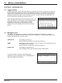
The EZECAL 5 is a general purpose tool intended for the calibration of control equipment, instrumentation
and transducers. It can both simulate and measure simultaneously and is also equipped with a power supply
output to provide loop power for 2 wire transmitters.
The EZECAL 5 is a high precision instrument, and as such must be recalibrated regularly ( at least once per
year ) to maintain optimum performance. For the users convenience, the date of the last calibration is shown
on the display every time the unit is switched on.
The integral high capacity battery pack makes the instrument suitable for both field use (providing up to 10 hours continuous operation
from one charge), and laboratory work using the mains power supply adapter.
In the field the EZECAL 5 can store around 200 calibration measurements or log 400 values for later retrieval
back at the office, where the optional RS232 interface may be use to print calibration certificates or dump
logged data into a PC spreadsheet for analysis.
1.1
Display and Keyboard.
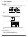
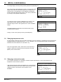
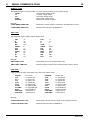
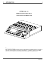
When first switched on, the display shows the instrument serial number and the date of the last calibration.
FGH
EZECAL Mk5 V1.00
SERIAL NO. 12345
LAST CAL: 16 JUN 03
Fig 2
After 5 seconds this display is replaced by the primary working screen.
BATTERY CONDITION
MESSAGE LINE
RECALL ?
OUTPUT ICON
1234.5
TC:K
INPUT ICON
SIMULATED VALUE
mV
CJC:MAN
mV
1234.5
TC:K
CJC:MAN
RANGE MODE CONF LOOP
SIMULATE RANGE
MEASURED VALUE
MEASUREMENT
RANGE
FUNCTION KEY LABELS
Fig 3
M35 Issue 1
2
EZECAL 5 USER MANUAL
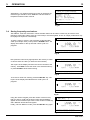
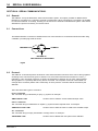
The primary display of the calibrator is divided into four main areas.
MESSAGE LINE
Shows prompt messages for the STORE and RECALL facilities.
FUNCTION KEY LABELS
The purpose of the four function buttons F1 to F4 change depending upon the screen mode. The function
key labels tell the operator the purpose of the buttons for the current screen. For example, in the above
illustration F1 is used to change the measure or simulate range.
BATTERY CONDITION INDICATOR
This symbol shows the charge status of the battery pack. It is animated in six stages from fully charged
(completely black) to low charge (all white) and critically low (all white and flashing).
Fig 2
STORE
REPLAY
48.83
mV
TC:K
LOG
RECALL
1200.0
°C
CJC:MAN
100mV
RANGE MODE CONF LOOP
F1
F2
F3
F4
7
8
9
4
5
6
1
2
3
+/-
0
Fig 4
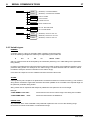
The keyboard is split into three areas:-
NUMERIC KEYPAD
The numeric keypad is used to enter numeric data in exactly the same way as a calculator.
Numbers are entered in exactly as written followed by the ENTER key. The decimal point position is taken
care of automatically depending on the circumstances. Mistakes can be rectified simply by re-entering the
correct value and pressing ENTER.
M35 Issue 1
1:
INTRODUCTION
3
CONTROL WHEEL
Alternatively, any number which can be entered via the numeric keypad, may be entered by
turning the 'control wheel'. Turning the knob clockwise increases the displayed number and
anticlockwise decreases the number. The rate at which the displayed number changes is
dependent on the speed at which the pot is turned, so spinning the knob quickly will change
the displayed number at several hundred digits per second.
The sensitivity of the control wheel is adjusted dynamically by the EZECAL 5 to suit the type
of value actually being changed and the overall sensitivity (speed of response) may be
adjusted as desired from the configuration menu (see 5.3).
Fig 5
FUNCTION KEYS
These four keys are used to select functions dependent upon the screen currently shown. Their function is
indicated at all times by the function key labels on the bottom line of the display.
FEATURE KEYS
These four keys provide access from the primary display to the STORE, RECALL, LOG and REPLAY
features described in later sections.
1.2
Batteries.
The EZECAL 5 has a fixed internal NiCad battery pack. This battery pack is inaccessible to the user and
cannot be replaced by dry cells.
The useful life of the batteries depends on the use of calibrator. To obtain the longest use from one charge,
the user should observe the following guidelines.
•
•
•
Switch off the calibrator when not in use.
Use the backlight only when necessary.
Use the 24V transmitter supply only when power is unavailable elsewhere.
The internal battery pack must be recharged using the power supply adaptor provided. To charge the
batteries simply plug the adaptor power lead into the power jack at the rear of the instrument.
With the instrument switched off, recharging will take approximately 14 hours. Do not charge for significantly
longer than this as damage may be caused to the batteries.
The instrument may be used whilst the battery is recharging, however the charge rate will be reduced and
the recharge time will be significantly lengthened.
For optimum battery performance, the batteries should be run down to their minimum operating level before
recharging.
M35 Issue 1
4
EZECAL 5 USER MANUAL
SECTION 2 - CONNECTIONS.
2.0
Terminals.
On the top of the EZECAL 5 are two rows of terminals. Each terminal can accept a 4mm banana type plug,
or be used to clamp the bare end of a wire. The terminal function is indicated on the label and in the figure
below.
Fig 6
2.1
Voltage Measurement.
The unit under test is connected directly to the COM and V+ terminals shown.
For low level voltage measurements on the 100mV range see section 2.10 for hints on accuracy.
Fig 7
2.2
Current Measurement.
Devices which can source current ( such as controller outputs and mains powered transmitters ) may be
measured by connecting them to the I+ and COM- input terminals.
M35 Issue 1
2:
CONNECTIONS
5
DEVICE
UNDER
TEST
I+
Fig.8
Other devices such as loop powered transmitters, are only capable of sinking current and hence require a
power supply in order to work. For this type of device the integral power supply should be wired in series with
the current loop.
DEVICE
UNDER
TEST
I+
24V+
24V-
Fig.9
2.3
Resistance / RTD Measurement.
The resistor or resistance thermometer to be measured should be connected in 3 wire mode as shown. For
the highest precision, the 3 wires used should be of the same gauge and length. This allows the
measurement to compensate for the resistance of the lead wires.
A two wire measurement may be made by shorting together terminals R2 and R3 and connecting the resistor
to be measured between terminals R1 and R2. In this case however the displayed resistance will include the
resistance of the lead wires.
M35 Issue 1
6
EZECAL 5 USER MANUAL
Fig.10
2.4
Thermocouple Measurement.
There are two modes of thermocouple measurement available depending on the location of the reference
junction.
For thermocouples wired in compensating cable, the cables should be directly connected to the voltage
measurement terminals and the EZECAL 5 should be set to REF:INTERNAL. For best results, the
compensating wire tails should be bare wire and should be tightly clamped under the terminals.
Fig.11
Alternatively an external reference junction may be used. In this case the cables from the reference junction
should be connected as shown and the EZECAL 5 set to REF:MANUAL with the reference temperature Tref
manually entered.
M35 Issue 1
2:
CONNECTIONS
7
Fig 12
2.5
Voltage Simulation.
Connect up the unit under test to the V- and V+ terminals as shown. For simulation on the 100mV range, pay
particular attention to the guidelines given in section 2.10.
Fig 13
2.6
Current Simulation.
The current output terminals I- and I+ do not source current and so the internal 24V power supply should be
connected in series as shown to provide loop power. An existing supply may be used (as in a two wire
transmitter loop). In this case connection need only to be made to the I- and I+ terminals.
M35 Issue 1
8
EZECAL 5 USER MANUAL
Fig 14
2.7
Resistance/RTD Simulation.
For the most accurate resistance simulation the unit under test should be connected using the four wire
method shown below. This method cancels out the resistance of the wiring. Pay particular attention to the
polarity of the measurement current sourced from the unit under test.
NOTE.
When calibrating instruments with scanning inputs (such as chart recorders), the scanning should be turned
off such that the instrument under test is constantly measuring the input to which the EZECAL 5 is
connected.
Fig 15
If the unit under test employs a three wire measurement technique, then connect the wires as shown below.
M35 Issue 1
2:
CONNECTIONS
9
Fig 16
2.8
Thermocouple Simulation.
There are two modes of thermocouple simulation available depending on the location of the reference
junction.
For connection in compensating cable to the unit under test, the cables should be directly connected to the
voltage simulation terminals and the EZECAL 5 should be set to REF:INTERNAL. For best results, the
compensating wire tails should be bare wire and should be tightly clamped under the terminals.
Fig 17
Alternatively an external reference junction may be used. In this case the cables from the reference junction
should be connected as shown below and the EZECAL 5 set to REF:MANUAL with the reference
temperature Tref manually entered.
M35 Issue 1
10
EZECAL 5 USER MANUAL
Fig 18
2.9
Transmitter power supply.
A 24V dc power supply is available to power two wire transmitters or any other current input/output device.
The power supply is current limited to a nominal 25mA.
2.10 Hints for accurate low level voltage measurement and simulation.
When measuring or simulating low voltage levels such as thermocouple signals, the user can unwittingly
introduce errors into the measurement. These errors are usually due to thermal emfs. Thermal emfs are
small voltages which appear across joints of dissimilar metals. If two or more such joints are at differing
temperatures then the resultant voltage will be added to the measurement/simulation voltage. Best results
will be obtained by following the simple guidelines given below.
Always use the correct type of compensating cable for thermocouples that require it and pay particular
attention to the polarity (red is not always positive). Some thermocouples (notably type B) do not require
compensating cable.
When compensating leads are to be connected directly to the EZECAL 5, the bare wire ends should be
firmly clamped under the terminals to allow the EZECAL 5 to make an accurate reference junction
temperature measurement.
Avoid the use of banana plugs if possible, but if they are to be used, then handle them lightly by the plastic
part to avoid warming them up.
Wait for several minutes after wiring to allow time for the temperature of the connections to equalise before
making the measurement. This will reduce any thermal emf effects which do occur.
M35 Issue 1
3:
OPERATION
11
SECTION 3 - OPERATION.
3.0
Operating mode.
The EZECAL 5 has three primary operating modes. To change the mode, simply press F2 (MODE).
MEASURE ONLY MODE.
48.83 mV
In this mode the display shows only the measured input.
Although the simulated output is still functioning.
100mV
RANGE MODE CONF
Fig 19
SIMULATE ONLY MODE.
1200.0
In this mode the display shows only the simulate output value.
To change the simulate output, enter the new value via the
numeric keypad or rotate the control wheel as required.
TC:K
°C
CJC:MAN
RANGE MODE CONF
Fig 20
SIMULATE/MEASURE MODE.
1200.0
In this mode both the simulated output and the measured
inputs are shown. As in simulate only mode the simulated
output may be entered at any time.
TC:K
°C
CJC:MAN
mV
48.83
100mV
RANGE MODE CONF LOOP
Fig 21
If F4 (LOOP) is pressed, then the simulate output value is
forced to numerically equal the measured input value. This fact
is indicated by the line now drawn between the input and the
output icons.
This mode is useful when the ezecal is used as a conversion
tool (eg to convert signals between different thermocouple
types).
1200.0
TC:K
°C
CJC:MAN
mV
48.83
100mV
RANGE MODE CONF LOOP
Fig 22
To exit from loop mode, simply press F4 (LOOP) again.
3.1
Changing range.
The EZECAL 5 is equipped with 20 standard ranges plus four user defined ranges. The range must be
selected for both the simulation output and the measurement input and hence there is a range select screen
for each.
M35 Issue 1
12
EZECAL 5 USER MANUAL
To change range, from the primary screen press the F1 (RANGE) key.
The current range name selected is shown on the top line of the
display along with the associated range units, resolution and
reference type. The parameter to be modified is indicated by
means of the triangular pointer (cursor). This can be positioned
by pressing the F1 (DOWN ARROW) key.
SIMULATION RANGE
RANGE:>TC:K
UNITS: 0.1°C
REF
: INTERNAL
VALUE: 25.3°C
|
NEXT MEAS QUIT
Fig.23
Fig 23
To change the range, press the F2 (NEXT) key and the next
range will be shown. Alternatively rotate the pot until the
required range is shown. See appendix A for a list of available
ranges.
To toggle between the simulation and measurement range
screens press the F3 key.
MEASUREMENT RANGE
RANGE:>100mV
UNITS: 0.01mV
REF
: N/A
VALUE: N/A
|
NEXT SIM
QUIT
Fig 24
Finally, to return to the primary screen press F4 (QUIT).
3.2
Changing temperature units.
On temperature ranges the user can select the display units and resolution. Temperatures may be displayed
in degrees Celsius or Fahrenheit and in 1° or 0.1° resolution. On non temperature ranges, the UNITS line
indicates units and resolution for information only.
SIMULATION RANGE
From the range select screen, index down to the UNITS line
using F1. Select the required units and resolution using F2
(NEXT) or the control wheel.
RANGE: TC:K
UNITS:>0.1°F
REF
: INTERNAL
VALUE: 77.5°F
|
NEXT MEAS QUIT
Fig 25
3.3
Changing cold junction mode.
For accurate measurement or simulation of thermocouples the EZECAL 5 must compensate for the
temperature of the reference junction.
SIMULATION RANGE
If the thermocouple is wired to the EZECAL 5 in compensating
cable then this reference junction exists at the terminals of the
calibrator and the cold junction mode should be set to
INTERNAL.
RANGE: TC:K
UNITS: 0.1°F
REF
:>INTERNAL
VALUE: 77.5°F
|
Fig 26
M35 Issue 1
NEXT MEAS QUIT
3:
OPERATION
13
SIMULATION RANGE
Alternatively, if an external reference junction is used then the
reference type should be set to MANUAL and the reference
temperature entered under VALUE.
RANGE: TC:K
UNITS: 0.1°F
REF
: INTERNAL
VALUE:>77.5°F
|
NEXT MEAS QUIT
Fig 27
3.4
Saving frequently used values.
The EZECAL 5 has ten memories in which simulate values can be stored. These may be used to store
frequently used output values (such as 0 and 1000) or be used together to form an output profile which may
be replayed in sequence automatically.
To store a value in memory, first of all enter a valid simulate
value (for example 100.0). Then press the STORE button. The
display will indicate on the top line that a store cycle is in
progress.
STORE
?
100.0
TC:K
°C
CJC:MAN
RANGE MODE CONF
Fig 28
Now press the numeric key appropriate to the memory in which
ou wish to store the value (or rotate the control wheel).
STORE 1 (
10.0)
100.0
The top line of the display will show the current contents of the
memory. Press ENT to store the value in the selected memory
or press STORE to abort without saving.
TC:K
°C
CJC:MAN
RANGE MODE CONF
Fig 29
To recover a value from memory press the RECALL key. The
top line of the display will indicate that a recall cycle is in
progress.
RECALL ?
100.0
TC:K
°C
CJC:MAN
RANGE MODE CONF
Fig 30
Using the numeric keypad, press the number of the memory
that you wish to recall and the stored value will immediately
appear as the simulate output value. Press another number key
and a different stored value will appear.
Finally, exit from RECALL mode, press the RECALL key again.
RECALL
2
200.0
TC:K
°C
CJC:MAN
RANGE MODE CONF
Fig 31
M35 Issue 1
14
EZECAL 5 USER MANUAL
SECTION 4 - ADVANCED FEATURES.
4.0
Logging.
The EZECAL 5 logger can operate in one of two modes.
MEASUREMENT v TIME
The logger will log the value of the measured input at fixed time intervals.
CALIBRATION POINTS
The logger will store calibration data files.
The logger function is set up under the configuration menu see 5.1.
4.1
Measurement versus time logging.
In this mode the logger will record the value of the measured input at preset time intervals. 400 such logs
can be made and the data obtained can be replayed in graphical form, output from the simulate output or
down loaded via the serial communications option into a personal computer for later analysis. Once started
the logging continues to operate in the background until 400 logs have been made or is manually stopped.
While the logger is running the calibrator may continue to be used in the normal way.
Before the logger can be started, the log interval must be entered. From the primary display press the LOG
key and the logger control display will appear.
The STATUS line shows the current logger status, either
STOPPED or RUNNING. The next line shows the programmed
log interval in minutes and seconds, in this case 1 minute is set.
LOGGER
STATUS
:STOPPED
LOG EVERY
: 1:00
CURRENT LOG:
NEXT LOG IN :
START STOP
QUIT
Fig. 32
This value may be set as required using the numeric keypad or
the control wheel between one second and ten minutes.
LOGGER
STATUS
:STOPPED
LOG EVERY
: 0:30
CURRENT LOG:
NEXT LOG IN :
START STOP
QUIT
Fig. 33
The logger can now be started by pressing F1 (START). The
display will now show two additional pieces of information. The
number of logs made and the time remaining before the next
log is made. Use F2 (STOP) to stop the logger if required.
LOGGER
STATUS
:RUNNING
LOG EVERY
: 0:30
CURRENT LOG:
1
NEXT LOG IN : 0:23
START STOP
Fig. 34
M35 Issue 1
QUIT
4:
ADVANCED FEATURES
15
To return to the primary screen press the F4 (QUIT) key. The
primary display will now indicate that the logger is running by
showing a small LG symbol underneath the measure icon.
1200.0
TC:K
°C
CJC:MAN
mV
48.83
LG
100mV
RANGE MODE CONF LOOP
Fig.35
4.2
Retrieving logged data.
Logged data may be retrieved in one of three ways. It may be shown on the display as a graph. It may be
replayed in real time from the simulate output or may be down loaded to a personal computer via the serial
communications option.
The replay option required is selected by pressing REPLAY from the primary screen.
4.2.1 Display log graph.
From the replay options screen move the cursor to SHOW
LOG GRAPH using the F1 key and press F2 (SELect) to select
the log graph display.
REPLAY
>
SHOW LOG GRAPH
<
REPLAY LOGGED
REPLAY STORED
DUMP LOG VALUES
|
SEL
QUIT
Fig.36
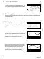
The graph y axis is automatically scaled to accommodate the
range of the logged values and the first one hundred logs are
shown across the display. If the logger is actually running while
the graph is shown, then the graph will automatically be
updated with any new values as they are logged.
0:00:00:00 50.23mV
IN OUT CENT
QUIT
Fig.37
A vertical cursor line is provided in order to read off the time
and value at the point where the cursor intersects the graph.
The cursor is positioned using the control wheel and the
associated elapsed time in days, hours, minutes and seconds
is shown below the graph along with the actual input value at
that time. If the cursor is moved to the far right of the graph
then the next page of logged points will be displayed.
0:00:00:00 50.23mV
IN OUT CENT
QUIT
Fig.38
M35 Issue 1
16
EZECAL 5 USER MANUAL
To show more detail, the user may zoom in on the graph using
F1 (IN). This will cause the y axis to expanded by a factor of 2
and the graph to be centred on the currently selected (flashing)
point. Repeated presses of F1 will cause greater magnification
up to the maximum limit of ten digits on the y axis. To zoom out
again use F2 (OUT), or to centre the flashing point use F3
(CENT).
0:00:00:00 50.23mV
IN OUT CENT
QUIT
Fig. 39
To exit from the graph display and return to the replay options screen press F4 (QUIT).
4.2.2 Replay logged data.
The data recorded by the logger can be replayed via the simulate output. Once started the replay will
continue automatically at the programmed rate until all of the logged points have been replayed or the replay
is manually stopped.
From the replay options screen, move the cursor to REPLAY
LOGGED using F1 and select using F2 (SELect). The replay
control screen will appear.
REPLAY
>
SHOW LOG GRAPH
REPLAY LOGGED
<
REPLAY STORED
DUMP LOG VALUES
|
SEL
QUIT
Fig. 40
The STATUS line shows the current replay status, either
STOPPED or RUNNING. The next line shows the programmed
replay interval in minutes and seconds, in this case 1 minute is
set.
The replay interval may be set as required between 1 second
and 10 minutes per step using the numeric keypad or control
wheel.
REPLAY LOGGED
STATUS
:STOPPED
REPLAY EVERY : 1:00
REPLAY MODE : STEP
CURRENT STEP :
NEXT STEP IN :
START STOP MODE QUIT
Fig.41
The replay mode may be toggled between STEP and RAMP
using F3 (MODE). In STEP mode the calibrator will step
change the simulate output between the logged data values. In
RAMP mode the calibrator will ramp the simulate output by
interpolating between the logged points every one second. This
option may be changed while the replay is running.
REPLAY LOGGED
STATUS
:STOPPED
REPLAY EVERY: 1:00
REPLAY MODE : RAMP
CURRENT STEP:
NEXT STEP IN:
START STOP MODE QUIT
Fig 42
M35 Issue 1
4:
ADVANCED FEATURES
The replay may be started using F1 (START) or stopped by
using F2 (STOP). While the replay is running both the current
step number and the time remaining until the next step is
shown on the display.
17
REPLAY LOGGED
STATUS
:RUNNING
REPLAY EVERY: 1:00
REPLAY MODE : RAMP
CURRENT STEP:
5
NEXT STEP IN: 0:37
START STOP MODE QUIT
Fig 43
To return to the primary screen press the F4 (QUIT) key. The
primary display will now indicate that the replay is running by
showing a small RP symbol underneath the simulate icon.
While this is present the simulate output value may not be
changed manually.
RP
1200.0
TC:K
°C
CJC:MAN
mV
48.83
100mV
RANGE MODE CONF LOOP
Fig 44
4.2.3 Replay stored data.
This option is identical to the REPLAY LOGGED option except that the values replayed will be the ten values
saved in memory using the STORE key. Linking the ten STORED values in this manner enables the user to
create a 'test profile'. Unlike the REPLAY LOGGED option, the test profile will be repeated over and over
until the replay is manually stopped.
This 'test profile' can be useful, for example when checking the calibration of an instrument mounted in a
control panel. In this case the calibrator would be connected inside the panel to the instrument and the test
profile entered as described in 3.4. The EZECAL 5 would then be set to replay the stored profile at say 1
minute per step. The operator need now only to observe the instrument readings from the front of the panel
and record them if necessary.
4.2.4 Dump log values.
Data collected by the logger may be down loaded to a computer for analysis or printing. This is only available
if the serial communications option is fitted. The data is transmitted using standard ASCII characters in a
format suitable for most popular spreadsheet programmes.
From the replay options screen, move the cursor to DUMP
LOG VALUES using F1 and select using F2 (SELect).
REPLAY
SHOW LOG GRAPH
REPLAY LOGGED
REPLAY STORED
> DUMP LOG VALUES
|
SEL
<
QUIT
Fig 45
M35 Issue 1
18
EZECAL 5 USER MANUAL
DUMP LOG VALUES
The log dump confirmation screen will now appear. Ensure that
the computer to be used is both connected and ready to receive
data, then press F3 to transmit the data.
DUMP DATA NOW ?
ARE YOU SURE ?
YES
QUIT
Fig 46
While the data is being transmitted the display will show the
word DUMPING. This may take some time for slow baud rates
and large amounts of logged data. When complete the replay
options menu will re appear.
DUMP LOG VALUES
DUMP DATA NOW ?
ARE YOU SURE ?
DUMPING...
YES
QUIT
Fig 47
4.2
Storing calibration records.
The alternative use for the logger is to store calibration records. This mode of operation is set up from the
configuration menu under LOGGER FUNCTION see 5.1.
A calibration record is a file stored within the calibrator which records the before and after calibration
performance of an instrument or transmitter. The EZECAL 5 can store many such files depending on the
number of calibration points used within each file.
Once a calibration file is stored, it can be examined, dumped to a computer or printed out as a calibration
certificate on a suitable serial printer.
This powerful feature allows many instruments to be calibrated during a day in the field and the results
stored within the calibrator. Then, upon return to the office or car, the calibration certificates printed out and
signed.
A typical calibration sequence would consist of the following steps:-
1.
Set up the simulate output and measure input to suit the unit under test.
For display only devices (such as a panel meter), set the EZECAL to simulate only mode.
2.
For devices which have a measurable output (such as a transmitter), set the EZECAL to
simulate/measure mode.
Open a new calibration record file.
3.
Record the uncalibrated performance of the unit under test at several points within its range.
4.
Close the calibration record file.
5.
Calibrate the unit under test.
6.
Record the calibrated performance of the unit under test.
M35 Issue 1
4:
ADVANCED FEATURES
7.
Repeat steps 1 to 6 on other units.
8.
Print out and sign calibration certificates.
19
4.2.1 Opening a calibration record file.
Before any records can be stored, the calibration file must be opened. This merely consists of giving the file
a name. The file name is a string of up to seven characters and would normally be the tag name or serial
number of the instrument to be calibrated. File names need not be unique, but in this case it is up to the user
to distinguish between identically named files. Files are stored in memory and each file occupies 24 bytes
plus 6 bytes per record.
From the primary display press the LOG key and the cal' record
menu screen will appear. The amount of free memory is
displayed in bytes at the bottom of the screen. Point to OPEN
NEW FILE using F1 and press F2 to select.
CALIBRATION RECORD
> OPEN NEW FILE
POST CAL RECORDS
<
868 BYTES MEM FREE
|
SEL
QUIT
Fig 48
The EZECAL 5 will invite you to enter the name of the new file.
Initially the file name will be set to 'UNNAMED' and this may be
overwritten as required. The file name is entered one character
at a time using the numeric keys, control wheel or F2 (NEXT).
All alphanumeric characters and punctuation may be used in
the file name. The character being entered is indicated by the
flashing underline cursor. When the correct character is
displayed, press the ENTER key to advance to the next
character position or F3 (CLeaR) to blank the character. When
complete press F1 (OPEN) to open the file or F4 (QUIT) to
abort.
If the file is opened the user may then enter the tag name or
serial number of the device being calibrated. This is done in the
same manner as the file name. Press F1 (DONE) when
complete or F4 (QUIT) to abort.
OPEN NEW CAL FILE
FILE NAME : UNNAMED
TAG NAME :
OPEN
NEXT
CLR
QUIT
Fig 49
OPEN NEW CAL FILE
FILE NAME : UNNAMED
TAG NAME :
OPEN NEXT CLR QUIT
Fig 50
The primary display will show the LG symbol to indicate that a calibration file is open and that the EZECAL 5
is now ready to store the pre calibration values.
4.2.2 Saving a pre calibration point.
After setting the simulate output to the required pre calibration point on the primary display, press the LOG
key. The PRE CAL RECORD screen will appear.
M35 Issue 1
20
EZECAL 5 USER MANUAL
The current simulate output value is displayed as the INPUT
value on the display (because it is the input to the unit under
test). If the unit under test has a measurable output, then this
output value is displayed as the PRE CAL value. Alternatively
for display only devices, the PRE CAL value is displayed as
zero and the engineer should enter the current display reading
of the unit under test. In either case the values should be saved
by pressing F3 (SAVE) at which point the screen will revert to
the primary display.
PRE CAL RECORDS
FILE
: TIC 112
REC No : 0
INPUT
: 100.0°C
PRE CAL :
4.09mV
FREE MEM: 140 RECS
CLOSE
SAVE QUIT
Fig 51
The bottom line on the display shows the available memory
space in records. Up to forty such records can be entered into one calibration file.
4.2.3 Closing the pre calibration record file.
When all necessary calibration points have been recorded, the calibration file should be closed to save away
all the pre calibration data.
Once the file is closed it may not be re-opened and the pre calibration points may not be edited.
From the primary display press the LOG key to access the pre
calibration record screen. The display will show the number of
records which have been saved.
Press F1 (CLOSE) to close the file or F4 (QUIT) to return to
the primary display.
PRE CAL RECORDS
FILE
: TIC 112
REC No : 17
INPUT
: 100.0°C
PRE CAL :
4.09mV
FREE MEM: 123 RECS
CLOSE
SAVE QUIT
Fig 52
4.2.4 Recording post calibration data.
Once the unit under test has been calibrated, the calibrated performance should be recorded.
CALIBRATION RECORD
From the primary display, press the LOG key and point to
'POST CAL RECORDS' using F1 and select using F2
(SELect).
OPEN NEW FILE
> POST CAL RECORDS <
|
SEL
QUIT
Fig 53
SELECT FILE
Point to the required file from the menu by using F1 and then
press F2 (SELect) to select the indicated file. If more than six
files are stored then press F3 (MORE) to display the next
page.
>
TIC 112
TIC 110
LI 224
2467812
17
12
09
10
<
|
MORE
QUIT
Fig 54
M35 Issue 1
SEL
4:
ADVANCED FEATURES
21
When the file has been selected the post calibration record screen will appear. The EZECAL 5 will
automatically set the simulate and measure ranges to those set at the time when the pre cal records were
stored and the simulate output will be set to source the INPUT value shown.
For devices with a measurable output, the POST CAL value will
show the current output from the unit under test. When this
value has settled, press the F3 (SAVE) key to store the post
calibration value for that calibration point.
POST CAL RECORDS
FILE
: TIC 112
REC No : 1
INPUT
: 100.0°C
PRE CAL :
4.09mV
POST CAL:
4.10mV
NEXT PREV SAVE QUIT
Fig 55
For display only devices the POST CAL value will appear blank
and the value displayed on the unit under test should be
entered manually using the keypad or control wheel. Press F3
(SAVE) to store the value in memory. POST CAL values which
have been saved are indicated by a star appearing before the
displayed value.
Press F1 (NEXT) to advance to the next calibration point. Again
the EZECAL 5 will automatically set the simulate output to the
correct value ready for the operator to enter or save the post
calibration reading as before.
POST CAL RECORDS
FILE
: TIC 112
REC No : 1
INPUT : 100.0°C
PRE CAL : 4.09mV
POST CAL:* 4.10mV
NEXT PREV SAVE QUIT
Fig 56
Continue using F1 (NEXT) or F2 (PREVious) until all post calibration points have been done. Press F4
(QUIT) to return to the primary display.
4.3
Retrieving calibration records.
There are three ways in which stored calibration files can be retrieved.
1.
2.
3.
The calibration data can be shown one point at a time on the EZECAL 5 display.
The calibration data can be down loaded to a personal computer via the serial communications option
if fitted.
The EZECAL 5 can be connected to a suitable serial printer and a calibration certificate can be printed
out.
To perform any of these three options, from the primary display press the REPLAY key and the CAL
RECORD REPLAY screen will appear.
CAL RECORD REPLAY
Select the option required using F1 to move the cursor and F2
(SELect) to select the indicated option.
> SHOW CAL FILE
<
DELETE CAL FILE
PRINT CAL CERT
DUMP CAL DATA
|
SEL
QUIT
Fig 57
M35 Issue 1
22
EZECAL 5 USER MANUAL
4.3.1 Show calibration file.
When this option is selected the file selector menu will appear.
The file selector shows all the files currently stored within the
calibrator in the order that they were created. The number of
records contained within the file is shown next to the file name.
To select the file of interest, move the triangular pointer with the
F1 key and press F2 (SELect) to select the indicated file. If the
file required is not shown on the display then press F3 (MORE)
to show the next page of files.
SELECT FILE
>
TIC 112
TIC 110
LI 224
2467812
|
SEL
17
12
09
10
<
MORE
QUIT
Fig 58
CALIBRATION RECORD
The calibration records are shown one point at a time. The user
can scan through the records by pressing F1 (NEXT) to show
the next point, or F2 (PREVious) to show the previous point.
The record number shown will end around to 1 at the end of the
list. If the POST CAL value is shown blank then the post cal
figure was not saved for that calibration point. Press F4 (QUIT)
to return to the cal record replay screen.
FILE
: TIC 112
REC No : 1
INPUT
: 100.0°C
PRE CAL :
4.09mV
POST CAL:
4.10mV
NEXT
PREV
QUIT
Fig 59
4.3.2 Print calibration certificate.
When this option is selected the file selector menu will appear.
The file selector shows all the files currently stored within the
calibrator in the order that they were created. The number of
records contained within the file is shown next to the file name.
To select the file of interest, move the triangular pointer with the
F1 key and press F2 (SELect) to select the indicated file. If the
file required is not shown on the display then press F3 (MORE)
to show the next page of files.
SELECT FILE
>
TIC 112
TIC 110
LI 224
2467812
|
SEL
17
12
09
10
<
MORE
QUIT
Fig 60
PRINT CAL RECORD
Ensure that the printer is connected, on line and that the paper
is correctly aligned. Finally press F3 (YES) if everything is
ready for printing or F4 (QUIT) to abort.
PRINT FILE TIC 112
ARE YOU SURE ?
YES
QUIT
Fig 61
PRINT CAL RECORD
The print screen will remain until the print out has finished.
PRINT FILE TIC 112
ARE YOU SURE ?
PRINTING...
YES
Fig 62
M35 Issue 1
QUIT
4:
ADVANCED FEATURES
23
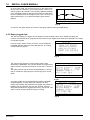
An example of a typical calibration certificate is shown below. All that now needs to be done is to sign and
date it.
CALIBRATION CERTIFICATE
TEST EQUIPMENT.
FGH EZECAL Mk5 SERIAL
EZECAL S/W VERSION
LAST CAL. DATE
CALIBRATION FILE
DEVICE UNDER TEST
:
:
:
:
:
11111
V1.00
05/10/93
TIC 112
1865241
TEST RESULTS
INPUT
degC
0.0
250.0
500.0
750.0
1000.0
OUTPUT/READING
PRE CAL
POST CAL
degC
degC
-0.1
250.1
499.8
749.9
999.8
0.0
250.0
500.0
750.1
1000.1
SIGNED
DATE
4.3.3 Dump calibration data.
The calibration data may be down loaded to a personal computer if the serial communications option is fitted.
The data is transmitted in serial form using ASCII characters only and is in a format suitable for most popular
spreadsheet programmes.
When this option is selected the file selector menu will appear.
The file selector shows all the files currently stored within the
calibrator in the order that they were created. The number of
records contained within the file is shown next to the file name.
To select the file of interest, move the triangular pointer with the
F1 key and press F2 (SELect) to select the indicated file. If the
file required is not shown on the display then press F3 (MORE)
to show the next page of files.
SELECT FILE
>
TIC 112
TIC 110
LI 224
2467812
|
SEL
17
12
09
10
<
MORE
QUIT
Fig 63
Ensure that the computer is connected and ready to receive
data. Finally press F3 (YES) if everything is ready and the
calibration point data will be transmitted to the computer or
press F4 (QUIT) to abort.
DUMP CAL RECORD
DUMP FILE TIC 112
ARE YOU SURE ?
YES
QUIT
Fig 64
M35 Issue 1
24
EZECAL 5 USER MANUAL
This display will remain until the file has been transmitted. At
which point the screen will return to the file selector menu in
order that another file may be down loaded if required.
DUMP CAL RECORD
DUMP FILE TIC 112
ARE YOU SURE ?
SENDING...
YES
QUIT
Fig 65
4.4
Deleting a calibration file.
After the calibration file has been printed or down loaded as necessary the calibration file may be deleted
from memory.
CAL RECORD REPLAY
From the cal record replay menu, select the delete file option
using F1 to move the cursor and F2 (SELect) to select.
SHOW CAL FILE
> DELETE CAL FILE <
PRINT CAL CERT
DUMP CAL DATA
|
SEL
QUIT
Fig 66
Select the file name to be deleted from the file selector menu
and press F2 (SELect) to select the chosen file. If the file
required is not shown on the display then press F3 (MORE) to
show the next page of files.
SELECT FILE
>
TIC 112
TIC 110
LI 224
2467812
|
SEL
17
12
09
10
<
MORE
QUIT
Fig 67
DELETE CAL RECORD
On the confirmation screen press F3 (YES) if you are certain
that you want to delete the chosen file. Remember calibration
files cannot be recovered once they have been deleted.
DELETE FILE TIC 112
ARE YOU SURE ?
YES
QUIT
Fig 68
4.5
Custom ranges.
The EZECAL 5 is capable of storing up to four user defined ranges known as custom ranges. These are
used when a standard EZECAL range is not appropriate for the specific non standard simulation or
measurement required.
Once a custom range is defined it remains resident within the calibrator ready to be called up by name the
next occasion it is needed. The same custom range may be used for both input and output ranges,
depending on whether it is called up as a simulation or measurement range.
M35 Issue 1
4:
ADVANCED FEATURES
25
Example of a custom range.
Consider a head mounted thermocouple transmitter which accepts as its input a type K thermocouple, and
outputs a non linearised 4-20mA signal over the range 200°C to 800°C
Checking the calibration of such a transmitter over its range would normally involve a lot of tedious
calculations using look up tables.
EZECAL 5 makes this task simple by the use of a custom range.
Programming the range.
Custom ranges are defined under the CUSTOM RANGE option on the configuration menu. To illustrate the
setting up procedure we take the above thermocouple transmitter as our example.
From the primary display, press F3 (CONFigure) and then
select CUSTOM RANGES.
CONFIGURATION MODE
> CUSTOM RANGE
<
CUSTOM LAW
LOGGER FUNCTION
BACKLIGHT CONTROL
POT SENSITIVITY
COMMUNICATIONS
|
SEL
QUIT
Fig 69
Select a spare range number or pick an existing range to be
overwritten using F2 (NEXT) or the control wheel.
CUSTOM RANGE SETUP
NUMBER:> 1
NAME : CUSTOM1
RANGE : 100mV
LAW
: LINEAR
UNITS : mV
RES
: 0.01
| NEXT LIMS QUIT
Fig 70
Press F1 (DOWN ARROW) to advance down to the range
name. Enter the required name for the range. The name is
entered one character at a time. The current character is
indicated by the flashing underline cursor and may be moved
by pressing the ENTER key. To change the character above
the cursor, use the numeric keypad or spin the control wheel.
CUSTOM RANGE SETUP
NUMBER: 1
NAME
:> K 4TO20
RANGE : 100mV
LAW
: LINEAR
UNITS : mV
RES
: 0.01
|
NEXT LIMS QUIT
Fig 71
Use F1 again to advance the triangular cursor. Press F2 or spin
the pot to select the range. The range selected is the physical
range required. In our case we require the 20mA range in order
to measure the output from the transmitter.
CUSTOM RANGE SETUP
NUMBER: 1
NAME : K 4TO20
RANGE :> 20mA
LAW
: LINEAR
UNITS : mV
RES
: 0.01
| NEXT LIMS QUIT
Fig 72
M35 Issue 1
26
EZECAL 5 USER MANUAL
Advance down again and enter the law required. In our case the
transmitter output is not linear and follows the type K
thermocouple law. To provide a linear display on the EZECAL 5
we must linearise according to the law 'TC:K'.
CUSTOM RANGE SETUP
NUMBER: 1
NAME
: K 4TO20
RANGE : 20mA
LAW
:> TC:K
UNITS : mV
RES
: 0.01
|
NEXT LIMS QUIT
Fig 73
Advance down again to select the units that we wish on the
EZECAL 5 display using F2 or the control wheel. In our case
we require degrees Celsius.
CUSTOM RANGE SETUP
NUMBER: 1
NAME
: K 4TO20
RANGE : 20mA
LAW
: TC:K
UNITS :> °C
RES
: 0.01
|
NEXT LIMS QUIT
Fig 74
The display resolution parameter merely defines the decimal
point position on the display. It does not increase the resolution
of the calibrator (except on TC or RTD ranges). In our example
we wish to display in tenths degree Celsius. So we set the
display decimal point position to 0.1.
CUSTOM RANGE SETUP
NUMBER: 1
NAME
: K 4TO20
RANGE : 20mA
LAW
: TC:K
UNITS : °C
RES
: > 0.1
|
NEXT LIMS QUIT
Fig 75
Now it is necessary to specify the limits over which the custom range is to work.
Press F3 (LIMS) to enter the custom limit set up screen, and
select again the range number chosen.
CUSTOM LIMIT SETUP
NUMBER :>1
DIS HI : 1000.0°C
DIS LO :
0.0°C
I/O HI : 20.000mA
I/O LO : 0.000mA
T.COMP : N/A
| NEXT RANGE QUIT
Fig 76
Use F1 to point to the DISPLAY HI LIMIT. This is the maximum
number which can appear on the display. In our case this is
800.0°C which corresponds to an input signal of 20mA. For a
simulate range, this number should be the highest allowable
output value which can be set on the display.
CUSTOM LIMIT SETUP
NUMBER : 1
DIS HI :> 800.0°C
DIS LO :
0.0°C
I/O HI : 20.000mA
I/O LO : 0.000mA
T.COMP : N/A
| NEXT RANGE QUIT
Fig 77
M35 Issue 1
4:
ADVANCED FEATURES
Use F1 again to point to the DISPLAY LO LIMIT. This is the
minimum number which can appear on the display. In our case
this is 200.0°C which corresponds to an input signal of 4mA.
For a simulate range, this number should be the lowest
allowable output value which can be set on the display.
27
CUSTOM LIMIT SETUP
NUMBER : 1
DIS HI : 800.0°C
DIS LO :> 200.0°C
I/O HI : 20.000mA
I/O LO : 0.000mA
T.COMP : N/A
| NEXT RANGE QUIT
Fig 78
Now point to the INPUT/OUTPUT HI LIMIT. This is the
maximum physical input or output value which will appear at
the instruments terminals. In our case this is 20.000mA which
corresponds to the DIS HI value of 800°C. For a simulate
range, this number should be the maximum physical output
value to be sourced.
CUSTOM LIMIT SETUP
NUMBER : 1
DIS HI : 800.0°C
DIS LO : 200.0°C
I/O HI :>20.000mA
I/O LO : 0.000mA
T.COMP : N/A
|
NEXT RANGE QUIT
Fig 79
Now point to the INPUT/OUTPUT LO LIMIT. This is the
minimum physical input or output value which will appear at the
instruments terminals. In our case this is 4.000mA which
corresponds to the DIS LO value of 200°C. For a simulate
range, this number should be the minimum physical output
value to be sourced.
CUSTOM LIMIT SETUP
NUMBER : 1
DIS HI : 800.0°C
DIS LO : 200.0°C
I/O HI : 20.000mA
I/O LO :> 4.000mA
T.COMP : N/A
|
NEXT RANGE QUIT
Fig 80
Next we have the temperature compensation parameter. This is
only applicable to non standard thermocouple inputs or outputs
and should be set to the appropriate cold junction
compensation rate in millivolts per degree Celsius. For example
a type K thermocouple would require a temperature
compensation rate of approximately 0.040 mV/°C.
CUSTOM LIMIT SETUP
NUMBER : 1
DIS HI : 800.0°C
DIS LO : 200.0°C
I/O HI : 20.000mA
I/O LO : 4.000mA
T.COMP : >N/A
| NEXT RANGE QUIT
Fig 81
The custom range configuration is now complete and this new range is now available for selection by name
from the simulate or measure range selection screens.
To complete our example of calibrating the thermocouple transmitter the following steps are required.
Connect the transmitter to the EZECAL 5 as shown below.
M35 Issue 1
28
EZECAL 5 USER MANUAL
Fig 82
Select 'K 4TO20' as the measurement range and 'TC;K' as the simulate range.
Set 200.0°C as the simulate output value and adjust the zero control on the transmitter until the measured
input reads 200.0°C.
Set 800.0°C as the simulate output value and adjust the span control on the transmitter until the measured
input reads 800.0°C.
Check the transmitter output at any mid points required.
4.6
Programming custom laws.
Another powerful feature of the EZECAL 5 is ability to accept custom laws. A custom law defines how the
calibrator is to linearise an input signal or to characterise an output signal. Up to four custom law definitions
can be stored at any one time, and any law may be used in association with any custom range.
A custom law is implemented inside the EZECAL 5 as set of straight line segments which approximate to the
shape of the curve required. Up to 15 such line segments may be used within one law. The junction of two
adjacent line segments is called a 'breakpoint' and these breakpoints may be positioned anywhere in the
range of the instrument.
There are a few important points to consider before attempting to program a custom law.
•
•
The function curve to be programmed must be strictly increasing. ie the output from the lineariser
should increase as the input increases.
The function curve should have no discontinuities and no regions where the curve is perfectly flat.
To allow a custom law to be applied to any input or output range, the law is always programmed as an output
law. For example if an exponential type law is programmed for an output, then this law will automatically be
used in reverse when applied to linearise an input. ie it will perform a natural logarithm type law.
M35 Issue 1
4:
ADVANCED FEATURES
29
Consider the following example.
The user wishes to measure and simulate an Iron-Gold/Chromel cryogenic thermocouple. This is not a
standard thermocouple in the EZECAL 5 and so must be programmed as a custom range with a custom law.
The thermocouple has the following characteristic.
Temp' (Input)
-270°C
-267°C
-265°C
-260°C
-255°C
-250°C
-245°C
-240°C
EMF (Output)
-4.714mV
-4.666mV
-4.634mV
-4.555mV
-4.478mV
-4.402mV
-4.327mV
-4.254mV
Temp (Input)
-235°C
-230°C
-225°C
-220°C
-215°C
-210°C
-205°C
-200°C
EMF (Output)
-4.181mV
-4.111mV
-4.041mV
-3.973mV
-3.906mV
-3.839mV
-3.774mV
-3.709mV
The custom law should therefore convert a linear temperature input to a shaped millivolt output. Further, so
that this law may be applied to any input or output range (for example to measure the output of a two wire
transmitter for this couple), the input and output values must be converted to percentages.
From the table above we take four parameters A, B, C, D.
Where
A is the minimum input value (-270)
B is the maximum input value (-200)
C is the minimum output value (-4.714)
D is the maximum output value (-3.709)
We then calculate for each input value I.
( I-A )
× 100
( B-A )
And for each output value O.
( O-C )
× 100
( D-C )
After calculating each value we get the table below.
Breakpoint
0
1
2
3
4
5
6
7
8
9
10
11
12
13
14
15
Temperature
-270
-267
-265
-260
-255
-250
-245
-240
-235
-230
-225
-220
-215
-210
-205
-200
Input %
0.00
4.29
7.14
14.29
21.42
28.58
35.71
42.86
50.00
57.14
64.29
71.42
78.58
85.71
92.86
100.00
EMF
Output%
-4.714
-4.666
-4.634
-4.555
-4.478
-4.402
-4.327
-4.254
-4.181
-4.111
-4.041
-3.973
-3.906
-3.839
-3.774
-3.709
0.00
4.78
7.96
15.82
23.48
31.04
38.51
45.77
53.03
60.00
66.97
73.73
80.40
87.06
93.53
100.00
The custom law is now ready to load into the EZECAL 5.
M35 Issue 1
30
EZECAL 5 USER MANUAL
From the primary display, press F3 (CONFigure) to access the
configuration menu. Then select CUSTOM LAW.
CONFIGURATION MODE
CUSTOM RANGE
> CUSTOM LAW
<
LOGGER FUNCTION
BACKLIGHT CONTROL
POT SENSITIVITY
COMMUNICATIONS
|
SEL
QUIT
Fig 83
Select the law number required by pressing F3 (LAW). The law
editing screen shows four breakpoints at a time and displays
the input and output values as percentages. The triangular
pointer shows the currently selected parameter. Use F1 to
move the pointer to the next value as required. The default law
table shown contains evenly spaced breakpoints and describes
a perfectly linear relationship between input and output.
Breakpoints 0 and 15 are fixed and cannot be modified.
CUSTOM LAW EDIT
EDIT LAW 1
BP
IN%
OUT%
0 > 0.00
0.00
1
6.67
6.67
2 13.33 13.33
3 16.67 16.67
| PAGE LAW QUIT
Fig 84
To enter the calculated values for the new law, advance to
breakpoint 1 input using F1 and enter the required value on the
numeric key pad or control wheel.
CUSTOM LAW EDIT
EDIT LAW
1
BP
IN%
OUT%
0
0.00
0.00
1 > 4.29
6.67
2
13.33
13.33
3
16.67
16.67
|
PAGE LAW QUIT
Fig 85
Then press F1 again and enter the output value for breakpoint
1.
CUSTOM LAW EDIT
EDIT LAW 1
BP
IN%
OUT%
0
0.00
0.00
1
4.29 > 4.78
2 13.33 13.33
3 16.67 16.67
| PAGE LAW QUIT
Fig 86
Continue in the same way and enter the values for all the
breakpoints. When the pointer reaches the last parameter on
the display, the display will automatically advance to the next
page. Alternatively the display may be manually paged by
pressing F2 (PAGE).
CUSTOM LAW EDIT
EDIT LAW 1
BP
IN%
OUT%
0
0.00
0.00
1
4.29
4.78
2
7.14
7.96
3 14.29 > 15.82
|
PAGE LAW QUIT
Fig 87
M35 Issue 1
4:
ADVANCED FEATURES
Continue to enter the values until all four pages have been
completed.
31
CUSTOM LAW EDIT
EDIT LAW
1
BP
IN%
OUT%
4
21.42
23.48
5
28.58
31.04
6
35.71
38.51
7
42.86 > 45.77
|
PAGE LAW QUIT
Fig 88
If a value is entered in error and this error breaks the custom
law rules as described earlier then an asterisk is shown next to
the value. The asterisk will disappear when the error is
corrected.
Now that the new law has been entered, it may be called up
from the custom range set up screen.
CUSTOM LAW EDIT
EDIT LAW
1
BP
IN%
OUT%
4
21.42
23.48
5 >21.42* 31.04
6
35.71
38.51
7
42.86
45.77
|
PAGE LAW QUIT
Fig 89
The following two screens show how the custom range would be set up to measure or simulate the special
thermocouple in the example.
CUSTOM RANGE SETUP
NUMBER: 1
NAME
: FE/AU
RANGE : 100mV
LAW
: CUSLAW1
UNITS : °C
RES
: 1
|
NEXT LIMS QUIT
CUSTOM LIMIT SETUP
NUMBER : 1
DIS HI : -200°C
DIS LO : -270°C
I/O HI : -3.71mV
I/O LO : -4.71mV
T.COMP : 0.021mV/°C
|
NEXT RANGE QUIT
Fig 90
Fig 91
M35 Issue 1
32
EZECAL 5 USER MANUAL
SECTION 5 - CONFIGURATION.
5.1
Logger function.
As described in earlier sections the logger memory may be used for one of two purposes. To store a log
record of measured input versus time, or to hold calibration record files. The selection of this function is
made from the configuration menu. Because the same internal memory area is used for both functions,
changing the function will result in any stored data being lost. So make sure that any logged data is no
longer required before selecting the alternate function.
Select LOGGER FUNCTION from the configuration menu. The
cursor will indicate the current logger mode. Press F2 (LOG) to
use the log memory for time v input logging. Press F3
(CALibration record) to use the logger memory to store
calibration files. Press F4 (QUIT) to abort without changing
function.
LOGGER FUNCTION
>LOG INPUT v TIME
CALIBRATION RECORD
***WARNING***
DATA WILL BE LOST
IF USE IS CHANGED
LOG
CAL QUIT
Fig 92
5.2
Backlight control.
The EZECAL 5 is equipped with a backlight to illuminate the display under bad lighting conditions.
Unfortunately the backlight can require a lot of power from the batteries. To help increase battery life the
backlight can operate in one of three modes.
ALWAYS OFF
The backlight is always off.
(recommended for portable use in good light conditions)
TIMED
The backlight comes on whenever a key is pressed or the control wheel is used
and remains on for 15 seconds.
(recommended for portable use in bad light conditions)
ALWAYS ON
The backlight is permanently on.
(recommended for bench top use with the supply adaptor fitted)
To select the mode of operation, select BACKLIGHT
CONTROL from the configuration menu. Use F3 (NEXT) to
select the backlight mode required.
BACKLIGHT CONTROL
MODE : TIMED
NEXT
Fig 93
M35 Issue 1
QUIT
5:
5.3
CONFIGURATION
33
Control wheel sensitivity.
The sensitivity (speed of response) of the control wheel can be set to one of five levels to suit the taste of the
operator.
From the configuration menu, select POT SENSITIVITY. The
response speed may now be increased using F2 (FASTer), or
decreased using F1 (SLOWer). The current setting may be
tested on the TEST VAL number displayed on the screen.
POT SENSITIVITY
POT SPEED: 5
1=SLOWEST
5=FASTEST
TEST VAL : 2500
SLOW FAST
QUIT
Fig 94
5.4
Communications.
If the serial communications option is fitted, this must be set up to suit the computer or printer to be used.
There are two parameters which must be set.
BAUD RATE
Communications speed.
OFF, 300, 600, 1200, 2400, 4800 or 9600 Baud.
PARITY
Odd
Even
None
7 bit data + 1 odd parity bit.
7 bit data + 1 even parity bit.
8 bit data (bit 7 always false).
From the configuration menu select COMMUNICATIONS. Use
F1 to move the cursor to either BAUD RATE or PARITY and
press F2 (NEXT) or spin the control wheel to modify the
indicated parameter.
COMMUNICATIONS
BAUD RATE:> 9600bd
PARITY
:
ODD
|
NEXT
QUIT
Fig 95
M35 Issue 1
34
EZECAL 5 USER MANUAL
SECTION 6 - SERIAL COMMUNICATIONS.
6.0
General.
The EZECAL 5 may be fitted with a serial communications option. This option provides an RS232 serial
interface for connection to a computer, terminal or serial printer. When connected to a computer it is possible
to control the EZECAL 5 remotely, enabling it to be used in an automatic test/calibration system. This section
describes the protocol necessary for remote control.
6.1
Connections.
The RS232 interface connector is situated at the rear of the instrument. Connections should be made using
a suitable 3 pin DIN plug wired as shown.
TRANSMIT OUT
COMMON
RECEIVE IN
VIEW ON REAR OF INSTRUMENT
Fig 96
6.2
Protocol.
The EZECAL 5 command protocol is based on short subcommand mnemonics which can be strung together
according to the command tree given in section 6.2.2. Each basic subcommand consists of a colon (:)
followed by a four character mnemonic to signify the parameter of interest. One or more subcommands
strung together in a precisely defined way form a command. The complete command is terminated in a
carriage return character (ASCII code 13 decimal), at which point the command will be executed by the
calibrator.
There are three basic types of command.
READ COMMAND.
The command string is followed by a query (?) symbol. for example::MEAS:VALU? <CR>
would be sent to read the current measured input value.
WRITE COMMAND.
The command string is followed the an equals (=) symbol and the required value. for example.
:SIMU:VALU=1000 <CR>
would be sent to write the value of 1000 to the simulate output.
SET COMMAND.
The command string is simply terminated in carriage return. for example::KEYB:DISB <CR>
M35 Issue 1
would be sent to disable the front panel of the calibrator.
6:
SERIAL COMMUNICATIONS
35
In each case the EZECAL 5 will respond with the command string followed by the read or write data. The
response message will always be terminated with carriage return (ASCII code 13 decimal).
6.2.1 Command syntax.
The charts below show the syntax paths for both commands sent to the EZECAL 5 and responses. All
commands and type data should be sent in uppercase characters and the user may insert spaces anywhere
in the message if required. These will be ignored by the EZECAL 5.
,
:
COMMAND
=
NUMERIC
CR
“STRING”
<SUFFIX>
?
TYPE
,
:
COMMAND
SPACE
NUMERIC
<SUFFIX>
,
CR
“STRING”
TYPE
The response message from the EZECAL 5 will be exactly of the form shown. Numeric values will be
returned in the same format as they are shown on the calibrator display.
Some subcommands require a suffix number to be sent after the subcommand string. This is used to
uniquely identify one of many similar parameters.
For example the command
:MEMY7=500 <CR>
Uses a suffix value to store the value 500 in memory 7.
Giving the response
:MEMY 7,500<CR>
M35 Issue 1
36
EZECAL 5 USER MANUAL
6.2.2 Command tree.
The following diagram shows the complete command tree for the EZECAL 5 along with the meanings and
associated data types for each command. Commands shown in square boxes have no data associated with
them. Values shown in angle brackets <> indicate the maximum value of the associated suffix number
required.
:SIMU
:VALU
(NUMERIC) SIMULATE VALUE
:RNGE
(RANGE TYPE) SIMULATE RANGE
:UNIT
(UNIT TYPE) SIMULATE UNITS
:RESN
(RES TYPE) SIMULATE RESOLUTION
:REFR
:MEAS
(NUMERIC) REFERENCE VALUE
:MODE
(REF MODE TYPE) REFERENCE MODE
:VALU?
(NUMERIC) MEASURED VALUE
:RNGE
(RANGE TYPE) MEASURE RANGE
:UNIT
(UNIT TYPE) MEASURE UNITS
:RESN
(RES TYPE) MEASURE RESOLUTION
:REFR
:VALU
(NUMERIC) REFERENCE VALUE
:MODE
(REF MODE TYPE) REFERENCE MODE
:SENS
(NUMERIC) CONTROL WHEEL SENSITIVITY
:STAT?
CALIBRATOR STATUS
:LOOP
(LOOP TYPE) SIMULATE/MEASURE LOOP SWITCH
:MODE
(MODE TYPE) OPERATING MODE
:VERS?
SOFTWARE VERSION NUMBER
:BLGT
(BL MODE TYPE) BACKLIGHT MODE
:KEYB
:ENBL
ENABLE FRONT PANEL OPERATION
:DISB
DISABLE FRONT PANEL OPERATION
:MEMY<9>
(NUMERIC) MEMORY STORAGE
:RECL<9>
(NUMERIC) MEMORY RECALL
:SERL?
:CUSL
INSTRUMENT SERIAL NUMBER
:NUMB
:BKPT<15>
:CUSR
M35 Issue 1
:VALU
(NUMERIC) CUSTOM LAW NUMBER
(NUMERIC) CUSTOM BREAKPOINT DATA
:NUMB
(NUMERIC) CUSTOM RANGE NUMBER
:NAME
(STRING) CUSTOM RANGE NAME
:RNGE
(PRIMARY TYPE) CUSTOM RANGE
:LINR
(LAW TYPE) CUSTOM RANGE LAW
:UNIT
(UNIT TYPE) CUSTOM RANGE UNITS
:DIHI
(NUMERIC) CUSTOM RANGE DISPLAY HIGH LIMIT
:DILO
(NUMERIC) CUSTOM RANGE DISPLAY LOW LIMIT
:IOHI
(NUMERIC) CUSTOM RANGE I/O HIGH LIMIT
:IOLO
(NUMERIC) CUSTOM RANGE I/O LOW LIMIT
:TCMP
(NUMERIC) TEMPERATURE COMPENSATION RATE
6:
SERIAL COMMUNICATIONS
:LOGR
:LOGF
:CALN
37
:BASE
(NUMERIC) LOGGER TIMEBASE
:STEP?
(NUMERIC) LOGGER STEP NUMBER
:STRT
START LOGGER
:STOP
STOP LOGGER
:STAT?
LOGGER STATUS
:DUMP
DUMP LOGGED DATA
:CALR
SET CAL RECORD MODE
:LOGR
SET LOGGING MODE
:DATE?
(NUMERIC) DATE OF LAST CAL
:MNTH?
(NUMERIC) MONTH OF LAST CAL
:YEAR?
(NUMERIC) YEAR OF LAST CAL
6.2.3 Variable types.
NUMERIC.
A numeric value is a string of characters which represent a numerical value.
All of the following examples are valid ways of representing the number five.
5
5.0
5.
05
+5
+005.0
5.000
and any of these forms will be accepted by the instrument (assuming 5 is a valid setting for the parameter
being written).
In certain circumstances the instrument will truncate the number received if it exceeds the resolution of the
parameter being written. For example on the 100mV range, a received simulate value of 5.0001mV will be
truncated to 5.00 (the maximum resolution in the 100mV range).
In all cases the response from the calibrator will show the exact value used.
STRING.
A string value is just a sequence of alphanumeric characters enclosed in inverted commas ("). The received
string will be converted to uppercase characters and either padded out or truncated to the required length for
the particular parameter being written.
String values sent in responses will always be padded out with spaces to the correct length.
Example
:CUSR:NAME="fred"<CR>
Would result in the current custom range name being set to 'FRED'.
:CUSR:NAME FRED
Would be returned from the EZECAL 5.
<CR>
RANGE TYPE.
Any command which uses a RANGE TYPE parameter implies the use of one of the following range
mnemonics to indicate a simulation or measurement range.
M35 Issue 1
38
EZECAL 5 USER MANUAL
TC:S
TC:J
TC:T
TC:B
TC:W
TC:W5
TC:NIMO
NI100
1V
20MA
CUSTOM1
CUSTOM3
Thermocouple type S
Thermocouple type J
Thermocouple type T
Thermocouple type B
Thermocouple type W
Thermocouple type W5
Thermocouple type NiMo
Nickel 100R RTD
Linear voltage 1V
Linear current 20mA
Custom range 1
Custom range 3
TC:R
TC:K
TC:E
TC:N
TC:W3
TC:L
PT100
100MV
10V
400OHM
CUSTOM2
CUSTOM4
Thermocouple type R
Thermocouple type K
Thermocouple type E
Thermocouple type N
Thermocouple type W3
Thermocouple type L
Platinum 100R RTD
Linear voltage 100mV
Linear voltage 10V
Linear resistance 400R
Custom range 2
Custom range 4
Example
:MEAS:RNGE=TC:K<CR>
Would set the current measure range to thermocouple type K.
:MEAS:RNGE TC:K<CR>
Would be returned from the EZECAL 5.
RES TYPE.
This type of parameter is used to set the measurement or simulation resolution and must be one of the
following.
1
0.1
0.01
0.001
0.0001
Example. If the current simulation range is one of the thermocouple ranges.
:SIMU:RESN=0.1<CR>
Would set the simulate resolution to 0.1 degrees.
:SIMU:RESN 0.1<CR>
Would be returned from the EZECAL 5.
REF MODE TYPE.
This parameter type is used to set the reference junction (cold junction) operating mode.
MANUAL
Manual mode (junction temperature must be manually entered).
INTERNAL
Internal mode (reference junction temperature in internally measured).
Example
:MEAS:REFR:MODE=INTERNAL<CR> Would cause the measurement to use the internally measured reference junctio
MODE TYPE.
This parameter type is used to select the basic operating mode.
SIM
MEAS
BOTH
The EZECAL 5 displays only the simulation value.
The EZECAL 5 displays only the measured value.
The EZECAL 5 displays both simulate and measured values.
Example
:MODE=MEAS<CR>
Would cause the instrument to display only the measured value.
:MODE MEAS<CR>
Would be returned from the EZECAL 5.
M35 Issue 1
6:
SERIAL COMMUNICATIONS
39
PRIMARY TYPE.
This parameter type is used to select one of the primary (linear) input or output ranges.
100MV
100mV linear voltage range.
1V
1V linear voltage range.
10V
10V linear voltage range.
20MA
20mA linear current range.
400OHM
400R linear resistance range.
Example
:CUSR:RNGE=20MA<CR>
Would set a custom range to measure or simulate linear current.
:CUSR:RNGE 20MA<CR>
Would be returned from the EZECAL 5.
UNIT TYPE.
This parameter type is used to select display units.
CEL
K
MV
MA
KOHM
PCT
KPA
TORR
HZ
W
VA
°C
°K
mV
mA
kO
%
kPa
Tor
Hz
W
VA
FAR
R
V
OHM
NONE
PSI
BAR
RPM
KHZ
KW
KVA
°F
°R
V
O
blank
psi
Bar
RPM
kHz
kW
kVA
Example
:MEAS:UNIT?<CR>
Would read the current measurement units.
:MEAS:UNIT OHM<CR>
Returned would indicate current measurement units are Ohms.
LAW TYPE.
Used to select the type of lineariser to be used on a custom range.
LINEAR
TC:S
TC:J
TC:T
TC:B
TC:W
TC:W5
TC:NIMO
NI100
CUSLAW1
CUSLAW3
Linear law
TC type S law
TC type J law
TC type T law
TC type B law
TC type W law
TC type W5 law
TC type NiMo law
Ni100 RTD law
Custom law 1
Custom law 3
SQUARE
TC:R
TC:K
TC:E
TC:N
TC:W3
TC:L
PT100
ROOT
CUSLAW2
CUSLAW4
Square law
TC type R law
TC type K law
TC type E law
TC type N law
TC type W3 law
TC type L law
Pt100 RTD law
Square root law
Custom law 2
Custom law 4
Example
:CUSR:LINR=ROOT<CR>
Would set the current custom range to use a square root law.
:CUSR:LINR ROOT<CR>
Would be returned from the EZECAL 5.
M35 Issue 1
40
EZECAL 5 USER MANUAL
BL MODE TYPE.
This parameter type is used to select the mode operation for the display backlight.
OFF
TIMED
ON
Backlight always off.
Backlight comes on for 15 seconds.
Backlight is permanently on.
Example.
:BLGT?<CR>
Would read the current backlight mode.
:BLGT TIMED<CR>
Would be returned to indicate that the backlight was in timed mode.
LOGGER STATUS TYPE.
This parameter type is used to return the status of the logger.
STOPPED
RUNNING
The logger is not running.
The logger is running.
Example.
:LOGR:STAT?<CR>
Would read the current logger status.
:LOGR:STAT RUNNING<CR>
Might be returned to indicate that the logger is currently running.
6.2.4 Error codes.
If for any reason the EZECAL 5 cannot process the received message, an error message will be returned.
The error message is of the form :ERROR NNNN<CR>
where NNNN is a hexadecimal error code.
The binary weighting of the error code is as follows.
Bit
0
1
2
3
4
5
6
7
The selected parameter may not be written to.
An illegal suffix number was received.
The command string was too long for the EZECAL 5.
The received command was not recognised.
An illegal numeric character was received.
The selected parameter may not be read.
The numeric value received was out of range
There was a parity error in the received message
Example.
The command
:MEMY12=0<CR>
will generate the error message
ERROR 0002<CR>
indicating that 12 is an illegal suffix for that parameter.
M35 Issue 1
6:
SERIAL COMMUNICATIONS
41
6.2.5 Status Codes.
The :STAT? command is returns a four digit hexadecimal number containing status information about the
calibrator.
The binary weighting of the status code is as follows
Bit
0
1
2
3
Bits 4 to 7
8
9
10
12
6.3
Simulate value out of range.
not used.
Simulate reference junction temperature out of range.
Simulate lineariser error.
not used.
Measurement over range.
Measurement under range.
Measure reference junction temperature out of range.
Measure lineariser error.
Notes.
The following notes should be considered when configuring the EZECAL 5 via the serial communications.
•
To avoid the possibility of interaction, the front panel should be disabled using the :KEYB:DISB
command before configuration starts.
•
When setting up custom ranges, ensure that the instrument display is not showing the "CUSTOM
RANGE SETUP" or "CUSTOM LIMIT SETUP" screens else the range data may not be stored. Again
use the keyboard disable command to avoid this.
•
When reading or writing custom range or custom law data, the range or law number required should
first be written using :CUSR:NUMB or :CUSL:NUMB commands respectively. New custom range
values will not take effect until the modified range is next selected as the current measure or simulate
range.
•
When setting the logger function using the :LOGF command, any existing logged data will be lost.
•
The logger control commands (:LOGR) will return an illegal command error code if they are used while
the logger is configured to store calibration data.
M35 Issue 1
42
EZECAL 5 USER MANUAL
SECTION 7 - CALIBRATION.
7.0
General.
The EZECAL 5 is a high precision instrument and as such should be calibrated at least once per year to
maintain optimum performance.
Calibration should only be performed by trained and competent personnel and under standardised conditions
using suitable equipment with calibration traceable to national standards.
To prevent unauthorised tampering with the calibration, the calibration parameters are protected by a two
level security system. The CAL MODE switch and one case screw are fitted with a tamper evident label. If
either of these labels are missing or damaged then the instrument should not be used until the calibration
has been verified by a reputable source and the labels have been replaced.
The calibration parameters are also protected by a PIN number which must be correctly entered by the
operator before any adjustments can be made.
7.1
Calibration mode.
IMPORTANT.
The instrument and calibration equipment should be left switched on under standard reference conditions for
at least two hours before calibration.
To gain access to the calibration mode, remove the security label from the baseplate of the calibrator to
reveal a small hole. With the instrument switched on, press the button at the bottom of the hole by means of
slim blunt object.
The EZECAL 5 will then enter CALIBRATION MODE. Enter the
correct PIN number and press ENTER to gain access to the
calibration menu.
CALIBRATION MODE
CALIBRATION MUST BE
PERFORMED BY
AUTHORISED PERSONNEL
ONLY
SECURITY CODE ?????
QUIT
Fig 100
Use F1 to move the cursor and F2 (SELect) to select input or
output calibration as required.
CALIBRATION MODE
> I/P CALIBRATION
O/P CALIBRATION
ENTER CAL DATE
|
SEL
<
QUIT
Fig 101
7.2
Input calibration.
There are individual calibration adjustments for each of the five basic input ranges, and an additional
adjustment for the input cold junction temperature sensor. The calibration of the input ranges may be
performed in any order.
Each range has a ZERO and SPAN parameter which should be adjusted individually via the control wheel.
M35 Issue 1
7:
CALIBRATION
43
Calibration should be performed at the points given in table 7.2.
Table 7.2 Input calibration points
RANGE
ADJUST ZERO AT
ADJUST SPAN AT
CHECK AT
CHECK AT
TOLERANCE
100mV
0.000mV
100.000mV
-10.000mV
+50.000mV
±2µV
1V
0.000mV
1.00000V
-100.000mV
+500.00mV
±20µV
10V
0.000mV
10.0000V
-1.0000V
+5.0000V
±200µV
20mA
0.000mA
20.0000mA
8.0000mA
12.0000mA
±0.4µA
400O
0.000O
400.000O
150.000O
250.000O
±8mO
Connect the reference input source to the appropriate terminals (see section 2). Low thermal emf cable
should be used if possible.
Point to the required range using F1 and press F2 (SELect).
INPUT CALIBRATION
> 100mV RANGE
<
1V
RANGE
10V
RANGE
20mA RANGE
400? RANGE
COLD JUNCTION
|
SEL
QUIT
Fig 102
Set the reference source to the ZERO value in table 7.2 and allow at least 30 seconds for the measurement
to settle before making any adjustments.
The input value is displayed to its maximum resolution during
input calibration and because of this the least significant digit
shown may change by more than one digit at a time. Point to
the ZERO parameter using F1 and rotate the control wheel until
the measured input is as close as possible to the correct value.
INPUT CALIBRATION
100mV RANGE
INPUT : -0.024mV
ZERO :> 13D9H
SPAN :
F39AH
( 4988)
|
QUIT
Fig 103
Set the reference source to the SPAN value in table 7.2, again allowing time for the measurement to settle.
Point to the SPAN parameter using F1 and rotate the control
wheel until the measured input is as close as possible to the
correct value.
INPUT CALIBRATION
100mV RANGE
INPUT :
99.968mV
ZERO :
13D9H
SPAN :>
F39AH
(54984)
|
QUIT
Fig 104
M35 Issue 1
44
EZECAL 5 USER MANUAL
Repeat the ZERO and SPAN adjustments until no further adjustment is necessary.
Check linearity by setting the reference source to the CHECK values given in table 7.2 and checking that the
displayed measurement is within the stated tolerance.
Repeat the above procedure for each input range.
7.3
Output calibration.
There are individual calibration adjustments for each of the five basic output ranges, and an additional
adjustment for the output cold junction temperature sensor. The calibration of the output ranges may be
performed in any order.
Select O/P CALIBRATION from the calibration mode menu.
CALIBRATION MODE
I/P CALIBRATION
> O/P CALIBRATION
ENTER CAL DATE
|
SEL
<
QUIT
Fig 105
Each range has a ZERO and SPAN parameter which should be adjusted individually via the control wheel.
Calibration should be performed at the points given in table 7.3.
Table 7.3
Output calibration points.
RANGE
ADJUST ZERO AT
ADJUST SPAN AT
CHECK AT
CHECK AT
TOLERANCE
100mV
0.000mV
100.000mV
-10.000mV
+50.000mV
±2µV
1V
0.000mV
1.00000V
-100.000mV
+500.00mV
±20µV
10V
0.000mV
10.0000V
-1.0000V
+5.0000V
±200µV
20mA
0.000mA
20.0000mA
8.0000mA
12.0000mA
±0.4µA
400O
1.000O
400.000O
150.000O
250.000O
±8mO
Connect the precision measuring equipment to the appropriate terminals (see section 2). Low thermal emf
cable should be used if possible.
Point to the required range using F1 and press F2 (SELect).
OUTPUT CALIBRATION
> 100mV RANGE
<
1V
RANGE
10V
RANGE
20mA RANGE
400? RANGE
COLD JUNCTION
|
SEL
QUIT
Fig 106
Set the precision measuring equipment to the appropriate range and resolution.
M35 Issue 1
7:
CALIBRATION
The current desired output value is displayed as OUTPUT on
the display. Press F2 (MINimum) to force the minimum output
value. Point to the ZERO parameter using F1. When the output
has settled rotate the control wheel until the actual output is as
close as possible to the correct value.
45
OUTPUT CALIBRATION
100mV RANGE
OUTPUT:
ZERO
:>
SPAN
:
|
MIN
0.00mV
1386H
F3A4H
MAX
QUIT
Fig 107
Point to the SPAN parameter using F1 and press F3
(MAXimum) to source the maximum output. Allow time for the
output to settle then rotate the control wheel until the measured
output is as close as possible to the correct value.
OUTPUT CALIBRATION
100mV RANGE
OUTPUT:
ZERO :
SPAN :>
|
MIN
0.00mV
1386H
F3A4H
MAX QUIT
Fig 108
Repeat the ZERO and SPAN adjustments until no further adjustment is necessary.
Check linearity by setting the output to source the CHECK values given in table 7.3 and check that the actual
output is within the stated tolerance.
Repeat the above procedure for each output range.
7.4
Reference junction temperature calibration.
The EZECAL 5 has two reference junction temperature sensors fitted into the R1/COM- (measurement
reference) and V-/I- (output reference) terminals. The calibration for these sensors should not usually require
adjustment, but their calibration may be periodically checked as follows.
Measurement reference junction sensor.
Clamp a precision temperature measurement probe under the R1/COM- terminal and leave to stabilise for at
least 10 minutes.
From the INPUT CALIBRATION MENU, point to COLD
JUNCTION using F1 and select by pressing F2 (SELect).
INPUT CALIBRATION
100mV RANGE
1V
RANGE
10V
RANGE
20mA RANGE
400? RANGE
> COLD JUNCTION
<
|
SEL
QUIT
Fig 109
M35 Issue 1
46
EZECAL 5 USER MANUAL
The C.J temperature shown should match that of the precision
temperature probe ±0.2°C. If not then point to the ZERO
parameter using F1 and adjust using the control wheel if
absolutely necessary.
INPUT COLD JUNCTION
C.J
:
ZERO :
SPAN :>
25.0°C
0036H
8042H
|
QUIT
Fig 110
Repeat the above at an elevated temperature of 45°C using an
environmental chamber and adjust the SPAN parameter if necessary.
Simulation reference junction sensor.
Clamp a precision temperature measurement probe under the V-/I- terminal and leave to stabilise for at least
10 minutes.
From the OUTPUT CALIBRATION MENU, point to COLD
JUNCTION using F1 and select by pressing F2 (SELect).
OUTPUT CALIBRATION
100mV RANGE
1V
RANGE
10V
RANGE
20mA RANGE
400? RANGE
> COLD JUNCTION
<
|
SEL
QUIT
Fig 111
The C.J temperature shown should match that of the precision
temperature probe ±0.2°C. If not then point to the ZERO
parameter using F1 and adjust using the control wheel if
absolutely necessary.
OUTPUT COLD JUNCTION
C.J :
25.0°C
ZERO :> 0036H
SPAN :
8042H
|
QUIT
Fig 112
Repeat the above at an elevated temperature of 45°C using an environmental chamber and adjust the SPAN
parameter if necessary.
7.5
Calibration date.
After calibration is complete it is important to enter in the date on which the calibration was performed. This
date will be displayed on the screen every time the unit is switched on.
From the calibration menu, point to ENTER CAL DATE using
F1 and press F2 (SELect) to select.
CALIBRATION MODE
I/P CALIBRATION
O/P CALIBRATION
> ENTER CAL DATE
<
|
Fig 113
M35 Issue 1
SEL
QUIT
7:
CALIBRATION
Enter the day, month and year of calibration by using F1 to point
to the parameter and F2 (NEXT) to increment (or use the control
wheel). Finally press F4 (QUIT) to return to the calibration menu.
47
CALIBRATION DATE
DAY
:> 19
MONTH : MAY
YEAR : 03
|
QUIT
Fig 114
M35 Issue 1
48
EZECAL 5 USER MANUAL
APPENDIX A - SPECIFICATIONS.
A.1 General.
OPERATING TEMPERATURE
-10°C to +45°C.
STORAGE TEMPERATURE
-20°C to +45°C.
HUMIDITY
0 to 95%RH (non condensing).
WEIGHT
2.5kg without carrying case.
BATTERY LIFE
Typically 12 hours continuous depending on use.
A.2 Measurement Inputs.
ISOLATION
All measurement terminals are galvanically isolated from
all other terminal to 250V ac.
OVERLOAD PROTECTION
All inputs are overvoltage protected to 250V ac.
RESOLUTION
1 part in 55000 of range.
SERIES MODE VOLTAGE
25% of range voltage RMS at 50 or 60Hz.
SERIES MODE NOISE REJECTION
Better than 70dB at 50 or 60Hz.
BASIC LINEAR ACCURACY
(90 day) ±0.02% of range at reference conditions.
REFERENCE CONDITIONS
20°C ±2°C and 40% RH.
COLD JUNCTION ACCURACY
±0.25°C (in INTERNAL mode).
INPUT IMPEDANCE
Voltage ranges. > 10MO.
Current range. 90O approx.
RESISTANCE MEASUREMENT CURRENT
0.25mA.
TEMPERATURE COEFFICIENT
(100mV range)
Typically 30ppm of reading +1µV per °C
50ppm of reading +1µV per °C maximum.
A.2 Simulation outputs.
ISOLATION
All measurement terminals are galvanically isolated from
all other terminal to 250V ac.
OVERLOAD PROTECTION
All outputs are overvoltage protected to 250V ac
Resistance output is fuse protected at ±24V dc.
RESOLUTION
1 part in 55000 of range.
BASIC LINEAR ACCURACY
(90 day) ±0.02% of range at reference conditions.
REFERENCE CONDITIONS
20°C ±2°C and 40% RH.
COLD JUNCTION ACCURACY
±0.25°C (in INTERNAL mode).
M35 Issue 1
6:
APPENDIX
49
OUTPUT IMPEDANCE
Voltage ranges. < 0.1O.
Current range. > 10MO.
RESISTANCE SIMULATION CURRENT RANGE +0.1mA to +5.0mA for stated accuracy.
TEMPERATURE COEFFICIENT
Typically 30ppm of reading +1µV per °C
50ppm of reading +1µV per °C maximum.
A.3 Ranges and standards.
Thermocouples to BS4937
TC:S
Thermocouple type S (Pt10%Rh/Pt)
TC:R
Thermocouple type R (Pt13%Rh/Pt)
TC:J
Thermocouple type J (Fe/CuNi)
TC:K
Thermocouple type K (NiCr/NiAl)
TC:T
Thermocouple type T (Cu/CuNi)
TC:E
Thermocouple type E (NiCr/CuNi)
TC:B
Thermocouple type B (Pt30%Rh/Pt6%Rh)
TC:N
Thermocouple type N (NiCrSi/NiSi)
-50 to 1768°C
-50 to 1768°C
-210 to 1200°C
-270 to 1372°C
-270 to 400°C
-270 to 1000°C
0 to 1820°C
-270 to 1300°C
Thermocouples to Engelhard published data
TC:W
Thermocouple type W (W/W26%Re)
TC:W3
Thermocouple type W3 (W3%Re/W25%Re)
TC:W5
Thermocouple type W5 (W5%Re/W26%Re)
0 to 2320°C
0 to 2320°C
0 to 2320°C
Thermocouples to DIN 43710
TC:L
Thermocouple type L (Fe/CuNi)
-200 to 900°C
TC:NiMo
Thermocouple type NM (Ni/Ni18%Mo)
0 to 1310°C
Resistance thermometers to BS1904
Pt100
Platinum resistance thermometer 100O @ 0°C
-200 to 850°C
Resistance thermometer to DIN 43760
Ni100
Nickel resistance thermometer 100O @ 0°C
-60 to 180°C
100mV
1V
10V
20mA
400O
-10mV to +100mV
-0.1V to +1V
-1V to +10V
0mA to 20mA
0O to 400O
DC Voltage
DC Voltage
DC Voltage
DC Current
Resistance
M35 Issue 1
50
EZECAL 5 USER MANUAL
A.4 Conformity.
The following graphs show the maximum linearisation errors in °C.
M35 Issue 1
6:
APPENDIX
51
M35 Issue 1
52
EZECAL 5 USER MANUAL
B.1 Custom law programming sheet.
EZECAL 5 CUSTOM LAW PROGRAMMING SHEET
PURPOSE
WRITTEN BY
Breakpoint
0
DATE
Install Equa tion Editor and double click here to view equation.
1
Install Equa tion Editor and double click here to view equation.
2
LINEARISER INPUT
LINEARISER OUTPUT
ACTUAL INPUT
A=
% INPUT
0.00
ACTUAL OUTPUT
C=
% OUTPUT
0.00
1
2
3
4
5
6
7
8
9
10
11
12
13
14
15
M35 Issue 1
B=
100.00
D=
100.00
6:
APPENDIX
53
B.2 Custom range programming sheet.
EZECAL 5 CUSTOM RANGE PROGRAMMING SHEET.
PURPOSE
WRITTEN BY
DATE
RANGE NUMBER
PRIMARY I/O RANGE
NAME
[
100mV
1V
LAW
RESOLUTION
10V
20mA
400O
UNITS
[
1
0.1
DISPLAY HIGH LIMIT
DISPLAY LOW LIMIT
0.01
0.001
0.0001
≡
I/O HIGH LIMIT
≡
I/O LOW LIMIT
TEMPERATURE COMPENSATION
mV/°C
PURPOSE
WRITTEN BY
DATE
RANGE NUMBER
PRIMARY I/O RANGE
NAME
[
100mV
1V
10V
LAW
RESOLUTION
20mA
400O
UNITS
[
1
0.1
0.01
0.001
0.0001
DISPLAY HIGH LIMIT
≡
I/O HIGH LIMIT
DISPLAY LOW LIMIT
≡
I/O LOW LIMIT
TEMPERATURE COMPENSATION
mV/°C
PURPOSE
WRITTEN BY
DATE
RANGE NUMBER
PRIMARY I/O RANGE
NAME
[
100mV
1V
10V
LAW
RESOLUTION
20mA
400O
UNITS
[
1
0.1
0.01
0.001
DISPLAY HIGH LIMIT
≡
I/O HIGH LIMIT
DISPLAY LOW LIMIT
≡
I/O LOW LIMIT
TEMPERATURE COMPENSATION
0.0001
mV/°C
M35 Issue 1