Download PT User`s Manual - The Comport Computing Company

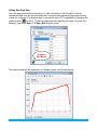
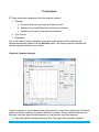
RESys
Reservoir Evaluation System
PT
Pressure Transient Analysis
Users Manual
Copyright 2006-2010, The Comport Computing Company
All Rights Reserved
RESys is an integrated software system for performing oil and gas reservoir evaluations.
Based on an integrated database and using object oriented software design techniques,
RESys is a modular and extensible software system consisting of various specialized
modules for the analysis and evaluation of well logs, core data, production data and more.
The modular integrated design allows the system to be extensible, so that additional modules
can be added without requiring a rewrite or redesign of the rest of the system. In addition, due
to the modularity and integrated database, individual modules can be optimized.
RESys is designed as a standalone, yet integrated system. Each module can be used by
itself; however the full power of integrated software is unleashed when the various modules
are combined.
PT comprises the module allowing the analysis of pressure transient well tests. As a
standalone program, it allows the evaluation and organization of well test data and
interpretations, but PT is fully integrated with the production related modules in RESys, so the
interpretations are available for use in an integrated evaluation of a reservoir or field.
At Comport Computing we value the comments and suggestions of our software users. If you
find a bug, please let us know. We'll fix it as fast as possible and send you a free updated
copy of the software. In addition, if you suggest an enhancement which we implement, you'll
receive a free upgrade to the new version.
Corrections or comments on RESys, PT or this manual should be directed to “[email protected]”.
Table of Contents
Overview............................................................................................................................1
Getting Started...................................................................................................................3
Creating a Project ..........................................................................................................3
Opening an Existing Project ...........................................................................................3
When a Project is Opened the First Time ......................................................................4
Creating a Well...............................................................................................................4
Creating a Well Test.......................................................................................................5
Importing PT4 Well Tests ...............................................................................................6
Entering Pressure Data ..................................................................................................6
Importing Pressure Data ................................................................................................7
Editing Raw Gage Data ..................................................................................................8
Entering Test Rates .......................................................................................................9
Fluid and Rock Properties ............................................................................................11
Test Analysis ...................................................................................................................13
Classical Cartesian Analysis ........................................................................................13
Classical Semilog Analysis ..........................................................................................14
Classical Square Root of Time Analysis ......................................................................15
Type Curve Analysis ....................................................................................................15
Regression Analysis.....................................................................................................16
Well Test Design..............................................................................................................18
Technical Description ......................................................................................................19
Fluid Types and Pseudopressure.................................................................................19
Pressure Transient Equations ......................................................................................21
An Overview of Pressure Transient Methods ...............................................................23
Computation of Pressure Derivatives ...........................................................................24
Overview
PT is a system for organizing and analyzing pressure transient well test data and
interpretations. The system consists of a database along with tools to aid in the entry of data
and interpretations. RESys is based on so-called “projects” which represent data that are
somehow related. You can create as many projects as you want and organize them in
whatever way makes sense for your purpose. For example, for pressure transient data,
perhaps a project would consist of all of the tests in a given oil field. On the other hand, for a
student, a project might be all of the tests done during a class or in conjunction with a project.
It really is up to you as to how you want to organize your projects and data.
It is important to understand that the project database contains all of the information needed
for well test evaluations. If you need to make a backup of the project, simply copy the project
database.
Once a project is created or opened, the leftmost side of the PT main window shows the list of
wells included in the project. To the right of the wells a list of well tests is shown. At the top of
the window there are various menus and tool bar buttons as shown in the screen shot below.
Selecting any well in the list will display the list of well tests available for that well.
The menu at the top of the window allows access to the functions available in PT and
includes functions to create and open projects, wells and well tests, etc.
The Toolbar contains buttons for rapid access to well test data and analysis functions, such
as viewing data entry, various analysis methods, etc.
The Project menu contains functions to create, open and close projects, and edit project
information.
The Data menu contains functions to create and edit wells, well tests, and test data.
PT User's Manual
Page 1
The Analysis menu allows the various analysis methods to be chosen.
The Design menu allows the design of well tests.
The Configure menu provides the option to automatically load the last project when PT is
started.
The Language menu allows the use of either English or Spanish text on all of the windows in
PT. To change the language, simply select the desired language from the menu.
The Help menu allows information concerning the version of PT to be displayed. To see the
version information, select Help | About.
PT User's Manual
Page 2
Getting Started
To start using PT, it is necessary to open or define a project. Defining a project creates a
database which will contain all of the data needed to evaluate well tests. It should be noted
that RESys uses a Microsoft Jet database by default. That means that there's nothing special
to install or configure, since Jet drivers are normally included in Microsoft Windows. It‟s the
same database format used by Microsoft Access. Once any RESys module, including PT, is
installed, it is ready to use without any further hassles, unless you decide to use a different
database format. The remainder of this manual assumes that the default Jet database is
used.
Creating a Project
To create a new project, select Project | New from the menu. You will need to select a
directory and a filename from the file selection dialog, and then will be asked if you want to
create the project. Selecting Yes will automatically create the database, selecting No will
abort with no database created. If the selected file already exists, you will be asked whether
to replace the database. Selecting Yes will overwrite the existing file, erasing all of its
contents. Selecting No will abort without doing anything.
Once the project database is created, you will be presented with a dialog to enter the project
name as shown. Simply add your own project title. Click Ok to save the project data or
Cancel to accept the default. Normally you will want to provide your own name for the project.
If you need to change the project name later, simply select Project | Edit from the menu.
Once the project has been created, it will be opened for use.
Opening an Existing Project
If you have an existing RESys project, you can open it for use by any module, including PT.
Simply select Project | Open from the menu and then choose the project database file from
the file selection dialog.
PT User's Manual
Page 3
When a Project is Opened the First Time
The first time a module is used with a particular project, the RESys system will check to make
sure that all needed parameters and units are defined and you will be presented with a dialog
allowing the units to be defined, as well as a dialog allowing the parameters to be defined.
Depending on what modules may have been used before, you may see some or all of the
following unit and parameter definitions. To accept the defaults, simply press Ok. To change
the default units, select or type the desired unit name in the Unit column and a conversion
factor in the Factor column. For example, to specify depth in meters, use m as the unit name
and 3.28084 (the number of feet in a meter) as the factor. To change the default parameter
values, type the necessary values in the respective Value column.
Note that once set, these values and units definitions cannot be changed, since doing so
would corrupt the database.
After the units have been set, PT uses two parameters that will need to be defined. As shown
in the above dialog, the Standard Temperature and Pressure are required and will be used in
volume calculations, especially for gases.
Creating a Well
Of course a project isn't of much use without data, so normally the next step will be to create
a well. Simply select Data | Well | New from the menu and enter the descriptive information in
the Well Data dialog. (Note that the Outcrop check box is not used in PT and should be left
unchecked.)
If you need to change the information later, simply select the well from the list and then select
Data | Well | Edit from the menu. Wells can also be deleted by selecting the well from the list
and then selecting Data | Well | Delete from the menu.
PT User's Manual
Page 4
Creating a Well Test
To create a new Well Test, select Data | Test | New from the menu and enter the basic
information in the PT Test dialog. If you need to change the data later, select the well test
from the right panel of the main form and then select Data | Test | Edit. Similarly a test can
be deleted by selecting the test and then selecting Data | Test | Delete from the menu.
PT User's Manual
Page 5
Importing PT4 Well Tests
If you have data from a previous version of PT, it is possible to import the data for use in
RESys PT, however there are several differences between the data used in previous
versions, so some rearrangement will be needed. To import PT4 data saved in *.dat files,
select Data | Test | Import PT4 File from the menu and then select the files to be imported. If
it doesn‟t already exist, a “pseudo-well” named PT4Import will be created and the imported
test data will be added to that “pseudo-well”.
Note that since PT4 did not explicitly store a test date, all of the imported tests will have the
current date, which can be corrected by editing the test data.
To associate the tests with actual wells, it may be necessary to create the wells as described
above. The tests can then be moved from the PT4Import well to the correct well by dragging
the test onto the desired well with the mouse.
Entering Pressure Data
Once a well test has been defined, time and pressure data will normally be entered. In PT
there are two options: 1) entering data manually, or 2) importing data from a pressure gage
data file.
To enter the data manually, select the well and well test, then select Data | T, P Data | Edit
from the menu. A dialog will be displayed where the data can be typed in manually, as shown
below. To accept and save the data, press the Ok button.
In many common cases, pressure transient data may be available in an Excel TM spreadsheet.
Note that the Excel data must be in 2 columns representing time in decimal hours and
pressure. To quickly copy time and pressure data from Excel to PT, select the data in Excel
and copy (Ctrl+C), then select the P, T Test Data grid and press Ctrl+V. The data will be
automatically pasted into the data entry form.
PT User's Manual
Page 6
Importing Pressure Data
In most cases it is much easier to import massive amounts of pressure data directly from a
pressure gage data file. Any data file that lists time and pressure in columnar ASCII format
may be imported directly into PT. To import test data, select eh well and test on the main
form, then select Data | T, P Data | Import Gage Data from the menu. On the file selection
dialog, select the file containing the data and press the Open button. The file will be read and
the Import Gage Data dialog will be displayed, showing the import parameters and a preview
of the data file as illustrated below.
The file preview shown in the bottom half of the dialog displays the line numbers followed by
the data. Before importing, select the number of lines at the start of the file to ignore, the
column numbers for the time and pressure data, the time format, and any desired thinning
parameters. By default no data thinning is performed, but in the case of large data sets, the
data can be thinned by specifying a maximum time interval and a minimum pressure interval.
For the values of Max DT = 1 and Min DP = 10 as shown in the example, at least 1 point will
be read every hour, but points less than 10 psia different will be discarded.
Once the import parameters have been set, press the Ok button to import the data. Once the
data has been read, the data editing dialog will be displayed where further data editing can be
performed, such as the removal of extraneous points before or after the actual test
information, i.e. when the gage is being run in and out of the well.
PT User's Manual
Page 7
Editing Raw Gage Data
Once the gage data has been imported, it is often necessary to edit the data to remove
extraneous data, such as spurious data points and pressures representing the gage running
in and out of the well. The simplest way to accomplish that in PT is graphically by pressing the
graphics button
on the P, T Data form displayed after importing the data. If the form isn‟t
showing, then select Data | T, P Data | Edit from the menu.
Graphics
Edit Button
The pressure data will be displayed in a Cartesian graph, as illustrated below.
PT User's Manual
Page 8
In the example, the actual data of interest begins at 1 hour and ends at around 6.5 hours and
consists of 6 increasing injection rates followed by a short fall-off. The data before 1 hour
includes pressures measured at the surface and while running the gage in the well, including
gradient stops. The data after about 6.5 hour includes data measured coming out of the well
and at the surface.
The data can be interactively edited using a variety of functions available on the buttons in the
toolbar at the top of the window. From the left side, the buttons perform the following
functions:
-
Mouse Zooms – puts the mouse in “zoom” mode and changes the cursor to 4
arrows. Dragging the mouse will select an area and zoom the display.
-
Mouse Selects – puts the mouse into selection mode and changes the cursor to
cross-hairs. This is the default mode, where dragging the mouse selects all of the
points in the selected area.
-
Zoom Reset – Resets the scales on the display to show all of the data points.
-
Select All – Selects all of the points.
-
Clear Selection – Unselects all of the points
-
Invert Selection - Changes all selected point to unselected and vice-versa.
-
Delete Points – Deletes all of the selected points
-
Set Time 0 – Shifts all of the data so that the first point becomes time = 0 for the
test
-
Accept Changes – Applies the changes made so far and replaces the test data
with the currently displayed data points. This cannot be undone.
Undo Changes – Throw away any changes made since the last Accept Changes
After making any changes to the data interactively, be sure to Accept Changes
the P, T Test Data form by pressing the Ok button.
, then close
Entering Test Rates
All pressure transient well tests require a set of test rates to be defined. In PT the well
producing or injection rates are divided into two sets: the rate history prior to the start of the
test and the rates during the test. Note that in PT, production rates are defined as positive (+)
and injection rates are negative (-).
In PT the times for the rates are expressed as time intervals in the order of occurrence. For
example, in the illustration on the right below, 3 time intervals are shown before the test, each
lasting for 3 hours, followed by a shut-in, i.e. buildup. Only the data during the buildup was
recorded and can be analyzed in PT.
To enter the test rates, select Data | Rates from the menu and enter the rates in the Prior to
Test and During Test panels on the dialog as shown in the following illustration. Note that the
PT User's Manual
Page 9
following simple cases require the following rate data:
-
Buildup Test – Enter the producing time and producing rate Prior to Test and zeros for
During Test.
-
Injection Falloff Test – Enter the injection time and negative injection rate Prior to Test
and zero during Test.
-
Drawdown Test – Leave the Prior to Test columns blank and enter the production rate
at time zero During Test.
-
Injection Test – Leave the Prior to Test columns blank and enter the negative injection
rate at time zero During Test.
In contrast to previous versions of PT, multiple rates during the test can also be analyzed.
The following rates illustrate the case of a multiple rate injection test, with 6 increasing
injection rates (50, 100, 150, 200, 250, and 300), for 1 hour each. Following 16 minutes (0.28
hours) at the final rate (350), the well was shut-in and the pressure fall-off was also recorded.
By entering the data as shown below (assuming the well was static before the start of the
test), all of the data can be evaluated.
PT User's Manual
Page 10
Fluid and Rock Properties
Every pressure transient test needs rock and fluid properties in order to be analyzed and
modeled. In PT the rock and fluid properties are entered by selecting the well and test, then
select Data | Fluid/Rock from the menu. The PVT Data dialog will be displayed allowing the
type of fluid to be selected and the necessary fluid and rock property parameters to be
entered.
In PT there are 4 types of fluid that can be selected. For liquids either Normal Oil or
Compressible Oil can be defined, while for gases, either an Ideal Gas or Real Gas fluid
model can be selected. The data needed for each case is shown in the displays below.
In most cases a Normal Oil will be used, where the fluid is a slightly compressible liquid and
the formation volume factor, viscosity and rock compressibility are all that are needed. For
volatile liquids, a Compressible Oil can be selected, where a base pressure for the formation
volume factor is specified as well as the fluid compressibility. This model is rarely used and is
only applies to fluid where the formation volume factor varies significantly during the test.
For gas well tests, the choice of an Ideal Gas requires temperature, z-factor and viscosity
information and will result in the use of P2 (pressure squared) analysis. This is only valid for
low pressure gases.
For most gas well evaluations, the use of the Real Gas model is recommended, but it also
requires a table of viscosity and z-factor versus pressure.
More information on the fluid models and the use of pseudo-pressure can be found in the
Appendix.
PT User's Manual
Page 11
PT User's Manual
Page 12
Test Analysis
PT offers three main categories of well test analysis methids:
1. Classical
a. Cartesian analysis for storage and reservoir limits
b. Semilog (Horner and Miller-Dyes-Hutchinson methods)
c. Square root of time for fractured well evaluation
2. Type Curves
3. Regression
Any of the methods can be selected by choosing a well and a test, then selecting the
appropriate analysis method from the Analysis menu. The following sections describe the
various analysis methods in more detail.
Classical Cartesian Analysis
Cartesian analysis is a technique whereby the pressure vs. time data is plotted on a Cartesian
graph and a linear tendency of pressure with time is chosen. Theory indicates that here are
two main situations when a linear pressure vs. time behavior would be expected:
1) Early time wellbore storage dominated flow. The slope of the pressure change is
PT User's Manual
Page 13
proportional to the wellbore storage parameters.
2) Late time semi-steady state flow when the entire drainage area of the well is being
depleted. The slope of the pressure change is proportional to the drainage volume and
compressibility.
Cartesian analysis can be done by selecting Analysis | Classical | Cartesian from the menu.
The parameters calculated can be determined by selecting the desired method from the
Method drop down list. Since well tests rarely last long enough to estimate reservoir volume,
Storage is the default method.
A window will be opened displaying the graph of the pressure vs. time data. The user may
select points, fit a line to the selected points, and compute either the wellbore storage or the
reservoir drainage volume.
Classical Semilog Analysis
Semilog analysis methods rely on the observation that, for radial transient flow, the pressure
changes linearly with the logarithm of time. The most common analysis methods are
1) Miller-Dyes-Hutchinson (MDH) for wells with a single constant flow rate, i.e. drawdown
tests. Pressure is plotted versus the logarithm of flowing time.
2) Horner analysis for wells that were flowing and were shut-in, i.e. buildup tests.
Pressure is plotted versus the logarithm of shut-in time divided by total flowing and
shut-in time.
In both cases the slope of the pressure vs. log of time is proportional to the flow rate,
PT User's Manual
Page 14
permeability, thickness and fluid viscosity. In addition, the intercept of the logarithmic line is
an indication of the near wellbore damage (skin).
Semilog analysis can be done by selecting Analysis | Classical | Semilog from the menu.
Classical Square Root of Time Analysis
Square root of time analysis uses a graph of pressure versus the square root of time. This
usually applies only to wells with vertical hydraulic fractures where the early time transient
flow is dominated by linear flow into the fracture. The slope of the pressure versus square root
of time is proportional to the permeability and fracture length squared. Note that superposition
may be applied, but strictly superposition should only be used when there was short flow time
before a shut-in, as in a drill stem test.
Square root of time analysis can be done by selecting Analysis | Classical | Sqrt Time from
the menu.
Type Curve Analysis
Type curve analysis relies on the observation that the dimensionless parameters for time and
pressure consist of reservoir and well parameters multiplied by time or pressure difference, so
the logarithms of the parameters are the logarithm of time or pressure plus the logarithm of
the reservoir and well parameters. When the theoretical pressure versus time response is
PT User's Manual
Page 15
graphed on a log-log graph, moving the data is the same as varying the pressure and time
coefficients of the dimensionless parameters. The coefficients are comprised of reservoir and
well parameters, allowing permeability estimation.
Type curve analysis can be done by selecting Analysis | Type Curves from the menu. A type
curve set can be selected from the Type Curve drop-down list. Moving the mouse while
pressing the left mouse button will move the data points relative to the curves. Alternatively
the match point can be entered directly into the tD(1) and pD(1) boxes. Based on the position
of the curves, the permeability-thickness product can be estimated, while other parameters
can be estimated visually from the curves.
Regression Analysis
Regression analysis uses a nonlinear regression technique to fit a theoretical pressure
response curve to the observed pressure versus time data by directly adjusting the reservoir
and well parameters to minimize the sum of the squared errors.
Regression analysis can be done by selecting Analysis | Regression from the menu. The
desired graph display (cartesian, semilog or log-log) can be chosen from the Graph drop
down list. The points to be used in the minimization can be selected using the mouse.
The well and reservoir model to be used, as well as the parameters to be optimized, can be
selected from the tab sheets on the right. Selecting the check box next to a parameter will
perform a fit using that parameter alone. The curve fit button can be used to perform an
optimization using all the selected data points with respect to the selected parameters. The
number of points used and the standard deviation of the curve fit is shown in the bottom
PT User's Manual
Page 16
status bar.
PT User's Manual
Page 17
Well Test Design
PT can be used to design well tests by entering estimated reservoir and well parameters and
generating the theoretical pressure response. To use the test design features in PT, create a
well and test as explained in the previous section. Fluid and Rock properties as well as Rates
should be entered.
Once the basic test data has been defined, select Design from the menu. On the form, the
type of well and reservoir can be selected and the parameters may be adjusted to see the
expected pressure response. The pressure response can be used to help in test design.
PT User's Manual
Page 18
Technical Description
Fluid Types and Pseudopressure
PT is internally formulated in terms of a generalized pseudopressure, so that most types of
reservoir fluids can be properly handled. In this version of PT, the fluid systems supported are
„Normal Oil‟, „Compressible Oil‟, „Ideal Gas‟, and „Real Gas‟. The only difference between the
models is the definition of pseudopressure which is used internally.
As shown by P. S. Fair, “Investigation of the Diffusivity Equation with General PressureDependent Rock and Fluid Properties” (submitted to SPE Dec. 1991), the diffusivity equation
can be written in terms of a general pseudopressure function which applies not only to gases,
but to any type of fluid and rock system where the physical properties vary with respect to
pressure. The use of this general pseudopressure function greatly simplifies the formulation
of pressure transient analysis methods.
In PT, the form of the general pseudopressure function is
where c is an arbitrary constant.
Using this general definition, the typical types of fluids normally encountered in practice can
be handled by simply defining the appropriate relationships for density and viscosity for each
fluid type and then evaluating the resulting integral.
Normal Oil
The normal oil model uses the standard assumptions of constant fluid viscosity and small,
constant fluid compressibility. In this case the integral simplifies to
. Note that the
density ratio is the definition of Bo and defining the arbitrary constant c = 1 gives the standard
definition of dimensionless pressure. In this case, the pseudopressure and pressure are
identical.
Compressible Oil
In the compressible oil fluid model, we remove the assumption of small compressibility, but
still assume that both viscosity and compressibility are constant. The fluid density is given by
PT User's Manual
Page 19
the relation
, where cf is the fluid compressibility. In this case the integral can
be evaluated analytically and the pseudopressure becomes
Real Gas
In the real gas model, fluid density is expressed in terms of the real gas equation of state and
the viscosity is assumed to vary arbitrarily with pressure. Both the real gas z-factor and
viscosity must be specified versus pressure. To maintain consistency with the standard
literature definition of real-gas pseudopressure, a factor of 2 is introduced, so the arbitrary
constant c = 0.5. This yields the following expression for pseudopressure:
Ideal Gas
In the ideal gas fluid model, the z-factor and viscosity in the real gas model are assumed to
be constant. In this special case the integral can be evaluated directly, yielding a
pseudopressure function proportional to p 2. This gives the standard p2 formulation which is
commonly used for gas wells at low pressure. In this case the pseudopressure definition
becomes
PT User's Manual
Page 20
Pressure Transient Equations
The basic relations for pressure transient analysis consist of the diffusivity equation, to
describe flow within the reservoir, along with suitable boundary conditions, to describe flow at
the outer edge of the reservoir as well as into the wellbore. In most cases, the reservoir is
assumed to be infinite, so the outer boundary condition is especially simple.
To simplify and standardize the diffusivity equation and boundary conditions, dimensionless
parameters are defined. The definition of these parameters, expressed in Darcy units are as
follows:
Radius
Time
Pressure
Rate
Storage
As documented in the paper “Generalized Wellbore Effects in Pressure Transient Testing”
(Fair, SPE Formation Evaluation, June 1996), the general equations for describing flow into
and pressure transient behavior within the wellbore during single phase well testing are as
follows:
Skin
Reservoir Inflow
Wellbore
The solution of these wellbore equations, along with the appropriate form of the diffusivity
equation, yields the general relationships used in pressure transient analysis.
In addition, the common forms for the „phase redistribution pressure‟ function used in PT are
defined as:
Fair
Hegeman
Using either of these definitions, there is a linear early time behavior (in the absence of
momentum effects) which has the appearance of wellbore storage. This apparent storage is
defined as:
PT User's Manual
Page 21
Apparent Storage
Summary of variables used:
B Formation volume factor
C Wellbore storage parameter
Cm Wellbore momentum parameter
C Wellbore phase redistribution parameter
ct Total fluid compressibility
h Reservoir thickness
k Permeability
p Pressure
q Flow rate
r Radius
S Skin factor
t Time
x Length
 Phase redistribution time parameter
 Porosity
 Viscosity
Subscripts
a apparent
D dimensionless
f fracture
i
initial
o surface
t total
w well
 phase redistribution
PT User's Manual
Page 22
An Overview of Pressure Transient Methods
The mathematical basis of pressure transient analysis lies in the partial differential equations
of single phase fluid flow. Since we are concerned mainly with the pressure response at a
producing well during time periods when wellbore effects may be important, the radial form of
the diffusivity equation is usually used to model the reservoir flow behavior. Since wellbore
effects are important, mass and momentum balance relations for fluids in the wellbore
describe the wellbore boundary conditions. Since the reservoir is normally extremely large in
comparison with the size of the wellbore, an infinite reservoir is often assumed.
In order to keep from solving the equations for every combination of parameters that might be
encountered, the equations are generally expressed in terms of dimensionless quantities.
Except for a few unusual circumstances, the same set of dimensionless parameters are used
throughout well test analysis and are described in Appendix I.
Once the diffusivity equation and the associated boundary conditions are specified in terms of
dimensionless variables and a solution is obtained, the process of pressure transient analysis
becomes one of determining what values of the dimensionless variables and parameters are
needed to achieve a match between the theoretical solutions and the measured data. This
can be done in several ways, leading to the three major methods used in pressure transient
analysis and implemented in the PT software.
Classical analysis methods rely on the observation that portions of the theoretical pressure
solutions form straight lines when plotted versus some type of time related variable. The
Cartesian plot is useful at early times, when wellbore storage dominates and inflow from the
reservoir is essentially filling the wellbore. It is also useful at very late times, when production
is draining the reservoir and the average reservoir pressure is dropping with time. The square
root of time plot is useful when transient linear flow dominates, usually due to flow into a
vertical fracture intersecting the wellbore. The semilog methods are useful during transient
radial flow after wellbore effects have died out. In any of the methods, fitting a straight line to
the data is one way to determine the parameters required to make the solution match the
data. The slope and intercept of the fitted line are used to compute the physical parameters.
Type curve analysis relies on the observation that the dimensionless time and pressure
parameters consist of a constant term multiplied by real time or pressure and the fact that
multiplying numbers is equivalent to adding logarithms. When both the theoretical solutions
and data are plotted on a log-log graph, sliding the data vertically and horizontally is
equivalent to adding or subtracting logarithms and thereby adjusting the constant term of the
dimensionless parameters. When a suitable match is obtained visually, the parameters can
be determined from the ratio of the real and theoretical parameters at any point on the graph.
This is equivalent to fitting a line, except that curves are used and no assumption of linearity
in the solution is required.
The adjust and compare method, as implemented in PT, is more direct in determining the
parameters of the solution. Instead of changing the problem into one of finding a straight line
or matching some set of theoretical curves, the data and theoretical solutions are plotted on
the same graph and the parameters of the theoretical solution are adjusted until the best
match is obtained. Using this method, we are able to analyze data which exhibit no straight
line by any method, as well as in situations where no set of type curves has been prepared.
The values of the parameters of the theoretical solution directly determine the desired
analysis results.
PT User's Manual
Page 23
Computation of Pressure Derivatives
Although the technique is usually referred to as "pressure derivatives", the actual quantity
used in "pressure derivative" analysis is the derivative of pressure with respect to the natural
logarithm of time. This corresponds to the slope on a semi-log plot, which always has more
visual curve character than that of a log-log plot, since the process of taking the logarithm of
pressure differences also removes most character from the data. Before development of the
pressure derivative techniques, semi-log methods were deemed more reliable for transient
analyses due to this loss of characteristic curvature with log-log methods.
Unfortunately, taking the derivative of measured pressure data is not trivial. The simplest
approach would be to simply divide each pair of pressure readings by the difference in logtime, however, except for ideal data, the resulting values nearly always have a high degree of
scatter. The scatter is due to round-off and measurement errors and makes use of the
derivative information impractical.
A two point method for estimating a derivative is
, where p is the value
measured at time t. If we expand with a Taylor series and add a small error, we obtain
When the second derivative term is small, the error is dominated by
and since
should be
small, the error can be very large.
To counteract this problem, a more complex algorithm is always used in calculating pressure
derivatives from actual data. The scatter is reduced by using a higher order numerical method
and by forcing time increments to be of a minimum magnitude, thereby adding a smoothing
effect to the derivative data.
The algorithm used is a second order Taylor's series approximation to the derivative with nonevenly spaced points. To derive the algorithm, note that a Taylor's series approximation to
subsequent data points can be written as:
and
If we hypothesize a relation of the form
PT User's Manual
Page 24
we can substitute the relations from the Taylor series expansion for p(t+ti+1) and p(t-ti-1) to
yield an expression for the derivative in terms of the adjacent function values and the
constants A, B, and C. By comparing the expression, we require that the coefficients for all
terms be zero, except the coefficient of the first derivative term which should be 1, yielding 3
equations in A, B and C. By solving the three equations for the coefficients simultaneously, a
complete expression can be obtained.
In this formulation, the second derivative error term vanishes, so we have a formula that is
more accurate, but it is still susceptible to small errors in the data when ti-1 and ti+1 are
small. We get around that problem by placing a lower limit on the size of ti-1 and ti+1.
In effect, we use a more accurate difference formula to minimize estimation errors, but make
the differences larger to ensure stability.
In pressure transient analysis, instead of pressure derivatives, we are actually interested in
the semi-log slope, which is the derivative with respect to the logarithm of time. The practical
implication of that is the difference in t is replaced by the difference in log-time. Even though
time differences may be large, the logarithmic difference may be very small. In practice, we
usually specify that the ratio of two times used in calculating the derivative are at least 1020% different. This has the effect of requiring that the ti in the differentiation formula is on the
order of 0.1 at the smallest and is usually adequate for most test data.
We also can take advantage of the fact that
.
Applying this relation, the formula normally used in calculating pressure derivative data is
where ti-1 < 0.9 t and ti+1 > 1.1 t.
PT User's Manual
Page 25