Download [txt] - inive

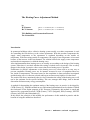
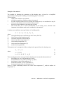
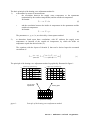
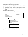
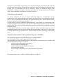
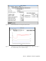
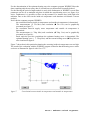
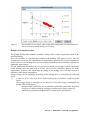
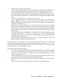
The Heating Curve Adjustment Method
Clima 2000 paper P343
topic 10 "Software"
W. Kornaat and H.C. Peitsman
TNO
Building and Construction Research
The Netherlands
The Heating Curve Adjustment Method
by
W. Kornaat
H.C. Peitsman
(phone +31 15 2608568, fax +31 15 2608432)
(phone +31 15 2608518, fax +31 15 2608432)
TNO Building and Construction Research
The Netherlands
Introduction
In apartment buildings with a collective heating system usually a weather compensator is used
for controlling the heat delivery to the various apartments. With this weather compensator the
supply water temperature to the apartments is regulated depending on the outside air
temperature. With decreasing outside air temperature, the supply water temperature is increased
because of the increase in the heat demand. The relation between the supply water temperature
and outside air temperature is called the heating curve.
After implementation these heating curves are usually set according to the design of the heating
system. Often there is no check whether this setting is indeed correct in practice. Due to safety
marges in the design, in practice often a some what lower heating curve is possible.
Furthermore in practice adjustments on the heating curves are often used as an easy way to
prevent complaints. Heating curves are for instance increased in case of complaints about too
low inside air temperatures. The actual cause for the complaints is often not further investigated
and the heating curve is often not set back and kept at an unnecessary high level in the future.
The result of the above mentioned is that in a lot of situations the setting of the heating curve will
not be the optimum for the specific building. This can, amongst other things, lead to thermal
discomfort and unnecessary energy consumption.
A method for determining the optimum setting of the heating curve in practice is developed by
CSTB (France) [1]. With this method an easy and rational optimalisation can be obtained. Within
the framework of the Sprint program of the European Community, this method is tested and
improved by cooperation between CSTB (France), CSTC (Belgium), IBP (Germany), SINTEF
(Norway) and TNO (the Netherlands) [2].
In this article the principle of this method, the performance of this method in practice and the
benefits of using the method are described.
Error! Unknown switch argument.
Principle of the method
The method for adjusting the parameters of the heating curve is based on a simplified
representation of the system : building / central heating plant / control unit.
This means that:
•
steady-state conditions are assumed;
•
a linear heat emission of the heat emitters is assumed;
•
no other terminal control devices (besides the heating curve) are considered or may be
active (e.g. all radiator valves need to be fully opened);
•
the effect of solar radiation is not taken into account.
This means that, for a correct determination of the heating curve, situations with
important solar radiation need not be considered for the analysis.
In steady-state conditions, an energy balance of a building yields :
G . V . (Ti - Te) = K . (Tw - Ti) + Ag
(1)
where :
G
is the global heat losses coefficient per cubic meter (W/m3.K)
V
is the volume of the heated zone (m3)
K
is the heat emission coefficient (W/K)
Ti
is the mean indoor temperature (°C)
Te
is the outdoor temperature (°C)
Tw
is the water flow temperature (°C)
Ag
are the free heat gains (W)
This equation can be arranged as follows, and gives the general form for a heating curve:
Tw = a . Te + b
(2)
a = - G.V / K
b = (G.V + K) / K . Ti - Ag / K
(3)
(4)
where :
This reasoning shows that an energy balance that takes into account the characteristics of
•
the building, by way of the parameters G and V;
•
the installation, by way of the parameters Tw and K;
•
the climate, by way of the parameters Te;
•
the thermal comfort, by way of parameter Ti;
•
the internal situation, by way of parameter Ag;
leads to a linear relationship between the water flow temperature Tw and the outdoor air
temperature Te.
Error! Unknown switch argument.
The basic principle of the heating curve adjustment method is:
1)
to determine by means of measurements:
•
the correlation between the supply water temperature to the apartments
(maintained by the weather compensator) and the outside air temperature.
In formula:
Tw = am . Te + bm
(5)
•
and the correlation between the inside air temperature in the apartments and the
outside air temperature.
In formula:
Ti = xm . Te + ym
(6)
The parameters xm, ym, am, bm, are derived by a least-squares method.
2)
to determine, based upon these correlations, with PC software the supply water
temperature as function of the outside air temperature, by which the inside air
temperature equals the desired value (Tc).
The equation (with the layout of formula 2) that can be derived upon the measured
correlations is:
Tw =
(xm - a m )
⎛ ( a m - 1).(T c - y m )
⎞
.T e + ⎜
+ b m⎟
⎠
⎝
( x m - 1)
( x m - 1)
(7)
The principle of the heating curve adjustment method is graphically illustrated in figure 1.
inside temp= f(outside temp)
30
supply temp= f(outside temp)
100
measured
25
measured
heating curve
80
20
60
desired value
15
optimum
heating curve
40
10
20
5
0
0
-10
-5
0
5
10
15
20
-10
-5
one or more
apartments
0
5
10
15
20
heating plant
front view
apartment building
figure 1:
Principle of the heating curve adjustment method
Error! Unknown switch argument.
Performance of the method in practice
The performance of the method in practice consists of 4 parts, namely:
1)
short term measurements (continuously monitoring) to determine the correlation between
(1) supply water temperature and (2) inside air temperature with the outside air
temperature;
2)
the determination of the current settings of the weather compensator;
3)
the construction of an input file, based upon part 1 and 2, suitable for the computer
program WINREG, by which the optimum heating curve will be determined;
4)
The analysis and the determination of optimum heating curve with the computer program
WINREG.
A flow chart of the method is given in figure 2.
The various parts of the method are in the following further discussed.
Short term measurements
Inventory of weather compensator
Parameters to be measured:
- supply water temperature of the weather
compensator
- inside air temperature(s)
- outside air temperature
For instance:
- current setting of heating curve
- period of night setback
- etc
Measuring time:
3 to 6 weeks (depending on variation in outside
air temperature.)
Construction of an input file suitable for
determination of the optimum heating curve
Using the computer program PREPATV(*) or
a common spreadsheet program all measured data
plus some extra information needs to be put in the
correct format.
Analysis and determination of the optimum heating
curve
Using the computer program WINREG(*)
(*)
figure 2:
both these computer programs are developed specific for the heating curve adjustment method
Flow chart of the heating curve adjustment method
Error! Unknown switch argument.
Short term measurements
The following parameters need to be measured:
1)
the supply water temperature to the apartments maintained with the weather
compensator.
This temperature can be accurate enough measured using an, at the outside well
insulated, surface sensor attached on the water pipe. This temperature needs to be
measured as close as possible to the sensor of the weather compensator. In this way also
the functioning of the weather compensator can be checked;
2)
the outside air temperature.
The outside air temperature needs to be measured on a location shielded from solar
radiation. It may be expected that usually a place besides the sensor of the weather
compensator will be correct;
3)
the inside air temperatures.
It is advised to measure the inside air temperature in the living rooms, because these are
commonly the most important and occupied rooms.
During the measurements the radiator valves need to be fully opened. This is done
because in this situation the weather compensator needs to be able to maintain the desired
inside air temperature.
The software developed for the heating curve adjustment method can handle a maximum
of 8 inside air temperatures measured in different apartments. Measuring in more
apartments, increases the accuracy of the method.
Furthermore by measuring in apartments spread over the apartment building (far and
close to the boiler room, on the top floor, the ground floor or an other floor, etc) an insight is gained in the thermal balance in the building. This means occur in different
apartments similar inside air temperatures. If this is not the case this can point out an
incorrect heat distribution (hydraulic unbalance), local unexpected extra heat losses or
local insufficient radiator capacity. These problems need to be tackled in general for
creating a good heating system and in special before an optimum heating curve can be
determined.
Because measurements need to be performed on various locations in the building (see figure 3), a
good option is to use several small one or multichannel data loggers. The installation effort per
apartment can then be minimized to about half an hour. Several different types of such data
loggers are nowadays available.
The measurements need to be performed during a period in which a sufficient variation in the
outside air temperature occurs on which a good correlation with supply water and inside air
temperatures can be made. In practice this comes down to roughly 3 to 6 weeks.
Error! Unknown switch argument.
heating plant:
• supply water temperature
• outside air temperature
apartments:
• inside air temperature measured in a maximum of 8 rooms
• with radiator valves fully opend
• by prefence measure in livingroom or kitchen
• selection of apartments:
- close to and far away for heating plant (in relation to
distribution heat losses)
- with high and low heat demand (apartments on top floor,
apartments in the middle of the buidling, etc)
- if possible apartments with complaints
figure 3:
Overview of measurements in front view of apartment building
Current setting weather compensator
outside air temperature -5C
supply water temperature (C
The current setting of the weather compensator needs to be determined, such as:
1)
the setting of the heating curve;
2)
limitations on the heating curve (e.g. 100
maximum limitation
maximum limitation at low outside air
temperatures, see figure 4);
80
3)
period with night setback;
60
4)
etc.
40
The setting of the heating curve is of course
needed to make a comparison with the measured
20
curve and to evaluate whether the weather
actual heating curve
compensator on this point functions correctly.
0
The other information is necessary to filter the
-20
-10
0
10
20
30
outside air temperature (C) -->
measured data. This filtering takes place during
the actual determination of the optimum heating
figure 4: Inventory of heating curve
curve with the computer program WINREG (see
later on). For this determination for instance only the measurements during the day are needed.
Based upon the period of night setback, the
Error! Unknown switch argument.
night period (with usually lower heating curve) and the heating up period at the start of the day
are determined and ruled out. During the day furthermore only the situations in which the actual
heating curve is functioning need to be considered. Periods in which the supply water
temperature is limited need not be considered (see figure 4). The measurements with limited
supply water temperature will make the correlation incorrect.
Construction of the input file
As already mentioned the use of several small data loggers is recommended for the
measurements. After performing the measurements, the data of these several loggers need to be
put in 1 file for further analysis concerning the optimum heating curve. Special attention hereby
needs to be given to the time synchronisation.
For this purpose a special computer program PREPATV is developed. For a description of this
computer program is referred to [3]. A few features of this computer program however does not
function well. This can give problems depending upon the used measuring equipment and actual
measuring results.
A more general option is to construct such an input file using a spreadsheet program. Often a
spreadsheet program is already used to visualize the measured data. In this case it is an easy step
to arrange the data in the spreadsheet to a format suitable for further optimizing of the heating
curve.
Analysis and determination of the optimum heating curve (WINREG)
The computer program developed for this purpose is called WINREG.
For a description of this computer program is referred to [4].
After reading the previous mentioned input file, this computer program first gives a window with
general information (see figure 5), such as:
location of the measurements (place name);
measuring interval (sampling rate);
number of measurements (number of samples);
period with night setback;
current setting of the heating curve (initial controller adjustment);
etc.
The measured data can be visualized with the program (see figure 6).
Error! Unknown switch argument.
figure 5:
General information concerning the measurements
T dep
T in1
T out
figure 6:
Visualization of the measured data in WINREG (T dep= supply water temp, T
in1= inside air temp, T out= outside air temp)
Error! Unknown switch argument.
For the determination of the optimum heating curve the computer program WINREG filters the
data, remaining only the necessary data. It is noted however that no data is actually deleted.
For the filtering the period of night setback is used, while furthermore in WINREG several filter
parameters can be set to maintain only data in which the actual heating curve (see figure 4) is
active. Furthermore it is possible to filter out days manual. For instance days with high solar
radiation. Due to the effect on the inside air temperature such situations can disturb a correct
analysis.
Next with the computer program WINREG:
the correlation between inside air temperature and outside air temperature is determined.
The measurements ( ∇ Tin Mes) and correlation („ Tin Corr) can be graphically
presented (see figure 7);
the correlation between supply water temperature and outside air temperature is
determined.
The measurements ( Δ Tdep Mes) and correlation ( Tdep Corr) can be graphically
presented (see figure 8);
based upon the previous correlations the optimum heating curve is determined. The
optimum heating curve ( ¿ Tdep New) and the current heating curve („ Tdep Init) are
also visualized in figure 8.
Figure 7 shows that in this particular situation the occurring inside air temperatures are too high.
The result of the evaluation with the WINREG program is therefor that the heating curve can be
set lower as illustrated in figure 8 with 12 to 17°C.
figure 7:
Correlation between inside air temperature and outside air temperature
Error! Unknown switch argument.
figure 8:
Correlation between supply water temperature and outside air temperature plus
the current and optimum heating curve setting.
Benefits of the method (results)
The primary benefit of the method is to obtain a setting of the weather compensator suited for the
specific building.
This will contribute to a good thermal comfort in the building. This means in cases, were the
heating curve was set too low, adjustments are determined to prevent too low inside temperatures
and in cases, were the heating curve was set too high, adjustments are determined to prevent too
high inside temperatures.
It is our finding that the heating curves in practice are mostly set too high, because adjustments
on the heating curves are often used as an easy way to prevent complaints about to loo inside
temperatures. In these cases optimizing the setting of the heating curve will also result in a
reduction of the energy consumption.
Energy savings, due to optimizing (lowering) of the heating curve, is realised by the following
issues:
1)
a reduction of the boiler heat losses (improvement of the performance coefficient of the
boiler).
This energy saving is determined to be about 2% of the total energy consumption for
heating. This is based upon:
•
the Dutch ISSO-publication 20, in which the performance coefficients for boilers
are given for various situations, amongst which the type of boiler control [5];
•
calculations performed with the model of a Dutch boiler manufacturer;
Error! Unknown switch argument.
2)
3)
a reduction of the transport heat losses.
From the Dutch ISSO publication 25 [6] is derived that the heat loss by transport pipes
can be reduced with about 20% in case the heating curve is reduced with 10 to 15°C.
The actual energy saving now depends per situation on the initial transport heat losses.
For an average Dutch situation we have determined that based upon 20% reduction of the
heat loss by transport pipes, about 1% on the total energy consumption for heating can be
saved;
a reduction of the temperature overshoot in the apartments.
Due to a high heating curve an overshoot of the air temperatures in the apartments is
possible leading to unnecessary energy losses. This overshoot is however hard to
calculate and depends on many things, as for instance: the control of the radiators, the
dimensions of the radiators, etc.
A part of this overshoot can however not be influenced by the users. This is the part
when the heat production, caused by the transport pipes in the apartments, exceeds the
heat demand of the apartment. The users can not control this heat production by the
transport pipes as they can control the heat production through the radiator by closing the
radiator valves.
For a typical Dutch apartment building is determined that in case the heating curve can
be lowered with about 10 to 15°C, an energy saving of 2% of the total energy
consumption for heating is reached due to preventing this overshoot that otherwise not
can be influenced by the users.
In practice higher energy savings are likely because overshoot in general (not only the
part that can not be influenced) will be prevented.
The sum of these 3 effects add up to a total energy saving of about 5% on the energy
consumption for heating, assuming a reduction of the heating curve with about 10 to 15°C. Our
research showed that such reductions are often possible. In case of higher or lower reductions the
energy saving are of course also higher or lower.
As additional benefits can be mentioned:
1)
the fact that insight can be obtained in the thermal balance between various apartments.
Or in other words whether or not similar inside air temperatures occur in various
apartments. If this is not the case this points to an incorrect heat distribution, local not
expected extra heat losses, etc.
If the thermal balance is not correct, based upon this insight, additional actions can be
performed to improve the functioning of the heating installation;
2)
the fact that by lowering the heating curve users will have less need to close the radiator
valves.
This will lead to a better functioning of the central control of the heating system.
Error! Unknown switch argument.
Demonstration of the method
The software programs will be demonstrated during the Clima 2000 congress.
Resume
The heating curve adjustment method provides an easy way to fit the heating curve for a
building, leading to an improvement of the thermal comfort within the building and/or reduction
of the energy consumption.
Due to the combination of measurements over a 'longer' period and analysis with computer
software, a rational adjustment can be determined and made. This is a large improvement in
relation with 'manual' adjustments, that are mostly used up to now, based upon occasional
findings and/or measurements.
It is indicated as an easy way because in total it will cost about 2 or 3 days per building to
perform the method. This means installing the measuring equipment, collecting and analyzing
the data, determining the optimum heating curve, removing the measuring equipment.
Furthermore there are little or no restrictions on the measuring equipment to be used. This means
that users can use their own equipment, with which they are familiar.
Due to the set up of the method and the guidelines, the method can also be used by people who
are less familiar with the technical aspects of heating plants. The method can therefor not only be
used by heating engineers and installers, but also for instance by building owners, municipal
energy managers, etc. This enlarges the possible use of the method in practice.
During our research in the Netherlands, it was our finding that the heating curves were often set
much too high. Lowering the heating curves with a least 10 to 15°C was possible in almost all
the considered apartment buildings. It is predicted that the use of the heating curve adjustment
method in such cases can lead to an energy saving for heating of about 5%.
Error! Unknown switch argument.
Literature
[1]
The heating curve adjustment system.
S. Nibel CSTB Paris, France
September, 1994
[2]
Transfer of a heating curve adjustment method and implementation with BEMS.
Final report.
EC-Sprint program Contract RA 159 ter.
March, 1996
[3]
PREPATV
User manual
Presentation and use of the software
March, 1996
[4]
WINREG
User manual
Presentation and use of the software
March, 1996
[5]
ISSO publication 20
Stichting ISSO, Rotterdam
[6]
ISSO publication 25
Stichting ISSO, Rotterdam
Error! Unknown switch argument.