Download to Model Documentation

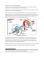
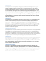
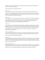
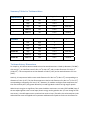
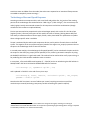
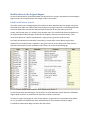
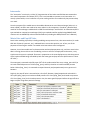
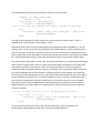
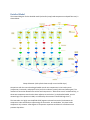
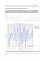
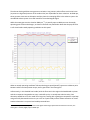
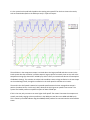
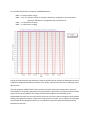
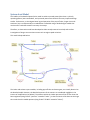
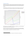
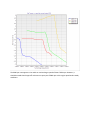
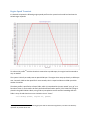
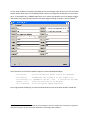
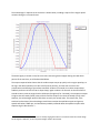
Turbocharged IC Engine Model This document describes two Sinaps‐based SINDA/FLUINT models of a turbocharged four‐cycle, inline six‐cylinder (3.7L) gasoline internal combustion (IC) engine. The purpose of these models is to demonstrate modeling capabilities and techniques. The models are intended to be representative of a typical design, but are otherwise notional. They are intended to provide starting points for a user requiring a more detailed analysis of an actual engine design. The reason why more than one model was created is that there are many areas of interest for such integrated turbocharger/engine simulations, from piston‐induced pressure waves to boost lag during acceleration. Therefore, both a detailed and a system‐level model were produced to allow focus on either short or long time scale events, respectively.* The first model focuses on the very short time‐scale events (< 1 second) including pressure waves in the intake and exhaust runners, and their effect on turbomachinery speed and performance. This detailed model could be extended to investigations of waste‐gate controls, EGR (Exhaust Gas Recirculation) transients, etc. The second model focuses on longer time‐scale events (> 1 second, up to ∞: steady‐state). This system‐
level model is appropriate for steady‐state sizing, or for simulating vehicle‐level transients such as boost lag or pop‐off valve actuation during throttle variations. In this system‐level model, an effective time‐
averaged engine representation is used to avoid resolving the details associated with resolving each crankshaft revolution, but the turbocharger and valve models are identical to those used in the detailed model. These models were developed as extensions of a model of a naturally aspirated (non‐turbocharged) engine design. Only those parts of the design and models that differ will be described here. The original model is documented separately (http://www.crtech.com/applications/ICengine.html). Basic knowledge of SINDA/FLUINT modeling is presumed. The model is built parametrically using “registers” (user‐defined parameters) whose names are indicated within the text using italics such as “Kair_filter.” Many variations can be made simply by adjusting these values, while others will require changes to the thermal/fluid network and associated user‐defined co‐
executing logic. The model was built using SI units, though some inputs were converted from English (US Customary) units. *
The temptation to do it all in one model should be avoided. A model built for short‐time scale events would be inefficient to execute for long time scales. A steady‐state model operates at infinite time scales, for example, and is an important tool for sizing and sensitivity studies. Compressor and Turbine Designs This section briefly explains the performance criteria and rationale for the compressor and turbine components for the IC engine/turbocharger thermal/fluid model. The design point was chosen as 4000 rpm, with intake at sea‐level and 25°C. It was desired to evaluate performance over the range of 2000 to 6000 rpm. One of the main reasons for an engine/turbocharger model is to verify the design of the combined system. Therefore, it may be no surprise that several iterations were performed on the turbine and compressor design before a satisfactory pair was chosen. It was decided to make all variations that were explored available to the user in the form of a Sinaps turbomachine library file (“tm_library.xml”). Therefore, a total of 5 compressors and 6 turbines are described below.† Turbocharger (Wikipedia.org) One way to evaluate a turbomachine within SINDA/FLUINT is to provide performance maps. For compressors, a map of pressure ratio vs. mass flow rate for several speed lines plus another map of isentropic efficiency vs. mass flow for several speed lines will satisfy this need. The edges of the pressure/flow map are assumed to represent choking and surge lines.‡ Similar maps are needed for turbines, as described in detail in the SINDA/FLUINT manual. The design concepts for all turbomachines presented herein were generated with the software packages known as CompAero and TurbAero. This software is offered by Turbomachinery Aerodynamic †
Not all of the turbomachines described have been placed into the Sinaps library. For example, it only contains low inlet temperature turbines. However, the raw data is available upon request, and it only takes a few minutes to cut and paste performance maps from an Excel sheet into the Sinaps tables. ‡
Surge lines can be identified separately if they do not exactly correspond to the edge of the map. Technology in Greensburg, Pennsylvania (www.turb‐aero.com). The proprietor is Ronald Aungier. Ron’s software enables representative design concepts to be generated and evaluated quickly.§ Cut‐away Turbocharger with Color‐coded Temperature Zones (Wikipedia.org) Compressor Design In total, five compressors were designed to support the modeling needs. Each was a single centrifugal stage with a basic volute‐type outlet. Initial estimates of the ingested air flow rate of 0.145 kg/s (0.32 lbm/s) in non‐turbo‐charged mode were used as a starting point (neglecting the boost in volumetric efficiency). This formed the “low flow rate” designs. Expecting a boosted intake pressure of twice atmospheric (2 bar), more compressors were designed for 0.29 kg/s (0.64 lbm/s). Finally, “medium flow rate” designs were added to allow additional pressure losses in air filters, mufflers, etc. Compressors were (for the most part) designed in pairs, with one compressor in a pair having a vaned diffuser, and the other a vaneless diffuser. The chief difference between these is that the unit with the vaned diffuser will exhibit somewhat higher efficiency in the area of design flow, but have a narrower range over which operation is stable. Compressors 1, 2, and 3 were designed for a boost of 83‐97 kPa (12‐14 psid) at the design point, while compressors 4 and 5 were designed for a somewhat higher boost of approximately 124 kPa (18 psid). It should also be stated here that in the interest of time, and given the demonstration nature of this modeling task, the efforts to optimize each unit’s aerodynamic design were not particularly strenuous. Several percentage points of efficiency could probably be realized with further refinement. §
CompAero and TurbAero input files corresponding to the machines in the library are available upon request. Other meanline turbomachinery software is available from other sources, and can be used as well providing performance maps can be created from them. Compressor #1 This compressor was sized to produce a design point mass flow rate of 0.145 kg/s (0.32 lbm/s) at a pressure ratio of approximately 2.0 Total‐to‐Total (T‐T). A relatively conservative value of design operating speed of 65000 rpm was chosen. Compressor impeller tip speed was set at 427 m/s (1400 ft/s). The compressor was equipped with a vaned diffuser to improve design point efficiency, and a conservatively‐sized volute. Efficiency at the design point is 66% T‐T. When operated with the IC engine Sinaps model, it was discovered that the design flow rate of 0.145 kg/s (0.32 lbm/s) was insufficient to support engine operation at the boost levels provided. The system model portrayed the compressor as operating perpetually in a choked state, which is physically consistent with what would be expected under these circumstances. Compressor #2 This compressor was sized to produce a mass flow of 0.29 kg/s (0.64 lbm/s) at approximately the same pressure ratio as compressor #1. Compressor #2 retained the same design speed (65000 rpm) as compressor #1. Compressor #2’s impeller tip speed was set at 427 m/s (1400 ft/s), identical to Compressor #1. It was also equipped with a vaned diffuser to improve design point efficiency. Design point efficiency is approximately 77% T‐T. The improvement over Compressor #1 is largely due to the increased mass flow rate. When operated with the IC engine model, compressor #2 experienced operation to the left of the surge line. Compressor #3 (Alternate) This compressor was sized to the same design point mass flow rate and pressure ratio as compressor #2. The design operating speed was also the same as compressor #2. However, a vaneless diffuser was substituted for the vaned diffuser of compressor #2. The vaneless diffuser resulted in a drop in design point efficiency to approximately 75%, but provided an increased stable flow range. Like compressor #2, #3 experienced surge at many steady state operating points portrayed by the system model. Compressor #4 This compressor was sized with a “medium” design point mass flow rate of 0.245 kg/s (0.54 lbm/s) and a higher design point pressure ratio of approximately 2.5 to better target the IC engine’s apparent air consumption characteristics. The higher pressure ratio was provided by an increase in compressor #4’s design speed to 75000 rpm. Compressor #4 also incorporated a vaned diffuser to raise design point efficiency, which was approximately 78%. Compressor #5 (Baseline) Compressor #5 was a counterpart of #4 with a vaneless diffuser to extend the stable flow range. Compressor #5’s design point efficiency was approximately 72% T‐T, due to both the vaneless diffuser and a reduction in design speed from 75000 to 70000 rpm (as needed to forestall the occurrence of inlet choking). In addition, the design inlet condition for Compressor #5 was changed to an inlet stagnation pressure of 86 kPa (12.5 psia), in order to better account for the presence of an air filter. Performance Map for Compressor #5 Turbine Design Before the turbine components are described in detail, a word about the turbine design philosophy is in order. Turbines were designed in pairs to support particular compressor component units. The difference between the two turbines in a pair (e.g., Turbines #1 and #2 constitute a pair) is the expected turbine inlet temperature. Due to uncertainties in the expected inlet temperature in this application, a “high” and “low” inlet temperature turbine was designed for each compressor. The “high” inlet temp turbine in a pair was designed for an anticipated turbine inlet temperature of 1220K (2200 R). The “low” inlet temp turbine in the pair was designed for a 695K (1250 R) inlet temperature. Each turbine of the pair was designed to be driven by the air mass flow rate that was supplied by the particular compressor that was being supported. In general, the design problem for each turbine was to find the turbine inlet pressure to be supplied by the IC engine to generate the required turbine power. The turbine exit static pressure was fixed at 105 kPa (15.2 psia) for all turbines except #5 and #6. These two units had their exit static pressures fixed at 124 kPa (18 psia), in accordance with data from previous IC engine model runs. The design power level for each turbine was set at 110% of the design point power for the compressor being supported. A 10% power “surplus” was enforced at the design operating point in order to require the turbine waste gate to be in some position other than fully closed. This provides the turbine/compressor power cycle with some nominal control authority. Note that when a turbine was designed to support either a vaned or vaneless diffuser compressor (compressors also tended to be designed in pairs) the turbine performance was designed to support the least efficient compressor of the pair at the design operating point. Note that all turbines were radial inflow turbines. Turbine #1 Turbine #1 was the “high” inlet temperature turbine of the two turbine units designed to support compressor #1. At the design speed of 65000 rpm, turbine #1 required an inlet pressure of 149 kPa (22 psia) total. This resulted in a design point pressure ratio of 1.45. Isentropic efficiency at this operating point was approximately 82% Total‐to‐Static (T‐S). Turbine #2 Turbine #2 was the “low” inlet temperature turbine of the two turbine units that supported compressor #1. At 65000 rpm, turbine #2 required an inlet total pressure of 203 kPa (29.5 psia) at 695K (1250 R) inlet temperature to generate the required power, for a design point pressure ratio of 1.94 T‐S. Isentropic efficiency at this point was essentially identical to turbine #1. Turbine #3 Turbine #3 was the “high” temperature turbine of the pair that supported compressors #2 and #3 (the “high flow” compressors). At 1220K (2200 R) inlet temperature, 65000 rpm, and design point flow rate of 0.29 kg/s (0.64 lbm/s), a turbine inlet total pressure of 176 kPa (25.5 psia) was required to generate the needed power. This implies a design point pressure ratio of 1.68. Isentropic efficiency at this condition was approximately 75%. Turbine #4 (Alternate) Turbine #4 supported compressors #2 and #3 at an inlet temperature of 695K (1250 R). A turbine inlet total pressure of 248 kPa (36 psia) was required. This resulted in a design point pressure ratio of 2.37, and an isentropic efficiency of approximately 82%. Turbine #5 Turbine #5 supported compressors #4 and #5 (the “medium flow” compressors) at an inlet temperature of 1220K (2200 R) and a design flow of 0.245 kg/s (0.54 lbm/s). A turbine inlet total pressure of 210 kPa (30.5 psia) was required, giving a design point pressure ratio of 1.69 at a speed of 75000 rpm. Isentropic efficiency was approximately 77%. Turbine #6 (Baseline) Turbine #6 supported compressors #4 and #5 (the “medium flow” compressors) at an inlet temperature of 695K (1250 R). A turbine inlet total pressure of 324 kPa (47 psia) was required, giving a design point pressure ratio of 2.61 at a speed of 70000 rpm. Isentropic efficiency was approximately 82%. Performance Map of Flows for Turbine #6 Performance Map of Efficiencies for Turbine #6 Summary Tables for Turbomachines COMPRESSORS Flow Rate Vaned Diffuser? Matching Turbine Usage Compressor #1 Low Yes 1 or 2 Compressor #2 High Yes 3 or 4 Compressor #3 High No 3 or 4 alternate Compressor #4 Medium Yes 5 or 6 Compressor #5 Medium No 5 or 6 baseline TURBINES Flow Rate Inlet Temp. Matching Compressor Usage Turbine #1 Low High 1 Turbine #2 Low Low 1 Turbine #3 High High 2 or 3 Turbine #4 High Low 2 or 3 alternate Turbine #5 Medium High 4 or 5 Turbine #6 Medium Low 4 or 5 baseline Turbomachinery Dimensions For simplicity, all turbines were assumed to have the same dimensions: a blade tip diameter (“DTURB”) of 9.4cm (3.7”), an inlet flow area of 1.85e‐3 m2 (1.99e‐2 ft2), and an outlet flow area of 2.13e‐3 m2 (2.29e‐2 ft2). This corresponds to an inlet diameter of 4.9cm (1.91”) and an outlet diameter of 5.2cm (2.05”). Similarly, all compressors had the same outlet flow area of 1.36e‐3 m2 (1.46e‐2 ft2), corresponding to a diameter of 4.2cm (1.64”). The low‐flow compressors had an inlet flow area of 1.46e‐3 m2 (1.57e‐2 ft2), corresponding to a diameter of 4.3cm (1.70”). However, for medium and higher flow compressors the inlet was raised by 30% (14% greater diameter) to avoid high Mach numbers at high engine speeds. When kinetic energies are significant, flow areas should be continuous: at a static (STAT=NORM) lump, if the two adjoining flow areas are not equal, kinetic energy can be gained or lost. (If a real change in flow area occurs, it should happen across a path and not across a lump.) Therefore, the turbomachinery inlet and outlet flow areas are applied to the upstream and downstream paths to make sure that flow area transitions were not hidden from the model, but rather were exposed as an intentional flow processes as needed to completely conserve energy.** Turbocharger Mass and Speed Response Assuming an aluminum compressor disc, and a steel shaft and turbine disc, the inertia of the rotating portion of the turbocharger was estimated to be 7.68e‐3 kg‐m2 (5.65e‐3 slug‐ft2). For convenience, this value (register inertia) was assumed constant for all compressor and turbine combinations (though variations of this number are explored below). Friction was assumed to be proportional to the turbocharger speed, with a value of 1.0e‐6 N‐m/rpm (register friction). Like many other parts of this model, this value is arbitrary (lacking better data) and acts mostly as a demonstration of how to apply friction, and a place‐holder for replacement or update when a design‐specific value is available. Torque is estimated by the turbine and compressor devices, and is positive for work done on the fluid system. The negative of the sum of these torques (stored as the register net_torque) represents the net torque on the turbocharger shaft if it were frictionless. In a steady‐state analysis, the turbocharger shaft speed (speedTC) can be varied until the point at which the torque on the shaft (net_torque‐friction*speedTC) is zero, either by parametric sweeps or by using the SINDA/FLUINT Solver in a goal‐seek mode. This method can be used to either verify system sizing, or for producing the initial condition needed to start a transient. In a transient, a first‐order differential equation (T = I*d/dt) can be co‐solved using the ODE utilities in SINDA/FLUINT. ODE #1 is initialized in OPERATIONS before a transient: call diffeq1i (1, speedTC*2.*pi/60., 0.0)
and is updated in FLOGIC 2 at the end of every time step: call diffeq1(1, stest, inertia, -friction*2.*pi/60., net_torque)
speedTC = stest/2./pi*60.
Note that the ODE is written in terms of radians per second, requiring conversion to and from revolutions per second (stest being a temporary variable containing the speed in rad/sec). **
The system‐level model permits one such hidden area change at the engine, resulting in a warning of “DISCONTINUITY IN FLOW AREA DETECTED” at the junction representing engine heating (where energy is imposed as a boundary condition, so it need not be conserved). Modifications to the Original Engine As was mentioned above, the detailed model was derived from a naturally aspirated (non‐turbocharged) engine model. This section describes the changes made to that model. Intake and Exhaust System The intake runners were enlarged slightly (from 45mm to 50mm diameter) but their length was greatly shortened (from 500mm to 150mm) given that tuning was no longer required in a turbocharged system. The box‐shaped intake manifold was replaced with an extension of the intercooler: a 61cm (2’, Lintake_man) long by 10cm (4”, Dintake_man) diameter pipe. This manifold (like the box‐shaped one in the original engine model) was again assumed to be stagnant, and was not resolved axially; it was assumed to operate as a perfect manifold with a single pressure, given the small L/D ratio. The intake duct became the intercooler (see below), so a new intake section (60cm long by 10cm diameter) was introduced, with a reduction in Kair_filter from 20 to 10 to keep the air filter pressure drop the same (despite a nearly twofold increase in flow rate, thanks to turbocharging). As with the naturally aspirated engine, the throttle is set to be wide open (unless otherwise indicated); engine speed variations are assumed to be caused by variations in the load. The exhaust system was largely the same in both engines, except that the irrecoverable losses (bends, etc.) in the muffler and exhaust pipe were reduced a little (as if the diameter had been slightly increased) to avoid another design iteration with the turbine. Intercooler The “intercooler” was simply a 1.22m (4’) long extension of the intake manifold that was assumed to have a wall temperature at ambient (25°C). This is not intended to represent a real intercooler: it is merely a place‐holder, since it achieves only minor cooling and has an unrealistically low pressure drop as a result. Since the purpose of the model was not intended to demonstrate a real heat exchanger (either air‐ or water‐cooled), no effort was made to be more realistic in this component. If need be, a detailed‐level model of a heat exchanger could be built in C&R Thermal Desktop® and FloCAD®. Or effectiveness/NTU‐
type methods or compact heat exchanger (CHX) type methods could be applied using SINDA/FLUINT routines such as HXMASTER, as documented elsewhere (including the SINDA/FLUINT User’s Manual). Waste Gate and Pop­Off Valve Detail valve modeling is possible, including modeling servo pressure lines, valve stem motions (2nd order ODE with frictional, hysteresis, etc.), tabulated losses versus valve position, etc. In fact, one of the purposes of these engine models is to enable valve interactions to be investigated. However, since these models are for demonstration and template purposes only, and since actual valve data is missing, the usual short cut of modeling a valve as an orifice is employed. Furthermore, a very simple control system is employed: flow area in proportion to the controlled pressure, with the pressure of the intake manifold being controlled by both the waste gate and pop‐off valve (also known as “blow‐
off valve”). The waste gate is assumed to be fully open (25% of the turbine outlet flow area, or Awg_open=0.25) at an intake manifold pressure of 2.2 bar (Pwg_open), and fully closed at an intake manifold pressure below 2.0 bar (Pwg_close). It is assumed to respond instantly and proportionately to any pressure in between. Similarly, the pop‐off valve is assumed to be a 2cm (0.8” diameter, Dpop) proportional valve which is 25% open (Apop_open) at an intake manifold pressure of 2.4 bar (Ppop_open) and closed at a pressure of 2.2 bar (Ppop_close). As the intake pressure rises, the waste gate fully opens before the pop‐off valve begins to open using these particular settings. The network‐based logic for the pop‐off valve (in FLOGIC 0) is shown below: if(pl#up .le. Ppop_Close) then
aori#this = 0.0
elseif(pl#up .ge. Ppop_Open)then
aori#this = Apop_Open*AF#this
c so not too wild, use proportional control instead of bang-bang:
else
aori#this = (pl#up - Ppop_close)/(Ppop_Open - Ppop_Close)
.
*Apop_Open*AF#this
endif
The logic for the waste gate is similar, except that since it controls a remote pressure, “pl#up” is replaced by the lump ID for the intake manifold, “pl150.” Why proportional control, and not just bang‐bang control (open/closed with a deadband, or “on‐off” control), which can be achieved by commenting out the last ELSE subblock in either the waste gate or pop‐off valve logic? The answer is primarily a matter of numerical convenience. Lacking more realistic valve response and control information, and remembering that these elements are merely place‐holders for a more design‐specific model, no effort was expended to model a more realistic control scheme. The response of the waste gate is critical, since the torques will balance at a partially opened waste gate position (see the steep portion of the net torque versus turbocharger speed plots in the system‐level model below, and see the comment on turbine 10% oversizing above). If a real waste gate were modeled including its complete dynamic response, the solution at the balance point might correspond to a time‐averaged position or flow resistance. A bang‐bang control system without any realistic lag would have no steady‐state solution (for the system‐level model) and would disrupt cyclic convergence (for the detailed‐level model). Even in a transient model of a realistic controller, proportional control must be present to generate useful initial conditions for the transient event, and it can be disabled during the transient. Using the SINDA/FLUINT NSOL flag to detect the type of the current solution, a slight modification of the valve logic that accomplishes this change from proportional to bang‐bang control is as follows: c so not too wild in steady-states, use proportional control:
elseif(NSOL .eq. 0)then
aori#this = (pl#up - Ppop_close)/(Ppop_Open - Ppop_Close)
.
*Apop_Open*AF#this
endif
For a more realistic model of a control valve, see the refrigeration cycle TXV example in the SINDA/FLUINT sample problem manual and in the Sinaps sample problem set. Detailed Model The network diagram for the detailed model (colored by lump/node temperature and path flow rate) is shown below. Sinaps Schematic (with cylinder heat transfer on an invisible layer) Comparison with the non‐turbocharged model reveals new components in the intake system (compressor, intercooler, and pop‐off valve) and in the exhaust system (turbine and waste gate). The mechanical connection between the turbine and compressor is “behind the scenes” mathematically, so these two components need not be shown adjacent to each other. (In the detailed model, see the network logic in the plenum air.1000, as indicated by the comment “Shaft ODE Logic here.”) The intercooler is a highly oversimplified HTNS (segment‐oriented convection) tie between the compressor outlet and the duct representing the intercooler. As noted above, this place‐holder component only removes a few degrees of compressor superheat and does not contribute much pressure drop either. The baseline compressor is Compressor #5, and the baseline turbine is Turbine #6 (described above). These are paths 125 and 225 respectively, so net_torque = ‐(air.torq125+air.torq225). Alternate turbines and compressors can be input or imported from the supplied library. The pop‐off valve flows from the intake manifold to the inlet of the compressor, and is controlled by network‐based logic in FLOGIC 0 (start of time step) as documented above. The waste gate by‐passes the turbine, and uses similar logic to the pop‐off valve to perform its control function as described above. Sample Results This section provides examples of the types of responses that are possible to explore for the detailed‐
level (short time scale) model. The pressures in the manifolds and runners (next to the valve) are plotted below for the 3000 rpm case. As expected, and by design, the variation in the pressure in the intake system is minimal. (Note that the intake manifold is low enough that both the waste gate and the pop‐off valve are always closed during this run.) The exhaust ducting exhibits strong pressure variations. Long runners and an effort to minimize losses (to preserve a high total pressure at the turbine inlet) are responsible for these variations. At 6000 rpm, these pressure waves are too disruptive and they lower the sweeping effect in the exhaust system: the unmodified exhaust system is not well tuned for the turbocharged engine. While the waste gate remains closed at 3000 rpm,†† it is partially open at 4000 rpm near the steady operating point of the turbocharger, as shown in the flow rate plots below. Note that the pop‐off valve is still closed under steady operating conditions at this speed. What are steady operating conditions? What turbocharger speed (speedTC) represents a balance point between turbine and compressor torque, and by‐pass flow in the waste gate? Unfortunately, in this detailed‐level model, with the flow rate in the engine calculated based on piston and valve responses integrated over many crankshaft cycles, no steady state solution exists. One alternative would be to run the model for a long time, starting with a good guess at speedTC or perhaps using artificially decreased inertia to try to arrive at a quasi‐steady answer without excessive run times. Another alternative is a system‐level model presented later. ††
At the steady‐state balance point, with a little higher turbocharger speed than the transient case uses, the waste‐gate is actually slightly open at 3000 rpm. It is the system‐level model which predicts the starting point speedTC for the short time‐scale results, such as shown below (back to the 3000 rpm case) in a plot of torques: The oscillation in the compressor torque is minimal due to the large manifold and short runners in the intake system. But the oscillation in turbine torque is large as pulses from each piston arrive, and as the temperature swings (by almost 30°C at 3000 rpm, which is likely an overestimate due to the assumption of adiabatic ducting). This variation in turbine inlet conditions causes a large oscillation in the net torque on the turbocharger shaft, though the oscillation in the shaft speed is small due to its inertia. The trend in the shaft speed is toward an increased speed because the time‐averaged net torque is positive (at about 0.6 N‐m in this case). Why? Because the initial guess at speedTC was too low. The system‐level model predicts an equilibrium point of about 57000 rpm. If this is the case, why not start at an even higher shaft speed? The reason is because the compressor is actually transiently surging at these conditions in the 3000 rpm case (but not at 4000 and 6000 rpm). This is shown by the LIMP indicator flag that SINDA/FLUINT produces to communicate the turbomachine status. For a variable‐displacement compressor (COMPRESS device): LIMP = 0: nominal (within range) LIMP = ‐11 or ‐12: speed is too low or too high, respectively, compared to input map values (pressures and flows are extrapolated, but not efficiencies). LIMP = ‐1: compressor is choking LIMP = ‐2: compressor is surging Letting the shaft speed increase would only make this problem worse. Instead, the waste gate control or compressor design would need more attention first. Finally, note that this case was run assuming a fully open throttle. Like most programs, SINDA/FLUINT cannot actually simulate a compressor during stall or recovery if such behavior is not already contained in the map (and that is almost never true, given the nature of the surge event). Instead, SINDA/FLUINT simply assumes that the edges of the valid map can be extrapolated into nearly flat curves of pressure ratio versus flow rate: that the compressor spins without making more significant progress in flow as the outlet pressure increases. This is evident in the flat spots at the bottom of the compressor efficiency, since efficiencies cannot be safely extrapolated past the boundaries of the map: In reality of course, the efficiency should drop precipitously when the compressor surges. The problem is more acute at 2000 rpm, and at that engine speed, turbocharger speed is also well below the available maps at about speedTC = 33000 rpm. Therefore, engine speeds lower than 3000 rpm were not investigated for the turbocharged engine detailed model with a fully open throttle.‡‡ This raises an issue: it is difficult to generate reliable performance maps far from the design point. To go too far away from that point, advanced compressor analysis methods or test data would be needed. By the way, for a turbine, LIMP has the following meaning: LIMP = 0: nominal (within range) LIMP = ‐1 or ‐2: pressure ratio or difference is too low or too high, respectively LIMP = 1 or 2: flow rate is too low or too high, respectively LIMP = ‐11 or ‐12: speed is too low or too high, respectively Is the use of steady‐state performance maps for the turbine and compressor during a short time‐scale event (such as those depicted above) acceptable? One answer is “yes” simply because the alternatives are virtually unavailable for any system‐level investigation (transient aerodynamics using a CFD program ‡‡
In fact, at steady state the 3000 rpm engine speed case continues to experience compressor surge. To avoid this as an initial condition, the system‐level acceleration transient (described below) starts at an engine speed of 3500 rpm. not being feasible in such a study). But with high velocities and high blade speeds, the transit times for fluid particles though either of the turbomachines are fortunately short compared to the even the small time scales applied here. Recovery from a surge within these time scales is a different matter, but as noted above, simulating surge itself is not realistic: all that can really be accomplished is to flag the potential for it happening, and then alter the design to avoid it. And that is a valid purpose for this type of model. Overall Performance Metrics In the non‐turbocharged engine model, overall performance metrics were calculated at three engine speeds. These corresponding calculations in this model yield the following results: 3000 rpm 4000 rpm 6000 rpm Turbocharger Speed 56000 rpm 62000 rpm 72500 rpm Volumetric Efficiency 122% 130% 130% VE (local density) 81% 82.5% 87% Thermal Efficiency 40.6% 42.0% 36.7% 33% 27% 23% 97.9kW 145kW 187kW Coolant Load Power to Crank The volumetric efficiency (VE, register vol_eff) is now greater than 100% due to turbocharging. An alternate VE based on local densities (rather than atmospheric) is also calculated since it is useful as an input to the system‐level model as described below. This alternate VE is calculated as vol_eff_sys. The power developed by the engine is, of course, much greater than that of the non‐turbocharged engine, which could only produce 84kW of power at 4000 rpm: turbocharging has increased power production by 73% at the design point. System­level Model The inability of the detailed piston/valve model to achieve a steady‐state (other than a cyclically repeating pattern) was noted above, and yet steady states form the basis for many important design studies. Furthermore, to investigate boost lag and operation of the pop‐off valve, longer time scale transients (say 1 to 100 seconds) are needed than are feasible using a detailed engine model that resolves each crankshaft rotation into many time steps. Therefore, an alternative model was developed to allow steady‐states to be solved, and to allow investigation of longer‐term transient events such as engine speed variations. This model is depicted below: The intake and exhaust system models, including pop‐off valve and waste gate, are virtually identical to the detailed model. However, the detailed responses of the runners are considered negligible in the interest of simplification (see below). The volumes within the intake upstream of the air filter have also been neglected (using FLUINT “junctions” instead of “tanks”), as has the inertia of the ducts at the larger time scales that this model operates (using FLUINT “STUBEs” instead of “tubes”). The baseline compressor is still Compressor #5, and the baseline turbine is still Turbine #6 (described above). These are paths 3 and 4 respectively, so net_torque = ‐(air.torq3+air.torq4). As with the detailed model, alternate turbines and compressors can be input or imported from the supplied library. The boundary node labeled “speedTC” in the middle of the diagram is a postprocessing trick that enables the user to check the current turbocharger speed using hover text. The temperature of this node, which has no effect on the solution, is set to the register speedTC. (This trick is not necessary for plotting, since registers can be plotted directly.) Simplified Engine Model. It was desired to operate at long enough time scales that the actions of each piston and valve could be averaged into a steady flow rate and heating value. The engine flow rate is therefore predicted as a positive displacement compressor, using the intake VE values from the detailed model calculated using local densities (calculated in vol_eff_sys) in the intake manifold (versus atmospheric density, which is the basis of vol_eff in the detailed model). This VE is imposed as a function of RPM. The displacement of this “compressor” is the full engine displacement (divided by 60 to allow speed to still be specified in rev/min rather than rev/sec), and the speed of the compressor is the engine speed divided by 2, being a four‐cycle engine. (Dividing the displacement by the same factor of 2 would have achieved the same result.) The combustion heating is replaced by a heating rate that is assumed proportional to the engine mass flow rate. This is achieved by applying the imposed QL (heating rate, in Watts) on the engine outlet (junction #1). This heating rate is determined by a curve fit based on exhaust temperature heating predicted from the detailed level model based on a second‐order polynomial:§§ Qexhaust = Qe0 + Qe1*air.FR1 + Qe2*air.FR1^2
where “air.FR1” is the mass flow rate (in kg/s) of the engine, as represented by the positive displacement compression (path #1). The work that this “compressor” adds has already been considered in the effective exhaust heating in the detailed‐level model, so it is subtracted for the net junction heating term: QL = Qexhaust – QTM#this
where “QTM#this” is the net turbomachinery work imposed on “this” junction (engine exit point). This system‐level engine representation is not intended to be either a template or a recommendation. It was merely convenient, and since the focus of this model is on the turbocharger, further refinement was not deemed necessary. (See also the closing notes on a hybrid detailed/system model.) §§
These values are calculated using the Excel Solver and an RMS fit method, with double weighting applied to the design point of 4000 rpm. Parametric Sweeps Having achieved a model that is capable of solving for inexpensive steady‐state solutions, many such solutions can be explored at once using a parametric sweep. While any key variable can be swept,*** in this case a lot of information can be gained by exploring results as a function of turbocharger speed (speedTC). For example, below is a sweep of flow rates through the turbine and waste gate, plus pressure ratios across the turbomachines, for the 4000 rpm engine speed case with a wide‐open throttle (WOT): The waste gate opens at about 58000 rpm, and is fully open by 63000 rpm, successfully dropping the turbine pressure ratio as a result of its by‐pass action. A plot of the net shaft torque (net_torque) during the same sweep shows that the stable operating speed of the turbocharger is about 61000 rpm (where compressor and turbine torques are balanced). This value can be used as the starting point for the detailed‐level model above. ***
More extensive multi‐variate design space sampling and searching methods are available as well. Note the steep slope at the balance point: this corresponds to the active region of the waste gate, as intended by the turbine design. This steep slope also means that speed variations will be minimal if the engine operates at this point: the waste gate will regulate speed. Outside of this active control range, more rapid shaft speed changes can be expected. The plot below is the same information, but including the 2000, 3000, and 6000 rpm engine speed cases as well. The balance point at 3000 rpm is not much different than at 4000 rpm, but the 2000 rpm balance point is a very slow 33000 rpm. However, this data must be disregarded: a plot of the compressor LIMP factor shows the compressor is surging at nearly all points along the 2000 rpm line, and a re‐design of either the compressor or the waste gate controller would be needed to extend the operating range to such slow speeds. This was previously discussed in the detailed‐level model. Once again, as a result only speeds higher than 3000 rpm were investigated.††† †††
The 3000 rpm case is actually bordering on unacceptable. A starting speed of 3500 rpm was there used in the system transient to avoid compressor surge as an initial condition. The 6000 rpm case appears to be stable at a turbocharger speed of about 72000 rpm. However, it should be noted that the pop‐off valve starts to open past 75000 rpm at this engine speed under steady conditions. Engine Speed Transient It is desired to impose the following engine speed profile on the system‐level model and see how the turbocharger responds: To achieve this profile‡‡‡ with the throttle is assumed to stay wide‐open, the engine load is assumed to vary as needed. The system is initially at steady‐state at speed=3500 rpm. The engine then ramps up linearly to 6500 rpm over 3 seconds, holds at that speed for 3 more seconds, then it ramps back down to 3500 rpm within another 3 seconds. The above profile is specified as a Sinaps Table, which is interpolated in the case named “rpm_up” as a function of time. (It can therefore be easily altered to follow another profile.) This Table look‐up logic is placed in the global FLOGIC 0 block, using a library interpolation routine and the knowledge that the Table is Array #3 and that the current simulation time is “timen:” call d1deg1(timen, engine.a3, speed)
‡‡‡
This profile was chosen for model testing purposes and for demonstrating features, and does not obviously represent any realistic drive case. For the initial condition, the speedTC that balances the turbocharger must be found, as if the parametric sweeps shown above were run and SINDA/FLUINT itself were charged with finding the zero net torque point. To accomplish this, a SINDA/FLUINT Solver run is set up with speedTC as the sole design variable, with OBJECT=net_torque‐friction*speedTC and GOAL=0 (goal seeking), as shown in the form below§§§ Use of the Solver to find initial conditions requires a custom OPERATIONS block: call solver
$
call destab
$
call diffeq1i (1,
timend = 12.0
$
call transient $
find the balance point (solve for speedTC)
summarize the solver’s in the output file
speedTC*2.*pi/60., 0.0)
$ initialize the ODE
set the end time to 12 seconds
run the engine speed transient
At an engine speed of 3500 rpm, the Solver finds the balance point to be about speedTC=57000 rpm.
§§§
NERVUS is also set to 3 to avoid halting for nonconvergence, which can happen due to compressor surge/stall and (more rarely) due to valve open/close instabilities in off‐design initial conditions. The turbocharger’s response to the transient is shown below, including a reprise of the engine speed variation during the 12 second event: The boost lags by a second or two, but even more interesting events happen during the slow‐down portion of the transient, as will be described below. The torque response below shows that the turbine torque ramps up quickly as the engine speed up, so the lag in the above speed curve is due to shaft inertia primarily, and not due as much to the pressurization and heating of the exhaust manifold. At about 3.5 seconds, the turbine torque drops suddenly and starts to level off. But it drops sharply again at about 6.25 seconds. At the end of the 12 second transient, with the engine back to 3500 rpm (though only for 3 seconds), the compressor torque is higher than the steady (initial) value, while the turbine torque is less than the steady (initial) value. However, the turbocharger speed is back down to nearly the steady value. This means that, if the transient had continued, the turbocharger would have overshot the equilibrium point and gone to speeds well below 57000 rpm, and would have probably oscillated about the equilibrium point after experiencing this disturbance.**** ****
As will be shown later, the compressor is actually surging after about 11.5 seconds: either the control design for this engine is defective, or the compressor design needs to be revisited. The pressures and temperatures in the intake manifold are shown below. Notice that, in first few seconds, the temperature and pressure in the intake manifold actually drop (and, as will be shown later, the waste gate closes). This is caused by the boost lag: the engine is depressurizing the intake system faster than the compressor can replenish it. The turbine event at 3.5 seconds is hardly felt by the compressor, but it feels the second event at 6.25 seconds. These “events” are, of course, the opening of the waste gate and the pop‐off valve. At 3500 rpm, the waste gate is partially open. After it closes during the initial lag event, by 3.5 seconds the intake manifold pressure has risen again beyond its 2.0 bar trigger point and the waste gate begins to open again, this time in earnest. Flow is suddenly diverted from the turbine, dropping its torque. However, the shaft speed continues to rise and so the compressor continues to raise the intake manifold pressure to the next threshold: the opening of the pop‐off valve at 2.2 bar. These flows are shown below, with the manifold pressure reprised for reference: Unfortunately, the damage has been done. Residual inertia in the shaft, plus residual pressure and temperature in the intake manifold (perhaps due to undersizing the pop‐off valve and/or intercooler), causes the compressor to go into surge at 9 seconds. This happens 3 seconds after the engine began to slow down, as shown below. (The turbine LIMP flag shows that it is moving out of its given map range, and that extrapolations are being used, which are not much of a concern as is surge in the compressor.) As was mentioned before, compressor surge can be detected not simulated with confidence, so anything past 9 seconds should be disregarded. Instead, the control system and/or the compressor should be redesigned to avoid this situation. Nonetheless, it is interesting that the surge continues to happen long after the intake pressure drops and the pop‐off valve has nearly closed again. Possible Model Extensions This section briefly describes further work or model extensions that are possible (or even advisable). Variable Valves. As with the naturally aspirated engine, electronic valve operation and other variable valve mechanisms (like dual cams) could be investigated using the detailed model. Similarly, the engine itself could be easily modified to represent a diesel engine or an Atkinson/Miller engine for hybrid cars. Intercooler. For both the detailed and the system‐level model, a more realistic intercooler should be added, including thermal lags that are associated with a significant mass of structural material (and perhaps water, if a water‐cooled design is used). Control Valves. More detailed waste gate and Pop‐off models, including improved controls, could be added. This can be as elaborate as time‐dependent valve stem or gate motions. VGT. Variable geometry turbines (VGTs), in which the nozzle vanes are controlled to both improve performance and to eliminate the need for a waste gate, is an interesting extension (along with the requisite control system). In SINDA/FLUINT, this is accomplished by a using family of turbines in parallel (one for each vane position), interpolating between these fixed‐map turbines based on the current vane position. (This technique has also been used for variable blade angles in other types of turbines.) Alternatives to this interpolated approach include dynamically adjusting a single map using expressions and/or user logic, or perhaps avoiding maps altogether by using a concurrently executed meanline turbine program (e.g., TurbAero) to “serve” the current operating point at each time step or iteration. Integrated Meanline Programs. Extending the simulation to handle VGTs is actually just one reason to consider the integration of the models with meanline software that predicts turbine and compressor operating points (e.g., CompAero and TurbAero). A more urgent need is a combined design tool, which would help reduce the manual iterations needed to find and to verify a suitable turbocharger design for a given engine design and a given set of operational scenarios. In this mode, the actual turbine or compressor design itself might vary in between iterations (or between steady‐state or transient solutions), perhaps as driven by SINDA/FLUINT Advanced Design Modules such as the Solver and the Reliability Engineering module. Multiple Compressors and Turbines. Expanding to two turbochargers, whether in parallel (perhaps for packaging), or in series (perhaps to expand the range of boosted engine speeds to lower RPM, or to increase the boost at higher RPM), would be relatively trivial†††† to accomplish using the techniques demonstrated here. (Any number of shaft speeds can be solved simultaneously, whether in steady state balancing using the Solver, or in transients using multiple co‐solved ODEs.) EGR. Other system‐level transients and interactions could be explored, including EGR (exhaust gas recirculation) systems for knock avoidance and emissions control, perhaps integrated with Tflame adjustments (if a more complete combustion model were not also used). EGR systems can have strong and often adverse interactions with turbocharger design and operation. Hybrid Detailed/System Model. The system‐level model could not predict engine flows and exit temperatures, and the detailed‐level model is not efficient for predicting turbocharger balance points, which it often needs as an initial condition. These models were developed in parallel, passing data back and forth between them. In essence, the system‐level model was calibrated against the detailed‐level model. (A careful reviewer will note that these iterations were not completely closed.) Both models could be available as submodels within a single Sinaps model, automating the passing of data and iterative closure. Submodels can be turned on or off dynamically (within a single run) as needed. Rev 1 October 10, 2011 www.crtech.com ††††
Complete with extra check valves and other by‐pass controls.