Download User Manual

G. Tiana, F. Villa, Y. Zhan, R. Capelli, C. Paissoni, P. Sormanni and R. Meloni
Montegrappa 1.1
A Monte Carlo code for polymer simulations
User Manual
2
Montegrappa 1.1
Table of Contents
Introduction
6
Getting started
6
Quick installation
6
Custom installation
7
The main features of Montegrappa
The Monte Carlo Moves
9
9
The Optimization of the Potential
10
The Enhanced Sampling Algorithms
11
The Atom-Types
11
Input files
12
file.pol
12
file.pot
14
file.par
18
file.op
25
Output files
25
A tool to prepare the input files: Grappino
28
Tutorials
32
1. Plain MC sampling with given potential
32
2. Optimization of the potential with plain MC
33
3. Replica exchange with given potential
34
4. Optimization of the potential with replica exchange
35
5. Adaptive simulated tempering with given potential
37
6. Optimization of the potential with adaptive simulated tempering
37
3
Montegrappa 1.1
4
Montegrappa 1.1
5
Montegrappa 1.1
Introduction
MonteGrappa is a code to carry out Monte Carlo simulations of various models of
polymeric chains, including proteins, DNA, etc. It is thought to be versatile and efficient.
Versatile means that one is free to use any geometric model and many forms of the
interaction between monomers to describe the polymeric chain. For example, a protein
can be described through a Cα model as a chain of spheres, or at full-atom detail, or at
any intermediate degree of coarse-graining. Efficient means that several elementary
moves are implemented to allow a fast sampling of conformational space.
One of the main novelty of the code is the possibility to optimize iteratively the
interaction potential. This result is achieved performing slight changes in the initial
interaction potential and retaining only those modifications that lead to a better
comparison between some thermal averages, computed after the sampling, and
available experimental data provided by the user.
Moreover, in the code are implemented several algorithms to enhance the sampling and
fasten the crossing of energy barriers. These are Parallel Tempering (also known as
Replica Exchange) and Simulated Tempering.
The package contains three programs: - MonteGrappa, the Monte Carlo engine; - Grappino, a tool to create the input files for MonteGrappa;
- mhistogram, a data-analysis tool.
Getting started
The code is freely available under the GNU General Public License (http://www.gnu.org/
licenses/gpl.html) and is provided as a tar.gz file that must be unpacked.
To extract the archive, just type in your terminal
$ tar xvf montegrappa.tar.gz
$ cd montegrappa
Quick installation
The easiest way of compiling Montegrappa and Grappino is to execute in their root
directory
$ make
$ make grappino
A full installation requires both GSL libraries and the MPI environment to perform
Simulated Tempering and Parallel Tempering simulations. 6
Montegrappa 1.1
If this is what you need, please check these dependencies before installing the
software; the GSL libraries should be in /opt/local/lib and their headers in /opt/local/
include. If they are in a different path, modify the variables LFLAGS and CFLAGS
accordingly. Then, type in your terminal
$ make all
If the building was successfully performed, the binary files “montegrappa”,
“montegrappa_mpi”, “grappino” and “mhistogram” can be found in the ./bin/
subdirectory.
If you do not have GSL/MPI libraries, skip to the next section for a customised
installation.
Custom installation
The Monte Carlo code can be compiled without enabling some features. Furthermore,
tools can be compiled separately from the main software.
(1) MonteGrappa Single Core, no Simulated Tempering (no Parallel Tempering)
REQUIREMENTS: none.
$ make cleanobj
$ make
The executable “montegrappa” will be created in the ./bin/ subdirectory.
(2) MonteGrappa Single Core with Simulated Tempering (no Parallel Tempering)
REQUIREMENTS: GSL libraries.
$ make cleanobj
$ make version=STEMPERING
The executable “montegrappa” will be created in the ./bin/ subdirectory.
(3) MonteGrappa Multi Core with Parallel Tempering (no Simulated Tempering)
REQUIREMENTS: MPI environment.
$ make cleanobj
$ make version=MPI
The executable “montegrappa_mpi” will be created in the ./bin/ subdirectory.
7
Montegrappa 1.1
(4) To compile Grappino and mhistogram,
$ make cleanobj
$ make grappino
$ make mhistogram
8
Montegrappa 1.1
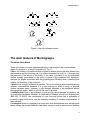
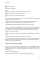
pivot
flip
multiple pivot
loose pivot
sidechain
multiple flip
centre of mass
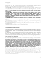
Figure 1: the set of allowed moves.
The main features of Montegrappa
The Monte Carlo Moves
There is a number of moves implemented in the code to explore the conformational
space of a polymer or of a set of polymers (cf. Fig. 1).
A flip is the rotation of a backbone atom chosen at random around the axis defined from
the preceding and the following one. It is efficient because it is local (i.e., it changes only
the positions of few atoms of the chain). In the case of proteins is not recommended
(unless strongly constrained by the option a_cloose in the parameter file) because it
changes the angles associated with the preceding and following atom, something that
violates the chemistry of the molecule.
A pivot move changes a dihedral at random. This is not effective when sampling among
compact conformations because it is a non-local move which is likely to produce
clashes between atoms. However, it only changes dihedrals of the backbone without
changing bond angles, which is good in the case of proteins.
A multiple pivot move is an extension of pivot moves, which changes at random a set
of consecutive backbone dihedrals. As illustrated in Shimada, Kussel and Shakhnovich,
JMB 308, 79 (2001), the combination of such non-local moves has a probability to
produce a quasi-local move, and the resulting sampling of compact conformations is
quite efficient.
A loose pivot move is a multiple pivot move such that the backbone atom following that
which defines the moved dihedral is kept fixed, varying in such a way the bond distance
9
Montegrappa 1.1
between the two. This move if exactly local and is reasonable if the variation of bond
lengths is controlled wither by a steep potential or by a sharp constrain.
A multiple flip consists in choosing two non-consecutive atoms of the backbone and
moving the backbone atoms in between around the axis defined by the two. As in the
case of a flip, this changes not only the dihedrals but also the angles involving the two
atoms chosen.
The local move described in the reference Giorgio Favrin, Anders Irbäck, Fredrik
Sjunnesson "Monte Carlo Update for Chain Molecules: Biased Gaussian Steps in
Torsional Space" J. Chem. Phys. 114 (2001) 8154-8158), modified to allow small
variations in the distance between the last moved atom and the first fixed atom (as in
the loose-pivot move).
A sidechain move consists in the random move of a sidechain among the allowed
rotamers.
If the system is composed of multiple chain, it is useful to make use of moves which
affect each chain as a whole.
The centre-of-mass move consists in the rigid translation of a chain or of a set of
interacting chains.
A rotation move of a chain or a set of interacting chains.
The Optimization of the Potential
This option is meant to optimize iteratively the two-body potential, in order to reproduce
the experimental values of conformational properties in terms of thermal-averaged
quantities.
To achieve this goal, a number (the keyword nrun in the parameters file, as explained
later) of conformational samplings is carried out. During each run, a set of
conformations is saved; the thermal averages relative to some meaningful quantities are
then computed from these data.
To perform the optimization a number of conformational samplings (nrun should be
larger than 1) is carried out. During each run a set of conformations are saved and on
these conformations the thermal averages relative to some meaningful quantities are
computed. These relevant quantities are chosen by the user, they must well describe
the system and their experimental values must be indicated in the file.op (see the
section “input file”). Then some elements of the matrix defining the two-body potential
are varied to optimize the chi squared between such thermal averages and the
“experimental” values contained in the file.op. The procedure is the one described in
Norgaard, Ferkinghoff-Borg and Lindorff-Larsen, Biophys. J. 94, 182 (2008).
The iterative procedure ends when the chi squared reached a threshold value defined
by the user, that is to say when a good agreement between experimental and computed
values is obtained. If this value is not reached the procedure stops after nrun.
An output file, called restrains_%d.dat, is printed at the end of each optimization. The
file contains the id of the experimental data, the calculated value, the experimental
value and the experimental error.
10
Montegrappa 1.1
The Enhanced Sampling Algorithms
Parallel Tempering (or Replica Exchange) is implemented as described in the paper
Sugita and Okamoto, Chem. Phs. Lett. 314, 141 (1999). With this technique N parallel
simulations are run at N different temperatures, settable by the user. All the necessary
keywords to set Parallel Tempering must be put in the file.par as illustrated in the “Input
files” paragraph.
Simulated tempering is implemented in its standard way (see Marinari and Parisi,
Europhys. Lett. 19, 451 (1992)) or in its adaptive version (see Tiana and Sutto, Phys.
Rev. E 84, 061910 (2011)). All the parameters which control the simulated tempering
must be set in the file.par as illustrated in the “Input files” paragraph.
The Atom-Types
In montegrappa the interaction potential is assigned between pairs of types: these can
be simply defined as atoms, but they can also be defined as chemical species or in
other ways. Thus we are in front of a generalization of the Go model, where the
interaction potential is always defined between pairs of atoms. The user can easily
choose how to define the types with the keyword atomtypes, that must be set in the
grappino input file. Setting atomypes to the value go the types are defined as atoms,
thus reducing the interaction potential to the one of the Go model. On the contrary, one
can indicate the path of a file.lib containing a specific type-definition for each atom;
grappino is able to read this file and to create an interaction potential following the given
instructions. The format of the file.lib must be the following:
itype
12
13
12
a_name
CA
CB
CA
aa_name
PHE
PHE
LEU
In the first column it is indicated the number identifying the type while in the other two
columns the names of the atom and of the amino acid are written. In this example the
same type has been assigned to the atoms CA of Leucine and Phenylalanine, thus
these atoms will interact with other types in the same way.
In the directory lib of montegrappa four files of this kind are available. These are:
1) atomtypes.1.lib, where each atom of each amino acid is defined as a different type,
with the exception of equivalent atoms (e.g OD1 and OD2 in aspartate).
2) atomtypes.2.lib, where atoms belonging to the same functional group, in different
amino acids, are assigned to the same type (e.g all the backbone-N atoms are of the
same type independently from the amino acid they belong to).
3) atomtypes.3.lib, where a CA model is considered
4) atomtypes.4.lib, where a N-CA-C model is considered
11
Montegrappa 1.1
The user is invited to read (and eventually personalize) these files in order to find and
specify a definition of types that is proper for the aims of his studies.
Input files
Montegrappa is launched with the command:
montegrappa file.pol file.pot file.par
where file.pol is the file which contains the geometric information about the topology of
the chain, about the initial conformation and about the possible rotamers of the side
chains of the polymer. The file.pot contains everything needed to calculate the energy of
the polymer, while file.par contains the parameters of the simulation, like the number of
steps, the temperature, etc.
Additionally the file.op is required when performing the optimization of the potential.
The structure of file.pol and file.pot is Gromacs-like, being divided in various sections
whose heading is contained in square brackets. Let’s see them in detail.
file.pol
The most important feature, concerning how the polymer is described in the code, is
that its backbone and its (eventual) sidechains are treated very differently. Here for
backbone we mean the atoms that are connected consecutively and whose movement
is the main responsible for conformational sampling. For sidechain we mean any atom
which does not belong to the backbone (like, for example, the carboxyl oxigen in an
amino acid).
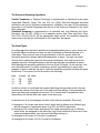
The first section of a file.pol is the description of the backbone, which looks like:
[ backbone ]
back
0
1
2
3
4
5
6
ia
0
1
2
7
8
9
13
type
N
CA
C
N
CA
C
N
itype
0
1
2
7
8
9
13
aa
VAL
VAL
VAL
SER
SER
SER
GLN
iaa
1
1
1
2
2
2
3
ch
0
0
0
0
0
0
0
x
22.3547
22.6948
23.556119
23.550922
24.688176
25.384945
26.797202
y
26.9596
27.49676
26.59827
26.88284
27.39688
28.35021
28.52898
z
tomove
61.6012
0
60.246765
1
59.400784
1
58.134317
0
57.288048
1
58.125661
1
58.369247
0
12
Montegrappa 1.1
The first column contains the identifiers (“back”) of the backbone atom. It runs over all
backbone atoms and must be unique in each separate chain. Within each separate
chain it starts from zero. The second column (“ia”) contains the atom identifier. It runs
over all atoms of the system and must be unique, even over different chains. In the
example, there are same gaps in the numeration of ia because the sidechain atoms are
listed in another section of the file.pol. While the numeration of the backbone atoms
must be ordered (i.e., consecutive backbone atoms must have consecutive backbone
id), this is not necessary for the atom id. The “type” column contains the nomenclature
of the associated atom and has the only purpose of being able to write pdb files. It is not
really needed by the Monte Carlo engine. The column “itype” contains a number which
identifies each atom type in terms of its interaction with other atoms. Pairs of atoms with
the same value of itype, respectively, interact in the same way. Different atoms can
share the same itype, and it has nothing to do with the string contained in the column
“type” (although a correspondence can be useful not to go crazy). The columns “aa” and
“iaa” contain the name and the number of the amino acid or of the DNA base; as the
name of the atom type, they are there only to be printed in the pdb file. The “ch” column
contain the identifier of the chain. There can be more disjoint chains, each with a
different “ch” identifier and with the “back” id starting from zero, while “ia” and “itype”
should run over all atoms independently on the chain id. The column “x”, “y” and “z” are
the cartesian coordinates of the backbone atoms in their initial condition. The last
column, “tomove” contains a binary variable which indicates if the dihedral and the
angle of that backbone atom can be moved (1) or must be kept fixed (0). For example,
in a protein, the omega dihedral, associated to each N atom, must not be moved.
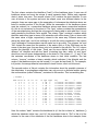
The second section of file.pol contains the information about the possible rotamers of
the sidechains. In montegrappa sidechains can only move in a discrete fashion among
the conformations (called “rotamers”) contained in this section. This is something like:
[ rotamers ]
back ch rot at
1
0 0 0
1
0 1 0
1
0 2 0
1
0 3 0
1
0 0 1
1
0 1 1
1
0 2 1
1
0 3 1
1
0 0 2
1
0 1 2
1
0 2 2
1
0 3 2
2
0 0 0
b1
2
2
2
2
0
0
0
0
0
0
0
0
7
b2
0
0
0
0
1
1
1
1
1
1
1
1
1
b3
1
1
1
1
4
4
4
4
4
4
4
4
2
ia type itype
4 CB
4
4 CB
4
4 CB
4
4 CB
4
5 CG1
5
5 CG1
5
5 CG1
5
5 CG1
5
6 CG2
6
6 CG2
6
6 CG2
6
6 CG2
6
3
O
3
ang
111.626220
111.626220
111.626220
111.626220
110.267281
110.000000
110.000000
110.000000
112.535141
110.000000
110.000000
110.000000
122.922219
dih
r
-128.612494 1.500833
-128.612494 1.500833
-128.612494 1.500833
-128.612494 1.500833
-57.012913 1.537856
175.000000 1.520000
63.000000 1.520000
-60.000000 1.520000
67.213399 1.537856
-60.000000 1.520000
-170.000000 1.520000
-292.000000 1.520000
-180.000000 1.229329
Here the column “back” contains the backbone id (cf. the first column in [ backbone ])
which the sidechain sticks from, and “ch” the associated chain id. “Rot” is the id of the
rotamer. In the case of the sidechain of the first backbone atom in the example, there
13
Montegrappa 1.1
are 4 possible rotamers, that are 4 possible conformations that such a sidechain can
assume. The backbone atom 2, which is the oxygen of the carboxyl carbon, has a
single rotamer, this means that its position is univocally determined by the position of
the associated backbone atom. The fourth column contains the id of the atom within a
given sidechain. In the example, the sidechain of the first backbone atom has 3 atoms
(each of them can be in 4 possible rotamers, for a total of 3x4=12 lines in the file).
The position of each sidechain atom is given in spherical coordinates. The columns
“b1”, “b2” and “b3” indicate which are the atoms (in terms of the atom identifier “ia”)
which form the basis set for the spherical coordinates. In the case of the first sidechain
atom in the example (the CB of the first amino acid), the atoms which build out the basis
set are b1=2 (that is, the C in the backbone), b2=0 (the N in the backbone) and b3=1
(the CA in the backbone). Since a basis set can involve also atoms in the sidechain, it is
necessary that an atom is defined previous than it is used as basis set. The atom id of
the sidechain is given in the eighth column, followed by the name of the atom (again,
useful only to write pdb files) and by “itype” which defines the kind of interaction with the
other atoms. The last three columns indicate the spherical coordinates, in terms of
angle (i.e., the angle between angles b2, b3 and the sidechain atom to be put), dihedral
(i.e., the dihedral between b1, b2, b3 and the sidechain atom to be put) and bond
distance (i.e., between b3 and the sidechain atom to be put).
The last section of file.pol contains the actual rotamer in which the sidechain of a given
backbone atom is in the initial conformation. For example,
[ sidechains ]
back
1
2
ch
0
0
irot
3
0
means that the sidechain of the backbone atom 1 of chain 0 currently occupies the
rotamer number 3 (defined by the set of spherical coordinates listed in the [ rotamers ]
section).
file.pot
This file contains all the information needed to define the interaction potential between
atoms. The basic interaction between atoms is a square-well potential of hardcore
radius rHC and width r, with a depth ε. Also this file is divided into sections.
The section [ global ] contains settings which affect all atoms. The keywords which can
be set in the global sections are:
14
Montegrappa 1.1
hardcore <double>
sets the default hardcore radius between any pair of
atom; is overridden by the value set in the [pairs] section
if this follows the global prescription in the file.
imin <int>
atoms of the same chain associated to backbone ids i
and j with |i-j|≤imin never interact according to the
instructions listed in the [pairs] section, but only with the
hardcore repulsion defined above.
e_dihram <double>
in case of ramachandran dihedral interaction (see
below), sets the energy scale which multiplies all
dihedral energies
homopolymeric <double ε
> <double r>
each pair of atoms interact through identical square
wells with given values of ε and r. It is overridden by the
instructions in section [ pairs ] if it follows the global
prescription in the file.
angle <double k> <double
α0>
sets a global harmonic potential in the angles of all
backbone atoms with harmonic constant k and rest
angle α0
dihedral1 <double k>
<double φ0 >
sets a global potential in the dihedrals φ of all backbone
atoms of the form k[1-cos(φ-φ0)]
dihedral3 <double k>
<double φ0 >
sets a global potential in the dihedrals φ of all backbone
atoms of the form k[1-cos(3(φ-φ0))]
splice <double k> <double
ke>
splice each square well defined in [pairs] into two parts.
The first part, between rHC and k*r mantains its depth;
the energy of the part between k*r and r is multiplied by
ke. Usually ke <1 to better approximate a Lennard-Jones
potential.
boxtype [c|s]
defined a cubic or a shperical box. Atoms are not
allowed to exit the box.
boxsize <double>
define the radius or the side length of the box.
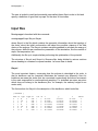
The most important part of the potential file is the [ pairs ] section, which define specific
square-well terms in the interaction potential between specific atom types.
15
Montegrappa 1.1
[ global ]
hardcore 2.000000
[ pairs
0
1
1
1
2
2
]
570
568
569
570
566
568
-1.000000
-1.000000
-1.000000
-1.000000
-1.000000
-1.000000
4.626141
4.547186
4.734172
4.347808
4.881537
4.758506
3.202713
3.148052
3.277504
3.010021
3.379526
3.294351
The first two columns indicate the atom type (“itype” in the file.pol). The other columns
indicate, respectively, the energy depth ε of the well, its width r and the width rHC of the
hardcore part of the well. It overrides the global keywords “hardcore” and “polymeric” if it
follows the global prescription in the file, but is always overridden by “imin”.
Angular potential between specific backbone atoms can be defined in order to keep the
angles near to their equilibrium positions. It is a sum of harmonic potentials. In the
file.pot they are defined as:
[ angles ]
ia
k
1
0.0100
2
0.0100
alpha0
106.452
115.721
where the columns are, respectively, the id of the atom (“ia” in the file.pol), the harmonic
constant and the rest angle in degrees.
Dihedral potential can be of two kinds: periodic or ramachandran.
The periodic potential is in the form:
k1[1-cos(φ-φ01)] + k3[1-cos(3(φ-φ03))]
where the id of the identifier of the atom (“ia”) and the four parameters k1, φ01, k3, φ03
are defined in the [ dihedral ] section, like:
[ dihedrals ]
ia
k1
2
0.500
3
0.500
phi01
160.000
160.000
k3
0.250
0.250
phi03
160.000
160.000
If this section is present, this kind of dihedral potential is active.
The Ramachandran dihedral potential is meant to favor alpha/beta secondary structures
propensities in proteins in an atom-dependent way. For a general dihedral angle φ (that
can be either the Ramachandran φ or ψ dihedral) the associated potential has the form:
εdih * pαia * fαφ(φ) + εdih * pβia * fβφ(φ)
16
Montegrappa 1.1
where the energy scale εdih is defined among the global parameters by the keyword
e_dihram. The weights pαia and pβia are the statistical weights indicating the probability
for the atom with identifier ia to be in alpha or beta conformation. The four functions
fαφ(φ), fβφ(φ), fαψ(ψ) ,fβψ(ψ) define the shape of the associated potentials: they are
gaussians with mean [φ,ψ]_[a,b] and standard deviation dev_ [φ,ψ]_[a,b].
To define this kind of potential, two sections are needed, [ Ramachandran_Dihedrals ]
and [ Alfa/Beta_propensity ]. They are in the form:
[ Ramachandran_Dihedrals ]
a/b phi/psi dev
mean
a
f
25.0
-57
a
p
30.0
-47
b
f
30.0
-129
b
p
35.0
124
[ Alfa/Beta_propensity]
iaa
a_prop
b_prop
0
0.000000
0.000000
1
0.007000
0.470000
2
0.058000
0.639000
....
The section [ Ramachandran_Dihedrals ] defines the mean and the standard deviation
(third and fourth columns) to use for the gaussian potential. These represent the ideal
phi(=0)/psi(=1) dihedral angle in an alpha(=0)/beta(=1) structured region.
The section [ Alfa/Beta_propensity ] defines the statistical propensities for alpha/beta
structure of each amino acid iaa.
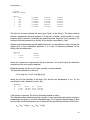
Another section that can be defined is [ hydrogen_bonds ], which turns an interaction
defined in [ pairs] in a directional interaction to mimic hydrogen bonds. It is in the form
[ hydrogen_bonds ]
ia
kind
other_ia
4
d
3
27
a
25
Each atom, defined by its identifier ia (first column) can be defined as an acceptor or
donor in the formation of hydrogen bonds (second column). The third column states to
which other atom each donor/acceptor is covalently bound (for example, a N in the case
of HN in a protein). If a pair of atoms defined in [ pairs ] are also defined, respectively,
as donor and acceptor of hydrogen bonds, the interaction energy defined in [ pairs ] is
multiplied by
( cos va * cos vd )1/2
17
Montegrappa 1.1
where va and vd are the unitary vectors defined by the acceptor/donor atoms,
respectively, with the atom covalently bound to them (e.g., the vector HN-N with the
vector O-C). If the global parameter “splice” is active, the range of the interaction is
defined only by the inner part of the square well (i.e., ksplice * r).
file.par
This file contains all the directives to carry out a Monte Carlo simulation with the system
defined by file.pol and file.pot. Additional parameters are required in the cases in which
the optimization of the potential, simulated tempering or parallel tempering are active.
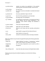
The general directives (valid in all the cases) are:
keyword
default
nchains <int>
compulsory
number of disjoint chains in the system
nstep <int>
100000
total number of steps of a run
nrun <int>
1
total number of runs to be done
seed <int>
-1
seed of random numbers (-1 means that
it is taken from the computer clock)
nprinttrj <int>
1000
every how many steps to print the
trajectory file
nprintlog <int>
1000
every how many steps to print the log file
nprinte <int>
1000
every how many steps to print the energy
file
traj <string>
traj
name of the trajectory file
logfile <string>
montegrappa.log
name of the log file
efile <string>
energy
name of the energy file
lastp <string>
last
name of the file.pol to write the last
conformation. If multiple runs, each final
conformation is file_%d.pol
procfile <string>
proc
name of the file relative to a given
process (MPI)
Temp <double>
1
the temperature of the simulation
debug <int>
0
0=silent, 4=every stupid thing
18
Montegrappa 1.1
keyword
default
flip <int>
no
try a flip move every <int> steps
pivot <int>
no
try a pivot move every <int> steps
mpivot <int>
no
try a multiple-pivot move every <int>
steps
sidechain <int>
no
try a sidechain move every <int> steps
lpivot <int>
no
try a loose-pivot move every <int> steps
mflip <int>
no
try a multiple-flip move every <int> steps
movebias <int>
no
try a local move every <int> steps, similar
to that described by Favrin et al. JCP 114,
8154 (2001)
movecom <int>
no
try a center-of-mass move every <int>
steps
moverot <int>
no
try a chain-rotation move every <int>
step.
dw_flip <double>
30
maximum width of a flip move
dw_pivot <double>
10
maximum width of a pivot move
dw_mpivot <double>
1
maximum width of a multiple-pivot move
dw_lpivot <double>
1
maximum width of a loose-pivot move
dw_mflip <double>
30
maximum width of a multiple-flip move
dx_com <double>
1
size of a center-of-mass move
dtheta
1
angular size of the chain-rotation move
nmul_mpivot <int>
3
number of consecutive dihedral to try in a
multiple-pivot move (a negative number n means: try a random number between 1
and n)
nmul_lpivot <int>
3
number of consecutive dihedral to try in a
loose-pivot move (a negative number -n
means: try a random number between 1
and n)
19
Montegrappa 1.1
keyword
default
nmul_mflip <int>
100
number of consecutive dihedral to try in a
multiple-flip move (a negative number -n
means: try a random number between 1
and n)
nmul_local <int>
9
number of consecutive backbone atoms
to move in local move.
bgs_a
200
amplitude parameter for local move
bgs_b
0.1
bias parameter in the local move
randdw <int>
1=flat distribution of random move,
2=gaussian distribution with stdev dw_*
r_cloose <double>
0.5
maximum variation of bond length in
lpivot moves, with respect to initial value
a_cloose <double>
-1
maximum variation of angles in flip and
multiple-flip moves, with respect to initial
value
d_cloose <double>
-1
maximum variation of dihedrals in flip and
multiple-flip moves, with respect to initial
value
nosidechain
no
avoid calculating sidechain energy if
there are none (to speed up)
noangpot
no
avoid calculating angular energy if there
are none (to speed up)
nodihpot
no
avoid calculating dihedral energy if there
are none (to speed up)
disentangle
no
allow moves among conformations with
overlaps, provided that the number of
overlap decrease
20
Montegrappa 1.1
keyword
default
always_restart
no
start each run from the conformation read
from the file.pol (instead than from the
last conformation of the preceding run)
hb
no
activate hydrogen bonds
stempering
no
activate simulated tempering module
shell
no
activates neighbour lists
nshell <int>
10
re-build neighbour lists every <int> steps
r2shell
6
radius of the shell which defines the
neighbours.
The number of chains, the temperature and the definition of the moves (flip, pivot, etc.)
are compulsory.
When performing the optimization of the potential in the file.par you should add the
instructions:
21
Montegrappa 1.1
op_minim <string>
none=do not perform any optimization of the potential;
sample=optimize the potential through a random search
op_file <string>
the input file.op
op_deltat <int>
how often to record a conformation to evaluate the thermal
average
op_itermax <int>
how many optimization steps on the chi2
op_print <int>
how often during optimization to print the status
op_step <double>
the energy step of the optimization
op_T <double>
the temperature corresponding to the experimental data (it
can be different from the actual temperature of the
simulation, since thermal average are calculated a
posteriori)
op_emin <double>
lower limit for any matrix element
op_emax <double
upper limit for any matrix element
op_wait <int>
discard the first steps and start recording conformations
later
op_rw
default width of energy well (if not defined in file.pot)
op_r0
default hardcore of energy well
record_native
activate first conformation (native) recording in simulation
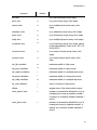
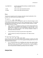
When the simulations are performed using parallel tempering the following parameters
must be set:
ntemp <int>
integer indicating the number of temperatures (=replica)
used. It must be equal to the number of processes.
temperatures
<double>
<double>
...
list of the ntemp temperatures (one for each line, with no
line-spaces)
step_exchange <int>
every how many steps trying an exchange between replica
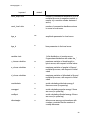
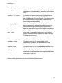
Finally, when performing the simulated tempering, one should set the following
keywords:
22
Montegrappa 1.1
23
Montegrappa 1.1
st_method <string>
stempering= standard simulated tempering, adaptive=
searches iteratively for the best choice of the temperatures
and the associated weights
st_nstep <int>
how often to attempt a temperature change
st_preamble <int>
how many steps perform to equilibrate
st_nprint <int>
how often to print the output
st_ntemp <int>
the number of different temperatures to be used (for adaptive
algorithm it is the initial number of temperatures)
st_temperatures
<double> [<double>]
<double> [<double>]
....
The list of temperatures.
For adaptive algorithm, initial temperatures.
For standard simulated tempering, the second [<double>]
number is the weight associated to that temperature.
st_debug <int>
The debug level (1-4)
st_nsadj <int>
how often to start the algorithm to readjust temperatures and
add new temperatures below (must be many times nstep, to
collect enough statistics)
st_emin <double>
the minimum energy of the collected histograms
st_emax <double>
the maximum energy of the collected histograms
st_ebin <double>
the energy bin of the collected histograms
st_anneal <string>
how to add a lower temperature at each attempt. Setting
<string>=prob it will be used a fixed exchange rate (see
st_lp_new).
Other features will be included in the next version.
st_lp_new <double>
exchange log-probability value (must be <0 !)
st_lpthresh <double>
log of minimum probability to remove a temperature; 9 to use
current probability
st_hthresh <double>
threshold on overall probability to keep an histogram (default
0.7)
st_keepall
use all past histograms to calculate thermodynamics
st_sumoldhisto <int>
if keepall active, keep only histograms of last %d run
st_ttarget <double>
target temperature, it is the temperature at which the system
is studied
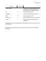
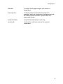
24
Montegrappa 1.1
st_printpdb <int>
print the output pdb after passing st_printpdb time at the
target temperature
st_tfile
name for the output temperatures.dat file
st_thefile
name for the output thermodyn.dat file
file.op
This file is not compulsory and is necessary only when using the optimization of the
potential. Such a file can be in two possible formats.
The former is:
i
j
kind value sigma
which means that objects i and j are expected to give rise a thermal average on some
conformational properties defined by kind, and the experimental value of this thermal
average which we would like to reproduce is value with a standard deviation of sigma.
The possible choices of kind are:
0
i and j are the id of a backbone and value is the contact function between the
former atom or any sidechain atom belonging to it and the latter, or any
sidechain atom belonging to it. The contact function takes the value 1 if two
atoms are in contact according to the two-body interaction defined in
potential.pot and zero otherwise.
1
i and j are atoms id (ia in the pol file) and value is their distance
2
i and j are atoms id (ia in the pol file) and value is 1/d6, where d is their
distance.
The other format of the file.op can be:
i1
j1
i2
j2
kind value sigma
which means that the conformational property to be calculated is between the whole
segment involving objects from i1 to j1 to the segment involving objects from i2 to j2.
The possible choice of kind is:
3
i1, j1, i2 and j2 are the id of a backbone and value is the contact function
between any atom of the former segment and any atom of the latter segment.
The contact function takes the value 1 if two atoms are in contact according to
the two-body interaction defined in potential.pot and zero otherwise.
Output files
25
Montegrappa 1.1
The main output files generated by the program are:
montegrappa.log
which contains some additional information on the
development of the simulation, depending on the debug
level
trajectory_%r_%p.pdb
It contains the trajectory, written as a multiple pdb file.
Each snapshot is separated by “ENDMDL”, in order to
be compatible with the gromacs tools. One trajectory file
is produced for each run (and also for each process
when using parallel tempering).
energy_%r_%p.ene
It is a file containing the number of step, the total
energy, the two-body energy, the angular energy and
the dihedral energy. One energy file is produced for
each run (and also for each process when using parallel
tempering).
last._%r.pol
at the end of a simulation (and of each run) it writes a
pol file containing the last snapshot, in order to be able
to restart the simulation.
When performing the optimization of the potential also these files are generated:
restraints_%r.dat
One file for each run. It contains the id of the
experimental restraints, the calculated value, the
experimental value and the experimental error.
newpot_%r.dat
One file for each run. It contains the data relative to the
optimized potential, obtained at the end of the run.
chi2.dat
Contained the value of chi2 obtained comparing the
computed averages and the known experimental values
at the end of each run.
Finally, the files produced in the case of Simulated Tempering are:
26
Montegrappa 1.1
dumb.dat
It contains the average energies as a function of
temperature.
thermodyn.dat
Containing all the fundamental thermodynamic
quantities, which are: temperature, average energy with
the relative standard deviation, specific heat, free
energy and entropy.
temperatures.dat
It reports the temperature at each step.
harvest.pdb
Contains the conformers saved at the required
temperature.
27
Montegrappa 1.1
A tool to prepare the input files: Grappino
Grappino is a tool which takes as input a pdb file and generates a pol and a pot file,
according to the instructions contained in a input-parameter file created for the purpose.
It is mainly thought for implementing Go models or similar. The command line is
grappino file.in
where the input file file.in contains the following instructions.
General section:
pdbfile <filename>
the name of the input pdb file containing the native protein
polfile <filename>
the name of the output pol file (default: polymer.pol)
potfile <filename>
the name of the output pot file (default: potential.pot)
contactfile <filename>
the name of an output file containing the contacts between
atoms in the pdb file
debug <int>
the debug level (1-4)
Polymer section:
hydrogens
if defined, keeps the hydrogens present in the pdb file
nosidechain
if defined turn off everything related to sidechains (that is, it
uses a CA model)
rotamers
if defined, use rotamers to define sidechains
model <modelname>
if defined, turn off the sidechains and it maintains 3 possible
models: CA, CACB and NCAC
rotfile <filename>
the path of the library containing the definition of rotamers
cb_pdb
if defined, instead of using the default position of the CB
atoms (hardcoded), use the position of the pdb
pdb_rot
if defined, uses the rotamer position in the pdb file
Potential section:
28
Montegrappa 1.1
backbone_atoms
number and name of backbone atoms (eg: 3 N CA C)
locked_atoms
locked atomtype in backbone
imin <int>
minimum distance between backbone atoms to define a
native interaction
r_hardcore <double>
the hardcore radius of the potential (in A°)
r_native <double>
the threshold distance used to define native contacts (in A°)
use_nativedist
if defined, set well width to experimental native distance
k_native_r <double>
in use_nativedist, multiply the native distance by this factor
k_native_hc <double>
in use_nativedist, multiply the hardcore distance by this
factor
potential [go]
initial potential
splice <double k>
<double ke>
splice each square well into two parts. The first part,
between rHC and k*r maintains its depth; the energy of the
part between k*r and r is multiplied by ke. Usually ke <1 to
better approximate a Lennard-Jones potential.
r_bonded <double>
the threshold to define a covalent bond, used to construct
the protein topology
go-energy <double>
the depth of the attractive well
atomtypes <string>
if the string is “go”, label each atom with a different type,
otherwise read the types from the file defined by the string.
The format of the file is “%d %s %s”, which contains the
numeric type to be used by grappino, the atom name and
the amino acid name (e.g. “17 CA GLY” sets the CA of
glycine to atom type 17)
go_dihedrals
define a dihedral potential based on the native conformation
go_angles
define an angular potential based on the native conformation
e_dih1 <double>
energy factor of the multiplicity-1 go dihedral potential
e_dih3 <double>
energy factor of the multiplicity-3 go dihedral potential
e_ang <double>
energy factor for the go angular potential
dih_ram
define a dihedral potential based on (ideal) Ramachandran
dihedrals
29
Montegrappa 1.1
e_dihram <double>
energy factor for the Ramachandran dihedral potential
phi_0_a <double>
ideal φ angle for α structures (default: -57°)
phi_0_b <double>
ideal φ angle for β structures (default: -129°)
psi_0_a <double>
ideal ψ angle for α structures (default: -47°)
psi_0_b <double>
ideal ψ angle for β structures (default: 124°)
sig_a_phi <double>
Standard deviation of φ angle potential for α structures
(default: 25°)
sig_b_phi <double>
Standard deviation of φ angle potential for β structures
(default: 30°)
sig_a_psi <double>
Standard deviation of ψ angle potential for α structures
(default: 30°)
sig_b_psi <double>
Standard deviation of ψ angle potential for β structures
(default: 35°)
propensity <filename>
the file containing the aminoacids α/β propensity (e.g.
PSIPRED output)
r_homo <double>
homopolymeric interaction width of the well (in A°)
e_homo <double>
homopolymeric interaction depth of the well (in A°); this is
anyway overruled by specific pair interactions
cys_e <double>
define a special well for cys-cys interaction, with this depth...
cys_r <double>
... and this width
Optimization section:
30
Montegrappa 1.1
op_file <filename>
name of the output file containing native restrains for the
purpose of optimizing potential
op_kind <string>
“GO_DIST_CA”=put a restraint on each pair of CA atoms
that are distant more than imin in the chain
“GO_DIST_ALLATOM”=consider, for each amino acid, the
CA atom and the last atom of the sidechain (the one with the
last id for the amino acid in the pdb file, excluding the carbon
C). The algorithm put a restraint on each pair of atoms
belonging to the selection, which are distant more than imin
in the chain. To reduce the huge amount of restraints
produced, the pairs are considered only if both the atoms
belong to an amino acid with even index (or if both belong to
an “odd” amino acid).
31
Montegrappa 1.1
Tutorials
1. Plain MC sampling with given potential
In this short tutorial MonteGrappa is used to make unfold and refold a small peptide of
64 aminoacids, namely a small domain of chymotrypsin inhibitor 2.
MonteGrappa needs three input files:
- a .pol file, which contains the topology of the polymer
- a .pot file, which contains the details of the potential
- a .par file, which contains all the other parameters
In this directory two .par files and are present, while the files .pol and .pot must be
created using the utility Grappino. Grappino needs a single input file (.in) and a
reference structure (.pdb): you can find both them in this same directory.
Now have a look at 1YPC-CA.in, the input file for Grappino: it tells to use the 1YPC.pdb
file as input in order to produce 1YPC-CA.pol and 1YPC-CA.pot (keywords pdbfile,
polfile and potfile, respectively). Then take a look also to the other parameters. With the
help of the Manual and the README.txt you will be able to understand that the peptide
is studied with a simple CA-model, in presence of a go-like interaction potential and with
an additional potential on the dihedrals.
Now run Grappino with the syntax:
$GrappinoPath/grappino 1YPC-CA.in
You should see 1YPC-CA.pol and 1YPC-CA.pot in this directory.
Now open 1YPC-CA.unf.par: you can see that we are simulating a protein for 5000000
MonteCarlo steps at a temperature of 1.6. Note that in MonteGrappa fictitious
temperatures are not easily referable to the real ones. Here, the values of the potential
are tuned in order to let the protein be stable at T=1 and unfold at T=1.6.
Run MonteGrappa (the single-core, not-stempering version!) typing:
$MontegrappaPath/montegrappa 1YPC-CA.pol 1YPC-CA.pot 1YPC-CA.par
with all the arguments in this exact order. After 5 millions MC steps, you should have in
your directory the following files:
- traj.pdb is the trajectory in the common .pdb format. It can be visualized by using
software like VMD.
- last.pol is the last-known conformation, in MonteGrappa format: it can be used as an
input for other simulations. In this version of the code, the last conformation is saved
only in .pol format, thus if you really need to visualize it via VMD you should refer to the
last frame of the trajectory.
- energy.ene contains total and partial energies for every MC step you chose to print at.
- montegrappa.log contains some information about the simulated system, the energy at
chosen MC steps and the acceptance of the move.
32
Montegrappa 1.1
Using gnuplot to see the energy vs time in energy.ene file with:
gnuplot> plot “energy.ene” u 1:2
you can easily check that energy indeed increases during the simulation. Furthermore,
you can calculate the rmsd between the whole .pdb trajectory and the reference
structure contained in the .pdb file.
NB: if you want to perform such a test, use the first frame of .pdb file as reference's file,
not the original .pdb structure file (here 1YPC.pdb). This is mandatory, because in
the .pdb trajectory atoms are sorted and renouned in a particular way, while some of the
originally-present atoms in the starting .pdb are missing (e.g. nitrogen or oxygen, this
depending on the particular model used in the simulation).
You can find in the subdirectory "results" the output of Gromacs 4.5.5 routine:
echo 3 3 | g_rms -f traj.pdb -s check.pdb -o unfolded.xvg
where check.pdb is exactly the first frame of traj.pdb, cut and pasted in a new file.
Finally, run
$MontegrappaPath/montegrappa last.pol 1YPC-CA.pot 1YPC-CA.fold.par
to take the last, unfolded conformation of the polymer (output of a simulation at T=1.6)
and make it fold with T=1 (see 1YPC-CA.fold.par). You can check that the energy.ene
file now contains much lower energies, while the rmsd, calculated with the very same
file check.pdb used before, now starts from high values but soon decreases to some
few Angstroms.
2. Optimization of the potential with plain MC
In this tutorial you will try to optimize a given starting potential for a simple test case.
Only two files are present in the directory: the file expdata.dat, containing data of the
kind obtained from a 5C/highC experiment, and a script, called generate_5C.sh, that will
help you in generating the files necessary to use montegrappa starting from
expdata.dat.
The file expdata.dat is in the format:
bead1 bead2 average_count stdev_count
To generate the file.pol, file.pot and a typical file.par execute:
./generate_5C.sh
answering to the questions it puts similarly to this:
Filename of the 5C/HiC data?
expdata.dat
Number of beads?
33
Montegrappa 1.1
20
Normalization constant?
100
Rootname for output files?
test
Energy scale for initial interaction matrix (in temperature units)?
0.2
Interaction range (in units of interbeads distance)?
1.5
Hardcore radius (in units of interbeads distance)?
0.6
It will generate four files, namely test.pol, test.pot, test.par and test.op (and an additional
file tmp.op with the list of bead pairs).
The file test.par contains typical parameters for the simulation, and can be edited
manually according to the needs. To launch the optimization just execute:
nohup $MontegrappaPath/montegrappa test.pol test.pot test.par >& log &
You can follow the simulation inspecting the file log (e.g. tail -f log). After each iteration a
file restraints_%d.dat is generated, containing a comparison between the input and the
back-calculated data. They can be visualized, for example with gnuplot, executing:
gnuplot> plot 'restraints_0.dat' u 2:3
The value of the back-calculated contact probability for each pair of beads can be listed
using:
paste tmp.op restraints_0.dat | awk '{ print $1,$2,$7; }' > prob.dat
You can repeat these operations with all the restraints_%d.dat file, generated after each
iteration, and see how the results change! At the end, compare your files with the ones
that you can find in the results directory.
3. Replica exchange with given potential
Now we will use the MPI version of MonteGrappa to run a short parallel tempering
simulation of a small hairpin, namely residues 41-56 of protein G (1PGB.pdb), and to
calculate its specific heat as a function of temperature. After having a look to the file
hairpin.in, run:
$GrappinoPath/grappino hairpin.in
to create hairpin.pol and hairpin.pot. Then run montegrappa_mpi typing:
34
Montegrappa 1.1
mpirun -np 8 $MontegrappaPath/montegrappa_mpi hairpin.pol hairpin.pot hairpin.par
Take a look at the file hairpin.par to see how many and which temperatures we are
using! At the end of the simulation, you should have lots of files in your directory:
- energy_procN.ene
- last_procN.ene
- traj_procN.ene
where N is the index of the replica (0-7 in this tutorial). To know what these files are we
refer to the Manual. To calculate the specific heat of our hairpin, we need to use the
energies of each replica. Then, have a look at the energies, e.g. with gnuplot:
gnuplot> p "energy_proc0.ene" w l, "energy_proc3.ene" w l, "energy_proc7.ene" w l
To make sure we will use equilibrium energies, we choose to cut out the first 10% of the
results, namely 100 entries out of 1000. You can do this with:
sed -e '1,100d' energy_proc0.ene > energy_cut0.ene
this having to be made for each replica. Now there should be 8 new files in this
directory,
energy_cut0.ene
energy_cut1.ene
..
energy_cut7.ene
Finally we can run the routine mhistogram (the help of mhistogram can be obtain simply
digiting ./mhistogram without any parameter) using the input file cv.mhist:
$MhistogramPath/mhistogram cv.mhist
Have a look at the results exployting again gnuplot. Use:
gnuplot> p "results.dat" w l, "dumb_e.dat" w lp
to visually check the fit of energies vs temperature with a sigma function; then:
gnuplot> p "results.dat" u 1:4 w l
to visualize also the specific heat.
4. Optimization of the potential with replica exchange
Now we will learn how to optimize a potential using the parallel tempering technique on
a polyalanine helix made of 15 residues.
Before running:
$GrappinoPath/grappino polyala.in
35
Montegrappa 1.1
have a look at the input file. We are defining "pdb_rot" in order to use the rotamers of
the .pdb structure file. Note that the “atomtypes" keywords now links to a library used to
deal with atoms in a slightly different way than a classical GO model: modify properly
the path to let grappino find this library.
To optimize the potential, we need to calculate some restraints. There are a couple of
possible choices about the kind of restraint we can impose; now we use the option
“GO_DIST_CA” to consider only the distances between CA atoms. These restraints will
be written in "op_file".
After the creation of polyala.pol, polyala.pot and polyala.op, open the file polyala.par, we
will perform 5 runs of optimization, 3 millions MC steps each, with the following
parameters:
op_file
op_T
op_wait
polyala.op
1.0
200000
is the path of the restraints file
the temperature we want to optimize at
neglect the first 200000 MC steps
(for the other parameters, please refer to the manual).
Now run
mpirun -np 8 $MontegrappaPath/montegrappa_mpi polyala.pol polyala.pot polyala.par
At the end of the simulation, you should have lots of files in your directory:
- energy_runM_procN.ene
- last_runM_procN.pol
- traj_runM_procN.pdb
where M is the number of the run and N is the index of the replica.
Now let's visualize with gnuplot the chi2 to check that it is actually decreasing:
gnuplot> p "chi2.dat" w l
Finally, to calculate the rmsd with respect to the .pdb structure create the .pdb reference
file typing:
sed -n -e '1,77p' traj_run4_procN.pdb > check.pdb
and do
echo 3 3 | g_rms -f traj_run4_procN.pdb -s check.pdb -o rmsd_procN.xvg
for each replica. The output files should be equal to those stored in the subdirectory
"results".
36
Montegrappa 1.1
5. Adaptive simulated tempering with given potential
In this short tutorial we will use MonteGrappa to study thermodynamics of a small
random energy polymer of 20 atoms.
The three input files needed by MonteGrappa, which are random_polymer.pol/.pot/.par,
are already available. Please take a look to random_polymer.par to have an idea of
what is going to happen during the simulation. To have more information about contents
of these files, please refer to the manual.
Now run MonteGrappa (the single-core, stempering version!):
$MontegrappaPath/montegrappa random_polymer.pol random_polymer.pot
random_polymer.par
with all the arguments in this exact order. After 1 billions MC steps, you should have in
your directory some files, among which dumb.dat and thermdodyn.dat. You can use
gnuplot to see the energy vs temperature behaviour:
gnuplot> p "dumb.dat" u 1:2, “thermdodyn.dat” u 1:2 wl
While to see how the specific heat varies with the temperature plot:
gnuplot> p "thermdodyn.dat" u 1:4 wl
6. Optimization of the potential with adaptive simulated tempering
In this short tutorial we will use MonteGrappa to find the interaction matrix of 4 types of
atoms in order to have the correct end to end contact probability. The system is a
segment (20 bases) of DNA.
The three input files needed by MonteGrappa dna.pol/.pot/.par are already available in
this directory (please take a look to the file dna.par). Further you can find a file named
dna.op containing the restrain for the optimization process. Now run MonteGrappa (the
single-core, stempering version!)
$MontegrappaPath/montegrappa dna.pol dna.pot dna.par
with all the arguments in this exact order. After 2 MC runs, you should have in your
directory some files. To see the effect of the minimization, plot the trend of the chi2
using:
gnuplot> p "chi2.dat" u 1:2 wl
37