Download graphical user interface and job distribution optimizer for a virtual

GRAPHICAL USER INTERFACE
AND
JOB DISTRIBUTION OPTIMIZER
FOR A
VIRTUAL PIPELINE SIMULATION TESTBED
By
WALAMITIEN OYENAN
B.S., Université des Sciences et Technologies de Lille, 2001
A PORTFOLIO
Submitted in the partial fulfillment of the requirement for the degree
MASTER OF SOFTWARE ENGINEERING
Department of Computing and Information Sciences
College of Engineering
Kansas State University
Manhattan, Kansas
2003
Approved by:
Major Professor
Dr. Virgil Wallentine
CHAPTER 1: PROJECT OVERVIEW .............................................................................. 5
1. Purpose........................................................................................................................ 5
2. Goals ........................................................................................................................... 5
3. Constraints .................................................................................................................. 5
CHAPTER 2: Software Requirement Specification ........................................................... 6
1. Introduction ................................................................................................................. 6
1.1Purpose....................................................................................................................... 6
1.2 Scope ......................................................................................................................... 6
1.3 Overview ................................................................................................................... 6
2. Overall description ...................................................................................................... 6
2.1 Product perspective ................................................................................................... 6
2.2 User interface: Pipeline Editor .................................................................................. 7
2.3 Hardware interfaces .................................................................................................. 7
2.4 Software interfaces.................................................................................................... 7
2.5 Communications interfaces....................................................................................... 8
2.6 Product functions ...................................................................................................... 8
2.7
User characteristics ............................................................................................ 8
3. Specific requirements...................................................................................................... 9
3.1 External interface requirements ................................................................................ 9
3.2 Functional requirements.......................................................................................... 10
3.2.1
Pipeline Editor .......................................................................................... 12
3.2.2
Optimizer .................................................................................................. 14
3.2.3
Simulator ................................................................................................... 14
3.3. Performance requirements ..................................................................................... 14
3.4. Software system attributes ..................................................................................... 15
a. Accuracy ........................................................................................................... 15
b. Reusability ........................................................................................................ 15
c. Maintainability .................................................................................................. 15
d. Portability.......................................................................................................... 15
CHAPTER 3: PROJECT PLAN ....................................................................................... 16
CHAPTER 4: COST ESTIMATE .................................................................................... 17
I- Function Point Analysis : .......................................................................................... 17
II- Cost Analysis Using COCOMO .............................................................................. 21
CHAPTER 5: Architecture Elaboration Plan ................................................................... 23
CHAPTER 6: Software Quality Assurance Plan .............................................................. 24
1. Purpose.......................................................................................................................... 24
2. Management.................................................................................................................. 24
2.1 Organization............................................................................................................ 24
2.2 Tasks ....................................................................................................................... 24
2.3 Roles and Responsibilities ...................................................................................... 25
3. Documentation .............................................................................................................. 25
3.1 Purpose.................................................................................................................... 25
3.2 Minimum documentation requirements .................................................................. 25
3.2.1 Software requirements specification ................................................................ 25
3.2.2 Software Test Plan ........................................................................................... 25
3.2.3 Formal Software Specification ........................................................................ 25
3.2.4 Software design document ............................................................................... 25
3.2.5 User Documentation ........................................................................................ 25
4. Standards, practices, conventions, and metric .............................................................. 26
4.1 Purpose.................................................................................................................... 26
4.2 Content .................................................................................................................... 26
4.2.1 Documentation Standards ................................................................................ 26
4.2.2 Coding Standards ............................................................................................. 26
4.2.3 Metrics ............................................................................................................. 26
5. Reviews and Audits ...................................................................................................... 26
5.1 Purpose.................................................................................................................... 26
5.2 Minimum Requirements ......................................................................................... 27
6. Testing and Verification ............................................................................................... 27
7. Problem reporting and corrective action ....................................................................... 27
8. Tools, techniques, and methodologies .......................................................................... 27
CHAPTER 7: Architecture Design ............................................................................... 28
1. System Design Description ............................................................................... 28
2. JGraph design.................................................................................................... 28
3. Pipeline Editor Design ...................................................................................... 31
4. Optimizer Design .............................................................................................. 33
CHAPTER 8: Formal Requirement Specification ............................................................ 40
Introduction ............................................................................................................... 40
Specification ............................................................................................................. 40
Verification ............................................................................................................... 40
CHAPTER 9: Test Plan .................................................................................................... 46
1. Introduction ....................................................................................................... 46
2. Scope ................................................................................................................. 46
5. Approach ........................................................................................................... 46
6. Test Cases ......................................................................................................... 47
7. Pass/Fail Criteria ............................................................................................... 47
8. Deliverables ...................................................................................................... 47
9. Responsibilities ................................................................................................. 47
10.
Schedule ........................................................................................................ 48
11.
Approval ....................................................................................................... 48
CHAPTER 10: Implementation Plan ................................................................................ 49
User Manual .............................................................................................................. 49
Architecture Design .................................................................................................. 49
Source Code .............................................................................................................. 49
Assessment Evaluation ............................................................................................. 49
Project evaluation: .................................................................................................... 49
Other documents: ...................................................................................................... 49
CHAPTER 11: Formal Technical Inspection ................................................................... 50
Introduction ............................................................................................................... 50
Items to be inspected................................................................................................. 50
Participants................................................................................................................ 50
Criteria ...................................................................................................................... 50
Formal Technical Inspection Check List .................................................................. 50
CHAPTER 12: USER MANUAL .................................................................................... 53
I - System Overview ..................................................................................................... 53
II - System Requirements.............................................................................................. 53
III - Installation and Execution ..................................................................................... 53
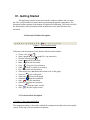
IV - Getting Started....................................................................................................... 54
4.1 Horizontal Toolbar Description .......................................................................... 54
4.2 Vertical toolbar description................................................................................. 54
V - FEATURES ............................................................................................................ 56
5.1 Change component properties............................................................................. 56
5.2 Name a component ............................................................................................. 56
5.3 Station view ....................................................................................................... 56
5.4 Create/Insert Library ........................................................................................... 57
5.5 Save/Open ........................................................................................................... 57
5.6 Cut/paste/copy..................................................................................................... 58
5.7 Remove ............................................................................................................... 58
5.8 Zoom ................................................................................................................... 58
5.9 Optimize.............................................................................................................. 58
5.10 Simulate ............................................................................................................ 58
5.11 View simulation data ........................................................................................ 59
5.12 Replay ............................................................................................................... 59
5.13 Bend pipes......................................................................................................... 59
VI – FAQ ...................................................................................................................... 59
CHAPTER 13: Technical Manual .................................................................................... 61
I- Purpose ...................................................................................................................... 61
II - Description .............................................................................................................. 61
2.1 Adding and modifying components .................................................................... 61
2.2 Mouse click handling and popup menu .............................................................. 68
2.3 Mapping cells and jobComponents..................................................................... 68
III- Naming Conventions .............................................................................................. 68
3.1 File names ........................................................................................................... 69
3.2 Variable names.................................................................................................... 69
IV- Communications..................................................................................................... 69
4.1 GUI-Optimizer .................................................................................................... 70
4.2 GUI-Simulator .................................................................................................... 70
V- Java Web Start ......................................................................................................... 70
References:........................................................................................................................ 72
Acknowledgements: .......................................................................................................... 73
CHAPTER 1: PROJECT OVERVIEW
1. Purpose
The purpose of this project is to develop a virtual pipeline simulation testbed. The
simulation will model the pressure and flow rate distribution of gas in a real pipeline
system.
2. Goals
The design and implementation goals are:
• Design a GUI to create and manipulate the pipeline system.
• Implement an optimizer to efficiently distribute computation among several
machines.
• Integrate the GUI with a simulator that will simulate the behavior of each
component of the real pipeline system by solving a set of particular partial
differential equations.
3. Constraints
When developing a simulation, the main constraint is the time. The simulation has to run
in a reasonable amount of time. For this reason, the software will use various parallel and
distributed algorithms. Another constraint is the space constraint (memory). The project
will take into consideration those constraints and will be designed to optimize the use of
time and space.
CHAPTER 2: Software Requirement Specification
1. Introduction
1.1Purpose
The purpose of this Software Requirement Specification is to establish and maintain a
common understanding between the customer, Dr. Wallentine, and the software
developer regarding the requirements for the proposed software.
1.2 Scope
The proposed software is a GUI and a job distribution optimizer for a virtual pipeline
simulation testbed. The software will simulate the pressure and flow distribution that is
happening in a real pipeline system. The software will use various parallel algorithms on
several machines in order to reduce the amount of time needed by this computingextensive simulation. The software will also provide a GUI to graphically build the
pipeline system and will perform the require computation in order to have a simulation as
accurate as possible in a reasonable amount of time. The GUI will also be used to
visualize the result of the simulation.
1.3 Overview
This Software Requirements Specification (SRS) is organized into two main sections:
overall description and specific requirements. The overall description section provides
information describing general factors that will affect the requirements of the software.
The specific requirements section describes in detail the requirements the software must
meet.
2. Overall description
2.1 Product perspective
The software is an interface to the Virtual Pipeline Simulation Testbed. It comprises a
GUI (Pipeline Editor) and a job distribution optimizer (Optimizer). Once the pipeline
system is drawn, the optimization and the simulation will be able start. The computation
will be done on several powerful computers and result will be transmitted back to the
GUI for display. Communication among cluster machines will be done by message
passing and shared memory.
2.2 User interface: Pipeline Editor
a) The pipeline editor shall support drag and drop operations for drawing
components (pipes, joints, and compressors).
b) The pipeline editor shall support standard editing functions (copy, cut,
paste).
c) The pipeline editor shall provide zoom functions.
d) The pipeline editor shall display the simulation results.
e) The user shall be able to store/retrieve a previously drawn pipeline system
(group of components called library) and connect it with some new groups
or components.
f) The user shall be able to move components inside the editor to have a
better positioning.
g) The user shall be able to edit the characteristic of each component
displayed.
h) The user shall be able to define some checkpoints during the simulation.
i) The user shall be able to playback (replay) the simulation from any given
checkpoints.
j) The user shall be able to start the application from any machines (using a
browser and WebStart).
k) At any time during the simulation, the user shall be able to interrupt the
simulation.
2.3 Hardware interfaces
a) Each computer shall have enough memory and enough computing power
(processors) to handle computing-extensive tasks.
b) Each computer shall have an Ethernet card to communicate with other
computers.
2.4 Software interfaces
a) The cluster computers shall run under the Linux operating system.
b) Each computer shall have the Java Virtual Machine installed (version 1.4
or later).
c) Each computer shall have the JGraph 3.0 package installed.
2.5 Communications interfaces
Computers shall support TCP/IP to communicate with each other.
2.6 Product functions
a) The product shall provide a GUI with all the components needed to draw a
complete pipeline system, a button to start the optimizer and a button to start the
simulation.
b) The product shall provide an optimizer. The optimizer should be able to produce a
job allocation that balances the load of each processor (that is, minimizes the load
differences among cluster machines assigned to the simulation). The jobs are the
pipelines components (pipes, joints, compressors …). Each job has some
computation time and some communication time. The computation time depends
on the characteristic of the component and the machine on which it is executed.
The communication time depends on the amount of information exchanged and
whether or not the connected component are on the same machine (local
communication) or not (remote communication). Given these constraints, the
optimizer will find an optimal distribution of jobs among machines that
minimizes the workload of each processor.
c) The product shall integrate a simulator. The simulator should solve a set of partial
differential equations that mathematically models the pressure and flow rate
distribution in each component of the real pipeline system.
2.7
User characteristics
a) Users of the system should be experienced pipeline design engineers who
have a good understanding of a pipeline system.
b) Users should be able to understand and manipulate pipeline
characteristics.
c) No particular training should be necessary to use the software.
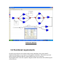
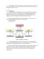
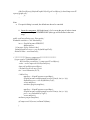
Following is the use case diagram for the software:
Save/Open Library
Save/Open Network
Draw/Edit Network
Replay
Optimize
User
Insert/Delete Checkpoint
Start Simulation
Interrupt Simulation
Virtual Pipeline Simulation System: Use Case
3. Specific requirements
3.1 External interface requirements
The interface provided will be the pipeline editor. It should be able to be started from
any computer via a browser using Java WebStart. The interface should provide all the
necessary components to draw a complete pipeline system. Characteristics of those
components shall be defined at the time of their creation. As the pipeline system can be
very large, the interface shall provide a way to save/retrieve previously built pipeline
subsystems. The interface will consist of one window with 2 toolbars and one menu bar.
The horizontal toolbar will have a button for the components and will support drag and
drop to insert components. The vertical toolbar will contain all the buttons for editing and
zooming. The menu bar will offer the same functionality as the 2 toolbars in addition of
the save/open function. The interface will offer the possibility to use the keyboard via
some shortcut keys.
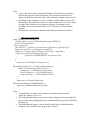
Following is a screenshot of a prototype GUI:
PIPELINE EDITOR
3.2 Functional requirements
In order to provide the most realistic and accurate simulation, the system should
implement adequately every features of the pipeline simulation. Each feature presents
some required conditions that the system should meet to react correctly.
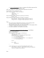
The diagrams below show the sequence diagram and the interaction of the different parts
of the software.
Client Side
: User
Server Side
---Socket---
: Pipeline Editor
: Server
: Optimizer
: Simulator
Click link in Browser
Download Application (WebStart)
Drag component
Display component
Build Network
Display Network
Save Network
Optimize ()
Optimize (Graph)
BuildJobGraph(graph)
Optimize(JobGraph)
WriteFile(jobsLists)
Simulate()
Simulate(JobsFilename)
ReadFile(filename)
Simulate
Display Data
Interupt
Send simulationData
Interupt
Stop Simulation
Interupt_confirm
End of simulation
End of simulation
End of simulation
End_confirm
replay
ReadFile
Send Replay Data
Sequence diagram of the Virtual Pipeline Simulation Testbed
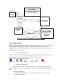
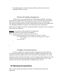
**Graph Model ,
**Component Characteristics (
Type, Diameter, Length, Index,
Value, Gas-Type )
User Input
PIPELINE
EDITOR
OPTIMIZER
Simulation
Data
SIMULATOR
** List of Job Objects
(JobTypt, Machine,
Connections, File,
Parameters,
ExecTime)
Dataflow of the Virtual Pipeline Simulation Testbed
3.2.1 Pipeline Editor
Inputs: The input for the pipeline editor should come from the user. The user will define
the components belonging to the pipeline system along with their characteristics.
Outputs: The pipeline editor shall produce a list of component objects. A component can
be either a pipe or a compressor.
a. List of components
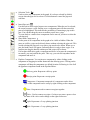
The GUI shall provide the following components: pipes, station, split, joint, orifice meter,
storage, compressor, driver, regulator, receipt point, delivery point.
Following are the icons used in the GUI:
Compressor
Pipe
Split
Station
Storage Orifice
Receipt
b. Draw a component
The user shall be able to draw any components needed for the pipeline system
either by clicking on the component icon in the toolbar or by dragging it into the drawing
pad.
a) Draw a compressor
A compressor shall only be connected to pipelines. It can accept several
pipelines connections.
b) Draw a joint
A joint should be connected to at least two pipelines. Pipelines should be the
only components connectable to joints.
c) Draw a pipe
Pipes should have another component connected at each end.
c. Delete a component
The user shall be able to delete any components in the pipeline system either by
right-clicking on the component and selecting remove or by clicking on the remove icon
in the toolbar or using the delete key.
d. Edit a component
The user shall be able to edit the characteristics of any components inside the
pipeline system by using the right-click menu. Features available for editing should
depend on the component selected.
e. Move a component
The user shall be able to move any components of the pipeline system inside the
drawing space using a dragging move. All the components connected to the component
moved should also move and stay connected.
f. Undo/Redo an action
The user shall be able to undo or redo any action done on any components of the
pipeline system either by clicking on an icon in the toolbar. If there is no action to undo
(or redo), the button should be disable.
g. Copy/Cut/Paste a component
The user shall be able to copy, cut or paste any components of the pipeline system
using the buttons in the toolbar or the standard keyboard shortcuts.
h. Zoom in/Zoom out
The user shall be able to zoom in or zoom out any area of the pipeline system
using the buttons in the toolbar.
i. Optimize
The user shall be able to launch the optimizer from the GUI by clicking on a
button on the toolbar.
j. Simulate
The user shall be able to launch the simulation from the GUI by clicking on a
button on the toolbar.
k. Insert a checkpoint
The user shall be able to launch insert a checkpoint at any time during the
simulation.
l. Playback
The user shall be able to restart the simulation by providing a checkpoint from
where the simulation should be restarted.
3.2.2 Optimizer
Input: A list of components objects
Output: A list of job objects. In addition to the fields of a component, a job has
information about the machine on which it should be executed, the components
connected to it, the execution time and the associated file containing the source code of
its execution.
The job allocation optimization is a discrete optimization problem. The system
will use the Branch and Bound algorithm to find the best distribution given some time
and communication constraints. The solution may not be optimal but should be very close
to the optimal one. The optimizer should adequately balance computation and
communication time among all the processors. It should output a list of all jobs along
with the machines on which they should be executed in order to have the best
distribution.
3.2.3 Simulator
Input: A list of job objects
Output: A list of job object with their new property values.
The simulator should solve a set of partial differential equations to simulate the
pressure and flow rate distribution in each component of the pipeline system. It should
continuously output some values in order to visualize the current state of the simulation
in the GUI.
3.3. Performance requirements
The system should be able to handle at least a set of 1000 jobs. The computation time
should be kept minimal in both the optimizer and the simulator. The user should not wait
more than 20 minutes to have the output of the optimizer and no more than 1 hour for the
results of the simulator. The amount of data transferred should also be kept minimal to
avoid too much communication overhead.
3.4. Software system attributes
a. Accuracy
Accuracy is the most important attribute for the virtual simulation pipeline
testbed. The simulator must accurately model the pressure and the flow in each
component of the pipeline system. If the convergence criteria are not well established, the
simulation will be far from the real model.
b. Reusability
The system will have several releases with each time an increased number of
functionality. Some new components and features will be added.
c. Maintainability
The system shall be separated into modules following the MVC (Model View
Controller) pattern. There will be a module for the GUI, one for the optimizer and
another one for the simulator.
d. Portability
The modules will be written in Java. As Java is supported on many platforms, it
should be quite easy to move to another platform. For performance reasons, some parts
will be written in some specific platform-dependant languages.
References
IEEE STD 830-1998, "IEEE Recommended Practice for Software Requirements
Specifications". 1998 Edition, IEEE, 1998.
Dr. Scott Deloach’s CIS748 lecture notes “http://www.cis.ksu.edu/~sdeloach/748”
CHAPTER 3: PROJECT PLAN
The project is divided into three phases, which are Specification phase, Design phase, and
Implementation, Testing, and Documentation phase. Each of those three phases is ended by
presentation at the end of the phase.
Project Task
Duration (Days)
Start Date
End Date
30
1
30
25
1
1
1
1
4
7/1/03
9/20/03
8/1/03
9/10/03
9/24/03
9/23/03
9/25/03
9/26/03
9/29/03
8/1/03
9/21/03
9/1/03
10/6/03
9/25/03
9/24/03
9/26/03
9/27/03
10/2/03
10/3/03
20
1
1
3
3
7
4
2
10/05/03
11/03/03
11/04/03
11/05/03
10/20/03
10/23/03
11/03/03
11/07/03
10/25/03
11/04/03
11/05/03
11/08/03
10/23/03
10/30/03
11/07/03
11/09/03
11/10/03
30
2
5
4
10
9
11/11/03
12/1/03
12/3/03
12/5/03
12/3/03
12/3/03
12/10/03
12/3/03
12/8/03
12/9/03
12/13/03
12/11/03
12/12/03
Phase I: Specification
1.
2.
3.
4.
5.
6.
7.
8.
9.
10.
Background Study (JNI, Branch & Bound)
Overview
Optimizer prototype
GUI Prototype
Software Requirements Specification
Project Plan
Cost Estimation
Software Quality Assurance Plan
Documentation for Presentation 2
Presentation 1
Phase II: Design
11.
12.
13.
14.
15.
16.
17.
18.
19.
Develop Prototype
Update SRS
Update SQAP
Test Plan
Develop Implementation Plan
Design
Formal Technical Inspection
Documentation for Presentation 2
Presentation 2
Phase III: Implementation
20.
21.
22.
23.
24.
25.
26.
Source Code
Testing and Reliability Evaluation
Create User Manual
Project Evaluation
Project Document
Documentation for Presentation 3
Presentation 3
CHAPTER 4: COST ESTIMATE
I- Function Point Analysis :
A function point analysis is a method of calculation lines of code using function points. A
function point is a rough estimate of a unit of delivered functionality of a software
project. To calculate the number of function points for a software project all the user
inputs, user outputs, user inquiries, number of files and number of external interfaces are
counted and divided into three categories: low, average and high.
• Number of user inputs
Each user input that provides distinct application oriented data to the software is
counted.
o Drag a component
o Delete a component
o Change properties of a component
o Display data of a component
o Insert a pipe
o Save/Open Graph
o Save/Load Library
o Create a station
o Remove a station
o Unfold a station
o Fold a station
o Undo/Redo action
o Copy/Cut/Paste a component
o Zoom in/Zoom out.
o Optimize
o Start Simulation
o Stop Simulation
o Start Replay
o Stop replay
•
Number of user outputs
Each user output that provides application oriented information to the user is
counted. In this context "output" refers to reports, screens, error messages, etc.
Each user input has a corresponding output. In addition some error messages can
occur:
o Bad station selection
o
o
o
o
o
•
Bad library file
Bad graph file
No optimization file
No simulation file
Graph not saved
Number of user inquiries
An inquiry is defined as an on-line input that results in the generation of some
immediate software response in the form of an on-line output. There are no
inquiries in this software.
•
Number of internal files
Each logical file generated by the program is counted. Here there are 4 types of
files:
o Graph files.
o Library files.
o Optimizer files.
o Simulator files.
• Number of external interfaces file
The external interface file is an internal logical file for another application.
o Optimizer files
o Simulator files
Each of these five major components is rated as low, average or high depending on the
number of files referenced and the number of data elements.
A score is attributed to each rating level.
External Input:
Number of data elements: 19
Number of file referenced: 2
Rating: High
Score: 6
External Output:
Number of data elements: 25
Number of file referenced: 0
Rating: Ave
Score: 5
External Inquiries:
Number of data elements: 0
Number of file referenced: 0
Rating: N/A
Score: 0
Internal files:
Number of data elements: 4
Number of user data referenced: 4
Rating: Low
Score: 7
External Files:
Number of data elements: 2
Number of user data referenced: 4
Rating: Low
Score: 5
The following table gives the formula to compute the total unadjusted function point.
Total Unadjusted Function Points: 6x6+5x5+7x15+5x10 = 216
Total Function Points = Total Unadjusted Function Points x [0.65 + 0.01 x SUM(Fi)]
where SUM(Fi) counts the technical complexity. It is generated by giving a rate on a
scale of 0 to 5 for each of the following questions. The higher the rate the more important
the function is.
Scale
1
Does the system require reliable backup and recovery?
0
2
Are data communications required?
5
3
Are there distributed processing functions?
5
4
Is performance critical?
3
5
Will the system run in an existing, heavily utilized operational
2
environment?
6
Does the system require on-line data entry?
0
7
Does the on-line data entry require the input transaction to be built over
0
multiple screens or operations?
8
Are the files updated online?
3
9
Are the input, outputs, files or inquiries complex?
4
10 Is the internal processing complex?
5
11 Is the code designed to be reusable?
2
12 Are conversions and installation included in the design?
0
13 Is the system designed for multiple installations in different
0
organizations?
14 Is the application designed to facilitate change and ease of use by the
0
user?
Total value adjustment factor
29
Total function points = 216 * [0.65 + 0.01 * 29] = 203.04
We select the language factor for applications written in JAVA to be 40.
The language factor here is an assumed value. It is expected that the language factor for
3rd generation language to lie between 20 and 60. since no code is automatically
generated by an IDE but there will be some code reused, the language factor is assumed
to be average.
Therefore the estimated source lines of code =
Total Function points * language factor = 203.04 x 40 = 8121 LOC
II- Cost Analysis Using COCOMO
The COCOMO model is a good measure for estimating the number of person-months
and the time required to develop software. The Virtual Pipeline Simulation Testbed can
be considered as an organic mode process (in-house, flexible with less-complex
development). The basic effort and schedule estimating formula is:
Effort = 3.2 EAF (Size) 1.05;
Time = 2.5 (Effort) 0.38;
Where:
Effort = number of staff-months
EAF = Effort Adjustment Factor (cf. Table)
Size = number of delivered source instructions (in thousands of lines of code)
The following table gives the value of the efforts multipliers. The product of those 15
factors will give the value of the EAF for the given project.
Cost
Driver
Description
Rating
Very
Low
Low
Nominal High
Very
High
Extra
High
Product
RELY
Required software reliability
0.75
0.88
1.00
1.15
1.40
-
DATA
Database size
-
0.94
1.00
1.08
1.16
-
CPLX
Product complexity
0.70
0.85
1.00
1.15
1.30
1.65
TIME
Execution time constraint
-
-
1.00
1.11
1.30
1.66
STOR
Main storage constraint
-
-
1.00
1.06
1.21
1.56
VIRT
Virtual machine volatility
-
0.87
1.00
1.15
1.30
-
TURN
Computer turnaround time
-
0.87
1.00
1.07
1.15
-
ACAP
Analyst capability
1.46
1.19
1.00
0.86
0.71
-
AEXP
Applications experience
1.29
1.13
1.00
0.91
0.82
-
PCAP
Programmer capability
1.42
1.17
1.00
0.86
0.70
-
VEXP
Virtual machine experience
1.21
1.10
1.00
0.90
-
-
LEXP
Language experience
1.14
1.07
1.00
0.95
-
-
Modern programming practices
1.24
1.10
1.00
0.91
0.82
-
Computer
Personnel
Project
MODP
TOOL
Software Tools
1.24
1.10
1.00
0.91
0.83
-
SCED
Development Schedule
1.23
1.08
1.00
1.04
1.10
-
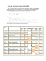
Table 2-1. Software Development Effort Multipliers (EAF)
•
EAF = 0.75 x 0.94 x 1.15 x 1.00 x 1.00 x 0.87 x 0.87 x 0.71 x 0.82 x 0.70 x 0.90 x
0.95 x 0.82 x 0.91 x 1.10 = 0.17
•
KLOC = 8 (8,000 SLOC) (Estimation)
•
E = 3.2 x 0.17 x 81.05 = 4.82 staff-month
•
Time = 2.5 x 4.820.38 = 4.54 months
Analysis:
1 staff-month = 152 hours
=> Total Time = 3326 Hours
References:
• “Software Cost Estimation: Metrics and Models”. Kim Johnson
http://sern.ucalgary.ca/courses/seng/621/W98/johnsonk/cost.htm.
• “An Introduction to Function Point Analysis”, http://www.qpmg.com/fp-intro.htm
• David Longstreet, “Fundamentals of Function Point Analysis”,
http://www.ifpug.com/fpafund.htm
CHAPTER 5: Architecture Elaboration Plan
The purpose of this document, as required by the MSE portfolio requirement, is to
define the activities and actions that must be accomplished prior to the Architecture
Presentation.
The activities and actions to be accomplished prior to the architecture presentation are
listed below:
•
Software Requirement Specification.
•
Software Quality Assurance plan
•
The Engineering Notebook
•
The vision document
•
The Cost Estimation
•
The Project plan
•
The Implementation Plan
The artifacts that will undergo formal technical inspection are:
•
Object model
•
The requirement specification
The Formal Technical Inspection will follow an IEEE standard formal checklist and will
be led by two MSE students and one student involved in the project:
1. Padmaja Havaldar
2. Sudarshan Kodwani
3. Liubo Chen
The inspectors will provide a well-documented report on the result of their inspection.
References:
http://www.cis.ksu.edu/~sdeloach/748/protected/slides/748-4-formal-inspections.pdf
CHAPTER 6: Software Quality Assurance Plan
1. Purpose
The software item covered by this SQAP is the ‘Virtual Pipeline Simulation Testbed’.
The system is used to simulate the pressure ad the flow in the components of a real
pipeline system. This SQAP covers the entire life cycle of the software.
2. Management
2.1 Organization
A committee of three professors will supervise the project. Only one developer will
implement the project. The committee consists of:
• Dr. Virgil Wallentine (Major Professor)
• Dr. Masaaki Mizuno
• Dr. Daniel Andresen.
The developer is Walamitien Oyenan.
The committee will approve the design and requirements and will be responsible for
monitoring implementation progress.
2.2 Tasks
The following tasks will be completed for the project:
• Requirements Specification
• Cost Estimation
• Project Planning
• Formal Specification & Verification
• Test Planning
• Design Documentation
• Project Presentations
• Inspections
• Implementation
• Testing & Verification
• Documentation
• Project Evaluation
2.3 Roles and Responsibilities
The developer will be responsible for all the tasks described above. He will be
under the supervision of the major professor and will report to all the committee members
in the form of three presentations.
3. Documentation
3.1 Purpose
To ensure the quality of the Virtual Pipeline Simulation Testbed, as a minimum,
the Software Quality Assurance will use the Software Design Document (SDD), the
Software Requirement Specification (SRS), the Test Plan, the Formal Specification and
the User Documentation for verifying and validating the product.
3.2 Minimum documentation requirements
3.2.1 Software requirements specification
The SRS lists the requirements of a system and it should correctly describe the
system requirements. It specifies the functionality and performance of the project in
terms of speed, reliability etc. It describes how the system interacts with the people using
it and specifies the design constraints and standards to be followed.
3.2.2 Software Test Plan
The purpose of this document will be to develop and record formal procedures for
the verification and validation of the pipeline simulation software.
3.2.3 Formal Software Specification
A section of the software will be formally specified using a formal specification
tool.
3.2.4 Software design document
This document describes the overall structure of the software. It will contain an
object model constructed using rational rose. The object model will describe the various
classes used in the project.
3.2.5 User Documentation
The user documentation will consist of a user manual, which will identify the
features of the software and their functions. It will also describe all error messages and
program limitations and constraints. The user documentation will also contain source
code.
4. Standards, practices, conventions, and metric
4.1 Purpose
This section identifies the standards, practices, conventions, and metrics to be
used in the virtual pipeline simulation system and states how the compliance will be
monitored and assured.
4.2 Content
The MSE project portfolio will serve as a guideline in developing the documents.
4.2.1 Documentation Standards
The Software Requirements Specifications (SRS) and SQA Plan (SQA) will be based
upon IEEE Software Engineering Standards.
4.2.2 Coding Standards
The source code will follow the guidelines in the Java coding standards.
4.2.3 Metrics
The COCOMO model will be used to estimate the effort and time needed for the
development of the software.
5. Reviews and Audits
5.1 Purpose
This section defines the technical and managerial reviews to be performed, and states
how they are to be accomplished.
5.2 Minimum Requirements
A number of reviews will be done during the design, development, and testing of the
project. They will be under the supervision of the committee. The following reviews
will be conducted:
• Software Requirements Review
• Preliminary Design Review
• Formal Technical Inspection
In addition, there will be three formal presentations at the end of each phase of
development as describe on the project plan.
6. Testing and Verification
To insure that the Virtual pipeline system meets the required quality, some tests have
to be performed during the development process. The system must satisfy the standard
functional requirements for the gasoline pump system stated in the SRS. The system
should also satisfy the others criteria as stated in the SRS: performance, accuracy,
reusability, maintainability and portability.
7. Problem reporting and corrective action
All problems that cannot be resolved by the developer will be reported to the major
professor. The committee will provide reviews on all current work and corrective
measures for changes will be taken. The errors and problems encountered during the
development of the project will be documented.
8. Tools, techniques, and methodologies
The project will use the JGraph3.0 library along with Swing to build the Pipeline
Editor (GUI). Rational Rose will be used to visually design the software being developed.
Alloy or OCL will be used as a formal specification tool.
References
“IEEE guide for software quality assurance planning” IEEE Std-730.1-1995
Pressman, Roger S. "Software Engineering: A Practitioner's Approach". Fifth Edition,
Mc GrawHill, NY, June, 2001.
CHAPTER 7: Architecture Design
1. System Design Description
This document contains the complete architectural design of the GUI and the
Optimizer of the Virtual Pipeline Simulation Testbed. The GUI is built as an extension of
the JGraph and Swing packages. In order to have a better understanding of the design,
this document will briefly describe the design and features of JGraph before explaining in
details the design of the GUI and the Optimizer. The complete design of JGraph can be
found online (cf. references).
There are 3 main packages in this architecture:
• Jgraph
• Editor
• Optimizer
The design of each package will be explained separately in the rest of this document.
2. JGraph design
The implementation of JGraph is entirely based on the source code of the JTree class.
However, it is not an extension of JTree; it is a modification of JTree's source code. The
components for trees and lists are mostly used to display data structures, whereas this
graph component is typically also used to modify a graph, and handle these modifications
in an application-dependent way.
2.1 - Features
The main features of JGraph are:
•
Inheritance: JTree's implementation of pluggable look and feel support and
serialization is used without changes. The UI-delegate implements the current
look and feel, and serialization is based on the Serializable interface, and
XMLEncoder and XMLDecoder classes for long-term serialization.
•
Modification: The existing implementation of in-place editing and rendering was
modified to work with multiple cell types.
Extension: JGraph's marquee selection and stepping-into groups extend JTree's
selection model.
•
•
Enhancement: JGraph is enhanced with datatransfer, attributes and history,
which are Swing standards not used in JTree.
•
Implementation: The layering, grouping, handles, cloning, zoom, ports and grid
are new features, which are standards-compliant with respect to architecture, and
coding conventions.
2.2 - The Model
The model provides the data for the graph, consisting of the cells, which may be
vertices, edges or ports, and the connectivity information, which is defined using ports
that make up an edge's source or target. This connectivity information is referred to as the
graph structure. (The geometric pattern is not considered part of this graph structure.)
Figure 1. A graph with two vertices and ports, and one edge in between
Figure 2. Representation of the graph in the DefaultGraphModel
2.3 - The View
The view in JGraph is somewhat different from other classes in Swing that carry
the term view in their names. The difference is that JGraph's view is stateful, which
means it contains information that is solely stored in the view. The GraphLayoutCache
object and the CellView instances make up the view of a graph, which has an internal
representation of the graph's model.
Figure 3. GraphLayoutCache and GraphModel
The GraphLayoutCache object holds the cell views, namely one for each cell in
the model. The graph view also has a reference to a hash table, which is used to provide a
mapping from cells to cell views.
2.4 - The control
The control defines the mapping from user events to methods of the graph- and
selection model and the view. It is implemented in a platform-dependent way in the UIdelegate, and basically deals with in-place editing, cell handling, and updating the
display. As the only object that is exchanged when the look and feel changes, the UIdelegate also specifies the look and feel specific part of the rendering.
In JGraph, the graph model, selection model and graph view may dispatch events.
The events dispatched by the model may be categorized into:
• Change notification
• History support
Figure 4. JGraph's event model
The GraphModelListener interface is used to update the view and repaint the
graph, and the UndoableEditListener interface to update the history. These listeners may
be registered or removed using the respective methods on the model.
The selection model dispatches GraphSelectionEvents to the GraphSelectionListeners
that have been registered with it, for example to update the display with the current
selection. The view's event model is based on the Observer and Observable class to
repaint the graph, and also provides undo-support, which uses the graph model's
implementation.
3. Pipeline Editor Design
Most of the classes of the Pipeline Editor extend the classes of JGraph in order to
provide a custom graph needed to draw the pipeline network. Only a few classes directly
extend some Swing classes. The features implemented by the pipeline editor are
described in the Software Requirement Specification document.
3.1 - Class diagram
Following is the class diagram of the pipeline editor:
Mediator
graph : MyGraph
optimizer : optimizerClient
simulator : SimulatorClient
DefaultGraphModel
optimize()
simulate()
stopSimulation()
Replay()
updateData()
Editor
optimizer
graph
graphUndoManager
SimulatorClient
OptimizerClient
run()
isDone()
setCommand()
getCommand()
setFilename()
getStatus()
setStatus()
run()
isDone()
setFilename()
setTime()
setJobs()
ungroup()
group()
isGroup()
undo()
redo()
property()
open()
save()
openLib()
saveLib()
valueChanged()
keyPressed()
createMenuBar()
createToolbar()
ButtonTransferHandler
type : String
getType()
createTransferable()
getSourceActions()
GraphTransferHandler
JGraph
MyModel
PortView
MarqueeHandler
MyPortView
portIcon : ImageIcon
acceptSource()
acceptTarget()
getBound()
getRenderer()
MyGraph
selectPipe : boolean
actionMap : ActionMap
MyMarqueeHandler
graph : MyGraph
connect()
isForceMarqueeEvent()
mousePressed()
mouseDragged()
mouseReleased()
getSourceportAt()
getTargetPortAt()
mouseMoved()
createPopupMenu()
getAction()
isCellEditable()
insert()
createVertexView()
createPortView()
createEdgeView()
getArchivableState()
setArchivableState()
DefaultGraphCell
MyGraphTransferHandler
MyCell
dataCell : DataCell
importDataImpl()
doImport()
getDataCell()
setDataCell()
CompressorCell
DataCell
VertexRenderer
DataRenderer
dataPanel : JPanel
getRendererComponent()
installAttributes()
JointCell
pipeCell
MyUserObject
properties : Map
CompressorView
JointView
PipeView
paint()
paint()
paint()
valueChanged()
getProperty()
setProperty()
getProperties()
setProperties()
clone()
showPropertyDialog()
VertexView
Figure 5: Class Diagram of the Pipeline Editor
3.2 - Class description
This section describes each class of the pipeline editor and its function. For the
classes extending JGraph classes, only the purpose of the extension is explained. To
understand the whole function of the class, it is necessary to refer to the extended class in
the JGraph package.
Class Editor extends JPanel:
This is the main class representing the main panel of the application. It has the graph
panel (instance of JGraph) and the toolbars.
Class MyGraph extends JGraph:
Provide a custom graph model.
Contains all the necessary methods to create and insert custom components in the graph.
Class MyMarqueeTransferHandler extends MarqueeTransferHander:
Provide a custom mouse handler for the graph.
Provide custom edges used to represent pipes.
Create popup dialogs.
Class MyModel extends GraphModel:
Define the criteria to accept the connection edge (pipe) and cell (component)
Class MyPortView extends Port view:
Define a custom representation of ports.
Class MyGraphTransferHandler extends GraphTransferHandler:
Provide drag and drop support for the graph.
Class ButtonTransferHandler extends TransferHandler:
Transfer Handler for dragging the buttons from the toolbar.
Class DataCell extends DefaultGraphCell:
Define a cell use to display data from the simulation.
This cell is a JPanel.
Class DataRenderer extends VertexRenderer:
Use to render the DataCell as a JPanel containing information to be displayed.
Class MyCell extends DefaultGraphCell:
Abstract class for all the custom cells representing the components.
Each MyCell object has a reference to a DataCell.
Class CompressorCell extends MyCell:
Represent a component cell. The component is a compressor.
Each component cell has a DataCell and a MyUserObject to holds information about the
cell.
There is similar class for each component (Pipe, Joint, Split …).
Class CompressorView extends VertexView:
Define the shape of the component.
There is similar class for each component (Pipe, Joint, Split …).
Class MyUserObject extends Object:
Holds the property of the associated object (component) in a map for future reference.
Display the property dialog for each component.
Class SaveServer:
Server to save the user file on the server side.
Receive the file via socket and save it.
Class SaveClient:
Send the file to be saved to the server via socket.
Class Optimizer:
Create JobComponent objects from component cells taken from the graph.
Each component cell has a corresponding JobCcomponent.
Holds a reference to BranchBound class to start the optimization.
4. Optimizer Design
Problem: Given a set of jobs with execution time and computation time and a set of
machines, find the optimal job distribution among those machines. That is, find the
distribution that minimizes the differences in the load of each machine.
4.1 - Depth-First Branch and Bound
Each job j has a computation weight Wj and a communication time Cj (sum of
each communication time with all neighbors).
The objective is to minimize the load on the busiest machine.
At each node, we consider a cost function for the busiest machine only (worst-case
estimate).
A vertex in the tree represents a partial/complete allocation of jobs on machines.
The root of the search tree is the empty allocation.
A vertex at level k in the tree represents an assignment of jobs {J1,…,Jk}.
a) Cost function
The cost function f(x) is defined by:
f(x) = g(x) + h(x) ;
where:
g(x) : actual cost for the current allocation.
h(x) : load contribution on the busiest machine of the next job to be allocated.
We have:
•
g(x) = ∑(Wj+Cj) for all j allocated to the busiest machine.
Note: Cj consider only the communication with neighbors already allocated.
• h(x) = min(Wi, Ci) , i being the next job to be allocated.
The heuristic function h(x) is explained as follows:
*If job i is eventually assigned on the busiest machine, its contribution to this
node’s load is just its weight.
*If job i is eventually allocated on some other machine, its contribution to the
node’s load is its communication time.
At each step, we want the take the case that minimize h(x).
b) Pseudo Algorithm:
minCost = infinity,
root = empty allocation,
cost(root) = 0
stack = allJobs
While stack not empty do
node = dequeue stack
if node isLeaf, update minCost
else
compute cost(node)
if cost(node) > minCost then prune node
else generate job allocation of all children of node
end if
end if
end while
return minCost
The following figure shows an execution of the Branch and Bound algorithm with
3 tasks (T1, T2, T3) and 2 processors (N1, N2) without and with pruning (Fig 7, 8).
Fig. 6: Example with 3 tasks(T1, T2, T3) and 2 processors (N1, N2) without pruning
Figure 7: Example with 3 tasks (T1, T2, T3) and 2 processors (N1, N2) with pruning
c) Shared Version
In the shared version, the sequential algorithm is started. When there are enough nodes,
the nodes are distributed among workers. Each worker can the start its own branch and
bound algorithm. Every time a new bound is reached, it is compared to the shared bound
and updated if necessary. At the end, the shared bound, which is the minimal found, will
be associated to a solution object (containing the minimal allocation). This solution
Object will be returned.
4.2 - Class Diagram
SharedBound
value : float
solution : Solution
BranchBound
minCost : Solution
active : Stack
node : Node
Solution
value : int
allocation : Vector
getValue()
getAllocation()
getValue()
setValue()
getSolution()
setSolution()
findSolution()
startSolution()
Optimizer
graph : JGraph
workers : Vector
allJobs : Vector
allMachines : Vector
Worker
solution : Solution
stack : Vector
numMachine : int
numJobs : int
optimize()
createPipe()
createJoint()
createCompressor()
addNode()
CompareJob
compare()
Node
allocated : Vector
remaining : Vector
allocation : Vector
load : Vector
leaf : boolean
getLoad()
getCost()
setLoad()
setCost()
setAllocation()
getAllocation()
isLeaf()
getLoadForMachine()
setLoadForMachine()
getAllocationForMachine()
JobComponent
machineID : int
componentType : int
componentID : int
neighborsIn : Vector
neighborsOut : Vector
Machine
numProcessors : int
name : String
id : int
speed : int
getMachineId()
getcomponentType()
getComponentId()
getNeighborsIn()
getNeighborsOut()
Pipe
diameter (0.6m) : double
length (100000.0m) : double
theta (0.0) : double
nodes (51) : int
gasType (1) : int
hin (200.0) : double
tin (298.15) : double
p_1 : double
p_nodes : double
number (3) : int
index : int[3]
value : double[3]
p : double[51]
t : double[51]
m : double[51]
Joint
Compressor
gasType (1) : int
ps : double
ts : double
ms : double
pd : double
td : double
md : double
power (1000.0) : double
speed (14000.0 : double
efficiency (75.0) : double
head (20.0) : double
fuel (1.0) : double
number(4) : int
index : int[4]
value : double[4]
Figure 9: Class Diagram of the Optimizer
getPower()
getNumProcessor()
getSpeed()
4.3 - Class Description
Class BranchBound
Implement the branch and bound algorithm.
Holds a reference to the current solution found.
Class Solution
Represent a solution to the Branch and Bound algorithm.
Contains the minimal allocation found.
Class Node
Holds the current allocation. The allocation can be partial (non-leaf node) or complete
(leaf node).
For a non leaf node, jobs non allocated yet are stored inside the node.
An allocation is an array of machine with their corresponding jobs.
Class Machine
Holds all the information about a machine.
Store all the jobs allocated to this machine so far.
Class JobComponent
Abstract class representing a job. Sub classes of this class are component objects (pipe,
compressor, joint…) .
Class Pipe extend JobComponent
Holds all the properties and initial values of a pipe.
There is a similar class for all components (Compressor, Joint, split…).
Class Worker extends Thread
Worker objects are threads searching a part of the tree.
They exchange new bounds via a shared memory (class SharedBound).
Holds a stack of nodes representing their part of the tree.
Class SharedBound
Holds the minimal bound found so far by the Worker objects.
Also holds the allocation (Solution object) corresponding to this bound.
Class CompareJob
Used to specify how jobs should be compared.
When the jobs are sorted, it helps reducing the number of nodes visited to reach the
solution.
Jobs are compared by number of neighbors and by weight.
References:
• Gaudenz Alder, Design and Implementation of the JGraph Swing Component
http://www.jgraph.com/documentation.shtml
•
Dar-Tzen et al., Assignement and Scheduling Communicating Periodic Tasks in
Distributed Real-Time Systems, IEEE Transactions on Parallel and Distributed
Systems, 1997
CHAPTER 8: Formal Requirement Specification
Introduction
This document specifies the protocol between the GUI on the client side and the
simulator on the server side.
Specification
The GUI needs to be able to listen to the simulator in order to get the data from the
simulation. When the user wants to start a simulation, he needs to pass a filename to the
simulator. If this filename is not valid, an error code is returned. If it is a valid filename
(the file exists and has the proper format), then the GUI is ready to accept data from the
server. As long as there is some data available, the server continues to send them. At any
time, the user can interrupt the simulation. A message is then sent to the simulator. The
protocol will make sure that there is no loss of data due to interruption. The server can
also send an end message when the simulation reaches the end. At the end (either by
interruption, or normal termination), both the server and the GUI should be ready to start
the protocol again.
Verification
The protocol is specified using Promela and checked with Spin. We want to check
that the protocol has no deadlock. We also want to be able to verify that there are no
unexpected messages. (E.g. a data message when expecting an end message).
Following are the FSMs used to derive the Spin Model:
Send file
init
wait
Recv reject
Send done
Recv accept
Recv done
Recv_
done
Recv done
data_ex
Send_
done
Send done
Recv data
Recv data
Figure 1: FSM for the GUI
Figure 2: FSM for the Simulator
SPIN Model:
/* Protocol GUI - Simulator
* Virtual Pipeline Simulation Testbed
*
* Walamitien OYENAN
*/
#define idle 0
#define wait 1
#define check 2
#define data_ex 3
#define recv_done 4
#define send_done 5
#define MAX 4
int datasent = 0;
mtype = {file, reject, accept, data, done}
chan socket1 = [MAX] of {mtype}
chan socket2 = [MAX] of {mtype}
proctype gui (chan send, recv) {
int state = idle;
end:
do
:: atomic { state == idle ->
send ! file;
state = wait;
}
:: atomic { recv ? reject ->
assert (state == wait);
state = idle
}
:: atomic { recv ? accept ->
assert (state == wait);
state = data_ex;
}
:: atomic { recv ? data ->
assert (state == data_ex || state == send_done);
skip;
}
:: atomic { recv ? done ->
assert (state == data_ex || state == send_done);
if
:: state == data_ex ->
state = recv_done;
:: state == send_done ->
state = idle;
fi
}
:: atomic { state == data_ex ->
send ! done;
state = send_done;
}
:: atomic { state == recv_done ->
send ! done;
state = idle;
}
od
}
proctype simulator(chan send, recv)
{
int state = idle;
end:
do
:: atomic { state == idle ->
recv ? file;
state = check;
}
:: atomic { state == check ->
send ! reject;
state = idle
}
:: atomic { state == check ->
send ! accept;
state = data_ex;
}
:: atomic { recv ? done ->
assert (state == data_ex || state == send_done);
if
:: state == data_ex ->
state = recv_done;
:: state == send_done ->
state = idle;
fi
}
:: atomic { state == data_ex ->
if
:: datasent < MAX ->
send ! data;
datasent++
:: else ->
send ! done;
state = send_done;
fi
}
:: atomic { state == recv_done ->
send ! done;
state = idle;
}
od
}
init {
atomic {
run gui(socket1,socket2);
run simulator(socket2, socket1);
}
}
SPIN Output:
(Spin Version 3.4.16 -- 2 June 2002)
+ Partial Order Reduction
Full statespace search for:
never-claim
assertion violations
cycle checks
- (not selected)
+
- (disabled by -DSAFETY)
invalid endstates
+
State-vector 56 byte, depth reached 53, errors: 0
162 states, stored
152 states, matched
314 transitions (= stored+matched)
330 atomic steps
hash conflicts: 0 (resolved)
(max size 2^19 states)
2.542 memory usage (Mbyte)
Reference:
“Spin Online References”, http://spinroot.com/spin/Man/index.html
CHAPTER 9: Test Plan
1. Introduction
The Software Test Plan (STP) describes the plans for testing the software. The
purpose of the test plan is to ensure that the intended functionalities are implemented
properly. To fulfill this objective, a series of test will be executed during the
implementation.
2. Scope
This plan will address only those items and elements that are related to the GUI and
the Optimizer of the Virtual pipeline Simulation Testbed. The primary focus of this plan
is to ensure that the GUI provides the appropriate functionalities and that the optimizer
produces an optimal solution.
The project will have three levels of testing, Unit, System/Integration and Acceptance.
Unit testing focuses verification effort on the major functions, and integration testing
tests the program structures built with unit-tested modules. The details for each level are
address in the approach section and will be further defined in the level specific plans.
3. Test Item
These are the items to be tested:
• Pipeline Editor
• Optimizer
4. Features to be Tested
•
•
•
•
Pipeline Editor functions
Optimizer performance
Communication GUI – Optimizer
Communication GUI - Simulator
5. Approach
5.1. Unit Testing
There will be mainly two units: the GUI unit and the Optimizer unit. All the
classes will be tested in the unit they refer to. Classes belonging to both units
(JobComponent and subclasses) will be tested only in the GUI unit.
5.2. Integration testing
Once the individual units have passed unit testing those units may then be used in
integration testing. During integration testing, the units will be incorporated together
and tested, adding one unit at a time. Integration testing will put together the GUI
unit and the Optimizer unit.
6. Test Cases
6.1. Unit Tests
Pipeline Editor–
• Given a network, all operations as define in the Software Requirement
Specification should produce the expected result.
• Drawing a network should meet all the requirements as defined in the
Software Requirement Specification document.
Optimizer –
• Given a set of jobs and machines, it should produce the correct output.
• Will have the capability to produce an optimal solution with at least
1000 jobs.
6.2. Integration Tests
GUI-Optimizer: Given a network, the GUI and the Optimizer should be able to
communicate effectively and produce the expected file as output.
7. Pass/Fail Criteria
The system will pass if the functionality and performance requirements are met.
6. Suspension Criteria
Suspension Criteria: If any of the tests selected by the member do not give the expected
result, then the testing will be suspended until the bug is fixed.
8. Deliverables
•
•
•
Test Plan.
Test Case Specification.
Test input and test output data.
9. Responsibilities
The developer is responsible for all the testing activities.
10.
Schedule
Unit Testing – each unit will be tested during implementation.
Integration Testing – as the program units are integrated together, the program
will be tested.
11.
Approval
Approved by Committee Members.
Reference:
“IEEE Standard for Software Test Documentation”, IEEE Std 829-1998
CHAPTER 10: Implementation Plan
The Implementation plan will define the tasks to be completed during
implementation. The tasks are as following:
User Manual
The Manual will describe all the features of the software (Pipeline Editor and Optimizer).
It will also describe in detail how to use the pipeline editor. The completion criteria for
this task would be when all the features and their use have been successfully described.
Architecture Design
The architecture design will be revised every time a change occurs. These changes will
be documented along with the component design.
Source Code
The source code will be documented using the javadoc documentation. This source code
will comply with the architecture design.
Assessment Evaluation
This assessment evaluation will contain a report of the tests done on the software and the
results of these tests in the form of a test log.
Project evaluation:
The project evaluation document will review the process adopted for the implementation
of this project and the effectiveness of the methodologies used. The completed software
will be reviewed to check if it complies with the initial overview of the project. The
product will also be reviewed to check the quality of the product.
The implementation of the software will be considered completed when
•
•
•
The critical functions of the GUI will be implemented
The optimizer will successfully compute the optimal distribution
The GUI will successfully display the result of the simulation
Other documents:
Formal Technical Inspection reports.
CHAPTER 11: Formal Technical Inspection
Introduction
This document provides a formal checklist for the requirement specification
document of the software. The purpose of this document is to ensure the quality of the
software requirements. The checklist will be evaluated by three students and their report
will be documented.
Items to be inspected
The Software Requirements Specification document (version 2.0) will be inspected.
Participants
•
•
•
Padmaja Havaldar
Sudershan Kodwani
Liubo Chen
Criteria
Input: The Inspectors should review the SRS document and evaluate if Yes/No/Partial
and suggest comments if needed.
Output: The inspectors’ reports.
Formal Technical Inspection Check List
Compatibility
•
Do the interface requirements enable compatibility of external interfaces
(hardware and software)?
Completeness
•
•
•
•
•
•
Does SRS include all user requirements (as defined in the concept phase)?
Do the functional requirements cover all abnormal situations?
Have the temporal aspects of all functions been considered?
Does SRS define those requirements for which future changes are anticipated?
Are all normal environmental variables included?
Are the environmental conditions specified for all operating modes (e.g., normal,
abnormal, disturbed)?
Consistency
•
•
Is there any internal inconsistency between the software requirements?
Is the SRS free of contradictions?
•
•
•
•
Does SRS use standard terminology and definitions throughout?
Is SRS compatible with the operational environment of the hardware and
software?
Has the impact on the environment on the software been specified?
Has the impact of software on the system and environment been specified?
Correctness
•
•
•
•
•
•
Does the SRS conform to SRS standards?
Are algorithms and regulations supported by scientific or other appropriate
literature?
Does SRS reference desired development standards?
Does the SRS identify external interfaces in terms of input and output
mathematical variables?
What is the rationale for each requirement? Is it adequate?
Is there justification for the design/implementation constraints?
Feasibility
•
•
Will the design, operation, and maintenance of software be feasible?
Are the specified models, numerical techniques, and algorithms appropriate for
the problem to be solved?
Modifiability
•
•
•
Are requirements organized so as to allow for modifications (e.g., with adequate
structure and cross referencing)?
Is each unique requirement defined more than once? Are there any redundant
statements?
Is there a set of rules for maintaining the SRS for the rest of the software
lifecycle?
Traceability
•
Is there traceability from the next higher level spec (e.g., system
concept/requirements and user needs as defined in concept phase, and system
design)?
•
•
Does the SRS show explicitly complete coverage of requirements defined by client?
Is SRS traceable forward through successive development phases (e.g., into the
design, code, and test documentation)?
Understandability
•
•
Does every requirement have only one interpretation?
Are the functional requirements in modular form with each function explicitly
identified?
•
•
•
•
•
•
Is there a glossary of terms?
Is formal or semiformal language used?
Is the language ambiguous?
Does the SRS contain only necessary implementation details and no unnecessary
details? Is it over specified?
Are the requirements clear and specific enough to be the basis for detailed design
specs and functional test cases?
Does the SRS differentiate between program requirements and other information
provided?
Maintainability
•
•
Does the documentation follow MSE portfolio standard
Is the documentation clear and unambiguous
Verifiability/Testability
•
•
Are the requirements verifiable (i.e., can the software be checked to see whether
requirements have been fulfilled)?
Is there a verification procedure defined for each requirement in the SRS?
Clarity
•
•
•
•
Are all of the decisions, dependencies, and assumptions for this design
documented?
Are names indicative of their meaning?
Is each concept defined only once, with one clear meaning?
Is each statement written as clearly as possible?
Functionality
•
Does the design implement the specification and requirements?
Reliability
•
•
Are abnormal conditions considered?
Are the defect conditions/codes/messages specified completely and meaningfully?
References
IEEE Std 1028-1998, “IEEE Standard for Software Reviews and Audits”. 1998 Edition, IEEE, 1983.
“Software Formal Inspections”, Software
http://satc.gsfc.nasa.gov/fi/fipage.html
Assurance
Technology
Center
(SATC),
1997,
Weiss, Alan R. and Kerry Kimbrough, “Fundamentals of Software Inspections, Version 2.1”. 1995.
http://www2.ics.hawaii.edu/~johnson/FTR/Weiss/weiss-intro
CHAPTER 12: USER MANUAL
I - System Overview
The Pipeline Editor is a feature-rich graphical user interface designed to provide
pipeline designers with a graphical view of their pipeline systems and simulation data.
This allows for quick pipeline design and data generation. The software integrates an
optimizer, which goal is to optimize the time of the simulation. As the simulation is done
among several distributed machines, the optimizer will attribute each component of the
pipeline system to a particular machine in order to minimize the overall time needed to
compute the simulation data. The Pipeline Editor can be started from any computers.
Once started, it will connect to the optimizer and the simulator server.
II - System Requirements
•
•
•
The execution of the software requires Java Web Start 1.2. It is a tool that allows
user to access the application from any computer using an Internet browser.
The user should also have access to the C drive in order to write some data in the
temporary folder.
To start the application, Netscape Navigator or Internet Explorer (or any other
browser) is needed. For the first time, an internet connection is needed. After the
application has been downloaded, the user will have the choice to integrate the
application in the desktop in order to be able to run it offline.
III - Installation and Execution
No particular installation steps are needed. In case the computer does not have
Java web Start installed, it will needed to be installed. Visit
http://java.sun.com/products/javawebstart/download.html to install the latest version of
Java Web Start.
To execute the software, go to
http://www.cis.ksu.edu/~oyenan/MyWeb/project/project.htm and click on Pipeline Editor
or directly point your browser to this address:
http://www.cis.ksu.edu/~oyenan/MyWeb/project/project.jnlp. The application should start
downloading. A security-warning window will appear. Accept to launch the application.
The application will then start.
IV - Getting Started
The application consists of one main window with two toolbars and one menu
bar. The vertical toolbar has some buttons representing the pipeline components. The
horizontal toolbar contains all the buttons for editing and simulating. The menu bar offers
the functionality of the horizontal toolbar in addition to some other functions later
described.
4.1 Horizontal Toolbar Description
Figure 1: The horizontal toolbar
Following is the description of each button of the horizontal toolbar:
• Create a new graph ( )
• Open a graph: ( ) Open a graph file (.vps extension)
• Save the current graph ( )
• Undo : ( )undo the last action
• Redo: ( )Redo the last action
• Copy: ( ) Copy the selected item(s)
• Paste : ( ) Paste a copied or cut item(s)
• Cut : ( )Cut the selected item(s)
• Zoom actual size: ( ) Return the normal scale of the graph
• Zoom in: ( )Zoom in the graph
• Zoom out: ( )Zoom out the graph
• Simulate: ( ) Start the simulation
• Stop : ( ) Stop the simulation
• Optimize: ( ) Start the optimizer
• Replay: ( ) Start the replay session
• Stop : ( ) Stop the replay session
4.2 Vertical toolbar description
<= Figure 2: The component toolbar
The component toolbar is the toolbar with all the components needed to draw the pipeline
system. Following is the description of its buttons:
•
Selection Tool: ( )
Used to select any components in the graph. It is always selected by default
except when the pipe tool is selected. Use this button to cancel the pipe tool
selection.
•
Insert Pipe tool:
Use this tool to insert a pipe between two components. When the tool is selected,
the cursor becomes a cross. Rolling over a component port will then cause this
port to be highlighted. This indicates the possibility of connecting a pipe to this
port. You can then drag the cursor to another port to have a pipe.
To come back to a mode where components can be moved, you have to select the
selection tool.
Show/Hide Connectors:
Set the ports of all components in the graph to be visible or hidden. When the
ports are visible, a pipe can be directly drawn without selecting the pipe tool. This
avoids selecting the pipe tool every time a pipe needs to be drawn. When over a
port, the hand cursor will appear, indicating that it is ready to draw a pipe. You
can then just drag the hand to another port and a pipe will be drawn.
If it becomes difficult to grab a component and move it (because the component is
too small), you can just hide the ports. This way, you can click anywhere on the
component and move it.
•
•
Pipeline Components: You can insert a component by either clicking on the
component or dragging its toolbar button into the drawing space. Clicking on the
component will drop the component at a default location. Following is a list of all
the pipelines component found in the Pipeline Editor:
Delivery point: Represent a delivery point.
Receipt point: Represent a receipt point.
Compressor: Component composed of a compressor and a driver.
Type of this component can be set up by right-clicking on the component.
Joint: Component used to connect two pipes together.
Valve: Used to connect two pipes. Can have two states: open or close.
The state of the valve can be change on the right-click menu.
Split: Represents a 2-way splitting junction.
Split: Represents a 3-way splitting junction.
Junction: Represents a 2-way combining junction.
Junction: Represents a 3-way combining junction.
Storage: Component representing a storage.
Regulator: Component representing a regulator.
Orifice: Component representing a orifice meter.
V - FEATURES
5.1 Change component properties
The properties of each component in the graph can be updated by right-clicking
on the component and selecting ‘Edit Properties’. A property window will open and let
you change the values.
For the compressor, it is also possible to change the type of driver and compressor. For
that, right click on a compressor and select ‘set type’.
The state of a valve (open/close) can also be set. Right-click on the valve and select
‘Change State’.
5.2 Name a component
For reference purpose, it is possible to give a name to each component in the
graph. Even though this name appears on the property panel, it has no physical meaning
and is not mandatory. To change/define the name of a component, double-click on the
component. A box will appear and you can type the name inside. You can also right click
on the component and select ‘rename’.
5.3 Station view (
)
a- Create Station
It is possible to create a station with some selected cells. When the cells are
selected, right-click anywhere on an empty space of the graph and select ‘create station’
on the menu. A station will be created. A station can only have one pipe entering and one
pipe exiting and should not have any pipe with its source or target out of the station. If
this situation happens, a station cannot be created and an error message will occur.
b- Unfold Station
Once a station is created, it is possible to view the component inside it. Right
click on the station and selection ‘Unfold station’. When a station is unfold, component
are visible but cannot be moved individually.
When a station is unfolded, you can access and manipulate components inside the station
without having to destroy the station. A first click on the component will select the
unfolded station (dashed rectangle enclosing all components) and a second click will
select the component inside the station. Once the component is selected, you can
manipulate it as it was out of the station. Be aware that if the station is already selected, a
click on a component inside will directly select the component.
c- Fold Station
You can fold back the station by doing a right-click on one of the component of
the station and select ‘fold station’ in the menu. If you right-click on an empty space
inside an unfold station, you will not be able to have the fold option.
d- Destroy Station
It is possible to destroy the station by doing a right click on the station and
selecting ‘destroy station’. All the components will therefore be out of the station and
will be able to be moved separately.
5.4 Create/Insert Library
Any group of components can be saved as a library and retrieved later. Select all
the components to be part of the library. Then go to File->Save As Library. The library
will be saved.
To insert a saved library, go to File->Open Library, and then select a valid library name.
The library will then be inserted into the current graph. All library names have a .lib
extension. Even if the original library name was created without this extension, it will be
added automatically. For example, if you save your library as ‘myLibrary’, when opening
it, you need to choose the file ‘myLibrary.lib’.
5.5 Save/Open
At any time, the graph can be saved. Just click on the save icon or go to File-> Save and
choose a name.
To open a graph, click on the open icon or go to File ->Open and choose the name of the
graph to open. Make sure to have saved all previous work before opening a new graph.
All graph files should have a .vps extension. Even if the original library name was
created without this extension, it will be added automatically. For example, if you save
your graph as ‘myGraph’, when opening it, you need to choose the file ‘myGraph.vps’.
5.6 Cut/paste/copy
To cut or copy, select the component(s). To select a component, just click on the
component. To select a group of components, drag the mouse to draw a selection square
enclosing all the desired components. Selected components will be highlighted in green.
Once the components are selected, click on the cut or copy icon. If there are some items
previously cut or copy, you can paste them and they will appear on the graph.
5.7 Remove
To remove a component, select the component and click remove. If a group of
components is selected, all the components will be removed. When a component is
removed, all the pipes connected to it are also removed. Notice that data cells cannot be
removed. They are always associated with a component. They can just be hidden.
5.8 Zoom
By clicking on the zoom icons, it is possible to do a zoom in, zoom out or to come
back to the actual size of the graph.
5.9 Optimize
When the graph is completed and is ready for simulation, you need to first run the
optimizer by clicking on the optimizer icon or by going to Tool->Optimize.
An error message will appear if the current graph has not been saved.
The parameters of the optimizer can be defined by going to Tool->Set optimizer
parameters. There, you can specify the time to wait before interrupting the optimization.
Usually, for a medium network, a time of 5 minutes will give some satisfying results.
When the optimizer is running, you can query its state to determine whether or not it is
done. For that, go to Tool –>Check Optimizer State.
When the optimizer is done, it is advised to save the graph again. By doing that, the new
information creates by the optimizer will be saved and you will not have to optimize the
graph next time you open the file.
Be aware that components inside stations will be optimized separately, just as any other
components.
5.10 Simulate
Once the optimizer is done, the simulation can be executed. Click on the
simulation icon or go to Tool -> Start Simulation. When opening a file that has already
been optimize, it is not necessary to optimize the graph again. The simulator will run and
after some time, you will see the first results coming.
At any time, the simulation can be stopped by clicking on the stop button. Once the
simulation is stopped, it can only restart from the beginning. To review data previously
simulated, you can use the replay option.
5.11 View simulation data
For each component expect pipes, it is possible to have a summary view of the
data from the simulation. Right click on the component and select ’show data’. The data
show the pressure, temperature and mass flow of the component.
When a data cell is visible, you can hide it by right clicking on the component associated
to it and select ‘Hide data’. Summary data are always linked to a component. Therefore,
it is easy to know which component they refer.
For all components, it is also possible to display all the data. For a pipe, right-click on it
and select ‘display data’. For any other components, right-click on the data cell (it has to
be visible) and select ‘display data’. A window will appear with all the simulation data.
Notice that simulation data cannot be modified.
5.12 Replay
After each simulation, it is possible to review all the data generated during the
simulation. Click on the play icon in the toolbar and the replay function will be started. If
there are no simulation data available, an error message will appear.
At any time, the replay can be stopped by clicking on the stop button.
5.13 Bend pipes
With Shift-click on a pipe (maintain shit and click on the pipe), it is possible to
add a bending point to the pipe. This function is just provided for a better display and has
no real physical meaning. Once a bending point is created, you can bend the pipe by
dragging the bending point. To remove the bending point, do a Shift-click on the point.
VI – FAQ
Q: When I click on the link, the application does not start.
A: If the browser asks you to open the file, which means you do not have Java Web Start
installed on your computer. Go to
http://java.sun.com/products/javawebstart/download.html and install the latest version of
Java Web Start.
If you have Java Web Start, verify that you have permission to write on the C: drive of
your machine.
Q: The program crashes when I run the optimizer or the simulator.
A: The server is not running. Contact the administrator.
Q: When I want to move a component, it starts drawing a pipe.
A: Either the Pipe tool is selected (cross cursor) or you are over a port. For small
components, an easy way to move them is to hide the ports. This way, you will never be
over a port.
Q: I do not see any data coming when I run the simulator.
A: You did not save the graph after having run the optimizer. When optimizing, a
mapping is done between cells from the graph and components from the simulator. If the
graph is not saved, the mapping is lost and the simulator cannot map the data with the
cells in the graph. The solution is to restart the optimization.
CHAPTER 13: Technical Manual
I- Purpose
The goal of this document is to provide a general description of how to modify or
update certain functions of the pipeline editor. It also provides a description of the
function of some elements. For more information about the classes and methods, refer
to the Design document and the API document available online.
II - Description
Following is a general description for:
• Adding and modifying components.
• Mouse click handling and popup menu
• Mapping cell-jobComponent
2.1 Adding and modifying components
The main class to insert and modify components is the class MyGraph. This class
defines all the properties for the components (by creating UserObject objects). Each
component (compressor, joint, valve…) has a userObject that hold its properties. For this
reason, the display of the properties dialog box is done by the class MyUserObject.
Here are all the steps to add a new component:
1- Define a new cell class for the component (similar to CompressorCell class).
2- Define a view for the component (similar to CompressorView class). In the
view, the paint method for the new component has to be specified.
3- In the MyGraph class, associate the cell with the view (method
createVertexView() ).
4- Define the properties of the new component by adding a method in MyGraph
that return an UserObject holding the properties of the component.
5- Define a property dialog for the component in the class MyUserObject
(optional).
6- In MyGraph class, add the component cell in the insert() method to allow the
new cell to be inserted in the graph.
7- In the Editor class, add a new button to the toolbar corresponding to this new
component.
8- Create a new class extending JobComponent to have a job component
associated to this new component. The new job component should use the
cell’s userObject in order to initialize its fields (see Compressor.java). The
execution time of the new job component is also defined in this class.
9- In Mediator.createJob(), associate the new component cell to the new job
component created. This method also defines the local and remote
communication time for all the components.
Example: Let’s add a new compressor that face the opposite direction of the
current one (like this
). We are going to call this component compressor2.
1- Define Class Compressor2Cell:
public class Compressor2Cell extends MyCell {
public CombineCell(Object userObject) {
super(userObject);
}
}
2- Define Class Compressor2View
public class Compressor2View extends VertexView {
static Compressor2Renderer renderer = new Compressor2Renderer();
public Compressor2View(Object cell, JGraph graph, CellMapper cm) {
super(cell, graph, cm);
}
public CellViewRenderer getRenderer() {
return renderer;
}
public static class Compressor2Renderer extends VertexRenderer {
public void paint(Graphics g) {
int b = borderWidth;
Graphics2D g2 = (Graphics2D) g;
Dimension d = getSize();
boolean tmp = selected;
int[] xPoints = {b-1,b-1,d.width-b,d.width-b};
int[] yPoints = { d.height*3/8,d.height*1/8, b-1,d.height/2 };
int[] xPoints2 = {b-1,b-1,d.width-b,d.width-b};
int[] yPoints2 = {d.height*9/16,d.height,d.height,d.height*9/16};
if (super.isOpaque()) {
g.setColor(super.getBackground());
g.fillPolygon(xPoints, yPoints, xPoints.length);
g.fillPolygon(xPoints2, yPoints2, xPoints2.length);
g.drawLine(d.width/2,d.height*7/16,d.width/2, d.height*9/16 );
}
try {
setBorder(null);
setOpaque(false);
selected = false;
super.paint(g);
} finally {
selected = tmp;
}
if (bordercolor != null) {
g.setColor(bordercolor);
g2.setStroke(new BasicStroke(b));
g.drawPolygon(xPoints, yPoints, xPoints.length);
g.drawPolygon(xPoints2, yPoints2, xPoints2.length);
g.drawLine(d.width/2,d.height*7/16,d.width/2, d.height*9/16 );
}
if (selected) {
g2.setStroke(GraphConstants.SELECTION_STROKE);
g.setColor(graph.getHighlightColor());
g.drawPolygon(xPoints, yPoints, xPoints.length);
g.drawPolygon(xPoints2, yPoints2, xPoints2.length);
g.drawLine(d.width/2,d.height*7/16,d.width/2, d.height*9/16 );
}}}}
Notes:
• The class Compressor2View also defines the renderer for this class. This could
have been done in a separate class called Compressor2Renderer.
• The paint method defines 3 types of view: opaque, non-opaque and selected.
When the component is opaque, it is filled with the proper color. When it is not
opaque, only the perimeter is drawn (with the borderColor). We also need to
define how the component is viewed when it is selected. In this case, using the
predefined selection stroke (green dash line), we are just drawing the perimeter.
We could have drawn the enclosing rectangle instead.
• Each component has a size (rectangle) defined when it is created. It will be
painted inside this rectangle (its dimension are d.width and d.height).
3- Associate the cell with the view: Class MyGraph.createView()
protected VertexView createVertexView(Object v, CellMapper cm) {
if (v instanceof JointCell)
return new JointView(v, this, cm);
else if (v instanceof CompressorCell)
return new CompressorView(v, this, cm);
else if …
…
else if (v instanceof Compressor2Cell)
return new Compressor2View(v, this, cm);
return super.createVertexView(v, cm);
}
4- Define the properties: MyGraph.createUserObject(). Let’s say that
Compressor2 has 3 properties: Temperature, Pressure and Mass with a default
value of respectively 10.1, 20.2, 30.3
private MyUserObject compressor2UserObject(){
String s;
MyUserObject userObject = new MyUserObject("compressor2");
s =new String("10.1");
userObject.putProperty("Pressure", s);
s =new String("20.2");
userObject.putProperty("Temperature", s);
s =new String("30.3");
userObject.putProperty("Mass", s);
return userObject;
}
Notes:
• The properties and the values are of type String. Therefore, when reading the
value, it has to be cast in the proper type (generally double or int).
5- Define the property dialog
A default propertyDialog (displaying the properties) and dataDialog (displaying
the data) will be created. A default property dialog is created for each userObject. There
is no need to create one unless the dialogs have to display different information than the
properties stored in the userObject. To create a custom property dialog, go to
MyUserObject class and define the new dialog box.
protected void showCompressor2Property(final MyGraph graph, final Object cell) {
// create JDialog compressor2Dialog
//populate the dialog box
// compressorDialog.show()
}
Add a call to this dialog box in MyMarqueeHandler.createPopupMenu().
public JPopupMenu createPopupMenu(final Point pt, final Object cell) {
JPopupMenu menu = new JPopupMenu();
…
if (cell instanceof Compressor2Cell) {
menu.add(new AbstractAction("Edit Compressor2") {
public void actionPerformed(ActionEvent e) {
((MyUserObject)(((DefaultGraphCell)cell).getUserObject())).showCompressor2P
roperty(graph,cell);
}
});
…
Note:
• If a special dialog is created, the default one has to be canceled.
6- Insert the component: MyGraph.insert(). Let’s create the part of code to insert
a component of type COMPRESSOR2 (this type will be define in the next
step).
public void insert(String type, Point point) {
Hashtable attributes = new Hashtable();
int u = GraphConstants.PERCENT;
Map mapPort;
// Construct Vertex with no Label
DefaultGraphCell vertex = new DefaultGraphCell();
DataCell data = new DataCell();
…
// *************Insert a compressor2*****************
if (type.equals("COMPRESSOR2")){
MyUserObject userObject = compressor2UserObject();
vertex = new Compresso2rCell(userObject);
data.setUserObject(userObject);
// Default Size for the new Vertex
size = new Dimension(50,75);
// Add a Port
mapPort = GraphConstants.createMap();
GraphConstants.setOffset(mapPort,new Point(0, (int) (u / 4)));
DefaultPort port = new DefaultPort("left");
vertex.add(port);
attributes.put(port,mapPort);
mapPort = GraphConstants.createMap();
GraphConstants.setOffset(mapPort,new Point(u, (int) (u / 4)));
port = new DefaultPort("right");
vertex.add(port);
attributes.put(port,mapPort);
((CompressorCell)vertex).setDataCell(data);
}
Notes:
• A vertex is created with a compressor2UserObject. Recall that this userObject
holds all the properties for the component. This vertex has a data Object (to
display summary data) and a size (size of the enclosing rectangle; used in step 2).
• Depending on the component, we have to define a certain number of ports and
their position. The position is relative to u. This variable can be seen as the width
or length of the enclosing if used respectively in the x-coordinate or the ycoordinate. In our case, the port will be at 1/4th from the top of the enclosing
rectangle.
• Each port has a fixed name as defined in the naming conventions (Section 3).
7- Add a new toolbar button
public JToolBar createToolBar2() {
JToolBar toolbar = new JToolBar(SwingConstants.VERTICAL);
toolbar.setFloatable(false);
// InsertCompressor2
URL comp2Url = getClass().getClassLoader().getResource("gif/comp2.gif");
ImageIcon comp2Icon = new ImageIcon(comp2Url);
compressor = toolbar.add(new AbstractAction("Comp", comp2Icon) {
public void actionPerformed(ActionEvent e) {
graph.insert("COMPRESSOR2",new Point(10, 20));
}
});
compressor2.setToolTipText("Compressor2");
…
MouseMotionListener ml = new MouseMotionAdapter() {
public void mouseDragged(MouseEvent e) {
JComponent c = (JComponent)e.getSource();
TransferHandler th = c.getTransferHandler();
th.exportAsDrag(c, e, TransferHandler.COPY);
}
};
compressor2.setTransferHandler(new
ButtonTransferHandler("COMPRESSOR2"));
compressor2.addMouseMotionListener(ml);
…
Notes:
• You should have an image icon for the new component (in this example
comp2.gif). Images are 24 x 24.
• The action when the button is pressed is to insert compressor2 into the graph. The
type specified when calling graph.insert() should match the type used in MyGraph
class (step 6).
• The MouseMotionListener is used to handle Drag & Drop. Each button in the
toolbar has to be notified when a drag gesture is started.
8- Create a JobComponent for the new component. Recall that compressor2 has
3 properties: pressure, temperature, mass.
public class Compressor2 extends JobComponent implements Serializable{
private double pressure, temperature, mass;
public Compressor2(MyUserObject userObject){
super(1);
componentId = c++;
gasType = new
Integer((String)(userObject.getProperty("gasType"))).intValue();
number = new
Integer((String)(userObject.getProperty("number"))).intValue();
String indexVal = (String)(userObject.getProperty("index"));
String valueVal = (String)(userObject.getProperty("value"));
Notes:
• The execution time is defined in the constructor. It is the parameter of the
superclass constructor. In this case, the execution time is 1.
• The initialization of the fields comes from the userObject. As the property values
are Strings, a casting in the proper type is necessary.
• Get and set methods have to be defined for each field.
9- Associate the component cell to the job component: class Mediator
private Vector createJobs(){
hash = new Hashtable();
for (Iterator iter = cells.iterator(); iter.hasNext();){
JobComponent j = null;
DefaultGraphCell o = (DefaultGraphCell)(iter.next());
if (o instanceof CompressorCell)
j = createComp2Node(o);
else if (o instanceof Compressor2Cell) // o is a compressor2
j = createComp2Node(o);
else if …
…
if (j != null){
hash.put(o,j);
}
private JobComponent createComp2Node(DefaultGraphCell cell){
MyUserObject userObject = (MyUserObject)(cell.getUserObject());
return new Compressor2(userObject);
}
Note:
•
The jobComponent is created from the userObject of the cell stored in the
hashtable for future reference.
2.2 Mouse click handling and popup menu
All the mouse events are handled in the class MyMarqueeHandler. The popup
menus are also created in this class. Every time a click occurs, this class detects the cell
on which the click has occurred and initiates the proper action (see example step 5).
This class also handles the pipes creation. The userObject for the pipes are defined in the
class MyMarqueeHandler (as opposed to MyGraph for all other components).
The decision of whether or not some components should accept pipes sources or targets is
taken in the class MyModel.
Example : Accept source only from the left of compressor2.
public class MyModel extends DefaultGraphModel {
public boolean acceptsSource(Object edge, Object port) {
if ((((DefaultPort)port).getParent() instanceof Compressor2Cell)){
if (((DefaultPort)port).getUserObject().toString().equals("right"))
return false;
else return true;
}
…
…
}
2.3 Mapping cells and jobComponents
In order to optimize or simulate the graph, a mapping has to be done between
cells from the graph and Job Component used by the optimizer and the simulator. This
mapping is done by the Mediator class. This class holds 2 static hashtables: one for the
mapping cell–JobComponent and another one for the mapping JobComponent-Cell. This
class is the link between the graph and the optimizer and the simulator. This is in the
mediator class that data of the simulation are updated inside each cell.
III- Naming Conventions
There is some naming conventions for the files and variable names used by the
application.
3.1 File names
The graph files are saved with the extension ‘.vps’. Those files are saved on the client
machine and just contain information for rebuilding the graph. An vps file is the
serialization of the view and the model of the graph. An example of file would be
‘test.vps’.
The optimizer files use the extension ‘.opt’. They use the basename of the graph file
saved by the user. For instance, if a user save a graph under ‘test.vps’, the optimizer file
will be named ‘test.opt’. For this reason, the user is prompted to save the graph before
optimizing. Optimizer files are saved on the server side. They are used by the simulator.
An opt file is a serialized vector containing all the JobComponents created from the graph
cells. Those JobComponents contain information generated from the optimizer about the
machine on which they should be executed.
The simulator files use the extension ‘.sim’. The file name is created by adding the
timestamp of the simulation to the basename of the graph file saved by the user. For
instance, the 5th set of data produced by the simulator will be saved under ‘test5.sim’. The
initial file is named ‘test0.sim’. It is the same data as the original file received from the
optimizer. Simulator files are the serialization of a vector containing the JobComponents.
Each JobComponent in this file has been updated with new values coming from the
simulation.
3.2 Variable names
The only variable names that are fixed are the name of the ports and the name of the data
edges (edges linking a cell with its data). For components having 2 ports, the left port will
be called ‘left’ and the right port ‘right’.
Example:
DefaultPort port = new DefaultPort("left");
For components with more than one left port, the names of the left ports should contain
the string ‘left’ (no matter what the name is, i.e topLeft). Same for components with more
than one right port. This naming convention helps to easily identify the ports.
The data edge name is ‘data’. Knowing this name helps making the distinction between a
data edge and a pipe (which is also an edge).
Example:
DefaultEdge edge = new DefaultEdge("data");
IV- Communications
The GUI, on the client side, has to communicate with the optimizer and the
simulator on the server side.
4.1 GUI-Optimizer
The protocol of this communication is very simple. The GUI communicates via
the OptimizerClient class. First, the OptimizerClient opens a connection to the server on
port 3333. Then it sends a list of jobs (a vector). After, it sends a mapping
(id,JobComponent), then the file name and finally a time. The time is the optimizer time,
input from the user. The default time is 2 minutes. The file name is the name under which
the graph has been saved. It is needed to save the optimizer file under the same name.
The mapping (id, JobComponent) is needed by the Branch and Bound algorithm in order
to find the JobComponent from any given job id. The list of jobs is a vector of all jobs
components created from the cell of the graph. The vector is created by the method
Mediator.createJobs().
On the other side, the optimizer (the server), receives those objects and starts the
computation. Whenever an error occurs, it sends a message (REJECT) to the
OptimizerClient that notifies the GUI. If all the information has been received properly, it
sends an ACCEPT message. When it is done, it creates a file that will be used by the
simulator and send a DONE message.
4.2 GUI-Simulator
The protocol of this communication has been specified in the Formal
Specification document. The communication is done via the SimulatorClient that
connects to the simulator server on port 4000. The optimizerClient receives commands
from the GUI and passes them to the simulator that executes the proper action. The
commands are: Stop, sendFile, Replay.
To start the simulation, the GUI initiates a sendFile command. The OptimizerClient then
transfers the optimizer filename (test.opt) to the simulator.
For a replay, it sends the filename of the simulator initialization file (test0.sim).
In both cases, the simulator reply by an ACCEPT if the file exists or REJECT if not. If
the file is accepted, the simulator start sending data either by computing them for a
simulation command or by taking them from the file previously stored in the case of a
replay command. The OptimizerClient receives the data and notifies the Mediator that
updates the display. As each JobComponent is mapped to a graph cell, the data are
fetched from the JobComponent and updated in the corresponding cell’s userObject. For
a simulation, each time a new set of data is transferred to the client, a new file is created.
Those files are used for the replay and follow the naming convention defined earlier.
At any time, the user can stop the simulation or the replay. A stop message is then sent to
the simulator, which, upon reception of this message, stops sending data and returns to an
idle state.
V- Java Web Start
Java Web Start is used to access the application from any browsers. When using
Web Start, the application can be untrusted and run in a sandbox. However, due to the
sockets access to the optimizer and the simulator, the code has to be signed in order to
use the client network. To be able to start, the application must come in a jar file and with
and jnlp file. The jnlp defines the name, path, description, and main class of the
application. It also defines the type of permission is required. For the meaning of all the
tags and their possible values, refer to the developer guide of Web Start at:
http://java.sun.com/products/javawebstart/1.2/docs/developersguide.html#filecontents.
Following is the jnlp file used for the application:
<jnlp spec="0.2 1.0"
codebase="http://www.cis.ksu.edu/~oyenan/MyWeb/Project/"
href="project.jnlp">
<information>
<title>Pipeline Editor</title>
<vendor>KSU CIS</vendor>
<homepage href="http://java.sun.com/products/javawebstart/demos.html"/>
<description>A Pipeline editor test</description>
<description kind="short">Pipeline editor Description</description>
<icon href="gif/pipeline.gif"/>
<offline-allowed/>
</information>
<security>
<all-permissions/>
</security>
<resources>
<j2se version="1.4+" href="http://java.sun.com/products/autodl/j2se"/>
<j2se version="1.4+"/>
<jar href="project.jar" main="true" download="eager"/>
</resources>
<application-desc main-class="Editor"/>
</jnlp>
Following are the step to provide a signed jar file.
• jar cmf MyManifest project.jar *.class gif optimizer org
This will put all the class file in the jar. It will also put the following directories:
o \gif: directory containing all the icons
o \optimizer: classes for the optimizer package
o \org: JGraph classes
The file MyManifest simply specify which of those classes contain the main method.
• keytool –genkey –keystore myKeys –alias jdc
This generate a key stored in the file myKeys. A password will be asked to generate the
key. This file is available and the password is ‘pipeline’. If using the file myKeys, this
step is not necessary (as the key has already been generated).
• jarsigner –keystore myKeys project.jar jdc
This will sign the jar file with the key contained in the file myKeys. The password used
when creating the file will be asked. If using the provided file, it is going to be “pipeline”.
References:
•
•
•
•
•
•
•
•
•
•
•
•
IEEE STD 830-1998, “IEEE Recommended Practice for Software
Requirements Specifications”. 1998 Edition, IEEE, 1998.
Software Requirement, Dr. Scott Deloach’s CIS748 lecture notes,
http://www.cis.ksu.edu/~sdeloach/748.
Kim Johnson, “Software Cost Estimation: Metrics and Models”,
http://sern.ucalgary.ca/courses/seng/621/W98/johnsonk/cost.htm.
“An Introduction to Function Point Analysis”, http://www.qpmg.com/fpintro.htm
David Longstreet, “Fundamentals of Function Point Analysis”,
http://www.ifpug.com/fpafund.htm
Formal Inspection, Scott Deloach’s CIS748 lecture notes,
http://www.cis.ksu.edu/~sdeloach/748/protected/slides/748-4-formalinspections.pdf
“IEEE guide for software quality assurance planning” -730.1-1995
Pressman, Roger S. "Software Engineering: A Practitioner's Approach". Fifth
Edition, Mc GrawHill, NY, June, 2001.
Gaudenz Alder, “Design and Implementation of the JGraph Swing
Component”, http://www.jgraph.com/documentation.shtml
Dar-Tzen et al., “Assignement and Scheduling Communicating Periodic Tasks
in Distributed Real-Time Systems”, IEEE Transactions on Parallel and
Distributed Systems, 1997.
“IEEE Standard for Software Test Documentation”, IEEE Std 829-1998
“IEEE Standard for Software Reviews and Audits”, IEEE Std 1028-1998,
1998 Edition.
•
“Software Formal Inspections”, Software Assurance Technology Center
(SATC), 1997, http://satc.gsfc.nasa.gov/fi/fipage.html
•
Weiss, Alan R. and Kerry Kimbrough, “Fundamentals of Software
Inspections, Version 2.1”. 1995.
http://www2.ics.hawaii.edu/~johnson/FTR/Weiss/weiss-intro
Acknowledgements:
•
Committee Members:
o Dr Virgil Wallentine
o Dr. Daniel Andresen
o Dr. Masaaki Mizuno