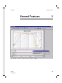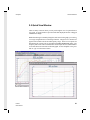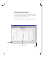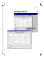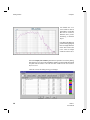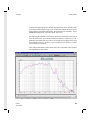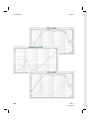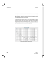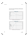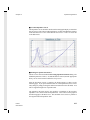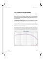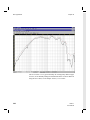
1
Contents
Loudspeaker Measurement System
User Manual
Win32 Release 4.1
LMS 4.1
User Manual
i
Contents
LMS 4.1
User Manual
© 2000 LINEARX SYSTEMS INC.
All Rights Reserved.
Tel: (503) 612-9565
Fax: (503) 612-9344
Printed in the United States of America.
July 19, 2000.
This document was produced on a Pentium-II/400 PC with WinNT-4 using Adobe PageMaker 6.5, Adobe Illustrator
8.0, Adobe PhotoShop 5.0, MathType 4.0 for mathematics typography, and SnagIt 4.3 for screen captures. Final
masters were produced using an Agfa SelectSet 9000 image setter. Help files were composed and compiled using
Windows Help Designer 2.3.
ii
LMS 4.1
User Manual
Contents
License Agreement and Limited Warranty
Carefully read all of the following terms and conditions of this agreement before opening and using the contents of this
package. The opening of this package indicates your acceptance of the terms and conditions of this license agreement. If
you are not willing to accept the terms and conditions of this agreement, then you should return the entire product, with the
package seal unbroken, to the place of purchase for a full refund of the purchase price.
■ Copyright Ownership
Both the program and the documentation are protected under applicable copyright laws. LinearX is the holder of this copyright. Your right to use the program
and the documentation are limited to the terms and conditions described herein. Use of the software unless pursuant to the terms and conditions of this
license, or as otherwise authorized by law, is an infringement of the copyright.
■ Limited Non-Exclusive License
You may: (a) use the enclosed program on a single computer, (b) physically transfer the program from one computer to another provided that the program is
used on only one computer at a time, and that you remove any copies of the program from the computer from which the program is being transferred, (c) make
copies of the program solely for backup or archival purposes. You must reproduce and include the copyright notice and label any backup copy.
You may not: (a) distribute copies of the program or the documentation to others, (b) lease, rent, grant sublicenses, or other rights to the program, (c) provide
use of the program in a computer service business, network, time-sharing multiple CPU or multiple users arrangement without the prior written consent of
LinearX, (d) translate or otherwise alter the program or related documentation without the prior written consent of LinearX.
■ Terms
Your license to use the program and the documentation will automatically terminate if you fail to comply with the terms of this agreement. Your license
terminates in the event that you receive a license for an updated version of the product that replaces this product. If a license expiration date is printed on your
documentation, or provided through other means such as a time limited electronic or software key, your license expires on the day as shown in the documentation, or on the day that the electronic or software key expires. If this license is terminated you agree to destroy all copies of the program and documentation.
■ Limited Warranty
LinearX warrants to the original licensee that the disk(s) and or electronic key(s) on which the program is recorded will be free from defects in materials and
workmanship under normal use for a period of ninety (90) days from the date of purchase as evidenced by a copy of your receipt. If failure of the product
components has resulted from accident, abuse, or misapplication of the product, then LinearX or third party licensors shall have no responsibility to replace the
disk(s) or key(s) under this limited warranty.
This limited warranty and right of replacement is in lieu of, and you hereby waive, any and all other warranties, both expressed and implied, including but not
limited to warranties of merchantability and fitness for a particular purpose. The liability of LinearX or third party licensors pursuant to this limited warranty shall
be limited to the replacement of the defective disk(s) or key(s), and in no event shall LinearX or third party licensors be liable for incidental, indirect, punitive,
or consequential damages, including but not limited to loss of use, loss of profits, loss of data or data being rendered inaccurate, or losses sustained by third
parties even if LinearX or third party licensors have been advised of the possibility of such damages. This warranty gives you specific legal rights which may
vary from state to state. Some states do not allow the limitation or exclusion of liability for consequential damages, so the above limitation may not apply to you.
In addition to the foregoing, you should recognize that all complex software systems and their documentation contain errors and omissions. LinearX, its
distributors, and dealers shall not be responsible under any circumstances for providing information on or corrections to errors and omissions discovered at any
time in the product, whether or not they are aware of the errors or omissions. LinearX does not recommend the use of this product in applications in which
errors or omissions could result in loss of life, injury, or other significant loss.
This license agreement shall be governed by the laws of the state of Oregon and shall inure to the benefit of LinearX, its successors, administrators, heirs and
assigns or third party licensors.
■ United States Federal Government Restrictions
If this software is acquired by or on behalf of the U.S. Federal government or its agencies, this provision applies. Use, duplication, or disclosure of this software
is subject to restrictions set forth in the appropriate FAR 52.227-19 and DFAR 252.227-7013 documents, as applicable. The software is "commercial computer
software" and is licensed only with "Restricted Rights". Other Federal restrictions may also apply.
LinearX Systems Inc.
9500 SW Tualatin-Sherwood Rd.
Tualatin, OR 97062-8586 USA
TEL:(503) 612-9565
FAX:(503) 612-9344
Copyright 2000, LinearX Systems Inc. All rights reserved.
LMS 4.1
User Manual
Internet: www.linearx.com
All other Trademarks are the property of their respective owners.
iii
Contents
Technical Support
LinearX provides detailed printed manuals and on-line help within the program as the primary
source for user information and assistance regarding the use of this product. If these sources do
not contain the answers to your questions, contact LinearX via any of the following methods:
Internet Email:
Internet Web:
Fax:
Tel:
[email protected]
www.linearx.com
(503) 612-9344
(503) 612-9565
Technical support is free and unlimited at this time, however we reserve the right to charge for
this service in the future as conditions, overhead, and support personnel requirements dictate.
When contacting us regarding a technical support issue, PLEASE follow these steps to aid us in
understanding and solving your problem:
(1) The About Box contains a procedure for generating a SYSCONFIG.TXT file. This file can be created by the user
through the About Box and contains all of the information about your computer system and operating system. If you
feel that your question could involve issues relating to your computer/operating system, please produce this file and
attach it along with your fax or Email question.
(2) If your question involves specific details or parameters unique to your project and problem, please include a copy of
your design files with the necessary data so that we can reproduce your problem. This is only possible if you are
communicating via an electronic means such as Email or uploading files directly to our web site.
(3) If the issue regards error messages from the program, please include an exact description of the error message
and/or address information that the program reports.
(4) If there are specific steps involved to reproduce the issue, please note these exact steps required so that we can
reproduce the problem.
Technical support hours are: Monday-Friday 9:00AM to 5:00PM Pacific Standard Time.
iv
LMS 4.1
User Manual
Contents
Contents
Chapter 1: Installation
1.1
1.2
1.3
1.4
1.5
1.6
1.7
1.8
1
System Requirements .......................................................... 3
Software Installation ............................................................ 4
Hardware Installation .......................................................... 5
Interface Cable Installation ................................................. 7
Starting the Program .............................................................. 10
Microphone MDF Setup ......................................................... 11
Analyzer Calibration ................................................................. 12
How to use the Manuals ......................................................... 14
Chapter 2: General Features
15
2.1 Tool Bars, Tool Buttons, & Control Bars ..............................
2.2 Tracking Cursor ....................................................................
2.3 Zoom, Progress Meter, and Messages ..................................
2.4 Graph Hot Spots & Popup Menus .........................................
2.5 Quick View Window ................................................................
2.6 Graph Scrolling & Panning ......................................................
2.7 Numeric Entry & Formats .......................................................
2.8 Color Select Dialog ...............................................................
2.9 Font Select Dialog ............................................................
2.10 Analyzer Block Diagram ........................................................
Chapter 3: Getting Started
3.1
3.2
3.3
3.4
3.5
LMS 4.1
User Manual
The Analyzer Control Panel ....................................................
Using QuickSet Files ..............................................................
An SPL Measurement .............................................................
An Impedance Measurement ....................................................
The Scale System ..................................................................
17
18
19
20
21
22
23
25
28
30
31
33
34
35
41
44
v
Contents
Contents
Chapter 4: File Menu
45
4.1 New ...................................................................
4.2 Open ..................................................................
4.3 Reopen ...............................................................
4.4 Save ..................................................................
4.5 SaveAs .............................................................................
4.6 Revert ...............................................................................
4.7 Load QuickSet File ............................................................
4.8 Save QuickSet File ............................................................
4.9 Print .................................................................................
4.10 Editor ................................................................................
4.11 Preferences .......................................................................
4.12 Exit .................................................................................
Chapter 5: Graph Menu
47
48
49
50
51
52
53
54
55
58
60
64
65
5.1 Parameters .................................................................. 67
5.2 Curve Library ................................................................ 69
5.3 Notes & Comments ....................................................... 75
Chapter 6: Analyzer Menu
6.1
6.2
6.3
6.4
6.5
6.6
6.7
6.8
vi
77
Parameters ........................................................... 79
Sweep Start/Stop ................................................... 89
Osc On/Off .............................................................. 90
RLC Meter .............................................................. 91
Microphone Setup ............................................. 94
PAC Interface .................................................. 95
Macro Run ............................................................. 99
Calibration ............................................................. 100
LMS 4.1
User Manual
Contents
Contents
Chapter 7: Processing Menu
103
7.1 Unary Math Operations ................................................
7.2 Binary Math Operations ................................................
7.3 Minimum Phase Transform ..........................................
7.4 Delay Phase Transform ...............................................
7.5 Group Delay Transform ...................................................
7.6 Inverse Fast Fourier Transform ......................................
7.7 Fast Fourier Transform ...................................................
7.8 Speaker Parameters ...........................................................
7.9 Tail Correction .................................................................
7.10 Data Transfer ............................................................
7.11 Data Splice ...............................................................
7.12 Data Realign ...............................................................
7.13 Curve Averaging ..............................................................
7.14 Curve Compare ..............................................................
Chapter 8: Utilities Menu
8.1
8.2
8.3
8.4
8.5
8.6
8.7
8.8
8.9
9.1
9.2
9.3
9.4
LMS 4.1
User Manual
161
Import Curve Data File ......................................................
Export Curve Data File .........................................................
Export Graphics to File .......................................................
Export Graphics to Clipboard ................................................
Curve Capture .....................................................................
Curve Editor .......................................................................
Macro Editor ...................................................................
MDF Editor .....................................................................
Polar Convertor ...................................................................
Chapter 9: Scale Menu
105
115
117
121
124
126
130
131
145
147
149
151
153
157
163
165
167
173
175
181
193
195
199
205
Parameters .........................................................................
Auto ................................................................................
Up ......................................................................................
Down ..................................................................................
207
213
215
217
vii
Contents
Contents
Chapter 10: View Menu
219
10.1 Zoom In / Zoom Out ...................................................... 221
10.2 Zoom 1X / 2X / 4X / 8X ................................................. 223
10.3 Redraw ........................................................................... 225
Chapter 11: Toolbars Menu
11.1
11.2
11.3
11.4
11.5
Show All ........................................................................
Hide All ..........................................................................
Menu Toolbars ................................................................
Status Bar .....................................................................
ToolBox .........................................................................
Chapter 12: Help Menu
12.1
12.2
12.3
12.4
12.5
viii
229
231
233
235
237
239
Contents ....................................................................
Index .................................................................
Glossary .................................................................
About Modules .......................................................
About Program .......................................................
Chapter 13: Macro Programs
13.1
13.2
13.3
13.4
13.5
13.6
13.7
13.8
13.9
227
241
243
245
247
249
251
Macro Programming .......................................................
Running Macro Programs ...............................................
Creating Macro Programs ................................................
Program Structure and Syntax Rules .............................
Debugging and Error Reporting .......................................
Planning a Macro Program ...........................................
Macro Command Reference ..........................................
Macro Command Listing ...............................................
Macro Run Dialog .......................................................
253
254
255
256
257
258
259
273
275
LMS 4.1
User Manual
Contents
Contents
Chapter 14: SPL Applications
14.1
14.2
14.3
14.4
14.5
14.6
14.7
14.8
Measuring Methods for SPL ................................................
Anechoic Chamber Measurements ....................................
Ground Plane Measurements .............................................
Half Space Pit Measurements .......................................
Near Field Measurements ...............................................
Gated SPL Measurements .............................................
SPL Response of Car Interior ....................................
Acoustical Summations ...............................................
Chapter 15: Impedance Applications
15.1
15.2
15.3
15.4
LMS 4.1
User Manual
279
280
281
282
283
288
292
297
305
Measuring Methods for Impedance ........................................
Impedance by Constant Current ...........................................
Impedance by Constant Voltage ..........................................
Using LMS for Speaker Parameters ......................................
Chapter 16: Misc Applications
16.1
16.2
16.3
16.4
16.5
16.6
16.7
277
307
308
310
315
321
Passive Network Transfer Functions ..................................
Acoustical Rub and Buzz Testing .....................................
Electrical Rub and Buzz Testing .....................................
Creating Curve Data Manually ............................................
Modifing the Mic Calibration Curve .....................................
Quality Control PASS/FAIL Testing .....................................
Measuring Inductors and Capacitors vs. Frequency ..........
323
325
327
331
337
339
343
ix
Contents
Contents
Appendix
351
Appendix A: SI Units ................................................................... 359
Index
x
357
LMS 4.1
User Manual
Chapter 1
Installation
Installation
LMS 4.1
User Manual
1
1
Installation
2
Chapter 1
LMS 4.1
User Manual
Chapter 1
Installation
1.1 System Requirements
LMS is a Win32 application and runs under the MS Windows® operating systems.
These include Win95A, Win95B(OSR2), Win98, Win NT4, and Win2000 (NT5).
It will not run under older Win3.1 systems.
LMS also uses extensive graphics. For best results a 1024 x 768 video resolution
is suggested with at least 64K (16-bit) color depth. Advanced font support for both
True Type and Adobe® Type-1 fonts is also provided. The program supports native
exported graphics in many Adobe PostScript® formats including PDF. However,
to obtain all these features requires that Adobe Type Manager (ATM) be installed
on your system.
The LMS card requires a full length ISA bus slot. If you are usinga laptop computer
which does not have slots, you will probably need to use the PAC4 portable analyzer
chassis. This enables the LMS card to be placed in the PAC4, and then communication is handled across a serial COM port between the computer and PAC4.
Recommended System Requirements:
■ Full length ISA bus slot
■ Win95, Win98, NT4 or Win2000
■ 50MB free Hard Drive space
■ 32MB RAM Memory
■ Pentium® / 500 or better
■ Video 1024 x 768 Res / 64K or 16M Colors
■ Adobe® Fonts with Adobe Type Manager®
LMS 4.1
User Manual
3
Installation
Chapter 1
1.2 Software Installation
This software requires a full Win32 operating system such as Win95, Win98,
WinNT4, or Win2000. It cannot be installed under Win32S (Win3.1).
This software requires version 4.72 or higher of the Windows common control
library COMCTL32.DLL. This will be checked during installation, and your
system will be upgraded if necessary.
Note: IMPORTANT !
If you are using NT, your NT user account must have Administrator rights.
This is necessary to install the kernel driver.
Installation Instructions:
■ Place the distribution CD into your CD-ROM drive.
■ If the CD does not AutoRun, locate and run the Setup.Exe file.
■ Follow the instructions on the screen.
■ Select an electronic or manual Registration method.
The registration will prompt you for the LMS card Serial Number, which can
be found on the LMS PCB, or the product box.
Microphone Data Format (MDF) File
During the installation, you will be asked if you have an MDF floppy disk. This
disk contains the calibration data for your M31 microphone. When prompted,
insert the floppy in Drive A: and the file will be copied to the application
directory ... LMS\MDF.
When you later start the application software for the first time, you will need
to setup/load this MDF data into the software. This will enable accurate SPL
measurements. Once loaded, the data is saved in the LMS.INI file and will be
retained and used whenever the program is started.
4
LMS 4.1
User Manual
Chapter 1
Installation
1.3 Hardware Installation
IBM-PC ISA/EISA Expansion Bus I/O Port Map 200-3FF Hex
0 1 2 3 4
200
210
220
230
240
250
260
270
280
290
2A0
2B0
2C0
2D0
2E0
2F0
300
310
320
330
340
350
360
370
380
390
3A0
3B0
3C0
3D0
3E0
3F0
5 6 7 8 9 A B C D E F
Game Controller
Reserved
LPT-3
3270 PC
Network Card
COM-4
Reserved
COM-2
Hard Drive Controller
XT/370
Floppy Drive Controller
LPT-2
BiSync Comm 2
BiSync Comm 1
Mono Video
LPT-1
EGA/VGA Video
CGA Video
Reserved
COM-3
Disk
COM-1
0 1 2 3 4
5 6 7 8 9 A B C
LMS I/O PC Port Map
LMS 4.1
User Manual
20F
21F
22F
23F
24F
LMS
25F 25F
26F
27F
28F
29F
2AF
2BF
2CF
2DF
2EF
2FF
30F
LMS
31F 31F
32F
33F
34F
LMS
35F 35F
36F
37F
38F
39F
3AF
3BF
3CF
3DF
3EF
3FF
D E F
LMS
21F
Expansion Unit
Note: The LMS analyzer card has several
parts that are static sensitive and may be
damaged by the static electricity that
may have built up in your body. The best
way to assure that no damage comes to
your analyzer is to observe precautions.
First, handle the card by the edges, avoiding contact with any of the copper traces.
Secondly, make sure to ground yourself.
This can be done by touching any metal
surface, such as the computer chassis.
Before your LMS card can be installed,
the proper I/O Port Address must be
selected. The LMS card has four possible port addresses which are selectable
by setting the jumper positions on jumper
pins P1 and P2. The base port addresses
are: 21F, 25F, 31F, and 35F.
P2 P1
21F
P2 P1
25F
P2 P1
31F
P2 P1
35F
I/O Port Selection.
5
Installation
Chapter 1
A detailed description of the LMS port locations as well as other assigned PC
port locations are given in the previous LMS/PC IO Port Map. Choose one of
the port locations and set the jumpers accordingly.
If you are not certain of the port locations of other devices operating on your
computer's bus, start with location 21F. If erratic behavior is encountered, you
may wish to try another port address.
The software driver automatically detects the presence of the LMS card, and
its I/O base address. The application software obtains this information to setup
the LMS analyzer.
Note: If you have tried all port addresses and still see erratic readings, you may
have a high memory problem, or a power supply problem. Consult your Device
Manager in the Windows Control Panel to check for memory conflicts.
I/O Port Selection.
6
LMS 4.1
User Manual
Chapter 1
Installation
1.4 Interface Cable Installation
Locate the fifteen-pin socket on the rear panel of the LMS card. Connect the LMS
interface cable assembly, shown below, to the LMS rear panel socket, using the
screws on the plug to secure the assembly to the socket. The interface cable
connects the LMS PC Card to all external audio devices by a fan out into 3 lines with
XLRs.
The black cable with the female XLR is used to connect the LMS microphone. It
is easy to remember that the black mic cable on the microphone plugs into the black
cable of the LMS card. The gray cable with the female XLR is the line input for the
analyzer.
The line input can be used for connecting external microphone preamps to the LMS
analyzer, or for directly connecting any other electronic apparatus which is being
tested. This is a balanced line level input. The remaining grey cable with the male
XLR connector is the oscillator output cable. This cable can be connected directly
to the input of an amplifier for SPL measurements, or directly to a loudspeaker when
making impedance measurements. This XLR line is unbalanced with pin 1
connected to the computer frame ground, pin 3 connected to the signal ground, and
pin 2 the active output line. The Output XLR line has an output impedance of 500
Ohms. This is to facilitate direct impedance measurements with only a 2 wire
hookup.
Microphone
Input
15 Pin Connector
Line
Input
LMS Card input
Oscillator
Output
LMS Interface Cable.
LMS 4.1
User Manual
7
Installation
Chapter 1
Note: If you will be connecting the LMS output to a power amp or other device
with unbalanced inputs, you will need to make sure that Pin 2 of the output line
is connected to the active input line of the power amp or device. Remember, Pin
3 of the LMS output is a ground line, not a signal line.
The figure below shows the LMS connectors and their functions. This schematic can be used to construct other useful cables for special purposes or to
provide easier hook-up for various tests.
A common requirement is that of loudspeaker impedance testing. For this type
of test, pins 2 and 3 of the output line need to be connected to the speaker's
terminals. Pin 1 is not used.
Osc.
Output
2
1
500
ohm
Audio Out
3
Common
Ground
Computer
Chassis
Balanced Line1
Input
2
100K
3
100K
Common
Ground
Computer
Chassis
LMS Mic
Input
2
1
3
Bal.
Input
Mic
Preamp
+8.75
VDC
LMS Interface Cable Pin Functions.
8
LMS 4.1
User Manual
Chapter 1
Installation
It is a good idea to construct a short cable consisting of a female XLR with 2 single
wires from pins 2 and 3, terminated to two alligator clips. This cable would then be
plugged into the LMS output XLR. The alligator clips can then be connected easily
to speakers for measuring impedance.
All of the input/output lines of the LMS analyzer are standard 3 Pin XLR type. You
can add your own extension cables to any of these lines as needed to suit your
requirements. The microphone has an internal hybrid preamp/line driver for
handling long cables. As much as 250Ft of mic cable can be added to the
microphone input with minimal loss at high frequencies.
The figure below can be used if custom cables are to be constructed directly to the
LMS PC Card. The pin functions are self explanatory. The return ground for the
TTL Pulse output (Pin 13) can be any of the common pins (eg. Pin 12).
Note: Be careful not to short the TTL pin to ground, or a supply voltage line. This
is a direct output from an LSTTL bus driver IC. This could damage the IC.
DB 15 Connector FemaleMIC PIN 3
1
MIC PIN 1
9
MIC PIN 2
2
COMMON
COMMON
10
COMMON
11
LINE PIN 3
4
COMMON
12
LINE PIN 2
5
TTL PULSE
13
LINE PIN 1
6
COMMON
14
OSC PIN 2
OSC PIN 3
7
15
OSC PIN 1
8
+8.75 VDC
MIC
PREAMP
3
BAL
INPUT
Note: On LMS PCBs
with serial number less
than #138203, the TTL
output is not brought
out to pin 13 on the
DB15. If you wish to
use the pulse output,
contact LinearX for
detailed information.
100K
100K
500
ohm
Osc Out
LMS Card DB15F Connector Pin Functions.
LMS 4.1
User Manual
9
Installation
Chapter 1
1.5 Starting the Program
Once the installation program has been completed, and the computer rebooted,
go to the Start Menu and locate the entry LinearX > LMS > LMS Application.
If during installation you also chose to install a group folder of icons on your
desktop, you may also start the program from that location as well.
If you have installed the program to a different folder/directory than the default,
the tutorial files will not be automatically loaded when you start the program
the first time. You will need to select File | Open from the menu and locate the
files in the actual installation folder.
10
LMS 4.1
User Manual
Chapter 1
Installation
1.6 Microphone MDF Setup
Probably the first task to be performed is to load the MDF file for your microphone.
The MDF file should have been copied during the program installation, and will be
located in the ... LMS\MDF folder.
Select the Analyzer | Microphone Setup menu item as shown below. The first tab
Mic Input shows the setup information which is initially blank. An MDF file can
be loaded into both the Mic or Line inputs, but in most cases the Line input is left
blank. We are only interested in setup here for the Mic Input.
Click the Load MDF button, and then select your MDF file in the Open MDF File
dialog. You will need to change into the MDF folder. The SN of your file will be
different. After the MDF file is selected, the data will appear in the dialog tab panel
as shown below. Click OK to save these changes permanently.
LMS 4.1
User Manual
11
Installation
Chapter 1
1.7 Analyzer Calibration
When the LMS card is first installed on a computer, it is a good idea to calibrate
the card at least once. This is due to differences in supply voltages between
different computers, which can affect the operating parameters in the LMS
system. Running the calibration routines is also a good way of checking the
system for proper operation.
Select the Analyzer | Calibration menu item as shown here. The
LMS software provides two calibration routines: INTERNAL
and EXTERNAL. Much of the LMS system is controlled via
software, rather than hardware. For this reason, there are no
adjustments required on the actual card, but are instead accomplished through the software. This process requires a minimum
of user involvement or other equipment.
Note: Before running either of the calibration routines, always
allow your computer to warm up for at least 15 minutes. While
the circuitry in the LMS card is temperature compensated, it is
necessary for the temperature offsets to be achieved before
running these routines. This will provide the best results.
Select the Internal option and then press the Run
button. The process will take about 5 minutes,
and the result should look similar to what is
shown below.
If any of the tests fail, there is probably a conflict
with another board in the system causing data
corruption.
If no LMS board is present, then the routine will
not run at all. In this case either the computer
needs to be rebooted, or there is some other
problem disabling the driver.
12
LMS 4.1
User Manual
Chapter 1
Installation
Next select the External option, and press the Run button again. The first test
requests you to measure the Line Output voltage with an AC volts meter. If you do
not have one, just keep the default value.
The system prompts you to connect the Line Output to a meter to measure the AC
voltage between pins 2 and 3. If you do not have a meter, simply leave the Output
line unconnected and hit [Enter] or click the Ok button.
Next, if you have a meter, read the voltage and enter the value. If you do not, just
hit [Enter] to keep the preset default value. The system will conduct several tests
and then ask you to connect the Output line to the Input line. Plug these two XLRs
into each other and hit [Enter].
Next, the system will ask you to connect the Output line to the Mic Input. Unplug
the Output from the previous balanced input and connect it to the Mic XLR and hit
[Enter].
The operation will end shortly after the Mic Input test. Any errors will be reported
to the dialog. If you do receive error messages, repeat the external calibration again.
You may have connected the wrong lines, or did not connect them at the right time.
Remember to follow the prompted instructions in the dialog.
LMS 4.1
User Manual
13
Installation
Chapter 1
1.8 How to use the Manuals
Nobody likes to read manuals, and it is also true that most people do not enjoy
writing them. We know that you would like to start using your new LMS system
without having to read anything, but a little knowledge can go a long way. For
this reason we recommend that the following chapters be read in total:
■ Chapter 1: Installation
■ Chapter 2: General Features
■ Chapter 3: Getting Started
These chapters will give you fundamental information about LMS, and answer
most of your fundamental questions. These chapters will tell you about how
to operate the LMS software for some of the more common types of situations
you will be encountering very early on.
There are of course many more topics covered in the remaining chapters. You
can read these as needed when you encounter more questions about specific
areas of the program.
Operating and understanding the Curve Library is of basic importance for all
purposes. You will need to know how to select curves, what the notations mean,
and how to enabled/disable curves for display.
Also, understanding the operation of the Scale Parameters dialog will be of
great importance. The LMS4 software provides a wide array of scaling options
and can display your curve data in a variety of different forms.
The three Applications chapters at the end contain a wide variety of useful
examples and information. These chapters should be reviewed so that you will
know what tips and tricks are contained within them. You may be trying to
perform similar tests or measurements that will be covered in these sections. If
you run into questions about testing, take a look in this chapter for additional
help.
All of the manual contents are also available on-line within the Help system.
14
LMS 4.1
User Manual
Chapter 2
General Features
General Features
LMS 4.1
User Manual
2
15
General Features
16
Chapter 2
LMS 4.1
User Manual
Chapter 2
General Features
2.1 Tool Bars, Tool Buttons, & Control Bars
There are 9 menus in the program, and over 60 tool buttons arranged on 7 moveable
Toolbars. Essentially the functions given on a particular menu column are provided
as tool buttons on a single corresponding toolbar. There is also a status bar shown
at the bottom of the screen which provides cursor readouts and other associated
functions. A progress meter and message display are also contained here.
There are two (2) control bars (also known as trays) shown on the main screen.
These trays autosize to hold the toolbars, and have user selectable backgrounds like
the Marble pattern shown below. One tray is fixed at the top of the screen below
the menu, and the other tray is known as the ToolBox and is a floating window.
Toolbars can be moved and rearranged simply by grabbing the handle on the left
of each toolbar. They can be docked into any of the three trays, or dragged onto the
screen by themselves as a single floating window. They can also be enabled or
disabled for display.
Toolbox
Control bar -Tray
Toolbars
LMS 4.1
User Manual
17
General Features
Chapter 2
2.2 Tracking Cursor
In the bottom status bar, the cursor system readouts are shown. The cursor will
track any data curve, based on the points in the curve. To move the cursor to
another frequency quickly, double click the left mouse button at the desired
frequency. Use the Left/Right or the Home/End keyboard arrow keys to move
along a curve. Use the Up/Down keyboard arrow keys to change to a different
curve in the same curve group. To change to a different curve group, use the
spin buttons in the status bar, or the Up/Dn arrow keys on the keyboard. The
cursor will only track curves which are selected for display.
The Absolute/Relative buttons select the cursor measurement mode. When you
press Relative another black cursor will appear at the current position. As you
move the cursor the displayed data will be calculated relative to the reference
position. Pressing the Absolute button will return to normal mode.
Cursor
Marker
Cursor Controls and Readouts
18
LMS 4.1
User Manual
Chapter 2
General Features
2.3 Zoom, Progress Meter, and Messages
There are several other segmented panels on the status bar. On the left the current
Zoom level of the graph is shown. On the right, two cells show the progress meter
and a message zone for various system messages. Data will appear in these fields
as required during program operation.
The Left/Right buttons control which vertical data is to be tracked from each curve.
A curve contains a pair of vertical data sets. Generally the Left is magnitude and
the Right is phase. However virtually any kind of mixed data can be transfered and
displayed on either side of a curve's data sets.
The preformatted graph chart is drawn on a true WYSIWYG artboard display.
Printing is performed with the exact same contents as is viewed on the screen. Both
precision Color and Black&White printing and export are supported.
Zoom Level
LMS 4.1
User Manual
Progress Meter & Messages
19
General Features
Chapter 2
2.4 Graph Hot Spots & Popup Menus
There are a number of regions defined in the graph artwork that respond to
double clicks with the left mouse button. These are hot spots that will activate
various dialogs depending on the region. For example, double clicking over
a scale region will open the Scale | Parameters dialog. The various regions
are shown below.
There is also a popup menu available using the right mouse button which
provides a listing of similar various common dialogs.
Graph Parameters
Cursor Control
Scale
Parameters
Library
Curves
Notes
Comments
Graph Parameters
20
Note Parameters
LMS 4.1
User Manual
Chapter 2
General Features
2.5 Quick View Window
There are many occasions where you may wish a tighter view of a particular area
of a graph. A special window is provided with data displayed based on a dragged
rubberband rectangle.
Rather than having to constantly change the scale factor for the graph, you can drag
a rectangle using the mouse over the range of interest. The Quick View window will
appear with a smaller scale factor and frequency range. There are two options for
determining the vertical scale as controlled in the File | Preferences dialog. The
frequency/time limits will be rounded to the nearest major division, and the number
of vert/horz divisions is the same as the main graph. To close the Quick View, press
ESC or right click the mouse button.
LMS 4.1
User Manual
21
General Features
Chapter 2
2.6 Graph Scrolling & Panning
There are two scroll bars on the graph window, one for vertical scrolling and
one for horizontal scrolling. Either or both may or may not be present
depending on the zoom level of the graph window.
You can also drag or pan the graph window directly by use of the mouse. First
press and hold the SHFT key, and then while holding the left mouse button drag
the artwork. The normal mouse pointer will be changed to a hand symbol.
Horizontal
Scroll Bar
Mouse Cursor Dragging Hand
Vertical
Scroll Bar
22
LMS 4.1
User Manual
Chapter 2
General Features
2.7 Numeric Entry & Formats
The dynamic range of numeric values can be extremely large. To handle this wide
range efficiently, LMS makes extensive use of engineering notation. These are
single character multiplier suffixes which appear at the end of a numerical floating
point (real number) value.
We are all familiar with the common usage of engineering notation for common
components such as a 10K resistor or a 1u Farad capacitor. Here, the "K" represents
1E+3 and the "u" represents 1E-6. While these are common SI suffixes that will be
familiar to most users, there are other SI suffixes that are less common. The full
list of supported SI multipliers are as follows:
SI Multipliers
Name Value Suffix Name Value Suffix
kilo
10+3
K,k
milli
10-3
m
-6
u
+6
10
M
micro
10
giga
10+9
G
nano
10-9
n
tera
+12
10
T
pico
-12
p
peta
10+15
P
femto
10-15
f
exa
+18
10
E
atto
-18
a
zeta
10+21
Z
zepto
10-21
z
yotta
+24
yocto
-24
y
mega
10
Y
10
10
10
Note that in virtually all of the
suffix chars, the following convention is used: upper case is used for
multipliers greater than unity, and
lower case is used for multipliers
smaller than unity. The only exception is the kilo suffix where
both cases are supported (K or k).
Use of the exa suffix E can lead to
confusion since the standard scientific notation uses the letter E as
well, e.g. 1.234E+5. The program
assumes that if the E character is
the last character in the number, it
is treated as the exa multiplier 10+18.
If additional numeric values follow E then it is treated as scientific.
To avoid confusion component values are never displayed with the type of units.
For example, a capacitor value of 2.4f means 2.4 femto (2.4E-15). It does not mean
2.4 Farads. It is assumed that the user already knows what the units are for the given
component (e.g. Ohms, Henrys, Farads, etc.). Please keep this in mind when you
enter component values - you do not need to add the units.
LMS 4.1
User Manual
23
General Features
Chapter 2
Entering Numerical Values
Floating point numbers can be entered in any of three forms: real number
format, scientific format, or engineering format. Examples are:
2400.75
2.40075E3 or 2.40075D3
2.40075K
(real)
(scientific)
(engineering)
A floating point number must not contain spaces. Therefore do not place
spaces between suffixes or other digits. Note that the scientific format supports
the use of either the E or D character to separate the exponent. Lower case also.
In many dialog locations throughout the program, the entry of the numeric
values is monitored and checked for range violations. For example, many
parameters will not permit either negative or zero values. If you enter such a
value in one of these locations it will be automatically corrected, typically to
a value of unity.
In some dialog locations additional constraints may be placed on the numeric
value that you enter. This is to maintain the validity of the inherent formulas
involved with the parameter.
For example, if you were entering one of the values involved with the equation
2+3=5, then some other value in the equation must be simultaneously adjusted
to maintain the validity of the equation. The program will perform many of
these tasks for you automatically.
Equation checking is performed when the focus leaves the current edit control.
This informs the program that you have finished editing a value. You can Tab
to another control or click the mouse in a different control to force the program
to check the parameter relationships.
24
LMS 4.1
User Manual
Chapter 2
General Features
2.8 Color Select Dialog
A special button control is located on many
dialogs throughout the program which provides for special editing of color selection.
Two examples of such buttons are shown here
on the right.
The center of the button displays the current color for the parameter. When you
click the button, another dialog will open to change the color.
The Color Select dialog provides many powerful and convenient features for color
selection and editing. Three different color models are supported, as well as live
mouse editing on a color wheel. Colors can be picked from presets, and new user
defined colors can be saved as well.
The dialog contains many small color pads which have the dual function of display
and selection. Clicking a color pad loads the color as the current selection. If the
current color matches one of the pads, than the pad will be highlighted.
LMS 4.1
User Manual
25
General Features
Chapter 2
Standard Colors
These are the 20 standard Windows colors. Some of the black colors are
actually masking colors, but the remainder are generally the primary VGA 16
set. If your video mode is 16 or 256 color, then choosing one of these colors
will provide for solid color. Other special colors will require dithering which
may be undesirable. Clicking on one of the pads will select the color.
Extended Colors
There are 30 additional colors provided here for quick selection. Your video
mode will need to have more than 256 colors for solid display, or they will be
dithered. Clicking on one of the color pads will select the color.
Custom Colors
There are 20 additional locations provided here for user custom colors. When
the Add Custom button is clicked, the current color will be added to the array.
The array is auto incrementing, and when a color is added it will be assigned
to the next pad. These colors will persist as long as the program is running.
Clicking on one of the color pads will select the color.
Selection
These two pads display the current and original colors. This allows you to
compare the two, or to return to the original if desired. Clicking on the Original
Color pad will make it the current color.
Add Custom Button
Clicking this button will add the current color to the Custom Colors array. The
array is auto incremented so the next color pad will be used.
Model and Parameters
There are three color model choices:
- Hue-Saturation-Value (HSV)
- Red-Green-Blue (RGB)
- Cyan-Magenta-Yellow (CMY)
The model selection controls which set of parameters appear on the sliders.
The Hue slider has a range of 0 degrees to 360 degrees. This is the Hue of color
as specified radially around the HSV wheel. All other sliders range from 0%
to 100%.
26
LMS 4.1
User Manual
Chapter 2
General Features
HSV Color Space
The large circle, or color wheel, in the center of the panel enables live color editing
by use of the mouse. While holding down the left mouse button, drag across the
wheel and the color at the point of the mouse is selected. If you go into the black
region, the last color at the edge is kept until you reenter the circle. The color wheel
represents the polar coordinates of Hue as angle and Saturation as magnitude.
The vertical slider next to the wheel controls the Value parameter. This is
essentially the overall brightness of the entire wheel. As the slider is moved, the
Value of the wheel will change between 0% black and 100% full color brightness.
LMS 4.1
User Manual
27
General Features
Chapter 2
2.9 Font Select Dialog
A special button control is located on many dialogs throughout the program which provides for special editing of font
selection. An example of such a button is shown here. When
you click the button, a dialog will open for font selection.
Choosing a font and its size is completely up to the user. It is certainly possible
to select a font and/or size that is too large for the available space in the graphics.
However, with a little experimentation you will quickly see what is possible
and what will actually work. The program positions the text items automatically either left, center, or right justified. By changing the size of a font you can
easily see how the program will position the text.
This program only utilizes vector fonts. This means that TrueType and/or
Adobe (ATM) fonts should be present. If you will be printing to a pen plotter,
you should choose a plotter stroke font such as Modern that does not require
fill, and can be easily drawn by a pen.
28
LMS 4.1
User Manual
Chapter 2
General Features
TypeFace
In this panel the number of vector font families is shown, the type of font which is
currently selected, and a list of the available fonts.
TypeSize
The size of the font in points can be selected from the list box, incremented using
the spin buttons, or entered directly in the list box.
TypeStyle
Several check boxes are provided to control the style of the font. All or none of the
options can be combined.
TypeColor
This button displays and selects the color for the font. To change the color, click
the button and the Color Select dialog will be presented.
Sample Text
A text sample of the current selection is displayed in this panel. The background
color will be automatically set depending on the color of the font. A check box
allows you to view the font in actual size, or at a different size controllable by the
spin buttons at the lower right of the panel.
LMS 4.1
User Manual
29
General Features
Chapter 2
2.10 Analyzer Block Diagram
The figure below shows the equivalent block diagram for the LMS analyzer.
The analyzer is a digitally controlled analog system, featuring log frequency
resolution from 10Hz to 100kHz. Two tracking filters are included for special
purpose measurements, or to increase SNR during SPL measurements by using
their Bandpass filter functions.
The system is also capable of performing gated measurements, to provide
semi-anechoic type data in reflective environments.
Programmable
Oscillator
Volt-Freq
Convertor
Frequency
Counter
Average
Signal
Detector
Auto-Range
Gain Set
Gated Peak
Signal
Detector
30
OSC
Gate
Output
Enable
Atten
Direct
Filter
2
Filter
1
Input
Selector
500
Ohms
Line Out
Balanced
Line Input
Mic
Preamp
LMS 4.1
User Manual
Chapter 3
Getting Started
Getting Started
LMS 4.1
User Manual
3
31
Getting Started
32
Chapter 3
LMS 4.1
User Manual
Chapter 3
Getting Started
3.1 The Analyzer Control Panel
You are now probably anxious to start using your LMS as soon as possible. If you
wish to get started immediately, this chapter will provide the necessary information
to start using the LMS in the shortest amount of time. This chapter will take you
through a fast introduction to making basic SPL and Impedance measurements.
The first item in the Analyzer Menu is Parameters. This could
also be called the analyzer control panel, since it provides direct
control over virtually all aspects of the analyzer hardware.
Another means to activate this window is by using the first tool
button in the Analyzer toolbar (shown as a seven segment
character). If you prefer to use the keyboard, the shortcut key
CTRL-A will perform the same task.
The Analyzer Parameters dialog is shown below. This is a modeless dialog,
meaning that it does not prevent other dialogs from being displayed simultaneously.
This dialog also has a RollUp/RollDown button shown in the upper right hand
corner of the title bar. Because this dialog is often left open on top of the graph, the
RollUp function reduces the size to merely the title bar, thus enabling greater
visibility of the graph underneath. There are also shortcut keys for RollUp/
RollDown using CTRL-PgUp and CTRL-PgDn. Also, the F2 key can be used to
toggle RollUp/RollDown as well.
The analyzer produces continuous
readings while this dialog is visible.
The readings are shown in the black
fields of the Meter group panel.
Most of the functions in this dialog are
clearly labeled and self explanatory.
They are covered in detail in a later
section.
To turn the OSC output On/Off, there
is a button in the lower left corner of
the dialog. This same function is also
available in the Analyzer Menu and
toolbar.
LMS 4.1
User Manual
33
Getting Started
Chapter 3
3.2 Using QuickSet Files
The Analyzer Parameters dialog provides the capability to directly change any
of the parameters individually. However, this individual control can sometimes be tedious. It is possible to save the entire contents of all the analyzer
parameters at once as a file, and then this file can be reloaded later to restore
all of the parameters together. These files are known as QuickSet files.
These files contain a snapshot of the entire analyzer parameters dialog. A
number of QuickSet files have been included with the program for some
common setups.
QuickSet files can be used to save and load your common test setups very
quickly. This eliminates the need to reset all of the individual parameters. To
save/load a QuickSet file, you must first go to the File Menu, and then choose
Load or Save QuickSet File.
There is a folder under the LMS directory tree named \Set. This is the default
folder for QuickSet files, however you can locate the files anywhere you wish.
When a QuickSet file is loaded, all analyzer parameters are set to those
recorded in the QuickSet file. The Data Curve entry is also stored/recalled with
a QuickSet file. The Data Curve is the single curve in the curve library where
the next sweep data will be placed. However, any number of curves can be
displayed on the graph simultaneously, provided they have the same type of
data. A curve library can hold 50 curves.
34
LMS 4.1
User Manual
Chapter 3
Getting Started
3.3 An SPL Measurement
In order to make a simple SPL measurement of a loudspeaker with the LMS
analyzer, you will need the following:
■ A loudspeaker to measure
■ The LMS (installation completed)
■ An audio amplifier
XLR
FEMALE
2
1
3
RCA
MALE
If your amplifier does not have XLR inputs, you will need to make an adapter
cable consisting of a female XLR and the appropriate plug on the other end for
your amplifier, like the RCA connector shown here. Since the LMS oscillator
output cable is unbalanced, you can connect the adapter cable (+) to Pin 2 and
(-), or ground, to Pin 3 of a female XLR.
Place the loudspeaker and microphone as desired. Since this is not going to be a
gated measurement, the choice of placement will determine the results. If you have
an extension cable and can locate the speaker outdoors, a ground plane measurement is the quickest to setup.
Simply place the speaker on its side on the ground, preferable on concrete or
asphalt, and place the microphone also on the ground about 1 meter on axis in front
of the speaker. If you choose to make the measurement indoors, you will also be
including the room reflections.
Plug in the LMS microphone to the
LMS microphone input cable (black
cables), and plug the oscillator output
cable into the amplifier being used.
For this example we will load the
SPL.SET file. Locate and load this
QuickSet file as shown below. After
the file is loaded, view the contents of
the Analyzer Parameters dialog.
Note: If you are not using Drive C:,
you will need to change to the drive
you installed the program on.
LMS 4.1
User Manual
35
Getting Started
Chapter 3
If the amplifier has level controls, set the level to 1/4 to 1/2 open. The LMS
oscillator can be toggled OFF and ON with the F10 key. Set the amplifier to
produce a nominal sound level from the speaker. This can be adjusted either
by the amplifier volume control, or by the LMS output level controls in the
analyzer parameters dialog.
Before starting the measurement sweep, we will create a new curve library.
Select the File | New menu item. This will clear all library curve entries, title
block data, and any notes. The library will be given the name Untitled.Lib.
Curve Library
To see what the Curve Library now looks
like, select the Graph | Curve Library
menu item. This can also be activated by
using the shortcut key F6, or the tool button
with the wavy lines. The Curve Library
dialog is shown below.
There are 50 curve entries in a given library. These entries can hold many
different types of data, possibly taken over a variety of different frequency
ranges. The Curve Library also shows which curves are selected for display on
the graph, as indicated by a check in the second G column.
A single curve is always selected as the location where the next sweep data will
be placed. This is called the data curve entry. It is indicated by the angle
brackets in the first column, and is also provided in the edit box Data Curve.
36
LMS 4.1
User Manual
Chapter 3
Getting Started
Note: Only curves of similar units can be displayed on the graph simultaneously.
The type of data units for display are defined by the first enabled curve in the list.
If you attempt to display mixed curve types, curves which do not match the first
enabled curve will be automatically disabled from display. For example, you
cannot display an Impedance curve at the same time with an SPL curve. The types
of grids and scales would not be compatible.
The Data Curve is the location of where the data of the next sweep taken will be
stored. This is a pair of angle brackets around the index number of the curve in the
grid box (table). It is also displayed in an edit field shown in the upper left hand
corner. The data curve can be selected using the edit field, or simply by double
clicking on a curve entry in the table. When a new data curve is selected, it is also
automatically enabled for display.
The remaining columns in the table show a variety of information about the curve
entries. Each curve can be given a name, and there is additional information that
can be stored with each curve as well. Other columns provide information about
the type of data in the curve, number of data points, and the line attributes for the
curve.
Most of this is self-explanatory and will not be covered here in any further detail.
For more information about the Curve Library, see the Graph Menu chapter. For
now, just exit the Curve Library dialog using the Cancel button.
We are now ready to start the sweep. Select the Analyzer | Sweep
Start/Stop menu item. Note that a shortcut key F9 can also be used
to activate this function. A tool button is provided as indicated by
the Red dot which turns Green when a sweep is active.
Sweep Button
When the sweep starts, the status bar at the bottom of the screen
will display a progress meter. A message is also displayed which
informs you how to stop the sweep using F9 or ESC. As the sweep
progresses, a blip marker is shown at the leading edge of the curve
as it is being drawn on the graph.
Scale Auto
LMS 4.1
User Manual
In a case like this where no previous data curves
exist on the graph, the scales may not be in a
position where the new sweep data is visible
while it is being drawn. It may be at the top or
bottom of the graph. However, once the sweep
is completed you can use the Scale | Auto to
bring the curve into view.
37
Getting Started
Chapter 3
You should now see a
curve similar to what is
shown above. Your SPL
data will of course be
different, since you are
measuring a different
object.
Note that in the Map area
just below the graph grid,
there is a single short line
in the same color as the
curve. Now we will put
a name on our new curve.
Select the Graph | Curve Library menu item to open the Curve Library dialog.
Note that curve #1 is now ON, and that the number of points and the horizontal
freq data items are filed in. We can now enter a name for our curve such as:
My New Curve.
Click Ok to close the dialog saving your changes.
38
LMS 4.1
User Manual
Chapter 3
Getting Started
Looking at the graph again, note that the Map legend now shows the name of the
curve next to the line sample. This is how you can easily identify the curves on the
graph with their actual names in the library. We should now save our library. Select
the File | Save menu item, and enter a name such as Test.
Note that along the status bar is a spin button. This button can be used to select which
curve the cursor tracks. You can also use the keyboard arrow Up/Dn keys as well.
When the cursor displays the curve name, you can then move along the curve using
the Left/Right arrow keys, or double click at another point on the curve, and the
cursor will jump to that point.
The Left/Right data buttons control which side of the vertical data will be tracked:
left( magnitude) or right (phase).
LMS 4.1
User Manual
39
Getting Started
Chapter 3
Let's now go back to the analyzer control panel. Select the Analyzer |
Parameters item from the menu, or use the tool button or F5.
Analyzer Parameters
As shown below, one of the group panels in this dialog is called Sweep.
This panel contains a list box titled Data Curve. This allows you to
choose the data curve for the next sweep, just as you would in the Curve
Library dialog. Providing this function here eliminates the need of
having to leave the Analyzer Parameters and open the Curve Library.
There are several other similar features offered in this panel. You can set the
Name for the data curve here as well. Also, by pressing the Graph button you
can select the data curve for display alone, and disable all other curves.
Another commonly used feature is to take static measurements from this
dialog. You can turn the Oscillator On/Off by using the lower left hand button.
This function is also provided on the main menu and on a tool button.
If you have a requirement where you wish to manually adjust the oscillator
frequency, the slider control in the Oscillator group panel provides this
capability.
The dialog also features several buttons which perform automatic unit conversion. By clicking the unit button you will be cycled through a list of units.
Note: Static measurements and readings are obtained by this dialog on a
continual basis whenever this dialog
is visible.
Note: You can change the color of the
meter readouts by clicking on the Value
or Freq black readouts.
40
LMS 4.1
User Manual
Chapter 3
Getting Started
3.4 An Impedance Measurement
Taking impedance measurements with LMS is very easy. The LMS card has a built
in 500 ohm output impedance which is connected directly to the speaker. The
software then automatically solves this voltage divider and determines the true
impedance of the load in ohms. In order to make a simple impedance loudspeaker
measurement with the LMS analyzer, you will need the following:
■ A loudspeaker to measure
■ The LMS (installation completed)
■ An adapter cable with alligator clips to connect to the speaker
XLR
FEMALE
2
1
3
TEST
CLIPS
Since impedance measurements are made by directly connecting the loudspeaker to the oscillator output XLR, you will not need an amplifier. You will
need to make an adapter cable consisting of a female XLR with a fan out to two
individual wires with alligator clips. Bring out pins 2 and 3 from the XLR to the
clips as shown in the figure here.
It does not matter which of the two wires are connected to the positive terminal of
the speaker. Polarity is irrelevant in this measurement.
Note: The direct impedance measurement method provided by LMS is only suitable
for loudspeaker impedance measurements where the load impedance is typically in
the range of 4-400 Ohms. If your load is outside this range, then a different method
such as employed by our VI-Box should be used.
There are two methods of measuring direct impedance using LMS: 2-Wire and 4Wire. In the 2-Wire mode only the Osc output is connected to the load, and the Line
Output is then selected as the Source in the Meter panel. In the 4-Wire mode, the
Line Input is also used and directly connected at the load terminals. In this way the
line cable resistance is removed from the measurement.
For this example the simple 2-Wire method will be used. There are two different
QuickSet files provided in the LMS\Set folder: ZImp2Wire and ZImp4Wire. We will
now load the ZImp2Wire.Set QuickSet file.
LMS 4.1
User Manual
41
Getting Started
Chapter 3
Select the File | Load QuickSet menu item, and
then choose the ZImp2Wire set file. Open the
Analyzer Parameters dialog, and note the changes
from the previous SPL setup.
Since we probably do not wish to overwrite the previous SPL data curve, the
first thing we should do is change the data curve selection here to #2. If you
wish you can also assign a name for the curve by clicking the name button.
If you have your speaker connected as previously described, you can now take
a static Impedance measurement simply by pressing the Osc On/Off button.
You will see the impedance value, at the static test frequency, shown in the
Value field of the Meter panel. You can move the frequency around and watch
the Impedance readout change.
We can now run a sweep by pressing F9 or using the tool button and/or menu
item selection under Analyzer. When the sweep is completed, click the Graph
button in the Sweep group panel.
You will probably need to adjust the scales for
your data, so choose the Scale | Auto menu item
as well.
Scale Auto
42
LMS 4.1
User Manual
Chapter 3
Getting Started
The graph should now show an impedance curve similar to what is shown below.
Again, your data will of course be different.
For additional information on the operation of the LMS analyzer for measurements,
and software features, read the other chapters and application information.
LMS 4.1
User Manual
43
Getting Started
Chapter 3
3.5 The Scale System
The heart of the curve graphing system is the
Scale | Parameters dialog. This dialog controls
how every type of curve is displayed, and also
defines the number of divisions on the grid as
well as the labeling on all axis.
Scale Parameters
The dialog is organized into two sections: horizontal scales and vertical scales.
Each type of data has it's own scale definition. Most of the fields and
parameters are self explanatory, but are explained in full detail in the Scale
Menu chapter.
The scaling system may seem somewhat complex when you first start working
with it. However as you work with it more you will quickly see that all of the
vertical tabs contain essentially the same information.
The powerful scaling system provides
the ability to show data curves in almost any manner desired. Both rectangular and circular plots are fully supported.
The labeling system runs fully automatic, and produces excellent labels
for most applications. If you have
some special need for custom labels,
you can disable the automatic mode
from the File | Preferences dialog.
However, in this case you will then be
responsible for manually regenerating
labels as needed whenever the scales
are changed.
44
LMS 4.1
User Manual
Chapter 4
File Menu
File Menu
LMS 4.1
User Manual
4
45
File Menu
46
Chapter 4
LMS 4.1
User Manual
Chapter 4
File Menu
4.1 New
The File | New menu item starts a new library. The
accelerator key CTRL-N can be used to activate this item
using the keyboard, or the tool button as shown above.
If your existing library has changes, and has not yet been
saved, you will be prompted to save it first.
File | New changes the name of the library to Untitled, and
initializes and/or clears some of the various system parameters, including the curve entries. You will be required to set a real name before the
program will allow you to save the library file.
LMS 4.1
User Manual
47
File Menu
Chapter 4
4.2 Open
The File | Open menu item opens an existing library.
The accelerator key CTRL-O can be used to activate
this item using the keyboard, or the tool button as
shown above.
If your existing library has changes, and has not yet
been saved, you will be prompted to save it first.
File | Open presents a dialog to choose the library file
to open. Library files have an LIB extension.
Depending on the various options in the File | Preferences dialog, different
parameters can be updated from library files, or retained as global settings
across library files.
Note:
By default the program always loads your last library when it is first started.
48
LMS 4.1
User Manual
Chapter 4
File Menu
4.3 Reopen
The File | Reopen menu item
opens an existing library, by one
of the previously stored 12 paths.
The sub menu adjacent to the
drop down menu displays the
possible choices. These paths are
updated based on your previously
opened library files.
The tool button shown above can
also be used, which will present a dialog with the same path choices as shown below.
Each path is listed on a button for selection.
If your existing library has changes, and has not yet been saved, you will be
prompted to save it first.
LMS 4.1
User Manual
49
File Menu
Chapter 4
4.4 Save
The File | Save menu item saves an existing library.
The accelerator key CTRL-S can be used to activate
this item using the keyboard, or the tool button as
shown above.
If your library has not yet been named, you will be
prompted to provide a name for the library. If it already
has a valid name that name will be kept.
When saving library files, it is generally best to create a project folder under
which all of your files for that project can be placed. This can include imported/
exported data files, graphics files, etc.
Library files have an extension of LIB. You should always use the default
extension. It is not recommended that you use other extensions, or you may not
recognize the files in the future.
50
LMS 4.1
User Manual
Chapter 4
File Menu
4.5 Save As
The File | SaveAs menu item saves the current library under
a new name. The tool button as shown above can also be
used to activate this item. A dialog will be presented to
specify the file name and/or folder.
When saving library files, it is generally best to create a
project folder under which all of your files for that project
can be placed. This can include imported/exported data
files, graphics files, etc.
Library files have an extension of LIB. You should always use the default
extension. It is not recommended that you use other extensions, or you may not
recognize the files in the future.
LMS 4.1
User Manual
51
File Menu
Chapter 4
4.6 Revert
The File | Revert menu item allows you to abort the
current library file changes, and reload the last saved
version of the library. The tool button as shown above
can also be used to activate this item.
A dialog will be presented to ask you to confirm this
action. All changes to the library will be lost when the
previously saved version is reloaded.
52
LMS 4.1
User Manual
Chapter 4
File Menu
4.7 Load QuickSet File
The File | Load QuickSet File menu item opens a QuickSet
file, and loads the configuration data into the Analyzer |
Parameters dialog. The tool button as shown above can also
be used to activate this item as well as shortcut CTRL-L.
QuickSet files store configuration parameters from the
Analyzer | Parameters dialog
File | Load QuickSet File presents a dialog to choose the QuickSet file to load.
QuickSet files have an SET extension.
LMS 4.1
User Manual
53
File Menu
Chapter 4
4.8 Save QuickSet File
The File | Save QuickSet File menu item saves a
QuickSet file. The tool button as shown above can also
be used to activate this item.
QuickSet files store configuration parameters from the
Analyzer | Parameters dialog.
File | Save QuickSet File presents a dialog to specify the QuickSet file name
and folder to save. You may choose to save QuickSet files on a project basis,
or place the files in the common Set folder.
QuickSet files have an extension of SET. You should always use the default
extension. It is not recommended that you use other extensions, or you may not
recognize the files in the future.
54
LMS 4.1
User Manual
Chapter 4
File Menu
4.9 Print
The File | Print menu item is used to print the main graph
window data. The accelerator key CTRL-P can be used to
activate this item using the keyboard, or the tool button as
shown above.
The Print item opens a dialog for printing control. From
here the artwork generated in the program can be printed to
any output device currently supported in your Windows
system.
The graph used in the program has a layout of 10 inches wide by 8 inches high.
Printing at a scale factor of 100% will require landscape orientation on 8½ x 11 letter
size paper. This is the default mode for the printer setup. For portrait printing, use
a reduced scale factor such as 80% or less.
Printer Configuration
This panel displays the configuration for the currently selected printer. When you
start a print, this configuration will be used. To change the configuration use the
Setup button at the bottom of the dialog box.
LMS 4.1
User Manual
55
File Menu
Chapter 4
Color Options
This panel provides two options which control how the graphics are printed.
If the Color/Gray option is selected, and you are printing to a black & white
device, the colors in the artwork will be dithered to produce gray levels.
When the Black & White selection is used, all colors in the artwork graphics
will be printed as black regardless of the printer. This is a very useful feature
when printing to a dot matrix device. Gray halftones of low resolution on small
lines or fonts may often result in unreadable graphics. Printing all colors as
black will eliminate this problem and produce better looking plots on low
resolution devices.
For printing on laser or ink jet printers where higher resolution is available, it
may be a matter of choice as to the representation of color. Gray lines of
varying density may help to produce more identity between multiple lines on
the graphs. With the low cost availability of color ink jet printers today,
printing in color will usually be the most popular choice.
Location Options
This panel provides two options which control where the graphics are printed
on the page. If you are printing in full size, neither option will be much different
since the artwork will mostly fill the page regardless. However, if the graph is
printed at reduce size, the image will appear either in the middle of the page or
in the top left corner.
The Center of Page positions the artwork in the center of the available printing
area. The printing area is dependent on the page size selected for the printer.
The Corner of Page option positions the artwork at a corner of the available
printing area. The printing area is dependent on the page size selected for the
printer, and the specific corner will very depending on whether landscape or
portrait orientation is in use.
56
LMS 4.1
User Manual
Chapter 4
File Menu
Scaling Options
This editing field allows you to specify the amount of enlargement or reduction in
the magnification of the printed image. The value is entered in percent. A full size
100% plot represents an artwork width of 10 inches and a height of 8 inches for the
standard sized graphs.
Setup Button
Use this button when you wish to change the selected printer, and/or configuration.
When this button is pressed another dialog will open to change the printer/port
selection. These dialogs are produced from the printer driver. The contents of these
dialogs will be different for various printers. An example is shown below.
LMS 4.1
User Manual
57
File Menu
Chapter 4
4.10 Editor
The File | Editor menu item allows you to open and
view/edit a file with your currently selected text editor.
The tool button as shown above can also be used to
activate this item.
The default editor is set to NOTEPAD.EXE. However
you can easily change this to your favorite text editor
through the File | Preferences dialog.
There are many occasions in the program where you may wish to view or edit
the contents of a text file. This arises frequently when you are importing/
exporting text data. All text files exported by the program have the default
extension TXT.
File | Editor presents a dialog to choose the file to open with the editor.
58
LMS 4.1
User Manual
Chapter 4
File Menu
The image above shows a text file opened with the NOTEPAD editor.
LMS 4.1
User Manual
59
File Menu
Chapter 4
4.11 Preferences
The File | Preferences menu item opens a dialog that
contains additional parameter settings for the program.
These are parameters which are changed on a less
frequent basis, or provide optional behavior.
Preference parameters are stored in the LMS. INI file as
global characteristics, and are not loaded or stored in
library files.
Editor Path
This is the path to the editor you wish to use when opening text files for viewing
or editing inside the program. The default choice is the Window's
NOTEPAD.EXE basic editing program. You can choose your own favorite
editor by using the Browse button, and selecting your editor's EXE file.
60
LMS 4.1
User Manual
Chapter 4
File Menu
General
There are several check boxes which enable/disable general options in the program.
The Show Splash Screen controls whether the initial introduction screen appears
when you start the program. The Auto Backup Library Files will automatically
create a BAK version of your library file each time you save it. The Quick View
Scale from Data controls how the vertical auto scale is generated for the QuickView
graph. When disabled, the vertical scale is produced by the major division values
of the original graph. When enabled, the scale is adjusted to fit the data within the
bounds of the selection rectangle. The Auto RollUp Analyzer Parameters will
automatically roll-up the analyzer parameters dialog when a sweep is started, and
roll it down when the sweep is completed.
Curves
The Automatic Curve Notes enables transfer of the curve info fields from the first
two displayed curves into the Note & Comment graph fields. This is a handy feature
which automatically transfers and displays the extra curve info on the graph page.
However, if you wish to create your own graph notes, you will need to turn this off.
The Beep At End of Sweep function produces an audible beep when a sweep is
completed. The New Library Auto Color will create a rotating group of five
different colors whenever a File | New library is performed.
Scales
The Automatic Labels option controls whether or not the system generates it's own
labels for all scales automatically. If this is enabled, the labeling features in the
Scale | Parameters dialog are grayed out. You can disable this if you wish to create
special labels yourself. The Auto Up/Dn Right Vert Data option selects whether the
right side vertical data in the curves is controlled by the scale adjustment functions.
It is common that you may not want the phase (right vertical data) to change with
scale functions. However, if you have other data than Phase in your curves, you
may need to enable this features
Cursor Style
The bitmap used for the tracking cursor can be selected here. There are several
possible choices. The blinking rate of the cursor can also be controlled by entering
a numeric value in the edit box.
LMS 4.1
User Manual
61
File Menu
Chapter 4
Relative Cursor Mode Horz Data
When taking relative cursor measurements, this option provides two different
readout modes for the horizontal data. You can have the horizontal value
represent the absolute true value at the cursor, or the horizontal difference
between the reference point and the current position of the cursor. This would
be similar to what happens with the vertical data.
Optional Library File Data
These options determine whether some configuration parameters will be
treated as global or library specific. For example, when opening a library file
one may wish for the current graph fonts and color settings to remain
unchanged. Likewise, one may wish that the toolbar locations remain the
same, and not be affected when a library is opened. Conversely, if you want
to restore all of the full configuration elements by each library file when it is
opened, you can enable these options.
Control Bar Texture
These are selectable backgrounds which can be
used in the control bars located at the top and in
the Tool Box.
The color depth of these texture patterns vary
from 4-Bit to 24-Bit. Depending on the mode of
your video system, some may not be suitable for
display.
You can create your own bitmaps as well and
place them into the ControlBarTexture folder.
The program will automatically load them for
selection the next time it is started.
There is also a palette file LMS.PAL which should
be used if you are creating 256 color bitmaps. All
files must be BMP format.
62
LMS 4.1
User Manual
Chapter 4
File Menu
Analyzer Configuration
The fields in this panel represent some of the calibration and/or operational control
data for the analyzer. There are also a couple of additional check boxes which
enable/disable certain specific system functions. Most of these parameters should
not be changed by the user.
The two exceptions are the TTL pulse width, and RT60 threshold delta. These
values can be adjusted as needed by the user.
LMS 4.1
User Manual
63
File Menu
Chapter 4
4.12 Exit
The File | Exit menu item is used to terminate the
program. The accelerator key CTRL-Q can be used to
activate this item using the keyboard as well.
When this option is selected the system checks to see if
any changes have been made since the library was last
saved. If changes have been made, then a dialog box
will appear with three options for exiting the program.
If the current library name is Untitled you will always
receive this message.
Use the YES button if you wish to save the library, and another dialog box will
appear to allow you to enter a new file name if the current name is Untitled. If
the current name is valid, the file will be updated. The program will exit after
saving the file.
Use the NO button if you do not wish to save the current library as a file, or do
not wish to update the existing file on disk. The program will exit after pressing
this button.
Use the CANCEL button if you wish to abort the exiting process. You will be
returned to the program after this button is pressed.
Note:
When you exit the program, all of the configuration data is stored in the
LMS.INI file and will be restored the next time you start the program.
64
LMS 4.1
User Manual
Chapter 5
Graph Menu
Graph Menu
LMS 4.1
User Manual
5
65
Graph Menu
66
Chapter 5
LMS 4.1
User Manual
Chapter 5
Graph Menu
5.1 Parameters
The Graph | Parameters menu item will
open a dialog which controls the appearance
of graph artwork within the program. The
tool button as shown above can also be used
to activate this item.
This dialog allows you to define the colors, lines, and fonts commonly used on the
graphs of the program. By using these parameters a very wide range of different
graph designs can be easily produced. Graphics dimensions are always given in
mils (1/1000 of an Inch). For example a 10 mil line is 0.010 Inches.
Frame Parameters
The Background color is applied across the entire area of the graph page. The Note
Underline controls the color and width of the lines under the user note text. The
Large Frame Line controls the color and line width of the border around the graph.
The Small Frame Line controls the color and line width of the sub divider border
lines between different sections of the title block, note block, and map block.
Grid Parameters
The Background color is applied inside the region of the grid itself. The Border Line
controls the color and width of the border surrounding the grid. The Major Div
controls the color, width, and line style of the major division lines drawn on the grid.
The Minor Div controls the color, width, and line style of the minor division lines
drawn on the grid.
Font Parameters
There are six tabs in this panel that control the
fonts used in different regions of the graph
artwork. The titles are self explanatory. The
color can be changed directly by clicking the
Color button, and the font can be changed by
clicking the Font button.
Note: Win9X has no support for line styles
other than Solid when using line widths larger
than 1. WinNT4 does support this, however
non-Solid line drawing is extremely slow. PostScript printing/export is always supported.
LMS 4.1
User Manual
67
Graph Menu
68
Chapter 5
LMS 4.1
User Manual
Chapter 5
Graph Menu
5.2 Curve Library
The Graph | Curve Library menu item will open a dialog which controls the
library of curves used in the program. The tool button as shown above can also be
used to activate this item, as well as the shortcut key F6. This is a dialog which is
frequently used.
Library Curves are arbitrary data that can represent measurements obtained by the
analyzer, generated by processing functions, or externally imported into the
program. There is a maximum of 50 library curves.
Library curves can contain a wide variety of different types of data, measured
across different frequency ranges and vertical axis. Therefore, any curve can
contain data which is not necessarily in the same frequency range as that currently
in use by the scale system of the program. However, there is a means to realign this
data to the current scale frequency range or any other if desired.
Since the frequency data points contained in each curve may be different, the data
grid displays the number of data points, frequency range, and type of data for each
of the curves.
The names used for curves can be set and/or changed by the user. When data is
initially placed into the curves through various operations, a default name will
usually be created by the program. For example, when you import a curve from a
file, the file name will be inserted as the curve name. You can change the name later
to whatever you prefer.
The program also performs a wide array of housekeeping chores, by filling in
various types of comments into the Info curve fields automatically. For example
when sweep measurements are taken, a date/time stamp note is placed in the Info
fields denoting when the measurement was taken.
LMS 4.1
User Manual
69
Graph Menu
Chapter 5
Parameters
A large data grid (table) displays the 50 library curve entries. The points
column informs you whether each entry actually contains data or is empty. The
names of each entry are editable by the user, and in many cases will be initially
created by processing or import operations. Each curve can be individually
enabled for display on the graph, and has definable line color, width, and style.
A library curve is actually a pair of curves, with a left side vertical data type,
and a right side vertical data type. In most cases these represent magnitude and
phase respectively, although any data can be transferred to either vertical side.
The Data Curve edit box allows you to select which of the curves will be used
for the next sweep measurement data. This can also be chosen by double
clicking on any curve entry. You can also use the shortcut key CTRL-D.
Single or multiple curves can be selected by holding down the Shift or Ctrl keys,
while selecting another curve with the mouse. All of the curves can be selected
at once by using CTRL-A.
The Show All and Hide All buttons will enable or disable all of the curves for
display on the graph. It is often useful to use the Hide All button to shut off all
curves. You can also toggle selected curves for display by using CTRL-G.
70
LMS 4.1
User Manual
Chapter 5
Graph Menu
The Cut button will first copy the selected curves to the Windows's Clipboard, and
then delete them from the library.
The Copy button will copy the selected curves to the Window's Clipboard.
The Paste button will paste the copied curves from the Window's Clipboard starting
at the currently selected curve entry. If the block of copied curves extends past the
last entry, they will be wrapped around to the top of the library. This provides the
means to move or copy curves from one location to another. Since the clipboard
is used, a different library can be loaded and the curves pasted into that library.
The Paste button will only be enabled if one or more curves are present in the
clipboard. When a curve is present, the Paste button will show hint text containing
the name and parameters of the curve. For multiple curves, a list of the original
curve entry numbers will be displayed.
The Delete button will delete the selected curves from the library. Deleting all of
the curves at once can be performed by pressing CTRL-A and then using Delete.
Check Boxes
The check box Same Line Type will force the same line attribute settings for all
curves. This means color, width, and line style. Right Lighter will make the right
side vertical data curve (such as phase) a lighter color shade then the left vertical data
curve. This is sometimes useful for distinguishing between the left/right data shown
on the graph.
The Left (Magnitude) and Right (Phase) check boxes enable/disable the display of
either vertical type data on the graph.
Table/Grid Columns
The Curve column shows the number of the entry from 1 to 50. When an entry is
selected as the data curve, a pair of angle brackets are shown around this number.
The data curve entry can be selected by double clicking on an entry or by using the
Data Curve edit box.
The G column provides an array of check boxes which are used to select the curve
entry for display on the graph. The Name column can be edited to enter a name for
each curve entry.
LMS 4.1
User Manual
71
Graph Menu
Chapter 5
The Info column provides access to some additional notes which can be
attached to each curve. If there are additional notes, the field will say Yes. Click
on the ellipse button to open the info editing dialog.
The Horz Data Range column provides an abbreviated message giving the
range of horizontal data. If it is a frequency axis, it will show the lowest and
highest frequency values in the curve.
You can click on the ellipse button, and another
dialog will open which allows you to realign the
data to a different frequency range, log or linear
axis, and number of data points. For more details
on this function, see the Processing | Data Realign chapter and section.
The Left Vert and Right Vert columns provides the ability to change the type
of vertical data represented in the curve. For example you may wish to change
a voltage measurement which actually represented current through a shunt to
Amps. The type of units defined here determine which scale set will be used
when drawing the curve on the graph.
The Points column displays the number of data points in the curve. The
maximum number of data points in a curve entry is 4096.
The Style, Width, and Color columns determine the line attributes used to draw
each curve. The width parameter is given in mils (1/1000 of an Inch). If the
Same Line Type check box is enabled, all curves will have the same style, width,
and color. If the Right Lighter check box is enabled, the right side curve
(generally phase) will be drawn with a lighter shade of the specified color.
Note: Win9X does not support drawing complex lines larger than 1 pixel width.
This means dash, dot, etc. WinNT is required to support these styles.
72
LMS 4.1
User Manual
Chapter 5
Graph Menu
Curve Info Dialog
When an ellipse button in the Info column is clicked, the Curve Info dialog will
appear as shown below. This dialog allows you to enter/edit additional notes for
each curve entry.
The Transfer options panel provides some handy features for displaying the curve
info text on the graph page. If the Auto Copy is enabled, then the first two enabled
curves will have their notes automatically transferred to the graph note area. This
is a dynamic process which occurs automatically as different curves are selected for
display. Since there are only 8 text lines in the graph notes, and 4 lines in a curve
entry info, only the notes from the first two displayed curves can be shown in the
graph notes area.
The other two options, Copy Info Text to Left/Right Notes, provide a manual
method to transfer the content of the curve info to the graph notes when desired.
LMS 4.1
User Manual
73
Graph Menu
74
Chapter 5
LMS 4.1
User Manual
Chapter 5
Graph Menu
5.3 Notes & Comments
The Graph | Notes & Comments menu item will open a dialog which allows you
to enter user defined notes and identification information. The tool button as shown
above can also be used to activate this item.
Automatic Curve Info Notes
If this feature is enabled, the graph note fields are filled automatically from the curve
entry info fields. Manual editing of the notes is disabled.
Left Page / Right Page
There are eight lines of possible notes which can be entered, four on each of these
two tabs. The note lines will appear on all of the graphs. The amount of text which
can be entered depends on the size of font currently selected.
Title Block Data
There are three fields provided to enter a company name, personal name, and
project name. The fields could also be used for other types of record keeping data.
The fields will appear in the title block of all graphs.
LMS 4.1
User Manual
75
Graph Menu
76
Chapter 5
LMS 4.1
User Manual
Chapter 6
Analyzer Menu
Analyzer Menu
LMS 4.1
User Manual
6
77
Analyzer Menu
78
Chapter 6
LMS 4.1
User Manual
Chapter 6
Analyzer Menu
6.1 Parameters
The Analyzer | Parameters menu item will open a modeless
dialog which controls all of the interaction with the LMS
analyzer hardware. The tool button as shown above can also
be used to activate this item, or the shortcut key F5. Selecting
the menu item, tool button, or shortcut key again will toggle
this dialog to close.
This dialog is modeless, meaning that it does not lock out other operations in the
program. You may leave this dialog open and continue to open other dialogs or
activate other program functions.
This dialog also supports the Roll-Up/Roll-Down feature. When leaving this dialog
on the screen, it is helpful to reduce its size so that the graph underneath is visible.
The first double arrow button in the top right corner of the title bar controls this
feature. However, you can also control the roll function by using the CTRL-PgUp
and CTRL-PgDn or the toggle key F2.
There is also an option in the File | Preferences dialog which controls the automatic
roll-up during a sweep. This allows full view of the graph during a sweep.
LMS 4.1
User Manual
79
Analyzer Menu
Chapter 6
Oscillator Panel
The Output Level edit box is used to set the output level from the sine wave
oscillator. This edit box also contains a spin button, which can be used to adjust
the level up or down by about 3%. The maximum output level is around 5Vrms.
A units button directly follows the edit box, and can be used to toggle through
different units for the output level including Volts, dBV, and dBm.
The Frequency edit box operates in much the same way. The low frequency
limit is 10Hz and the upper frequency limit is 100kHz. This frequency is the
static frequency when the system is not performing a sweep. The spin buttons
will change the frequency by about 1% increments. A units button is also
provided. The frequency can be swept manually by use of the slider control.
The range of the slider is 10Hz-100kHz.
Mode Panel
There are two measurement modes provided: Precision and HiSpeed. In the
precision mode a settling algorithm is employed to produce the most accurate
and stable data. In high speed mode, only a single measurement is taken at each
frequency to provide maximum sweep speed.
Gating Panel
Gating is a technique where the oscillator and meter are both turned off/on in
a synchronous repetitive pulsed fashion. This is often used during SPL
measurements to remove the reflections of boundaries in the measurements.
Further information on gating is covered in the following pages.
Meter Filters 1 & 2
The controls used for setting the two meter filters are identical. These filters
appear in series to the Meter and, therefore, control the characteristics of the
measurement. Each filter has four controls which can be adjusted: the Filter
Type, the Osc Freq Tracking Enable, the tracking frequency Ratio when
tracking is on, and the filter's fixed Frequency when not in the tracking mode.
These filters can be used whether or not gating is active. The filters are simply
used to control the frequencies where the meter will respond. Using these filters
allows various types of different measurements to be made, or improve the
quality of the testing by reducing noise bandwidths.
80
LMS 4.1
User Manual
Chapter 6
Analyzer Menu
Filter Type
There are four filter types which can be independently set for each filter. Each filter
can be designated as either a Bandpass, Bandreject, Lowpass, Highpass or -Flatfilter. Characteristics for each filter type are as follows.
5
dBm
< Magnitude >
d B m Vo l t a g e M e a s u r e m e n t
< Phase >
Deg
0
180
135
Filter Shapes:
Bandpass & Bandreject
- 5
90
-10
45
-15
0
-20
-45
-25
-90
-30
-135
C
-35
20
Fr e que nc y
100
500
1k
Hz
5k
10k
Bandpass Filter
The Bandpass filters have a Q of 1 with a first order (6
dB/Oct) slope at both sides of the center frequency as
shown below. When both Meter Filters are set up as
bandpass filters, their combined slope is 12 dB/Octave,
as illustrated below. Both filters are typically set as 1:1
tracking bandpass filters when making SPL measurements, which ensures maximum noise rejection. This
greatly reduces the effective noise floor by as much as
30-40 dB.
-180
20k
Bandreject Filter
The bandreject filters have a sharp attenuating characteristic shown by a single
bandreject filter. These filters have a depth of typically 40dB attenuation at the
center. When used in sweeps, misalignment between the Osc frequency and the
Filter notch frequency will limit this attenuation depth to between 30-40dB. By
combining both filters as bandreject, a notch with a depth of 60-80dB can be
produced for quasi-distortion measurements.
5
dBm
< Magnitude >
d B m Vo l t a g e M e a s u r e m e n t
< Phase >
Deg
0
180
135
Filter Shapes:
Lowpass & Highpass
- 5
90
-10
45
-15
0
-20
-45
-25
-90
-30
-35
Lowpass Filter
The Lowpass filter has a rolloff rate of 12 dB/octave
(2nd order) as shown in the graph Notice the rolloff
knee has a flat characteristic up to the corner frequency of the filter. Setting both Meter Filters as
Lowpass filters results in 24 dB/Octave (4th order)
attenuation. Lowpass filters are typically used to
limit the upper frequency range of the system.
-135
C
20
Fr e que nc y
100
500
1k
Hz
5k
10k
20k
-180
Highpass Filter
The Highpass filter also has a rolloff rate of 12 dB/Octave (2nd order). Setting both
Meter Filters as Highpass filters results in a 24 dB/Octave (4th order) slope rate.
Highpass filters are typically used to restrict the low frequency range of the system.
LMS 4.1
User Manual
81
Analyzer Menu
Chapter 6
Tracking
Meter Filters have two frequency modes. The filter can be either set at some
discrete fixed frequency or set to track the oscillator's changing frequency
during a sweep. When a filter is set to track mode, the frequency of the filter
is swept from high to low frequencies at a Ratio of the osc frequency.
When tracking is turned on, the Ratio parameter is active. When tracking is
turned off, the discrete single Frequency parameter is active.
Gate Timing Panel
The four parameters on this panel all relate to setting the Gate operation when
a gated measurement type is in use, such as when making quasi-anechoic SPL
measurements in the SPL Gated data type. These are:
- Osc Off duration time (Toff)
- Osc On duration time (Tosc)
- Meter Delay time (Tdly)
- Meter On duration time (Tmtr)
Setting these four controls is a straightforward and simple process. Each
control has a specific set of requirements and/or rules that will be given shortly.
Oscillator On Time
Oscillator
Meter On Time
Meter Delay
Time
Meter
Gate
The oscillator is first programmed to produce a burst of sinewaves
for a period (Tosc). The meter input is initially turned off, but after
a preset amount of delay time (Tdly) expires is turned on. The meter
input stays open for another period of time (Tmtr) while it captures
the incoming signal and measures its level. The meter will only see
or respond to the input during time (Tmtr).
When a burst of sinewaves pass through a transfer function of unknown
characteristics (such as a loudspeaker), the leading and trailing edges of the
resulting output amplitude envelope must be expected to contain transient
distortion. This is why the meter does not open at the beginning of the oscillator
on time. It ignores the leading edge transients. Also, the meter must close
before the oscillator turns off in order to ignore the trailing edge transients.
Calculating the times required starts with understanding where the nearest
reflecting boundaries are in relation to the loudspeaker source and the measurement microphone.
82
LMS 4.1
User Manual
Chapter 6
Analyzer Menu
Note: The lowest frequency that can be measured will be determined by the largest
meter on time that can be tolerated, before reflections are included.
Total Time=10 Ft./8.8mS
DUT
5 Ft.=4.4mS (.0044S)
5 Ft.=4.4mS (.0044S)
Closest Reflection
Boundary
The layout shown here depicts a typical situation. Here
a single reflecting boundary is shown as the limiting
factor. In order to find out what the maximum meter On
time is that can be used, it will be assumed that 25% of
the meter on time will be used as a dead time safety
margin for hold off delay.
The following time equations are now given for the
maximum time window: (Treflection=Total boundary
reflection path time)
Tmtr dly
Tmtr on
Tosc on
Tosc off
=
=
=
=
(Treflection+4xTmic)/5
Treflection-Tdly
Tmtr on x 2
20mS (default)
For the figure above, the total reflection path time is about 9mS. The meter delay
time would be (9+2.8x4)/5=4mS, assuming a mic distance of 1 meter or about 2.8
mS. The meter on time would be 9-4=5mS, and the osc on time would be 10mS.
The units for the time parameters can be changed by the user. There are also
equivalent distance units provided as well, based on the velocity of sound in air.
The setting of the time parameters can also be done
much more simply by using the Gate Time Calculator
button. This will open another dialog which allows you
to setup all the timing parameters by entering the source
and reflection path distances.
It is important to understand the effect that gating has on
the low frequency response of a measurement. The
shorter the Meter On time, the higher the low end cutoff
frequency. The low frequency cutoff can be calculated
by inverting the Meter On time (1/Tmtr). In order for wide bandwidth measurements to be made to very low frequencies, it is obvious that the limiting factor is
the measurement environment.
LMS 4.1
User Manual
83
Analyzer Menu
Chapter 6
Note: If full range measurements are to be made down to low frequencies such
as 20Hz; ground plane, anechoic, half-space measurements, or near-field
techniques are required. These are discussed in the SPL Applications chapter.
Meter Panel
The two list boxes select the type of data and the source for the measurement.
The Source list box contains the following selections:
Osc Internal
Line Output
Line Input
Mic Input
Note: The OSC INTERNAL selection monitors the direct oscillator level, it is
not effected by the condition of the OSC On/Off setting. This source is always
ON. It does follow the OSC Level.
By selecting the Line Input, external levels can be measured from other
sources. For example, this input line could be connected to the output of a
power amp to measure the output level from the amp. (+20dBm maximum).
Selecting the Mic Input will measure the level at the LMS microphone input.
Note: If the SPL data type is selected, along with the Line Input or Mic Input,
the MDF setup data will be used to produce the actual SPL measurements.
The Data list box contains eight different selections as described here:
Volts
The oscillator produces a continuous or gated sinewave tone for each frequency point and the meter measures the level at the selected source. The
oscillator then steps to the next frequency and the process is repeated.
SPL
Same as Volts, but with the additional computation of SPL as defined by the
assigned MDF data for either the Mic or Line inputs.
Impedance
The impedance data type is specifically intended for measuring the impedance
of a loudspeaker or many other passive electrical devices. The measurement
is based on the 500 Ohm output impedance of the line output and the resulting
voltage divider formed with the load. Either the Line Output or Line Input can
be selected, for 2-Wire or 4-Wire impedance measurements respectively.
84
LMS 4.1
User Manual
Chapter 6
Analyzer Menu
Since the oscillator output is being taken via the analyzer's internal 500Ω load
resistor, the impedance measurement is the voltage divider type. The LMS system
will automatically remove the effect of the internal 500Ω source and record the level
in actual Ohms.
Inductance, Capacitance
These data types produce measurements which contain either Henrys or Farads.
The setup for these data types would be the same as that of impedance.
The computations assume that the impedance being measured is a pure reactance.
This is different from an RLC bridge, which separates the resistive component.
Measuring reactive components with LMS is somewhat more complex than using
an RLC bridge or meter, and the user should study the pertinent information
provided in the Miscellaneous Applications chapter.
Polar Volts
The polar data type is used to perform a true polar sweep. The oscillator frequency
is held constant, and the TTL output is pulsed for each data point. This would
normally be used to control a stepper motor turntable. The frequency is that set by
the OSCILLATOR section's FREQUENCY parameter. The number of data points
selected should equal 360 degrees divided by the degrees per pulse of the turntable.
Polar SPL
Same as Polar Volts, but with the additional computation of SPL as defined by the
assigned MDF data for either the Mic or Line inputs.
RT60
The RT60 data type is used to produce a decay curve showing the time required for
a given level to decay 60dB at a given frequency. This is commonly used for
measuring the characteristics of a room or auditorium. This sweep turns on the OSC
for five seconds to saturate the room with sound and allow the standing waves to
build, and then turns it off and takes a series of measurements as the level falls. Due
to noise in the environment, analyzers rarely measure the actual time for the level
to drop a full 60dB. Rather, they measure the time required for the level to drop a
finite amount, and then extrapolate to determine the time required to reach 60dB.
With LMS, the dB differential can be selected by the user in the File | Parameters
dialog. Depending on the level of noise in your environment, you may need to
adjust this lower, or may be able to set this higher as desired.
LMS 4.1
User Manual
85
Analyzer Menu
Chapter 6
Typically 10-30 data points are taken for reverb time measurements. This
measurement does require a total of about 10 seconds per frequency data point.
It should also be noted that due to the random decay characteristics and
standing waves in many rooms, every RT60 sweep will have slightly different
curve results. Decay characteristics tend to be very nonlinear.
The two black fields display the active measurements for the Value and Freq
of the analyzer source. You can change the color of the readouts by clicking
on the fields. You will be toggled through a list of preset colors.
The type of value units will depend on the type of data. Unit buttons are
provided for both readout fields to change the form of the displayed data.
Note: Static measurements are performed automatically and continuously
whenever this dialog is visible.
Sweep Panel
The controls in this panel determine where the sweep data will be placed in the
curve library, over what frequency range, and with what resolution. The Lo/
Hi Freq edit boxes determine the limits of the sweep. The Points edit box
defines the number of log spaced points to be measured between these two
frequency limits. The Up/Down option determines whether the sweep progresses
up or down in frequency.
The Data Curve list box provides selection of the library curve where the next
sweep data will be placed. This special list box shows the type of data contained
in each curve. After a sweep is completed, this will be updated. Any curve
which is currently being displayed on the graph is denoted by Red vertical lines
between the zones of each curve entry.
To enter or edit the name of a curve, press the Name button. An edit box will
appear for entering the curve name. When your editing is done, click Name
again to save your changes or Cancel to abort them.
In many cases you may wish to display various curves on the graph. Clicking
the Graph button will show the selected curve on the graph by itself.
When you are ready to start a sweep; use F9, the sweep tool button, or the Sweep
item on the Analyzer menu.
86
LMS 4.1
User Manual
Chapter 6
Analyzer Menu
Control Panel
Three buttons are shown on the control panel. The first button Osc On/Off will
toggle the oscillator On/Off. This can also be done from the Analyzer menu/toolbar,
or by using the shortcut key F10. This only pertains to static measurements, since
the oscillator is automatically turned on during a sweep.
The TTL Pulse button will produce a single pulse at the TTL output.
The Gate Time Calculator button will open another dialog for setting up the gate
timing values. This was previously described.
LMS 4.1
User Manual
87
Analyzer Menu
88
Chapter 6
LMS 4.1
User Manual
Chapter 6
Analyzer Menu
6.2 Sweep Start/Stop
The Analyzer | Sweep Start/Stop menu item will begin or end a sweep measurement. The tool button as shown above can also be used to activate this item, or the
shortcut key F9. Selecting the menu item, tool button, or shortcut key again will
start/stop the sweep. The ESC key can also be used to stop a sweep.
When a sweep is started, it is based on the parameters as defined in the Analyzer
| Parameters dialog. The selected Data Curve will be loaded with the sweep data.
LMS 4.1
User Manual
89
Analyzer Menu
Chapter 6
6.3 OSC On/Off
The Analyzer | OSC On/Off menu item will toggle the oscillator Line Output
On/Off. The tool button as shown above can also be used to activate this item,
or the shortcut key F10.
Turning the oscillator On/Off by the method described here pertains only to
fixed frequency static measurements. The oscillator is automatically turned
On during a sweep.
90
LMS 4.1
User Manual
Chapter 6
Analyzer Menu
6.4 RLC Meter
The Analyzer | RLC Meter menu item will open a dialog
which performs resistance, inductance, and capacitance measurements. The tool button as shown above can also be used
to activate this item.
The RLC Meter utility will measure resistance, inductance, or capacitance simply
by connecting the component directly to the LMS oscillator output, and using the
appropriate test mode. However, the RLC Meter works differently than true RLC
bridges. Since LMS is a single input analyzer, it does not have the ability to measure
true phase at a single frequency in order to separate the resistance and reactance
values from the total impedance. However, it does have the ability to change the
test frequency to a suitable range where the component is mainly reactive. Knowing
the reactance and test frequency, the RLC Meter can then calculate and display the
fundamental component value.
To permit automatic selection of the test frequency, the utility allows the user to
specify the impedance at which to test the component. The meter is set by the user
to find a specific impedance value, and then sweeps the oscillator frequency until
it locates the frequency at which the component has that impedance. Once it locates
the correct frequency, it then displays the L or C value of the component at that
frequency. For testing resistors, this automatic mode is not used.
The meter can also be set to a manual mode where the user
can fix the test frequency at any value, and the meter
simply displays the component's value at that frequency.
For QC testing of like components, the meter is also
equipped with maximum and minimum test limits, which
can be set by the user. A value falling within the limits will
produce a visible message and audible signal.
LMS 4.1
User Manual
91
Analyzer Menu
Chapter 6
Measurement
This radio group selects the type of measurement: resistance, inductance, or
capacitance. Depending on the selection, the type of units in the Data display
panel will change. Other parameters in the dialog are also changed based on
the type of measurement.
Test At
Using this panel you can choose whether to conduct the test at a specific
frequency, or a specific impedance. For resistance measurements, only the
frequency method is relevant. For Inductance and Capacitance, testing at a
specific impedance will cause the oscillator frequency to automatically change
until the appropriate frequency is found that produces the desired impedance.
The test impedance must be attainable within the 10Hz-100kHz range, or the
analyzer will not reach the desired impedance, but will reach one of these
frequency limits.
Data
Three readouts are shown on this panel: Impedance, Value, and Frequency.
The center Value field will change to a specific type of units based on the
selected measurement. The colors of these displays can be changed by clicking
on them with the mouse. The color will be rotated through a preset list.
Limit Testing
This panel provides the capability to test components in a repetitive QC pass/
fail manner. When the component is connected, the value is compared between
the limits. A message will appear to reflect the pass/fail condition. If you do
not wish limit testing, uncheck the Enable check box.
Output
To begin the testing, click this button. To stop the testing, click it again.
Units & Accuracy
The center parameter reads out the value of the component. The units will be
either Ohms, milli Henries, or micro Farads. The RLC Meter is suitable for
measuring resistor values from 1-500 Ohms, inductors from 0.01mH1000mH, and capacitors from 0.01uF-1000uF. Worst case accuracy is about
±5%, but typical accuracy can be expected around ±2%. It is important to
remember that many components will have values which change by 10% or
more across the audio frequency range. This renders high precision single
value identification of the component much less useful.
92
LMS 4.1
User Manual
Chapter 6
Analyzer Menu
Starting the RLC Meter
When you first select the RLC Meter from the menu, the meter will be initially
turned off. This is to prevent possible damage to transducers if the LMS output is
still connected to a power amp when the dialog is first opened. When the meter is
turned on, an output voltage of about 5 Vrms is produced.
Note: Make sure that the LMS output cable is disconnected from any power amp and
transducers before turning the meter on.
Measuring Resistance
When the Resistance type is selected, the Test At Frequency selection will also be
forced. Since normal resistors have constant impedance irrespective of frequency,
the Test At Impedance mode has no relevant use. Any convenient frequency may
be used. Remember that when measuring resistance, the cable resistance from the
LMS card to the component will also be included. For the LMS interface cable this
is about 0.3 Ohms. LMS can only measure resistance using an AC signal, not a DC
signal as with DMM devices. To measure the DC resistance of inductors use a
DMM.
Measuring Inductance and Capacitance
When the Inductance or Capacitance measurements are selected, and the Test At
Impedance method is used, the system will automatically search for a frequency
which produces a component impedance equal to the specified test value within
10%. It is assumed by the system that the impedance being measured is entirely
reactance. The system then determines and displays the component value based on
the frequency and reactance measured.
LMS 4.1
User Manual
93
Analyzer Menu
Chapter 6
6.5 Microphone Setup
The Analyzer | Microphone Setup menu item will open
a dialog which allows you to load Microphone Data
Format (MDF) files into the system. The tool button as
shown above can also be used to activate this item.
MDF files define the acoustical to electrical relationship of the mic (sensitivity), and also contain the actual response of the microphone. The system uses
this data to calculate true SPL levels, and to correct the response of the mic.
When you load an MDF file, the data is retained and stored in the LMS.INI file,
and restored each time the application program is started. You should not need
to reload an MDF file unless you change the microphone, or the LMS.INI file
is replaced.
Both the Mic Input and Line Input support MDF file definitions. The Mic Input
is typically used with the included M31 microphone. During the program
installation, you were asked if you had an MDF disk. If you answered YES then
that file was copied to the LMS\MDF folder. You should load the file located
in that folder to setup the software for use with the Mic Input.
If you are using a different external microphone, with the Line Input, then you
will need to create your own MDF file. See the chapter on Utilities | MDF
Editor for this requirement.
Operation of this dialog is very straight forward. Simply
click the Load MDF button, for either the Mic or Line
inputs. Locate the MDF file, probably in the LMS\MDF
folder, with a file name such as SN123456.MDF. The
serial number of your file will of course be different.
A summary of the data will appear in the fields of the
dialog. Click Ok to save your changes.
94
LMS 4.1
User Manual
Chapter 6
Analyzer Menu
6.6 PAC Interface
The Analyzer | PAC Interface menu item will open a dialog
which controls the setup and linking of the Portable Analyzer
Chassis (PAC) unit. The tool button as shown above can also
be used to activate this item.
The PAC interface allows you to setup and establish the communications link
between the LMS software, and an LMS analyzer card located in the PAC unit. The
PAC unit communicates over a serial port with your computer which eliminates the
requirement of mounting the analyzer card in your computer.
General Operating Instructions and Setup
The first step is to mount the LMS analyzer card into the PAC unit. With the PAC
power OFF, remove the screws on the cover of the unit, and remove the cover.
Mount the LMS analyzer card into one of the three or four slots. Replace the PAC
cover, and then fasten again with the screws.
Note: Verify that the Voltage Selector switch is in the correct position for your local
power (110VAC or 220VAC) before connecting the AC power cord.
The next step is to connect the serial port cable to
your computer. You will need a free serial port.
Your mouse may already be using a port such as
COM1, so you will need to use one of the other three
serial (COM) ports 2, 3, or 4. Depending on whether
your computer’s connector is a DB25 pin male or a
DB9 pin male, you may or may not need to use an
adapter on the line.
Turn on the power to the PAC unit (either battery or
external), and after a few seconds the unit will beep
to let you know it is ready for operation. Start the
LMS software, and then go to this dialog.
LMS 4.1
User Manual
95
Analyzer Menu
Chapter 6
Note: After you have setup and activated the link for the first time, you MUST
run the Calibration routine to establish the correct operating parameters for
the LMS, even if you have previously done this already when the analyzer was
mounted in your computer. Moving the analyzer to the PAC unit is equivalent
to moving the analyzer to a different computer, where the bus clocks may not
be the same.
Serial Port
This group box contains buttons for selecting the serial port to which the PAC
unit is connected. This group box is only enabled when the PAC link is NOT
active. The selection cannot be changed while the link is active, and can only
be changed when the link is OFF.
Note: If you choose a wrong COM port where another device such as the mouse
is already connected, when you press the Start Link button the mouse may
malfunction, requiring a reboot to restore mouse operation.
Baud Rate
This group box contains buttons for selecting the speed of communication over
the serial port to the PAC unit. This group box is only enabled when the PAC
link is NOT active. The selection cannot be changed while the link is active,
and can only be changed when the link is OFF. The PAC unit has a built in
feature of AutoBaud detection, and will automatically lock on to the baud rate
chosen here. No jumper or switch changes in the PAC unit are required.
It is best to always use the highest baud rate of 57,600 unless other circumstances do not permit this. Generally the only problem with using high baud
rates occurs when long cables are used between the computer and PAC unit.
For typical applications where the serial port cable is 10ft or less, using 57,600
should be no problem. If longer cables are needed, and errors occur during
general operation, then it may be necessary to choose a lower baud rate.
Linking
The large Start Link button is used to manually open and close the communication link from this interface dialog box. When the link is active, the text in
the button will change to End Link. When the button is pressed with the link
active, the link will be closed. Therefore, this button is used to manually toggle
the link ON and OFF.
96
LMS 4.1
User Manual
Chapter 6
Analyzer Menu
The Automatic Link check box provides the means to allow the software to establish
the link automatically each time the software is started. Using this feature
eliminates the need of using this dialog box each time to open the link. The software
automatically closes the link upon exit. In order to use this feature, you must have
the PAC unit connected and with power ON before starting the software.
When the link is activated or deactivated, the PAC unit will produce a confirmation
beep to acknowledge the status change.
System Power
This group box contains a number of readouts which display the current status of
the battery inside the PAC3 unit. PAC4 units do not have a battery. This data is
updated each time the link is activated, or when the dialog box is re-displayed.
Note: These indicators apply only to the PAC3. If you have a PAC4, the Battery
Status will always indicate Fully Charged with ChrgAmps at 0.000 when the link
is active.
Fully Charged means that the battery is at full charge. This corresponds to the
Battery Charge LED on the control panel of PAC in the OFF condition.
Over Charging means that the battery is currently having its charge topped off by
a controlled over charging cycle. This corresponds to the Battery Charge LED on
the control panel of PAC in the ON condition.
Fast Charging means that the battery is currently in the bulk charge cycle. This
corresponds to the Battery Charge LED on the control panel of PAC in the FlashingFast condition.
Slow Charging means that the battery is currently in the conditioning charge cycle.
This corresponds to the Battery Charge LED on the control panel of PAC in the
Flashing-Slow condition. In this state, the battery voltage is very low, and must first
be brought up to a reasonable voltage before fast charging is possible. If the charger
never comes out of this state on an old battery, then the battery probably needs to
be replaced.
Discharging means that the battery is currently being discharged by the operation
of the unit from battery power.
LMS 4.1
User Manual
97
Analyzer Menu
Chapter 6
The ChrgAmps text box shows the current in amps being used to charge the
battery. Maximum charging current is about 1.25 amps. To fully recharge a
heavily drained battery will typically take about 5 hours. When the battery is
in discharge, this field will display 0.0 amps.
Note: Never leave the battery in a heavily discharged condition for long
periods of time, as this will greatly reduce battery life. The battery should be
recharged as soon as possible to at least a reasonable level.
System Status
This group box contains a number of readouts which display the current system
status within the PAC unit. This data is updated each time the link is activated,
or when the dialog box is re-displayed.
Link Status displays verification of whether or not the PAC link is active.
Baud displays verification of the baud rate detected in the PAC unit.
Rev displays the revision code of the PAC internal computer.
LMS Port displays the port address of the LMS card installed in the PAC unit,
if one is found. This field will show 0 if no LMS card is installed.
+12V Bus Voltage, -12V Bus Voltage, +5V Bus Voltage, -5V Bus Voltage
displays the actual measured supply voltages inside the PAC unit.
Battery Voltage displays the actual battery voltage inside the PAC unit.
External Voltage displays the actual measured DC voltage inside the PAC unit,
produced from the external power source. This could be either from the AC
line, or from the 12VDC auto power connector.
Power Source
This group box contains two readouts which display the origin of the operating
power. It shows if the unit is running off the internal battery, or if the unit is
running off external power (AC line or 12VDC auto).
98
LMS 4.1
User Manual
Chapter 6
Analyzer Menu
6.7 Macro Run
The Analyzer | Macro Run menu item will open a dialog
which allows you to choose a macro file to load and run. The
tool button as shown above can also be used to activate this
item.
As soon as the macro is loaded it will be immediately run. At that time the Macro
Running dialog will open and remain on the screen. To create macro programs, see
the chapter on Utilities | Macro Editor.
LMS 4.1
User Manual
99
Analyzer Menu
Chapter 6
6.8 Calibration
The Analyzer | Calibration menu item will open a
dialog which performs testing and alignment of the
application software to the LMS hardware. The tool
button shown above can also be used to activate this item.
The LMS hardware card has a complete software routine which calibrates all
of the different sub systems within LMS. LMS should be calibrated each time
the card is installed in a new computer. Beyond that, it should not be necessary
to re-calibrate the instrument, although periodic (monthly/yearly) calibration
is not unreasonable, especially in a production situation.
Note: Be sure to warm up the system at least 15 minutes first.
The Internal calibration procedure does not involve any outside connections
or operations. The memo area will display the various tests being performed
and give a pass/fail tag as each one is completed as shown below. Calibration
requires about 5 minutes.
If your system fails many of the calibration tests,
you probably have an I/O address conflict between the LMS and some other card in your
system. Change the I/O port jumpers on the LMS
card and run the calibration tests again. If the
calibration tests still fail try another address. If
the condition continues, there may be a problem
with your power supply, or other local interference.
100
LMS 4.1
User Manual
Chapter 6
Analyzer Menu
External calibration is a test which is completed
for your LMS card at the factory prior to being
shipped. While it is generally not necessary to
perform this calibration more than once, it should
be run at least initially. This will allow you to set
the absolute voltage levels.
You will be prompted to measure the output
voltage by connecting a voltmeter to the OSC
Line Output.
Note: If you do not have a suitable meter, just
enter 5.20 on the command line when asked, and
continue with the procedure. The test frequency
is 60Hz.
The meter should have an input impedance of >100k Ohm for best accuracy. Cables
should be connected to Pin 2 and Pin 3 of gray cable male XLR. Set the voltmeter
for reading an AC voltage of 5 Volts. If you do not have a meter, ignore this request
and click Ok.
Next, you will be prompted to connect the various cables together so the analyzer
can perform loopback tests through the cables.
When the tests have been completed, you will be notified of any failures.
LMS 4.1
User Manual
101
Analyzer Menu
102
Chapter 6
LMS 4.1
User Manual
Chapter 7
Processing Menu
Processing Menu
LMS 4.1
User Manual
7
103
Processing Menu
104
Chapter 7
LMS 4.1
User Manual
Chapter 7
Processing Menu
7.1 Unary Math Operations
The Processing | Unary Math Operations menu item will open a dialog which
performs mathematical operations on a single curve. The tool button as shown
above on the Processing toolbar can also be used to activate this item.
Unary math operations involve only a single curve - hence the term unary. The
result of the operation is returned in the same curve entry. In some cases you may
wish to copy the curve into another entry, just in case you wish to reuse the original
data later.
Several different types of operations are provided: Magnitude Offset, Phase Offset,
Delay Offset, Exponentiation, Smooth Curve, Frequency Translation, Mul (jω),
Div (jω), Real (cos), Imag (sin).
The dialog use is straightforward. Simply select the library curve to process, the
operation, and enter the desired numeric value for the operation. Only the numeric
field for the selected operation will be enabled, with all other fields disabled.
The following examples demonstrate some various applications of each operation.
The Data Curve list box provides
selection of the library curve for the
operation. This special list box shows
the type of data contained in each
curve. Any curve which is currently
being displayed on the graph is denoted by Red vertical lines between
the zones of each curve entry.
LMS 4.1
User Manual
105
Processing Menu
Chapter 7
■ Magnitude Offset
This operation simply adds the numeric dB value to the magnitude curve data.
It is the equivalent of scaling the magnitude response. You can also click the
units button and enter a linear ratio if desired.
This operation is commonly used to move the magnitude data to a specific
value, perhaps at a specific frequency. In the graph below, the Brown curve
was dropped -3.0dB so that the maximum level on the curve is 0dB. The result
is shown in the Red curve.
106
LMS 4.1
User Manual
Chapter 7
Processing Menu
■ Phase Offset
This operation simply adds the numeric Deg value to the phase curve data. It is the
equivalent of shifting the phase response. If the Zero check box is enabled, the curve
will be cleared to zero before the offset is applied.
This operation is commonly used to change the polarity of a curve, by entering a
value of +180 or -180 degrees. However, any other value can also be used for
unusual effects. For example, a quadrature response can be generated by shifting
the phase by 90 degrees.
In the graph below, the Blue curve was shifted by +180Deg to reverse the polarity
of the response. The result is shown in the Red curve.
LMS 4.1
User Manual
107
Processing Menu
Chapter 7
■ Delay Offset
This operation modifies the phase function of a curve to increase or decrease
the equivalent delay specified in the edit field. It is the equivalent of shifting
the phase response by a finite delay offset.
This operation is commonly used to move a response forward or backward in
time. However, many other purposes can be found for unusual effects. For
example, to move an SPL response backward by 1 Inch, offset the response
by 73uSec.
In the graphs below, the Blue curve was shifted by +500uSec, with the resulting
curve shown in Red. The Group Delay Transform was run on each curve, and
is shown inthe second graph. The additional 500uS of delay is clearly visible.
108
LMS 4.1
User Manual
Chapter 7
Processing Menu
■ Exponentiation
This operation raises the curve to the exponent power specified by the numeric Pwr
value. This operation effects both magnitude and phase.
The operation is commonly used to square the response of a curve (Pwr=2.0), or
perhaps take the square root of a curve (Pwr=0.5). By using an exponent power of
-1.0 the curve can be inverted.
In the graph below, the Yellow curve is the square root (0.5) result of the original
Blue curve, the Red curve is the squared (2.0) result, and the Green curve is the
inverted (-1.0) result.
LMS 4.1
User Manual
109
Processing Menu
Chapter 7
■ Smooth Curve
This operation performs an averaging of the data to smooth the response by the
bandwidth specified in octaves. Each frequency data point becomes the
average of a group of points above and below, each spanning the specified
octave width of that curve's frequency range. This operation effects both
magnitude and phase.
The operation is generally used when you wish to remove excess noise or detail
from a response curve. In the graph below, the Black curve was smoothed by
a value of 0.5 Octaves as shown in the Red curve.
110
LMS 4.1
User Manual
Chapter 7
Processing Menu
■ Frequency Translation
The frequency translation operation shifts the frequency locations of the curve data
by a numeric Ratio value. This operation effects both magnitude and phase.
The operation is rarely used, but sometimes is necessary when producing digital
filters, and can also be used to correct imported measured data. Many other
applications are also possible.
In the graph below, the Black curve was frequency translated by a ratio of 0.50 as
shown in the Red curve.
LMS 4.1
User Manual
111
Processing Menu
Chapter 7
ω
■ Multiply by jω
This operation multiplies the curve data by the complex radian frequency at
each point. This operation effects both the magnitude and phase. The phase
curve will have +90 degrees added everywhere.
It is useful for converting inductance curves to impedance, or impedance
curves to inverse capacitance, and other applications.
In the graph below, the Red curve is the result of the operation applied to the
Blue curve.
112
LMS 4.1
User Manual
Chapter 7
Processing Menu
ω
■ Divide by jω
This operation divides the curve data by the complex radian frequency at each point.
This operation effects both the magnitude and phase. The phase curve will have 90 degrees added everywhere.
It is useful for converting impedance curves to inductance, or inverse capacitance
curves to impedance, and other applications.
In the graph below, the Red curve is the result of the operation applied to the Blue
curve.
LMS 4.1
User Manual
113
Processing Menu
Chapter 7
■ Real (cos)
This operation returns the real portion of the complex curve data by applying
the cos() function to the phase and magnitude data. The resulting phase curve
will be either 0 or 180 degrees. This operation effects both magnitude and
phase. This operation can be useful in separating the resistance from complex
impedance, or other similar applications. In the first graph below, the Red
curve is the result of the operation applied to the Blue curve.
■ Imag (sin)
This operation returns the imaginary portion of the complex curve data by
applying the sin() function to the phase and magnitude data. This operation
effects both the magnitude and phase. The phase curve will be either +90 or
-90 degrees.
This operation can be
useful in separating the
reactance from complex
impedance, or other similar applications.
In the graph below, the
Red curve is the result of
the operation applied to
the Blue curve.
114
LMS 4.1
User Manual
Chapter 7
Processing Menu
7.2 Binary Math Operations
The Processing | Binary Math Operations menu item will open a dialog which
performs basic arithmetic operations on a pair of curves. The tool button as shown
above on the Processing toolbar can also be used to activate this item.
Binary math operations involve two curves - hence the term binary. The two
operand curves are library curves, and the result is placed into a different library
curve entry. The result curve will be given a default name which denotes the
operation performed. The fundamental operations of mul, div, add, and sub can be
performed on the two operand curves.
The frequency ranges in the two operand curves can be anything, but the result
curve is always created using the operand A curve frequency range. The program
performs automatic frequency translation for the operand curves.
The dialog use is straightforward. Simply select the math op, the two operand
curves, and the location for the result curve. The Mul and Div operations attempt
to keep track of the units when possible. For example, when dividing two curves
with identical units, the result curve will be given the Ratio type. If you are
multiplying impedance and current, the result curve will be voltage. If you are
dividing voltage by current, the result curve will be impedance. etc.
If you wish to change the type of units on the curve,
either operand or result curves, you can do so in the
curve library dialog. See the chapter Graph | Curve
Library.
LMS 4.1
User Manual
115
Processing Menu
Chapter 7
An example of using the Div operation is shown below. This operation is
frequently used to obtain the ratio between two curves. In this case we have two
voltage curves. Dividing the Bandpass filter (Blue) by the Highpass/Lowpass
(Black) curve, produces the ratio curve shown in the lower graph.
The result curve is always enabled for display after the operation is performed.
However often it will have different units then the operand curves, and cannot
be shown on the graph simultaneously with the operand curves.
116
LMS 4.1
User Manual
Chapter 7
Processing Menu
7.3 Minimum Phase Transform
The Processing | Minimum Phase Transform menu item will open a dialog which
provides a method of generating phase response data from magnitude only data.
The tool button as shown above on the Processing toolbar can also be used to
activate this item.
The minimum phase transform is very valuable when you do not already have a
phase function for your magnitude data. This situation occurs with all LMS
measured data since the analyzer itself is single channel, and does not measure
phase directly.
In other cases magnitude only data may be imported into the program, then this
routine can be used to construct a phase curve to provide full complex valued data.
Once the phase data is constructed, group delay, and time domain data can also be
produced using other transforms on this menu.
Operating the transform is relatively simple. The most important factor is the
selection of the frequency range. In order for a minimum phase transform to
produce accurate results, all of the magnitude changes must be contained within the
system frequency range. The magnitude curve data should reach asymptotic
response at the low and high frequency limits. This means that the derivative ( or
slope) of the magnitude curve reaches a fixed constant at the frequency extremes.
Once the transform knows the asymptotic slopes at the low and high frequency
limits, it can properly integrate the entire magnitude response from 0Hz to Infinity.
Both Log or Linear frequency axis can be used, but Log is the most common.
LMS 4.1
User Manual
117
Processing Menu
Chapter 7
Parameters
The Data Curve containing the magnitude data should be
selected first. The Data Curve list box provides selection of
the library curve for the operation. This special list box
shows the type of data contained in each curve. Any curve
which is currently being displayed on the graph is denoted by
Red vertical lines between the zones of each curve entry.
After this is selected the low/high slopes will be automatically calculated and
presented in the two editing fields with units of dB/Octave. The graph below
illustrates the asymptotic slope at both the low and high frequency limits. For
impedance curves, the Automatic Tail Correction and Mirroring provides
additional special processing.
The calculated slope values may require adjustment. If the magnitude curve
contains ripple or noise, the slope near the frequency limits may not be stable.
In these cases you should adjust the values to represent the true asymptotic
slopes as the frequency goes to 0Hz and Infinity.
118
LMS 4.1
User Manual
Chapter 7
Processing Menu
The asymptotic slope of a 1st order filter function is of course 6.02dB/Octave. If
you know the actual Lowpass and Highpass orders of the response represented in
the magnitude data, you can easily enter the appropriate values as multiples of 6.02.
For example, in the previous graph the magnitude data was relatively rough, and
it was known that both the Lowpass and Highpass slopes should be 4th order. The
slopes were corrected to +24.08 and -24.08 dB/Octave. The resulting phase and
group delay are shown below.
LMS 4.1
User Manual
119
Processing Menu
Chapter 7
To demonstrate the accuracy of this minimum phase transform, an analytic
filter function was processed and compared to the known data. The magnitude,
phase, and group delay graphs below show the original analytic response in
Black, and the minimum phase transformed response in Blue. The generated
phase and group delay closely match those of the true analytic response.
120
LMS 4.1
User Manual
Chapter 7
Processing Menu
7.4 Delay Phase Transform
The Processing | Delay Phase Transform menu item will open a dialog which
provides a method of generating phase response data from group delay data. The
tool button as shown above on the Processing toolbar can also be used to activate
this item.
The delay phase transform can be very useful when you do not already have a
matching phase function for your magnitude data, and wish to generate the phase
based on known or a desired group delay response. This situation often occurs
when you are creating an arbitrary group delay curve using the Curve Editor, and
wish to construct a corresponding phase function.
This transform can also be used to create transfer functions with prescribed
magnitude response, but different group delay characteristics. For example, a
normal analog minimum phase type filter response could be generated in the target
system, and then a custom group delay curve created using the Curve Editor. The
new group delay response could be a simple flat line for linear phase. This transform
can then produce a new phase curve representing that linear phase response.
The group delay curve is specified as Left vertical data in the Source Curve entry.
The transform will write the resulting phase response to the Right vertical data of
the Result Curve entry. Generally you will have the magnitude that you wish to keep
already in the Result Curve entry.
The curve list boxes provide selection of the library curve for
the operations. These special list boxes shows the type of
data contained in each curve. Any curve which is currently
being displayed on the graph is denoted by Red vertical lines
between the zones of each curve entry.
LMS 4.1
User Manual
121
Processing Menu
Chapter 7
The graphs below demonstrate a linear phase example. A group delay curve
was created using the Curve Editor, which is merely a flat line of 40mS. After
the transform is run the resulting phase is shown below.
122
LMS 4.1
User Manual
Chapter 7
Processing Menu
In this example the group delay was modified to include a tilt towards zero at the
higher frequencies. The resulting phase is shown below.
Using this transform, proper phase functions can be generated for almost any type
of desired group delay response.
LMS 4.1
User Manual
123
Processing Menu
Chapter 7
7.5 Group Delay Transform
The Processing | Group Delay Transform menu item will open a dialog
which provides a method of generating group delay response data from phase
response data. The tool button as shown above on the Processing toolbar can
also be used to activate this item.
The group delay transform is commonly used when you wish to view a phase
response in terms of its group delay characteristics.
The phase response curve is specified as Right vertical data in the Source Curve
entry. The transform will write the resulting group delay response to the Left
vertical data of the Result Curve entry.
The curve list boxes provide selection of the library curve for the operations.
These special list boxes shows the type of data contained in each curve. Any
curve which is currently being displayed on the graph is denoted by Red
vertical lines between the zones of each curve entry.
124
LMS 4.1
User Manual
Chapter 7
Processing Menu
The first graph below shows the magnitude and phase response of a Highpass filter.
After the Group Delay Transform is applied to this data, the lower graph of group
delay is produced. The ripples in the response are due to the measurement variations
typical of empirical data. The group delay transform is very much like a derivative,
and accentuates any variations or instabilities in the phase response.
LMS 4.1
User Manual
125
Processing Menu
Chapter 7
7.6 Inverse Fast Fourier Transform
The Processing | Inverse Fast Fourier Transform menu item will open a
dialog which performs an Inverse FFT on a frequency domain library curve.
The tool button as shown above on the Processing toolbar can also be used to
activate this item.
An Inverse FFT transforms a frequency domain response into a time domain
Impulse response. This dialog also provides convolution to automatically yield
a Step response as well.
Prior to performing the Inverse FFT, the frequency domain source curve must
be converted into a specific number of linear frequency data points. This
process is fully automatic, and the user only needs to specify how many linear
frequency data points are to be used. The list box at the top provides a list of
available choices.
The frequency domain entry to be transformed is specified in the Source Curve
list box. The resulting time domain Impulse and Step response entries are
selected in the following two list boxes.
The curve list boxes provide selection of the library curve for
the operations. These special list boxes shows the type of
data contained in each curve. Any curve which is currently
being displayed on the graph is denoted by Red vertical lines
between the zones of each curve entry.
126
LMS 4.1
User Manual
Chapter 7
Processing Menu
The three graphs below show a sample frequency domain curve transformed into
the equivalent time domain Impulse and Step response curves. The number of
frequency data points used here was 2048.
LMS 4.1
User Manual
127
Processing Menu
Chapter 7
7.7 Fast Fourier Transform
The Processing | Fast Fourier Transform menu item will open a dialog which
performs an FFT on a time domain library curve. The tool button as shown
above on the Processing toolbar can also be used to activate this item.
An FFT transforms a time domain response into a frequency domain response.
If the frequency domain result is to represent a transfer function, then the time
domain response must be an Impulse type response.
The time domain entry to be transformed is specified in the Source Curve list
box. The resulting frequency domain response entry is selected in the
following list box.
When you choose the source curve, the number of data points will be shown
above the list box. The number of data points produced in the frequency
domain result curve will be 1/2 this value. The frequency axis will be linear.
The curve list boxes provide selection of the library curve for the operations.
These special list boxes shows the type of data contained in each curve. Any
curve which is currently being displayed on the graph is denoted by Red
vertical lines between the zones of each curve entry.
128
LMS 4.1
User Manual
Chapter 7
Processing Menu
The first graph below shows a typical Impulse response curve. The graph at the
bottom shows the FFT transformed response in the frequency domain. If you
compare this to the other frequency domain curve in the previous Inv FFT section,
you will note that much of the low frequency resolution has been lost. This is due
to the linear frequency resolution and 4096 sample size.
LMS 4.1
User Manual
129
Processing Menu
130
Chapter 7
LMS 4.1
User Manual
Chapter 7
Processing Menu
7.8 Speaker Parameters
The Processing | Speaker Parameters menu item will open a dialog which derives
numeric electromechanical speaker parameters from one or more impedance
curves. The tool button as shown above on the Processing toolbar can also be used
to activate this item.
This dialog provides five different methods of generating speaker parameters.
Moreover, the parameters generated can be produced for two different models:
Standard or LEAP. The dialog also provides the means to generate impedance
curve simulations based on the derived parameters. This allows for easy viewing
and comparison of the model to the actual measured impedance data.
Four buttons are provided in the Operation panel. There are three phases to the
parameter derivation: estimation, optimization, and simulation. The large button
runs all three phases with a single click. However, if you wish to run or rerun each
phase individually, the three smaller buttons provide this capability.
The dialog contains a number of small arrow buttons
above the edit boxes which
can be used to change the
units for a particular field.
The curve list boxes provide selection of the library
curve for the operations.
These special list boxes
shows the type of data contained in each curve. Any
curve which is currently
being displayed on the
graph is denoted by Red
vertical lines between the
zones of each curve entry.
LMS 4.1
User Manual
131
Processing Menu
Chapter 7
■ Single Curve - Elec Motor
This method is used when no mechanical resonance hump is present. This
means that only resistance and inductance are depicted in the impedance curve.
The two most common examples of this are a blocked electrodynamic speaker
or a ribbon speaker.
There are only two Input Parameters that need be specified: the curve
containing the reference impedance data, and the Revc value. Revc is the DC
voice coil resistance as typically measured with a DMM. In the Model
Simulation panel, choose a curve entry to place in the model simulation curve.
After clicking the Estimate, Optimize, Simulate button, an estimate of the
parameters is derived from the input data and then optimized for best fit. The
simulation curve is then placed into the specified library curve entry.
The following two pages show an example of a typical parameter generated for
both the Standard and LEAP models. In both cases the input curve is shown
in Blue and the model simulation is shown in Red.
The resulting parameters for the Standard model are simply the Revc value of
3.30 Ohms and the Levc value of 0.347mH. The model simulation does not
match the impedance curve very well at all. This is due to the complex nature
of the magnetic system within the speaker. Both AC resistance losses and
inductance are a strong function of frequency. The Standard model does not
provide any capabilities to represent this behavior.
The following page shows the parameter and simulation results for the LEAP
model. In this case the simulation matches both the magnitude and phase much
more closely then the previous Standard model. The resulting parameters are:
Revc
Krm
Kxm
Erm
Exm
=
=
=
=
=
3.30 Ohms
2.34 mOhm
8.98 mOhm
0.762
0.705
The K and E parameters provide a frequency dependent representation for both
the AC resistive losses and the inductive reactance. These relationships are
much closer to the actual behavior of the real speaker.
132
LMS 4.1
User Manual
Chapter 7
Processing Menu
Parameters and simulation results for the Standard Model. Blue curve is the input,
and Red curve is the simulation. Note that the magnitude and phase poorly match
the original data.
LMS 4.1
User Manual
133
Processing Menu
Chapter 7
Parameters and simulation results for the LEAP Model. Blue curve is the input,
and Red curve is the simulation. Note that both the magnitude and phase match
the original data much closer than the Standard model.
134
LMS 4.1
User Manual
Chapter 7
Processing Menu
■ Single Curve - Elec System
This method is used when you only require electrical parameters for a loudspeaker.
The resulting parameters are the electrical motor and the Q values representing the
mechanical resonance system.
There are only two Input Parameters that need be specified: the curve containing
the reference impedance data, and the Revc value. Revc is the DC voice coil
resistance as typically measured with a DMM. In the Model Simulation panel,
choose a curve entry to place the model simulation curve.
After clicking the Estimate, Optimize, Simulate button, an estimate of the parameters are derived from the input data and then optimized for best fit. The simulation
curve is then placed into the specified library curve entry.
The following page shows an example of a typical parameter set generated for the
LEAP model. The input curve is shown in Blue and the model simulation is shown
in Red. The resulting parameters are:
Revc
Fo
Krm
Kxm
Erm
Exm
Qms
Qes
Qts
=
=
=
=
=
=
=
=
=
3.12 Ohms
37.8 Hz
4.58 mOhm
10.7 mOhm
0.700
0.689
3.78
0.40
0.36
The simulation curve shows a close match to the original data. This result is fairly
typical for most loudspeakers. However, some loudspeakers can have a much more
complex electromagnetic system, and cannot be represented to this degree of
accuracy by the available parameters.
LMS 4.1
User Manual
135
Processing Menu
Chapter 7
Typical loudspeaker result for the Single Curve - Electrical System method.
The LEAP model was used here.
136
LMS 4.1
User Manual
Chapter 7
Processing Menu
■ Single Curve - with Mmd
This method is used when you require the complete electrical and mechanical
parameters for a loudspeaker, based on already knowing the diaphragm mass Mmd.
The resulting parameter set is the full electrical and mechanical values.
For this method the radiation domain must be selected as either Free Air or Infinite
Baffle. The radiation mass Mmr of any speaker is dependent on the air load, and this
is different for these two domains. For speakers mounted and measured on IEC
baffles or other large surfaces, the Infinite Baffle selection is appropriate. If the
speaker is held in free air or clamped to an open frame structure, the Free Air
selection should be chosen.
The parameters for Revc, Sd, and Md must also be entered. Revc is the DC voice
coil resistance as typically measured with a DMM. The Sd value is the piston area
of the speaker. You can click the Ellipse button for another dialog which will
compute the Sd value for you based on diameter or radius. The Md field is where
you enter the diaphragm mass (Mmd) for the speaker. In the Model Simulation
panel, choose a curve entry to place the model simulation curve.
After clicking the Estimate, Optimize, Simulate button, an estimate of the parameters is derived from the input data and then optimized for best fit. The simulation
curve is then placed into the specified library curve entry.
The following page shows an example of a typical parameter set generated for the
LEAP model. The input curve is shown in Blue and the model simulation is shown
in Red. The resulting parameters are: (Mmd known to be 56 g)
Revc
Fo
Sd
Krm
Kxm
Erm
Exm
Mmd
BL
Cms
Qms
LMS 4.1
User Manual
=
=
=
=
=
=
=
=
=
=
=
3.12 Ohms
37.8 Hz
0.0856 sqM
4.58 mOhm
10.7 mOhm
0.700
0.690
56 g
11.38 TM
252 uM/N
3.78
Qes
Mms
No
Vas
=
=
=
=
0.40
70.4 g
3.4%
SPLo = 97.3 dB
0.262 cuM
Qts
=
0.36
137
Processing Menu
Chapter 7
The simulation curve shows a close match to the original data. This result is
fairly typical for most loudspeakers. These parameters were generated for the
LEAP model.
138
LMS 4.1
User Manual
Chapter 7
Processing Menu
■ Double Curve - Delta Mass
This method is based on the use of two curves: one reference curve and another delta
curve where a known mass has been attached to the cone. Complete electrical and
mechanical parameters are derived for the loudspeaker, based on the change in Fo
due to the delta mass. The resulting parameter set is the full electrical and
mechanical values.
For this method the radiation domain must be selected as either Free Air or Infinite
Baffle. The radiation mass Mmr of any speaker is dependent on the air load, and this
is different for these two domains. For speakers mounted and measured on IEC
baffles or other large surfaces, the Infinite Baffle selection is appropriate. If the
speaker is held in free air or clamped to an open frame structure, the Free Air
selection should be chosen.
The parameters for Revc, Sd, and Md must also be entered. Revc is the DC voice
coil resistance as typically measured with a DMM. The Sd value is the piston area
of the speaker. You can click the Ellipse button for another dialog which will
compute the Sd value for you based on diameter or radius. The Md field is where
you enter the delta mass added to the speaker. You must also select the two library
curves locations for the reference and delta impedance curves.
In the Model Simulation panel, choose a pair of curve entries where the simulation
curves can be placed.
After clicking the Estimate, Optimize, Simulate button, an estimate of the parameters is derived from the input data and then optimized for best fit. The simulation
curve is then placed into the specified library curve entry.
The following page shows an example of a typical parameter set generated for the
LEAP model. The input curves are shown in Blue and the model simulation curves
are shown in Red. The resulting parameters are: (Md was 45 g)
Revc
Fo
Krm
Erm
Mmd
BL
Cms
Qms
LMS 4.1
User Manual
=
=
=
=
=
=
=
=
3.12 Ohms
37.8 Hz
4.58 mOhm
0.701
56.2 g
11.38 TM
252 uM/N
3.78
Qes
Sd
Kxm
Exm
Mms
No
Vas
=
=
=
=
=
=
=
0.40
0.0856 sqM
10.7 mOhm
0.690
70.6 g
3.4%
SPLo = 97.3 dB
0.262 cuM
Qts
=
0.36
139
Processing Menu
Chapter 7
A simulation is produced for both the reference and delta curves. The
simulation curves show a close match to the original data, for both the
reference and delta curves. This result is fairly typical for most loudspeakers.
These parameters were generated for the LEAP model.
140
LMS 4.1
User Manual
Chapter 7
Processing Menu
■ Double Curve - Delta Compliance
This method is based on the use of two curves: one reference curve and another delta
curve where the speaker is mounted in a cabinet of known volume. Complete
electrical and mechanical parameters are derived for the loudspeaker, based on the
change in Fo due to the delta mass. The resulting parameter set is the full electrical
and mechanical values.
For this method the radiation domain must be selected as either Free Air or Infinite
Baffle. The radiation mass Mmr of any speaker is dependent on the air load, and this
is different for these two domains. For speakers mounted and measured on IEC
baffles or other large surfaces, the Infinite Baffle selection is appropriate. If the
speaker is held in free air or clamped to an open frame structure, the Free Air
selection should be chosen.
The parameters for Revc, Sd, and Vab must also be entered. Revc is the DC voice
coil resistance as typically measured with a DMM. The Sd value is the piston area
of the speaker. You can click the Ellipse button for another dialog which will
compute the Sd value for you based on diameter or radius. The Vab value is the
volume of the test enclosure. You can click the Ellipse button for another dialog
which will compute the Vab value for you based on dimensions. You must also
select the two library curves locations for the reference and delta impedance curves.
In the Model Simulation panel, choose a pair of curve entries where the simulation
curves can be placed.
After clicking the Estimate, Optimize, Simulate button, an estimate of the parameters is derived from the input data and then optimized for best fit. The simulation
curve is then placed into the specified library curve entry.
The following page shows an example of a typical parameter set generated for the
LEAP model. The input curves are shown in Blue and the model simulation curves
are shown in Red. The resulting parameters are: (Vab=2.07 cu Ft)
Revc
Fo
Krm
Erm
Mmd
BL
Cms
Qms
LMS 4.1
User Manual
=
=
=
=
=
=
=
=
1.62 Ohms
22.1 Hz
6.55 mOhm
0.750
43 g
5.35 TM
1112 uM/N
7.38
Qes
Sd
Kxm
Exm
Mms
No
Vas
=
=
=
=
=
=
=
0.366
0.034 sqM
32.9 mOhm
0.629
46.7 g
0.5%
SPLo = 89.2 dB
6.45 cuFt
Qts
=
0.349
141
Processing Menu
Chapter 7
A simulation is produced for both the reference and delta curves. The
simulation curves show a close match to the original data, for both the
reference and delta curves. This result is fairly typical for most loudspeakers.
These parameters were generated for the LEAP model.
142
LMS 4.1
User Manual
Chapter 7
Processing Menu
Data Transfer
The derived parameters are also listed in a memo area on the second tab in the center
of the dialog. This is an ASCII text listing format. The list can be edited manually
in the memo region, and then copied to the clipboard, printed, or saved to a disk file.
When the parameters are derived, the complete parameter set is also automatically
placed into the Info fields of the simulation curves.
LMS 4.1
User Manual
143
Processing Menu
144
Chapter 7
LMS 4.1
User Manual
Chapter 7
Processing Menu
7.9 Tail Correction
The Processing | Tail Correction menu item will open a dialog that provides a
means to fix the low and high ends of a curve so that the asymptotic slopes are
precisely defined. The tool button as shown above on the Processing toolbar can
also be used to activate this item.
Many of the process operations require data at frequencies beyond the range over
which the curve was originally measured. The Minimum Phase Transform is
particularly sensitive, and requires correct magnitude slopes at both the low and
high ends of the frequency range. These routines extrapolate the response based on
the slopes found at the ends of the measured frequency range. Since practical
measurements often have large variations in the response at the frequency extremes,
Tail Correction provides the means to reliably fix the tails of the response with a
known asymptotic slope.
The library curve list box provides selection of the library
curve for the operation. This special list box shows the type
of data contained in each curve. Any curve which is currently
being displayed on the graph is denoted by Red vertical lines
between the zones of each curve entry.
When the curve entry is selected, the four numeric fields are
updated. The initial frequency values will be set at 50%
above and below the lowest and highest points in the curve.
The magnitude slopes of the curve are also measured and their values presented in
the other two fields. Once you have selected your curve entry, and the initial values
have been calculated, you can then edit these values as desired.
Since the curve's data will be altered you may wish to make a copy of the curve
before performing this operation. This will prevent loosing your original data curve
should you wish to run the operation again on the original data.
LMS 4.1
User Manual
145
Processing Menu
Chapter 7
An example of Tail Correction is shown below. The two frequency thresholds
used here were 15Hz and 7kHz. The slopes were set to +24dB/Oct and -24dB/
Oct respectively.
The upper graph shows the original data in Blue and the corrected data in Red.
The lower graph shows the phase as produced from the Minimum Phase
Transform for both the original and corrected curves.
146
LMS 4.1
User Manual
Chapter 7
Processing Menu
7.10 Data Transfer
The Processing | Data Transfer menu item will open a dialog that allows you to
move individual vertical data arrays from one curve to another. The tool button as
shown above on the Processing toolbar can also be used to activate this item.
A library curve entry actually contains a pair of data arrays, one for the Left vertical
parameter and one for the Right vertical parameter. In most cases the Left data
represents the magnitude of a given response, and the Right represents the phase of
that response.
However it is possible to construct curves which contain a different pair of vertical
data arrays using this dialog. Probably the most common example of this is an SPLZ type curve entry. In this case the Left vertical data contains the SPL magnitude,
and the Right vertical data contains the Impedance magnitude.
This Data Transfer operation moves a single vertical data array, from one curve
entry to another. The vertical data can be from either the Left or Right arrays, and
can be transferred to either the Left or Right arrays of the Result curve entry.
The curve list boxes provide selection of the library curve for
the operations. These special list boxes shows the type of
data contained in each curve. Any curve which is currently
being displayed on the graph is denoted by Red vertical lines
between the zones of each curve entry.
The example on the following page shows a normal SPL
curve graph, an impedance curve graph, and the resulting
SPL-Z combination curve graph.
If you are going to be working with double magnitude curves, such as the type just
described, you will probably need to enable the Auto/Up/Dn Right Vertical Data
item in the File | Preferences dialog. In order for the right data to respond to scaling
commands, this feature must be enabled. Otherwise only the Left scale will be
controlled.
LMS 4.1
User Manual
147
Processing Menu
148
Chapter 7
LMS 4.1
User Manual
Chapter 7
Processing Menu
7.11 Data Splice
The Processing | Data Splice menu item will open a dialog that allows you to move
individual vertical data arrays from one curve to another. The tool button as shown
above on the Processing toolbar can also be used to activate this item.
A splicing frequency is chosen by the user for which data below this frequency will
come from one curve, and data above the frequency will come from the second
curve. This can be very useful for combining two curves taken under different
conditions into a final result curve.
One common example is combining near field measurements to cover the low
frequency region, with gated measurements to cover the mid and high frequency
regions. This operation allows a finished combined result to be produced using data
from both.
Both low/high data curves must be of the same type of units. These cannot be mixed.
The units of the result curve will be the same as those of the low/high data curves.
The frequency points will be the same as the low curve below the splice frequency,
and the same as those of the high curve above the splice frequency.
If the two low/high curves were not of the same frequency range, then the result
curve points will not have consistent frequency density. This can be corrected by
using the Data Realign processing operation. This can be done directly in the curve
library or from the Processing menu.
The curve list boxes provide selection of the library curve for
the operations. These special list boxes show the type of data
contained in each curve. Any curve which is currently being
displayed on the graph is denoted by Red vertical lines
between the zones of each curve entry.
The splice frequency should be chosen at a point where the
curves have similar if not identical values. The cursor system
can be very helpful in selecting the splice frequency.
LMS 4.1
User Manual
149
Processing Menu
Chapter 7
In the top graph below, two SPL curves are shown. The curves cross in the
frequency region of 1500Hz. A splice frequency of 1550Hz was selected. The
resulting curve is shown in the bottom graph.
The minimum phase response for this curve could now be generated using the
Minimum Phase Transform. Tail Correction might also be useful prior to
generating the phase.
150
LMS 4.1
User Manual
Chapter 7
Processing Menu
7.12 Data Realign
The Processing | Data Realign menu item will open a dialog which performs reindexing of the horizontal data points of a curve entry. The tool button as shown
above on the Processing toolbar can also be used to activate this item.
In most cases the horizontal data is frequency, but it could also be time or angular
position information. This dialog reprocesses and interpolates the vertical data
based on a new linear or log array of horizontal values.
A common use for this operation is to reduce the resolution of a curve. For example,
a curve containing 500 data points can be realigned into a 100 point curve. This
could be within the same frequency range, or a different frequency range.
This routine can also be used to simulate higher resolution using quadratic or cubic
interpolation, and increasing the number of data points. Both of these methods will
produce curvature rather than straight line segments.
However, be aware that it is impossible to create data that was not originally present.
For example if the original frequency range was 100Hz-1kHz, and you realign the
data to 10Hz-1kHz, there is no original data below 100Hz. The result is a flat line
segment from 10Hz-100Hz at the value of the original 100Hz data point.
When changing the horizontal data from linear to log, there will be a loss of
resolution either at the low end or high end of the spectrum.
The curve list box provides selection of the
library curve for the operation. This special list
box shows the type of data contained in each
curve. Any curve which is currently being displayed on the graph is denoted by Red vertical
lines between the zones of each curve entry.
LMS 4.1
User Manual
151
Processing Menu
Chapter 7
Since the curve's data will be altered you may wish to make a copy of the curve
before performing this operation. This will prevent loosing your original data
curve should you wish to run the operation again on the original data.
An example of data realignment is shown below. The first graph shows a 500
point log frequency SPL response from 10Hz - 40kHz. The second graph
shows the result of realigning the data to 100 points from 20Hz - 20kHz, again
with log resolution.
152
LMS 4.1
User Manual
Chapter 7
Processing Menu
7.13 Curve Averaging
The Processing | Curve Averaging menu item will open a dialog which performs
averaging of multiple curves into a single curve. The tool button as shown above
on the Processing toolbar can also be used to activate this item.
It is sometimes desirable to average multiple measurements to come up with a
single representative curve. Curve Averaging can mathematically average up to 50
curves and store the data in a separate library entry, or on top of one of the data
curves being averaged.
A common use for this utility is generating a true power response curve from
multiple curves taken at different off axis angles around a transducer. Other uses
include averaging of multiple curves to determine the mean, and then worst case
max/min variations from that average response.
Four different types of mathematical averaging are provided. The Curve Parameters panel shows a data grid with the 50 library curves. Each curve entry can be
enabled or disabled for averaging. A weighting value can also be specified for each
curve. Below the grid is another selection box for the resulting average curve. Two
additional buttons are provided for quickly enabling/disabling all curves.
The Result Curve list box provides selection of the library curve for the result
of the operation. This special list box
shows the type of data contained in each
curve. Any curve which is currently
being displayed on the graph is denoted
by Red vertical lines between the zones
of each curve entry.
Note: The result curve entry can be the
same as one of the data curves used to
construct the average. However, the
original data will be overwritten when
the operation is completed.
LMS 4.1
User Manual
153
Processing Menu
Chapter 7
The following is an exact description of each of the averaging methods:
■ Scalar AVE
This is a simple weighted arithmetic average of the magnitude data for each of
the curves. The phase is ignored in the averaging.
WT =
Σ Wi
SAVE = (1/WT) •
Σ Wi • |vi|
■ Scalar RMS
This is an RMS weighted average of the magnitude data for each curve. The
phase is ignored in the averaging.
WT =
Σ Wi
SRMS = {(1/WT) •
Σ Wi • | v i2 |}½
■ Vector AVE
This is a weighted average performed using vector mathematics in the complex
plane with the magnitude and phase at each data point. The phase is used in this
method.
WT =
Σ Wi
VAVE = (1/WT) •
Σ Wi • v i
■ Vector RMS
This is an RMS average performed using vector mathematics in the complex
plane with the magnitude and phase at each data point. The phase is used in this
method.
WT =
154
Σ Wi
VRMS = {(1/WT) •
Σ Wi • v i 2 }½
LMS 4.1
User Manual
Chapter 7
Processing Menu
The top graph shows an example of 12 SPL curves, representing the response of a
speaker at different angles of rotation. The bottom graph shows the resulting Scalar
RMS average of these curves.
LMS 4.1
User Manual
155
Processing Menu
156
Chapter 7
LMS 4.1
User Manual
Chapter 7
Processing Menu
7.14 Curve Compare
The Processing | Curve Compare menu item will open a dialog which performs
curve comparisons. The tool button as shown above on the Processing toolbar can
also be used to activate this item.
The Curve Compare dialog is primarily intended for production quality control
applications, although it can be used in any circumstance. This dialog has two
different types of comparisons which it can perform: Absolute and Relative.
Either method will give a PASS/FAIL response after the test. If the test fails,
another dialog will appear stating the problem frequency. If the test passes, only a
confirmation beep is produced and the dialog closes normally.
The Absolute test uses two other curves as Maximum and Minimum limits. If the
curve exceeds either of these two bounds the test will FAIL. The Relative test can
be used in two different ways. It can make a comparison to another curve or it can
test for relative flatness. Both test methods can be limited to a range of frequencies
less than that contained in the curve entries.
The library curve list boxes provide selection of
the library curve entries for the comparison operation. These special list boxes show the type of data
contained in each curve. Any curve which is
currently being displayed on the graph is denoted
by Red vertical lines between the zones of each
curve entry.
LMS 4.1
User Manual
157
Processing Menu
Chapter 7
An example of an Absolute test is shown below. The test curve is shown in Blue
and the max/min limit curves are shown in Red. The limit curves were
produced using the Curve Editor and only required 10 data points.
Careful inspection of the test curve will show that it fails the min limit at about
7.3kHz. However if the frequency limits are set to say 10Hz and 5kHz, the test
passes. This is an example of how the frequency limits are applied.
158
LMS 4.1
User Manual
Chapter 7
Processing Menu
An example of a Relative/Reference test is shown below. The test curve is shown
in Blue and the reference curve is shown in Red. The reference curve was produced
using the Unary Smooth operation.
If the comparison is conducted with a tolerance of 0.25dB or higher, the test passes.
At around 5kHz the 0.25dB worst case deviation occurs with the reference curve.
This method is useful when you wish to compare single curve measurements with
an ideal reference curve.
LMS 4.1
User Manual
159
Processing Menu
Chapter 7
An example of a Relative/Flatness test is shown below. The test curve is shown
in Blue. There are no other curves required. The Relative/Flatness method
computes it's own mean value by averaging the points between the test
frequency limits.
In this example the test was from 20Hz to 5kHz,
and passes the tolerance of 1dB. If the frequency
range is increased, the test fails at around 7kHz.
This method is useful when you wish to compare
a single curve measurement for basic flatness.
Since the mean level is self adjusting based on the
test curve itself, this method is very desirable
when the absolute level is not important and only
the relative flatness is required.
By using the divide operation prior to comparison,
any non-flat type response can also be tested for
relative match to a reference shape irrespective of
absolute level.
160
LMS 4.1
User Manual
Chapter 8
Utilities Menu
Utilities Menu
LMS 4.1
User Manual
8
161
Utilities Menu
162
Chapter 8
LMS 4.1
User Manual
Chapter 8
Utilities Menu
8.1 Import Curve Data File
The Utilities | Import Curve Data File menu item will
open a dialog which imports text file data into library curve
entries. The tool button as shown above on the Utilities
toolbar can also be used to activate this item.
This dialog supports many different kinds of formats, and will generally operate in
a universal fashion for almost any kind of file data. The only requirement is that the
data be contained in ASCII columns of data points. It also provides many different
kinds of automatic translations during the import process.
The maximum number of data points allowed is 4096. If your file contains more
points than this, an error message will appear and truncation of data will result. The
data file format is relatively simple as follows:
•
•
•
•
•
•
Lines starting with any char other than space or numeric are treated as comments
Data lines have two or more columns as defined by the format.
Each value in a data line can be delimited by space, commas, or tabs.
If a line contains additional columns of data, they are ignored.
If a line does not contain enough columns, zero values are assumed for the rest.
Numeric real formats of both scientific and engineering are supported.
Note: It is best if comment lines start with a special character such as: /, *, or ;
The name of the file to import may be either entered in the edit box, or selected with
Browse. You can also edit the file with your external editor by clicking on the Editor
button. Once the file is selected, it is loaded into the built-in viewer of the dialog.
The viewer also provides the editing capability of the local file copy.
When you click the Ok button, data is processed from the viewer window and not
the file itself. This allows you to edit the copy of the file held within the viewer,
without changing the file itself. If you wish to change the file, use the Editor button.
LMS 4.1
User Manual
163
Utilities Menu
Chapter 8
Horizontal, Left Vertical, and Right Vertical Data
Understanding the use of these three panels is key to the proper import of
external data. Each panel corresponds to the data in one of the file columns.
The general format is assumed to contain three data columns. Typically this
may be frequency, magnitude, and phase. If you have less than three columns,
such as frequency and magnitude, use the phase selection for the third column
anyway. This will automatically substitute zeros for the missing column.
The type of data and units prefix is critically important to define what it is you
are importing. Always verify that the Units field displays the exact units that
the data column contains. For example, a voltage measurement could have a
magnitude column with data in units of Volts, dBV, or dBm. The program
treats each of these differently. Linear/Log would be used for Volts, and the
dB selection would be required for dBV or dBm. For dB units, the dB Ref value
then defines whether it is dBV (1.000V) or dBm (0.775V).
If your file contains a comment line listing the data column units, then these can
be read immediately in the viewer, as shown above. If your file contains an
index column of numbers as the first column, then use the Skip First Column
option to ignore this column.
164
LMS 4.1
User Manual
Chapter 8
Utilities Menu
8.2 Export Curve Data File
The Utilities | Export Curve Data File menu item will
open a dialog which exports text file data from library
curve entries. The tool button as shown above on the
Utilities toolbar can also be used to activate this item.
The type of data and the units to be exported are controlled entirely by the current
parameters in the scale system. In other words, the data is exported in exactly the
same units as it is currently being viewed on the graph.
For example, if a curve contains voltage data and is currently being displayed on the
graph in dBm units, the data is therefore exported in dBm units. If it was viewed
in Volts, it will be exported in Volts. This allows the user to automatically translate
and export data into whatever units are desired, simply by displaying the data in the
desired units on the graph. This is controlled by the Scale | Parameters dialog.
The export dialog displays the units for the data curve that
will be exported. The curve list box provides selection of the
library curve for the operation. This special list box shows
the type of data contained in each curve. Any curve which
is currently being displayed on the graph is denoted by Red
vertical lines between the zones of each curve entry.
The File Path panel allows you to choose the file name for
the file to be exported. It may be entered in the edit box, or
by use of the Browse button.
When you click the Ok button the file will be written. If a file of the same name
already exists, you will be prompted to confirm the overwrite of that file.
A sample listing on the following page shows a typical file export. The columns are
delimited with commas for easy export into spreadsheet programs.
LMS 4.1
User Manual
165
Utilities Menu
166
Chapter 8
LMS 4.1
User Manual
Chapter 8
Utilities Menu
8.3 Export Graphics to File
The Utilities | Export Graphics to File menu item will
open a dialog which produces graphical export of the
artwork from the graph window in the program. The tool
button as shown above on the Utilities toolbar can also be
used to activate this item.
This dialog supports an extensive variety of both vector and raster image formats.
There are many different kinds of graphics applications. The type of file format to
use depends entirely on the application. Generally you will be opening or placing
the file in some other application program. Obviously a file format must be chosen
which is supported by the other program. The import capabilities of most programs
are constantly changing with each revision, so it is impossible to give any general
recommendations here. Please consult the documentation of the other program.
If your primary application is to embed the images as part of a word processing
document, then the EMF, WMF, and EPS formats are most commonly supported.
However using the EPS format generally requires printing to a PostScript printer to
obtain the full resolution. For non PostScript printing, use EMF or WMF formats.
If your primary application is for graphical editing, where you wish to modify the
graphics content, you will need to choose a format that your drawing or illustration
program supports. This could be any of the formats. Please consult the documentation of the other drawing/illustration program.
Artwork
The name of the graph is shown here as the title above the grid on the graph.
Format
When Raster is selected, the format, resolution, color, and compression controls
will be active. The raster image data will also be displayed in the fields at the bottom
of the panel. When Vector is selected, the only active control is the vector format
list box.
LMS 4.1
User Manual
167
Utilities Menu
Chapter 8
Resolution DPI
Use the two stepper buttons to increase or decrease this
value. The value will be changed in units of 8.
Color Format
The possible color choices are: B&W, 16 Color, 256 Color,
16M Color, 16 Gray, 256 Gray. Depending on the file
format, not all color choices may be available.
Compression
Some of the raster file formats have optional compression.
If so, you will be able to choose either compressed or
uncompressed. For other file formats this selection will be
chosen for you.
File Path
This panel displays the file name to be exported, along with the Browse button.
The Browse button allows you to select the file name to be exported, which can
also be done by entering the name manually in the edit field.
The default file extension is controlled by the type of file format that will be
exported. It is not recommended that you change it.
Raster Images
Raster images are bitmap representations of the artwork. They are formed by
rows of pixels. They can be color or black & white. The resolution of the image
is fixed at the time it is created. While raster images are probably the most
portable form of graphic representation, they are very bulky and inefficient for
high precision resolution. Moreover, printing a low resolution raster image on
a higher resolution output device does not improve the image quality.
The following industry standard raster formats are supported:
■ BMP
■ JPG
■ PCX
■ PNG
■ TIF
168
Windows Bitmap Format
Joint Photo Experts Group
ZSoft Picture Format
Portable Network Graphics
Tagged Image File Format
LMS 4.1
User Manual
Chapter 8
Utilities Menu
If you desire other formats, use a paint type program to convert one of these into
the other format. There are many commonly available programs on the Internet as
shareware which can do the job. For more extensive editing capabilities, PaintShop
Pro or Adobe PhotoShop can most certainly be used.
Note: We do not provide native support for the GIF format due to patent (4,558,302)
issues involved with the Lempel Ziv Welch (LZW) compression algorithm owned by
Unisys Corporation.
When using raster images, you must choose a DPI (dots per inch) value which will
determine the resolution. With raster images it is very easy to produce extremely
large files. Be careful to note the Image Size parameter value given on the last line
of the panel. If you attempt to construct an image size that is larger than your
available resources permit, you will receive an error message or your system may
lock up.
Not all of the raster formats support all of the different color and compression
options. Also, some formats do not store the DPI information for absolute scaling.
If one format does not work for your application, just try another.
Vector Images
Vector images are mathematical formula representations of the artwork. They
contain coordinates and special commands unique to each format. They can be both
color or black & white. The resolution of the image is virtually infinite, and will
print with the full resolution of the final printing device. While vector images are
sometimes a less portable form of graphic representation, they are extremely
efficient and provide the highest quality resolution. The following industry
standard vector formats are supported:
■ WMF
■ WMF
■ EMF
■ EPS
■ EPS
■ AI
■ PDF
LMS 4.1
User Manual
Windows Metafile Standard
Windows Metafile Placeable
Windows Enhanced Metafile
EncapPostScript B&W & TIF
EncapPostScript CMYK & TIF
Adobe Illustrator Format
Acrobat Portable Document Format
169
Utilities Menu
Chapter 8
Fonts
When dealing with vector formats, the issue of fonts becomes very important.
If the file you are producing will only be used on your computer system, then
the font issue is somewhat irrelevant. However if the generated files are to be
viewed on other computers, then you must choose fonts for your designs which
will be available as well on those computers. Typically you will need to use
standard Windows TrueType fonts such as MS-Sans, Arial, etc.
Editing & Placing Vector Images
Vector formats provide the most powerful editing capabilities. You can
modify the content, change the colors, reassign fonts, or add/delete items from
the artwork. Unfortunately, they also produce the most trouble with portability
and have a nasty habit of locating any and all bugs in the other application's
import filters. However, with a little experimentation and testing you should
be able to determine which formats and applications will achieve the desired
results. For best editing, use the AI format with Adobe Illustrator.
WMF Formats
If you will be importing WMF files into other graphics applications, you may
often need to use the WMF-Placeable format, and not the WMF-Standard. The
placeable format contains an additional header which many applications
require. Both WMF formats contain full RGB color information. The fonts
used in your design must be available on the computer where the WMF file is
used.
Note: Many applications do not handle rotated text correctly in the WMF
format.
EMF Format
This is the new 32-Bit format of the previous 16-Bit WMF format. This version
has many improvements over the old WMF format. When possible, use this
format instead of the WMF. The EMF format contains full RGB color
information. The fonts used in your design must be available on the computer
where the file is used.
170
LMS 4.1
User Manual
Chapter 8
Utilities Menu
EPS Formats
The EPS format is very popular for professional graphics. They contain PostScript
vector code to produce the final high resolution output, and also contain a low
resolution TIF raster image preview. The two EPS formats provide both gray scale
Black&White or full CMYK color. The fonts used in your design must be available
on the computer where the file is used.
AI Format
The Adobe Illustrator format technically requires Adobe fonts. If you have
assigned TrueType fonts in the program to some text items, you will receive a
warning message when you open the AI file in Adobe Illustrator of an unknown
font. However, you can easily reassign the font as needed in Illustrator or other
drawing programs. Other graphics programs often ignore the font name information altogether. The fonts used in your design should be available on the computer
where the file is used.
PDF Format
The Adobe Acrobat PDF format is becoming heavily used on the Internet for
documentation download. The format is very powerful, very efficient, and
viewable by almost everyone using the free Acrobat Reader. The files also use ZIP
compression which makes them very small and easy to attach to emails.
While the PDF format contains the ability to embed the fonts directly, this function
is not supported at this time with this version of LMS. Therefore, the fonts used
in your design should be available on the computer(s) where the file is used.
However, if the font is not available on the computer, Acrobat Reader will
substitute or synthesize the closest font automatically.
LMS 4.1
User Manual
171
Utilities Menu
172
Chapter 8
LMS 4.1
User Manual
Chapter 8
Utilities Menu
8.4 Export Graphics to Clipboard
The Utilities | Export Graphics to Clipboard menu item
will open a dialog which transfers the graph artwork to the
Windows Clipboard. The tool button as shown above on
the Utilities toolbar can also be used to activate this item.
This function can be very useful when you wish to paste the graphics into another
open application program. The graphics are stored in the Enhanced Meta File
format. Not all word processing programs can place this kind of image, but most
graphically oriented programs should have little trouble.
It should be noted that the Windows Clipboard can only hold one item at a time.
When you transfer an item to the clipboard, the previous item is discarded.
When the dialog opens, the title of the graph appears.
LMS 4.1
User Manual
173
Utilities Menu
Chapter 8
The example below shows a graph transferred to the Clipboard, as seen in the
Clipboard Viewer.
174
LMS 4.1
User Manual
Chapter 8
Utilities Menu
8.5 Curve Capture
The Utilities | Curve Capture menu item will open a
dialog which will capture a data curve from a raster image
file. The tool button as shown above on the Utilities toolbar
can also be used to activate this item.
It sometimes happens that one has a printed graph, or image file, that contains curve
data you would like to use in the program. Printed graphs can be transferred to file
form by use of a scanner. This dialog provides the capability to distill vector curve
data directly from a raster image.
In order to perform this operation, three basic requirements must be met:
• The image file must be a BMP format.
• The curve(s) in the image must be colored differently than other items.
• The graph axis should be square with the image boundary.
The first requirement can easily be achieved by use of a Paint program, which can
perform the needed file conversion. If the original file format was TIF, JPG, PCX,
GIF, etc. use of a Paint program is required to convert the file to BMP. Many such
programs are commonly available on the Internet as shareware.
The second requirement involves image color. The capture process picks the curve
out of the image by a color matching technique. The color of the curve must be
somewhat unique to enable it to be identified from other items in the image. For
handling images that are Black & White, they must be imported into a Paint
program where the curve can be colored manually as needed.
The last requirement is that the graph on the image not be rotated or skewed. The
processing routines assume that the graphical image is square with the edges.
LMS 4.1
User Manual
175
Utilities Menu
Chapter 8
Graph Image
The large region displays the raster image currently loaded. The display is
always a 1:1 pixel ratio, and has scroll bars on both axis. The Load File button
will open a dialog to select the BMP file you wish to load. The path of the
currently loaded file is shown adjacent to the button.
Cursor Parameter Selection
There are four parameters which must be defined with the image: Lower Left
coordinate, Upper Right coordinate, the Left Curve Color, and the Right Curve
Color. The color panel next to the Curve buttons displays the currently selected
color for the curves. Two curves (Left/Right) will be captured from the image.
To set a parameter, click one of the four toggle buttons, and move the mouse
cursor over the image. A different cursor will appear which denotes the
parameter to be set. Click the left mouse button and the parameter will be
defined at that cursor location. The button will then reset. If you wish to cancel
a parameter, click the button again and it will reset.
176
LMS 4.1
User Manual
Chapter 8
Utilities Menu
For curve color, the color panels will be updated with the color of the pixel at the
cursor location. For the two coordinates, a marker will be dropped on the image
at the cursor location.
Reference Data Point, Upper Right / Lower Left
Each of these two panels displays coordinate information based on two selected
points on the graph image. You must choose two points at opposite corners of the
graph: Lower Left, and Upper Right. Along with the X/Y coordinates of these two
reference points, you must define the represented horizontal and vertical parameter
values of the graph in the edit boxes. The horizontal value is usually frequency, but
the vertical values will depend on the type of graph curve being captured.
Horz Data, Left Vert Data, & Right Vert Data
Understanding the use of these three panels is key to the proper import of external
data. Each panel corresponds to a data parameter. Typically this may be frequency,
magnitude, and phase. If you have only frequency and magnitude, use the phase
selection for the Right Vert Data anyway.
The type of data and units prefix is critically important to define what it is you are
capturing. Always verify that the Units field displays the exact units that the image
contains. For example, a voltage measurement could have a magnitude curve with
data in units of Volts, dBV, or dBm. The program treats each of these differently.
Linear/Log would be used for Volts, and the dB selection would be required for dBV
or dBm. For dB units, the dB Ref value then defines whether it is dBV (1.000V)
or dBm (0.775V).
Note: Please pay close attention to whether you have linear or log axis data.
Library Curve
The data that is obtained from the capture process will be written to a Library Curve
entry. The entry is selected from one of the 50 possible choices in this list box. The
default name given to the entry will be Capture: Filename, and the curve will be
enabled for display.
Scan Direction
The curve scanning process can be performed from either the Top Down or from the
Bottom Up. This can be significant if there are other colors on the image similar to
that of the curves. Scanning from either direction may avoid picking up other
similar colored pixels above or below the curve.
LMS 4.1
User Manual
177
Utilities Menu
Chapter 8
Color Match
The slider controls a tolerance matching value in ±% for pixel colors scanned
in the image. The current value is displayed above. If the value is zero, then
pixels will only be selected as part of the curve if their color matches the exact
Curve Color selection described above. A higher tolerance value will allow
more latitude in pixel matching. The Preview button will run the curve
scanning process, and draw a sample curve on top of the image. This shows
you how the pixel curve colors will be mapped. The Clear button will erase the
preview curve. The small color button allows you to change the color used for
the preview curve and LL/UR markers.
Using the Capture Dialog
The first step is to load the desired file with the Load File button. Once the file
is loaded you should probably next go to the Horizontal and Vertical panels to
select the type of graph and the frequency axis.
The two LL/UR reference coordinates must now be defined. Click the Lower
Left button, and then select a reference point in the lower left corner of the
graph. A small LL marker will be placed on the image. Next do the same thing
for the upper right marker. A UR marker will be placed on the image. The two
graphics below illustrate this process.
178
LMS 4.1
User Manual
Chapter 8
Utilities Menu
Once the two reference point coordinates are defined, go to the editing fields for the frequency/vertical parameters and enter the appropriate graph values at these two
locations.
Now the color representing the
curve must be chosen. Click the
Curve button at the top, and then
select a point somewhere along the
curve as shown below.
For some images there may be many
different shades of color around the
curve. The curve may have soft
edges. Selecting different points
on the curve may pick slightly different colors.
The last step is to choose a color
matching tolerance on the slider.
For a reasonable starting value
choose ±10%. The proper choice
for this parameter depends on how
much color purity is in the image,
or color noise.
You can now click the Preview
button and observe the curve mapping. For this example the curve
was captured perfectly with a tolerance of 10% as shown here on the
left.
If the slider is now changed to 5% color matching, and the Preview button clicked
again, the resulting curve shows downward spikes. The tolerance was too tight, and
the mapping fell through to a similar color below the desired curve.
LMS 4.1
User Manual
179
Utilities Menu
Chapter 8
Now if the slider is adjusted to 20% color matching, the resulting curve shows
upward spikes. This is because the mapping process found pixel colors above
the desired curve within the color tolerance. The scanning was from top to
bottom.
These examples illustrate the important use of the color matching tolerance. It
is a trial and error process to discriminate between color variations, color noise,
and the color of the desired curve. The selection of curve color, adjustment of
the color matching slider, and use of the scan direction, are all filtering
mechanisms to pull out the desired curve from the background image.
Once you are satisfied with the preview, you can click Ok to write the final data
to the selected Library Curve entry. In some cases where the image is very
dirty, you may not be able to remove all spikes from the captured curve. In
these cases you can use the Curve Editor utility to clean up the curve data
afterwards.
The final captured curve is shown below.
180
LMS 4.1
User Manual
Chapter 8
Utilities Menu
8.6 Curve Editor
The Utilities | Curve Editor menu item will open a dialog
which provides graphical editing and creation of curve
data. The tool button as shown above on the Utilities
toolbar can also be used to activate this item.
The Curve Editor is a specialized drawing program which allows you to modify or
create Library Curves by editing an array of control points or nodes. This special
edit curve is drawn as an array of straight line segments between the nodes. Nodes
can be added, deleted, or moved to create virtually any desired curve shape.
The edit curve can also be created by reading the data of an existing Library Curve
entry, or can be used to write a Library Curve entry. The number of nodes on the
edit curve, or the number or data points in a Library Curve, are typically different.
The Curve Editor is also equipped to display existing Library Curves from the
system along with the edit curve. Many different alignment snap tools are provided
for editing the nodes. You can snap to the grid, guidelines, or existing curves. A
scale system is provided independent of the main system.
The Curve Editor operates on two different types of curves: Left Vertical, and Right
Vertical. An individual edit curve is provided for each of these types of data. You
may edit only a single curve, or both of the two curves depending on your
requirements.
The curve list box provides selection of the library curve for the read/write. This
special list box shows the type of data contained in each curve. Any curve which
is currently being displayed on the graph is denoted by Red vertical lines between
the zones of each curve entry.
LMS 4.1
User Manual
181
Utilities Menu
Chapter 8
Curve Editor Screen
When the editor dialog window first appears, it is automatically sized to cover the majority of the program's
screen. This is a dialog window, and you cannot use other features outside this dialog while it is open.
The Curve Editor is virtually a program itself, with its own menu and toolbar. Vertical scale controls are
located on the toolbar along with several controls for reading/writing Library Curves located on the status
bar at the bottom.
The graph area displays a grid using the current system frequency for the horizontal axis, and a vertical axis
dependent on scale settings and type of data. Two rulers are displayed in Black on the left and top sides
of the graph. The right and bottom sides contain scroll bars when necessary.
The graph displays the edit curve as straight line segments drawn between nodes which appear as dots.
When a node is unselected it is colored Gray. When a node is selected, it becomes Red. More than one
node can be selected simultaneously. Library Curves can also be shown on the graph, along with guidelines
pulled from the rulers.
182
LMS 4.1
User Manual
Chapter 8
Utilities Menu
Control Menu
This menu contains operations similar to those listed on most File type menus.
However since the Curve Editor is part of the overall program, and does not handle
files directly, this menu is named Control.
New
This menu item will create/initialize a new set of the two graph edit curves using the
current system frequency range. Both two edit curves will be given 10 nodes each
with flat line values at the center of the grids. This operation is generally used when
first starting an editing project, to move the nodes into the system frequency range.
Save
This menu item will save all the current settings and parameters of the Curve Editor
into an internal buffer. An initial Save is performed automatically when the dialog
is opened. This item can be used at any time during editing to update the internal
buffer with the latest parameters and settings. Both of the edit curves are saved, in
addition to guidelines and scale settings. A tool button is provided for this menu
item as well.
Revert
This menu item will restore all the previously saved settings and parameters of the
Curve Editor. An initial Save is performed automatically when the dialog is opened,
so the internal buffer always has at least the original data. A tool button is provided
for this menu item as well.
Cancel
This menu item reflects the usual Cancel button found on a dialog window. Using
this item exits the Curve Editor dialog without saving your changes. Using the Close
button in the right corner of the dialog is equivalent.
Ok
This menu item reflects the usual Ok button found on a dialog window. Using this
item exits the Curve Editor dialog and saves your changes. You must select this item
to exit the dialog and retain your changes to the edit curves.
LMS 4.1
User Manual
183
Utilities Menu
Chapter 8
Graph Menu
This menu contains the two selections of the currently active editing graph.
You can move to a different graph to edit each of the different sets of edit nodes
for each of the different types of data. The scale and ruler values will change
to match each graph and type of data.
Node Menu
This menu provides the basic node operations of Insert, Delete, and Select All.
Tool buttons are also provided for each of these menu items.
Insert
This menu item begins an insert mode and changes the cursor to the node insert
icon. You can move the cursor to any location, click the left mouse button, and
a new node will be inserted. Nodes are always inserted between two closest
nodes.
To exit the insert mode, you can select the item again, press the ESC key, or
use the right mouse button and choose Edit Mode from the popup menu.
Note:
Another method of inserting nodes is also supported, while in the normal
editing mode. By simply pressing the Insert key a node will be placed at the
present cursor location.
Delete
This menu item begins a delete mode and changes the cursor to the node delete
icon. You can move the cursor to any existing node, click the left mouse
button, and the node will be deleted, whether or not it is selected. If you are not
within the capture range of a node, an error message will appear.
To exit the delete mode, you can select the item again, press the ESC key, or
use the right mouse button and choose Edit Mode from the popup menu.
Note:
Another method of deleting nodes is also supported, while in the normal editing
mode. By simply pressing the Delete key, all currently selected nodes will be
deleted. This is the fastest means to delete many nodes at once.
184
LMS 4.1
User Manual
Chapter 8
Utilities Menu
Show Menu
This menu allows you to selectively enable/disable various items for display. When
displaying Library Curves, only those curves which are enabled for display on the
system graph will be shown.
Guidelines are pulled from the rulers and can be enabled/disabled using this menu
item. The Delete Guidelines menu item will destroy all of the guidelines.
Guidelines can also be deleted individually by moving them back to rulers. To
create a guideline, move the cursor over a ruler, click and hold the left mouse button,
and drag the guideline on to the graph. Guidelines can be repositioned at any time.
Snap Menu
This menu allows you to selectively enable/disable different objects to be used for
snap alignment. Snapping the cursor to an object occurs when moving a node or
guideline and the cursor is near the object. The cursor will jump to the object, and
remain on the object for small cursor movements. Large movements will break the
cursor away from the object.
The horizontal axis is always frequency on all four graphs. However, since the
vertical axis has different units for each graph, the vertical axis is given the generic
name of Value.
When snap is enabled both for a frequency (horizontal) object and value (vertical)
object, the cursor will be snapped to the common intersection whenever possible.
When snapping to a Library curve, tracking may become difficult if the slope of
the curve reaches high values. This can happen on the nulls of elliptic response or
similar sharp transitions. The vertical density of points may be too low to provide
continuous tracking.
Snapping to the grid occurs at both major and minor divisions. The number of
divisions on the Curve Editor graphs are the same as those defined for the main
system graph.
LMS 4.1
User Manual
185
Utilities Menu
Chapter 8
View Menu
This menu provides different commands for changing the display scale factor.
The Zoom In and Zoom Out menu items will change the cursor icon and allow
you to drag a rectangle around a region of the graph to zoom. The Zoom NNN%
items provide instant zoom to the specified value. The center of the graph will
be maintained. Redraw will refresh the display. Tool buttons are provided for
each of these menu items.
Note:
An alternate method of instant zoom is also provided using the Add/Sub keys
in the numeric keypad on the keyboard. Add will ZoomIn and Sub will
ZoomOut.
Popup Menu
The popup menu is activated when you right click the mouse button. This menu
will appear locally at the cursor position. The first item Edit Mode is only active
when a mode other than edit is currently in operation, such as zoom or node
insert/delete. This item will change the mode back to edit and restore the
default cursor.
The Question item activates an information mode, and changes the cursor to a
question mark. When the cursor is moved to an object on the graph and clicked,
a message box will appear describing the object. This same function can be
activated by clicking on the [?] panel in the upper left hand corner of the graph.
This function is very useful if you wish to know the name of a curve on the
graph, or need to know its exact frequency or value. Clicking on a blank region
of the graph will display general information about the number of nodes and
guidelines. The frequency and value of the first and last nodes is also displayed.
The ZoomIn ZoomOut provide instant zoom without changing the cursor.
Insert Node, Delete Node, and Select All perform identically to the functions
listed on the main menu. The same is true of Save and Revert.
186
LMS 4.1
User Manual
Chapter 8
Utilities Menu
Tool Buttons
On the left of the toolbar, 12 tool buttons are located. These functions are identical
to the previously described menu items. Moving the cursor over each of the buttons
will display a hint which describes each button.
Scale and Smooth Buttons
A group of scale controls for the vertical value are located on the right side
of the toolbar. These operate in a similar fashion to the vertical graph
controls in the Scale Parameters dialog of the main program. The smooth
button will cause the currently selected points to be smoothed.
Read/Write Curve
The controls necessary to input/output data to the Library Curves are located on the
lower left of the status bar. The list box is used to select a single Library Curve for
reading or writing. The Points parameter allows you to choose how many nodes you
wish to create when reading a Library Curve.
When the Read button is clicked, the edit curve nodes of both vertical data arrays
are calculated from the selected Library Curve entry. When the Write button is
clicked, Library Curve data is created from the edit curves of both graphs. The
frequency range of the Library Curve will be the same as the displayed frequency
range, with the number of data points set to the number of Points. The Library Curve
is enabled for display and given the name Curve Editor.
Cursor Readouts
As the cursor is moved around the graph, the frequency and
vertical value will be displayed in the lower right corner of the
status bar.
LMS 4.1
User Manual
187
Utilities Menu
Chapter 8
Question / Information
Clicking on the small square panel in the upper left corner of the graph activates
a query function. The cursor will be changed to a question mark. When you
then click on an object in the graph, or an empty area of the graph itself, a
message box will then display information about the object. An example is
shown above. Different kinds of information will be displayed depending on
the type of object selected.
Drag Scrolling
If you hold down the Shift key on the keyboard while clicking and
moving with the left mouse button, the graph page will be dragged
across the screen. The drag cursor will appear as shown here on the
left.
Guidelines
Guidelines can be pulled out of the rulers in the normal
fashion. Move the mouse cursor over a ruler, and then
click and hold the left mouse button. The guideline can
then be dragged out of the ruler on to the graph. Guidelines
can be repositioned at any time by dragging, and can be
removed by dragging them back into the rulers.
188
LMS 4.1
User Manual
Chapter 8
Utilities Menu
Node Editing
Before a node can be moved it must first be selected. When a node is selected, its
color changes from Gray to Red. In order to select a single node the cursor must be
moved within the capture range of the node. When the cursor is in the capture range
it will change from the arrow to the crosshair as shown below. You can then Click
the left mouse button to select the node.
Nodes can be deselected by clicking on a different node, an
empty area of the graph, by rectangular selection of different
nodes, or by using the ESC key.
Multiple nodes can be selected by drawing a rectangle around
them, as shown here on the left. To append more nodes to other
currently selected nodes, hold down the CTRL key while
selecting more nodes by either the single click or rectangle
methods. Selected nodes can also be removed from a group by
the same method.
Once the nodes are selected, click and hold the left mouse
button over one of the selected nodes and move. All selected
nodes will be moved by the same change in cursor position.
When a move operation is started, the cursor is automatically
aligned to the centered of the primary node being dragged by
the mouse.
Selected nodes can also be deleted using the DELETE key.
Using the INSERT key will add nodes between any two
existing selected or unselected nodes at the cursor position.
LMS 4.1
User Manual
189
Utilities Menu
Chapter 8
Reading Library Curves
Reading an existing Library Curve is one means of obtaining reasonable
starting values for a set of editing nodes. However the user must decide how
much starting density/resolution is desired, and set the Points parameter as
needed prior to clicking the Read button. The three samples below show a
Library Curve being read using 20, 40, and 80 points.
The end points of the Library Curve are always included in the node array. The
choice of density depends on your application. In some cases you may wish
to transfer hundreds of data points, and in other cases only a few. You can
always add or remove points as well during the remaining editing.
190
LMS 4.1
User Manual
Chapter 8
Utilities Menu
Writing Library Curves
Writing a Library Curve from the nodal edit curve produces uniform high density
data. The number of points written to the resulting Library Curve is again defined
by the Points field. The frequency range is the system horizontal scale.
All nodes must have consecutive frequencies.
With the exception of the end nodes, each interior
node must have adjacent nodes above and below
in frequency.
The sample here shows a node backcrossing over
a lower frequency node. This is an invalid condition. The program will check your node data
when you attempt to write a Library Curve, and
inform you if this condition exists.
Although the Curve Editor is always reading/writing with data in two different
vertical arrays, you may only be editing or interested in the data of a single array,
and ignoring the data in the unneeded vertical array. It is not required that you edit
the nodes in both of the vertical arrays, but only the arrays you require.
When writing the Library Curve data, you
may or may not have edit nodes which
cover the entire frequency range. If the
end nodes do not reach the ends of the
frequency range, the final end values will
be extrapolated in the Library Curve.
The sample here shows a node curve that
does not reach the low frequency limit,
and the resulting Library Curve after being written. The end node value is used to
complete the curve to the end frequency.
After the Library Curve is written, it is
also enabled for display. If you have
enabled the Show Curves in the menu, it
will immediately appear in the Curve
Editor graph.
LMS 4.1
User Manual
191
Utilities Menu
192
Chapter 8
LMS 4.1
User Manual
Chapter 8
Utilities Menu
8.7 Macro Editor
The Utilities | Macro Editor menu item will open a special
text file editor for creating and editing macro script programs. The tool button as shown above on the Utilities
toolbar can also be used to activate this item.
The Macro Editor is ideal for creating macro programs. It has many of the standard
features of any regular text editor, but also provides syntax highlighting for the
LMS macro commands and syntax. Macros can also be printed with syntax
highlighting. Multi level undo/redo is supported, as well as search and replace
operations. Furthermore, it provides the ability to perform syntax checking on the
macro script program and can also be used to run the macro.
LMS 4.1
User Manual
193
Utilities Menu
Chapter 8
The tool bar replicates most of the commands from the menus. The function
of each tool button can be found by moving your mouse over the button and
reading the hint about each button. Most of the buttons are self-explanatory.
The Syntax Check provides a simple means to verify your script prior to
running. When you click this button, or select it from the menu, a message box
will appear if there is a problem. If no problems are found, then only a
confirmation beep is produced.
Syntax checking covers the following program structure:
• Line numbers present on all lines, except if blank
• Keyword commands are valid
• QuickSet and Curve Library files can be found
The syntax checker does not verify if the parameters for a command are correct.
This can only be determined by running the macro.
194
LMS 4.1
User Manual
Chapter 8
Utilities Menu
8.8 MDF Editor
The Utilities | MDF Editor menu item will open a dialog
for creating or editing MDF files. The tool button as shown
above on the Utilities toolbar can also be used to activate
this item.
An MDF (Microphone Data Format) file defines the response and sensitivity of a
microphone. Your included M31 mic already comes with its own MDF file.
However, if you are using an external microphone you will probably wish to use this
utility to create an appropriate MDF file for your mic.
An MDF file consists of two basic components: a group of text fields with parameter
information, and a normalized curve giving the response of the mic.
The parameter definitions provide general information about
the mic and define its basic sensitivity. The response curve
is generally normalized to 0dB at 1kHz, and gives the mic's
frequency response.
There is no restriction on the number of points in the curve
or the frequency range. However, the maximum number of
data points supported here is 4096 and the frequency range
should cover the intended use range. For LMS, a log
resolution should be used.
Data for the editor can be loaded from an existing MDF file,
Library Curves, the internal Mic or Line setups, or by editing
the fields manually. In some cases you may use a combination of several of these.
If you are creating an MDF file for a new mic, you will first
need to create the response curve in the Curve Library. This
can be done by importing the data, using Curve Capture, or
by using the Curve Editor.
LMS 4.1
User Manual
195
Utilities Menu
Chapter 8
Model
This is an information text field. You can place a short line of text here which
describes the model of the microphone.
Serial
This is an information text field. You can place a short line of text here which
describes the serial number of the microphone.
Author
This is an information text field. You can place a line of text here which
describes who created the file. A person name or company name.
Date
This is an information text field. You can enter a line of text for the date and/
or time when the file was created.
Acoustic Ref
This is a sensitivity field. Enter the value which defines the acoustic level at
which the microphone produces the stated electrical reference output level.
Assuming the response curve is 0dB at 1kHz, this would be the level at 1kHz.
Electric Ref
This is a sensitivity field. Enter the value which defines the electrical output
level at which the microphone receives the stated acoustic reference pressure.
Assuming the response curve is 0dB at 1kHz, this would be the level at 1kHz.
Note: You can change the units of the two parameters above to anything you
desire. These two parameters together define the sensitivity of the mic, along
with the values in the normalized response curve.
Index Frequency
Magnitude
Phase
This tabular listing gives the normalized frequency response of the mic. You
can edit these values directly, or copy/paste them from a spreadsheet program.
Although the curve includes a phase column, LMS does not use this data. The
standard normalizing frequency is 1kHz for MDF response curves, but any
other frequency can actually be used.
196
LMS 4.1
User Manual
Chapter 8
Utilities Menu
File Transfer
Clicking the Load MDF File button will open a dialog to load the data from an
existing MDF file. Clicking the Save MDF File button will write an MDF file using
the data within this dialog. MDF files should always have an .MDF extension.
Setup Transfer
When MDF files are installed into the Mic or Line inputs using the Analyzer | MDF
Setup operation, the data is saved internally within the LMS.INI file and used by
the program on a continual basis to calibrate the SPL measurements. These two
buttons can be used to retrieve the MDF data from either of the associated inputs.
Curve Library
The normalized response curve can be saved to, or loaded from, a library curve
entry. This is probably the most common means of working with the response
curve. It does not affect any of the text or numeric field parameters.
The curve list box provides selection of the library curve for the save/load. This
special list box shows the type of data contained in each curve. Any curve which
is currently being displayed on the graph is denoted by Red vertical lines between
the zones of each curve entry.
An example of a normalized microphone response curve.
LMS 4.1
User Manual
197
Utilities Menu
Chapter 8
An example of an MDF file listing is given below:
MDF (Microphone Data Format) File
Author=LinearX Systems Inc
Date=Jun 23, 2000 Fri 12:35 am
Model=M51
Serial=123456
dBspl=
94.000
dBm= -38.898
Points=
300
Index
Freq(Hz)
dB
Deg
1
10.000
2.59
0.00
2
10.281
2.58
0.00
3
10.570
2.57
0.00
4
10.868
2.55
0.00
5
11.173
2.54
0.00
6
11.488
2.51
0.00
7
11.811
2.47
0.00
8
12.143
2.43
0.00
9
12.485
2.40
0.00
10
12.836
2.37
0.00
11
13.197
2.33
0.00
12
13.568
2.29
0.00
.
.
.
291
31162.822
-4.01
0.00
292
32039.357
-4.15
0.00
293
32940.547
-4.20
0.00
294
33867.086
-4.16
0.00
295
34819.688
-4.04
0.00
296
35799.082
-3.81
0.00
297
36806.023
-3.68
0.00
298
37841.289
-3.51
0.00
299
38905.676
-3.34
0.00
300
40000.000
-3.16
0.00
End
198
LMS 4.1
User Manual
Chapter 8
Utilities Menu
8.9 Polar Convertor
The Utilities | Polar Convertor menu item will open a
dialog for compiling a group of frequency curves into
polar curves. The tool button as shown above on the
Utilities toolbar can also be used to activate this item.
This utility is very useful for manually constructing polar plot data, from a group
of normal frequency response measurements. Each frequency response curve is
taken at a different location radially around the transducer. Using this dialog the
representative locations of each curve are entered, and then an output list of curves
is established with specific frequencies for which the polar curves will be generated.
Since there are a maximum of 50 curve entries in a library, the total number of input
and output curves must fit within a single library. Typically there are many more
input curves than output curves. The process can be repeated while changing the
output polar frequencies, saving multiple libraries, thereby producing a larger
number of output polar curves.
LMS 4.1
User Manual
199
Utilities Menu
Chapter 8
Only the Function and Deg or Freq column fields
require editing. The remaining columns reflect
the data of the curve library entries.
The Function field has three possible selections:
Not Used, Input Deg, and Output Freq.
The Not Used selection simply indicates that the
curve is not involved in the conversion.
The Input Deg selection is chosen for input curves
containing the normal frequency response curves
as measured at different radial locations around
the transducer. The position of each curve is then
specified in Degrees. The Deg values can be
entered as either ±180, or 0 to 360, but will be
automatically converted to the ±180 range.
The Output Freq selection is chosen for output
curves which will contain a polar response at a
specified frequency.
All Off
This button will reset the Function column to Not
Used, and set the Deg or Freq values to zero.
Standard 360
This button will produce a standard setup for 36
input curves covering 10 Deg radial resolution,
across the ±180 range. There will be 14 output
curves in 1/2 octave intervals from 40kHz and
lower.
Standard 180
This button will produce a standard setup for 36
input curves covering 5 Deg radial resolution,
across the ±90 range. There will be 14 output
curves in 1/2 octave intervals from 40kHz and
lower.
200
LMS 4.1
User Manual
Chapter 8
Utilities Menu
The standard setup buttons provide an example of how to setup the polar conversion
process and its parameters. However in many cases you will wish to modify or
change these values for your own specific purposes.
There is no particular order required for either the input or output curves. They can
be mixed or out of sequence in any order. The conversion routine reads the Function
and the Deg or Freq values to determine what is contained in each curve, and applies
automatic sorting to properly construct the polar response output curves.
■ Example of Polar Conversion
To illustrate how this utility can be used, an example is probably the best way to
demonstrate the process. The directivity characteristics of a 1/2 Inch microphone
are to be measured.
A series of ground plane
measurements were
made by rotating the mic
by 7.5 Degree increments through the entire
360 Degree circle. This
resulted in 48 frequency
response curves measured across 10Hz40kHz.
The curves were then
normalized to the on-axis
0 Degree curve. This
was accomplished by dividing all curves by the 0
Degree curve. In this way the response at each location around the transducer is
relative to the on-axis response.
It was desired to produce 5 polar curves for the higher frequencies of 2kHz, 5kHz,
10kHz, 20kHz, and 40kHz. Since there are 48 input curves, and 5 output curves are
required, it was decided that a couple of the input curves would be deleted. Since
the response near the 0 Degree on-axis location is relatively smooth, the deleted
curves were chosen to alternatively skip every other curve near 0 Deg. Thus the
resolution near the ±30 Degree on-axis region was 15 Degrees.
LMS 4.1
User Manual
201
Utilities Menu
Chapter 8
The dialog view shown here
illustrates the setup for the input curves, and the lower dialog below shows the output
curves. The order for some of
the input curves was mixed.
The Deg values for each input
curve were entered to match
their locations.
The frequency values for the
output curves were entered as
well for the last five entries.
When the Ok button is clicked,
the polar curves are generated.
This routine also enables the
polar curves for display automatically when the processing
is completed, and disables the
input curves.
The graph view of the polar
curves is now shown on the
following page.
202
LMS 4.1
User Manual
Chapter 8
Utilities Menu
The beam width, Q, and Directivity Index are also calculated on the graph for each
polar curve frequency The curves show the expected directivity increase with
frequency. At 40kHz the response is highly directional. At 2kHz and below the
response is virtually omni directional.
If the Polar Convertor dialog is now reopened, the output curve names appear as
shown on the following page. A view of the Curve Library is also shown.
The routine automatically provides names for the polar curves, and also places a
date/time stamp into the last Info field of the curves.
Since polar curves made by this process are of low resolution (a small number of
points), it can be helpful to use the Data Realign operation to increase the point
density. This process will produce much better interpolation than the simple
straight line segments which would normally be drawn by the graphing system. The
polar plot on the next page shows cubic interpolation for 400 points.
LMS 4.1
User Manual
203
Utilities Menu
204
Chapter 8
LMS 4.1
User Manual
Chapter 9
Scale Menu
Scale Menu
LMS 4.1
User Manual
9
205
Scale Menu
206
Chapter 9
LMS 4.1
User Manual
Chapter 9
Scale Menu
9.1 Parameters
The Scale | Parameters menu item will open a dialog which controls all of the
horizontal and vertical scales used for the main graph in the program. This dialog
allows you to specify the range and resolution of each scale. The shortcut key F7
or tool button as shown above on the Scale toolbar can also activate this item.
The Scale Parameters dialog consists of two principal groups of controls: Horizontal Scales and Vertical Scales. A different scale is defined for each type of curve
units. The horizontal panel provides control over the frequency, time, or angle unit
scales. The vertical panel controls a wide variety of different types of unit scales.
Labeling of the scales is by default handled automatically. If you wish to perform
manual labeling, go to the File | Preferences dialog and disable Automatic Labels.
LMS 4.1
User Manual
207
Scale Menu
Chapter 9
Horizontal Frequency Scale
This is one of the most commonly used scales in the program. You can choose
Linear or Log axis, rectangular or circular plots, and the range of frequency.
Nyquist type plots are produced by using the circular selection. For Log scales,
the Min Range value must not be zero.
Linear scales can use any value for the Lo/Hi frequency parameters. However
Log scales will have the Lo/Hi frequency values rounded towards their nearest
major division. This produces Log grids with much better readability. For
example, entering a value of 23k would be adjusted to 20k. You could choose
20k or 30k for the end frequency, but fractional values are not allowed. Using
the Prefix you can produce units of kHz, uHz, MHz etc.
When the scale is Linear the Major Div and Minor Div values will be enabled.
For Log grids only the minor division value is relevant.
A data grid is displayed with three buttons: Make, Clear, Sort. Once you have
selected the type of scale and the Lo/Hi end frequencies, clicking Make will
generate a suitable list of labels for the scale. The generated labels are then
listed in the data grid.
The auto generated labels are placed at major divisions for Linear scales, and
at 1-2-5 locations for Log scales. If you wish to delete the entire label list, click
the Clear button. Single labels can be deleted simply by erasing the text in the
desired entry.
Additional labels can be added using the empty locations further down the list.
Clicking the Sort button will sort the list based on the frequency represented in
the label text.
Note: The labeling controls will be disabled if the Automatic Labels option is
enabled in File | Preferences.
208
LMS 4.1
User Manual
Chapter 9
Scale Menu
Horizontal Time Scale
The time scale appears when displaying time domain data. The time scale is always
Linear. The Min and Max parameters define the ends of the scale. In most cases
the Min time is set to zero.
The Major Div and Minor Div values describe the design of the horizontal grid.
Using the Prefix you can produce units of mSec, uSec, nSec etc.
A data grid is displayed along with three buttons: Make, Clear, Sort. Once you have
defined the Min/Max time values, clicking Make will generate a suitable list of
labels for the scale. The generated labels are then listed in the data grid.
The generated labels are placed at the major divisions of the horizontal grid lines.
If you wish to delete the entire label list, click the Clear button. Single labels can
be deleted simply by erasing the text in the desired entry.
Additional labels can be added using the empty locations further down the list.
Clicking the Sort button will sort the list based on the time value represented in the
label text.
Note: The labeling controls will be disabled if the Automatic Labels option is
enabled in File | Preferences.
LMS 4.1
User Manual
209
Scale Menu
Chapter 9
Horizontal Angle Scale
The angle scale appears when displaying polar curve data. The angle scale is
always Linear. The Min and Max parameters define the ends of the scale. These
are fixed at -180 deg and +180 deg.
The Major Div and Minor Div values control the design of the horizontal grid.
There are two different plotting choices: rectangular or circular. The circular
plot is most commonly used for polar plots, but rectangular plots are also used.
A data grid is displayed along with three buttons: Make, Clear, Sort. Once you
have defined the Min/Max time values, clicking Make will generate a suitable
list of labels for the scale. The generated labels are then listed in the data grid.
The generated labels are placed at the major divisions of the horizontal grid
lines. If you wish to delete the entire label list, click the Clear button. Single
labels can be deleted simply by erasing the text in the desired entry.
Additional labels can be added using the empty locations further down the list.
Clicking the Sort button will sort the list based on the time value represented
in the label text.
Note: The labeling controls will be disabled if the Automatic Labels option is
enabled in File | Preferences.
210
LMS 4.1
User Manual
Chapter 9
Scale Menu
Vertical Scales
There are twelve different unit tabs on the vertical scale panel. A scale tab is defined
for every possible type of vertical data used within the program. The operation and
use of the fields in these tabs are essentially identical for all of them. For this reason,
only the Voltage tab will be described here as an example. All others are similar.
■ Axis
There are three choices for the type of axis: Linear, Log, and dB. If the Linear or
Log selections are used, the curves will be plotted in units of Volts. If the dB
selection is used, the curves are plotted in dBV or dBm, depending on the dB
Reference chosen.
■ Polarity
If you are using a Linear axis, then you have a choice of either: Bipolar, Positive,
or Negative scale range. A Bipolar scale means that zero is in the center of the scale,
and the range might be +1.0 to -1.0 volts. A Positive scale means that zero is at the
bottom and might contain a range such as +1.0 to 0.0 volts. A Negative scale means
that zero is at the top and might contain a range such as 0.0 to -1.0 volts.
■ Range
The Max and Min values here define the range of the scale. Depending on other
parameters in the tab, one of these parameters may be disabled. If you are using a
Log axis, the Min value cannot be zero or negative.
■ dB
When the dB axis is in use, two parameters here are enabled: dB per Division and
dB Reference. The number of dB per major division controls the resolution of the
scale. The dB reference defines the 0dB value. For volts it is either 1.000 (dBV)
or 0.775 (dBm). Different tab units have different dB reference choices.
LMS 4.1
User Manual
211
Scale Menu
Chapter 9
■ Divisions
When the axis is Linear or dB the Major Div and Minor Div values will be
enabled. For Log axis only the minor divisions are relevant.
■ Units
Using the Prefix you can produce units of mVolts, uVolts, nVolts etc. This is
only enabled when either Linear or Log axis is chosen. When a dB axis is in
use, this is disabled. The units field displays the total combined unit label for
the scale.
■ Labels
A data grid is displayed along with three buttons: Make, Clear, Sort. Once you
have defined the other parameter values, clicking Make will generate a suitable
list of labels for the scale. The generated labels are then listed in the data grid.
The generated labels are placed at the major divisions of the vertical grid lines.
If you wish to delete the entire label list, click the Clear button. Single labels
can be deleted simply by erasing the text in the desired entry.
Additional labels can be added using the empty locations further down the list.
Clicking the Sort button will sort the list based on the time value represented
in the label text.
Note: The labeling controls will be disabled if the Automatic Labels option is
enabled in File | Preferences.
212
LMS 4.1
User Manual
Chapter 9
Scale Menu
9.2 Auto
The Scale | Auto menu item provides automatic adjustment of the vertical scale in
the graph for the currently displayed units. The shortcut key F8 or the tool button
as shown above on the Scale toolbar can also be used to activate this item. This
feature is heavily utilized.
The Auto scale function analyzes the currently displayed library curves, and
determines the required Max/Min range parameters to display the highest levels of
any curve. This function is commonly used to quickly bring the curves into view.
The Left Vertical scale is always controlled by this function. However control of the
Right Vertical is optional depending on the setting of Auto/Up/Dn Right Vertical
Data in File | Preferences.
LMS 4.1
User Manual
213
Scale Menu
214
Chapter 9
LMS 4.1
User Manual
Chapter 9
Scale Menu
9.3 Up
The Scale | Up menu item will increase the vertical scale range for the currently
displayed scale units. The tool button as shown above on the Scale toolbar can also
be used to activate this item. This feature is heavily utilized.
The Scale Up function instantly increases the display range. For dB scales, the Max
/Min ranges are increased by the value per division. For fixed scales, the range is
increased to the next appropriate increment.
Note: Increasing the scale moves curves down.
The Left Vertical scale is always controlled by this function. However control of the
Right Vertical is optional depending on the setting of Auto/Up/Dn Right Vertical
Data in File | Preferences.
LMS 4.1
User Manual
215
Scale Menu
216
Chapter 9
LMS 4.1
User Manual
Chapter 9
Scale Menu
9.4 Down
The Scale | Down menu item will decrease the vertical scale range for the currently
displayed scale units. The tool button as shown above on the Scale toolbar can also
be used to activate this item. This feature is heavily utilized.
The Scale Down function instantly decreases the display range. For dB scales, the
Max /Min ranges are decreased by the value per division. For fixed scales, the range
is decreased to the next appropriate decrement.
Note: Decreasing the scale moves curves up.
The Left Vertical scale is always controlled by this function. However control of the
Right Vertical is optional depending on the setting of Auto/Up/Dn Right Vertical
Data in File | Preferences.
LMS 4.1
User Manual
217
Scale Menu
218
Chapter 9
LMS 4.1
User Manual
Chapter 10
View Menu
View Menu
LMS 4.1
User Manual
10
219
View Menu
220
Chapter 10
LMS 4.1
User Manual
Chapter 10
View Menu
10.1 Zoom In / Zoom Out
The View | Zoom In / Zoom Out menu items will change the display scale factor
on the graph window. The tool buttons as shown above on the View toolbar can also
be used to activate these items, or the shortcut keys Shift+Add and Shift+Sub. The
shortcut keys Add/Sub are the +/- keys in the numeric keypad.
Each zoom operation increases or decreases the scale factor by 115%. The
maximum zoom level is 800%. The current zoom level is displayed in the Status
Bar, located at the bottom of the window. The center position of the graph will be
maintained during zoom changes.
LMS 4.1
User Manual
221
View Menu
222
Chapter 10
LMS 4.1
User Manual
Chapter 10
View Menu
10.2 Zoom 1X / 2X / 4X / 8X
The View | Zoom 1X / 2X / 4X / 8X menu items will change the display scale factor
on the graph window. The tool buttons as shown above on the View toolbar can also
be used to activate these items, or the shortcut keys Shift+F1, Shift+F2, Shift+F4,
and Shift+F8.
Each zoom operation forces the scale factor to a preset value of: 100%, 200%,
400%, or 800% respectively. The maximum zoom level is 800%. The current zoom
level is displayed in the Status Bar, located at the bottom of the window.
The center position of the graph will be maintained during zoom changes. However
when the 100% zoom level is selected, the graph alignment will be reset to the upper
left corner of the window.
LMS 4.1
User Manual
223
View Menu
224
Chapter 10
LMS 4.1
User Manual
Chapter 10
View Menu
10.3 Redraw
The View | Redraw menu items will redraw the graph window. The tool button as
shown above on the View toolbar can also be used to activate this item, or the
shortcut key Ctrl+R.
The Redraw function is frequently called by other internal functions in the program.
Under normal conditions the graph window is redrawn as required automatically.
However this function can be used to redraw the window manually if needed.
LMS 4.1
User Manual
225
View Menu
226
Chapter 10
LMS 4.1
User Manual
Chapter 11
Toolbars Menu
Toolbars Menu
LMS 4.1
User Manual
11
227
Toolbars Menu
228
Chapter 11
LMS 4.1
User Manual
Chapter 11
Toolbars Menu
11.1 Show All
The Toolbars | Show All menu item will display all of the toolbars, and the
Toolbox. Toolbars can appear in any of four locations: the top control bar, the
bottom control bar, the Toolbox, or as single floating windows.
The location of each toolbar will be checked. If the toolbar is outside the main
program window, it will be brought within the bounds of the program window.
This function along with the Hide All can be used to locate toolbars which are off
the screen, and force them back into view.
An example with all of the toolbars visible is shown on the following page.
LMS 4.1
User Manual
229
Toolbars Menu
230
Chapter 11
LMS 4.1
User Manual
Chapter 11
Toolbars Menu
11.2 Hide All
The Toolbars | Hide All menu item will remove all of the toolbars, and the Toolbox.
Toolbars can be removed from any of three locations: the top control bar, the
Toolbox, or as single floating windows.
When a toolbar is added or removed, the control bar (or tray) will resize. When all
of the toolbars are removed, the control bars will collapse down to minimal height.
This function along with the Show All can be used to locate toolbars which are off
the screen, and force them back into view.
An example with all of the toolbars removed is shown on the following page.
LMS 4.1
User Manual
231
Toolbars Menu
232
Chapter 11
LMS 4.1
User Manual
Chapter 11
Toolbars Menu
11.3 Menu Toolbars
There are 7 toolbar items listed which correspond to the
functions provided on other menu columns. Each of these
items will enable/disable an associated toolbar. The various
toolbars are shown below.
Toolbars can be positioned at any of three locations: the top
control bar, the Toolbox, or as single floating windows.
When a toolbar is added or removed, the control bar (or tray)
will resize. When all of the toolbars are removed, the control
bars will collapse down to minimal height.
The user may arrange the toolbars in whatever fashion is
desired. Generally only the most heavily used functions have
toolbars enabled for display. Displaying all of the toolbars
on small screen size (800x600) can use up valuable pixels. If
you have a large screen, then more toolbars can probably be
displayed without difficulty.
Toolbars can be arranged in single rows or multiple rows.
LMS 4.1
User Manual
233
Toolbars Menu
234
Chapter 11
LMS 4.1
User Manual
Chapter 11
Toolbars Menu
11.4 Status Bar
The status bar is shown along the bottom of the main window. The bar is sub divided
into a number of different smaller panels. These panels will now be described from
left to right.
Zoom
This panel shows the current zoom level of the main graph in percent.
Abs/Rel
These two buttons are used to switch the tracking cursor between absolute and
relative readout mode. When the cursor is in switched to relative mode, a marker
is dropped at the current position of the cursor. When the cursor is moved, the
readouts display the relative difference between the reference position and the new
position.
Curve Name
This panel displays the name of the library curve that the cursor is tracking. If the
cursor is not on a curve, then N/A will appear. Using the following spin buttons you
can move the cursor to a different curve. The cursor will only track curves which
are visible.
Curve Select Spin Button
This panel contains a spin button for changing which library curve the cursor is
tracking. When stepped, it will skip any curve numbers which are not currently
being displayed. You can also change the curve by using the keyboard arrow keys
Up/Dn.
Curve Line Sample
This panel contains a sample of the curve line as it is drawn on the graph. This is
the library curve that the cursor is tracking. When curves are drawn in different
colors, it is easy to indentify which curve the cursor is currently tracking by this
sample line segment.
LMS 4.1
User Manual
235
Toolbars Menu
Chapter 11
Horizontal Data
This panel displays current horizontal value of the cursor at the present
position. Usually this is frequency.
Vertical Data
This panel displays current vertical value of the cursor at the present position.
Usually could be voltage, dB, SPL, Impedance etc.
Left/Right Vertical Data
These two buttons control which portion of the library curve to track, either the
Left or Right vertical data. Left data is generally magnitude and Right data is
typically phase.
Progress Meter
The next panel contains a progress meter that will show a 0% to 100% display
when an operation is in progress.
System Message
The final large panel will display a system message as needed during program
operation.
236
LMS 4.1
User Manual
Chapter 11
Toolbars Menu
11.5 ToolBox
The ToolBox is a floating window which contains a control bar
or tray. This enables multiple toolbars to be dropped into the
control bar and moved as a group.
If the ToolBox contains no toolbars, the size is reduced to a
minimum as shown below. As toolbars are dragged and
dropped onto its control bar, the size is automatically increased.
Using the ToolBox provides a means of creating a floating
toolbar array, rather than the fixed locations provided at the top
and bottom of the screen. There are countless ways that the
toolbars can be arranged in the program.
When the ToolBox is hidden, any toolbars contained within it
remain checked on the menu and the ToolBox is unchecked. If
you cannot find a toolbar, remember to check the ToolBox to
see if it is contained there.
LMS 4.1
User Manual
237
Toolbars Menu
238
Chapter 11
LMS 4.1
User Manual
Chapter 12
Help Menu
Help Menu
LMS 4.1
User Manual
12
239
Help Menu
240
Chapter 12
LMS 4.1
User Manual
Chapter 12
Help Menu
12.1 Contents
The Help | Contents menu item will open the help
system and display the contents panel. This item can
also be activated by using the F1 shortcut key.
The contents panel provides a table of contents for the
help file. This function is most commonly used when
you wish to browse the help file by different subjects.
LMS 4.1
User Manual
241
Help Menu
242
Chapter 12
LMS 4.1
User Manual
Chapter 12
Help Menu
12.2 Index
The Help | Index menu item will open the help system
and display the Index panel.
The index panel provides a listing of the topics which
have been indexed in the help file. This function is
most commonly used when you wish to search for key
words. The Find panel can also be used for this
purpose.
LMS 4.1
User Manual
243
Help Menu
244
Chapter 12
LMS 4.1
User Manual
Chapter 12
Help Menu
12.3 Glossary
The Help | Glossary menu item will open the help
system and display the glossary selection buttons. The
glossary is an alphabetical listing of definitions for
many of the terms used throughout the program.
Clicking on a letter button will open a popup window
with a list of words beginning with that letter. Select
one of the words and another popup window will be
displayed with the definition.
The Glossary can also be accessed by clicking the
Glossary button in the toolbar.
LMS 4.1
User Manual
245
Help Menu
246
Chapter 12
LMS 4.1
User Manual
Chapter 12
Help Menu
12.4 About Modules
The Help | About Modules menu item will display a
dialog which lists the binary modules used in the program. These include the main EXE and any other special
DLLs called by the program.
This listing allows you to examine the date codes and
version numbers of each module. This can be important
for future upgrades and diagnostic troubleshooting.
LMS 4.1
User Manual
247
Help Menu
248
Chapter 12
LMS 4.1
User Manual
Chapter 12
Help Menu
12.5 About Program
The Help | About Program menu item will display a
dialog which gives a wide array of different information. This includes the user name and serial number,
hardware system, operating system, and program version.
A URL is also provided which will launch your web
browser and take you to the manufacturer's web site.
An Email address is also provided which will launch
your Email application and begin a message to our
technical support department.
The last function generates a text file which contains all
of the information which might be involved with technical support issues. The file SYSCONFIG.TXT is
written to the program directory. This file may be
requested when providing assistance. It can be attached
to an Email or faxed.
LMS 4.1
User Manual
249
Help Menu
250
Chapter 12
LMS 4.1
User Manual
Chapter 13
Macro Programs
Macro Programs
LMS 4.1
User Manual
13
251
Macro Programs
252
Chapter 13
LMS 4.1
User Manual
Chapter 13
Macro Programs
13.1 Macro Programming
The LMS system software contains a capability known as Macro Programming.
This feature allows the user to write programs or scripts that contain LMS macro
commands that perform a variety of tests and system software operations. Using
macros, the LMS system will perform a set of prescribed tests and/or menu
operations automatically as the program is executed.
Writing macro programs is structurally very similar to that of programming in
BASIC. The program can be created and written using any of the usual types of text
editor programs, or word processing programs. However, the LMS software
contains a built-in Utilities | Macro Editor which is ideally suited to this task.
The LMS macro language is straightforward, and provides many additional
features which help the operator during program execution, and allow program
functions to be modified and controlled during run time. These include: writing
custom messages on the screen, waiting for the operator to press a key, performing
looping, and providing conditional goto statements.
Macro Changes in LMS Version 4 (Win32)
With the introduction of LMS version 4.0 for Win32, many of the macro
commands and their behavior have now changed. For customers who have
previously constructed macros for operation under LMS-3 for DOS, some changes
or modifications to your programs will probably be required.
Some of the commands simply have no relevance in the Windows environment at
all. In other cases the operating system itself handles things very differently, and
the application program has no control over particular aspects of system operation.
The Macro Command Reference which follows in a later section will describe how
some of these commands have now changed in version 4 for Windows.
LMS 4.1
User Manual
253
Macro Programs
Chapter 13
13.2 Running Macro Programs
There are three different ways a macro program can be run:
• Use the Analyzer | Macro Run menu item or tool button
• Run the macro from within the Utilities | Macro Editor
• AutoRun the macro as a command line parameter when starting LMS
The first two methods have already been covered in their appropriate chapters
and sections. The last method we will describe here. When a macro is run as
a command line parameter, the macro is started when the software is launched.
Creating a Window's ShortCut to AutoRun a Macro
To run a macro as a command line parameter under windows, a shortcut link
must be created to the LMS.EXE application program. It will be assumed that
you know how to create shortcuts within the Windows operating system. If not,
please consult the Windows Help documentation. There are many different
ways to create shortcuts, and they can be placed anywhere on your desktop or
inside other folders. One suggestion is to create a folder under your LMS\
directory tree called Macro Programs, and then place all your autorun shortcuts
in this folder.
First create a shortcut to the LMS.EXE file. Then edit the
properties for the shortcut as shown here. In the Target
edit field, the path to the LMS.EXE file will be given
inside double quotes.
Append a [space] and then enter the file path to the macro
file you wish to run. When done click Ok.
You can rename the shortcut link to whatever you like.
Generally a name denoting what macro will be run is a
good idea.
When you double click on the shortcut link icon, the LMS
software is started and the macro program is immediately
run. The application program is under macro control until
it is terminated or the macro ends.
254
LMS 4.1
User Manual
Chapter 13
Macro Programs
13.3 Creating Macro Programs
The macro program must first be created with a text editor, either within LMS or
by using an external editor. Any typical text editor can be used, or even a word
processing program. The file format is conventional ASCII lines of text.
However, the LMS software contains a built-in Utilities | Macro Editor which is
ideally suited to this task.
The file name must be given an extension of MAC. The LMS system only
recognizes macro program files with the MAC extension. After the program file has
been created with the editor, you should place it in the LMS\Mac folder, or some
other folder for your project.
Note: If you will be using a word processing program, make sure to export/save the
file in a straight ASCII text format. The actual proprietary file format used by word
processing programs is normally not a simple ASCII file, but contains imbedded
commands which the word processing program uses. The LMS interpreter will not
understand these commands, and will flag these lines as unknown macro statements. (See your word processing manual for specific instructions about saving
ASCII text files.)
LMS 4.1
User Manual
255
Macro Programs
Chapter 13
13.4 Program Structure and Syntax
The structure of an LMS macro program is very simple. Since most people
have some familiarity with the BASIC language, a similar approach was
selected for the LMS language. Also, the LMS interpreter is similar to that of
a BASIC interpreter. Each statement line of the program is read, decoded, and
executed in a linear sequence. As with BASIC, program lines must start with
a line number. Line numbers are used to reference and report errors, and as
labels for GOTO statements.
The macro command keywords and variable names can be either upper or
lower case. Comments and messages will be displayed exactly as they are
entered. Text messages are always entered between double quotes. All
keywords and parameters must be separated by one or more spaces.
The maximum number of characters per line is 255. Comment lines can exceed
this since they are not used by LMS. However, messages to be displayed on
the screen will be truncated if the total line length exceeds 80 chrs.
The maximum length of the program is limited to 4096 lines, which is usually
more than adequate. A sample program is listed below. The general syntax of
each line is as follows:
LineNumber
100
10
20
30
40
46
50
60
70
80
110
120
130
140
150
160
170
180
190
200
300
256
KeyWord
WORKMSG
Parameter(s)......
"This is a message in the work area"
* Title: LMS Macro test Program for Development.
* Date : 11/10/91
* Author: C. Strahm
* Description: This program is for testing macro keywords
* =======================================================
WORKCLR
COMLCLR
GOTO 80
COMLMSG “This is a Command Line Message, HELLO.”
WORKMSG “I am Now going to wait for 5 seconds.”
WAIT 5
INPUT “Enter in the Number, [1=Repeat]” X
IF X 1 GOTO 50
LOADQS MAC.SET
DATACURVE 20
GRPHCURVE 11 12 13 14
LOADLIB DEVELOP.LIB
PAUSE “Hit Any Key to Start Sweep.....”
SWEEP
END
LMS 4.1
User Manual
Chapter 13
Macro Programs
13.5 Debugging and Error Reporting
As with any type of programming, bugs are sure to occur. This can mean that the
program will not do initially what you had wanted it to, or that you will simply
receive error messages when you load the program and processing begins.
If the program runs without error messages, then it will be easy to see if the program
is doing what you wanted it to, and what adjustments to the existing statements or
if additional statements are required. This might typically be that you will need to
clear the work area before writing the next messages, or that you wanted to display
the graph at a certain time. These types of programming errors are usually easy to
fix, since you can see directly what the problem is and what needs to be done to
correct it.
If error messages occur, then LMS will abort the macro's execution. This typically
occurs when keywords for commands cannot be recognized. When an error is
detected, it will usually be reported to the screen on the command line. The line
number where the error occurred will also be reported to the work area as well.
If you are creating the macro using the Macro Editor, you can take advantage of the
Syntax Checker that is built-in. This will catch many of your obvious errors.
When you receive an error message, note what the message says. In most cases this
will inform you about the problem. Also, the line number of where the error
occurred will point you straight at the line that needs to be fixed. Check the syntax
for the command to make sure you are using the command correctly and that it has
been entered correctly.
Because of memory limitations, the LMS interpreter will certainly not catch all
possible errors and, in some cases, provide very limited information about the cause
of the problem. However, the language is quite simple and far less complex than
conventional programming languages. The smaller set of commands will generally
make the problem easier to locate.
Note: If you need to terminate the execution of a program while it is running, press
[ESC], or [CTRL-END]. This will return you to the LMS software. You will need
to press [ESC] twice if a sweep is in progress.
LMS 4.1
User Manual
257
Macro Programs
Chapter 13
13.6 Planning A Macro Program
Before writing the actual program it is generally a good idea to plan what tests
are to be run and what operations the program will need to use. This sort of
flowchart makes writing the program much easier. Also, study the sample
programs provided. They will help you to see how a typical program is
constructed.
In most cases you will need to prepare various curves, libraries, or QuickSet
files which will be used by your macro program. The Analyzer | Parameters
are setup during the macro by loading previously saved QuickSet files. You
cannot program each parameter individually. Instead, you will need to set and
save one QuickSet file for each setup your program requires.
Curve libraries can also be loaded by the program, so any curves to be used as
standards will need to be prepared first and saved in a library. In the program
you would then want to load this library so the appropriate curves are there
when needed.
If you need to change scale settings, this is also handled by loading curve
libraries. All of the scale information is saved in curve libraries as well.
258
LMS 4.1
User Manual
Chapter 13
Macro Programs
13.7 Macro Command Reference
The following listing gives the macro commands currently supported in the LMS
system. Some of the commands have changed for use under Windows vs. DOS.
The macro commands, or keywords, cause the LMS system to perform certain tasks
or tests. These encompass far more than simply running sweeps. Some of the
keywords will need no additional information, while others may require certain
parameters. These parameters may be messages, variable labels, or other data.
All of the macro keywords have names which lend themselves to help understand
the functions they perform. This makes the program very easy to read and
comprehend what is occurring throughout its operation.
All Line Numbers, keywords, and parameters must be separated (delimited) by
space characters between them. Spaces should not be placed between the digits or
signs (+-) of numeric parameters.
At the end of this chapter, there is a summary listing of all Macro Keyword
Commands. This listing includes a brief description of the use of each command.
■ * {Comment}
The * (asterick) keyword is used to denote a comment on a line. A comment line
can be placed anywhere in the program. It is used to provide information for the
reader or programmer.
Example: 100 * This is a comment line.
■ ADD entrynumA entrynumB entrynumR {ADD: A+B=R}
The ADD keyword is used to produce a summation result curve from two other
curves. All parameters must be integers and between 1 through 50. This is the
equivalent of adding the curves.
Example: 100 ADD 11 12 15
■ COMLCLR {Command Line Clear}
The COMLCLR keyword is used to clear the command line. If an old message is
no longer desired on the command line, then use this command to erase it.
Example: 100 COMLCLR
LMS 4.1
User Manual
259
Macro Programs
Chapter 13
■ COMLMSG "message" {Command Line Message}
The COMLMSG keyword is used to write a message on the command line.
This could be used to tell the operator something to do or to notify the operator
of something. The message parameter should be in double quotes. The
command line is always automatically cleared before placing the message.
You do not have to use COMLCLR first.
Example: 100 COMLMSG "This is a command line message"
■ COMPARE Testnum Maxnum Minnum {Compares a curve}
The COMPARE keyword is used to compare a curve between two other
curves used as limits, and gives a PASS/FAIL response on the screen. This is
an Absolute Comparison. The parameters are entry numbers in the curve
library, and must be integers 1 through 50. The first parameter is the number
of the curve to be compared or tested. The second and third parameters are the
maximum and minimum limit curves. If the test curve is between the two limit
curves, a PASS response will be given. If the test curve exceeds either the max.
or min. limits, a FAIL message will be given.
Example: 100 COMPARE 11 12 13
■ COPYCURVE entrynumFrom entrynumTo {Copy Curve}
The COPYCURVE keyword is used to copy a curve to another entry position
in the library. This produces a duplicate. The first entry number parameter is
the curve to be copied, and the second entry number is the location of the copy.
Both parameters must be integer numbers 1 through 50.
Example: 100 COPYCURVE 11 13
■ CURVEUNITS entrynum LeftUnitName RightUnitName
{ set the type of vertical data units}
The CURVEUNITS keyword is used to change the type of vertical units of a
curve. Unit names are: Freq, Time, Phase, SPL, Volt, Amp, Imp, Ratio, Ind,
Cap, Excur, Veloc, Accel. The curve entry number parameter must be 1-50.
Example: 100 CURVEUNITS 11 Imp Phase
■ DATACURVE entrynumber {Set the Sweep Data Curve Entry}
The DATACURVE keyword is used to select the curve entry in the library that
will hold the next sweep data. The entry number parameter must be an integer
1 through 50.
Example: 100 DATACURVE 7
260
LMS 4.1
User Manual
Chapter 13
Macro Programs
■ DBLIN entrynum code {Convert dB curve to Linear Curve }
This command is now obsolete under LMS version 4.
Example: 100 DBLIN 11 1
■ DEC variable {Decrement variable }
The DEC keyword is used to decrement (subtract one) from the variable. The
variable parameter must be defined with the VARLABEL command before using
this command.
Example: 100 DEC X
■ DELTA entrynumA entrynumB entrynumR {SUB: A-B=R}
This keyword is an alternate for the SUB command.
Example: 100 DELTA 11 12 15
■ DIV entrynumA entrynumB entrynumR {DIV: A/B=R}
The DIV keyword is used to produce a ratio result curve from two other curves. All
parameters must be integers and between 1 through 50. This is the equivalent of
dividing one curve by another, or subtracting their magnitudes in dB.
Example: 100 DIV 11 12 15
■ END {End of Macro Program}
The END keyword is used in all programs to denote the end of the program. It is
normally on the last statement line. More than one END statement can be used.
Whenever an END statement is executed, the program will end. Note: pressing
[ESC] or CTRL-End will produce the same result.
Example: 100 END
■ ERBEEP
{Error Beep Sound}
The ERBEEP keyword is used to produce a beep sound from the computer's
speaker the same as those used throughout the program when an error occurs. The
user can use this command to signal the operator.
Example: 100 ERBEEP
■ EXITTODOS {Exit LMS and Return to DOS}
This command has been retained for backwards compatibility with old macros, but
under Windows now behaves the same as the END command.
Example: 100 EXITTODOS
LMS 4.1
User Manual
261
Macro Programs
Chapter 13
■ EXPORT entrynumA Name
{ Export ASCII Data File by Name }
The EXPORT keyword is used to produce a data file. The first parameter is the
curve number to export, the second file name. The file will be written to the
LMS\Export folder if no path info is included in the name. An extension of
TXT will be used if none is specified.
Example: 100 EXPORT 11 TESTNAME
■ EXPORTCN entrynumA
{ Export ASCII Data File by CurveName}
The EXPORTCN keyword is used to produce a data file, using the first 8
characters of the curve entry name as the export file name. The first parameter
is the curve number to export. The file will be written to the LMS\Export folder.
Make sure that the curve name contains legal file name characters in the first
8 positions.
Example: 100 EXPORTCN 11
■ EXPORTFN entrynumA {Export ASCII Data File, prompt for Name}
The EXPORTFN keyword is used to produce a data file, and allow the user
to enter a file name each time the command is executed. The first parameter is
the curve number to export. The file will be written to the LMS\Export folder
if no path info is included in the name. An extension of TXT will be used if none
is specified. Make sure to enter a file name that contains legal file name
characters.
Example: 100 EXPORTFN 11
■ EXPORTVN variable entrynumA {Expost ASCII Data File, VarName}
The EXPORTVN keyword is used to produce a data file, using an 8 character
name produced from the variable value as the export file name. The variable
parameter must be defined with the VARLABEL command before using this
command. The first parameter is the variable from which to derive the name,
the second is the curve number to export. The file will be written to the
LMS\Export folder with and extension of TXT.
Example: 100 EXPORTVN X 11
■ EXTCAL
{Runs the External Calibration Routine}
The EXTCAL keyword is used to call the External calibration routine for the
LMS system. This command is intended for factory use, as it is not typically
required for regular operation.
Example: 100 EXTCAL
262
LMS 4.1
User Manual
Chapter 13
Macro Programs
■ GOTO line {GOTO line number}
The GOTO keyword is used ito make a jump to a different line number than the next
line. The line number parameter must be given.
Example: 100 GOTO 60
■ GRPHCURVE entrynumber(s) {Select Curves for Graph}
The GRPHCURVE keyword is used to select which curves are to be displayed on
the graph. The entry number parameters must be an integer 1 through 50. Up to all
50 entry numbers can be listed. All entry numbers in the list must be separated with
spaces. Any curve numbers not listed will be turned off from display on the graphs.
Example: 100 GRPHCURVE 1 3 15 19 20
■ GRPHSCRN {RollUp the MacroRun Dialog}
The GRPHSCRN keyword is used to roll up the MacroRun dialog.
Example: 100 GRPHSCRN
■ IFCRKEYGOTO line {Takes Jump if CarriageReturn Hit}
The IFCRKEYGOTO keyword is used to check for operator keystroke of the
[ENTER] key. This command would normally be used after the PAUSE command.
Example: 100 IFCRKEYGOTO 500
■ IFSBKEYGOTO line {Takes Jump if SpaceBar Hit}
The IFSBKEYGOTO keyword is used to check for operator keystroke of the
[SpaceBar] key. This command would normally be used after the PAUSE command. Example: 100 IFSBKEYGOTO 500
■ IF variable value GOTO line {IF variable=value, GOTO line number}
The IF keyword is used to test if a previously defined variable is equal to the value.
This command provides conditional branching. The variable parameter must be
defined with the VARLABEL command before using this command. If the variable
equals the value, then the GOTO line number will be executed. If not, execution
continues with the next statement number.
Example: 100 IF X 1 GOTO 130
■ INC variable {Increment variable }
The INC keyword is used to increment (add one) to the variable. The variable
parameter must be defined with the VARLABEL command before using this
command.
Example: 100 INC X
LMS 4.1
User Manual
263
Macro Programs
Chapter 13
■ INPUT "message" variable {Input an integer value, assign to var}
The INPUT keyword is used to allow the operator to respond to a question, and
enter a response. This function is limited to integers. The message text is
written on the command line with an entry response field and waits for the
operator to enter a number and press [ENTER]. The message text must be in
double quotes. The command line is always automatically cleared before
placing the message text. You do not have to use COMLCLR first. Also, the
command line will be cleared after the response. The variable parameter is a
label you wish to assign the response value to. The variable parameter must be
defined with the VARLABEL command before using this command. This
command is very useful for making program selections or choices. After this
command, one or more IF statements would probably be used to handle the
selection.
Example: 100 INPUT "Print Graph, [1=yes,0=no]" X
■ INTCAL
{Runs the Internal Calibration Routine}
The INTCAL keyword is used to call the Internal calibration routine for the
LMS system. This command is intended for factory use, as it is not typically
required for regular operation.
Example: 100 INTCAL
■ LEVEL entrynumber octave {Smooths a curve using octave width}
This keyword is an alternate for the SMOOTH command.
Example: 100 LEVEL 12 0.5
■ LIBLIST {Displays the Curve Library Entry List}
No longer supported in LMS version 4. Does nothing.
Example: 100 LIBLIST
■ LMSINIT { Initializes the LMS hardware }
The LMSINIT keyword causes the hardware to be initialized (factory use)
Example: 100 LMSINIT
■ LOADLIB filename.LIB {Load a Curve Library File}
The LOADLIB keyword is used to load a curve library file into the system. If
no extension or path information is provided, the program assumes the
extension of LIB and a location in the LMS\Lib folder.
Example: 100 LOADLIB engr.lib
264
LMS 4.1
User Manual
Chapter 13
Macro Programs
■ LOADQS filename.SET {Load a QuickSet File}
The LOADQS keyword is used to load a QuickSet file to set the analyzer
parameters. If no extension or path information is provided, the program assumes
the extension of SET and a location in the LMS\Set folder.
Example: 100 LOADQS spl.set
■ LOADMIC filename.MDF {Load a new MDF File}
The LOADMIC keyword is used to load a new MDF file for the Mic Input. If no
extension or path information is provided, the program assumes the extension of
MDF and a location in the LMS\Mdf folder.
Example: 100 LOADMIC SN12345678.MDF
■ MAKESPLZ SPLentrynum Zentrynum {Create combination SPL/Z entry }
The MAKESPLZ keyword is used to produce a combination SPL and Z curve
entry. This type of entry contains two magnitude curves: SPL and Z. The first entry
number is that of the SPL curve, and the second is that of the Z curve. The Z
magnitude curve (Ohms) will be written into the SPL entry, in place of the SPL
phase.
Example: 100 MAKESPLZ 11 20
■ MENUSCRN {RollDown the MacroRun dialog}
The MENUSCRN keyword is used to roll down the MacroRun dialog. This makes
the contents of the workarea and command line visible.
Example: 100 MENUSCRN
■ MICMAKE entrynum {Create MDF File from curve entrynum}
The MICMAKE keyword is used to produce a calibration file for mic correction.
This command is mainly for factory use. The entry number should be that of an entry
containing a ratio curve of the mic response vs. some reference. The sweep range
of the curve must be 10Hz to 40kHz. The entry number must be an integer 1 through
50. When the command is activated, it will prompt the user to enter a serial number
for the mic file. This must be a 6 digit integer from 100000 to 999999. The mic file
will then be written to the main LMS\Mdf folder as "SNnnnnnn.MDF".
Example: 100 MICMAKE 11
■ MUL entrynumA entrynumB entrynumR {MUL: A*B=R }
The MUL keyword is used to produce a multiplication result curve from two other
curves. All parameters must be integers and between 1 through 50. This is the
equivalent of multiplying the curves. It can be used on either the graph or menu
screens.
Example: 100 MUL 11 12 15
LMS 4.1
User Manual
265
Macro Programs
Chapter 13
■ NAMECURVE entrynumber {Enter/Edit the Curve Name}
The NAMECURVE keyword is used to enter a name for a curve. The entry
number parameter must be an integer 1 through 50. This command will ask the
operator to enter a name for the curve entry specified here.
Example: 100 NAMECURVE 11
■ OKBEEP
{OK Beep Sound}
The OKBEEP keyword is used to produce a beep sound from the computer.
The user can use this command to signal the operator.
Example: 100 OKBEEP
■ ONFAILGOTO Line Number {If Compare test fails, jump to Line Num}
The ONFAILGOTO keyword is used sometime after a COMPARE or
RELCOMPARE test to make a jump to a different line number if the test failed.
Example: 100 ONFAILGOTO 250
■ PAUSE "message" { Pause for key press }
The PAUSE keyword is used to cause the system to stop and wait for the
operator to press a key - any key. The command line is also automatically
cleared first, and the message is displayed. The message should be in double
quotes. The command line is again cleared after the key is pressed.
Example: 100 PAUSE "Connect Cables, Hit any key when ready...."
■ PHASE entrynumA {Generate the Minimum Phase for CurveNum}
The PHASE keyword is used to produce the minimum phase curve for the
magnitude response in curve A. The parameter must be an integer and between
1 through 50.
Example: 100 PHASE 11
■ PRINT {Print Graph}
The PRINT keyword is used to print a graph. The printer setup that is currently
active in the software will be used. It is the users responsibility to see that the
proper settings have been established prior to running the program, or before
executing this command.
Example: 100 PRINT
■ PRINTCN {Print Graph}
This command now behaves the same as PRINT for LMS version 4. Spooling
a file to disk is now under the control of the Windows system and printer driver.
Example: 100 PRINTCN
266
LMS 4.1
User Manual
Chapter 13
Macro Programs
■ PRINTFN {Print Graph}
This command now behaves the same as PRINT for LMS version 4. Spooling a
file to disk is now under the control of the Windows system and printer driver.
Example: 100 PRINTFN
■ PRINTVN variable {Print Graph}
This command now behaves the same as PRINT for LMS version 4. Spooling a
file to disk is now under the control of the Windows system and printer driver.
Example: 100 PRINTVN X
■ PRNPORT xxxx {Port: LPT1 LPT2 LPT3 COM1 COM2 COM3 COM4}
This command selects the port to be used with the PRINTSTR command. If a serial
port is chosen, the existing setup from the Windows control panel is used.
Example: 100 PRNPORT LPT1
■ PULSE { Produces a Trigger Pulse }
The PULSE keyword is used to produce a trigger pulse at pin 13 of the DB15F
connector. Normally, this pin is low. When this command is executed pin 13 will
go high for the amount of time specified in the File | Preferences dialog and then
return low. This is a TTL level pulse. This can be used to activate some other
external equipment such as a turn table for polar plotting, or perhaps to activate
relays that control test hook-up connections.
Example: 100 PULSE
■ REALIMAG OrgCurveNum RealCurveNum ImagCurveNum
{ separate the Real & Imag components into other curves}
This command takes the cos() and sin() of the OrgCurveNum, and writes two new
curves RealCurveNum and ImagCurveNum.
Example: 100 REALIMAG 1 11 12
LMS 4.1
User Manual
267
Macro Programs
Chapter 13
■ RELCOMPARE Testnum dB LoFreq HiFreq
{Compares a curve with dB rel tol, between Lo and Hi Freq Range}
The RELCOMPARE keyword is used to compare a curve between a +/relative flatness tolerance, and gives a PASS/FAIL response. The range for
comparison can be limited to less than the actual curve frequency range. The
first parameter is the entry number to test, and the second parameter is a positive
dB value. The LoFreq and HiFreq parameters are real numbers which specify
the actual range to be tested. This operation finds the average base line level
of the test curve, and then checks to see if any of the points on the curve are
above or below the average by the dB tolerance value. This is useful to check
curves for relative flatness. If the test curve differs from the average by more
than the dB value a FAIL message will be given. The following example tests
curve #11 for relative flatness within +/- 2.5dB, from 35Hz to 15kHz.
Example: 100 RELCOMPARE 11 2.5 35 15E3
■ SAVELIB {Saves the current curve library in memory to disk. }
The SAVELIB keyword is used to save the curve library.
Example: 100 SAVELIB
■ SCALE entrynumber dB {Scales a curve using the dB value}
The SCALE keyword is used to offset the magnitude of a curve up or down by
the amount given by dB. The first parameter is the entry number for the curve
to scale and must be an integer 1 through 50. The second parameter is the dB
value to adjust the curve by, and is a real number.
Example: 100 SCALE 12 -6.0
268
LMS 4.1
User Manual
Chapter 13
Macro Programs
■ SETSCP index value { Set an SCP value }
The SETSCP keyword is used to change a value of a System Control Parameter.
The index can be an integer including 3, 8, 14, 15, 18, 40-46, and the value can be
any real number.
SCP index
Function:
3
1=Enable MDF Correction
8
Set dB/Div
14
Enable Left (Magnitude) curve display
15
Enable Right (Phase) curve display
18
RT60 Delta dB
40
DelayStartSweep (0.1mS units)
41
DelaySettleReads(0.1mS units)
42
DebounceF10k (0.1mS units)
43
DebounceF1k
(0.1mS units)
44
DebounceF100 (0.1mS units)
45
DebounceGain (0.1mS units)
46
DidNotSettle Display Time (0.1mS units)
Example: 100 SETSCP 31 1.0
■ SETVAR variable value {Set variable=value }
The SETVAR keyword is used to assign an integer value to a variable name. The
variable parameter must be defined with the VARLABEL command before using
this command. The value should be an integer.
Example: 100 SETVAR X 129
■ SMOOTH entrynumber octave {Smooths a curve using octave width}
The SMOOTH keyword is used to level out or smooth the detail of a curve. The first
parameter is the entry number for the curve to level and must be an integer 1 through
50. The second parameter is the octave width to apply to the leveling process, and
is a real number. The larger the octave number, the more the curve will be leveled.
Example: 100 SMOOTH 12 0.5
■ SQRT entrynumA entrynumR { SQRT: (A)1/2=R }
The SQRT keyword is used to produce a result curve that is the square root of
another curve. All parameters must be integers and between 1 through 50. This is
the equivalent of taking the square root of a curve.
Example: 100 SQRT 11 15
LMS 4.1
User Manual
269
Macro Programs
Chapter 13
■ SUB entrynumA entrynumB entrynumR {SUB: A-B=R}
The SUB keyword is used to produce a difference result curve from two other
curves. All parameters must be integers and between 1 through 50. This is the
equivalent of subtracting the curves. A typical application might be subtracting
an impedance curve measurement from another curve with the cable ends
shorted to produce a resulting curve which is purely the speaker's impedance
without cable impedance.
Example: 100 SUB 11 12 15
■ SWEEP { Runs a Sweep }
The SWEEP keyword is used to initiate a sweep. If the MacroRun dialog is
currently rolled down, it will then be rolled up.
Example: 100 SWEEP
■ RATIO entrynumA entrynumB entrynumR {DIV: A/B=R}
This keyword is an alternate for the DIV command.
Example: 100 RATIO 11 12 15
■ VARLABEL var var var ... { Declares variable labels }
The VARLABEL keyword is used to declare the variable labels that will be
used in your macro. All variables must be declared before any operations can
be performed on them. The labels are delimited by a [SPACE] character. There
is a maximum of 20 variables, and the number of characters in the labels of all
variables combined must not exceed 80. The labels can be made up of any
alpha-numeric combination. Only one VARLABEL command is allowed per
macro program. All variables must be defined with a single VARLABEL
command.
Example: 100 VARLABEL A X 1AB FLAG1
■ WAIT seconds {Wait time in seconds}
The WAIT keyword is used to cause the system to wait before executing the
next statement line. This could be used to allow the operator to view a message,
or to do something before the next command. The seconds parameter can be
a decimal number or an integer. This example causes a wait for 5 and a half
seconds.
Example: 100 WAIT 5.5
270
LMS 4.1
User Manual
Chapter 13
Macro Programs
■ WORKCLR {Work Area Clear}
The WORKCLR keyword is used to clear the work area in the MacroRun dialog.
If other messages or information are no longer desired in the work area, then use this
command to erase it.
Example: 100 WORKCLR
■ WORKMSG "message" {Work Area Message}
The WORKMSG keyword is used to write a message in the work area of the
MacroRun dialog. This could be used to tell the operator something to do, or to
notify the operator of something. The message parameter should be in double
quotes. The first work area message will be placed at the top of the work area. Each
following work area message will be automatically placed on the next line below.
When the WORKCLR command is given, this process repeats. After a WORKCLR
command, the next work area message will again be placed on the top line.
■ ZCURVEF0 entrynumber Fo tol { compare Fo to ±tol% }
The ZCURVEF0 keyword will run a comparison test on a speaker impedance
curve resonance for Fo. This operation sets the internal Pass/Fail flag, which can
be used with the ONFAILGOTO command.
This example tests curve number 11 for Fo=28Hz ±5%
Example: 100 ZCURVEF0 11 28.0 5.0
■ ZCURVEZ0 entrynumber Zimp tol { compare Zo to ±tol% }
The ZCURVEZ0 keyword will run a comparison test on a speaker impedance
curve resonance for Zo. This operation sets the internal Pass/Fail flag, which can
be used with the ONFAILGOTO command.
This example tests curve number 11 for Zo=55 Ohms ±10%
Example: 100 ZCURVEZ0 11 55.0 10.0
LMS 4.1
User Manual
271
Macro Programs
272
Chapter 13
LMS 4.1
User Manual
Chapter 13
Macro Programs
13.8 Macro Command List
The following is a summary listing of the LMS macro commands. For any new
possible updates, check the README.MAC file in the LMS\MAC folder for any
possible additional new commands.
*
.......
ADD
.......
COMLCLR
.......
COMLMSG
.......
COMPARE
.......
COPYCURVE .......
CURVEUNITS .......
DATACURVE .......
DBLIN
.......
DEC
.......
DELTA
.......
DIV
.......
END
.......
ERBEEP
.......
EXITTODOS .......
EXPORT
.......
EXPORTCN
.......
EXPORTFN
.......
EXPORTVN
.......
EXTCAL
.......
GOTO
.......
GRPHCURVE .......
GRPHSCRN
.......
IFCRKEYGOTO ......
IFSBKEYGOTO ......
IF__GOTO
.......
INC
.......
INPUT
.......
INTCAL
.......
LEVEL
.......
LMSINIT
.......
LOADLIB
.......
LOADQS
.......
LMS 4.1
User Manual
Comment
ADD curves A+B
Command Line Clear
Command Line Message
Compare a curve
Copy a curve to another entry
Change Curve vertical Units
Set the sweep data curve entry
Converts dB curve units to Linear (now obsolete)
Decrement a variable value
DELTA curves A-B (Same as SUB)
DIV curves A/B (Same as RATIO)
End of Macro
Error Beep Sound
Exit the Macro
Export ASCII Data File
Export ASCII Data File, use CurveName
Export ASCII Data File, prompt fro FileName
Export ASCII Data File, use variable for FileName
Run Internal Calibration
Go to Line Number
Set the curve entries to graph
RollUp MacroRun Dialog
If CR keystroke occurs, then goto line
If SB keystroke occurs, then goto line
If variable=value, then goto line
Increment a variable value
Input an integer to variable
Run Internal Calibration
Levels a curve (Same as SMOOTH)
Initialize LMS Hardware (factory use)
Load Curve Library
Load QuickSet File
273
Macro Programs
Chapter 13
LOADMIC
.......
Load new MDF file for Mic input
MAKESPLZ
.......
Make a combination SPL and Z curve entry
MENUSCRN .......
RollDn MacroRun Dialog
MICMAKE
.......
Generate a MIC cal file
MUL
.......
MUL curves A*B
NAMECURVE .......
Enter the name for a curve
OKBEEP
.......
OK Beep Sound
ONFAILGOTO .......
If Compare test Fails, goes to Line Number
PAUSE
.......
Wait for Key Press
PHASE
.......
Generate Minimum Phase Response
PRNPORT
.......
Selects the port for the PRINTSTR command
PRINT, PRINTCN, PRINTFN, PRINTVN
.......
Print a graph
PRINTSTR
.......
Send a string to the PRNPORT
PULSE
.......
Pulse the TTL output
REALIMAG
.......
Seperates the Real and Imaginary curve values
RELCOMPARE .......
Relative Curve Compare
SAVELIB
.......
Saves Curve Library to Disk
SCALE
.......
Scale a curve, adjust the magnitude
SETSCP
.......
Change the value of an SystemControlParam
SETVAR
.......
Set the value of an integer variable
SMOOTH
.......
Smooths a curve (Same as LEVEL)
SQRT
.......
SQRT of curve (A)
SUB
.......
SUB curves A-B (Same as DELTA)
SWEEP
.......
Run a sweep
RATIO
.......
RATIO curves A/B (Same as DIV)
VARLABEL
.......
Declares variable labels
WAIT
.......
Wait time in Seconds
WORKCLR
.......
Work Area Clear
WORKMSG
.......
Work Area Message
ZCURVEF0
.......
Test a speaker Z curve for Fo
ZCURVEZ0
.......
Test a speaker Z curve for Zo
Hot Keys:
[ESC]
[CTRL-End]
[CTRL-D]
.......
.......
.......
End macro program and return to LMS
End macro program and return to LMS
End macro program and return to LMS
This completes the summary listing of Macro Keyword Commands. Be sure to
check the README.MAC file in the LMS\MAC folder for any other possible
new macros or updated information.
274
LMS 4.1
User Manual
Chapter 13
Macro Programs
13.9 Macro Run Dialog
When a macro is started, the Macro Run dialog appears in the upper left hand corner
over the graph. This dialog can be manually rolled up/down, and will also
automatically roll up during a sweep. This is helpful for viewing the entire graph.
To terminate the macro use the [ESC] key, or the Abort button. If a sweep is in
progress, you will need to use [ESC] or F9 to first terminate the sweep.
At the top of the dialog is the Line panel. The text of the currently executing macro
line is shown here. The large viewing area below is the work area. This region can
be used to post multiple messages from the macro. It is useful for creating menus.
Below this region is the command line. The macro program can display special
single line text messages here. At the bottom of the dialog is the Parameters panel.
The edit box is used to enter data during macro operation, and the Ok button is used
when your editing is finished. The Ok button can also be used in place of pressing
the [ENTER] key or [SPACEBAR] for various command prompts.
The last panel in the lower right corner contains two status indicators PASS/FAIL
and the Abort macro button.
LMS 4.1
User Manual
275
Macro Programs
276
Chapter 13
LMS 4.1
User Manual
Chapter 14
SPL Applications
SPL Applications
LMS 4.1
User Manual
14
277
SPL Applications
278
Chapter 14
LMS 4.1
User Manual
Chapter 14
SPL Applications
14.1 Measuring Methods for SPL
The process of setting up LMS to measure SPL is trivial when compared to the
considerations for the environment. Measuring the device or transducer system
initially may appear very easy, but in reality keeping the environmental effects out
of the measurement is by far the most difficult problem to overcome.
The typical goal of an SPL measurement is to measure the transducer or system,
without measuring the environment. To achieve this goal several methods of SPL
measurement have evolved. With modern computer assisted analyzers like LMS
many more tools have become available to solve this problem.
To measure SPL without environmental reflections, two methods can be employed:
(1) setup the environment so as not to produce any significant reflections, or (2) use
gating to remove reflections.
When making ungated SPL measurements, any environmental boundaries such as
walls or other reflecting surfaces will produce multi path echos which will be added
into the response measurement. These reflections will produce narrow peaks and
dips in the response curve that are not actually there in the transducer itself.
As such, these measurements are domain critical if the goal of the measurement is
to analyze only the loudspeaker and not the room plus the loudspeaker.
There are several types of environments which can be set up which will eliminate,
at least to a large degree, any multi-path reflections caused by walls or boundaries.
In fact, these methods are really the only ones which can be used when running full
range frequency response curves down to low frequencies. Gating is effective at
mid and high frequencies, but still does not solve the problem of low frequency
measurement.
Ungated SPL measurements can be successfully carried out in several types of
environments. These are: anechoic chamber, ground plane, half-space, and near
field. The following pages should help to explain the significant characteristics of
these methods.
LMS 4.1
User Manual
279
SPL Applications
Chapter 14
14.2 Anechoic Chamber Measurements
Anechoic measurements require either a specially constructed anechoic chamber, or placement of the speaker in mid-air far from any surfaces. The only
surface is that of the baffle board of the enclosure. This method includes the
enclosure diffraction effects.
The purpose of an anechoic chamber is to absorb all sound striking the walls
so that none is reflected. This is typically handled by covering the walls of a
room with sound absorbing materials. A chamber is shown below.
However, even well designed chambers still do not approach the ideal anechoic
behavior at low frequencies. At low frequencies, total absorption is extremely
difficult to achieve. For this reason most chambers degenerate to the behavior
of a constant pressure enclosure as frequency is decreased.
At these frequencies the pressure field will cause a rise in level with decreasing
frequency typically 12dB/Octave. In the mid and high frequencies the
chamber will usually have good anechoic characteristics.
Given the difficulty of either building an anechoic chamber or dealing with
microphones and loudspeakers suspended high in mid-air, true anechoic
measurements are not convenient for most people.
MIC
280
LMS 4.1
User Manual
Chapter 14
SPL Applications
14.3 Ground Plane Measurements
Ground plane measurements are very nearly identical to anechoic measurements.
Because the measurement includes both the direct sound from the enclosure, plus
the mirrored image from the ground plane, the SPL for the same microphone
placement distance will be 6dB higher than the anechoic SPL level.
The only requirement for a ground-plane measurement is a large reflective surface,
such as a parking lot or drive-way, with no obstructions for a radius of 20-30 feet
or more. The procedure is to place the loudspeaker on its side on the ground, and
then place the microphone on the ground in front of the speaker.
Ground plane measurements, like anechoic measurements, will have a rising
character in the response caused by diffraction off the loudspeaker baffle board.
This occurs in the mid range region. The increase in SPL is about 6dB, the frequency
being determined by the total area of the baffle.
If you are measuring a multi-way enclosure with low, mid, and high frequency
drivers, the enclosure should be positioned on its side with the high frequency driver
nearest the ground. The microphone should be aligned on axis with the high
frequency driver as well. The off-axis angle relative to the wavelengths of the mid
and low frequency drivers will typically not be significant.
Many times it is a good idea to slightly tilt the enclosure downward toward the
microphone. The important goal here is to try to keep the microphone on-axis with
the high frequency driver.
The ground plane method is a very good choice and does not require any expensive
or elaborate set up. All that is required is a flat surface with some open area around
it. See the figure below.
1 Meter
LMS 4.1
User Manual
MIC
281
SPL Applications
Chapter 14
14.4 Half-Space Measurements
Half-space or pit measurements are made by recessing the loudspeaker in the
ground with the drivers facing toward the sky, and the microphone placed
above the enclosure. Again, the mic should be directly in line above the high
frequency driver. This is shown in the figure below.
Since this type of measurement places the baffle board of the enclosure in an
infinitely large plane, measurements made in half-space do not exhibit the
rising response that occurs with anechoic or ground plane measurements.
However like the ground-plane, the radiation field is half of a full sphere so the
level is 6dB higher than a free field or anechoic measurement.
As with ground plane measurements, there should be no obstructions for a 1530 foot radius around the area for low frequency work.
Pit measurements can be one of the very best for producing SPL response
curves of the transducer/enclosure free of any reflection defects caused by the
environment. Many loudspeaker researchers and manufacturers have employed this method for years.
In some cases the size of the plane can be reduced. If mid and high frequency
response plots are required, a smaller plane is permissible. A plywood table 8
feet square with a hole cut in the center for the transducer would provide good
results down to about 200Hz. The table can be above the floor and will act as
an infinite plane at these frequencies.
MIC
1 Meter
282
LMS 4.1
User Manual
Chapter 14
SPL Applications
14.5 Near Field Measurements
The measurement methods discussed in the preceeding sections are known as far
field measurements. This is because the microphone is far enough away from the
source that the sound radiation at the microphone is spherical. This means that the
response drops by inverse square law as distance increases. If the microphone is
moved to a very close distance near the piston surface of the source, the radiation
becomes a pressure field. This is known as the near field.
By placing the microphone closer to the source boundary reflections are eliminated
since the reflection amplitude relative to the direct amplitude will be much smaller.
Typically, a microphone may be 1 or 2 meters away from a source measuring 90dB
of direct SPL. With boundaries at 2 or 3 meters away, serious reflections would be
produced since the reflection levels would have similar levels at 80-90dB. However, when the microphone is moved closer to the source, the direct level increases
dramatically, while the reflection level does not significantly change.
The characteristics of the near field region are quite different than those of the far
field region. In the far field, a doubling of distance from the source will decrease the
level by 6dB. In the near field region this does not occur. The pressure remains
constant regardless of changes in distance.
In order to be in the near field region, the microphone must be placed very close to
the piston source. The maximum distance permissible is dependent on the
frequency range being measured. At low frequencies, the near field distance will
be much greater than at high frequencies.
For measuring woofers, placing the microphone within 0.25 inch from the cone will
produce excellent near field curves. If there is a port, the mic should be placed in
the baffle board plane of the port mouth. For midrange drivers placing the
microphone as close as possible without touching the cone is necessary. Midrange
near field measurements can be very tricky. If good high frequency results are
required, the mic must be almost touching the cone. For tweeters near field
measurements are impractical.
The problem for multi-way enclosures is that you cannot be in a near field condition
for all the drivers simultaneously due to their spread out locations on the baffle
board. However for single driver measurements near field methods can be useful.
This is especially true for measuring low frequency response from woofers. The
near field method eliminates the need for any large open area around the speaker.
LMS 4.1
User Manual
283
SPL Applications
Chapter 14
However if separate measurements are taken for different ranges of an
enclosure, LMS can be used to sum these results together. In this manner, a
full range frequency response curve can be produced.
A good choice would be to take near field measurements on the woofer and
port, and a gated measurement on the full enclosure to capture the mid and
high frequency ranges. These curves could then be spliced together to form a
complete full range curve. This method is more complex and more work, but
it does allow full range curves to be produced in any environment.
The drawing below shows the typical mic positions for measuring the woofer
and port. In far field measurements, the SPL output from the woofer and port
are summed together acoustically. When taking near field measurements on
the woofer, the port output does not appear in the pressure at the woofer. For
this reason, ported enclosures require separate measurements to be taken at the
woofer cone and at the port. These must then be summed together mathematically within the LMS software as a post processing operation.
The real goal here is to be able to measure the near field SPL and then to predict
what the SPL would occur at a far field distance such as 1 Meter. This can be
done if the piston area for the source is known. It is simply a matter of scaling.
The following formula gives the ratio of far field
presure to near field pressure at 1 Meter, referenced
to half-space far field.
Scaling Factor for Near Field (1M half-space):
Pfar/Pnear = 0.2821 • sqrt(Sd)
MIC/WOOFER
[0.25In Dust Cap]
[Sd in sqM]
This can be thought of as the scaling factor for near
field measurements. If you wish to know the scaling
factor in dB, then take 20*Log of this value. If you
wanted to scale the near field pressure to a far field
equivalent for a full-space environment (anechoic),
you would divide this ratio by 2, (or subtract 6dB).
MIC/PORT
[Mouth of Port]
284
LMS 4.1
User Manual
Chapter 14
SPL Applications
The following example should help to explain the process. This enclosure used a
15" woofer and a port of 4.5" in diameter. The following scaling constants are
produced:
15" Woofer
4.5" Port
Sd=0.089sqM
Sd=0.010sqM
Pf/Pn=0.0842= -21.5dB
Pf/Pn=0.0286= -30.9dB
The figure below shows the raw near field curves taken at the port and woofer before
scaling. Note the woofer null at 40Hz where the port is tuned. Also note that the port
curve is higher than the woofer curve. This is because the area of the port is smaller
than the speaker.
Now the curves are scaled down. The woofer curve is shifted by -21.5dB, and the
port curve is shifted by -30.9dB. The scaled curves are shown in the top graph on
the following page. Now the amplitudes of the port and woofer show similar levels.
The next step is to generate the phase curves for each. The only precaution which
should be observed here is that the slopes of each curve as they cross the low
frequency limit be at the asymptotic rate of 12dB/Octave. For this example, the
woofer curve was fixed using the Tail Correction utility at 25Hz, and was set to
12dB/Octave.
Near field measurements of Woofer and Port.
LMS 4.1
User Manual
285
SPL Applications
Chapter 14
If a low range limit of 10Hz had been used, this may not have been necessary.
The minimum phase was then generated. This is shown in the bottom graph.
To combine the woofer and port curves, the SUBtract process operation is
used. The curves must be subtracted because the port wave is out of phase with
that of the speaker.
Scaled Woofer and Port curves to 1 Meter.
Woofer and Port curves with phase.
286
LMS 4.1
User Manual
Chapter 14
SPL Applications
The minimum phase curve generated by LMS produces the same relative phase for
both, so the SUB operation must be used and not ADD. It should also be noted that
no time correction is required. The relative positions of the woofer and port are
slightly different (the dust cap is behind the port mouth) but at these long wave
lengths the difference is not significant.
After the Woofer and port curves are subtracted, the result shown in the Black curve
in the figure below is produced. Also shown in the Blue line on the graph is a far
field measurement. This is a far field measurement done on a ground plane.
At frequencies less than about 100Hz the correlation is excellent. As the frequency
increases above 100Hz, the ground plane measurement shows more amplitude.
This is due to a number of factors: (1) the ground plane measurement contains baffle
board directivity, (2) the near field measurement also lacks some of the directivity
of the cone itself.
For low frequency measurements the near field method produces very good results.
This result curve could be spliced into a gated sweep at 100Hz to yield a full range
curve.
Woofer-Port, compared to Ground Plane.
LMS 4.1
User Manual
287
SPL Applications
Chapter 14
14.6 Gated SPL Measurements
By using a sophisticated series of electronic timing, LMS can make quasianechoic measurements in reflective environments. LMS gates out reflections
by turning the meter on when the signal arrives at the microphone and then
turning the meter off sometime before the first boundary reflection has reached
the microphone. The control of these parameters is solely the responsibility of
the user.
Since the total ON time of the meter window is being limited in order to avoid
measuring reflections, there is also a limitation imposed in terms of low
frequency response. As frequency is decreased, the time period for a cycle
increases. The following table illustrates some example values:
Freq
10Hz
100Hz
1kHz
10kHz
=
=
=
=
Period
100mS
10mS
1mS
0.1mS
The period is the amount of time required for a sine wave to make one cycle.
Because of the inverse relationship between period and frequency, the lower
the frequency, the longer the time required to read or capture a signal.
For example, a sine wave at 10Hz will take 100mS to make a single revolution
through its cycle. If the meter window ON time is only 10mS, the waveform
will only have passed through 10% of its full cycle. There is no way that the
meter will even see the full cycle to measure its amplitude. If the frequency of
the waveform was 1kHz, then there would be 10 cycles passing through the
window which would make level measurement very easy.
LMS uses an instantaneous detector for gated sweep modes that can capture the
signal level in a single cycle, or even less. However, this assumes that when
the meter window opens the signal has arrived perfectly on-time to be read. In
reality this is quite difficult to achieve, given the delay through the air and
transducer response. These quantities are difficult to measure or determine
perfectly.
As a rule of thumb, the low frequency limit will be approximately equal to the
reciprocal of the meter window ON time. In many cases the response will start
to degenerate at twice this value.
288
LMS 4.1
User Manual
Chapter 14
SPL Applications
Most FFT type analyzers generate data that goes far below this critical gating
frequency. The data near and below this frequency is meaningless and must be
ignored. LMS helps in this regard by not even attempting to measure below the
critical gate frequency. The response below this frequency is set to a flat line.
For example, a 10mS meter ON time will produce excellent results down to 200Hz
with final data cut-off at 100Hz. Below 100Hz the data is eliminated.
To accurately measure an enclosure using a gate method, it is necessary to maximize
the distance to the closest boundary. This is always desirable to enable measurements down to the lowest possible frequency.
The ground-plane method can be used for this purpose. Typically the nearest wall
or ceiling would produce your closest boundary.
For gated measurements a pole method can also be used. This is shown in the figure
below. Here a small platform on top of a pole is used to hold the cabinet off the floor
or ground. This method produces an anechoic type result when used with gating.
1 Meter
MIC
2 Meters
LMS 4.1
User Manual
289
SPL Applications
Chapter 14
■ A Gating Example
The primary limitation on the low frequency limit of gated SPL measurements
is the distance to the nearest boundary. The meter gate ON time must be short
enough that it does not pick up the first reflection from a nearby boundary.
It should be obvious that the smaller the environment, and the nearer the
boundaries are to the test area, the higher the low frequency limit will be. Gated
measurements made in residential household living rooms, usually must be
gated to 2 or 5 mS at most, which means a response down to only 200-500Hz.
However, the effectiveness of gating can be easily illustrated by the figure
below. Here a three way cabinet was measured using the ground-plane method
with a nearby boundary placed very close at 1 meter away. The mic distance
was also 1 meter.
The solid curve shows the gated response, while the dotted curve shows the
normal sweep response. The sweep frequency range is 200Hz-20kHz, with
both curves taken at 300 data points to pick up all of the reflection effects.
Comparison of Gated and Normal Sweeps.
290
LMS 4.1
User Manual
Chapter 14
SPL Applications
With the gate METER ON time of 2.3mS the sweep terminates at about 435Hz. As
the solid curve shows, the gated sweep starts to break-up as it approaches 435Hz.
This is due to only 1 to 2 sinewave cycles passing through the meter window with
non-perfect delay timing.
The gated response above 1kHz is extremely smooth with no sharp reflection
effects shown. The dotted line showing the non-gated normal sweep shows exactly
the effects of boundary reflections. There is a very noticeable spiking throughout
the sweep.
■ Leveling a Normal Sweep to Remove Reflection Spikes
Upon inspection of the normal sweep curve, it can be said that the average of the
curve is very similar to that of the gated sweep. In fact if the curve is leveled, or
smoothed, the response is very close to that of the true gated sweep. This is shown
in the graph below.
This curve was leveled with a 0.333 Octave factor. This is virtually the same idea
as the warble tone oscillator. The effect of reflections can be largely evened out by
leveling. For best results though, a high resolution sweep should be taken to
produce a true average. If only a small number of data points are used, the full
cancellation effect of the reflections and leveling may not be realized.
Comparison of Gated and Leveled Sweeps.
LMS 4.1
User Manual
291
SPL Applications
Chapter 14
14.7 Response of Car Interiors
In some cases it may be desirable or necessary to include the effects of the
environment. This is most certainly true of car stereo systems. This might also
be of interest when the effects of a room are to be included in the measurement
of SPL response.
Including the effects of the environment is easy. All that is required is to simply
measure the enclosure in that environment. The following discussion will even
go beyond this and show the differences between a car interior and a groundplane measurement.
Using some of the utility features in LMS, we can gain an excellent understanding of how an enclosure will perform when used in a car environment. When
a loudspeaker system is designed based on measurements in a controlled open
environment, its response inside a small closed space can be expected to be
quite different.
In the following test an enclosure was measured first in a ground-plane setting,
and then measured again inside a car interior. The two curves were then divided
to produce a ratio. The ratio curve is the dB difference between the groundplane environment and the car environment. The actual response of the
enclosure becomes virtually irrelevant. Since it is, of course, present in both
curves its own frequency response is canceled out.
Response with Ground-Plane and Car Interiors.
292
LMS 4.1
User Manual
Chapter 14
SPL Applications
There are three curves shown in the graph on the previous page. The solid line is
that of the enclosure measured under ground-plane conditions. The dotted curve
is the enclosure measured inside the car with all windows closed. The dashed curve
is the enclosure in the car with the driver and passenger windows both down.
The ground-plane response is quite smooth without reflections, while both of the
inside Car response curves show a tremendous amount of reflections. Also, both
responses inside the car show a marked increase in level at the low end, with respect
to that of the ground-plane measurement.
To better see the tendencies of the Car response, all three curves will now be leveled
with a 1/2 octave factor. The leveled curves are shown in the graph below. Now
the sharp interior reflections are removed and the basic frequency response can be
seen.
1/2 Octave Leveled Responses.
LMS 4.1
User Manual
293
SPL Applications
Chapter 14
To see what the environment of the car looks like relative to the controlled
ground-plane measurement, both of the car response curves are each divided
by the ground-plane curve, producing the ratio transfer function curves shown
in the graph below. The curves were scaled to produce a normalized response
in the mid and high frequency area of 0dB.
As shown below, the response in the car rises by about 12dB/Octave below
frequencies of 200Hz. This is the transition region where the environment
changes from a free field to a constant pressure field. There are also some very
strong standing waves inside the car causing the large peaks and dips. No doubt
these are probably due to the wall sides and windshields.
Ratios of Car Response vs. Ground-Plane.
294
LMS 4.1
User Manual
Chapter 14
SPL Applications
With the windows open, the response at the low end below 60Hz increases by about
5dB relative to when the windows are closed. We can produce another ratio by
dividing these two curves to see what the relative difference is between the windows
being closed or open. This is shown below.
It is interesting to note that above 100Hz there is very little difference between the
windows being closed or open. Below 100Hz there is generally a higher level with
the windows open.
The response characteristics for most cars will always be slightly different. In the
case of vans, or even household rooms, the response will again be different. By
using the utility tools in LMS the relative differences between any given environment, and a controlled measurement environment can be quickly, accurately, and
easily evaluated.
Ratio of Windows Open vs. Closed.
LMS 4.1
User Manual
295
SPL Applications
296
Chapter 14
LMS 4.1
User Manual
Chapter 14
SPL Applications
14.8 Acoustical Summations
With LMS it is possible to sum together the response curves measured from separate
drivers and with crossover sections, into one final response curve. The following
example will show the process for a 3 way enclosure like that of the figure below.
In order to sum the drivers together, it will be necessary to know the relative delay
positions between the drivers. When the minimum phase curves are generated for
the individual drivers' response, no position delay will be included. This must be
combined into the curves separately.
The point of reference at which the position of the drivers should be measured is at
the voice coil. This is the plane of the top plate of the driver, or the magnetic gap.
It is the location at which the signal is converted from electrical to acoustic
propagation. This is the source of the acoustic wave.
As the figure below shows, the distances between the driver voice coils are
measured. The velocity of sound is about 100uS (micro seconds) per 1.37 inches.
The tweeter has the most forward voice coil position, so its delay will be 0. The mid
is delayed by 146uS, and the woofer is delayed by 220uS behind the tweeter.
MID DELAY
2IN/1.37=146US
1IN 2IN
WOOF DELAY
3IN/1.37=220US
LMS 4.1
User Manual
297
SPL Applications
Chapter 14
The graph below shows the direct measured response of the complete system,
with all drivers active. The goal will be to duplicate this response from
summing the individual response curves together, with the correct minimum
phase and position delay.
To measure each of the individual response curves, two of the three drivers in
the enclosure are disconnected from their crossover sections for each sweep.
The response curves for each of the three ranges are shown on the next page.
The frequency range used here is 10Hz to 40kHz.
Looking at the curves in the top graph, it should be noted that the roll-off
amplitudes in the stop band regions of each response do not continue to fall as
they should, but of course limit out at the noise floor of the environment. Note
that on the midrange and tweeter curves there is a hump shown at 30Hz of about
70dB. This was background noise caused by an air conditioning unit. This
must be corrected before the phase is generated. This is done by using the Tail
Correction utility.
The Woofer curve is corrected above 9kHz. The Midrange curve is corrected
below 60Hz, and above 9kHz. The tweeter curve is corrected below 1200Hz,
and above 35kHz. The resulting corrected curves are shown in the lower graph.
These corrections do not affect the magnitude data in the pass band regions, but
are vital to producing correct minimum phase data.
Complete Full Range Response of 3 Way System.
298
LMS 4.1
User Manual
Chapter 14
SPL Applications
The minimum phase transform is now run on each of the three ranges. After this
has been completed, the appropriate delay values must be combined into the
midrange and woofer curves. This can be done by using the Processing | Unary
Math Operations dialog with the Delay Offset option.
Original Driver Curves with Crossover Networks.
Driver Curves with Tail Corrections.
LMS 4.1
User Manual
299
SPL Applications
Chapter 14
The resulting curves for the various ranges are now shown in the graph below.
This graph will be very difficult to read since the delay on the woofer and
midrange cause the phase to rotate large amounts at high frequencies.
The curves are now ready to be summed together. The only question that
remains is whether to sum these curves together in-phase or out-of-phase. If we
knew what the wiring and polarity was on each of the transducers the answer
would be easy, but in this case trial and error will be used.
Driver Curves with Minimum Phase and Delay.
300
LMS 4.1
User Manual
Chapter 14
SPL Applications
The graph below shows the woofer and midrange curves summed together both inphase and out-of -phase. This is done by using the ADD or SUB operations. From
this graph it is clear that the correct response is produced by using the SUB
operation. The curves must be summed out-of-phase. If the curves are summed inphase, a large dip is produced in the response at the crossover region of 250Hz.
Using the combined result from the Woofer-Mid, the tweeter's response is now
added or subtracted as well. The correct response in this case was produced by
ADDing the tweeter curve into the (WOOF-MID) previous result curve. The
tweeter needs to be summed in-phase.
Woofer+Mid and Woofer-Mid.
LMS 4.1
User Manual
301
SPL Applications
Chapter 14
The final result is shown in the graph below, along with the original measured
system response. The phase curve shown is for the summation response. The
match is very good, with the notable exception at 2200Hz of a sharp edge.
The reason for this was a severe cone break-up problem in the 6.5 inch
midrange driver. The cone break-up was more severe when only the midrange
unit was active. When both the midrange and tweeter are connected, the cone
break-up from the midrange improved. This is probably due to some mutual
coupling effects between the two drivers.
It should also be mentioned that the phase response produced in the final result
curve from the summation of the individual ranges, includes the non-minimum
phase components caused by the summation of multiple ranges through a
crossover.
Computed Response vs. Measured Response.
302
LMS 4.1
User Manual
Chapter 14
SPL Applications
The graph here shows the phase response produced from the minimum phase
transform. This phase curve does not contain the delay components that were
present in the summation response method. The reason for this is that the minimum
phase transform has no way of knowing whether a single driver produced the
response, or a combination of drivers through the use of a crossover.
The phase response produced from the summation of the individual ranges is the
actual true phase for the system. This method can and should be used when the total
phase of a system is required which contains the non-minimum phase components
caused by multi-way crossovers.
While the magnitude response curves are the same, the phase response differences
between the two methods will produce very different time domain graphs. The two
graphs on the following page show the step and impulse responses derived from the
minimum phase and magnitude. The top graph shows the step and impulse
responses derived from the phase and magnitude of the summation system curve.
Minimum Phase response for System.
LMS 4.1
User Manual
303
SPL Applications
Chapter 14
It can be clearly seen in the lower graph that there is significantly more time
delay present. Also, the phase reversal in the region of 0.5mS is quite different
than that of the upper graph.
Step/Impulse response from Minimum Phase.
Step/Impulse response from Summation Phase.
304
LMS 4.1
User Manual
Chapter 15
Impedance Applications
Impedance Applications 15
LMS 4.1
User Manual
305
Impedance Applications
306
Chapter 15
LMS 4.1
User Manual
Chapter 15
Impedance Applications
15.1 Measuring Methods for Impedance
Making impedance measurements with LMS requires a minimum of setup. Simply
connect the speaker to the oscillator Line Output XLR, load the Zimp2Wire or
Zimp4Wire QuickSet files, and run a sweep.
With the 500 Ohm output impedance of the LMS oscillator, the load is placed into
an equivalent voltage divider. The LMS software solves this voltage divider for the
true load impedance of the speaker, automatically removing the effects of the LMS
output impedance. This type of impedance measurement method is called constant
current, since the driving impedance is relatively high.
To enhance the accuracy of the measurement the shorted cable impedance can be
measured first, and then subtracted from the speaker+cable curve using the LMS
Processing | Binary Math Operations - SUB process.
LMS 4.1
User Manual
307
Impedance Applications
Chapter 15
15.2 Impedance by Constant Current
The method used for direct impedance measurements by LMS is called
constant current. This is because the source impedance is high (500Ω) so that
the current following through the voice coil remains relatively constant.
The previous graph shows the cable impedance measurement. Also, the phase
transform was run on this entry to produce the phase response. This is
accomplished by simply shorting the clips together that will be connected to the
speaker. As shown, LMS even measures the high frequency rise of the cable
inductance. At the mid and low frequencies the cable shows about 0.6 Ohms.
Now the clips are hooked to the speaker and another sweep taken. This is
actually the impedance of the cable plus the speaker. We can then use the SUB
process to subtract the shorted cable curve from this curve, leaving the true
speaker's impedance without the cable.
The graph below shows the SUB result curve which is the true speaker
impedance, and the cable plus speaker impedance. As the curves show, there
is a noticeable difference between the two when the impedance magnitude is
at the low portions.
308
LMS 4.1
User Manual
Chapter 15
Impedance Applications
The worst case impedance dips down to almost 3 Ohms at some frequencies. The
cable impedance is about 0.6 Ohms. If we had not subtracted out the cable
impedance, the result would have been almost 20% higher than it should have been.
Subtracting the cable impedance should always be done whenever the speaker's
impedance is low, or when the cable is long. This will produce the most accurate
results.
Another means to accomplish this is by using the 4-Wire impedance measurement
mode. In this case both the Line Output and Line Input cables are used, with both
connected at the terminals of the speaker. In this manner the Line Output cable
impedance is removed from the measurement.
The method described here is known as constant current because the current
through the speaker does not significantly change, as it is dominated by the 500
Ohm LMS output impedance. This is a low drive level test for impedance.
The previous method is very easy to apply and produces excellent results for most
work. However, there are times when measuring impedance under true constant
voltage drive may be desirable.
LMS 4.1
User Manual
309
Impedance Applications
Chapter 15
15.3 Impedance by Constant Voltage
One of the many uses for this type of test is to examine the nonlinear
characteristics of the drivers. This can be accomplished by running several
sweeps at different drive levels. For example, one may want to run curves at
1/10W, 1W, 10W, and 100W.
In this method a power amplifier is required.
Also, some means to measure the current flowing through the speaker, as well as the voltage
across the speaker, must be devised.
RED
POWER
AMP
VI
BOX
BLK
I
SIGNAL
SPKR
The VI-Box is ideally suited for this purpose.
This device already contains all of the necessary components to perform constant voltage
measurements. The hookup is shown here.
V
ANALYZER
This method does not directly measure impedance, but in effect measures the
inverse- admittance. However, using the DIV and SCALE utilities in LMS we
can conveniently invert this over into impedance properly scaled.
You will need to measure both the current through the speaker, and the drive
voltage at the speaker terminals. The LMS Line Input can be alternately
plugged into the VI-Box Voltage and Current outputs to measure the two
different quantities.
The basic relationship that will be
used is: Z = V/I . The impedance
can be found from the voltage across
the speaker and current flowing
through the speaker.
RED
RED
MAXIMUM
VOLTAGE
100V RMS
MAXIMUM
CURRENT
25A RMS
TM
BLK
SPEAKER CURRENT
[ I ] OUTPUT
LinearX Systems Inc, 9500 SW Tualatin-Sherwood
Portland, OR 97062-8586 USA
Made in USA
1V/100A (25A max)
XLR-M
1
2
3
1V/1A (2.5A max)
310
1V/100V (-40dB)
C
U
R
R
E
N
T
V
O
L
T
A
G
E
S
E
L
E
C
T
S
E
L
E
C
T
BLK
SPEAKER VOLTAGE
[ V ] OUTPUT
XLR-M
1
2
3
1V/1V (0dB)
LMS 4.1
User Manual
Chapter 15
Impedance Applications
Since a voltage sweep will be taken and then used when divided by the current
sweep, the frequency response of the amplifier will be cancelled out. This dramatically reduces the demand of a perfectly flat response for the amplifier. This is very
helpful.
In this example, a 3 way enclosure will be measured. The impedance will be
determined at three different power levels: 0.1W, 1W, and 10W. Based on a
nominal Z of 8 Ohms.
The voltage drive levels will be 0.9V, 2.83V, and 9Volts respectively. A current
sweep will be taken at each drive level. The figure below shows the voltage curves.
The maximum input level for the LMS balanced line input is 8 Vrms on either of
the signal pins 2/3. Be careful not to exceed this input level, power amps can far
exceed this voltage! If you are going to do a lot of measurements at the output of
a power amp, use the -40dB setting for output voltage on the VI-Box. The voltage
curves will not be a perfectly flat line. This is due to a voltage divider effect caused
by the shunt+cable resistance, and the speaker load impedance. The speaker's
impedance is not flat but changes with frequency.
LMS 4.1
User Manual
311
Impedance Applications
Chapter 15
Since we are measuring the voltage at the speaker's terminals, the cable and
shunt resistance will be automatically removed. It is important to measure the
speaker voltage directly at the speaker terminals. Keep the speaker wires from
the VI-Box to the load as short as possible.
The sweeps should be taken in pairs, to ensure that the level is not changed
between the voltage and current sweeps. The figure below shows the current
curves.
Now, the impedance curves can be produced. The DIV process is used for this
purpose. Each voltage curve is divided by the current curve for each drive level.
After a Vspk curve is divided by the Ispk curve, the ratio curve produced is
impedance.
312
LMS 4.1
User Manual
Chapter 15
Impedance Applications
The impedance results are shown in the graph below. Three curves are displayed
for the three power levels of 1/10W, 1W, and 10W.
As can be seen in these curves, the region near the port tuning changes slightly with
level. Also the position of resonance frequencies of the low peak move. If a 100
watt curve had been run there would be an ever increasing amount of change.
At the bottoms of the impedance curves there is a noticeable rise in impedance for
the 10W curve. This is due to heating in the voice coils causing an increase in the
copper resistance.
Another more dramatic example of impedance changing with level is shown in the
graphs on the following page. Here a 15" speaker is tested in a ported box at 4 power
levels of 1/10W, 1W, 10W, and 100W. Note how the impedance changes near the
port tuning. Port nonlinearity is shown at even the low level of 1 Watt.
You may be interested to know how the LMS constant current measurement
compares to these constant voltage measurements. A comparison of the 1/10W
constant voltage Z curve, and the LMS direct impedance sweep is shown on the next
page. Note that at mid and high frequencies the curves overlay exactly on top of
each other. Only a small difference is shown at the low end.
Impedance Result Curves at 3 Power Levels.
LMS 4.1
User Manual
313
Impedance Applications
Chapter 15
Impedance of Constant Voltage vs. Current.
Impedance of Woofer at 4 Power Levels.
314
LMS 4.1
User Manual
Chapter 15
Impedance Applications
15.4 Using LMS for Speaker Parameters
Unlike most parameter derivation routines, LMS uses a very elaborate and complex
optimizer to obtain a best fit model to the entire impedance curve, rather than simply
deriving parameters from single points at the sides of the resonance peak. The
Processing | Speaker Parameters method is very accurate and does not suffer from
the usual problems encountered with poorly shaped resonance peaks, or other
resonance anomalies that may be present along the impedance curve. LMS aligns
the full model against the entire impedance curve.
■ Delta Mass and Delta Compliance Methods
The pair of Impedance curves consists of one in free air, and the other a variation
curve. The variation or delta curve can be produced by either adding a mass to the
cone, or placing the speaker on a test box of known internal volume. These methods
are called delta mass, and delta compliance.
In the following example the delta mass method will be used. It is very important
to understand that if high quality parameters are to be produced, careful attention
to set up and procedures must be maintained.
One of the most important is how the speaker is held. For the delta mass method
it is not sufficient to simply hang the speaker in air. The forward motion of the cone
mass will cause a reverse motion of the frame assembly. This can, and usually will,
affect the shape or resonance frequencies of the Impedance curve.
■ Clamp the Speaker
The speaker must be rigidly held in place to prevent the frame from moving against
the cone motion. One method is shown on the following page for clamping the
speaker between two tables or benches. Another method would be to use a large
board as a baffle and mount the speaker in the middle of it.
Here, two tables of similar height are positioned so the speaker rim will slightly
overhang onto both table edges. Two "C" clamps are then used to clamp the rim to
the tables. The tables must be sufficiently stable that they themselves will not
vibrate significantly. Otherwise other resonance bumps will result.
This method allows for a free air environment since the tables do not block the rear
sound from reaching the front. It is important that the speaker have plenty of open
area around it. Many other methods of clamping the speaker can certainly be used
effectively provided these basic requirements are met.
LMS 4.1
User Manual
315
Impedance Applications
Chapter 15
Table Clamping of Speaker for Testing.
■ Sweep the Impedance Curves
Once the speaker has been clamped, an impedance curve can then be run
representing the free air curve. Next, a mass is added to the cone and another
sweep taken which is the delta mass curve. This is typically clay or some other
material that will stick to the cone.
As a simple guide line, the amount of mass added should be in the range of the
expected speaker's mass. This can be a guess based on the size of the speaker,
or mass values known for similar size speakers. There is no particular value
which is necessary, but it should be enough to cause a significant change in the
resonance frequency, and the exact value of the mass must be known. Also,
you must measure the DC resistance of the speaker- Revc.
The frequency range over which the curves are taken should be wide enough
to cover the entire driver's impedance changes. As a general rule, use the 10Hz
to 40kHz frequency range, with a Precision sweep mode of 300 points. It is
very important that there is adequate resolution and precision. This range will
work for any type of driver from woofer to tweeter. The Speaker Parameter
dialog will make use of the data at both ends of the frequency range.
It is strongly recommended that the 10Hz to 40kHz range be used when taking
these types of impedance curves. The 10Hz low end limit is needed for most
woofers, and the inductive rise at the high end will be used by the Speaker
Parameter dialog as well to determine the frequency dependent modeling of
the electromagnetic system.
■ Generate the Phase
The phase must be generated for each of the two curves. Run the Processing
| Minimum Phase routine on both of the curves.
316
LMS 4.1
User Manual
Chapter 15
Impedance Applications
■ View the Impedance Curves
The impedance curves should be checked on the LMS graph display to insure that
they are correct. This is shown in the graph below. It will be noted that the resonance
of the delta mass curve is now lower than the free air curve. This is of course due
to the added mass.
■ Running the Speaker Parameters
The curves now can be used with the Processing | Speaker Parameters dialog. The
additional parameters of Revc, Sd, and Md must be entered, and the appropriate
library curves selected which contain the sweep curves.
After the derivation process is complete, the dialog appears as shown on the
following page. If you prefer different units for various parameters, these can be
easily change by simply clicking the small arrow button above the edit fields. You
will be stepped through a list of possible units.
The parameter derivation process also produces a simulation of the speaker's
impedance curves based on the model parameters. This is shown in the graph on
the following page as the Red curves. The simulation curves look very similar to
the original measured impedance data.
LMS 4.1
User Manual
317
Impedance Applications
Chapter 15
After the parameters are found, they can be transferred to a disk file, copied to
the clipboard or printed. It should be mentioned that the parameters are also
copied automatically to the Info text lines of the simulation curve entries.
Printing a graph with these curves will automatically contain the speaker
parameters in the Notes & Comments area of the graph.
318
LMS 4.1
User Manual
Chapter 15
Impedance Applications
A listing of the final speaker parameters is now shown below. The units of the
various parameters will be based on your choices in the dialog.
* Loudspeaker Measurement System
* LMS(TM) 4.0.0.232 Jul/04/2000
* (C)opyright 1993-2000 by LinearX Systems Inc
* ElectroMech Speaker Parameters *
* Jul 5, 2000
Wed 1:48 pm
* Library=121399.lib
* Reference Curve=15" FA, Revc=3.12
* Delta M/C Curve=15" 45GRAMS, Revc=3.12
* Method= Double Curve - Delta Mass
* Domain= FreeAir
* Model= LEAP4
Revc=
3.120 Ohm
Fo=
37.747 Hz
Sd=
85.600m sqM
Krm=
4.556m Ohm
Erm=
0.701
Kxm=
10.726m Ohm
Exm=
0.689
Vas= 261.929m cuM
Cms= 251.737u M/N
Mmd=
56.221m Kg
Mms=
70.622 g
BL=
11.401 TM
Qms=
3.775
Qes=
0.402
Qts=
0.363
No=
3.400 %
SPLo=
97.318 dB
* End
LMS 4.1
User Manual
319
Impedance Applications
320
Chapter 15
LMS 4.1
User Manual
Chapter 16
Misc Applications
Misc Applications
LMS 4.1
User Manual
16
321
Misc Applications
322
Chapter 16
LMS 4.1
User Manual
Chapter 16
Misc Applications
16.1 Passive Network Transfer Functions
LMS can be used to find out exactly what a passive network is doing, under real
speaker load conditions. Many times this is helpful to see if the network is really
performing as intended.
The test setup is shown below for the enclosure system depicting the essential areas
for testing. The first step is to take a sweep of the voltage going into the crossover
network. This should be done right at the enclosure terminals. The next sweeps
taken will be at each of the driver's terminals out of the network sections.
The LMS control panel will be set for a normal VdBm sweep with the filters FLAT,
and the Line input selected. The example here uses a frequency range of 10Hz to
40kHz. The top graph on the next page shows the basic results of a 3-way system.
Next, each of the output curves should be divided by the network input curve using
the binary math DIV function. This produces the individual transfer functions of
the passive network sections. The response of the power amp itself is cancelled out.
The lower graph on the next page shows the results. From these curves one can
easily see the differences between passive crossovers with reactive loading, and
their ideal alignment equivalents. Peaking and non-constant slopes are graphically
demonstrated.
TWT
Power
Amplifier
HiPass
Section
RED
BLACK
MID
BandPass
Section
OSC
OUTPUT
WFR
LoPass
Section
Analyzer
LMS 4.1
User Manual
LINE
INPUT
PINS 2/3
323
Misc Applications
Chapter 16
Voltage Curves of Network Input/Outputs.
Lo/Mid/Hi Passive Net Transfer Functions.
324
LMS 4.1
User Manual
Chapter 16
Misc Applications
16.2 Acoustical Rub & Buzz Testing
Traditional Rub and Buzz testing consists of a limited frequency range sinewave
sweep, with a steep tracking highpass filter, set at a frequency about 5-10 times that
of the oscillator. A similar type of measurement can be performed with LMS.
The goal of the rub and buzz measurement is to detect upper frequency harmonics
or noise caused by the mis-aligned voice coil or particle lodged in the gap area. The
level of this noise can be quite low and likely below the ambient noise environment
of the typical production facility. For this reason, the physical setup for doing Rub
and Buzz measurements is fairly critical.
In order to measure such low level noise, the driver and microphone must be
acoustically isolated from the usual ambient noise level found in a manufacturing
plant. This typically takes the form of a small isolation chamber (4'x4'x4') lined with
acoustic damping material. The microphone is located inside the box at one end.
The opposite wall has a hole the diameter of the driver cone. From the outside of
the box, the speaker is placed face down, as shown below.
DEVICE TO TEST
MIC
LMS 4.1
User Manual
ISOLATION BOX
325
Misc Applications
Chapter 16
The setup for the LMS analyzer parameters would be as follows:
- Meter Filter 1 and Meter Filter 2
Filter Type= Highpass
Osc Freq Tracking= ON
FreqRatio=7.000 F/O
- Sweep Control
Meter Input= Microphone
Data Type= SPL Normal
Data Mode= Precision
No. of Data Points= (30-50)
The frequency range required will depend on the type of transducer being
tested. Generally, the range where the majority of buzz sound occurs, is from
the resonance frequency of the transducer, to about 10 times that frequency.
For example, a woofer might be tested in the range of 20Hz to 200Hz.
This is not to say that the full range need be covered. Indeed, sweeping the
device over a portion of the range may be sufficient. For the above woofer, a
sweep range of 10Hz to 100Hz would probably provide good results.
In the case of a tweeter or high frequency transducer, the resonance frequency
might be 400Hz or higher. In this case, sweep the device from 200Hz to 2kHz.
The number of data points is largely a matter of personal choice. Anywhere
from 10 to 100 would be typical. Since this test is making measurements close
to the noise floor, "DNS" (Did Not Settle) messages may be a nuisance. Using
the HiSpeed mode will avoid this problem.
Rub and buzz testing can require a lot of experimentation to acheive the best
results. There is almost always a trade-off between sensitivity and false
readings.
There are many parameters which can be, and may need to be adjusted.
Different results can usually be obtained by testing at different levels. In some
cases a low drive level may work best, while in other cases a higher drive level
will improve results. A trial and error approach is the most practical with many
samples to establish the PASS/FAIL limits required for production.
326
LMS 4.1
User Manual
Chapter 16
Misc Applications
16.3 Electrical Rub & Buzz Testing
Developing a method and procedure for rub/buzz testing is largely experimental.
Depending on the type of device, environment, and other factors, one method may
prove to be superior over another. This is very much a trial and error investigation.
While many methods have basically sought to measure SPL acoustic levels, the
same function of the test can also be accomplished electrically. Based on preliminary testing already carried out with the LMS system, equivalent results were
obtained to those that measure SPL. In fact for many of the samples tested this
electrical method proved to be more sensitive and reliable.
The basic idea here is to measure aberrations (rub/buzz noise) in the electrical
system by measuring the voltage across the transducer, under current source drive
conditions. Any aberrations present in the acoustic system should also be reflected
and therefore present in the electrical side.
This method also seems to be more tolerant of ambient noise and typically did not
require any special enclosure. If high levels of external noise are expected, an
isolation box should be used.
The basic hookup is very simple and is identical to that of measuring direct
impedance. The LMS OSC output is tied to the transducer terminals, just like an
impedance test.
The Analyzer | Parameters should be set to measure Voltage, with the Line Output
selected for the meter. The filters must both be changed from FLAT to BandReject.
The tracking ratios must also be 1:1 with tracking ON.
Unlike the acoustical R/B test, the electrical test described here seems to work best
with a BANDREJECT 1:1 filter setup, rather than a HIGHPASS 7:1. While this will
allow the sweep to pick up low order harmonics like the 2nd and 3rd, the drive level
is quite low so that basic transducer nonlinearity does not seem to interfere.
The graphs on the following page show some typical results of tests run on tweeters
and midranges. These examples show a 15dB to 30dB hump for a bad device.
LMS 4.1
User Manual
327
Misc Applications
Chapter 16
Midrange Units Tested for Rub/Buzz.
Tweeter Units Tested for Rub/Buzz.
328
LMS 4.1
User Manual
Chapter 16
Misc Applications
The curves shown in the top graph of the next page are of two woofers. The good
woofer has a small rise in the response near 20Hz. This is due to nonlinear distortion
present in the working unit. However, the bad unit does not have this rise. There
are some small humps near 300Hz but nothing that significantly stands out as bad.
If the filters on the analyzer parameters are now changed back to FLAT, and another
pair of sweeps run, curves similar to impedance can be produced. This was done
on the two woofers and is shown on the lower graph of the next page.
Here the good woofer shows the typical resonance rise. The bad woofer shows no
resonance at all. This is now a very significant defect and easy to catch.
This underscores the point that no one test can catch all defects in a speaker. There
are many different types of problems a speaker can develop. No single test will
catch all of them.
The sweep of a good transducer should produce a curve that largely follows the
noise floor of the LMS system. When a rubbing/buzzing device is tested, a large
rise in the curve should result. Typical variations of anywhere from 5dB to 40dB
have been observed.
Note: This is a tracking bandreject type of sweep. The LMS system should be in good
calibration to produce a low residual feed-through of the fundamental. If in doubt,
run the INTERNAL CAL.
As a simple test of the system, a speaker can be placed with the cone facing up on
a table or floor and a small object, such as a penny, placed on the cone to vibrate.
The object should be non-magnetic. Run two sweeps, one with and one without the
object on the cone. A sizable difference should exist between the two curves.
LMS 4.1
User Manual
329
Misc Applications
Chapter 16
Woofer Units Tested for Rub/Buzz.
Woofer Units Tested with Flat Filters.
330
LMS 4.1
User Manual
Chapter 16
Misc Applications
16.4 Creating Curve Data Manually
There are many occasions when curves may need to be manually created by the user.
You may wish to enter data from other test equipment that is not computer based,
special curves of EQ or corrections, or limit curves for use in PASS/FAIL
comparison operations. This may sound like a tedious job to say the least, but in fact
it is really very easy.
The Utilities | Curve Editor is ideally suited to vector line drawing of a response
curve. The Utilities | Curve Capture provides a means to distill vector curve data
out of raster images. These can be scans of printed graphs, pen plotters etc.
Another way to create curves is by using a simple text editor or spread sheet program
to manually create an ASCII text data file. The Utilities | Import Curve Data File
can then be used to import the data file.
The graph below illustrates the need for creating two max/min test limit curves for
a curve comparison. Any of the above methods could be used to construct the limit
curves. On the following page the Curve Editor is shown pereforming such a task.
LMS 4.1
User Manual
331
Misc Applications
Chapter 16
The Curve Editor is a very powerful utility for creating many different types
of curves, or for manually editing an actual measurement. For more details on
using the curve editor, see the chapter Utilities | Curve Editor.
332
LMS 4.1
User Manual
Chapter 16
Misc Applications
■ Create a Data File for Import
Another method is to create a data file that can be imported into LMS. This is a
simple ASCII text file which can be created in any word processing program or text
editor. The data format is simply a set of data columns, with possibly some
comments.
The listing below shows the data file for the Max limit curve. The first 7 lines with
a * at the beginning are comment lines where you can place any information you
like about the file. The form shown here can be used as an example. The next 9 lines
are the data as taken off the markings of the graph.
The three columns of data must be separated with one or more spaces, and there
must not be any spaces between the digits of either of the three values in each line.
The phase data is really unimportant for the Max/Min limit purpose and zero values
can be entered. The frequency points picked were simply the most obvious.
*
*
*
*
*
*
*
Manual Data for LMS
January 19, 1991.
Author: C. Strahm
Max Limit Curves for Passive Network Test.
Datapoints= 9
dB Levels
Freq (Hz) Level (dB) Phase (deg)
10
2.0
0
50
4.0
0
80
4.0
0
150
0.0
0
250
-5.0
0
350
-6.0
0
650
-6.0
0
1000
-10.0
0
2500
-30.0
0
* End of GDT File.
LMS 4.1
User Manual
333
Misc Applications
Chapter 16
■ Import the Data into LMS
With the files now created, they can be imported into LMS. The data files can
then be Imported into LMS library curve entries. The type of data here is dB
volts, but it could be any other type of units as well.
The final results are shown on the following page as complete full curves.
If you were not happy with the first curves created, you could now go back to
the original ASCII data files and adjust whatever values are required. Then, reImport the files again into the same LMS Curve Library entries and they will
be overwritten.
*
*
*
*
*
*
*
Manual Data for LMS
January 19, 1991.
Author: C. Strahm
Min Limit Curves for Passive Network Test.
Datapoints= 10
dB Levels
Freq (Hz) Level (dB) Phase (deg)
10.5
-2.0
0
25
-2.0
0
50
0.0
0
100
-6.0
0
200
-10.0
0
400
-10.0
0
500
-13.0
0
650
-16.0
0
850
-23.0
0
1500
-34.0
0
* End of File.
Min Limit Data File.
334
LMS 4.1
User Manual
Chapter 16
LMS 4.1
User Manual
Misc Applications
335
Misc Applications
336
Chapter 16
LMS 4.1
User Manual
Chapter 16
Misc Applications
16.5 Modifying the Mic Calibration Curve
The mic calibration MDF file contains a curve which is the response of the
measurement microphone. At times, it can be desireable to modify or load a
different MDF mic file. These curves can be loaded, transferred to a library curve
entry, and otherwise manipulated using the Utilities | MDF Editor.
You can then view this curve in the normal fashion on the graph. A typical example
is shown in the figure below. With the curve now in a library entry, you can now
perform any of the utility operations on it or with it to generate new curves.
Let us assume that we have an anechoic chamber that needs to have the low
frequency range corrected. Most chambers will have a raising response at low
frequencies below a certain threshold. If we know what the room EQ curve should
look like, we can create it manually as outlined in the previous section.
An example of an EQ curve is shown in the top graph on the next page. We wish
to multiply this EQ curve into the original mic response curve.
After they are multiplied together, the result is shown on the bottom graph of the
next page. This curve can then be transferred into the MDF Editor to produce a new
MDF file which contains the additional room EQ.
LMS 4.1
User Manual
337
Misc Applications
Chapter 16
Mic Correction Curve Loaded into the Library.
EQ Curve to Add to Mic Curve.
338
LMS 4.1
User Manual
Chapter 16
Misc Applications
16.6 Quality Control Pass/Fail Testing
Speed is usually the primary concern in a production environment when testing
loudspeakers. The final test before packaging is generally some type of SPL test
which can determine if the drivers fall within a certain SPL range and whether or
not the driver polarities are correct. LMS has a special routine which can perform
SPL Pass/Fail testing just for this purpose, titled Curve Compare.
The physical setup for performing Pass/Fail SPL measurements will depend on the
requirements of each individual manufacturing situation. Typically the test is
performed on the production floor where a high ambient noise level is present.
Since it is also frequently impractical to have an acoustically isolated environment
to perform the testing, many manufacturers fabricate some type of semi-quiet area
for the testing. This can consist of partitioning, with substantial amounts of acoustic
damping material attached, plus floor and ceiling damping material placed in the
vicinity of the measurement. The microphone is often placed close to the test
speaker, within 10"-12".
A typical setup for the LMS Analyzer | Parameters for this type of test would be
as follows:
- Meter Filter 1 and Meter Filter 2
Filter Type= Bandpass
Osc Freq Tracking= ON
FreqRatio=1.000 F/O
- Sweep Control
Meter Input= Mic Input
Data Type= SPL
Data Mode= High Speed or Precision.
Data Points= (30-50)
LMS 4.1
User Manual
339
Misc Applications
Chapter 16
■ Manual Testing
After the physical layout is constructed and the setup for the analyzer parameters, tests are performed to establish a standard loudspeaker curve to judge the
rest of the production units. The oscillator level and frequency, set prior to
running the sweep, must be documented so that the same conditions can be later
duplicated for the comparison testing.
After the standard speaker has been measured, use the same LMS analyzer
parameters setup with the oscillator set to the same frequency and level
established when measuring the production lots. Saving this setting to a
QuickSet file is very helpful for later recall of the same setup.
The standard speaker's curve must be located in the currently loaded Curve
Library. Set the Data Curve position to the next consecutive Curve Library
number from where the standard curve is located, and run the first sweep on the
production speaker.
Before running the Curve Compare processing operation, Max and Min limit
curves must first be established. To quickly get started, these can be produced
by simply offsetting the standard curve up and down to provide an initial
comparison window.
When the limit curves have been constructed, run the Processing | Curve
Compare. Select the proper entry numbers for the test, Max, and Min curve
entries.
Once the entry numbers are set, click the Ok to run the comparison. If the test
passes you will hear a confirmation beep. If the test fails, you will see a dialog
message noting the frequency that failed and by how much.
To begin the procedure for the next speaker, start another sweep by hitting the
[F9] key. This begins the whole sequence once again. The sequence of key
strokes for the remaining speakers in the test batch, once the first setup test is
performed, is summarized below:
- Run Sweep
- Processing | Curve Compare
340
LMS 4.1
User Manual
Chapter 16
Misc Applications
■ Automatic Testing
The previous procedure would certainly be reasonable if only a few tests were to be
done, however for normal production on a regular basis an LMS Macro Program
will make the process fully automatic and much easier.
The macro program must be first written to perform the necessary series of sweeps
and utility operations. This is fully explained in Chapter 13. Writing the program
can be done in as few as 5 to 10 lines. The LMS programming commands are very
powerful and concise.
Another advantage of this technique is that no specific knowledge is required by the
operator. All that the operator will need to do is press the space bar or enter key as
needed to perform another test. All other program functions are preset in the
program including changing screens, files, and entry numbers.
■ Custom Adjustments for Improved Speed
Much of the LMS system's operation is controlled by many software parameters in
the File | Preferences dialog box. The default settings provide the best overall
performance and speed for a wide variety of possible tests. These parameters can
also be programmed from a macro.
However if a limited number of specific tests are to be run on a regular basis,
improvements can be made for these dedicated tests. Many times speed improvements of 100% to 500% can be realized.
SCP 40,41,42,43,44,45
These are time parameters which allow the system to settle after ranging changes
over frequency. This allows small DC offsets within the system to settle out in order
to provide for maximum accuracy at low level signal measurements. In many cases
where the signal strength is strong these values can be decreased substantially
without significant loss of accuracy. This will speed up the system sweep.
Because of the diverse nature of possible tests and set ups, no general specific
recommendations for values can be given for all circumstances. The ability to
increase the sweep time will largely depend on the data being measured. If the data
is at very low levels, the settling parameters will play an important role in
controlling accuracy. If the signal levels being measured are strong with good signal
to noise ratio, then these parameters can probably be adjusted without much
difficulty.
LMS 4.1
User Manual
341
Misc Applications
Chapter 16
The best way to determine these parameters is to run your tests with the normal
default values. Then, try changing some or all of these values to increase the
speed and note whether or not the accuracy or consistency of the data is
affected.
342
LMS 4.1
User Manual
Chapter 16
Misc Applications
16.7 Measuring Inductors & Capacitors vs. Freq
Another capability in the LMS software is the direct measurement and automatic
computation of fundamental parameters such as inductance and capacitance. The
user now has the capability of actually measuring a component's value over a
frequency range, and therefore gain an idea of the nature of the component's
frequency dependent characteristics.
There are two DATA TYPE modes selectable in the Analyzer | Parameters for
INDUCTANCE and CAPACITANCE. An example for capacitance is shown
below. The basic setup is the same as for measuring impedance: the component to
be tested is directly connected to the leads of the LMS output. All other parameter
settings on the control panel are basically the same as for impedance measurement.
The output level should be set to maximum. This will produce a testing level of
about 10mA through the component.
LMS is a single port system and cannot measure true phase to separate the resistance
and reactance quantities. It therefore assumes in the calculations that the impedance
being measured is entirely reactive. Most inductors and capacitors will maintain this
assumption over a wide range of frequency. Knowing the current oscillator
frequency, it then computes the fundamental quantity of inductance or capacitance
that is producing the measured impedance. The system then displays this value on
the control panel, and records it into a library entry during a sweep.
LMS 4.1
User Manual
343
Misc Applications
Chapter 16
■ Capacitor Measurement Range
When viewing the capacitor value curves produced from a sweep across a
frequency range, it is important to recognize the limitations of the measurement
system and setup. There are two basic limitations: (1) the LMS system will
clamp the maximum impedance to 1000 Ohms, and (2) there is always a cable
resistance present of about 0.3 Ohms in series with the component. These two
limitations define the maximum/minimum measurement range for the system.
However even with these limitations, 70dB of impedance measurement range
is provided and covers the region most commonly used by capacitors for
crossover design.
The figure below shows two curves produced from shorting the output lines
together, and by leaving them open-circuit. A frequency range of 10Hz100kHz is used. The area between these two curves represents the region
where the system can take valid capacitance measurements. It can be noted that
the shorted cable curve has a slightly higher slope for frequencies above
20kHz. This is due to the small inductance also present in the LMS output cable
in addition to the 0.3 Ohms resistance.
Shorted Cable
Z = 0.3 Ohms
Capacitance Region
Open Cable
Z = 1000 Ohms
Capacitance Measurement Range.
344
LMS 4.1
User Manual
Chapter 16
Misc Applications
The range shown here only covers the capacitance scale from 1uF to 100uF. By
projecting the limit lines to both higher and lower values, one can easily judge what
frequency range will be required to test a given size capacitor. Large capacitors will
require low test frequencies, and small capacitors require high test frequencies. The
usable measurement range for capacitors is approximately 0.01uF to 1,000uF.
■ Capacitor Curve Examples
The graph below shows three examples of capacitor curves: 60uF electrolytic, 12uF
mylar, and 2.7uF mylar. Looking at the curve for the 2.7uF cap, we see that the curve
has a sharp break point at 60Hz. For frequencies below this, the measurement has
become limited by the 1000 Ohm maximum impedance. At the higher frequency
end, there is a peak reached at 80kHz. This is due to a resonance occurring with the
cable inductance. Between 100Hz and 10kHz it is clear that the capacitance is very
constant and has little frequency dependency.
The curve for the 12uF cap shows it just reaching the lower limit near the end of the
frequency range at 10Hz. At the higher frequency end, a small resonance occurs at
30kHz with the cable inductance, and then the value falls off due to the cable
resistance limitation.
60uF Lytic Cap
Min R (Cable)
12uF Mylar Cap
2.7uF Mylar Cap
Z = 1000 Ohms
Examples of Capacitor Value Sweeps.
LMS 4.1
User Manual
345
Misc Applications
Chapter 16
The valid range of significance here is from about 20Hz to 10kHz. The
capacitance curve in this region is quite flat and shows little frequency
dependency on its value.
The 60uF electrolytic curve is of most interest. Note that the curve would not
intersect with the lower limit projection until a very low frequency far below
10Hz. There is a significant downward slope to the curve in the valid range
from 10Hz up to 2kHz. From there, the curve rolls into the cable resistance
limitation at higher frequencies. The electrolytic capacitor does not show the
same kind of flatness as did the mylar film capacitors. The value is more
frequency dependent. Electrolytic capacitors do indeed have higher dissipation factors (internal losses) than do film capacitors, and larger frequency
coefficients.
346
LMS 4.1
User Manual
Chapter 16
Misc Applications
■ Inductor Range
When viewing the inductor value curves produced from a sweep across a frequency
range, it is important to recognize the limitations of the measurement system and
setup. There are two basic limitations: (1) the LMS system will clamp the maximum
impedance to 1000 Ohms, and (2) there is always a cable resistance present of about
0.3 Ohms in series with the component. These two limitations define the maximum/
minimum measurement range for the system. However even with these limitations,
70dB of impedance measurement range is provided and covers the region most
commonly used by inductors for crossover design.
The figure below shows two curves produced from shorting the output lines
together, and by leaving them open-circuit. A frequency range of 10Hz-100kHz is
used. The area between these two curves represents the region where the system can
take valid inductance measurements. Outside of this region, the system is limited
by the maximum impedance it can measure (1000 Ω), and the interface cable
resistance (0.3 Ω).
Open Cable
Z = 1000 Ohms
Inductance Region
Shorted Cable
Z = 0.3 Ohms
Inductance Measurement Range.
LMS 4.1
User Manual
347
Misc Applications
Chapter 16
The range shown here only covers the inductance scale from 0.3mH to 30mH.
By projecting the limit lines to both higher and lower values, one can easily
judge what frequency range will be required to test a given size inductor. Large
inductors will require low test frequencies, and small inductors require high
test frequencies. The usable measurement range for inductors is approximately
0.01mH to 1000mH.
■ Inductor Curve Examples
The graph below shows five examples of different inductor curves: 9mH/
powdered iron bobbin, 5mH/ powdered iron bobbin, 4mH/ laminated iron bar,
1.5mH/ air core, and a 0.75mH/ air core. All of the chokes have different DC
resistance values ranging from 0.3 to 0.9 Ohms.
Looking at the curve for the 9mH choke, we see that the curve rolls up at the
low end from 10-20Hz due to the resistance of the cable and choke, and reaches
the 1000 Ohm limit at about 16kHz. Between these limits the inductance value
remains very constant. Similar results are also seen for the 5mH powdered iron
choke. Both of these inductors show very good performance.
Z = 1000 Ohms
9mH Bobbin Ind
5mH Bobbin Ind
4mH Bar Ind
Min R (Cable)
plus RL
1.5mH Air Ind
0.75mH Air Ind
Examples of Inductor Value Sweeps.
348
LMS 4.1
User Manual
Chapter 16
Misc Applications
The 4mH bar choke shows a very pronounced slope to the curve between 100Hz and
10kHz. The value is clearly falling as frequency increases. This is due to the iron
lamination construction which has strong frequency dependent characteristics. At
higher frequencies the inductance falls, and the internal losses in the iron laminations rapidly increase. The two air core chokes show larger coil resistance per mH,
and also show a significant amount of drop at high frequencies. Air core inductors
require a much higher number of turns, which increases the winding capacitance
and skin effect in the coil.
Viewing these curves, the iron powder bobbin inductors show the least amount of
parasitic effects (resistance, capacitance, frequency coefficient), and maintain their
desired inductive nature over the widest range of frequency.
LMS 4.1
User Manual
349
Misc Applications
350
Chapter 16
LMS 4.1
User Manual
Appendix
Appendix
LMS 4.1
User Manual
351
Appendix
352
LMS 4.1
User Manual
Appendix
Appendix A: SI Units
Floating point numbers can be entered in any of three forms: real number format,
scientific format, or engineering format. Examples of each are:
2400.75
2.40075E3 or 2.40075D3
2.40075K
(real)
(scientific)
(engineering)
A floating point number must not contain spaces. Therefore do not place spaces
between suffixes and other digits. Note that the scientific format supports the use
of either the E or D character to separate the exponent. Lower case is also supported.
The engineering format is used entirely throughout the program for numeric
display. These are single character multiplier suffixes which appear at the end of
a floating point value.
Note that in virtually all of the suffix chars the following convention is used: upper
case is used for multipliers greater than unity, and lower case is used for multipliers
smaller than unity. The only exception is the kilo suffix where both cases are
supported (K or k). The entire list of SI multipliers is shown below.
SI Multipliers
Name Value Suffix Name Value Suffix
kilo
K,k
milli
10-3
m
-6
u
+6
10
M
micro
10
giga
10+9
G
nano
10-9
n
tera
+12
10
T
pico
-12
p
peta
10+15
P
femto
10-15
f
exa
+18
10
E
atto
-18
a
zeta
10+21
Z
zepto
10-21
z
yotta
+24
yocto
-24
y
mega
LMS 4.1
User Manual
10+3
10
Y
10
10
10
Use of the exa suffix E can lead to
confusion since the standard scientific notation uses the letter E as
well, e.g. 1.234E+5. The program
assumes that if the E character is
the last character in the number, it
is treated as the exa multiplier 10+18.
If additional numeric values follow E then it is treated as scientific
format.
353
Appendix
354
LMS 4.1
User Manual
Appendix
LMS 4.1
User Manual
355
Appendix
356
LMS 4.1
User Manual
Index
Index
Symbols
2-Wire and 4-Wire 41
A
About Box 1iv
About Modules 247
About Program 249
Absolute 157
Absolute/Relative 18
accelerator key 47
Acoustic Ref 196
Acoustical Summations 297
adapter cable 41
Adobe Illustrator 169
Adobe Type Manager ( 3
Adobe® Type-1 3
AI 169
air load 139
alligator clips 41
Analyzer | Parameters 79
Analyzer Block Diagram 30
Analyzer Configuration 63
Analyzer Control Panel 33
Analyzer Parameters 33
anechoic chamber 279
Anechoic Chamber Measurements 280
arithmetic operations 115
artwork 67
ASCII columns 163
ASCII text listing 143
asymptotic slope 119
asymptotic slopes 145
ATM 3, 28
audio amplifier 35
Auto Color 61
Automatic Curve Info Notes 75
LMS 4.1
User Manual
Automatic Labels 61, 207
Automatic Tail Correction 118
AutoRun 254
AutoRun a Macro 254
Axis 211
B
Background color 67
Backup Library Files 61
BAK 61
Bandpass 81
Bandreject 81
Baud Rate 96
Beep At End of Sweep 61
Binary Math Operations 115
BL 137
blinking rate 61
block diagram 30
blocked electrodynamic speaker 132
BMP 168
Border Line 67
boundaries 279
burst of sinewaves 82
C
cable impedance 307
Calibration 100
Capacitance 85
capacitance 91
Capacitor Curve Examples 345
Capture Dialog 178
Car Interiors 292
Clamping of Speaker 316
Clipboard 71, 173
Clipboard Viewer 174
Cms 137
CMY 26
357
Index
Color Format 168
Color Match 178
Color Select Dialog 25
Color Space 27
COM port 3
COMCTL32.DLL 4
COMLCLR 259
COMLMSG 260
communications link 95
COMPARE 260
Compression 168
consecutive frequencies 191
constant current 307
control bar 231
Control Bar Texture 62
Control Bars 17
COPYCURVE 260
Creating Macro Programs 255
crosshair 189
cubic 151
current library 51
cursor 18
Cursor Style 61
Curve Averaging 153
Curve Capture 175
Curve Compare 157
Curve Data Manually 331
Curve Editor 181
Curve Editor Screen 182
Curve Info Dialog 73
Curve Library 36, 69
Curve Line Sample 235
Curve Select Spin Button 235
Custom Adjustments 341
Custom Colors 26
358
D
Data Curve 89
data curve 37
Data Realign 151
data realignment 152
Data Splice 149
Data Transfer 147
data units 37
DATACURVE 260
dB per Division 211
dB Reference 211
DBLIN 261
Debugging and Error Reporting 257
DEC 261
default extension 51
Delay Offset 108
Delay Phase Transform 121
DELTA 261
Delta Compliance 141
Delta Mass 139
Delta Mass and Delta Compliance Methods 315
display scale factor 223
distill vector curve data 175
dithered 56
DIV 261
DLLs 247
DMM 132
DPI 169
Drag Scrolling 188
E
Editor 58
Editor Path 60
Electric Ref 196
electrical and mechanical parameters 137
electromechanical 131
Email 1iv, 249
LMS 4.1
User Manual
Index
EMF 167
EncapPostScript 169
END 261
engineering 353
engineering format 24
engineering notation 23
Enhanced Metafile 169
Entering Numerical Values 24
environment 279
environmental reflections 279
EPS 167
EQ curve 337
ERBEEP 261
Erm 132
EXE 247
Exit 64
EXITTODOS 261
Exm 132
Exponentiation 105, 109
EXPORT 262
Export Curve Data File 165
Export Graphics to Clipboard 173
Export Graphics to File 167
EXPORTCN 262
EXPORTFN 262
EXPORTVN 262
EXTCAL 262
External calibration 101
external microphone 195
F
fan out 41
far field measurements 283
Fast Fourier Transform 128
favorite editor 60
Fax 1iv
File | Editor 58
File | Exit 64
LMS 4.1
User Manual
File | Preferences 60
Floating point numbers 24
floating window 237
floating windows 231
flowchart 258
Font Parameters 67
Font Select Dialog 28
Fonts 3
format, engineering 353
format, scientific 353
Frame Parameters 67
Free Air 137
Frequency 80
frequency domain 126
frequency, magnitude, and phase 164
Frequency Translation 105, 111
G
Gate Time Calculator 83
gated measurements 149
Gated SPL Measurements 288
Gating 80
Generate the Phase 316
GIF 169
global or library specific. 62
GOTO 263
Graph | Parameters 67
graph designs 67
graphical editing 181
graphics applications 167
Grid Parameters 67
ground plane 279
Ground Plane Measurements 281
group delay 117
Group Delay Transform 124
GRPHCURVE 263
GRPHSCRN 263
guidelines 181
359
Index
H
INC 263
Inductance 85
inductance 91
Inductor Range 347
Infinite Baffle 137
ink jet 56
INPUT 264
INTCAL 264
Internal calibration 100
Internet 1iv
interpolation 151
Inverse Fast Fourier Transform 126
inverted 109
ISA bus slot 3
half-space 279
Half-Space Measurements 282
halftones 56
Help | About Modules 247
Help | About Program 249
Help | Contents 241
Help | Glossary 245
Help | Index 243
Hide All 70
Highpass 81
HiSpeed 80
Horizontal Angle Scale 210
horizontal data points 151
J
Horizontal Frequency Scale 208
Horizontal, Left Vertical, and Right Vertical
JPG 168
Data 164
Horizontal Scales 207
K
horizontal scales 44
KeyWord 256
Horizontal Time Scale 209
keywords 259
Hot Keys 274
Krm 132
Hot Spots 20
HSV 26
Kxm 132
360
I
L
I/O port 100
IEC baffles 137
IF 263
IFCRKEYGOTO 263
IFSBKEYGOTO 263
Imag (sin) 114
Impedance 84
Impedance by Constant Current 308
Impedance by Constant Voltage 310
Impedance Measurement 41
Import Curve Data File 163
Impulse response 129
Labeling of the scales 207
Labels 212
landscape orientation 55
laser 56
last library 48
LEAP 131, 141
Left vertical 147
LEVEL 264
LIBLIST 264
limit curves 158
line attributes 72
Line Output XLR 307
LMS 4.1
User Manual
Index
linear 151
linear frequency resolution 129
Linear scales 208
Linking 96
LL/UR reference coordinates 178
LMS analyzer hardware 79
LMS. INI 60
LMS.EXE 254
LMS.INI 4, 64, 197
LMS.PAL 62
LMSINIT 264
Load QuickSet File 53
LOADLIB 264
LOADMIC 265
LOADQS 265
log 151
Log axis 208
loudspeaker 137
Lowpass 81
M
M31 195
Macro Command List 273
Macro Command Reference 259
Macro Editor 193
macro language 253
Macro Programming 253
Macro Run 99
Macro Run Dialog 275
macro script programs 193
magnetic system 132
magnitude 70
Magnitude Offset 105, 106
Major Div 67, 208
MAKESPLZ 265
Map legend 39
mathematical operations 105
max/min limit 158
LMS 4.1
User Manual
MDF 4, 94
MDF Editor 195, 199
MDF file 195
Measuring Inductors & Capacitors 343
Measuring Methods for Impedance 307
Measuring Methods for SPL 279
mechanical resonance 132
Memory 3
Menu Toolbars 233
MENUSCRN 265
Meter 33
Meter Filters 80
Meter On time 83
MICMAKE 265
Microphone Data Format 4, 94, 195
Microphone Setup 94
Minimum Phase Transform 117
Minor Div 67, 208
Mirroring 118
Mmd 137
Mms 137
Model Simulation 139
modeless 79
Modifying the Mic Calibration Curve 337
MUL 265
multi path echos 279
multipliers, SI 353
N
NAMECURVE 266
near field 279
Near Field Measurements 283
near field measurements 149
new library 47
Node Editing 189
nodes 181
NOTEPAD 59
Notes & Comments 75
361
Index
NT4 3
NT5 3
number of divisions 44
number, real format 353
Numeric Entry & Formats 23
Nyquist 208
O
OKBEEP 266
on-line help 1iv
ONFAILGOTO 266
Open 48
optimization 131
OSC On/Off 90
OSC output On/Off 33
Oscillator Panel 80
OSR2 3
out-of -phase 301
Output Level 80
P
PAC Interface 95
PAC4 3
pan 22
PASS/FAIL 157
Pass/Fail SPL measurements 339
Passive Network 323
paths 49
PAUSE 266
PCX 168
PDF 3, 169
PHASE 266
phase 70
Phase Offset 107, 108
Phase Offset, 105
Phase Transform 117
pit measurements 282
pixel ratio 176
362
Planning A Macro Program 258
PNG 168
point, Floating numbers 353
Polar Conversion 201
Polar Convertor 199
polar plots 210
Polar SPL 85
Polarity 211
Popup Menus 20
Portable Analyzer Chassis 95
portable analyzer chassis 3
Portable Document Format 169
portrait printing 55
PostScript 3, 167
power amplifier 310
Precision 80
Preferences 60
Prefix 212
pressure field 280
PRINT 266
Print 55
PRINTCN 266
Printer Configuration 55
printer setup 55
PRINTFN 267
PRINTVN 267
PRNPORT 267
Program Structure and Syntax 256
program window 229
Progress Meter 19
project folder 50
PULSE 267
Q
Q values 135
Qes 135
Qms 135
Qts 135
LMS 4.1
User Manual
Index
quadratic 151
Quality Control Pass/Fail Testing 339
quasi-anechoic measurements 288
quasi-distortion measurements 81
Question 186
Quick View 21
QuickSet Files 34
R
radiation domain 139
Range 211
Raster 167
raster formats 169
Raster Images 168
RATIO 270
RCA 35
readouts 40
real 353
Real (cos) 114
real number format 24
REALIMAG 267
rectangular and circular plots 44
rectangular or circular plots 208
Redraw 225
reflecting surfaces 279
reflection path 83
Reflection Spikes 291
Relative 157
Relative Cursor Mode 62
Relative/Flatness 160
Relative/Reference 159
RELCOMPARE 268
Reopen 49
resistance 91
resolution 56
resolution of a curve 151
Revc 132
reverb time measurements. 86
LMS 4.1
User Manual
Revert 52
RGB 26
ribbon speaker 132
Right Lighter 71
Right vertical 147
RLC bridge 85
RLC Meter 91
Roll-Up/Roll-Down 79
RollUp/RollDown 33
RT60 85
Rub & Buzz 325, 327
ruler 184
Running Macro Programs 254
Running the Speaker Parameters 317
S
Same Line Type 71
Save As 51
Save QuickSet File 54
SAVELIB 268
saving library files 51
Scalar AVE 154
Scalar RMS 154
SCALE 268
Scale | Auto 213
Scale | Down 217
Scale | Parameters 207
Scale | Up 215
Scale System 44
Scan Direction 177
scanner 175
scientific 353
scientific format 24
scripts 253
Scrolling & Panning 22
Sd 137
sensitivity 195
Serial Number 4
363
Index
serial number 249
serial port 95
SETSCP 269
SETVAR 269
shortcut link 254
Show All 70, 229
SI multipliers 23
simulations 131
sine wave 80
Skip First Column 164
SMOOTH 269
Smooth Curve 105, 110
snap 181
Software Installation 4
speaker 137
Speaker Parameters 131, 315
SPL 84
SPL Measurement 35
SPL-Z 147
Splash Screen 61
SQRT 269
square 109
square root 109
Static measurements 40
Status Bar 235
Step response 127
SUB 270
suffix 23
sum the drivers together 297
SWEEP 270
sweep 79
Sweep Panel 86
Sweep Start/Stop 37, 89
Syntax Check 194
syntax highlighting 193
SYSCONFIG.TXT 1iv, 249
364
T
Tail Correction 145
Technical Support 1iv
Tel 1iv
text file 59
text file data 163
texture patterns 62
TIF 168
time domain 126
Title Block Data 75
Tool Bars 17
Tool Buttons 17
Toolbars 229
ToolBox 237
Toolbox 229, 231
Tracking 82
Tracking Cursor 18
tracking cursor 61
tray 231, 237
trays 17
True Type 3
TrueType 28, 171
TTL pulse width 63
TypeColor 29
TypeFace 29
TypeSize 29
TypeStyle 29
U
Unary Math Operations 105
Underline 67
undo/redo 193
Units 164
units button 80
Units, SI 353
URL 249
LMS 4.1
User Manual
Index
V
VARLABEL 270
Vas 137
vector and raster image formats
Vector AVE 154
Vector Images 169
Vector RMS 154
vertical data arrays 147
Vertical Scales 207, 211
vertical scales 44
VGA 26
VI-Box 41, 310
video resolution 3
voice coil resistance 137
voltage divider 41
Volts 84
WORKCLR 271
WORKMSG 271
X
167
XLR 35
Z
ZCURVEF0 271
ZCURVEZ0 271
Zimp2Wire 307
Zimp4Wire 307
Zoom 19
Zoom 1X / 2X / 4X / 8X 223
Zoom In / Zoom Out 221
zoom level 221
W
WAIT 270
walls or boundaries 279
Web 1iv
Win2000 3
Win32 3, 253
Win95A 3
Win95B 3
Win98 3
Windows colors 26
Windows Metafile 169
WMF 167
LMS 4.1
User Manual
365
Index
366
LMS 4.1
User Manual