Download IBM ILOG AMPL CPLEX 12.2 User`s Guide

IBM ILOG AMPL
Version 12.2
User’s Guide
Standard (Command-line) Version
Including CPLEX Directives
May 2010
© Copyright International Business Machines Corporation 1987, 2010.
US Government Users Restricted Rights – Use, duplication or disclosure restricted by GSA ADP Schedule
Contract with IBM Corp.
Copyright notice
© Copyright International Business Machines Corporation 1987, 2010.
US Government Users Restricted Rights - Use, duplication or disclosure restricted by GSA
ADP Schedule Contract with IBM Corp.
IBM, the IBM logo, ibm.com, Websphere, ILOG, the ILOG design, and CPLEX are
trademarks or registered trademarks of International Business Machines Corp., registered in
many jurisdictions worldwide. Other product and service names might be trademarks of
IBM or other companies. A current list of IBM trademarks is available on the Web at
"Copyright and trademark information" at http://www.ibm.com/legal/copytrade.shtml
Adobe, the Adobe logo, PostScript, and the PostScript logo are either registered trademarks
or trademarks of Adobe Systems Incorporated in the United States, and/or other countries.
Linux is a registered trademark of Linus Torvalds in the United States, other countries, or
both.
Microsoft, Windows, Windows NT, and the Windows logo are trademarks of Microsoft
Corporation in the United States, other countries, or both.
Java and all Java-based trademarks and logos are trademarks of Sun Microsystems, Inc. in
the United States, other countries, or both.
Other company, product, or service names may be trademarks or service marks of others.
Python® is a registered trademark of the Python Software Foundation.
MATLAB® is a registered trademark of The MathWorks, Inc.
IBM® ILOG CPLEX acknowledges use of the dtoa routine of the gdtoa package, available
at http://www.netlib.org/fp/. The author of this software is David M. Gay. All Rights
Reserved. Copyright (C) 1998, 1999 by Lucent Technologies
Permission to use, copy, modify, and distribute this software and its documentation for any
purpose and without fee is hereby granted, provided that the above copyright notice appears
in all copies and that both that the copyright notice and this permission notice and warranty
disclaimer appear in supporting documentation, and that the name of Lucent or any of its
entities not be used in advertising or publicity pertaining to distribution of the software
without specific, written prior permission.
LUCENT DISCLAIMS ALL WARRANTIES WITH REGARD TO THIS SOFTWARE,
INCLUDING ALL IMPLIED WARRANTIES OF MERCHANTABILITY AND FITNESS.
IN NO EVENT SHALL LUCENT OR ANY OF ITS ENTITIES BE LIABLE FOR ANY
SPECIAL, INDIRECT OR CONSEQUENTIAL DAMAGES OR ANY DAMAGES
WHATSOEVER RESULTING FROM LOSS OF USE, DATA OR PROFITS, WHETHER
IN AN ACTION OF CONTRACT, NEGLIGENCE OR OTHER TORTIOUS ACTION,
ARISING OUT OF OR IN CONNECTION WITH THE USE OR PERFORMANCE OF
THIS SOFTWARE.
(end of license terms of dtoa routine of the gdtoa package)
C
O
N
T
E
N
T
S
Table of Contents
Chapter 1
Welcome to AMPL . . . . . . . . . . . . . . . . . . . . . . . . . . . . . . . . . . . . . . . . . . . . . . . . . . 9
Using this Guide. . . . . . . . . . . . . . . . . . . . . . . . . . . . . . . . . . . . . . . . . . . . . . . . . . . . . . . . . . . . . 9
Installing AMPL . . . . . . . . . . . . . . . . . . . . . . . . . . . . . . . . . . . . . . . . . . . . . . . . . . . . . . . . . . . . 10
Usage Notes . . . . . . . . . . . . . . . . . . . . . . . . . . . . . . . . . . . . . . . . . . . . . . . . . . . . . . . . . . . . . . . 10
Installed Files . . . . . . . . . . . . . . . . . . . . . . . . . . . . . . . . . . . . . . . . . . . . . . . . . . . . . . . . . . . . . . . 11
Chapter 2
Using AMPL. . . . . . . . . . . . . . . . . . . . . . . . . . . . . . . . . . . . . . . . . . . . . . . . . . . . . . . 13
Running AMPL . . . . . . . . . . . . . . . . . . . . . . . . . . . . . . . . . . . . . . . . . . . . . . . . . . . . . . . . . . . . . 13
Using a Text Editor . . . . . . . . . . . . . . . . . . . . . . . . . . . . . . . . . . . . . . . . . . . . . . . . . . . . . . . . . 13
Running AMPL in Batch Mode . . . . . . . . . . . . . . . . . . . . . . . . . . . . . . . . . . . . . . . . . . . . . . . . 14
Chapter 3
AMPL-Solver Interaction . . . . . . . . . . . . . . . . . . . . . . . . . . . . . . . . . . . . . . . . . . . . 17
Choosing a Solver . . . . . . . . . . . . . . . . . . . . . . . . . . . . . . . . . . . . . . . . . . . . . . . . . . . . . . . . . . 17
Specifying Solver Options . . . . . . . . . . . . . . . . . . . . . . . . . . . . . . . . . . . . . . . . . . . . . . . . . . . 18
Initial Variable Values and Solvers. . . . . . . . . . . . . . . . . . . . . . . . . . . . . . . . . . . . . . . . . . . . . 19
Problem and Solution Files. . . . . . . . . . . . . . . . . . . . . . . . . . . . . . . . . . . . . . . . . . . . . . . . . . . 19
Saving temporary files . . . . . . . . . . . . . . . . . . . . . . . . . . . . . . . . . . . . . . . . . . . . . . . . . . . . . . . . 20
Creating Auxiliary Files . . . . . . . . . . . . . . . . . . . . . . . . . . . . . . . . . . . . . . . . . . . . . . . . . . . . . . . 21
Running Solvers Outside AMPL . . . . . . . . . . . . . . . . . . . . . . . . . . . . . . . . . . . . . . . . . . . . . . . 22
Using MPS File Format . . . . . . . . . . . . . . . . . . . . . . . . . . . . . . . . . . . . . . . . . . . . . . . . . . . . . . 22
Temporary Files Directory. . . . . . . . . . . . . . . . . . . . . . . . . . . . . . . . . . . . . . . . . . . . . . . . . . . . 23
IBM ILOG AMPL
V12.2 — USER’S GUIDE
3
Chapter 4
Customizing AMPL . . . . . . . . . . . . . . . . . . . . . . . . . . . . . . . . . . . . . . . . . . . . . . . . 25
Command Line Switches. . . . . . . . . . . . . . . . . . . . . . . . . . . . . . . . . . . . . . . . . . . . . . . . . . . . . 25
Persistent Option Settings . . . . . . . . . . . . . . . . . . . . . . . . . . . . . . . . . . . . . . . . . . . . . . . . . . . 26
Chapter 5
Using CPLEX with AMPL . . . . . . . . . . . . . . . . . . . . . . . . . . . . . . . . . . . . . . . . . . . . 29
Problems Handled by CPLEX . . . . . . . . . . . . . . . . . . . . . . . . . . . . . . . . . . . . . . . . . . . . . . . . . 29
Piecewise-linear Programs . . . . . . . . . . . . . . . . . . . . . . . . . . . . . . . . . . . . . . . . . . . . . . . . . . . . 30
Quadratic Programs . . . . . . . . . . . . . . . . . . . . . . . . . . . . . . . . . . . . . . . . . . . . . . . . . . . . . . . . . . 30
Quadratic Constraints . . . . . . . . . . . . . . . . . . . . . . . . . . . . . . . . . . . . . . . . . . . . . . . . . . . . . . . . 31
Specifying CPLEX Directives . . . . . . . . . . . . . . . . . . . . . . . . . . . . . . . . . . . . . . . . . . . . . . . . . 32
Directives for Handling Infeasible Problems. . . . . . . . . . . . . . . . . . . . . . . . . . . . . . . . . . . . . 33
Directive for Tuning . . . . . . . . . . . . . . . . . . . . . . . . . . . . . . . . . . . . . . . . . . . . . . . . . . . . . . . . . 34
Chapter 6
Using CPLEX for Continuous Optimization . . . . . . . . . . . . . . . . . . . . . . . . . . . . . 37
CPLEX Algorithms for Continuous Optimization . . . . . . . . . . . . . . . . . . . . . . . . . . . . . . . . . 37
Directives for Problem and Algorithm Selection . . . . . . . . . . . . . . . . . . . . . . . . . . . . . . . . . 38
Directives for Preprocessing . . . . . . . . . . . . . . . . . . . . . . . . . . . . . . . . . . . . . . . . . . . . . . . . . 41
Directives for Controlling the Simplex Algorithm. . . . . . . . . . . . . . . . . . . . . . . . . . . . . . . . . 44
Directives for Controlling the Barrier Algorithm. . . . . . . . . . . . . . . . . . . . . . . . . . . . . . . . . . 47
Directives for Improving Stability. . . . . . . . . . . . . . . . . . . . . . . . . . . . . . . . . . . . . . . . . . . . . . 49
Directives for Starting and Stopping . . . . . . . . . . . . . . . . . . . . . . . . . . . . . . . . . . . . . . . . . . . 50
Directives for Controlling Output . . . . . . . . . . . . . . . . . . . . . . . . . . . . . . . . . . . . . . . . . . . . . . 53
Chapter 7
Using CPLEX for Integer Programming . . . . . . . . . . . . . . . . . . . . . . . . . . . . . . . . 55
CPLEX Mixed Integer Algorithm . . . . . . . . . . . . . . . . . . . . . . . . . . . . . . . . . . . . . . . . . . . . . . . 55
Directives for Preprocessing . . . . . . . . . . . . . . . . . . . . . . . . . . . . . . . . . . . . . . . . . . . . . . . . . 57
Directives for Algorithmic Control . . . . . . . . . . . . . . . . . . . . . . . . . . . . . . . . . . . . . . . . . . . . . 60
Directives for Relaxing Optimality . . . . . . . . . . . . . . . . . . . . . . . . . . . . . . . . . . . . . . . . . . . . . 69
Directives for Halting and Resuming the Search . . . . . . . . . . . . . . . . . . . . . . . . . . . . . . . . . 71
Directives to Manage the Solution Pool. . . . . . . . . . . . . . . . . . . . . . . . . . . . . . . . . . . . . . . . . 71
Directives for Controlling Output . . . . . . . . . . . . . . . . . . . . . . . . . . . . . . . . . . . . . . . . . . . . . . 73
Common Difficulties . . . . . . . . . . . . . . . . . . . . . . . . . . . . . . . . . . . . . . . . . . . . . . . . . . . . . . . . 74
Running Out of Memory . . . . . . . . . . . . . . . . . . . . . . . . . . . . . . . . . . . . . . . . . . . . . . . . . . . . . . . 74
4
IBM ILOG AMPL
V12.2 — USER’S GUIDE
Failure To Prove Optimality . . . . . . . . . . . . . . . . . . . . . . . . . . . . . . . . . . . . . . . . . . . . . . . . . . . . 75
Difficult MIP Subproblems . . . . . . . . . . . . . . . . . . . . . . . . . . . . . . . . . . . . . . . . . . . . . . . . . . . . . 75
Chapter 8
Defined Suffixes for CPLEX. . . . . . . . . . . . . . . . . . . . . . . . . . . . . . . . . . . . . . . . . . 77
Algorithmic Control . . . . . . . . . . . . . . . . . . . . . . . . . . . . . . . . . . . . . . . . . . . . . . . . . . . . . . . . . 77
Sensitivity Ranging . . . . . . . . . . . . . . . . . . . . . . . . . . . . . . . . . . . . . . . . . . . . . . . . . . . . . . . . . 80
Diagnosing Infeasibilities . . . . . . . . . . . . . . . . . . . . . . . . . . . . . . . . . . . . . . . . . . . . . . . . . . . . 81
Direction of Unboundedness . . . . . . . . . . . . . . . . . . . . . . . . . . . . . . . . . . . . . . . . . . . . . . . . . 83
Chapter 9
CPLEX Status Codes in AMPL . . . . . . . . . . . . . . . . . . . . . . . . . . . . . . . . . . . . . . . 85
Solve Codes . . . . . . . . . . . . . . . . . . . . . . . . . . . . . . . . . . . . . . . . . . . . . . . . . . . . . . . . . . . . . . . 85
Basis Status . . . . . . . . . . . . . . . . . . . . . . . . . . . . . . . . . . . . . . . . . . . . . . . . . . . . . . . . . . . . . . . 89
Index . . . . . . . . . . . . . . . . . . . . . . . . . . . . . . . . . . . . . . . . . . . . . . . . . . . . . . . . . . . . . . . . . . . . . . . . . . 93
IBM ILOG AMPL
V12.2 — USER’S GUIDE
5
6
IBM ILOG AMPL
V12.2 — USER’S GUIDE
T
A
B
L
E
S
List of Tables
3.1
Auxiliary Files . . . . . . . . . . . . . . . . . . . . . . . . . . . . . . . . . . . . . . . . . . . . . . . . . . . . . . . . . . . . . . . . . . . . . . 21
4.1
AMPL Option Names for Command Line Switches . . . . . . . . . . . . . . . . . . . . . . . . . . . . . . . . . . . . . . . . . 25
6.1
Settings for the dependency Directive . . . . . . . . . . . . . . . . . . . . . . . . . . . . . . . . . . . . . . . . . . . . . . . . . . . 42
6.2
Settings for the advance Directive . . . . . . . . . . . . . . . . . . . . . . . . . . . . . . . . . . . . . . . . . . . . . . . . . . . . . . 44
6.3
Settings for the pgradient Directive . . . . . . . . . . . . . . . . . . . . . . . . . . . . . . . . . . . . . . . . . . . . . . . . . . . . . . 45
6.4
Dual Pricing Indicator dgradient . . . . . . . . . . . . . . . . . . . . . . . . . . . . . . . . . . . . . . . . . . . . . . . . . . . . . . . . 46
7.1
Values of the AMPL Option send_statuses. . . . . . . . . . . . . . . . . . . . . . . . . . . . . . . . . . . . . . . . . . . . . . . . 59
7.2
Settings for the mipemphasis Directive. . . . . . . . . . . . . . . . . . . . . . . . . . . . . . . . . . . . . . . . . . . . . . . . . . . 62
7.3
Settings for the mipcrossover Directive. . . . . . . . . . . . . . . . . . . . . . . . . . . . . . . . . . . . . . . . . . . . . . . . . . . 64
7.4
Settings for the round Directive. . . . . . . . . . . . . . . . . . . . . . . . . . . . . . . . . . . . . . . . . . . . . . . . . . . . . . . . . 68
7.5
Settings for the startalgorithm Directive . . . . . . . . . . . . . . . . . . . . . . . . . . . . . . . . . . . . . . . . . . . . . . . . . . 68
8.1
Settings for the lazy Directive . . . . . . . . . . . . . . . . . . . . . . . . . . . . . . . . . . . . . . . . . . . . . . . . . . . . . . . . . . 79
9.1
Interpretation of Numeric Result Codes . . . . . . . . . . . . . . . . . . . . . . . . . . . . . . . . . . . . . . . . . . . . . . . . . . 86
9.2
Solve Codes and Termination Messages . . . . . . . . . . . . . . . . . . . . . . . . . . . . . . . . . . . . . . . . . . . . . . . . . 86
A.1
CPLEX Synonyms. . . . . . . . . . . . . . . . . . . . . . . . . . . . . . . . . . . . . . . . . . . . . . . . . . . . . . . . . . . . . . . . . . . 91
IBM ILOG AMPL
V12.2 — USER’S GUIDE
7
8
IBM ILOG AMPL
V12.2 — USER’S GUIDE
C
H
A
P
T
E
R
1
Welcome to AMPL
Welcome to IBM® ILOG® AMPL—a comprehensive, powerful, algebraic modeling
language for problems in linear, nonlinear, and integer programming. AMPL is based upon
modern modeling principles and utilizes an advanced architecture providing flexibility most
other modeling systems lack. AMPL has been proven in commercial applications, and is
successfully used in demanding model applications around the world.
AMPL helps you create models with maximum productivity. By using AMPL's natural
algebraic notation, even a very large, complex model can often be stated in a concise (often
less than one page), understandable form. As its models are easy to understand, debug, and
modify, AMPL also makes maintaining models easy.
Using this Guide
This brief guide describes starting up AMPL, reading a model and supplying data, and
solving (optimizing) the model using IBM® ILOG® CPLEX®. Chapters 2-4 cover issues
such as using command-line options and environment variables and using AMPL on
different operating systems. Later chapters provide a detailed description of CPLEX®
directives.
This guide does not teach you the AMPL language. To learn and effectively use the features
of the AMPL language, you should have a copy of the book AMPL: A Modeling Language
for Mathematical Programming, 2nd. edition by Robert Fourer, David M. Gay and Brian W.
IBM ILOG AMPL
V12.2 — USER’S GUIDE
9
Kernighan (copyright 2003, publisher Thomson Brooks/Cole, ISBN number
0-534-38809-4.). This book includes a tutorial on AMPL and optimization modeling;
models for many "classical" problems such as production, transportation, blending, and
scheduling; discussions of modeling concepts such as linear, nonlinear and piecewise-linear
models, integer linear models, and columnwise formulations; and a reference section.
Additional information can be found at the AMPL website at: www.ampl.com.
AMPL is continuously undergoing development, with updated language features and
capabilities. The official reference for the language is the AMPL book, which is naturally
revised less frequently.
Installing AMPL
Install IBM® ILOG® AMPL by means of the installation program provided to you through
a download or other medium. The variety of installation programs available correspond to
the different operating systems on which IBM® ILOG® AMPL is available. For detailed
system requirements of these installations, see the topic DSR at:
http://www-01.ibm.com/software/integration/optimization/ampl/index.html
Remember that most distributions will operate properly only on the specific platform and
operating system version for which they were intended. If you upgrade your operating
system you may need to obtain a new distribution.
All AMPL installations include cplexamp (cplexamp.exe on Windows), the CPLEX
solver for AMPL. This combined distribution is known as the AMPL/CPLEX system.
Note that cplexamp may not be licensed for a few users with unsupported solvers. However,
most AMPL installations will include the use of cplexamp.
Usage Notes
The CPLEX solver for AMPL is named cplexamp (cplexamp.exe on Windows). This
version of AMPL will use this solver by default. Older versions of the CPLEX solver for
AMPL were simply named cplex (cplex.exe on Windows). Some users of that version
may have specified the solver in their model or run files like this:
option solver cplex;
If you have models that contain settings like this, you will encounter errors (or the old
version of the solver might be invoked). There are two ways to fix this. Ideally, you should
change these lines to:
option solver cplexamp;
10
IBM ILOG AMPL
V12.2 — USER’S GUIDE
If that is not practical, you can copy the file cplexamp to cplex. If you do the latter, you
must remember to copy it again the next time you upgrade cplexamp.
Installed Files
UNIX systems
amplcplexuserguide122.pdf
User’s manual for IBM ILOG AMPL
bin/<system>/ampl
AMPL
bin/<system>/cplexamp
The CPLEX solver for AMPL
examples
Directory of examples (see Examples below)
licenses
Files describing the license terms
Windows Systems
amplcplexuserguide122.pdf
User’s manual for IBM ILOG AMPL
bin/<system>/ampl.exe
AMPL
bin/<system>/ampltabl.dll
Table handlers
bin/<system>/cplex122.dll
CPLEX DLL used by cplexamp.exe
bin/<system>/cplexamp.exe
The CPLEX solver for AMPL
bin/<system>/exhelp32.exe
Utility program invoked by AMPL for DOS shells
examples
Directory of examples (see Examples below)
licenses
Files describing the license terms
Examples
/models
Sample AMPL models - Most of these correspond to
examples in the AMPL book. More information on some
of the examples is provided in the readme file in this
directory.
/looping
Advanced sample AMPL models - A description of each
is provided in the readme file in this directory.
/industries
/industries/finance
/industries/logistic
/industries/product
/industries/purchase
/industries/schedule
More samples - The industries directory is
sub-divided into industry-specific subdirectories. The
models have been brought together from a variety of
sources. Together, they provide a palette of AMPL
models that you may use as a starting point for your
projects.
IBM ILOG AMPL
V12.2 — USER’S GUIDE
11
12
IBM ILOG AMPL
V12.2 — USER’S GUIDE
C
H
A
P
T
E
R
2
Using AMPL
Running AMPL
If you have added the AMPL installation directory to the search path, you can run AMPL
from any directory. Otherwise, run AMPL by moving to the AMPL directory and typing ampl
at the shell prompt.
At the ampl: prompt, you can type any AMPL language statement, or any of the commands
described in Section A.14 of the book AMPL: A Modeling Language for Mathematical
Programming, 2nd. edition. To end the session, type quit; at the ampl: prompt.
Using a Text Editor
Generally, you will edit your model and data (both expressed using AMPL language
statements) in a text editor, and type commands at the ampl: prompt to load your model and
data, solve a problem, and inspect the results. Although you could type in the statements of a
model at the ampl: prompt, AMPL does not include a built-in text editor, so you cannot use
AMPL commands to edit the statements you have previously entered. Microsoft® Windows
users (on PCs) and XWindows users (on UNIX systems) should open separate windows for
editing files and running AMPL.
IBM ILOG AMPL
V12.2 — USER’S GUIDE
13
If you cannot open multiple windows on your desktop, you can use AMPL's shell command
to invoke an editor from within AMPL. You can use any editor that saves files in ASCII
format. Windows command-line (DOS) users can use edit or notepad and UNIX users vi or
emacs. If you are using edit under DOS, for instance, you can type:
ampl: shell 'edit steel.dat';
Use editor menus and commands to edit your file, then save it and exit the editor. At the
ampl: prompt you can type new AMPL commands, such as:
ampl: reset data;
ampl: data steel.dat;
Note that editing a file in a text editor does not affect your AMPL session until you explicitly
reload the edited file, as shown above.
Running AMPL in Batch Mode
If you have previously developed a model and its data, and would like to solve it and display
the results automatically, you can create a file containing the commands you would like
AMPL to execute, and specify that file at the command line when you run AMPL. For
example, you might create a file called steel.run, containing the commands:
model steel.mod;
data steel.dat;
option solver cplexamp;
solve;
display Make >steel.ans;
Note that this assumes that steel.run is in the same directory as the model and data files,
and that AMPL can be found on the path.
You can then run AMPL as follows:
C:\> ampl steel.run
A more flexible approach, which is a commonly followed convention among AMPL users,
is to put just the AMPL commands (the last three lines in the example above) in a file with
the *.run extension. You can then type:
C:\> ampl steel.mod steel.dat steel.run
which accomplishes the same thing as:
C:\> ampl
ampl: include steel.mod;
ampl: include steel.dat;
ampl: include steel.run;
ampl: quit;
C:\>
14
IBM ILOG AMPL
V12.2 — USER’S GUIDE
If you intend to load several files and solve a problem, but you want to type a few interactive
commands in the middle of the process, type the character – in place of a filename. AMPL
processes the files on the command line from left to right; when it encounters the – symbol it
displays the ampl: prompt and accepts commands until you type end;. For example, you
could type:
C:\> ampl steel.mod steel.dat - steel.run
ampl: let avail := 50;
ampl: end;
This will solve the problem as before, but with the parameter avail set to 50 instead of 40
(the value specified in steel.dat). To start AMPL, load a model and data file, and wait for
your interactive commands, type:
C:\> ampl steel.mod steel.dat -
IBM ILOG AMPL
V12.2 — USER’S GUIDE
15
16
IBM ILOG AMPL
V12.2 — USER’S GUIDE
C
H
A
P
T
E
R
3
AMPL-Solver Interaction
Choosing a Solver
AMPL's solver interface supports linear, nonlinear, and mixed integer models with no builtin size limitations. This interface is rich enough to support many of the features used by
advanced solvers to improve performance and solution accuracy, such as piecewise-linear
constructs, representation of network problems, and automatic differentiation of nonlinear
functions. To take advantage of these features, solvers must be written to utilize AMPL's
interface. IBM provides no support for the usage of AMPL with solvers not distributed by
IBM.
You choose a solver for a particular problem by giving its executable filename in the AMPL
option solver command. For example, to use the (AMPL-compatible) CPLEX solver,
type:
ampl: option solver cplexamp;
Most solvers have algorithmic options, such as CPLEX with its Mixed Integer and Barrier
options. In these cases, you give the solver executable name to AMPL (for example, with
option solver cplexamp); the solver will determine, from the problem characteristics
as passed by AMPL (for example, a quadratic objective or integer variables) as well as
solver options you specify, which algorithmic options will be used.
IBM ILOG AMPL
V12.2 — USER’S GUIDE
17
Specifying Solver Options
You can specify option settings for a particular solver through the AMPL option command.
(CPLEX-specific directives are described later in this document.) Since all solvers provide
default settings for their options, this is necessary only when your problem requires certain
nondefault settings in order to solve, or when certain settings yield improved performance or
solution accuracy.
To specify solver options, enter
option solver_options 'settings';
where solver is replaced by the name of the solver you are using. This approach allows
you to set up different options for each solver you use and to switch among them by simply
choosing the appropriate solver with the option solver command. For example:
ampl: option cplex_options 'relax scale=1';
Solver options consist of an identifier alone, or an identifier followed by an = sign and a
value. Some solvers treat uppercase and lowercase versions of an option identifier as
equivalent, while others are sensitive to case, so that RELAX is not the same as relax, for
example.
Solver option settings can easily become long enough to stretch over more than one line. In
such cases you can either continue a single quoted string by placing a \ character at the end
of each line, as in:
ampl: option cplex_options 'crash=0 dual \
ampl?
feasibility=1.0e-8 scale=1 \
ampl?
lpiterlim=100';
Or you can write a series of individually quoted strings, which will be concatenated
automatically by AMPL, as in:
ampl: option cplex_options 'crash=0 dual'
ampl? ' feasibility=1.0e-8 scale=1'
ampl? ' lpiterlim=100';
If you use the latter approach, be sure to include spaces at the beginning or end of the
individual strings, so that the identifiers will be separated by spaces when all of the strings
are concatenated.
18
IBM ILOG AMPL
V12.2 — USER’S GUIDE
Often you will want to add solver options to the set you are currently using. If you simply
type a command such as option solver_options 'new options'; however, you will
overwrite the existing option settings. To avoid this problem, you can use AMPL's $ notation
for options: the symbol $option_name is replaced by the current value of option_name.
To add an optimality tolerance to the CPLEX options in the above example, you would
write:
ampl: option cplex_options $cplex_options
ampl? ' optimality=1.0e-8';
Initial Variable Values and Solvers
Some optimizers (including most nonlinear solvers but excluding simplex-based linear
solvers) make use of initial values for the decision variables as a starting point in their search
for an optimal solution. A good choice of initial values can greatly speed up the solution
process in some cases. Moreover, in nonlinear models with multiple local optima, the
optimal solution reported by the solver may depend on the initial values for the variables.
AMPL passes initial values for decision variables, and dual values if available, to the solver.
You can set initial values using the := syntax in the var declaration of your AMPL model.
When you solve a problem two times in a row, the final values from the first solver
invocation become the initial values for the second solver invocation (unless you override
this behavior with statements in your AMPL model). In nonlinear models with multiple
local optima, this can cause some solvers to report a different solution on the second
invocation.
Simplex-based solvers typically discard initial values. However, they can use basis status
information, if available. Basis statuses can be set either within AMPL or by a previous
optimization. Information on interpreting and setting variable statuses is provided in CPLEX
Status Codes in AMPL on page 85.
Problem and Solution Files
When you type solve; AMPL processes your model and data to create a temporary
problem file, such as steel.nl, which will be read by the solver. It then loads and executes
the solver program, which is responsible for creating a solution file such as steel.sol.
AMPL reads the solution file and makes the solution values available through the variable,
constraint, and objective names you have declared in your AMPL model. Unless you specify
otherwise, AMPL then deletes the temporary problem and solution files.
IBM ILOG AMPL
V12.2 — USER’S GUIDE
19
You can display the solution information, for example the values of the decision variables
and constraints, in your AMPL session with commands such as display. For example, if
you have just solved a problem created from steel.mod and steel.dat, you could type:
ampl: display Make, Time;
To save this output in a file, you can use redirection:
ampl: display Make, Time > mysol.txt;
Note that when you simply mention the name of a constraint in a display statement, AMPL
will display the dual value (shadow price) of that constraint, not its left-hand side value. You
can use the AMPL suffix notation to display the left-hand side value, as described in the
book AMPL: A Modeling Language for Mathematical Programming, 2nd. edition.
Saving temporary files
AMPL deletes the temporary problem (*.nl) and solution (*.sol) files after a solver is
finished, so no permanent record of the solution is kept unless you save the output yourself
(for example, using display with redirection as illustrated above). To override the deletion of
temporary files, you can use the AMPL write command. For example:
C:\> ampl
ampl: model steel.mod; data steel.dat;
ampl: write bsteel;
ampl: solve;
CPLEX 11.0.0: optimal solution; objective 192000
2 iterations (0 in phase I)
ampl: quit;
The first letter, b, in the filename portion of the write command is interpreted specially,
as explained below. If you now display the files in the current directory with a command
such as dir steel.*, you will find the problem file steel.nl and the solution file
steel.sol.
To later view the solution values, you would use the solution command. For example:
C:\> ampl
ampl: model steel.mod; data steel.dat;
ampl: solution steel.sol;
CPLEX 11.0.0: optimal solution; objective 192000
2 iterations (0 in phase I)
ampl: display Make;
Make [*] :=
bands 6000
coils 1400
;
ampl: quit;
You must include the model and data statements, as shown above, so that AMPL knows the
definitions of symbolic names like Make. But solution then retrieves the earlier results
from steel.sol, without running a solver.
20
IBM ILOG AMPL
V12.2 — USER’S GUIDE
if you use b as the first character of the filename portion of the write command, AMPL
uses a compact and efficient binary format for the problem and solution files. If you use g
instead, AMPL writes the files in an ASCII format that may be easier to transmit
electronically over systems like the Internet. In technical support and consulting situations,
IBM may ask you to send a file using this format. If you use m, AMPL writes the problem in
MPS format, and the filename ends in mps (for example, steel.mps). This is described
further in Using MPS File Format on page 22.
Creating Auxiliary Files
AMPL can create certain human- and program-readable auxiliary files that help relate the
various set, variable, constraint, and objective names used in your AMPL model to the
column and row indices that are written to the problem file and seen by the solver. This is
particularly valuable when the AMPL presolve phase actually eliminates variables and
constraints before the problem is sent to the solver.
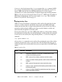
To create the auxiliary files, you set the AMPL option auxfiles to a string of letters denoting
the combination of auxiliary files you would like produced, and then use the write command
to create and save the auxiliary files along with the problem (*.nl) file. For example, the
command:
ampl: option auxfiles 'cr';
will cause the write command to create auxiliary files containing the names of the variables
(columns) and constraints (rows) as sent to the solver. The table below shows the types of
auxiliary files that can be created and the letter you use to request them via the AMPL option
auxfiles.
Table 3.1 Auxiliary Files
Letter
Extension
Description
a
.adj
adjustment to objective, for example, to compensate for fixed
variables eliminated by presolve
c
.col
AMPL names of the variables (columns) sent to the solver
f
.fix
names of variables fixed by presolve, and the values to which they
are fixed
r
.row
AMPL names of the constraints (rows) sent to the solver
s
.slc
names of “slack” constraints eliminated by presolve because they
can never be binding
u
.unv
names of variables dropped by presolve because they are never
used in the problem instance
IBM ILOG AMPL
V12.2 — USER’S GUIDE
21
Running Solvers Outside AMPL
With the write and solution commands, you can arrange to execute your solver outside
the AMPL session. You might want to do this if you receive an out of memory message
from your solver (not from AMPL itself): When the solver is invoked from within AMPL, a
fair amount of memory is already used for the AMPL Modeling System program code and
for data structures created by AMPL for its own use in memory. If you execute the solver
alone, it can use all available memory.
To run your solver separately, first use AMPL to create a problem file:
C:\> ampl
ampl: model steel.mod; data steel.dat;
ampl: write bsteel;
ampl: quit;
Then run your solver with a command like the one below (for CPLEX):
C:\> cplexamp steel -AMPL solver_options
In this example, the first argument steel matches the filename (after the initial letter b) in
the AMPL write command. The -AMPL argument tells the solver that it is receiving a
problem from AMPL. This may optionally be followed by any solver options you need for
the problem, using the same syntax used with the option solver_options command but
omitting the outer quotes, for example crash=1 relax. Assuming that the solver runs
successfully to completion, it will write a solution file; steel.sol in this case. You can
then restart AMPL and read in the results with the solution command, as outlined earlier:
C:\> ampl
ampl: model steel.mod; data steel.dat;
ampl: solution steel.sol;
Using MPS File Format
MPS file format, originally developed decades ago for IBM's Mathematical Programming
System, is a widely recognized format for linear and integer programming problems.
Although it is a standard supported by many solvers and modeling systems (including
AMPL), MPS file format is neither compact nor easy to read and understand; AMPL's
binary file format is a much more efficient way for modeling systems and solvers to
communicate. Also, MPS file format cannot be used for nonlinear problems, and not all
MPS-compatible solvers support exactly the same format, particularly for mixed integer
problems.
22
IBM ILOG AMPL
V12.2 — USER’S GUIDE
AMPL does have the ability to translate a model into MPS file format, as outlined below.
With this feature, you may be able to solve AMPL models with a solver that reads its
problem input in MPS file format. If you choose to use this feature, you will find AMPL's
ability to produce auxiliary files very useful, since these files can be used to relate the MPS
file format information to the sets, variables, constraints, and objectives defined in the
AMPL model. However, you will not be able to bring the solution—variable values, dual
values, and so on—back into AMPL; further work with the solution must be performed
outside of AMPL.
To translate your model into MPS file format, use the write command as outlined above
with m as the first letter of the filename. To illustrate, the command shown below creates a
file named steel.mps:
ampl: write msteel;
In most cases, you will need to run your solver separately to obtain the solution.
Note that the MPS format does not provide a way to distinguish between objective
maximization and minimization. However, CPLEX assumes that the objective is to be
minimized. (There is no standardization on this issue; other solvers may assume
maximization.) Thus, it is incumbent upon the user of the MPS format to ensure that the
objective sense in the AMPL model corresponds to the solver's interpretation.
Temporary Files Directory
If the TMPDIR option is not set, AMPL writes the problem and solution files and other
temporary files to the current directory. You can give a specific location for the temporary
files by setting option TMPDIR to a valid path. On a PC, you might use:
ampl: option TMPDIR 'D:\temp';
On a UNIX platform, a typical choice would be:
ampl: option TMPDIR '/tmp';
IBM ILOG AMPL
V12.2 — USER’S GUIDE
23
24
IBM ILOG AMPL
V12.2 — USER’S GUIDE
C
H
A
P
T
E
R
4
Customizing AMPL
Command Line Switches
Certain AMPL options normally set with the option command during an AMPL session
can also be set when AMPL is first invoked. This is done using a command line switch
consisting of a hyphen and a single letter, followed in some cases by a numeric or string
value. You will find these switches most useful when you have one or more model, data, or
run file that you want AMPL to process using different option settings at different times,
without actually editing the files themselves.
The table below summarizes the command line switches and their equivalent names when
set with the AMPL option command:
Table 4.1 AMPL Option Names for Command Line Switches
Switch
AMPL Option
Description
-Cn
Cautions n
n = 0: suppress caution messages
n = 1: report caution messages (default)
n = 2: treat cautions as errors
-en
eexit n
n > 0: abandon command after n errors
n < 0: abort AMPL after |n| errors
n = 0: report any number of errors
IBM ILOG AMPL
V12.2 — USER’S GUIDE
25
Switch
AMPL Option
Description
-f
funcwarn 1
do not treat unavailable functions of constant
arguments as variable
-P
presolve 0
turn off AMPL’s presolve phase
-S
substout 1
use “defining” equations to eliminate variables
-L
linelim 1
fully eliminate variables with linear “defining”
equations, so model is recognized as linear
-T
gentimes 1
show time to generate each model component
-t
times 1
show time taken in each model translation phase
-ostr
outopt str
set problem file format (b, g, m) and stub name;
to display more possibilities use -o?
-s
randseed ‘’
use current time for random number seed
-sn
randseed n
use n for random number seed
-v
version
display the AMPL software version number
If you type ampl -? at the shell prompt, AMPL will display a summary list of all the
command line switches. On some UNIX shells, ? is a special character, so you may need to
use "-?" with double quotation marks.
Persistent Option Settings
If you have many option settings or other commands that you would like performed each
time AMPL starts, you may create a text file containing these commands (in AMPL
language syntax). Then set the environment variable name OPTIONS_IN to the pathname of
this text file. For example, on a Windows PC, you should type:
C:\> set OPTIONS_IN=c:\amplinit.txt
If you are using a C shell on a UNIX machine you would type something like:
% setenv OPTIONS_IN ~ijr/amplinit.txt
AMPL reads the file referred to by OPTIONS_IN and executes any commands therein before
it reads any other files mentioned on the command line or prompts for any interactive
commands.
26
IBM ILOG AMPL
V12.2 — USER’S GUIDE
If you want AMPL to preserve all of your option settings from one session to the next, you
can cause AMPL to write the options into a text file named by setting the AMPL option
OPTIONS_INOUT:
ampl: option OPTIONS_INOUT 'c:\amplopt.txt';
Before exiting, AMPL writes a series of option commands to the file named by
OPTIONS_INOUT which, when read, will set all of the options to the values they had at the
end of the session. To use this text file, set the corresponding environment variable to the
same filename:
C:\> set OPTIONS_INOUT=c:\amplopt.txt
After you do this, AMPL will read and execute the commands in amplopt.txt when it
starts up. When you end a session, AMPL will write the current option settings - including
any changes you have made during the session - into this file, so that they will be preserved
for use in your next session.
If both the OPTIONS_IN and OPTIONS_INOUT environment variables are defined, the file
referred to by OPTIONS_IN will be processed first, then the file referred to by
OPTIONS_INOUT.
IBM ILOG AMPL
V12.2 — USER’S GUIDE
27
28
IBM ILOG AMPL
V12.2 — USER’S GUIDE
C
H
A
P
T
E
R
5
Using CPLEX with AMPL
Problems Handled by CPLEX
CPLEX is designed to solve linear programs as described in Chapters 1-8 and 15-16 of
AMPL: A Modeling Language for Mathematical Programming, 2nd. edition, as well as the
integer programs described in Chapter 20. Integer programs may be pure (all integer
variables) or mixed (some integer and some continuous variables); integer variables may be
binary (taking values 0 and 1 only) or may have more general lower and upper bounds.
For the network linear programs described in Chapter 15, CPLEX also incorporates an
especially fast network optimization algorithm.
The barrier algorithmic option to CPLEX, though originally designed to handle linear
programs, also allows the solution of a special class of nonlinear problems, namely,
quadratic programs (QPs), as described later in this section. However, CPLEX does not
solve general (non-QP) nonlinear programs. For instance, if you attempt to solve the
following nonlinear problem described in Chapter 18 of the AMPL book, CPLEX will
generate an error message:
ampl: model models\nltransd.mod;
ampl: data models\nltrans.dat;
ampl: option solver cplexamp;
ampl: solve;
at0.nl contains a nonlinear objective.
ampl:
IBM ILOG AMPL
V12.2 — USER’S GUIDE
29
This restriction applies if your model uses any function of variables that AMPL identifies as
"not linear" - even a function such as abs or min that shares some properties of linear
functions.
Piecewise-linear Programs
CPLEX does solve piecewise-linear programs, as described in Chapter 17, if AMPL
transforms them to problems that CPLEX solvers can handle. The transformation to a linear
program can be done if the following conditions are met:
◆ Any piecewise-linear term in a minimized objective must be convex, its slopes forming
an increasing sequence as in:
<<-1,1,3,5; -5, -1,0,1.5,3>> x[j]
◆ Any piecewise-linear term in a maximized objective must be concave, its slopes forming
a decreasing sequence as in:
<<1,3; 1.5,0.5,0.25>> x[j]
◆ Any piecewise-linear term in the constraints must be either convex and on the left-hand
side of a ≤ constraint (or equivalently, the right-hand side of a ≥ constraint), or else
concave and on the left-hand side of a ≥ constraint (the right-hand side of a ≤ constraint).
In all other cases, the transformation is to a mixed integer program. AMPL automatically
performs the appropriate conversion, sends the resulting linear or mixed integer program to
CPLEX, and converts the solution into user-defined variables. The conversion has the effect
of adding a variable to correspond to each linear piece; when the above rules are not
satisfied, additional integer variables and constraints must also be introduced.
Quadratic Programs
This user guide provides but a brief description of quadratic programming. In effect, it is
assumed that you are familiar with the area. Interested users may wish to consult a good
reference, such as Practical Optimization, by Gill, Murray and Wright (Academic Press,
1981) for more details.
A mathematical description of a quadratic program is given as:
minimize
subject to
1 T
- x Qx
2
T
+c x
Ax ~ b
l≤x≤u
where ~ represents ≤ , ≥ , or = operators.
In the above formula, Q represents a matrix of quadratic objective function coefficients. Its
diagonal elements Qii are the coefficients of the quadratic terms xi2. The nondiagonal
elements Qij and Qji are added together to be the coefficient of the term xixj.
30
IBM ILOG AMPL
V12.2 — USER’S GUIDE
The CPLEX linear programming algorithms incorporate an extension for quadratic
programming. For a problem to be solvable using this option, the following conditions must
hold:
1. All constraints must be linear.
2. The objective must be a sum of terms, each of which is either a linear expression or a
product of two linear expressions.
3. For any values of the variables (whether or not they satisfy the constraints), the quadratic
part of the objective must have a nonnegative value (if a minimization) or a nonpositive
value (if a maximization).
The last condition is known as positive semi-definiteness (for minimization) or negative
semi-definiteness (for maximization). CPLEX automatically recognizes nonlinear problems
that satisfy these conditions, and invokes the barrier algorithm to solve them. Nonlinear
problems of any other kind are rejected with an appropriate message.
Most CPLEX features applying to continuous LP models apply also to continuous QP
models; likewise most features applying to linear MIP models also apply to mixed-integer
QP models (MIQP). In cases where the nature of QP dictates different behavior from a
directive, usually the result is that the directive is ignored and default behavior remains in
effect. An example of this would be the dual directive to specify that CPLEX solves the
explicit dual formulation; for QP the default primal formulation will be used anyway. In
almost every case, such differences will result in best performance and will require no user
intervention.
Quadratic Constraints
A model containing one or more quadratic constraints of the form
ax + x Qx ≤ r
T
is called a Quadratically Constrained Program (QCP), and can be solved using the CPLEX
barrier algorithm. Linear constraints may also be present in a QCP, and a (positive semidefinite) quadratic term in the objective function is permitted. If discrete variables are
present, then the model is termed Mixed Integer QCP, or MIQCP.
The Q matrix for each quadratic constraint must be positive semi-definite, just as for a
quadratic objective function, to ensure that the feasible space remains convex.
Most of the comments regarding CPLEX features, in section Quadratic Programs above,
also pertain to QCP, with the additional observation that only the barrier optimizer applies to
continuous models that have any quadratic constraints, and therefore barrier is also the only
choice for subproblem solution of MIQCP models.
IBM ILOG AMPL
V12.2 — USER’S GUIDE
31
Specifying CPLEX Directives
In many instances, you can successfully apply CPLEX by simply specifying a model and
data, setting the solver option to cplex, and typing solve. For larger linear programs and
especially the more difficult integer programs, however, you may need to pass specific
options (also referred to as directives) to CPLEX to obtain the desired results.
To give directives to CPLEX, you must first assign an appropriate character string to the
AMPL option called cplex_options. When CPLEX is invoked by solve, it breaks this
string into a series of individual directives. Here is an example:
ampl: model diet.mod;
ampl: data diet.dat;
ampl: option solver cplexamp;
ampl: option cplex_options 'crash=0 dual \
ampl?
feasibility=1.0e-8 scale=1 \
ampl?
lpiterlim=100';
ampl: solve;
CPLEX 11.0.0: crash 0
dual
feasibility 1e-08
scale 1
lpiterlim 100
CPLEX 11.0.0: optimal solution; objective 88.2
1 iterations (0 in phase I)
CPLEX confirms each directive; it will display an error message if it encounters one that it
does not recognize.
CPLEX directives consist of an identifier alone, or an identifier followed by an = sign and a
value; a space may be used as a separator in place of the =.
You may store any number of concatenated directives in cplex_options. The example
above shows how to type all the directives in one long string, using the \ character to
indicate that the string continues on the next line. Alternatively, you can list several strings,
which AMPL will automatically concatenate:
ampl: option cplex_options 'crash=0 dual'
ampl?
' feasibility=1.0e-8 scale=1'
ampl?
' lpiterlim=100';
In this form, you must take care to supply the space that goes between the directives; here we
have put it before feasibility and iterations.
If you have specified the directives above, and then want to try setting, say, optimality to
1.0e-8 and changing crash to 1, you could use:
ampl: option cplex_options
ampl?
'optimality=1.0e-8 crash=1';
However, this will replace the previous cplex_options string. The other previously
specified directives such as feasibility and iterations will revert to their default values.
32
IBM ILOG AMPL
V12.2 — USER’S GUIDE
CPLEX supplies a default value for every directive not explicitly specified; defaults are
indicated in the discussion below.
To append new directives to cplex_options, use this form:
ampl: option cplex_options $cplex_options
ampl?
' optimality=1.0e-8 crash=1';
A $ in front of an option name denotes the current value of that option, so this statement just
appends more directives to the current directive string. As a result the string contains two
directives for crash, but the new one overrides the earlier one.
Directives for Handling Infeasible Problems
The following directives are useful when CPLEX finds that your problem is infeasible.
Setting these options directs CPLEX to take additional steps when solve is invoked and the
problem is infeasible. The feasopt and feasoptobj directives tell CPLEX to relax
constraints and bounds to find a feasible solution. The iisind directive tells CPLEX to try
to refine the conflict among the constraints and bounds to a smaller set of constraints and
bounds. These directives can also be applied to integer programs.
conflictdisplay=i
default 1
This directive controls the amount of output during conflict refinement. Set i=0 for no
output, i=1 for summary output and i=2 for a detailed display.
feasopt=i
default 0
Whether to find a feasible point for a relaxed problem when the problem is infeasible. With
the default setting of 0, no feasible point is found. Set i=1 to find a feasible point and i=2 to
find an optimal feasible point among all those that require only as much relaxation as is
needed to find the first feasible point.
feasoptobj=i
default 1
This directive sets the objective to use in measuring minimality of a relaxation. Set i=1 for
minimizing the sum of the relaxations of constraints and bounds. Set i=2 for minimizing the
number of constraints and bounds that must be relaxed. Set i=3 to minimize the sum of
squares of the required relaxations of constraints and bounds.
iisfind=i
(default 0)
When i=1 for an infeasible problem, CPLEX returns an irreducible infeasible subset (IIS) of
the constraints and variable bounds. By definition, members of an IIS have no feasible
solution, but dropping any one of them permits a solution to be found to the remaining ones.
Clearly, knowing the composition of an IIS can help localize the source of the infeasibility.
When iisfind is used, CPLEX uses the .iis suffix to specify which variables and
constraints are in the IIS, as explained in Diagnosing Infeasibilities on page 81.
IBM ILOG AMPL
V12.2 — USER’S GUIDE
33
Directive for Tuning
CPLEX can try various values for algorithmic directives to find a set of values that will
reduce solution time. The directives below are used to control the tuning algorithm. The
algorithm progresses by trying different sets of values in trial runs.
tunefile=f1
tunefileprm=f2
These directives tell CPLEX to do tuning and to write the results to file f1 using AMPL
directive names or to file f2 in CPLEX PRM format. The tuning algorithm can take up to six
to ten times longer than a regular solve invocation, but the results may save time in future
runs.
pretunefile=f1
pretunefileprm=f2
These directives tell CPLEX to write out the current non-default directive settings before
starting tuning. The files may be used to return to the pre-tuning settings, since CPLEX will
change all settings to the tuned values as part of the tuning algorithm. The file f1 uses
AMPL directive names and the file f2 is written in CPLEX PRM format. The
pretunefileprm (f2) file may contain some CPLEX display settings which are not included
in the pretunefile (f1) form of the file.
paramfile=f1
paramfileprm=f2
These directives are used to import the settings contained in either the f1 or f2 files. The f1
file uses AMPL directive names and the f2 file is a CPLEX PRM file.
tunefix=l
This directive tells CPLEX which parameters to keep fixed during the tuning algorithm. The
tuning algorithm starts with all parameters at their default values, except those specified in l.
l is a list of directives and values, either enclosed in single or double quotes or separated by
commas with no white space if more than one. The list l is combined with any settings from
the tunefixfile directive. Example:
tunefix "mipgap=0”
tunefixfile=f
The name of a file with AMPL directives which CPLEX should leave fixed during the tuning
algorithm. The tuning algorithm starts with all parameters at their default values, except
those specified in f. The set of parameters in f is combined with any settings from the
tunefix directive.
tunedisplay=i
(default 1)
This directive controls the amount of output from the tuning algorithm. No output is
produced when i=0. A minimal amount is produced when i=1. The parameters being tried
are printed when i=2, and full logs are printed when i=3.
34
IBM ILOG AMPL
V12.2 — USER’S GUIDE
tunerepeat=i
(default 1)
CPLEX can tune on several variations of the problem. The variations are obtained by
permuting the rows and columns of the problem. Tuning on several variations may give
more robust tuning results.
tunetime=r
(default 10000)
This directive limits the time per tuning trial. This directive is meaningful only if r is less
than the value of the time directive.
IBM ILOG AMPL
V12.2 — USER’S GUIDE
35
36
IBM ILOG AMPL
V12.2 — USER’S GUIDE
C
H
A
P
T
E
R
6
Using CPLEX for Continuous Optimization
CPLEX Algorithms for Continuous Optimization
For problems with linear constraints, CPLEX employs either a simplex method or a barrier
method to solve the problem. Refer to a linear programming textbook for more information
on these algorithms. Four distinct methods of optimization are incorporated in the CPLEX
package:
◆ A primal simplex algorithm that first finds a solution feasible in the constraints (Phase I),
then iterates toward optimality (Phase II).
◆ A dual simplex algorithm that first finds a solution satisfying the optimality conditions
(Phase I), then iterates toward feasibility (Phase II).
◆ A network primal simplex algorithm that uses logic and data structures tailored to the
class of pure network linear programs.
◆ A primal-dual barrier (or interior-point) algorithm that simultaneously iterates toward
feasibility and optimality, optionally followed by a primal or dual crossover routine that
produces a basic optimal solution (see below).
CPLEX normally chooses one of these algorithms for you, but you can override its choice by
the directives described below.
IBM ILOG AMPL
V12.2 — USER’S GUIDE
37
The default algorithm when your computer has more than one processor or core and the
threads and parallelmode directives are at their default values is a deterministic variant
of the concurrentopt algorithm which is described below.
For problems with quadratic constraints, only the barrier method is used and there is no
crossover algorithm.
The simplex algorithm maintains a subset of basic variables (or, a basis) equal in size to the
number of constraints. A basic solution is obtained by solving for the basic variables, when
the remaining nonbasic variables are fixed at appropriate bounds.
Each iteration of the algorithm picks a new basic variable from among the nonbasic ones,
steps to a new basic solution, and drops some basic variable at a bound.
The coefficients of the variables form a constraint matrix, and the coefficients of the basic
variables form a nonsingular square submatrix called the basis matrix. At each iteration, the
simplex algorithm must solve certain linear systems involving the basis matrix. For this
purpose CPLEX maintains a factorization of the basis matrix, which is updated during most
iterations, and is occasionally recomputed.
The sparsity of a matrix is the proportion of its elements that are not zero. The constraint
matrix, basis matrix and factorization are said to be relatively sparse or dense according to
their proportion of nonzeros. Most linear programs of practical interest have many zeros in
all the relevant matrices, and the larger ones tend also to be the sparser.
The amount of RAM memory required by CPLEX grows with the size of the linear program,
which is a function of the numbers of variables and constraints and the sparsity of the
coefficient matrix. The factorization of the basis matrix also requires an allocation of
memory; the amount is problem-specific, depending on the sparsity of the factorization.
When memory is limited, CPLEX automatically makes adjustments that reduce its
requirements, but that usually also reduce its optimization speed.
The CPLEX directives in the following subsections apply to the solution of linear programs,
including network linear programs. The letters i and r denote integer and real values,
respectively.
Directives for Problem and Algorithm Selection
CPLEX consults several directives to decide how to set up and solve a linear program that it
receives. The default is to apply the dual simplex method to the linear program as given,
substituting the network variant if the AMPL model contains node and arc declarations. The
following discussion indicates situations in which you should consider experimenting with
alternatives.
38
IBM ILOG AMPL
V12.2 — USER’S GUIDE
dualthresh=i
primal
dual
(default 32000)
Every linear program has an equivalent "opposite" linear program; the original is
customarily referred to as the primal LP, and the equivalent as the dual. For each variable
and each constraint in the primal there are a corresponding constraint and variable,
respectively, in the dual. Thus when the number of constraints is much larger than the
number of variables in the primal, the dual has a much smaller basis matrix, and CPLEX
may be able to solve it more efficiently.
The primal and dual directives instruct CPLEX to set up the primal or the dual formulation,
respectively. The dualthresh directive makes a choice: the dual LP if the number of
constraints exceeds the number of variables by more than i, and the primal LP otherwise.
autoopt
dualopt
baropt
primalopt
siftopt
concurrentopt
The autoopt directive instructs CPLEX to select an appropriate algorithm to solve the
problem. You can specify a particular algorithm by the dualopt, baropt, and primalopt
directives, which invoke dual simplex, barrier, and primal simplex methods respectively. The
autoopt directive will most frequently select the dual simplex method. The two simplex
variants use similar basis matrices but employ opposite strategies in constructing a path to
the optimum. Any of the algorithms can be applied regardless of whether the primal or the
dual LP is set up as explained above; in general the six combinations of primalopt/
dualopt/baropt and primal/dual perform differently.
Consider trying the barrier method or the primal simplex method if CPLEX’s dual simplex
method reports problems in its display or if you simply wish to determine whether another
algorithm will be faster. Few linear programs exhibit poor numerical performance in both
the primal and the dual algorithms. In general the barrier method tends to work well when
the product of the constraint matrix and its transpose remains sparse.
The siftopt directive instructs CPLEX to use a sifting method that solves a sequence of
LP subproblems, eventually converging to an optimal solution for the full original model.
Sifting is especially applicable to models with many more columns than rows when the
eventual solution is likely to have a majority of variables placed at their lower bounds.
The concurrentopt directive instructs CPLEX to make use of multiple processors on your
computer by launching concurrent threads to solve your model in parallel. The
concurrentopt algorithm has two modes, depending on the setting of the parallelmode
directive. In the opportunistic mode, the first thread uses dual simplex, a second thread uses
barrier, a third thread (if your computer has that many processors) uses primal simplex, and
any additional processors are added to making barrier parallel. On a machine with enough
memory, this strategy will result in a solution being returned by the fastest of the available
IBM ILOG AMPL
V12.2 — USER’S GUIDE
39
algorithms on each problem, eliminating the need to choose a single optimizer for all
purposes. In the deterministic mode, one thread will be used for dual simplex and if
available, a second thread will be used for barrier with crossover.
memoryemphasis=i
workfilelim=r
workfiledir=f
(default 0)
(default 128)
This directive lets you indicate to CPLEX that it should conserve memory where possible.
When you set this parameter to its nondefault value of 1, CPLEX will choose tactics, such as
data compression or disk storage, for some of the data computed by the simplex, barrier and
MIP optimizers. Of course, conserving memory may impact performance in some models.
Also, while solution information will be available after optimization, certain computations
that require a basis that has been factored (for example, for the computation of the basis
condition number) may be unavailable. The workfilelim directive specifies the maximum
amount of RAM that may be used for the Cholesky factorization of the barrier optimizer
before files are used for the remainder of memory needs. The default is 128, which means
CPLEX will use 128 megabytes of RAM before using disk space. These temporary barrier
files are created in the directory specified by the value of the workfiledir directive. If no
value is specified, the directory specified by the TMPDIR (on UNIX) or TMP (on Windows)
environment variable is used. If TMPDIR or TMP are not set either, the current working
directory is used. Temporary barrier files are deleted automatically when CPLEX terminates
normally.
threads=i
(default 0)
This directive specifies a global thread limit, that is, a default thread count for the parallel
MIP, parallel barrier, and concurrentopt optimizers. The value 0 tells CPLEX to use as
many threads as are allowed by the license when the parallelmode directive is -1. A
value of 0 when parallelmode is 0 or -1 tells CPLEX to use as many threads as possible
subject to maintaining a deterministic algorithm. A positive value for i specifies that i
threads should be used.
netopt=i
(default 1)
CPLEX incorporates an optional heuristic procedure that looks for "pure network"
constraints in your linear program. If this procedure finds sufficiently many such constraints,
CPLEX applies its fast network simplex algorithm to them. Then, if there are also nonnetwork constraints, CPLEX uses the network solution as a start for solving the whole LP by
the general primal or dual simplex algorithm, whichever you have chosen.
The default value of i=1 invokes the network-identification procedure if and only if your
model uses node and arc declarations, and CPLEX sets up the primal formulation as
discussed above. Setting i=0 suppresses the procedure, while i=2 requests its use in all
cases. You can have CPLEX display the number of network nodes (constraints) and arcs
(variables) that it has extracted, by setting the prestats directive (described with the
preprocessing options below) to 1.
CPLEX's network simplex algorithm can achieve dramatic reductions in optimization time
for "pure" network linear programs defined entirely in terms of node and arc declarations.
40
IBM ILOG AMPL
V12.2 — USER’S GUIDE
(For a pure network LP, every arc declaration must contain at most one from and one to
phrase, and these phrases may not specify optional coefficients.) In the case of linear
programs that are mostly defined in terms of node and arc declarations, but that have some
"side" constraints defined by subject to declarations, the benefit is highly dependent on
problem structure; it is best to try experimenting with both i=0 and i=1.
parallelmode=i
(default 0)
This directive sets the type of parallelism used by CPLEX. Multiple runs of the same
problem with the same settings will get identical solution paths with deterministic mode, but
not with opportunistic mode. Opportunistic mode can be faster than deterministic mode, due
to less synchronization among the threads. The default (automatic) setting allows CPLEX to
choose between deterministic and opportunistic mode depending on the threads directive.
If the threads directive is set to its automatic setting (the default), CPLEX chooses
deterministic mode. If the threads directive is set to one, CPLEX runs sequentially in
deterministic mode in a single thread. Otherwise, if the threads directive is set to a value
greater than one, CPLEX chooses opportunistic mode. The value i=1 is used to set
deterministic mode and the value i=-1 is used to set opportunistic mode.
relax
This directive instructs CPLEX to ignore any integrality restrictions on the variables. The
resulting linear program is solved by whatever algorithm the above directives specify.
maximize
minimize
While AMPL completely specifies the problem and its objective sense, it is possible to
change the objective sense after specifying the model. The two directives instruct CPLEX to
set the objective sense to be minimize or maximize, respectively.
Directives for Preprocessing
Prior to applying any simplex algorithm, CPLEX modifies the linear program and initial
basis in ways that tend to reduce the number of iterations required. The following directives
select and control these preprocessing features.
aggregate=i1
(default 1)
aggfill=i2
(default 10)
When i1 is left at its default value of 1, CPLEX looks for constraints that (possibly after
some rearrangement) define a variable x in terms of other variables:
◆ two-variable constraints of the form x = y + b;
◆ constraints of the form x = Σj yj, where x appears in less than i2 other constraints.
Under certain conditions, both x and its defining equation can be eliminated from the linear
program by substitution. In CPLEX's terminology, each such elimination is an aggregation
of the linear program. When i1 is -1, CPLEX decides how many passes to perform. Set i1
IBM ILOG AMPL
V12.2 — USER’S GUIDE
41
to 0 to prevent any such aggregations. Set i1 to a positive integer to specify the precise
number of passes.
Aggregation can yield a substantial reduction in the size of some linear programs, such as
network flow LPs in which many nodes have only one incoming or one outgoing arc. If i2
> 2, however, aggregation may also increase the number of nonzero constraint coefficients,
resulting in more work at each simplex iteration. The default setting of i2=10 usually makes
a good tradeoff between reduction in size and increase in nonzeros, but you may want to
experiment with lower values if CPLEX reports that many aggregations have been made. If
CPLEX consistently reports that no aggregations can be performed, on the other hand, you
can set i1 to 0 to turn off the aggregation routine and save memory and processing time.
To request a report of the number of aggregations, see the prestats directive later in this
section.
dependency=i
(default -1)
By default (i=-1), CPLEX chooses automatically when to use dependency checking. This
parameter offers several settings that make it possible for a user to control dependency
checking more precisely. Table 6.1 shows you the possible settings of the parameter that
controls dependency checking, and indicates their effects.
Table 6.1 Settings for the dependency Directive
Setting
Effect
-1 (default) automatic: let CPLEX choose when to use dependency checking
0
turn off dependency checking
1
turn on only at the beginning of preprocessing
2
turn on only at the end of preprocessing
3
turn on at the beginning and at the end of preprocessing
predual=i
(default 0)
By default, after presolving the problem CPLEX decides whether to solve the primal or dual
problem based on which problem it determines it can solve faster. Setting i=1 explicitly
instructs CPLEX to solve the dual problem, while setting it to -1 explicitly instructs CPLEX
to solve the primal problem.
Regardless of the problem CPLEX solves internally, it still reports primal solution values.
This is often a useful technique for problems with more constraints than variables.
prereduce=i
(default 3)
This directive determines whether primal reductions, dual reductions or both are performed
during preprocessing. By default, CPLEX performs both. Set this directive to 0 to prevent all
reductions, 1 to only perform primal reductions, and 2 to only perform dual reductions.
42
IBM ILOG AMPL
V12.2 — USER’S GUIDE
While the default usually suffices, performing only one kind or the other may be useful
when diagnosing infeasibility or unboundedness.
presolve=i
(default 1)
Prior to invoking any simplex algorithm, CPLEX applies transformations that reduce the
size of the linear program without changing its optimal solution. In this presolve phase,
constraints that involve only one non-fixed variable are removed; either the variable is fixed
and also dropped (for an equality constraint) or a simple bound for the variable is recorded
(for an inequality). Each inequality constraint is subjected to a simple test to determine if
there exists any setting of the variables (within their bounds) that can violate it; if not, it is
dropped as nonconstraining. Further iterative tests attempt to tighten the bounds on primal
and dual variables, possibly causing additional variables to be fixed, and additional
constraints to be dropped.
AMPL's presolve phase, as described in Section 14.1 of the AMPL book, also performs
many (but not all) of these transformations. To see how many variables and constraints are
eliminated by AMPL's presolve, set option show_stats to 1. To suppress AMPL's
presolver, so that all presolving is done in CPLEX, set option presolve to 0.
CPLEX's presolve can be suppressed by changing i to 0 from its default of 1. In rare cases
the presolved linear program, although smaller, is actually harder to solve. Thus if CPLEX
reports that many variables and constraints have been eliminated by presolve, you may want
to compare runs with and without presolve. On the other hand, if CPLEX consistently
reports that presolve eliminates no variables or constraints, you can save a little processing
time by turning presolve off.
To request a report of the number of eliminations performed by presolve, see the prestats
directive below.
prestats=i
(default 0)
When this directive is changed to 1 from its default of 0, CPLEX reports on the activity of
the aggregation and presolve routines:
Presolve eliminated 1645 rows and 2715 columns in 3 passes.
Aggregator did 22 substitutions.
Presolve Time =
1.70 sec.
During the development of a large or complex model, it is a good idea to monitor this report,
and to turn on its AMPL counterpart by setting option show_stats to 1. An unexpectedly
large number of eliminated variables or constraints may indicate that the formulation is in
error or can be substantially simplified.
scale=i
(default 0)
This directive governs the scaling of the coefficient matrix. The default value of i=0
implements an equilibration scaling method, which is generally very effective. You can turn
off the default scaling by setting i=-1. A value of 1 invokes a modified, more aggressive
scaling method that can produce improvements on some problems. Since CPLEX has
internal logic that determines when it need not scale a problem, setting the scale directive
to -1 rarely improves performance.
IBM ILOG AMPL
V12.2 — USER’S GUIDE
43
Directives for Controlling the Simplex Algorithm
Several key strategies of the primal and dual simplex algorithms can be changed through
CPLEX directives. If you are repeatedly solving a class of linear programs that requires
substantial computer time, experimentation with alternative strategies can be worthwhile.
advance=i
(default 0)
By default (i=0), the advanced basis indicator is off. You can set it according to Table 6.2.
Table 6.2 Settings for the advance Directive
Setting
Effect
0
This is the default value. The advanced basis indicator is off.
1
The advanced indicator is on; CPLEX uses an advanced basis supplied by the
user. Preprocessing is skipped.
2
The advanced indicator is on and CPLEX will crush an advanced basis or
starting vector supplied by the user.
If this parameter is set to 1 or 2, CPLEX uses advanced starting information when
optimization is initiated.
◆ If you anticipate the advanced basis to be a close match for your problem, so that
relatively few iterations will be needed, or if you are unsure, then setting 1 is a good
choice because it avoids some overhead processing.
◆ If you anticipate that the simplex optimizer will require many iterations even with the
advanced basis, or if the model is large and preprocessing typically removes much from
the model, then setting 2 may yield a faster solution by giving you the advantages of
preprocessing. However, in such cases, you might also consider not using the advanced
basis, by setting this parameter to 0 instead, on the grounds that the basis may not be
giving you a helpful starting point after all.
Setting 2 may also be effective for MIPs in which the percentage of integer constraints is
low. It may also reduce the solution time of fixed MIPs.
crash=i
(default 1)
This directive governs CPLEX's procedure for choosing an initial basis, except when the
basis is read from a file as specified by the directive readbasis described below. A value of
i=0 causes the objective to be ignored in choosing the basis, whereas values of -1 and 1
select two different heuristics for taking the objective into account. The best setting for your
purposes will depend on the specific characteristics of the linear programs you are solving,
and must be determined through experimentation.
pgradient=i
(default 0)
This directive governs the primal simplex algorithm's choice of a "pricing" procedure that
determines which variable is selected to enter the basis at each iteration. Your choice is
44
IBM ILOG AMPL
V12.2 — USER’S GUIDE
likely to make a substantial difference to the tradeoff between computational time per
iteration and the number of iterations. As a rule of thumb, if the number of iterations to solve
your linear program exceeds three times the number of constraints, you should consider
experimenting with alternative pricing procedures.
The recognized values of i are as follows:
Table 6.3 Settings for the pgradient Directive
-1
Reduced-cost pricing
0
Hybrid reduced-cost/devex pricing
1
Devex pricing
2
Steepest-edge pricing
3
Steepest-edge pricing in slack pace
4
Full pricing
The "reduced cost" procedures are sophisticated versions of the pricing rules most often
described in textbooks. The "devex" and "steepest edge" alternatives employ more elaborate
computations, which can better predict the improvement to the objective offered by each
candidate variable for entering the basis.
Compared to the default of i=0, the less compute-intensive reduced-cost pricing (i= -1)
may be preferred if your problems are small or easy, or are unusually dense—say, 20 to 30
nonzeros per column. Conversely, if you have more difficult problems which take many
iterations to complete Phase I, consider using devex pricing (i=1). Each iteration may
consume more time, but the lower number of total iterations may lead to a substantial overall
reduction in time. Do not use devex pricing if your problem has many variables and
relatively few constraints, however, as the number of calculations required per iteration in
this situation is usually too large to afford any advantage.
If devex pricing helps, you may wish to try steepest-edge pricing (i=2). This alternative
incurs a substantial initialization cost, and is computationally the most expensive per
iteration, but may dramatically reduce the number of iterations so as to produce the best
results on exceptionally difficult problems. The variant using slack norms (i=3) is a
compromise that sidesteps the initialization cost; it is most likely to be advantageous for
relatively easy problems that have a low number of iterations or time per iteration.
Full reduced-cost pricing (i=4) is a variant that computes a reduced cost for every variable,
and selects as entering variable one having most negative reduced cost (or most positive, as
appropriate). Compared to CPLEX's standard reduced-cost pricing (i=-1), full reduced-cost
pricing takes more time per iteration, but in rare cases reduces the number of iterations more
than enough to compensate. This alternative is supplied mainly for completeness, as it is
proposed in many textbook discussions of the simplex algorithm.
dgradient=i
(default 0)
This directive governs the dual simplex algorithm's choice of a "pricing" procedure that
determines which variable is selected to leave the basis at each iteration. Your choice is
IBM ILOG AMPL
V12.2 — USER’S GUIDE
45
likely to make a substantial difference to the tradeoff between computational time per
iteration and the number of iterations. As a rule of thumb, if the number of iterations to solve
your linear program exceeds three times the number of constraints, you should consider
experimenting with alternative pricing procedures.
The dual pricing indicator allows you to indicate devex pricing. Table 6.4 lists the valid
settings for this directive.
Table 6.4 Dual Pricing Indicator dgradient
Setting Effect
0
Let CPLEX determine automatically
1
Standard dual pricing
2
Steepest-edge pricing
3
Steepest-edge pricing in slack space
4
Steepest-edge pricing, unit initial norms
5
Devex pricing
These settings can be further described as follows:
◆ The default value (i=0) lets CPLEX choose a dual pricing procedure through an internal
heuristic based on problem characteristics.
◆ Standard dual pricing (i=1), described in many textbooks, selects as leaving variable one
that is farthest outside its bounds.
◆ The three "steepest edge" alternatives employ more elaborate computations, which can
better predict the improvement to the objective offered by each candidate for leaving
variable. Steepest-edge pricing involves an extra initialization cost, but its extra cost per
iteration is much less in the dual simplex algorithm than in the primal. Thus if you find
that your problems solve faster using the dual simplex, you should consider
experimenting with the steepest-edge procedures.
●
The standard procedure (i=2) and the variant "in slack space" (i=3) have similar
computational costs; often their overall performance is similar as well, though one or
the other can be advantageous for particular applications.
●
The variant using "unit initial norms" (i=4) is a compromise that sidesteps the
initialization cost; it is most likely to be advantageous for relatively easy problems
that have a low number of iterations or time per iteration.
pricing=i
(default 0)
To promote efficiency, when using reduced-cost pricing in primal simplex, CPLEX
considers only a subset of the nonbasic variables as candidates to enter the basis. The default
of i=0 selects a heuristic that dynamically determines the size of the candidate list, taking
46
IBM ILOG AMPL
V12.2 — USER’S GUIDE
problem dimensions into account. You can manually set the size of this list to i>0, but only
very rarely will this improve performance.
refactor=i
(default 0)
This directive specifies the number of iterations between refactorizations of the basis matrix.
At the default setting of i=0, CPLEX automatically calculates a refactorization frequency by
a heuristic formula. You can determine the frequency that CPLEX is using by setting the
display directive (described below) to 1.
Since each update to the factorization uses more memory, CPLEX may reduce the
factorization frequency if memory is low. In extreme cases, the basis may have to be
refactored every few iterations and the algorithm will be very slow.
Given adequate memory, CPLEX's performance is relatively insensitive to changes in
refactorization frequency. For a few extremely large, difficult problems you may be able to
improve performance by reducing i from the value that CPLEX chooses.
netfind=i
(default 1)
This directives governs the method used by the CPLEX network optimizer to extract a
network from the linear program. The value of i influences the size of the network
extracted, potentially reducing optimization time. The default value (i=1) extracts only the
natural network from the problem. CPLEX then invokes its network simplex method on the
extracted network. In some cases, CPLEX can extract a larger network by multiplying rows
by -1 (reflection scaling) and rescaling constraints and variables so that more matrix
coefficients are plus or minus 1. Setting the netfind directive to 2 enables reflection scaling
only, while setting it to 3 allows reflection scaling and general scaling.
Directives for Controlling the Barrier Algorithm
Several key strategies of the barrier algorithm can be changed through CPLEX directives. If
you are repeatedly solving a class of linear programs that requires substantial computer time,
experimentation with alternative strategies can be worthwhile.
baralg=i1
(default 0)
The automatically determined choice of barrier algorithm (i1=0) is usually the fastest.
However, on primal- or dual-infeasible problems, the infeasibility-estimate start algorithm
(i1=1) or the infeasibility-constant start algorithm (i1=2) may improve numerical stability,
possibly at the cost of speed. Setting i1=3 selects the standard barrier algorithm.
bargrowth=r
(default 1e+12)
This directive is used to detect unbounded optimal faces. At higher values, the barrier
algorithm will be less likely to conclude that the problem has an unbounded optimal face,
but more likely to have numerical difficulties if the problem does have an unbounded face.
Any positive number is acceptable input.
IBM ILOG AMPL
V12.2 — USER’S GUIDE
47
barcorr=i
(default -1)
CPLEX may perform centering corrections if it encounters numerical difficulties during the
barrier method optimization. By default (i=-1) the barrier solver automatically computes an
estimate for the maximum number of centering corrections done at each iteration. If the
automatic estimate is computed to be 0, setting the value to a positive integer may improve
the numerical stability of the algorithm, probably at the expense of computation time.
barobjrange=r
(default 1e+20)
This directive sets the maximum absolute value of the objective function. CPLEX's barrier
algorithm looks at this value to detect unbounded problems. Any positive value is acceptable
input. However, care should be taken to avoid choosing a value so small that CPLEX will
conclude a problem is unbounded when it is not.
barstart=i
(default 1)
This directive controls the starting point CPLEX uses to initiate the barrier method. The
default setting of 1 will suffice for most problems. Consider other values (2, 3, and 4) if the
barrier method appears to converge slowly, or when the predual directive is specified.
comptol=r
(default 1e-8)
This directive specifies the complementarity tolerance used by the barrier algorithm to test
convergence. The barrier algorithm will terminate with an optimal solution if the relative
complementarity is smaller than this value. Any positive number larger than 1e-10 is
acceptable input.
crossover=i
(default 1)
On a linear problem, by default (i=1) CPLEX initiates the "crossover" algorithm to convert
the barrier solution to a basic (or vertex) solution using a primal simplex-like method. If
i=2, a dual simplex-like method is used for the crossover. The crossover algorithm can be
turned off by setting i=0.
densecol=i
(default 0)
CPLEX uses this directive to distinguish dense columns in the constraint matrix. Because
barrier algorithm performance can improve dramatically if dense columns are treated
separately, changing this value may improve optimization time. Columns with more
nonzeros than this setting are considered to be dense. If left at the default value, CPLEX will
automatically determine a value, considering factors such as the size of the problem. Any
nonnegative integer is acceptable input.
ordering=i
(default 0)
This directive selects the method used to permute the rows of the constraint matrix in order
to reduce fill in the Cholesky factor. There is a trade-off between ordering speed and sparsity
of the Cholesky factor. The automatic default setting usually chooses the best ordering for
the problem.
The approximate minimum degree (AMD) algorithm (i=1) balances speed and fill. The
approximate minimum fill (AMF) algorithm (i=2) usually generates slightly better
orderings than AMD, at the cost of more ordering run-time. The nested dissection (ND)
algorithm, triggered by using i=3 sometimes reduces Barrier run-time dramatically—ten48
IBM ILOG AMPL
V12.2 — USER’S GUIDE
fold reductions have been observed for some problems. This option sometimes produces
worse orderings, though, and it requires much more ordering run-time.
qcpconvergetol
(default 1e-7)
This directive sets the tolerance on complementarity for convergence in quadraticallyconstrained problems (QCP). The barrier algorithm terminates with an optimal solution if
the relative complementarity is smaller than this value.
Changing this tolerance to a smaller value may result in greater numerical precision of the
solution, but also increases the chance of a convergence failure in the algorithm and
consequently may result in no solution at all. Therefore, caution is advised in deviating from
the default setting.
For LPs and QPs, (that is, when all the constraints are linear) see the comptol directive.
Directives for Improving Stability
CPLEX is highly robust and has been designed to avoid problems such as degenerate stalling
and numerical inaccuracy that can occur in the simplex algorithm. However, some linear
programs can benefit from adjustments to the following directives if difficulties are
encountered.
numericalemphasis=i
(default 0)
This directive lets you indicate to CPLEX that it should emphasize precision in numerically
difficult or unstable problems, with consequent performance trade-offs in time and memory.
When set to its nondefault value of 1, CPLEX will choose tactics that emphasize numerical
stability. Try setting this directive before trying any of the other settings in this section.
doperturb=i1
perturbation=r
perturblimit=i2
(default 0)
(default 1.0e-6)
(default 0)
The simplex algorithm tends to make very slow progress when it encounters solutions that
are highly degenerate (in the sense of having many basic variables lying at one of their
bounds, rather than between them). When CPLEX detects degenerate stalling, it
automatically introduces a perturbation that expands the bounds on every variable by a small
amount, thereby creating a different but closely related problem. Generally, CPLEX can
make faster progress on this less constrained problem; once optimality is indicated, the
perturbation is removed by resetting the bounds to their original values.
The value of r determines the size of the perturbation. If you receive messages from CPLEX
indicating that the linear program has been perturbed more than once, r is probably too
large; reduce it to a level where only one perturbation is required.
The default doperturb value of i1=0 selects CPLEX's automatic perturbation strategy. If
an automatic perturbation occurs early in the solution process, consider setting i1=1 to
select perturbation at the outset. This alternative will save the time of first allowing the
IBM ILOG AMPL
V12.2 — USER’S GUIDE
49
optimization to stall before activating the perturbation mechanism, but is useful only rarely,
for extremely degenerate problems.
The perturblimit parameter governs the number of stalled iterations CPLEX allows
before perturbing the problem. The default value of i2=0 causes CPLEX to determine this
number based on the characteristics of the particular problem being solved. Setting i2 to a
positive integer value identifies a specific number of stalled iterations to tolerate before
perturbing the problem.
feasibility=r1
markowitz=r2
optimality=r3
(default 1.0e-6)
(default 0.01)
(default 1.0e-6)
If a problem is making slow progress through Phase I, or repeatedly becomes infeasible
during Phase II, numerical difficulties have arisen. Adjusting the algorithmic tolerances
controlled by these directives may help. Decreasing the feasibility tolerance, increasing the
optimality tolerance and/or increasing the Markowitz tolerance will typically improve
numerical behavior.
The feasibility tolerance r1>0 specifies the degree to which a linear program's basic
variables may violate their bounds. You may wish to lower r1 after finding an optimal
solution if there is any doubt that the solution is truly optimal; but if it is set too low, CPLEX
may falsely conclude that the problem has no feasible solution. Valid values for r1 lie
between 1e-9 and 0.1.
The Markowitz threshold r2<1 influences the order in which variables are eliminated during
basis factorization. Increasing r2 may yield a more accurate factorization, and consequently
more accurate computations during iterations of the simplex algorithm. Too large a value
may produce an inefficiently dense factorization, however. Valid values for r2 lie between
0.0001 and 0.99999.
The optimality tolerance r3>0 specifies how closely the optimality (or dual feasibility)
conditions must be satisfied for CPLEX to declare an optimal solution. Valid values for r3
lie between 1e-9 and 0.01.
Directives for Starting and Stopping
Normally CPLEX uses an internal procedure to determine a starting point for the simplex
algorithm, then iterates to optimality. The following directives override these conventions so
that you can start from a saved basis, and can stop when a certain criterion is satisfied.
Command-line versions of CPLEX for AMPL can also be stopped by using break, typically
by pressing the Control and C keys simultaneously. The best solution found so far is
returned.
50
IBM ILOG AMPL
V12.2 — USER’S GUIDE
bariterlim=i
(default 2100000000)
CPLEX stops after i barrier method iterations and returns its current solution, whether or
not it has determined that the solution is optimal.
clocktype=i
(default 2)
The default setting of clocktype=2 means that CPLEX will measure time in terms of
elapsed wall-clock seconds. A setting of 1 means that CPLEX will measure time in terms of
CPU seconds.
lpiterlim=i
(default 2.1e+9 or larger)
CPLEX stops after i simplex method iterations and returns its current solution, whether or
not it has determined that the solution is optimal.
lowerobj=r1
upperobj=r2
(default -1.0e+75)
(default +1.0e+75)
CPLEX stops at the first iteration where the solution is feasible in the constraints, and the
objective value is below r1 or above r2. At their default values these directives have no
practical effect. Setting r1 (for a minimization) or r2 (for a maximization) to a "good" value
for the objective will cause CPLEX to stop as soon as it achieves this value.
readbasis=f1
writebasis=f2
Current versions do not require you to explicitly save the basis to hot-start CPLEX - variable
status is automatically stored and used between CPLEX invocations. The readbasis and
writebasis directives are included for backward compatibility with previous versions of
CPLEX for AMPL, which did not use variable status information.
If the readbasis directive is specified, then the initial basis is instead read from the file f1,
which must also be in the standard MPS basis format. This basis determines the initial
solution.
If the writebasis directive is specified, CPLEX writes a record of the final simplex basis
to the file named f2, in the standard MPS basis format. Normally this is an optimal basis,
but it may be otherwise if an optimum does not exist or could not be found by the chosen
algorithm, or if the iterations were terminated prematurely by one of the directives described
below.
readvector=f1
writevector=f2
These directives are used to take a barrier algorithm solution and write it to or read it from a
CPLEX .vec file. Because AMPL always instructs CPLEX to take its barrier method
solution and apply a hybrid method to obtain a basic solution, this feature can only be used if
a barrier iteration limit is exceeded.
If the readvector directive is specified, CPLEX will read in a .vec file named f1 and use
it to initiate the hybrid crossover method that results in an optimal basic solution. Note that
CPLEX will not perform additional barrier iterations after reading in the .vec file.
Similarly, if the writevector directive is specified, CPLEX will write out .vec file named
f2.
IBM ILOG AMPL
V12.2 — USER’S GUIDE
51
singular=i
(default 10)
CPLEX will attempt to repair the basis matrix up to i times when it finds evidence that the
matrix is singular. Once this limit is exceeded, CPLEX terminates with the current basis set
to the best factorizable basis that has been found.
timelimit=r
(default 1.0e+75)
CPLEX stops after r seconds of computation time and returns its current solution, whether
or not it has determined that the solution is optimal.
52
IBM ILOG AMPL
V12.2 — USER’S GUIDE
Directives for Controlling Output
When invoked by solve, CPLEX normally returns just a few lines to your screen to
summarize its performance. The following directives let you choose a greater amount of
output, which may be useful for monitoring the progress of a long run or for comparing the
effects of other directives on the detailed behavior on CPLEX's algorithms. Output normally
comes to the screen, but it may be redirected to a file by specifying solve >filename.
bardisplay=i
(default 0)
The default choice of i=0 produces a minimal few lines of output from CPLEX,
summarizing the results of a barrier method run.
When i=1, a log line recording the barrier iteration number, primal and dual objective
values, and infeasibility information is displayed after each barrier iteration.
When i=2, additional information about the barrier run is provided. This level of output is
occasionally useful for diagnosing problems of degeneracy or instability in the barrier
algorithm.
file=f1
This directive instructs CPLEX to write a copy of the model it receives for solution into a
file named f1.
logfile=f1
This directive instructs CPLEX to create a log file named f1 that will contain output from
the optimization. The amount of output in the log file will depend on other directives, such
as the display directive described above.
lpdisplay=i
(default 0)
The default choice of i=0 produces a minimal few lines of output from CPLEX,
summarizing the results of the run.
When i=1, a log line recording the iteration number and the scaled infeasibility or objective
value is displayed after each refactorization of the basis matrix. Additional information on
the operation of the network simplex algorithm is also provided, if applicable. This is often
the appropriate setting for tracking the progress of a long run.
When i=2, a log line is displayed after each iteration. This level of output is occasionally
useful for diagnosing problems of degeneracy or instability in the simplex algorithm.
sensitivity
When specified, this directive instructs CPLEX to output sensitivity ranges corresponding to
the optimal solution. For variables, the suffix .current provides the corresponding
objective function coefficient in the current problem, and .down and .up specify the
smallest and largest values for which the current basis remains optimal. For constraints, the
suffixes apply to the constant value, or right-hand-side. Details on CPLEX-defined suffixes
are provided in Defined Suffixes for CPLEX on page 77.
IBM ILOG AMPL
V12.2 — USER’S GUIDE
53
timing=i
(default 0)
When this directive is changed to 1 from its default value of 0, a summary of processing
times is displayed to "standard output":
Input =
0.06 CPU
Solve =
6.42 CPU 6.42 Wall
0.06 Wall
Output = 0.05 CPU 0.05 Wall
Input is the time that CPLEX takes to read the problem from a file that has been written by
AMPL. Solve is the time that CPLEX spends trying to solve the problem. Output is the
time that CPLEX takes to write the solution to a file for AMPL to read. CPU values provide
processor time, whereas Wall values provide elapsed time.
Setting i=2 writes the timing information to "standard error", and setting i=3 directs the
information to both the standard output and the standard error. The latter two options are
only interesting for UNIX CPLEX for AMPL users.
version
This directive causes the display of the CPLEX version being used to solve the problem.
54
IBM ILOG AMPL
V12.2 — USER’S GUIDE
C
H
A
P
T
E
R
7
Using CPLEX for Integer Programming
CPLEX Mixed Integer Algorithm
For problems that contain integer variables, CPLEX uses a branch & cut approach. The
optimizing algorithm maintains a hierarchy of related linear programming subproblems,
referred to as the search tree and usually visualized as branching downward:
Figure 7.1
Figure 7.1 CPLEX Mixed Integer Algorithm: the Search Tree
There is a subproblem at each node of the tree, and each node is explored by solving the
associated subproblem.
IBM ILOG AMPL
V12.2 — USER’S GUIDE
55
The algorithm starts with just a top (or root) node, whose associated subproblem is the
relaxation of the integer program—the LP that results when all integrality restrictions are
dropped. If this relaxation happened to have an integer solution, then it would provide an
optimal solution to the integer program. Normally, however, the optimum for the relaxation
has some fractional-valued integer variables. Additional constraints, called cutting planes,
are added to the subproblem. These cutting planes tighten the feasible region. Also, heuristic
algorithms for finding integer solutions are applied, using the information from the solution
of the subproblem. A fractional variable is then chosen for branching, and two new
subproblems are generated, each with more restrictive bounds for the branching variable.
For example, if the branching variable is binary (or 0–1), one subproblem will have the
variable fixed at zero, the other node will have it fixed at one. In the search tree, the two new
subproblems are represented by two new nodes connected to the root. Most likely each of
these subproblems also has fractional-valued integer variables, in which case the branching
process must be repeated; successive branchings produce the tree structure shown above.
If there are more than a few integer variables, the branching process has the potential to
create more nodes than any computer can hold. There are two key circumstances, however,
in which branching from a particular node can be discontinued:
◆ The node's subproblem has no fractional-valued integer variables. It thus provides a
feasible solution to the original integer program. If this solution yields a better objective
value than any other feasible solution found so far, it becomes the incumbent, and is
saved for future comparison.
◆ The node's subproblem has no feasible solution, or has an optimum that is worse than a
certain cutoff value. Since any subproblems under this node would be more restricted,
they would also either be infeasible or have an optimum value worse than the cutoff.
Thus none of these subproblems need be considered.
In these cases the node is said to be fathomed. Because subproblems become more restricted
with each branching, the likelihood of fathoming a node becomes greater as the algorithm
gets deeper into the tree. So long as nodes are not created by branching much faster than
they are inactivated by fathoming, the tree can be kept to a reasonable size.
When no active nodes are left, CPLEX is finished, and it reports the final incumbent solution
back to AMPL. If the cutoff value has been set throughout the algorithm to the objective
value of the current incumbent—CPLEX's default strategy—then the reported solution is
declared optimal. Other cutoff options, described below, cannot provide a provably optimal
solution, but may allow the algorithm to finish much faster.
CPLEX's memory requirement for solving linear subproblems is about the same as its
requirement for linear programs discussed in the previous section. In the branch & cut
algorithm, however, each active node of the tree requires additional memory. The total
memory that CPLEX needs to prove optimality for an integer program can thus be much
larger and less predictable than for a linear program of comparable size.
56
IBM ILOG AMPL
V12.2 — USER’S GUIDE
Because a single integer program generates many LP subproblems, even small instances can
be very computation-intensive and require significant amounts of memory. In contrast to
solving linear programming problems, where little user intervention is required to obtain
optimal results, you may have to set some of the following directives to get satisfactory
results on integer programs. You can either change the way that the branch & cut algorithms
work, or relax the conditions for optimality, as explained in the two corresponding
subsections below. The first directive to consider for changing the behavior is the
mipemphasis directive, which directs the branch & cut algorithm to focus on different
balances of optimality and feasibility. If memory consumption is an issue, set the
memoryemphasis directive; it is described in the Continuous Optimization section but it
also makes some changes for the branch & cut algorithm, notably using node files.
When experimenting with these possibilities, it is also a good idea to include directives that
set stopping criteria and display informative output; these are described in the next two
subsections. If you consistently fail to receive any useful solution in response to the solve
command after a reasonable amount of time, and are in doubt as to how to proceed, consult
the troubleshooting tips at the end of this section.
Directives for Preprocessing
All of the preprocessing directives described in Using CPLEX for Continuous Optimization
are also applicable to problems that specify integer-valued variables. The following
directives control additional preprocessing steps that are applicable to certain mixed integer
programs only.
aggcutlim=i
(default 3)
This directive controls the number of constraints that can be aggregated for generating flow
cover and mixed integer rounding cuts. In most cases the default setting of 3 will be
satisfactory. Set it to 0 to prevent any aggregation.
boundstr=i
(default -1)
Bound strengthening tightens the bounds on variables in mixed integer programs. This may
enable CPLEX to fix the variable and remove it from consideration during the branch & cut
algorithm. By default (i=-1), CPLEX automatically decides whether to perform bound
strengthening. This reduction usually improves performance, but occasionally takes a long
time, due to its iterative nature. In cases where the time required for bound strengthening
outweighs any subsequent reduction in run time, disable this feature by setting i=0. To turn
on bound strengthening, set i=1.
coeffreduce=i
(default 2)
Coefficient reduction during the presolve phase typically improves CPLEX's performance
on integer programs by speeding up the solve times of the LP subproblems solved in the
branch-and-bound algorithm. However, while coefficient reduction will tighten the LP
subproblems, occasionally it makes them more difficult to solve. So, if CPLEX solves an
IBM ILOG AMPL
V12.2 — USER’S GUIDE
57
integer program in a modest number of nodes, but the LP subproblem at each node
consumes significant amounts of time, solve time may improve by setting i=0 to disable this
feature. The node count may increase, but the savings in time per node may compensate for
the increased node count. The default setting of i=2 causes CPLEX to perform coefficient
reduction whenever possible, while i=1 will only reduce coefficients to integer values.
cutpass=i
(default 0)
This directive controls the number of passes CPLEX performs when generating cutting
planes for a MIP model. By default, CPLEX automatically determines the number of passes
to perform. This setting should suffice for most problems. Set the cutpass directive to -1 to
stop all cut generation. Set it to a positive integer to specify a particular number of passes.
cutsfactor=r
(default 4.0)
The cutsfactor directive controls the number of additional cuts generated by CPLEX. While
the constraints generated by CPLEX improve performance in most cases, in some problems
the additional memory to store them and time required to solve the larger LP subproblems
may outweigh the performance gains from the tighter problem formulation. In such cases,
use this directive to limit the number of cuts that CPLEX generates. CPLEX will generate no
more than r times the number of rows in the problem.
eachcutlim=i
(default 2100000000)
This directive limits the number of cuts of each type that may be generated. This directive
may be useful on models where such a large number of one type of cut are generated that the
overall limit on cuts is reached before generating all types of cuts. By default, there is no
limit on cuts of each type, only an overall limit on cuts as specified with the cutsfactor
directive.
fraccand=i
(default 200)
This directive limits the number of candidate variables CPLEX will examine when
generating fractional cuts on a MIP model. For most purposes the default of 200 will be
satisfactory.
fracpass=i
(default 0)
This directive controls the number of passes CPLEX performs when generating fractional
cuts on a MIP model. The default of 0 instructs CPLEX to automatically determine the
number of passes and should suffice for most problems. Set it to a positive integer to specify
a particular number of passes.
mipstartstatus=i1
mipstartvalue=i2
(default 1)
(default 1)
These directives control how existing MIP solution information is used by CPLEX. The
default value of i1=1 tells CPLEX to use incoming variable and constraint statuses.
Incoming statuses can be ignored by setting i1=0.
Note however, that mipstartstatus is normally overridden by the AMPL option
send_statuses, which can take on the following values:
58
IBM ILOG AMPL
V12.2 — USER’S GUIDE
Table 7.1 Values of the AMPL Option send_statuses
0
1 (default)
2
⇒ send no solver status values
⇒ send statuses if there are no integer variables
⇒ send statuses even if there are integer variables.
By default (i2=1) variable values are checked to see if they provide an integer feasible
solution before the problem is optimized. If an integer feasible solution is found, the
objective function value is used as a cutoff during branch & cut. To ignore existing values,
set i2=0.
prerelax=i
(default -1)
Setting i=1 invokes the CPLEX presolve for the linear program associated with the initial
relaxation of a mixed integer program. All other presolve settings apply. Sometimes
additional reductions can be made beyond any previously performed MIP presolve
reductions. The default setting of i=-1 lets CPLEX decide whether or not it should presolve
the relaxation.
presolvenode=i
(default 0)
The presolvenode directive determines how CPLEX applies its presolve to the LP
subproblems at the nodes of the branch and bound tree. By default, CPLEX decides
automatically. Set i=1 to force node presolve. Set i=2 to also probe on integer infeasible
variables at the nodes. Set i=-1 to prevent any node presolve. The default setting usually
works best.
probe=i
(default 0)
This directive controls whether CPLEX should perform probing before solving the MIP.
Probing can lead to dramatic reductions in the problem size, but can also consume large
amounts of time. By default (i=0) CPLEX automatically decides whether to perform
probing. To disable probing, set i=-1. To enable probing, set it to a value of 1, 2 or 3. A
larger value results in an increased level of probing. More probing can lead to greater
reductions in problem size, but also significant increases in probing time.
probetime=i
(default 1e+75)
This directive limits the amount of time in seconds spent probing.
repeatpresolve=i
(default -1)
This directive tells CPLEX whether to re-apply presolve, with or without cuts, to a MIP
model after processing at the root is otherwise complete. The default of i=-1 lets CPLEX
choose. Set i=1 to represolve without the generated cuts and set i=2 to represolve using the
generated cuts. Set i=3 to represolve with the generated cuts and allow new cuts. Set i=0 to
prohibit represolve.
resolve=i
(default 1)
This directive at its default value i=1 tells CPLEX to solve the problem again with presolve
turned off after CPLEX has returned the status of INForUNBD (that is, infeasible or
IBM ILOG AMPL
V12.2 — USER’S GUIDE
59
unbounded). Re-solving with presolve turned off allows CPLEX to determine whether the
problem is infeasible or unbounded.
sos1=i
(default 1)
An optimization problem containing restrictions that at most one of a specified group of
variables can take a nonzero value is a form of discrete optimization that can be handled by
an equivalent mixed integer program. When i is at its default value of 1, this conversion is
performed using a structure known as a special ordered set (of type 1). If i is changed to 0,
the conversion is made instead to an equivalent formulation using multiple binary variables.
sos2=i
(default 1)
An optimization problem containing piecewise-linear terms may have to be converted to an
equivalent mixed integer program, as explained in Piecewise-linear Programs on page 30.
When i is at its default value of 1, this conversion results in only one extra variable per
piecewise-linear breakpoint. All of the extra variables associated with a particular piecewiselinear term are marked as belonging together, so that CPLEX's branch & cut procedure
knows to treat them specially. Variables so marked have come to be known as a special
ordered set of type 2, whence the name sos2 for this directive.
When i is changed to 0 from its default of 1, the conversion creates a larger number of
variables, but does not employ the special ordered set feature. This alternative has no known
advantages, and is supplied for completeness only.
symmetry=i
(default -1)
This directive controls the amount of symmetry breaking CPLEX should use. The default of
-1 tells CPLEX to choose. Set i=0 to turn off symmetry breaking, and i=1,2,3 for
increasing amounts of symmetry breaking effort.
Directives for Algorithmic Control
CPLEX has default values for the algorithmic control directives that often work well for
solving a wide range of mixed integer programs. However, it is sometimes necessary to
specify alternative values for one or more of the following directives to improve solution
times.
You can view each of these directives as corresponding to a particular decision faced at each
step in the branch & cut procedure. To be specific, imagine that an LP/QP/QCP subproblem
has just been solved. The sequence of decisions and the corresponding directives are then as
follows:
◆ Branch next from which node in the tree? (backtrack, nodesel)
◆ Branch by constraining which fractional variable at the selected node?
(mip_priorities, ordertype, varselect; refer to the discussion on setting
priorities by variable in Algorithmic Control on page 77.)
60
IBM ILOG AMPL
V12.2 — USER’S GUIDE
◆ Investigate which of a fractional variable's two resulting branches first? (branch; refer to
the discussion on setting branching preference by variable in Algorithmic Control on
page 77.)
◆ Solve the resulting new subproblem by which LP algorithm? (mipalgorithm)
◆ Explore rounded subproblem solutions how often? (heuristicfreq)
It is often hard to predict which combination of directives will work best. Some
experimentation is usually required; your knowledge of the problem structure may also
suggest certain choices of branch & cut strategy. The first directive you may wish to consider
is the mipemphasis directive, which guides the overall balance between seeking optimality
and feasibility by setting many of the other directives to achieve this overall balance.
mipemphasis=i
(default 0)
This directive guides CPLEX's branch & cut strategy. The default of 0 corresponds to a
balance between searching for feasible solutions and proving optimality, and works well for
most users' purposes. A setting of 1 shifts the emphasis strongly toward finding new feasible
solutions, and may be an appropriate setting with difficult models for which a proof of
optimality is unlikely to be reached anyway.
A setting of 2 shifts the emphasis slightly more toward the proof of optimality and away
from finding new feasibles.
A setting of 3 shifts the emphasis very aggressively toward the optimality proof by
concentrating on moving the best bound value, and may be an appropriate setting for models
resistant to other solution techniques or when feasible solutions without a proof of
optimality are of no value. None of these emphasis settings changes the fundamental nature
of the CPLEX branch & cut algorithm, which is to deliver proved optimal solutions if given
enough time; the setting merely changes some internal strategies and tactics along the way,
and represents a way for the user to express his or her aims in a way that is separate from the
model formulation.
A setting of 4 indicates emphasis on hidden feasibles. With this setting, the MIP optimizer
works hard to find high quality feasible solutions that are otherwise very difficult to find.
Use this setting when you more are interested in a good feasible solution than a provably
optimal solution, and when feasibility emphasis has difficulty finding solutions of
acceptable quality.
IBM ILOG AMPL
V12.2 — USER’S GUIDE
61
Table 7.2 recapitulates the settings of this parameter.
Table 7.2 Settings for the mipemphasis Directive
Setting
Effect
0 (default) Balance optimality and feasibility
1
Emphasize feasibility over optimality
2
Emphasize optimality over feasibility
3
Emphasize moving best bound
4
Emphasize hidden feasibles
auxrootthreads=i
(default 0)
This directive tells CPLEX how many threads to use during root node processing for
auxiliary tasks, that is, non-solving tasks. The number of threads for auxiliary tasks must be
at least one less than the total number of threads available to CPLEX. At the default value of
i=0, CPLEX chooses how many threads to use for auxiliary tasks.
backtrack=r
bbinterval=i1
nodeselect=i2
(default 0.9999)
(default 7)
(default 1)
These directives determine the criterion for choosing the next node from which to branch,
once a feasible integer solution has been found.
Depending on whether i2 is set to 1, 2, or 3, CPLEX associates a value with each node and
chooses a node based on these values. For i2=1, a node's value is the bound on the integer
optimum that is given by solving the LP subproblem at that node. For i2=2 or i2=3, a
node's value is an estimate of the best integer objective that can be achieved by branching
from that node; estimates of node objective values are derived from so-called pseudocosts,
which are in turn derived from the solutions to the LP subproblems. Settings 2 and 3 differ
regarding the exact nature of the estimated objective. Depending on the value at the current
(most recently created) active node, CPLEX either branches from that node, or else
backtracks to the node that has the best bound (i2=1) or best estimate (i2=2 or i2=3)
among all active nodes.
When used in conjunction with best estimate node selection (i2=2), the bbinterval
setting (i1) controls the interval for selecting the best bound node. Decreasing this interval
may be useful when best estimate finds good solutions but makes little progress moving the
bound. Conversely, increasing i1 may help when the best estimate node selection does not
find any good integer solutions.
The backtracking decision is made by comparing the value (bound or estimate) at the current
node with the values at parent nodes in the tree. If the value of the current node has degraded
(increased for a minimization, decreased for a maximization) by at least a certain amount
62
IBM ILOG AMPL
V12.2 — USER’S GUIDE
relative to the values at parent nodes, then a backtrack is performed. The cutoff for
degradation is determined by an internal heuristic that is regulated by the value of r.
Lower values of r (which can range from 0 to 1) favor backtracking, resulting in a strategy
that is more nearly "breadth first". The search jumps around fairly high in the tree, solving
somewhat dissimilar subproblems. Good solutions are likely to be found sooner through this
strategy, but the processing time per node is also greater.
Higher values of r discourage backtracking, yielding a strategy that is more nearly "depth
first". Successive subproblems are more similar, nodes are processed faster, and integer
solutions are often quickly found deep in the search tree. Considerable time may be wasted
in searching the descendants of one node, however, before backtracking to a better part of
the tree.
The default value of .9999 gives a moderately breadth-first search and represents a good
compromise. Lower values often pay off when the LP subproblems are expensive to solve.
Setting i2 to 0 chooses a pure depth-first strategy, regardless of r. CPLEX automatically
uses this strategy to search for an initial feasible integer solution at the outset of the branch
& cut procedure.
branch=i1
(default 0)
The branch directive determines the direction in which CPLEX branches on the selected
fractional variable. When branching on a variable x that has fractional value r, CPLEX
creates one subproblem that has the constraint x>ceil(r) and one that has the constraint
x<floor(r); these are the "up branch" and "down branch" respectively. By default (i1=0),
CPLEX uses an internal heuristic to decide whether it should first process the subproblem on
the up branch or on the down branch. You may instead specify consistent selection of the up
branch (i1=1) or down branch (i1= -1). Sometimes one of these settings leads the
algorithm to examine and discard the "poorer" branches high in the tree, reducing the tree
size and overall solution time. Branching control can also be exercised using the
.direction suffix described in Algorithmic Control on page 77.
(default 0)
fpheur=i3
This directive tells CPLEX whether or not to apply the feasibility pump heuristic and to
what effect. The default strategy is specified with 0, and allows CPLEX to decide whether or
not to apply the heuristic. The value of -1 specifies that the feasibility pump heuristic should
not be applied. The value of 1 directs CPLEX to seek any solution while the value of 2
directs CPLEX to seek a solution with a good objective value. The feasibility pump heuristic
can be quite expensive, but it is sometimes able to find solutions on problems where
otherwise CPLEX will not find a solution.
heuristicfreq=i
(default 0)
Use the heuristicfreq directive to specify the frequency with which CPLEX applies a
heuristic at the nodes. This can help find solutions missed using other settings. The default
value (i=0) instructs CPLEX to use internal logic to decide when to apply the heuristic. To
suppress application of the heuristic at all nodes, let i=-1. To specify the node frequency
with which CPLEX applies the heuristic, set i to a positive integer.
IBM ILOG AMPL
V12.2 — USER’S GUIDE
63
lazy=i
(default 3)
This directive tells CPLEX how to treat constraints with the .lazy suffix. At the default
value, constraints with .lazy suffix of 1 are treated as lazy constraints and those with
.lazy suffix of 2 are treated as user cuts.
When the value is 0, all constraints with the .lazy suffix are treated as ordinary constraints.
When the value is 1, those with suffix of 1 are treated as lazy constraints and all others are
ordinary constraints, and when the value is 2, those with suffix of 2 are treated at user cuts
and all others are treated as ordinary constraints.
mipalgorithm=i1
mipcrossover=i2
(default 0)
(default 1)
This directive specifies the algorithm, or combination of algorithms, that CPLEX will apply
to solve the LP subproblem at each branch & cut node. The recognized values of i1 are:
Table 7.3 Settings for the mipcrossover Directive
0
Automatic
1
Primal simplex
2
Dual simplex
3
Network simplex
4
Barrier
5
Sifting
The default strategy chooses the algorithm by using an internal heuristic based on the type of
subproblem. Typically, CPLEX will use the dual simplex method when the problem is
linearly constrained and the barrier method when it is a quadratically constrained program.
For linear programming subproblems, the default settings usually perform well, but other
strategies may significantly reduce the time per node, except for the quadratically
constrained case where barrier is the only available choice. These settings do not
significantly affect the number of nodes that must be visited during the search.
When the Barrier algorithm is used to solve subproblems (i1=4), by default (i2=1) CPLEX
uses primal simplex for the crossover. In certain cases, dual simplex may be faster. When the
subproblems are quadratically constrained programs, CPLEX does not perform a crossover,
so this directive has no effect.
64
IBM ILOG AMPL
V12.2 — USER’S GUIDE
mipcuts=i
(default 0)
cliquecuts=i1
covercuts=i2
disjcuts=i3
flowcuts=i4
flowpathcuts=i5
fraccuts=i6
gubcuts=i7
impliedcuts=i8
mcfcuts=i9
mircuts=i10
zerohalfcuts=i11
(default
(default
(default
(default
(default
(default
(default
(default
(default
(default
(default
or
0)
0)
0)
0)
0)
0)
0)
0)
0)
0)
0)
Integer programming solve times can often be improved by generating new constraints (or
cuts) based on polyhedral considerations. These additional constraints tighten the feasible
region, reducing the number of fractional variables to choose from when CPLEX needs to
select a branching variable. CPLEX can generate cuts based on different combinatorial
constructs corresponding to the directives listed above.
By default, CPLEX decides whether to generate cuts. Typically the default setting yields the
best performance. To disable a particular family of cuts, set its directive to -1. To enable
moderate cut generation, set the appropriate directive to 1. To enable aggressive cut
generation, set it to 2. To set all these classes of cuts to one common value, for instance -1 to
disable all cuts, use the directive mipcuts. Cuts directives are applied in the order in which
they are encountered, so for instance mipcuts=-1 fraccuts=2 first turns off all cuts and
then turns fractional cuts back on. The reverse case of fraccuts=2 mipcuts=-1 results in
all cuts being disabled as though the fraccuts=2 directive is not present.
Using more aggressive cut generation causes CPLEX to make more passes through the
problem to generate cuts. The disjcuts, cliquecuts and covercutsdirective also
supports a setting of 3 for very aggressive cut generation.
option mip_priorities 'v1 i1 v2 i2 ...' ;
From CPLEX 7.0 onwards, the mip_priorities option has been superseded by the
.priority suffix. Please refer to Algorithmic Control on page 77 for a discussion of setting
priorities by individual variable.
mipsearch
(default 0)
This directive tells CPLEX what type of tree search to use. With the value of 0, CPLEX will
decide based on problem characteristics. With a value of 1, traditional branch-and-bound
search is used, and with a value of 2, dynamic search is used.
miqcpstrat
(default 0)
This directive applies when the integer program has quadratic constraints, that is when the
problem is an MIQCP. CPLEX can either solve a linear program at each node of the branch
and bound tree, which is faster but only gives an approximate solution to the underlying
quadratically constrained program (QCP) and thus will usually require more nodes, or
CPLEX can solve a QCP. The default value of 0 allows CPLEX to decide which strategy to
IBM ILOG AMPL
V12.2 — USER’S GUIDE
65
use based on problem characteristics. A value of 1 directs CPLEX to solve a QCP at each
node and a value of 2 directs CPLEX to solve an LP.
nodefile=i
workfilelim=r
workfiledir=f
(default 1)
(default 128)
The list of unprocessed nodes in the branch & cut tree typically dominates CPLEX's
memory usage when solving integer programs. A setting of 0 for the nodefile directive
causes CPLEX to store all nodes in physical memory. The default value of 1 creates a
compressed version of the node file in memory.
Writing nodes to disk (i=2, 3) enables CPLEX to process more nodes before running out of
memory. This is typically more efficient than relying on the operating system's generic
swapping procedure. If i=2, an uncompressed node file is written to disk. Compressing the
file (i=3) adds computation time, but allows more efficient use of memory.
When the nodefile directive instructs CPLEX to write nodes to a node file, the
workfilelim directive specifies the maximum size of RAM to be consumed before writing
to disk takes place. Although node files are designed for efficiency, the speed of RAM is
always superior to that of disk, and you should take advantage of what memory your
computer has. The default value of 128, a reasonable value for most computers, means that
128 megabytes of RAM will be devoted to storing the tree, and requirements beyond that
will begin to go to files on disk. A related directive is treememlim, described below, which
serves to place a limit on the total size of the tree. The default value of the treememlim
directive is effectively infinity, which means CPLEX will continue to write nodes to disk
until it solves the problem, or exhausts available disk space, or encounters some other limit.
Disk node files are created in the temporary directory specified by the value of the
workfiledir directive. If no value is specified, the directory specified by the TMPDIR (on
UNIX) or TMP (on Windows) environment variable is used. If TMPDIR or TMP are not set
either, the current working directory is used. Node files are deleted automatically when
CPLEX terminates normally.
ordertype=i
(default 0)
CPLEX can automatically generate certain priority orders, which determine the choice of
branching variable, based on specific problem features. Use ordertype to specify the type
of priority order. The default value (i=0) bypasses order generation. Setting i=1 generates a
priority order where variables with larger costs receive higher priority. Setting i=2 generates
a priority order where variables with smaller bound ranges receive higher priority. This
setting tends to be useful for models with binary variables that represent a logical decision
and associated general integer variables that represent resource levels enabled by the
outcome of the decision.
Setting i=3 tends to help set covering problems. In such problems setting a binary variable
to 1 covers a group of rows, but incurs a cost. Binary variables with smaller costs per row
covered are good choices to set to 1. An i value of 3 gives higher priority to variables with
smaller cost per coefficient count. This tends to identify such binary variables quickly.
66
IBM ILOG AMPL
V12.2 — USER’S GUIDE
polishafter_absmipgap=r1
polishafter_intsol=i1
polishafter_mipgap=r2
polishafter_nodes=i2
polishafter_time=r3
(default 0.0)
(default 2100000000)
(default 0)
(default 2100000000)
(default 1e+75)
This group of directives controls the solution polishing phase of CPLEX which can follow
the usual branch & cut phase to improve on the existing integer solution. Solution polishing
will start once CPLEX has finished some necessary setup work, has a solution available to
polish, and one of these conditions is met.
polishafter_absmipgap directs CPLEX to start polishing integer solutions after the
absolute mixed-integer optimality gap reaches r1.
polishafter_intsol directs CPLEX to start polishing after finding i1 integer solutions.
polishafter_mipgap directs CPLEX to start polishing the relative mixed-integer
optimality gap reaches r2.
polishafter_nodes directs CPLEX to start polishing after processing i2 nodes.
polishafter_time directs CPLEX to start polishing integer solutions after spending r3 in
the usual branch & cut phase.
polishtime=r
(default 0.0)
This directive lets you indicate to CPLEX how much time in seconds to spend after branch
& cut in polishing a solution. The default results in no polishing time. This parameter is
deprecated and will be removed in a future release.
priorities=i
(default 0)
Set i=1 to consider the MIP priorities during variable selection. Set i=0 to ignore the
priorities.
repairtries=i
(default 0)
This directive lets you indicate to CPLEX whether and how many times it should try to
repair an infeasible MIP start that you supplied. The directive has no effect if the MIP start
you supplied is feasible. It has no effect if no MIP start was supplied. Set i=-1 to prevent
repair. Set i to any positive integer to limit the number of attempts.
rinsheur
(default 0)
The rinsheur directive determines how often to apply the relaxation induced
neighborhood search heuristic (RINS heuristic).
Setting the value to -1 turns off the RINS heuristic.
Setting the value to 0, the default, applies the RINS heuristic at an interval chosen
automatically by CPLEX.
Setting the value to a positive integer applies the RINS heuristic at the requested node
interval. For example, setting RINSHeur to 20 dictates that the RINS heuristic be called at
node 0, 20, 40, 60, etc.
IBM ILOG AMPL
V12.2 — USER’S GUIDE
67
round
(default 1)
This directive specifies whether to round integer variables to integral values before returning
the solution and whether to report that CPLEX returned noninteger values for integer values.
Table 7.4 Settings for the round Directive
value
meaning
1
round nonintegral integer variables
2
do not modify solve_result
4
do not modify solve_message
8
modify even if maxerr < 1e-9
Modifications take place only if CPLEX assigned nonintegral values to one or more integer
variables, and (for round < 8) only if the maximum deviation from integrality (maxerr)
exceeded the minimum “integrality” tolerance (1e-9).
startalgorithm=i
(default 0)
This directive specifies the algorithm that CPLEX will apply to solve the initial LP
relaxation. The recognized values of i are:
Table 7.5 Settings for the startalgorithm Directive
0
Automatic
1
Primal simplex
2
Dual simplex
3
Network simplex
4
Barrier
5
Sifting
6
Concurrent
strongcand=i1
strongit=i2
(default 10)
(default 0)
These two directives impact strong branching (see varsel directive below).
The strongcand directive controls the size of the candidate list for strong branching. The
strongit parameter limits the number of iterations performed on each branch in strong
branching.
The default setting of i2=0, which allows CPLEX to determine the iteration parameter, will
generally suffice. You can use low values of i1 and i2 if the time per strong branching node
appears excessive; you may reduce the time per node yet still maintain the performance.
Conversely, if the time per node is reasonable but CPLEX makes limited progress, consider
increasing the values.
68
IBM ILOG AMPL
V12.2 — USER’S GUIDE
submipnodelim
(default 500)
The submipnodelim directive restricts the number of nodes searched during application of
the RINS heuristic and the processing of MIP start values.
varselect=i
(default 0)
Once a node has been selected for branching, this directive determines how CPLEX chooses
a fractional-valued variable to branch on. By default (i=0) the choice is made by an internal
heuristic based on the problem and its progress.
The maximum infeasibility rule (i=1) chooses the variable with the largest fractional part.
This forces larger changes earlier in the tree, but it tends to disregard the objective function
in doing so.
The minimum infeasibility rule (i= -1) chooses the variable with the smallest fractional
part. This may lead more quickly to a first integer feasible solution, but will usually be
slower overall to reach the optimal integer solution.
A pseudocost rule (i=2) estimates the worsening of the objective that will result by forcing
each fractional variable to an adjacent integer, and uses these "degradations" in an internal
heuristic for choosing a variable to branch on. This setting tends to be most effective when
the problem embodies complex tradeoffs, and the dual variables have an economic
interpretation.
Strong branching (i=3) considers several different branches by actually solving
subproblems for different choices of branching variable. The variable yielding the best
results is then chosen. Strong branching requires more time for each node, but usually fewer
nodes to solve the problem. This strategy works especially well on binary problems where
the number of binary variables is significantly greater than the number of rows. It is also
useful when memory is limited: creating fewer nodes requires less memory.
Pseudo reduced costs (i=4) are related to pseudocosts (i=2) but are less expensive to
compute. They may therefore be advantageous on models whose LP relaxation contains
many hundreds or thousands of fractional variables that are potentially to be branched upon.
Directives for Relaxing Optimality
In dealing with a difficult integer program, you may need to settle for a "good" solution
rather than a provably optimal one. The following directives offer various ways of
weakening the optimality criterion for CPLEX's branch-and-bound algorithm.
absmipgap=r1
mipgap=r2
(default 0.0)
(default 1.0e-4)
The optimal value of your integer program is bounded on one side by the best integer
objective value found so far, and on the other side by a value deduced from all the node
subproblems solved so far. The search is terminated when either
| best node - best integer | < r1
IBM ILOG AMPL
V12.2 — USER’S GUIDE
69
or
| best node - best integer | / (1e-10 + | best integer |) < r2
Thus the returned objective value will be no more than r1 from the optimum, and will also be
within about 100 r2 percent of the optimum if the optimal value is significantly greater
than 1 in magnitude.
Increasing r1 or r2 allows a solution further from optimum to be accepted. The search may
be significantly shortened as a result. Valid values for r2 lie between 1e-9 and 1.0.
integrality=r
(default 1.0e-5)
In the optimal solution to a subproblem, a variable is considered to have an integral value if
it lies within r of an integer. For some problems, increasing r may give an acceptable
solution faster. This parameter may be set to 0 to improve the robustness of MIP solutions,
most commonly with little if any impact on the performance of the optimizer.
lowercutoff=r1
uppercutoff=r2
(default -1.0e75)
(default 1.0e75)
These directives specify alternative cutoff values; a node is fathomed if its subproblem has
an objective less than r1 (for maximization problems) or greater than r2 (for minimization
problems). As a result any solution returned by CPLEX will have an optimal value at least as
large as r1 or as small as r2. This feature can be useful in conjunction with other limits on the
search; but too high a value of r1 or too low a value of r2 may result in no integer solution
being found.
objdifference=r1
relobjdiff=r2
(default 0.0)
(default 0.0)
This directive automatically updates the cutoff to more restrictive values. Normally the
incumbent integer solution's objective value is used as the cutoff for subsequent nodes.
When r1 > 0, the cutoff is instead the incumbent's value -r1 (if minimizing) or +r1 (if
maximizing). This forces the mixed integer optimization to ignore integer solutions that are
not at least r1 better than the one found so far. As a result there tend to be fewer nodes
generated, and the algorithm terminates more quickly; but the true integer optimum may be
missed if its objective value is within r1 of the best integer objective found.
If r1=0, r2 is used to adjust the objective function value during the optimization. For a
maximization problem, r2 times the absolute value of the objective function value is added
to the best feasible objective value obtained so far. Similarly, if the objective is to be
minimized, r2 times the absolute value is subtracted from the best-so-far feasible objective
value.
Subsequent nodes are ignored if their linear relaxations have optimal values worse that this
adjusted value. Positive values of r2 usually speed the search, but may cause the true
optimum to be missed.
70
IBM ILOG AMPL
V12.2 — USER’S GUIDE
Directives for Halting and Resuming the Search
There is usually no need to make exhaustive runs to determine the impact of different search
strategies or optimality criteria. While you are experimenting, consider using one of the
directives below to set a stopping criterion in advance. In each case, the best solution found
so far is returned to AMPL. (As mentioned earlier, using "break" on command-line versions
of CPLEX for AMPL will return the best known solution - for integer programs, that means
the current incumbent.)
You can arrange to save the entire search tree when CPLEX halts, so that the search may be
resumed from where it left off. Directives for this purpose are also listed below.
clocktype=i
(default 2)
The default setting of clocktype=2 means that CPLEX measures time in terms of elapsed
wall-clock seconds. A setting of 1 means that CPLEX measures time in terms of CPU
seconds.
nodelim=i
(default 2.1e9)
The search is terminated after i linear programming subproblems have been solved. The
default value can vary depending on the hardware.
solutionlim=i
(default 2.1e9)
The search is terminated after i feasible solutions satisfying the integrality requirements
have been found.
timelimit=r
(default 1.0e75)
The search is terminated after r seconds of computing time.
treememlim=r
(default 1.0e75)
The total size of the branch & cut tree is limited to r megabytes.
Directives to Manage the Solution Pool
CPLEX can store multiple solutions for integer programs in a solution pool. The poolstub
directive must be specified in order to display and query the solution pool; its value is used
to recover the solutions. For example, to display all the solutions in the pool, use these
commands in AMPL:
option cplex_options 'poolstub=somename';
solve;
# New problem suffix .npool should be returned.
# If it's positive, we can examine the solutions:
for{i in 1 .. Current.npool} {
solution ("somename" & i & ".sol");
display _varname, _var;
}
IBM ILOG AMPL
V12.2 — USER’S GUIDE
71
CPLEX will add all the solutions it finds during the usual branch and cut algorithm to the
pool with the default settings of the solution pool parameters. The populate and
poolintensity directives can be used to increase the number of solutions added to the
pool.
poolagap=r1
poolgap=r2
(default 1e75)
(default 1e75)
These directives restrict solutions added to the pool based on their objective values relative
to the best solution value currently in the pool. Solutions will be added to the solution pool
when:
| best solution - solution | < r1
or
| best solution - solution | / (1.0 + | best solution |) < r2
poolcapacity=i
(default 2100000000)
Specifies the number of solutions to keep in the solution pool.
pooldual=i
(default 0)
Directs CPLEX to compute and return dual variable values for solutions in the solution pool
when the value of the option is 1. Dual variable values are not computed for solutions in the
pool when the value of the option is 0.
poolintensity=i
(default 0)
This directive tells CPLEX how much effort to use in generating additional solutions, with
larger values specifying more effort. The default of 0 is considered to be the value 1 if the
populate directive is not also specified, and 2 if it is. Values of 3 and 4 can be quite time
consuming; value 4 directs CPLEX to enumerate all solutions, that is, to try all possible
combinations of the integer variables, which can also be quite memory intensive since there
can be a large number of solutions.
poolreplace=i
(default 0)
This directive specifies the policy for replacing solutions in the solution pool if more than
poolcapacity solutions are generated. i=0 keeps only the newest solutions; i=1 keeps the
solutions with the best objective values, and i=2 keeps the solutions that are most diverse.
poolstub=f
The directive specifies the stub for solution files in the MIP solution pool. The solutions that
remain in the solution pool (after some are replaced if more than poolcapacity solutions
are found) are written to files (f & '1') ... (f & 'n'), where n is the number of solutions in the
solution pool. That is, file names are obtained by appending 1, 2, ... n to f. The value
of n is returned in suffix npool on the problem.
populate=i
(default 0)
This directive tells CPLEX to run its populate algorithm in order to generate more
solutions. When i=0 only the usual MIP optimization is run. When i=1, populate is run
after MIP optimization. When i=2, populate is run instead of MIP optimization.
72
IBM ILOG AMPL
V12.2 — USER’S GUIDE
populatelim=i
(default 20)
Limits the number of solutions added to the solution pool by the populate algorithm.
Directives for Controlling Output
When invoked by solve, CPLEX normally returns just a few lines to your screen to
summarize its performance. The following directives let you choose more output, which
may be useful for monitoring the progress of a long run, or for comparing the effects of other
directives on the behavior of the branch & cut algorithm. Output normally comes to the
screen, but may be redirected to a file by specifying solve >filename.
mipdisplay=i1
(default 0)
mipinterval=i2
(default 0)
The default of i1=0 produces a minimal few lines of output from CPLEX, summarizing the
results of the run.
When i1=1, a single "log line" is displayed for every integer solution found. The
information includes the number of nodes processed, and the objective values of the best
integer solution found so far and of the best unprocessed node subproblem. The optimal
value lies between these two.
When i1=2, a more detailed log line is displayed once every i2 nodes, as well as for each
node where an integer solution is found. A * indicates lines of where an integer solution is
found.
When i1=3, CPLEX also prints information on node cut and node presolve. The LP
iteration log for the root node (i1=4) and for all subproblems (i1=5) can also be displayed.
The default value of i2=0 produces log information at relatively high frequency during the
early stages of the solve, and displays log lines at progressively longer intervals as the
algorithm continues. In other words, CPLEX displays information frequently in the
beginning and progressively less often as it works.
When i2 is positive, a value of i2=1 gives a complete picture of the branch & cut process,
which may be instructive for small examples. With a larger choice of i2, this setting can be
very useful for evaluating the progress of long runs; the log line includes a count of the
number of active nodes; this count gives an indication of the rate at which the search tree is
growing or shrinking in memory.
With a negative value of i2, CPLEX varies how often it prints log lines. It prints them more
frequently when the value is close to zero and less frequently as the value is set further below
0. The frequency also depends on progress in the solve with log lines printed at higher
frequency at the beginning of the solve and with decreasing frequency as the solve
progresses.
IBM ILOG AMPL
V12.2 — USER’S GUIDE
73
mipkappa=i
(default 0)
This directive tells CPLEX to collect and display information about the condition number,
often called kappa,of the basis matrix in subproblem solves. At the default value of i=0, no
kappa values are computed or displayed. At the value i=1, kappa values are sampled and at
the value i=2, a kappa value is computed for every subproblem. Computing kappa values is
additional work and thus will increase the solve time, but usually this increase is not
signficant.
timing=i
(default 0)
This directive can be used to display a summary of processing times. It works the same for
integer programming as for linear programming, as described in Using CPLEX for
Continuous Optimization on page 37.
Common Difficulties
The following discussion addresses the difficulties most often encountered in solving integer
programs with CPLEX.
Running Out of Memory
The most common difficulty when solving MIP problems is running out of memory. This
problem arises when the branch & cut tree becomes so large that insufficient memory is
available to solve an LP subproblem. As memory gets tight, you may observe warning
messages while CPLEX attempts to navigate through various operations within limited
memory. If a solution is not found shortly, the solutions process will be terminated with an
error termination message.
The tree information saved in memory can be substantial. CPLEX saves a basis for every
unexplored node. When utilizing the best-bound or best estimate method of node selection,
the list of unexplored nodes can become very long for large or difficult problems. How large
the unexplored node list can become is entirely dependent on the actual amount of physical
memory available, the size of the problem, and the solution algorithm selected. Certainly
increasing the amount of memory available extends the problem solving capability.
Unfortunately, once a problem has failed because of insufficient memory you cannot project
how much further the process needed to go or how much memory would be required to
ultimately solve it.
Some parts of the branch & cut tree can be stored in compressed files, either on disk or in
memory, when the nodefile directive is used. Storing part of each node in files will allow
more nodes to be explored once the workfilelim amount of memory has been used. See
the discussion of the nodefile directive. This feature may be especially useful if you use
steepest edge pricing for subproblem simplex pricing strategy, because the pricing
information consumes a lot of memory.
74
IBM ILOG AMPL
V12.2 — USER’S GUIDE
The best approach to reduce memory usage is to modify the solution process. Switching to a
higher backtrack parameter value and best estimate node selection strategy (or depth-first
search node selection which is even more extreme) often works. Depth-first search rarely
generates a large unexplored node list since CPLEX will be diving deep into the branch &
cut tree rather than jumping around within it. This narrowly focused search also often results
in faster individual node processing times. Overall efficiency is sometimes worse than with
best-bound node selection since each branch is exhaustively searched to the deepest level
before fathoming it in favor of better branches.
Another memory conserving strategy is to use strong branching variable selection (using the
varselect directive). When using strong branching substantial computational effort is
made at each node to determine the best branching variable. As a result, many fewer nodes
are generated reducing the overall demand on memory. Often, strong branching is faster as
well as using less memory.
On some problems, the automatic generation of cuts results in excessive use of memory with
little benefit in speed. In such cases it is expedient to turn off cut generation by setting the
covers and cliques directives to -1.
Failure To Prove Optimality
One frustrating aspect of the branch & cut technique for solving MIP problems is that the
solution process can continue long after the best solution has been found. In these situations
the branch & cut tree is being exhaustively searched in an effort to guarantee that the current
integer feasible solution is indeed optimal. Remember that the branch & cut tree may be as
large as 2n nodes, where n equals the number of binary variables. A problem containing only
30 binary variables could produce a tree having over 1 billion nodes! If no other stopping
criteria have been set, the process might continue until the search is complete or your
computer's memory is exhausted.
In general you should set at least one limit on the number of nodes processed, number of
improved solutions found, or total processing time, using the CPLEX directives given above.
Setting limits ensures that the tree search will terminate in reasonable time. You can then
inspect the solution and, if necessary, re-run the problem using different directive settings.
Consider some of the shortcuts described above for improving performance, particularly
those for relaxing optimality. They may provide you with an optimal or very nearly optimal
solution, even though a proof of optimality would require more computer resources than you
have available.
Difficult MIP Subproblems
Certain classes of MIP problems occasionally produce very difficult subproblems. The
subproblems may be dual degenerate. Or an alternative algorithm such as primal simplex or
barrier may perform better with the particular model.
IBM ILOG AMPL
V12.2 — USER’S GUIDE
75
If the subproblems are dual degenerate, consider setting mipalgorithm to choose primal
simplex for solving subproblems.
If the subproblems are taking many iterations per node to solve, consider setting dgradient
to use a stronger dual-pricing algorithm. Most often, one would use dual steepest edge
pricing.
In cases where the barrier algorithm is selected to solve the initial LP relaxation, it may be
useful to apply it to the subproblems as well. However, since the barrier algorithm cannot
currently use a basis nor any other form of advanced start, it will usually need to outperform
the simplex solvers quite significantly on the subproblems before performance improves.
It is beneficial to set the barrier algorithm option to settings 1 or 2. Either of these nondefault
choices is better at detecting infeasibility, a frequent characteristic of MIP subproblems.
76
IBM ILOG AMPL
V12.2 — USER’S GUIDE
C
H
A
P
T
E
R
8
Defined Suffixes for CPLEX
The most common use of AMPL suffixes is to represent solver result values that correspond
to variables, constraints, and other model components. Yet only the most standard kinds of
results, such as reduced costs (given by X.rc, where X is a variable name) and slacks (given
by C.slack, where C is a constraint name), are covered by the built-in suffixes.
To allow for solver-specific optimization results, AMPL permits solvers to define new
suffixes and to associate solution result information with them. Similarly, users can also
define suffixes to control the solver. User-defined suffixes understood by CPLEX and
suffixes defined by CPLEX are described in this section.
Algorithmic Control
For each integer variable in a problem, CPLEX recognizes a preferred branching direction
and a branching priority, specified by the following two suffixes:
.direction
.priority
Branching direction preference can be specified for each variable by setting its .direction
suffix to a value between -1 and 1. Variables not assigned a suffix value get a default value
of zero. A negative value indicates a preference for branching down, and a positive value
indicates a preference for branching up.
IBM ILOG AMPL
V12.2 — USER’S GUIDE
77
For variables with .direction at zero, the branching direction is determined by the
branching-related directives described in Directives for Algorithmic Control on page 60.
Each time that CPLEX must choose a fractional-valued integer variable on which to branch,
it gives preference to the fractional variables that have the highest .priority value. A
judicious choice of priorities (any number between 0 and 9999 is valid) can guide the search
in a way that reduces the number of nodes generated. For example, let us consider a model
drawn from pages 446-447 of the AMPL book:
ampl: model models\multmip3.mod;
ampl: data models\multmip3.dat;
ampl: solve;
CPLEX 11.0.0: optimal integer solution;
objective 235625
601 simplex iterations
91 branch-and-bound nodes
Note that CPLEX takes 91 nodes and 601 simplex iterations to find the optimal integer
solution. Now, let us provide CPLEX with branching priorities for all variables as well as a
preferred branching direction for a single variable. Note that before we re-run CPLEX, we
set mipstartvalue to discard the existing solution.
ampl:
ampl:
ampl:
ampl:
ampl?
ampl?
ampl:
ampl:
option cplex_options 'mipstartvalue 0';
suffix priority IN,integer,>=0,<=9999;
suffix direction IN,integer,>=-1,<= 1;
let {i in ORIG, j in DEST}
Use[i,j].priority :=
sum {p in PROD} demand[j,p];
let Use["GARY","FRE"].direction := -1;
solve;
CPLEX 11.0.0: optimal integer solution; objective 235625
446 simplex iterations
64 branch-and-bound nodes
Indeed, CPLEX now requires fewer nodes (64) and fewer simplex iterations (446) to reach
optimality. While this is not a dramatic improvement, larger cases where directing branchand-bound in this manner makes the difference between unsolvability and finding the
solution in a few minutes are well-known.
The .lazy suffix is used to designate constraints which should be handled separately from
the rest of the constraints in a mixed-integer program.
Lazy constraints are constraints which are essential to defining the feasible region of the
mixed-integer program but that a user knows are unlikely to be violated. Thus a reasonable
way to handle these constraints is to apply them in a lazy way; that is, only as necessary.
Each time a potential integer solution is found, it is checked against the lazy constraints.
If all the constraints are satisfied, the integer solution is accepted.
78
IBM ILOG AMPL
V12.2 — USER’S GUIDE
If any of the lazy constraints are not satisfied, the potential integer solution is rejected, and
the constraints which were not satisfied are added to the problem as ordinary constraints.
The idea of lazy constraints is to keep the node subproblems small and easy as much as
possible by leaving out constraints which are probably not going to be violated.
User cuts are constraints that are not necessary to define the feasible region of the integer
program but tighten the model.
User cuts are checked periodically during the CPLEX branch and cut process. If CPLEX
finds a user cut which is violated by the solution to the node subproblem, the user cut will be
added to the problem as an ordinary constraint. A user could add all the user cuts as ordinary
constraints, but as with lazy constraints, the idea is to keep the node subproblems small and
easy and only add the user cuts as they are found to be needed.
The way in which a constraint is handled depends on the value of the.lazy setting and the
value of the lazy directive:
Table 8.1 Settings for the lazy Directive
0
Treat constraints with .lazy of 1 or 2 as ordinary constraints
1
Treat constraints with .lazy of 1 as lazy constraints
2
Treat constraints with .lazy of 2 as user cuts
3
Treat constraints with .lazy of 1 as lazy constraints and treat constraints with
.lazy of 2 as user cuts
Another form of algorithmic control is provided by the suffix
.bestnode
of your model’s objective function, which returns the best node value at the present state of
optimization after control is returned to AMPL from the solve command. If the
optimization terminates for some reason other than a proved optimum, such as a time limit
or other limit, the .bestnode suffix, in comparison with the solution value, may provide
some indication of the quality of the solution or the nearness of a proof of optimality.
IBM ILOG AMPL
V12.2 — USER’S GUIDE
79
Sensitivity Ranging
When the sensitivity directive (described in Directives for Controlling Output on page 53) is
included in CPLEX's option list, classical sensitivity ranges are computed and are returned
in the following three suffixes:
.current
.down
.up
Let us illustrate the use of these suffixes using an example model from Section 4.3 of the
AMPL book:
ampl:
ampl:
ampl:
ampl:
ampl:
model steelT.mod;
data steelT.dat;
option solver cplexamp;
option cplex_options 'sensitivity';
solve;
CPLEX 11.0.0: sensitivity
CPLEX 11.0.0: optimal solution; objective 515033
18 iterations (1 in phase I)
suffix up OUT;
suffix down OUT;
suffix current OUT;
The three lines at the end show the suffix commands executed by AMPL in response to the
results from CPLEX. These commands are invoked automatically; you do not need to type
them.
For variables, suffix .current indicates the objective function coefficient in the current
problem, while .down and .up give the smallest and largest values of the objective
coefficient for which the current simplex basis remains optimal. (CPLEX returns -1e+20
for .down and 1e+20 for .up to indicate minus infinity and plus infinity, respectively.)
ampl: display Sell.down, Sell.current,
ampl? Sell.up;
:
bands
bands
bands
bands
coils
coils
coils
coils
;
80
1
2
3
4
1
2
3
4
Sell.down Sell.current
23.3
25
25.4
26
24.9
27
10
27
29.2857
30
33
35
35.2857
37
35.2857
39
IBM ILOG AMPL
Sell.up
1e+20
1e+20
27.5
29.1
30.8571
1e+20
1e+20
1e+20
:=
V12.2 — USER’S GUIDE
For constraints, the interpretation is similar except that it applies to a constraint's constant
term (the so-called right-hand side value).
ampl: display time.down, time.current,
ampl? time.up;
: time.down time.current
1
37.8071
40
2
37.8071
40
3
25
32
4
30
40
;
time.up
66.3786
47.8571
45
62.5
:=
Diagnosing Infeasibilities
For a linear program that has no feasible solution, you can ask CPLEX to find an irreducible
infeasible subset (or IIS) of the constraints and variable bounds. By definition, members of
an IIS have no feasible solution, but dropping any one of them permits a solution to be found
to the remaining ones. Clearly, knowing the composition of an IIS can help localize the
source of the infeasibility.
The associated suffix is:
.iis
You turn on the IIS finder using the iisfind option described in Directives for Handling
Infeasible Problems on page 33. An associated option iis_table, set up and displayed
automatically by CPLEX, shows the strings that may be associated with .iis and gives
brief descriptions of what they mean.
IBM ILOG AMPL
V12.2 — USER’S GUIDE
81
The following example shows how IIS finding might be applied to the infeasible diet
problem from chapter 2 of the AMPL book. After solve detects that there is no feasible
solution, it is repeated with the iisfind directive:
ampl:
ampl:
ampl:
ampl:
model diet.mod;
data diet2.dat;
option solver cplexamp;
solve;
CPLEX 11.0.0: infeasible problem
7 iterations (7 in phase I)
ampl: option cplex_options 'iisfind 1';
ampl: solve;
CPLEX 11.0.0: iisfind 1
CPLEX 11.0.0: infeasible problem
0 iterations
Returning iis of 7 variables and 2 constraints.
suffix iis symbolic OUT;
option iis_table '\
0
non
not in the iis\
1
low
at lower bound\
2
fix
fixed\
3
upp
at upper bound\
4
mem
member\
5
pmem
possible member\
6
plow
possibly at lower bound\
7
pupp
possibly at upper bound\
8
bug\
';
You can use display to look at the .iis values that have been returned:
ampl: display _varname, _var.iis, _conname, _con.iis;
:
_varname
_var.iis
_conname
_con.iis
:=
1
"Buy['BEEF']"
upp
"diet['A']"
non
2
"Buy['CHK']"
low
"diet['B1']"
non
3
"Buy['FISH']"
low
"diet['B2']"
mem
4
"Buy['HAM']"
upp
"diet['C']"
non
5
"Buy['MCH']"
upp
"diet['NA']"
mem
6
"Buy['MTL']"
upp
"diet['CAL']"
non
7
"Buy['SPG']"
non
.
.
8
"Buy['TUR']"
low
.
.
;
This information indicates that the IIS consists of four upper and three lower bounds on the
variables, plus the constraints on B2 and on NA in the diet. Together these restrictions have
no feasible solution, but dropping any one of them will permit a solution to be found to the
remaining ones. (Of course, in our example, we shouldn't actually drop the lower bounds on
82
IBM ILOG AMPL
V12.2 — USER’S GUIDE
the Buy variable - we could end up with negative values. However, we could reduce certain
lower bounds to zero.)
Direction of Unboundedness
For an unbounded linear program—one that effectively has a minimum objective value of Infinity or a maximum of +Infinity—the "solution" is characterized by a feasible point
together with a direction of unboundedness from that point. On return from CPLEX, the
values of the variables define the feasible point. The direction of unboundedness is given by
an additional value associated with each variable through the associated solver-defined
suffix:
.unbdd
An application of the direction of unboundedness can be found in our example of Benders
decomposition applied to a transportation-location problem. One part of the decomposition
scheme is a subproblem obtained by fixing the variables Build[i], which indicate the
warehouses that are to be built, to trial values build[i].
When all values build[i] are set to zero, no warehouses are built, and the primal subproblem
is infeasible. As a result, the dual formulation of the subproblem - which always has a
feasible solution - is unbounded. When this dual problem is solved from the AMPL
command line, CPLEX returns the direction of unboundedness in the expected way:
ampl:
ampl:
ampl:
ampl?
ampl:
ampl:
ampl:
ampl:
model trnloc1d.mod;
data trnloc1.dat;
problem Sub: Supply_Price, Demand_Price,
Dual_Ship_Cost, Dual_Ship;
let {i in ORIG} build[i] := 0;
option solver cplexamp;
option cplex_options 'presolve 0';
solve;
CPLEX 11.0.0: presolve 0
CPLEX 11.0.0: unbounded problem
30 iterations (0 in phase I)
variable.unbdd returned
suffix unbdd OUT;
IBM ILOG AMPL
V12.2 — USER’S GUIDE
83
The suffix message indicates that .unbdd has been created automatically. You can use this
suffix to display the direction of unboundedness, which is quite simple in this case:
ampl: display Supply_Price.unbdd;
Supply_Price.unbdd [*] :=
1 -1
6 -1
11 -1
16 -1
21
2 -1
7 -1
12 -1
17 -1
22
3 -1
8 -1
13 -1
18 -1
23
4 -1
9 -1
14 -1
19 -1
24
5 -1
10 -1
15 -1
20 -1
25
;
ampl: display Demand_Price.unbdd;
Demand_Price.unbdd [*] :=
A3 1
A6 1
A8 1
A9 1
;
84
IBM ILOG AMPL
B2 1
-1
-1
-1
-1
-1
B4 1
V12.2 — USER’S GUIDE
C
H
A
P
T
E
R
9
CPLEX Status Codes in AMPL
Solve Codes
When CPLEX returns control to AMPL after a solve command, built-in AMPL parameters
and an AMPL option provide information on the outcome of the optimization, as shown:
ampl: model oil.mod;
ampl: data oil.dat;
ampl: option solver cplexamp;
ampl: display solve_result_num, solve_result;
solve_result_num = -1
solve_result = '?'
ampl: solve;
CPLEX 11.0.0: optimal solution; objective 12.20834324
37 iterations (0 in phase I)
ampl: display solve_result_num, solve_result;
solve_result_num = 0
solve_result = solved
ampl: option solve_result_table;
option solve_result_table '\
0
solved\
100
solved?\
200
infeasible\
300
unbounded\
400
limit\
500
failure\
';
IBM ILOG AMPL
V12.2 — USER’S GUIDE
85
The session log shows that the built-in AMPL parameter solve_result_num is -1 initially
and parameter solve_result is '?'. The solve invocation resets these parameters,
however, so that they describe CPLEX's status at the end of its run—the
solve_result_num parameter by a numeric code and solve_result by a message
string. In the example shown, solve_result_num is set to 0 and solve_result to
solved, indicating normal termination.
The AMPL option solve_result_table lists the valid combinations of
solve_result_num and solve_result, for CPLEX. These combinations should be
interpreted as shown below.
Table 9.1 Interpretation of Numeric Result Codes
Number
String
0 – 99 solved
Interpretation
optimal solution found
100 – 199 solved?
optimal solution indicated, but error likely
200 – 299 infeasible
constraints cannot be satisfied
300 – 399 unbounded
objective can be improved without limit
400 – 499 limit
stopped by a limit (such as on iterations)
500 – 599 failure
stopped due to solver error
Status ranges are normally used to control algorithmic flow in AMPL scripts, where
solve_result_num can be tested to distinguish among cases that must be handled in
different ways. It is occasionally useful, however, to make fine distinctions among different
solver termination conditions. All valid solve codes, with the corresponding termination
message from CPLEX, are listed in the table below.
Table 9.2 Solve Codes and Termination Messages
Number
Message at termination
0 optimal solution
1 primal has unbounded optimal face
2 optimal integer solution
3 optimal integer solution within mipgap or absmipgap
100 best solution found, primal-dual feasible
86
110
optimal with unscaled infeasibilities
111
integer optimal with unscaled infeasibilities
IBM ILOG AMPL
V12.2 — USER’S GUIDE
Table 9.2 Solve Codes and Termination Messages (Continued)
Number
Message at termination
200 infeasible problem
201 infeasible with phase II singularities
202 infeasible with phase I singularities
204 converged, dual feasible, primal infeasible
205 converged, primal and dual infeasible
206 best solution found, primal infeasible
207 best solution found, primal-dual infeasible
208 infeasible or unbounded in presolve
209 integer infeasible or unbounded in presolve
210
infeasible problem found by dualopt;.dunbdd returned
220 integer infeasible
300 unbounded problem
301 converged, primal feasible, dual infeasible
302 best solution found, dual infeasible
310
unbounded problem found by primalopt;.unbdd returned
320
integer unbounded ray
400 phase II objective limit exceeded
401 phase II iteration limit
402 phase I iteration limit
403 phase II time limit
404 phase I time limit
405 primal objective limit reached
406 dual objective limit reached
410 node limit with no integer solution
411 time limit with no integer solution
IBM ILOG AMPL
V12.2 — USER’S GUIDE
87
Table 9.2 Solve Codes and Termination Messages (Continued)
Number
Message at termination
412 treememory limit with no integer solution
413 node file limit with no integer solution
420 mixed integer solutions limit
421 node limit with integer solution
422 time limit with integer solution
423 treememory limit with integer solution
424 node file limit with integer solution
500 unrecoverable failure
501 aborted in phase II
502 aborted in phase I
503 aborted in barrier, dual infeasible
504 aborted in barrier, primal infeasible
505 aborted in barrier, primal and dual infeasible
506 aborted in barrier, primal and dual feasible
507 aborted in crossover
508 solution found, numerical difficulties
509 solution found, inconsistent equations
510 unrecoverable failure with no integer solution
511 aborted, no integer solution
512 out of memory, no tree; no integer solution
520 unrecoverable failure with integer solution
521 aborted, integer solution exists
523 out of memory, no tree; solution may exist
530 bug? problem has no variables
531 bug? Error return from named CPLEX routine
88
IBM ILOG AMPL
V12.2 — USER’S GUIDE
Table 9.2 Solve Codes and Termination Messages (Continued)
Number
Message at termination
540 Diagonal QP Hessian has elements of the wrong sign
541 QP Hessian has diag. elements of the wrong sign
542 QP Hessian is not positive definite
550 problem has (nonquadratic) nonlinear constraints
551 problem has a nonlinear objective
552 problem has nonlinear integer variables
553 problem has integer variables and a quadratic objective
554 problem has unlinearized piecewise-linear terms
555 problem has a quadratic objective involving division by 0
556 nonlinear objective without CPLEX Barrier option (for QPs)
557 CPLEX MIP option needed to handle piecewise-linear terms
558 quadratic constraint involves division by zero
559 bug: no quadratic terms in "nonlinear" constraint
560 error in $cplex_options
561 surprise return from a CPLEX routine (perhaps a driver bug)
562 constraint is not convex quadratic
563 logical constraint is not an indicator constraint
570 CPLEX licensing problem
Basis Status
Following optimization, CPLEX also returns an individual status for each variable and
constraint. This feature is intended mainly for reporting the basis status of variables after a
linear program is solved either by the simplex method, or by an interior-point (barrier)
method followed by a crossover routine. In addition to the variables declared by var
statements in an AMPL model, solvers also define "slack" or "artificial" variables that are
associated with constraints. Solver statuses for these latter variables are defined in a similar
way.
IBM ILOG AMPL
V12.2 — USER’S GUIDE
89
The major use of solver status values from an optimal basic solution is to provide a good
starting point for the next optimization run, possibly after a data change.
You can refer to a variable's solver status by appending .sstatus to its name. Initially,
when no problem has yet been solved, all variables have the status none.
After an invocation of a simplex solver, the same display lists the statuses of the variables at
the optimal basic solution. For example, consider the following:
ampl:
ampl:
ampl:
ampl:
model oil.mod;
data oil.dat;
option solver cplex;
solve;
CPLEX 11.0.0: optimal solution; objective 12.20834324
37 iterations (0 in phase I)
ampl: option sstatus_table;
option sstatus_table '\
0 none no status assigned\
1 bas
basic\
2 sup
superbasic\
3 low
nonbasic <= (normally =) lower bound\
4 upp
nonbasic >= (normally =) upper bound\
5 equ
nonbasic at equal lower and upper bounds\
6 btw
nonbasic between bounds\
';
ampl: display InCr.sstatus;
InCr.sstatus [*] :=
MID_C bas
W_TEX low
;
A table of the recognized CPLEX status values is stored in the AMPL option
sstatus_table displayed above. Numbers and short strings representing status values are
given in the first two columns. The numbers are mainly for communication between AMPL
and CPLEX, though you can access them by using the suffix .sstatus_num in place of
.sstatus. The entries in the third column are comments.
The output of the display command shows that variable InCr['MID_C'] is in the basis and
InCr['W_TEX'] at its lower bound at optimality.
You can change a variable's basis status using AMPL's let command. This may be useful in
instances where you want to provide an initial basis to jump-start CPLEX.
90
IBM ILOG AMPL
V12.2 — USER’S GUIDE
A
P
P
E
N
D
I
X
A
CPLEX Synonyms
The following list contains alternative names for certain CPLEX directives. The use of
primary names is recommended.
Table A.1 CPLEX Synonyms
Synonym
Primary Directive
agglim
aggfill
dense
densecol
display
lpdisplay
doperturb
perturb
endbasis
writebasis
endvector
writevector
growth
bargrowth
heuristic
rootheuristic
iterations
lpiterlim
mipsolutions
solutionlim
IBM ILOG AMPL
V12.2 — USER’S GUIDE
91
92
Synonym
Primary Directive
nodes
nodelim
nodesel
nodeselect
presolvedual
predual
startalg
mipstartalg
startalgorithm
mipstartalg
startbasis
readbasis
startvector
readvector
subalgorithm
mipalgorithm
time
timelimit
treememory
treememlim
varsel
varselect
writeprob
file
IBM ILOG AMPL
V12.2 — USER’S GUIDE
Index
$ symbol
notation for options 19
:= syntax
set initial values 19
A
absmipgap
directive 69
advance
directive 44
aggcutlim
directive 57
aggfill
directive 41
aggregate
directive 41
algorithm
directives for selection 38
mixed integer 55
algorithmic control
directives 60
AMPL
$ notation for options 19
batch mode 14
command line switches 25
end session 13
execute solver outside AMPL 22
installing 10
launching AMPL 13
learning the AMPL language 9
let command 90
solver interface 17
ampl: prompt 13
append directives 33
IBM ILOG AMPL
ASCII format
problem and solution files 21
autoopt
directive 39
auxiliary files
creating 21
auxrootthreads
directive 62
B
backtrack
directive 62
baralg
directive 47
barcorr
directive 48
bardisplay
directive 53
bargrowth
directive 47
bariterlim
directive 51
barobjrange
directive 48
baropt
directive 39
barrier algorithm
directives 47
barstart
directive 48
basic solution
simplex algorithm 38
basis
simplex algorithm 38
V12.2 — USER’S GUIDE
93
batch mode 14
bbinterval
directive 62
bestnode
suffix 79
binary format
problem and solution files 21
boundstr
directive 57
branch
directive 63
C
cliquecuts
directive 65
clocktype
directive 51, 71
coeffreduce
directive 57
command
display 20
let 90
option 18, 25
option solver 17
predefined commands 26
solution 20
write 20, 21
command line switches 25
comptol
directive 48
concurrentopt
directive 39
conflictdisplay
directive 33
covercuts
directive 65
CPLEX
append directives 33
barrier algorithm 29
barrier algorithm QP extension 31
choice of algorithm 37
cplex_options option 32
linear programs 37
memory requirement for linear programs 38
94
IBM ILOG AMPL
mixed integer algorithm 55
optimization methods 37
problems handled by CPLEX 29
specifying CPLEX directives 32
crash
directive 44
crossover
directive 48
current
suffix 80
cutpass
directive 58
cuts
generate 65
polyhedral 65
cutsfactor
directive 58
D
densecol
directive 48
dependency
directive 42
devex pricing 46
dgradient
directive 45
direction
suffix 77
directive
absmipgap 69
advance 44
aggcutlim 57
aggfill 41
aggregate 41
autoopt 39
auxrootthreads 62
backtrack 62
baralg 47
barcorr 48
bardisplay 53
bargrowth 47
bariterlim 51
barobjrange 48
baropt 39
V12.2 — USER’S GUIDE
barstart 48
bbinterval 62
boundstr 57
branch 63
cliquecuts 65
clocktype 51, 71
coeffreduce 57
comptol 48
concurrentopt 39
conflictdisplay 33
covercuts 65
crash 44
crossover 48
cutpass 58
cutsfactor 58
densecol 48
dependency 42
dgradient 45
disjcuts 65
doperturb 49
dual 39
dualopt 39
dualthresh 39
eachcutlim 58
feasibility 50
feasopt 33
feasoptobj 33
file 53
flowcuts 65
flowpathcuts 65
fpheur 63
fraccand 58
fraccuts 65
fracpass 58
gubcuts 65
heuristicfreq 63
iisfind 33
impliedcuts 65
integrality 70
lazy 64, 78
logfile 53
lowercutoff 70
lowerobj 51
lpdisplay 53
lpiterlim 51
markowitz 50
maximize 41
mcfcuts 65
memoryemphasis 40
minimize 41
mipalgorithm 64
mipcrossover 64
mipcuts 65
mipdisplay 73
mipemphasis 61
mipgap 69
mipinterval 73
mipkappa 74
mipsearch 65
mipstartstatus 58
mipstartvalue 58
miqcpstrat 65
mircuts 65
netfind 47
netopt 40
nodefile 66
nodelim 71
nodeselect 62
objdifference 70
optimality 50
ordering 48
ordertype 66
parallelmode 41
paramfile 34
paramfileprm 34
perturbation 49
perturblimit 49
pgradient 44
polishafter_absmipgap 67
polishafter_intsol 67
polishafter_mipgap 67
polishafter_time 67
polishtime 67
poolagap 72
poolcapacity 72
pooldual 72
poolintensity 72
poolreplace 72
poolstub 72
populate 72
IBM ILOG AMPL
V12.2 — USER’S GUIDE
95
populatelim 73
predual 42
prereduce 42
prerelax 59
presolve 43
presolvenode 59
prestats 43
pretunefile 34
pretunefileprm 34
pricing 46
primal 39
primalopt 39
priorities 67
probe 59
probetime 59
qcpconvergetol 49
readbasis 51
readvector 51
refactor 47
relax 41
relobjdiff 70
repairtries 67
repeatpresolve 59
resolve 59
rinsheur 67
round 68
scale 43
sensitivity 53
siftopt 39
singular 52
solutionlim 71
sos1 60
sos2 60
startalgorithm 68
strongcand 68
strongit 68
submipnodelim 69
threads 40
timelimit 52, 71
timing 54, 74
treememlim 71
tunedisplay 34
tunefile 34
tunefileprm 34
tunefix 34
96
tunefixfile 34
tunerepeat 35
tunetime 35
uppercutoff 70
upperobj 51
varselect 69
version 54
workfiledir 40, 66
workfilelim 40, 66
writebasis 51
writevector 51
directives
algorithmic control 60
append additional CPLEX directives 33
control barrier algorithm 47
control output 53, 71, 73
control simplex algorithm 44
CPLEX directives 32
CPLEX directives for linear programs 38
halt and resume search 71
improving stability 49
infeasible problems 41
preprocessing 41
preprocessing, integer programs only 57
relax optimality 69
select algorithm 38
starting and stopping 50
store multiple 32
disjcuts
directive 65
display command 20
doperturb
directive 49
down
suffix 80
dual
directive 39
dual pricing indicator 46
dual simplex algorithm 37
dualopt
directive 39
dualthresh
directive 39
IBM ILOG AMPL
V12.2 — USER’S GUIDE
E
directive 63
eachcutlim
directive 58
editing
using a text editor 13
end AMPL session 13
I
iis
suffix 81
iisfind
directive 33
impliedcuts
directive 65
infeasible problems
directives 41
installation 10
integer programs 29
integrality
directive 70
F
feasibility
directive 50
feasopt
directive 33
feasoptobj
directive 33
file
creating auxiliary 21
load several files 15
predefined commands 26
temporary directory 23
file
directive 53
flowcuts
directive 65
flowpathcuts
directive 65
fpheur
directive 63
fraccand
directive 58
fraccuts
directive 65
fracpass
directive 58
L
launching AMPL 13
lazy
directive 64, 78
linear programs 29
CPLEX solution method 37
logfile
directive 53
lowercutoff
directive 70
lowerobj
directive 51
lpdisplay
directive 53
lpiterlim
directive 51
M
G
markowitz
directive 50
Markowitz threshold 50
Markowitz tolerance 50
maximize
directive 41
mcfcuts
directive 65
global thread limit 40
gubcuts
directive 65
H
heuristicfreq
IBM ILOG AMPL
V12.2 — USER’S GUIDE
97
memory
requirement for linear programs 38
running out 74
memory usage
execute solver outside AMPL 22
memoryemphasis
directive 40
messages
termination 86
minimize
directive 41
MIP
difficult subproblems 75
mip_priorities
option 65
mipalgorithm
directive 64
mipcrossover
directive 64
mipcuts
directive 65
mipdisplay
directive 73
mipemphasis
directive 61
mipgap
directive 69
mipinterval
directive 73
mipkappa
directive 74
mipsearch
directive 65
mipstartstatus
directive 58
mipstartvalue
directive 58
miqcpstrat
directive 65
mircuts
directive 65
N
netfind
98
IBM ILOG AMPL
directive 47
netopt
directive 40
network primal simplex algorithm 37
nodefile
directive 66
nodelim
directive 71
nodeselect
directive 62
nonlinear quadratic programs 29
numeric result codes
interpretation 86
O
objdifference
directive 70
optimality
directives for relaxing 69
optimality
directive 50
optimization
methods available in CPLEX 37
option
cautions 25
eexit 25
funcwarn 26
gentimes 26
linelim 26
mip_priorities 65
outopt 26
presolve 26
randseed 26
substout 26
times 26
version 26
options
add options 19
persistent settings 26
preserve settings 27
set options 25
specify solver options 18
ordering
directive 48
V12.2 — USER’S GUIDE
ordertype
directive 66
out of memory 22
output
directives for controlling 71, 73
directives for controlling output 53
P
parallelmode
directive 41
paramfile
directive 34
paramfileprm
directive 34
persistent option settings 26
perturbation
directive 49
perturblimit
directive 49
pgradient
directive 44
piecewise linear programs
transformation 30
polishafter_absmipgap
directive 67
polishafter_intsol
directive 67
polishafter_mipgap
directive 67
polishafter_time
directive 67
polishtime
directive 67
poolagap
directive 72
poolcapacity
directive 72
pooldualdirective 72
poolgap
directive 72
poolintensity
directive 72
poolreplace
directive 72
IBM ILOG AMPL
poolstub
directive 72
populate
directive 72
populatelim
directive 73
predual
directive 42
preprocessing
directives 41
directives, integer programs only 57
prereduce
directive 42
prerelax
directive 59
presolve
directive 43
presolvenode
directive 59
prestats
directive 43
pretunefile
directive 34
pretunefileprm
directive 34
pricing
directive 46
primal
directive 39
primal simplex algorithm 37
primal-dual barrier algorithm 37
primalopt
directive 39
priorities
directive 67
priority
suffix 77
probe
directive 59
probetime
directive 59
problem file
ASCII format 21
binary format 21
problem files 19
V12.2 — USER’S GUIDE
99
Q
qcpconvergetol
directive 49
quadratic programming 30
R
RAM
requirement for linear programs 38
readbasis
directive 51
readvector
directive 51
refactor
directive 47
relax
optimality 69
relax
directive 41
relobjdiff
directive 70
repairtries
directive 67
repeatpresolve
directive 59
resolve
directive 59
rinsheur
directive 67
round
directive 68
S
save output 20
saving temporary files 20
scale
directive 43
search
directives for stopping and starting 71
sensitivity
directive 53
siftopt
100
IBM ILOG AMPL
directive 39
simplex algorithm
basic solution 38
directives 44
singular
directive 52
solution
display information 20
save output 20
saving a solution 20
solution command 20
solution file
ASCII format 21
binary format 21
temporary 19
solutionlim
directive 71
solve codes 85, 86
solver
add solver options 19
choosing 17
display solution information 20
execute outside AMPL 22
interface 17
multiline options 18
options 18
problem files 19
set initial values 19
solution files 19
specify options 18
use of initial values 19
sos1
directive 60
sos2
directive 60
stability
directives for improving 49
startalgorithm
directive 68
starting
directives 50
stopping
directives 50
strongcand
directive 68
V12.2 — USER’S GUIDE
directive 52, 71
timing
directive 54, 74
treememlim
directive 71
troubleshooting
common difficulties 74
tunedisplay
strongit
directive 68
submipnodelim
directive 69
suffix
.bestnode 79
.current 80
.direction 77
.down 80
.iis 81
.priority 77
.unbdd 83
.up 80
switches
-Cn 25
command line 25
-en 25
-f 26
-L 26
-ostr 26
-P 26
-S 26
-s 26
-sn 26
-T 26
-t 26
-v 26
directive 34
tunefile
directive 34
tunefileprm
directive 34
tunefix
directive 34
tunefixfile
directive 34
tunerepeat
directive 35
tunetime
directive 35
U
unbdd
suffix 83
up
suffix 80
uppercutoff
directive 70
upperobj
directive 51
usage notes 10
user cuts 64, 79
T
temporary files
directory 23
saving 20
termination messages 86
text editor
using 13
text file
predefined commands 26
threads
directive 40
time
to find solution 54
to read problem 54
to write solution 54
timelimit
V
varselect
directive 69
version
directive 54
IBM ILOG AMPL
V12.2 — USER’S GUIDE
101
W
workfiledir
directive 40, 66
workfilelim
directive 40, 66
write command 20, 21
writebasis
directive 51
writevector
directive 51
102
IBM ILOG AMPL
V12.2 — USER’S GUIDE