Download ev/STARS/TWIN binary stellar-evolution code

Peter Eggleton’s
binary stellar evolution code
ev/STARS/TWIN
SVN version
User manual
Marc van der Sluys, Evert Glebbeek
Radboud University Nijmegen
http://stars.vandersluys.nl
June 25, 2013
Contents
1 Creating your first run
1.1 Obtaining and updating the code
1.2 Compiling the code . . . . . . . .
1.3 Running the code . . . . . . . . .
1.4 Stopping the code . . . . . . . . .
.
.
.
.
.
.
.
.
.
.
.
.
.
.
.
.
.
.
.
.
.
.
.
.
.
.
.
.
.
.
.
.
.
.
.
.
.
.
.
.
5
5
5
6
8
2 Modus operandi
2.1 Single stars . . . . . . . . . . . . . . . . . . . . . .
2.2 Binary stars . . . . . . . . . . . . . . . . . . . . . .
2.2.1 Primary + compact companion (point mass)
2.2.2 Two components, non-simultaneous . . . . .
2.2.3 Two components, simultaneous (TWIN mode)
2.3 Creating grids in mass, mass ratio and period . . .
9
9
9
10
10
11
11
3 IO
3.1
3.2
3.3
3.4
3.5
files
Input files . . . . .
Output files . . . .
Data files . . . . .
Temporary files . .
Output file by unit
.
.
.
.
.
.
.
.
.
.
.
.
.
.
.
.
.
.
.
.
13
13
13
14
15
16
4 init.dat
4.1 Output . . . . . . . . . . . . . . . . . . . . . .
4.2 Mesh spacing . . . . . . . . . . . . . . . . . .
4.3 Time steps . . . . . . . . . . . . . . . . . . . .
4.4 Convergence . . . . . . . . . . . . . . . . . . .
4.5 Accuracy . . . . . . . . . . . . . . . . . . . . .
4.6 Equations, variables and boundary conditions
4.7 Equation of state . . . . . . . . . . . . . . . .
4.8 Nucleosynthesis . . . . . . . . . . . . . . . . .
.
.
.
.
.
.
.
.
.
.
.
.
.
.
.
.
.
.
.
.
.
.
.
.
17
17
18
20
20
22
24
25
25
.
.
.
.
.
.
.
.
.
.
.
.
.
.
.
.
.
.
.
.
.
.
.
.
.
.
.
.
.
.
.
.
.
.
.
.
.
.
.
.
.
.
.
.
.
.
.
.
.
.
.
.
.
.
.
.
.
.
.
.
.
.
.
.
.
.
.
.
.
.
4.9 Rotation . . . . . . . .
4.10 Stellar structure . . . .
4.11 Mass loss . . . . . . .
4.11.1 Wind mass loss
4.11.2 Mass transfer .
4.12 Mixing . . . . . . . . .
4.13 Cetera . . . . . . . . .
.
.
.
.
.
.
.
.
.
.
.
.
.
.
.
.
.
.
.
.
.
.
.
.
.
.
.
.
.
.
.
.
.
.
.
.
.
.
.
.
.
.
.
.
.
.
.
.
.
.
.
.
.
.
.
.
.
.
.
.
.
.
.
.
.
.
.
.
.
.
.
.
.
.
.
.
.
.
.
.
.
.
.
.
.
.
.
.
.
.
.
.
.
.
.
.
.
.
.
.
.
.
.
.
.
.
.
.
.
.
.
.
26
26
28
28
30
31
32
5 init.run
5.1 Mode of operation . . . . .
5.2 Grids of masses and periods
5.3 Rotation and eccentricity . .
5.4 Initial binary parameters . .
5.5 Termination conditions . . .
.
.
.
.
.
.
.
.
.
.
.
.
.
.
.
.
.
.
.
.
.
.
.
.
.
.
.
.
.
.
.
.
.
.
.
.
.
.
.
.
.
.
.
.
.
.
.
.
.
.
.
.
.
.
.
.
.
.
.
.
.
.
.
.
.
33
33
35
35
36
37
6 file.mod
6.1 Header . . . . . . . . . . . . . . . . . . . . . . . . .
6.2 Blocks of stellar structure . . . . . . . . . . . . . .
40
40
42
7 file.log
44
8 file.out{1,2}
8.1 Stellar snapshots . . . . . . . . . . . . . . . . . . .
8.2 Convergence info . . . . . . . . . . . . . . . . . . .
46
46
50
9 file.plt{1,2}
52
10 file.mdl{1,2}
10.1 Header . . . . . . . . . . . . . . . . . . . . . . . . .
10.2 Blocks of stellar structure . . . . . . . . . . . . . .
57
57
57
11 Creating a ZAMS model
61
12 Creating a ZAHB model
63
13 Variables in SX and PX
64
14 The independent variables
69
15 The difference equations
72
16 The
16.1
16.2
16.3
74
74
74
75
boundary conditions
Composition . . . . . . . . . . . . . . . . . . . . . .
At the surface (K = 1) . . . . . . . . . . . . . . . .
At the centre (K = KH) . . . . . . . . . . . . . . .
1
Creating your first run
1.1
Obtaining and updating the code
To obtain the code, use the svn checkout command and address
as you received them. To update your local version of the code, cd
into the stars directory and type svn update. To update to a specific (e.g. the latest stable) version, use svn update -r<version
number>. Don’t forget to recompile the code after an update (see
Sect. 1.2). A concise svn “howto” listing the basic commands can
be found here:
http://tiny.cc/svnhowto
1.2
Compiling the code
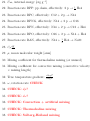
1. cd into the directory stars/. This is the directory that contains the code subdirectory.
2. If you’re running on a computer cluster, you probably want
to link the executable statically. To do this, edit the file
CMakeLists.txt and set the option WANT STATIC to on.
3. Configure and compile (starting from the directory stars/).
Use CMake (type cmake --version to see whether CMake is
installed):
(a) mkdir build && cd build
(b) cmake ..
(c) make
(d) cd -
If you updated the code (and build/ already exists) and compilation doesn’t work, you should type make clean before
step 3b. If the code still doesn’t compile, do rm -rf build/
before step 3a. Note that at step 3b, CMake chooses a compiler. To overrule this, execute e.g. FC=gfortran cmake ..
instead. Step 3c may produce some remarks and should produce the binary executable code/ev.
4. It is very useful to set the environment variable to the path
of the stars/ directory, e.g.
export evpath="/home/user/codes/stars/".12 This line
should probably go into your ∼/.bashrc. Check with echo
$evpath.
5. It is very useful to put ev in your path. You could do one of
these:
(a) PATH=${PATH}:`echo ${evpath}/code` (to add the directory where ev sits to your path. Again, you should
add this to your ∼/.bashrc).
(b) cp code/ev ∼/bin/ (if ∼/bin/ is in your path)
1.3
Running the code
Change this to using stars standard/ instead.
1. I assume you’re still in the stars/ directory.
1
I’m assuming you’re using bash. If you’re using csh, replace export a="b"
with setenv a "b" and ∼/.bashrc with ∼/.cshrc
2
Some compilers, e.g. gfortran don’t accept ∼/ but need e.g. /home/user/.
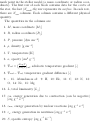
2. cd run; ls — This contains number of subdirectories with
different example runs. Let’s try the second one and copy the
contents in order to keep the original:
3. cp -r 02-single/ test-02 && cd test-02/ && ls — The
directory contains an example init.dat and two example
init.run files. You need one of each to start a run. Let’s use
init.run m4, which evolves a 4 M star:
4. cp init.run m4 init.run
5. We’re all ready to start the code. The default syntax is:
<path>/ev <output-file base name> <metallicity> <st
directory>
and could be e.g.:
∼/codes/stars/code/ev star 02 ∼/codes/stars/
which is a little annoying, since your code directory is probably not going to move around your hard disc a lot. Hence
step 5 in section 1.2, which allows us to remove the path from
the ev command and step 4 with which we can leave out the
last command-line option altogether. Using those steps thus
reduces things to:
ev star 02
The remaining options mean that all my output files will be
called star.* and that I want to use solar metallicity (02
means Z = 0.02, Z = 0.001 would reduce to 001, etc. In fact,
Z = 0.02 is the default option, so I could leave it out and run
my first model as:
ev star
1.4
Stopping the code
To terminate a running model properly, you type echo 1 > fort.11
in the directory where the code is running. (Presumably, we’ll want
to replace fort.11 with a proper file name at some point, to facilitate running and terminating different versions of the code in the
same directory independently).
2
Modus operandi
The stellar evolution code ev is designed to be a binary-evolution
code. However, it can be used to compute the evolution of both
single and binary stars, and for binaries, there are several possible
modes to use the code in. These modes are set by two parameters
in init.run: ISB (1 or 2, depending on whether we want to evolve
one or two stars) and KTW (1 or 2 for non-simultaneous or nonsimultaneous binary mode, respectively).
2.1
Single stars
Since ev is a binary-evolution code, single stars are in effect in a
binary. Since you don’t want to waste your undoubtedly valuable
(CPU) time on computing the secondary, we set ISB=1 (single star)
and KTW=1 (non-TWIN mode — I’m not sure whether it matters,
but it seems a safe way to go).
However, here we only tell the code not to compute a model of
the secondary. It will still exist, as a point mass. The important
thing is that Roche lobes will still be defined, and it is important
to set the initial orbital period (PER, in init.run) to a sufficiently
high value to make sure your ‘single star’ will not fill its Roche
lobe. In addition, I usually set BMS to twice SM, to make sure you
don’t end up with a negative secondary mass. Experienced users
may want to switch off the equations that govern orbital evolution,
mass transfer, etc., in init.dat, see Sect. 4.6.
2.2
Binary stars
When computing the evolution of a binary, we can choose whether
we want to compute a full model of the secondary, or regard it
as a point mass (which can be useful when dealing with WD, NS
or BH accretors). If we want to compute a detailed model of the
secondary, we can choose between non-simultaneous evolution, in
which the primary is evolved for KP timesteps, before switching to
the secondary to catch up in age with the primary, and simultaneous
evolution (also known as TWIN mode), in which both components
are evolved at the same time, and mass transfer is taken into account implicitly (this is necessary if e.g. both stars have winds).
2.2.1
Primary + compact companion (point mass)
Evolving a binary with a point mass is essentially similar to singlestar mode, except that we will set the binary mass (BMS) and the
orbital period (PER) to the values we want, and we make sure
that exactly one of CMT or CMS is non-zero when using a version of init.dat for single-star evolution. You may want to check
whether the equations for orbital evolution and mass transfer are
being solved, see Sect. 4.6, but in principle this is not necessary. We
also set ISB=1 (evolve one star) and KTW=1 (non-simultaneous
mode) in init.dat.
2.2.2
Two components, non-simultaneous
This mode was the original way of computing the evolution of a
binary: the primary is evolved for KP timesteps, after which the
code switches to the secondary, evolves it to the same age as the
primary, and it keeps alternating between the two.
This approximates binary evolution sufficiently well for many
cases, but it will not when the secondary has a non-negligible wind,
or when the secondary fills it’s Roche lobe. In other words, all
changes to the orbit are made by the primary and the secondary
cannot have any influence on the orbit (since if it would, this would
affect the evolution of a Roche-lobe-filling primary, which has already been established in the previous semi-cycle).
During the first semi-cycle, while evolving the primary, data
on orbital evolution and mass transfer are stored in file.io12,
which are then read again during the second semi-cycle, where the
secondary is evolved.
In order to use this mode, set ISB=2 (evolve two stars) and
KTW=1 (non-simultaneous mode), and make sure you solve equations for mass transfer and orbital evolution (see Sect. 4.6).
2.2.3
Two components, simultaneous (TWIN mode)
TWIN mode was developed by Peter Eggleton as an improvement
of the non-simultaneous evolution in the previous section. It allows
mass loss and mass transfer from the secondary, and, in particular, contact binaries (at least in principle). Both stars are evolved
simultaneously, and mass transfer is solved implicitly.
In order to use TWIN mode, set ISB=2 (evolve two stars) and
KTW=2 (simultaneous mode), and make sure you solve all necessary equations (see Sect. 4.6).
2.3
Creating grids in mass, mass ratio and period
This is currently broken, due to the way (output?) files
are opened.
Apart from computing the model of a single binary (or one single
star), the code can be used to compute grids of models, for ranges
of initial primary mass, mass ratio and orbital period.
When you want to compute a grid, the initial binary parameters
SM, BMS and PER in init.run must be set to negative values, to
ensure that they don’t override the grid values.
If you want to compute only one model, make sure KML = KQL
= KXL = 1.
See Section 5.2 for more details.
3
3.1
IO files
Input files
init.dat Initialisation file. Contains the details of the numerics,
equations to solve and physics to include while running a stellar model (unit 22).
init.run Run control file. Controls the start and stop conditions
1
for different models in a run. One can loop over M1 , q ≡ M
M2
and Pi . Output from different loops is stored in files with
different names or in different directories. The file file.list
gives an overview of which model is stored where (unit 23).
3.2
Output files
As an example I chose the file name file.* for the model files.
file.out1,2 Main output file, showing what the stars are doing at
that moment. These files are useful as ‘screen output’ (units
1,2).
file.out Pruned version of the above two files (unit 9). To be
removed?
file.io12 Contains orbital and mass-transfer data from star 1, to
be used in star 2 in non-TWIN binary mode (unit 3).
file.mod Contains a number of complete stellar-structure output
blocks. A block from this file can serve as input for a next
model (unit 15).
file.last1,2 Contains complete structure of last and pre-last mod
when lucky, that can serve as input for a next run (units
13,14).
file.list Shows the starting time and path of a run and tables
the properties of the different models and the file names or
directories in which they are stored (unit 50).
file.log Shows how the code was terminated, if terminated properly (unit 8).
file.mas Creation of helper file to find the proper ZAMS model
from zams.mod (unit 29?)
file.plt1,2 Contains stellar-evolution data, one model per line
(units 31,32).
file.mdl1,2 Contains a number of complete stellar-structure models, one mesh point per line (units 33,34).
file.nucout1,2 Main abundances “screen-output file” true? (uni
35,36).
file.nucplt1,2 Contains abundances in stellar-evolution models,
one model per line true? (units 37,38).
file.nucmdl1,2 Contains abundances in stellar-structure models,
one mesh point per line true? (units 39,40).
3.3
Data files
The files below can be found in the input/ directory of the installation and are used for data input (ZAMS, opacities, etc.):
zahb*.mod Input structure model for post-helium-flash models (unit
12)
zahb.dat “init.dat” for post-helium-flash models (unit 24?)
zams.mod Input structure model for ZAMS models (unit 16)
zams.mas Reading of helper file to find the proper ZAMS model
from zams.mod (unit 19?)
phys.z* opacity tables for certain metallicity (unit 20?)
lt2ubv.dat Data to compute magnitudes and colours from L, Teff
(unit 21?)
nucdata.dat Data to compute nuclear reactions (unit 26?)
mutate.dat Data to do something with merger products?
(unit 63)
COtables z* Data to compute opacities (unit 41)
physinfo.dat To do (unit 42)
rates.dat To do (unit 43)
nrates.dat To do (unit 44)
3.4
Temporary files
fort.11 is used to create stop the code, using the command echo
1 > fort.11
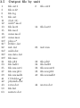
3.5
1
3
8
9
11
12
13
15
16
19?
20?
21?
22
24?
26?
29?
31
33
35
37
39
41
42
43
50
63
Output file by unit
file.out1
file.io12
file.log
file.out
(fort.11)
zahb*.mod
file.last1
file.mod
zams.mod
zams.mas
phys.z*
lt2ubv.dat
init.dat
zahb.dat
nucdata.dat
file.mas
file.plt1
file.mdl1
file.nucout1
file.nucplt1
file.nucmdl1
COtables z*
physinfo.dat
rates.dat
file.list
mutate.dat
2
file.out2
14
file.last2
23
init.run
32
34
36
38
40
file.plt2
file.mdl2
file.nucout2
file.nucplt2
file.nucmdl2
44
nrates.dat
4
init.dat
The init.dat file contains the parameters that are needed to control the numerical details of the code, the differential equations
that need to be solved using which variables and boundary conditions and which physics (nucleosynthesis, rotation, stellar wind,
overshooting, et cetera). The new format (post–2005 CVS version)
contains one parameter (either scalar or array) per line. If a variable name is used multiple times (on multiple lines), the last entry
will be used. This is useful for experimenting with values, while
keeping the old ones in the file. If a variable is not mentioned at
all, the (hard-coded) default value is used.
Thus, the order of the parameters does not matter, but for reasons of clarity and consistency it is a good practice to keep the
order used here.
4.1
Output
KT(1) – (4) also known as KT1, KT2, KT3, KT4:
KT1 Print internal details of every KT1-th model to file.out1,2
and file.mdl1,2 (20 or 200)
KT2 Print internal details at every KT2-th mesh point of the KT1th model (file.out1,2 only) (1 or 2)
KT3 Print KT3 ‘pages’ of details for every KT1-th model to file.ou
(1, 2 or 3)
KT4 Print a five-line summary of every KT4-th model to file.out1
and save every KT4-th evolution model to file.plt1,2 (1, 2
or 4)
KT5 Print a one-line summary of each iteration of each model
to file.out1,2, except for the first KT5 iterations of each
model (0 or 2)
KSV an output model is stored in file.mod (fort.15) after every KSV-th timestep in a run, in the form needed as input for
a further run. The last model of a run is automatically also
stored, in file.last* (fort.13,14). (5000)
KSX(45) The first 15 integers identify the quantities, such as
log ρ, L, X(4 He), . . . , which are to be printed in columns on
the first ‘page’ of structure details for every KT1-th model.
The next two lots of 15 relate to the optional further ‘pages’.
See section 13.
4.2
Mesh spacing
KH2 The number of mesh points you want; if this differs from KH
the code should interpolate in the given model to produce a
new one; but you must also set JCH to ≥ 2 to implement this
change (199)
JCH If JCH > 1, the REMESH initialises the model in various
ways:
JCH = 1 Does nothing.
JCH = 2 Initialises some new variables, for instance the
mass,
JCH = 3 = (2) + constructs new mesh spacing by interpolation,
JCH = 4 = (3) + initialises composition to uniformity (for
At least in some cases JMX in init.run must be 0 if JCH > 1
in order for the first model to converge.
CT(1) – (10) coefficients used in the mesh-spacing function Q:
Q = CT(4)*log(P) + CT(5)*log(P+CT(9)) +
CT(7)*log(T) - CT(7)*log(T + CT(10)) CT(3)*log(1 + R2 / CT(8)) +
log( CT(6) * Mc2/3 / (CT(6)*Mc2/3 + M2/3 ) )
CT(1) Unused (0.00)
CT(2) Used for Luminosity weight (0.00, reasonable values
seem to be 0.01-1.0, and perhaps other values)
CT(3) Used for Radius weight, together with CT(8) (0.05)
CT(4) Used for Pressure weight, together with CT(5,10)
(0.05)
CT(5) Used for Pressure weight, together with CT(4,10)
(0.15)
CT(6) Used for Mass weight (0.02)
CT(7) Used for Temperature weight, together with CT(10)
(0.45)
CT(8) Used for Radius weight, together with CT(3) (1.E-4)
CT(9) Used for Pressure weight, together with CT(4,5) (1.E1
CT(10) Used for Temperature weight, together with CT(7)
(2.E4)
use smooth remesher Switch for the new “smooth” remesher.
See also start with rigid rotation in init.run (.false.)
relax loaded model Switch for the new “smooth” remesher. (.tr
4.3
Time steps
KN The number of variables that will be used for determining the
next time step.
KJN(1)-KJN(40) The first KN of these identify the variables to
be used for determining the next time step, see section 14.
CT1 The next timestep cannot (normally) be less than CT1 times
present timestep (0.8, 0.9 or 1.0)
CT2 The next timestep cannot be greater than CT2 times present
timestep. If both CT1 and CT2 are 1.0, then the timestep is
constant, of course (which is useful for constructing a ZAMS
by artificial ‘mass-gain’) – except that if a model fails to converge the timestep will be multiplied by CT3 (1.1, 1.05 or
1.0)
CT3 when the solution package fails to converge, the code retreats
to the second-last converged model, and continues with the
timestep decreased by the factor CT3. (0.3 or 0.5)
4.4
Convergence
KR1 The maximum number of iterations allowed on the first timest
(20)
KR2 The maximum number of iterations allowed on later timesteps
(12) If you want to see output when the code is struggeling
to converge a model, make sure KR2 > KT5.
climit Limit changes in variables during iterations (1.0d-1)
use quadratic predictions Normally, the code uses linear extrapolation to predict values for the first iteration on the next
timestep. Set this switch to .true. to use quadratic extrapolation, which can be slightly more accurate. (.false.)
use fudge control (obsolete, present for backward compatibility) Used to switch certain “fudges” on and off, as needed.
Now unused. (.true.)
allow extension (unused, present for backward compatibility)
Allow the code to do a few extra iterations if it is close to
converging when it runs out of iterations. A better approach
is to set a convergence window. (.false.)
allow underrelaxation Allow the code to suppress the diffusion
terms in the composition equations and then switch them on
slowly as the code iterates. (.false.)
allow overrelaxation Allow the code to magnify the diffusion
terms in the composition equations and then relax them to
their normal value as the code iterates. (.false.)
allow egenrelaxation Allow the code to fall back to the energy
generation rate from the previous timestep and then smoothly
transition to its current value as the code iterates. (.false.)
allow mdotrelaxation Allow the code to suppress mass loss from
stellar winds or RLOF and switch it on smoothly as the code
iterates. (.false.)
allow avmurelaxation Together with use previous mu determine
whether the current or the previous value of the mean molecular weight should be used to estimate the effect of thermohaline mixing. Normally best left alone. (.false.)
use previous mu Use the previous value of the molecular weight
rather than the current value when calculating the effect of
thermohaline mixing (for numerical stability reasons). (.true.
off centre weight Used to scale the weighting of terms in the difference equations. A large value means that the weighting
is always central, a smaller value means that the weighting
moves off-centre for mesh points where the timestep becomes
of the order of the thermal conduction time. See Sugimoto
(1970) for details. (1.0d16)
4.5
Accuracy
EP(1) – (3) also known as EPS, DEL, DH0. They determine how
the code behaves when the mean modulus change in DH in the
latest iteration equals ERR (see Writeup, section 1.6):
EPS The accuracy to which SOLVER is required to solve the equations; if ERR < EPS, the model has converged. (10−6 )
wanted eps The desired accuracy. The solver will aim for an accuracy of wanted eps < ERR < EPS. This has no effect if
wanted eps ≤ EPS. (1.0d-8)
DEL If ERR > EPS, the corrections applied to DH are reduced by
the factor DEL/ERR. (10−2 )
DH0 Variation in H to compute numerical derivatives.
(10−7 )
CDC(1) – (5): CDD is the mean increment, r.m.s.-wise, that you
would like in one timestep. Different evolutionary phases have
different CDD’s (identified here by name rather than by number):
cdc ms: CDD = cdc ms, between ZAMS and core hydrogen
0.04 (corresponding to the beginning of the hook in stars
above ∼ 1.2M ). (0.04 or 0.01)
cdc ems: CDD = cdc ms * cdc ems, between the beginning
of the hook and hydrogen exhaustion. The purpose is to
reduce the timestep so that the hook is properly resolved.
(0.15 or 1.0)
cdc hg: CDD = cdc ms * cdc hg, between core hydrogen exhaustion and the base of the giant branch. The intention
is to increase the timestep during the Hertzsprung gap.
(3.0 or 1.0)
cdc 1dup: CDD = cdc ms*cdc 1dup, during first dredgeup
(1DUP) on the giant branch. (0.10 or 1.0)
cdc hec: CDD = cdc ms*cdc hec, for evolution during core
He burning. (0.0625 or 0.25)
cdc hes: CDD = cdc ms*cdc hes, for further evolution until
the He shell nearly catches up with the H shell. (0.25 or
1.0)
cdc dblsh: CDD = cdc ms*cdc dblsh, for double-shell-burnin
The intention is to either make the timestep large and
skip over the thermal pulsing phase (if ≥ 1), or to cut
back the timestep and resolve the thermal pulses (if < 1).
(1.0 or 4.0)
cdc rlof: CDD = CDD*cdc rlof, to reduce the timestep if the
system is moving closer to Roche lobe overflow (RLOF).
The criterion is that the star is close to filling its Roche
lobe and expanding. (0.05 or 1.0)
cdc rlof reduce: CDD = CDD*cdc rlof reduce, to keep the
timestep smaller while the system detaches after RLOF.
The criterion is that the star is close to filling its Roche
lobe and shrinking. (0.25 or 1.0)
4.6
Equations, variables and boundary conditions
See also Writeup, section 1.5
KE1, KE2 The number of first and second order difference equations respectively
KE3 Subset of KE1 that involves 3 rather than 2 adjacent mesh
points (not yet used, keep 0)
KBC The number of boundary conditions
KEV The number of eigenvalues
KFN The number of ‘intermediate functions’
JH1 – JH3 Used for debugging purposes
See also Writeup, section 1.5
kp var Determines which and in which order the independent variables are used (max 40 integers); a.k.a. id(11:50), ig(11:50)
in e.g. solver().
kp eqn Determines which and in which order the difference equations are used (max 40 integers); a.k.a. id(51:90), ig(51:90)
in e.g. solver().
kp bc Determines which in which order the boundary conditions
are used (max 40 integers); a.k.a. id(91:130), ig(91:130)
in e.g. solver().
The same contents as lines 5-11, not currently used. See the
end of section 1.5 of Writeup.
4.7
Equation of state
KCL(1) – (7) also known as KCL, KION, KAM, KOP, KCC,
KNUC, KCN:
KCL Unity includes the Coulomb correction to pressure etc; zero
suppresses it. (1)
KION EoS does the ionisation of the first KION elements in the
list H, He, C, N, O, Ne, Mg, Si, Fe. No other elements are
included. KION = 5 is about optimal. Do not try 9. (5)
KOP If unity, code should use spline interpolation in tables of
opacity; if zero, simple bi-linear interpolation (1)
KCN If 0, gives standard nuclear network. If 1, gives a CNOequilibrium fudge for ZAMS models: see FUNCS1 (0)
eos include pairproduction Should the equation-of-state include
the effects of pair production? This is only important in the
very late burning stages of very massive stars. Positrons are
only calculated if their degeneracy parameter ≥ -15.0 — otherwise they are negligible anyway. (.false.)
4.8
Nucleosynthesis
CH value for initialising X(1 H) as a fraction of the total composition; only used for ZAMS models, with JCH = 4. The default
value, CH = −1, tells the code to use the value provided with
the ZAMS model. For some (lower?) metallicities and some
initial masses (M ∼ 0.8 M ?) the ZAMS model may not
converge. In such a case setting ML1 to the nearest value for
which the ZAMS model converges, and SM to the desired mass
(in init.run) may help out. (-1.0)
CC, CN, CO, CNE, CMG, CSI, CFE values for initialising X
... X(56 Fe), as fractions of the total metallicity Z (= CZS
in input/phys.z* (fort.20)); only used for ZAMS models,
with JCH = 4.
(0.176, 0.052, 0.502, 0.092, 0.034, 0.072,
0.072)
kr nucsyn Number of allowed iterations for the nucleosynthesis
code (60)
4.9
Rotation
See also start with rigid rotation in init.run.
rigid rotation Use rigid rotation, or differential rotation? (.true.)
4.10
Stellar structure
KTH(1) – (4), alias KTH – KZ:
KTH th = KTH ∗ (T DS/Dt); so you can ignore T DS/Dt if you
want (1 or 0)
KX DX(1 H)/Dt = KX ∗ (burning rate of 1 H); so you can ignore
the composition change while keeping the energy production
(1 or 0)
KY The same, for 4 He (1 or 0)
KZ The same, for
12
C and
16
O (1 or 0)
CALP The mixing-length ratio (2.0)
CU Along with COS and CPS, a ‘convective overshooting’ parameter, see CRD. (0.1)
COS A convective overshooting parameter for H-burning cores, see
CRD. Zero implies no overshooting. (0.12)
CPS as COS, but for He-burning cores.
(0.12)
CRD The diffusion coefficient σ for convective mixing is taken to
be CRD times the ‘legitimate’ rate from mixing-length theory; except that an approximate multiple of [∇r − ∇a ]1/3 is
replaced by the same multiple of [∇r − ∇a + ∇OS ]2 , where
∇OS ≡
(2.5 + 20β∗ +
16β∗2 )
COS
, β∗
(CU · ∂ log m/∂ log P + 1)
The usual CRD is 10−2 or 10−4 .
CXB Defines the boundary of a core to be at X(1 H) or X(4 He) =
CXB; for printout and envelope binding energy (0.15)
CGR Defines the boundary between a convection zone and a semiconvection zone, for printout purposes only, to be at ∇r −∇a +
∇OS = CGR (0.001)
CEA A constant energy rate ENC can be added to nuc + th − ν .
An increasing ENC can push a star back from the ZAMS
to the Hayashi track. CEA and CET determine how ENC
changes with time (1.0E2)
CET The equation for the growth of ENC with time is d ENC/dt
= ENC×CET×(1 – ENC/CEA), so that ENC increases exponentially on the assigned timescale 1/CET (yr), until saturating at ENC ∼ CEA. (1.0E-6)
4.11
Mass loss
Individual mass loss recipe switches. These also turn on recipes
when smart mass loss is used, although that does store its own set
of mass loss options (to keep it more modular).
At the surface,
Ṁ = − CMT·ξ − CMS·[log(r/rlobe )]3 + CMI·m − CMR·1.3×10−
− CMJ · ṀJNH − CML · ζ(L, r, m, Prot )
([X] ≡ X if X > 0 and 0 if X < 0). The equation above is no longer
complete, as new wind mass-loss prescriptions have been added, as
described in the next subsection. See Sect. 4.11.1 for a detailed
description of the parameters CMR, CMJ and CML, which deal
with wind mass loss, and Sect. 4.11.2 for the parameters CMT and
CMS, which describe the mass transfer.
CMI a constant mass-gain/loss rate, for running up or down the
ZAMS, (yr−1 ) (0.0, ± 5.0D-9 or ±1.0D-6)
cmi mode Changes the interpretation of CMI. If cmi mode =
1, then CMI represents a time scale for exponential massgain/loss (Ṁ = M · CMI). If cmi mode = 2, then CMI represents a mass-gain/loss rate in solar masses per year. (1)
4.11.1
Wind mass loss
smart mass loss Turn on the smart-mass-loss routine, which picks
an appropriate recipe depending on the stellar parameters.
This is an alternative for the De Jager rate and replaces it
when smart mass loss is switched on. (0.0 (off))
CMR Multiplier
mass-loss rate: Ṁ = CMR ×
for a−5Reimers-like
1.3×10 L 10
M × max
,
(0.0 or 0.2–1.0)
CMJ Multiplier for the De Jager mass-loss rate for luminous stars
(de Jager et al 1988) (0.0 or 1.0)
zscaling mdot Scaling with metallicity applied to De Jager massloss rate in funcs1 (0.8)
CMV Multiplier for the Vink mass-loss rate
CMK Multiplier for the Kudritzki 2002 mass-loss rate
CMNL Multiplier for the Nugis & Lamers mass-loss rate (for
Wolf-Rayet stars)
CMRR Multiplier for the real Reimers mass-loss rate
CMVW Multiplier for the Vasiliadis & Wood (1993ApJ...413..641V
mass-loss rate (superwind for late AGB stars)
CMSC Multiplier for the Schröder & Cuntz mass-loss rate
CMW Multiplier for the Wachter et al. (2002A&A...384..452W)
mass-loss rate (superwind for late AGB stars)
CMAL Multiplier for Achmad & Lamers the mass-loss rate (for
A supergiants)
cphotontire Switch to include photon tiring (0.0)
CML A mass-loss rate as obtained from a simplistic dynamo theory (0.0 or 1.0)
CHL A factor multiplying the rate of ang. mom. loss associated
with the rate of mass loss ζ, according to the same dynamo
model. (0.0 or 1.0)
cmdotrot hlw (Multiplier for?) rotationally enhanced mass loss
rate by Heger, Langer & Woosely Set at most one of these!
cmdotrot mm (Multiplier for?) rotationally enhanced mass loss
rate by Maeder & Meynet. Set at most one of these!
CTF A factor multiplying an expression for the rate of tidal friction. (0.0 or 0.01)
CLT A coefficient used in the estimation of heat flux between components in contact. It does not really work yet (or does it?).
4.11.2
Mass transfer
CMT one of two versions of MT by RLOF. CMS & CMT are
alternatives; set one of them to zero (0.0, or 1.0D-2–1.0D2
for stars of increasing mass (?)) For contact binaries, CMT
is preferred (or even mandatory).
CMS one of two versions of MT by RLOF. CMS & CMT are
alternatives; set one to zero (0.0, or 1.0D0 – 1.0D4). A
too-high value can crash the model at the onset of MT. Use
CMT for contact binaries.
cmtel Eddington-limited accretion factor (depends on the stellar
parameters) (0.0d0 or 1.0d0)
cmtwl Angular-momentum limited accretion factor (depends on
the stellar parameters) (0.0d0 or 1.0d0)
ccac Switch for composition accretion (0.0d0)
cgrs Switch for gravitational settling (0.0d0)
CPA ‘partial accretion’: the fraction of one star’s wind that is
accreted by the other. (0.0)
CBR ‘bipolar re-emission’: the fraction of material accreted by a
star that is ejected in bipolar jets. Needed for CVs, LMXBs.
(0.0)
CSU ‘spin-up’, specifically of the gainer due to accretion. CSU
is the specific angular momentum (AM) relative to orbital
(OAM), taken out of the orbit by material leaving the L1
point, acquiring AM due to Coriolis force, and landing on the
other star - so OAM is converted to gainer’s internal AM.
Does not seem to work properly... yet. (0.0)
CSD ‘spin-down’; the same process also spins down the loser, I
suppose, though not by as much. Does not seem to work
properly... yet. (0.0)
CDF this is used to convert a step-function into a ‘smoothed’ step
function: see Writeup p.27. (0.01)
CGW A switch to turn gravitational radiation on and off (0.0 or
1.0)
CSO A switch to turn spin-orbit coupling on and off (0.0 or 1.0)
CMB A multiplication factor to determine the strength of an alternative magnetic braking law, currently the one by Rappaport,
Verbunt & Joss, 1983. (0.0 – 1.0)
4.12
Mixing
artmix Artificial mixing coefficient [cm2 /s]. Set it to 1.0 to mix
csmc Semi-convection efficiency, after Langer (1991) (4.0d-2)
cdsi Switch for the dynamical shear instability (1.0d0)
cshi Switch for the solberg-hoiland instability (not implemented)
(1.0d0)
cssi Switch for the secular shear instability (1.0d0)
cesc Switch for the Eddington-sweet circulation (1.0d0)
cgsf Switch for the goldreich-schubert-fricke instability (1.0d0)
cfmu Weight of mu gradient in rotational instabilities [see Heger’s
thesis page 36 and Pinsonneault] (5.0d-2)
cfc Ratio of turbulent viscosity over the diffusion coefficient [see
Heger’s thesis page 35] (3.3d-2)
convection scheme To do (1)
4.13
Cetera
enc parachute Emergency energy-generation term, normally set
to 0. This cannot be set from the input file. It will be set by
remesh if there is no nuclear energy generation in the initial
model at all. In that case, the first iteration(s) will return
LOM = 0.0 throughout the star because the thermal-energy
term is initially 0 as well. this is a numerical fudge to remove the resulting singularity. This term will be set to L/M
(constant energy generation throughout the star) and will be
reduced to 0 by printb. (0.0)
5
init.run
The init.run file contains parameters that control how to start
and stop the run. You have to decide on each of four options, each
giving two alternatives. The options are
a) single stars or binary stars
b) new, i.e. starting from scratch (ZAMS), or old, e.g. starting
from the end of a previous run.
c) independent evolution (‘normal mode’), or simultaneous evolution (‘TWIN mode’), of the components.
d) a ‘one-model’ or ‘grid’ run. A grid means several runs, one
after the other (but simultaneous using the massively parallel version, not described here), with the three parameters
of primary mass, mass ratio and orbital period being cycled
through. One-shot means what it says.
Not all 16 possibilities make sense: e.g. if you are doing TWIN
evolution, you won’t want single stars. Many but not all of the
remaining possibilities should be viable.
5.1
Mode of operation
ISB, KTW, IP1, IM1, IP2, IM2, KPT, KP
ISB evolve one or two stars. ISB = 1 implies only one star should
be computed in detail; ISB = 2 evolves both components of
a binary. For single stars, you may still use the outer (first)
cycle for masses. The inner 2 cycles are automatically set
to do only one case each. The mass ratio and the period
be supplied. The period should be so large that there is no
danger of RLOF (see also Sect. 2). (e.g. XL = 7.0, meaning
a period of ∼ 107 d).
KTW 1 for normal, non-simultaneous operation; 2 for TWIN mode
where both stars are solved simultaneously. See Sect. 2 for
more detail.
IP1 the number (13 – 16) of the file (fort.13 – fort.16) where the
initial model for ∗1 is to be taken from. ZAMS models are on
fort.16.
IM1 the sequential number of the model required on fort.IP1. This
is computed automatically, from later data, if the ZAMS file
fort.16 is used, so that if IP1 is 16, it doesn’t matter what
value you give for IM1, but you have to give a value.
IP2 as IP1, but for ∗2.
IM2 as IM1, but for ∗2.
KPT the maximum number of timesteps for each component (2000
to 4000 for fairly complete evolution). You may set KPT
equal to -1 to indicate that the code should run until one
of the termination conditions is met, in other words, the
code will not stop when it reaches a predetermined number
of timesteps.
KP Do approximately KP of ∗1, then enough of ∗2 to catch up
with ∗1, then another ∼ KP of ∗1, etc, so that if ∗2 breaks
down before ∗1 you don’t waste a lot of calculation on ∗1.
You will seldom get exactly the number of timesteps that you
ask for. For single stars, KP is set to KPT automatically.
5.2
Grids of masses and periods
ML1, DML, KML; QL1, DQL, KQL; XL1, DXL, KXL
These three lines contain parameters for 3 nested loops (mass, mass
ratio, and initial period) to be run through. Each loop has: starting
value; increment; number of cases (1 more than the number of
increments).
• The first (outer) loop is: log10 (mass, solar units), starting
at ML1, increasing by steps of DML to ML1 + (KML – 1) .
DML
• The second loop is: log10 (mass ratio in sense {larger/smaller})
starting at QL1, increasing by steps of DQL to QL1 + (KQL
– 1) . DQL
• The third (inner) loop is: X ≡ log10 (orbital period /period
necessary for ∗1 to fill its Roche lobe when still on the ZAMS),
starting at XL1, increasing by steps of DXL to XL1 + (KXL
– 1) . DXL.
• If you want to compute only one model (single or binary), set
KML = KQL = KXL = 1.
When a grid is computed, the initial binary parameters SM, BMS
and PER must be set to negative values, to ensure that they don’t
override the grid values.
5.3
Rotation and eccentricity
ROT, KR, EX
ROT, KR KR = 1: Prot for each star = rotational breakup period
ROT
KR = 2: Prot for each star = max(1.05 * rotational breakup
period, orbital period * 10ROT ) PERC: breakup or
RLOF at ZAMS?
KR ≥ 3: set Prot = Porb ; (almost) synchronous rotation
EX the initial eccentricity.
5.4
Initial binary parameters
SM, DTY, AGE, PER, BMS, ECC, P, ENC, JMX
(a.k.a. AX(1-8), JMX). The AX’s are optional replacements for
the values of SM, . . . , ENC that the code would normally pick up
in fort.IP1 from some previous run, or from the ZAMS library
(fort.16). JMX similarly is an optional replacement for JMOD.
They are only applied if they are non-negative. Thus you can replace only one, or several.
SM Primary mass [M ]
DTY Time step [yr]
AGE Model age [yr]
PER Orbital period [d – or fraction of break-up?]
BMS Total binary mass [M ]
ECC Orbital eccentricity
P Spin period of the primary [d]
ENC Artificial energy rate, see CEA and CET [?]
JMX New model number (JMOD). Set to −1 to keep unchanged,
to 0 to set the mass of a ZAMS model using the loop parameters ML1,QL1 above, ignoring SM (when using IP1,2=16)
True? and to any positive value to start counting models at
that value. For grids looping over primary mass and mass ratio, you must set JMX to 0! In some cases, when restarting
an evolved model, you seem to have to set JMX to > 0!
START WITH RIGID ROTATION
Can be TRUE or FALSE.
5.5
Termination conditions
UC:
The last three lines are a set of 21 criteria (UC(1–21)) to determine
when the run is to be ended (e.g. when the age is greater than
2 × 1010 yr), or when some special procedure should be initiated
(e.g. the He-flash evasion). You’ll have to read the end of printb.f
to figure them out completely. In many cases the code is stopped
by changing the termination code JO.
UC(1-7):
UC(1): (rlf1) Terminate if FLR(=RLF?) (Sect. 9, nr 29) of star 1
exceeds this number (JO = 4) (0.1)
UC(2): (age) Terminate if the age of the model in years exceeds
this number (JO = 5) (2e10)
UC(3): (LCarb) Terminate if LC > this number (JO = 6) (100)
UC(4): (rlf2) Terminate if FLR(=RLF?) (Sect. 9, nr 29) of star 2
exceeds this number (JO = 7) (0.2)
UC(5): (LHe) Initiate He-flash evasion if LHe > this number, together with UC(6) (JO = 8) (1e3, lower for M∗ ≈ 2M )
UC(6): (rho) Initiate He-flash evasion if log ρc > this value (?),
together with UC(5) (JO = 8) (5.3)
UC(7): (MCO) Terminate if degenerate CO-core exceeds this mass
together with UC(8) (JO = 9) (1.2)
UC(8-14):
UC(8): (rho) Terminate if log ρc > this value (?), together with
UC(7) (JO = 9) (6.3)
UC(9): (mdot) Terminate if |Ṁ | > UC(9) ∗ M∗ /τKH (JO = 10)
(3e2)
UC(10): (XHe) Change eps (next number) if the core Helium
abundance drops below this number (0.15)
UC(11): (eps) If Ycore < XHe (previous number), set EPS to this
number. Do not use, keep this number 1e-6! (1e-6)
UC(12): (dtmin) Terminate if ∆ t < dtmin (in seconds?) (1e6)
UC(13): (sm8) The total mass the post-He-flash model should get,
can also be used manually! (1e3)
UC(14): (vmh8) The He-core mass he post-He-flash model should
get, can also be used manually! (1e3)
UC(15-21):
UC(15): (XH) If > 0: terminate if the core H-abundance drops
below this value, you can e.g. stop at the TAMS (JO = 51)
(0.0)
UC(16–21): Unused
6
file.mod
This file contains stellar structure output, that can be used as input.
The files file.last1,2 have the same format.
The file consists of one or more blocks, starting with a single line
with 13 model properties and followed by a block with one line per
mesh point with the independent variables. This block contains 24
columns of which only part is used. Some of them are ‘eigenvalues’
and have the same value for every mesh point.
6.1
Header
The first line of the file contains the 13 numbers:
1. M1 , the mass of the primary [M ]
2. ∆ t, time step [yr]
3. t, age of the model [yr]
4. Porb , the orbital period [day]
5. BM S, the total binary mass [M ]
6. e, the orbital eccentricity
7. Prot , the rotational period [day]
8. enc, artificial energy term [?]
9. kh, the number of mesh points and thus rows in the stellar
structure block below
10. kp, the total number of models to calculate
11. jmod, the current model number
12. jb, the number of this star in the binary [1 or 2]
13. jin, the number of independent variables and thus columns
in the stellar structure block below [24 for non-TWIN, 40 for
TWIN]
14. jf , do or do not overwrite overwrite I and φ (see below). Just
keep it 0. [0 or 2]
6.2
Blocks of stellar structure
Each block contains the contents of the variable H: 24 models for
non-TWIN models, and 40 for TWIN models. Columns 1–16 are reserved for the primary, 17–25 for binary parameters and 26–40 have
the same content as 1–16, but for the secondary in the TWIN case.
In the loop over all meshpoints in printb, the variable Q(1-24)
contains the same data as H(1-24,I) (or the corresponding variables for the secondary in a TWIN model) for each mesh point I.
Each line represents a mesh point, the first one usually the surface
of the star. The ‘eigenvalues’ are marked with (EV). The columns
are:
1. ln f , a dimensionless quantity closely related to electron degeneracy: for the case where electrons are non-degenerate and
non-relativistic, f ∼ 108 ρ/T 1.5
2. ln T , logarithmic temperature [K]
3. X16, mass abundance fraction of
16
O
4. m, mass [1033 g]
5. X1, mass abundance fraction of 1 H
6. C, the gradient of mesh-spacing function Q(f, T, m, r) with
respect to mesh point number K (EV).
7. ln r, logarithmic radius [1011 cm]
8. L, luminosity. Not logged, because it may be negative [1033 erg
9. X4, mass abundance fraction of 4 He
12
11. X20, mass abundance fraction of
20
Ne
12. I, the moment of inertia of the interior material [1055 g cm2 ]
13. Prot , the rotation period (days) of the star (EV).
14. φ - the centrifugal-gravitational potential [erg]
15. φs , the potential at the surface, minus the potential on the
L1 surface (EV) [erg]
16. X14, mass abundance fraction of
14
N
17. Horb , the orbital angular momentum (EV) [1050 gm cm2 s−1 ]
18. e, the orbital eccentricity (EV)
19. F , the flux of mass towards or away from the other star; a
function of depth and zero below L1 [1033 g s−1 ]
20. <empty>
21. <empty>
22. <empty>
23. <empty>
24. <empty>
25. – 40.: The same as variables 1–16, but for the secondary in
case of a TWIN model, otherwise empty (since jin (above)
equals 24 in that case).
7
file.log
This file contains the exit code with which the Eggleton code terminated. Usually, the file lists an explanation of these codes at the
top of the files, but for grids these lines may lack.
-2 Requested mesh too large (BEGINN)
-1 No timesteps required (STAR12)
0 Finished required timesteps (STAR12)
1 Failed; backup, reduce timestep (SOLVER)
2 Time step reduced below limit; quit (BACKUP)
3 Star 2 evolving beyond last star 1 model (NEXTDT)
4 Star 1: stellar radius exceeds Roche-lobe radius by limit (UC(1),
PRINTB)
5 Age greater than limit (UC(2), PRINTB)
6 Carbon burning exceeds limit (UC(3), PRINTB)
7 Star 2 radius exceeds Roche-lobe radius by limit (UC(4), PRINTB)
8 Close to helium flash (UC(5,6), PRINTB)
9 Massive (> 1.2M ), degenerate CO core (UC(7,8), PRINTB)
10 |Ṁ1 | exceeds limit (UC(9), PRINTB)
11 Impermissible FDT for star 2 (NEXTDT)
12 Time step reduced below limit – hydrogen left in the core; quit
14 Funny composition distribution (MH < MHe or MHe < MCO ,
PRINTB)
15 Terminated by hand (STAR12)
16 ZAHB model didn’t converge (MAIN)
17 Nucleosynthesis didn’t converge (BEGINN)
22 Time step reduced below limit – helium left in the core; quit
(BACKUP)
32 Time step reduced below limit – carbon left in the core; quit
(BACKUP)
51 End of MS (core hydrogen abundance below limit) (UC(15),
PRINTB)
52 Radius exceeds limit (PRINTB)
53 Convergence to target model reached minimum (PRINTB)
8
file.out{1,2}
Note: this section is about file.out1 and file.out2, not file.out
During a stellar evolution run short summaries of the stellar
parameters are written into the files file.out1 and file.out2. It
can be useful to watch this file while the code is running for example
by typing tail -f file.out1. This will show the last 10 lines of
the file.out1 file and refresh when file.out1 changes (exit with
Ctrl-C). The files start with a copy of init.dat. The rest of the
file consists of three different blocks of information:
Stellar snapshots: summaries of the star at a certain model number, e.g. its mass, age, central composition, etc.,
Stellar slices: detailed summaries of the interior of the star, e.g.
P ρ, T , etc., on every mesh point in the star,
Convergence info: information on the convergence of the set of
differential equations for each iteration.
How often these blocks of information are printed to the file can
be set with the parameters KT1 – KT5 in init.dat.
8.1
Stellar snapshots
Line 1:
M: Stellar mass [M ]
Porb: Orbital period [days]
xi: Mass transfer rate [M yr−1 ]
tn: Nuclear timescale
LH: Luminosity by Hydrogen burning
P(cr):
McHe: Mass of Helium core
CXH: Central H Abundance
CXHe: Central He abundance
CXC: Central C abundance
CXN: Central N abundance
CXO: Central O abundance
CXNe: Central Ne Abundance
CXMg: Central Mg abundance
Cpsi: Central value of the electron degeneracy parameter
Crho: Log Central density
CT: Log Central Temperature
Line 2:
dty: Time step [yr]
Prot: Rotational period [days]
zet: Mass loss rate other than Roche lobe overflow, e.g. wind. [M
yr−1 ]
tKh: Kelvin-Helmholtz timescale
LHe: Luminosity due to helium burning
RCZ:
McCO: Mass of CO core
TXH: H abundance at Tmax
TXHe: He abundance at Tmax
TXC: C abundance at Tmax
TXN: N abundance at Tmax
TXO: O abundance at Tmax
TXNe: Ne abundance at Tmax
TXMg: Mg abundance at Tmax
Tpsi: Value of the electron degeneracy parameter at Tmax
Trho: log Tmax
TT: log rho at Tmax
Line 3:
age: Stellar age [yr]
ecc: Orbital eccentricity
mdt: Mass loss [M yr−1 ]
tET: Envelope Turnover timescale of the convective envelope
LCO: Luminosity due to Carbon/Oxygen burning
DRCZ:
McNe: Mass of Neon Core
SXH: Surface abundance of H
SXHe: Surface abundance of He
SXC: Surface abundance of C
SXN: Surface abundance of N
SXO: Surface abundance of O
SXNe: Surface abundance of Ne
SXMg: Surface abundance of Mg
Spsi: Surface value of the electron-degeneracy parameter
Srho: Log Surface density
ST: Log Surface Temperature
Line 4:
cM: Companion Mass [M ]
RLF1: Relative Roche-lobe radius [log R/Rrlof ]
RLF2: Relative Roche-lobe radius [log R/Rrlof ]
DLT:
Lnu: Luminosity due to neutrino losses
RA/R: Alfvén radius [R ]
MH: Total hydrogen mass in the star [M ]
conv. bdries: Mass coordinates of convective boundaries (3 pairs)
logR: Log R
logL: log L
Line 5:
Horb: Orbital angular momentum
F1:
DF21:
BE:
Lth: Luminosity from contraction/expansion
Bp: Poloidal component of the magnetic field
MHe: Total helium mass in the star [M ]
semiconv. bdries: Mass coordinates of semiconvective boundaries
(3 pairs)
k**2: Dimensionless axis of gyration, if moment of inertia is calculated in the code.
8.2
Convergence info
Iter The first integer displays the number of iterations,
Err The logarithm of the total error,
Ferr The residue in the current iteration,
Fac The factor by which corrections are multiplied before being
applied. Normally 1.00, but may be smaller if the code has
trouble converging.
Then a list of numbers follows, in pairs of an integer and a float
(e.g. 79−9.2). There is one pair for each independent variable. The
integer indicates the mesh point in the star (1 indicates the surface)
where the largest error for this independent variable occurs and the
float indicates the log of the error in that mesh point. In practice
this means that (199 − 9.9) is a good thing since 10−9.9 is a very
small error, (98−3.1) is worrying and when the floats get to −2.0 or
larger something is really wrong. It is usually a good idea to scroll
up and look whether earlier blocks exist and, if so, to see whether
the same variables are causing the problems there — sometimes one
variable starts causing problems and then drags along others.
9
file.plt{1,2}
This file contains stellar evolutionary properties, for one structure
model per line. The first line contains the number of columns in
the output block. The block currently contains 81 columns, with
the following contents:
1. JMAD, Model number
2. t, Age [yr]
3. ∆t, time step [yr]
4. M , stellar mass [M ]
5. MHe , helium core mass [M ]
6. MCO , carbon-oxygen core mass [M ]
7. MONe , oxygen-neon core mass [M ]
8. log R, stellar radius [R ]
9. log L, stellar luminosity [L ]
10. log(Teff ), effective temperature [K]
11. log Tc , central temperature [K]
12. log Tmax , maximum temperature [K]
13. log ρc , central density [g cm−3 ]
14. log ρTmax , density at T = Tmax [g cm−3 ]
15. Ubind , binding energy of H envelope [erg/(1 M )]
3
16. LH , luminosity by hydrogen burning [L ]
17. LHe , luminosity by helium burning [L ]
18. LC , luminosity by carbon burning [L ]
19. Lν , neutrino luminosity [L ]
20. Lth , luminosity by release of thermal energy [L ]
21. Prot , rotational period [days]
22. VK2, K 2 ≡
I
,
M R2
with I the moment of inertia
23. Rcz , Depth (?) of convective envelope [R∗ ]
24. dRcz , Thickness (?) of convective envelope [R∗ ]
25. TET, Convective turnover timescale
26. RAF, Alfvén radius
27. BP, poloidal magnetic field
28. Porb , orbital period [days]
29. FLR = e log (R∗ /Rrl ), relative Roche Lobe Radius, also called
RLF
30. F1, ∼ Φsurf − ΦL1 [erg] ?
3
Multiply with 1.9891 × 1033 to get ergs. The reason for this confusing
solution is that values of 1040−50 erg don’t fit in a single-precision variable, and
that the value may be negative so that a log is no option.
31. Ṁ , total mass loss [M yr−1 ]
32. Ṁwind , wind mass loss [M yr−1 ]
33. Ṁmt , mass transfer rate [M yr−1 ]
34. Horb , orbital angular momentum [1050 g cm2 s−1 ]
35. dHorb /dt, total orbital angular momentum loss rate [1050 g
cm2 s−2 ]
36. dHgw /dt, change in Horb due to gravitational waves [1050 g
cm2 s−2 ]
37. dHwi /dt, change in Horb due to wind mass loss [1050 g cm2
s−2 ]
38. dHso /dt, change in Horb due to spin-orbit coupling [1050 g cm2
s−2 ]
39. dHml /dt, change in Hspin due to non-conservative mass transfer [1050 g cm2 s−2 ]
40. Mcomp , companion mass [M ]
41. e, orbital ellipticity
42. – 48. Surface abundances of: 42:H, 43:He, 44:C, 45:N, 46:O,
47:Ne, 48:Mg
49. – 55. Tmax abundances of: 49:H, 50:He, 51:C, 52:N, 53:O,
54:Ne, 55:Mg
56. – 62. Central abundances of: 56:H, 57:He, 58:C, 59:N, 60:O,
61:Ne, 62:Mg
63. – 68. Convection zone boundaries (mcb); > 0: beginning, < 0
end of zone (max. 3 sets)
69. – 74. Semi-convection zone boundaries (msb); > 0: beginning, < 0 end of zone (max. 3 sets)
75. – 80. Nuclear energy production zone (εnuc > εtresh ∼ 10L∗ /M
boundaries (mex); > 0: beginning, < 0 end of zone (max. 3
sets)
81. Qconv , the mass fraction of the convective envelope
82. Pc , central pressure [cgs]
83. Prot,c , rotational period in the centre [s]
4
84. BE0 , binding energy due to gravitational energy [erg/(1 M )]
3
85. BE1 , binding energy due to internal energy [erg/(1 M )]
3
86. BE2 , binding energy due to recombination energy [erg/(1 M )]
3
87. BE3 , binding energy due to H2 association energy [erg/(1 M )]
3
88. Sc , specific entropy in core [erg g−1 K−1 ]
89. ST =105 K , specific entropy in the convective envelope at T =
105 K [erg g−1 K−1 ]
90. RHe , radius of the helium core [R ]
4
The latest 2005 version, used at NU, has STRMDL in column 83 and
column 89 as its last column.
91. RCO , radius of the CO core [R ]
92. STRMDL, a structure model is stored (1.0) or not (0.0)
10
file.mdl{1,2}
The files file.mdl1 and file.mdl2 contain stellar-structure output, designed for plotting the stellar interiors. Each file starts with
a line of 3 numbers, followed by a number of blocks, each of which
contains a stellar-structure model saved during the evolution of the
model star. The parameter KT1 determines how often a structure
model is saved. Each block starts with a line with two numbers.
The rest of each block contains (typically a few hundred) lines each
with (a few tens of) columns.
10.1
Header
The first line of the file contains three parameters:
1. Nmesh ; number of mesh points in each model (= the number
of rows in each block), see the parameter KH2.
2. Nvar ; number of output variables (= the number of columns
in the blocks)
3. Dovershoot (= overshoot parameter COS ?)
10.2
Blocks of stellar structure
Each block starts with one line with two values:
1. Model number for the block of output below
2. t, model age [yr]
The first line of each block is followed by an array of data consisting of Nmesh rows of Nvar columns each. Hence, each row is a
mesh point in the stellar model (a mass coordinate or radius coordinate). The first row of each block contains data for the centre of
the star, the last (Nmesh -th) row represents its surface. In each row,
there are Nvar columns. Each column contains a different physical
quantity.
The quantities in the columns are:
1. M , mass coordinate [M ]
2. R, radius coordinate [R ]
3. P , pressure [dyn cm−2 ]
4. ρ, density [g cm−3 ]
5. T , temperature [K]
6. κ, opacity [cm2 g−1 ]
7. ∇ad =
∂ log T
∂ log P
ad
, adiabatic temperature gradient [-]
8. ∇rad − ∇ad , temperature gradient difference [-]
9. – 15. Abundances of: 9: H, 10: He, 11: C, 12: N, 13:
O, 14: Ne, 15: Mg
16. L, total luminosity [L ]
17. εth , energy generation due to contraction (can be negative)
[erg g−1 s−1 ]
18. εnuc , energy generation by nuclear reactions [erg g−1 s−1 ]
19. εν , energy generation in neutrinos [erg g−1 s−1 ]
20. S, specific entropy [erg g−1 K−1 ]
21. Uint , internal energy [erg g−1 ]
22. Reaction rate RPP: pp chain, effectively: 2 p →
1
2
He4
23. Reaction rate RPC, effectively: C12 + 2 p → N14
24. Reaction rate RPNG, effectively: N14 + 2 p → O16
25. Reaction rate RPN, effectively: N14 + 2 p → C12 + He4
26. Reaction rate RPO, effectively: O16 + 2 p → N14 + He4
27. Reaction rate RAN, effectively: N14 +
3
2
He4 → Ne20
dS
28. Cp dP
29. µ, mean molecular weight [amu]
30. Mixing coefficient for thermohaline mixing (or unused)
31. Mixing coefficient for convective mixing (convective velocity
× mixing length)
32. True temperature gradient:
d log T
d log P
33. ω, rotation rate CHECK
34. CHECK: dµ?
35. CHECK: dω?
36. CHECK: Convection + artificial mixing
37. CHECK: Thermohaline mixing
38. CHECK: Solberg-Hoiland mixing
39. CHECK: Dynamical-shear mixing
40. CHECK: Secular-shear mixing
41. CHECK: Eddington-Sweet mixing
42. CHECK: Goldberg-Schubert-Fricke mixing
11
Creating a ZAMS model
Note that this section is about manual meddeling with models —
you don’t need this for normal operation of the code, e.g. to change
the ZAMS mass of a model, for that see the section init.run. If
you want to create a ZAMS series, see the example run 01 in the
directory run/01-zams/.
In order to create a (ZAMS) model of certain mass, or to obtain a series of ZAMS models, one can use the RMG mass loss/gain
parameter in the init.dat file. This parameter gives a mass loss
or mass gain that is proportional to the mass of the star.
The method is as follows:
• Choose an existing input model with a mass close to the desired mass
• Set the parameter CMI to the desired value (usually ±5×10−9 )
• Make sure the time step doesn’t change (CT1 = CT2 = 1.00
• Calculate the factor f with which you want to change the
mass to get from the model you have to the model you want.
(If you have 1.00 M and want 1.02 M , f = 1.02)
• Calculate the approximate number of steps you need to take
for a time step size dt0 = 103 yr and the CMI above: N0 =
ln f
CMI dt0
• Choose a (nice, round, but at least) integer number of steps
N ≈ N0
• Calculate the true time step for N steps: dt =
ln f
CMI N
• Fill in the values for dt and N in init.run
• Run the model for N steps and check the final mass in file.mo
dt =
ln
Mf
Mi
N CMI
The Fortran program makezams.f (see website) is supposed to
do all the above.
If all goes well, you’ll end up with the mass slightly off. You
can give your model the exact mass you want by switching off the
wind, put the desired mass in init.run and run another 10 models
or so.
If the change in mass is less than expected, you may have chosen your timestep too long, so that the code does not converge,
recalculates the model with a smaller timestep and continues with
this smaller timestep (since it is not allowed to change).
12
Creating a ZAHB model
In order to create a ZAHB model, for instance because the format
of the input files has changed or because you want a different metallicity, you can use the following recipe. Most of the work is actually
already done by test run 07. However, or lower metallicities you
will need a more massive ZAMS star and it may be harder to get a
low-mass ZAHB star.
• Evolve a 2.25M star until it starts core helium burning. Do
not allow the helium to be consumed (KY=0). This is done
in run 07a.
• Start mass loss until the star is down to about 0.4M . This
step is covered by run 07b.
• Put the starting model and an appropriate init.dat file in
input/zahb<Z>.mod, where Z is the metallicity (02 for Z =
0.02, etc.)
• Test the result for a 1.0 M model (run 03).
• If the code can produce the ZAHB model, but it cannot continue the evolution on the HB (error code 16), the problem
may be a too-small desired number of models (see the parameter kp in the first (i.e. header) line of the structure model)
in input/zahb<Z>.mod.
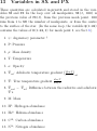
13
Variables in SX and PX
These quantities are calculated in printb and stored in the variables SX and PX. In the loop over all meshpoints, SX(J, IKK) is
the previous value of PX(J), from the previous mesh point. IKK
runs from 1 to NM, the number of meshpoints, or from the centre
to the surface of the star. (In the same loop, the variable Q(1-24)
contains the values of H(1-24,I) for mesh point I, see Sect. 6).
1. ψ: degeneracy parameter ?
2. P: Pressure
3. ρ: Mass density
4. T: Temperature
5. κ: Opacity
6. ∇ad : Adiabatic temperature gradient
7. ∇: True temperature gradient
∂ log T
∂ log P
ad
d log T
d log P
8. ∇rad − ∇ad : Difference between the radiative and adiabatic
∇’s
9. M: Mass
10. H1 : Hydrogen abundance
11. He4 : Helium abundance
12. C12 : Carbon abundance
13. N14 : Nitrogen abundance
14. O16 : Oxygen abundance
15. Ne20 : Neon abundance
16. Mg24 : Magnesium abundance
17. R: Radius
18. L: Luminosity
19. Eth : Thermal energy generation rate
20. Enuc : Nuclear energy generation rate
21. Eν : Energy loss rate in neutrinos
22. dM: Shell mass
23. Diffusion coefficient for thermohaline mixing
=
d log ρ
:
d log P
Homology invar.
25. Uhom =
d log R
:
d log P
Homology invar.
26. Vhom =
d log M
:
d log P
Homology invar.
24.
n
(n+1)
27. U: Internal energy
28. S: Entropy
29. L/Ledd : Luminosity relative to Eddington
30. wconv × l, wconv : convective velocity, l: mixing length
31. µ: Mean molecular weight
32. wt: ?
33. νe :
1
:
µ
34. νe,0 :
per free electron
1
:
µ0
per all electrons
35. wconv : convective velocity
36. M.I.: Moment of Inertia
37. φ: centrifugal-gravitational potential
38. Fm : Mass flux towards or away from the other star
39. DGOS: ∇r − ∇a + ∇OS modified Schwarzschild criterion: if
> 0: convection (but Writeup says: not used...)
40. DLRK: Heat transfer due to differential rotation
41. ∆(enth): Difference in enthalpy between star 1 and 2
42. XIK
43. V2 : ∆Φsurf between star 1 and 2
44. FAC2 ∼ V2 ?
45. FAC1 ∼ V2 ?
46. Not used
47. Not used
48. Not used
49. Not used
50. RPP: Reaction rate: pp chain effective 2p → 1/2 He4
51. RPC: Reaction rate: effective C12 + 2 p → N14
52. RPNG: Reaction rate: effective N14 + 2p → O16
53. RPN: Reaction rate: effective N14 + 2p → C12 + He4
54. RPO: Reaction rate: effective O16 + 2p → N14 + He4
55. RAN: Reaction rate: effective N14 + 3/2 He4 → Ne20
56. Cp dS/d log p
57. dL/dk
58. LQ, advection term for luminosity equation
59. ω, rotation rate
60. N 2 : Brunt-Väisälä frequency squared TODO: check this,
the code suggests it’s supposed to be the Richardson
number, but this may be incorrect
61. Ddsi mixing coefficient for the dynamical shear instability
62. Dssi mixing coefficient for the secular shear instability
63. vES velocity of Eddington-Sweet circulation
64. vµ counter term for Eddington-Sweet circultion (“µ-current”)
65. (4πr2 ρ)2 /m0 , conversion factor for diffusion coefficients CHEC
66. CHECK: SSSI? RIS?
67. TODO: ???
69. CHECK: dµ?
70. CHECK: dω?
71. CHECK: Convection + artificial mixing
72. CHECK: Thermohaline mixing
73. CHECK: Solberg-Hoiland mixing
74. CHECK: Dynamical-shear mixing
75. CHECK: Secular-shear mixing
76. CHECK: Eddington-Sweet mixing
77. CHECK: Goldberg-Schubert-Fricke mixing
14
The independent variables
The independent variables are selected in kp var in init.dat and
are also known as id(11:50), ig(11:50) in e.g. solver(). In
TWIN mode, variables (25) to (40) are the same as (1) to (16), but
for the companion star, while variables (17) to (24) are reserved for
binary parameters.
(1/25) ln f - a dimensionless quantity closely related to electron
degeneracy: for the case where electrons are non-degenerate
and non-relativistic, f ∼ 108 ρ/T 3/2
(2/26) ln T - logarithmic temperature (Kelvins)
(3/27) X16 - fractional abundance by mass of
16
O
(4/28) m - mass (1033 gm)
(5/29) X1 - the abundance of 1 H
(6/30) C - the gradient of mesh-spacing function Q(f, T, m, r)
with respect to mesh point number K. C does not vary with
K, the mesh-point number, although it varies with time. It
is in effect an eigenvalue
(7/31) ln r - logarithmic radius (1011 cm)
(8/32) L - luminosity (1033 erg/s). Not logged, because it may be
negative
(9/33) X4 - the abundance of 4 He
(10/34) X12 - the abundance of
12
20
C
For a more sophisticated binary, including mass loss, magnetic
braking, rotation (uniform but time-varying) and tidal friction, a
further 7 variables are stored:
(12/36) I - the moment of inertia of the interior material (1055 gm c
(13/37) Prot - the rotation period (days) of the star (here taken
to be independent of depth, so that it is an ‘eigenvalue’, like
C above)
(14/38) φ - the centrifugal-gravitational potential (ergs).
(15/39) φs - the potential at the surface, minus the potential on
the L1 surface (ergs); an ‘eigenvalue’.
(16/40) X14 - fractional abundance by mass of
14
N.
(17) Horb - the orbital angular momentum (1050 gm cm2 /sec); an
‘eigenvalue’.
(18) e - the eccentricity: an ‘eigenvalue’.
(19) ξ - the flux of mass towards or away from the other star (formerly F ) (1033 gm/sec); a function of depth, but zero below
the L1 surface.
(20) MB - the total mass of the binary; depleted by wind in either
or both stars, but not by mass transfer between the stars. An
‘eigenvalue’.
(22) Variable MENC for artificial, mesh-dependent energy term
(23) Variable MEA, related to MENC (Var. 22) and luminosity
...?
(24) Variable MET, related to MENC (Var. 22) . . . ?
(41) X24 - fractional abundance by mass of
24
Mg.
(42) X28 - fractional abundance by mass of
28
Si.
(43) X56 - fractional abundance by mass of
56
Fe.
(44) Total angular momentum.
15
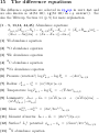
The difference equations
The difference equations are selected in kp eqn in init.dat and
are also known as id(51:90), ig(51:90) in e.g. solver(). See
also the Writeup, Section 1.5 (p. 9) for more explanation.
(1 – 5, 13,14, 44,45) Abundance equations:
σk+1/2 (Xk+1 −Xk ) − σk−1/2 (Xk −Xk−1 ) = (Ẋk +Rnuc,k )m0k −
(Xk+1 − Xk )[ṁk ] + (Xk − Xk−1 )[−ṁk+1 ]
(1) 1 H abundance equation
(2)
16
O abundance equation
(3) 4 He abundance equation
(4)
12
C abundance equation
(5)
20
Ne abundance equation
(6) Pressure (rotation?) log Pk+1 − log Pk = −(Am0 )k+1/2
2
(7) Radius: rk+1
− rk2 = (m0 /2πρr)k+1/2
(8) Temperature: log Tk+1 − log Tk = −(∇Am0 )k+1/2
(9) Luminosity: Lk+1 − Lk = (m0 E1 )k+1/2 + (m0 E2 )k [ṁk ] −
(m0 E2 )k+1 [−ṁk+1 ]
2/3
2/3
(10) Mass: mk+1 − mk
= (2m0 /3m1/3 )k+1/2
(11) Moment of inertia: Ik+1 − Ik = (2m0 r2 /3)k+1/2
(12) Surface? L1 ? potential: φk+1 − φk = (Gmm0 /4πr4 ρ)k+1/2
14
(14)
24
Mg abundance equation
(15) Sum of the abundances is constant:
instead of (14) for 24 Mg.
P
i
Ẋi = 0; normally used
(16) Equation for artificial, mesh-dependent energy term (MENC)
(18) Equation for MEA . . . ? — Related to MENC (Eq. 16) and
luminosity . . . ?
q
(19) Mass-transfer rate: ξk+1 − ξk = CMT×( [2φs ]/r m0 )k+1/2 ,
if φ > 0; = 0 otherwise.
(22) Equation for MET . . . ? — Related to MENC (Eq. 16) . . . ?
(25–37) CHECK ???
(42) Angular-momentum transport (. . . ?)
(43) Total angular momentum (. . . ?)
(44)
28
Si abundance equation
(45)
56
Fe abundance equation
16
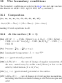
The boundary conditions
The boundary conditions are selected in kp bc in init.dat and are
also known as id(91:130), ig(91:130) in e.g. solver().
16.1
Composition
(1a, 2a, 3a, 4a, 5a, 1b, 2b, 3b, 4b, 5b)
σk±1/2 (Xk − Xk±1 ) = (Ẋk + Rnuc,k ) · (mk − mk±1 )
making 10 such equations in all.
16.2
At the surface (K = 1)
(6a) dM/dt = − CML · |ṀDDW (r, m, L, Prot )| – CMJ · |ṀJNH | –
CMR · 1.3 × 10−5 Lm/|EB | – CMS · [ln(R/RL )]3 – CMT · ξ +
CMI · M
(7c) Pressure: 23 Pgas + 34 Prad ≈ g/κ
(8c) Luminosity/temperature: L = πacr2 T 4
(9c) φ = (gravitational) potential
(10c) d(IΩ)/dt = . . ., the rate of change of angular momentum of
the star, carried away by stellar wind |ṀDDW | or lost to the
orbit by tidal friction (Ω ≡ 2π/Prot )
(11c) φs = φ: (gravitational) potential at the surface
(17c) dHorb /dt = . . ., rate of change of orbital angular momentum,
including tidal friction which exchanges AM between spin and
orbit
(18c) de/dt = . . ., rate of circularisation due to tidal friction
(20c) dMB /dt = sum of the winds from both stars; MB is the
binary mass
16.3
At the centre (K = KH)
(actually one mesh point from the centre)
(6d) m = 0
(7d) L = 0
(8d) r = 0
(9d) I = 0
(19d) ξ = 0
(13) CHECK ???
(20) CHECK ???
(25–29) CHECK ???
(30–33) CHECK ??? (2x)
(34) CHECK ???
(35) CHECK ???
(37) CHECK ???