Download The XSB System Version 2.1 Volume 1: Programmer`s Manual

The XSB System
Version 2.1
Volume 1: Programmer's Manual
xsb
Konstantinos Sagonas
Terrance Swift
David S. Warren
Juliana Freire
Prasad Rao
with contributions from
Steve Dawson
Michael Kifer
November 1999
Credits
Day-to-day care and feeding of XSB including bug xes, ports, and conguration management has been done by Kostis Sagonas, David Warren, Terrance Swift, Prasad Rao,
Steve Dawson, Juliana Freire, Baoqiu Cui and Michael Kifer.
In Version 2.1, the core engine development of the SLG-WAM has been mainly implemented by Terrance Swift, Kostis Sagonas, Prasad Rao and Juliana Freire. The breakdown, roughly, was that Terrance Swift wrote the initial tabling engine and builtins.
Prasad Rao wrote the trie-based table access routines, and Kostis Sagonas implemented
most of tabled negation. Juliana Freire revised the table scheduling mechanism starting
from Version 1.5.0 to create a more eÆcient engine, and implemented the engine for
local evaluation. Starting from XSB Version 2.0, XSB includes another tabling engine,
CHAT, which was designed and developed by Kostis Sagonas and Bart Demoen. CHAT
supports heap garbage collection (both based on a mark&slide and on a mark&copy
algorithm) which was developed and implemented by Bart Demoen and Kostis Sagonas.
Memory expansion code for WAM stacks was written by Ernie Johnson and Bart Demoen, while memory management code for CHAT areas was written by Bart Demoen
and Kostis Sagonas. Rui Marques improved the trailing of the SLG-WAM and rewrote
much of the engine to make it compliant with 64-bit architectures. Assert and retract
code was based on code written by Jiyang Xu and signicantly revised by David S.
Warren and Rui Marques. Trie assert and retract code was written by Prasad Rao.
The current version of findall/3 was re-written from scratch by Bart Demoen.
In the XSB complier, Kostis Sagonas was responsible for HiLog compilation and associated builtins. Steve Dawson implemented Unication Factoring. The auto table and
suppl table directives were written by Kostis Sagonas. The DCG expansion module
was written by Kostis Sagonas. The handling of the multifile directive was written
by Baoqiu Cui. C.R. Ramakrishnan wrote the mode analyzer for XSB. The safety check
for tabling within the scope of cuts was written by Kate Dvortsova.
Michael Kifer rewrote parts of the XSB code to make XSB congurable with GNU's
Autoconf. Harald Schroepfer helped the XSB group with the Solaris port, and Yiorgos
Adamopoulos suggested the bits to use for the HP-700 series port. Steven Dawson,
Larry B. Daniel and Franklin Chen were responsible for the MkLinux and Solaris x86
ports.
GPP, the source code preprocessor used by XSB, was written by Denis Auroux. He also
wrote the GPP manual reproduced in Appendix A.
The starting point of XSB (in 1990) was PSB-Prolog 2.0 by Jiyang Xu. PSB-Prolog in
its turn was based on SB-Prolog, primarily designed and written by Saumya Debray,
David S. Warren, and Jiyang Xu. Thanks are also due to Weidong Chen for his work
on Prolog clause indexing for SB-Prolog and to Richard O'Keefe, who contributed the
Prolog code for the Prolog reader and the C code for the tokenizer.
Contents
1 Introduction
1
2 Getting Started with XSB
5
2.1 Installing XSB under UNIX . . . . . . . . . . . . . . . . . . . . . . . . . . . . . . . .
5
2.1.1 Possible Installation Problems . . . . . . . . . . . . . . . . . . . . . . . . . . .
7
2.2 Installing XSB under Windows . . . . . . . . . . . . . . . . . . . . . . . . . . . . . .
8
2.2.1 Using Cygnus Software's CygWin32 . . . . . . . . . . . . . . . . . . . . . . .
8
2.2.2 Using Microsoft Visual C++ . . . . . . . . . . . . . . . . . . . . . . . . . . .
8
2.3 Invoking XSB . . . . . . . . . . . . . . . . . . . . . . . . . . . . . . . . . . . . . . . .
9
2.4 Compiling XSB programs . . . . . . . . . . . . . . . . . . . . . . . . . . . . . . . . . 10
2.5 Sample XSB Programs . . . . . . . . . . . . . . . . . . . . . . . . . . . . . . . . . . . 10
2.6 Exiting XSB . . . . . . . . . . . . . . . . . . . . . . . . . . . . . . . . . . . . . . . . 11
3 System Description
12
3.1 Entering and Exiting XSB . . . . . . . . . . . . . . . . . . . . . . . . . . . . . . . . . 12
3.2 The System and its Directories . . . . . . . . . . . . . . . . . . . . . . . . . . . . . . 13
3.3 The Module system of XSB . . . . . . . . . . . . . . . . . . . . . . . . . . . . . . . . 13
3.4 The Dynamic Loader and its Search Path . . . . . . . . . . . . . . . . . . . . . . . . 16
3.4.1 Changing the Default Search Path and the Packaging System . . . . . . . . . 16
3.4.2 Dynamically loading predicates in the interpreter . . . . . . . . . . . . . . . . 18
3.5 Command Line Arguments . . . . . . . . . . . . . . . . . . . . . . . . . . . . . . . . 18
3.6 Memory Management . . . . . . . . . . . . . . . . . . . . . . . . . . . . . . . . . . . 22
3.7 Compiling and Consulting . . . . . . . . . . . . . . . . . . . . . . . . . . . . . . . . . 22
3.8 The Compiler . . . . . . . . . . . . . . . . . . . . . . . . . . . . . . . . . . . . . . . . 24
3.8.1 Invoking the Compiler . . . . . . . . . . . . . . . . . . . . . . . . . . . . . . . 24
i
CONTENTS
ii
3.8.2 Compiler Options . . . . . . . . . . . . . . . . . . . . . . . . . . . . . . . . . 25
3.8.3 Specialisation . . . . . . . . . . . . . . . . . . . . . . . . . . . . . . . . . . . . 28
3.8.4 Compiler Directives . . . . . . . . . . . . . . . . . . . . . . . . . . . . . . . . 30
3.8.5 Inline Predicates . . . . . . . . . . . . . . . . . . . . . . . . . . . . . . . . . . 35
4 Syntax
36
4.1 Terms . . . . . . . . . . . . . . . . . . . . . . . . . . . . . . . . . . . . . . . . . . . . 36
4.1.1 Integers . . . . . . . . . . . . . . . . . . . . . . . . . . . . . . . . . . . . . . . 36
4.1.2 Floating-point Numbers . . . . . . . . . . . . . . . . . . . . . . . . . . . . . . 37
4.1.3 Atoms . . . . . . . . . . . . . . . . . . . . . . . . . . . . . . . . . . . . . . . . 37
4.1.4 Variables . . . . . . . . . . . . . . . . . . . . . . . . . . . . . . . . . . . . . . 38
4.1.5 Compound Terms . . . . . . . . . . . . . . . . . . . . . . . . . . . . . . . . . 38
4.1.6 Lists . . . . . . . . . . . . . . . . . . . . . . . . . . . . . . . . . . . . . . . . . 39
4.2 From HiLog to Prolog . . . . . . . . . . . . . . . . . . . . . . . . . . . . . . . . . . . 41
4.3 Operators . . . . . . . . . . . . . . . . . . . . . . . . . . . . . . . . . . . . . . . . . . 42
5 Using Tabling in XSB: A Tutorial Introduction
46
5.1 XSB as a Prolog System . . . . . . . . . . . . . . . . . . . . . . . . . . . . . . . . . . 46
5.2 Tabling in Denite Programs . . . . . . . . . . . . . . . . . . . . . . . . . . . . . . . 47
5.3 Stratied Normal Programs . . . . . . . . . . . . . . . . . . . . . . . . . . . . . . . . 52
5.3.1 Non-stratied Programs . . . . . . . . . . . . . . . . . . . . . . . . . . . . . . 54
5.3.2 On Beyond Zebra: Implementing Other Semantics for Non-stratied Programs 58
5.4 Tabled Aggregation . . . . . . . . . . . . . . . . . . . . . . . . . . . . . . . . . . . . . 60
5.4.1 Local Evaluation . . . . . . . . . . . . . . . . . . . . . . . . . . . . . . . . . . 62
6 Standard Predicates
63
6.1 Input and Output . . . . . . . . . . . . . . . . . . . . . . . . . . . . . . . . . . . . . 63
6.1.1 File Handling . . . . . . . . . . . . . . . . . . . . . . . . . . . . . . . . . . . . 63
6.1.2 Character I/O . . . . . . . . . . . . . . . . . . . . . . . . . . . . . . . . . . . 65
6.1.3 Term I/O . . . . . . . . . . . . . . . . . . . . . . . . . . . . . . . . . . . . . . 66
6.2 Special I/O . . . . . . . . . . . . . . . . . . . . . . . . . . . . . . . . . . . . . . . . . 68
6.3 Convenience . . . . . . . . . . . . . . . . . . . . . . . . . . . . . . . . . . . . . . . . . 68
6.4 Negation and Control . . . . . . . . . . . . . . . . . . . . . . . . . . . . . . . . . . . 69
CONTENTS
iii
6.5 Meta-Logical . . . . . . . . . . . . . . . . . . . . . . . . . . . . . . . . . . . . . . . . 70
6.6 All Solutions and Aggregate Predicates . . . . . . . . . . . . . . . . . . . . . . . . . . 84
6.6.1 Tabling Aggregate Predicates . . . . . . . . . . . . . . . . . . . . . . . . . . . 86
6.7 Comparison . . . . . . . . . . . . . . . . . . . . . . . . . . . . . . . . . . . . . . . . . 90
6.8 Meta-Predicates . . . . . . . . . . . . . . . . . . . . . . . . . . . . . . . . . . . . . . 93
6.9 Information about the State of the Program . . . . . . . . . . . . . . . . . . . . . . . 93
6.10 Modication of the Database . . . . . . . . . . . . . . . . . . . . . . . . . . . . . . . 104
6.11 Execution State . . . . . . . . . . . . . . . . . . . . . . . . . . . . . . . . . . . . . . . 108
6.12 Tabling . . . . . . . . . . . . . . . . . . . . . . . . . . . . . . . . . . . . . . . . . . . 112
7 Debugging
119
7.1 High-Level Tracing . . . . . . . . . . . . . . . . . . . . . . . . . . . . . . . . . . . . . 119
7.2 Low-Level Tracing . . . . . . . . . . . . . . . . . . . . . . . . . . . . . . . . . . . . . 122
8 Denite Clause Grammars
124
8.1 General Description . . . . . . . . . . . . . . . . . . . . . . . . . . . . . . . . . . . . 124
8.2 Translation of Denite Clause Grammar rules . . . . . . . . . . . . . . . . . . . . . . 125
8.3 Denite Clause Grammar predicates . . . . . . . . . . . . . . . . . . . . . . . . . . . 127
8.4 Two dierences with other Prologs . . . . . . . . . . . . . . . . . . . . . . . . . . . . 128
8.5 Interaction of Denite Clause Grammars and Tabling . . . . . . . . . . . . . . . . . 129
9 Restrictions and Current Known Bugs
131
9.1 Current Restrictions . . . . . . . . . . . . . . . . . . . . . . . . . . . . . . . . . . . . 131
9.2 Known Bugs . . . . . . . . . . . . . . . . . . . . . . . . . . . . . . . . . . . . . . . . 132
A GPP - Generic Preprocessor
134
A.1 Description . . . . . . . . . . . . . . . . . . . . . . . . . . . . . . . . . . . . . . . . . 134
A.2 Syntax . . . . . . . . . . . . . . . . . . . . . . . . . . . . . . . . . . . . . . . . . . . . 135
A.3 Options . . . . . . . . . . . . . . . . . . . . . . . . . . . . . . . . . . . . . . . . . . . 135
A.4 Syntax Specication . . . . . . . . . . . . . . . . . . . . . . . . . . . . . . . . . . . . 138
A.5 Evaluation Rules . . . . . . . . . . . . . . . . . . . . . . . . . . . . . . . . . . . . . . 141
A.6 Meta-macros . . . . . . . . . . . . . . . . . . . . . . . . . . . . . . . . . . . . . . . . 142
A.7 Examples . . . . . . . . . . . . . . . . . . . . . . . . . . . . . . . . . . . . . . . . . . 145
A.8 Advanced Examples . . . . . . . . . . . . . . . . . . . . . . . . . . . . . . . . . . . . 150
CONTENTS
iv
A.9 Author . . . . . . . . . . . . . . . . . . . . . . . . . . . . . . . . . . . . . . . . . . . . 152
B Standard Predicates and Functions
153
B.1 List of Standard Predicates . . . . . . . . . . . . . . . . . . . . . . . . . . . . . . . . 153
B.2 List of Standard Functions . . . . . . . . . . . . . . . . . . . . . . . . . . . . . . . . . 157
B.3 List of Standard Operators . . . . . . . . . . . . . . . . . . . . . . . . . . . . . . . . 158
C List of Module names
159
C.1 In syslib . . . . . . . . . . . . . . . . . . . . . . . . . . . . . . . . . . . . . . . . . . . 159
C.2 In cmplib . . . . . . . . . . . . . . . . . . . . . . . . . . . . . . . . . . . . . . . . . . 159
Chapter 1
Introduction
XSB is a research-oriented Logic Programming system for Unix and Windows-based systems. In
addition to providing all the functionality of Prolog, XSB contains several features not usually
found in Logic Programming systems, including
Evaluation according to the Well-Founded Semantics [44] through full SLG resolution;
A number of interfaces to other software systems, such a C, Java, Perl and Oracle.
Source code availability for portability and extensibility.
A compiled HiLog implementation;
A variety of indexing techniques for asserted code, along with a novel transformation technique
called unication factoring that can improve program speed and indexing for compiled code;
Extensive pattern matching libraries, which are especially useful for Web applications.
Preprosessors and Interpreters so that XSB can be used to evaluate programs that are based
on advanced formalisms, such as extended logic progams (according to the Well-Founded
Semantics [1]); Generalized Annotated Programs [23]; and F-Logic [22].
Though XSB can be used as a Prolog system1 , we avoid referring to XSB as such, because of the
availability of SLG resolution and the handling of HiLog terms. These facilities, while seemingly
simple, signicantly extend its capabilities beyond those of a typical Prolog system. We feel that
these capabilities justify viewing XSB as a new paradigm for Logic Programming.
To understand the implications of SLG resolution [8], recall that Prolog is based on a depthrst search through trees that are built using program clause resolution (SLD). As such, Prolog
is susceptible to getting lost in an innite branch of a search tree, where it may loop innitely.
SLG evaluation, available in XSB, can correctly evaluate many such logic programs. To take the
simplest of examples, any query to the program:
1
Many of the Prolog components of XSB are based on PSB-Prolog [48], which itself is based on version 2.0 of
SB-Prolog [13].
1
CHAPTER 1.
INTRODUCTION
2
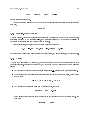
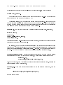
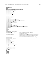
:- table ancestor/2.
ancestor(X,Y) :- ancestor(X,Z), parent(Z,Y).
ancestor(X,Y) :- parent(X,Y).
will terminate in XSB, since ancestor/2 is compiled as a tabled predicate; Prolog systems, however,
would go into an innite loop. The user can declare that SLG resolution is to be used for a predicate
by using table declarations, as here. Alternately, an auto table compiler directive can be used
to direct the system to invoke a simple static analysis to decide what predicates to table (see
Section 3.8.4). This power to solve recursive queries has proven very useful in a number of areas,
including deductive databases, language processing [24, 25], program analysis [12, 9, 5], model
checking [32] and diagnosis [34]. For eÆciency, we have implemented SLG at the abstract machine
level so that tabled predicates will be executed with the speed of compiled Prolog. We nally
note that for denite programs SLG resolution is similar to other tabling methods such as OLDT
resolution [43] (see Chapter 5 for details).
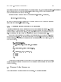
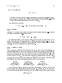
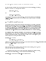
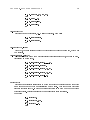
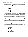
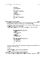
Example 1.0.1 The use of tabling also makes possible the evaluation of programs with nonstratied negation through its implementation of the well-founded semantics [44]. When logic programming rules have negation, paradoxes become possible. As an example consider one of Russell's
paradoxes | the barber in a town shaves every person who does not shave himself | written as a
logic program.
:- table shaves/2.
shaves(barber,Person):- person(Person), tnot(shaves(Person,Person)).
person(barber).
person(mayor).
Logically speaking, the meaning of this progam should be that the barber shaves the mayor, but the
case of the barber is trickier. If we conclude that the barber does not have himself our meaning does
not reect the rst rule in the program. If we conclude that the barber does shave himself, we have
reached that conclusion using information beyond what is provided in the progra. The well-founded
semantics, does not treatshaves(barber,barber) as either true or false, but as undened. Prolog,
of course, would enter an innite loop. XSB's treatment of negation is discussed further in Chapter
5.
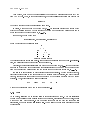
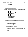
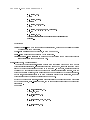
The second important extension in XSB is support of HiLog programming [6, 39]. HiLog allows a
form of higher-order programming, in which predicate \symbols" can be variable or structured. For
example, denition and execution of generic predicates like this generic transitive closure relation
are allowed:
closure(R)(X,Y) :- R(X,Y).
closure(R)(X,Y) :- R(X,Z), closure(R)(Z,Y).
where closure(R)/2 is (syntactically) a second-order predicate which, given any relation R, returns
its transitive closure relation closure(R). With XSB, support is provided for reading and writing
CHAPTER 1.
INTRODUCTION
3
HiLog terms, converting them to or from internal format as necessary (see Section 4.2). Special
meta-logical standard predicates (see Section 6.5) are also provided for inspection and handling of
HiLog terms. Unlike earlier versions of XSB (prior to version 1.3.1) the current version automatically provides full compilation of HiLog predicates. As a result, most uses of HiLog execute at
essentially the speed of compiled Prolog. For more information about the compilation scheme for
HiLog employed in XSB see [39].
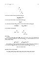
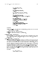
HiLog can also be used with tabling, so that the program above can also be written as:
:- table closure(_)(_,_).
closure(R)(X,Y) :- R(X,Y).
closure(R)(X,Y) :- closure(R)(X,Z), R(Z,Y).
A further goal of XSB is to provide in implementation engine for both logic programming and
for data-oriented applications such as in-memory deductive database queries and data mining [36].
One prerequisite for this functionality is the ability to load a large amount of data very quickly.
We have taken care to code in C a compiler for asserted clauses. The result is that the speed of
asserting and retracting code is faster in XSB than in any other Prolog system of which we are
aware. At the same time, because asserted code is compiled into SLG-WAM code, the speed of
executing asserted code in XSB is faster than that of many other Prologs as well. We note however,
that XSB does not follow the semantics of assert specied in [27].
Data oriented applications may also require indices other than Prolog's rst argument indexing.
XSB oers a variety of indexing techniques for asserted code. Clauses can be indexed on a groups of
arguments or on alternative arguments. For instance, the executable directive index(p/4,[3,2+1])
species indexes on the (outer functor symbol of) the third argument or on a combination of (the
outer function symbol of) the second and rst arguments. If data is expected to be structured within
function symbols and is in unit clauses, the directive index(p/4,trie) constructs an indexing trie
of the p/4 clauses using a left-to-right traversal through each clause. Representing data in this
way allows discrimination of information nested arbitrarily deep within clauses. These modes of
indexing can be combined: index(p/4,[3,2+1],trie) creates alternative trie indices beginning
with the third argument and with the second and rst argument. Using such indexing XSB can
eÆciently perform intensive analyses of in-memory knowledge bases with 1 million or so facts.
Indexing techniques for asserted code are covered in Section 6.10.
For compiled code, XSB oers unication factoring, which extends clause indexing methods
found in functional programming into the logic programming framework. Briey, unication factoring can oer not only complete indexing through non-deterministic indexing automata, but can
also factor elementary unication operations. The general technique is described in [11], and the
XSB directives needed to use it are covered in Section 3.8.
A number of interfaces are available to link XSB to other systems. In UNIX systems XSB can
be directly linked into C programs; in Windows-based system XSB can be linked into C programs
through a DLL interface. On either class of operating system, C functions can be made callable
from XSB either directly within a process, or using a socket library. XSB can access external data
in a variety of ways: through an Oracle interface, through an ODBC interface, or through a variety
of mechanisms to read data from at les. These interfaces are all described in Volume 2 of this
CHAPTER 1.
INTRODUCTION
4
manual.
Another feature of XSB is its support for extensions of normal logic programs through preprocessing libraries. Currently supported are Extended logic programs (under the well-founded
semantics), F-Logic, and Annotated Logic Programs. These libraries are described in Volume 2 of
this manual.
Source code is provided for the whole of XSB, including the engine, interfaces and supporting
functions written in C, along with the compiler, top-level interpreter and libraries written in Prolog.
It should be mentioned that we adopt some standard notational conventions, such as the
name/arity convention for describing predicates and functors, + to denote input arguments, - to
denote output arguments, ? for arguments that may be either input or output and # for arguments
that are both input and output (can be changed by the procedure). See Section 3.8.4 for more
details. Also, the manual uses UNIX syntax for les and directories except when it specically
addresses other operating systems such as Windows.
Finally, we note that XSB is under continuous development, and this document |intended to
be the user manual| reects the current status (Version 2.1) of our system. While we have taken
great eort to create a robust and eÆcient system, we would like to emphasize that XSB is also a
research system and is to some degree experimental. When the research features of XSB | tabling,
HiLog, and Indexing Techniques | are discussed in this manual, we also cite documents where they
are fully explained. All of these documents can be found via the world-wide web or anonymous ftp
from fwww/ftpg.cs.sunysb.edu, the same host from which XSB can be obtained.
While some of Version 2.1 is subject to change in future releases, we will try to be as upwardcompatible as possible. We would also like to hear from experienced users of our system about
features they would like us to include. We do try to accomodate serious users of XSB whenever we
can. Finally, we must mention that the use of undocumented features is not supported, and at the
user's own risk.
Chapter 2
Getting Started with XSB
This section describes the steps needed to install XSB under UNIX and under Windows.
2.1 Installing XSB under UNIX
If you are installing on a UNIX platform, the version of XSB that you received may not include all
the object code les so that an installation will be necessary. The easiest way to install XSB is to
use the following procedure.
1. Decide in which directory in your le system you want to install XSB and copy or move XSB
there.
2. Make sure that after you have obtained XSB by anonymous ftp (using the binary option)
or from the web, you have uncompressed it by following the instructions found in the le
README.
3. Note that after you uncompress and untar the XSB tar le, a subdirectory XSB will be tacked
on to the current directory. All XSB les will be located in that subdirectory.
In the rest of this manual, let us use $XSB DIR to refer to this subdirectory. Note the original directory structure of XSB must be maintained, namely, the directory $XSB DIR should
contain all the subdirectories and les that came with the distribution. In particular, the
following directories are required for XSB to work: emu, syslib, cmplib, lib, packages,
build, and etc.
4. Change directory to $XSB DIR/build and then run these commands:
configure
makexsb
This is it!
In addition, it is now possible to install XSB in a shared directory (e.g., /usr/local) for
everyone to use. In this situation, you should use the following sequence of commands:
5
CHAPTER 2.
GETTING STARTED WITH XSB
6
configure --prefix=$SHARED XSB
makexsb
makexsb install
where $SHARED XSB denotes the shared directory where XSB is installed. In all cases, XSB
can be run using the script
$XSB DIR/bin/xsb
However, if XSB is installed in a central location, the script for general use is:
<central-installation-directory>/<xsb-version>/bin/xsb
Important: The XSB executable determines the location of the libraries it needs based on the
full path name by which it was invoked. The \smart script" bin/xsb also uses its full path name to
determine the location of the various scripts that it needs in order to gure out the conguration
of your machine. Therefore, there are certain limitations on how XSB can be invoked.
Here are some legal ways to invoke XSB:
1. invoking the smart script bin/xsb or the XSB executable using their absolute or relative path
name.
2. using an alias for bin/xsb or the executable.
3. creating a new shell script that invokes either bin/xsb or the XSB executable using their full
path names.
Here are some ways that are guaranteed to not work in some or all cases:
1. creating a hard link to either bin/xsb or the executable and using it to invoke XSB. (Symbolic
links should be ok.)
2. changing the relative position of either bin/xsb or the XSB executable with respect to the
rest of the XSB directory tree.
Type of Machine. The congureation script automatically detects your machine and OS type,
and builds XSB accordingly. Moreover, you can build XSB for dierent architectures while
using the same tree and the same installation directory provided, of course, that these machines are sharing this directory, say using NFS or Samba. All you will have to do is to login
to a dierent machine with a dierent architecture or OS type, and repeat the above sequence
of comands.
The conguration les for dierent architectures reside in dierent directories, and there is no
danger of an architecture conict. Moreover, you can keep using the same ./bin/xsb script
regardless of the architecture. It will detect your conguration and will use the right les for
the right architecture!
CHAPTER 2.
GETTING STARTED WITH XSB
7
Choice of the C Compiler and Other options The configure script will attempt to use gcc,
if it is available. Otherwise, it will revert to cc or acc. Some versions of gcc are broken, in which case you would have to give configure an additional directive --with-cc.
If you must use some special comiler, use --with-cc=your-own-compiler. You can also
--disable-optimization (to change the default), --enable-debug, and there are many
other options. Type configure --help to see them all. Also see the le $XSB_DIR/INSTALL
for more details.
Other options are of interest to advanced users who wish to experiment with XSB, or to use
XSB for large-scale projects. In general, however users need not concern themselves with these
options.
Type of Scheduling Strategy. The ordering of operations within a tabled evaluation can dras-
tically aect its performance. XSB provides two scheduling strategies: Batched Evaluation
and Local Evaluation. Batched Evaluation is the default scheduling strategy for XSB and
evaluates queries to reduce the time to the rst answer of a query. Local Evaluation can be
chosen via the --enable-local-scheduling congure option. Detailed explanations can be
found in [18].
Type of Memory Management. Routines for managing execution stacks for tabled evaluations
can be quite complex, due to interdependencies of tabled subgoals. Indeed, memory management algorithms can be based on common elements are shared among computation states
or are copied. The default conguration of XSB shares these elements while the option
--enable-chat copies these elements. While sharing and copying have minor performance
dierences, the main reason to try the --enable-chat conguration is to use a heap garbage
collector that has been written for it. See [35, 14, 15, 16] for in-depth discussion of the engine
memory management.
2.1.1 Possible Installation Problems
Lack of Space for Optimized Compilation of C Code When making the optimized version
of the emulator, the temporary space available to the C compiler for intermediate les is sometimes
not suÆcient. For example on one of our SPARCstations that had very little /tmp space the "-O4"
option could not be used for the compilation of les emuloop.c, and tries.c, without changing the
default tmp directory and increasing the swap space. Depending on your C compiler, the amount
and nature of /tmp and swap space of your machine you may or may not encounter problems. If
you are using the SUN C compiler, and have disk space in one of your directories, say dir, add the
following option to the entries of any les that cannot be compiled:
-temp=dir
If you are using the GNU C compiler, consult its manual pages to nd out how you can change
the default tmp directory or how you can use pipes to avoid the use of temporary space during
compiling. Usually changing the default directory can be done by declaring/modifying the TMPDIR
environment variable as follows:
setenv TMPDIR dir
CHAPTER 2.
GETTING STARTED WITH XSB
8
Missing XSB Object Files When an object (*.O) le is missing from the lib directories you
can normally run the make command in that directory to restore it (instructions for doing so are
given in Chapter 2). However, to restore an object le in the directories syslib and cmplib, one
needs to have a separate Prolog compiler accessible (such as a separate copy of XSB), because the
XSB compiler uses most of the les in these two directories and hence will not function when some
of them are missing. For this reason, distributed versions normally include all the object les in
syslib and cmplib.
2.2 Installing XSB under Windows
2.2.1 Using Cygnus Software's CygWin32
This is easy: just follow the Unix instructions. This is the preferred way to run XSB under
Windows, because this ensures that all features of XSB are available.
2.2.2 Using Microsoft Visual C++
1. XSB will unpack into a subdirectory named xsb. Assuming that you have XSB.ZIP in the
$XSB DIR directory, you can issue the command
unzip386 xsb.zip
which will install XSB in the subdirectory xsb.
2. If you decide to move XSB to some other place, make sure that the entire directory tree is
moved | XSB executable looks for the les it needs relatively to its current position in the
le system.
You can compile XSB under Microsoft Visual C++ compiler to create a console-supported top
loop or a DLL by following these steps:
1. cd build
2. Type:
makexsb wind "CFG=option" ["DLL=yes"] ["ORACLE=yes"] ["SITE LIBS=libraries"]
The items in square brackets are optional.
The options for CFG are: release or debug. The latter is used when you want to compile
XSB with debugging enabled.
The other parameters to makexsb wind are optional. The DLL parameter tells Visual
C++ to compile XSB as a DLL. The ORACLE parameter compiles XSB with support
for Oracle DBMS. If ORACLE is specied, you must also specify the necessary Oracle
libraries using the parameter SITE LIBS.
CHAPTER 2.
GETTING STARTED WITH XSB
9
3. The above command will compile XSB as requested and will put the XSB executable in:
$XSB DIRnconfignx86-pc-windowsnbinnxsb:exe
If you requested to compile XSB as a DLL, then the DLL will be placed in
$XSB DIRnconfignx86-pc-windowsnbinnxsb:dll
Note: the XSB executable and the DLL can coexist in the same source tree structure. However,
if you rst compiled XSB as an executable and then want to compile it as a DLL (or vice versa),
then you must run
makexsb_wind clean
in between.
2.3 Invoking XSB
Under Unix, XSB can be invoked by the command:
$XSB DIR/bin/xsb
if you have installed XSB in your private directory. If XSB is instaled in a shared directory (e.g.,
$SHARED XSB for the entire site (UNIX only), then you should use
$SHARED XSB/bin/xsb
In both cases, you will nd yourself in the top level interpreter. As mentioned above, this script
automatically detects the system conguration you are running on and will use the right les and
executables. (Of course, XSB should have been built for that architecture earlier.)
Under Windows, you should invoke XSB by typing:
$XSB DIRnconfignx86-pc-windowsnbinnxsb:exe
You may want to make an alias such as xsb to the above commands, for convenience, or you
might want to put the directory where the XSB command is found in the $PATH environment
variable. However, you should not make hard links to this script or to the XSB executable. If you
invoke XSB via such a hard link, XSB will likely be confused and will not nd its libraries. That
said, you can create other scripts and cal the above script from there.
Most of the \standard" Prolog predicates are supported by XSB, so those of you who consider
yourselves champion entomologists, can try to test them for bugs now. Details are in Chapter 6.
CHAPTER 2.
10
GETTING STARTED WITH XSB
2.4 Compiling XSB programs
All source programs should be in les whose names have the suÆx .P. One of the ways to compile
a program from a le in the current directory and load it into memory, is to type the query:
[my_file].
where my_file is the name of the le, or preferably, the name of the module (obtained from the
le name by deleting the suÆx .P). To nd more about the module system of XSB see Section 3.3.
If you are eccentric (or you don't know how to use an editor) you can also compile and load
predicates input directly from the terminal by using the command:
[user].
A CTRL-d or the atom end_of_file followed by a period terminates the input stream.
2.5 Sample XSB Programs
If for some reason you don't feel like writing your own XSB programs, there are several sample
XSB programs in the directory: $XSB DIR/examples. All contain source code.
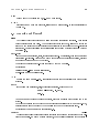
The entry predicates of all the programs in that directory are given the names demo/0 (which
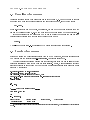
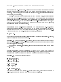
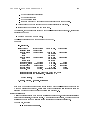
prints out results) and go/0 (which does not print results).1 Hence, a sample session might look
like (the actual times shown below may vary and some extra information is given using comments
after the % character):
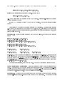
my_favourite_prompt> cd $XSB_DIR/examples
my_favourite_prompt> $XSB_DIR/bin/xsb
XSB Version 2.0 (Gouden Carolus) of June 27, 1999
[i586-pc-linux-gnu; mode: optimal; engine: slg-wam; scheduling: batched]
| ?- [queens].
[queens loaded]
yes
| ?- demo.
% ...... output from queens program .......
Time used: 0.4810 sec
yes
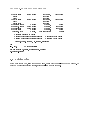
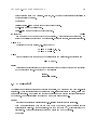
| ?- statistics.
memory (total)
permanent space
1
1906488 bytes:
202552 bytes
203452 in use,
1703036 free
This convention does not apply to the subdirectories of the examples directory, which illustrate advanced features
of XSB.
CHAPTER 2.
glob/loc space
global
local
trail/cp space
trail
choice point
SLG subgoal space
SLG unific. space
SLG completion
SLG trie space
(call+ret. trie
786432 bytes:
786432 bytes:
0
65536
65536
0
0
bytes:
bytes:
bytes:
bytes:
bytes,
432 in use,
240 bytes
192 bytes
468 in use,
132 bytes
336 bytes
0 in use,
0 in use,
0 in use,
0 in use,
trie hash tables
0 subgoals currently in tables
0 subgoal check/insert attempts inserted
0 answer check/insert attempts inserted
Time: 0.610 sec. cputime,
yes
| ?- halt.
11
GETTING STARTED WITH XSB
786000 free
785964 free
0
65536
65536
0
0
free
free
free
free
bytes)
0 subgoals in the tables
0 answers in the tables
18.048 sec. elapsetime
% I had enough !!!
End XSB (cputime 1.19 secs, elapsetime 270.25 secs)
my_favourite_prompt>
2.6 Exiting XSB
If you want to exit XSB, issue the command halt. or simply type CTRL-d at the XSB prompt. To
exit XSB while it is executing queries, strike CTRL-c a number of times.
Chapter 3
System Description
Throughout this chapter, we use $XSB_DIR to refer to the directory in which XSB was installed.
3.1 Entering and Exiting XSB
After the system has been installed, the emulator's executable code appears in the le:
$XSB_DIR/bin/xsb
or, if, after being built, XSB is later installed at a central location, $SHARED_XSB.
$SHARED_XSB/bin/xsb
and indeed, using this command, invokes XSB's top level interpreter which is the usual way of
using XSB
Version 2.1 of XSB can also directly execute object code les from the command line interface.
Suppose you have a top-level routine go in a le foo.P that you would like to run from the UNIX or
Windows command line. As long as foo.P contains a directive :- go., and foo has been compiled
to an object le (foo.O), then
$XSB_DIR/bin/xsb -B foo.O
will execute go, loading the appropriate les as needed. In fact the command $XSB_DIR/bin/xsb
is equivalent to the command:
$XSB_DIR/bin/xsb -B $XSB_DIR/syslib/loader.O
There are several ways to exit XSB. A user may issue the command halt. or end_of_file,
or simply type CTRL-d at the XSB prompt. To interrupt XSB while it is executing a query, strike
CTRL-c.
12
CHAPTER 3.
SYSTEM DESCRIPTION
13
3.2 The System and its Directories
The XSB system, when installed, resides in a single directory that contains the following subdirectories:
1. build
2. docs
3. emu
4. etc
5. examples
6. cmplib
7. lib
8. packages
9. syslib
The directory emu contains the source and object code for the XSB emulator, which is written
in C.
The directories syslib, cmplib and lib contain source and object code for the basic Prolog
libraries, the compiler, and the extended Prolog libraries, respectively. All the source programs
are written in XSB, and all object (byte code) les contain SLG-WAM instructions that can be
executed by the emulator. These byte-coded instructions are machine-independent, so usually no
installation procedure is needed for the byte code les.
The directory packages contains the various applications, written in XSB, which are not part
of the system per se.
You must already be familiar with the build directory, which is what you must have used
to build XSB. This directory contains XSB conguration scripts. The directory etc contains
miscellaneous les used by XSB.
The directory docs contains this manual in LATEX, dvi and Postscipt format, and the directory
examples contains sample programs to demonstrate various features of XSB.
3.3 The Module system of XSB
XSB has been designed as a module-oriented Prolog system. Modules provide a small step towards
logic programming \in the large" that facilitates large programs or projects to be put together from
components which can be developed, compiled and tested separately. Also module systems enforce
the principle of information hiding and can provide a basis for data abstraction.
CHAPTER 3.
SYSTEM DESCRIPTION
14
The module system of XSB, unlike the module systems of most other Prolog systems is atombased. Briey, the main dierence between atom-based module systems and predicate-based ones
is that in an atom-based module system any symbol in a module can be imported, exported or be
a local symbol as opposed to the predicate-based ones where this can be done only for predicate
symbols 1 .
Usually the following three les are associated with a particular module:
A single source le, whose name is the module name plus the suÆx \.P".
An optional header le, whose name is the module name plus the suÆx \.H".
An object (byte-code) le, whose name consists of the module name plus the suÆx \.O".
The header le is normally used to contain declarations and directives while the source le usually
contains the actual denitions of the predicates dened in that module. The module hierarchy of
XSB is therefore at | nested modules are not possible.
In order for a le to be a module, it should contain one or more export declarations, which
specify that a set of symbols appearing in that module is visible and therefore can be used by any
other module. A module can also contain local declarations, which specify that a set of symbols are
visible by this module only, and therefore cannot be accessed by any other module. Any le (either
module or not) may also contain import declarations, which allow symbols dened in and exported
by other modules to be used in the current module. We note that only exported symbols can be
imported; for example importing a local symbol will cause an environment conflict error.
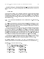
Export, local, and import declarations can appear anywhere in the source or header les and
have the following forms:
sym1, ..., syml .
:- local sym1 , ..., symm .
:- import sym1 , ..., symn from module.
where symi has the form functor=arity.
:- export
If the user does not want to use modules, he can simply bypass the module system by not
supplying any export declarations. Such exportless les (non-modules) will be loaded into the
module usermod, which is the working module of the XSB interpreter.
Currently the module name is stored in its byte code le, which means that if the byte code
le is renamed, the module name is not altered, and hence may cause confusion to the user and/or
the system. So, it is advisable that the user not rename byte code les generated for modules by
the XSB compiler. However, byte code les generated for non-modules can be safely renamed. We
will try to x the problem described above in future releases.
In order to understand the semantics of modules, the user should keep in mind that in a module
oriented system, the name of each symbol is identied as if it were prexed with its module name,
1
Operator symbols can be exported as any other symbols, but their precedence must be redeclared in the importing
module.
CHAPTER 3.
SYSTEM DESCRIPTION
15
hence two symbols of the same functor=arity but dierent module prexes are distinct symbols.
Currently the following set of rules is used to determine the module prex of a symbol:
Every predicate symbol appearing in a module (i.e. that appears as the head of some clause)
is assumed to be local to that module unless it is declared otherwise (via an export or import
declaration). Symbols that are local to a given module are not visible to other modules.
Every other symbol (essentially function symbols) in a module is assumed to be global (its
module prex is usermod) unless declared otherwise.
If a symbol is imported from another module (via an explicit import declaration), the module
prex of the symbol is the module it is imported from; any other symbol takes the module
where the symbol occurs as its module prex.
The XSB interpreter is entered with usermod as its working module.
Symbols that are either dened in non-modules loaded into the system or that are dynamically
created (by the use of standard predicates such as read/1, functor/3, '=..'/2, etc) are
contained in usermod.
The following facts about the module system of XSB may not be immediately obvious:
If users want to use a symbol from another module, they must explicitly import it otherwise
the two symbols are dierent even if they are of the same functor=arity form.
A module can only export predicate symbols that are dened in that module. As a consequence, a module cannot export predicate symbols that are imported from other modules.
This happens because an import declaration is just a request for permission to use a symbol
from a module where its denition and an export declaration appear.
The implicit module for a particular symbol appearing in a module must be uniquely determined. As a consequence, a symbol of a specic functor=arity cannot be declared as both
exported and local, or both exported and imported from another module, or declared to be
imported from more than one module, etc. These types of environment conicts are detected
at compile-time and abort the compilation.
It is an error to import a symbol from a module that does not export it. This error is not
detected at compile-time but at run-time when a call to that symbol is made. If the symbol
is dened in, but not exported from the module that denes it, an environment conict error
will take place. If the symbol is not dened in that module an undened predicate/function
error will be be reported to the user.
In the current implementation, at any time only one symbol of a specic functor=arity form
can appear in a module. As an immediate consequence of this fact, only one functor=arity
symbol can be loaded into the current working module (usermod). An attempt to load a
module that redenes that symbol results in a warning to the user and the newly loaded
symbol overrides the denition of the previously loaded one.
CHAPTER 3.
SYSTEM DESCRIPTION
16
3.4 The Dynamic Loader and its Search Path
The dynamic (or automatic) loader comprises one of XSB's dierences from other Prolog systems.
In XSB, the loading of user modules Prolog libraries (including the XSB compiler itself) is delayed
until predicates in them are actually needed, saving program space for large Prolog applications.
The delay in the loading is done automatically, unlike other systems where it must be explicitly
specied for non-system libraries.
When a predicate imported from another module (see section 3.3) is called during execution,
the dynamic loader is invoked automatically if the module is not yet loaded into the system, The
default action of the dynamic loader is to search for the byte code le of the module rst in the
system library directories (in the order lib, syslib, and then cmplib), and nally in the current
working directory. If the module is found in one of these directories, then it will be loaded (on
a rst-found basis). Otherwise, an error message will be displayed on the current output stream
reporting that the module was not found.
In fact, XSB loads the compiler and most system modules this way. Because of dynamic loading,
the time it takes to compile a le is slightly longer than usual the rst time the compiler is invoked
in a session.
3.4.1 Changing the Default Search Path and the Packaging System
Users are allowed to supply their own library directories and also to override the default search
path of the dynamic loader. User-supplied library directories are searched by the dynamic loader
before searching the default library directories.
The default search path of the dynamic loader can easily be changed by having a le named
.xsb/xsbrc.P in the user's home directory. The .xsb/xsbrc.P le, which is automatically consulted by the XSB interpreter, might look like the following:
::::-
assert(library_directory('./')).
assert(library_directory('~/')).
assert(library_directory('~my_friend')).
assert(library_directory('/usr/lib/sbprolog')).
After loading the module of the above example, the current working directory is searched rst
(as opposed to the default action of searching it last). Also, XSB's system library directories
(lib, syslib, and cmplib), will now be searched after searching the user's, my friend's and the
"/usr/lib/sbprolog/" directory.
In fact, XSB also uses library directory/1 for internal purposes. For instance, before the
user's .xsb/xsbrc.P is consulted, XSB puts the packages directory and the directory
.xsb/config/$CONFIGURATION
on the library search path. The directory .xsb/config/$CONFIGURATION is used to store user
libraries that are machine or OS dependent. ($CONFIGURATION for a machine is something that
CHAPTER 3.
SYSTEM DESCRIPTION
17
looks like sparc-sun-solaris2.6 or pc-linux-gnu, and is selected by XSB automatically at run
time).
Note that the le .xsb/xsbrc.P is not limited to setting the library search path. In fact,
arbitrary Prolog code can go there.
We emphasize that in the presense of a .xsb/xsbrc.P le it is the user's responsibility to avoid
module name clashes with modules in XSB's system library directories. Such name clashes can
cause the system to behave strangely since these modules will probably have dierent semantics
from that expected by the XSB system code. The list of module names in XSB's system library
directories can be found in appendix C.
Apart from the user libraries, XSB now has a simple packaging system. A package is an application consisting of one or more les that are organized in a subdirectory of one of the XSB system
or user libraries. The system directory $XSB_DIR/packages has several examples of such packages.
Packages are convenient as a means of organizing large XSB applications, and for simplifying user
interaction with such applications. User-level packaging is implemented through the predicate
bootstrap_userpackage(+LibraryDir, +PackageDir, +PackageName).
which must be imported from the packaging module.
To illustrate, suppose you wanted to create a package, foobar, inside your own library, my lib.
Here is a sequence of steps you can follow:
1. Make sure that my lib is on the library search path by putting an appropriate assert statement
in your xsbrc.P.
2. Make subdirectory ~/my_lib/foobar and organize all the package les there. Designate one
le, say, foo.P, as the entry point, i.e., the application le that must be loaded rst.
3. Create the interface program ~/my_lib/foobar.P with the following content:
:- bootstrap_userpackage('~/my_lib', 'foobar', foobar), [foo].
The interface program and the package directory do not need to have the same name, but it
is convenient to follow the above naming schema.
4. Now, if you need to invoke the foobar application, you can simply type [foobar]. at the
XSB prompt. This is because both and ~/my_lib/foobar have already been automatically
added to the library search path.
5. If your application les export many predicates, you can simplify the use of your package by
having ~/my_lib/foobar.P import all these predicates, renaming them, and then exporting
them. This provides a uniform interface to the foobar module, since all the package predicates
are can now be imported from just one module, foobar.
CHAPTER 3.
SYSTEM DESCRIPTION
18
In addition to adding the appropriate directory to the library search path, the predicate bootstrap_userpackage/3
also adds information to the predicate package_configuration/3, so that other applications could
query the information about loaded packages.
Packages can also be unloaded using the predicate unload_package/1. For instance,
:- unload_package(foobar).
removes the directory ~/my_lib/foobar from the library search path and deletes the associated
information from package_configuration/3.
3.4.2 Dynamically loading predicates in the interpreter
Modules are usually loaded into an environment when they are consulted (see section 3.7). Specic
predicates from a module can also be imported into the run-time environment through the standard
predicate import PredList from Module. Here, PredList can either be a Prolog list or a comma
list. (The import/1 can also be used as a directive in a source module (see section 3.3).
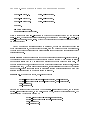
We provide a sample session for compiling, dynamically loading, and querying a user-dened
module named quick sort. For this example we assume that quick sort is a le in the current
working directory, and contains the denitions of the predicates concat/3 and qsort/2, both of
which are exported.
| ?- compile(quick_sort).
[Compiling ./quick_sort]
[quick_sort compiled, cpu time used: 1.439 seconds]
yes
| ?- import concat/3, qsort/2 from quick_sort.
yes
| ?- concat([1,3], [2], L), qsort(L, S).
L = [1,3,2]
S = [1,2,3]
yes.
The standard predicate import/1 does not load the module containing the imported predicates,
but simply informs the system where it can nd the denition of the predicate when (and if) the
predicate is called.
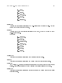
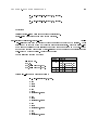
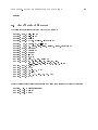
3.5 Command Line Arguments
There are several command line options for the emulator. The general synopsis is:
CHAPTER 3.
xsb
xsb
xsb
xsb
xsb
xsb
SYSTEM DESCRIPTION
19
xsb [flags] [-l] [-i]
[flags] -n
[flags] module
[flags] -B boot_module [-D cmd_loop_driver] [-t] [-e goal]
[flags] -B module_to_disassemble -d
-[h | v]
--help | --version | --nobanner | --quietload | --noprompt
memory management flags:
-c tcpsize | -m glsize | -o complsize | -u pdlsize | -r | -g gc_type
miscellaneous flags:
-s | -T
module:
Module to execute after XSB starts up.
Module should have no suffixes, no directory part, and
the file module.O must be on the library search path.
boot_module:
This is a developer's option.
The -B flags tells XSB which bootstraping module to use instead
of the standard loader. The loader must be specified using its
full pathname, and boot_module.O must exist.
module_to_disassemble:
This is a developer's option.
The -d flag tells XSB to act as a disassembler.
The -B flag specifies the module to disassemble.
cmd_loop_driver:
The top-level command loop driver to be used instead of the
standard one. Usually needed when XSB is run as a server.
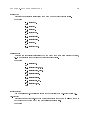
-i : bring up the XSB interpreter
-e goal : evaluate goal when XSB starts up
-l : the interpreter prints unbound variables using letters
-n : used when calling XSB from C
-B : specify the boot module to use in lieu of the standard loader
-D : Sets top-level command loop driver to replace the default.
-t : trace execution at the SLG-WAM instruction level
(for this to work, build XSB with the --debug option)
-d : disassemble the loader and exit
-c N : allocate N KB for the trail/choice-point stack
-m N : allocate N KB for the local/global stack
-o N : allocate N KB for the SLG completion stackof
-u N : allocate N KB for the SLG unification (table copy) stack
-r : turn off automatic stack expansion
-g gc_type : choose the garbage collection ("none", "sliding", or "copying")
CHAPTER 3.
SYSTEM DESCRIPTION
20
-s : maintains more detailed statistical information
-T : print a trace of each called predicate
-v, --version : print the version and configuration information about XSB.
-h, --help : print this help message
--nobanner : don't show the XSB banner on startup
--quietload : don't show the `module loaded' messages
--noprompt : don't show prompt (for non-interactive use)
The order in which these options appear makes no dierence.
-i Brings up the XSB interpreter. This is the normal use and because of this, use of this option is
optional and is only kept for backwards compatibility.
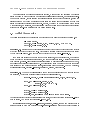
-l Forces the interpreter to print unbound variables as letters, as opposed to the default setting
which prints variables as memory locations prexed with an underscore. For example, starting
XSB's interpreter with this option will print the following:
| ?- Y = X, Z = 3, W = foo(X,Z).
Y
X
Z
W
=
=
=
=
A
A
3
foo(A,3)
as opposed to something like the following:
| ?- Y = X, Z = 3, W = foo(X,Z).
Y
X
Z
W
=
=
=
=
_10073976
_10073976
3
foo(_10073976,3);
-n used in conjunction with the -i option, to indicate that the usual read-eval-print top-loop is
not to be entered, but instead will interface to a calling C program. See the chapter Calling
XSB from C in Volume 2 for details.
-d Produces a disassembled dump of byte code file to stdout and exits.
-c size Allocates initial size Kbytes of space to the trail/choice-point stack area. The trail stack
grows upward from the bottom of the region, and the choice point stack grows downward
from the top of the region. Because this region is expanded automatically from Version 1.6.0
onward, this option should rarely need to be used. Default initial size: 768 Kbytes.
-m size Allocates size Kbytes of space to the local/global stack area. The global stack grows
upward from the bottom of the region, and the local stack grows downward from the top of
the region. Default: 768 Kbytes.
CHAPTER 3.
SYSTEM DESCRIPTION
21
-o size Allocates size Kbytes of space to thecompletion stack area. Because this region is expanded
automatically from Version 1.6.0 onward, this option should rarely need to be used. Default
initial size 64 Kbytes.
-u size Allocates size Kbytes of space to the unication (and table copy) stack. Default 64 Kbytes.
(This option should rarely need to be used).
-D Tells XSB to use a top-level command loop driver specied here instead of the standard XSB
interpreter. This is most useful when XSB is used as a server.
-r Turns o automatic stack expansion.
-g gc type Chooses the garbage collection strategy that is employed; choice of the strategy is
between "none" (meaning perform no garbage collection), or garbage collection based on
"sliding" or on "copying". Since garbage collection is only available when the emulator is
based on a CHAT model (see also the installation options), this option only makes sense in
this context; it is ineective when the emulator is SLG-WAM based.
-s Maintains information on the size of program stacks for the predicate statistics/0. This
option may be expected to slow execution by around 10%. Default: o.
-T Generates a trace at entry to each called predicate (both system and user-dened). This option
is available mainly for people who want to modify and/or extend XSB, and it is not the normal
way to trace XSB programs. For the latter, the builtin predicates trace/0 or debug/0 should
be used (see Chapter 7).
Note: This option is not available when the system is being used at the non-tracing mode
(see Section 7).
-t Traces through code at SLG-WAM instruction level. This option is for internal debugging and
is not fully supported. It is also not available when the system is being used at the non-debug
mode (see Section 7).
-e goal Pass goal to XSB at starup. This goal is evaluated right before the rst prompt is issued.
For instance, xsb -e "write(Hello!'), nl."' will print a heart-warming message when XSB
starts up.
--nobanner Start XSb without showing the startup banner. Useful in batch scripts and for inter-
process communication (when XSB is launched as a subprocess).
--quietload Do not tell when a new module gets loaded. Again, is useful in non-interactive
activities and for interprocess communication.
--noprompt Do not show te XSB prompt. This is useful only in batch mode and in interprocess
communication when you do not want the prompt to clutter the picture.
As an example, a program which uses more heap and local stack than the default conguration
of XSB might be run by invoking XSB with the command.
xsb -m 2000
CHAPTER 3.
SYSTEM DESCRIPTION
22
3.6 Memory Management
All execution stacks are automatically expenaded in Version 2.1 including the local stack/heap
region, the trail/choice point region and the completion stack region. Each of these regions begin
with an initial value set by the user (or the default stated in Section 3.5), and double their size
until it is not possible to do so with available system memory. At that point XSB tries to nd the
maximal amount of space that will still t in system memory. Garbage collection is automatically
performed for retracted clauses. In addition, heap garbage collection is automatically included
when the --enable-chat conguration option is used.
The program area (the area into which the code is loaded) is also dynamically expanded as
needed, and the area occupied by dynamic code (created using assert/1, or the standard predicate
load dyn/1) is reclaimed when that code is retracted. Version 1.8 improves memory management
for retracted dynamic code.
Version 2.1 provides memory management for table space as well. Space for tables is dynamically allocated as needed and reclaimed through use of the predicate abolish all tables/0 (see
Section 6.12).
3.7 Compiling and Consulting
In XSB, both compiled and interpreted code are transformed into SLG-WAM instructions. The
main dierences are that compiled code may be more optimized than interpreted code, and that
compilation produces an object code le.
This section describes the actions of the standard predicate consult/[1,2] (and of reconsult/[1,2]
which is dened to have the same actions as consult/[1,2]). consult/[1,2] is the most convenient method for entering rules into XSB's database. Though consult comes in many avors, the
most general form is:
consult(+FileList, +CompilerOptionList)
At the time of the call both of its arguments should be instantiated (ground). FileList is a list of
lenames or module names (see section 3.3) and CompilerOptionList is a list of options that are
to be passed to the compiler when (and if) it should be invoked. For a detailed description of the
format and the options that can appear in this list see Section 3.8.
If the user wants to consult one module (le) only, she can provide an atom instead of a list
for the rst argument of consult/2. Furthermore, if there isn't any need for special compilation
options the following two forms:
[FileName].
consult(FileName).
are just notational shorthands for:
consult(FileName, []).
CHAPTER 3.
SYSTEM DESCRIPTION
23
Consulting a module (le) generally consists of the following ve steps which are described in
detail in the next paragraphs.
Name Resolution : determine the module to be consulted.
Compilation : if necessary (and the source le is not too big), compile the module using predicate
compile/2 with the options specied.
Loading load the object code of the module into memory.
Importing import all the exported predicates of that module to the current working module
(usermod).
Query Execution : execute any queries that the module may contain.
There are two steps to name resolution: determination of the proper directory prex and
determination of the proper extension. When FileName is absolute (i.e. in UNIX contains a slash
'/') determination of the proper directory prex is straightforward. However, the user may also
enter a name without any directory prex. In this case, the directory prex is a directory in the
dynamic loader path (see section 3.4) where the source le exists. Once the directory prex is
determined, the le name is checked for an extension. If there is no extension the loader rst
checks for a le in the directory with the .P extension, (or .c for foreign modules) before searching
for a le without the extension. Note that since directories in the dynamic loader path are searched
in a predetermined order (see section 3.4), if the same le name appears in more than one of these
directories, the compiler will consult the rst one it encounters.
Compilation is performed if the update date of the the source le (*.P) is later than that of the
the object le (*.O), and if the source le is not larger than the default compile size. This default
compile is set to be 20,000 bytes (in cmplib/config.P), but can be reset by the user. If the source
le is larger than the default compile size, the le will be loaded using load dyn/1, and otherwise
it will be compiled (load dyn/1 can also be called separately, see the section Asserting Dynamic
Code for details. While load dyn gives reasonibly good execution times, compilation can always
be done by using compile/[1,2] explicitly. Currently (Version 2.1), a foreign language module is
compiled when at least one of les *.c or *.H has been changed from the time the corresponding
object les have been created.
Whether the le is compiled or dynamically loaded, the byte-code for the le is loaded into
XSB's database. The default action upon loading is to delete any previous byte-code for predicates
dened in the le. If this is not the desired behavior, the user may add to the le a declaration
:- multifile <Predicate List> .
where Predicate List is a list of predicates in functor/arity form. The eect of this declaration
is to delete only those clauses of predicate/arity that were dened in the le itself.
After loading the module, all exported predicates of that module are imported into the current environment (the current working module usermod). For non-modules (see Section 3.3), all
predicates are imported into the current working module.
CHAPTER 3.
SYSTEM DESCRIPTION
24
Finally any queries | that is, any terms with principal functor ':-'/1 that are not directives
like the ones described in Section 3.8 | are executed in the order that they are encountered.
3.8 The Compiler
The XSB compiler translates XSB source les into byte-code object les. It is written entirely
in Prolog. Both the sources and the byte code for the compiler can be found in the XSB system
directory cmplib.
Prior to compiling, XSB lters the programs through GPP, a preprocessor written by Denis
Auroux ([email protected]). This preprocessor maintains high degree of compatibility
with the C preprocessor, but is more suitable for processing Prolog programs. The preprocessor
is invoked with the compiler option xpp_on as described below. The various features of GPP are
described in Appendix A.
XSB also allows the programmer to use preprocessors other than GPP. However, the modules
that come with XSB distribution require GPP. This is explained below (see xpp_on compiler option).
The following sections describe the various aspects of the compiler in more detail.
3.8.1 Invoking the Compiler
The compiler is invoked directly at the interpreter level (or in a program) through the Prolog
predicates compile/[1,2].
The general forms of predicate compile/2 are:
compile(+File, +OptionList)
compile(+FileList, +OptionList)
and at the time of the call both of its arguments should be ground.
The second form allows the user to supply a proper list of le names as the parameter for
compile/[1,2]. In this case the compiler will compile all the les in FileList with the compiler
options specied in OptionList (but see Section 3.8.2 below for the precise details.)
j
?- compile(Files).
is just a notational shorthand for the query:
j
?- compile(Files, []).
The standard predicates consult/[1,2] call compile/1 (if necessary). Argument File can be
any syntactically valid UNIX or Windows le name (in the form of a Prolog atom), but the user
can also supply a module name.
The list of compiler options OptionList, if specied, should be a proper Prolog list, i.e. a term
of the form:
[
option1 , option2 , : : :, optionn ].
CHAPTER 3.
SYSTEM DESCRIPTION
25
where optioni is one of the options described in Section 3.8.2.
The source le name corresponding to a given module is obtained by concatenating a directory
prex and the extension .P (or .c) to the module name. The directory prex must be in the
dynamic loader path (see Section 3.4). Note that these directories are searched in a predetermined
order (see Section 3.4), so if a module with the same name appears in more than one of the
directories searched, the compiler will compile the rst one it encounters. In such a case, the user
can override the search order by providing an absolute path name.
If File contains no extension, an attempt is made to compile the le File.P (or File.c) before
trying compiling the le with name File.
We recommend use of the extension .P for Prolog source le to avoid ambiguity. Optionally,
users can also provide a header le for a module (denoted by the module name suÆxed by .H).
In such a case, the XSB compiler will rst read the header le (if it exists), and then the source
le. Currently the compiler makes no special treatment of header les. They are simply included
in the beginning of the corresponding source les, and code can, in principle, be placed in either.
In future versions of XSB the header les may be used to check interfaces across modules, hence it
is a good programming practice to restrict header les to declarations alone.
The result of the compilation (an SLG-WAM object code le) is stored in a (hlenamei.O), but
compile/[1,2] does not load the object le it creates. (The standard predicates consult/[1,2]
and reconsult/[1,2] both recompile the source le, if needed, and load the object le into the
system.) The object le created is always written into the directory where the source le resides
(the user should therefore have write permission in that directory).
If desired, when compiling a module (le), clauses and directives can be transformed as they
are read. This is indeed the case for denite clause grammar rules (see Chapter 8), but it can
also be done for clauses of any form by providing a denition for predicate term expansion/2 (see
Section 8.3).
Predicates compile/[1,2] can also be used to compile foreign language modules. In this case,
the names of the source les should have the extension .c and a .P le must not exist. A header
le (with extension .H) must be present for a foreign language module (see the chapter Foreign
Language Interface in Volume 2.
3.8.2 Compiler Options
Compiler options can be set in three ways: from a global list of options (see set global compiler options/1),
from the compilation command (see compile/2 and consult/2), and from a directive in the le to
be compiled (see compiler directive compiler options/1).
set global compiler options(+OptionsList)
OptionsList is a list of compiler options (described below). Each can optionally be prexed
by + or -, indicating that the option is to be turned on, or o, respectively. (No prex turns
the option on.) This evaluable predicate sets the global compiler options in the way indicated.
These options will be used in any subsequent compilation, unless reset by another call to this
predicate, or overridden by options provided in the compile invocation, or overridden by
CHAPTER 3.
SYSTEM DESCRIPTION
26
options in the le to be compiled.
The following options are currently recognized by the compiler:
optimize When specied, the compiler tries to optimize the object code. In Version 2.1, this option
optimizes predicate calls, among other features, so execution may be considerably faster for
recursive loops. However, due to the nature of the optimizations, the user may not be able
to trace all calls to predicates in the program. Also the Prolog code should be static. In
other words, the user is not allowed to alter the entry point of these compiled predicates by
asserting new clauses. As expected, the compilation phase will also be slightly longer. For
these reasons, the use of the optimize option may not be suitable for the development phase,
but is recommended once the code has been debugged.
xpp on Filter the program through a preprocessor before sending it to the XSB compiler. By
default (and for the XSB code itself), XSB uses GPP, a preprocessor developed by Denis
Auroux ([email protected]) that has high degree of compatibility with the C
preprocessor, but is more suitable for Prolog syntax. In this case, the source code can include
the usual C preprocessor directives, such as #define, #ifdef, and #include. This option
can be specied both as a parameter to compile/2 and as part of the compiler options/1
directive inside the source le. See Appendix A for more details on GPP.
When an #include "file" statement is encountered, XSB directs GPP preprocessor to
search for the les to include in the directories $XSB_DIR/emu and $XSB_DIR/prolog_includes.
However, additional directories can be added to this search path by asserting into the predicate xpp_include_dir/1, which should be imported from module parse.
XSB predenes the constant XSB PROLOG, which can be used for conditional compilation.
For instance, you can write portable program to run under XSB and and other prologs that
support C-style preprocessing and use conditional compilation to account for the dierences:
#ifdef XSB_PROLOG
XSB-specific stuff
#else
other Prolog's stuff
#endif
common stuff
However, as mentioned earlier, XSB lets the user lter programs (except the programs that
belong to XSB distribution) through any preprocessor the user wants. To this end, one
only needs to assert the appropriate command into the predicate xpp_program, which should
be imported from module parse. The command should not include the le name|XSB
appends the name of the le to be compiled to the command supplied by the user. For
instance, executing
:- assert(xpp_program('/usr/bin/m4 -E -G')).
CHAPTER 3.
SYSTEM DESCRIPTION
27
before calling the compiler will have the eect that the next XSB program passed to the
compiler will be rst preprocessed by the M4 macro package. Note that the XSB compiler
automatically clears out the xpp program predicate, so there is no need to tidy up each
time. But this also means that if you need to compile several programs with a non-standard
preprocessor then you must specify that non-standard preprocessor each time the program is
compiled.
auto table When specied as a compiler option, the eect is as described in Section 3.8.4. Briey,
a static analysis is made to determine which predicates may loop under Prolog's SLD evaluation. These predicates are compiled as tabled predicates, and SLG evaluation is used instead.
suppl table The intention of this option is to direct the system to table for eÆciency rather than
termination. When specied, the compiler uses tabling to ensure that no predicate will depend
on more than three tables or EDB facts (as specied by the declaration edb of Section 3.8.4).
The action of suppl table is independent of that of auto table, in that a predicate tabled
by one will not necessarily be tabled by the other. During compilation, suppl table occurs
after auto table, and uses table declarations generated by it, if any.
spec repr When specied, the compiler performs specialisation of partially instantiated calls by
replacing their selected clauses with the representative of these clauses, i.e. it performs folding
whenever possible. We note in general, the code replacement operation is not always sound;
i.e. there are cases when the original and the residual program are not computationally
equivalent. The compiler checks for suÆcient (but not necessary) conditions that guarantee
computational equivalence. If these conditions are not met, specialisation is not performed
for the violating calls.
spec off When specied, the compiler does not perform specialisation of partially instantiated
calls.
unfold off When specied, singleton sets optimisations are not performed during specialisation.
This option is necessary in Version 2.1 for the specialisation of table declarations that select
only a single chain rule of the predicate.
spec dump Generates a module.spec le, containing the result of specialising partially instantiated
calls to predicates dened in the module under compilation. The result is in Prolog source
code form.
ti dump Generates a module.ti le containing the result of applying unication factoring to predicates dened in the module under compilation. The result is in Prolog source code form. See
page 34 for more information on unication factoring.
ti long names Used in conjunction with ti dump, generates names for predicates created by uni-
cation factoring that reect the clause head factoring done by the transformation.
modeinfer This option is used to trigger mode analysis. For each module compiled, the mode
analyzer creates a module.D le that contains the mode information.
Occasionally, the analysis itself may take a long time. As far as we have seen,
the analysis times are longer than the rest of the compilation time only when the module
Warning:
CHAPTER 3.
SYSTEM DESCRIPTION
28
contains recursive predicates of arity 10. If the analysis takes an unusually long time (say,
more than 4 times as long as the rest of the compilation) you may want to abort and restart
compilation without modeinfer.
mi warn During mode analysis, the .D les corresponding to the imported modules are read in.
The option mi warn is used to generate warning messages if these .D les are outdated |
i.e., older than the last modication time of the source les.
mi foreign This option is used only when mode analysis is performed on XSB system modules.
This option is needed when analyzing standard and machine in syslib.
sysmod Mainly used by developers when compiling system modules. If specied, standard pred-
icates (listed in Appendix B) are automatically available for use only if they are primitive
predicates (see the le syslib/machine.P for a current listing of such predicates. When
compiling in this mode, non primitive standard predicates must be explicitly imported from
the appropriate system module.
verbo Compiles the les (modules) specied in \verbose" mode, printing out information about
the progress of the compilation of each predicate.
profile This option is usually used when modifying the XSB compiler. When specied, the
compiler prints out information about the time spent in each phase of the compilation process.
asm dump, compile off Generates a textual representation of the SLG-WAM assembly code and
writes it into the le module.A where module is the name of the module (le) being compiled.
This option was created for compiler debugging and is not intended for general
use. There might be cases where compiling a module with these options may cause generation
of an incorrect .A and .O le. In such cases, the user can see the SLG-WAM instructions
that are generated for a module by compiling the module as usual and then using the -d
module.O command-line option of the XSB emulator (see Section 3.5).
Warning:
index off When specied, the compiler does not generate indices for the predicates compiled.
3.8.3 Specialisation
From Version 1.4.0 on, the XSB compiler automatically performs specialisation of partially instantiated calls. Specialisation can be thought as a source-level program transformation of a program
to a residual program in which partially instantiated calls to predicates in the original program are
replaced with calls to specialised versions of these predicates. The expectation from this process is
that the calls in the residual program can be executed more eÆciently that their non-specialised
counterparts. This expectation is justied mainly because of the following two basic properties of
the specialisation algorithm:
Compile-time Clause Selection The specialised calls of the residual program directly select (at
compile time) a subset containing only the clauses that the corresponding calls of the original
program would otherwise have to examine during their execution (at run time). By doing so,
laying down unnecessary choice points is at least partly avoided, and so is the need to select
clauses through some sort of indexing.
CHAPTER 3.
29
SYSTEM DESCRIPTION
Factoring of Common Subterms Non-variable subterms of partially instantiated calls that are
common with subterms in the heads of the selected clauses are factored out from these terms
during the specialisation process. As a result, some head unication (get * or unify *) and
some argument register (put *) WAM instructions of the original program become unnecessary. These instructions are eliminated from both the specialised calls as well as from the
specialised versions of the predicates.
Though these properties are suÆcient to get the idea behind specialisation, the actual specialisation
performed by the XSB compiler can be better understood by the following example. The example
shows the specialisation of a predicate that checks if a list of HiLog terms is ordered:
ordered([]).
ordered([X]).
ordered([X,Y|Z]) :X @=< Y, ordered([Y|Z]).
!
ordered([]).
ordered([X]).
ordered([X,Y|Z]) :X @=< Y, $ordered(Y, Z).
:- index $ordered/2-2.
$ordered(X, []).
$ordered(X, [Y|Z]) :X @=< Y, $ordered(Y, Z).
The transformation (driven by the partially instantiated call ordered([Y|Z])) eectively allows
predicate ordered/2 to be completely deterministic (when used with a proper list as its argument),
and to not use any unnecessary heap-space for its execution. We note that appropriate :- index
directives are automatically generated by the XSB compiler for all specialised versions of predicates.
The default specialisation of partially instantiated calls is without any folding of the clauses
that the calls select. Using the spec repr compiler option (see Section 3.8.2) specialisation with
replacement of the selected clauses with the representative of these clauses is performed. Using this
compiler option, predicate ordered/2 above would be specialised as follows:
ordered([]).
ordered([X|Y]) :- _$ordered(X, Y).
:- index _$ordered/2-2.
_$ordered(X, []).
_$ordered(X, [Y|Z]) :- X @=< Y, _$ordered(Y, Z).
We note that in the presense of cuts or side-eects, the code replacement operation is not always
sound, i.e. there are cases when the original and the residual program are not computationally
equivalent (with respect to the answer substitution semantics). The compiler checks for suÆcient
(but not necessary) conditions that guarantee computational equivalence, and if these conditions
are not met, specialisation is not performed for the violating calls.
The XSB compiler prints out messages whenever it specialises calls to some predicate. For
example, while compiling a le containing predicate ordered/1 above, the compiler would print
out the following message:
CHAPTER 3.
SYSTEM DESCRIPTION
30
% Specialising partially instantiated calls to ordered/1
The user may examine the result of the specialisation transformation by using the spec dump
compiler option (see Section 3.8.2).
Finally, we have to mention that for technical reasons beyond the scope of this document,
specialisation cannot be transparent to the user; predicates created by the transformation do appear
during tracing.
3.8.4 Compiler Directives
The following compiler directives are recognized in Version 2.1 of XSB 2 .
Mode Declarations
The XSB compiler accepts mode declarations of the form:
ModeAnnot1 ; : : : ; ModeAnnotn .
where each ModeAnnot is a mode annotation (a term indicator whose arguments are elements of
:- mode
the set f+,-,#,?g). From Version 1.4.1 on, mode directives are used by the compiler for tabling
directives, a use which diers from the standard use of modes in Prolog systems3 . See Section 3.8.4
for detailed examples.
Mode annotations have the following meaning:
+ This argument is an input to the predicate. In every invocation of the predicate, the argument
position must contain a non-variable term. This term may not necessisarily be ground, but
the predicate is guaranteed not to alter this argument).
:- mode see(+), assert(+).
- This argument is an output of the predicate. In every invocation of the predicate the argument
position will always be a variable (as opposed to the # annotation below). This variable is
unied with the value returned by the predicate. We note that Prolog does not enforce the
requirement that output arguments should be variables; however, output unication is not
very common in practice.
:- mode cputime(-).
# This argument is either:
An output argument of the predicate for which a non-variable value may be supplied
for this argument position. If such a value is supplied, the result in this position is
unied with the supplied supplied value. The predicate fails if this unication fails. If a
2
Any parallelisation directives (parallel) are simply ignored by the compiler, but do not result in syntax errors
to enhance compatibility with various other earlier versions of PSB-Prolog.
3
The most common uses of mode declarations in Prolog systems are to reduce the size of compiled code, or to
speed up a predicate's execution.
CHAPTER 3.
SYSTEM DESCRIPTION
31
variable term is supplied, the predicate succeeds, and the output variable is unied with
the return value.
:- mode '='(#,#).
An input/output argument position of a predicate that has only side-eects (usually by
further instantiating that argument). The # symbol is used to denote the symbol that
cannot be entered from the keyboard.
? This argument does not fall into any of the above categories. Typical cases would be the following:
An argument that can be used both as input and as output (but usually not with both
uses at the same time).
:- mode functor(?,?,?).
An input argument where the term supplied can be a variable (so that the argument cannot be annotated as +), or is instantiated to a term which itself contains uninstantiated
variables, but the predicate is guaranteed not to bind any of these variables.
:- mode var(?), write(?).
We try to follow these mode annotation conventions throughout this manual.
Finally, we warn the user that mode declarations can be error-prone, and since errors in mode
declarations do not show up while running the predicates interactively, unexpected behaviour may
be witnessed in compiled code, optimised to take modes into account (currently not performed by
XSB). However, despite this danger, mode annotations can be a good source of documentation,
since they express the programmer's intention of data ow in the program.
Tabling Directives
Memoization is often necessary to ensure that programs terminate, and can be useful as an optimization strategy as well. The underlying engine of XSB is based on SLG, a memoization strategy,
which, in our version, maintains a table of calls and their answers for each predicate declared as
tabled. Predicates that are not declared as tabled execute as in Prolog, eliminating the expense of
tabling when it is unnecessary.
The simplest way to use tabling is to include the directive
:- auto table.
anywhere in the source le. auto table declares predicates tabled so that the program will terminate.
To understand precisely how auto table does this, it is necessary to mention a few properties
of SLG. For programs which have no function symbols, or where function symbols always have a
limited depth, SLG resolution ensures that any query will terminate after it has found all correct
answers. In the rest of this section, we restrict consideration to such programs.
Obviously, not all predicates will need to be tabled for a program to terminate. The auto table
compiler directive tables only those predicates of a module which appear to static analysis to contain
an innite loop, or which are called directly through tnot/1. It is perhaps more illuminating to
CHAPTER 3.
SYSTEM DESCRIPTION
32
demonstrate these conditions through an example rather than explaining them. For instance, in
the program.
:- auto_table.
p(a) :- s(f(a)).
s(X) :- p(f(a)).
r(X) :- q(X,W),r(Y).
m(X) :- tnot(f(X)).
:- mode ap1(-,-,+).
ap1([H|T],L,[H|L1]) :- ap1(T,L,L1).
:- mode ap(+,+,-).
ap([],F,F).
ap([H|T],L,[H|L1]) :- ap(T,L,L1).
mem(H,[H|T]).
mem(H,[_|T]) :- mem(H,T).
The compiler prints out the messages
%
%
%
%
Compiling
Compiling
Compiling
Compiling
predicate
predicate
predicate
predicate
s/1 as a
r/1 as a
m/1 as a
mem/2 as
tabled predicate
tabled predicate
tabled predicate
a tabled predicate
Terminating conditions were detected for ap1/3 and ap/3, but not for any of the other predicates.
auto table gives an approximation of tabled programs which we hope will be useful for most
programs. The minimal set of tabled predicates needed to insure termination for a given program
is undecidible. It should be noted that the presence of meta-predicates such as call/1 makes any
static analysis useless, so that the auto table directive should not be used in such cases.
Predicates can be explicitly declared as tabled as well, through the table/1. When table/1 is
used, the directive takes the form
:- table(F/A).
where F is the functor of the predicate to be tabled, and A its arity.
Another use of tabling is to lter out redundant solutions for eÆciency rather than termination.
In this case, suppose that the directive edb/1 were used to indicate that certain predicates were
CHAPTER 3.
SYSTEM DESCRIPTION
33
likely to have a large number of clauses. Then the action of the declaration :- suppl table in the
program:
:- edb(r1/2).
:- edb(r2/2).
:- edb(r3/2).
:- suppl_table.
join(X,Z):- r1(X,X1),r2(X1,X2),r3(X2,Z).
would be to table join/2. The suppl table directive is the XSB analogue to the deductive database
optimization, supplementary magic templates [4]. suppl table/0 is shorthand for suppl table(2)
which tables all predicates containing clauses with two or more edb facts or tabled predicates. By
specifying suppl table(3) for instance, only predicates containing clauses with three or more edb
facts or tabled predicates would be tabled. This exibility can prove useful for certain data-intensive
applications.
Indexing Directives
The XSB compiler usually generates an index on the principal functor of the rst argument of
a predicate. Indexing on the appropriate argument of a predicate may signicantly speed up its
execution time. In many cases the rst argument of a predicate may not be the most appropriate
argument for indexing and changing the order of arguments may seem unnatural. In these cases,
the user may generate an index on any other argument by means of an indexing directive. This is
a directive of the form:
:- index Functor/Arity-IndexArg.
indicating that an index should be created for predicate Functor/Arity on its IndexArgth argument. One may also use the form:
:- index(Functor/Arity, IndexArg, HashTableSize).
which allows further specication of the size of the hash table to use for indexing this predicate if
it is a dynamic (i.e., asserted) predicate. For predicates that are dynamically loaded, this directive
can be used to specify indexing on more than one argument, or indexing on a combination of
arguments (see its description on page 106). For a compiled predicate the size of the hash table is
computed automatically, so HashTableSize is ignored.
All of the values Functor, Arity, IndexArg (and possibly HashTableSize) should be ground in
the directive. More specically, Functor should be an atom, Arity an integer in the range 0..255,
and IndexArg an integer between 0 and Arity. If IndexArg is equal to 0, then no index is created
for that predicate. An index directive may be placed anywhere in the le containing the predicate
it refers to.
As an example, if we wished to create an index on the third argument of predicate foo/5, the
compiler directive would be:
CHAPTER 3.
34
SYSTEM DESCRIPTION
:- index foo/5-3.
Unication Factoring
When the clause heads of a predicate have portions of arguments common to several clauses,
indexing on the principal functor of one argument may not be suÆcient. Indexing may be improved
in such cases by the use of unication factoring. Unication Factoring is a program transformation
that \factors out" common parts of clause heads, allowing diering parts to be used for indexing,
as illustrated by the following example:
p(f(a),X) :- q(X).
p(f(b),X) :- r(X).
!
p(f(X),Y) :- $p(X,Y).
$p(a,X) :- q(X).
$p(b,X) :- r(X).
The transformation thus eectively allows p=2 to be indexed on atoms a=0 and b=0. Unication
Factoring is transparent to the user; predicates created by the transformation are internal to the
system and do not appear during tracing.
The following compiler directives control the use of unication factoring:4 .
:- ti(F/A). Species that predicate
F=A should be compiled with unication factoring enabled.
:- ti off(F/A). Species that predicate
abled.
F=A should be compiled with unication factoring dis-
:- ti all. Species that all predicates dened in the le should be compiled with unication
factoring enabled.
:- ti off all. Species that all predicates dened in the le should be compiled with unication
factoring disabled.
By default, higher-order predicates (more precisely, predicates named apply with arity greater than
1) are compiled with unication factoring enabled. It can be disabled using the ti off directive. For
all other predicates, unication factoring must be enabled explicitly via the ti or ti all directive.
If both :- ti(F/A). (:- ti all.) and :- ti off(F/A). (:- ti off all.) are specied, :ti off(F/A). (:- ti off all.) takes precedence. Note that unication factoring may have no
eect when a predicate is well indexed to begin with. For example, unication factoring has no
eect on the following program:
p(a,c,X) :- q(X).
p(b,c,X) :- r(X).
even though the two clauses have c=0 in common. The user may examine the results of the
transformation by using the ti dump compiler option (see Section 3.8.2).
4
Unication factoring was once called transformational indexing, hence the abbreviation ti in the compiler directives
CHAPTER 3.
35
SYSTEM DESCRIPTION
Other Directives
XSB has other directives not found in other Prolog systems.
:- hilog
atom1 ; : : : ; atomn .
Declares symbols atom1 through atomn as HiLog symbols. The hilog declaration should
appear before any use of the symbols. See Chapter 4 for a purpose of this declaration.
:- ldoption(Options).
This directive is only recognized in the header le (.H le) of a foreign module. See the
chapter Foreign Language Interface in Volume 2 for its explanation.
:- compiler options(OptionsList).
Indicates that the compiler options in the list OptionsList should be used to compile this le.
This must appear at the beginning of the le. Thes options will override any others, including
those given in the compilation command. The options may be optionally prexed with + or
- to indicate that they should be set on or o. (No prex indicates the option should be set
on.)
3.8.5 Inline Predicates
Inline predicates represent \primitive" operations in the WAM. Calls to inline predicates are com-
piled into a sequence of WAM instructions in-line, i.e. without actually making a call to the
predicate. Thus, for example, relational predicates (like >/2, >=/2, etc.) compile to, essentially,
a subtraction followed by a conditional branch. Inline predicates are expanded specially by the
compiler and thus cannot be redened by the user without changing the compiler. The user does
not need to import these predicates from anywhere. There are available no matter what options
are specied during compiling.
Table 3.1 lists the inline predicates of XSB Version 2.1. Those predicates that start with _$ are
internal predicates that are also expanded in-line during compilation.
'='/2
'=:='/2
'@>'/2
true/0
' $cutto'/1
'<'/2
'=\='/2
'@>='/2
var/1
' $savecp'/1
'=<'/2
is/2
'=='/2
nonvar/1
' $builtin'/1
'>='/2
'@<'/2
'\=='/2
halt/0
'>'/2
'@=<'/2
fail/0
'!'/0
Table 3.1: The Inline Predicates of XSB
We warn the user to be very cautious when dening predicates whose functor starts with $
since the names of these predicates may interfere with some of XSB's internal predicates. The
situation may be particularly severe for predicates like ' $builtin'/1 that are treated specially
by the XSB compiler.
Chapter 4
Syntax
The syntax of XSB is taken from C-Prolog with extensions. This chapter mainly introduces the
extensions. The syntax of XSB is that of the HiLog language. The syntax of HiLog is a proper
superset of the Prolog syntax.
4.1 Terms
The data objects of the HiLog language are called terms. A HiLog term can be constructed from
any logical symbol or a term followed by any nite number of arguments. In any case, a term is
either a constant, a variable, or a compound term.
A constant is either a number (integer or oating-point) or an atom. Constants are denite
elementary objects, and correspond to proper nouns in natural language.
4.1.1 Integers
The printed form of an integer in HiLog consists of a sequence of digits optionally preceded by a
minus sign ('-'). These are normally interpreted as base 10 integers. It is also possible to enter
integers in other bases (2 through 36); this can be done by preceding the digit string by the base
(in decimal) followed by an apostrophe ('). If a base greater than 10 is used, the characters A-Z
or a-z are used to stand for digits greater than 9.
Using these rules, examples of valid integer representations in XSB are:
1
-3456
95359
9'888
16'1FA4
-12'A0
20'
-120
0
representing respectively the following integers in decimal base:
1
-3456
95359
728
8100
Note that the following:
36
CHAPTER 4.
37
SYNTAX
+525
12'2CF4
37'12
20'-23
are not valid integers of XSB.
A base of 0 (zero) will return the ASCII code of the (single) character after the apostrophe; for
example,
0'A = 65
4.1.2 Floating-point Numbers
A HiLog oating-point number consists of a sequence of digits with an embedded decimal point,
optionally preceded by a minus sign ('-'), and optionally followed by an exponent consisting of
uppercase or lowercase 'E' and a signed base 10 integer.
Using these rules, examples of HiLog oating point numbers are:
1.0
-34.56
817.3E12
-0.0314e26
2.0E-1
Note that in any case there must be at least one digit before, and one digit after, the decimal point.
4.1.3 Atoms
A HiLog atom is identied by its name, which is a sequence of up to 1000 characters (other than
the null character). Just like a Prolog atom, a HiLog atom can be written in any of the following
forms:
Any sequence of alphanumeric characters (including ' '), starting with a lowercase letter.
Any sequence from the following set of characters (except of the sequence '/*', which begins
a comment):
+ - * / \ ^ < > = ` ~ : . ? @ # &
Any sequence of characters delimited by single quotes, such as:
'sofaki'
'%'
'_$op'
If the single quote character is to be included in the sequence it must be written twice. For
example:
'don''t'
''''
CHAPTER 4.
38
SYNTAX
Any of the following:
! ;
[] {}
Note that the bracket pairs are special. While '[]' and 'fg' are atoms, '[', ']', 'f', and
'g' are not. Like Prolog, the form [X] is a special notation for lists (see Section 4.1.6), while
the form fXg is just \syntactic sugar" for the term 'fg'(X).
Examples of HiLog atoms are:
h
foo
^=..
::=
'I am also a HiLog atom'
[]
4.1.4 Variables
Variables may be written as any sequence of alphanumeric characters (including ' ') beginning
with either a capital letter or ' '. For example:
X
HiLog
Var1
_3
_List
If a variable is referred to only once in a clause, it does not need to be named and may be
written as an anonymous variable, represented by a single underscore character ' '. Any number
of anonymous variables may appear in a HiLog clause; all of these variables are read as distinct
variables. Anonymous variables are not special at runtime.
4.1.5 Compound Terms
Like in Prolog, the structured data objects of HiLog are compound terms (or structures). The
external representation of a HiLog compound term comprises a functor (called the principal functor
or the name of the compound term) and a sequence of one or more terms called arguments. Unlike
Prolog where the functor of a term must be an atom, in HiLog the functor of a compound term
can be any valid HiLog term. This includes numbers, atoms, variables or even compound terms.
Thus, since in HiLog a compound term is just a term followed by any nite number of arguments,
all the following are valid external representations of HiLog compound terms:
foo(bar)
123(john, 500)
f(a, (b(c))(d))
prolog(a, X)
X(kostis, sofia)
map(double)([], [])
hilog(X)
X(Y, Z, Y(W))
h(map(P)(A, B))(C)
Like a functor in Prolog, a functor in HiLog can be characterized by its name and its arity
which is the number of arguments this functor is applied to. For example, the compound term
whose principal functor is 'map(P)' of arity 2, and which has arguments L1, and L2, is written as:
map(P)(L1, L2)
CHAPTER 4.
39
SYNTAX
As in Prolog, when we need to refer explicitly to a functor we will normally denote it by the
form Name=Arity. Thus, in the previous example, the functor 'map(P)' of arity 2 is denoted by:
map(P)/2
Note that a functor of arity 0 is represented as an atom.
In Prolog, a compound term of the form p(t1 ; t2 ; : : : ; tk ) is usually pictured as a tree in which
every node contains the name p of the functor of the term and has exactly k children each one of
which is the root of the tree of terms t1 ; t2 ; : : : ; tk .
For example, the compound term
s(np(kostis), vp(v(loves), np(sofia)))
would be pictured as the following tree:
/
s
\
np
vp
|
/ \
|
v
np
|
|
|
kostis loves sofia
The principal functor of this term is s/2. Its two arguments are also compound terms. In illustration, the principal functor of the second argument is vp/2.
Likewise, any external representation of a HiLog compound term t(t1 ; t2 ; : : : ; tk ) can be pictured
as a tree in which every node contains the tree representation of the name t of the functor of the
term and has exactly k children each one of which is the root of the tree of terms t1 ; t2 ; : : : ; tk .
Sometimes it is convenient to write certain functors as operators. Binary functors (that is,
functors that are applied to two arguments) may be declared as inx operators, and unary functors
(that is, functors that are applied to one argument) may be declared as either prex or postx
operators. Thus, it is possible to write the following:
X+Y
(P;Q)
X<Y
+X
P;
More about operators in HiLog can be found in section 4.3.
4.1.6 Lists
As in Prolog, lists form an important class of data structures in HiLog. They are essentially
the same as the lists of Lisp: a list is either the atom '[]', representing the empty list, or else
a compound term with functor '.' and two arguments which are the head and tail of the list
respectively, where the tail of a list is also a list. Thus a list of the rst three natural numbers is
the structure:
CHAPTER 4.
40
SYNTAX
1
.
/ \
2
.
/ \
.
/ \
3 []
which could be written using the standard syntax, as:
.(1,.(2,.(3,[])))
but which is normally written in a special list notation, as:
[1,2,3]
Two examples of this list notation, as used when the tail of a list is a variable, are:
[Head|Tail]
[foo,bar|Tail]
which represent the structures:
.
/ \
Head Tail
.
/ \
foo .
/ \
bar Tail
respectively.
Note that the usual list notation [H|T] does not add any new power to the language; it is
simply a notational convenience and improves readability. The above examples could have been
written equally well as:
.(Head,Tail)
.(foo,.(bar,Tail))
For convenience, a further notational variant is allowed for lists of integers that correspond to
ASCII character codes. Lists written in this notation are called strings. For example,
"I am a HiLog string"
represents exactly the same list as:
[73,32,97,109,32,97,32,72,105,76,111,103,32,115,116,114,105,110,103]
CHAPTER 4.
41
SYNTAX
4.2 From HiLog to Prolog
From the discussion about the syntax of HiLog terms, it is clear that the HiLog syntax allows the
incorporation of some higher-order constructs in a declarative way within logic programs. As we
will show in this section, HiLog does so while retaining a clean rst-order declarative semantics.
The semantics of HiLog is rst-order, because every HiLog term (and formula) is automatically
encoded (converted) in predicate calculus in the way explained below.
Before we briey explain the encoding of HiLog terms, let us note that the HiLog syntax is a
simple (but notationally very convenient) encoding for Prolog terms, of some special form. In the
same way that in Prolog:
1 + 2
is just an (external) shorthand for the term:
+(1, 2)
in the presence of an inx operator declaration for + (see section 4.3), so:
X(a, b)
is just an (external) shorthand for the Prolog compound term:
apply(X, a, b)
Also, in the presence of a hilog declaration (see section 3.8.4) for h, the HiLog term whose external
representation is:
h(a, h, b)
is a notational shorthand for the term:
apply(h, a, h, b)
Notice that even though the two occurrences of h refer to the same symbol, only the one where h
appears in a functor position is encoded with the special functor apply/n; n 1.
The encoding of HiLog terms is performed based upon the existing declarations of hilog symbols.
These declarations (see section 3.8.4), determine whether an atom that appears in a functor position
of an external representation of a HiLog term, denotes a functor or the rst argument of a set of
special functors apply. The actual encoding is as follows:
The encoding of any variable or parameter symbol (atom or number) that does not appear
in a functor position is the variable or the symbol itself.
CHAPTER 4.
42
SYNTAX
The encoding of any compound term t where the functor f is an atom that is not one of the
hilog symbols (as a result of a previous hilog declaration), is the compound term that has
f as functor and has as arguments the encoding of the arguments of term t. Note that the
arity of the compound term that results from the encoding of t is the same as that of t.
The encoding of any compound term t where the functor f is either not an atom, or is an atom
that is a hilog symbol, is a compound term that has apply as functor, has rst argument
the encoding of f and the rest of its arguments are obtained by encoding of the arguments of
termt. Note that in this case the arity of the compound term that results from the encoding
of t is one more than the arity of t.
Note that the encoding of HiLog terms described above, implies that even though the HiLog
terms:
p(a, b)
h(a, b)
externally appear to have the same form, in the presence of a hilog declaration for h but not for
p, they are completely dierent. This is because these terms are shorthands for the terms whose
internal representation is:
p(a, b)
apply(h, a, b)
respectively. Furthermore, only h(a,b) is uniable with the HiLog term whose external representation is X(a, b).
We end this short discussion on the encoding of HiLog terms with a small example that illustrates the way the encoding described above is being done. Assuming that the following declarations
of parameter symbols have taken place,
:- hilog h.
:- hilog (hilog).
before the compound terms of page 38 were read by XSB, the encoding of these terms in predicate
calculus using the described transformation is as follows:
foo(bar)
prolog(a,X)
apply(hilog,X)
apply(123,john,500)
apply(X,kostis,sofia)
apply(X,Y,Z,apply(Y,W))
f(a,apply(b(c),d))
apply(map(double),[],[])
apply(apply(h,apply(map(P),A,B)),C)
4.3 Operators
From a theoretical point of view, operators in Prolog are simply a notational convenience and add
absolutely nothing to the power of the language. For example, in most Prologs '+' is an inx
operator, so
CHAPTER 4.
43
SYNTAX
2 + 1
is an alternative way of writing the term +(2, 1). That is, 2 + 1 represents the data structure:
+
/ \
2 1
and not the number 3. (The addition would only be performed if the structure were passed as an
argument to an appropriate procedure, such as is/2).
However, from a practical or a programmer's point of view, the existence of operators is highly
desirable, and clearly handy.
Prolog syntax allows operators of three kinds: inx, prex, and postx. An inx operator
appears between its two arguments, while a prex operator precedes its single argument and a
postx operator follows its single argument.
Each operator has a precedence, which is an integer from 1 to 1200. The precedence is used to
disambiguate expressions in which the structure of the term denoted is not made explicit through
the use of parentheses. The general rule is that the operator with the highest precedence is the
principal functor. Thus if '+' has a higher precedence than '/', then the following
a+b/c
a+(b/c)
are equivalent, and both denote the same term +(a,/(b,c)). Note that in this case, the inx form
of the term /(+(a,b),c) must be written with explicit use of parentheses, as in:
(a+b)/c
If there are two operators in the expression having the same highest precedence, the ambiguity
must be resolved from the types (and the implied associativity) of the operators. The possible types
for an inx operator are
yfx
xfx
xfy
Operators of type 'xfx' are not associative. Thus, it is required that both of the arguments of the
operator must be subexpressions of lower precedence than the operator itself; that is, the principal
functor of each subexpression must be of lower precedence, unless the subexpression is written in
parentheses (which automatically gives it zero precedence).
Operators of type 'xfy' are right-associative: only the rst (left-hand) subexpression must
be of lower precedence; the right-hand subexpression can be of the same precedence as the main
operator. Left-associative operators (type 'yfx') are the other way around.
An atom named Name can be declared as an operator of type Type and precedence Precedence
by the command;
CHAPTER 4.
44
SYNTAX
:- op(Precedence, Type, Name).
The same command can be used to redene one of the predened XSB operators (see appendix B.3).
However, it is not allowed to alter the denition of the comma (',') operator. An operator
declaration can be cancelled by redeclaring the Name with the same Type, but Precedence 0.
As a notational convenience, the argument Name can also be a list of names of operators of the
same type and precedence.
It is possible to have more than one operator of the same name, so long as they are of dierent
kinds: inx, prex, or postx. An operator of any kind may be redened by a new declaration
of the same kind. Declarations for all these built-in operators can be found in appendix B.3. For
example, the built-in operators '+' and '-' are as if they had been declared by the command:
:- op(500, yfx, [+,-]).
so that:
1-2+3
is valid syntax, and denotes the compound term:
(1-2)+3
or pictorially:
+
/ \
- 3
/ \
1 2
In XSB, the list functor '.'/2 is one of the standard operators, that can be thought as declared
by the command:
:- op(661, xfy, .).
So, in XSB,
1.2.[]
represents the structure
.
/ \
1 .
/ \
2 []
CHAPTER 4.
45
SYNTAX
Contrasting this picture with the picture above for 1-2+3 shows the dierence between 'yfx'
operators where the tree grows to the left, and 'xfy' operators where it grows to the right. The
tree cannot grow at all for 'xfx' type operators. It is simply illegal to combine 'xfx' operators
having equal precedences in this way.
If these precedence and associativity rules seem rather complex, remember that you can always
use parentheses when in any doubt.
In XSB, at the time when this is written, the possible types for prex operators are:
fx
fy
hx
hy
and the possible types for postx operators are:
xf
yf
We end our discussion about operators by just mentioning that prex operators of type hx and
hy are proper HiLog operators. The discussion of proper HiLog operators and their properties is
deferred for the manual of a future version.
Chapter 5
Using Tabling in XSB: A Tutorial
Introduction
XSB has two ways of evaluating predicates. The default is to use Prolog-style evaluation, but by
using various declarations a programmer can use also tabled resolution which allows for a dierent,
more declarative programming style than Prolog. In this section we discuss the various aspects of
tabling and how it is implemented in XSB. Our aim in this section is to provide a user with enough
information to be able to program productively in XSB. It is best to read this tutorial with a copy
of XSB handy, since much of the information is presented through a series of exercises.
For the theoretically inclined, XSB uses SLG resolution which can compute queries to nonoundering normal programs under the well-founded semantics [44], and is guaranteed to terminate
when these programs have the bounded term-depth property. This tutorial covers only enough of
the theory of tabling to explain how to program in XSB. For those interested, the web site contain
papers covering in detail various aspects of tabling (often through the links for individuals involved
in XSB). An overview of SLG resolution, and practical evaluation strategies for it are provided
in [8, 41, 38, 19]. The engine of XSB, the SLG-WAM, is described in [35, 33, 18, 37, 7, 14] as it
is implemented in Version 2.1 and its performance analyzed. Examples of large-scale applications
that use tabling are overviewed in [42, 9, 12].
5.1 XSB as a Prolog System
Before describing how to program using tabling it is perhaps worthwhile reviewing some of the
goals of XSB
1. To execute tabled predicates at the speed of compiled Prolog.
2. To ensure that the speed of compiled Prolog is not slowed signicantly by adding the option
of tabling.
3. To execute that the functionality of Prolog is not compromised by support for tabling.
46
CHAPTER 5.
USING TABLING IN XSB: A TUTORIAL INTRODUCTION
47
4. To provide Prolog functionality in tabled predicates whenever it is semantically sensible to
do so.
5. To provide standard predicates to manipulate tables taken as objects in themselves.
Goals 1 and 2 are addressed by XSBs engine, which in Version 2.1 is based on a memorycopying version of a virtual machine called the SLG-WAM. The overhead for SLD resolution using
this machine is negligible. Thus when XSB is used simply as a Prolog system (i.e., no tabling is
used), it is reasonably competitive with other Prolog implementations based on a WAM emulator
written in C or assembly. For example, XSB Version 1.6 is about two to three times slower than
Quintus 3.1.1 or emulated SICStus Prolog 3.1.
Goals 3, 4 and 5 have been nearly met, but there are a few instances in which interaction of
tabling with a Prolog construct has been accomplished, or is perhaps impossibe. Accordingly we
discuss these instances throughout this chapter. XSB is still under development however, so that
future versions may support more transparent mixing of Prolog and tabled code (e.g. allowing
tabled predicates in the scope of n + =1) or adding Prolog functionality to tabled predicates (e.g.
allowing non-ground negation in tnot/1).
0
0
5.2 Tabling in Denite Programs
Denite programs, also called Horn Clause Programs, are those programs without negation | In
XSB, this means without the \+/1, fail if/1, not/1 or tnot/1 operators. Consider the Prolog
program
path(X,Y) :- path(X,Z), edge(Z,Y).
path(X,Y) :- edge(X,Y).
together with the query ?- path(1,Y). This program has a simple, declarative meaning: there is
a path from X to Y if there is a path from X to some node Z and there is a path from Z to Y, or
if there is a direct path from X to Y. Prolog, however enters into an innite loop when computing
an answer to this query. The inability of Prolog to answer such queries, which arise frequently,
comprises one of its major limitations as an implementation of logic.
A number of approaches have been developed to address this problem by reusing partial answers
to the query path(1,Y) [17, 43, 3, 45, 46]. The ideas behind these algorithms can be described
in the following manner. First, the implementation keeps track of all calls to tabled predicates,
(or tabled subgoals such as path(1,Y) in the above example. Whenever a new tabled subgoal S is
called, a check is rst made to see whether S is in the table. If so, S is resolved against answers in
the table; if not S is entered into the table and the subgoal is resolved against program clauses, as
in Prolog. Answers are handled in the same way. When an answer to a tabled subgoal S is derived
a check is made against the table for S to see if the answer is there. If the answer isn't in the table
for S , the answer is added and scheduled to be returned to all instances where S has been called;
if the answer is already in the table, the evaluation simply fails and backtracks to generate more
answers.
CHAPTER 5.
USING TABLING IN XSB: A TUTORIAL INTRODUCTION
48
Predicates can be declared tabled in a variety of ways. A common form is the compiler directive
:-table p1 =n1 ; : : : ; pk =nk :
where pi is a predicate symbol and ni is an integer representing the arity of pi . This directive can
be added to the le containing the predicate to be tabled and then to compile the le.
Exercise 5.2.1 Unless otherwise noted, the le table examples.P in the directory $XSB_DIR/examples
contains all code for the running examples in this section. Consult the le into XSB and type the
query
?- path(1,Y).
and continue hitting semi-colons until you have exhausted all answers. Type the query again. Can
you guess why the order of answers is dierent? Now type
?- abolish_all_tables.
and retry the path query.
Exercise 5.2.2 If you are curious, try rewriting the path query as it would be written in Prolog.
Will it now terminate for the provided edge/2 relation? (Remember, in XSB you can always hit
<ctrl>-C if you go into an innite loop).
The return of answers in tabling aids in ltering out redundant computations { indeed it is
this property which makes tabling terminate for many classes of programs. The same generation
program furnishes a case of the usefulness of tabling for optimizing a Prolog program.
Exercise 5.2.3 If you are still curious, load in the le cyl.P in the $XSB_DIR/examples directory
using the command.
?- load_dync(cyl.P).
and then type the query
?- same_generation(X,X),fail.
Now rewrite the same generation/2 program so that it does not use tabling and retry the same
query what happens? (Be patient | or use <ctrl>-C).
The examples stress two dierences between tabling and SLD resolution beyond termination
properties. First, that each solution to tabled subgoal is returned only once | a property that
is helpful not only for path/2 but also for same generation/2 which terminates in Prolog. Second, because answers are sometimes obtained using program clauses and sometimes using answers,
answers may be returned in an unaccustomed order.
CHAPTER 5.
USING TABLING IN XSB: A TUTORIAL INTRODUCTION
49
In the language of tabling, the rst instance of a tabled subgoal S is called a generator subgoal,
and is expanded using program clauses as in SLD resolution (Prolog). Subsequent instances of S
are referred to as consuming subgoals and are expanded using answers in the table for S instead of
program clauses. Because consuming subgoals resolve against unique answers rather than repeatedly against program clauses, tabling will terminate whenever (1) a nite number of subgoals are
encountered in query evaluation, (2) each of these subgoals have a nite number of answers. Indeed,
it can be proven that for any program with the bounded term depth property (roughly, where all
terms generated in a program have a maximum depth), SLG computation will terminate. These
programs include the important class of Datalog programs.
Variant and Subsumptive Tabling The above description gives the general idea of how tabling
aects denite programs but is imprecise on certain points. In XSB, a subgoal subgoals S2 can use
a table from S1 if S1 is a variant of S2 , that is, if S1 and S2 are the same up to variable renaming.
Other tabling strategies may allow S2 to use the table of S1 if S2 not more general than S1 , or S2
is subsumed by S1 :
Example 5.2.1 The terms p(f(Y),X,1) and p(f(Z),U,1) are variants, but p(f(Y),X,1) and
p(f(Z),Z,1) are not. In fact, the former subsumes the latter.
Just as a subsumption or variance relation can be used to decide when one subgoal can use the
table of another, the two relations can be used to determine when an answer should be returned.
In XSB's engine, a derived answer A will be considered new and returned to a subgoal S only if
A is not a variant of some other previously derived answer for S . In Version 2.1 of XSB, subgoal
subsumption is not supported: although work on an engine that includes subgoal subsumption is
nearing completion. Answer subsumption, however, can be exibly programmed as discussed in
Section 5.4 1 .
Cuts and Tabling Tabling integrates well with most Prolog functionality, even for non-pure
Prolog predicates. Meta-logical predicates like var/1, and predicates with side-eects like read/1
and write/1 can be used freely in tabled predicates as long as it is remembered that only the rst
call to a goal will execute program clauses: the rest will look up answers from a table.
The use of cuts with tabling is more problematic, as can be seen from the following exercise.
Exercise 5.2.4 Consider the program
:- table cut_p/1,cut_q/1,cut_r/0,cut_s/0.
cut_p(X):- cut_q(X),cut_r.
cut_r:- cut_s.
cut_s:- cut_q(_).
cut_q(1).
cut_q(2).
once(Term):- call(Term),!.
1
We also note that the library subsumes contains routines for checking variance and subsumption.
CHAPTER 5.
USING TABLING IN XSB: A TUTORIAL INTRODUCTION
50
What solutions are derived for the goal ?- p(X)? Suppose that cut p/1 were rewritten as
p1(X):- q1(X),once(r1).
How should this cut over a table aect the answers generated for cut p/1? What happens if
you rewrite p/1 in this way and compile it in XSB?
The solution Version 2.1 of XSB takes to the problem posed in Exercise 5.2.4 is to check whether
a tabled predicate statically lies in the scope of a cut at compile time. If so, the compilation is
aborted. However, cuts are allowed within tabled predicates, subject (as always) to the restriction
that the scope of a cut cannot include a call to a tabled predicate.
Example 5.2.2 An example of using cuts in a tabled predicate is a tabled meta-interpreter.
:- table demo/1.
demo(true).
demo((A,B)):-!,demo(A),demo(B).
demo(C):-call(C).
More elaborate tabled meta-interpreters can be extremely useful, for instance to implement various
extensions of denite or normal programs.
In Version 2.1 of XSB a \cut" over tables occurs only when the user makes a call to a tabled
predicate from the interpreter level, but does not generate all solutions. In such a case, the user
will see the warning "Removing incomplete tables..." appear. Any complete tables will not be
removed. They can be abolished by using one of XSB's predicates for abolishing tables.
Potential Pitfalls in Tabling While the judicious use of tabling can make some programs faster,
its indiscriminate use can make other programs slower. Naively tabling append/3 is one case
append([],L,L).
append([H|T],L,[H|T1]) :- append(T,L,T1).
can, in the worst case, copy N sublists of the rst and third arguments into the table, transforming
a linear algorithm into a quadratic one.
Exercise 5.2.5 If you need convincing that tabling can sometimes slow a query down, type the
query:
?- genlist(1000,L),prolog_append(L,[a],Out).
and then type the query
CHAPTER 5.
USING TABLING IN XSB: A TUTORIAL INTRODUCTION
51
?- genlist(1000,L),table_append(L,[a],Out).
append/3 is a particularly bad predicate to table. Type the query
?- table_append(L,[a],Out).
(i.e. with no genlist/2 and backtrack through a few answers. Will table append/3 ever succeed
for this predicate? Why not?
Suppose DCG predicates (Section 8) are dened to be tabled. How is this similar to tabling
append?
Another issue to be aware of when using tabling in XSB is tracing. XSB's tracer is a standard
4-port tracer, that interacts with the engine at each call, exit, redo, and failure of a predicate (see
Chapter 7). When tabled predicates are traced, these events may occur in unexpected ways, as the
following example shows.
Exercise 5.2.6 Consider a tabled evaluation when the query ?- a(0,X) is given to the following
program
:- table mut_ret_a/2, mut_ret_b/2.
mut_ret_a(X,Y):- mut_ret_d(X,Y).
mut_ret_a(X,Y):- mut_ret_b(X,Z),mut_ret_c(Z,Y).
mut_ret_b(X,Y):- mut_ret_c(X,Y).
mut_ret_b(X,Y):- mut_ret_a(X,Z),mut_ret_d(Z,Y).
mut_ret_c(2,2).
mut_ret_c(3,3).
mut_ret_d(0,1).
mut_ret_d(1,2).
mut_ret_d(2,3).
mut ret a(0,1) can be derived immediately from the rst clause of mut ret a/2. All other answers
to the query depend on answers to the subgoal mut ret b(0,X) which arises in the evaluation of
the second clause of mut ret a/2. Each answer to mut ret b(0,X) in turn depends on an answer
to mut ret a(0,X), so that the evaluation switches back and forth between deriving answers for
mut ret a(0,X) and mut ret b(0,X).
Try tracing this evaluation, using creep and skip. Do you nd the behavior intuitive or not?
Table Directives and Declarations Often it is tedious to decide which predicates must be
tabled. To address this, XSB can automatically table predicates in les. The declaration auto table
chooses predicates to table to assist in termination, while suppl table chooses predicates to table
to optimize data-oriented queries. Both are explained in Section 3.8.4.
Exercise 5.2.7 The reader may have noted that the command table was referred to as a directive,
while auto table and suppl table were both referred to as declarations. The dierence is that
CHAPTER 5.
USING TABLING IN XSB: A TUTORIAL INTRODUCTION
52
the user can execute a directive at the command line but not a compiler declaration. For instance,
restart XSB and at the XSB prompt, type the directive
?- table(dyn_path/2).
and
?- load_dyn(dyn_examples).
Try the queries to path/2 of the previous examples. Note that it is important to dynamically load
dyn examples.P | otherwise the code in the le will be compiled without knowledge of the tabling
declaration.
5.3 Stratied Normal Programs
Normal programs extend denite programs to include default negation, which posits a fact as false if
all attempts to prove it fail. As shown in Example 1.0.1, which presented one of Russell's paradoxes
as a logic program, the addition of default negation allows logic programs to express contradictions.
As a result, some assertions, such as shaves(barber,barber) may be undened, although other
facts, such as shaves(barber,mayor) may be true. Formally, the meaning of normal programs may
be given using the well-founded semantics and it is this semantics that XSB adopts for negation.
The Intuition behind Stratied Programs Before considering the full well-founded semantics, we discuss how XSB can be used to evaluate programs with stratied negation. Intuitively,
a program uses stratied negation whenever there is no recursion through negation. Indeed, most
programmers, most of the time, use stratied negation.
Exercise 5.3.1 The program
win(X):- move(X,Y),tnot(move(Y)).
is stratied when the move/2 relation is a binary tree. This can be seen by loading the le $XSB_DIR/examples/tree1
along with table examples.P and typing the query
?- win(1).
win(1) calls win(2) through negation, win(2) calls win(4) through negation, and so on, but no
subgoal ever calls itself recursively through negation.
The previous example of win/1 over a binary tree is a simple instance of a stratied program,
but it does not even require tabling. A more complex example is presented below.
Exercise 5.3.2 Consider the query ?- lrd s to the following program
CHAPTER 5.
lrd_p:lrd_q:lrd_r:lrd_s:-
USING TABLING IN XSB: A TUTORIAL INTRODUCTION
53
lrd_q,tnot(lrd_r),tnot(lrd_s).
lrd_r,tnot(lrd_p).
lrd_p,tnot(lrd_q).
tnot(lrd_p),tnot(lrd_q),tnot(lrd_r).
Should lrd s be true or false? Try it in XSB. Using the intuitive denition of \stratied" as not
using recursion through negation, is this program stratied? Would the program still be stratied if
the order of the literals in the body of clauses for lrd p, lrd q, or lrd r were changed?
The rules for p, q and r are involved in a positive loop, and no answers are ever produced. Each
of these atoms can be failed, thereby proving s. Exercise 5.3.2 thus illustrates an instance of how
tabling diers from Prolog in executing stratied programs since Prolog would not fail nitely for
this program.
Completely Evaluated Subgoals Knowing when a subgoal is completely evaluated can be
useful when programming with tabling. Simply put, a subgoal S is completely evaluated if an
evaluation can produce no more answers for S . The computational strategy of XSB makes great
use of complete evaluation so that understanding this concept and its implications can be of great
help to a programmer.
Consider a simple approach to incorporating negation into tabling. Each time a negative goal
is called, a separate table is opened for the negative call. This evaluation of the call is carried on to
termination. If the evaluation terminates, its answers if any, are used to determine the success of
failure of the calling goal. This general mechanism underlies early formulations for tabling stratied
programs [21, 40]. Of course this method may not be eÆcient. Every time a new negative goal
is called, a new table must be started, and run to termination. We would like to use information
already derived from the computation to answer a new query, if at all possible | just as with
denite programs.
XSB addresses this problem by keeping track of the state of each subgoal in the table. A call
can have a state of complete, incomplete or not yet called. Calls that do have table entries may be
either complete or incomplete. A subgoal in a table is marked complete only after it is determined
to be completely evaluated; otherwise the subgoal is incomplete. If a tabled subgoal is not present
in the table, it is termed not yet called. XSB contains predicates that allow a user to examine the
state of a given table (Section 6.12).
Using these concepts, we can overview how tabled negation is evaluated for stratied programs.
If a literal tnot(S) is called, where S is a tabled subgoal, the evaluation checks the state of S. If
S is complete the engine simply determines whether the table contains an answer for S. Otherwise
the engine suspends the computation path leading to tnot(S) until S is completed (and calls S
if necessary). Whenever a suspended subgoal tnot(S) is completed with no answers, the engine
resumes the evaluation at the point where it had been suspended. We note that because of this
behavior, tracing programs that heavily use negation may produce behavior unexpected by the
user.
CHAPTER 5.
vs.
54
USING TABLING IN XSB: A TUTORIAL INTRODUCTION
n + =1
Subject to some semantic restrictions, an XSB programmer can intermix
the use of tabled negation (tnot/1) with Prolog's negation ( n + =1, or equivalently fail if/1
or not/1). These restrictions are discussed in detail below | for now we focus on dierences in
behavior or these two predicates in stratied programs. Recall that n + (S) calls S and if S has a
solution, Prolog , executes a cut over the subtree created by n + (S), and fails. tnot/1 on the other
hand, does not execute a cut, so that all subgoals in the computation path begun by the negative
call will be completely evaluated. The major reason for not executing the cut is to insure that XSB
evaluates ground queries to Datalog programs with negation with polynomial data complexity. As
seen in Section 5.2, this property cannot be preserved if negation \cuts" over tables.
tnot/1
0
0
0
0
0
0
There are other small dierences between tnot/1 and
cise.
0
0
0
n + =1illustrated in the following exer0
Exercise 5.3.3 In general, making a call to non-ground negative subgoal in Prolog may be unsound
(cf. [29]), but the following program illustrates a case in which non-ground negation is sound.
ngr_p:- \+ ngr_p(_).
ngr_p(a).
Its tabled analog is
:- table ngr_tp/1.
ngr_tp:- tnot(ngr_tp(_)).
ngr_tp(a).
Version 2.1 of XSB will ounder on the call to ngr tp, but not on the call to ngr p/0.
The description of tnot/1 in Section 6.4 describes other small dierences between n + =1and
tnot/1 as implemented in XSB.
0
0
Before leaving the subject of stratication, we note that the concepts of stratication also
underly XSB's evaluation of tabled ndall: tfindall/3. Here, the idea is that a program is
stratied if it contains no loop through tabled ndall (See the description of predicate tfindall/3
on page 85).
5.3.1 Non-stratied Programs
As discussed above, in stratied programs, facts are either true or false, while in non-stratied
programs facts may also be undened. XSB represents undened facts as conditional answers.
Conditional Answers
Exercise 5.3.4 Consider the behavior of the win/1 predicate from Exercise 5.3.1.
win(X):- move(X,Y),tnot(move(Y)).
CHAPTER 5.
USING TABLING IN XSB: A TUTORIAL INTRODUCTION
55
when the when the move/2 relation is a cycle. Load the le $XSB_DIR/examplescycle1k.P into
XSB and again type the query ?- win(1). Does the query succeed? Try tnot(win(1)).
Now import get residual/2 via the command
?- import get_residual/2 from tables.
Can you guess what is happening with this non-stratied program?
The predicate get residual/2 (Section 6.12) unies its rst argument with a tabled subgoal
and its second argument with the (possibly empty) delay list of that subgoal. The truth of the
subgoal is taken to be conditional on the truth of the elements in the delay list. Thus win(1)
is conditional on tnot(win(2)), win(2) in tnot(win(3)) and so on until win(1023) which is
conditional on win(1).
From the perspective of the well-founded semantics, win(1) is undened. Informally, true
answers in the well-founded semantics are those that have a (tabled) derivation. False answers are
those for which all possible derivations fail | either nitely as in Prolog or by failing positive loops.
win(1) ts in neither of these cases { there is no proof of win(1), yet it does not fail in the sense
given above and is thus undened.
However this explanation does not account for why undened answers should be represented
as conditional answers, or why a query with a conditional answer and its negation should both
succeed. These features arise from the proof strategy of XSB, which we now examine in more
detail.
Exercise 5.3.5 Consider the program
:- table simpl_p/1,simpl_r/0,simpl_s/0.
simpl_p(X):- tnot(simpl_s).
simpl_s:- tnot(simpl_r).
simpl_s:- simpl_p(X).
simpl_r:- tnot(simpl_s),simpl_r.
Is simpl p(X) true for any X? Try the query ?- simpl p(X) { be sure to backtrack through all
possible answers. Now try the query again. What could possibly account for this behavior?
At this point, it is worthwhile to examine closely the evaluation of the program in Exercise
5.3.5. The query simpl p(X) calls simpl s and simpl r and executes the portion of the program
shown below in bold:
simpl p(X):- tnot(simpl s).
simpl s:- tnot(simpl r).
simpl s:- simpl p(X).
simpl r:- tnot(simpl s),simpl r.
CHAPTER 5.
USING TABLING IN XSB: A TUTORIAL INTRODUCTION
56
Based on evaluating only the bold literals, the three atoms are all undened since they are neither
proved true, nor fail. However if the evaluation could only look at the literal in italics, simpl r,
it would discover that simpl r is involved in a positive loop and, since there is only one clause for
simpl r, the evaluation could conclude that the atom was false. This is exactly what XSB does,
delays the evaluation of tnot(simpl s) in the clause for simpl r and looks ahead to the next
literal in the body of that clause. This action of looking ahead of a negative literal is called delaying.
A delayed literal is moved into the delay list of a current path of computation. Whenever an answer
is derived, the delay list of the current path of computation is copied into the table. If the delay list
is empty, the answer is unconditional; otherwise it is conditional. Of course, for denite programs
any answers will be unconditional | we therefore omited delay lists when discussing such programs.
In the above program, delaying occurs for the negative literals in clause for simpl p(X), simpl s,
and simpl r. In the rst two cases, conditional answers can be derived, while in the third, simpl r
will fail as mentioned above. Delayed literals eventually become evaluated through simplication.
Consider an answer of the form
simpl_p(X):- tnot(simpl_s)|
where the | is used to represent the end of the delay list. If, after the answer is copied into the table,
simpl s turns out to be false, (after being initially delayed), the answer can become unconditional.
If simpl s turns out to be true, the answer should be removed, it is false.
In fact, it is this last case that occurs in Exercise 5.3.5. The answer
simpl_p(X):- tnot(simpl_s)|
is derived, and returned to the user (XSB does not currently print out the delay list). The answr
is then removed through simplication so that when the query is re-executed, the answer does not
appear.
We will examine in detail how to alter the XSB interface so that evaluation of the well-founded
semantics need not be confusing. It is worthwhile to note that the behavior just described is
uncommon.
Version 2.1 of XSB handles dynamically stratied programs through delaying negative literals
when it becomes necessary to look to their right in a clause, and then simplifying away the delayed
literals when and if their truth value becomes known. However, to ensure eÆciency, literals are
never delayed unless the engine determines them to not to be stratied under the LRD-stratied
evaluation method.
When Conditional Answers are Needed A good Prolog programmer uses the order of literals
in the body of a clause to make her program more eÆcient. However, as seen in the previous section,
delaying can break the order that literals are evaluated within the body of a clause. It then becomes
natural to ask if any guarantees can be made that XSB is not delaying literals unnecessarily.
Such a guarantee can in fact be made, using the concept of dynamic stratication [31]. Without
going into the formalism of dynamic stratication, we note that a program is dynamically stratied
CHAPTER 5.
USING TABLING IN XSB: A TUTORIAL INTRODUCTION
57
if and only if it has a two-valued model. It is also known that computation of queries to dynamically
stratied programs is not possible under any xed strategy for selecting literals within the body
of a clause. In other words, some mechanism for breaking the xed-order literal selection strategy
must be used, such as delaying.
However, by redening dynamic stratication to use an arbitrary xed-order literal selection
strategy (such as the left-to-right strategy of Prolog), a new kind of stratication is characterized,
called Left-to-Right Dynamic Stratication, or LRD-stratication. LRD-stratied is not as powerful
as dynamic stratication, but is more powerful than other xed-order stratication methods, and
it can be shown that for ground programs, XSB delays only when programs are not LRD-stratied.
In the language of [38] XSB is delay minimal.
Programming in the Well-founded Semantics XSB delays literals for non-LRD-stratied
programs and later simplies them away. But how can the programmer determine when all simplication has been done? One method is to use local evaluation, discussed below in Section 5.4.1.
A second method is to make a top-level call for a predicate, p as follows:
?- p,fail ; p.
when the second p in this query is called, all simplication on p will have been performed. However,
this query will succeed if p is true or undened.
Exercise 5.3.6 Write a predicate wfs call(?Tpred,?Val) such that if Tpred is a ground call to a
tabled predicate, wfs call(?Tpred,?Val) calls Tpred and unies Val with the truth value of Tpred
under the well-founded semantics.
How would you modify wfs call(?Tpred,?Val) so that it properly handled cases in which Tpred
is non-ground.
Trouble in Paradise: Answer Completion The engine for XSB performs both Prolog style
and answer resolution, along with delay and simplication. What it does not do is to perform an
operation called answer completion which is needed in certain (pathological?) programs.
Exercise 5.3.7 Consider the following program:
:- table p/1,r/0,s/0.
ac_p(X):- ac_p(X).
ac_p(X):- tnot(ac_s).
ac_s:- tnot(ac_r).
ac_s:- ac_p(X).
ac_r:- tnot(ac_s),ac_r.
Using either the predicate from Exercise 5.3.6 or some other method, determine the truth value of
ac p(X). What should the value be? (hint: what is the value of ac s/1?).
CHAPTER 5.
USING TABLING IN XSB: A TUTORIAL INTRODUCTION
58
For certain programs, XSB will delay a literal (such as ac p(X) that it will not be able to later
simplify away. In such a case, an operation, called answer completion is needed to remove the
clause
p(X):- p(X)|
Without answer completion, XSB may consider some answers to be undened rather than false. It
is thus is sound, but not complete for terminating programs to the well-founded semantics. Answer
completion is not available for Version 2.1 of XSB, as it is expensive and the need for answer
completion arises rarely in practice. However answer completion will be included at some level in
future versions of XSB.
5.3.2 On Beyond Zebra: Implementing Other Semantics for Non-stratied Programs
The Well-founded semantics is not the only semantics for non-stratied programs. XSB can be
used to (help) implement other semantics that lie in one of two classes. 1) Semantics that extend
the well-founded semantics to include new program constructs; or 2) semantics that contain the
well-founded partial model as a submodel.
An example of a semantics of class 1) is (WFSX) [2], which adds explicit (or provable) negation
to the default negation used by the Well-founded semantics. The addition of explicit negation
in WFSX, can be useful for modeling problems in domains such as diagnosis and hierarchical
reasoning, or domains that require updates [26], as logic programs. WFSX is embeddable into
the well-founded semantics; and this embedding gives rise to an XSB meta-interpreter, or, more
eÆciently, to the preprocessor described in Section Extended Logic Programs in Volume 2. See [42]
for an overview of the process of implementing extensions of the well-founded semantics.
An example of a semantics of class 2) is the stable model semantics. Every stable model of a
program contains the well-founded partial model as a submodel. As a result, the XSB can be used
to evaluate stable model semantics through the residual program, to which we now turn.
The Residual Program Given a program P and query Q, the residual program for Q and P
consists of all (conditional and unconditional) answers created in the complete evaluation of Q.
Exercise 5.3.8 Consider the following program.
:- table ppgte_p/0,ppgte_q/0,ppgte_r/0,ppgte_s/0,
ppgte_t/0,ppgte_u/0,ppgte_v/0.
ppgte_p:- ppgte_q.
ppgte_p:- ppgte_r.
ppgte_q:- ppgte_s.
ppgte_q:- ppgte_t.
ppgte_r:- ppgte_u.
ppgte_r:- ppgte_v.
ppgte_s:- ppgte_w.
ppgte_u:- undefined.
CHAPTER 5.
USING TABLING IN XSB: A TUTORIAL INTRODUCTION
ppgte_t:- ppgte_x.
ppgte_v:- undefined.
ppgte_w:- ppgte(1).
ppgte_w:- undefined.
ppgte_x:- ppgte(0).
ppgte_x:- undefined.
59
ppgte(0).
:- table undefined/0.
undefined:- tnot(undefined).
Write a routine that uses get residual/2 to print out the residual program for the query ?ppgte p,fail. Try altering the tabling declarations, in particular by making ppgte q/0, ppgte r/0,
ppgte s/0 and ppgte t/0 non-tabled. What eect does altering the tabling declarations have on
the residual program?
When XSB returns a conditional answer to a literal L, it does not propagate the delay list
of the conditional answer, but rather delays L itself, even if L does not occur in a negative loop.
This has the advantage of ensuring that delayed literals are not propagated exponentially through
conditional answers.
Stable Models Stable models are one of the most popular semantics for non-stratied programs.
The intuition behind the stable model semantics for a ground program P can be seen as follows.
Each negative literal notL in P is treated as a special kind of atom called an assumption. To
compute the stable model, a guess is made about whether each assumption is true or false, creating
an assumption set, A. Once an assumption set is given, negative literals do not need to be evaluated
as in the well-founded semantics; rather an evaluation treats a negative literal as an atom that
succeeds or fails depending on whether it is true or false in A.
Example 5.3.1 Consider the simple, non-stratied program
writes manual(terry)-:writes manual(kostis),has time(terry).
writes manual(kostis)-:writes manual(terry),has time(kostis).
has time(terry).
has time(kostis).
there are two stable models of this program: in one writes manual(terry) is true, and in another
writes manual(kostis) is true. In the Well-Founded model, neither of these literals is true. The
residual program for the above program is
writes manual(terry)-:writes manual(kostis).
writes manual(kostis)-:writes manual(terry).
has time(terry).
has time(kostis).
CHAPTER 5.
USING TABLING IN XSB: A TUTORIAL INTRODUCTION
60
Computing stable models is an intractable problem, meaning that any algorithm to evaluate
stable models may have to fall back on generating possible assumption sets, in pathological cases.
For a ground program, if it is ensured that residual clauses are produced for all atoms, using the
residual program may bring a performance gain since the search space of algorithms to compute
stable models will be correspondingly reduced. In fact, by using XSB in conjunction with a Stable
Model generator, Smodels [30], an eÆcient system has been devised for model checking of concurrent
systems that is 10-20 times faster than competing systems [28].
5.4 Tabled Aggregation
The following shortest path predicate is a modication of the path/2 predicate of Section 5.2:
:- table path/3.
path(X,Y,C) :- path(X,Z,C1), edge(Z,Y,C2), C is C1 + C2.
path(X,Y,C) :- edge(X,Y,C).
Exercise 5.4.1 path/3 has a simple declarative meaning: it computes the path between two vertices
of a graph along with the cost of the path. Since path/3 is tabled would you expect it to terminate?
Try the query ?- path(1,5,X) over the graph provided in the le table examples.P.
If we could use tabling to compute the path with least cost, or the shortest path, the program
would not only omit extraneous information, but it would also terminate. Recall that for simple
horn programs, variant-based tabling ensures termination by only returning a given answer A once,
and failing on subsequent derivations of A. If this strategy could be extended so that the engine
only returned a new answer if it was minimal, termination could be ensured. The XSB predicate,
filterReduce(?Pred,+Binary operator,+Identity,Value), does just this.
Exercise 5.4.2 The use of filterReduce/4 can be seen most easily through an example such as
the following, (which uses a closely related predicate filterReduce1/4).
shorter_path(X,Y,C) :- filterReduce1(sp(X,Y),min,infinity,C).
sp(X,Y,C) :- shorter_path(X,Z,C1),
edge(Z,Y,C2),C is C1 + C2.
sp(X,Y,C) :- edge(X,Y,C).
min(X,Y,Y):- \+ number(X),!.
min(X,Y,X):- \+ number(Y),!.
min(One,Two,Min):- One > Two -> Min = Two ; Min = One.
Note that the library predicate filterReduce1/4 is tabled, so that neither sp/3 nor shorter path/3
need be tabled. Now try the query shorter path(1,5,C).
filterReduce1((?Pred,+Binary operator,+Identity,Value), forms a new predicate out of
Pred and Value to get a new predicate to call. Binary Operator must dene a binary function in
CHAPTER 5.
USING TABLING IN XSB: A TUTORIAL INTRODUCTION
61
which the rst two arguments determine the third. Id must be the identity of Binary operator.
Value becomes the result of applying Op to all the elements in the table that are variants of Pred.
In our case, when a new answer sp(X,Y,C) is derived within filterReduce1/4, the later predicate
returns only when C is a shorter path for X and Y than any so far derived.
While shorter path/4 terminates, it returns non-optimal solutions, and these solutions can in
principle be costly | [18] cites a case in which the shorter path program, which should be less than
cubic in the number of vertices in a graph, has exponential complexity because of the non-optimal
solutions that are returned. Fortunately, this has an easy solution.
Exercise 5.4.3 The actual shortest path program has the following denition.
filterReduce(Call,Op,Id,Res) :- filterReduce1(Call,Op,Id,Res), fail.
filterReduce(Call,Op,Id,Res) :- filterReduce1(Call,Op,Id,Res).
shortest_path(X,Y,C) :- filterReduce(sp(X,Y),min,infinity,C).
sp(X,Y,C) :- shortest_path(X,Z,C1),
edge(Z,Y,C2),C is C1 + C2.
sp(X,Y,C) :- edge(X,Y,C).
min(X,Y,Y):- \+ number(X),!.
min(X,Y,X):- \+ number(Y),!.
min(One,Two,Min):- One > Two -> Min = Two ; Min = One.
Once again try the query shortest path(1,5,C).
By simply failing out of filterReduce1/4 and then rereading the maximal value from the table,
an eÆcient shortest path algorithm is derived, whose complexity is roughly cubic in the number
or vertices of the graph. This solution is not general for all predicates, but does work for deriving
the shortest path. A more general solution is provided in Section 5.4.1.
filterReduce/4 is an extremely useful predicate. It can write database aggregation functions,
such as min, max, count, sum, and average. However, it can also be used to implement paraconsistent and quantitative reasoning through Generalized Annotated Programs [23], as detailed in the
section on GAPs in Volume 2 of this manual.
Several predicates perform tabled aggregation besides filterReduce/4. One of these is the
predicate filterPO1(?Pred,?Preference structure,+Partial order). Analoguosly to filterReduce1/4
if Pred is an n-ary predicate, filterPO/4 forms a (n+1)-ary predicate Pred1 whose last argument
is Preference structure and whose functor and all other arguments are determined by Pred.
filterPO(?Pred,?Preference structure,+Partial order), then calls Pred1 and for each return of Pred1 fails if there is some answer already in the table for filterPO1/4 such that the rst
n arguments of Pred in the tabled answer unify with the rst n arguments of Pred in the return
and whose preference structure (last argument) is preferred to that of the return. A case study in
the use of filterPO/4 to construct preference logic grammars can be found in [10].
CHAPTER 5.
USING TABLING IN XSB: A TUTORIAL INTRODUCTION
62
5.4.1 Local Evaluation
For the shortest path example, simply failing until a minimal answer was derived and then returning
that solution was an eective technique for computing the shortest path. However, this approach
will not always work. As we have seen in Exercise 5.2.6, programs can consist of sets of mutually
recursive predicates and in principle these sets can be arbitrarily large. If these computations are
to use tabled aggregation, the approach taken by filterReduce/4 will not suÆce. To see this, we
make the notion of mutual recursion more precise. A tabled computation can be viewed as a directed
graph, in which there is a link from one non-completed tabled predicate P 1 to a non-completed
tabled predicate P 2 if P 2 (or tnot(P 2)) is called by P 1. Of course, this graph constantly changes
through an evaluation as resolution proceeds, subgoals are completed, and so on. Any directed
graph can be uniquely partitioned into a set of maximal strongly connected components or SCCs,
and these sets correspond to sets of mutually recursive predicates. The SCCs then, are reminiscent
of the LRD-stratiedstratication discussed in Section 5.3.1, except that both positive and negative
links are counted as dependencies. From this view, to optimally compute tabled aggregation, nonoptimal answers from a given subgoal S must be returned within the SCC of S , but not outside
the SCC. This action is performed by Local Scheduling.
It is illustrative to compare local scheduling to Batched Scheduling the default scheduling of
XSB. Batched scheduling returns answers as they are derived, and resembles Prolog's tuple at a
time scheduling. Local scheduling was shown to be quite eÆcient in terms of time and space in
[18], and is the fastest scheduling strategy that we know of for computing a sequence of answers.
The same paper also introduced Local Scheduling, which computes all answers for each SCC and
return only the best answer (or answers) out of the SCC, when the SCC is completely evaluated
| exactly the thing for tabled aggregation.
XSB can be congured to use local scheduling via the conguration option --enable-local-scheduling
and remaking XSB. This will not aect the default version of XSB, which will also remain available.
Chapter 6
Standard Predicates
Standard predicates are always available to the Prolog interpreter, and do not need to be imported
or loaded explicitly as do other Prolog predicates. Our standard predicates are listed below. Standard predicates whose semantics depend on HiLog terms or on SLG evaluation are marked as HiLog
or Tabling.
It is possible for the user to add standard predicates not provided in the standard release. See
the section on Customizing XSB.
6.1 Input and Output
Presently, input and output can only be done with respect to the current input and output streams.
These can be set, reset or checked using the le handling predicates described below. The default
input and output streams are internally denoted by userin and userout (the user accesses them
both via the name ``user'', and they refer to the user's terminal).
6.1.1 File Handling
see(+F)
Makes le F the current input stream.
If there is an open input stream associated with the le that has F as its le name, and
that stream was opened previously by see/1, then it is made the current input stream.
Otherwise, the specied le is opened for input and made the current input stream. If
the le does not exist, see/1 fails.
Also note that dierent le names (that is, names which do not unify) represent dierent
input streams (even if these dierent le names correspond to the same le).
Exceptions:
permission error File F is directory or le is not readable.
63
CHAPTER 6.
STANDARD PREDICATES
64
instantiation error F is not instantiated at the time of call.
existence error File F does not exist.
seeing(?F)
F is unied with the name of the current input stream. This is exactly the same with predicate
current input/1 described in section 6.9, and it is only provided for upwards compatibility
reasons.
seen
Closes the current input stream. Current input reverts to ``userin'' (the standard input
stream).
tell(+F)
Makes le F the current output stream.
If there is an open output stream associated with F and that was opened previously by
tell/1, then that stream is made the current output stream.
Otherwise, the specied le is opened for output and made the current output stream.
If the le does not exist, it is created.
Also note that dierent le names (that is, names which do not unify) represent dierent
output streams (even if these dierent le names correspond to the same le).
Exceptions:
permission error File F does not have write permission, or is a directory.
instantiation error F is uninstantiated.
telling(?F)
F is unied with the name of the current output stream. This predicate is exactly the same
with predicate current output/1 described in section 6.9, and it is only provided for upwards
compatibility reasons.
told
Closes the current output stream. Current output stream reverts to \userout" (the standard
output stream).
open(+File,+Mode,-Stream)
open/1 creates a stream for the le designated in File, and binds Stream to a structure
representing that stream. Mode can be one of either read to create an input stream or write
or append to create an output stream. If the mode is write, the contents of File are removed
and File becomes a record of the output stream. If the mode is append the output stream is
appended to the contents of File.
Exceptions (read mode)
permission error File F is directory or le is not readable.
instantiation error F is not instantiated at the time of call.
existence error File F does not exist.
CHAPTER 6.
STANDARD PREDICATES
65
Exceptions (write mode)
permission error File F does not have write permission, or is a directory.
instantiation error F is uninstantiated.
close(+Stream)
close/1 closes the stream Stream.
file exists(+F)
Succeeds if le F exists. F must be instantiated to an atom at the time of the call, or an
error message is displayed on the standard error stream and the predicate aborts.
Exceptions:
instantiation error F is uninstantiated.
6.1.2 Character I/O
nl
A new line character is sent to the current output stream.
nl(+Stream)
A new line character is sent to the designated output stream.
get0(?N)
N is the ASCII code of the next character read from the current input stream. If the current
input stream reaches its end of le, a -1 is returned
Compatibility Note: Unlike other Prologs, such as C-Prolog, the input stream is not closed
on encountering the end-of-le character.
get(?N)
N is the ASCII code of the next non-blank printable character from the current input stream.
It has the same behaviour as get0/1 when an end of le character is encountered.
Compatibility Note: Unlike other Prologs, such as C-Prolog, the input stream is not closed
on encountering the end-of-le character.
put(+N)
Puts the ASCII character code N to the current output stream.
Exceptions:
instantiation error N is not instantiated at the time of the call.
type error N is not an integer at the time of the call.
tab(+N)
Puts N spaces to the current output stream.
Exceptions:
instantiation error N is not instantiated at the time of the call.
type error N is not an integer at the time of the call.
CHAPTER 6.
STANDARD PREDICATES
66
6.1.3 Term I/O
read(?Term)
A HiLog term is read from the current or designated input stream, and unied with Term
according to the operator declarations in force. (See Section 4.1 for the denition and syntax
of HiLog terms). The term must be delimited by a full stop (i.e. a \." followed by a
carriage-return, space or tab). Predicate read/1 does not return until a valid HiLog term is
successfully read; that is, in the presense of syntax errors read/1 does not fail but continues
reading terms until a term with no syntax errors is encountered. If a call to read(Term)
causes the end of the current input stream to be reached, variable Term is unied with the
term end of file. In that case, further calls to read/1 for the same input stream will cause
an error failure.
Exceptions:
existence error end of file is reached before the current term is read.
read(+Stream, ?Term)
read/2 has the same behavior as read/1 but the input stream is explicitly designated using
the rst argument.
write(?Term)
The HiLog term Term is written to the current output stream, according to the operator
declarations in force. Any uninstantiated subterm of term Term is written as an anonymous
variable (an underscore followed by a non-negative integer).
All proper HiLog terms (HiLog terms which are not also Prolog terms) are not written in
their internal Prolog representation. Predicate write/1 always succeeds without producing
an error.
The HiLog terms that are output by write/1 cannot in general be read back using read/1.
This happens for two reasons:
The atoms appearing in term Term are not quoted. In that case the user must use
writeq/1 or write canonical/1 described below, which quote around atoms whenever
necessary.
The output of write/1 is not terminated by a full-stop; therefore, if the user wants the
term to be accepted as input to read/1, the terminating full-stop must be explicitly sent
to the current output stream.
Predicate write/1 treats terms of the form '$VAR'(N) specially: it writes 'A' if N=0,
'B' if N=1, : : :, 'Z' if N=25, 'A1' if N=26, etc. Terms of this form are generated by
numbervars/[1,3] described in the section Library Utilities in Volume 2.
write(+Stream, ?Term)
write/2 has the same behavior as write/1 but the output stream is explicitly designated
using the rst argument.
writeln(?Term)
writeln(Term) can be dened as write(Term), nl.
CHAPTER 6.
STANDARD PREDICATES
67
writeln(+Stream,?Term)
writeln(Term) can be dened as write(Stream,Term), nl(Stream).
display(?Term)
The HiLog term Term is displayed on the terminal (standard output stream), according to
the operator declarations in force. In other words, display/1 is similar to write/1 but the
result is always written on ``userout''. Like write/1, display/1 always succeeds without
producing an error. After returning from a call to this predicate, the current output stream
remains unchanged.
HiLog
write prolog(?Term)
This predicate acts as does write/1 except that any HiLog term Term is written as a
Prolog term. write prolog/1 outputs Term according to the operator declarations in force.
Because of this, it diers from write canonical/1 described below, despite the fact that
both predicates write HiLog terms as Prolog terms.
write prolog(+Stream,?Term)
HiLog
write prolog/2 has the same behavior as write prolog/1 but the output stream is explic-
itly designated using the rst argument.
writeq(?Term)
Acts as write(Term), but atoms and functors are quoted whenever necessary to make the
result acceptable as input to read/1. writeq/1 treats treats terms of the form '$VAR'(N)
the same way as write/1, writing A if N= 0, etc.
writeq/1 always succeeds without producing an error.
writeq(+Stream, ?Term)
writeq/2 has the same behavior as writeq/1 but the output stream is explicitly designated
using the rst argument.
write canonical(?Term)
This predicate is provided so that the HiLog term Term, if written to a le, can be read
back using read/1 regardless of special characters appearing in Term or prevailing operator
declarations. Like write prolog/1, write canonical/1 writes all proper HiLog terms to
the current output stream using the standard Prolog syntax (see Section 4.1 on the standard
syntax of HiLog terms). write canonical/1 also quotes atoms and functors as writeq/1
does, to make them acceptable as input of read/1. Operator declarations are not taken into
consideration, and compound terms are therefore always written in the form:
hpredicate namei(harg1 i; : : : ; hargni)
Unlike writeq/1, write canonical/1 does not treat terms of the form '$VAR'(N) specially. It writes square bracket lists using '.'/2 and [] (that is, [foo, bar] is written
as '.'(foo,'.'(bar,[]))).
read canonical(-Term)
basics
Reads a term that is in canonical format from the current input stream and returns it in
CHAPTER 6.
STANDARD PREDICATES
68
Term. On end-of-le, it returns the atom end of file. If it encounters an error, it prints an
error message on stderr and returns the atom read canonical error. This is signicantly
faster than read/1, but requires the input to be in canonical form.
write canonical(+Stream, ?Term)
write canonical/2 has the same behavior as write canonical/1 but the output stream is
explicitly designated using the rst argument.
print(?Term)
This predicate is intended to provide a handle for user-dened pretty-printing. Currently it
is dened as write/1.
6.2 Special I/O
fmt read(+Format, types(+T1,+T2,...), args(-A1,-A2,...), -RetCode)
This predicate implements C-style formatted input. It reads the current input according
to the Format string. Format has the same syntax as the input format in C. The term
types(...) lists the types of the arguments; they must match the types specied in Format.
Here, 1 means string, 2 means integer, and 3 means oat. The term args() species the
variables for the input. RetCode species the return code: 0 { ok; -1 { end of le.
read line(-Line, -Status)
Reads the next line from the current input and puts it in Line. If the line is larger than the
available buer, then Status is 0. If the line was read in full, up to and including the newline
character, then Status is 1.
fmt write(+Format, args(-A1,-A2,...))
Similar to formatted write in C. The semantics of the arguments is the same as for fmt read/4.
fmt write string(-String, +Format, args(-A1,-A2,...))
Like fmt write/2, but the output string is placed in String.
6.3 Convenience
These predicates are standard and often self-explanatory, so they are described only briey.
true
Always succeeds.
otherwise
Same as true/0.
fail
Always fails.
CHAPTER 6.
X = Y
X
n=
69
STANDARD PREDICATES
Dened as if by the clause \Z=Z", i.e. X and Y are unied.
Y
Succeeds if X and Y are not uniable, fails if X and Y are uniable. It is thus equivalent to
= Y).
n+(X
6.4 Negation and Control
'!'/0
Cut (discard) all choice points made since the parent goal started execution. Cuts across
tabled predicates are not valid. The compiler checks for such cuts, although whether the
scope of a cut includes a tabled predicate is undecidable in the presence of meta-predicates
like call/1. Further discussion of conditions allowing cuts and of their actions can be found
in Section 5.1.
fail if(+P)
If the goal P has a solution, fails, otherwise it succeeds. Equivalently, it is true i call(P)
(see section 6.8) is false. Argument P must be ground for sound negation as failure, although
no runtime checks are made by the system.
The standard predicate fail if/1 is compiled by the XSB compiler.
Exceptions:
instantiation error P is not instantiated.
type error P is not a callable term.
n+
+P
Exactly the same as fail if/1. Its existence is only for compatibility with other Prolog
systems.
not +P
If the goal P has a solution, fails, otherwise it succeeds. It is dened by:
not(P) :- call(P), !, fail.
not(_).
Argument P must be ground for sound negation, although no runtime checks are made by the
system.
Note that in contrast to the other two kinds of negation as failure ( n + =1 and fail if/1),
predicate not/1 is not compiled by the compiler but the above denition is used.
Exceptions: The same as call/1 (see section 6.8).
0
tnot(+P)
0
Tabling
The semantics of tnot/1 allows for correct execution of programs with according to the wellfounded semantics. P must be a tabled predicate, For a detailed description of the actions of
CHAPTER 6.
70
STANDARD PREDICATES
tabled negation for in XSB Version 2.1 see [35, 37]. Chapter 5 contains further discussion of
the functionality of tnot/1.
Exceptions:
instantiation error P is not ground (oundering occurs).
type error P is not a callable term.
table error P is not a call to a tabled predicate.
Tabling
't not'(+P)
Same as tnot/1 but does not check for oundering. This predicate is not standard, but
should be explicitly imported from module tables. Since it is not safe, its use is discouraged.
P -> Q ; R
Analogous to if P then Q else R, i.e. dened as if by
(P -> Q ; R) :- P, !, Q.
(P -> Q ; R) :- R.
P -> Q
When occurring other than as one of the alternatives of a disjunction, is equivalent to:
P -> Q ; fail.
repeat
Generates an innite sequence of choice points (in other words it provides a very convenient
way of executing a loop). It is dened by the clauses:
repeat.
repeat :- repeat.
6.5 Meta-Logical
To facilitate manipulation of terms as objects in themselves, XSB provides a number meta-logical
predicates. These predicates include the standard meta-logical predicates of Prolog, along with
their usual semantics. In addition are provided predicates which provide special operations on
HiLog terms. For a full discussion of Prolog and HiLog terms see Section 4.1.
var(?X)
Succeeds if X is currently uninstantiated (i.e. is still a variable); otherwise it fails.
Term X is uninstantiated if it has not been bound to anything, except possibly another
uninstantiated variable. Note in particular, that the HiLog term X(Y,Z) is considered to be
instantiated. There is no distinction between a Prolog and a HiLog variable.
Examples:
CHAPTER 6.
STANDARD PREDICATES
| ?yes
| ?no
| ?no
| ?yes
| ?no
71
var(X).
var([X]).
var(X(Y,Z)).
var((X)).
var((X)(Y)).
nonvar(?X)
Succeeds if X is currently instantiated to a non-variable term; otherwise it fails. This has
exactly the opposite behaviour of var/1.
atom(?X)
Succeeds only if the X is currently instantiated to an atom, that is to a Prolog or HiLog
non-numeric constant.
Examples:
| ?no
| ?no
| ?yes
| ?no
| ?yes
| ?yes
| ?yes
atom(HiLog).
atom(10).
atom('HiLog').
atom(X(a,b)).
atom(h).
atom(+).
atom([]).
integer(?X)
Succeeds if X is currently instantiated to an integer; otherwise it fails.
real(?X)
Succeeds if X is currently instantiated to a oating point number; otherwise it fails.
float(?X)
Same as real/1. Succeeds if X is currently instantiated to a oating point number; otherwise
it fails. This predicate is included for compatibility with earlier versions of SBProlog.
number(?X)
Succeeds if X is currently instantiated to either an integer or a oating point number (real);
otherwise it fails.
CHAPTER 6.
STANDARD PREDICATES
72
atomic(?X)
Succeeds if X is currently instantiated to an atom or a number; otherwise it fails.
Examples:
| ?yes
| ?yes
| ?yes
| ?no
| ?no
| ?yes
| ?no
| ?no
atomic(10).
atomic(p).
atomic(h).
atomic(h(X)).
atomic("foo").
atomic('foo').
atomic(X).
atomic(X((Y))).
compound(?X)
Succeeds if X is currently instantiated to a compound term (with arity greater that zero),
i.e. to a nonvariable term that is not atomic; otherwise it fails.
Examples:
| ?no
| ?yes
| ?yes
| ?yes
| ?no
| ?yes
| ?yes
compound(1).
compound(foo(1,2,3)).
compound([foo, bar]).
compound("foo").
compound('foo').
compound(X(a,b)).
compound((a,b)).
structure(?X)
Same as compound/1. Its existence is only for compatibility with SB-Prolog version 3.1.
is list(?X)
Succeeds if X is a proper list. In other words if it is either the atom [] or [H|T] where H is
any Prolog or HiLog term and T is a proper list; otherwise it fails.
Examples:
CHAPTER 6.
STANDARD PREDICATES
| ?yes
| ?yes
| ?no
| ?no
73
is_list([p(a,b,c), h(a,b)]).
is_list([_,_]).
is_list([a,b|X]).
is_list([a|b]).
is charlist(+X)
Succeeds if X is a Prolog string, i.e., a list of characters. Examples:
| ?- is_charlist("abc").
yes
| ?- is_charlist(abc).
no
is charlist(+X,-Size)
Like above, but also returns the length of that string in the second argument, which must
be a variable.
is most general term(?X)
Succeeds if X is compound term with all distinct variables as arguments, or if X is an atom.
(It fails if X is a cons node.)
| ?yes
| ?yes
| ?no
| ?no
| ?no
is_most_general_term(f(_,_,_,_)).
is_most_general_term(abc).
is_most_general_term(f(X,Y,Z,X)).
is_most_general_term(f(X,Y,Z,a)).
is_most_general_term([_|_]).
callable(?X)
Succeeds if X is currently instantiated to a term that standard predicate call/1 could take
as an argument and not give an instantiation or type error. Note that it only checks for
errors of predicate call/1. In other words it succeeds if X is an atom or a compound term;
otherwise it fails. Predicate callable/1 has no associated error conditions.
Examples:
| ?- callable(p).
yes
| ?- callable(p(1,2,3)).
yes
| ?- callable([_,_]).
yes
CHAPTER 6.
STANDARD PREDICATES
74
| ?- callable(_(a)).
yes
| ?- callable(3.14).
no
proper hilog(?X)
Succeeds if X is a proper HiLog term; otherwise it fails.
HiLog
Examples: (In this example and the rest of the examples of this section we assume that h is
the only parameter symbol that has been declared a HiLog symbol).
| ?no
| ?no
| ?yes
| ?yes
| ?no
| ?yes
| ?yes
proper_hilog(X).
proper_hilog(foo(a,f(b),[A])).
proper_hilog(X(a,b,c)).
proper_hilog(3.6(2,4)).
proper_hilog(h).
proper_hilog([a, [d, e, X(a)], c]).
proper_hilog(a(a(X(a)))).
functor(?Term, ?Functor, ?Arity)
Succeeds if the functor of the Prolog term Term is Functor and the arity (number of arguments) of Term is Arity. Functor can be used in either the following two ways:
1. If Term is initially instantiated, then
If Term is a compound term, Functor and Arity are unied with the name and
arity of its principal functor, respectively.
If Term is an atom or a number, Functor is unied with Term, and Arity is unied
with 0.
2. If Term is initially uninstantiated, then either both Functor and Arity must be instantiated, or Functor is instantiated to a number, and
If Arity is an integer in the range 1..255, then Term becomes instantiated to the most
general Prolog term having the specied Functor and Arity as principal functor and
number of arguments, respectively. The variables appearing as arguments of Term
are all distinct.
If Arity is 0, then Functor must be either an atom or a number and it is unied
with Term.
If Arity is anything else, then functor/3 aborts.
Exceptions:
CHAPTER 6.
STANDARD PREDICATES
domain error Functor is instantiated to a compound term.
instantiation error Both Term, and either Functor, or Arity are uninstantiated.
Examples:
| ?- functor(p(f(a),b,t), F, A).
F = p
A = 3
| ?- functor(T, foo, 3).
T = foo(_595708,_595712,_595716)
| ?- functor(T, 1.3, A).
T = 1.3
A = 0
| ?- functor(foo, F, 0).
F = foo
| ?- functor("foo", F, A).
F = .
A = 2
| ?- functor([], [], A).
A = 0
| ?- functor([2,3,4], F, A).
F = .
A = 2
| ?- functor(a+b, F, A).
F = +
A = 2
| ?- functor(f(a,b,c), F, A).
F = f
A = 3
| ?- functor(X(a,b,c), F, A).
F = apply
A = 4
| ?- functor(map(P)(a,b), F, A).
F = apply
A = 3
| ?- functor(T, foo(a), 1).
++Error: Wrong type in argument 2 of functor/3
Aborting...
| ?- functor(T, F, 3).
++Error: Uninstantiated argument 2 of functor/3
Aborting...
| ?- functor(T, foo, A).
75
CHAPTER 6.
STANDARD PREDICATES
76
++Error: Uninstantiated argument 3 of functor/3
Aborting...
hilog functor(?Term, ?F, ?Arity)
The XSB standard predicate hilog functor/3 succeeds
HiLog
when Term is a Prolog term and the principal function symbol (functor) of Term is F and
the arity (number of arguments) of Term is Arity, or
when Term is a HiLog term, having name F and the number of arguments F is applied
to, in the HiLog term, is Arity.
The rst of these cases corresponds to the \usual" behaviour of Prolog's functor/3, while the
second is the extension of functor/3 to handle HiLog terms. Like the Prolog's functor/3
predicate, hilog functor/3 can be used in either of the following two ways:
1. If Term is initially instantiated, then
If Term is a Prolog compound term, F and Arity are unied with the name and
arity of its principal functor, respectively.
If Term is an atom or a number, F is unied with Term, and Arity is unied with 0.
If Term is any other HiLog term, F and Arity are unied with the name and the
number of arguments that F is applied to. Note that in this case F may still be
uninstantiated.
2. If Term is initially uninstantiated, then at least Arity must be instantiated, and
If Arity is an integer in the range 1..255, then Term becomes instantiated to the most
general Prolog or HiLog term having the specied F and Arity as name and number
of arguments F is applied to, respectively. The variables appearing as arguments are
all unique.
If Arity is 0, then F must be a Prolog or HiLog constant, and it is unied with
Term. Note that in this case F cannot be a compound term.
If Arity is anything else, then hilog functor/3 aborts.
In other words, the standard predicate hilog functor/3 either decomposes a given HiLog
term into its name and arity, or given an arity |and possibly a name| constructs the corresponding HiLog term creating new uninstantiated variables for its arguments. As happens
with functor/3 all constants can be their own principal function symbols.
Examples:
| ?- hilog_functor(f(a,b,c), F, A).
F = f
A = 3
|
X
F
A
?- hilog_functor(X(a,b,c), F, A).
= _595836
= _595836
= 3
CHAPTER 6.
STANDARD PREDICATES
|
P
F
A
77
?- hilog_functor(map(P)(a,b), F, A).
= _595828
= map(_595828)
= 2
| ?- hilog_functor(T, p, 2).
T = p(_595708,_595712)
| ?- hilog_functor(T, h, 2).
T = apply(h,_595712,_595716)
| ?- hilog_functor(T, X, 3).
T = apply(_595592,_595736,_595740,_595744)
X = _595592
| ?- hilog_functor(T, p(f(a)), 2).
T = apply(p(f(a)),_595792,_595796)
| ?- hilog_functor(T, h(p(a))(L1,L2), 1).
T = apply(apply(apply(h,p(a)),_595984,_595776),_596128)
L1 = _595984
L2 = _595776
| ?- hilog_functor(T, a+b, 3).
T = apply(a+b,_595820,_595824,_595828)
arg(+Index, +Term, ?Argument)
Unies Argument with the Indexth argument of Term, where the index is taken to start at
1. Initially, Index must be instantiated to any integer and Term to any non-variable Prolog
or HiLog term. The arguments of the Term are numbered from 1 upwards. An atomic term
has 0 arguments. If the initial conditions are not satised or I is out of range, the call quietly
fails.
Examples:
| ?- arg(2, p(a,b), A).
A = b
| ?- arg(2, h(a,b), A).
A = a
| ?- arg(0, foo, A).
no
| ?- arg(2, [a,b,c], A).
A = [b,c]
| ?- arg(2, "HiLog", A).
A = [105,108,111,103]
| ?- arg(2, a+b+c, A).
A = c
| ?- arg(3, X(a,b,c), A).
CHAPTER 6.
STANDARD PREDICATES
78
X = _595820
A = b
| ?- arg(2, map(f)(a,b), A).
A = a
| ?- arg(1, map(f)(a,b), A).
A = map(f)
| ?- arg(1, (a+b)(foo,bar), A).
A = a+b
arg0(+Index, +Term, ?Argument)
Unies Argument with the Indexth argument of Term if Index
Term if Index = 0.
> 0, or with the functor of
hilog arg(+Index, +Term, ?Argument)
HiLog
If Term is a Prolog term, it has the same behaviour as arg/3, but if Term is a proper
HiLog term, hilog arg/3 unies Argument with the (Index + 1)th argument of the Prolog
representation of Term. Semantically, Argument is the Indexth argument to which the HiLog
functor of Term is applied. The arguments of the Term are numbered from 1 upwards. An
atomic term is taken to have 0 arguments.
Initially, Index must be instantiated to a positive integer and Term to any non-variable Prolog
or HiLog term. If the initial conditions are not satised or I is out of range, the call quietly
fails. Note that like arg/3 this predicate does not succeed for Index=0.
Examples:
| ?- hilog_arg(2, p(a,b), A).
A = b
| ?- hilog_arg(2, h(a,b), A).
A = b
| ?- hilog_arg(3, X(a,b,c), A).
X = _595820
A = c
| ?- hilog_arg(1, map(f)(a,b), A).
A = a
| ?- hilog_arg(2, map(f)(a,b), A).
A = b
| ?- hilog_arg(1, (a+b)(foo,bar), A).
A = foo
| ?- hilog_arg(1, apply(foo), A).
A = foo
| ?- hilog_arg(1, apply(foo,bar), A).
A = bar
CHAPTER 6.
STANDARD PREDICATES
79
Note the dierence between the last two examples. The dierence is due to the fact that
apply/1 is a Prolog term, while apply/2 is a proper HiLog term.
?Term =.. [?Functor |?ArgList]
Succeeds when Term is any (Prolog or) HiLog term, Functor is its Prolog functor and ArgList
is the list of its arguments. The use of =../2 (pronounced univ) although convenient, can
nearly always be avoided. Whenever eÆciency is critical, it is advisable to use the predicates
functor/3 and arg/3, since =../2 is implemented by calls to these predicates. The behaviour
of =../2 is as follows:
If initially Term is uninstantiated, then the list in the second argument of =../2 must be
instantiated either to a proper list (list of determinate length) whose head is an atom,
or to a list of length 1 whose head is a number.
If the arguments of =../2 are both uninstantiated, or if either of them is not what is
expected, =../2 aborts, producing an appropriate error message.
Examples:
| ?- X - 1 =.. L.
X = _595692
L = [-,_595692,1]
| ?- p(a,b,c) =.. L.
L = [p,a,b,c]
| ?- h(a,b,c) =.. L.
L = [apply,h,a,b,c]
| ?- map(p)(a,b) =.. L.
L = [apply,map(p),a,b]
| ?- T =.. [foo].
T = foo
| ?- T =.. [3|X].
T = 3
X = []
| ?- T =.. [apply,X,a,b].
T = apply(X,a,b)
| ?- T =.. [1,2].
++Error: Wrong type(s) in argument 2 of =../2
Aborting...
| ?- T =.. [a+b,2].
++Error: Wrong type(s) in argument 2 of =../2
Aborting..
| ?- X =.. [foo|Y].
++Error: Argument 2 of =../2 is not a proper list
Aborting...
CHAPTER 6.
STANDARD PREDICATES
80
Exceptions:
instantiation error Argument 2 of =../2 is not a proper list.
type error Head of argument 2 of =../2 is not an atom or number.
?Term ^=.. [?F |?ArgList]
HiLog
When Term is a Prolog term, this predicate behaves exactly like the Prolog =../2. However when Term is a proper HiLog term, ^=../2 succeeds unifying F to its HiLog functor
and ArgList to the list of the arguments to which this HiLog functor is applied. Like
=../2, the use of ^=../2 can nearly always be avoided by using the more eÆcient predicates hilog functor/3 and hilog arg/3. The behaviour of ^=../2, on HiLog terms is as
follows:
If initially Term is uninstantiated, then the list in the second argument of ^=../2 must
be instantiated to a proper list (list of determinate length) whose head can be any Prolog
or HiLog term.
If the arguments of ^=../2 are both uninstantiated, or if the second of them is not what
is expected, ^=../2 aborts, producing an appropriate error message.
Examples:
| ?- p(a,b,c) ^=.. L.
L = [p,a,b,c]
| ?- h(a,b,c) ^=.. L.
L = [h,a,b,c]
| ?- map(p)(a,b) ^=.. L.
L = [map(p),a,b]
| ?- T ^=.. [X,a,b].
T = apply(X,a,b)
| ?- T ^=.. [2,2].
T = apply(2,2)
| ?- T ^=.. [a+b,2].
T = apply(a+b,2)
| ?- T ^=.. [3|X].
++Error: Argument 2 of ^=../2 is not a proper list
Aborting...
Exceptions:
instantiation error Argument 2 of ^=../2 is not a proper list.
copy term(+Term, -Copy)
Makes a Copy of Term in which all variables have been replaced by brand new variables which
occur nowhere else. It can be very handy when writing (meta-)interpreters for logic-based
CHAPTER 6.
STANDARD PREDICATES
81
languages. The version of copy term/2 provided is space eÆcient in the sense that it never
copies ground terms. Predicate copy term/2 has no associated errors or exceptions.
Examples:
| ?- copy_term(X, Y).
X = _598948
Y = _598904
| ?- copy_term(f(a,X), Y).
X = _598892
Y = f(a,_599112)
name(?Constant, ?CharList)
The standard predicate name/2 performs the conversion between a constant and its character
list representation. If Constant is supplied (and is any atom or number), CharList is unied
with a list of ASCII codes representing the \name" of the constant. In that case, CharList
is exactly the list of ASCII character codes that appear in the printed representation of
Constant. If on the other hand Constant is a variable, then CharList must be a proper list
of ASCII character codes. In that case, name/2 will convert a list of ASCII characters that
can represent a number to a number rather than to a character string. As a consequence of
this, there are some atoms (for example '18') which cannot be constructed by using name/2.
If conversion to an atom is preferred in these cases, the standard predicate atom codes/2
should be used instead. The syntax for numbers that is accepted by name/2 is exactly the
one which read/1 accepts. Predicate name/2 is provided for backwards compatibility. It is
advisable that new programs use the predicates atom codes/2 and number codes/2 described
below.
In Version 2.1 predicate name/2 is not yet implemented for converting from a real number to
its character list representation, and if the representation of a real is provided as CharList,
it will be converted to an atom.
If both of the arguments of name/2 are uninstantiated or CharList is not a proper list of
ASCII characters, name/2 will abort and an error message will be sent to the standard error
stream.
Examples:
| ?- name('Foo', L).
L = [70,111,111]
| ?- name([], L).
L = [91,93]
| ?- name(431, L).
L = [52,51,49]
| ?- name(X, [102,111,111]).
X = foo
CHAPTER 6.
STANDARD PREDICATES
82
| ?- name(X, []).
X = ''
| ?- name(X, "Foo").
X = 'Foo'
| ?- name(X, [52,51,49]).
X = 431
| ?- name(X, [45,48,50,49,51]), integer(X).
X = -213
| ?- name(3.14, L).
++Error: Predicate name/2 for reals is not implemented yet
Aborting...
Exceptions:
instantiation error Both arguments are uninstantiated, or argument 2 of name/2 contains
a variable or is not a proper list.
type error Constant is not a variable, an atom or a number.
range error CharList is not a list of ASCII characters.
implementation error Constant is a real number (conversion from a real to its character
list representation is not implemented yet).
atom codes(?Atom, ?CharCodeList)
The standard predicate atom codes/2 performs the conversion between an atom and its
character list representation. If Atom is supplied (and is an atom), CharList is unied with a
list of ASCII codes representing the \name" of that atom. In that case, CharList is exactly
the list of ASCII character codes that appear in the printed representation of Atom. If on the
other hand Atom is a variable, then CharList must be a proper list of ASCII character codes.
In that case, Atom is instantiated to an atom containing exactly those characters, even if the
characters look like the printed representation of a number.
If both of the arguments of atom codes/2 are uninstantiated or CharList is not a proper list
of ASCII characters, atom codes/2 aborts, and an error message will be sent to the standard
error stream.
Examples:
| ?- atom_codes('Foo', L).
L = [70,111,111]
| ?- atom_codes([], L).
L = [91,93]
| ?- atom_codes(X, [102,111,111]).
X = foo
| ?- atom_codes(X, []).
X = ''
CHAPTER 6.
STANDARD PREDICATES
83
| ?- atom_codes(X, "Foo").
X = 'Foo'
| ?- atom_codes(X, [52,51,49]).
X = '431'
| ?- atom_codes(X, [52,51,49]), integer(X).
no
| ?- atom_codes(X, [52,Y,49]).
! Instantiation error in argument 2 of atom_codes/2
! Aborting...
|
!
!
!
?- atom_codes(431, L).
Type error: in argument 1 of atom_codes/2
atom expected, but something else found
Aborting...
|
!
!
!
?- atom_codes(X, [52,300,49]).
Range error: in argument 2 of atom_codes/2
ASCII code expected, but 300 found
Aborting...
Exceptions:
instantiation error Both arguments are uninstantiated, or argument 2 is not a proper
list, or it contains a variable.
type error Atom is not a variable or an atom.
range error CharList is not a list of ASCII characters.
atom chars(?Number, ?CharAtomList)
Like atom_codes, but the list returned (or input) is a list of characters as atoms rather
than ASCII codes. For instance, atom_chars(abc,X) binds X to the list [a,b,c] instead of
[97,98,99].
number codes(?Number, ?CharCodeList)
The standard predicate number codes/2 performs the conversion between a number and its
character list representation. If Number is supplied (and is a number), CharList is unied
with a list of ASCII codes comprising the printed representation of that Number. If on the
other hand Number is a variable, then CharList must be a proper list of ASCII character
codes that corresponds to the correct syntax of a number (either integer or oat) In that
case, Number is instantiated to that number, otherwise number codes/2 will simply fail.
If both of the arguments of number codes/2 are uninstantiated or CharList is not a proper
list of ASCII characters, number codes/2 aborts, and an error message will be sent to the
standard error stream.
Examples:
| ?- number_codes(123, L).
CHAPTER 6.
STANDARD PREDICATES
84
L = [49,50,51];
| ?- number_codes(N, [49,50,51]), integer(N).
N = 123
| ?- number_codes(31.4e+10, L).
L = [51,46,49,51,57,57,57,55,69,43,49,48]
| ?- number_codes(N, "314e+8").
N = 3.14e+10
|
!
!
!
?- number_codes(foo, L).
Type error: in argument 1 of number_codes/2
number expected, but something else found
Aborting...
Exceptions:
instantiation error Both arguments are uninstantiated, or argument 2 is not a proper
list, or it contains a variable.
type error Number is not a variable or a number.
range error CharList is not a list of ASCII characters.
number chars(?Number, ?CharAtomList)
Like number_codes, but the list returned (or input) is a list of characters as atoms rather
than ASCII codes. For instance, number_chars(123,X) binds X to the list ['1','2','3']
instead of [49,50,51].
number digits(?Number, ?DigitList)
Like number_chars, but the list returned (or input) is a list of digits as numbers rather than
ASCII codes (for oats, the atom '.', '+' or '-', and 'e' will also be present in the list). For
instance, number_digits(123,X) binds X to the list [1,2,3] instead of ['1','2','3'], and
number_digits(123.45,X) binds X to [1,.,2,3,4,5,0,0,e,+,0,2].
6.6 All Solutions and Aggregate Predicates
Often there are many solutions to a problem and it is necessary somehow to compare these solutions
with one another. The most general way of doing this is to collect all the solutions into a list, which
may then be processed in any way desired. So XSB provides several builtin all-solutions predicates
which collect solutions into lists. Sometimes however, one wants simply to perform some aggregate
operation over the set of solutions, for example to nd the maximum or minimum of the set of
solutions. XSB uses tabling and HiLog to provide a general and powerful aggregation facility
through the use of two new builtins.
setof(?X, +Goal, ?Set)
This predicate may be read as \Set is the set of all instances of X such that Goal is provable". If Goal is not provable, setof/3 fails. The term Goal species a goal or goals as in
CHAPTER 6.
85
STANDARD PREDICATES
call(Goal). Set is a set of terms represented as a list of those terms, without duplicates, in
the standard order for terms (see Section 6.7). If there are uninstantiated variables in Goal
which do not also appear in X, then a call to this evaluable predicate may backtrack, generating alternative values for Set corresponding to dierent instantiations of the free variables
of Goal. Variables occurring in Goal will not be treated as free if they are explicitly bound
within Goal by an existential quantier. An existential quantication can be specied as:
Y ^ G
meaning there exists a Y such that G is true, where Y is some Prolog term (usually, a variable).
Exceptions: Same as predicate call/1 (see Section 6.8).
bagof(?X, +Goal, ?Bag)
This predicate has the same semantics as setof/3 except that the third argument returns an
unordered list that may contain duplicates.
Exceptions: Same as predicate call/1 (see Section 6.8).
findall(?X, +Goal, ?List)
Similar to predicate bagof/3, except that variables in Goal that do not occur in X are treated
as existential, and alternative lists are not returned for dierent bindings of such variables.
This makes findall/3 deterministic (non-backtrackable). Unlike setof/3 and bagof/3, if
Goal is unsatisable, findall/3 succeeds binding List to the empty list.
Exceptions: Same as predicate call/1 (see Section 6.8).
tfindall(?X, +Goal, ?List)
Tabling
Like findall/3, tfindall/3 treats all variables in Goal that do not occur in X as existential.
However, in tfindall/3, the Goal must be a call to a single tabled predicate.
tfindall/3 allows the user to build programs that use stratied aggregation. If the table to
Goal is incomplete, tfindall/3 suspends until the table has been completed, and only then
computes List. See Chapter 5 for further discussion of tfindall/3. Like findall/3, if Goal
is unsatisable, tfindall/3 succeeds binding List to the empty list.
Some of the dierences between predicates findall/3 and tfindall/3 can be seen from the
following example:
| ?- [user].
[Compiling user]
:- table p/1.
p(a).
p(b).
[user compiled, cpu time used: 0.639 seconds]
[user loaded]
yes
| ?- p(X), findall(Y, p(Y), L).
X = a
Y = _922928
CHAPTER 6.
STANDARD PREDICATES
86
L = [a];
X = b
Y = _922820
L = [a,b];
no
| ?- abolish_all_tables.
yes
| ?- p(X), tfindall(Y, p(Y), L).
X = b
Y = _922820
L = [b,a];
X = a
Y = _922820
L = [b,a];
no
Exceptions: Same as predicate findall/3 (see above). Also:
table error Upon execution Goal is not a subgoal of a tabled predicate.
tbagof(?X, +Goal, ?List) / tsetof(?X, +Goal, ?List)
Tabling
The standard predicates tbagof/3 and tsetof/3 provide tabled versions of bagof/3 and
setof/3 in a similar manner to the way in which tfindall/3 provides a tabled version of
findall/3.
X ^ Goal
The system recognises this as meaning there exists an X such that Goal is true, and treats it
as equivalent to call(Goal). The use of this explicit existential quantier outside predicates
setof/3 and bagof/3 constructs is superuous.
6.6.1 Tabling Aggregate Predicates
HiLog provides an elegant way to introduce aggregate operations into XSB. HiLog allows a user to
dene named (and parameterized) sets (or bags). For example, say we have a simple database-like
predicate, employee(Name,Dept,Sal), which contains a tuple for each employee in our concern
and contains the employee's name, department, and salary. From this predicate we can construct
a set, or bag really, that contains all the salaries of employees in the relation:
:- hilog salaries.
salaries(Sal) :- employee(_Name,_Dept,Sal).
CHAPTER 6.
STANDARD PREDICATES
87
So salaries is the name of a unary predicate that is true of all salaries, or rather is the name of a
bag of all salaries. It is a bag since it may contain the same salary multiple times. XSB provides a
predicate bagSum which can be used to sum up the elements in a named bag. So given the denition
of the HiLog predicate salaries/1 above, we can get the sum of all the salaries with:
:- bagSum(salaries,TotalSals).
The rst argument to bagSum is the name of a bag, and the second is bound to the sum of the
elements in the bag.
We can also do a \group by" to get total salaries within departments as follows. We dene a
parameterized predicate, sals(Dept), to be the bag of salaries of employees in department Dept,
as follows:
sals(Dept)(Sal) :- employee(_Name,Dept,Sal).
This rule says that Sal is in the bag named sals(Dept) if there is an employee with some name
who works in department Dept and has salary Sal.
Now with this denition, we can dene a predicate, deptPayroll/2, that associates with each
department the sum of all the salaries of employees in that department:
deptPayroll(Dept,Payroll) :- bagSum(sals(Dept),Payroll).
XSB provides analogous aggregate operators, described below, to compute the minimum, maximum, count, and average, of a bag, respectively. These predicates are all dened using a more
basic predicate bagReduce/4.
bagReduce(?SetPred,?Arg,+Op,+Id)
HiLog,Tabling
filterReduce(?SetPred,?Arg,+Op,+Id)
Tabling
SetPred must be a HiLog set specication, i.e., a unary HiLog predicate. Op must be a Hilog
operation, i.e., a 3-ary HiLog predicate that denes an associative operator. The predicate
must dene a binary function in which the rst two arguments determine the third. Id must
be the identity of the operator. bagReduce returns with Arg bound to the \reduce" of the
elements of the bag determined by SetPred under the operation Op. I.e., Arg becomes the
result of applying the operator to all the elements in the bag that unify with SetPred. See
the bagSum operator below to see an example of bagReduce's use.
filterReduce/4 acts as bagReduce/4 with two dierences. First, it does not depend on
HiLog, so that filterReduce/4 will be more robust especially when XSB's module system
is used. In addition, filterReduce/4 aggregates solutions to Pred using a variance rather
than unication. An example of the use of filterReduce/4 is given in Chapter 5.
bagPO(?SetPred,?Arg,+Order)
HiLog,Tabling
CHAPTER 6.
STANDARD PREDICATES
88
filterPO(?SetPred,?Arg,+Order)
Tabling
SetPred must be a HiLog set specication, i.e., a unary HiLog predicate. Order must be
a binary Hilog relation that denes a partial order. bagPO returns nondeterministically with
Arg bound to the maximal elements, under Order, of the bag SetPred. bagPO/3 can be used
with Order being subsumption to reduce a set of answers and keep only the most general
answers.
See the bagMax operator below to see an example of bagPO's use.
filterPO/3 acts as bagPO/3 with the single dierence that it does not depend on HiLog, so
that filterPO/3 will be more robust especially when XSB's module system is used.
Tabling
filterPO(#Pred,+Order)
filterPO(#Pred,+Order) succeds only for a solution P red of Pred for which there is no
solution P red to Pred such that Order(P red,P red).
Example:
For the following program
:- table p/2.
b(1,2).
p(1,3).
b(1,1).
prefer(b(X,X),b(X,Y)):- X = Y.
the query
?- filterPO(b(X,Y)
will succeed only with the binding X = 1,Y = 1.
bagMax(?SetPred,?Arg)
HiLog,Tabling
SetPred must be a HiLog set specication, i.e., a unary HiLog predicate. bagMax returns with
Arg bound to the maximum element (under the Prolog term ordering) of the set SetPred.
To use this predicate, it must be imported from aggregs, and you must give the following
denitions in the main module usermod:
:- hilog maximum.
maximum(X,Y,Z) :- X @< Y -> Z=Y ; Z=X.
(These decarations are necessary because of a current limitation in how HiLog predicates can
be used. This requirement will be lifted in a future release.) With this denition, bagMax/2
can be (and is) dened as follows:
bagMax(Call,Var) :- bagReduce(Call,Var,maximum,_).
CHAPTER 6.
STANDARD PREDICATES
89
(Where variables are minimal in the term ordering.)
Another possible denition of bagMax/2 would be:
:- hilog lt.
lt(X,Y) :- X @< Y.
bagMax(Call,Var) :- bagPO(Call,Var,lt).
This denition would work, but it is slightly less eÆcient than the previous denition since
it is known that bagMax is deterministic.
bagMin(?SetPred,?Arg)
HiLog,Tabling
SetPred must be a HiLog set specication, i.e., a unary HiLog predicate. bagMin returns with
Arg bound to the minimum element (under the Prolog term ordering) of the set SetPred.
To use this predicate, it must be imported from aggregs, and you must give the following
denitions in the main module usermod:
:- hilog minimum.
minimum(X,Y,Z) :- X @< Y -> Z=X ; Z=Y.
(These decarations are necessary because of a current limitation in how HiLog predicates can
be used. This requirement will be lifted in a future release.) With this denition, bagMin/2
can be (and is) dened as:
bagMin(Call,Var) :- bagReduce(Call,Var,minimum,zz(zz)).
(where structures are the largest elements in the term ordering.)
bagSum(?SetPred,?Arg)
HiLog,Tabling
SetPred must be a HiLog set specication, i.e., a unary HiLog predicate. bagSum returns
with Arg bound to the sum of the elements of the set SetPred. To use this predicate, it must
be imported from aggregs, and you must give the following denitions in the main module
usermod:
:- hilog sum.
sum(X,Y,Z) :- Z is X+Y.
(These decarations are necessary because of a current limitation in how HiLog predicates can
be used. This requirement will be lifted in a future release.) With this denition, bagSum/2
can be (and is) dened as:
bagSum(Call,Var) :- bagReduce(Call,Var,sum,0).
CHAPTER 6.
STANDARD PREDICATES
90
bagCount(?SetPred,?Arg)
HiLog,Tabling SetPred must be a HiLog set specication, i.e., a unary HiLog predicate.
bagCount returns with Arg bound to the count (i.e., number) of elements of the set SetPred.
To use this predicate, it must be imported from aggregs, and you must give the following
denitions in the main module usermod:
:- hilog successor.
successor(X,_Y,Z) :- Z is X+1.
(These decarations are necessary because of a current limitation in how HiLog predicates can
be used. This requirement will be lifted in a future release.) With this denition, bagCount/2
can be (and is) dened as:
bagCount(Call,Var) :- bagReduce(Call,Var,successor,0).
bagAvg(?SetPred,?Arg)
HiLog,Tabling
SetPred must be a HiLog set specication, i.e., a unary HiLog predicate. bagAvg returns
with Arg bound to the average (i.e., mean) of elements of the set SetPred. To use this
predicate, it must be imported from aggregs, and you must give the following denitions in
the main module usermod:
:- hilog sumcount.
sumcount([S|C],X,[S1|C1]) :- S1 is S+X, C1 is C+1.
(These decarations are necessary because of a current limitation in how HiLog predicates can
be used. This requirement will be lifted in a future release.) With this denition, bagAvg/2
can be (and is) dened as:
bagAvg(Call,Avg) :bagReduce(Call,[Sum|Count],sumcount,[0|0]),
Avg is Sum/Count.
6.7 Comparison
The evaluable predicates described in this section are meta-logical. They are used to compare
and order terms, rather than to evaluate or process them. They treat uninstantiated variables
as objects with values which may be compared, and they never instantiate those variables. Each
of these predicates simply succeeds or fails; there is no side-eect, substitution or error condition
associated with them. The predicates described in this section should not be used when what the
user really wants is arithmetic comparison predicates or unication predicates (see section 6.3).
The predicates described take into account a standard total ordering of terms, which has as
follows:
variables @ < floating point numbers @ < integers @ < atoms @ < compound terms
Within each one of the categories, the ordering is as follows:
CHAPTER 6.
STANDARD PREDICATES
91
variables are put in a standard order (roughly, the oldest rst | the order is not related to
the names of variables). Also, note that two anonymous variables are not identical terms.
Unfortunately in the current implementation of our system (Version 2.1) variables \tend to
move" rather quickly as a result of unication, and thus the ordering may not continue to
hold if the variables get unied to some other variables. We intend to ameliorate this bug in
future releases.
oating point numbers and integers are put in numeric order, from 1 to +1. Note that a
oating point number is always less than an integer, regardless of their numerical values.
atoms are put in alphabetical (i.e. ASCII) order;
lists are compared as ordinary compound terms having arity 2 and functor '.'.
compound terms are ordered rst by arity, then by the name of their principal functor and
then by their arguments (in a left-to-right order).
For example, here is a list of terms sorted in increasing standard order:
[ X, 3.14, -9, fie, foe, fum(X), [X], X = Y, fie(0,2), fie(1,1) ]
The basic predicates for comparison of arbitrary terms are:
T1 == T2
Tests if the terms currently instantiating T1 and T2 are literally identical (in particular,
variables in equivalent positions in the two terms must be identical). For example, the
question:
j
?- X == Y.
j
?- X = Y, X == Y.
fails (answers no) because X and Y are distinct variables. However, the question
succeeds because the rst goal unies the two variables (see section 6.3).
T1 n== T2
Tests if the terms currently instantiating T1 and T2 are not literally identical.
T1 @< T2
Succeeds if term T1 is before term T2 in the standard order.
T1 @> T2
Succeeds if term T1 is after term T2 in the standard order.
T1 @=< T2
Succeeds if term T1 is not after term T2 in the standard order.
T1 @>= T2
Succeeds if term T1 is not before term T2 in the standard order.
CHAPTER 6.
STANDARD PREDICATES
92
Some further predicates involving comparison of terms are:
compare(?Op, +T1, +T2)
Succeeds if the result of comparing terms T1 and T2 is Op, where the possible values for Op
are:
`=' if T1 is identical to T2,
`<' if T1 is before T2 in the standard order,
`>' if T1 is after T2 in the standard order.
Thus compare(=, T1, T2) is equivalent to T1==T2. Predicate compare/3 has no associated
error conditions.
sort(+L1, ?L2)
The elements of the list L1 are sorted into the standard order, and any identical (i.e. `==')
elements are merged, yielding the list L2. The time to perform the sorting is O(nlogn) where
n is the length of list L1.
Examples:
| ?- sort([3.14,X,a(X),a,2,a,X,a], L).
L = [X,3.14,2,a,a(X)];
no
Exceptions:
instantiation error Argument 1 of sort/2 is a variable or is not a proper list.
keysort(+L1, ?L2)
The list L1 must consist of elements of the form Key-Value. These elements are sorted into
order according to the value of Key, yielding the list L2. The elements of list L1 are scanned
from left to right. Unlike sort/2, in keysort/2 no merging of multiple occurring elements
takes place. The time to perform the sorting is O(nlogn) where n is the length of list L1.
Note that the elements of L1 are sorted only according to the value of Key, not according to
the value of Value. The sorting of elements in L1 is not guaranteed to be stable.
Examples:
| ?- keysort([3-a,1-b,2-c,1-a,3-a], L).
L = [1-b,1-a,2-c,3-a,3-a];
no
Exceptions:
instantiation error Argument 1 of keysort/2 is a variable or is not a proper list.
type error The elements of L1 are not of the form Key-Value.
CHAPTER 6.
STANDARD PREDICATES
93
6.8 Meta-Predicates
call(#X)
If X is a nonvariable term in the program text, then it is executed exactly as if X appeared
in the program text instead of call(X), e.g.
: : :, p(a), call( (q(X), r(Y)) ), s(X), : : :
is equivalent to
: : :, p(a), q(X), r(Y), s(X), : : :
However, if X is a variable in the program text, then if at runtime X is instantiated to a term
which would be acceptable as the body of a clause, the goal call(X) is executed as if that
term appeared textually in place of the call(X), except that any cut (`!') occurring in X will
remove only those choice points in X. If X is not instantiated as described above, an error
message is printed and call/1 fails.
Exceptions:
instantiation error Argument 1 of call/1 is not instantiated.
type error Argument 1 of call/1 is not a callable term.
#X
(where X is a variable) executes exactly the same as call(X). However, the explicit use of
call/1 is considered better programming practice. The use of a top level variable subgoal
elicits a warning from the compiler.
once(#X)
once/1 is dened as once(X):- call(X),!. once/1 should be used with care in tabled
programs. The compiler can not determine whether a tabled predicate is called in the scope
of once/1, and such a call may lead to runtime errors. If a tabled predicate may occur in the
scope of once/1, use table once/1 instead.
Exceptions: The same as call/1.
table once(#X)
table once/1 is a weaker form of once/1, suitable for situations in which a single solution is
desired for a subcomputation that may involve a call to a tabled predicate. table once(?Pred)
succeeds only once even if there are many solutions to the subgoal Pred. However, it does
not \cut over" the subcomputation started by the subgoal Pred, thereby ensuring the correct
evaluation of tabled subgoals.
6.9 Information about the State of the Program
In XSB various aspects of the program state | information about predicates, modules, clauses, and
their object les can all be inspected in ways similar to many Prolog systems. However, because the
CHAPTER 6.
STANDARD PREDICATES
94
atom-based module system of XSB may associate structures with particular modules, predicates
are provided to inspect these elements as well. The following descriptions of state predicates use
the terms predicate indicator, term indicator and current module to mean the following:
By predicate indicator we mean a compound term of the form M:F/A or simply F/A. When
the predicate indicator is fully instantiated, M and F are atoms representing the module name
and the functor of the predicate respectively and A is a non negative integer representing its
arity.
Example: usermod:append/3
By term indicator we mean a predicate or function symbol of arity N followed by a sequence
of N variables (enclosed in parentheses if N is greater than zero). A term indicator may
optionally be prexed by the module name, thus it can be of the form M:Term.
Example: usermod:append( , , )
A module M becomes a current (i.e. \known") module as soon as it is loaded in the system or
when another module that is loaded in the system imports some predicates from module M.
Note that due to the dynamic loading of XSB, a module can be current even if it has not
been loaded, and that some predicates of that module may not be dened. In fact, a module
can be current even if it does not exist. This situation occurs when a predicate is improperly
imported from a non-existent module. Despite this, a module can never lose the property of
being current.
current input(?Stream)
Succeeds i stream Stream is the current input stream, or procedurally unies Stream with
the current input stream. There are no error conditions for this predicate.
current output(?Stream)
Succeeds i stream Stream is the current output stream, or procedurally unies Stream with
the current output stream. There are no error conditions for this predicate.
current module(?Module)
The standard predicate current module/1 allows the user to check whether a given module
is current or to generate (through backtracking) all currently known modules. Succeeds i
Module is one of the modules in the database. This includes both user modules and system
modules.
Note that predicate current module/1 succeeds for a given module even if that module is
not a real module (in the sense taht it does not export any predicates). There are no error
conditions associated with this predicate; if its argument does not unify with one of the
current modules, current module/1 simply fails.
current module(?Module, ?ObjectFile)
Predicate current module/2 gives the relationship between the modules and their associated
object le names. The le name ObjectFile must be absolute and always ends with '.O'.
It is possible for a current module to have no associated le name (as is the case for modules
like "usermod" and "global"), or for the system to be unable to determine the le name of
CHAPTER 6.
STANDARD PREDICATES
95
a current module. In both cases, predicate current module/1 will succeed for this module,
while current module/2 will fail. The system is unable to determine the le name of a given
module if that module is not in one of the directories of the search path (see Section 3.4).
Once again, there are no error conditions associated with this predicate; if the arguments
of current module/2 are not correct, or Module has no associated File, the predicate will
simply fail.
current atom(?Atom Indicator)
Generates (through backtracking) all currently known atoms, and unies each in turn with
Atom Indicator.
current functor(?Predicate Indicator)
The standard predicate current functor/1 can be used to nd all the currently known terms
appearing in a particular current module. It succeeds i Predicate Indicator is a predicate
indicator for any term that appears in the database. Note that this includes terms both in
system and in user dened modules, even terms that may be not yet loaded in the system.
The behaviour of current functor/1 may be contrasted with that of current predicate/1,
which reports only those predicates which have been loaded in the system (both Prolog and
foreign predicates) or are dynamic predicates. There are no error conditions associated with
this predicate; if its argument is not a predicate indicator the predicate simply fails.
Predicate current functor/1 comes in two avours depending on the form of its argument
(Predicate Indicator):
1. If Predicate Indicator is of the form Module:Functor/Arity, then the execution of
current functor/1 will backtrack through all the current modules of the system (user
dened, system dened and global modules).
2. If, however, Predicate Indicator is uninstantiated or has the form Functor/Arity,
then predicate current functor/1 backtracks only through the terms appearing in the
global modules of the system (in other words searches only modules "usermod" and
"global"). This avour is only for convenience, since this is the common use of predicate
current functor/1. Note that all the following are equivalent:
|
|
|
|
????-
current
current
current
current
functor(Functor/Arity).
functor(Predicate).
functor(usermod:Predicate).
functor(global:Predicate).
So, to backtrack through all of the functors of positive arity (function and predicate symbols)
that appear in the global modules of the system regardless of whether they are system or a
user dened, use:
| ?- current functor(Functor/Arity), Arity > 0.
current functor(?Name, ?Term Indicator)
Succeeds i Term Indicator is the most general term corresponding to one of the currently
known terms having Name as their functor appearing in a current module. (Both system and
user dened modules are checked). Or procedurally, current functor/2 unies Name with
the name of a functor known to the database, and Term Indicator with the most general
CHAPTER 6.
STANDARD PREDICATES
96
term corresponding to that functor. The avours of this predicate are analogous to the ones
of current functor/1 according to whether Term Indicator has one of the following two
forms:
1. Module:Term.
2. Term (for global modules).
If Term Indicator is uninstantiated, then this predicate succeeds only for global modules.
As in current functor/1 even unloaded predicates are reported (if they have been imported
and are are known to the database).
For example, if a predicate foo/2 and and a function symbol foo/1 are dened into module
blah, the following query will return:
| ?- current functor(foo, blah:Term).
Term = foo( 638788, 638792);
Term = foo( 638788);
no
If a module is specied, current functor/2 succeeds only for those functors (function and
predicate symbols) which are dened in that module. Unless the module is one of the global
modules, current functor/2 fails for the predicates which are imported into that module.
On the other hand, the goal:
| ?- current functor(Name, Term).
can be used to backtrack through every known term Term in the global modules of XSB's
database that has Name as its functor.
Note that the order of term generation is undetermined. Once again, there are no error
conditions associated with this predicate; if its arguments are inappropriate, the predicate
simply fails.
current predicate(?Predicate Indicator)
The predicate current predicate/1 can be used to nd all the predicates that are de-
ned and loaded in a particular current module. The module can be either a Prolog or a
foreign module (see the Chapter Foreign Language Interface in Volume 2. This predicate
succeeds i Predicate Indicator is a predicate indicator for one of the procedures (both
Prolog and foreign language ones) that are loaded in the database or that are dynamic.
Note that this includes procedures both in system and in user dened modules. Unlike
current functor/1 which reports all predicates that are somehow known to the database,
current predicate/1 reports only those predicates that are either created dynamically (for
example using assert/1) or loaded in the system. (I.e. it excludes those predicates which
have been imported, but not loaded). There are no error conditions associated with this
predicate; if its argument is not what it should be, the predicate simply fails.
Like current functor/1, predicate current predicate/1 comes in two avours depending
on the form of its argument (Predicate Indicator).
CHAPTER 6.
STANDARD PREDICATES
97
1. If Predicate Indicator has the form Module:Functor/Arity, then the execution of
current predicate/1 unies the predicate indicator with predicates in all current modules (user dened, system dened and global modules).
2. If, however, Predicate Indicator is uninstantiated or has the form Functor/Arity,
then current predicate/1 backtracks only through the predicates loaded in the global
modules of the system (in other words searches only modules "usermod" and "global").
Since this is the common use of predicate current predicate/1, this avour is only for
convenience. Note that all the following are equivalent:
|
|
|
|
????-
current
current
current
current
predicate(Functor/Arity).
predicate(Predicate).
predicate(usermod:Predicate).
predicate(global:Predicate).
So, to backtrack through all of the predicates dened and loaded in module blah, regardless
of whether blah is a system or a user dened module 1 , use:
| ?- current predicate(blah:Predicate).
In this case Predicate will have the form: Functor/Arity.
To backtrack through all predicates dened and loaded in any current module, use:
| ?- current predicate(Module:Functor/Arity).
This succeeds once for every predicate that is loaded in XSB's database.
To nd the predicates having arity 3 that are loaded in the global modules of the system, use:
| ?- current predicate(Functor/3).
while to nd all predicates loaded in the global modules of the system regardless of their arity,
use:
| ?- current predicate(Predicate).
current predicate(?Name, ?Term Indicator)
Succeeds i Term Indicator is the most general term corresponding to one of the predicates
having functor Name that are dened and loaded in a particular module in the database.
(The module can be either system or user dened). Or procedurally, current predicate/2
unies Name with the name of a loaded predicate, and Term Indicator with the most general
term corresponding to that predicate. The avours of this predicate are analogous to those
of current predicate/1 and behave according to whether Term Indicator has one of the
following two forms:
1. Module:Term.
2. Term (module is assumed to be global or usermod).
If Term Indicator is uninstantiated, then this predicate succeeds only for global modules.
Like current predicate/1 only predicates that have a property in the following set:
1
The only limitation is that blah must indeed be a module in the sense that it exports at least one symbol.
CHAPTER 6.
98
STANDARD PREDICATES
f
loaded, dynamic, foreign
g
(see predicate property/2 below) are reported.
For example, if predicates foo/1 and foo/3 are dened and loaded into module blah, the
following query will return:
| ?- current predicate(foo, blah:Term).
Term = foo( 638788, 638792, 638796);
Term = foo( 638788);
no
If a module is specied, current predicate/2 succeeds only for those predicates which
are dened and loaded in that module. Unless the module is one of the global modules,
current predicate/2 fails for those predicates which are imported into that module.
On the other hand, the goal:
| ?- current predicate(Name, Term).
can be used to backtrack through every predicate that is loaded in the global modules of
XSB's database.
Note that the order of term generation is undetermined. Once again, there are no error
conditions associated with this predicate; if its argument is not what it should be, the predicate
simply fails.
predicate property(?Term Indicator, ?Property)
The standard predicate predicate property/2 can be used to nd the properties of any
predicate which is visible to a particular module. Succeeds i Term Indicator is a term
indicator for a current predicate whose principal functor is a predicate having Property as
one of its properties. Or procedurally, Property is unied with the currently known properties
of the predicate having Term Indicator as its skeletal specication.
A brief description of predicate property/2 is as follows:
If Term Indicator is instantiated, then Property is successively unied with the various
properties associated with Term Indicator.
If Property is bound to a valid predicate property, then predicate property/2 successively unies Term Indicator with the skeletal specications of all known to the system
predicates having the specied Property.
If Term Indicator is a variable, then it is unied (successively through backtracking)
with the most general term for a predicate whose known properties are unied with
Property.
If Term Indicator is a skeletal specication not a known to the system, or Property is
not a valid predicate property, the call simply fails.
CHAPTER 6.
STANDARD PREDICATES
99
For example, all the loaded predicate skeletal specications in module "usermod" may be
enumerated using:
| ?- predicate property(Pred, loaded).
Also the following query nds all predicate skeletal specications that are exported by module
blah:
| ?- predicate property(blah:Pred, exported).
Currently, the following properties are associated with predicates either implicitly or by declaration (where double lines show property categories, and a predicate can have at most one
property of each category).
Property
Explanation
The predicate symbol is not yet classied according
to this category. This property has various meanings.
Usually for exported predicate symbols in system or
user dened modules it means that the predicate is
yet unloaded (because it has not been used).
In global modules it usually means that the predicate
is either a function symbol, or an unloaded predicate
symbol (including constants).
dynamic
The predicate is dynamic.
loaded
The predicate (including internal predicates) is a
Prolog predicate loaded into the module in question;
this is always the case for predicates in global modules.
unloaded
The predicate is yet unloaded into the module
in question.
foreign
The predicate is a foreign predicate. This implies that
the predicate is already loaded in the system, because
currently there is no way for XSB to know that a
predicate is a foreign predicate until it is loaded in
the system.
exported
The predicate symbol is exported by the module in
question; in other words the predicate symbol is
visible to any other module in the system.
local
The predicate symbol is local to the module
in question.
imported from(Mod) The predicate symbol is imported into the module in
question from module Mod.
spied
The predicate symbol has been declared spied
(either conditionally or unconditionally).
tabled
The predicate has been declared tabled.
built in
The predicate symbol has the same Functor and Arity
as one of XSB's builtin (standard) predicates.
unclassified
CHAPTER 6.
STANDARD PREDICATES
100
Finally, since dynamic is usually declared as an operator with precedence greater than 999,
writing the following:
| ?- predicate property(X, dynamic).
will cause a syntax error. The way to achieve the desired result is to parenthesize the operator
like in:
| ?- predicate property(X, (dynamic)).
module property(?Module, ?Property)
The standard predicate module property/2 can be used to nd the properties of any current
module. Succeeds i Module is the name of a current module having Property as one of its
properties. Or procedurally, Property is unied with the currently known properties of the
module having Module as its name.
Currently, the following properties are associated with modules implicitly
Property
unloaded
loaded
Explanation
The module (including system modules) though it is
current, is yet unloaded in the system.
The module (including system modules) is loaded in the
system; this is always the case for global modules.
listing
Lists in the current output stream the clauses for all dynamic predicates found in module
usermod. Note that listing/0 does not list any compiled predicates unless they have the
dynamic property (see predicate property/2). A predicate gets the dynamic property when
it is explicitly declared as dynamic, or automatically acquires it when some clauses for that
predicate are asserted in the database. In cases where a predicate was compiled but converted
to dynamic by asserting additional clauses for that predicate, listing/0 will just display an
indication that there exist compiled clauses for that predicate and only the dynamically
created clauses of the predicate will be listed. For example:
CHAPTER 6.
STANDARD PREDICATES
101
| ?- [user].
[Compiling user]
a(X) :- b(X).
a(1).
[user compiled, cpu time used: 0.3 seconds]
[user loaded]
yes
| ?- assert(a(3)).
yes
| ?- listing.
a(A) :$compiled.
a(3).
yes
Predicate listing/0 always succeeds. The query:
| ?- listing.
is just a notational shorthand for the query:
| ?- listing(X).
listing(+Predicate Indicator)
If Predicate Indicator is a variable then listing/1 is equivalent to listing/0. If
Predicate Indicator is an atom, then listing/1 lists the dynamic clauses for all predicates
of that name found in module usermod of the database. The argument Predicate Indicator
can also be a predicate indicator of the form Name/Arity in which case only the clauses for
the specied predicate are listed. Finally, it is possible for Predicate Indicator to be a list
of predicate indicators and/or atoms; e.g.
| ?- listing([foo/2, bar, blah/4]).
If Predicate Indicator is not a variable, an atom or a predicate indicator (or list of predicate
indicators) of the form Name/Arity, predicate listing/1 will simply fail.
In future releases of XSB, we intend to allow the user to specify a predicate indicator of the
form Module:Name/Arity as argument of listing/1.
xsb configuration(Feature Name, ?Value)
Succeeds i the current value of the XSB feature Feature Name is Value.
This predicate provides information on a wide variety of features related to how XSB was
built, including the compiler used, the compiler and loader ags, the machine and OS on
which XSB was built, the release number, the various directories that XSB uses to nd its
libraries, etc.
CHAPTER 6.
STANDARD PREDICATES
102
To nd all features and their values, ask the following query:
| ?- xsb configuration(FeatureName, Value), fail.
Here is how xsb configuration might look like:
xsb_configuration(architecture, 'i686-pc-linux-gnu').
%% configuration is usualy the same as architecture, but it can also
%% contain special tags, {\it e.g.}, i686-pc-linux-gnu-dbg, for a verion
%% built with debugging enabled.
xsb_configuration(configuration, 'i686-pc-linux-gnu-dbg').
xsb_configuration(host_os, 'linux-gnu').
xsb_configuration(os_version, '2.34').
xsb_configuration(os_type, 'linux-gnu').
xsb_configuration(host_vendor, 'pc').
xsb_configuration(host_cpu, 'i686').
xsb_configuration(compiler, 'gcc').
xsb_configuration(compiler_flags, ' -ansi -pedantic -Wall -g').
xsb_configuration(loader_flags, ' -lm -ldl -Wl,-export-dynamic').
xsb_configuration(compile_mode, 'debug').
%% The following is XSB release information
xsb_configuration(major_version, '1').
xsb_configuration(minor_version, '9').
xsb_configuration(beta_version, '3').
xsb_configuration(version, '1.9-b3').
xsb_configuration(codename, 'Code Breaker').
xsb_configuration(release_date, date(1998, 10, 17)).
%% XSB query evaluation directive
xsb_configuration(scheduling_strategy, '(batched)').
%% Support for other languages
xsb_configuration(perl_support, 'yes').
xsb_configuration(perl_archlib, '/usr/lib/perl5/i386-linux/5.00404').
xsb_configuration(perl_cc_compiler, 'cc').
xsb_configuration(perl_ccflags, '-Dbool=char -DHAS_BOOL -I/usr/local/include').
xsb_configuration(perl_libs, '-lnsl -lndbm -lgdbm -ldb -ldl -lm -lc -lposix -lcrypt').
xsb_configuration(javac, '/usr/bin/javac').
/* Tells where XSB is currently residing; can be moved */
xsb_configuration(install_dir, InstallDir) :- ...
/* User home directory. Usually HOME. If that is null, then it would
be the directory where XSB is currently residing.
This is where we expect to find the .xsb directory */
xsb_configuration(user_home, Home) :- ...
/* Where XSB invocation script is residing */
xsb_configuration(scriptdir, ScriptDir) :- ...
/* where are cmplib, syslib, lib, packages, etc live */
xsb_configuration(cmplibdir, CmplibDir) :- ...
CHAPTER 6.
STANDARD PREDICATES
103
xsb_configuration(libdir, LibDir) :- ...
xsb_configuration(syslibdir, SyslibDir) :- ...
xsb_configuration(packagesdir, PackDir) :- ...
xsb_configuration(etcdir, EtcDir) :- ...
/* architecture and configuration specific directories */
xsb_configuration(config_dir, ConfigDir) :- ...
xsb_configuration(config_libdir, ConfigLibdir) :- ...
/* site-specific directories */
xsb_configuration(site_dir, '/usr/local/XSB/site').
xsb_configuration(site_libdir, SiteLibdir) :- ...
/* site and configuration-specific directories */
xsb_configuration(site_config_dir, SiteConfigDir) :- ...
xsb_configuration(site_config_libdir, SiteConfigLibdir) :- ...
/* Where user's arch-specific libraries are found by default. */
xsb_configuration(user_config_libdir, UserConfigLibdir) :- ...
xsb flag(?Flag Name, ?Value)
Succeeds i the current value of the XSB ag Flag Name is Value. So, one can enumerate
all the ag names which the system currently understands, together with their current values
by using the following query:
| ?- xsb flag(FlagName, Value), fail.
The ag names currently supported are:
Flag Name
debugging
tracing
goal
Purpose
"on" i debug mode is on; "off" otherwise.
"on" i trace mode is on; "off" otherwise.
the goal passed to XSB on command line with the `-e' switch;
`true.' if nothing is passed.
dcg style
the DCG style currently used; xsb or standard (standard is used
in Quintus, SICSTUS, etc.). See Section 8.4 for more details.
garbage collection "none", "sliding", or "copying" depending on the garbage collection strategy that is currently being employed (see also Section 3.5).
Note that xsb flag is used only for dynamic XSB settings, i.e., settings that might change between sessions or within the same session. For static conguration information, the predicate
xsb configuration/2 is used.
hilog symbol(?Symbol)
Succeeds i Symbol has been declared as a HiLog symbol, or procedurally unies Symbol
with one of the currently known (because of a prior declaration) HiLog symbols. The HiLog
symbols are always atoms, but if the argument of hilog symbol, though instantiated, is not
an atom the predicate simply fails. So, one can enumerate all the HiLog symbols by using
the following query:
CHAPTER 6.
STANDARD PREDICATES
104
| ?- hilog symbol(X).
current op(?Precedence, ?Type, ?Name)
This predicate is used to examine the set of operators currently in force. It succeeds when
the atom Name is currently an operator of type Type and precedence Precedence. None of
the arguments of current op/3 need to be instantiated at the time of the call, but if they
are, they must be of the following types:
Precedence it must be an integer in the range from 1 to 1200.
Type it must be one of the atoms:
xfx xfy yfx fx fy hx hy xf yf
Name it must be either an atom or a list of atoms.
Exceptions (not yet implemented):
domain error Precedence is not between 1{1200, or Type is not one of the listed atoms.
type error Name is not an atom.
hilog op(?Precedence, ?Type, ?Name)
This predicate has exactly the same behaviour as current op/3 with the only dierence that
Type can only have the values hx and hy.
6.10 Modication of the Database
XSB provides an array of features for modifying the dynamic database. Using assert/1, clauses
can be asserted using rst-argument indexing in a manner that is now standard to Prolog implementations. While this is the default behavior for XSB, other behavior can be specied using the
(executable) directives index/3 and index/2. For instance, dynamic clauses can be declared to
have multiple or joint indexes, while this indexing can be either hash-based as is typical in Prolog
systems or based on tries. No matter what kind of indexing is used, space is dynamically allocated when a new clause is asserted and, unless specied otherwise, released when it is retracted.
Furthermore, the size of any index table expands dynamically as clauses are asserted.
Consider rst dynamic predicates that use traditional hash-based indexing. XSB asserts WAM
code for such clauses, leading to execution times similar to compiled code for unit and binary clauses.
Furthermore, tabling can be used with a dynamic predicate by explicitly declaring a predicate to be
both dynamic and tabled. For clauses that are asserted as WAM code, the \immediate semantics"
of dynamic predicates is used, not the so-called \logical semantics" of assert/retract [27]. This
means that signicant care must be taken when modifying the denition of a predicate which is
currently being executed. Notice that this makes some operations diÆcult. For example, one
might try to retract from dynamically asserted predicates, p/1 and q/1, exactly their intersection,
by issuing the following query:
:- p(X), q(X), retract(p(X)), retract(q(X)), fail.
CHAPTER 6.
STANDARD PREDICATES
105
Neither retract/1 nor retractall/1 support this behavior, due to their techniques for space
reclamation. One alternative is to use findall/3 to collect the intersection rst, before retracting.
Another is to use the predicates retract nr/1 and reclaim space/1, described below.
Asserting clauses as WAM code might be considerably slow for some applications. To remedy
this, XSB provides an alternative to assert/1 which implements assert's functionality using the
trie-based tabling data structures [33]. Though trie-based dynamic code can be created (and usually
executed) signicantly faster than using assert/1, users of the following predicates should be aware
that trie-based assert can be used only for unit clauses where a relation is viewed as a set, and
where the order of the facts is not important.
XSB does not at this time fully support dynamic predicates dened within compiled code. The
only way to generate dynamic code is by explicitly asserting it, or by using the standard predicate
load dyn/1 to read clauses from a le and assert them (see the section Asserting Dynamic Code
in Volume 2). There is a dynamic/1 predicate (see page 107) that declares a predicate within the
system so that if the predicate is called when no clauses are presently dening it, the call will
quietly fail instead of issuing an \Undened predicate" error message.
assert(+Clause)
adds a dynamic clause, Clause, to the database. Clause must be of one of the forms: Head or
Head :- Body. Note that because of the precedence of :-/2, using the second form requires
an extra set of parentheses: assert((Head :- Body)). Default: rst-argument indexing.
asserta(+Clause)
If the index specication for the preicate is not tries, this predicate adds a dynamic clause,
Clause, to the database before any other clauses for the same predicate currently in the
database. If the index specication for the predicate is trie, the clause is asserted arbitrarily
within the trie, and a warning message sent to stderr.
assertz(+Clause)
If the index specication for the predicate is not tries, this predicate adds a dynamic
clause, Clause, to the database after any other clauses for the same predicate currently
in the database. If the index specication for the predicate is trie, the clause is asserted
arbitrarily within the trie, and a warning message sent to stderr.
retract(+Clause)
removes through backtracking all clauses in the database that match with Clause. Clause
must be of one of the forms: Head or Head :- Body. Note, that because of the precedence of
:-/2, using the second form requires an extra set of parentheses: retract((Head :- Body)).
Space is reclaimed when a clause is retracted.
retractall(+Head)
removes every clause in the database whose head matches with Head. The predicate whose
clauses have been retracted retains the dynamic property (contrast this behavior with that
of predicates abolish/[1,2] below). Predicate retractall/1 is determinate and always
succeeds. The term Head is not further instantiated by this call.
CHAPTER 6.
STANDARD PREDICATES
106
abolish(+PredSpec)
Removes the denition of the specied predicate. PredSpec is of the form Pred/Arity.
Everything about the abolished predicate is completely forgotten by the system (including
the dynamic property). There is also an abolish/2 which takes Pred and Arity as its two
arguments.
clause(+Head,?Body)
Returns through backtracking all dynamic clauses in the database whose head matches Head
and Body matches Body. For facts the Body is true.
retract nr(+Clause)
Performs just as retract/1 does, except that it does not reclaim the space used by the
retracted clause. This is provided to allow programmers to modify dynamic clauses while
executing them (a practice that is discouraged.) For example, to retract an intersection, as
described above, one could do:
:- p(X), q(X), retract nr(p(X)), retract nr(q(X)), fail.
In order to reclaim space after using retract nr/1, see reclaim space/1 below. Predicate retract nr/1 is not a standard predicate and must be imported from module assert.
retract nr/1 is provided for (partial) compatibility with the retract/1 predicate of SBProlog.
reclaim space(+Head)
Runs through the dynamic code for the predicate indicated by Head, and reclaims space
for any clauses that have been deleted from that predicate by retract nr/1. This cannot
safely be used when execution is still within some invocation of the specied predicate, or
will backtrack into such a scope. To complete our example of retracting the intersection of
dynamic predicates:
:- p(X), q(X), retract nr(p(X)), retract nr(q(X)), fail ;
reclaim space(p( )), reclaim space(q( )).
would do the trick. Notice that the reclaim space calls must be made after execution has
completely failed out of choice points for q(X) and p(X). Predicate reclaim space/1 is not
standard but must be imported from module assert. As with retract nr, the use of this
predicate is discouraged; it is provided for (partial) compatibility with SB-Prolog.
index(+PredSpec, +IndexSpec)
In general, XSB supports hash-based indexing on alternate arguments or combinations of
arguments, along with trie-based indexing. The availability of various kinds of indexing
depends on whether code is static (e.g. compiled) or dynamic (e.g. asserted or loaded
with load dyn/1). The executable directive index/2 does not re-index an already existing
predicate but takes eect only if the program store contains no clauses for PredSpec. Index
directives can be given to the compiler as part of source code or executed during program
execution (analogously to op/3).
CHAPTER 6.
STANDARD PREDICATES
107
Hash-based Indexing
{ Static Predicates In this case IndexSpec must be a non-negative integer which indi-
cates the argument on which an index is to be constructed. If IndexSpec is 0, then
no index is kept (possibly an eÆcient strategy for predicates with only one or two
clauses.)
{ Dynamic Predicates For a dynamic predicate, (to which no clauses have yet been
asserted), IndexSpec is either an IndexElt or a list of IndexElts. Each IndexElt
species an argument or group of arguments on which to build an index. Syntactically, an IndexElt, in its turn is a non-negative integer or a sequence of up to three
non-negative integers separated by +, e.g., 1+2+3.
For example, index(p/3,[2,1]) indicates that clauses asserted to the predicate p/3
should be indexed on both the second and the rst argument. Subsequent calls to
p/3 will rst check to see if the second argument is nonvariable, and if so use that
index. If the second argument is variable, it will check to see if the rst argument
is nonvariable and if so, use that index.
As another example, one could specify: index(p/5,[1+2,1,4]). After clauses are
asserted to it, a call to p/5 would rst check to see if both the rst and second
arguments are nonvariable and if so, use an index based on both those values.
Otherwise, it would see if the second argument is nonvariable and if so, use an index
based on it. Otherwise, it would see if the fourth argument is nonvariable and if
so use an index based on it. As a last resort, it would use no index but backtrack
through all the clauses in the predicate. (Notice that it may well make sense to
include an argument that appears in a joint specication later alone, as 1 in this
example, but it never makes sense forcing the single argument to appear earlier. In
that case the joint index would never be used.)
Trie-based Indexing The executable declaration index(Predspec,trie) causes clauses
for Predspec to be asserted using tries (see [33], which is available through the XSB
web page). The name trie indexing is something of a misnomer since the trie itself both
indexes the term and represents it. In XSB, the above trie index is formed using a left-toright traversal of the unit clauses. These indexes can be very eective if discriminating
information lies deep within a term, and if there is sharing of left-prexes of a term, can
reduce the space needed to represent terms. Furthermore, asserting a unit clause as a
trie is much faster than asserting it using default WAM code.
Despite these advantages, representing terms as tries leads to semantic dierences from
asserted code, of which the user should be aware. First, the order of clauses within a trie
is arbitrary: using asserta/1 or assertz for a predicate currently using trie indexing
will give the same behavior as using assert. Also, the current version of XSB only
allows trie indexing for unit clauses.
Trie-based indexing is available only for dynamic predicates.
dynamic(+PredSpec)
is an executable predicate which converts a predicate specied as (Predicate/Arity) to a
dynamic predicate. If Predicate is not previously dened, it will be initialized to empty (so
that calls to it quietly fail, instead of issuing \Undened predicate" error messages.) If the
CHAPTER 6.
STANDARD PREDICATES
108
predicate is previously dened and dynamic, dynamic/1 is a noop. If previously dened as
compiled, Predicate will be converted to dynamic, which means that clauses can be added,
although the compiled portion cannot be manipulated. Note that dynamic/1 can be used
like a compiler directive, since it will be passed through to be executed when the module is
loaded. Note, however, that the semantics is dierent from that of the standard [20] when
the le contains clauses dening the so-specied predicate.
table(+PredSpec)
is an executable predicate, where PredSpec is a predicate specication for a dynamic predicate. (This is also a compiler directive when PredSpec species a compiled predicate. See the
section of this manual on compiler directives.) This predicate declares a dynamic predicate
to be tabled. It simply saves information to be used at the time of assert and so it must be
called before any clauses are asserted into the specied predicate in order for the predicate
to be tabled.
6.11 Execution State
abort
Abandons the current execution and returns to the top level. This predicate is normally
used in one of the following two cases:
when some error condition or exception has occurred and carrying on the computation
is of no further use.
when using the debugger (see Chapter 7).
Currently, all exception handling routines terminate with a call to predicate abort/0, so an
exception encountered at some break level other than the top level will return the interpreter
at the top level.
The user should be aware of the fact that abort/0 does not close any les which may have
been opened. If the program under execution is doing le manipulation using see/1 and
tell/1, then strange behavior may occur after the program is aborted and restarted, unless
the user manually closes the les.
Aborting closes all incomplete tables (those which may not have a complete set of answers).
Closed tables are unaected, even if the tables were created during the aborted computation.
break
Causes the current execution to be suspended at the beginning of the next call. The interpreter then enters break level 1 and is ready to accept input as if it were at top level.
If another call to break/0 is encountered, it moves up to break level 2, and so on. While
execution is done at break level n > 0 the prompt changes to n: ?-.
To close a break level and resume the suspended execution, the user can type the the atom
end of file or the end-of-le character applicable on the system (usually CTRL-d on UNIX
systems). Predicate break/0 then succeeds (note in the following example that the calls to
CHAPTER 6.
STANDARD PREDICATES
109
break/0 do not succeed), and the execution of the interrupted program is resumed. Alternatively, the suspended execution can be abandoned by calling the standard predicate abort/0,
which causes a return to the top level.
An example of break/0 's use is the following:
| ?- break.
[ Break (level 1) ]
1: ?- break.
[ Break (level 2) ]
2: ?- end of file.
[ End break (level 2) ]
yes
1: ?-
Entering a break closes all incomplete tables (those which may not have a complete set of
answers). Closed tables are unaected, even if the tables were created during the computation
for which the break was entered.
halt
Exits the XSB session regardless of the break level. On exiting the system cpu and elapsed
time information is displayed.
prompt(+NewPrompt, ?OldPrompt)
Sets the prompt of the top level interpreter to NewPrompt and returns the old prompt in
OldPrompt.
An example of prompt/2 's use is the following:
| ?- prompt('Yes master > ', P).
P = | ?- ;
no
Yes master > fail.
no
Yes master >
cputime(-CPU Time)
Returns the CPU Time at the time of the call in seconds. The dierence between results of
successive calls to this predicate can measure the time spent in specic predicates.
statistics
Prints on the current output stream:
Information about allocation of memory (see Section 3.5) containing the
{ global stack (heap) and local (environment) stack
{ trail and choice point stack
CHAPTER 6.
110
STANDARD PREDICATES
{
{
{
{
SLG subgoal space (tablestack)
SLG unication stack
SLG completion stack
the space occupied by subgoal and answer tables (in the form of tries).
Current use of the above specied memory areas (allocated/in use/free).
Information about process cpu and clock time.
Additionally, if the emulator is invoked with the '-s' option (see Section 3.5), information
is printed out about
Maximum use of the memory areas.
The '-s' option slows down the emulator by about 10%.
Example:
| ?- statistics.
memory (total)
permanent space
glob/loc space
global
local
trail/cp space
trail
choice point
SLG subgoal space
SLG unific. space
SLG completion
SLG trie space
(call+ret. trie
1873737 bytes:
169801 bytes
786432 bytes:
786432 bytes:
0
65536
65536
0
0
bytes:
bytes:
bytes:
bytes:
bytes,
171317 in use,
1702420 free
1080 in use,
152 bytes
928 bytes
436 in use,
240 bytes
196 bytes
0 in use,
0 in use,
0 in use,
0 in use,
trie hash tables
785352 free
785996 free
0
65536
65536
0
0
free
free
free
free
bytes)
Maximum stack use: global 224, local 1384, trail 240, cp 492
Maximum stack use: SLG completion 0. Max level: 0
0 Trail unwinds,
0.570 sec. cputime,
0 levels
5.088 sec. elapsetime
shows how the emulator output looks if it is invoked with the '-s' option (without it the
Maximum use line is not shown). Information about the allocation size is provided since the
sizes can be changed through emulator options (see Section 3.5).
shell(+SystemCall)
Calls the operating system with the atom SystemCall as argument. It succeeds if SystemCall
is executed successfully, otherwise it fails. As a notational convenience, the user can supply
SystemCall in the form of a list (something currently not possible for shell/2).
For example, the call:
j
?- shell('echo $HOME').
CHAPTER 6.
STANDARD PREDICATES
111
will output in the current output stream of XSB the name of the user's home directory; while
the call:
j
?- File = 'test.c', shell(['cc -c ', File]).
will call the C compiler to compile the le test.c.
Note that in UNIX systems, since shell/1 is executed by forking o a shell process, it cannot
be used, for example, to change the working directory of the interpreter. For that reason the
standard predicate cd/1 described below should be used.
shell(+SystemCall, -Result)
Calls the operating system with the atom SystemCall as argument and returns the result of
the call in Result. In comparison with shell/1 this predicate always succeeds, even if the
SystemCall cannot be successfully executed.
ls
Under UNIX, this command lists in the current output stream the les in the system's current
directory if it can do so. If so, it succeeds. It is the same as shell('ls -F', 0).
cd(+Dir)
Under UNIX and Windows, this predicate changes the interpreter's working directory to
Dir. If the directory specied does not exist or is not a directory, or the user does not have
execute permission for that directory, predicate cd/1 simply fails raising no permission error.
Exceptions:
instantiation error Dir is not instantiated at the time of call.
type error Dir is not an atom.
edit(+Module)
Provided that the environment variable EDITOR has been set, and the system is executing
under UNIX, a call to edit(foo) will call the default editor on the le named foo.P. The
argument to edit/1, should be instantiated, it can be an absolute or a relative le name, but
it should not contain the suÆx .P. Users can also set their preferred options of calling the
default editor by setting an environment variable named EDITOR OPTIONS.
Examples of possible uses of predicate edit/1 are:
1. If the environment variables have been set as follows:
setenv EDITOR /usr/ucb/vi
setenv EDITOR_OPTIONS -l
a call like:
| ?- edit(foo).
will call the vi editor in the mode where left and right parentheses and curly brackets
are checked for balance for the le foo.P in the current working directory.
CHAPTER 6.
112
STANDARD PREDICATES
2. If, on the other hand, they have been set as follows:
setenv EDITOR /usr/local/bin/emacs
setenv EDITOR_OPTIONS -r
a call like:
| ?- edit('~/foo').
will call the emacs editor in reverse video for the le foo.P in user's home directory.
6.12 Tabling
In XSB, tables are designed so that they can be used transparently by computations. However, it is
often useful to be able to explicitly inspect a table, or to alter its state. In the following predicates,
which are provided for this purpose, Skeleton refers to information about the function and arity
of a predicate. If p/2 is a predicate, its skeleton can be represented as p(harg1i; harg2i) where arg1
and arg2 can be any instantiation pattern. Thus the information derived from the skeletons p(1,2)
and p(A,B) would be the same.
The user should be aware that skeletons which are dynamically created (e.g. by functor/3) are
located in usermod (cf. Section 3.3). In such a case, the tabling predicates below may not behave
in the desired manner if the tabled predicates themselves have not been imported into usermod.
get calls(+Skeleton,-Subgoal Structure Pointer,-Return Skeleton)
Tabling
Backtracks through the subgoal trie, unifying Skeleton with entries in the call trie. As
it does so, get calls/3 binds Subgoal Structure Pointer with the pointer to the subgoal
structure and binds Return Skeleton to a term of the form ret/n where each of its argu-
ments corresponds to a free variable in the call. Example:
For the following program and table
:- table p/2.
p(1,2).
p(1,3).
p(1,X).
p(2,3).
Call
p(1,X) p(1,2)
p(1,3)
p(1,X)
p(X,3) p(1,3)
p(2,3)
calls to get calls/3 will act as follows
| ?- get_calls(p(X,Y),Cs,Ret).
X = _864816
Y = 3
Cs = 2927152
Returns
CHAPTER 6.
STANDARD PREDICATES
113
Ret = ret(_864816);
X = 1
Y = _864644
Cs = 2927104
Ret = ret(_864644);
no
| ?- get_calls(p(1,Y),Cs,Ret).
Y = 3
Cs = 2927152
Ret = ret(1);
Y = _864620
Cs = 2927104
Ret = ret(_864620);
no
| ?- get_calls(p(Y,3),Cs,Ret).
Y = _864792
Cs = 2927152
Ret = ret(_864792);
Y = 1
Cs = 2927104
Ret = ret(3);
no
| ?- get_calls(p(1,3),Cs,Ret).
Cs = 2927152
Ret = ret(1);
Cs = 2927104
Ret = ret(3);
no
get call(+Skeleton,-Subgoal Structure Pointer,-Return Skeleton)
Tabling
This predicate binds Subgoal Structure Pointer and Return Skeleton only if Skeleton
is a variant (i.e., identical up to variable renaming) of some entry in the subgoal table. It
may be compared to the previous predicate get call/3 which unies Skeleton with entries
in the subgoal trie. Repeating the example from get calls/3, calls to get call/3 will act
as follows
| ?- get_call(p(X,Y),Cs,Ret).
no
| ?- get_call(p(1,Y),Cs,Ret).
Y = _864620
CHAPTER 6.
STANDARD PREDICATES
114
Cs = 2927104
Ret = ret(_864620);
no
| ?- get_call(p(Y,3),Cs,Ret).
Y = _864792
Cs = 2927152
Ret = ret(_864792);
no
| ?- get_call(p(1,3),Cs,Ret).
no
get calls for table(+Skeleton,-Call)
Tabling
Succeeds whenever Skeleton unes with an entry in the subgoal table. When this predicate
suceeds, it returns a variant of the call entry with which Skeleton unies.
This predicate does not provide any information about whether a table is complete. Use
table state to inquire about a table's state.
Calls to get calls for table/2 for the example in get calls/3 would act as follows
|?- get_calls_for_table(p(X,Y), Call).
X = _646608
Y = _646436
Call = p(1,_646724) ;
X = _646608
Y = _646436
Call = p(_646720,3) ;
no
| ?- get_calls_for_table(p(1,2), Call).
Call = p(1,_646676)
Call = p(_646672,3) ;
no
The second example backtracks through all entries in the table, since only skeletal information
is used from the rst argument.
Exception:
instantiation error First argument is not instantiated.
table error First argument is not a tabled predicate.
get returns(+Subgoal Structure Pointer,-Return Skeleton)
Tabling
Backtracks through the answer trie for the subgoal whose subgoal structure is pointed
CHAPTER 6.
STANDARD PREDICATES
115
to by Subgoal Structure Pointer, and instantiates the Return Skeleton with the bindings
corresponding to the return.
One way of accessing subgoals and answers of the example in in get calls/3 is as follows
| ?- get_calls(p(Y,3),Cs,Ret), get_returns(Cs,Ret).
Y = 2
Cs = 2561656
Ret = ret(2);
Y = 1
Cs = 2561656
Ret = ret(1);
Y = 1
Cs = 2559032
Ret = ret(3);
Y = 1
Cs = 2559032
Ret = ret(3);
no
get returns(+Subgoal Structure Pointer,-Return Skeleton,-LeafNode)
Tabling
get returns for call(+Call,-Return)
Tabling
Same as above, except for the fact that the third argument is bound to the leaf node
corresponding to the return in the return trie.
Succeeds whenever there is a table entry for a variant of Call. If this is the case, Return
is instantiated with an entry for the table corresponding to call, and successive entries are
returned by backtracking. If there are no answers in the table, or no table entry for Call,
the goal fails.
This predicate creates fresh variables for the return, rather than unifying them with variables
in the rst argument. An explicit unication of a call with its return can be done if so desired.
Example: Let us continue from the example in get calls for table/3.
| ?- get_returns_for_call(p(1,X), Return).
X = _646412
Return = p(1,_646628);
X = _646412
Return = p(1,2);
X = _646412
Return = p(1,3);
no
CHAPTER 6.
116
STANDARD PREDICATES
| ?- get_returns_for_call(p(X,Y), Return).
no
| ?- get_returns_for_call(p(1,2), Return).
no
Exception:
instantiation error First argument is not instantiated.
table error First argument is not a tabled predicate.
Tabling
get residual(?Skeleton,?Delay list)
get residual/2 is used to backtrack through answers that unify with a skeleton. These
answers may in fact come from any call that unies with Skeleton. Since the Delay list
of an answer consists of those literals whose truth value is unknown in the well-founded
model of the program (see Section 5) get residual/2 can be useful when extensions of the
well-founded model are desired. Consider the program
For the following program and table
:- table p/2.
p(1,2).
p(1,3):- tnot(p(2,3)).
p(2,3):- tnot(p(1,3)).
Call
p(1,X) p(1,2)
p(1,3):p(2,3):p(1,3) p(1,3):p(2,3) p(2,3):-
calls to get residual/3 will act as follows
| ?- get_residual(p(X,Y),List).
X = 1
Y = 2;
Z = [];
X = 1
Y = 3;
Z = [tnot(p(2,3))];
X = 2
Y = 3;
Z = [tnot(p(1,3))];
X = 1
Y = 3;
Z = [tnot(p(2,3))];
X = 2
Y = 3;
Z = [tnot(p(1,3))];
Returns
tnot(p(2,3))
tnot(p(1,3))
tnot(p(2,3))
tnot(p(1,3))
CHAPTER 6.
117
STANDARD PREDICATES
no
delete return(+Subgoal Structure Pointer,+LeafNode)
Tabling
Deletes a return from the return trie. The LeafNode parameter should be obtained from a
call to get returns/3.
Tabling
abolish all tables
abolish all tables/0 abolishes all tables presently in the system. Predicates which have
been declared tabled remain tabled, but information about calls and returns is deleted. In
Version 2.1, abolish all tablesl/0 reclaims used space. The predicate always succeeds.
Note that incomplete tables are abolished automatically by the system on exceptions and
when the interpreter level is resumed. In these cases, the user does not need to abolish tables
to maintain correctness.
abolish table pred(+PredSpecification or +Skeleton)
Tabling
Predicate abolish table pred/1 abolishes tables for all calls to the predicate denoted by
PredSpecication (as in path/2) or by Skeleton (as in path(X,Y)). The predicate remains
tabled, but information about its calls and their returns is removed from the system. In
Version 2.1, abolish table pred/1 reclaims the space used by the calls to this predicate
(and their answers). Note that incomplete tables are abolished automatically by the system
on exceptions and when the interpreter level is resumed. In these cases, the user does not
need to abolish tables to maintain correctness.
Exception:
instantiation error Argument is a variable.
type error Argument is not a predicate specication of a callable term.
table error Argument is not a (specication of a) tabled predicate.
abolish table call(?Call)
Tabling
Predicate abolish table call/1 abolishes tables for a particular call to a predicate denoted
by Call. The predicate remains tabled, and information about all other tables remains intact.
In Version 2.1, abolish table call/1 does not reclaim used space. Note that incomplete
tables are abolished automatically by the system on exceptions and when the interpreter level
is resumed. In these cases, the user does not need to abolish tables to maintain correctness.
Example:
Continuing the example started in the description of predicate get calls for table/3 the
call abolish table call(p(1,X)) would produce the table
Call
Returns
p(X,3) p(1,3)
p(2,3)
Exception:
CHAPTER 6.
STANDARD PREDICATES
118
table error Argument 1 is not a callable predicate.
table state(?Call,-State)
Tabling
If the rst argument is a valid Term indicator, table state/1 unies state with one of
the set fnot yet called, complete, incomplete, undefg. The meaning of these atoms is
dened as:
not yet called i the predicate corresponding to Call has been declared tabled, but there
is no table entry for call.
complete i the table entry for Call contains all solutions.
incomplete i the table entry for Call may not contain all solutions.
undef i the predicate corresponding to Call has not been declared tabled.
Exceptions:
type error Argument 1 is not a callable predicate.
Chapter 7
Debugging
7.1 High-Level Tracing
XSB supports a version of the Byrd four-port debugger for debugging Prolog code. In this release
(Version 2.1), it does not work very well when debugging code involving tabled predicates. If one
only creeps (see below), the tracing can provide some useful information. We do intend that future
versions will have more complete debugging help for tabled evaluation.
To turn on tracing, use trace/0. To turn tracing o, use notrace/0. When tracing is on, the
system will print a message each time a predicate is:
1. initially entered (Call),
2. successfully returned from (Exit),
3. failed back into (Redo), and
4. completely failed out of (Fail).
At each port, a message is printed and the tracer stops and prompts for input. (See the predicates
show/1 and leash/1 described below to modify what is traced and when the user is prompted.)
In addition to single-step tracing, the user can set spy points to inuence how the tracing/debugging works. A spy point is set using spy/1. Spy points can be used to cause the system
to enter the tracer when a particular predicate is entered. Also the tracer allows \leaping" from
spy point to spy point during the debugging process.
The debugger also has proling capabilities, which can measure the cpu time spent in each call.
The cpu time is measured only down to 0.0001-th of a second.
When the tracer prompts for input, the user may enter a return, or a single character followed
by a return, with the following meanings:
c, <CR>:
Creep Causes the system to single-step to the next port (i.e. either the entry to a traced
predicate called by the executed clause, or the success or failure exit from that clause).
119
CHAPTER 7.
120
DEBUGGING
a:
Abort Causes execution to abort and control to return to the top level interpreter.
b:
Break Calls the evaluable predicate break, thus invoking recursively a new incarnation of the
system interpreter. The command prompt at break level n is
n: ?The user may return to the previous break level by entering the system end-of-le character
(e.g. ctrl-D), or typing in the atom end of file; or to the top level interpreter by typing in
abort.
f:
Fail Causes execution to fail, thus transferring control to the Fail port of the current execution.
h:
Help Displays the table of debugging options.
l:
Leap Causes the system to resume running the program, only stopping when a spy-point is
n:
Nodebug Turns o debug mode.
r:
Retry (fail) Transfers to the Call port of the current goal. Note, however, that side eects,
s:
Skip Causes tracing to be turned o for the entire execution of the procedure. Thus, nothing
q:
Quasi-skip This is like Skip except that it does not mask out spy points.
S:
Verbose skip Similar to Skip mode, but trace continues to be printed. The user is prompted
e:
Exit Causes immediate exit from XSB back to the operating system.
reached or the program terminates. This allows the user to follow the execution at a higher
level than exhaustive tracing.
such as database modications etc., are not undone.
is seen until control comes back to that procedure, either at the Success or the Failure port.
again when the current call terminates with success or failure. This can be used to obtain a
full trace to the point where an error occurred or for code proling. (See more about proling
below.)
Other standard predicates that are useful in debugging are:
spy(Preds)
where Preds is a spy specication or a list of such specications, and must be instantiated.
This predicate sets spy points (conditional or unconditional) on predicates. A spy specication
can be of several forms. Most simply, it is a term of the form P /N , where P is a predicate
name and N its arity. Optionally, only a predicate name can be provided, in which case
it refers to all predicates of any arity currently dened in usermod. It may optionally may
be prexed by a module name, e.g. ModName:P /N . (Again, if the arity is omitted, the
specication refers to all predicates of any arity with the given name currently dened in the
given module.) A spy specication may also indicate a conditional spy point. A conditional
spy specication is a Prolog rule, the head indicating the predicate to spy, and the body
CHAPTER 7.
DEBUGGING
121
indicating conditions under which to spy. For example, to spy the predicate p/2 when the
rst argument is not a variable, one would write: spy(p(X; ) : nonvar(X )): (Notice that
the parentheses around the rule are necessary). The body may be empty, i.e., the rule may
just be a fact. The head of a rule may also be prexed (using :) with a module name. One
should not put both conditional and unconditional spy points on the same predicate.
nospy(Preds)
where Preds is a spy specication, or a list of such specications, and must be instantiated
at the time of call. What constitutes a spy specication is described above under spy. nospy
removes spy points on the specied predicates. If a specication is given in the form of a fact,
all conditional spy points whose heads match that fact are removed.
debug
Turns on debugging mode. This causes subsequent execution of predicates with trace or spy
points to be traced, and is a no-op if there are no such predicates. The predicates trace/1
and spy/1 cause debugging mode to be turned on automatically.
nodebug
Turns o debugging mode. This causes trace and spy points to be ignored.
debugging
Displays information about whether debug mode is on or not, and lists predicates that have
trace points or spy points set on them.
debug ctl(option,value)
debug ctl/2 performs debugger control functions as described below. These commands can
be entered before starting a trace or inside the trace. The latter can be done by responding
with \b" at the prompt, which recursively invokes an XSB sub-session. At this point, you
can enter the debugger control commands and type end_of_file. This returns XSB back to
the debugger prompt, but with new settings.
1. debug ctl(prompt, off) Set non-interactive mode globally. This means that trace will
be printed from start to end, and the user will never be prompted during the trace.
2. debug ctl(prompt, on) Make tracing/spying interactive.
3. debug ctl(profile, on) Turns proling on. This means that each time a call execution
reaches the Fail or Exit port, CPU time spent in that call will be printed. The actual
call can be identied by locating a Call prompt that has the same number as the \cpu
time" message.
4. debug ctl(profile, off) Turns proling o.
5. debug ctl(redirect, +File) Redirects debugging output to a le. This also includes
program output, errors and warnings. Note that usually you cannot see the contents
of +File until it is closed, i.e., until another redirect operation is performed (usually
debug ctl(redirect, tty), see next).
6. debug ctl(redirect, tty) Attaches the previously redirected debugging, error, program output, and warning streams back to the user terminal.
CHAPTER 7.
DEBUGGING
122
7. debug ctl(show, +PortList) Allows the user to specify at which ports should trace
messages be printed. PortList must be a list of port names, i.e., a sublist of ['Call',
'Exit', 'Redo', 'Fail'].
8. debug ctl(leash, +PortList) Allows the user to specify at which ports the tracer
should stop and prompt the user for direction. PortList must be a list of port names,
i.e., a sublist of ['Call', 'Exit', 'Redo', 'Fail']. Only ports that are show-n can be leash-ed.
9. debug ctl(hide, +PredArityPairList) The list must be of the form [P1/A1, P2/A2,
...], i.e., each either must specify a predicate-arity pair. Each predicate on the list will
become non-traceable. That is, during the trace, each such predicate will be treated as
an black-box procedure, and trace will not go into it.
10. debug ctl(unhide, ?PredArityPairList) If the list is a predicate-arity list, every
predicate on that list will become traceable again. Items in the list can contain variables.
For instance, debug ctl(unhide, [ /2]) will make all 2-ary that were previously made
untraceable traceable again. As a special case, if PredArityPairList is a variable, all
predicates previously placed on the \untraceable"-list will be taken o.
11. debug ctl(hidden, -List) This returns the list of predicates that the user said should
not be traced.
7.2 Low-Level Tracing
XSB also provides a facility for low-level tracing of execution. This can be activated by invoking
the emulator with the -T option (see Section 3.5), or through the predicate trace/0. It causes
trace information to be printed out at every call (including those to system trap handlers). The
volume of such trace information can very become large very quickly, so this method of tracing is
not recommended in general.
XSB debugger also provides means for the low-level control of what must be traced. Normally,
various low-level predicates are masked out from the trace, since these predicates do not make sense
to the application programmer. However, if tracing below the application level is needed, you can
retract some of the facts specied in the le syslib/debugger data.P (and in some cases assert
into them). All these predicates are documented in the header of that le. Here we only mention
the four predicates that an XSB developer is more likely to need. To get more trace, you should
retract from the rst three predicates and assert into the last one.
hide this show(Pred,Arity): species calls (predicate name and arity) that the debugger
should not show at the prompt. However, the evaluation of this hidden call is traced.
hide this hide(Pred,Arity): species calls to hide. Trace remains o while evaluating
those predicates. Once trace is o, there is no way to resume it until the hidden predicate
exits or fails.
show this hide(Pred,Arity): calls to show at the prompt. However, trace is switched o
right after that.
CHAPTER 7.
DEBUGGING
123
trace standard predicate(Pred,Arity): Normally trace doesn't go inside standard predicates (i.e., those specied in syslib/std xsb.P. If you need to trace some of those, you must
assert into this predicate.
In principle, by retracting all facts from the rst three predicates and asserting enough facts into
the last one, it is possible to achieve the behavior that approximates the -T option. However, unlike
-T, debugging can be done interactively. This does not obviate -T, however. First, it is easier to
use -T than to issue multiple asserts and retracts. Second, -T can be used when the error occurs
early on, before the moment when XSB shows its rst prompt.
Chapter 8
Denite Clause Grammars
8.1 General Description
Denite clause grammars (DCGs) are an extension of context free grammars that have proven
useful for describing natural and formal languages, and that may be conveniently expressed and
executed in Prolog. A Denite Clause Grammar rule in Prolog is executable because it is just a
notational variant of a Prolog term that has the following general form:
Head --> Body.
with the declarative interpretation that \a possible form for Head is Body". The procedural interpretation of a grammar rule is that it takes an input list of symbols or character codes, analyses
some initial portion of that list, and produces the remaining portion (possibly enlarged) as output
for further analysis. The arguments required for the input and output lists are not written explicitly
in the DCG rule, but are added when the rule is translated (expanded) into an ordinary Prolog
clause during parsing. By dening the hook predicate term expansion/2, the user can specify
any desired transformation to be done as clauses are read by the reader of XSB's parser. Extra
conditions, in the form of explicit Prolog literals or control constructs such as if-then-elses ('->'/2)
or cuts ('!'/0), may be included in the Body of the DCG rule and they work exactly as one would
expect.
An overview of the syntax of DCGs supported by XSB is as follows:
1. A non-terminal symbol may be any HiLog term other than a variable or a number. A variable
which appears in the body of a rule is equivalent to the appearance of a call to the built-in
predicate phrase/3 as it is described below.
2. A terminal symbol may be any HiLog term. In order to distinguish terminals from nonterminals, a sequence of one or more terminal symbols ; ; ; Æ; : : : is written within a grammar
rule as a Prolog list [ ; ; ; Æ; : : : ], with the empty sequence written as the empty list [ ].
The list of terminals may contain variables but it has to be a proper list, or else an error
message is sent to the standard error stream and the expansion of the grammar rule that
124
CHAPTER 8.
125
DEFINITE CLAUSE GRAMMARS
contains this list will fail. If the terminal symbols are ASCII character codes, they can be
written (as elsewhere) as strings.
3. Extra conditions, expressed in the form of Prolog predicate calls, can be included in the body
(right-hand side) of a grammar rule by enclosing such conditions in curly brackets, 'f' and
'g'. For example, one can write:
positive integer(N) --> [N], finteger(N), N > 0g.
1
4. The left hand side of a DCG rule must consist of a single non-terminal, possibly followed by
a sequence of terminals (which must be written as a unique Prolog list). Thus in XSB, unlike
SB-Prolog version 3.1, \push-back lists" are supported.
5. The right hand side of a DCG rule may contain alternatives (written using the usual Prolog's
disjunction operator ';' or using the usual BNF disjunction operator '|'.
6. The Prolog control primitives if-then-else ('->'/2), nots (not/1, fail if/1, n + =1 or
tnot/1) and cut ('!'/0) may also be included in the right hand side of a DCG rule. These
symbols need not be enclosed in curly brackets. 2 All other Prolog's control primitives, such
as repeat/0, must be enclosed explicitly within curly brackets if they are not meant to be
interpreted as non-terminal grammar symbols.
0
0
8.2 Translation of Denite Clause Grammar rules
The procedural interpretation of a DCG rule is that it takes an input list of symbols or character
codes, analyzes some initial portion of that list, and produces the remaining portion (possibly enlarged, if pushback lists are used) as output for further analysis. As an abbreviation, the arguments
required for the input and output lists are not written explicitly in a grammar rule, but are added
when the rule is translated into an ordinary Prolog clause. In this section we informally describe
this translation, which resembles the DCG rules of other Prologs in most particulars.
Each grammar rule is translated into a Prolog clause as it is consulted or compiled. This DCG
term expansion is as follows:
A DCG rule such as:
p(X) --> q(X).
will be translated (expanded) into the Prolog rule:
p(X, Li, Lo) :q(X, Li, Lo).
If there is more than one non-terminal on the right-hand side, as in
1
A term like ffoog is just a syntactic-sugar for the term 'fg'(foo).
Readers familiar with Quintus Prolog may notice the dierence in the treatment of the various kinds of not.
For example, in Quintus Prolog a not/1 that is not enclosed within curly brackets is interpreted as a non-terminal
grammar symbol.
2
CHAPTER 8.
DEFINITE CLAUSE GRAMMARS
126
p(X, Y) --> q(X), r(X, Y), s(Y).
the corresponding input and output arguments are identied, translating into:
p(X, Y, Li, Lo) :q(X, Li, L1),
r(X, Y, L1, L2),
s(Y, L2, Lo).
Terminals are translated using the built-in predicate 'C'/3 (See section 8.3 for its description).
For instance:
p(X) --> [go, to], q(X), [stop].
is translated into:
p(X, S0, S) :'C'(S0, go, S1),
'C'(S1, to, S2),
q(X, S2, S3),
'C'(S3, stop, S).
Extra conditions expressed as explicit procedure calls naturally translate into themselves. For
example,
positive number(X) -->
[N], finteger(N), N > 0g,
fraction(F), fform number(N, F, X)g.
translates to:
positive number(X, Li, Lo) :'C'(Li, N, L1),
integer(N),
N > 0,
L1 = L2,
fraction(F, L2, L3),
form number(N, F, N),
L3 = Lo.
Similarly, a cut is translated literally.
Push-back lists (a proper list of terminals on the left-hand side of a DCG rule) translate into a
sequence of 'C'/3 goals with the rst and third arguments reversed. For example,
it is(X), [is, not] --> [aint].
becomes
it is(X, Li, Lo) :'C'(Li, aint, L1),
'C'(Lo, is, L2),
'C'(L2, not, L1).
CHAPTER 8.
127
DEFINITE CLAUSE GRAMMARS
Disjunction has a fairly obvious translation. For example, the DCG clause:
expr(E) -->
expr(X), "+", term(Y), fE is X+Yg
| term(E).
translates to the Prolog rule:
expr(E, Li, Lo) :( expr(X, Li,
'C'(L1, 43,
term(Y, L2,
E is X+Y,
L3 = Lo
; term(E, Li,
).
L1),
L2),
L3)
% 0'+ = 43
Lo)
8.3 Denite Clause Grammar predicates
The library predicates of XSB that support DCGs are the following:
phrase(+Phrase, ?List)
This predicate is true i the list List can be parsed as a phrase (i.e. sequence of terminals)
of type Phrase. Phrase can be any term which would be accepted as a nonterminal of the
grammar (or in general, it can be any grammar rule body), and must be instantiated to a
nonvariable term at the time of the call; otherwise an error message is sent to the standard
error stream and the predicate fails. This predicate is the usual way to commence execution
of grammar rules.
If List is bound to a list of terminals by the time of the call, then the goal corresponds to
parsing List as a phrase of type Phrase; otherwise if List is unbound, then the grammar is
being used for generation.
phrase(+Phrase, ?List, ?Rest)
This predicate is true i the segment between the start of list List and the start of list
Rest can be parsed as a phrase (i.e. sequence of terminals) of type Phrase . In other words,
if the search for phrase Phrase is started at the beginning of list List, then Rest is what
remains unparsed after Phrase has been found. Again, Phrase can be any term which would
be accepted as a nonterminal of the grammar (or in general, any grammar rule body), and
must be instantiated to a nonvariable term at the time of the call; otherwise an error message
is sent to the standard error stream and the predicate fails.
Predicate phrase/3 is the analogue of call/1 for grammar rule bodies, and provides a semantics for variables in the bodies of grammar rules. A variable X in a grammar rule body is
treated as though phrase(X) appeared instead, X would expand into a call to phrase(X, L,
R) for some lists L and R.
expand term(+Term1, ?Term2)
This predicate is used to transform terms that appear in a Prolog program before the program
CHAPTER 8.
DEFINITE CLAUSE GRAMMARS
128
is compiled or consulted. The standard transformation performed by expand term/2 is that
when Term1 is a grammar rule, then Term2 is the corresponding Prolog clause; otherwise
Term2 is simply Term1 unchanged. If Term1 is not of the proper form, or Term2 does not
unify with its clausal form, predicate expand term/2 simply fails.
Users may override the standard transformations performed by predicate expand term/2 by
dening their own compile-time transformations. This can be done by dening clauses for the
predicate term expansion/2. When a term Term1 is read in when a le is being compiled
or consulted, expand term/2 calls term expansion/2 rst; if the expansion succeeds, the
transformed term so obtained is used and the standard grammar rule expansion is not tried;
otherwise, if Term1 is a grammar rule, then it is expanded using dcg/2; otherwise, Term1
is used as is. Note that predicate term expansion/2 must be dened in the XSB's default
read-in module (usermod) and should be loaded there before the compilation begins.
'C'(?L1, ?Terminal, ?L2)
This predicate generally is of no concern to the user. Rather it is used in the transformation
of terminal symbols in grammar rules and expresses the fact that L1 is connected to L2
by the terminal Terminal. This predicate is needed to avoid problems due to source-level
transformations in the presence of control primitives such as cuts ('!'/0), or if-then-elses
('->'/2) and is dened by the single clause:
'C'([Token|Tokens], Token, Tokens).
The name 'C' was chosen for this predicate so that another useful name might not be preempted.
dcg(+DCG Rule, ?Prolog Clause)
dcg
Succeeds i the DCG rule DCG Rule translates to the Prolog clause Prolog Clause. At the
time of call, DCG Rule must be bound to a term whose principal functor is '-->'/2 or else
the predicate fails. dcg/2 must be explicitly imported from the module dcg.
8.4 Two dierences with other Prologs
The DCG expansion provided by XSB is in certain cases dierent from the ones provided by some
other Prolog systems (e.g. Quintus Prolog, SICStus Prolog and C-Prolog). The most important of
these dierences are:
1. XSB expands a DCG clause in such a way that when a '!'/0 is the last goal of the DCG
clause, the expanded DCG clause is always steadfast.
That is, the DCG clause:
a --> b, ! ; c.
gets expanded to the clause:
a(A, B) :- b(A, C), !, C = B ; c(A, B).
and not to the clause:
CHAPTER 8.
129
DEFINITE CLAUSE GRAMMARS
a(A, B) :- b(A, B), ! ; c(A, B).
as in Quintus, SICStus and C Prolog.
The latter expansion is not just optimized, but it can have a dierent (unintended) meaning
if a/2 is called with its second argument bound.
However, to obtain the standard expansion provided by the other Prolog systems, the user
can simply execute:
set dcg style(standard).
To switch back to the XSB-style DCG's, call
set dcg style(xsb).
This can be done anywhere in the program, or interactively. By default, XSB starts with the
XSB-style DCG's. To change that, start XSB as follows:
xsb -e "set dcg style(standard)."
Problems of DCG expansion in the presence of cuts have been known for a long time and
almost all Prolog implementations expand a DCG clause with a '!'/0 in its body in such a
way that its expansion is steadfast, and has the intended meaning when called with its second
argument bound. For that reason almost all Prologs translate the DCG clause:
a --> ! ; c.
to the clause:
a(A, B) :- !, B = A ; c(A, B).
But in our opinion this is just a special case of a '!'/0 being the last goal in the body of a
DCG clause.
2. Most of the control predicates of XSB need not be enclosed in curly brackets. A dierence
with, say Quintus, is that predicates not/1, n + =1, or fail if/1 do not get expanded when
encountered in a DCG clause. That is, the DCG clause:
0
0
a --> (true -> X = f(a) ; not(p)).
gets expanded to the clause:
a(A,B) :- (true(A,C) -> =(X,f(a),C,B) ; not p(A,B))
and not to the clause:
a(A,B) :- (true(A,C) -> =(X,f(a),C,B) ; not(p,A,B))
that Quintus Prolog expands to.
However, note that all non-control but standard predicates (for example true/0 and '='/2)
get expanded if they are not enclosed in curly brackets.
8.5 Interaction of Denite Clause Grammars and Tabling
Tabling can be used in conjunction with Denite Clause Grammars to get the eect of a more
complete parsing strategy. When Prolog is used to evaluate DCG's, the resulting parsing algorithm
CHAPTER 8.
DEFINITE CLAUSE GRAMMARS
130
is \recursive descent". Recursive descent parsing, while eÆciently implementable, is known to suer
from several deciencies: 1) its time can be exponential in the size of the input, and 2) it may not
terminate for certain context-free grammars (in particular, those that are left or doubly recursive).
By appropriate use of tabling, both of these limitations can be overcome. With appropriate tabling,
the resulting parsing algorithm is a variant of Earley's algorithm and of chart parsing algorithms.
In the simplest cases, one needs only to add the directive :- auto table (see Section 3.8.4) to
the source le containing a DCG specication. This should generate any necessary table declarations so that innite loops are avoided (for context-free grammars). That is, with a :- auto table
declaration, left-recursive grammars can be correctly processed. Of course, individual table directives may also be used, but note that the arity must be specied as two more than that shown in
the DCG source, to account for the extra arguments added by the expansion.
However, due to our current implementation of structures in tabling, there are new ineÆciencies
that can arise. In particular, when using the standard list representation of the input string in a
DCG, there may be a large amount of copying and a great deal of space used. What happens is
that the input string (i.e. list) may be copied into and out of the table many times. To avoid this
problem, the input list can be transformed into a set of datalog atoms. Currently this must be
done manually, as explained in [47], available in the tech reports directory.
Chapter 9
Restrictions and Current Known Bugs
In this chapter we indicate some features and bugs of XSB that may aect the users at some point
in their interaction with the system.
If at some point in your interaction with the system you suspect that you have run across a
bug not mentioned below, please report it to ([email protected]). Please try to nd
the smallest program that illustrates the bug and mail it to this address together with a script that
shows the problem. We will do our best to x it or to assist you to bypass it.
9.1 Current Restrictions
The maximum arity for predicate and function symbols is 255.
In the current version, you should never try to rename a byte code le generated for a module,
though you can move it around in your le system. Since the module name is stored in the
le, renaming it causes the system to load it into wrong places. However, byte code les for
non-modules can be renamed at will.
XSB allows up to 1 Gigabyte of address space for 32-bit SUNs and 512 Megabytes of address
space for other 32-bit platforms. For SUNs the address space for integers is 228 |(228 1).
For MIPS-based machines (e.g. Silicon Graphics machines), the address space for integers
is 226 |(226 1). For all other machines it is 227 |(227 1). This restriction can cause
unexpected results when numbers are computed. The amount of space allowed for oating
point numbers is similar for each machine. For 64-bit platforms, addresses, integers, and
oating point numbers are all stored in 60 bits. However, as the object code le format is the
same as for the 32-bit versions, compiled constants are subject to 32-bit limitations.
Indexing on oating-point numbers does not work, since, as implemented in XSB, the semantics of oating-point unication is murky in the best case. Therefore, it is advisable that if
The maximum length of atoms that can be stored in an XSB object code le is in principle
232 1, but in practice it is 228 1 (i.e., in 32-bit platforms it is bounded by the size of the
maximum integer; see below).
131
CHAPTER 9.
RESTRICTIONS AND CURRENT KNOWN BUGS
132
you use oating point numbers in the rst argument of a procedure, that you explicitly index
the predicate in some other argument.
The XSB compiler cannot distinguish the occurrences of a 0-ary predicate and a name of
a module (of an import declaration) as two dierent entities. For that reason it fails to
characterise the same symbol table entry as both a predicate and a module at the same time.
As a result of this fact, a compiler error is issued and the le is not compiled. For that reason
we suggest the use of mutually exclusive names for modules and 0-ary predicates, though we
will try to amend this restriction in future versions of XSB.
9.2 Known Bugs
The current version of XSB does not fully support dynamic code. In fact the declartion :dynamic essentially instructs XSB to fail on that code if it is undened.
Currently the C foreign language interface does not work when XSB is also compiled with
the Oracle interface on Solaris.
Variables that appear in compiled arithmetic comparison predicates should only be bound
to numbers and not evaluable arithmetic expressions. That is, the variables are not evaluated to obtain an arithmetic value, but the XSB compiler assumes that they are evaluated.
For example, executing compiled code for the following program will cause an "Arithmetic
exception" error:
p(X) :- X =:= 1.
?- p(cos(0)).
This behaviour is only exhibited in compiled code.
The reader cannot read an inx operator immediately followed by a left parenthesis. In such
a case you get a syntax error. To avoid the syntax error just leave a blank between the inx
operator and the left parenthesis. For example, instead of writing:
| ?- X=(a,b).
write:
| ?- X= (a,b).
The reader cannot properly read an operator dened as both a prex and an inx operator.
For instance the declaration
:- op(1200,xf,'<=').
:- op(1200,xfx,'<=').
CHAPTER 9.
RESTRICTIONS AND CURRENT KNOWN BUGS
133
will lead to a syntax error.
When the code of a predicate is reloaded many times, if the old code is still in use at the
time of loading, unexpected errors may occur, due to the fact that the space of the old code
is reclaimed and may be used for other purposes.
Currently, term comparisons (==,@<=,@<,@>, and @>=) do not work for terms that overow the
C-recursion stack (terms that contain more than 10,000 variables and/or function symbols).
Appendix A
GPP - Generic Preprocessor
Version 2.0 - (c) Denis Auroux 1996-99
http://www.math.polytechnique.fr/cmat/auroux/prog/gpp.html
As of version 2.1, XSB uses gpp as a source code preprocessor for Prolog programs. This helps
maintain consistency between the C and the Prolog parts of XSB through the use of the same .h
les. In addition, the use of macros improves the readability of many Prolog programs, especially
those that deal with low-level aspects of XSB. Chapter 3.8 explains how gpp is invoked in XSB.
A.1 Description
gpp is a general-purpose preprocessor with customizable syntax, suitable for a wide range of preprocessing tasks. Its independence on any programming language makes it much more versatile
than cpp, while its syntax is lighter and more exible than that of m4.
gpp is targeted at all common preprocessing tasks where cpp is not suitable and where no very
sophisticated features are needed. In order to be able to process equally eÆciently text les or
source code in a variety of languages, the syntax used by gpp is fully customizable. The handling
of comments and strings is especially advanced.
Initially, gpp only understands a minimal set of built-in macros, called meta-macros. These
meta-macros allow the denition of user macros as well as some basic operations forming the core
of the preprocessing system, including conditional tests, arithmetic evaluation, and syntax specication. All user macro denitions are global, i.e. they remain valid until explicitly removed;
meta-macros cannot be redened. With each user macro denition gpp keeps track of the corresponding syntax specication so that a macro can be safely invoked regardless of any subsequent
change in operating mode.
In addition to macros, gpp understands comments and strings, whose syntax and behavior can
be widely customized to t any particular purpose. Internally comments and strings are the same
construction, so everything that applies to comments applies to strings as well.
134
APPENDIX A.
GPP - GENERIC PREPROCESSOR
135
A.2 Syntax
gpp [-o outfile] [-I/include/path] [-Dname=val ...]
[-z|+z] [-x] [-m] [-n] [-C|-T|-H|-P|-U ... [-M ...]]
[+c<n> str1 str2] [-c str1]
[+s<n> str1 str2 c] [infile]
A.3 Options
gpp recognizes the following command-line switches and options:
-h
Print a short help message.
-o
outle
Specify a le to which all output should be sent (by default, everything is sent to standard
output).
-I /include/path
Specify a path where the #include meta-macro will look for include les if they are not present
in the current directory. The default is /usr/include if no -I option is specied. Multiple -I
options may be specied to look in several directories.
-D name=val
Dene the user macro name as equal to val. This is strictly equivalent to using the #dene
meta-macro, but makes it possible to dene macros from the command-line. If val makes
references to arguments or other macros, it should conform to the syntax of the mode specied
on the command-line. Note that macro argument naming is not allowed on the command-line.
+z
Set text mode to Unix mode (LF terminator). Any CR character in the input is systematically
discarded. This is the default under Unix systems.
-z
Set text mode to DOS mode (CR-LF terminator). In this mode all CR characters are removed
from the input, and all output LF characters are converted to CR-LF. This is the default if
gpp is compiled with the WIN NT option.
-x
Enable the use of the #exec meta-macro. Since #exec includes the output of an arbitrary
shell command line, it may cause a potential security threat, and is thus disabled unless this
option is specied.
-m
Enable automatic mode switching to the cpp compatibility mode if the name of an included
le ends in '.h' or '.c'. This makes it possible to include C header les with only minor
modications.
APPENDIX A.
GPP - GENERIC PREPROCESSOR
136
-n
Prevent newline or whitespace characters from being removed from the input when they
occur as the end of a macro call or of a comment. By default, when a newline or whitespace
character forms the end of a macro or a comment it is parsed as part of the macro call or
comment and therefore removed from output. Use the -n option to keep the last character in
the input stream if it was whitespace or a newline.
-U
arg1 ... arg9
User-dened mode. The nine following command-line arguments are taken to be respectively
the macro start sequence, the macro end sequence for a call without arguments, the argument
start sequence, the argument separator, the argument end sequence, the list of characters to
stack for argument balancing, the list of characters to unstack, the string to be used for
referring to an argument by number, and nally the quote character (if there is none an
empty string should be provided). These settings apply both to user macros and to metamacros, unless the -M option is used to dene other settings for meta-macros. See the section
on syntax specication for more details.
-M
arg1 ... arg7
User-dened mode specications for meta-macros. This option can only be used together with
-M. The seven following command-line arguments are taken to be respectively the macro
start sequence, the macro end sequence for a call without arguments, the argument start
sequence, the argument separator, the argument end sequence, the list of characters to stack
for argument balancing, and the list of characters to unstack. See below for more details.
(default mode)
The default mode is a vaguely cpp-like mode, but it does not handle comments, and presents
various incompatibilities with cpp. Typical meta-macros and user macros look like this:
#define x y
macro(arg,...)
This mode is equivalent to
-U "" "" "(" "," ")" "(" ")" "#" "\\"
-M "#" "\n" " " " " "\n" "(" ")"
-C
cpp compatibility mode. This is the mode where gpp's behavior is the closest to that of cpp.
Unlike in the default mode, meta-macro expansion occurs only at the beginning of lines, and
C comments and strings are understood. This mode is equivalent to
-n
-M
+c
+s
-U "" "" "(" "," ")" "(" ")" "#" ""
"\n#\w" "\n" " " " " "\n" "" ""
"/*" "*/" +c "//" "\n" +c "\\\n" ""
"\"" "\"" "\\" +s "'" "'" "\\"
APPENDIX A.
GPP - GENERIC PREPROCESSOR
137
-T
TeX-like mode. In this mode, typical meta-macros and user macros look like this:
\define{x}{y}
\macro{arg}{...}
No comments are understood. This mode is equivalent to
-U "\\" "" "{" "}{" "}" "{" "}" "#" "@"
-H
HTML-like mode. In this mode, typical meta-macros and user macros look like this:
<#define x|y>
<#macro arg|...>
No comments are understood. This mode is equivalent to
-U "<#" ">" "\B" "|" ">" "<" ">" "#" "\\"
-P
Prolog-compatible cpp-like mode. This mode diers from the cpp compatibility mode by its
handling of comments, and is equivalent to
-n -U "" "" "(" "," ")" "(" ")" "#" ""
-M "\n#\w" "\n" " " " " "\n" "" ""
+ccss "\!o/*" "*/" +ccss "%" "\n" +ccii "\\\n" ""
+s "\"" "\"" "" +s "\!#'" "'" ""
+c <n> str1 str2
Specify comments. Any unquoted occurrence of str1 will be interpreted as the beginning of a
comment. All input up to the rst following occurrence of str2 will be discarded. This option
may be used multiple times to specify dierent types of comment delimiters. The optional
parameter <n> can be specied to alter the behavior of the comment and e.g. turn it into a
string or make it ignored under certain circumstances, see below.
-c
str1
Un-specify comments or strings. The comment/string specication whose start sequence is
str1 is removed. This is useful to alter the built-in comment specications of a standard
mode, e.g. the cpp compatibility mode.
+s <n> str1 str2 c
Specify strings. Any unquoted occurrence of str1 will be interpreted as the beginning of a
string. All input up to the rst following occurrence of str2 will be output as is without any
evaluation. The delimiters themselves are output. If c is non-empty, its rst character is used
as a string-quote character, i.e. a character whose presence immediately before an occurrence
APPENDIX A.
GPP - GENERIC PREPROCESSOR
138
of str2 prevents it from terminating the string. The optional parameter <n> can be specied
to alter the behavior of the string and e.g. turn it into a comment, enable macro evaluation
inside the string, or make the string specication ignored under certain circumstances, see
below.
-s
str1
Un-specify comments or strings. Identical to -c.
inle
Specify an input le from which gpp reads its input. If no input le is specied, input is read
from standard input.
A.4 Syntax Specication
The syntax of a macro call is the following : it must start with a sequence of characters matching
the macro start sequence as specied in the current mode, followed immediately by the name of
the macro, which must be a valid identier, i.e. a sequence of letters, digits, or underscores (" ").
The macro name must be followed by a short macro end sequence if the macro has no arguments,
or by a sequence of arguments initiated by an argument start sequence. The various arguments are
then separated by an argument separator, and the macro ends with a long macro end sequence.
In all cases, the parameters of the current context, i.e. the arguments passed to the body being
evaluated, can be referred to by using an argument reference sequence followed by a digit between 1
and 9. Macro parameters may alternately be named (see below). Furthermore, to avoid interference
between the gpp syntax and the contents of the input le a quote character is provided. The quote
character can be used to prevent the interpretation of a macro call, comment, or string as anything
but plain text. The quote character "protects" the following character, and always gets removed
during evaluation. Two consecutive quote characters evaluate as a single quote character.
Finally, to facilitate proper argument delimitation, certain characters can be "stacked" when
they occur in a macro argument, so that the argument separator or macro end sequence are not
parsed if the argument body is not balanced. This allows nesting macro calls without using quotes.
If an improperly balanced argument is needed, quote characters should be added in front of some
stacked characters to make it balanced.
The macro construction sequences described above can be dierent for meta-macros and for user
macros: this is e.g. the case in cpp mode. Note that, since meta-macros can only have up to two
arguments, the delimitation rules for the second argument are somewhat sloppier, and unquoted
argument separator sequences are allowed in the second argument of a meta-macro.
Unless one of the standard operating modes is selected, the above syntax sequences can be
specied either on the command-line, using the -M and -U options respectively for meta-macros and
user macros, or inside an input le via the #mode meta and #mode user meta-macro calls. In both
cases the mode description consists of 9 parameters for user macro specications, namely the macro
start sequence, the short macro end sequence, the argument start sequence, the argument separator,
the long macro end sequence, the string listing characters to stack, the string listing characters to
unstack, the argument reference sequence, and nally the quote character. As explained below
APPENDIX A.
GPP - GENERIC PREPROCESSOR
139
these sequences should be supplied using the syntax of C strings; they must start with a nonalphanumeric character, and in the rst ve strings special matching sequences can be used (see
below). If the argument corresponding to the quote character is the empty string that functionality
is disabled. For meta-macro specications there are only 7 parameters, as the argument reference
sequence and quote character are shared with the user macro syntax.
The structure of a comment/string is the following : it must start with a sequence of characters
matching the given comment/string start sequence, and always ends at the rst occurrence of the
comment/string end sequence, unless it is preceded by an odd number of occurrences of the stringquote character (if such a character has been specied). In certain cases comment/strings can be
specied to enable macro evaluation inside the comment/string: in that case, if a quote character
has been dened for macros it can be used as well to prevent the comment/string from ending, with
the dierence that the macro quote character is always removed from output whereas the stringquote character is always output. Also note that under certain circumstances a comment/string
specication can be disabled, in which case the comment/string start sequence is simply ignored.
Finally, it is possible to specify a string warning character whose presence inside a comment/string
will cause gpp to output a warning (this is useful e.g. to locate unterminated strings in cpp mode).
Note that input les are not allowed to contain unterminated comments/strings.
A comment/string specication can be declared from within the input le using the #mode
comment meta-macro call (or equivalently #mode string), in which case the number of C strings
to be given as arguments to describe the comment/string can be anywhere between 2 and 4: the
rst two arguments (mandatory) are the start sequence and the end sequence, and can make use
of the special matching sequences (see below). They may not start with alphanumeric characters.
The rst character of the third argument, if there is one, is used as string-quote character (use an
empty string to disable the functionality), and the rst character of the fourth argument, if there is
one, is used as string-warning character. A specication may also be given from the command-line,
in which case there must be two arguments if using the +c option and three if using the +s option.
The behavior of a comment/string is specied by a three-character modier string, which may
be passed as an optional argument either to the +c/+s command-line options or to the #mode
comment/#mode string meta-macros. If no modier string is specied, the default value is "ccc"
for comments and "sss" for strings. The rst character corresponds to the behavior inside metamacro calls (including user-macro denitions since these come inside a #dene meta-macro call),
the second character corresponds to the behavior inside user-macro parameters, and the third
character corresponds to the behavior outside of any macro call. Each of these characters can take
the following values:
i: disable the comment/string specication.
c: comment (neither evaluated nor output).
s: string (the string and its delimiter sequences are output as is).
q: quoted string (the string is output as is, without the delimiter sequences).
C: evaluated comment (macros are evaluated, but output is discarded).
S: evaluated string (macros are evaluated, delimiters are output).
APPENDIX A.
GPP - GENERIC PREPROCESSOR
140
Q: evaluated quoted string (macros are evaluated, delimiters are not output).
Important note: any occurrence of a comment/string start sequence inside another comment/string
is always ignored, even if macro evaluation is enabled. In other words, comments/strings cannot be
nested. In particular, the 'Q' modier can be a convenient way of dening a syntax for temporarily
disabling all comment and string specications.
Syntax specication strings should always be provided as C strings, whether they are given as
arguments to a #mode meta-macro call or on the command-line of a Unix shell. If command-line
arguments are given via another method than a standard Unix shell, then the shell behavior must
be emulated, i.e. the surrounding "" quotes should be removed, all occurrences of 'nn' should be
replaced by a single backslash, and similarly 'n"' should be replaced by '"'. Sequences like 'nn' are
recognized by gpp and should be left as is.
Special sequences matching certain subsets of the character set can be used. They are of the
form 'nx', where x is one of:
b: matches any sequence of one or more spaces or TAB characters ('nb' is identical to ' ').
w: matches any sequence of zero or more spaces or TAB characters.
B: matches any sequence of one or more spaces, tabs or newline characters.
W: matches any sequence of zero or more spaces, tabs or newline characters.
a: an alphabetic character ('a' to 'z' and 'A' to 'Z').
A: an alphabetic character, or a space, tab or newline.
#: a digit ('0' to '9').
i: an identier character. The set of matched characters is customizable using the #mode
charset id command. The default setting matches alphanumeric characters and underscores
('a' to 'z', 'A' to 'Z', '0' to '9' and ' ').
t: a TAB character.
n: a newline character.
o: an operator character.
The set of matched characters is customizable using the #mode
charset op command. The default setting matches all characters in "+-*/n^<>=`:.?@#&!%j",
except in Prolog mode where '!', '%' and 'j' are not matched.
O: an operator character or a parenthesis character. The set of additional matched characters
in comparison with 'no' is customizable using the #mode charset par command. The default
setting is to have the characters in "()[]fg" as parentheses.
Moreover, all of these matching subsets except 'nw' and 'nW' can be negated by inserting a '!',
i.e. by writing 'n!x' instead of 'nx'.
APPENDIX A.
GPP - GENERIC PREPROCESSOR
141
Note an important distinctive feature of start sequences: when the rst character of a macro
or comment/string start sequence is ' ' or one of the above special sequences, it is not taken to
be part of the sequence itself but is used instead as a context check: for example a start sequence
beginning with 'nn' matches only at the beginning of a line, but the matching newline character is
not taken to be part of the sequence. Similarly a start sequence beginning with ' ' matches only if
some whitespace is present, but the matching whitespace is not considered to be part of the start
sequence and is therefore sent to output. If a context check is performed at the very beginning of
a le (or more generally of any body to be evaluated), the result is the same as matching with a
newline character (this makes it possible for a cpp-mode le to start with a meta-macro call).
A.5 Evaluation Rules
Input is read sequentially and interpreted according to the rules of the current mode. All input
text is rst matched against the specied comment/string start sequences of the current mode
(except those which are disabled by the 'i' modier), unless the body being evaluated is the contents of a comment/string whose modier enables macro evaluation. The most recently dened
comment/string specications are checked for rst. Important note: comments may not appear
between the name of a macro and its arguments (doing so results in undened behavior).
Anything that is not a comment/string is then matched against a possible meta-macro call, and
if that fails too, against a possible user-macro call. All remaining text undergoes substitution of
argument reference sequences by the relevant argument text (empty unless the body being evaluated
is the denition of a user macro) and removal of the quote character if there is one.
Note that meta-macro arguments are passed to the meta-macro prior to any evaluation (although the meta-macro may choose to evaluate them, see meta-macro descriptions below). In the
case of the #mode meta-macro, gpp temporarily adds a comment/string specication to enable
recognition of C strings ("...") and prevent any evaluation inside them, so no interference of the
characters being put in the C string arguments to #mode with the current syntax is to be feared.
On the other hand, the arguments to a user macro are systematically evaluated, and then passed
as context parameters to the macro denition body, which gets evaluated with that environment.
The only exception is when the macro denition is empty, in which case its arguments are not
evaluated. Note that gpp temporarily switches back to the mode in which the macro was dened in
order to evaluate it: so it is perfectly safe to change the operating mode between the time when a
macro is dened and the time when it is called. Conversely, if a user macro wishes to work with the
current mode instead of the one that was used to dene it it needs to start with a #mode restore
call and end with a #mode save call.
A user macro may be dened with named arguments (see #dene description below). In that
case, when the macro denition is being evaluated, each named parameter causes a temporary
virtual user-macro denition to be created; such a macro may only be called without arguments
and simply returns the text of the corresponding argument.
Note that, since macros are evaluated when they are called rather than when they are dened,
any attempt to call a recursive macro causes undened behavior except in the very specic case
when the macro uses #undef to erase itself after nitely many loop iterations.
APPENDIX A.
GPP - GENERIC PREPROCESSOR
142
Finally, a special case occurs when a user macro whose denition does not involve any arguments
(neither named arguments nor the argument reference sequence) is called in a mode where the short
user-macro end sequence is empty (e.g. cpp or TeX mode). In that case it is assumed to be an
alias macro: its arguments are rst evaluated in the current mode as usual, but instead of being
passed to the macro denition as parameters (which would cause them to be discarded) they are
actually appended to the macro denition, using the syntax rules of the mode in which the macro
was dened, and the resulting text is evaluated again. It is therefore important to note that, in
the case of a macro alias, the arguments actually get evaluated twice in two potentially dierent
modes.
A.6 Meta-macros
These macros are always pre-dened. Their actual calling sequence depends on the current mode;
here we use cpp-like notation.
#dene
xy
This denes the user macro x as y. y can be any valid gpp input, and may for example refer
to other macros. x must be an identier (i.e. a sequence of alphanumeric characters and
' '), unless named arguments are specied. If x is already dened, the previous denition
is overwritten. If no second argument is given, x will be dened as a macro that outputs
nothing. Neither x nor y are evaluated; the macro denition is only evaluated when it is
called, not when it is declared.
It is also possible to name the arguments in a macro denition: in that case, the argument
x should be a user-macro call whose arguments are all identiers. These identiers become
available as user-macros inside the macro denition; these virtual macros must be called
without arguments, and evaluate to the corresponding macro parameter.
#defeval
xy
This acts in a similar way to #dene, but the second argument y is evaluated immediately.
Since user macro denitions are also evaluated each time they are called, this means that the
macro y will undergo two successive evaluations. The usefulness of #defeval is considerable,
as it is the only way to evaluate something more than once, which can be needed e.g. to
force evaluation of the arguments of a meta-macro that normally doesn't perform any evaluation. However since all argument references evaluated at dene-time are understood as the
arguments of the body in which the macro is being dened and not as the arguments of the
macro itself, usually one has to use the quote character to prevent immediate evaluation of
argument references.
#undef
x
This removes any existing denition of the user macro x.
#ifdef
x
This begins a conditional block. Everything that follows is evaluated only if the identier
x is dened, until either a #else or a #endif statement is reached. Note however that the
commented text is still scanned thoroughly, so its syntax must be valid. It is in particular
APPENDIX A.
GPP - GENERIC PREPROCESSOR
143
legal to have the #else or #endif statement ending the conditional block appear as only the
result of a user-macro expansion and not explicitly in the input.
#ifndef
x
This begins a conditional block. Everything that follows is evaluated only if the identier x
is not dened.
#ifeq
xy
This begins a conditional block. Everything that follows is evaluated only if the results of the
evaluations of x and y are identical as character strings. Any leading or trailing whitespace
is ignored for the comparison. Note that in cpp-mode any unquoted whitespace character is
understood as the end of the rst argument, so it is necessary to be careful.
#ifneq
xy
This begins a conditional block. Everything that follows is evaluated only if the results of the
evaluations of x and y are not identical (even up to leading or trailing whitespace).
#else
This toggles the logical value of the current conditional block. What follows is evaluated if
and only if the preceding input was commented out.
#endif
This ends a conditional block started by a #if... meta-macro.
#include
le
This causes gpp to open the specied le and evaluate its contents, inserting the resulting
text in the current output. All dened user macros are still available in the included le, and
reciprocally all macros dened in the included le will be available in everything that follows.
The include le is looked for rst in the current directory, and then, if not found, in one of
the directories specied by the -I command-line option (or /usr/include if no directory was
specied). Note that, for compatibility reasons, it is possible to put the le name between ""
or <>.
Upon including a le, gpp immediately saves a copy of the current operating mode onto the
mode stack, and restores the operating mode at the end of the included le. The included le
may override this behavior by starting with a #mode restore call and ending with a #mode
push call. Additionally, when the -m command line option is specied, gpp will automatically
switch to the cpp compatibility mode upon including a le whose name ends with either '.c'
or '.h'.
#exec
command
This causes gpp to execute the specied command line and include its standard output in the
current output. Note that this meta-macro is disabled unless the -x command line ag was
specied, for security reasons. If use of #exec is not allowed, a warning message is printed
and the output is left blank. Note that the specied command line is evaluated before being
executed, thus allowing the use of macros in the command-line. However, the output of the
command is included verbatim and not evaluated. If you need the output to be evaluated,
you must use #defeval (see above) to cause a double evaluation.
APPENDIX A.
GPP - GENERIC PREPROCESSOR
144
#eval
expr
The #eval meta-macro attempts to evaluate expr rst by expanding macros (normal gpp evaluation) and then by performing arithmetic evaluation. The syntax and operator precedence
for arithmetic expressions are the same as in C ; the only missing operators are <<, >>, ?:
and assignment operators. If unable to assign a numerical value to the result, the returned
text is simply the result of macro expansion without any arithmetic evaluation. The only exceptions to this rule are the == and != operators which, if one of the sides does not evaluate
to a number, perform string comparison instead (ignoring trailing and leading spaces).
Inside arithmetic expressions, the dened(...) special user macro is also available: it takes
only one argument, which is not evaluated, and returns 1 if it is the name of a user macro
and 0 otherwise.
#if
expr
This meta-macro invokes the arithmetic evaluator in the same manner as #eval, and compares
the result of evaluation with the string "0" in order to begin a conditional block. In particular
note that the logical value of expr is always true when it cannot be evaluated to a number.
#mode
keyword ...
This meta-macro controls gpp's operating mode. See below for a list of #mode commands.
The key to gpp's exibility is the #mode meta-macro. Its rst argument is always one of a
list of available keywords (see below); its second argument is always a sequence of words separated
by whitespace. Apart from possibly the rst of them, each of these words is always a delimiter
or syntax specier, and should be provided as a C string delimited by double quotes (" "). The
various special matching sequences listed in the section on syntax specication are available. Any
#mode command is parsed in a mode where "..." is understood to be a C-style string, so it is safe to
put any character inside these strings. Also note that the rst argument of #mode (the keyword)
is never evaluated, while the second argument is evaluated (except of course for the contents of C
strings), so that the syntax specication may be obtained as the result of a macro evaluation.
The available #mode commands are:
#mode save / #mode push
Push the current mode specication onto the mode stack.
#mode restore / #mode pop
Pop mode specication from the mode stack.
#mode standard
name
Select one of the standard modes. The only argument must be one of: default (default mode);
cpp, C (cpp mode); tex, TeX (tex mode); html, HTML (html mode); prolog, Prolog (prolog
mode). The mode name must be given directly, not as a C string.
#mode user
"s1" ... "s9"
Specify user macro syntax. The 9 arguments, all of them C strings, are the mode specication
for user macros (see the -U command-line option and the section on syntax specication).
The meta-macro specication is not aected.
APPENDIX A.
GPP - GENERIC PREPROCESSOR
145
#mode meta fuser j "s1" ... "s7"g
Specify meta-macro syntax. Either the only argument is user (not as a string), and the usermacro mode specications are copied into the meta-macro mode specications, or there must
be 7 string arguments, whose signicance is the same as for the -M command-line option (see
section on syntax specication).
#mode quote
["c"]
With no argument or "" as argument, removes the quote character specication and disables
the quoting functionality. With one string argument, the rst character of the string is taken
to be the new quote character. The quote character cannot be alphanumeric nor ' ', and
cannot be one of the special matching sequences either.
#mode comment
[xxx] "start" "end" ["c" ["c"]]
Add a comment specication. Optionally a rst argument consisting of three characters
not enclosed in " " can be used to specify a comment/string modier (see the section on
syntax specication). The default modier is ccc. The rst two string arguments are used
as comment start and end sequences respectively. The third string argument is optional and
can be used to specify a string-quote character (if it is "" the functionality is disabled). The
fourth string argument is optional and can be used to specify a string delimitation warning
character (if it is "" the functionality is disabled).
#mode string
[xxx] "start" "end" ["c" ["c"]]
Add a string specication. Identical to #mode comment except that the default modier is
sss.
#mode nocomment / #mode nostring
["start"]
With no argument, remove all comment/string specications. With one string argument,
delete the comment/string specication whose start sequence is the argument.
#mode preservelf f on j o j 1 j 0 g
Equivalent to the -n command-line switch. If the argument is on or 1, any newline or whitespace character terminating a macro call or a comment/string is left in the input stream for
further processing. If the argument is o or 0 this feature is disabled.
#mode charset f id j op j par g "string"
Specify the character sets to be used for matching the no, nO and ni special sequences. The
rst argument must be one of id (the set matched by ni), op (the set matched by no) or par
(the set matched by nO in addition to the one matched by no). "string" is a C string which
lists all characters to put in the set. It may contain only the special matching sequences na,
nA, nb, nB, and n# (the other sequences and the negated sequences are not allowed). When
a '-' is found inbetween two non-special characters this adds all characters inbetween (e.g.
"A-Z" corresponds to all uppercase characters). To have '-' in the matched set, either put it
in rst or last position or place it next to a nx sequence.
A.7 Examples
Here is a basic self-explanatory example in standard or cpp mode:
APPENDIX A.
GPP - GENERIC PREPROCESSOR
#define FOO This is
#define BAR a message.
#define concat #1 #2
concat(FOO,BAR)
#ifeq (concat(foo,bar)) (foo bar)
This is output.
#else
This is not output.
#endif
Using argument naming, the concat macro could alternately be dened as
#define concat(x,y) x y
In TeX mode and using argument naming, the same example becomes:
\define{FOO}{This is}
\define{BAR}{a message.}
\define{\concat{x}{y}}{\x \y}
\concat{\FOO}{\BAR}
\ifeq{\concat{foo}{bar}}{foo bar}
This is output.
\else
This is not output.
\endif
In HTML mode and without argument naming, one gets similarly:
<#define FOO|This is>
<#define BAR|a message.>
<#define concat|#1 #2>
<#concat <#FOO>|<#BAR>>
<#ifeq <#concat foo|bar>|foo bar>
This is output.
<#else>
This is not output.
<#endif>
The following example (in standard mode) illustrates the use of the quote character:
#define FOO This is \
a multiline definition.
#define BLAH(x) My argument is x
BLAH(urf)
\BLAH(urf)
146
APPENDIX A.
GPP - GENERIC PREPROCESSOR
147
Note that the multiline denition is also valid in cpp and Prolog modes despite the absence of quote
character, because 'n' followed by a newline is then interpreted as a comment and discarded.
In cpp mode, C strings and comments are understood as such, as illustrated by the following
example:
#define BLAH foo
BLAH "BLAH" /* BLAH */
'It\'s a /*string*/ !'
The main dierence between Prolog mode and cpp mode is the handling of strings and comments:
in Prolog, a '...' string may not begin immediately after a digit, and a /*...*/ comment may not
begin immediately after an operator character. Furthermore, comments are not removed from the
output unless they occur in a #command.
The dierences between cpp mode and default mode are deeper: in default mode #commands
may start anywhere, while in cpp mode they must be at the beginning of a line; the default mode
has no knowledge of comments and strings, but has a quote character ('n'), while cpp mode has
extensive comment/string specications but no quote character. Moreover, the arguments to metamacros need to be correctly parenthesized in default mode, while no such checking is performed in
cpp mode.
This makes it easier to nest meta-macro calls in default mode than in cpp mode. For example,
consider the following HTML mode input, which tests for the availability of the #exec command:
<#ifeq <#exec echo blah>|blah
> #exec allowed <#else> #exec not allowed <#endif>
There is no cpp mode equivalent, while in default mode it can be easily translated as
#ifeq (#exec echo blah
) (blah
)
\#exec allowed
#else
\#exec not allowed
#endif
In order to nest meta-macro calls in cpp mode it is necessary to modify the mode description, either
by changing the meta-macro call syntax, or more elegantly by dening a silent string and using the
fact that the context at the beginning of an evaluated string is a newline character:
#mode string QQQ "$" "$"
#ifeq $#exec echo blah
$ $blah
$
\#exec allowed
APPENDIX A.
GPP - GENERIC PREPROCESSOR
148
#else
\#exec not allowed
#endif
Note however that comments/strings cannot be nested ("..." inside $...$ would go undetected), so
one needs to be careful about what to include inside such a silent evaluated string.
Remember that macros without arguments are actually understood to be aliases when they are
called with arguments, as illustrated by the following example (default or cpp mode):
#define DUP(x) x x
#define FOO and I said: DUP
FOO(blah)
The usefulness of the #defeval meta-macro is shown by the following example in HTML mode:
<#define APPLY|<#defeval TEMP|<\##1 \#1>><#TEMP #2>>
<#define <#foo x>|<#x> and <#x>>
<#APPLY foo|BLAH>
The reason why #defeval is needed is that, since everything is evaluated in a single pass, the input
that will result in the desired macro call needs to be generated by a rst evaluation of the arguments
passed to APPLY before being evaluated a second time.
To translate this example in default mode, one needs to resort to parenthesizing in order to
nest the #defeval call inside the denition of APPLY, but need to do so without outputting the
parentheses. The easiest solution is
#define BALANCE(x) x
#define APPLY(f,v) BALANCE(#defeval TEMP f
TEMP(v))
#define foo(x) x and x
APPLY(\foo,BLAH)
As explained above the simplest version in cpp mode relies on dening a silent evaluated string to
play the role of the BALANCE macro.
The following example (default or cpp mode) demonstrates arithmetic evaluation:
#define x 4
The answer is:
#eval x*x + 2*(16-x) + 1998%x
#if defined(x)&&!(3*x+5>17)
This should be output.
#endif
APPENDIX A.
GPP - GENERIC PREPROCESSOR
149
To nish, here are some examples involving mode switching. The following example is selfexplanatory (starting in default mode):
#mode push
#define f(x) x x
#mode standard TeX
\f{blah}
\mode{string}{"$" "$"}
\mode{comment}{"/*" "*/"}
$\f{urf}$ /* blah */
\define{FOO}{bar/* and some more */}
\mode{pop}
f($FOO$)
A good example where a user-dened mode becomes useful is the gpp source of this document
(available with gpp's source code distribution).
Another interesting application is selectively forcing evaluation of macros in C strings when in
cpp mode. For example, consider the following input:
#define blah(x) "and he said: x"
blah(foo)
Obviously one would want the parameter x to be expanded inside the string. There are several
ways around this problem:
#mode push
#mode nostring "\""
#define blah(x) "and he said: x"
#mode pop
#mode quote "`"
#define blah(x) `"and he said: x`"
#mode string QQQ "$$" "$$"
#define blah(x) $$"and he said: x"$$
The rst method is very natural, but has the inconvenient of being lengthy and neutralizing string
semantics, so that having an unevaluated instance of 'x' in the string, or an occurrence of '/*',
would be impossible without resorting to further contorsions.
The second method is slightly more eÆcient, because the local presence of a quote character
makes it easier to control what is evaluated and what isn't, but has the drawback that it is sometimes
impossible to nd a reasonable quote character without having to either signicantly alter the source
le or enclose it inside a #mode push/pop construct. For example any occurrence of '/*' in the
string would have to be quoted.
APPENDIX A.
GPP - GENERIC PREPROCESSOR
150
The last method demonstrates the eÆciency of evaluated strings in the context of selective
evaluation: since comments/strings cannot be nested, any occurrence of '"' or '/*' inside the '$$'
gets output as plain text, as expected inside a string, and only macro evaluation is enabled. Also
note that there is much more freedom in the choice of a string delimiter than in the choice of a
quote character.
A.8 Advanced Examples
Here are some examples of advanced constructions using gpp. They tend to be pretty awkward
and should be considered as evidence of gpp's limitations.
The rst example is a recursive macro. The main problem is that, since gpp evaluates everything,
a recursive macro must be very careful about the way in which recursion is terminated, in order
to avoid undened behavior (most of the time gpp will simply crash). In particular, relying on a
#if/#else/#endif construct to end recursion is not possible and results in an innite loop, because
gpp scans user macro calls even in the unevaluated branch of the conditional block. A safe way to
proceed is for example as follows (we give the example in TeX mode):
\define{countdown}{
\if{#1}
#1...
\define{loop}{\countdown}
\else
Done.
\define{loop}{}
\endif
\loop{\eval{#1-1}}
}
\countdown{10}
The following is an (unfortunately very weak) attempt at implementing functional abstraction in
gpp (in standard mode). Understanding this example and why it can't be made much simpler is
an exercise left to the curious reader.
#mode string "`" "`" "\\"
#define ASIS(x) x
#define SILENT(x) ASIS()
#define EVAL(x,f,v) SILENT(
#mode string QQQ "`" "`" "\\"
#defeval TEMP0 x
#defeval TEMP1 (
\#define \TEMP2(TEMP0) f
)
TEMP1
)TEMP2(v)
APPENDIX A.
GPP - GENERIC PREPROCESSOR
#define LAMBDA(x,f,v) SILENT(
#ifneq (v) ()
#define TEMP3(a,b,c) EVAL(a,b,c)
#else
#define TEMP3(a,b,c) \LAMBDA(a,b)
#endif
)TEMP3(x,f,v)
#define EVALAMBDA(x,y) SILENT(
#defeval TEMP4 x
#defeval TEMP5 y
)
#define APPLY(f,v) SILENT(
#defeval TEMP6 ASIS(\EVA)f
TEMP6
)EVAL(TEMP4,TEMP5,v)
This yields the following results:
LAMBDA(z,z+z)
=> LAMBDA(z,z+z)
LAMBDA(z,z+z,2)
=> 2+2
#define f LAMBDA(y,y*y)
f
=> LAMBDA(y,y*y)
APPLY(f,blah)
=> blah*blah
APPLY(LAMBDA(t,t t),(t t))
=> (t t) (t t)
LAMBDA(x,APPLY(f,(x+x)),urf)
=> (urf+urf)*(urf+urf)
APPLY(APPLY(LAMBDA(x,LAMBDA(y,x*y)),foo),bar)
=> foo*bar
#define test LAMBDA(y,`#ifeq y urf
y is urf#else
y is not urf#endif
`)
APPLY(test,urf)
151
APPENDIX A.
GPP - GENERIC PREPROCESSOR
152
=> urf is urf
APPLY(test,foo)
=> foo is not urf
A.9 Author
Denis Auroux, e-mail: [email protected].
Please send me e-mail for any comments, questions or suggestions.
Many thanks to Michael Kifer for valuable feedback and for prompting me to go beyond version
1.0.
Appendix B
Standard Predicates and Functions
B.1 List of Standard Predicates
abolish(Name/Arity)
abolish(Name, Arity)
abolish all tables
abolish table call(Term)
abolish table pred(Pred)
abort
abort(Message)
analyze table(Pred)
arg(Index, Term, Arg)
arg0(Index, Term, Arg)
assert(Clause)
asserta(Clause)
assertz(Clause)
atom(Term)
atomic(Term)
atom codes(Atom, CharList)
bagof(Elem, Goal, Bag)
break
'C'(List1, Token, List2)
call(Term)
callable(Term)
cd(Dir)
clause(Head, Body)
close(FileName)
compare(Res, Term1, Term2)
compile(Module)
compile(Module, Options)
compound(Term)
153
APPENDIX B.
STANDARD PREDICATES AND FUNCTIONS
consult(Module)
consult(Module, Options)
copy term(Term, Copy)
cputime(Time)
current atom(Atom)
current functor(Functor)
current functor(Functor, Term)
current input(File)
current module(Module)
current module(Module, File)
current op(Precedence, Type, Name)
current output(File)
current predicate(Predicate)
current predicate(Predicate, Term)
debug
debugging
edit(File)
erase(Reference)
expand term(Term, Expanded Term)
fail
fail if(Goal)
file exists(File)
findall(Elem, Goal, List)
float(Term)
functor(Term, Functor, Arity)
get(Char)
get0(Char)
get call(Skeleton,Subgoal Structure Pointer,Return Skeleton)
get calls(Skeleton,Subgoal Structure Pointer,Return Skeleton)
get calls for table(Skeleton,Call,Empty)
get resudual(Call, Return)
get returns(Skeleton,Delay list)
get returns for call(Call, Return)
halt
hilog(Symbol)
hilog arg(Index, Term, Arg)
hilog functor(Term, Functor, Arity)
hilog op(Precedence, Type, Name)
hilog symbol(Symbol)
import PredList from Module
index(Predicate, ArgNo, HashSize)
instance(Ref, Instance)
integer(Term)
is(Result, Expression)
is absolute filename(Path)
154
APPENDIX B.
STANDARD PREDICATES AND FUNCTIONS
is list(Term)
is charlist(Term)
is charlist(Term,Size)
keysort(Input, Output)
listing
listing(Predicate)
load dyn(Module)
load dync(Module)
ls
module property(Module, Property)
name(Term, CharList)
nl
nl(Stream)
nodebug
nonvar(Term)
nospy(Predicate List)
not(Goal)
notrace
number(Term)
number codes(Number,Character list)
once(Goal)
op(Precedence, Format, Operator)
open(Stream)
otherwise
phrase(Phrase, List)
phrase(Phrase, List, Remains)
predicate property(Predicate, Property)
print(Term)
Currently the same as write/1.
proper hilog(Term)
put(Char)
read(Term)
read(Stream,Term)
read canonical(Term)
real(Term)
reconsult(Module)
reconsult(Module, Options)
record(Key, Term, Ref)
recorda(Key, Term, Ref)
recorded(Key, Term, Ref)
recordz(Key, Term, Ref)
rename(OldName, NewName)
repeat
retract(Term)
retractall(Predicate)
see(File)
155
APPENDIX B.
STANDARD PREDICATES AND FUNCTIONS
seeing(File)
seen
set global compiler options(OptionsList)
setof(Elem, Goal, Set)
skip(Char)
sort(Input, Output)
spy(Predicate List)
statistics
statistics(Number)
structure(Term)
tab(Count)
table prop(Pred, Type, Value)
table prop(Pred, Type, OldValue, NewValue)
table state(Call, State)
tbagof(Elem, Goal, List)
tell(File)
telling(File)
tfindall(Elem, Goal, List)
tilde expand filename(File name,Expanded Filename)
tnot(Goal)
told
trace
true
tsetof(Elem, Goal, List)
ttywrite(Term)
Same as write but always writes to
ttywritenl(Terms)
shell(Command)
shell(Command, Result)
var(Term)
write(Term)
write(Stream,Term)
writeln(Term)
write prolog(Term)
write prolog(Stream,Term)
writeq(Term)
write canonical(Term)
xsb flag(Flag, Value)
n+ Query
!
X =:= Y
X =n= Y
X < Y
the standard output.
Terms can be a comma list of terms. The predicate
calls ttywrite/1 to print all the terms in the list
and then prints a new line symbol at the end.
156
APPENDIX B.
STANDARD PREDICATES AND FUNCTIONS
X > Y
X =< Y
X >= Y
X = Y
Term =.. List
Term ^=.. List
X == Y
X n== Y
X @< Y
X @> Y
X @=< Y
X @>= Y
[XjY]
X ; Y
X , Y
X -> Y
X ^ Goal
B.2 List of Standard Functions
X + Y
X - Y
X * Y
X / Y
X // Y
X mod Y
-X
X n/ Y
X /n Y
nX
X >> Y
X << Y
sin(X)
cos(X)
tan(X)
float(X)
floor(X)
exp(X)
log(X)
log10(X)
sqrt(X)
asin(X)
acos(X)
integer division
bitwise OR
bitwise AND
bitwise negate
logical shift right
logical shift left
logarithm with base e
logarithm with base 10
157
APPENDIX B.
STANDARD PREDICATES AND FUNCTIONS
atan(X)
B.3 List of Standard Operators
The following operators are provided with the XSB system:
op(1200,
op(1200,
op(1198,
op(1150,
op(1100,
op(1100,
op(1100,
op(1050,
op(1050,
op(1050,
op(1000,
op( 900,
op( 700,
xfx,
fx,
xfx,
xfx,
fy,
fx,
xfx,
fy,
xfx,
xfy,
xfy,
fy,
xfx,
[
[
[
[
[
[
[
[
[
[
[
[
[
op(
op(
op(
op(
op(
op(
xfy,
xfy,
yfx,
fx,
yfx,
xfy,
[
[
[
[
[
[
661,
600,
500,
500,
400,
200,
:-, --> ])
:-, ?- ])
::- ])
hilog, dynamic, multifile ])
index, ti, ti off ])
;, table, edb, mode, export, local, parallel ])
using ])
import ])
from ])
-> ])
',' ])
not, \+, spy, nospy ])
=, \=, ==, \==, @<, @=<, @>, @=>,
=.., ^=.., is, =:=, =\=, <, =<, >, >= ])
'.' ])
: ])
+, -, /\, \/ ])
+, - ])
*, /, //, mod, <<, >>, \ ])
^ ])
while the following is the list of operators in the Prolog draft standard that are not provided:
op(1150, fx, [ discontiguous ])
op( 400, yfx, [ rem ])
op( 200, xfx, [ ** ])
158
Appendix C
List of Module names
C.1 In syslib
assert
db
domain
machine
tables
xsb writ
basics
dbclause
eval
num vars
term exp
consult
dbcmpl
le op
standard
x interp
curr sym
dcg qsc
hilogsym
std sbp
xsb read
dcg
debugger
loader
string
xsb tok
asm opt
cong
listutil
printres
suppltab
tp cond
tpinline
asmpass2
cp opt
parse
gensym
symtab
tp eval
tprog
auxlry
cutcheck
peephole
sanity
tabdef
tp goal
useinfer
C.2 In cmplib
asm
builtin
atten
pre cond
singlton
ti mod
tp index
varproc
asm inst
compile
inprog
preproc
spec
tp comp
tp var
writeasm
159
Bibliography
[1] J. Alferes, C. Damasio, and L. Pereira. SLX: a top-down derivation procedure for programs
with explicit negation. In M. Bruynooghe, editor, International Logic Programming Symp,
pages 424{439, 1994.
[2] J. Alferes, C. Damasio, and L. Pereira. A logic programming system for non-monotonic reasoning. Journal of Automated Reasoning, 1995.
[3] F. Banchilhon, D. Maier, Y. Sagiv, and J. Ullman. Magic sets and other strange ways to
implement logic programs. In PODS. ACM, 1986.
[4] C. Beeri and R. Ramakrishnan. On the power of magic. J. Logic Programming, 10(3):255{299,
1991.
[5] D. Boulanger. Fine-grained goal-directed declarative analysis of logic programs. Proceedings
of the International Workshop on Verication, Model Checking and Abstract Interpretation,
1997. Available through http://www.dsi.unive.it/ bossi/VMCAI.html.
[6] W. Chen, M. Kifer, and D. Warren. HiLog: A foundation for higher-order logic programming.
J. Logic Programming, 15(3):187{230, 1993.
[7] W. Chen, T. Swift, and D. Warren. EÆcient top-down computation of queries under the
well-founded semantics. J. Logic Programming, 24(3):161{199, September 1995.
[8] W. Chen and D. S. Warren. Tabled Evaluation with Delaying for General Logic Programs.
Journal of the ACM, 43(1):20{74, January 1996.
[9] M. Codish, B. Demoen, and K. Sagonas. Semantics-based program analysis for logic-based languages using XSB. Springer International Journal of Software Tools for Technology Transfer,
2(1):29{45, Nov. 1998.
[10] B. Cui, T. Swift, and D. S. Warren. A case study in using preference logic grammars for
knowledge representation. Available at http://www.cs.sunysb.edu/~tswift, 1998.
[11] S. Dawson, C. R. Ramakrishnan, I. V. Ramakrishnan, K. Sagonas, S. Skiena, T. Swift, and
D. S. Warren. Unication factoring for eÆcient execution of logic programs. In Proc. of the
22nd Symposium on Principles of Programming Languages, pages 247{258. ACM, 1995.
[12] S. Dawson, C. R. Ramakrishnan, and D. S. Warren. Practical program analysis using general
purpose logic programming systems | a case study. In ACM PLDI, pages 117{126, May 1996.
160
BIBLIOGRAPHY
161
[13] S. Debray. SB-Prolog System, Version 3.0, A User Manual, 1988.
[14] B. Demoen and K. Sagonas. CAT: the Copying Approach to Tabling. In C. Palamidessi,
H. Glaser, and K. Meinke, editors, Principles of Declarative Programming, 10th International
Symposium, PLILP'98, Held Jointly with the 6th International Conference, ALP'98, number
1490 in LNCS, pages 21{35, Pisa, Italy, Sept. 1998. Springer.
[15] B. Demoen and K. Sagonas. Memory Management for Prolog with Tabling. In Proceedings of
ISMM'98: ACM SIGPLAN International Symposium on Memory Management, pages 97{106,
Vancouver, B.C., Canada, Oct. 1998. ACM Press.
[16] B. Demoen and K. Sagonas. CHAT: the Copy-Hybrid Approach to Tabling. In G. Gupta,
editor, Practical Aspects of Declarative Languages: First International Workshop, number 1551
in LNCS, pages 106{121, San Antonio, Texas, Jan. 1999. Springer.
[17] S. Dietrich. Extension Tables for Recursive Query Evaluation. PhD thesis, SUNY at Stony
Brook, 1987.
[18] J. Freire, T. Swift, and D. Warren. Beyond depth-rst: Improving tabled logic programs
through alternative scheduling strategies. Journal of Functional and Logic Programming, 1998.
[19] J. Freire, T. Swift, and D. Warren. A formal framework for scheduling in SLG. In International
Workshop on Tabling in Parsing and Deduction, 1998.
[20] ISO working group JTC1/SC22. Prolog international standard. Technical report, International
Standards Organization, 1995.
[21] D. Kemp and R. Topor. Completeness of a top-down query evaluation procedure for stratied
databases. In Logic Programming: Proc. of the Fifth International Conference and Symposium,
pages 178{194, 1988.
[22] M. Kifer, G. Lausen, and J. Wu. Logical foundations of object-oriented and frame-based
languages. Journal of the ACM, 42:741{843, July 1995.
[23] M. Kifer and V. Subrahmanian. Theory of generalized annotated logic programming and its
applications. J. Logic Programming, 12(4):335{368, 1992.
[24] R. Larson, D. S. Warren, J. Freire, and K. Sagonas. Syntactica. MIT Press, 1995.
[25] R. Larson, D. S. Warren, J. Freire, K. Sagonas, and P. Gomez. Semantica. MIT Press, 1996.
[26] J. Leite. Logic program updates. Technical report, Universidade Nova de Lisboa, 1997.
[27] T. Lindholm and R. O'Keefe. EÆcient implementation of a defensible semantics for dynamic
PROLOG code. In Proceedings of the International Conference on Logic Programming, pages
21{39, 1987.
[28] X. Liu, C. R. Ramakrishnan, and S. Smolka. Fully local and eÆcient evaluation of alternating
xed points. In TACAS 98: Tools and Algorithms for Construction and Analysis of Systems,
pages 5{19. Springer-Verlag, 1998.
BIBLIOGRAPHY
162
[29] J. W. Lloyd. Foundations of Logic Programming. Springer, 1984.
[30] I. Niemela and P. Simons. EÆcient implementation of the well-founded and stable model
semantics. In Joint International Conference and Symposium on Logic Programming, pages
289{303, 1996.
[31] T. Przymusinski. Every logic program has a natural stratication and an iterated least xed
point model. In PODS, pages 11{21, 1989.
[32] Y. Ramakrishna, C. Ramakrishnan, I. Ramakrishnan, S. Smolka, T. Swift, and D. Warren.
EÆcient model checking using tabled resolution. In Proceedings of CAV 97, 1997.
[33] P. Rao, I. Ramakrishnan, K. Sagonas, T. Swift, and D. Warren. EÆcient table access mechanisms for logic programs. Journal of Logic Programming, 38(1):31{54, Jan. 1999.
[34] M. Rules. Diagnostica. Technical report, Medicine Rules, 1999. http://medicinerules.com.
[35] K. Sagonas and T. Swift. An abstract machine for tabled execution of xed-order stratied
logic programs. ACM TOPLAS, 20(3):586 { 635, May 1998.
[36] K. Sagonas, T. Swift, and D. Warren. XSB as an eÆcient deductive database engine. In Proc.
of SIGMOD 1994 Conference. ACM, 1994.
[37] K. Sagonas, T. Swift, and D. Warren. An abstract machine for computing the well-founded
semantics. In Joint International Conference and Symposium on Logic Programming., pages
274{289, 1996.
[38] K. Sagonas, T. Swift, and D. S. Warren. The limits of xed-order computation. Theoretical
Computer Science, 2000. To apperar. Preliminary version apeared in International Workshop
on Logic and Databases, LNCS.
[39] K. Sagonas and D. Warren. EÆcient execution of HiLog in WAM-based Prolog implementations. In L. Sterling, editor, Proceedings of the 12th International Conference on Logic
Programming, pages 349{363. MIT Press, June 1995.
[40] H. Seki. On the power of Alexandrer templates. In Proc. of 8th PODS, pages 150{159. ACM,
1989.
[41] T. Swift. A new formulation of tabled resolution with delay. In EPIA, 1999. Available at
http://www.cs.sunysb.edu/~tswift.
[42] T. Swift. Tabling for non-monotonic programming. Annals of Mathematics and Articial
Intelligence, 1999. To Appear. Available at http://cs.sunysb.edu/ tswift.
[43] H. Tamaki and T. Sato. OLDT resolution with tabulation. In Third International Conference
on Logic Programming, pages 84{98, 1986.
[44] A. van Gelder, K. Ross, and J. Schlipf. Unfounded sets and well-founded semantics for general
logic programs. JACM, 38(3):620{650, 1991.
BIBLIOGRAPHY
163
[45] L. Vieille. Recursive query processing: The power of logic. Theoretical Computer Science,
69:1{53, 1989.
[46] A. Walker. Backchain iteration: Towards a practical inference method that is simple enough
to be proved terminating, sound, and complete. J. Automated Reasoning, 11(1):1{23, 1993.
Originally formulated in New York University TR 34, 1981.
[47] D. S. Warren. Programming the PTQ grammar in XSB. In R. Ramakrishnan, editor, Applications of Logic Databases, pages 217{234. Kluwer Academic Publishers, 1995.
[48] J. Xu. The PSB-Prolog User Manual, 1990.
Index
!/0, 93, 124, 125, 128
$trace/0, 122
^, 85
n + =1, 53
0
bootstrap userpackage/3, 17
break/0, 108
call/1, 93
callable/1, 73
cd/1, 111
clause/2, 106
close/1, 64, 65
compound/1, 72
consult/[1,2], 22
copy term/2, 80
cputime/1, 109
current atom/1, 95
current functor/1, 95
current functor/2, 95
current input/1, 94
current module/1, 94
current module/2, 94
current op/3, 104
current output/1, 94
current predicate/1, 96
current predicate/2, 97
dcg/2, 128
debug/0, 121
debug ctl/2, 121
debugging/0, 121
delete returns/2, 117
display/1, 67
dynamic/1, 107
edit/1, 111
expand term/2, 127
fail/0, 68
fail if/1, 69
file exists/1, 65
filterPO/2, 88
filterPO/3, 88
filterPO/4, 60
filterReduce/4, 60, 87
0
xsb xpp include dir, 26
'!'/0, 69
xsb configuration/2, 101
n=/2, 69
't not'/1, 70
->/2, 70
=../2, 79
=/2, 69
^=../2, 80
n + =1, 69
`C'/3, 128
abolish/1, 106
abolish all tables/0, 117
abolish table call/1, 117
abolish table pred/1, 117
abort/0, 108
arg/3, 77
arg0/3, 78
assert/1, 105
asserta/1, 105
assertz/1, 105
atom/1, 71
atom chars/2, 83
atom codes/2, 82
atomic/1, 72
auto table, 27, 31
bagAvg/2, 90
bagCount/2, 90
bagMax/2, 88
bagMin/2, 89
bagPO/3, 88
bagReduce/4, 87
bagSum/2, 89
0
0
164
165
INDEX
float/1, 71
fmt read/4, 68
fmt write/2, 68
functor/3, 74
get/1, 65
get0/1, 65
get call/3, 113
get calls/3, 112
get calls for table/2, 114
get residual/2, 116
get returns/2, 114
get returns/3, 115
get returns for call/2, 115
halt/0, 109
hilog arg/3, 78
hilog functor/3, 76
hilog op/3, 104
hilog symbol/1, 103
import/1, 18
index/2, 106
integer/1, 71
is charlist/1, 73
is charlist/2, 73
is list/1, 72
is most general term/1, 73
listing/0, 100
listing/1, 101
ls/0, 111
mi warn, 28
modeinfer, 27
module property/2, 100
multifile/2, 23
name/2, 81
nl/0, 65
nl/1, 65
nodebug/0, 121
nonvar/1, 71
nospy/1, 121
not/1, 69
number/1, 71
number chars/2, 84
number codes/2, 83
number digits/2, 84
once/1, 93
optimize, 26
otherwise/0, 68
package configuration/2, 18
phrase/2, 127
phrase/3, 127
predicate property/2, 98
print/1, 68
prompt/2, 109
proper hilog/1, 74
put/1, 65
read/1, 66
read/2, 66
read canonical/1, 67
read line/2, 68
real/1, 71
reclaim space/1, 106
repeat/2, 70
retract/1, 105
retract nr/1, 106
retractall/1, 105
see/1, 63
seeing/1, 64
seen/0, 64
set global compiler options/1, 25
setof/3, 84
shell/1, 110
shell/2, 111
spec dump, 27
spec off, 27
spec repr, 27
spy/1, 120
statistics/0, 109
structure/1, 72
suppl table, 27, 32
tab/1, 65
table/1, 108
table once/1, 93
table state/2, 118
tbagof/3, 86
tell/1, 64
telling/1, 64
term expansion/2, 128
tfindall/3, 85
ti dump, 27
ti long names, 27
tnot/1, 53, 69
166
INDEX
told/0, 64
true/0, 68
tsetof/3, 86
unfold off, 27
unload package/1, 18
var/1, 70
write/1, 66
write/2, 66
write canonical/1, 67
write canonical/2, 68
write prolog/1, 67
write prolog/2, 67
writeln/1, 66
writeln/2, 67
writeq/1, 67
writeq/2, 67
xpp on, 26
xsb configuration/2, 103
xsb flag/2, 103
abort
trace facility, 120
aggregate predicates
prolog, 84
tabling, 86
byte code
files
compiler, 24
cmplib, 24
comparison of terms, 90
Compiler, 24
directives, 30
inlines, 35
invoking, 24
options, 25
specialisation, 28
configuration, 5
control, 69
cut, 93, 124, 125, 128
debugger, 119
ports, 119
definite clause grammars, 124
directives
Compiler, 30
indexing, 33
modes, 30
tabling, 31
emulator
command line options, 18
errors
undefined predicate, 15
garbage collection, 7, 22
GPP, 24
gpp, 26
grammars
definite clause, 124
high-level tracing, 119
indexing
directives, 33
transformational, 34
inlines
Compiler, 35
invoking the Compiler, 24
load search path, 16
Local Scheduling, 62
low-level tracing, 122
memory management, 7, 22
mode analysis
compiler options, 27
modes
directives, 30
negation
stable models, 59
stratified, 52
unstratified, 54
notational conventions, 4
options
command line arguments, 18
Compiler, 25
predicate indicator, 94
program, state of, 93
INDEX
scheduling strategy, 7
set dcg style/1, 129
sets, bags, 84
specialisation
Compiler, 28
compiler options, 27
stable models, 58
stacks
default sizes, 18
expanding, 18
state of the program, 93
tabled aggregation, 60
tabling
aggregate predicates, 86
answer completion, 57
compiler options, 27
complete evaluation, 53
conditional answers, 54
cuts, 49
directives, 31
dynamic predicates, 51
table inspection predicates, 112
term indicator, 94
terms
comparison of, 90
trace
options, 119
tracing
high-level, 119
low-level, 122
unification factoring
compiler options, 27
well-founded semantics, 57
xpp program, 26
167