Download DL_POLY Tutorial

DL_SOFTWARE TUTORIAL
ILIAN TODOROV, BILL SMITH,
IAN BUSH, HENRY BOATENG, CHIN YONG
MICHAEL SEATON, JOHN PURTON
DAVID GUNN, ANDREY BRUKHNO
SCD, STFC DARESBURY LABORATORY, DARESBURY
WARRINGTON WA4 4AD, CHESHIRE, ENGLAND, UK
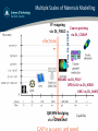
Multiple Scales of Materials Modelling
Coarse graining
MC via DL_MONTE
FF mapping
via DL_FIELD
via DL_CGMAP
MS&MD via DL_POLY
DPD & LB via DL_MESO
KMC via DL_AKMC
QM/MM bridging
via #ChemShell
STFC Daresbury Laboratory
Alice’s Wonderland (1865)
Lewis Carroll (Charles Lutwidge Dodgson)
Part 1
DL_POLY Project Background
DL_POLY Trivia
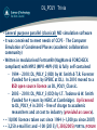
•  General purpose parallel (classical) MD simulation software
•  It was conceived to meet needs of CCP5 - The Computer
Simulation of Condensed Phases (academic collaboration
community)
•  Written in modularised Fortran90 (NagWare & FORCHECK
compliant) with MPI2 (MPI1+MPI-I/O) & fully self-contained
-  1994 – 2010: DL_POLY_2 (RD) by W. Smith & T.R. Forester
(funded for 6 years by EPSRC at DL). In 2010 moved to a
BSD open source licence as DL_POLY_Classic.
-  2003 – 2010: DL_POLY_3 (DD) by I.T. Todorov & W. Smith
(funded for 4 years by NERC at Cambridge). Up-licensed
to DL_POLY_4 in 2010 – free of charge to academic
researchers and at cost to industry (provided as source).
•  ~ 18,000 licences taken out since 1994 (~1,500 pa since 2007)
•  ~ 3,250 e-mail list and ~100 (2015)/1,350(2005) PORTAL/FORUM
Current Versions
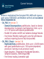
Written in modularised free formatted F90 (+MPI) with rigorous
code syntax (FORCHECK and NAGWare verified) and no external
library dependencies
•  DL_POLY_4 (version 7)
–  Domain Decomposition parallelisation, based on domain
decomposition (no dynamic load balancing), limits: up to
≈2.1×109 atoms with inherent parallelisation
–  Parallel I/O (amber netCDF) and radiation damage features
–  Free format (flexible) reading with some fail-safe features
and basic reporting (but not fully fool-proofed)
•  DL_POLY_Classic (version 1.9)
–  Replicated Data parallelisation, limits up to ≈30,000 atoms
with good parallelisation up to 100 (system dependent)
processors (running on any processor count)
–  Hyper-dynamics, Temperature Accelerated Dynamics,
Solvation Dynamics, (Path Integral MD)
–  Free format reading (somewhat rigid)
DL_POLY on the Web
WWW:
http://www.ccp5.ac.uk/DL_POLY/
FTP:
ftp://ftp.dl.ac.uk/ccp5/DL_POLY/
DEV:
http://ccpforge.cse.rl.ac.uk/gf/project/dl-poly/
http://ccpforge.cse.rl.ac.uk/gf/project/dl_poly_classic/
PORTAL: http://community.hartree.stfc.ac.uk/portal/site/
DL_SOFTWARE/
Further Information
W. Smith and T.R. Forester,
J. Molec. Graphics (1996), 14, 136
W. Smith, C.W. Yong, P.M. Rodger,
Molecular Simulation (2002), 28, 385
I.T. Todorov, W. Smith, K. Trachenko, M.T. Dove,
J. Mater. Chem. (2006), 16, 1611-1618
W. Smith (Guest Editor),
Molecular Simulation (2006), 32, 933
I.J. Bush, I.T. Todorov and W. Smith,
Comp. Phys. Commun. (2006), 175, 323-329
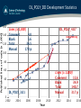
DL_POLY_DD Development Statistics
Published lines of code [x 1,000]
160
140
120
100
80
60
40
20
Lines [x 1,000]
Comment
4.0
Blank 5.6
Total 36.5
Manual
178 p
ered
e
n
i
g
reen
DL_POLY_3.01
0
2002
2004
2006
DL_POLY_4.07
reengineering Lines [x 1,000]
Comment
15.6
Blank 34.9
Total 140.7
Manual
317 p
2008
Year
2010
2012
2014
2016
2000
1500
1000
500
0
1992
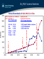
2014 Usage Statistics
• 540 Google Scholar citations
• 1,120 downloads
• 3,050 eMail list
1996
2000
2004
Year
DL_POLY_C
2500
2014 Downloads
• EU-UK– 20.1%
• UK
– 18.5%
• USA – 11.9%
• China – 11.6%
• India – 7.0%
• France- 4.4%
web-registration 3000
DL_POLY_4
2010 :: DL_POLY (2+3+MULTI) - 1,000 (list end)
2013 :: DL_POLY_4
- 3,250 (list start 2011)
DL_POLY_3
3500
Annual Downloads & Valid eMail List Size
DL_POLY_2
Count
DL_POLY Licence Statistics
2008
2012
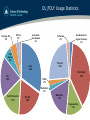
DL_POLY Usage Statistics
Europe-EU
5%
Australia & New Zealand 2% Africa
2%
Software
2%
La#n America 8% Bio-­‐Molecular & Organic Chemsitry 4% Physics
24%
Asia
32%
Chemistry
37%
UK
19%
Other
2%
Mechanics
2%
North America
15%
EU-UK
20%
Materials
17%
Engineering
13%
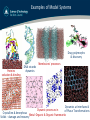
Examples of Model Systems
Drug polymorphs
& discovery
Proteins
solvation & binding
DNA strands
dynamics
Membranes processes
Dynamics at Interfaces &
Dynamic processes in
of Phase Transformations
Crystalline & Amorphous Metal-Organic & Organic Frameworks
Solids – damage and recovery
Part 2
The Molecular Dynamics Method
Molecular Dynamics: Definitions
•  Theoretical tool for modelling the detailed microscopic behaviour
of many different types of systems, including; gases, liquids,
solids, polymers, surfaces and clusters.
•  In an MD simulation, the classical equations of motion governing
the microscopic time evolution of a many body system are solved
numerically, subject to the boundary conditions appropriate for
the geometry or symmetry of the system.
•  Can be used to monitor the microscopic mechanisms of energy
and mass transfer in chemical processes, and dynamical
properties such as absorption spectra, rate constants and
transport properties can be calculated.
•  Can be employed as a means of sampling from a statistical
mechanical ensemble and determining equilibrium properties.
These properties include average thermodynamic quantities
(pressure, volume, temperature, etc.), structure, and free energies
along reaction paths.
Molecular Dynamics for Beginners
MD simulations are used for:
•  Microscopic insight: we can follow the
motion of a single molecule (glass of
water)
•  Investigation of phase change (NaCl)
•  Understanding of complex systems like
polymers (plastics – hydrophilic and
hydrophobic behaviour)
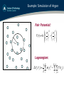
Example: Simulation of Argon
Pair Potential:
rcut
!
⎧⎪⎛ σ ⎞12 ⎛ σ ⎞6 ⎫⎪
V (r ) = 4ε ⎨⎜ ⎟ − ⎜ ⎟ ⎬
⎪⎩⎝ r ⎠ ⎝ r ⎠ ⎪⎭
Lagrangian:
N −1
1N
! !
L(ri , vi ) = ∑ mi vi 2 − ∑ ∑ V (rij )
2 i
i j >i
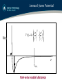
Lennard -Jones Potential
⎧⎪⎛ σ ⎞12 ⎛ σ ⎞6 ⎫⎪
V (r ) = 4ε ⎨⎜ ⎟ − ⎜ ⎟ ⎬
⎪⎩⎝ r ⎠ ⎝ r ⎠ ⎪⎭
V(r)
σ
r
ε
rcut!
Pair-wise radial distance
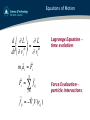
Equations of Motion
d ⎛ ∂ L ⎞ ∂ L
⎜ α ⎟ = α
dt ⎝ ∂ vi ⎠ ∂ ri
!
!
mi ai = Fi
N !
!
Fi = ∑ f ij
j ≠i
!
!
f ij = −∇ iV (rij )
Lagrange Equation –
time evolution
Force Evaluation –
particle interactions
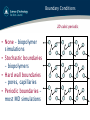
Boundary Conditions
2D cubic periodic
•  None – biopolymer
simulations
•  Stochastic boundaries
– biopolymers
•  Hard wall boundaries
– pores, capillaries
•  Periodic boundaries –
most MD simulations
Periodic Boundary Conditions
Triclinic
Truncated octahedron
Hexagonal prism
Rhombic dodecahedron
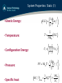
System Properties: Static (1)
1 N
2
K.E. =
m
v
∑ ii
2 i
•  Kinetic Energy:
2
T=
K.E.
3NkB
•  Temperature:
N
Uc =
•  Configuration Energy:
•  Pressure:
•  Specific heat:
∑∑V (r )
ij
i
1
PV = NkBT −
3
δ (Uc )
2
NVE
j>i
! !
∑ ri ⋅ fi
N
i
3 2 2 " 3NkB %
= NkBT $1−
'
2
2Cv &
#
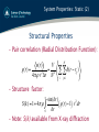
System Properties: Static (2)
Structural Properties
–  Pair correlation (Radial Distribution Function):
n(r)
V
g(r) =
= 2
2
4π ρ r Δr N
N
∑∑δ (r − r )
ij
i
j≠i
–  Structure factor:
∞
S(k) = 1+ 4π ρ ∫
0
sin(kr)
2
g(r)
−1
r
(
) dr
kr
–  Note: S(k) available from X-ray diffraction
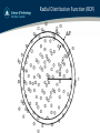
Radial Distribution Function (RDF)
ΔR
R
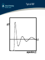
Typical RDF
g(r)!
1.0!
separation (r)!
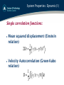
System Properties: Dynamic (1)
Single correlation functions:
l 
Mean squared displacement (Einstein
relation)
1
2
2Dt = | ri (t) − ri (0) |
3
l 
Velocity Autocorrelation (Green-Kubo
relation)
1
D = ∫ vi (t)⋅ vi (0) dt
3
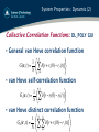
System Properties: Dynamic (2)
Collective Correlation Functions: DL_POLY GUI
•  General van Hove correlation function
1
G (r, t ) =
N
N
∑ δ [r + r (0) − r (t )]
i
j
i , j =1
•  van Hove self-correlation function
1
Gs (r, t ) =
N
N
∑δ [r − r (0) − r (t )]
i
i
i
•  van Hove distinct correlation function
1
Gd (r, t ) =
N
N
N
∑∑ δ [r + r (0) − r (t )]
i
i
j ≠i
j
Correlation Function Uses
•  Complete description of bulk dynamical
properties
•  Space-time Fourier Transform of van Hove
function
•  Elastic properties of materials
•  Energy dissipation
•  Sound propagation
Obtained directly from neutron scattering
Part 3
DL_POLY Basics & Algorithms
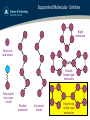
Supported Molecular Entities
Rigid
molecules
Point ions
and atoms
Flexibly
linked rigid
molecules
Polarisable
ions (core
+shell)
Flexible
molecules
Constraint
bonds
Rigid bond
linked rigid
molecules
Force Field Definitions – I
•  particle: a rigid ion or an atom (charged or not), a core or a shell
of a polarisable ion (with or without associated degrees of
freedom), a massless charged site. A particle is a countable
object and has a global ID index.
•  site: a particle prototype that serves to define the chemical &
physical nature (topology/connectivity/stoichiometry) of a
particle (mass, charge, frozen-ness). Sites are not atoms they are
prototypes!
•  Intra-molecular interactions: chemical bonds, bond angles,
dihedral angles, improper dihedral angles, inversions. Usually,
the members in a unit do not interact via an inter-molecular term.
However, this can be overridden for some interactions. These are
defined by site.
•  Inter-molecular interactions: van der Waals, metal (2B/E/EAM,
Gupta, Finnis-Sinclair, Sutton-Chen), Tersoff, three-body, fourbody. Defined by species.
Force Field Definitions – II
•  Electrostatics: Standard Ewald*, Hautman-Klein (2D) Ewald*,
SPM Ewald (3D FFTs), Force-Shifted Coulomb, Reaction Field,
Fennell damped FSC+RF, Distance dependent dielectric constant,
Fuchs correction for non charge neutral MD cells.
•  Ion polarisation via Dynamic (Adiabatic) or Relaxed shell model.
•  External fields: Electric, Magnetic, Gravitational, Oscillating &
Continuous Shear, Containing Sphere, Repulsive Wall.
•  Intra-molecular like interactions: tethers, core shells units,
constraint and PMF units, rigid body units. These are also
defined by site.
•  Potentials: parameterised analytical forms defining the
interactions. These are always spherically symmetric!
•  THE CHEMICAL NATURE OF PARTICLES DOES NOT CHANGE
IN SPACE AND TIME!!! *
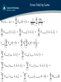
Force Field by Sums
!!
!
V( r1, r2 ,....., rN ) =
N'
∑
! !
U pair (| ri − rj |) +
i,j
N'
∑U
Tersoff
(
! ! !
ri , rj, rk ) +
i,j,k
N'
∑U
N bond
U bond (
! !
i bond , ra , rb ) +
N
N'
∑
U 4−body (
! ! ! !
ri , rj, rk , rn ) +
∑
i
% N'
! ! ((
F '' ∑ ρij (| ri − rj |)**** +
& i,j
))
N angle
! ! !
U angle ( iangle , ra , rb , rc ) +
∑
U dihed (
! ! ! !
idihed , ra , rb , rc , rd ) +
idihed
N invers
∑
! ! ! !
U invers ( i invers , ra , rb , rc , rd ) +
iinvers
N tether
itether
i,j
iangle
N dihed
∑
∑
q iq j
! ! +
| ri − rj |
i,j,k,n
ibond
∑
(
N'
! ! !
ri , rj, rk ) +
i,j,k
% N'
! !
'
εmetal ' ∑ Vpair (| ri − rj |) +
& i,j
∑
3−body
1
4πεε 0
U tether (
! !
i tether , rt , rt=0 ) +
N core-shell
∑
icore-shell
U core-shell (
! !
icore-shell , | ri − rj |) +
N
∑
i=1
!
Φexternal ( ri )
Boundary Conditions
•  None (e.g. isolated macromolecules)
•  Cubic periodic boundaries
•  Orthorhombic periodic boundaries
•  Parallelepiped (triclinic) periodic boundaries
•  Truncated octahedral periodic boundaries*
•  Rhombic dodecahedral periodic boundaries*
•  Slabs (i.e. x,y periodic, z non-periodic)
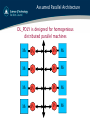
Assumed Parallel Architecture
DL_POLY is designed for homogenious
distributed parallel machines
M0
P0
P4
M4
M1
P1
P5
M5
M2
P2
P6
M6
M3
P3
P7
M7
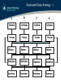
Replicated Data Strategy – I
A
B
Initialize!
Initialize!
Initialize!
Initialize!
Forces!
Forces!
Forces!
Forces!
C
D
Motion!
Motion!
Motion!
Motion!
Statistics!
Statistics!
Statistics!
Statistics!
Summary!
Summary!
Summary!
Summary!
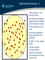
Replicated Data Strategy – II
•  Every processor sees
the full system
•  No memory distribution
(performance overheads
and limitations increase
with increasing system
size)
•  Functional/algorithmic
decomposition of the
workload
•  Cutoff ≤ 0.5 min system
width
•  Extensive global
communications
(extensive overheads
increase with increasing
system size)
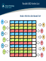
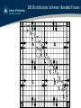
Parallel (RD) Verlet List
Brode-Ahlrichs distributed list!
A!
C!
A!
C!
A!
C!
1,2
1,3
1,4
1,5
1,6
1,7
2,3
2,4
2,5
2,6
2,7
2,8
3,4
3,5
3,6
3,7
3,8
3,9
4,5
4,6
4,7
4,8
4,9
4,10
5,6
5,7
5,8
5,9
5,10
5,11
6,7
6,8
6,9
6,10
6,11
6,12
7,8
7,9
7,10
7,11
7,12
8,9
8,10
8,11
8,12
8,1
9,10
9,11
9,12
9,1
9,2
10,11
10,12
10,1
10,2
10,3
11,12
11,1
11,2
11,3
11,4
12,1
12,2
12,3
12,4
12,5
B!
D!
B!
D!
B!
D!
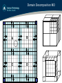
Domain Decomposition MD
A!
B!
C!
D!
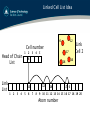
Linked Cell Lists
•  Linked lists provide an elegant way to scale short-ranged
two body interactions from O(N2/2) to ≈O(N). The efficiency
increases with increasing link cell partitioning – as a rule of
thumb best efficacy is achieved for cubic-like partitioning
with number of link-cells per domain ≥ 4 for any dimension.
•  Linked lists can be used with the same efficiency for 3-body
(bond-angles) and 4-body (dihedral & improper dihedral &
inversion angles) interactions. For these, the linked cell
halo is double-layered and as cutoff3/4-body ≤ 0.5*cutoff2-body
this makes the partitioning more effective than that for the
2-body interactions.
•  The larger the particle density and/or the smaller the cutoff
with respect to the domain width, (the larger the sub-selling
and the better the spherical approximation of the search
area), the shorter the Verlet neighbour-list search.
Linked Cell List Idea
6
Cell number
Head of Chain
List
Link
List 17
1 2 3 4 5
6
10
12
16
12
16
Link
Cell 2
10
17 0
1 2 3 4 5 6 7 8 9 10 11 12 13 14 15 16 17 18 19 20
Atom number
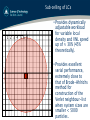
Sub-celling of LCs
1 2 3 4 5 6 7
•  Provides dynamically
adjustable workload
for variable local
density and VNL speed
up of ≈ 30% (45%
theoretically).
•  Provides excellent
serial performance,
extremely close to
that of Brode-Ahlrichs
method for
construction of the
Verlet neighbour-list
when system sizes are
smaller < 5000
particles.
Conditional Update of the VNL
•  Replicated Data Shell Stripping – the VNL build up is extended
for rcut+δr (shell width). The extended two body list is rebuild
only and only when a pair of neighbouring particles has
travelled more than δr apart since the last VNL build point.
Rule of thumb δr/rcut≈5-15%. •  Domian Decomposition Particle Blurring – the VNL build up is
extended for rcut+δr (domain padding). The extended two
body list is rebuild only and only when a particle has travelled
apart more than δr/2 apart since the last VNL build point.
Rule of thumb δr/rcut≈1-5%.
•  Consequences:
•  All short-ranged force evaluations have an additional
check on pairs distance!
•  Memory and Communication over Computation and
Communication balance. Force field (FF) dependent.
•  Short ranged FF 60-100% gains, FF with Ewald 10-35%.
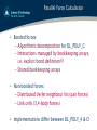
Parallel Force Calculation
•  Bonded forces:
-  Algorithmic decomposition for DL_POLY_C
-  Interactions managed by bookkeeping arrays,
i.e. explicit bond definition!!!
-  Shared bookkeeping arrays
•  Non-bonded forces:
-  Distributed Verlet neighbour list (pair forces)
-  Link cells (3,4-body forces)
•  Implementations differ between DL_POLY_4 & C!
P0Local
force
terms
P1Local
force
terms
P2Local
force
terms
Processors
Molecular
force field
definition
Global Force Field
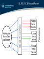
DL_POLY_C & Bonded Forces
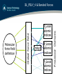
P0Local
atomic
indices
Tricky!
P1Local
atomic
indices
P2Local
atomic
indices
Processor Domains
Molecular
force field
definition
Global force field
DL_POLY_4 & Bonded Forces
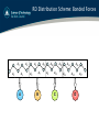
RD Distribution Scheme: Bonded Forces
A2
A1
A6
A4
A3
A!
A5
A10
A8
A7
B!
A9
A11
C!
A16
A14
A12
A13
A17
A15
D!
DD Distribution Scheme: Bonded Forces
A!
B!
C!
D!
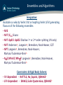
Ensembles and Algorithms
Integration:
Available as velocity Verlet (VV) or leapfrog Verlet (LFV) generating
flavours of the following ensembles
•  NVE
•  NVT (Ekin) Evans
•  NVT dpdS1 dpdS2 Sharlow 1st or 2nd order splitting (VV only)
•  NVT Andersen^, Langevin^, Berendsen, Nosé-Hoover, GST
•  NPT Langevin^, Berendsen, Nosé-Hoover,
Martyna-Tuckerman-Klein^
•  NσT/NPnAT/NPnγT Langevin^, Berendsen, Nosé-Hoover,
Martyna-Tuckerman-Klein^
Constraints & Rigid Body Solvers:
•  VV dependent – RATTLE, No_Squish, QSHAKE*
•  LFV dependent – SHAKE, Euler-Quaternion, QSHAKE*
Integration Algorithms
Essential Requirements:
• 
• 
• 
• 
• 
• 
Computational speed
Low memory demand
Accuracy
Stability (energy conservation, no drift)
Useful property - time reversibility
Extremely useful property – symplecticness
= time reversibility + long term stability
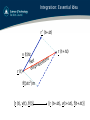
Integration: Essential Idea
r’ (t+Δt)
v (t)Δt
r (t)
r (t+Δt)
t
n
t
e
Ne lacem
disp
f(t)Δt2/m
[r (t), v(t), f(t)]
[r (t+Δt), v(t+Δt), f(t+Δt)]
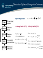
Simulation Cycle and Integration Schemes
Taylor expansion:
Setup
Set up initial
system
Forces
Calculate
forces
Motion
Calculate
motion
Stats.
Results
Accumulate
statistical data
Summarise
simulation
Δt 2 f n
rn+1 = rn + Δt vn +
+ O Δt 3
2 m
( )
Leapfrog Verlet (LFV)
Velocity Verlet (VV)
0. x i (t ), vi (t − 12 Δt )
VV1.0. x i (t ), vi (t ), f i (t )
1. f i (t ) − calculated afresh
VV1.1. vi (t + 12 Δt ) = vi (t ) +
Δt f i (t )
2 mi
f i (t )
mi VV1.2. x (t + Δt ) = xi (t ) + Δt v (t + 1 Δt )
i
i
2
2
3. xi (t + Δt ) = xi (t ) + Δt vi (t + 12 Δt )
VV2.0. f i (t + Δt ) − calculated afresh
2. vi (t + 12 Δt ) = vi (t − 12 Δt ) + Δt
VV2.1. vi (t + Δt ) = vi (t + 12 Δt ) +
Δt f i (t + Δt )
2
mi
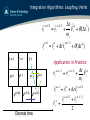
Integration Algorithms: Leapfrog Verlet
! n +1/ 2 ! n −1/ 2 Δt ! n
vi
= vi
+ Fi + ϑ (Δt 3 )
mi
! n +1 ! n
! n +1/ 2
ri = ri + Δtvi
+ ϑ (Δt 4 )
f n-2"
rn-2"
f n-1"
rn-1"
f n"
rn "
Application in Practice
rn+1"
vn-3/2" vn-1/2" vn+1/2"
Discrete time"
! n +1/ 2 ! n −1/ 2 Δt ! n
vi
= vi
+
Fi
mi
! n +1 ! n
! n +1/ 2
ri = ri + Δtvi
! n +1/ 2 ! n −1/ 2
! n vi
+ vi
vi =
2
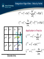
Integration Algorithms: Velocity Verlet
! n +1 ! n
! n Δt 2 ! n
ri = ri + Δtvi +
Fi + ϑ (Δt 4 )
2mi
! n +1 ! n Δt ! n ! n +1
vi = vi +
( Fi + Fi ) + ϑ (Δt 2 )
2mi
f n-2"
f n-1"
f n"
f n+1"
rn-2"
rn-1"
rn "
rn+1"
vn-2"
vn-1"
vn"
vn+1"
Discrete time"
Application in Practice
! n +1/ 2 ! n
Δt ! n
vi
= vi +
Fi
2mi
! n +1 ! n
! n +1/ 2
ri = ri + Δtvi
! n +1 ! n +1/ 2
Δt ! n +1
vi = vi
+
Fi
2mi
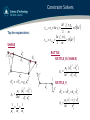
Constraint Solvers
Δt 2 f n + g n
rn +1 = rn + Δt vn +
+ O Δt 3
2
m
Δt f n + hn
vn +1 = vn + 1 +
+ O(Δt 3 )
2
2 m
( )
Taylor expansions:
SHAKE
iu
!
Gij i
io
!u
!d ij
d ij
j
!o
o
d ij
j
!o
!
!
Gij = − G ji ≈ g ij d ij
! 2 !u2
µij (d ij − d ij )
!o !u
g ij =
2
2Δt
d ij ⋅ d ij
1
µij
=
1
1
+
mi m j
RATTLE
RATTLE_R (SHAKE)
!
G ji
!o2 !u 2
µij (d ij − d ij )
g ij = 2 ! o ! u
Δt
d ij ⋅ d ij
ju
!
vio
i
j
!
d ij
RATTLE_V
!
vio
!o
!
!
H ij = − H ji = hij ⋅ d ij
! ! !o
µij (vi − v j ) ⋅ d ij
hij =
Δt
d ij2
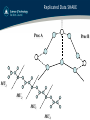
Replicated Data SHAKE
Proc A
Proc B
MU1
MU2
MU3
MU4
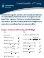
Extended Ensembles in VV casting
Velocity Verlet integration algorithms can be naturally derived from the
non-commutable Liouvile evolution operator by using a second order
Suzuki-Trotter expansion. Thus they are symplectic/true ensembles
(with conserved quantities) warranting conservation of the phase-space
volume, time-reversibility and long term numerical stability…
Examplary VV Expansion of NVE to NVEkin, NVT, NPT & NσT
VV2 :
VV1 :
x i (t ), vi (t ), f i (t )
x i (t + Δt ), vi (t + 12 Δt ), f i (t + Δt ) − afresh
Thermostat (t → t + 14 Δt )
: 14 Δt
Barostat (t → t + 12 Δt )
: 12 Δt
vi (t + Δt ) = vi (t + 12 Δt ) +
Δt f i (t + Δt ) 1
: 2 Δt
2
mi
Thermostat (t + 14 Δt → t + 12 Δt ) : 14 Δt
RATTLE _ V (t + 12 Δt → t + Δt )
: Δt
Δt f i (t )
vi (t + Δt ) = vi (t ) +
2 mi
Thermostat (t + 12 Δt → t + 34 Δt )
: 14 Δt
Barostat (t + 12 Δt → t + Δt )
: 12 Δt
Thermostat (t + 32 Δt → t + Δt )
: 14 Δt
1
2
: Δt
1
2
Δt
xi (t + Δt ) = xi (t ) +
vi (t + 12 Δt ) : Δt
2
RATTLE _ R(t → t + Δt )
: Δt
Dissipative Particle Dynamics
•  Similar methodology to classical MD:
–  Condensed phase system modelled by particles
(‘beads’) using pairwise potentials
–  Particle motion determined by force integration (e.g.
Velocity Verlet)
–  System properties at equilibrium calculated as ensemble
averages
•  System coupled to heat bath using pairwise
dissipative and random forces
–  Pairwise thermostatting conserves system momentum
and produces correct hydrodynamics
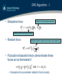
DPD Algorithm - I
•  Dissipative force:
Relative velocity between particles
!!"! = −!! ! !!" !!" ⋅ !!" !!" !
Distance-based screening function
•  Random force:
Gaussian random number (zero mean, unity variance)
!!"!
=
!! !
!!"
!!"
!"
!!" !
•  Fluctuation-dissipation theory demonstrates these
forces act as thermostat if:
!
!
!!" = !
!
!!"
!
and !! ! = 2!! !"!
–  Dissipative force parameter related to fluid viscosity
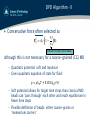
DPD Algorithm - II
•  Conservative force often selected as
!!"!
= !!"
!!"
1−
! !
!! !"
Interaction length (cutoff radius)
although this is not necessary for a coarse-grained (CG) MD –  Quadratic potential: soft and repulsive
–  Gives quadratic equation of state for fluid:
! ≈ !!! ! + 0.101!!" !! !!! !
–  Soft potential allows for larger time steps than classical MD:
beads can ‘pass through’ each other and reach equilibrium in
fewer time steps
–  Flexible definition of beads: either coarse-grains or
‘momentum carriers’
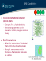
DPD Capabilities
•  Flexible interactions between
species pairs Hydrophilic head
Hydrophobic tail
–  Can specify e.g. hydrophobicity
–  Interaction parameters can be
connected to Flory-Huggins solution
theory
•  Bond interactions
–  Allow for construction of ‘molecules’
from differently interacting beads
–  Example: spontaneous vesicle
formation of amphiphilic molecules
in solution
Source: Yamamoto et al., J Chem Phys,
116, 5842–5849 (2002)
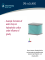
DPD via DL_MESO
–  Example: formation of
water drops on
hydrophobic surface
under influence of
gravity
Source: Johansson, Simulating fluid flow
and heat transfer using dissipative particle
Dynamics, Dept. Energy Sci., Lund
University (2012)
Other Integration Algorithms
• Gear Predictor-Corrector – generally easily
extendable to any high order of accuracy. It
is used in satellite trajectory calculations/
corrections. However, lacking long term
stability.
• Trotter derived evolution algorithms –
generally easily extendable to any high
order of accuracy. Symplectic.
Base Functionality
•  Molecular dynamics of polyatomic systems with
options to save the micro evolution trajectory at
regular intervals
•  Optimisation by conjugate gradients method or zero
Kelvin annealing
•  Statistics of common thermodynamic properties
(temperature, pressure, energy, enthalpy, volume)
with options to specify collection intervals and stack
size for production of rolling and final averages
•  Calculation of RDFs and Z-density profiles
•  Temperature scaling, velocity re-Gaussing
•  Force capping in equilibration
DL_POLY_4 Specials
•  Radiation damage driven features:
-  defects analysis
-  boundary thermostats
-  volumetric expansion
-  replay history
-  variable time step algorithm
•  Extra ensembles:
-  DPD, Langevin, Andersen, MTK, GST
-  extensions of NsT to NPnAT and NPnγT
•  Infrequent k-space Ewald evaluation
•  Direct VdW
•  Direct Metal
•  Force shifted VdW
•  I/O driven features Parallel I/O & netCDF
•  Extra Reporting
Part 4
DL_POLY I/O Files
I/O Files
REVCON
CONFIG
CFGMIN*
REFERENCE*
OUTPUT
STATIS
TABBND*
I/O FILES
FIELD
TABEAM*
•  Restart data
DEFECTS*
CONTROL
TABLE*
•  Tabulated
interactions
HISTORY*, HISTORF*
HISTORY*
DL_POLY_4
•  Crystallographic
(Dynamic) data
•  Reference data for
DEFECTS
•  Traj. data for replay
•  Simulation controls
•  Molecular/
Topological Data
MSDTMP*, RSDDAT*
VAFDAT_*
•  Final & CGM
configurations
•  Best CGM configuration
•  Simulation summary
data
•  Trajectory data
•  Defects data
•  Statistics data
•  RSD, MSD & T inst data
•  VAF data
BNDDAT*, BNDPMF*, BNDTAB*
ANGDAT*, ANGPMF*, ANGTAB*
TABANG*
DIHDAT*, DIHPMF*, DIHTAB*
TABDIH*
INVDAT*, INVPMF*, INVTAB*
TABINV*
RDFDAT*, VDWPMF*, VDWTAB*
REVOLD*
ZDNDAT*
REVIVE
•  Intra PDF data
•  Inter PDF/RDF data
•  Z density data
•  Restart data
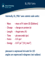
DL_POLY Units
Internally, DL_POLY uses atomic scale units:
• 
• 
• 
• 
• 
• 
Mass
Charge
Length
Time
Force
Energy
–
–
–
–
–
–
mass of H atom (D) [Daltons]
charge on proton (e)
Angstroms (Å)
picoseconds (ps)
D Å ps-2
D Å2 ps-2 [10 J mol-1]
pressure is expressed in k-atm for I/O
angles are expressed in degrees (not radians)
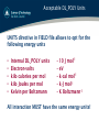
Acceptable DL_POLY Units
UNITS directive in FIELD file allows to opt for the
following energy units
• 
• 
• 
• 
• 
Internal DL_POLY units
Electron-volts
kilo calories per mol
kilo Joules per mol
Kelvin per Boltzmann
–
–
–
–
–
10 J mol-1
eV
k-cal mol-1
k-J mol-1
K Boltzmann-1
All interaction MUST have the same energy units!
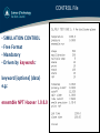
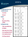
CONTROL File
•  SIMULATION CONTROL
•  Free Format
•  Mandatory
•  Driven by keywords:
keyword [options] {data}
e.g.:
ensemble NPT Hoover 1.0 8.0
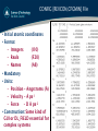
CONFIG [REVCON,CFGMIN] File
• Initial atomic coordinates
• Format
-  Integers
(I10)
-  Reals
(F20)
-  Names
(A8)
• Mandatory
• Units:
-  Position – Angstroms (Å)
-  Velocity – Å ps-1
-  Force
– D Å ps-2
• Construction: Some kind of
GUI or DL_FIELD essential for
complex systems
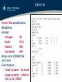
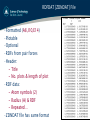
FIELD File
• Force Field specification
• Mandatory
• Format:
-  Integers
(I5)
-  Reals
(F12)
-  Names
(A8)
-  Keywords
(A4)
• Maps on to CONFIG file
structure
• Construction
-  Small systems – by hand
-  Large systems – nfold or
GUI or DL_FIELD!
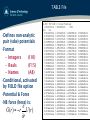
TABLE File
• Defines non-analytic
pair (vdw) potentials
• Format
-  Integers
(I10)
-  Reals
(F15)
-  Names
(A8)
• Conditional, activated
by FIELD file option
• Potential & Force
• NB force (here) is:
∂
G (r ) = −r U (r )
∂r
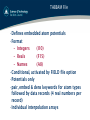
TABEAM File
• Defines embedded atom potentials
• Format
-  Integers
(I10)
-  Reals
(F15)
-  Names
(A8)
• Conditional, activated by FIELD file option
• Potentials only
• pair, embed & dens keywords for atom types
followed by data records (4 real numbers per
record)
• Individual interpolation arrays
REVOLD [REVIVE] File
• Provides program restart capability
• File is unformatted (not human readable)
• Contains thermodynamic accumulators, RDF data,
MSD data and other checkpoint data
• REVIVE (output file) ---> REVOLD (input file)
OUTPUT File
• Provides Job Summary (mandatory!)
• Formatted to be human readable
• Contents:
-  Summary of input data
-  Instantaneous thermodynamic data at selected intervals
-  Rolling averages of thermodynamic data
- 
- 
- 
- 
Statistical averages
Final configuration
Radial distribution data
Estimated mean-square displacements and 3D diffusion
coefficient
• Plus:
-  Timing data, CFG and relaxed shell model iteration data
-  Warning & Error reports
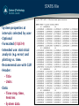
STATIS File
• System properties at
intervals selected by user
• Optional
• Formatted (I10,E14)
• Intended use: statistical
analysis (e.g. error) and
plotting vs. time.
• Recommend use with GUI!
• Header:
-  Title
-  Units
• Data:
-  Time step, time,
#entries
-  System data
HISTORY File
•  Configuration data at user
selected intervals
-  Formatted
-  Optional
•  Header:
-  Title
-  Data level, cell key,
number
•  Configuration data:
-  Time step and data keys
-  Cell Matrix
-  Atom name, mass, charge
-  X,Y,Z coordinates (level 0)
-  X,Y,Z velocities (level 1)
-  X,Y,Z forces (level 2)
RDFDAT [ZDNDAT] File
• Formatted (A8,I10,E14)
• Plotable
• Optional
• RDFs from pair forces
• Header:
-  Title
-  No. plots & length of plot
• RDF data:
-  Atom symbols (2)
-  Radius (A) & RDF
-  Repeated…
• ZDNDAT file has same format
DL_POLY_4 Extra Files
• REFERENCE file
- Reference structure to compare against
• DEFECTS file
- Trajectory file of vacancies and interstitials migration
• MSDTMP file
- Trajectory like file containing particles’ Sqrt(MSDmean) and Tmean
• RSDDAT file
- Trajectory like file containing particles’ Sqrt(RSD from origin)
• TABINT file
- Table file for INTra-molecular interactions
• INTDAT file
- Probability Distribution Functions for INTra-molecular interactions
• HISTORF file
- Force replayed HISTORY
• …
Part 5
DL_POLY_4 Performance
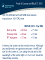
Proof of Concept on IBM p575 2005
300,763,000 NaCl with full SPME electrostatics
evaluation on 1024 CPU cores
Start-up time
Timestep time
FFT evaluation
HECToR (2013 – Cray XE6)
≈ 60 min
≈ 15 min
≈ 68 sec
≈ 23 sec
≈ 55 sec
≈ 18 sec
In theory ,the system can be seen by the eye. Although
you would need a very good microscope – the MD cell
size for this system is 2μm along the side and as the
wavelength of the visible light is 0.5μm so it should be
theoretically possible.
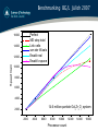
Benchmarking BG/L Jülich 2007
Perfect
MD step total
Link cells
van der Waals
Ewald real
Ewald k-space
16000
14000
Speed Gain
12000
10000
8000
6000
4000
14.6 million particle Gd2Zr2O7 system
2000
2000
4000
6000
8000
10000
Processor count
12000
14000
16000
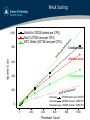
Weak Scaling
Solid Ar (32'000 atoms per CPU)
NaCl (27'000 ions per CPU)
SPC Water (20'736 ions per CPU)
1000
800
Speed Gain
fec
r
pe
on
i
t
a
lis
e
l
l
33 million atoms
ra
a
p
t
28 million atoms
600
400
21 million atoms
llelisation
a
r
a
p
d
o
go
200
max load
max load
max load
0
0
200
400
600
Processor Count
700'000 atoms per 1GB/CPU
220'000 ions per 1GB/CPU
210'000 ions per 1GB/CPU
800
1000
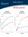
DL_POLY_4 RB v/s CB
HECToR (Cray XE6) 2013
Weak Scaling and Cost of Complexity
HECToR (Cray XE6) 2013
1.8
1.6
Time per timestep [s]
1.4
1.2
1
0.8
Argon
Transferrin
NaCl
RB water
CB water
0.6
0.4
0.2
0
0 200 400 600 MPI tasks count
800 1000 I/O Solutions
1.  Serial read and write (sorted/unsorted) – where only a single
MPI task, the master, handles it all and all the rest communicate
in turn to or get broadcasted to while the master completes
writing a configuration of the time evolution.
2.  Parallel write via direct access or MPI-I/O (sorted/unsorted)
– where ALL / SOME MPI tasks print in the same file in some
orderly manner so (no overlapping occurs using Fortran direct
access printing. However, it should be noted that the behaviour
of this method is not defined by the Fortran standard, and in
particular we have experienced problems when disk cache is not
coherent with the memory).
3.  Parallel read via MPI-I/O or Fortran
4.  Serial NetCDF read and write using NetCDF libraries for
machine-independent data formats of array-based, scientific
data (widely used by various scientific communities).
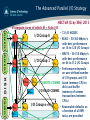
The Advanced Parallel I/O Strategy
HECToR (Cray XE6) 2013
P0
P1
M0
M1
I/O BATCH
I/O Group 0
•  72 I/O NODES
PX0-1
MX1-1
PX0
PX0+1
MX0
MX0+1
DISK
I/O BATCH I/O BATCH
N compute cores of which M < N do I/O
PHEAD
I/O Group 1
PXn+1
MXn
MXn+1
•  WRITE ~ 50-150 Mbyte/s
with best performance
on 64 to 512 I/O Groups
•  Performance depends
on user defined number
of I/O groups, and I/O
I/O WRITE COMMS batch (memory CPU to
disk) and buffer
I/O READ COMMS (memory of comms
transactions between
CPUs)
MX1-1
Pslave
Memory
PXn
PX1-1
•  READ ~ 50-300 Mbyte/s
with best performance
on 16 to 128 I/O Groups
I/O Group n=M-1
PN-1
MN-1
•  Reasonable defaults as
a function of all MPI
tasks are provided
Part 5
Obtaining & Building DL_POLY
DL_POLY Licensing and Support
•  Online Licence Facility at http://www.ccp5.ac.uk/DL_POLY/
•  The licence is
-  To protect copyright of Daresbury Laboratory
-  To reserve commercial rights
-  To provide documentary evidence justifying continued
support by UK Research Councils
•  It covers only the DL_POLY_4 package
•  Registered users are entered on the DL_POLY e-mailing list
-  Support is available (under CCP5 & MCC SLA via EPSRC)
only to UK academic researchers
-  For the rest of the world there is the PORTAL
•  Last but not least there is a detailed, interactive, selfreferencing PDF (LaTeX) user manual
Supply of DL_POLY_4
• Register at http://www.ccp5.ac.uk/DL_POLY/
• Registration provides the decryption - procedure
and password (sent by e-mail)
• Source is supplied by anonymous FTP
• Source is in an encrypted zip file
• Successful unpacking produces a unix directory
structure
• Test and benchmarking data are also available on
the FTP
DL_POLY_Classic Support
•  Full documentation of software supplied with source
•  Support is available through the DL_SODFTWARE portal
or the CCP5 user community
WWW:
http://www.ccp5.ac.uk/DL_POLY_CLASSIC/
FTP:
ftp://ftp.dl.ac.uk/ccp5/DL_POLY/
PORTAL: http://community.hartree.stfc.ac.uk/portal/site/
DL_SOFTWARE/
Supply of DL_POLY_Classic
•  Downloads are available from CCPForge at
http://ccpforge.cse.rl.ac.uk/gf/project/dl_poly_classic/
•  No registration required – BSD licence
•  Download source from: CCPForge: Projects: DL_POLY
Classic: Files: dl_poly_classic: dl_poly_classic1.9
•  Sources is a in tarred and gzipped form
•  Successful unpacking produces a unix directory structure
•  Test data are also available
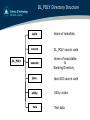
DL_POLY Directory Structure
build
source
DL_POLY
execute
Home of makefiles
DL_POLY source code
Home of executable
&
Working Directory
java
Java GUI source code
utility
Utility codes
data
Test data
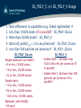
DL_POLY_C v/s DL_POLY_4 Usage
1.  Note differences in capabilities (e.g. linked rigid bodies) !!!
2.  Less than 10,000 atoms (if in parallel)? – DL_POLY Classic
3.  More than 30,000 atoms? – DL_POLY_4
4.  Ratio cell_width/rcut < 3 (in any direction)? – DL_POLY_Classic
5.  Less than 500 particles per processor? – DL_POLY_Classic
DL_POLY_Classic
Simple molecules (no SHAKE):
•  8 or less, 10,000 atoms
•  16 or less, 20,000 atoms
•  32 or less, 30,000 atoms
Simple ionics:
•  16 or less, 10,000 atoms
•  64 or less, 20,000 atoms
•  128 or less, 30,000 atoms
Molecules (with SHAKE):
•  64 max!
DL_POLY_4
•  Golden Rule 1: No fewer than
3x3x3 link cells per processor (if
in parallel)
•  Golden Rule 2: No fewer than 500
particles per processor (if in
parallel)!
Part 6
DL_POLY_Classic Functionality
W. Smith
Special Algorithms
•  Hyperdynamics
–  Bias potential dynamics
–  Temperature accelerated dynamics
–  Nudged elastic band
•  Solvation properties:
–  Energy decomposition
–  Spectroscopic solvent shifts
–  Free energy of solution
•  Metadynamics
I/O Files
Standard Input
Special Input
Standard Output
Special Output
CONFIG
REVOLD
OUTPUT
HISTORY
FIELD
TABLE
STATIS
RDFDAT
CONTROL
TABEAM
REVIVE
ZDNDAT
REVCON
HYPOLD
HYPRES
EVENTS
CFGBSNnn
Operation Type:
CFGTRAnn
Standard use
PROnn.XY
Hyperdyn./TAD
SOLVAT
Solvation
FREENG
Metadynamics
STEINHARDT
Optimisation
ZETA
METADYNAMICS
CFGMIN
Solvation Features
•  Molecular Solvation Energy
-  Energy decomposition
-  Energy distribution functions
•  Free Energy of Solvation
-  Mixed Hamiltonian method
-  Thermodynamic Integration
•  Solution Spectroscopy
-  Solvent induced shifts
-  Solvation relaxation
Solvation Files
•  SOLVAT
-  Breakdown of system energy based on
molecular types
-  Energies of ground and excited states
•  FREENG
-  Energy data for thermodynamic
integration
Hyperdynamics
l 
Bias Potential Dynamics
l 
Temperature Accelerated Dynamics
l 
Metadynamics
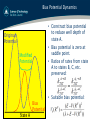
Bias Potential Dynamics
Original
Potential
Modified
Potential
State A
Bias Potential
•  Construct bias potential
to reduce well depth of
state A.
•  Bias potential is zero at
saddle point.
•  Ratios of rates from state
A to states B, C, etc.
preserved:
•  Suitable bias potential:
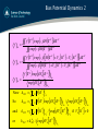
Bias Potential Dynamics 2
f (Γ )exp(− β H (Γ ))dΓ
∫∫
=
∫∫ exp(− βH (Γ ))dΓ
f (Γ )exp(− β [H (Γ ) + V (R ) − V (R )]) dΓ
∫∫
=
∫∫ exp(− β [H (Γ )+ V (R )− V (R )]) dΓ
N
f
A
N
N
N
f
N
N
N
N
A
N
A
=
N
b
N
N
b
f
N
b
N
b
[ ])
exp(β V [R ])
= V δ (R )
= V δ (R )exp(β V [R ])
/ exp(β V [R ])
= V δ (R )
/ exp(β V [R ])
if V [R ] = 0
=k
/ exp(β V [R ])
( )
(
f Γ N exp β Vb R N
Ab
N
b
Now kTST
So
kTST
and
kTST
or
kTST
Ab
*
N
A
*
N
N
N
b
Ab
*
N
Ab
TST
b
N
b
Ab
N
b
Ab
Ab
*
Ab
b
Temperature Accelerated Dynamics
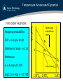
First order reactions:
log(1/τ)
Hopping probability:
P dt = k exp(-kt) dt
Lifetime of state: τ=1/k
Arrhenius:
k = A exp(-E*/RT)
log(1/τ) = log A - E*/RT
increasing simulation
time
p1
δ
p2
E2
stop time tend
1/RToo 1/RTh
E1
1/RTl
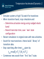
Temperature Accelerated Dynamics 2
•  Simulate system at high T & watch for transitions
•  When transition found, stop simulation and:
-  Determine activation energy using nudged elastic
band
-  Record transition time, save `new’ state
configuration
•  Restart simulation in original state with new velocities.
•  Search for new transitions. Hence build `library’ of
transition data.
•  Stop searching after time tend given by:
tend=exp[E2+(Th-Tl)(E2-δ)/Th]
•  Commence new search from `first’ low T state.
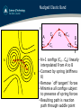
Nudged Elastic Band
E
A
C0
C2
C1
C3
C4
CN-1
B
CN
R
A
B
• N+1 configs (C0…CN) linearly
interpolated From A to B
• Connect by spring (stiffness
K)
• Remove `off tangent’ forces
• Minimise all configs subject
to presence of spring forces
• Resulting path is reaction
path through saddle point
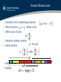
Kinetic Monte Carlo
•  Simulate set of competing processes
•  Rate of process pi is ri (make a list).
•  Define sum of rates
N
R = ∑ ri
•  Generate random number
•  Select process
i =1
u : 0 < u ≤1
⎧ i −1 ⎫
⎧ i ⎫
pi : ⎨∑ rj ⎬ < uR < ⎨∑ rj ⎬
⎩ j =1 ⎭
⎩ j =1 ⎭
R
•  Advance time
•  Repeat!
uR
Δt = − log(u ) / R
pi
{pi ; i = 1,!, N }
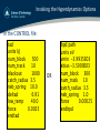
Invoking the Hyperdynamics Options
In the CONTROL file:
tad
units kJ
num_block
500
num_track
10
blackout
1000
catch_radius 3.5
neb_spring 10.0
deltad
6.91
low_temp
40.0
force
0.0025
endtad
OR
bpd path
units eV
vmin -3.9935E03
ebias -3.5000E03
num_block
300
num_track
10
catch_radius 3.5
neb_spring 1.0
force
0.00025
endbpd
Hyperdynamics Files
Additional files for TAD and Bias potential
dynamics:
•  HYPRES/HYPOLD – restart files
•  EVENTS –program activity report
•  CFGBSNnn – Basin CONFIG files (new states)
•  PROnn.XY – Reaction path profiles
•  CFGTRAnn – Tracking CONFIG files
Subdirectories required in execute directory:
BASINS, PROFILES, TRACKS
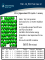
TAD – DL_POLY Test Case 32
255 L-J Argon atoms FCC crystal + 1 vacancy
•  Atoms `hop’ into vacancies
•  Each vacancy has 12 nearest neighbour
atoms
•  So 12 possible escapes from PE basin
•  Use TAD to find them!
•  Use NEB to find activation energy
•  Extrapolate to low temperature for low
T rate
•  Put results into KMC simulation
EVENTS file extract:
Event
nΔt
TRA
38500
TRA
55500
TRA 127500
TRA 750500
Basins Nt
0
1
1
0
2
1
0
3
1
0
4
1
ΔE
7.28338E+00
7.20808E+00
7.28160E+00
7.19597E+00
Time(ps)
3.82250E+01
5.49650E+01
1.26145E+02
7.47515E+02
Extrap.(ps) Stop time(ps)
4.31244E+07 2.04398E+03
5.36891E+07 2.04398E+03
1.41830E+08 2.04398E+03
7.13444E+08 2.04398E+03
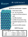
BPD – DL_POLY Test Case 33
998 NaCl ions rocksalt crystal + 2 vacancies
•  Overall neutral system
•  Ions `hop’ into vacancies
•  Escapes from PE basin unknown (a
priori)
•  Use BPD to find them!
•  Use NEB to find activation energy
•  Extrapolate hopping time for zero
bias
•  Put results into KMC simulation
EVENTS file extract:
Event
nΔt
TRA
4500
TRA 399300
TRA 466500
Basins Nt
ΔE
Time(ps)
0
1
1 6.74301E-01 4.39500E+00
1
2
1 1.11127E+00 3.99185E+02
2
3
1 6.57466E-01 4.66495E+02
Extrap.(ps)
7.34793E+03
6.45155E+05
7.53837E+05
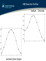
NEB Reaction Profiles
Sodium Chloride
Lennard Jones Argon
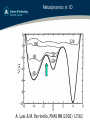
Metadynamics
Metadynamics is a method devised by Alessandro Laio
and Michele Parrinello for accelerating the exploration of a
free energy landscape as the function of collective
variables.
Method:
•  The system potential energy is augmented by a timedependent bias potential consisting of Gaussian
functions of the collective variables
•  The longer a simulation remains in a particular free
energy minimum, the larger the bias potential becomes
– thus forcing the system to seek out a new
thermodynamic state.
•  The accumulated bias potential provides a description
of the free energy surface
Metadynamics in 1D
A. Laio & M. Parrinello, PNAS 99 (2002) 12562
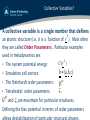
Collective Variables?
A collective variable is a single number that defines
N
an atomic structure (i.e. it is a function of r ). Most often
they are called Order Parameters. Particular examples
used in metadynamics are:
N
•  The system potential energy:
U (r )
•  Simulation cell vectors:
h = ( a , b, c )
•  The Steinhardt order parameters:
Qℓαβ
ζα
•  Tetrahedral order parameters:
Qℓαβ and ζ α are maximum for particular structures.
Defining the bias potential in terms of order parameters
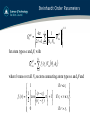
Metadynamics Formulae
M
{
N
N
N
}
Order parameter vector: s (r ) = s1 (r ), !, sM (r )
pi2
N
M
N
System Hamiltonian: H = ∑ 2m + U (r ) + V [ s (r ), t ]
i =1
i
N
Ng
2
M
M
2 ⎤
⎡
V
[
s
(
r
),
t
]
=
W
exp
−
s
(
τ
)
−
s
(
t
)
/
2
δ
h
Bias Potential:
∑
k
⎢
⎥⎦
⎣
k =1
M
n
W and δh are chosen to `fill’ surface at acceptable rate
Force:
M
∂V
N
f i = −∇iU (r ) − ∑ ∇i s j (r )
j =1 ∂s j
N
Free Energy Surface: F ( s M ) = − lim V [ s M (r N ), t ]
g
t →∞
Metadynamics Files
•  METADYNAMICS
-  Data defining the metadynamics hypersurface
•  STEINHARDT
-  Defines the Steinhardt order parameters
•  ZETA
-  Defines the tetrahedral order parameters
Steinhardt Order Parameters
⎡ 4π ℓ
αβ
1
Q = ⎢
Q ℓm
∑
⎢⎣ 2ℓ + 1 m= − ℓ N C Nα
for atom types α and β , with
αβ
ℓ
αβ
2 1/ 2
⎤
⎥
⎥⎦
Nb
Q ℓm = ∑ f c (rb )Yℓm (θ b , φb )
b =1
where b runs over all N b vectors connecting atom types α and β and
if r ≤ r1 ⎫
⎧ 1
⎪⎪ 1 ⎧ ⎡ (r − r ) ⎤ ⎫
⎪⎪
1
f c (r ) = ⎨ ⎨cos⎢
π ⎥ + 1⎬ if r1 < r ≤ r2 ⎬
⎪ 2 ⎩ ⎣ (r2 − r1 ) ⎦ ⎭
⎪
⎪⎩ 0
if r > r2 ⎪⎭
Tetrahedral Order Parameters
1
Tα =
N c Nα
Nα Nα Nα
∑∑∑ f (r ) f (r )(cosθ
c
ij
c
ik
jik
+ 1 / 3)
2
i =1 j ≠ i k > j
Where i, j, k run over all Nα atoms of species α
and N c is the number of pairs of atoms linked to
atom α (assuming all atoms are of type α )
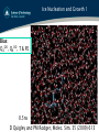
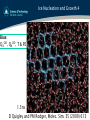
Ice Nucleation and Growth 1
Bias:
Q4OO, Q6OO, T & PE
0.5ns
D Quigley and PM Rodger, Molec. Sim. 35 (2009) 613
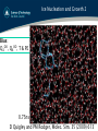
Ice Nucleation and Growth 2
Bias:
Q4OO, Q6OO, T & PE
0.75ns
D Quigley and PM Rodger, Molec. Sim. 35 (2009) 613
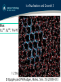
Ice Nucleation and Growth 3
Bias:
Q4OO, Q6OO, T & PE
1.25ns
D Quigley and PM Rodger, Molec. Sim. 35 (2009) 613
Ice Nucleation and Growth 4
Bias:
Q4OO, Q6OO, T & PE
1.5ns
D Quigley and PM Rodger, Molec. Sim. 35 (2009) 613
Conclusions
•  DL_POLY Classic is free
•  It's very versatile with advanced features
•  Go get it!
Part 7
The DL_POLY Java GUI
W. Smith
GUI Overview
•  Java is Free!
•  Facilitate use of code
•  Selection of options (control of capability)
•  Construct (model) input files
•  Control of job submission
•  Analysis of output
•  Portable and easily extended by user
Compiling/Editing the GUI
•  Edit source in java directory
•  Edit using vi, emacs, nano, gedit, whatever
•  Compile in java directory:
javac *.java
jar -cfm GUI.jar manifesto *.class
•  Executable is GUI.jar
•  But.....
****Don't Panic!****
The GUI.jar file is provided in the download or may be not
Invoking the GUI
•  Invoke the GUI from within the execute directory
(or equivalent):
java -jar ../java/GUI.jar
•  Colour scheme options:
java -jar ../java/GUI.jar –colourscheme
with colourscheme one of:
monet, vangoch, picasso, cezanne, mondrian
(default picasso).
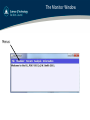
The Monitor Window
Menus
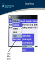
Using Menus
Show
Editor
Option
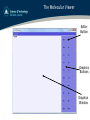
The Molecular Viewer
Editor
Button
Graphics
Buttons
Graphics
Window
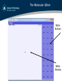
The Molecular Editor
Editor
Buttons
Editor
Window
Available Menus
•  File - Simple file manipulation, exit etc.
•  FileMaker - make input files:
–  CONTROL, FIELD, CONFIG, TABLE
•  Execute
–  Select/store input files, run job
•  Analysis
–  Static, dynamic,statistics,viewing,plotting
•  Information
–  Licence, Force Field files, disclaimers etc.
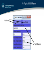
A Typical GUI Panel
Buttons
Text Boxes
DL_POLY & VMD
•  VMD is a free software package for visualising MD
data.
•  Website: http://www.ks.uiuc.edu/Research/vmd/
•  Useful for viewing snapshots and movies.
–  A plug in is available for DL_POLY HISTORY files
–  Otherwise convert HISTORY to XYZ or PDB format
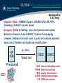
DL_FIELD – http://www.ccp5.ac.uk/DL_FIELD/
Developed by
C.W. Yong
•  Orgainic Fields – AMBER+Glycam, CHARM, OPLS-AA, PCFF,
Drieding, CHARM19 (united atom)
•  Inorganic Fields including a core-shell polarisation option
•  Solvation Features, Auto-CONNECT feature for mapping
complex random structures such as gels and random polymers
•  input units freedom and molecular rigidification
xyz
PDB
Protonated
SOD
DL_FIELD
‘black box’
FIELD CONFIG
4382
19400
7993
13000
730
atoms (excluding water)
bond interactions
angles interactions
dihedral interactions
VDW intearctions
“Hands-On Session”
This will consist of (up to) five components:
•  Download & compile DL_POLY_4&Classic
•  A demonstration of the Java GUI
•  Trying some DL_POLY simulations:
–  prepared exercises, or
–  creative play
•  DL_POLY clinic - what’s up doc?
•  Group therapy – all for one and one for all …
DL_POLY Hands-On
http://www.ccp5.ac.uk/DL_POLY/TUTORIAL/EXERCISES/index.html