Download MORTPAK FOR WINDOWS - the United Nations

POP/SW/MORTPAK/2003
15 September 2003
Update 25 April 2013
MORTPAK FOR WINDOWS
(Version 4.3)
United Nations
New York, 2013
Preface
The present volume contains the working manual for MORTPAK for Windows,
the United Nations software package for demographic measurement in developing
countries. The MORTPAK software packages for demographic measurement have had
widespread use throughout research institutions in developing and developed countries
since their introduction in 1988. Version 4.0 of MORTPAK included 17 applications in
the areas of population projection, life-table and stable-population construction,
graduation of mortality data, indirect mortality estimation, indirect fertility estimation,
and other indirect procedures for evaluating age distributions and the completeness of
censuses. Version 4.3 of MORTPAK enhanced many of the original applications and
added 3 more to bring the total to 20 applications. The package incorporates techniques
that take advantage of the United Nations model life tables and generalized stablepopulation equations. The package, as presented here, has been constructed with
worksheet-style, full screen data entry which takes advantage of the interactive
microcomputer environment and reduces dependence on a manual.
The Population Division of the Department of Economic and Social Affairs of the
United Nations Secretariat has long conducted demographic estimation and projection
activities at the country level, incorporating methodological advances in the construction
of model life tables, for example. As a by-product of these activities, this extensive body
of computer software has been developed. MORTPAK has already been well tested and
is now widely used for analysis of developing country data and in developing country
institutions. The design of the applications in MORTPAK as well as the program
MATCH has its origins in the United States Census Bureau package, Computer Programs
for Demographic Analysis (Arriaga, Anderson and Heligman, 1976).
The Population Division would be pleased to receive comments on experiences
using MORTPAK that would enhance the international usefulness of future software
development activities. Please contact: the Director, Population Division, Department of
Economic and Social Affairs, United Nations, New York, New York 10017, USA.
iii
CONTENTS
Page
Preface................................................................................................
INTRODUCTION
A. The Demographic Procedures..........................................
B. What’s New in MORTPAK for Windows.......................
C. Layout of the Volume ......................................................
I.
1
4
6
USING MORTPAK FOR WINDOWS
A.
B.
C.
D.
II.
iii
Getting Started .................................................................
The Menus .......................................................................
The Worksheets ...............................................................
Special Issues ...................................................................
7
8
17
18
DESCRIPTION OF THE PROCEDURES
A. BENHR
Estimation of completeness of adult death
registration .................................................................
B. BESTFT
Principal component fit to United Nations model
life tables....................................................................
C. CEBCS
Indirection estimation of infant and child mortality ..
D. CENCT
Estimation of completeness of censuses….. ..............
E. COMBIN
Calculation of a life table from life expectancy at age
20 and an estimate of early age survivorship ……....
F. COMPAR
Comparison of empirical mortality rates to those from
model life tables …………………………………
G. CORMOR
Display corresponding probabilities of dying for
selected age groups ...................................................
H. FERTCB
Estimation of age-specific fertility rates from data on
children ever born ......................................................
iv
22
25
27
29
33
35
37
38
Page
I. FERTPF
Estimation of age-specific fertility rates from data on
children ever born and the age pattern of fertility......….
J. ICM
Estimation of single-year probabilities of dying
from ages under five ..................................................….
K. LIFTB
Construction of a life table ........................................….
L. MATCH
Calculation of a model life table ...............................…..
M. ORPHAN
Indirect estimation of female adult mortality from
orphanhood data ........................................................…..
N. PRESTO
Integrated estimation of intercensal mortality,
fertility and age distribution.......................................…..
O. PROJCT
Calculation of a population projection.......................…..
P. QFIVE
Indirect estimation of infant and under 5 mortality
based on model life tables ..........................................…..
Q. STABLE
Calculation of a stable population..............................……
R. TIMSER
Display a time series of a selected model life table column
corresponding to a input series of mortality levels ………
S. UNABR
Graduation of a set of age-specific probabilities
of dying ......................................................................…….
T. WIDOW
Indirect estimation of male and female adult
mortality from widowhood data.................................……..
References..........................................................................................……...
v
40
43
44
47
50
52
56
61
63
65
67
69
72
INTRODUCTION
A. The Demographic Procedures
The present volume presents a set of 20 computer programs for undertaking
demographic analyses in developing countries, including empirical and model life-table
construction, graduation of mortality data, mortality and fertility estimation, evaluation of
census coverage and age distributions and population projections. The 20 demographic
procedures included have been selected by the Population Division as useful for
evaluating demographic data from censuses and surveys and preparing reliable estimates
of demographic parameters. These procedures incorporate techniques for evaluation and
estimation of demographic data, particularly those techniques that incorporate the United
Nations model life-table system (United Nations, 1982) and generalized stable population
equations (Preston and Coale, 1982).
When selecting a new application from the menu, a window in table form presents
a brief description of the procedures, categorized according to their major functions: lifetable and stable population construction, model life table construction, graduation of
mortality data, indirect mortality estimation, indirect fertility estimation, other estimation
procedures and population projections. The package emphasizes mortality estimation,
reflecting the larger number of techniques available and the further advanced mortality
estimation is, compared to that of other demographic components. (Of the nine chapters
in the United Nations manual on Indirect Techniques for Demographic Estimation
(United Nations, 1983), five are dedicated solely. and two partially, to mortality
analysis.)
The LIFTB and STABLE programs calculate empirical life tables and stable
populations respectively based on age-specific mortality rates, plus, in the latter case, an
intrinsic growth rate. The life-table method used is based on the approach of Greville
(1943), which permits calculation of age-specific separation factors based on the age
pattern of the mortality rates themselves. It is, hence, potentially more accurate than
methods which assume constant separation factors, and more robust, under developing
country circumstances, than methods which estimate separation factors based on
population age distributions. Although fertility decline is rendering calculation of stable
populations less applicable for many countries, for others fertility has changed little and
stable population analysis remains useful for evaluation of age distributions and rough
approximation of birth and death rates. However, for countries whose fertility decline is
recent and mortality change has not greatly altered the adult age distribution, STABLE
1
could be useful for evaluating age distributions and studying population dynamics among
adults. In addition, the STABLE program is useful for static simulation of the effects of
changed growth rates and/or mortality rates on age distribution.
The applications MATCH, COMPAR and BESTFT construct model life tables
and compare or graduate empirical data with respect to a model life table. The procedure
MATCH not only generates any United Nations or Coale and Demeny model life table
but also enables the entering of a user-designated mortality pattern which then can be
adjusted to correspond to any desired level. This user-designated model may be a pattern
from a third model life-table system such as the Brass standard (Brass and others. 1968)
but. perhaps, most importantly can be an age pattern of mortality for a particular country.
In the latter case a demographer can generate a model life-table system specific for a
country of interest by using MATCH to construct a series of life tables at different levels
of life expectancy. all consistent with the country's average pattern. Comparison of an
empirical set of age-specific mortality rates to model life-table patterns, through
COMPAR, aids the demographer in the choice of a model life table. However, as data
quality improves, the demographer will wish to retain as many characteristics of the
original data as possible. COMPAR is then very useful for examining deviations of
empirical mortality patterns from the models due to either true differences in age patterns
or to data errors. Similarly, BESTFT offers the opportunity to graduate observed agespecific mortality rates with respect to a model life table (standard), either to smooth a
series of observed rates or to estimate consistent rates for age groups in which data are
lacking.
The procedures UNABR and ICM graduate mortality rates in traditional age
grouping into single year values; UNABR considers the entire age range and ICM under
age 10 only. The procedures are of immediate use when undertaking single-year
population projections or special studies of specific age groups such as the school-age
population or the elderly.
The next group of programs all relate to indirect estimation of demographic
parameters. The five procedures of CEBCS, ORPHAN, WIDOW, COMBIN and BENHR
are mortality-specific. CEBCS provides estimates of infant and child mortality based on
data of children ever born and children surviving tabulated by duration of her marriage.
Data tabulation by age of mother is no longer available within CEBCS because it was
replaced by the QFIVE procedure. ORPHAN and WIDOW carry out variations of the
maternal orphanhood or widowhood techniques to estimate levels of adult mortality. The
procedure COMBIN "combines" early age mortality estimates (perhaps produced by
CEBCS) with adult mortality estimates (perhaps produced by ORPHAN and WIDOW)
and produces a full, consistent life table. The technique BENHR is an application of the
Bennett-Horiuchi (1981) technique; it exploits the generalized stable population equation
to estimate the completeness of death registration using population age distributions from
two censuses and intercensal registered deaths.
Two fertility estimation techniques are included. FERTCB estimates age-specific
fertility rates based on tabulations of average number of children ever born by age of
2
woman. The essential methodology was developed by G. Mortara (1949). The variation
included here was proposed by Arriaga (1983); it has the advantage of providing
estimates of fertility change over time. In the same 1983 article, Arriaga presented an
extension of the P/F technique originally developed by Brass (Brass and others, 1968).
The Arriaga extension, presented in FERTPF, allows the demographer to estimate
fertility at two points in time under conditions of fertility change. Children ever born data
and the pattern of age-specific fertility is necessary from two enumerations when fertility
has not been constant.
CENCT and PRESTO provide techniques for evaluating relative coverage and
age recording in censuses, as well as estimates of intercensal mortality and fertility.
CENCT provides an estimate of the coverage of one census relative to another and hence
is an important first step before applying other estimation techniques which assume
consistency in coverage between two censuses (such as BENHR and PRESTO). Based
on two populations, tabulated by age, and the appropriate model life table, PRESTO
enacts the "integrated method" developed by Preston (1983), providing consistent
estimates of the birth rate, life expectancy and intercensal age distributions. Finally a
simple and easy-to-use population projection program is included.
PROJCT carries out a single-year projection of a population by age and sex, based
on initial male and female populations in five-year age groups and assumed levels and
changes in fertility, mortality and migration.
CORMOR, QFIVE and TIMSER are new applications added to version 4.3 of
MORTPAK. CORMOR calculates and displays corresponding probabilities of dying for
selected age groups and for all nine model life tables. TIMSER calculates and displays a
time series of a selected model life table column corresponding to an input series of
mortality levels. QFIVE estimates infant mortality and under 5 mortality by applying the
two versions of the Brass method: the Trussell version based on the Coale-Demeny
model life tables and the Palloni-Heligman version based on the United Nations model
life tables. QFIVE was previously distributed (for DOS operating system) together with
the manual “Step-by-Step Guide to the Estimation of Child Mortality”, which is available
for download.
3
B. What’s new in MORTPAK for Windows
Version 4.0
Data entry is now on worksheets that resemble spreadsheets, but do not have the
functionality of a full spreadsheet. These worksheets were designed to easily copy data
to and from your spreadsheet. For example, after creating a new worksheet, a user might
copy some of the data from a spreadsheet and paste it into the worksheet. After running
the selected MORTPAK application, all or part of the results can be copied and pasted
into a spreadsheet for further calculation or for creating graphs.
Output data now has two styles. The traditional MORTPAK style is called
document output. It is ready for exporting to a word processor and printing in a cameraready format. The output is also placed onto the worksheet and is handy for copying
results into a spreadsheet.
Some applications were enhanced. LIFTB can accept l(x) as input values and
outputs can have any open age group, regardless of input data. A larger open age group
will result in the output table being extrapolated. Large extrapolations should be done
with caution. Check the output thoroughly. PROJECT now uses migration data.
The older versions of MORTPAK used data files with fixed width data fields,
which limited the size and precision of the numbers. The data in the new input data files
can have any size or precision. The worksheets often have a display format set for
selected columns. Internally, these numbers retain all their significant digits. To see the
unformatted number, put the worksheet cell into edit mode (by pressing F2 or doubleclicking on the cell) or copy the data to a location having a different display format.
Version 4.3
MORTPAK can now perform batch runs from one or more input data files. The
data files must be version 4.0 or later because earlier versions do not contain the
application name within the data file. The batch runs can be initiated from “Run” on the
main menu. The output data files can be produced in one of two styles: one output file
created from each input file or the output data can be merged into one file. The output
data uses comma separated value format (i.e. *.csv) so that they can be ready for import
into spreadsheets and databases. The first line is a column header used to define the data
fields. Many of the input data parameters are repeated in each line of the output, similar
to many databases. This is useful if sorting and filtering data within the spreadsheet. The
following applications support batch runs at this time: BESTFT, CEBCS, FERTCB,
FERTPF, ICM, LIFTB, MATCH, QFIVE and UNABR. The other applications cannot
produce batch runs.
4
For many applications, a summary table containing probabilities of dying are now printed
in the output worksheet. The selected indicators 1q0, 4q1, 5q0, 20q15, 35q15, 45q15,
40q30 and 20q60 are displayed, if not already in other parts of the output
Enhancements to the outputs only appear in the MORTPAK worksheets. Document style
output, which produces word processing style output similar to MORTPAK 3, is no
longer supported and is no longer being updated.
5
C. Layout of the Volume
This introduction is followed by two chapters. Chapter I describes the Windowsbased interface. It explains how to get started with using MORTPAK, a description of
each menu and sub-menu entry, and how to use the worksheets and the distinctive
features of the worksheets. Finally, it covers special issues that may need special
attention.
Chapter II describes the 20 MORTPAK applications (procedures). It describes
the purpose of each procedure, a mathematical and demographic description of the
technique, the data required and a description of applying the technique with sample
input data (that is provided with the package).
6
I. USING MORTPAK FOR WINDOWS
A. Getting Started
To enter new data and run a MORTPAK application
Select "new" from the FILE menu and choose the application. A description of
each application is supplied. For those who are familiar with the application names, an
alternative is to select the application from the APPLICATION menu. At the bottom of
the list, clicking "Description" will open up a form containing the application names and
their description. Once the worksheet is open, enter the data in the shaded areas allocated
for input. Click the RUN button above the worksheet. To save the input data and/or
output data, choose "save as" from the FILE menu. For help specific to the worksheet,
click on the "Data Entry Help" button or go to the help menu.
To modify existing data and run a MORTPAK application
Select "open" from the FILE menu and select the input file. When the worksheet
appears, make any modifications to the input data in the shaded areas allocated for input.
Click the RUN button above the worksheet. To save the input data and/or output data,
choose "save" from the FILE menu. For help specific to the worksheet, click on the
"Data Entry Help" button or go to the help menu.
To import from versions of MORTPAK prior to 4.0 and run a MORTPAK
application
Select "open" from the FILE menu and select the input file. MORTPAK for
Windows will automatically recognize that the file is from a previous version of
MORTPAK and will ask you to indicate the application name. A MORTPAK for
Windows worksheet will open with the imported input data in the shaded areas allocated
for input. Click the RUN button above the worksheet. To save the input data and/or
output data, choose "save as" from the FILE menu. For help specific to the worksheet,
click on the "Data Entry Help" button or go to the HELP menu.
7
B. The Menus
When MORTPAK starts, a “Getting Started” window appears on the
screen (see previous page). Most menu item will automatically close this screen.
If needed again, see the help menu. When opening a worksheet, two command
buttons are on the form. “Data Entry Help” opens an application specific help
window and is also available in the menu. The button labeled “Show Document
Output” is for opening and closing the document output window. Some menu
items refer to only the worksheet or only the document output. For example,
“Copy from Worksheet” will not copy data from document output. “Copy from
Document Output” is a separate menu item.
On the tool bar, a “W” or “D” is placed within the print and copy icons to
distinguish between the worksheet or document output. Since the document
output is not editable, commands such as cut and paste refer to the worksheet
only.
File
New
Opens up a new worksheet with no data entered.
Since each application has a different layout for entering data and viewing
output results, an application name must first be chosen. Prior to opening
the worksheet, an application selection form appears. The initial list is in
alphabetical order and can be scrolled using a scroll bar. This list can be
shortened by selecting one of the groups at the top of the form. Lower in the
form, application names are listed on the left, with a description in the
middle and a selection button to the right.
Open Opens a dialog box for selecting the input file name. Starting with version
4.0 of MORTPAK for Windows, the default file extension is *.MPL. The
input file internally contains the application name associated with the input
data. Simply choosing the file name will open the correctly formatted
worksheet and fill in the input data into the correct location. Data from
earlier versions of MORTPAK (before version 4.0) can also be opened, but
does not contain the application name within the file. Therefore, the
application name must be given before the data is imported into the
worksheet. This data can be saved in the new format by using “Save As”
from the menu.
Note: the number of open worksheets is limited to 25.
Close This command closes the currently active worksheet.
______________
8
Save Input Data Saves the currently active worksheet without changing the
current file name. Whenever a new worksheet is created (input data is
blank), it has no file name. The listed file name will be “Untitled.MPL”. To
save these worksheets, a file name must be given. If file “Save” is chosen
instead of file “Save As”, MORTPAK will automatically switch to file
“Save As”.
Save Input Data As Saves the currently active worksheet. A dialog box opens
with the current file name as a default. Any name can be chosen except
“Untitled.MPL” or the name used by another open worksheet.
Save Document Output (*.rtf) The document output is in a format similar to early
versions of MORTPAK. The advantage of saving document output as an
RTF file is that it keeps some of the word processing formats. It can easily
be imported into a word processor that can open RTF files.
________________
Page Setup For setting print margins and selecting the portrait or landscape page
orientation. Can also select another printer, paper source and paper size. For
page setup to function, at least one printer driver must be installed.
Print Worksheet …
Print Preview
Shows how the output will appear before printing. This
follows the same format at “Print Worksheet” below. Not
all worksheet cells are printed. The cells selected for
printing are pre-determined for each application. For
customized selections, highlight the cells and print with
“Print Selection” from the menu. Selected pages can also
be printed from here.
Print Worksheet For printing a predetermined area of the currently active
worksheet. The predetermined print area is chosen specific
for each application. A dialog box will appear for selecting
a printer, selecting paper source and paper size or setting
portrait or landscape page orientation. For setting margins,
use “Page Setup”. For printing a customized selection of
cells, use “Print Selection”.
Print Selection
For printing selected areas of the worksheet. These appear
highlighted on the worksheet.
9
Print Selected Pages Use this for printing selected pages. If unsure of the
page numbers, use print preview and print the selected
pages from there.
________________
Print Document Output For printing document output. Choose the smallest font
size if the output table is wide and the paper is in portrait mode. For better
results, it is recommended to first export into a word processor and
customize the output for best appearance.
________________
Last four input files This group contains the last four input files that were
opened. As a convenience, press any of these to open the input file. For a
new installation of MORTPAK, this group will appear empty.
________________
Exit
To exit MORTPAK.
Edit
Undo Whenever data is cut from or pasted to the worksheet, MORTPAK will first
save the grid contents in case it is necessary to undo the change. If a
worksheet cell is not being edited when Undo is pressed, Undo will restore
the worksheet to what was saved previously. If a worksheet cell is being
edited, Undo will restore only that cell to its previous contents.
__________
Select All Worksheet Cells Every cell is selected and highlighted. This is
useful for copying the entire worksheet to the clipboard and later pasting it
into a spreadsheet.
Cut from Worksheet Places data from highlighted cells onto the clipboard and
erases only those cells that are not in protected areas. This data may later be
pasted into any worksheet or external spreadsheet.
Copy from Worksheet Copies data from highlighted cells to the clipboard. This
data may later be pasted into any worksheet or external spreadsheet.
Paste to Worksheet Pastes data from the clipboard into unprotected areas of the
worksheet. The data on the clipboard may be from any worksheet or from
an external spreadsheet. When pasted from an external spreadsheet, only
the values will be pasted (i.e. the formula was not copied).
10
Paste, Transposed to Worksheet Pastes data from the clipboard to unprotected
areas of the worksheet, but reverses rows and columns. The data on the
clipboard may be from any worksheet or from an external spreadsheet.
Clear Selection from Worksheet Erases selected cells that are not in protected
areas. Protected cells will be ignored.
Round Off Selected Input Numbers
This function rounds off numbers in
selected cells. Any number of decimal places from 0 through 10 can be
selected. This is useful for unformatted columns of numbers that are
displaying too many digits after the decimal point. This function is used
mainly to improve the appearance of the numbers in the data column.
Selecting a number too low will reduce the data precision.
____________
Select All Document Output The entire document output is highlighted and
ready for copying to the clipboard. After pressing “Copy from Document
Output”, paste into a word processor.
Copy from Document Output Copies data from highlighted areas of document
output to the clipboard. This data may later be pasted into a word processor
document.
Select Font Size for Document Output All newly opened worksheets have the
font size of Document Output set to 8 as a default. The font size can be set
individually for each open worksheet. To change the font size of a
particular Document Output, select one of the worksheets by clicking on it
so that it becomes active. Selecting this menu item will bring up a submenu with the font sizes 6.75, 8, 9, 10 and 11. This will change the font
size of the currently active worksheet only. The font size for newly opened
worksheets will remain at 8. If text is copied to the clipboard from
Document Output and pasted into a word processing document, the font size
will be approximately the same as that chosen above. This menu item is
also available under the View menu.
_____________
Find
For finding data or text in the worksheet or document output. The
worksheet is the default. “Whole word only” and/or “Match case” can be
chosen. Type in the search text and press “Find Next”. When the end is
reached, the search start from the beginning. If the cursor is moved, the
search will start from the position of the cursor.
11
View
Toolbar For selecting whether to display or hide the toolbar. The toolbar is a set
of shortcut icons for selected menu items. The icons available are “New”,
“Open”, “Save”, “Print Worksheet”, “Print Document Output”, “Cut”,
“Copy Worksheet”, “Copy Document Output”, “Paste”, “Run”,
“Display/Update Chart – Standard” and “Find”. A “W” or “D” was placed
into the print and copy icon to distinguish between worksheet and document
output. Icons such as cut and paste apply only to the worksheet because
document output cannot be edited.
Status Bar For selecting whether to display or hide the status bar. The status bar
shows the date and time in the bottom of the screen.
______________
Comment Box The contents of the comment box are for the currently active
worksheet. To view the comments associated with another worksheet,
simply click the desired worksheet to make it active. The contents of the
comment box can be edited and are saved when the data is saved. It is
useful for listing data sources and other issues related to the input data.
______________
Select Font Size for Document Output All newly opened worksheets have the
font size of Document Output set to 8 as a default. The font size can be set
individually for each open worksheet. To change the font size of a
particular Document Output, select one of the worksheets by clicking on it
so that it becomes active. Selecting this menu item will bring up a submenu with the font sizes 6.75, 8, 9, 10 and 11. This will change the font
size of the currently active worksheet only. The font size for newly opened
worksheets will remain at 8. If text is copied to the clipboard from
Document Output and pasted into a word processing document, the font size
will be approximately the same as that chosen above. This menu item is
also available under the Edit menu.
Options Opens up a form with tabs labeled “Select Colors”, “File Locations” and
“General Choices”. Background colors can be changed for worksheet
protected cells and edit cells. A non-active worksheet will not show the new
colors unless the worksheet is closed and re-opened. In the “File Locations”
tab, default file locations can be selected for MORTPAK software and input
data. Whenever MORTPAK is started, the input dialog box opens with the
default path chosen in the “File Locations” tab. Afterwards, the input dialog
12
box opens with the path of the last opened file. If MORTPAK is restarted,
the input dialog box opens with the path from the “File Locations” tab. The
“General Choices” tab has check boxes that are self described. Scale
worksheet column width indicates how wide to make the columns. A value
of 100% is the standard size. If large fonts are chosen (from Windows), it
might be necessary to choose a larger column width so that worksheet cells
will fit within the box. The percentage of the window showing document
style output is also set through the Options menu. All worksheets have two
displays, the worksheet grid and the document output. When the document
output is open and displayed, it can take up 15% to 100% of the screen.
Opened worksheets can later be set individually by dragging the horizontal
bar above document output in the up or down direction.
Application
Application name list This menu item is for selecting new worksheets. For those
familiar with the application names, this is the fastest way to select them.
_________
Description This choice is the same as “New” from the menu. A selection form
is opened with a description of each application name.
Run
When the input data is ready, select “run” from the menu and then choose
“Calculate Output for Selected Worksheet” to process the data, or simply
press the run icon. Whenever “run” is selected, the output is always sent to
the worksheet and to the document output window. The document output
window can be shown or hidden with the toggle button on the worksheet
form. The worksheet output is desirable for exporting data to external
spreadsheets by copying to the clipboard and pasting into the spreadsheet.
The document output is desirable for exporting output to a word processor
for producing printed copies. This output can be printed, copied to the
clipboard or saved as a rich text format (*.RTF) file. The document output
style is similar to early versions of MORTPAK. While the worksheet output
is more suitable for export to spreadsheets, this output is more suitable for
export into a word processor. One way is to copy the data into the clipboard
and paste it into a word processing document. Use “Copy from Document
Output” from the menu or use the shortcut key ctrl-ins. Shortcut keys such
as ctrl-c are for copying data from the worksheet to the clipboard and not
from document output. Another way is to select “Save Document Output”
from the menu. This will save the output as a rich text format (*.RTF) file.
These RTF files retain the displayed formatting and can be opened from
your word processor. From there, the results can be edited for better
presentation on paper. For example, some outputs are too wide to fit within
13
the margins and word wrapping occurs. The page orientation can be
switched from portrait to landscape and margins can be reduced. If
necessary, the font size can be adjusted to better fit the margins.
Starting with version 4.3, batch processing was added to MORTPAK for
selected applications. Batch processing requires data files to be from
version 4.0 or later so MORTPAK can recognize the application
corresponding to the data. If the application does not support batch
processing, a message will be displayed in the output file. When one output
file is desired for each input file, then choose “Select Data to Create CSV
Output files” from the “Run” menu. To merge all the output into one data
file, then choose “Select Data for Merged Output CSV file” from the “Run”
menu. The output data uses comma separated value format (i.e. *.csv) so
that the output data can be ready for import into spreadsheets and databases.
The first row of the output file is a column header to define each column of
the data below it. The output data uses the same style of a database table.
Therefore, many data parameters are repeated in each row. This is useful
for sorting and filtering data within a spreadsheet
Chart
To create a chart, simply highlight the necessary number column of numbers
and then select on of the chart type from the menu. If the highlighted
selection box is square or horizontal, it is no longer assumed the data appear
in columns. Therefore, a dialog box opens asking if the data are in rows or
columns. On the chart window, control buttons appear on the right. The
first one allows the chart header plus the X-axis and Y-axis labels to be
customized. The “Copy as bitmap” button places the graphic image into the
clipboard ready for pasting into any image editing software. The “Copy as
metafile” button is better than bitmaps when pasting into software such as
Word and Excel. To copy the metafiles properly, the software must be
opened before pressing the copy button. Once pasted into external software,
the metafile image can be enlarged without losing resolution. The “Print”
button opens a print preview window to customize the graph before printing.
The “Close” button simply closed the chart window.
Select Chart Type for Icon
The display chart icon on the tool bar is set to line
graph, as a default. This menu item allows the display chart icon to be set to
any of the other chart types. Restarting MORTPAK will set the icon back to
line graph.
Display/Update Chart – Line
column or row of cells.
For making a line graph from the highlighted
14
Display/Update Chart – Bar For making a bar chart from the highlighted
column or row of cells.
Display/Update Chart – Logarithm Same as line graph but the Y-axis is in the
log scale. Invalid data points are set to a value below the lowest valid data
point. A warning is then placed the chart header indicating that the lowest
data point(s) is invalid (i.e. less than or equal to zero). A value closer to
zero was not chosen to prevent the line from having a large downward
spike.
Display/Update Chart – XY Graph The first selected line is the X-axis and the
following selected lines are Y1, Y2, etc. and is displayed as an XY line
graph.
Display/Update Chart – XY Scatter
The first selected series is the X-axis and
the following selected series are Y1, Y2, etc. and are displayed as a marker
for each data point.
Display/Update Chart – Box Plot
plot.
Each series of values is displayed as a box
Display/Update Chart – Pyramid
One or two data series may be selected, the
first appears as bars facing left and the second (if available) to the right.
Both appear as a proportional distribution with the left and right having
equal scale values. The first data point(s) in the sequence is at the bottom
and the last is on the top. The Y-axis shows the sequence number. This
chart is intended for demographers to display population pyramid charts.
Window
When more than one worksheet is open, the worksheets can be “cascaded”,
“tiled horizontal” or “tiled vertical”. “Arrange icons” is for neatly arranging
the icons of minimized worksheets at the bottom of the screen.
____________
All open windows are listed here. Worksheets can be selected here by
clicking on their name.
Help
Contents (Version 4.0) Opens up the original help file. Three tabs are available
to navigate the help file, by table of contents, index or by word search. The
contents tab (default tab) is organized by topic. The index tab list topics in
alphabetical order. The search tab is for finding text located within the
15
topic. All topics having at least one match are then listed. Select the topic
to display. All matches are shown highlighted within the topic.
Updates Since Version 4.0 Opens up the help file which describes the updates
which took place since version 4.0.
Getting Started Opens up the help file and displays the getting started page. This
is intended for new users and is a duplicate of what is shown when
MORTPAK starts up.
Data Entry Help Opens up the help file, with the selected chapter describing the
input variables for the current worksheet. If a worksheet is not open, then
the help file opens with a page describing the data entry help and reminds
the user that an active worksheet needs to be opened first. This help can
also be activated from a command button on the worksheet form.
_______________
How to Print Manual
_______________
Contains instructions for printing the user manual.
About MORTAK Copyright related information for MORTPAK for Windows
(version 4.0).
16
C. The Worksheets
The new MORTPAK worksheets are designed to display the input and output
data. They look similar to spreadsheets, but do not have the functionality of
spreadsheets. Input and output data on the worksheet can be exported to a spreadsheet
program. Simply select and copy the data from the worksheet into the clipboard and
paste it into the spreadsheet.
All worksheets have a grid inserted within the worksheet form. A grid is
specifically designed for each MORTPAK application. The worksheet forms have
common characteristics. The application name is placed within the caption of the
worksheet. Below the caption is the input file name together with the disk drive and path
where the file is located. File names containing “Untitled.MPL” are reserved for files
that were not yet given a name. For example, a new worksheet uses Untitled.MPL to
show that it is waiting for its real name. From the menu use “File”, “Save As” to save the
file onto disk with its correct name. Below the file name is the date when the worksheet
was last updated, or new worksheets, the creation date. To the right is a button called
“Data Entry Help” which opens a floating help window. This help is specific to the
selected application and provides help for data input. For example, it might supply more
details for the column labels including units and valid numeric ranges. Above the grid is
a one line brief description of the selected application.
To the right is a second button that toggles between “Show Document Output”
and “Show Data Entry/Worksheet Output”. Immediately after running an application, the
Data/Entry Worksheet output is exhibited. To see the document output, click on the
button. The document output will cover all or part of the worksheet, depending on the
option chosen. The percentage of the worksheet covered by the document output can be
set in MORTPAK. In the menu, choose “View”, then “Options” and click on the
“General Choices” tab. The percentage of the worksheet covered by the document output
can be set to any number between 15 per cent and 100 per cent.
The space on the screen allotted to the worksheet and document output can also
be adjusted by moving the cursor above the document output so that the cursor changes
into and up-and-down arrow. Then drag the divider lower or higher as desired.
The grid uses three colors. One color is for protected cells. These cells have data
labels and cannot be overridden. Another color is for input data. These fields show
where input data is to be placed. Below the protected area are cells with a white
background. This area is provided as a general working or storage area. For example, a
table can be made in this area from a series of outputs. For example, an input value can
be repeatedly incremented and part of the output can be copied to the white areas of the
worksheet. Then the user can analyze how the output relates to the input. For fancier
graphs or data calculations, this table can then be copied to the clipboard and pasted into
a spreadsheet.
17
D. Special Issues
At the bottom of the worksheet, a special working area is provided for the user. It
is not intended as a spreadsheet but is useful for “holding” data. For example, if a series
of outputs is generated, columns of numbers can be copied into the special working area
for comparison or for creating a table, which can later be exported into a proper
spreadsheet.
Even though the worksheet is not a spreadsheet, it has some of its characteristics.
For example, if the number of characters or digits for a cell is too many to be viewed
within that cell, there will be spillover into empty cells on the right, giving the
appearance of a long “merged cell”. (If the cells to the right are not empty, the full
contents of the cell cannot be shown and will have a “…” at the end.) However, the cells
are not truly merged and if the cursor is moved into one of the “spillover cells” on the
right, text or data can be entered. When the cursor has been moved into one of the
spillover cells, a marker line is placed under the selected cell to indicate the location.
For cells containing drop down lists (e.g., to select “males” or “females”), the size
of the cell will adjust to match the width needed by the data choice. If predefined labels
are too big to fit in a cell, it is possible the Windows font size was set to a larger size than
the default. To increase the column width of newly opened worksheets, from the menu,
choose “View” and “Options” to increase the default column width.
It is possible to adjust the width of individual columns within an open worksheet.
Above each column of cells is a narrow bar with dividing lines. Moving the mouse
cursor over the dividing line will change the cursor into two arrows facing left and right.
Press and hold the left mouse button and drag the line left or right to resize the column.
When running an application, the output is always saved as worksheet format, as
well as document output format in a rich text format (*.RTF). Both are used because
they have different characteristics. The worksheet output is desirable because it has
characteristics similar to a spreadsheet. It is easy to copy data to the clipboard, which is
ready for pasting into the spreadsheet. The RTF file is desirable because it has a style
suitable for exporting into a word processor and has an output presentation similar to
earlier versions of MORTPAK. It can be displayed by pressing the “Show Document
Output” button above the worksheet. Pressing the same button again (now labeled
“Show Data Entry/Worksheet Output”) will close the document output window.
The document output can be printed directly or for customized printouts from a
word processor, the document output can be copied to the clipboard or saved as a rich
text format (*.RTF) file. The data from the clipboard can be pasted into an existing word
processing document or the word processor can open the saved RTF file. The output uses
a font called “Courier New” because each character has the same width. This is useful
for lining up table columns without using tabs. The output can be customized by making
the font size smaller to fit the margins or larger for easier viewing. Because this output
18
does not use tabs, the table formatting will remain the same. For outputs that are too
wide to fit the margins, the page orientation can be switched from portrait to landscape.
Page breaks are marked with a $ sign. For long outputs, search for the $ sign and replace
it with a page break. Word processors have search and replace feature. For Microsoft
Word, put $ in the search box and put ^m in the replace box to replace each $ with a page
break.
When the document output window is open, it can use 15% to 100% of the
screen. A value of 100% means that the entire worksheet is covered by the document
output. In the menu, choose “View” and “Options” to set the default percentage for
document output. New installations of MORTPAK are set to 100%. This percentage
applies to newly opened worksheets and can be changed for individual worksheets by
dragging the document output window larger or smaller. Move the mouse cursor within
the horizontal bar above document output. When the cursor shows an arrow facing both
up and down, press and hold the left mouse button and drag the document windows to its
desired size.
Whenever “data entry help” is selected, this help file opens to the topic associated
with the active worksheet. To save space on the desktop, the navigation tabs (context,
index and find) are not shown and the topic window is maximized.
The help file for MORTPAK contains two window styles. One style contains
navigation tabs that are useful for selecting a help topic. The other style is context
sensitive and is for either selecting the getting started page or the data description of the
selected application. Both window styles can be resized using standard Windows
techniques. When the help windows are closed and open at a later time, the previous size
of the window is remembered.
Data entered into the worksheets can contain any number of decimal places. The
applications use the full precision when performing the calculations. For better
appearance, data columns in the worksheet are display rounded to a pre-determined
number of decimal places. The full precision of the number can be seen when the cell is
in edit mode (selected by pressing F2 or double-clicking on the cell) or when the data is
saved on disk. The grid used by MORTPAK accepts formatting information for
individual column. Individual cells cannot be formatted separately. In some cases where
more than one type of data is on the same column, it was necessary to leave the column
unformatted. If no formatting is specified, then the right most zeros after the decimal
place are not displayed.
Each worksheet form has an entry for an input file name together with the disk
drive and path where the file is located. File names containing “Untitled.MPL” are
reserved for files that were not yet given a name. For example, a new worksheet is
labeled Untitled.MPL to show that it is waiting for its real name. From the menu use
“File”, “Save As” to save the file onto disk with its new name. Any name can be chosen
except “Untitled.MPL” or the name used by another open worksheet.
19
When entering data into a worksheet, do not add commas. The input file
separates related values with commas. Adding commas to the data will insert additional
commas to the input data file. Therefore, when the file is opened, the numbers will be
split wherever a comma was placed.
Use caution when printing large worksheets, especially for the application
PROJCT. For these it is better to use print preview to select page numbers for printing or
better yet, highlight selected areas and use “print selection”.
Remember that the worksheets are not spreadsheets with auto-calculate on. If
input data is changed, it is necessary to “run” the program to update the output data so
that all input/output is consistent.
Worksheets often contain cells with drop down lists. This is convenient when
choosing from a fixed list of choices. This also ensures proper spelling and consistency
for text inputs. For example, the input field might contain an extra space, abbreviations
might be used or entries might be plural instead of singular.
When a MORTPAK data entry window is active, both the worksheet area and a
Document Output area are active at the same time. Even when the Document Output
area is hidden, (i.e. only the worksheet is shown) it is still active. For example, pressing
the “Run” button will update both the output areas of the worksheet and fill the
Document Output area with the output results. If a menu item applies to only one of the
two areas, its label identifies which area it applies to. If shortcut keys are available, its
definition is shown to the right of the menu command. Since Document Output is not to
be edited by the user, except by pressing the run button, commands such as cut and paste
only apply to the worksheet. The copy command has two shortcut keys, ctrl-c and ctrlins. For MORTPAK, it was decided to use ctrl-c for the worksheet and ctrl-ins for
Document Output. The toolbar contains copy and print icons. A “W” was placed within
the icons that apply to the worksheet and a “D” was place within the icons that apply to
“Document Output.
For applications that generate graphs, such as PRESTO and CENCT, the graph
will be displayed when the “run” button is pressed. The graph can be minimized to see
again later, or the “run” button can be pressed to re-display the graph. The graphs
generated by PRESTO and CENCT both display the age group as a data point. These
graphs can be displayed as XY scatter graphs or XY line graphs. First select the output
data from columns 17 and 18 for CENCT or select the output data from columns 14 and
15 for PRESTO. Then select “Chart” from the menu and then select the chart type.
Large outputs are produced by PROJCT or when MATCH prints multiple output
tables. The entire output is shown in document output but the worksheet has limited
space. Therefore, only one table at a time can be shown in the worksheet. To select
which table to display, a combo box is created on the form containing a drop down list
with an entry for each available table. For example, the combo box for PROJCT has an
entry for each year displayed in the document output. Remember that only the “Run”
20
command updates the output data. The combo box only selects which one of the output
tables to display. If input data is changed, it is necessary to “Run” the application to
update the output tables. Commercial spreadsheets update for every cell change.
MORTPAK uses manual update and updates only when “Calculate Output for Selected
Worksheet” from the “Run” menu is selected or the “Run” icon is pressed.
When a group of cells is selected within a worksheet and a chart type is selected
from the chart menu, it is possible to choose another chart type without first closing the
previous chart window. The newly selected chart uses the data points from the already
selected cells within the currently active worksheet. If you want to make a worksheet
active and retain the current selection, click on the worksheet form outside of the cell
grid. If you click on one of the worksheet cells, the cursor will move there and the
selection will be cancelled.
The shortcut key “ctrl-a” always selects the entire worksheet, but selects all of
document output only when the cursor is in the document output box.
21
II.
DESCRIPTION OF THE PROCEDURES
A. Description of BENHR
Purpose of procedure
Estimates the completeness of adult death registration based on population age
distributions from two censuses and registered deaths by age for the intercensal period.
Description of technique
Bennett and Horiuchi (1981) have shown that, in a closed population, the
observed age distribution of deaths can be used in combination with two population age
distributions and an age-specific growth rate factor to calculate the completeness of death
registration above a certain age x, the age beyond which death registration can be
assumed to be equally complete. The growth rate factors are calculated from age-specific
intercensal population growth rates. The method, essentially, estimates completeness of
death registration by using the growth-rate-transformed registered deaths to generate an
independent estimate of the average intercensal population at an age above x; the ratio of
this figure to that calculated from the two observed censuses provides an estimate of
completeness of death registration above age x. The technique, therefore, provides a
series of estimates of completeness of death registration due to the possibility of varying
x from age 5 through the maximum age. If the two population censuses are equally
complete, if death registration is equally complete for all ages above 5, and if there is no
bias in age statement, this series will provide a more-or-less constant set of figures for
completeness of death registration. Variance from a "constant" set of figures indicates
that one or more of the above conditions does not hold. (Some systematic patterns of
departures from constancy may reflect violations of particular assumptions and thus
suggest appropriate directions for correcting the data (see Preston and others, 1980).)
The computer program calculates the median of the series of estimates and
assumes this median is the best estimate of death registration completeness. This best
estimate is then used to calculate an adjusted set of age-specific death rates and life
expectancies for ages 5 and above.
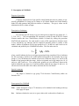
The method requires a preliminary estimate of life expectancy for the oldest age
entered for the population age distribution. (For example, if the population age
distribution has 80+ as the oldest age group entered, a preliminary estimate of life
expectancy at age 80 is required.) This life expectancy is estimated within the computer
program using a set of regression equations which relate life expectancy at age a to the
ratio of registered deaths for age group 60 and over to registered deaths for age group 5
and over. These regressions were estimated from a set of data points simulated from
stable populations generated from male and female model life tables from the United
Nations General Pattern with life expectancy at birth varying from 35 years to 75 years,
22
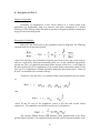
at one-year intervals, in conjunction with intrinsic growth rates varying from .015 to .035,
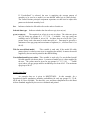
at intervals of .005. The regression equations are
e(60)
e(65)
e(70)
e(75)
e(80)
e(85)
=
=
=
=
=
=
9.345
7.535
6.049
4.890
4.060
3.379
+ 12.403 D60+/D5+
+ 10.072 D60+/D5+
+ 7.918 D60+/D5+
+ 5.965 D60+/D5+
+ 4.162 D60+/D5+
+ 2.836 D60+/D5+
where e(a) is life expectancy at age a, and D60+/D5+ is the ratio of intercensal registered
deaths for age group 60+ to age group 5+.
Data required for BENHR
Title: A heading of up to 72 characters to be printed above the calculated table.
Final open age group: Indicates the final open age group given for the first and second
populations and for the intercensal deaths. The final open age group must be
between 60+ and 85+.
Month of first enumeration: Indicates the month that the first census was taken.
Year of first enumeration: The year the first census was taken; for example, 1960.
Month of second enumeration: Indicates the month that the second census was taken.
Year of second enumeration: The year the second census was taken; for example,
1970.
Population of first census: The population by age for the first census. Data are for age
groups 0-5, 5-10, ..., up through the last open given age group available.
Population of second census: The population by age for the second census. Data are
given for age groups 0-5, 5-10, ..., up through the last open age group available.
Intercensal deaths: Registered deaths for the intercensal period. Data are given for age
groups 0-5, 5-10, ..., up through the last open age group available.
Sample Input Data
An example data set is given in BENHR.MPL. In this example, estimated
completeness of death registration and adjusted life expectancies for a
hypothetical female population are calculated and printed. To calculate the
completeness of death registration, e(80) was estimated to be 5.481 years (see
footnote 1 in the sample output). It is used for calculation purposes only and
23
not intended as the actual life expectancy at age 80. Footnote 2 indicates that
death registration is 0.682 per cent complete; this value is used to adjust the death
rates. These adjusted death rates are then used to calculate the life table.
24
B. Description of BESTFT
Purpose of procedure
To find the one-, two- or three-component United Nations or Coale-Demeny
model life table which best fits one or more probabilities of dying (q(x,n) values) or
m(x,n) given as input.
Description of technique
Using least squares criteria, the United Nations model life table of a given pattern
is found which best fits one or more q(x,n) values given as input. Simply, the procedure
is one of graduation with respect to a standard. When only one q(x,n) value is given, this
program presents results identical to that of the procedure MATCH. The one-component
model life table (i.e., those presented in United Nations, 1982, annex I) is presented, as
well as the adjusted two- and three-component tables. However, at least two q(x,n)
values must be given for estimation of the two-component table and at least three values
for the three-component table. In place of the United Nations model, an alternative
model supplied by the user can be given as input and the best fit of the empirical data to
that model will be calculated (for a more detailed description of the methodology, see
United Nations, 1982, chap. IV). Starting with version 4.3, new United Nations or new
Coale-Demeny models can be selected. The level of these new models is determined by
the closest fit to the input data before the best fit regressions are applied. The new
models also permit m(x,n) to be selected as input.
Data required for BESTFT
Title: A data description of up to 40 characters, to be included in the heading at the top
of the page of output.
Model life table pattern: Indicate the model life table pattern to be used. The choices
are:
User-defined model
UN Latin American model
UN Chilean
UN South Asian
UN Far East Asian
UN General
Coale-Demeny West
Coale-Demeny North
Coale-Demeny East
Coale-Demeny South
25
If “User-defined” is selected, the user is supplying the average pattern of
mortality to be used as a model (see user-defined model q(x,n) values below).
The United Nations principal component equations are then used to adjust this
pattern to the desired mortality level.
Sex:
Indicates whether the life table refers to the male or female sex.
Selected data type:
Indicates whether the data refers to q(x,n) or m(x,n).
q(x,n) or m(x,n):
The empirical set of q(x,n) or m(x,n) values. The values are given
only for those age groups (0-1, 1-5, 5-10, ...) available. Any age group not
available can be left blank or set to 0.0. As these data are read in on a "perperson" basis, each value must be in the interval 0 to 1. Data must be given for a
minimum of one age group and a maximum of eighteen (i.e., a full set from 0-1 to
80-85).
Title for user-defined model:
This variable is used only if the model life table
pattern above is coded as zero (user is supplying the model). It names the model
supplied by the user and is printed in the table heading.
User-defined model q(x,n) values: This variable is used only if a user-defined model
life table pattern was chosen above. It consists of model q(x,n) values supplied by
the user. The values must be given for age groups 0-1, 1-5, 5-10, … . Unlike
q(x,n) above, all age groups must be included up to at least 60-65. The maximum
age group is 80-85.
Sample Input Data
An example data set is given in BESTFT.MPL. In this example, for a
hypothetical female population, mortality probabilities for only age groups 0-1, 35-40,
40-45 and 45-50 are available. The best one-, two- and three-component fits to the Brass
African Standard supplied by the user are calculated and printed.
26
C. Description of CEBCS
Purpose of procedure
To estimate early age mortality from data on the average number of children ever
born and the average number of children surviving, tabulated by duration of her marriage.
Data by age group of mother is no longer calculated because it was replaced by the
QFIVE procedure.
Description of technique
Brass (Brass and others, 1968) has shown that the probability of dying between
birth and age a ("denoted as q(a)) can be estimated as q(a) = M(x,5) * D(x,5) where
D(x,5) refers to the proportion of children dead to women in age group (x,x+5) and
M(x,5) is an age-specific factor, called a multiplier, which depends on indices of the age
pattern of fertility. Under this system, the proportion of children dead for women in age
groups 15-20, 20-25, 25-30, ..., 45-50 are used to calculate q(a) for values of a equal to 1,
2, 3, 5, 10, 15 and 20, respectively. Sullivan (1972) later showed that the same type of
relationship holds when data are tabulated by duration of marriage. In this case,
durations of marriage for 0-5 years, 5-10 years, ..., 30-35 years correspond to q(a) for
ages 2, 3, 5, 10, 15, 20 and 25, respectively. Through simulations, regression equations
have been developed which relate the multipliers M(x,5) to indices of the fertility
schedule. Nine separate sets of regression equations have been estimated, the first five for
each of the United Nations models (see Palloni and Heligman, 1985) and the last four for
each of the Coale and Demeny models (the Trussell regressions, see United Nations,
1983). Through a second set of simulations, regression equations have also been
developed, from the same set of independent variables, which estimate the time reference
to which these q(a) values refer. The independent variables that estimate the q(a) values,
as well as the time references, are calculated from the input data to the procedure. In
addition to the proportion of dead children by age group or marital duration of woman,
variables needed are the ratio of average number of children ever born for women in the
first age or marital duration group to that in the second age or marital duration group, the
ratio of average number of children ever born for women in the second group to that in
the third group, and the mean age of mother at childbearing in the population. The last
variable is used only for the calculations based on the United Nations models; an
approximate estimate of the mean age of childbearing is produced by the procedures
FERTCB and FERTPF. Regression equations are used to calculate estimates of the
infant mortality rate (q(0,1)), the probability of dying between ages 1 and 5 (q(1,4)), and
the life expectancy at birth corresponding to the q(a) values within each model life table
pattern (both sexes combined). Since version 4.3, the output now includes a table on
child mortality and an output column was added to display reference dates in numeric
“decimal” format. This is convenient, for example, if displaying x/y graphs.
27
Data required for CEBCS
Title: A data description of up to 72 characters, to be included in the heading at the top
of the page of output.
Month: Indicates the month of the enumeration.
Year: The year of the enumeration.
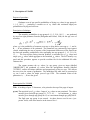
Mean age of childbearing: Mean age of mother at childbearing in the population. This
variable is only used when data are tabulated by age of mother. If data are
tabulated by duration of marriage, this value will not be used.
This variable can be calculated from births tabulated by age of mother at time of
birth as
where B(x-y) is the number of births to women in age group x to y at the time of
birth. An approximate estimate of M can be calculated from children ever born
data through FERTCB or from the age schedule of fertility through FERTPF.
Tabulations: Indicates whether the data are tabulated by age group of mother, or by
duration of her marriage. Since data by age of mother was replaced by QFIVE,
selecting this will give instruction on copying the data to QFIVE.
Children ever born: The average number of children ever born to a woman. If
"Tabulations" above is coded as “age of mother”, the data are given by age groups
(15-20, 20-25, ..., 45-50); if "Tabulations" above is coded as “duration of
marriage”, the data are given by duration of marriage (0-5 years, 5-10 years, ...,
30-35 years).
Children surviving: The average number of children surviving per woman, either by
her age group, or by duration of her marriage.
Sample Input Data
An example data set is given in CEBCS.MPL. In this example, mortality data are
given for a hypothetical population. In this data set, the children ever born and
children surviving are given by age group of mother.
28
D. Description of CENCT
Purpose of procedure
Estimation of completeness of one census relative to a second census from
population age distributions from two censuses, and either assumption of a United
Nations or Coale-Demeny model life table or provision of registered deaths or death rates
by age for the intercensal period.
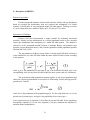
Description of technique
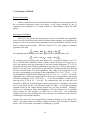
Hill (1987) has shown that in any population closed to migration, the following
equation holds for an intercensal period:
where N(a) and N(a-t) are the number of person years lived at exact age a, and at ages a
and over, respectively, during an intercensal period, r(a+) is the cumulative age-specific
growth rate, D(a+) is registered intercensal deaths for ages a and over, t is the length of
the intercensal period, K is completeness of the second census enumeration relative to the
first, and C is completeness of death registration during the intercensal period. Values of
K and C are assumed to be invariant with age.
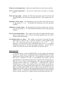
In practice, N(a) and N(a+) are calculated from census population age-sex counts,
as
and
where Pl and P2 refer to the population counts at the first and second census
respectively. The cumulative age-specific growth rate is calculated as
The equation follows directly from Martin's (1980) generalization of the Brass
growth-balance equation. The equation indicates that the ratio of intercensal deaths to the
29
intercensal population is linearly related to a measure easily calculated from two
population censuses. The intercept of the fitted line allows calculations of the coverage of
the second census count relative to that of the first census (K = e It where I is the
intercept). The value of K can therefore be considered a multiplicative adjustment factor.
When applied to the first census, it produces consistency in coverage to the second
census. The computer program estimates the intercept through ordinary least squares
regression. (It should be noted that the value of K, along with the value of the slope,
provides an estimate of the completeness of death registration.)
Intercensal deaths can be provided in either of two ways. As one option, a United
Nations, Coale-Demeny or user-designated model life table, considered appropriate to the
intercensal period, is provided and the computer program estimates intercensal deaths
from the life table central death rates and the two population age distributions. In the
second option, absolute numbers of deaths by age for the intercensal period are given as
input.
Data required for CENCT
Title: A data description of up to 40 characters to be included in the heading at the top
of the page of output.
Deaths:
Indicates the type of mortality data given as input; either deaths are
calculated by a model life table, or deaths are calculated by the given intercensal
deaths by age.
Sex:
Indicates whether the life table refers to the male or female sex.
Final open age group: Indicates the final open age group given for the first and second
populations and for the intercensal deaths. The final open age group must be
between 60+ and 85+.
Model life table pattern:
This variable is used only if "Deaths" are given through a
model life table. It indicates the model life table pattern to be used. The choices
are:
User-defined model
UN Latin American model
UN Chilean
UN South Asian
UN Far East Asian
UN General
Coale-Demeny West
Coale-Demeny North
Coale-Demeny East
Coale-Demeny South
30
If intercensal deaths are generated through a model life table, the life table choice
is indicated by designating a life table column, the age group of interest and the
life table mortality value.
Life table mortality value: This value indicates the mortality value being matched.
The value of m(x,n) or q(x,n) should be between 0 and 1. The value of l(x)
should be based on a radix of 100,000. The value of e(x) is presented in years.
For example, if a model life table is chosen with l(5) = 90000, then the life table
column is set to 3, age is set to 5 and the mortality value is set to 90000.
Life table column:
l(x) or e(x).
The life table column has four choices available: m(x,n), q(x,n),
Life table age: The age group of interest is coded as: 0 = age group 0-1, 1 = 1-5, 5 = 510, 10 = 10-15, ..., 80 = 80-85. When the third life table column is chosen (i.e.,
l(x)), ages 2, 3 or 4 may also be chosen to indicate matching on l(2), l(3) or l(4).
Title for user-defined model: This variable is used only if the model life table pattern
above is coded as zero and "Deaths" above is coded as 1. It is a name for the
model supplied by the user and is included in the table heading.
User-defined model q(x,n) values: This variable is used only if the user indicates the
choice of calculating deaths by “Model Life Table” and the “user-defined” model
life table pattern was chosen. It consists of model q(x,n) values supplied by the
user. The values must be given for age groups 0-1, 1-5, 5-10, … . As a
minimum, q(x,n) values must be given through age group 60-65; as a maximum
through age group 80-85. As these data are read in on a "per-person" basis, each
value must be in the interval 0 to 1.
Month of first enumeration: Indicates the month that the first census was taken.
Year of first enumeration: The year the first census was taken; for example, 1960.
Month of second enumeration: Indicates the month that the second census was taken.
Year of second enumeration:
1970.
The year the second census was taken; for example,
Population of first census: The population by age for the first census. Data are for age
groups 0-5, 5-10, ..., up through the last open given age group available.
Population of second census: The population by age for the second census. Data are
given for age groups 0-5, 5-10, ..., up through the last open age group available.
31
Intercensal deaths: This variable is used only if the user indicates the choice of
calculating deaths by “Intercensal Deaths”. These values are the registered
deaths for the intercensal period. Data are given for age groups 0-5, 5-10, ..., up
through the last open age group available.
Sample Input Data
An example data set is given in CENCT.MPL. In this example, the completeness
of enumeration of the June 1960 census relative to the June 1972 census for a
hypothetical female population is estimated. Mortality data are given as the
absolute number of deaths by age. In conjunction with the population figures
deaths are estimated. The results indicate that the 1972 census is about 5 per cent
less complete than the 1960 census (adjustment factors are around .95) so the
correct population growth rate (between 2.04 per cent and 2.09 per cent) is
slightly higher than the recorded rate (2.0 per cent).
32
E. Description of COMBIN
Purpose of procedure
Calculates a "model" life table from an estimate of life expectancy at age 20 or
q(15,n) combined with an estimate of survivorship to age 1, survivorship to age 5, or both
(can be substituted with 1qo and 5q0).
Description of technique
The procedure adjusts a designated United Nations or Coale and Demeny model
life table to incorporate the child and adult survivorship values given as input. Agespecific probabilities of dying (q(x,n) values) consistent with these survivorship values
are determined separately for ages 20 and over and for ages under 20. For ages 20 and
over, q(x,5) values from the designated model life table pattern and life expectancy at age
20 are accepted. These q(x,5) values are calculated through the procedure MATCH.
The method of calculating age-specific mortality rates under age 20 depends upon
the form of the input data. In the "complete" case, survivorship to both age 1 (i.e. l(1))
and age 5 (i.e., l(5)) are given, allowing straightforward calculation of q(0,1) and q(1,4).
Given q(0,1) and the value of q(20,5) calculated above, the procedure BESTFT is called
to provide interpolated values of q(5,5), q(10,5) and q(15,5) (based on the second
component fit to the designated model). Next, q(1,4) and q(20,5) are used in an identical
way to provide a second set of interpolated values of q(5,5), q(10,5) and q(15,5). The
average of these two sets of values is accepted. If only l(5) is given, then procedure
MATCH is used to calculate q(0,1) and q(1,4) values which are consistent with the l(5)
value and the designated model. Then, q(5,5), q(10,5) and q(15,5) are calculated as
mentioned previously. If only l(1) is given. the procedure BESTFT is used to calculate
interpolated values for q(1,4), q(5,5) q(10,5) and q(15,5), given q(0,1) and q(20,5).
Starting with version 4.3, the values of q(0,1) and q(0,5) can be substituted for l(1) and
l(5). The value of q(15,n) can be inputted instead of e(20), where “n” can be any valid
value selected as input (default 5 when zero or blank). The value of “n” is valid when
“x+n” has a value of 1, 5, 10, 15, 20, …, up to the open age group.
With the complete set of q(x,n) values the procedure LIFTB is used to print the
output table.
Data required for COMBIN
Title: A data description of up to 72 characters, to be printed at the top of the page of
output.
33
Model life table pattern: Indicates the model life table pattern to be used. The choices
are:
United Nations Latin American
United Nations Chilean
United Nations South Asian
United Nations Far East Asian
United Nations General
Coale-Demeny West
Coale-Demeny North
Coale-Demeny East
Coale-Demeny South
Sex:
Indicates whether the male or female population is being considered.
e(20): Life expectancy at age 20 in the population under study.
l(1):
The probability of surviving to age 1 (times 100,000) in the population under
study.
l(5):
The probability of surviving to age 5 (times 100,000) in the population under
study.
Help notes
Either l(1) or l(5) or both must be entered, but both cannot be left blank. They
can be calculated as follows:
l(1) = 100000 * [ 1 – q(0,1) ]
l(5) = 100000 * [ 1 – q(0,1) ] * [ 1 – q(1,4) ]
Sample Input Data
An example data set is given in COMBIN.MPL. In this example, data are given
for a hypothetical population with a life expectancy at age 20 of 50 years. In this
data set, the Latin American pattern is combined with a value of l5 of 78000 and a
value of l1 of 85000.
34
F. Description of COMPAR
Purpose of procedure
Compares empirical set of age-specific central death rates (m(x,n) values) or agespecific probabilities of dying (q(x,n) values) to all United Nations and Coale-Demeny
model life table patterns and prints out indices of similarity. The q(x,n) values can be
substituted with l(x) values as input.
Description of technique
For each age-specific m(x,n) or q(x,n) value given as input (for age groups 0-1, 15, 5-10, 10-15, ...), the corresponding life expectancy at birth in each of the five United
Nations models and four Coale-Demeny models is found (by calling the procedure
MATCH) and printed out. For each model, a series of life expectancies which are more
or less constant by age indicates that the empirical mortality pattern is similar to that
model. Indices of goodness of fit for age groups 0 to 10, 10 and over, and 0 and over are
calculated and printed by the COMPAR procedure. The first index used is
where a and b indicate the lower and upper age groups being considered, E(x,n) indicates
the life expectancy at birth in the model which corresponds to the mortality rate in age
group (x, x+n), M indicates the median of the E(x,n) within the range (a, b), and N is the
number of age groups within the range. Indices are printed out for age ranges 0 to 10, 10
and over, and 0 and over. The second index printed out is the difference between the
median within the age range 0 to 10 and the median within the age range 10 and over. In
all cases the lower the value of the index, the better the fit to the model.
Special comments
The output is limited to age group 75-80 because Coale-Demeny tables are
limited to 80+.
Data required for COMPAR
Title: A data description of up to 72 characters, to be included in the heading at the top
of the page of output.
Sex:
Indicates whether the m(x,n) or q(x,n) values refer to the male or female sex.
35
Type of mortality data:
Indicates whether q(x,n), m(x,n) or l(x) values are being
given as input. This selection is used to describe the age-specific mortality data.
Changing the data type will not convert the age-specific mortality data from one
type to another.
Age-specific mortality data: The age-specific mortality data themselves. No matter
whether q(x,n) or m(x,n) values are used as input, the values are input in the same
way. For ages 5 and over the values must be given for five year age groups. For
ages under 5 they are given for age groups 0-1 and 1-5. As these data are read in
on a "per-person" basis, each value must be in the interval 0 to 1. Mortality data
must be entered for all ages through age group 60-65. The maximum age group
permitted is 75-80. Remember that the final open age group is not entered; the
m(n+) or q(n+) value for the last age group is not used by the COMPAR
procedure. Starting with version 4.3, q(x,n) values can be substituted with l(x)
values.
Sample Input Data
An example data set is given in COMPAR.MPL. In this example, a set of q(x,n)
values for a hypothetical female population is read in. Data are supplied for age
groups 0-1, 1-5, 5-10, …, up to 75-80. The empirical data are shown, by the
output, to be most similar to that of the Coale-Demeny North region. This was
determined by observing that its average deviation from the median for all age
groups is 1.9, the lowest value of all regions. However, if only the childhood ages
are under consideration (ages 0 to 10), then the United Nations General Pattern is
better, with an average deviation of only 0.4.
36
G. Description of CORMOR
Purpose of procedure
Display corresponding probabilities of dying for selected age groups.
Description of technique
This application was added to version 4.3 of MORTPAK and displays “Corresponding
Mortality Indicators”. Each row corresponds to probabilities of dying for various preselected age groups. Column headers are for the 9 model life table regions. The input
data is similar to MATCH and is used to set the level of each model of the model life
tables. The corresponding mortality values are calculated and displayed in the output
table.
Data required for CORMOR
Title: A data description of up to 72 characters, to be included in the heading at the top
of the page of output.
Sex: Indicates whether the life table refers to the male sex or female sex.
Life table mortality value: This value indicates the mortality value being matched. For
example, if a model life table is chosen with l(5) = 90000, then the mortality value
is set to 90000.
Life table column: The life table columns are m(x,n), q(x,n), l(x) or e(x).
Life table age: The l(x) or e(x) columns are for exact age x. The m(x,n) or q(x,n)
columns are for age groups age x to x+n. The default age group of interest is
entered as: 0 = age group 0-1, 1 = 1-5, 5 = 5-10, 10 = 10-15, …, 80 = 80-85.
When the third life table column is chosen (i.e., l(x)), ages 2, 3 or 4 may also be
chosen to indicate matching on l(2), l(3) or l(4). The other columns may not use
ages 2, 3 or 4.
Life table age group interval: When inputting m(x,n) or q(x,n), the value of “n” may be
entered as input. In previous versions of MORTPAK, the value of “n” was the
interval from the current to the next age group and is now considered the default
value. The default value is used whenever “n” is not supplied or has a value of
zero.
37
H. Description of FERTCB
Purpose of procedure
Estimation of age-specific fertility rates from data on children ever born tabulated
by age of mother recorded at either one or, optionally, two points in time.
Description of technique
Arriaga (1983) has shown how age-specific fertility rates can be calculated from
recorded data on children ever born by age of woman.
The method is best used in situations when children ever born data are available at
two points in time. The approach of Arr:iaga is (i) to obtain average number of children
ever born for women exact age x at the time of the first and second enumeration
[CEBx(t1) and CEBx(t2)] through graduation by a ninth degree polynomial, on the data on
children ever born in five-year age groups recorded in each enumeration; (ii) to estimate
children ever born at exact age x for the year after the first census [CEBx(t1+1)] and the
year before the second census [CEBx(t2-1)] by linear interpolation between CEBx(tl) and
CEBx(t2) for every age x; (iii) to calculate single-year age-specific fertility rates for the
one-year period following the first census as fx1 = CEBx+1(tl+1) -CEBx(t1) and for the
one-year period preceding the second census as fx2 = CEBx+1(t2) -CEBx(t2-1) ; (iv) to
ensure that the age-specific fertility rates at older ages decrease monotonically and
exponentially to zero at age 50, adjust the estimated single-year age-specific fertility rates
at ages 40 and over by assuming that fxi = f39 + (1 – f39)(x-39)/11 – 1; and, finally, (v) to
calculate age-specific fertility rates in conventional five-year age groups for each time
period by taking the arithmetic average of the single-year age-specific fertility rates
within each five-year age group.
When children ever born data are only available at one point of time, the method
can still be applied, although only under the case of constant fertility (Mortara, 1949).
Simply,
fx = CEBx+l - CEBx
where fx is the fertility rate for women in age group (x, x+l) and CEBx is the recorded
average number of children ever born for women exact age x. Graduation is necessary to
estimate average numbers of children ever born for women at exact age x from the usual
recorded data on average numbers of children ever born in five-year age groups (x, x+5).
Arriaga (1983) uses a ninth-degree polynomial for this graduation; he also outlines the
steps for calculation of fertility rates for conventional five-year age groups from the
single-year fx values (see steps (iv) and (v) in the previous paragraph).
38
The procedure also generates an estimate of the mean age of mother at
childbearing in the population. The mean age is calculated based on the estimated agespecific fertility rates and the 1985 age distribution of the female population for all less
developed countries combined according to the United Nations medium variant
projections.
Data required for FERTCB
Title: A data description of up to 72 characters, to be included in the heading at the top
of the page of output.
Month of first enumeration: Indicates the month of the first enumeration.
Year of first enumeration: The year of the first enumeration.
Month of second enumeration: Indicates the month of the second enumeration. Leave
blank if data from only one enumeration are being entered.
Year of second enumeration: The year of the second enumeration. Leave blank if data
from only one enumeration are being entered. When blank or zero, the procedure
assumes that the second enumeration is not available. Therefore, any data given
for the second enumeration is ignored.
Children ever born (first enumeration) The average number of children ever born
per woman at the time of the first enumeration. Data are given for age groups 1520, 20-25, ..., 45-50.
Children ever born (second enumeration) The average number of children ever born
per woman at the time of the second enumeration. Data are given for age groups
15-20, 20-25, ..., 45-50. These fields are left blank if data from only one
enumeration are being entered. If the year of the second census is blank or zero,
the procedure assumes that the second enumeration is not available. Therefore,
any data given for the second enumeration is ignored.
Sample Input Data
An example data set is given in FERTCB.MPL. In this example, data on children
ever born in five-year age groups are available for a hypothetical population from
enumerations during July 1970 and May 1976. The Arriaga approach is used to
estimate age-specific fertility rates for July 1970 – July 1971 and May 1975 –
May 1976.
39
I. Description of FERTPF
Purpose of procedure
Estimation of age-specific fertility rates from data on children ever born tabulated
by age of mother and the age pattern of fertility, recorded at either one or, optionally, two
points in time.
Description of technique
Recorded age-specific fertility rates often underestimate the true level of fertility
owing to omission of events from civil registration systems or surveys or
misunderstanding of the length of the reference period in survey questions on births
during a previous period. Because of reference period errors, age specific fertility rates
calculated from surveys are also occasionally overestimated. Brass (Brass and others,
1968) developed a method, commonly known as the P/F method, for evaluating and
adjusting these recorded fertility rates by comparing the recorded rates to data on average
number of children ever born tabulated by five-year age group of woman. The P/F
approach assumes that fertility has been constant in the past, that the pattern (although, of
course, not the level) of the recorded age-specific fertility rates (denoted ASFP) is
correct, and that the level of lifetime fertility for the younger cohorts of women provided
by the children ever born data (CEB) are correct. Brass simply cumulated and graduated
the recorded ASFP data to be in the form of children ever born data. Under the
assumption of constant fertility, these transformed data (denoted nFx) are comparable to
the recorded children ever born data (nCEBx). The ratios of nCEBx/nFx for the younger
age groups provide possible adjustment factors to be applied to the recorded fertility
rates.
Arriaga (1983) later modified the method and extended it to the case of changing
fertility. Rather than transforming the recorded ASFP figures to CEB-type figures, he
suggested transforming the recorded CEB data into estimates of age-specific fertility (by
the method outlined in the program FERTCB). These two sets of age-specific fertility
rates are then cumulated by age, and the ratios of these cumulated figures provided
possible adjustment factors. According to Arriaga (1983, pp. 3-8), this modification not
only has analytical and diagnostic advantages but also leads to extension of the method to
conditions of changing fertility. If the children ever born (CEB) and fertility pattern data
(ASFP) are available from two enumerations, age-specific fertility rates can be estimated
for the one-year period following the first enumeration and the one-year period preceding
the second enumeration, by the method described in FERTCB. The estimated agespecific fertility rates can then be compared to the recorded ASFP data to provide
adjustment factors in the same way as is done for the constant fertility (one set of data)
approach.
The procedure also generates an estimate of the mean age of mother at
childbearing in the population. The mean age is calculated based on the estimated age-
40
specific fertility rates and the 1985 age distribution of the female population for all less
developed countries combined according to the United Nations medium variant
projections.
A full description of the Brass and Arriaga approaches for estimating age-specific
fertility rates from recorded children ever born data and the age pattern of fertility is
given in Arriaga (1983).
Data required for FERTPF
Title: A data description of up to 72 characters to be included in the heading at the top
of the page of output.
Month of first enumeration: Indicates the month of the first enumeration.
Year of first enumeration: The year of the first enumeration.
Fertility pattern of first enumeration: Indicates how the fertility pattern from the first
enumeration is tabulated; whether by age of mother at time of birth of the child or
by age of mother at the date of enumeration.
Children ever born (first enumeration): The average number of children ever born
per woman at the time of the first enumeration. Data are given for age groups 1520, 20-25, …, 45-50.
Age-specific fertility pattern (first enumeration): The age-specific fertility pattern at
the time of the first enumeration. Data may be given as recorded age-specific
fertility rates or as the proportionate age distribution of fertility. Data are given for
age groups 15-20, 20-25, ..., 45-50.
Month of second enumeration: Indicates the month of the second enumeration. Leave
blank if data from only one enumeration are being entered.
Year of second Enumeration: The year of the second enumeration. Leave blank if data
from only one enumeration are being entered.
Fertility pattern of second enumeration: Indicates how the fertility pattern from the
second enumeration is tabulated; whether by age of mother at time of birth of the
child or by age of mother at the date of enumeration
Children ever born (second enumeration): The average number of children ever born
per woman at the time of the second enumeration. Data are given for age groups
15-20, 20-25, ..., 45-50. Leave blank if data from only one enumeration are being
entered.
41
Age-specific fertility pattern(second enumeration): The age-specific fertility pattern
at the time of the second enumeration. Data may be given as recorded agespecific fertility rates or as the proportionate age distribution of fertility. Data are
given for age groups 15-20, 20-25, ..., 45-50.
Help notes
Data can be given for one or two periods of time. If the year of the second census
is blank or zero, the procedure assumes that the second enumeration is not
available. Therefore, any data given for the second enumeration are not used.
It doesn’t matter whether the fertility pattern is entered as age-specific fertility
rates or as a proportional distribution. The figures are adjusted by the multipliers
to give identical results.
Sample Input Data
An example data set is given in FERTPF.MPL. In this example, data on children
ever born and recorded fertility rates in five-year age groups are available for a
hypothetical population from an enumeration of July 1970. The Arriage/Brass
approach is used to adjust the recorded age-specific fertility rates to provide
“corrected” fertility estimates fro July 1970. The recorded age-specific fertility
rates were tabulated by age of mother at the time of the birth of the child. The
results imply that the recorded fertility underestimated actual fertility by about 14
per cent and the true total fertility rate is about 6.7 births per woman.
42
J. Description of ICM
Purpose of procedure
Estimates single-year probabilities of dying (lqx values) for ages under 5 from
probabilities of dying in age groups 0-1, 1-5 and 5-10.
Description of technique
Estimates of single-year mortality under age 5 are generated using the three-parameter
interpolation formula
ln(-ln lqx) = ln(-ln tl) + t3 * ln (x + t2)
where x is the age and t1, t2 and t3 are chosen so that the interpolation equation is
consistent with given values of 1q0, 4ql and 5q5.
The equation was chosen after observation that, in a wide range of countries, ln(-ln 1qx)
values were linearly related to ln(x) for ages 1 through 7 or 8 years. The addition of the
parameter t2 brought infant mortality in line with the linear relationship (Heligman and
Pollard, 1980). Probabilities of dying (lqx) by single years of age for ages under 5 are
presented along with the corresponding number of survivors at each age (lx).
Data required for ICM
Title: A heading of up to 72 characters, to be printed at the top of the page of output.
The empirical set of nqx values, for age groups 0-1, 1-5 and 5-10. As these
data are read in on a "per-person" basis, each value must be in the interval 0 to 1.
q(x,n):
Sample Input Data
An example data set is given in ICM.MPL. In this example, probabilities of
dying (nqx values) for ages 0-1, 1-5 and 5-10 are given as input and interpolated
1qx values and corresponding lx values for ages 0, 1, 2, 3 and 4 are calculated and
printed.
43
K. Description of LIFTB
Purpose of procedure
Construction of a life table based on a set of age-specific central death rates (nmx
values), age-specific probabilities of dying (nqx values) or number of survivors at age x (lx
values).
Description of technique
Based on a given set of nmx or nqx values for age groups 0-1, 1-5, 5-10, ..., up to
the last closed age group available (maximum of 95-100 is allowed; value for the final
open age group is not given), an abridged life table is constructed. Starting with
MORTPAK 4, lx values for ages 0, 1, 5, …, up to a maximum age of 100 may now be
entered. The usual life table columns are calculated, labeled on the computer output and
defined, as follows:
Age:
the initial age of the age interval (x, x+n) where x is the initial age and n is
the length of the interval. The interval length is five years, with the
exception of infancy (one year), early childhood years (four-year age
group) and last interval (open ended);
m(x,n):
central death rate for the age interval (x, x+n). Usual notation is nmx;
q(x,n):
probability of an individual age x dying before the end of the age interval
(x, x+n). Usual notation is nqx;
l(x):
number of survivors at age x in a life table with radix (starting population)
of 100,000 persons. Usual notation is lx;
d(x,n):
number of deaths in age interval (x, x+n). Usual notation is ndx;
L(x,n):
number of person-years lived in age interval (x, x+n). Usual notation is
nLx;
S(x,n):
the proportion of the life table population in age group (x, x+n) who are
alive n year later. Usual notation is nSx;
T(x):
number of person-years lived at ages x and older. Usual notation is Tx;
e(x):
expectation of life at age x. Usual notation is ex;
a(x,n):
average number of years lived in the age interval (x, x+n) by those dying
during that age interval. Usual notation is nax.
44
The procedure for constructing the life table from the nmx or nqx values is based on
a method developed by Greville (1943). To complete the life table the nqx values are
extrapolated until no survivors remain, by fitting a Makeham function through the last six
nqx / (l - nqx) values available (United Nations, 1982, p. 31).
Data required for LIFTB
Title: A heading of up to 72 characters, to be printed above the calculated life table.
Sex: Indicates whether the life table refers to the male or female sex. This variable is
used for calculating the first two separation factors (la0 and 4al).
Type of mortality data: Indicates whether nqx, nmx or lx values are being given as
input. This selection is used to describe the age-specific mortality data.
Changing the data type will not convert the age-specific mortality data from one
type to another.
(Output) open age group: This open age group refers to the output table only. The
open age group for the input is still determined from the last entry of the agespecific mortality data. The default value is “same as input” where the input and
output use the same open age group and is consistent with earlier versions of
MORTPAK. The output open age group can have a value ranging from 60+
through 100+. When the output is smaller than the input, the output table will be
compressed. When the output is larger than the input, the output table will be
extrapolated. Large extrapolations should be done with caution. Check the
output thoroughly.
Age-specific mortality data: The age-specific mortality data themselves. No matter
whether nqx or nmx values are used as input, the values are input in the same way.
For ages 5 and over the values must be given for five-year age groups. For ages
under 5 they are given for age groups 0-1 and 1-5. As these data are read in on a
"per-person" basis, each value must be in the interval 0 to 1. If lx values are given
as input, the values must be based on a radix (l0) of 100,000. Values must be
given for all ages 0, 1, 5, 10 ,15, …, 65, with a maximum of age 100. Mortality
data must be entered for all ages through age group 60-65. The maximum age
group permitted is 95-100. Remember that the final open age group is not
entered; the m(n+) or q(n+) value for the last age group is calculated by the
LIFTB procedure.
45
Sample Input Data
An example data set is given in LIFTB.MPL. In this example, a set of mortality
data for a hypothetical female population is processed and a life table constructed
and printed. Mortality probabilities, i.e., nqx values, are given for age groups up to
75-80.
46
L. Description of MATCH
Purpose of procedure
Calculates and prints out United Nations, Coale-Demeny or user-designated
model life tables corresponding to given levels of mortality. As the user-designated
model can be a mortality pattern specific to a certain population, MATCH can generate a
country-specific model life table system.
Description of technique
The user must designate the model pattern (any of the five United Nations, four
Coale-Demeny patterns or an external model supplied by the user) and the sex desired.
The United Nations principal component equations (United Nations, 1982, p. 8) or CoaleDemeny regression equations (Coale-Demeny, 1966, p. (21)) are then used with an
iterative procedure to find the model corresponding to a given level of mortality. The
iterative procedure is described in United Nations, 1982 (pp. 22-23). However, because
of potential extrapolation problems, model life tables are calculated only when life
expectancy at birth is between 20 and 80 years. When a user-defined pattern is used, it is
permitted to go up to 90 years. The mortality level is specified by the user by designating
a mortality value for one of four life table functions (nmx, nqx, lx or ex) for any one of the
age groups. The iterative procedure is carried out by the procedure MATCH, which calls
the procedures LIFTB and, when necessary, ICM for construction of the model life table
itself. The model life table is presented as computer output; the life table columns are as
given in the description of the procedure LIFTB. Starting with 4.3, while this application
still contains the traditional (i.e. unchanged) model life tables from previous versions,
new enhanced life tables were added. The new model life tables have age patterns which
were updated and have been expanded to include life expectancies at birth to age 100.
When matching on q(x,n) or m(x,n), the value of "n" can now be selected as input. If
“n” is zero or blank, its value will default to the interval between the current and next age
group.
Data required for MATCH
Title: A data description of up to 40 characters, to be included in the heading at the top
of the page of output.
Model life table pattern: Indicates the model life table pattern to be used. The choices
are:
User-defined model
United Nations Latin American model
United Nations Chilean
United Nations South Asian
47
United Nations Far East Asian
United Nations General
Coale-Demeny West
Coale-Demeny North
Coale-Demeny East
Coale-Demeny South
If the user-defined model is chosen, the user is supplying the average pattern of
mortality to be used as a model (see "User-Defined Model nqx values" below).
The United Nations principal component equations are then used to adjust this
pattern to the desired mortality level.
Sex:
Indicates whether the life table refers to the male or female sex.
The life table choice is indicated by designating a life table column, the age group of
interest and the life table mortality value.
Life table mortality value: This value indicates the mortality value being matched. For
example, if a model life table is chosen with l5 = 90000, then the mortality value
is set to 90000.
Life table column: The life table columns are nmx, nqx, lx or ex.
Life table age: The lx or ex columns are for exact age x. The nmx or nqx columns are
for age groups; therefore, the age group of interest is entered as: 0 = age group 01, 1 = 1-5, 5 = 5-10, 10 = 10-15, …, 80 = 80-85. When the third life table column
is chosen (i.e., lx), ages 2, 3 or 4 may also be chosen to indicate matching on l2, l3
or l4. The other columns may not use ages 2, 3 or 4. Starting with 4.3, if the new
models are chosen and q(x,n) or m(x,n) is selected, then the value of “n” may be
set to any valid value. A blank or zero value will be set to the default value.
Value of final life table and increment between life tables: When a series of model
life tables are desired, values for the final life table and the increment between
tables must also be given. A maximum of 50 tables can be requested through this
option. For example, if a series of model life tables is desired in which e5 varies
from 40 to 60 years at five-year intervals, we would choose life table column as
e(x), the age as 5, the model life table mortality value as 40.0, the final mortality
value as 60.0 and the increment as 5.0.
Label for user-defined model: This variable is used only if the model life table pattern
chosen is “User-defined model”. It is a name for the model supplied by the user and is
included in the table heading.
User-defined model nqx values: This variable is used only if the model life table
pattern chosen is “User-defined model”. It consists of model nqx values supplied
by the user. The values must be given for age groups 0-1, 1-5, 5-10, … . As a
48
minimum, nqx values must be given through age group 60-65; as a maximum
through age group 80-85. As these data are read in on a "per-person" basis, each
value must be in the interval 0 to 1.
Help Note
When a series of model life tables is selected by giving a final life table value and
an increment between life tables, a combo box is created on the worksheet with
the label “SELECT TABLE TO SHOW”. Clicking the cell with the combo box
will display a drop down list containing an entry for each available life table.
These life tables are created and updated whenever “Run” is selected. If the input
data is updated, it is necessary to “Run” the application to update the output life
tables.
Sample Input Data
An example data set is given in MATCH.MPL. In this example, a user-defined
model life table is calculated. A set of nqx values supplied by the user based on a
neighboring country is given, and the first component vector of the United
Nations models is used to adjust them to correspond to a life expectancy at birth
of 65 years.
49
M. Description of ORPHAN
Purpose of procedure
To estimate female adult mortality from tabulations on proportion of population
with mothers still alive by age group of respondents.
Description of technique
Brass and Hill (1973) have shown that the proportion of population with mother
still alive can be used to generate estimates of adult female mortality. Hill and Trussell
(1977) later proposed an estimation equation of the form
nl25
= a(n) + b(n) AGE + c(n) 5Sn-5
where nl25 is the life table probability of female survival from age 25 to age 25+n, AGE is
the mean age of childbearing for women in the population, 5Sn-5 is the proportion of the
population in age group (n-5, n) with mother still alive, and a(n), b(n) and c(n) are agespecific constants (presented by Hill and Trussell in tabular form). (An approximate
estimate of AGE is produced by the procedures FERTCB and FERTPF.) In practice,
only values of n varying from 20 to 50 are used, corresponding to age groups of
respondents 15-20, 20-25, 25-30, ..., 45-50 and probabilities of female survival from age
25 to 45, 25 to 50, ..., 25 to 75. The constants a(n), b(n) and c(n) were estimated by Hill
and Trussell through regression procedures on simulated data which were in turn based
on the Coale-Demeny model life tables. Palloni and Heligman (1985), using the identical
formulations, later presented revised constants based on each of the five patterns
underlying the United Nations models. In sum, then, a choice of six sets of estimating
equations are available, one based on the Coale and Demeny models and five based on
the United Nations models. Through a second set of simulations, Palloni and Heligman
also developed a set of regression equations which estimate the time reference to which
the nl25 values refer. These regression equations are based on the United Nations General
Pattern of mortality but appear to apply equally well to all of the United Nations patterns,
as well as the Coale and Demeny based pattern. The independent variables, which are
calculated from the input data, necessary for calculating these time references are: the
ratio of average number of children ever born for women in age group 15-20 to that in
age group 20-25, the ratio of average number of children ever born for women in age
group 20-25 to that in age group 25-30, and the average age of childbearing among
women in the population. Starting with 4.3, new output tables were added to display
q(15,45) and q(15,35). An output column was added to display reference dates in
numeric "decimal" format. This is convenient, for example, if displaying x/y graphs.
50
Data required for ORPHAN
Title: A data description of up to 72 characters, to be to be included in the heading at the
top of the page of output.
Month: Indicates the month of the enumeration.
Year: The year of the enumeration; for example, 1970.
Age:
The mean age of mother at childbearing in the population.
Proportion with mother alive: The proportion of population with mother still alive.
Data are given for age groups 15-20, 20-25, ..., up to 45-50.
Children ever born: The average number of children ever born to a woman. Data are
given for age groups 15-20, 20-25 and 25-30. Only the first three age groups
from the children ever born tabulations are required. The other four age groups
are not used and are not entered.
Help Note
The mean age of mother at childbearing (M) in the population can be calculated
from births tabulated by age of mother at time of birth as
where B(x-y) is the number of births to women in age group x to y at the time of birth.
An approximate estimate of M can be calculated from children ever born data through
FERTCB or through FERTPF.
Sample Input Data
An example data set is given in ORPHAN.MPL. In this example, estimates of
adult female mortality and corresponding life expectancies for a hypothetical population
are calculated and printed. The average age at childbearing is 26.00 and the proportion of
the population with mother still alive is given for age groups 15-20, 20-25, …, up to 4550. To calculate the reference dates, the average number of children ever born for age
groups 15-20, 20-25 and 25-30 are given.
51
N. Description of PRESTO
Purpose of procedure
Provides integrated estimates of intercensal mortality, fertility and age distribution
based on recorded age distributions from two censuses and assumption of a United
Nations, Coale-Demeny or user-designated model life table pattern. Starting in version
4.3, new output tables were added to display q(15,45) and q(15,35) values.
Description of technique
Preston (1983) has demonstrated a simple method for estimating intercensal
mortality, fertility and age distributions in a closed population based on two recorded
census age distributions and assumption of a model life table pattern. The method is
referred to as the "integrated method" because it combines Brass's one-parameter logit
mortality system (Brass and others, 1968) with the generalized stable population equation
(Preston and Coale, 1982).
The one-parameter (α) Brass system relates a chosen model life table (referred to
as the standard) to any other life table within the same model life table system according
to the equation
where ps(a) is the probability of surviving to age a in the model life table, p(a) is the
corresponding value for any other life table within the same system, and α is a parameter.
The generalized stable population equation applies to any closed population and
relates the current age distribution to current levels of mortality, fertility and age-specific
growth rates. Namely,
where c(a) is the proportion of the population aged a, b is the crude birth rate, r(x) is the
growth rate of persons age x, and p(a) is the probability of survival to age a.
If we assume that p(a) in equation (1) describes the current life table for the population
described by equation (2), we can solve equation (1) for p(a), substitute into equation (2)
and after further manipulation,
52
As estimates of p(5), the probability of surviving to age 5, are generally available
from children ever born/children surviving tabulations (see CEBCS), the above equation
can be refined as
where a≥5 and 5ps(a) indicates that the radix of the life table is unity at age 5. The
variable on the left-hand side of equation (3) can be estimated, on an intercensal basis,
from the age distributions in two censuses. With choice of life table from a model life
table pattern (either a United Nations, Coale-Demeny or user-designated pattern)
appropriate to the country under study, the quantity in brackets on the right-hand side can
be calculated and the left-hand side of equation (3) can be regressed on the right-hand
side. The regression minimizes the sum of squared relative differences between observed
and predicted values. The estimated regression parameters provide estimates of the
demographic parameters during the intercensal period: the reciprocal of the intercept
equals the crude birth rate and eα adjusts the chosen model life table to the correct level.
From introduction of the estimated intercensal birth rate (b) and survival function [p(a)]
into equation (2), the "correct" intercensal age distribution is obtained. This correct
intercensal age distribution can be compared with an average of the recorded age
distribution for an analysis of errors in age recording in the censuses.
The required input is therefore the population age distributions from two
censuses, a model life table to be used as the standard, and estimates of survivorship to
age 5 and age 1 for the intercensal period. The last datum permits refined calculation of a
life table beginning at age 0; it does not affect calculated crude birth rates, life expectancy
at age 5 or the estimated intercensal age distribution. Up to nine regressions are
calculated (depending on the number of age groups available), providing nine separate
sets of estimates. The regressions vary according to the range of ages used; the initial age
is 5, 10 or 15 and the terminal age is 60, 65 or 70.
For more information about this technique, see Preston (1983).
Data required for PRESTO
Title: A data description of up to 40 characters, to be included in the heading at the top
of the page of output.
53
Model life table pattern: Indicates the model life table pattern to be used. The choices
are:
User-defined model
United Nations Latin American model
United Nations Chilean
United Nations South Asian
United Nations Far East Asian
United Nations General
Coale-Demeny West
Coale-Demeny North
Coale-Demeny East
Coale-Demeny South
If a user defined model is selected, the user is supplying the average pattern of
mortality to be used as a model (see "User-Defined Model" below).
Sex:
Indicates whether the life table refers to the male or female sex.
The life table choice is indicated by designating a life table column, the age group of
interest and the life table mortality value.
Life table mortality value: This value indicates the mortality value being matched. For
example, if a model life table is chosen with l5 = 90000, then the life table column
is set to 3, age is set to 5 and the mortality value is set to 90000.
Life table column: The life table columns are nmx, nqx, lx, or ex.
Life table age: The lx or ex columns are for exact age x. The nmx or nqx columns are
for age groups; therefore, the age group of interest is entered as: 0 = age group 01, 1 = 1-5, 5 = 5-10, 10 = 10-15, …, 80 = 80-85. When the third life table column
is chosen (i.e., lx), ages 2, 3 or 4 may also be chosen to indicate matching on l2, l3
or l4. The other columns may not use ages 2, 3 or 4.
Probability of surviving from birth to age 1: Probability of surviving from birth to
age 1 in the country being studied. Its purpose is to allow the printing of a life
table beginning with age 0. It can be calculated as l1=100000*(1-1q0).
Probability of surviving from birth to age 5: Probability of surviving from birth to
age 5 in the country being studied. It can be calculated as l5=100000*(1-1q0)* (14q1).
Month of first enumeration: Indicates the month that the first census was taken.
Year of first enumeration: The year the first census was taken; for example, 1970.
54
Month of second enumeration: Indicates the month that the second census was taken.
Year of second enumeration:
1970.
The year the second census was taken; for example,
Final open age group: Indicates the final open age groups given for the first end
second population. The final open age group must have a value ranging from 65+
to 85+.
Population of first census: The population by age for the first census. Data are given
for age groups 0-5, 5-10, ..., up through and including the last open age group
available.
Population of second census: The population by age for the second census. Data are
given for age groups 0-5, 5-10, up through and including the last open age group
available.
Title for user-defined model: This variable is used only if the model life table pattern
above is coded as zero. It is a name for the model supplied by the user and is
included in the table heading.
User-defined model nqx values: This variable is used only if the model life table
pattern above is coded as zero. It consists of model nqx values supplied by the
user. The values must be given for age groups 0-1, 1-5, 5-10, … . As a
minimum, nqx values must be given through age group 60-65; as a maximum
through age group 80-85. The open age group is not given. As these data are
read in on a "per-person" basis, each value must be in the interval 0 to 1.
Sample Input Data
An example data set is given in PRESTO.MPL. In this example, the integrated
procedure is carried out for a hypothetical female population based on census
enumerations of June 1960 and June 1970. The age pattern of mortality for the
adult years is assumed to be that of Coale-Demeny north region, with the
approximated level of mortality assumed to be consistent with a life expectancy at
birth of 50 years. Based on external analyses, early age survivorship has been
determined to have values of l1 = 90,000 and l5 = 85,000 based on a radix of
100,000 persons at birth. Nine regressions have been carried out and all give
similar results since all data points seem to appear on a fairly straight line (see
figure in sample output) indicate that the fit based on age group 10-60 may be
slightly better than the others and the demographic parameters for that regression
should be chosen. Comparison of the adjusted and enumerated censuses indicate
that the recorded censuses have a slightly younger age distribution than the true.
55
O. Description of PROJCT
Purpose of procedure
Projects annually a population by age and sex for up to 100 years, based on the
initial population (by five-year age groups and sex) and an assumption of future changes
in fertility, mortality and migration.
Description of technique
The procedure carries out a single-year projection of a population by age and sex,
based on initial male and female populations in five-year age groups and assumed
changes in fertility and mortality. Projections can be made for up to 100 years. The
methodology used is cohort-component (see Shryock and Siegel, 1973). The steps are
(1) estimation of projected levels and age patterns of mortality, fertility and migration for
each single-year projection period; (2) estimation of the male and female populations by
single years of age from the data in five-year age groups given as input; (3) sequential
application of these annual age-specific mortality and fertility rates and migration to the
population to provide annual projected populations by age and sex and demographic
indicators.
Step 1. Life expectancy at birth for males and for females must be given as input
for the initial and final projection years; life expectancy values for intermediate
projection years are given at the option of the user. Life expectancy at birth for omitted
years is calculated by linear interpolation with respect to year. The age pattern of
mortality is provided as a United Nations model, Coale-Demeny model, or userdesignated (empirical) life table. These models have been extended to life expectancies
at birth of 92.5 years for males and females based on the ultimate life tables prepared by
the United Nations Population Division (see United Nations, 1989b, p. 19).
The
procedure UNABR is used to calculate single-year probabilities of dying [ 1qx ] for every
projection year from those in the standard age groups (0-1, 1-5, 5-10, 10-15, ...). With
these [ 1qx ] values, single-year survival ratios [ 1Sx ] and survivors to age a [p(a)] can be
calculated for each projection year.
Like life expectancy, total fertility rates (TFR) must be given as input for the
initial and final projection years; TFR values for intermediate projection years are given
at the option of the user. The TFR for omitted years is calculated by linear interpolation.
Age-specific fertility rates (ASFR) are provided for the initial and final projection years.
The age-specific fertility rates for intermediate years are calculated by linear interpolation
with respect to corresponding values of the TFR.
Like life expectancy, migration for males and females must be given as input for
the initial and final projection years; migration values for intermediate projection years
56
are given at the option of the user. The migration for omitted years is calculated by linear
interpolation.
Step 2. Initial male and female populations are provided in five-year age groups.
In order to carry out single-year population projections, data are needed in single-year
age groups. Population by single years of age are interpolated using Beers multipliers
(see Beers, 1945).
Data required for PROJCT
Title: A data description of up to 40 characters, to be included in the heading at the top
of the page of output.
Year of base population: Indicates the year for the starting date of the projection; for
example, 1985.
Month of base population: Indicates the month for the starting date of the projection.
Day of base population: Indicates the day of the month for the starting date of the
projection. Value must be between 1 and 31.
End year of projection: Indicates the ending year of the projection; for example 2000.
Display/print projection results every x years: Indicates the print cycle for the
projection results. For example, if a value of 5 is given, projections results are
printed every fifth projection year.
Final open-age group of base population: Indicates the final open-age group for the
male and female population. The population open-age group must be at a
minimum of 65+ and at a maximum of 85+.
Sex ratio at birth: Sex ratio at birth (e.g., 1.05). The sex ratio at birth must be between
0.75 and 1.5.
Model life-table pattern: Indicates the model life-table pattern to be used. The choices
are:
User-defined model
United Nations Latin American model
United Nations Chilean
United Nations South Asian
United Nations Far East Asian
United Nations general
Coale-Demeny West
Coale-Demeny North
Coale-Demeny East
Coale-Demeny South
57
If a user defined model is selected, the user is supplying the average pattern of
mortality to be used as a model (see user-defined model for males and females,
below). The United Nations principal component equations are then used to adjust
this pattern to the desired mortality level.
Male base population: The male population by age for the base population. Data are
given for age groups 0-5, 5-10, ..., up through the last open-age group available.
The number of age groups must be consistent with the indicated open-age group.
Female base population: The female population by age for the base population. Data
are given for age groups 0-5, 5-10, ..., up through the last open-age group
available. The number of age groups must be consistent with the indicated
open-age group.
Total fertility rate: Total fertility rates are required for the "initial projection period"
and the "final projection period". Intermediate total fertility rates are optional.
Values that are blank will be calculated by linear interpolation. Total fertility
rates are given on a "per woman" basis; for example, 6.10.
Net male migrants: Net migrants for males are required for the "initial projection
period" and the "final projection period". If no migration, put 0 because blanks
are treated as missing values. Values for intermediate life expectancy at birth are
optional. Values that are left blank will be calculated by linear interpolation.
Net female migrants: Net migrants for females are required for the "initial projection
period" and the "final projection period". If no migration, put 0 because blanks
are treated as missing values. Values for intermediate life expectancy at birth are
optional. Values that are left blank will be calculated by linear interpolation.
e(0) males: Life expectancy at birth for males are required for the "initial projection
period" and the "final projection period". Values for intermediate life expectancy
at birth are optional. Values that are left blank will be calculated by linear
interpolation. Life expectancies at birth for males must be between 20 and 92.5
years.
e(0) females: Life expectancy at birth for females are required for the "initial projection
period" and the "final projection period". Values for intermediate life expectancy
at birth are optional. Values that are left blank will be calculated by linear
interpolation. Life expectancies at birth for females must be between 20 and 92.5
years.
Current fertility pattern: The age-specific fertility rates corresponding to the first
projection year. Data are given for age groups 15-20, 20-25, ..., 45-50. The
age-specific fertility rates must be consistent with the total fertility rate for the
first projection period given above.
58
Projected fertility pattern: The age-specific fertility rates corresponding to the last
projection year. Data are given for age groups 15-20, 20-25, ..., 45-50. The
age-specific fertility rates must be consistent with the total fertility rate for the last
projection period given above.
Male Migration Pattern: The male migrants by age. This pattern will be used for each
year. Data are given for age groups 0-5, 5-10, ..., up through the last open-age
group available. The number of age groups must be consistent with the indicated
open-age group.
Female Migration Pattern: The female migrants by age. The pattern will be used for
each year. Data are given for age groups 0-5, 5-10, ..., up through the last
open-age group available. The number of age groups must be consistent with the
indicated open-age group.
Label for user-defined model: This variable is used only if the model life-table pattern
above is coded as zero. It is a name for the model supplied by the user and is
included in the table heading.
User defined model q(x,n) male values: This variable is used only if the model lifetable pattern above is coded as zero. It consists of model male nqx values
supplied by the user. The values must be given for age groups 0-1, 1-5, 5-10, ....
As a minimum, nqx values must be given through age group 60-65; as a
maximum, through age group 80-85. As these data are read in on a "per-person"
basis, each value must be in the interval 0 to 1.
User defined model q(x,n) female values: This variable is used only if the model lifetable pattern above is coded as zero. It consists of model female nqx values
supplied by the user. The values must be given for age groups 0-1, 1-5, 5-10, ....
As a minimum, nqx values must be given through age group 60-65; as a
maximum, through age group 80-85. As these data are read in on a "per-person"
basis, each value must be in the interval 0 to 1.
Help Note
PROJECT produces an output that is too large for the worksheet, so the worksheet
displays only one year at a time. When “Run” is selected, a combo box is created
on the worksheet with the label “SELECT YEAR TO DISPLAY”. Clicking the
cell with the combo box will produce a drop down list containing an entry for
each year that is available for display. These projections are created and updated
whenever “Run” is selected. If the input data is updated, it is necessary to “Run”
the application to update the output life tables.
59
Sample Input Data
An example data set is given in PROJCT.MPL. In this example, a population
projection for a hypothetical population is requested for the period 15 May 1975 –
15 May 1990. The results of the projection are to be printed every fifth year. The
age pattern of mortality for the projection is given as a user-designated model.
Specifically, it is an empirical life table that was calculated based on data for
1974. As required by the procedure, life expectancy at birth is provided for the
initial (1975-1976) and final (1989-1990) projection periods. In this example, for
both males and females, life expectancy at birth is also entered for the 1980-1981
and 1985-1986 projection periods. The total fertility rates and age-specific
fertility rates are given for the initial and final projection periods. Total fertility
rates are also given for 1980-1981 and 1985-1986.
60
P. Description of QFIVE
Purpose of procedure
Estimates of infant mortality and under 5 mortality by applying the two versions
of the Brass method: the Trussell version based on the Coale-Demeny model life tables
and the Palloni-Heligman version based on the United Nations model life tables.
Description of technique
Starting with version 4.3, this application has been added to MORTPAK. It was
previously released as a separate program running in DOS operating system. QFIVE at
that time was distributed together with the manual “Step-by-Step Guide to the Estimation
of Child Mortality”, which is now available for download. This manual gives a detailed
description of the techniques used in QFIVE.
Brass (Brass and others, 1968) has shown that the probability of dying between
birth and age a ("denoted as q(a)) can be estimated as q(a) = M(x,5) * D(x,5) where
D(x,5) refers to the proportion of children dead to women in age group (x,x+5) and
M(x,5) is an age-specific factor, called a multiplier, which depends on indices of the age
pattern of fertility. Under this system, the proportion of children dead for women in age
groups 15-20, 20-25, 25-30, ..., 45-50 are used to calculate q(a) for values of a equal to 1,
2, 3, 5, 10, 15 and 20, respectively. Through simulations, regression equations have been
developed which relate the multipliers M(x,5) to indices of the fertility schedule. Nine
separate sets of regression equations have been estimated, the first five for each of the
United Nations models (see Palloni and Heligman, 1985) and the last four for each of the
Coale and Demeny models (the Trussell regressions, see United Nations, 1983). Through
a second set of simulations, regression equations have also been developed, from the
same set of independent variables, which estimate the time reference to which these q(a)
values refer. The independent variables that estimate the q(a) values, as well as the time
references, are calculated from the input data to the procedure. In addition to the
proportion of dead children by age group of woman, variables needed are the ratio of
average number of children ever born for women in the first age to that in the second age,
the ratio of average number of children ever born for women in the second group to that
in the third group, and the mean age of mother at childbearing in the population. The last
variable is used only for the calculations based on the United Nations models; an
approximate estimate of the mean age of childbearing is produced by the procedures
FERTCB and FERTPF. Regression equations are used to calculate estimates of the
infant mortality rate (q(0,1)), the probability of dying between ages 1 and 5 (q(1,4)), and
the life expectancy at birth corresponding to the q(a) values within each model life table
pattern (both sexes combined).
61
Data required for QFIVE
Title: A data description of up to 72 characters, to be included in the heading at the top
of the page of output.
Month: Indicates the month of the enumeration.
Year: The year of the enumeration.
Sex: Indicates whether the life table refers to the male sex, female sex or both sexes
combined.
Sex ratio at birth: Indicates the ratio of males births to females births. The original
version of QFIVE used a fixed value of 1.05.
Mean age of childbearing: Mean age of mother at childbearing in the population. This
variable can be calculated from births tabulated by age of mother at time of birth as
M=(17.5*B(15-20)+22.5*B(20-25)+ . . . + 47.5*B(45-50)) / (B(15-20)+B(20-25)+ . . . +
B(45-50))
where B(x-y) is the number of births to women in age group x to y at the time of birth.
An approximate estimate of M can be calculated from children ever born data through
FERTCB or from the age schedule of fertility through FERTPF.
Data Definition: Indicates the type of input data being supplied by age of mother for age
groups from 15-20, 20-25 up to 45-50. The five input choices are indicated below.
---------------The number of children ever born to a woman
The number of children surviving per woman
The number of women
---------------The number of children ever born to a woman
The number of children dead per woman
The number of women
---------------The number of children surviving per woman
The number of children dead per woman
The number of women
---------------The average number of children ever born to a woman
The proportion of children dead per woman
---------------The average number of children ever born to a woman
The average number of children surviving per woman.
62
Q. Description of STABLE
Purpose of procedure
Calculates a stable age distribution based on a set of age-specific central death
rates (nmx values) or age-specific probabilities of dying (nqx values) and the intrinsic rate
of natural increase. Starting with version 4.3, lx can be substituted for nqx values.
Description of technique
Based on a given set of nmx or nqx values for age groups 0-1, 1-5, 5-10, …, up to
an open age group (maximum of 100 and over), an abridged life table is constructed and
printed (see LIFTB). Using the person-years column (nLx) from this life table (including
the extrapolated values through age 125 calculated by LIFTB) and the intrinsic rate of
natural increase (r) given as input, the stable age distribution is calculated and printed
along with the proportion of the population under each age and the intrinsic birth and
death rates. Calculation formulas are presented in United Nations, 1982a (p. ix).
Data required for STABLE
Title: A heading of up to 72 characters, to be printed above the calculated life table.
Sex:
Indicates whether the life table refers to the male or female sex.
Type of mortality data: Indicates whether nqx, nmx or lx values are being given as input.
This selection is used to describe the age-specific mortality data. Changing the
data type will not convert the age-specific mortality data from one type to another.
Rate of natural increase: The intrinsic rate of natural increase. It is read in on a "unit
basis" so, for example, a 3 per cent annual growth rate is designated as .0300.
Age specific mortality data: The empirical set of nqx or nmx values. The values must
be given for five-year age groups for ages 5 and over and for age groups 0-1 and
1-5 under age 5. As these data are read in on a "per-person" basis, each value
must be in the interval 0 to 1. Mortality data must be entered for all ages through
age group 60-65. The maximum age group permitted is 95-100. Remember that
the final open age group is not entered.
63
Sample Input Data
An example data set is given in STABLE.MPL. In this example, the life table
stable age distribution and intrinsic vital rates is calculated and printed,
corresponding to a given set of nqx values (up through age group 75-80) and a rate
of natural increase of 3 per cent for a hypothetical female population.
64
R. Description of TIMSER
Purpose of procedure
This application displays a time series from a selected model life table column
corresponding to an input series of mortality levels.
Description of technique
Starting with version 4.3, this application was added to MORTPAK. This application has
similarities to application MATCH. It displays a “Time Series” of varying mortality
levels from a selected model life table pattern based on a time series of input values.
Like in MATCH procedure, select a model life table pattern together with an age group
and life table column. In TIMSER, the matching value(s) to set the level can have as few
as one value to as many as one hundred data values. Any cell may be left blank and will
be skipped when calculating the output table. An input label column has been added to
help identify the data points, but is not used in the calculations. The displayed output
table consists of one life table column selected by the user.
Data required for TIMSER
Title: A data description of up to 72 characters, to be included in the heading at the top
of the page of output.
Sex: Indicates whether the life table refers to the male sex or female sex.
Model life table pattern: Indicates the model life table pattern to be used. The choices
are:
User-defined model
United Nations Latin American model
United Nations Chilean
United Nations South Asian
United Nations Far East Asian
United Nations General
Coale-Demeny West
Coale-Demeny North
Coale-Demeny East
Coale-Demeny South
If the user-defined model is chosen, the user is supplying the average pattern of
mortality to be used as a model (see "User-Defined Model q(x,n) values" below). The
United Nations principal component equations are then used to adjust this pattern to the
desired mortality level.
65
New model life tables are available for the United Nations and Coale-Demeny
model life tables. These tables were updated and are available up to age group 100+.
Label for user-defined model: This variable is used only if the model life table pattern
chosen is “User-defined model”. It is a name for the model supplied by the user and is
included in the table heading.
User-defined model q(x,n) values: This variable is used only if the model life table
pattern chosen is “User-defined model”. It consists of model q(x,n) values supplied by
the user. The values must be given for age groups 0-1, 1-5, 5-10, … . As a minimum,
q(x,n) values must be given through age group 60-65; as a maximum through age group
80-85. As these data are read in on a "per-person" basis, each value must be in the
interval 0 to 1.
Life table column: The life table columns are m(x,n), q(x,n), l(x) or e(x).
Life table age: The l(x) or e(x) columns are for exact age x. The m(x,n) or q(x,n)
columns are for age groups. The default age group of interest is entered as: 0 = age group
0-1, 1 = 1-5, 5 = 5-10, 10 = 10-15, …, 80 = 80-85. When the third life table column is
chosen (i.e., l(x)), ages 2, 3 or 4 may also be chosen to indicate matching on l(2), l(3) or
l(4). The other columns may not use ages 2, 3 or 4.
Life table age group interval: When inputting m(x,n) or q(x,n), the value of “n” may
now be entered as input . In previous versions of MORTPAK, the value of “n” was the
interval from the current to the next age group and is now considered the default value.
The default value is used whenever “n” is not supplied or has a value of zero.
Life table mortality label: This label is used to identify the time series values. For
example, they might be the date associated with the data. They are not used by the
program but only for display.
Life table mortality values: This value indicates the mortality values being matched.
For example, if a model life table is chosen with l(5) = 90000, then the mortality value is
set to 90000. This program is similar to MATCH, but allows a time series up to 100
values. Blank entries are ignored. This provides more flexibility when entering data.
Life table output column: The time series will only display one column at a time from
the model life table. This input selects which column to display.
66
S. Description of UNABR
Purpose of procedure
Graduates a set of age-specific probabilities of dying (nqx values) in age groups 01, 1-5, 10-15, ..., producing a smooth set of nqx values and estimated single-year
probabilities of dying and survivors.
Description of technique
The mortality probabilities in age groups 0-1, 1-5, 5-10, 10-15, …, are graduated
by use of an eight-parameter formula (Heligman and Pollard, 1980) for the age curve of
mortality:
where 1qx is the probability of someone exact age x dying before exact age x + 1, and A,
B, …, H are parameters to be estimated. The parameters are estimated by least squares
criteria, minimizing the sum of squares of the proportional differences of the fitted from
the observed mortality probabilities, after regrouping into age groups 0-1, 1-5, 5-10, 1015, …. The least squares fitting criterion produces a smoothed set of nqx values and
single-year lqx values which aggregate to the smoothed nqx values. The fit is usually very
good and this procedure appears to provide excellent fits for the additional life table
columns also.
The output presents the nqx values, by age group, given as input (labelled
"OBSERVED"), the graduated nqx values from the interpolation formula (labelled
"FITTED"), and the deviations (absolute and proportional) of the two sets. This allows
the user to see the extent of graduation. The unabridged life table itself is presented as
lqx, lmx, lx and ex values for single years of age 0-100. The estimated values of the
parameters A, …, H are also given.
Data required for UNABR
Title: A heading of up to 72 characters, to be printed at the top of the page of output.
q(x,n): The empirical set of nqx values. Input of nmx values are not permitted. The values
must be given for those age groups 0-1, 1-5, 5-10, … . As a minimum, nqx values
must be given through age group 60-65; as a maximum through age group 80-85.
The final open age group is not entered. As these data are read in on a “perperson” basis, each value must be in the interval 0 to 1.
67
Sample Input Data
An example data set is given in UNABR.MPL. In this example, a set of mortality
probabilities in conventional age groups are given as input and an unabridged life
table (in the form of single year 1qx and lx values) is calculated and printed. The
mortality probabilities are given for age groups 0-1, 1-5, 5-10, up through 70-75.
68
T. Description of WIDOW
Purpose of procedure
Indirect estimation of male and female adult mortality from data on proportion of
the ever-married population whose first spouse is still living tabulated by age of
respondent and assumption of a United Nations or Coale-Demeny model life table
pattern.
Description of technique
Hill (1977) has shown that the proportion of the ever-married male population
whose first wife is still alive can be used to estimate female mortality, and, in parallel, the
proportion of the ever-married female population whose first husband is still alive can be
used to estimate male mortality. Hill and Trussell (1977} later proposed estimation
equations of the form
for estimating female mortality from data reported by ever-married males, and
for estimating male mortality from data reported by ever-married females, were nlm20
(nlf20) is the life table probability of male ( female) survival from age 20 to age 20+n, Am
(Af) is the singulate mean age at marriage for the male (female) population, 5Smn (5Sfn) is
the proportion of the male (female) population in age group (n, n-5) whose first spouse is
still alive, and a(n), b(n), c(n) and d(n) are age-specific constants (presented by Hill and
Trussell in tabular form). For male respondents, only values of n varying from 5 to 35
are used, corresponding to age groups of male respondents 25-30, 30-35, 35-40, ..., 55-60
and probabilities of female survival from age 20 to 25, 20 to 30, ..., 20 to 55. For female
respondents, only values of n varying from 5 to 40 are used, corresponding to age groups
of female respondents 20-25, 25-30, 30-35, ..., 55-60 and probabilities of male survival
from age 20 to 25, 20 to 30, ..., 20 to 60. The constants a(n), b(n), c(n) and d(n) were
estimated by Hill and Trussell through regression procedures on simulated data which
were in turn based on the Coale--Demeny model life tables. No parallel estimating
equations based on the United Nations models have yet been developed. Through a
second set of simulations, Brass and Bamgboye (1981) developed a set of equations
which estimate the time reference to which the nl20 values refer. The independent
variables necessary for calculating these time references are identical to those used for
calculating the survivorship estimates.
Starting with version 4.3 new output tables are added to display q(15,45) and q(15,35)
values. An output column was added to display reference dates in numeric "decimal"
format. This is convenient, for example, if displaying x/y graphs.
69
Data required for WIDOW
Title: A data description of up to 72 characters, to be included in the heading at the top
of the page of output.
Month: Indicates the month of the enumeration.
Year: The year of the enumeration; for example, 1970.
Sex:
Indicates the sex of the respondent. If male is selected, then the respondents are
males and the life table refers to females. If female is selected, then the
respondents are female and the life table refers to males.
Singulate mean age at marriage (males ):
males.
The singulate mean age at marriage for
Singulate mean age at marriage (females ):
females.
The singulate mean age at marriage for
Proportion with spouse still alive: The proportion of population whose spouse is still
alive. Data are given for age groups 20-25, 25-30, ..., up to 55-60. When SEX =
males is selected, the value for age group 20-25 is not needed.
Help notes
If the input data were tabulated for male respondents, you may leave blank the
proportion with spouse still alive for age group 20-25. It is not used in the
calculations.
Singulate mean age at marriage (S) is calculated as
where PS(x-y) is the proportion single in age group x to y.
Sample Input Data
An example data set is given in WIDOW.MPL. In this example, estimates
of adult female mortality and corresponding life expectancies for a hypothetical
population are calculated and printed. The data are from a survey taken in March 1982.
The tabulations necessary are the male population’s responses to the question of survival
of first spouse, as male widowhood provided estimates of female mortality and viceversa. The singulate mean age at marriage is estimated as 27.21 for males and 20.54 for
females. The proportion of the male population whose first wife is still alive is given for
age groups 20-25, 25-30, …, up to 55-60. It should be noted, however, that in the case of
70
male respondents the data for age group 20-25 is not used, so that field can be left blank,
and its value does not appear on the output.
71
References
Arriaga, E. 1983. "Estimating fertility from data on children ever born by age of mother",
International Research Document No.11 (United States Bureau of the Census,
Washington, D.C.).
Arriaga, E. , P. Anderson and L. Heligman. 1976. Computer Programs for Demographic
Analysis (Washington, D.C., Government Printing Office).
Beers, H. S. (1945). Six-term formulas for routine actuarial interpolation. The Record of
the American Institute of Actuaries, vol. 34 (June).
Bennett, N. and S. Horiuchi. 1981. "Estimating the completeness of death registration in
closed populations", Population Index, vol. 47, No.2 (summer), pp. 207-221.
Brass, W. and others. 1968. The Demography of Tropical Africa (Princeton, Princeton
University Press).
Brass, W. and E. A. Bamgboye. 1981. "The time location of reports of survivorship
estimates for maternal and paternal orphanhood and the ever-widowed", working
paper No.81-1 (London, Centre for population Studies, London School of Hygiene
and Tropical Medicine, University of London).
Brass, W. and K. Hill. 1973. "Estimating adult mortality from orphanhood", International
Population Conference, Liege, 1973, vol. 3 (Liege, International Union for the
Scientific Study of population), pp. 111-123.
Coale, A. and P. Demeny. 1966. Regional Model Life Tables and Stable Populations
(Princeton, Princeton University Press).
Greville, T. N. E. 1943. "Short methods of constructing abridged life tables", The Record
of the American Institute of Actuaries, vol. XXXII, part 1, No.65 (June).
Heligman, L. and J. H. Pollard. 1980. "The age pattern of mortality", The Journal of the
Institute of Actuaries, vol. 107, part 1, No. 434 (June).
Hill, K. 1977. "Estimating adult mortality levels from information on widowhood",
Population Studies, vol. 31, No.1 (March), pp. 75-84.
Hill K. 1987. "Estimating census and death registration completeness", Asian and Pacific
Population Forum, vol. 1, No.3 (May), pp. 8-13 and 23-24.
Hill, K. and J. Trussell. 1977. "Further developments in indirect mortality estimation",
Population Studies, vol. 31, No.2 (July), pp. 313-334.
72
Martin, L. 1980. "A modification for use in destabilized populations of Brass's technique
for estimating completeness of death registration", Population Studies, vol. 34, No.2
(July), pp. 381-396.
Mortara, G. 1949. "Fertility and reproduction rates", Methods of Using Census Statistics
for the Calculation of Life Tables and Other Demographic Measures (United
Nations publication, Sales No. 1950.XIII.3), pp.40-60.
Pa11oni, A. and L. Heligman. 1985. "Re-estimation of structural parameters to obtain
estimates of mortality in developing countries", Population Bulletin of the United
Nations, No.18 (United Nations publication, Sales No. E.85.XIII.6), pp. 10-33.
Preston, S. H. 1983. "An integrated system for demographic estimation from two age
distributions", Demography, vol. XX, No.2 (May), pp. 213-226.
Preston, S. H. and A. J. Coale. 1982. "Age structure growth attrition and accession: a new
synthesis". Population Index, vol. 48. No.2 (summer), pp. 217-259.
Preston. S. H. and others. 1980. "Estimating the completeness of reporting of adult deaths
in populations that are approximately stable", Population Index, vol. 46. No.2
(summer). pp. 179-202.
Shryock, Henry S. and Jacob S. Siegel (1973). The Methods and Materials of
Demography, revised edition. Washington, D.C.: United States Bureau of the
Census.
Sullivan, J. M. 1972. "Models for the estimation of the probability of dying between birth
and exact ages of early childhood", Population Studies, vol. 26. No.1 (March). pp.
79-97.
United Nations. 1982 . Model Life Tables for Developing Countries (United Nations
publication, Sales No. E.81.XIII.7).
United Nations. 1982a. Stable Populations Corresponding to the New United Nations
Model Life Tables for Developing Countries (ST/ESA/SER.R/44).
United Nations. 1983. Manual X: Indirect Techniques for Demographic Estimation
(United Nations publication, Sales No. E.83.XIII.2).
United Nations (1988a). MORTPAK - The United Nations Software Package for Mortality
Measurement:
Batch-oriented Software for the Mainframe Computer.
ST/ESA/SER.R/78.
United Nations (1988b). MORTPAK-LITE - The United Nations Software Package for
Mortality Measurement: Interactive Software for the IBM PC and Compatibles.
Sales No. E.88.XIII.2.
73
United Nations (1990). MORTPAK and MORTPAK-LITE Upgrades – Version 3.0 of the
United Nations Software Package for Mortality Measurement.
Sales No.
E.90.XIII.7.
United Nations (1989). The United Nations Population Projection Computer Program: A
User's Manual. ST/ESA/SER.R/92.
Zlotnik. H. 1981. Computer Programs for Demographic Estimation: A User's Guide
(Washington, D.C., National Academy Press).
74