Download Here - University of Leicester

Technical Report ESL 05-01
Restructuring a pattern language for
reliable embedded systems
Michael J. Pont,
Susan Kurian,
Adi Maaita
and
Royan Ong
Embedded Systems Laboratory
University of Leicester
[20 APRIL 2005]
Introduction
We have previously described a “language” consisting of more than seventy patterns, which will be
referred to here as the “PTTES Collection” (see Pont, 2001). This language is intended to support
the development of reliable embedded systems: the particular focus of the collection is on systems
with a time triggered, co-operatively scheduled (TTCS) system architecture. Work began on these
patterns in 1996, and they have since been used it in a range of industrial systems, numerous
university research projects, as well as in undergraduate and postgraduate teaching on many
university courses (e.g. see Pont, 2003; Pont and Banner, 2004).
As our experience with the collection has grown, we have begun to add a number of new patterns
and revised some of the existing ones (e.g. see Pont and Ong, 2003; Pont et al., 2004; Key et al.,
2004). Inevitably, by definition, a pattern language consists of an inter-related set of components: as
a result, it is unlikely that it will ever be possible to refine or extend such a system without causing
some side effects. However, as we have worked with this collection, we have felt that there were
ways in which the overall architecture could be improved in order to make the collection easier to
use, and to reduce the impact of future changes.
This report briefly describes the approach that we have taken in order to re-factor and refine our
original pattern collection. It then goes on to describe some of the new and revised patterns that have
resulted from this process.
New structure
Originally, we labeled all parts of the collection as “patterns”. We now believe it is more appropriate
to divide the collection as follows:
•
Abstract patterns
•
Patterns, and,
•
Pattern implementation examples.
In this new structure, the “abstract patterns” are intended to address common design decisions faced
by developers of embedded systems. Such patterns do not – directly – tell the user how to construct
a piece of software or hardware: instead they are intended to help a developer decide whether use of
a particular design solution (perhaps a hardware component, a software algorithm, or some
combination of the two) would be an appropriate way of solving a particular design challenge. Note
that the problem statements for these patterns typically begin with the phrase “Should you use a …”
(or something similar).
For example, in this report, we present the abstract pattern TTC PLATFORM. This pattern describes
what a time-triggered co-operative (TTC) scheduler is, and discusses situations when it would be
appropriate to use such an architecture in a reliable embedded system. If you decide to use a TTC
architecture, then you have a number of different implementation options available: these different
options have varying resource requirements and performance figures. The patterns TTC-SL
SCHEDULER, TTC-ISR SCHEDULER and TTC SCHEDULER describe some of the ways in which a TTC
PLATFORM can be implemented. In each of these “full” patterns, we refer back to the abstract pattern
for background information.
-2-
We take this layered approach one stage further with what we call “pattern implementation
examples” (PIEs). As the name might suggest, PIEs are intended to illustrate how a particular
pattern can be implemented. This is important (in our field) because there are great differences in
system environments, caused by variations in the hardware platform (e.g. 8-bit, 16-bit, 32-bit, 64bit), and programming language (e.g. assembly language, C, C++). The possible implementations
are not sufficiently different to be classified as distinct patterns: however, they do contain useful
information.
Note that, as an alternative to the use of PIEs, we could simply extend each pattern with a large
numbers of examples. However, this would make the pattern bulky, and difficult to use. In
addition, new devices appear with great frequency in the embedded sector. By having distinct PIEs,
we can add new implementation descriptions when these are useful, without revising the entire
pattern each time we do so.
The remainder of this report
We illustrate the changes been taken as we revise our pattern language by means of three examples.
As already noted, the report includes the abstract pattern TTC PLATFORM. This is followed by the
pattern TTC-ISR SCHEDULER, and the pattern implementation example TTC-ISR SCHEDULER [C,
LPC2000].
References
Key, S.A., Pont, M.J. and Edwards, S. (2004) “Implementing low-cost TTCS systems using assembly
language”. Proceedings of the Eighth European conference on Pattern Languages of Programs
(EuroPLoP 2003), Germany, June 2003: pp.667-690. Published by Universitätsverlag Konstanz.
ISBN 3-87940-788-6.
Pont, M.J. (2001) “Patterns for Time-Triggered Embedded Systems: Building Reliable Applications with
the 8051 Family of Microcontrollers”, Addison-Wesley / ACM Press. ISBN: 0-201-331381.
Pont, M.J. (2003) “Supporting the development of time-triggered co-operatively scheduled (TTCS)
embedded software using design patterns”, Informatica, 27: 81-88.
Pont, M.J. and Banner, M.P. (2004) “Designing embedded systems using patterns: A case study”,
Journal of Systems and Software, 71(3): 201-213.
Pont, M.J. and Ong, H.L.R. (2003) “Using watchdog timers to improve the reliability of TTCS embedded
systems”, in Hruby, P. and Soressen, K. E. [Eds.] Proceedings of the First Nordic Conference on
Pattern Languages of Programs, September, 2002 (“VikingPloP 2002”), pp.159-200. Published
by Micrsoft Business Solutions. ISBN: 87-7849-769-8.
Pont, M.J., Norman, A.J., Mwelwa, C. and Edwards, T. (2004) “Prototyping time-triggered embedded
systems using PC hardware”. Proceedings of the Eighth European conference on Pattern
Languages of Programs (EuroPLoP 2003), Germany, June 2003: pp.691-716. Published by
Universitätsverlag Konstanz. ISBN 3-87940-788-6.
-3-
TTC PLATFORM
{abstract pattern}
Context
•
You are developing an embedded system.
•
Reliability is a key design requirement.
Problem
Should you use a time-triggered co-operative (TTC) scheduler as the basis of your embedded
system?
Background
This pattern is concerned with systems which have at their heart a time-triggered co-operative (TTC)
scheduler. We will be concerned both with “pure” TTC designs - sometimes referred to as “cyclic
executives” (e.g. Baker and Shaw, 1989; Locke, 1992; Shaw, 2001) – as well as “hybrid” TTC
designs (e.g. Pont, 2001; Pont, 2004), which include a single pre-emptive task.
We provide some essential background material and definitions in this section.
Tasks
Tasks are the building blocks of embedded systems. A task is simply a labelled segment of program
code: in the systems we will be concerned with in this pattern a task will generally be implemented
using a C function*.
Most embedded systems will be assembled from collections of tasks. When developing systems, it is
often helpful to divide these tasks into two broad categories:
•
Periodic tasks will be implemented as functions which are called – for example – every
millisecond or every 100 milliseconds during some or all of the time that the system is active.
•
Aperiodic tasks will be implemented as functions which may be activated if a particular event
takes place. For example, an aperiodic task might be activated when a switch is pressed, or a
character is received over a serial connection.
Please note that the distinction between calling a periodic task and activating an aperiodic task is
significant, because of the different ways in which events may be handled. For example, we might
design the system in such a way that the arrival of a character via a serial (e.g. RS-232) interface will
generate an interrupt, and thereby call an interrupt service routine (an “ISR task”). Alternatively, we
might choose to design the system in such a way that a hardware flag is set when the character
arrives, and use a periodic task “wrapper” to check (or poll) this flag: if the flag is found to be set, we
can then call an appropriate task
*
A task implemented in this way does not need to be a “leaf” function: that is, a task may call (other) functions.
-4-
Basic timing constraints
For both types of tasks, timing constraints are often a key concern. We will use the following loose
definitions in this pattern:
•
A task will be considered to have soft timing (ST) constraints if its execution
>= 1 second late (or early) may cause a significant change in system behaviour.
•
A task will be considered to have firm timing (FT) constraints if its execution
>= 1 millisecond late (or early) may cause a significant change in system behaviour.
•
A task will be considered to have hard timing (ST) constraints if its execution
>= 1 microsecond late (or early) may cause a significant change in system behaviour.
Thus, for example, we might have a FT periodic task that is due to execute at times t = {0 ms,
1000 ms, 2000 ms, 3000 ms, …}. If the task executes at times t = {0 ms, 1003 ms, 2000 ms,
2998 ms, …} then the system behaviour will be considered unacceptable.
Jitter
For some periodic tasks, the absolute deadline is less important than variations in the timing of
activities. For example, suppose that we intend that some activity should occurs at times:
t = {1.0 ms, 2.0 ms, 3.0 ms, 4.0 ms, 5.0 ms, 6.0 ms, 7.0 ms, …}.
Suppose, instead, that the activity occurs at times:
t = {11.0 ms, 12.0 ms, 13.0 ms, 14.0 ms, 15.0 ms, 16.0 ms, 17.0 ms, …}.
In this case, the activity has been delayed (by 10 ms). For some applications – such as data,
speech or music playback, for example – this delay may make no measurable difference to the
user of the system.
However, suppose that – for a data playback system - same activities were to occur as follows:
t = {1.0 ms, 2.1 ms, 3.0 ms, 3.9 ms, 5.0 ms, 6.1 ms, 7.0 ms, …}.
In this case, there is a variation (or jitter) in the task timings. Jitter can have a very detrimental
impact on the performance of many applications, particularly those involving period sampling and /
or data generation (such as data acquisition, data playback and control systems: see Torngren, 1998).
For example, Cottet and David (1999) show that – during data acquisition tasks – jitter rates of 10%
or more can introduce errors which are so significant that any subsequent interpretation of the
sampled signal may be rendered meaningless. Similarly Jerri (1977) discuss the serious impact of
jitter on applications such as spectrum analysis and filtering. Also, in control systems, jitter can
greatly degrade the performance by varying the sampling period (Torgren, 1998; Mart et al., 2001).
Transactions
Most systems will consist of several tasks (a large system may have hundreds of tasks, possibly
distributed across a number of CPUs). Whatever the system, tasks are rarely independent: for
example, we often need to exchange data between tasks. In addition, more than one task (on the
same processor) may need to access shared components such as ports, serial interfaces, digital-to-
-5-
analogue converters, and so forth. The implication of this type of link between tasks varies
depending on the method of scheduling that is employed: we discuss this further shortly.
Another important consideration is that tasks are often linked in what are sometimes called
transactions. Transactions are sequences of tasks which must be invoked in a specific order. For
example, we might have a task that records data from a sensor (TASK_Get_Data()), and a second
task that compresses the data (TASK_Compress_Data()), and a third task that stores the data on a
Flash disk (TASK_Store_Data()). Clearly we cannot compress the data before we have acquired it,
and we cannot store the data before we have compressed it: we must therefore always call the tasks
in the same order:
TASK_Get_Data()
TASK_Compress_Data()
TASK_Store_Data()
When a task is included in a transaction it will often inherit timing requirements. For example, in the
case of our data storage system, we might have a requirement that the data are acquired every 10 ms.
This requirement will be inherited by the other tasks in the transaction, so that all three tasks must
complete within 10 ms.
Scheduling tasks
As we have noted, most systems involve more than one task. For many projects, a key challenge is
to work out how to schedule these tasks so as to meet all of the timing constraints.
The scheduler we use can take two forms: co-operative and pre-emptive. The difference between
these two forms is - superficially – rather small but has very large implications for our discussions in
this pattern. We will therefore look closely at the differences between co-operative and pre-emptive
scheduling.
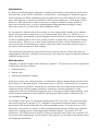
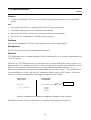
To illustrate this distinction, suppose that – over a particular period of time – we wish to execute four
tasks (Task A, Task B, Task C, Task D) as illustrated in Figure 1.
A
B
C
D
Time
Figure 1: A schematic representation of four tasks (Task A, Task B, Task C, Task D) which we wish to
schedule for execution in an embedded system with a single CPU.
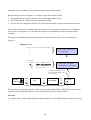
We assume that we have a single processor. As a result, what we are attempting to achieve is shown
in Figure 2.
-6-
AB
C
D
Time
Figure 2: Attempting the impossible: Task A and Task B are scheduled to run simultaneously.
In this case, we can run Task C and Task D as required. However, Task B is due to execute before
Task A is complete. Since we cannot run more than one task on our single CPU, one of the tasks has
to relinquish control of the CPU at this time.
In the simplest solution, we schedule Task A and Task B co-operatively. In these circumstances we
(implicitly) assign a high priority to any task which is currently using the CPU: any other task must
therefore wait until this task relinquishes control before it can execute. In this case, Task A will
complete and then Task B will be executed (Figure 3).
A
B
C
D
Time
Figure 3: Scheduling Task A and Task B co-operatively.
Alternatively, we may choose a pre-emptive solution. For example, we may wish to assign a higher
priority to Task B with the consequence that – when Task B is due to run – Task A will be
interrupted, Task B will run, and Task A will then resume and complete (Figure 4).
A- B
-A
C
D
Time
Figure 4: Assigning a high priority to Task B and scheduling the two tasks pre-emptively.
A closer look at co-operative vs. pre-emptive architectures
When compared to pre-emptive schedulers, co-operative schedulers have a number of desirable
features, particularly for use in safety-related systems (Allworth, 1981; Ward, 1991; Nissanke, 1997;
Bate, 2000). For example, Nissanke (1997, p.237) notes: “[Pre-emptive] schedules carry greater
runtime overheads because of the need for context switching - storage and retrieval of partially
computed results. [Co-operative] algorithms do not incur such overheads. Other advantages of
[co-operative] algorithms include their better understandability, greater predictability, ease of
testing and their inherent capability for guaranteeing exclusive access to any shared resource or
data.”. Allworth (1981, p.53-54) notes: “Significant advantages are obtained when using this [cooperative] technique. Since the processes are not interruptable, poor synchronisation does not give
rise to the problem of shared data. Shared subroutines can be implemented without producing reentrant code or implementing lock and unlock mechanisms”. Also, Bate (2000) identifies the
following four advantages of co-operative scheduling, compared to pre-emptive alternatives: [1] The
scheduler is simpler; [2] The overheads are reduced; [3] Testing is easier; [4] Certification
authorities tend to support this form of scheduling.
This matter has also been discussed in the field of distributed systems, where a range of different
network protocols have been developed to meet the needs of high-reliability systems (e.g. see
Kopetz, 2001; Hartwich et al., 2002). More generally, Fohler has observed that: “Time triggered
-7-
real-time systems have been shown to be appropriate for a variety of critical applications. They
provide verifiable timing behavior and allow distribution, complex application structures, and
general requirements.” (Fohler, 1999).
Solution
This pattern is intended to help answer the question: “Should you use a time-triggered co-operative
(TTC) scheduler as the basis for your reliable embedded system?”
In this section, we will argue that the short answer to this question is “yes”. More specifically, we
will explain how you can determine whether a TTC architecture is appropriate for your application,
and – for situations where such an architecture is inappropriate – we will describe ways in which you
can extend the simple TTC architecture to introduce limited degrees of pre-emption into the design.
Overall, our argument will be that – to maximise the reliability of your design – you should use the
simplest “appropriate architecture”, and only employ the level of pre-emption that is essential to the
needs of your application.
When is it appropriate (and not appropriate) to use a pure TTC architecture?
Pure TTC architectures are a good match for a wide range of applications. For example, we have
previously described in detail how these techniques can be in – for example - data acquisition
systems, washing-machine control and monitoring of liquid flow rates (Pont, 2002), in various
automotive applications (e.g. Ayavoo et al., 2004), a wireless (ECG) monitoring system
(Phatrapornnant and Pont, 2004), and various control applications (e.g. Edwards et al., 2004; Key et
al., 2004).
Of course, this architecture not always appropriate. The main problem is that long tasks will have an
impact on the responsiveness of the system. This concern is succinctly summarised by Allworth:
“[The] main drawback with this [co-operative] approach is that while the current process is
running, the system is not responsive to changes in the environment. Therefore, system processes
must be extremely brief if the real-time response [of the] system is not to be impaired.” (Allworth,
1981).
We can express this concern slightly more formally by noting that if the system must execute one of
more tasks of duration X and also respond within an interval T to external events (where T < X), a
pure co-operative scheduler will not generally be suitable.
In practice, it is sometimes assumed that a TTC architecture is inappropriate because some simple
design options have been overlooked. We will use two examples to try and illustrate how – with
appropriate design choices – we can meet some of the challenges of TTC development.
Example: Multi-stage tasks
Suppose we wish to transfer data to a PC at a standard 9600 baud; that is, 9600 bits per second.
Transmitting each byte of data, plus stop and start bits, involves the transmission of 10 bits of
information (assuming a single stop bit is used). As a result, each byte takes approximately 1 ms to
transmit.
Now, suppose we wish to send this information to the PC:
-8-
Current core temperature is 36.678 degrees
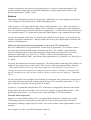
If we use a standard function (such as some form of printf()) - the task sending these 42 characters
will take more than 40 milliseconds to complete. If this time is greater than the system tick interval
(often 1 ms, rarely greater than 10 ms) then this is likely to present a problem (Figure 5).
Rs-232 Task
Time
System ‘ticks’
Figure 5: A schematic representation of the problems caused by sending a long character string on an
embedded system with a simple operating system. In this case, sending the massage takes 42 ms while
the OS tick interval is 10 ms.
Perhaps the most obvious way of addressing this issue is to increase the baud rate; however, this is
not always possible, and - even with very high baud rates - long messages or irregular bursts of data
can still cause difficulties.
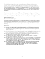
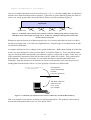
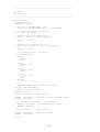
A complete solution involves a change in the system architecture. Rather than sending all of the data
at once, we store the data we want to send to the PC in a buffer (Figure 6). Every ten milliseconds
(say) we check the buffer and send the next character (if there is one ready to send). In this way, all
of the required 43 characters of data will be sent to the PC within 0.5 seconds. This is often (more
than) adequate. However, if necessary, we can reduce this time by checking the buffer more
frequently. Note that because we do not have to wait for each character to be sent, the process of
sending data from the buffer will be very fast (typically a fraction of a millisecond).
All characters
written immediately
to buffer
(very fast operation)
Current core temperature
is 36.678 degrees
Buffer
Scheduler sends one
character to PC
every 10 ms
(for example)
Figure 6: A schematic representation of the software architecture used in the RS-232 library.
This is an example of an effective solution to a widespread problem. The problem is discussed in
more detail in the pattern MULTI-STAGE TASK [Pont, 2001].
-9-
Example: Rapid data acquisition
The previous example involved sending data to the outside world. To solve the design problem, we
opted to send data at a rate of one character every millisecond. In many cases, this type of solution
can be effective.
Consider another problem (again taken from a real design). This time suppose we need to receive
data from an external source over a serial (RS-232) link. Further suppose that these data are to be
transmitted as a packet, 100 ms long, at a baud rate of 115 kbaud. One packet will be sent every
second for processing by our embedded system.
At this baud rate, data will arrive approximately every 87 µs. To avoid losing data, we would – if we
used the architecture outlined in the previous example – need to have a system tick interval of around
40 µs. This is a short tick interval, and would only produce a practical TTC architecture if a
powerful processor was used.
However, a pure TTC architecture may still be possible, as follows. First, we set up an ISR, set to
trigger on receipt of UART interrupts:
void UART_ISR(void)
{
// Get first char
// Collect data for 100 ms (with timeout)
}
These interrupts will be received roughly once per second, and the ISR will run for 100 ms. When
the ISR ends, processing continues in the main loop:
void main(void)
{
...
while(1)
{
Process_UART_Data();
Go_To_Sleep();
}
}
Here we have up to 0.9 seconds to process the UART data, before the next tick.
What should you do if a pure TTC architecture cannot meet your application needs?
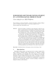
In the previous two examples, we could produce a clean TTC system with appropriate design. This
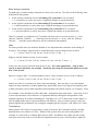
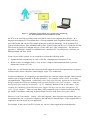
is – of course – not always possible. For example, consider a wireless electrocardiogram (ECG)
system (Figure 7).
- 10 -
Figure 7: A schematic representation of a system for ECG monitoring.
See Phatrapornnant and Pont (2004) for details.
An ECG is an electrical recording of the heart that is used for investigating heart disease. In a
hospital environment, ECGs normally have 12 leads (standard leads, augmented limb leads and
precordial leads) and can plot 250 sample-points per second (at minimum). In the portable ECG
system considered here, three standard leads (Lead I, Lead II, and Lead III) were recorded at 500 Hz.
The electrical signal were sampled using a (12-bit) ADC and – after compression – the data were
passed to a “Bluetooth” module for transmission to a notebook PC, for analysis by a clinician (see
Phatrapornnant and Pont, 2004)
In one version of this system, we are required to perform the following tasks:
•
Sample the data continuously at a rate of 500 Hz. Sampling takes less than 0.1 ms.
•
When we have 10 samples (that is, every 20 ms), compress and transmit the data, a process
which takes a total of 6.7 ms.
In this case, we will assume that the compression task cannot be neatly decomposed into a sequence
of shorter tasks, and we therefore cannot employ a pure TTC architecture.
In such circumstances, it is tempting to opt immediately for a full pre-emptive design. Indeed, many
studies seem to suggest that this is the only alternative. For example, Locke (1992) - in a widely
cited publication - suggests that “traditionally, there have been two basic approaches to the overall
design of application systems exhibiting hard real-time deadlines: the cyclic executive … and the
fixed priority [pre-emptive] architecture.” (p.37). Similarly, Bennett (1994, p.205) states: “If we
consider the scheduling of time allocation on a single CPU there are two basic alternatives: [1]
cyclic, [2] pre-emptive.” More recently Bate (1998) compared cyclic executives and fixed-priority
pre-emptive schedulers (exploring, in greater depth, Locke’s study from a few years earlier).
However, even if you cannot – cleanly - solve the long task / short response time problem, then you
can maintain the core co-operative scheduler, and add only the limited degree of pre-emption that is
required to meet the needs of your application.
For example, in the case of our ECG system, we can use a time-triggered hybrid architecture.
- 11 -
“Long” co-operative task
Pre-emptive task
Time
Sub-ticks
Tick
Figure 8: A “hybrid” software architecture. See text for details.
In this case, we allow a single pre-emptive task to operate: in our ECG system, this task will be used
for data acquisition. This is a time-triggered task, and such tasks will generally be implemented as a
function call from the timer ISR which is used to drive the core TTC scheduler. As we have
discussed in detail elsewhere (Pont, 2001: Chapter 17) this architecture is extremely easy to
implement, and can operate with very high reliability. As such it is one of a number of architectures,
based on a TTC scheduler, which are co-operatively based, but also provide a controlled degree of
pre-emption.
As we have noted, most discussions of scheduling tend to overlook these “hybrid” architectures in
favour of fully pre-emptive alternatives. When considering this issue, it cannot be ignored that the
use of (fully) pre-emptive environments can be seen to have clear commercial advantages for some
companies. For example, a co-operative scheduler may be easily constructed, entirely in a high-level
programming language, in around 300 lines of ‘C’ code. The code is highly portable, easy to
understand and to use and is, in effect, freely available. By contrast, the increased complexity of a
pre-emptive operating environment results in a much larger code framework (some ten times the
size, even in a simple implementation: Labrosse 1992). The size and complexity of this code makes
it unsuitable for ‘in house’ construction in most situations, and therefore provides the basis for a
commercial ‘RTOS’ products to be sold, generally at high prices and often with expensive run-time
royalties to be paid. The continued promotion and sale of such environments has, in turn, prompted
further academic interest in this area. For example, according to Liu and Ha, (1995): “[An]
objective of reengineering is the adoption of commercial off-the-shelf and standard operating
systems. Because they do not support cyclic scheduling, the adoption of these operating systems
makes it necessary for us to abandon this traditional approach to scheduling.”
Related patterns and alternative solutions
We highlight some related patterns and alternative solutions in this section.
Implementing a TTC Scheduler
The following patterns describe different implementations of TTC schedulers:
•
•
•
*
†
‡
TTC-SL SCHEDULER*
TTC-ISR SCHEDULER†
TTC-DISPATCH SCHEDULER‡
This is a revised version of the pattern SUPER LOOP (Pont, 2001).
This pattern is described later in this report.
We have not – to date - published a description of this pattern.
- 12 -
•
TTC SCHEDULER*
Alternatives to TTC scheduling
If you are determined to implement a fully pre-emptive design, then Jean Labrosse (1999) and
Anthony Massa (2003) discuss – in detail – the construction of such systems.
Reliability and safety implications
For reasons discussed in detail in the previous sections of this pattern, co-operative schedulers are
generally considered to be a highly appropriate platform on which to construct a reliable (and safe)
embedded system.
Overall strengths and weaknesses
☺ Tends to result in a system with highly predictable patterns of behaviour.
Inappropriate system design using this approach can result in applications which have a
comparatively slow response to external events.
Further reading
Allworth, S.T. (1981) “An Introduction to Real-Time Software Design”, Macmillan, London.
Ayavoo, D., Pont, M.J. and Parker, S. (2004) “Using simulation to support the design of distributed
embedded control systems: A case study”. In: Koelmans, A., Bystrov, A. and Pont, M.J.
(Eds.) Proceedings of the UK Embedded Forum 2004 (Birmingham, UK, October 2004).
Published by University of Newcastle.
Baker, T.P. and Shaw, A. (1989) "The cyclic executive model and Ada", Real-Time Systems, 1(1):
7-25.
Bate, I.J. (1998) "Scheduling and timing analysis for safety critical real-time systems", PhD thesis,
University of York, UK.
Bate, I.J. (2000) “Introduction to scheduling and timing analysis”, in “The Use of Ada in Real-Time
System” (6 April, 2000). IEE Conference Publication 00/034.
Bennett, S. (1994) “Real-Time Computer Control” (Second Edition) Prentice-Hall.
Cottet, F. and David, L. (1999) “A solution to the time jitter removal in deadline based scheduling of
real-time applications”, 5th IEEE Real-Time Technology and Applications Symposium WIP, Vancouver, Canada, pp. 33-38.
Edwards, T., Pont, M.J., Scotson, P. and Crumpler, S. (2004) “A test-bed for evaluating and
comparing designs for embedded control systems”. In: Koelmans, A., Bystrov, A. and Pont,
M.J. (Eds.) Proceedings of the UK Embedded Forum 2004 (Birmingham, UK, October
2004). Published by University of Newcastle.
Fohler, G. (1999) “Time Triggered vs. Event Triggered - Towards Predictably Flexible Real-Time
Systems”, Keynote Address, Brazilian Workshop on Real-Time Systems, May 1999.
Hartwich F., Muller B., Fuhrer T., Hugel R., Bosh R. GmbH, (2002), Timing in the TTCAN
Network, Proceedings 8th International CAN Conference.
Jerri, A.J. (1977) “The Shannon sampling theorem: its various extensions and applications a tutorial
review”, Proc. of the IEEE, vol. 65, n° 11, p. 1565-1596.
*
This is a generic version of the pattern CO-OPERATIVE SCHEDULER (Pont, 2001).
- 13 -
Key, S. and Pont, M.J. (2004) “Implementing PID control systems using resource-limited embedded
processors”. In: Koelmans, A., Bystrov, A. and Pont, M.J. (Eds.) Proceedings of the UK
Embedded Forum 2004 (Birmingham, UK, October 2004). Published by University of
Newcastle.
Kopetz, H. (1997) “Real-time systems: Design principles for distributed embedded applications”,
Kluwer Academic.
Labrosse, J. (1999) “MicroC/OS-II: The real-time kernel”, CMP books. ISBN: 0-87930-543-6.
Liu, J.W.S. and Ha, R. (1995) “Methods for validating real-time constraints”, Journal of Systems and
Software.
Locke, C.D. (1992) “Software architecture for hard real-time systems: Cyclic executives vs. Fixed
priority executives”, The Journal of Real-Time Systems, 4: 37-53.
Mart, P., Fuertes, J. M., Villเ, R. and Fohler, G. (2001), "On Real-Time Control Tasks
Schedulability", European Control Conference (ECC01), Porto, Portugal, pp. 2227-2232.
Massa, A.J. (2003) “Embedded Software Development with eCOS”, Prentice Hall. ISBN: 0-13035473-2.
Nissanke, N. (1997) “Realtime Systems”, Prentice-Hall.
Phatrapornnant, T. and Pont, M.J. (2004) "The application of dynamic voltage scaling in embedded
systems employing a TTCS software architecture: A case study", Proceedings of the IEE /
ACM Postgraduate Seminar on "System-On-Chip Design, Test and Technology",
Loughborough, UK, 15 September 2004. Published by IEE. ISBN: 0 86341 460 5 (ISSN:
0537-9989)
Pont, M.J. (2001) “Patterns for Time-Triggered Embedded Systems: Building Reliable Applications
with the 8051 Family of Microcontrollers”, Addison-Wesley / ACM Press. ISBN: 0-201331381.
Pont, M.J. (2002) “Embedded C”, Addison-Wesley. ISBN: 0-201-79523-X.
Pont, M.J. (2004) “A “Co-operative First” approach to software development for reliable embedded
systems”, invited presentation at the UK Embedded Systems Show, 13-14 October, 2004.
Presentation available here: www.le.ac.uk/eg/embedded
Proctor, F. M. and Shackleford, W. P. (2001), "Real-time Operating System Timing Jitter and its
Impact on Motor Control", proceedings of the 2001 SPIE Conference on Sensors and
Controls for Intelligent Manufacturing II, Vol. 4563-02.
Shaw, A.C. (2001) “Real-time systems and software” John Wiley, New York.
[ISBN 0-471-35490-2]
Torngren, M. (1998) "Fundamentals of implementing real-time control applications in distributed
computer systems", Real-Time Systems, vol.14, pp.219-250.
Ward, N. J. (1991) “The static analysis of a safety-critical avionics control system”, in Corbyn, D.E.
and Bray, N. P. (Eds.) “Air Transport Safety: Proceedings of the Safety and Reliability
Society Spring Conference, 1991” Published by SaRS, Ltd.
- 14 -
TTC-ISR SCHEDULER
{pattern}
Context
•
You have decided that a TTC PLATFORM will provide an appropriate basis for your embedded
system.
and
•
Your application will have a single periodic task (or a single transaction).
•
Your task / transaction has firm or hard timing constraints.
•
There is no risk of task overruns (or occasional overruns can be tolerated).
•
You need to use a minimum of CPU and memory resources.
Problem
How can you implement a TTC PLATFORM which meets the above requirements?
Background
See TTC PLATFORM for relevant background information.
Solution
TTC-ISR SCHEDULER is a simple but highly effective (and therefore very popular) implementation of
a TTC PLATFORM.
The basis of a TTC-ISR SCHEDULER is an interrupt service routine (ISR) linked to the overflow of a
hardware timer. For example, see Figure 9. Here we assume that one of the microcontroller’s timers
has been set to generate an interrupt once every 10 ms, and thereby call the function Update().
When not executing this interrupt service routine (ISR), the system is “asleep”. The overall result is
a system which has a 10 ms “tick interval” (sometimes called a “major cycle”) which – in this case –
involves execution of a transaction consisting of a sequence of three tasks.
BACKGROUND
PROCESSING
FOREGROUND
PROCESSING
while(1)
{
Go_To_Sleep();
}
void Update(void)
{
TaskA();
TaskB();
TaskC();
}
10ms timer
Figure 9: A schematic representation of a simple TTC scheduler (“cyclic executive”).
The end result of this activity is the sequence of function calls illustrated in Figure 10.
- 15 -
TaskA()
TaskB()
TaskC()
TaskA()
System ‘ticks’
TaskB()
TaskC()
TaskA()
...
Time
10 ms
Figure 10: The sequence of task executions resulting from the architecture shown in Figure 9.
Please note that “putting the processor to sleep” means moving it into a low-power (“idle”) mode.
Most processors have such modes, and their use can – for example – greatly increase battery life in
embedded designs. Use of idle modes is common but not essential. For example, Figure 11 shows a
simple implementation, with a single periodic task implemented directly using the Update function.
In this case idle mode is not used.
FOREGROUND
PROCESSING
BACKGROUND
PROCESSING
Update();
while(1)
{
; // Do “nothing”
}
One-second timer
Figure 11: A schematic representation of the processes involved in using interrupts. See text for details.
Please note that – in both implementations - the timing observed is largely independent of the
software used but instead depends on the underlying timer hardware (which will usually mean the
accuracy of the crystal oscillator driving the microcontroller). One consequence of this is that (for
the system shown in Figure 11, for example), the successive function calls will take place at
precisely-defined intervals (Figure 12), even if there are large variations in the duration of Update().
This is very useful behaviour, and is not obtained with architectures such as TTC-SL SCHEDULER.
Update()
Update()
Update()
...
Time
System ‘ticks’
Figure 12: One advantage of the interrupt-driven approach is that the tasks will not normally suffer
from “jitter” in their start times.
Hardware resource implications
We consider the hardware resource implications under three main headings: timers, memory and
CPU load.
Timer
This pattern requires one hardware timer. If possible, this should be a timer, with “auto-reload”
capabilities: such a timer can generate an infinite sequence of precisely-timed interrupts with
minimal input from the user program.
- 16 -
Memory and CPU Load
The scheduler will consume no significant CPU resources: short of implementing the application
using a SUPER LOOP SCHEDULER (with all the disadvantages of this rudimentary architecture), there
is generally no more efficient way of implementing your application in a high-level language.
Reliability and safety implications
In this section we consider some of the key reliability and safety implications resulting from the use
of this pattern.
Running multiple tasks
TTC-ISR Schedulers provide an excellent platform for executing a small number of tasks. If you
need to run multiple (indirectly related) tasks, particularly tasks with different periods, then you can
achieve this with a TTC-ISR SCHEDULER: however, the system will quickly become cumbersome,
and may prove difficult to debug and / or maintain.
For systems with multiple tasks, please consider using a more flexible TTC approach, such as that
described in CO-OPERATIVE SCHEDULER [Pont, 2001].
Safe use of idle mode
As we discussed in Solution, putting the processor to sleep means moving it into a low-power “idle”
mode. Most processors have several power-saving modes: when selecting a suitable mode, make
sure you choose one that (a) does not disable the timer you are using to generate the system ticks,
and (b) allows the processor to enter the normal operating mode in the event of a timer interrupt.
Note also that changing the processor mode may change the behaviour of other on-chip components
(such as watchdog timers). You must ensure that any facilities required by your application remain
operational in the idle mode which you choose.
Use of idle mode to reduce task jitter
In addition to saving power, use of idle mode can help to reduce task jitter.
This is the case because – on most processors – instructions take varying numbers of clock cycles to
execute, and your processor can only respond to an interrupt when the currently-executing
instruction has completed. For example, if your timer interrupt sometimes occurs when your
processor is at the start of a 100-cycle instruction, and sometimes occurs at the start of a 2-cycle
instruction, then the time taken to respond to the interrupt will vary considerably. By contrast, if you
use an idle mode, the time taken to return to the normal operating mode will be longer than the time
taken to respond to interrupts if the processor is fully active – but the time will not generally vary.
Overall, using idle mode can usually reduce jitter, and reduce power consumption. The only
drawback will be a very slight increase in the time taken to perform the task scheduling.
What happens if a task overruns?
With a TTC-ISR Scheduler, there will only be one active interrupt (the timer interrupt), and all tasks
are called from the timer ISR. Because ISRs cannot interrupt themselves, there is no possibility that
tasks in your system can be pre-empted. This results in highly predictable behaviour.
- 17 -
Although such behaviour is often highly desirable, it is important that you understand what happens
if a task overruns. For example, suppose that you have a task that normally takes 1 ms to execute,
and has to run every 10 ms. If –infrequently – this task takes 100 ms to execute, then the timer
“ticks” that occur in this period will be ignored.
Inevitably, there are some applications for which this is not appropriate behaviour. For example, if
you have a periodic task that keeps track of elapsed time (with a millisecond resolution), this task
must run 60,000 times every minute, without fail, or your system will lose track of the current time.
To avoid losing ticks, you may need to separate the timer ISR and the process of task execution:
patterns ISR LOOP SCHEDULER and ISR DISPATCHER SCHEDULER describe how to achieve this.
Alternatively, you may need to consider using TTH SCHEDULER, or a TASK GUARDIAN.
Strengths and weaknesses
☺ An efficient environment for running a single periodic task or periodic transaction.
Only appropriate for applications which can be implemented cleanly using a single task.
Related patterns and alternative solutions
Please also consider the following implementations of TTC Platform:
•
•
•
•
TTC-SL SCHEDULER
TTC-ISR SCHEDULER
TTC-DISPATCH SCHEDULER
TTC SCHEDULER
TTC-ISR SCHEDULER can be particularly effective if used in combination with MULTI-STATE TASK.
Further reading
-
- 18 -
TTC-ISR SCHEDULER [C, LPC2000]
{pattern implementation example}
Context
•
You wish to implement a TTC-ISR SCHEDULER [this report]
•
Your chosen implementation language is C*.
•
Your chosen implementation platform is the Philips LPC2000 family of (ARM7-based)
microcontrollers.
Problem
How can you implement a TTC-ISR SCHEDULER for the Philips LPC2000 family of
microcontrollers?
Solution
We describe how to implement a TTC-ISR SCHEDULER for the LPC2000 family of microcontrollers
in this section.
Timers and interrupts on the LPC2000 family
The ARM core at the heart of the LPC2000 family has seven interrupt sources (see Table 1).
Interrupt
Description
Reset
Caused by a chip reset.
Undefined instruction
An attempt has been made to execute an instruction with is not recognised.
Software interrupt
The software interrupt instruction can be used for calls to an operating
system (sometimes known as a “supervisor call”).
Prefetch abort
Caused by an instruction fetch memory fault.
Data abort
Caused by a data fetch memory fault.
IRQ
Used for programmer-defined interrupts which are not handled in FIQ
mode.
FIQ
This provides the fastest way of responding to programmer-defined
interrupts. This is generally used for handling a single critical interrupt: in
this book, it will almost always be used for handling timer interrupts.
Table 1: Interrupt sources from the ARM7 core.
Behaviour is as follows (see Furber, 2000):
1. Change to the operating mode corresponding to the exception
2. Save the address of the next instruction in r14 of the new mode
3. Save the old value of the CPSR in the SPSR of the new mode
4. Disable IRQs by setting bit 7 of the CPSR and, if the exception is a fast interrupt, disable further
fast interrupts by setting bit 6 of the CPSR
5. Set the PC to the relevant vector address (above table).
*
The examples in the pattern were created using the GNU C compiler, hosted in a Keil uVision 3 IDE.
- 19 -
Normally the vector address will contain a branch to the relevant routine.
Return behaviour from exceptions is as follows (again from Furber, 2000):
1. Any modified user registers must be restored from the handler’s stack.
2. The CPSR must be restored from the appropriate SPSR.
3. The PC must be changed back to the relevant instruction address in the user instruction stream.
Note that the FIQ mode has additional private registers to give better performance by avoiding the
need to save user registers. It is therefore the logical way of handling our timer interrupt in this
scheduler.
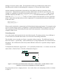
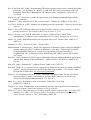
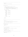
The process of handling an FIQ interrupt from the timer hardware in this way is summarised in
Figure 13.
Example code:
void Interrupt_Function(void)
{
...
}
FIQ_ISR:
STMFD
BL
LDMFD
SUBS
R13!, {R0-R7,R14}
Interrupt_Function
R13!, {R0-R7,R14}
PC, R14, #4
}
Interrupt function
(C language)
}
Interrupt wrapper
(assembly language)
(Link between timer interrupt and the
assembly-language wrapper is set up
in the “startip” file.)
Crystal
oscillator
“Fosc”
“cclk”
PLL
“pclk”
VPB divider
Timer
Figure 13: Interrupt handling (timers) in the LPC2000 family.
The operation of the phase-locked loop (PLL) and VLSI Peripheral Bus (VPB) divider may be clear
from the code example that follows: if not, Philips (2004) provides further details.
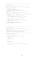
Example
A complete code example illustrating the implementation of a TTC-ISR Scheduler is given in Listing
1.
- 20 -
/*------------------------------------------------------------------*main.c (v1.00)
-----------------------------------------------------------------A simple "Hello Embedded World" test program for LPC2129 family.
(P1.16 used for LED output)
-*------------------------------------------------------------------*/
// Device header (from Keil)
#include <lpc21xx.h>
// Oscillator / resonator frequency (in Hz)
// e.g. (10000000UL) when using 10 MHz oscillator
#define FOSC (12000000UL)
// Between 1 and 32
#define PLL_MULTIPLIER (5U)
// 1, 2, 4 or 8
#define PLL_DIVIDER (2U)
// 1, 2 or 4
#define VPB_DIVIDER (1U)
// CPU clock
#define CCLK (FOSC * PLL_MULTIPLIER)
// Peripheral clock
#define PCLK (CCLK / VPB_DIVIDER)
#define PLL_FCCO_MIN (156000000UL)
#define PLL_FCCO_MAX (320000000UL)
#define CCLK_MIN (10000000UL)
#define CCLK_MAX (60000000UL)
// Function prototypes
void LED_FLASH_ISR_Init(void);
void LED_FLASH_ISR_Change_State(void);
void System_Init(void);
int PLL_Init(void);
int VPB_Init(void);
void MAM_Init(void);
void Set_Interrupt_Mapping(void);
- 21 -
/*..................................................................*/
int main()
{
// Set up PLL, VPB divider and MAM (disabled)
System_Init();
// Prepare to flash LED
LED_FLASH_ISR_Init();
while(1) // Super Loop
{
// Enter idle mode
PCON = 1;
}
// Should never reach here ...
return 1;
}
// ------ Private constants ---------------------------------------// Interrupt mapping set through the "target" settings in the IDE
#ifndef RAM
#define MAP 0x01
#else
#define MAP 0x02
#endif
/*------------------------------------------------------------------*System_Init()
Configures:
- PLL
- VPB divider
- Memory accelerator module
- Interrupt mapping
-*------------------------------------------------------------------*/
void System_Init(void)
{
// Set up the PLL
if (PLL_Init() != 0)
{
while(1); // PLL error - stop
}
// Set up the VP bus
if (VPB_Init() != 0)
{
while(1); // VPB divider error - stop
}
// Set up the memory accelerator module
MAM_Init();
// Control interrupt mapping
Set_Interrupt_Mapping();
}
- 22 -
/*------------------------------------------------------------------*PLL_Init()
Set up PLL.
-*------------------------------------------------------------------*/
int PLL_Init(void)
{
unsigned int Fcco;
unsigned int PLL_tmp;
// Cclk will be PLL_MULTIPLIER * FOSC
// Fcco will be PLL_MULTIPLIER * FOSC * 2 * PLL_DIVIDER
// To allow us to check the frequencies
Fcco = CCLK * PLL_DIVIDER * 2;
// Check that the cclk frequency is OK
if ((CCLK > CCLK_MAX) || (CCLK < CCLK_MIN))
{
return 1; // Error
}
// Check that the CCO frequency is OK
if ((Fcco > PLL_FCCO_MAX) || (Fcco < PLL_FCCO_MIN))
{
return 1; // Error
}
// Set up PLLCFG register - the divider
switch (PLL_DIVIDER)
{
case 1:
PLL_tmp = 0;
break;
case 2:
PLL_tmp = 0x20;
break;
case 4:
PLL_tmp = 0x40;
break;
case 8:
PLL_tmp = 0x40;
break;
default:
return 1;
}
// Error
// Set up the PLLCFG register - now the multiplier
PLL_tmp |= PLL_MULTIPLIER - 1;
// Apply the calculated values
PLLCFG |= PLL_tmp;
PLLCON = 0x00000001;
// Enable the PLL
PLLFEED = 0x000000AA; // Update PLL registers with feed sequence
PLLFEED = 0x00000055;
while (!(PLLSTAT & 0x00000400)) // Test Lock bit
{
PLLFEED = 0x000000AA; // Update PLL with feed sequence
PLLFEED = 0x00000055;
}
PLLCON = 0x00000003;
// Connect the PLL
PLLFEED = 0x000000AA; // Update PLL registers
PLLFEED = 0x00000055;
return 0;
}
- 23 -
/*------------------------------------------------------------------*VPB_Init()
Demonstrates setup of VPB divider
-*------------------------------------------------------------------*/
int VPB_Init(void)
{
// Input to VPB divider is output of PLL (cclk)
//
//
//
//
//
VPB
0 0
0 1
1 0
1 1
divider consists of two bits
- VPB bus clock is 25% of processor clock [DEFAULT]
- VPB bus clock is same as processor clock
- VPB bus clock is 50% of processor clock
- Reserved (no effect - previous setting retained)
switch (VPB_DIVIDER)
{
case 1:
VPBDIV &= 0xFFFFFFFC;
VPBDIV |= 0x00000001;
break;
case 2:
VPBDIV &= 0xFFFFFFFC;
VPBDIV |= 0x00000002;
break;
case 4:
VPBDIV &= 0xFFFFFFFC;
break;
default:
return 1;
}
// Error
// OK
return 0;
}
/*------------------------------------------------------------------*MAM_Init()
Set up the memory accelerator module.
NOTE: Here we DISABLE the MAM, for maximum predictability.
Adapt as needed for your application.
-*------------------------------------------------------------------*/
void MAM_Init(void)
{
// Turn off MAM
MAMCR = 0;
}
/*------------------------------------------------------------------*Set_Interrupt_Mapping()
Remaps interrupts to RAM or Flash memory, as required.
For Flash, MAP = 0x01
For RAM, MAP = 0x02
Here, value is set through Keil uVision
(depending on target built).
-*------------------------------------------------------------------*/
void Set_Interrupt_Mapping(void)
{
MEMMAP = MAP;
}
- 24 -
/*------------------------------------------------------------------*LED_FLASH_ISR_Init()
Prepare for LED_FLASH_ISR_Change_State() function - see below.
-*------------------------------------------------------------------*/
void LED_FLASH_ISR_Init(void)
{
// First, set up the timer
// We require a "tick" every 1000 ms
// (Timer is incremented PCLK times every second)
T0MR0 = PCLK - 1;
T0MCR = 0x03;
T0TCR = 0x01;
// Interrupt on match, and restart counter
// Counter enable
VICIntSelect = 0x10;
VICIntEnable = 0x10;
// Assign "Interrupt 4" to the FIQ category
// Enable this interrupt
// Now set the mode of the I/O pin
// using the appropriate pin function select register
// Here we assume that Pin 1.16 is being used.
// First, set up P1.16 as GPIO
// Clearing Bit 3 in PINSEL2 configures P1.16:25 as GPIO
PINSEL2 &= ~0x0008;
// Now set P1.16 to output mode
// through the appropriate IODIR register
IODIR1 = 0x00010000;
}
/*------------------------------------------------------------------*LED_FLASH_ISR_Update()
Changes the state of an LED (or pulses a buzzer, etc) on a
specified port pin.
Must call at twice the required flash rate: thus, for 1 Hz
flash (on for 0.5 seconds, off for 0.5 seconds),
this function must be called twice a second.
-*------------------------------------------------------------------*/
void LED_FLASH_ISR_Update(void)
{
static int LED_state = 0;
// Change the LED from OFF to ON (or vice versa)
if (LED_state == 1)
{
LED_state = 0;
IOCLR1 = 0x10000;
}
else
{
LED_state = 1;
IOSET1 = 0x10000;
}
// After interrupt, reset interrupt flag (by writing "1")
T0IR = 0x01;
}
- 25 -
/*------------------------------------------------------------------*LOOP_DELAY_Wait()
Delay duration varies with parameter.
Parameter is, *ROUGHLY*, the delay, in milliseconds,
on 12.0 MHz LPC2129 (no PLL used).
You *WILL* need to adjust the timing for your application!
-*------------------------------------------------------------------*/
void LOOP_DELAY_Wait(const unsigned int DELAY)
{
unsigned int x,y,z;
for (x = 0; x <= DELAY; x++)
{
for (y = 0; y <= 1000; y++)
{
z = z + 1;
}
}
}
/*------------------------------------------------------------------*Trap_Interrupts()
Interrupt trap - see Chapter 3.
-*------------------------------------------------------------------*/
void Trap_Interrupts(void)
{
// *** Basic behaviour ***
// DISABLE ALL INTERRUPTS
VICIntEnClr = 0xFFFFFFFF;
while(1);
}
/*------------------------------------------------------------------*---- END OF FILE -------------------------------------------------*------------------------------------------------------------------*/
Listing 1: Implementing a TTC-ISR Scheduler for the LPC2000 family (example).
Further reading
Philips (2004) “LPC2119 / 2129 / 2194 / 2292 / 2294 User Manual”, Philips Semiconductors, 3 February,
2004.
Furber, S. (2000) “ARM System-on-Chip Architecture”, Addison-Wesley.
- 26 -