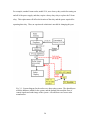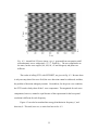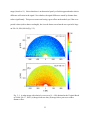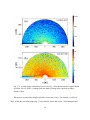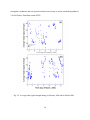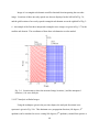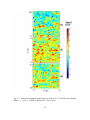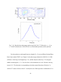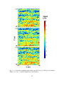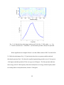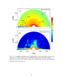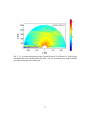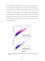
1
Project Report
X-band Radar Wave Observation System
Submitted
to
Minerals Management Service
U. S. Department of the Interior
381 Elden Street
Herndon, VA 22070
By
Jerome P.-Y. Maa, Ph.D.
and
Ho Kyung Ha
Virginia Institute of Marine Science
College of William and Mary
Gloucester Point, Virginia 23062
December 2005
Marine X-band Radars for Wave Observations
Table of Content ……………………………………………………………………. ii
Table of Figure..…………………………………………………………………….. iv
Chapter 1. Introduction.……………………………………………………………..
1
Chapter 2. Hardware Considerations ..…………………………………………….
2.1. X-band Radar ..….…………………………………..………………….
2.2. Basic Characteristics of Radar Images ……..…………………………
2.3. Personal Computer …………………………………………………….
2.4. Micro-controller ………………………………………………………..
2.5. Available High-speed ADC Interface ………………………………….
2.6. Selection of ADC Rate ………………………………….……………..
2.7. Blind Zone ……………………………………………………………..
5
5
9
12
13
15
16
18
Chapter 3. Data Acquisition ………………………………………………………… 19
3.1. System Control …………………………………………………………. 19
3.2. Batch File for PC Programs Control ……………………………………. 21
3.3. Signal Wires for Trigger and Radar Images ……………………………. 22
3.4. C program for Radar Image Data Acquisition ………………………….. 25
Chapter 4. Software for Data Analysis ……………………………………………… 31
4.1. Principle of Data Analysis ……………………………………………… 31
4.1.1. 1-D wave spectrum analysis …………………………………….. 31
4.1.2. 2-D wave spectrum analysis ……………………………………... 33
4.1.3. 3-D wave spectrum analysis ……………………………………... 36
4.2. Given Regular Wave Fields ……………………………………………. 40
4.3. A Given Random Wave Field …………………………………………. 48
Chapter 5. Data Process for Radar Images ………………………………………….. 52
5.1. Minimize Signal Distortion ……………………………………………... 52
5.2. Average Radar Signal Strength, Sa ……………………………………... 57
5.3. Interpreting Radar Image for a Small Rectangular Domain ……………. 57
5.4. FFT Analysis on Radar Images ………………………………………… 60
5.5. The Average Radar Image ……………………………………………… 71
Chapter 6. Calibration of X-band Radar Wave Measurements ……………………. 74
6.1. Star Wave Gauge ……………………………………………………… 74
6.2. Data Analysis ………………………………………………………….. 77
6.3. Measurement Results ………………………………………………….. 77
6.4. Wave Data from CHLV2 and VA001 …………………………………. 84
6.5. Signal Noise Ratio (SNR) ……………………………………………… 87
6.6. Results ………………………………………………………………….. 89
ii
Chapter 7. Remote Access ……………………………….…………………………. 92
7.1. General Requirements ………………………………………………… 92
7.2. Remote Control and Access by LAN …………………………………. 92
7.3. Remote Access by Modem ……………………………………………. 95
7.4. Software for Remote Control …………….……………………………. 96
Chapter 8. Discussion and Conclusions …………….……………………………… 98
8.1. Improvements on Hardware …………….……………………………... 98
8.2. Limitations ……………………………………………………………. 101
8.3. Other Features ………………………………………………………… 103
8.4. A Tool to Verify Numerical Model Results ………………………….. 104
8.5. Conclusions …………………………………………………………… 104
References ……………………………….………………………………………… 106
Appendix I: A BASIC program runs in the TFX-11 for controlling the PC and the radar
(In attached CD only).
Appendix II: C program codes for acquiring radar images (In attached CD only).
There are two C programs (killtime.c and radar.c) and one control input file
(radar_single.con) in this appendix.
Appendix III: Matlab® codes for analyzing the radar images for waves (In attached CD
only).
There are two Matlab main programs and six functions in this appendix. The first
main program is “imgplt.m” which is only used to read and plot the raw radar images.
This program calls two functions “read_radar_header.m” and “read_radar_image_chk.m”
to carry out the job.
The other main program is “fft3d_radar.m” which is the wave analysis program. It
calls the following functions “read_radar_header.m”, “read_radar_image.m”,
“fft3dSNR.m”, “Jacobian.m”, and “circle.m” to accomplish the job.
iii
Table of Figures
Fig. 2-1. Setup of a X-band radar at a building roof. ………………………………… 7
Fig. 2-2. The better working area, Lb, of a radar wave observation system. ………… 8
Fig. 2-3. Relationship between radar antenna height and the better working area. Lb
is for an impinge angle of 1o and Lf is for a possible extension of the better working
area by increasing the impinge angle to 0.5o. …………………………………………. 9
Fig. 2-4. For a FURUNO FR8251 radar, the radar scanning domain can be specified.
(a) Within this domain, pulses are generated from the radar control unit at a rate of
2100 pulses/s to trigger the burst of radar waves. (b) Details pulses pattern within the
scanning domain. These pulses were also used to trigger the ADC conversion. …….. 11
Fig. 2-5. Scheme diagram of the PC and radar auto-control. ………………………… 14
Fig. 3-1. System diagram for the radar wave observation system. The dotted boxes
mark the hardware installed, and the dashed lines mark the flow of control signals and
radar image of the system. All the solid boxes are from the radar manufacturer. ….… 20
Fig. 3.2. Wiring diagram for turning on and off of a FURUNO 8251 radar………….. 21
Fig. 3.3. Wires that soldered to the radar cable connector that goes to the radar
control and monitoring unit for triggering signals. The echo signal wire in a coaxial
cable is also marked……………………………………………………………………. 24
Fig. 3-4. A sketch to show the algorithm for finding the first trigger pulse, P1, when
the data acquisition software starts. This algorithm requires a radar has the capability
of setting an angular sector for observation. Between time t1 and t2, there is no trigger
signal…………………………………………………………………………………… 26
Fig. 3-5. The field experiment site, Virginia Beach, VA……………………………… 28
Fig. 3-6. An example of the radar images obtained at the Virginia Beach on 18:00,
Feb. 17, 2004. (a) All the radar burst lines (1750) are used for image plot, (b) only
437 burst lines are used for the image…………………………………………………. 29
Fig. 3-7. Sketch to show the image distortion caused by side (or side lobe) effect when
there is a strong echo at near field (< 500 m from radar). Echoes from breaking wave
foams at a distance Lb from the radar exceeds the echo strength at the true distance Lt
which is calculated by the EM wave travel speed and the time duration after trig……. 30
Fig. 4-1. Example of a selected time series and the results of calling FFT. (a) η(t)
with 12 componential waves, (b) energy spectrum by a direct dot product of F(f) and
the conjugate of F(f), and (c) energy spectrum after taking FFTSHIFT………………. 33
iv
Fig. 4-2. An artificial 2-D wave image, η(x, y), generated from an equation with 5
monochromatic waves with period = 4, 5, 7, 8 and 10 s. The wave amplitudes are the
same, but the wave angles (160, 100, 60, -65 and 0 degrees) and phases are
different……………………………………………………………………………….. 35
Fig. 4-3. Calculated wave directional distribution using the wave image given in the
previous figure. Direction ambiguity is associated with this 2-D FFT. Energy peaks
inside the small circles are the false signals…………………………………………… 36
Fig. 4-4. The first and the 30th images of a series of 64 artificial 2-D wave images,
η(x, y, t), generated with the conditions given in Section 4.1.3………………………. 38
Fig. 4-5. Part of the calculated wave energy directional distribution using the time
series of wave images given in the previous figure. Direction ambiguity is gone with
3-D FFT when the frequency is far below the Nyquist frequency. Only these
frequencies that have a noticeable energy (E ratio > 0.2) are plotted…………………. 39
Fig. 4-6. A plot of directional wave energy distribution at a high frequency band to
show that the direction ambiguity problem remains when closing to the Nyquist
frequency (0.5/t) = 0.25 hz. The energy in the 4th quadrant is the false signal……….. 40
Fig. 4-7. The first image of a 10 s monochromatic wave trains was generated with
H = 2 m, and goes 45 degrees from the x axis…………………………………………. 42
Fig. 4-8. Translation of wave energy distribution in the kx - ky plane into k - θ plane
is the first step to show the 3-D FFT results in one plot. Dots in the k - θ plane are
the locations of all available data after translating from the kx - ky plane . The uneven
data space in the k - θ plane calls for a new data grid with equal space in k and θ
coordinates. ……………………………………………………………….…….……… 43
Fig. 4-9. Directional spectrum obtained from analysis of the regular wave images:
T = 10 s, H = 2 m, direction = 45 deg. (a) k - θ spectrum, (b) f - θ spectrum. ……….. 44
Fig. 4-10. Linear wave spectrum obtained by integrating the f - θ spectrum for the
regular wave images with T = 10 s and H = 2 m…………………….………………… 46
Fig. 4-11. Directional spectrum obtained from analysis of the regular wave images
with T = 5 s, H = 2.83 m, direction = 100 deg. and a finer spatial resolution, x = y =
5 m. (a) Directional ambiguity problem remains for short period waves with a large
∆t = 1.6667 s. (b) When reducing ∆t = 1.25 s, the direction ambiguity problem
disappeared. …………………………………………………………………..………. 47
Fig. 4-12. First image of a series of random wave fields generated by using
DIWASP package with peak wave frequency fp = 0.1 Hz, Hs = 2.83 m, travel toward
the positive y-axis direction. ……………………………………………………….…. 49
.
v
Fig. 4-13. Results from 3-D FFT in kx - ky plane to show the directional spreading
at a frequency band close to the given peak energy frequency for the random sea
generated by using DIWASP.………………………….……………………………... 50
Fig. 4-14. Comparison of directional wave spectra. (a) Analyzed from the random
sea images generated by using DIWASP, (b) the given input spectrum.……………. .. 50
Fig. 4-15. Comparison of the analyzed line spectrum for the given random waves
images……………………………………………………………………………….…. 51
Fig. 5-1. A radar image with relatively severe sea (Sa = 410) obtained at the Virginia
Beach on 18:00, Feb. 17, 2004. (a) Image from raw data, (b) image after a process to
reduce distance effect………………………………………………………………….. 53
Fig. 5-2. A radar image with relatively severe sea (Sa = 404) obtained at the Virginia
Beach on 08:00, Feb. 18, 2004. (a) Image from raw data, (b) image after a process to
reduce distance effect…………………………………………………………………. . 54
Fig. 5-3. A radar image with relatively calm sea (Sa = 120) obtained at the Virginia
Beach on 10:00, Feb. 19, 2004. (a) Image from raw data, (b) image after a process to
reduce distance effect………………………………………………………………….. 55
Fig. 5-4. A radar image with relatively calm sea (Sa = 105) obtained at the Virginia
Beach on 21:00, Mar. 2, 2004. (a) Image from raw data, (b) image after a process to
reduce distance effect. ………………………………………………………………. .. 56
Fig. 5-5. Average radar signal strength during (a) February 2004 and (b) March 2004.
……...………………………………………………………………………………….. 58
Fig. 5-6. Location map to show the measured image location (*) and the interpreted
location (+) for wave analysis……………………………………………………….…. 60
Fig. 5-7. First three rectangular radar images on 18:00, Feb. 17, 2004 for wave
analysis. With x = y = 3 m, t = 1.66667s, domain size = 384 x 384 m. .……………….61
Fig. 5-8. Results from radar images analysis on 18:00, Feb. 17, 2004 with x = y = 3 m,
t = 1.66667s, domain size = 384 x 384 m. (a) Directional spectrum, (b) line spectrum.
The presented direction is for wave propagation direction. …………………………… 62
Fig. 5-9. Results from radar images analysis on 18:00, Feb. 17, 2004 with x = y = 5 m,
t = 1.66667s, domain size = 640x640 m. (a) Directional spectrum, (b) line spectrum….63
Fig. 5-10. Results from radar images analysis on 18:00, Feb. 17, 2004 with x = y =
8 m, t = 1.66667s, domain size =1024 x1204 m. (a) Directional spectrum, (b) line
spectrum………………………………………………………………………………... 64
vi
Fig. 5-11. First three rectangular radar images on 10:00, Feb. 19, 2004 for wave
analysis. With x = y = 5 m, t = 1.66667 s, domain size = 640 x 640 m……………. 65
Fig. 5-12. Results from radar images analysis on 10:00, Feb. 19, 2004 with x = y
= 5 m, t = 1.66667 s, domain size = 640 x640 m. (a) Directional spectrum, (b) line
spectrum ..………………………………………………………………………….. 66
Fig. 5-13. First three rectangular radar images on 21:00, Mar. 2, 2004 for wave
analysis. With x = y = 5 m, t = 1.66667 s, domain size = 640 x 640 m. ………….. 67
Fig. 5-14. Results from radar images analysis on 21:00, Mar. 2, 2004 with x = y
= 5 m, t = 1.66667 s, domain size = 640 x 640 m. (a) Directional spectrum, and (b)
line spectrum. .……………………………………………………………………… 68
Fig. 5-15. First three interpreted rectangular wave images measured on 00:00,
Feb. 21, 2004 for wave analysis. ..………………………………………………….. 69
Fig. 5-16. Radar measurement results on 00:00, Feb. 21, 2004, (a) directional
wave spectrum, and (b) line spectrum. …………………………………………….. 70
Fig. 5-17. Averaged radar images at the Virginia Beach. (a) For a relatively severe
sea on 18:00, Feb. 17, 2004 to show two wave breaking lines on the left hand side,
and (b) a relatively calm sea on 21:00, March 2, 2004. Two offshore buoy sets from
the Rudee Inlet are much clear for the calm sea……………………………..…….... 72
Fig. 5-18. Averaged radar images at the Virginia Beach on 21:00 March 19, 2004
to show signals that are not understood at this time. Two wave breaking lines on the
left hand side and a trench are also clearly seen…………………………………….. 73
Fig. 6-1. Location map for the X-band radar, the star wave gauge tripod, and the
NOAA Station CHLV2. Distance between the radar and the tripod is approximately
570 m. ...…………………………………………………………………………….. 75
Fig. 6-2. The star wave gauge. (a) On the moment of deployment; (b) coordinates
for wave spectral analysis. P1, P2 and P3 represent the location of pressure sensors.
The center of tripod was selected as the origin. Each sensor was located 0.66 m
above the seabed. …..……………………………………………………………… 76
Fig. 6-3. Time-averaged water surface elevation during the period of
measurements. This indicates a mean water depth of 8.2 m. ………..……………. 78
Fig. 6-4. Time series records from the wave gauge: (a) significant wave height (Hs),
the arrows indicate when a detailed spectrum analysis was given in Fig. 5.6, (b) peak
wave period; (c) Dominant wave direction; (d) direction of the peak period. ..…… 79
vii
Fig. 6-5. Wave roses for the period from 11:00, March 16 - 22:00, April 6, 2005. (a)
Direction of wave period, at the peak energy, and (b) dominant wave direction….. 80
Fig. 6-6. Wave condition on 1:00, March 18, 2005. (a) Directional spectrum, (b)
line spectrum….……………………………………………………………………. 81
Fig. 6-7. Wave condition on 16:00, March 23, 2005. (a) Directional spectrum, (b)
line spectrum….……………………………………………………………………. 82
Fig. 6-8. Wave condition on 10:00, March 28, 2005. (a) Directional spectrum, (b)
line spectrum….……………………………………………………………………. 83
Fig. 6-9. Wave condition on 16:00, April 2, 2005. (a) Directional spectrum, (b)
line spectrum….……………………………………………………………………. 84
Fig. 6-10. Relationship between the significant wave heights at Stas. CHLV2 and
VA001……………………………………………………………………………… 85
Fig. 6-11. Records of significant wave height at Stas. CHLV2. (a) February, (b)
March, (c) April, (d) November, and (e) December 2004…………………………. 86
Fig. 6-12. Example to show a collapsed “dispersion shell” in 2-D plot. Each
dashed circle represents the dispersion relationship between wave frequency and
wave number. The energy distribution given here is for 10:00, Feb. 19, 2004. .….. 88
Fig. 6-13. Examples to show a fraction of the “dispersion shell” with energy within
that frequency band for radar wave image measured on 10:00, Feb. 19, 2004. …… 90
Fig. 6-14. Example to show that there is no correlation between the significant
wave height and the SNR defined by Young et al. (1985)………………………….. 91
Fig. 6-15. The relationship between significant wave height, Hs and the second
definition of SNR. Wave height data are from Sta. CHLV2………………………. 91
Fig. 7-1. The window generated when running the program WaveOnLanGui for
WOL………………………………………………………………………………... 93.
Fig. 7-2. An example of the window of command prompt showing the MAC
address which is the same as the 12-digit physical address. An individual NIC has
its own MAC different with other NICs. …………………………………………… 94
Fig. 7-3. The device connection diagram for WOM using external or internal
modem………………………………………….…………………………………… 96
Fig. 8-1. A raw radar image to show the incorrect setting of radar measurement
range and the occasional missing of line image ……………………………………. 99
viii
Fig. 8-2. The incorrect setting on radar measurement range changes the image size
from that in the thin white dotted box to that in a much thicker black dashed box.
The occasional missing of line images (the blue lines) produces a strong signal
after FFT and results is that waves are always traveling in a direction parallel to the x
axis……………………………………………………………………….……….. 100
ix
Chapter 1. Introduction
Water wave observation is one of the important and difficult jobs that required to
be done for many purposes, e.g., shore protection, harbor management, navigation safety,
coastal resource management, rescue missions, etc. Traditional approaches for
accomplishing this kind of mission include using wave buoys, pressure wave gauges,
acoustic wave gauges, airplane or satellite video or radar observation, land-based HFband radar and X-band radar. The first three kinds of techniques are well-developed
techniques for direct observation of water surface elevations or water particle velocities
for estimating wave conditions. These techniques were first developed and followed the
available wave theory (mainly the linear wave theory). Thus they are prevailed in the
wave measurement market. These techniques, however, require the deployment of a
sensor or a series of sensor in the water, and thus, are expense for maintenance. In areas
that fishing activities are heavy, interference with fishing activities is inevitable and often
ends up with valuable instrument lost.
The last three approaches utilize the principle of remote sensing and obtain data
for interpreting wave conditions. A remote sensing approach has the advantage of getting
measurements over a large area using only one set of instrument, e.g., an air-borne video
or radar system.
If it is a land-based system, e.g., a High-Frequency (HF) radar or X-band radar,
the operation cost is relatively inexpensive, especially for the X-band radar if the required
study area is within a radius of 3 to 5 km. HF radars are mainly used for large area
currents and wave measurements (Gurgel et al., 1999). The instrumentation cost is also
big, on the order of millions for a system (http://wwwocean.tamu.edu/GOOS/GSCX/
1
GSCS_appendix_05.pdf). The principal for a HF and a x-band radar are the same, all use
Bragg effect to detect the scatter waves, but the selected wavelength are different. A HF
radar selects large EM wavelength (with the frequency range from 3 to 30 Mhz) to
produce Bragg scatter waves with the gravity waves itself, but a X-band radar uses short
EM waves to interact with ripples on top of the gravity waves. The operation range of
HF radars is large (normally on the order of 50 km, and can be extended to 200 km with
an antenna array) but with a relatively low resolution. Although the Hi-Res SeaSonde®
from Codar Ocean Sensors is claimed having the capability of measuring waves, the web
page cited in this paragraph, however, stated that other devices are needed for measuring
directional wave spectra.
Unlike HF radars, X-band radars are widely used for the vessel navigation
purpose and widely available on the market. For this reason, the cost for hardware is
reasonable and the use of x-band radars for wave observation, if the details are fully
documented, would be a promising alternative.
The first attempt of using X-band radars for wave observation was reported by
Young et al. (1985). At that time, radar images were recorded on papers, and then
digitized for wave data analysis. Since that attempt, continuous effort on the
development of X-band radar wave observation system has produced several commercial
products with specially designed hardware. For example, WaMos II (Borge et al., 1998;
1999; Borge and Soares, 2000; Krogstad et al.,1999; Wyatt et al., 1999; Wolf and Bell,
2001; Wyatt et al., 2003) was developed by following exactly the same principles given
by Young et al. (1985). The other type of X-band radar wave observation system is
2
Miros wave and current radar (http://www.miros.no/). Miros has no rotating radar
antenna and it is only good for a short-range (< 450 m) observation of waves.
The problem associated with these commercial products are (1) the price is
relatively high, about 4 to 5 times of the hardware cost, and (2) source codes for data
analysis and system control are not provided. This means the operation is somewhat like
a black box operation. Thus, it is not good for the academic research purposes. For this
reason, a study of the entire processes of using X-band radars was proposed for revealing
the details and the limitations on this kind observation system.
In Chapter 2, the considerations on hardware are presented. Details on how to
select a proper marine radar and other associated hardware are documented. Thus, it is
possible to extend and improve for future uses.
In Chapter 3, details of the radar image data acquisition system are presented.
The principle of system control and data acquisition software is explained.
In Chapter 4, the principal of wave spectrum analysis is presented. It starts with
the basic one-dimensional (1-D) Fast Fourier Transform (FFT), and then, advances into
two-dimensional (2-D) and three-dimensional (3-D) wave spectrum analysis. Clearly
known signals are used to demonstrate the process of this technique.
The numbers acquired in radar images, however, do not represent water surface
elevations. These numbers are also distorted because of the nature of measurements.
Thus, extra processes are required before using the 3-D FFT process for analyzing wave
characteristics. These processes are presented in Chapter 5.
Although the wave energy directional distribution and wave period at the peak
frequency can be obtained by following the technique given in Chapter 4 and the image
3
process procedures presented in Chapter 5, the significant wave height has to be
calculated by using the Signal Noise Ratio (SNR), and thus, require calibration. In
Chapter 6, the details on calibration by deploying a star wave gauge and using the results
from a nearby NOAA wave station, CHLV2, are presented.
Remote access of the data and remote control of the system is a convenient and
sometimes necessary tool to have a successful long-term operation. Possible options of
remote control using either Local Area Network (LAN) or a telephone modem are
explored. The necessary software and hardware were collected and tested. Details are
given in Chapter 7.
Chapter 8 is the discussion and conclusions. The problems encountered in this
project are discussed. Cautions and future works on using this kind of wave observation
system are also marked.
4
Chapter 2. Hardware Considerations
It is well known that inexpensive marine X-band radars can be used for wave
observations. Details on how to select a suitable marine radar and other associated
hardware, however, are not clearly documented, and thus, it is worth to discuss the details
and the criterion for these selections. These are the objectives of this chapter.
2.1. X-band Radar
X-band radars have a frequency range from 9.41 to 10.5 Ghz. Thus, the
wavelength of X-band radars varies from 2.8 to 3.2 cm in air. This is a rather important
information because this particular wavelength is approximately equal to the ripple
wavelength existed on the water surface when the wind speed is more than 3 m/s.
Although the ripple waves are not the target for the measurements, they are coexisted
with the much large gravity waves, which is the target of the measurements.
The principle of using marine X-band radar for wave measurements is using the
Bragg effect (Valenzuela, 1978) to get the scatter waves generated by interactions
between radio waves and ripple waves. This scatter waves are usually referred as the
“sea clutter noise” from radar’s point of view because the scatter waves are not the target
of a regular radar system. Because the closer the ripple wavelength and the EM
wavelength, the stronger the scatter wave strength, and thus, easier for a radar antenna to
pick up the scatter waves. For this reason, x-band radar is a better option.
The other type of marine radar (S-band radar) has a nominal frequency of 2.455
Ghz. Because the wavelength is large (about 12 cm), the scatter waves strength would be
weaker, and thus, the detectable range would be significantly smaller when comparing
5
with that for the X-band radar. For this reason, S-band is not suitable for the wave
measurement purposes.
The range of using X-band radars for wave measurements is limited by the radar’s
capability of measuring the scatter waves, and thus, limited by the available power of Xband radars. Since x-band radar is a commercial product with a few options on the
output power (e.g., 2, 4, 6, 10, 25, 50 kilowatts), the cost is reasonable compared with
other wave measurement approaches. In general, the larger the X-band radar output
power, the larger the measurement area and the measurable conditions. However, it is
also true that the hardware cost increases sharply for the large power radar. As a
practical application for a radius of 2 to 5 km, a 25 kw X-band radar is necessary. This
translates to a radar cost of $8,000 - 12,000 (cost in 2004), depending on the manufacture
and other options. By specifying a monochromic monitor for the radar, the total cost of a
25 kw X-band radar may be below $10k. For example, a Furuno 8251 marine X-band
radar meets all the above stated requirements, and thus, selected for this project.
The selection of a radar antenna may affect the resolution of radar image.
Because of the entire radar system is a commercial product, the antenna available for a
particular radar model is usually limited or fixed. For example, for a Furuno 8251 radar,
one may select a 6 ft or 8 ft long antenna. The antenna rotation speed is also limited to
24 or 36 rpm for a Furuno 8251 marine radar. In general, the longer the antenna, the
higher the spatial resolution of radar image in the radial direction. Also, the faster the
antenna rotating speed, the higher the temporal resolution of analyzed results in time
domain. For this reason, an 8 ft long open-array antenna that rotates at 36 rpm was
selected (Fig. 2-1).
6
Fig. 2-1. Setup of a X-band radar at a building roof.
Another advantage of a Furuno 8251 marine radar is that a sector of radar
detecting area can be specified. For example, when using a radar at a coastal station,
only the half circle image that facing the ocean is useful. With this capability, although
the radar antenna still rotates at the constant speed as usual, but only sends out radio
waves for the half circle that is facing the ocean. This capability avoids the unnecessary
exposure of radar operators or any creatures on the landside, even out of the harmful zone
that is about 5 meters from the radar. More details on how to uses this feature is given
later in this chapter.
The installation height of the radar for wave observation is another critical factor.
There is a better range for picking up the scatter wave signals. This range depends on the
radar wave incident angle (Fig. 2-2). The EM waves that come out of the antenna usually
7
Fig. 2-2. The better working area, Lb, of a radar wave observation system.
have a vertical spreading angle of 25o. At least half of the EM waves are wasted because
they are going above the horizon. Only the radio waves with an incident angle between
1o and 10o from the lower half of the radio waves are useful. For this reason, the
installation height and the radar output power are the two main factors that control the
range of wave observation. A simple relationship between the better observation range
and the radar elevation (Fig. 2-3) indicates that at least 30 m is necessary.
If the radar antenna can be oriented a little off horizontal and the maximum EM
wave direction can be pointed toward the sea level at a far away distance, then the better
working range may be extended, for example, up to that showed by the 0.5o line in Fig. 23. Although this is still a hypothesis, it may worth to check out in the future study.
8
Fig. 2-3. Relationship between radar antenna height and the better working area. Lb
is for an impinge angle of 1o and Lf is for a possible extension of the better working
area by increasing the impinge angle to 0.5o.
2.2. Basic characteristics of radar images
Assuming that the “sea clutter noise” is still larger than the background white
noise at a distance 5 km away from the radar. Thus, a maximum observation radius of 5
km was selected to show the characteristics of radar images collected. Later these
characteristics are also useful for helping determine the proper Analog to Digital
Conversion (ADC) rate.
The time for radar waves to travel along a beam should be first estimated. For a 5
km distance, it means a two-way travel distance of 10 km. Since the Electrical Magnetic
(EM) wave speed is 2.99792 x10⁸ m/s, the total time for getting the echo waves at 5 km
away would be 32 µs (= 2 x 5000 m / 3x10⁸ m/s).
9
During this 32 µs, for an antenna rotating speed of 36 rpm (i.e., 0.6 rps), the
antenna will rotate about 0.6*2π*32x10-6 s = 0.0001206 rad = 0.0069 degrees which is
rather a small angle. The swept footprint is about 0.6 m (= 0.000120685 x 5000 m) that
is much smaller than the lateral EM wave spreading (0.9o in the horizontal and 25o in the
vertical direction for a Furuno’s 8 ft long open array antenna), and thus, can be
considered as stationary.
The 0.9o degree horizontal spreading of the EM waves means a 78 m (= 0.017453
* 0.9 * 5000 m) footprint at 5 km away. This is to say that at a distance of 5 km away, a
subject with only 1 meter wide will be seen by the radar as a subject with a width of
around 70 m, although the target will still give the strongest image when it is directly on
the center of a radar beam. This is because the spread radar beam will see the same
target, but with a weaker echo signal. So instead of seeing a dot subject, the radar see an
arc subject with fading image on both ends that is much wider in the angular direction
than it would be.
For a Furuno 8251 marine x-band radar, it sends out 2100 pulses per second to
trigger the burst of radio wave beams for detecting subjects. For an antenna rotating
speed of 36 rpm, it means a total of 3500 bursts will be triggered for one radar image.
The generation of these pulses, however, can be controlled for an angular domain that is
facing the ocean (Fig. 2-4). This feature is helpful to (1) identify the time for starting
image acquisition, and (2) reduce the burst line number to 1750 for a half-circle radar
image.
In cases that the selected radar does not have this option of setting an angular
domain for wave observation, then the whole circle image will be examined. For this
10
situation, another signal pulse, the radar heading pulse, will be used to identify “when”
the radar antenna is pointing toward a specified direction. This heading pulse is also
shown in Fig. 2-4, but not used for this study.
Fig. 2-4. For a FURUNO FR8251 radar, the radar scanning domain can be specified.
(a) Within this domain, pulses are generated from the radar control unit at a rate of
2100 pulses/s to trigger the burst of radar waves. (b) Details pulses pattern within
the scanning domain. These pulses were also used to trigger the ADC conversion.
Depending on the selected maximum detecting range, the duration (or the
number) of sending EM waves in a burst is different. This is because the larger the
measurement distance, the more the EM waves are needed to produce enough echo
strength for the antenna to pickup. More EM waves mean longer burst duration.
Because there are many EM waves in a burst line, the radar measured subject length is
not the true subject length neither. For example, for an 80 ns burst duration, 800 EM
waves (= 80 x 10-9 s * 10 x 109 Hz) were sent out. Because all the waves will cause
11
reflection on a subject, an one-meter long subject along the track of radar wave beam will
be seen as a 24 m long subject (0.03 m * 800 waves) with the highest signal strength at
the center. For this reason, the burst duration should be kept as short as possible. In
other words, the operation range should be set at the shortest detect range for radar
operation, when it is used for wave measurements. This is a rather important information
that needs to be documented in this report.
The characteristics of radar images discussed in the above paragraphs assume that
the resolution for data digitization is infinitely high and the reflection of radar waves is
perfect. In reality, however, these will not be the cases, and thus, the radar images
collected are somewhat smeared.
2.3. Personal Computer
When a X-band radar was first used for wave measurements, the data analysis and
radar control were performed by using a Unix mini-computer. With the advance of
Personal Computer (PC), the control of radar, data acquired, and data analysis were
transferred to PC a few years ago. This study demonstrated that a PC with a Pentium 4
processor of 2.8 Ghz and Windows 2000® operation system is considered as a sufficient
PC for the task. An IDE hard disk with a capacity of 100 to 150 GB is required for
handle the huge data size. Memory with a size of 512 MB would be appropriate.
One critical requirement for the PC is that it should only has one PCI device
(usually it is the high-speed ADC interface card) installed in the PC. An AGP graphic
interface card should be used instead of a PCI graphic card. This is to avoid the possible
delay/interference of data transfer between the high-speed ADC card and the memory, or
12
the hard disk. Although the delay/interference of data transfer is not always happened,
radar image will be corrupted once it was triggered. This phenomenon did not happen
when our system was first installed, but it happened during the field experiment and took
about 6 months to identify this problem.
Since the data transfer speed for an electronic device (e.g., computer memory) is
much faster than that for a mechanic device (e.g., hard disk), a hard disk with a large
buffer memory is necessary. Currently, a hard disk with 8 MB buffer memory is not
uncommon, and thus, suggested for the wave observation system. If this condition can be
met, then other disk specifications would be immaterial.
It is worth to note that the temperature range during our experimental period may
be severe enough to cause the selected hardware not functioning properly. For this
reason, one should be aware that when the ambient temperature may fall below zero or
exceed 50o C, then an industrial grade PC, which has a operating temperature range from
-30o C to +80o C, is necessary.
For regular operation, a monitor is not required. But it would be nice to have one
for checking the processes. For this reason, any monitor would be sufficient.
2.4. Micro-controller
If power is not a concern of the radar wave observation system, then there is no
need to add a micro-controller for saving energy. In most application, however, power is
a major concern because of the difficulty to get AC power supply at a remote site. For
this reason, a micro-controller, Onset Model TFX-11, was added to the PC for turning on
the PC, the radar, and turning off the radar for saving energy as well as extending the
13
useful life of the radar. In general, a micro-controller with a real-time clock, three
channels of digital outputs for switching the PC and the radar is the minimum
requirement. An Onset TFX-11 was selected because of its simplicity for program and
minimum power requirements.
The TFX-11 micro-controller requires 7-12 VDC, 80 mA to operate at its full
load, and about 4 mA for standby conditions. For this reason, a small DC-to-DC
converter that change the PC’s 5V standby power to 12V was used to power the TFX-11
all the time (Fig. 2-5).
A Basic program (see Appendix I) run in the TFX-11 was used to turn on the PC
and the radar. It was also used to turn down the radar. The PC will turn itself off using a
free software “Quick Shutdown.”
Fig. 2-5. Scheme diagram of the PC and radar auto-control.
14
2.5. Available High-speed ADC Interface Devices.
At the time of this report writing (Fall 2005), there are four available high-speed
ADC devices available on the PC market: CompuScope 12100 (from Gage Applied
Technologies, Inc.), PCI-9820 (from ADLINK Technology, Inc.), UF2-3020 (Strategic
Test Corp.) and Handyscope 3 (from TiePie Engineering). These four devices all have a
12 bits maximum ADC rate meets or exceeds 100 Million Samples/second (MS/s).
The reason of having a minimum requirement on the ADC rate of 100 MS/s is not
the ADC rate itself, but to have a high-enough bandwidth for not distorting the radar
signals. The radar signals that transferred from a radar antenna to the radar control and
monitoring unit is an Intermediate Frequency (IF) signal with a frequency on the order of
10 Mhz. In order to maintain a high fidelity after feeding the IF signals into the ADC
device, a high-enough bandwidth for the ADC card is necessary. In general, because the
higher the ADC rate, the higher the bandwidth of the ADC device, and thus, 100 MS/s
for the ADC card is specified.
The first ADC device has the longest history on the market, and thus, has more
functions for applications, but the product design is relatively old, and thus, consumes
more energy (26 watts). It was selected because it was the only high-speed ADC card
available at the time when this project started.
The second ADC device has a better resolution (14 bits), a higher rate (130 MS/s),
and less power consumption (9 watts), but it is only available since early 2004. We have
a chance to use this card for a similar project. In general, the function available for this
card is limited for ADC only, and thus, cannot be used as an oscilloscope yet. For
15
experienced users, however, this card would be recommended because of its superior
ADC quality.
The third ADC device is available since middle 2004, but we have no chance to
test it yet. The above three ADC devices are all internal PCI cards, and thus, require a
desktop PC to work with.
The fourth ADC device (Handyscope 3) is an external USB-2 device and only
available since early 2005. The advantages of this device are (1) it comes with a 14 bits
signal generator, and (2) it can work with a notebook for data acquisition and data
analysis for less power consumption. The disadvantages, however, are (1) the software
support is not completed yet, and (2) the transfer speed limitation on USB-2 has not be
checked for radar application. Nevertheless, this may be a future option when the power
consumption is a major concern.
2.6. Selection of ADC Rate
Is it necessary to use the maximum ADC rate when digitizing a burst line image?
Also, is it necessary to digitize every burst line images? These two questions are
important and the answers also determine the image size.
Resolution in Angular Direction: The 1750 burst lines for a half circle mean a resolution
of 0.1 degrees (180 degrees/1750 scan lines). Since the antenna takes 0.833 seconds for a
half circle, the time between each scanning line will be 0.833 s/1750 = 0.476 ms. The
swept distance at 5 km away would be 5000 m * 0.476x10-3 s * 0.6 rps * 2 π = 8.97 m.
That is to say at 5 km away, the ADC digitized spatial resolution is about 9 m. Notice
16
that this number is much smaller than the horizontal angular spreading, 78 m, at 5 km
away from radar. When close to the radar, both the ADC resolution and spreading
resolution increase (because of the small radius distance), but the ratio remains the same
(78/9 = 8.6). This implies that there is no need to digitize every burst line images. If
selecting to digitize one line image for every 4 lines, it would be still good enough
because of the ratio is still much less than 8.6. For this reason, we carried out a test at the
early stage to compare the image quality for two options: (1) digitize every burst line
images, and (2) digitize one line in every 4 lines. The results show little difference, and
thus, the second option was used for the rest of data acquisition.
Resolution in Radial Direction: The burst duration (also called pulse width, 80 ns in this
case) also controls the image quality in the radial direction. For example, there are about
800 (80 x 10-9 s * 10 x 109 hz) waves emitted from the antenna during this 80 ns duration.
When the first wave of this wave train hit a target and reflected, the rest waves are still
coming, and the reflection will be continued until the end of the 80 ns. Thus, a radar see
the target for the entire 80 ns, and changes the subject length from 1 meter long in the
radial direction to an image length of 24 m (= 800 * 0.03 m, where 0.03 m is the wave
length of 10 Ghz EM wave). For this reason, the minimum length observed from radar
observation would be 24 m.
While scanning at 100 Ms/s for 32 µs to cover a range of 5 km, the number of
data collected represents a distance of 5000 m. Thus a resolution of 5000m/3200 point =
1.57 m can be found. This resolution is significantly higher than the radar image
resolution, 24 m, and thus, not necessary required. If scanning with a rate of 25 MS/s,
17
the radial resolution would be about 6.25 m, which is still much finer than that of the
image resolution. For this reason, a scanning rate of 25 to 30 MS/s would be sufficient.
Datafile Size: For a distance of 5 km, a total of 800 data points will be collected per burst
line in the duration of 32 µs for EM waves to travel 5 km and return back to the antenna.
This implies a data size of 1.6 KB (800 point x 2 byte/point). Notice that all the size
mentioned in this report is in binary format, not the ASCII format. If the same data is
saved in ASCII format, it will take much more space and much longer time to read and
write the same file.
For a half circle image with 437 burst line images, one radar image will take 700
KB for storage. Considering 64 radar images are suggested for data analysis, one
measurement will produce an image file with size about 45 MB. In just one day, the total
size of acquired image files will be around 1 GB. This is the nature that needs to be
considered.
2.7. Blind Zone
When a radar antenna emitted signal, it cannot be used to receive the echoes.
Depending on the model of radar, there is a block out time for receiving the echoes.
Usually it may take about 100 to 200 ns to clear the residual and switched for receiving
mode. Thus, a blind zone of 15 to 30 m (0.5 * time delay * 3x10⁸ m/s) is possible.
Fortunately, this can be easily measured with the radar. Just look at the radar screen, and
turning a nob for cursor control will let you read the blind distance directly from the radar
screen.
18
Chapter 3. Data Acquisition
With the understanding of hardware requirements, details of the radar image data
acquisition are presented in this chapter.
3.1. System Control
The information presented in this section is for the automatic radar system control
(Fig. 3-1). All the added hardware is placed inside the PC. The main control unit is a
micro-controller TFX-11 from the Onset Computer. The functions of this microcontroller are (1) turn on the radar at 56 minutes of each hour to warm up the radar, (2)
turn on the PC at 58 minutes of each hour to prepare for data acquisition, (3) turn on
radar operation at 59 minutes of each hour and (4) turn off the radar when the job is done
at 8 minutes of each hour. The schematic of this control is given in Chapter 2, and here
the control software and other details are presented.
A BASIC program (Appendix I) sets a digital I/O port high to turn on a NEC
PS2506 optoisolator for activating a Nais TF2-12v Telcom relay (Fig. 3-2). This relay
will close the circuit and provide a pulse to activate one of the first three functions
mentioned in the previous paragraph. For turning off the radar, two digital I/O ports are
required to set high. In general, the above settings are universal for all kinds of radar and
PC. The only two concerns are the capability of a relay to handle the electrical current
(and thus, the total power) required for the task. For example, the selected miniature
relay (i.e., Nais TF2-12v Telcom relay) and the miniature 80 mA DC-to-DC conversion
unit (change 5 V to 12 V) are sufficient for the selected Furuno 8251 radar. For a
different radar model, even from the same manufacturer, the switches may be different.
19
For example, another Furuno radar, model 1510, uses a heavy-duty switch for turning on
and off of the power supply, and thus, require a heavy-duty relay to replace the Telcom
relay. This replacement will affect the location of the relay and the power required for
operating that relay. Thus, an experienced technician is needed for changing this part.
Fig. 3-1. System diagram for the radar wave observation system. The dotted boxes
mark the hardware added for the system, and the dashed lines mark the flow of
control signals and radar image of the system. All solid boxes are from a radar
manufacturer.
20
Fig. 3.2. Wiring diagram for turning on and off of a FURUNO 8251 radar.
3.2. Batch File for Controlling the PC programs
After the PC was turned on, the Windows 2000 operation system will be loaded
automatically first. After this, a batch program, “radar.bat” will be launched
automatically by leaving this program in the “Startup” sub-folder, which is under the
folder of “C:\Documents and Settings\Start Menu\administrator\.” This batch program
contains the following five commends
c:\radar\debug\killtime.exe
c:\radar\debug\radar.exe
Move rd*.h?? d:\data\
Move rd*.b?? d:\data\
c:\autologon\shutdoen\qsd –s
21
The first commend executes a program “killtime” to let the PC idle for 100
seconds. This idle is for letting the rotating speed of radar antenna approaches a steady
condition. The second command executes the radar image data acquisition. The results
of this acquisition are two files: “RDmmddyy.hhr” and “RDmmddyy.bhr” where “RD” in
the filename stands for radar, “mm”, “dd” and “yy” will be replaced by the integer
number of the month, day and year when the data was acquired. The first “h” in the file
type stands for an ASCII header file, and the “hr” will be replaced by the integer number
of the hour when the file was created. The first character “b” in the file type stands for a
binary image data file. For example, “RD011204.h01” and “RD011204.b01” are the
header file and the image file created on January 12, 2004, 01:00. The contents in the
header file (i.e., the setup of A/D interface card, date and time, radar operation
conditions, etc.) are in ASCII format and can be seen by using any text editor. The image
file, however, is a binary file and can only be read by using a computer program.
Anyway, these two data files will be moved to another hard disk for storage. The last
command is an auto shutdown command. It will turn off the PC, and wait for the next
“turn on” given by the micro-controller.
Notice that the radar data analysis program is not included in the batch file at this
time. But it can be added later easily once an operational decision has been made.
3.3. Signal wires for trigger and radar images
In general, a marine x-band radar usually uses the same antenna for transmitting
and receiving signals. These two kinds of signals are quite different in terms of power
level. The transmitted signals usually have a power on the order of 6 to 75 Kilowatt
22
(KW) for the x-band marine radar. On the other hand, the received signals can be as low
as milliwatt. Thus, a signal amplifier is needed to boost the received signal. In order to
prevent the strong transmission signals to destroy the receiving amplifier, two devices
called “duplexer” and “limiter” were installed between the antenna and the radar
manufacturer’s receiving amplifier (Fig. 3-1). The duplexer changes to a high impedance
device when a strong signal comes to it, and thus, blocks out the high power signals.
Because there is a possibility that a signal coming from a near-by radar that is not strong
enough to ignite the duplexer but strong enough to destroy the amplifier, a “limiter” is
usually provided to limit the power that can go to the signal amplifier. The duplexer,
limiter, amplifier and rectifier are all provided by the radar manufacturer, and thus, these
are not the concerns of this project. The objective of this discussion is to point out where
the echo signals can be picked up. Further explanation on how to pick up the echo signal
is given next.
Physically, there are two units for a marine x-band radar: (1) the radar antenna
and gear head unit, and (2) the control and monitor unit. Radar waves are actually
generated in the 1st unit, but the control signals are generated in the 2nd unit. The echo
signals are also detected in the 1st unit, but pass to the 2nd unit for processing. For this
reason, there is a cable to connect these two units for signals to travel between them.
Two kinds of signals are needed for the radar image acquisition. The first kind of
signals is for “when to start the ADC?” The second kind of signals is the radar echo
signals that will be digitized. All these two kinds of signals are available from a radar
control and monitor unit provided by the radar manufacturer (see the two dashed lines in
Fig. 3-1 that comes out of the radar).
23
The connectors that hook up the radar cable to the control and monitoring unit are
the places to get these two kinds of signals (Fig. 3-3). Usually the echo signals are run in
a coaxial cable (because the weak signals require isolation from other signal lines and
power lines) that is bundled with others in the main cable that connects the two radar
units. It is relatively easy to find this line physically. The exact pin number on the
connector for trigger signals that send to the antenna unit can be found from the user
manual provided by the radar manufacture. For example, the yellow and black lines in
Fig. 3-3 are for retrieving the trigger signals and ground for a Furuno 8251 marine radar.
Although there are 4 wires in this picture, the other two wires are for the heading signals
that are not needed for this application.
Fig. 3.3. Wires that soldered to the radar cable connector that goes to the radar
control and monitoring unit for triggering signals. The echo signal wire in a coaxial
cable is also marked.
24
3.4. C program for Radar Image Data Acquisition
In a high-speed ADC interface device, there are usually two input channels for
digitization (Channel A or/and Channel B), one channel for external trigger source and
one channel for auxiliary input. The radar echo images are fed into one of the input
channel for digitization (e.g., Chan A) and the radar trigger signals are fed into the
channel for external trigger source. Because the capability of selecting a high input
impedance (e.g., 1 MΩ) for both of the channels, the hookup and splitting of these two
signals will not affect the original signal strength.
In the C programming, the first task is to find the first trigger pulse that
representing time t2 in Fig. 3-4. In this figure, t1 and t3 represent the end times of two
consecutive antenna revolutions, and t2 (with the first pulse, P1) represents the start of
radar image scanning. Because the time to start the C program is not necessary between
time t1 and t2, the first detected pulse has a quite good chance to fall between t2 and t3.
For this reason, the first task is to count how many trigger events have been received
from the external trigger source. Since the time interval between each pulse is 475 µs, if
there is no trigger event after a sufficiently long time, for example, 1000 µs, then it is
clear that the program has come to a time that is after t3. So the program just starts
waiting for the next 1st pulse that represents at time t4. If the program successfully
counted up to 1747 pulses (slightly less than the ideal 1750 pulses) with a time interval
less than 1000 µs between each pulse, this also means the program has come to a time
that is close to t3. With this situation, the program just waits a few thousand
microseconds more, and then starts to wait for the next 1st pulse at time t4.
25
Fig. 3-4. A sketch to show the algorithm for finding the first trigger pulse, P1, when
the data acquisition software starts. This algorithm requires a radar has the
capability of setting an angular sector for observation. Between time t1 and t2, there
is no trigger signal.
The above paragraph ensures that the program always starts to do ADC from the
first trigger event, which also represents to start ADC at the beginning of the selected
observation domain. After this time, a selected number of antenna revolutions (e.g., 10
turns) is skipped. During this period, the radar images are not digitized, only the number
of antenna revolution is counted. The purpose of this process is to give a little more time
for the antenna rotation to reach a steady condition.
26
The final step is to digitize radar image on the selected burst line images. It is
mentioned in Chapter 2 that not all the 1750 burst line images are required to be
digitized. This study indicates that to digitize one burst line and then skip the next three
burst lines would have sufficient image resolution, and that is how the C program was
coded.
The documentation of the above algorithm should be sufficient for readers to
follow the C program codes, which is given in Appendix II.
The radar system mentioned in Chapter 3 was setup at the roof of the Clarion
Resort and Conference Center (36o30.036’N, 75o34.935’W, Fig. 3-5), with an elevation
about 38 m above the sea surface. The shoreline (which will be used as the x axis in
radar image process) at this location has an angle about 13 degrees West from North, and
this information will be used later for determine wave directions. For example, waves
coming from E will be shown as waves coming from 77o (= 90 o – 13 o), counted from the
positive x-axis. This is equivalent to say that waves are going toward -103 o from the
radar analysis results.
An example of the radar image (Fig. 3-6) shows that a clear radar wave image can
be obtained. Notice that the wave image quality is better at the center, and gradually
degraded on the two sides that are close to the shoreline. This is possible because of the
radar wave direction is parallel to the wave crest lines. In other words, the strong wave
reflection from a rising slope do not return back to the radar because of the nearly parallel
of radar wave incident line and the wave crest line. The jetty on the north of the radar
site, the two breakwaters at the Rudee Inlet, and the wave breaking line can be seen
27
clearly in this image. At the bottom center, the solid red semi-circle marks the blind
zone.
Fig. 3-5. The field experiment site, Virginia Beach, VA.
Because of the relatively large radar wave spreading (25 degrees) in the vertical
direction and the selected radar elevation, a strong reflective subject at a distance that is
close to the radar will be seen as a subject that is further away. For example, the bright
(yellow) lines near the bottom center in Fig. 3-6 were caused by the strong reflection of
white foams on the breaking wave crests. This line should be a straight line because the
shoreline is straight at this site, but it was shown as a curve in the image. This radar
image distortion can be explained in Fig. 3-7 as the side lobe effect. The strength of echo
28
signal at the short distances, Lb, caused by the side EM waves exceeds the signal strength
that come back from the distances, Lt, that the travel times for the EM waves really
represented. If there is no side-lobe effect, then the breaking foams near the radar center
will not be seen. If the height of radar antenna is low enough or the subject is far enough
from the radar antenna, then the distortion will be negligible. Actually Fig. 3.6 indicates
that a distance about 500 m is needed to have a negligible image distortion.
Fig. 3-6. An example of the radar images obtained at the Virginia Beach on 18:00,
Feb. 17, 2004. (a) All the radar burst lines (1750) are used for image plot, (b) only
437 burst lines are used for the image.
29
Fig. 3-7. Sketch to show the image distortion caused by side (or side lobe) effect
when there is a strong echo at near field (< 500 m from radar). Echoes from
breaking wave foams at a distance Lb from the radar exceed the echo strength at the
true distance Lt which is calculated by the EM wave travel speed and the time
duration after trig.
30
Chapter 4. Software for Data Analysis
It would be better to start with the principle of wave spectrum analysis, and then,
advance into three-dimensional (3-D) wave spectrum analysis. After the flow of data
processing is explained, it would be better to use clearly known signals to demonstrate
the results of data analysis. At last, test of the program developed with images for a
random sea is presented.
4.1. Principle of Data Analysis.
First the basic one-dimensional (1-D) and two-dimensional (2-D) wave spectrum
analysis will be given briefly to introduce the concept of Fourier Transform for wave
spectrum analysis.
4.1.1. 1-D wave spectrum analysis
A time series record of water surface elevations, η(t), at a particular observation
site can be transferred into frequency domain by using the Fourier Transform defined as
follows.
∞
F ( f ) = ∫ η (t ).e −ift dt
(4-1)
−∞
where i = (-1)½, t is a dummy variable that represents time in this study, f represents
frequency. The above definition is for an infinite time series. For practical applications
with a finite length of discrete data, a Fast Fourier Transform (FFT) algorithm was
invented a long time for a reasonable number of data point, n, varies from 256 to 4096
(i.e., n = 2k and k = 8 to 12). This algorithm was implemented in Matlab® as a function
called FFT.M. Notice that the variable, t, in Eq. 4-1 can represent any physical
31
parameter, for example, spatial distance, x or y. Because the exponential component, ift,
should be a non-dimensional parameter, and thus, it is obvious that f is frequency if t is
time.
The output of calling FFT is an 1-D complex array (i.e., F(f) = R(f) + iG(f), where
R and G are the real and imaginary part of F) with the same length as that of the input
time series. The dot product of this complex array with its conjugate (i.e., R2 + G2) is
defined as the energy spectrum with a unit of m2/hz. The frequency resolution is given as
1/(n∆t), where ∆t is the time interval of water surface elevation samples. An example of
an artificially generated time series of 1024 points for water surface elevations with 12
wave components and ∆t = 2 s is given in Fig. 4-1a. The result of calculated energy
spectrum is given in Fig. 4-1b. Notice that the x-axis of Fig. 4-1b is from 0 to a
maximum of 1/∆t (0.5 Hz in this example). This is just for the convenience to plot the
FFT results quickly. Actually, the frequency domain should be started from minus
infinite (-∞) and ended at positive infinite (+∞) for an infinite time series. For a finite
length of time series, the frequency domain should be from –0.5*n/∆t to 0.5*n/∆t with
zero frequency in the center. A function FFTSHIFT for this purpose is also implemented
in Matlab®. For this 1-D case, it simply swaps the left and right halves of the computing
results indicated by the dashed array between Fig. 4-1b and 4-1c. FFTSHIFT is useful
for visualizing the Fourier Transform with the DC component (frequency = 0) in the
middle of the spectrum. The traditional way to present the spectrum is just taking the
positive half of the plot (either the left half in Fig. 4-1b or the right half of Fig. 4-1c) and
double the energy values because of the omission of energy in the negative half
frequency domain.
32
Fig. 4-1. Example of a selected time series and the results of calling FFT. (a) η(t)
with 12 componential waves, (b) energy spectrum by a direct dot product of F(f) and
the conjugate of F(f), and (c) energy spectrum after taking FFTSHIFT.
4.1.2. 2-D wave spectrum analysis
A time series record of water surface elevations at specified observation sites
along an 1-D spatial domain (here denote x), η(t, x), can be transferred into frequency
and wave number domains by using the 2-D Fourier Transform defined as follows.
F( f , k) = ∫
∞
−∞
∫
∞
−∞
η (t , x)e −ift e −ikx dtdx
(4-2)
where x represents a series of spatial locations (in unit of m) at where water surface
elevations were measured. Because kx must be a non-dimensional parameter, k must
33
have the dimension of m-1. For the convenience of using trigonometric function, a
coefficient of 2π is included in the definition of k, i.e., k = 2π/L, where L is the
wavelength. Notice that there are two dummy variables in Eq. 4-2, and these two can be
changed as t and y or x and y. In cases that x and y are selected as the two dummy
variables, then the resulting function is F(kx, ky), where the subscripts x and y are added
to represent wave number components in the x and y directions, respectively.
Similar to that for the 1-D FFT, a function for 2-D FFT for a finite length and
discrete domain (FFT2.M) is also available in Matlab®. An example of using this
function with an artificial signal is given next.
A snap shot of a wave field, η(x, y), was generated according to the following
equation:
η(x,y) = aj*cos[kj*cos(θj)*x + kj*sin(θj)*y - φj]
(4-3)
with five monochromatic wave trains, i.e., j = 5 (Fig. 4-2). All the wave amplitudes (i.e.,
ai’s) were 1 m, and the five wave periods were T = 4, 5, 7, 8 and 10 s, respectively. The
five wave directions were θ = 160, 100, 60, -65, and 0 degrees, respectively, and the five
wave phases were φ = 30, 70, 50, 20, and 0 degrees. Deep water condition was assumed,
and thus, the wave number, k, was calculated as (2π)2/(gT2). The size of the computed
wave field had 128 x 64 points with a spatial resolution of 10 m in both the x and y
directions (in other words, 1280 and 640 m in the x and y directions), respectively.
For waves in an intermediate water depth and if the water depth, h, is known, then
the wave number can also be obtained using the linear dispersion equation, σ2 = gk
tanh(kh), where σ = 2π/T.
34
Fig. 4-2. An artificial 2-D wave image, η(x, y), generated from an equation with 5
monochromatic waves with period = 4, 5, 7, 8 and 10 s. The wave amplitudes are
the same, but the wave angles (160, 100, 60, -65 and 0 degrees) and phases are
different.
The results of calling FFT2, with FFTSHIFT, are given in Fig. 4-3. Because there
is only one snap shot of the wave field, the wave direction cannot be addressed, and thus,
the problem of direction ambiguity remains. Nevertheless, for the given wave condition,
the FFT2 results clearly show all the 5 wave components. The magnitude for each wave
components, however, cannot be equal because of the requirement for the best spatial
resolution is different for each frequency.
Figure 4-3 can also be translated into energy distribution in frequency, f, and
direction, θ. This task, however, is carried out later in Sec. 4.2.
35
Fig. 4-3. Calculated wave directional distribution using the wave image given in the
previous figure. Direction ambiguity is associated with this 2-D FFT. Energy peaks
inside the small circles are the false signals.
4.1.3. 3-D wave spectrum analysis
Similar to 2-D wave spectrum analysis, a time series record of water surface
elevations at specified observation sites on a horizontal 2-D domain (here denotes as x,
y), η(t, x, y), can be transferred into frequency and two wave-number (kx and ky) domains
by using the 3-D Fourier Transform defined as follows.
F( f , kx , k y ) = ∫
∞
−∞
∞
∞
−∞
−∞
∫ ∫
η (t , x, y ).e −ift e −ikx e −iky dt.dx.dy
36
(4-4)
A function for n-dimensional FFT with a finite length of data record (FFTN.M) is
also available in Matlab®. An example of using this function with an artificial signal is
given next.
Now the wave data are n snap shots of the wave field, η(x, y, t), which was
generated according to Eq. 4-5. This equation has only one extra term (i.e., σj t) added to
produce n snap shots (Fig. 4-4 with a total of 64 snap shots with ∆t = 2 s). All other
parameters are the same as those given in the previous section except that ∆x = ∆y =
7.7985 m and the five wave directions are 160, 20, 60, -65, and 20 degrees, respectively.
η(x,y,t) = aj*cos[kj*cos(θj)*x + kj*sin(θj)*y - σj t + φj]
(4-5)
The result of calling FFTN, F(f, kx, ky) is also a 3-D complex matrix with exactly
the same dimension as that for the input η(x,y,t): 64 frequency band, 128 kx band, and 64
ky band. There are two ways to present the results in graphic form: (1) to plot the energy
distribution for each frequency band, or (2) to summary the results and plot the direction
energy distribution in one figure. In this section, the results are presented in the first form
only.
There should be at least 32 plots to present all the information. However, only
those frequency bands that have a relatively large energy are presented in Figs. 4-5 and 46. Because a series of snap shots are available, the wave directional ambiguity problem
was correctly addressed when the frequency is reasonably lower than the Nyquist
frequency (Oppenheim, 1999), i.e., 1/(2∆t) (Fig. 4-5). When close to the Nyquist
37
frequency, however, wave ambiguity problem still remains (Fig. 4-6). This is because
the time
Fig. 4-4. The first and the 30th images of a series of 64 artificial 2-D wave images,
η(x, y, t), generated with the conditions given in Section 4.1.3.
38
Fig. 4-5. Part of the calculated wave energy directional distribution using the time
series of wave images given in the previous figure. Direction ambiguity is gone with
3-D FFT when the frequency is far below the Nyquist frequency. Only these
frequencies that have a noticeable energy (E ratio > 0.2) are plotted.
39
interval between two consecutive snap shots is too big to distinguish the wave
propagation direction for that frequency band.
Fig. 4-6. A plot of directional wave energy distribution at a high frequency band to
show that the direction ambiguity problem remains when closing to the Nyquist
frequency (0.5/t) = 0.25 hz. The energy in the 4th quadrant is the false signal.
Notice that the above two figures show the energy distribution for each frequency
band. Actually, there are redundant information included in these two figures because kx
and ky also include wave frequency and wave direction information, if the linear
dispersion equation, σ2 = gk tanh(kh), is used. For this reason, the 2nd way to present the
3-D FFT results can be summarized in one single plot and that is explained in next
section.
40
4.2. Given Regular Wave Fields
Since the 3-D FFT result is a 3-D matrix that includes information for n frequency
bands, m kx bands and L ky bands, one way to present the summarized results is to add
these n frequency bands together to form a single 2-D matrix in kx - ky plane. This can be
done relatively easy by retrieving the energy density in kx - ky plane for each frequency
band and then add them together, with a multiplier of 1/(n/dt) for the true spectrum
energy.
Example of a monochromatic plane wave field (i.e., j = 1 in Eq. 4-5) was
displayed (Fig. 4-7, only show the first snap shot for this case) to demonstrate the
process. The spatial domain had 128 points in both the x and y directions, respectively,
with ∆x = ∆y = 7 m. In time domain, 32 snap shots were generated with ∆t = 1.66667 s.
The deep-water condition was used again for this example. After calling FFTN, the
results of adding up all the 32 frequency bands, φ(kx, ky), are given in Fig. 4-8a. The
spike (because of the monochromatic waves) in the first quadrant of this sub-plot shows
that the wave direction is 45 degrees. The dashed circle indicates that the wave number k
= 0.5 m-1. This sub-plot has a Cartesian coordinate system with data point on a grid with
equal intervals in the kx - ky plane, i.e., ∆kx = ∆ky = 2π/ (128 * 7 m).
Knowing that kx = k cos(θ) and ky = k sin(θ), all the values on each grid point of
this Cartesian grid can be translated to have a polar coordinate (k-θ) grid. A Matlab®
function CART2POL.M can be used to do this job. Notice that the energy value at each
grid point also changed because of the coordinate change and the following equation was
used (Young et al., 1985).
ϕ(k, θ) = k φ( kx, ky)
(4-6)
41
where ϕ(k, θ) is the wave energy distribution in k-θ plane.
Locations of these new grid points in the rectangular k-θ plane (Fig. 4-8b) show
that the distances among points are not the same, and thus, a new grid with equal space in
∆k and ∆θ, respectively, is needed. This requirement calls for interpreting the energy
values at each new grid point for the rectangular k-θ plane. A basic Matlab® function
GRIDDATA was used to do this task. After using GRIDDATA, however, one would
find that wave energy at a few grid locations (mainly with a low k coordinate and when
the θ coordinate is close to 0 or 360 degrees) are specified as “nan” which stands for “not
a numerical value.” This phenomenon was caused by not having an enough spatial
resolution for interpreting wave energy at low k values (see Fig. 4-8b), without data on
the negative θ coordinates, and without data with a θ coordinate that is large than 360
degrees, respectively. A simple treatment of this problem would be replacing the “nan”
with zero. This treatment is efficient and quite good for coastal wave observations
Fig. 4-7. The first image of a 10 s monochromatic wave trains was generated with
H = 2 m, and goes 45 degrees from the x axis.
42
Fig. 4-8. Translation of wave energy distribution in the kx - ky plane into k - θ plane
is the first step to show the 3-D FFT results in one plot. Dots in the k - θ plane are
the locations of all available data after translating from the kx - ky plane. The uneven
data space in the k - θ plane calls for a new data grid with equal space in k and θ
coordinates.
because there should be few waves that travel in parallel with the shoreline (an angle of
0, 180 or/and 360 degrees).
43
Now the wave energy distribution is presented in k-θ plane (Fig. 4-9a), and one
more step may be useful to display the wave energy directional distribution by translating
it into the most popular f-θ plane (Fig. 4-9b).
Fig. 4-9. Directional spectrum obtained from analysis of the regular wave images:
T = 10 s, H = 2 m, direction = 45 deg. (a) k - θ spectrum, (b) f - θ spectrum.
This translation follows the formula given by Young et al. (1985) as
ψ ( f ,θ ) =
dk
.ϕ (k ,θ )
df
(4-7)
where dk/df is the Jacobian matrix between ψ and ϕ. According to the wave dispersion
relationship in linear wave theory, it can be calculated as
44
4π gk tanh(kh)
dk
=
df
g tanh(kh) + gkh sec h 2 (kh)
(4-8)
Since line spectrum is quite frequently used in many applications, it is also
desirable to present the line spectrum as well. This can be done simply by adding up the
energy in all direction domains for each frequency band (Fig. 4-10).
No matter what the coordinate system a wave energy distribution is presented, the
total energy should remain the same. This can be checked by using the total volume, vo,
under a directional spectrum, or the total area, mo, under a line spectrum. This is because
the significant wave height, Hs, can be found as
H s = 4.02 mo = 4.02 v o
(4-9)
Notice, however, the Hs calculated in Eq. 4-9 is based on the random sea with a
Rayleigh distribution on wave height for unit sea surface area (Dean and Dalrymple,
1992). In other words, the effect of computing domain should be excluded. For
monochromatic waves, the input wave height specified is actually the root-mean-square
wave height (Hrms) that is Hs/1.414 For example, the given input monochromatic wave
height is 2 m that is corresponding to specify a Hs of 2.83 m. The calculated Hs during
various stages of the Matlab® program FFT3D_RADAR.M (see appendix III) are around
2.84 m. This example indicates a small error of 0.01 m for the selected settings on ∆x,
∆y, ∆t, and simulation domain. This represents an error around 0.4%.
For other tested wave periods with the same wave image domain (896 m = 128 *
7 m), image resolution (7 m x 7 m), temporal domain (53 s = 32 * 1.66667 s), and
temporal resolution (1.66667 s), the results are given in Table 4-1. In general, the result
45
is good except for the short period waves, i.e., the 5 s wave trains. The average error is
about 8% in terms of the calculated Hs, if the case for 5 s waves is excluded.
Fig. 4-10. Linear wave spectrum obtained by integrating the f - θ spectrum for the
regular wave images with T = 10 s and H = 2 m.
Table 4-1. Test results for monochromatic wave trains with a given Hs = 2.83 m.
Period (s)
5
6
7
8
9
10
12
14
Angle (deg)
100
45
130
60
45
90
130
135
Hs (m)
1.12
3.02
2.42
2.94
2.35
2.84
2.71
3.02
Error (%)
-60
6.7
3.9
-17
0.4
-14.5
46
-4.2
6.7
For 5 s waves at the deepwater condition, the wavelength is 39 m. Thus, the 9.9
m, i.e., (72 + 72)1/2, spatial resolution and 1.66667 s temporal resolution may not be good
enough. By reducing the spatial resolution, i.e., changing ∆x and ∆y to 5 m, but
maintaining ∆t = 1.66667 s, the calculated Hs improved to 1.94 m, but directional
ambiguity problem remained because of the large ∆t (Fig. 4-11a). When increasing the
temporal resolution with a smaller ∆t = 1.25 s, the directional ambiguity problem
disappeared (Fig. 4-11b). This is a clear indication that a fast rotating antenna should be
used if the expected wave period is small at a radar observation site. Also the higher the
temporal resolution, the better the results for short period waves.
Fig. 4-11. Directional spectrum obtained from analysis of the regular wave images
with T = 5 s, H = 2.83 m, direction = 100 deg. and a finer spatial resolution, x = y =
5 m. (a) Directional ambiguity problem remains for short period waves with a large
47
∆t = 1.6667 s. (b) When reducing ∆t = 1.25 s, the direction ambiguity problem
disappeared.
4.3. A Given Random Wave Field
It would be nice to check the program developed in the previous section with
images of clearly known random sea. This is not a simple task, however, and a monthlong attempt to generate this kind of images was not successful, and thus, gave up at the
early stage. Fortunately, a software package DIrectional WAves SPectrum (DIWASP)
developed at the Center for Water Research, University of Western Australia (Johnson,
2005) was available later and used successfully to generate this kind of signals. An
example of the DIWASP generated images for random sea is available on the VIMS web
site http://www.vims.edu/physical/projects/diwasp/ for showing the nature of random sea.
The 64 consecutive random sea images used for checking the 3-D FFT program
given in the previous section specified a significant wave height of 2.83 m, frequency at
the peak energy = 0.1 hz, moved toward the positive y direction (Fig. 4-12). In other
words, the major wave direction was 90 degrees from the x –axis. Other parameters were
specified as: directional spreading = 10 degrees, noise level = 25 (with a range from 0 to
100), water depth at the image site = 26 m, time interval between two consecutive images
= 1.66667 s. Each image has 128 x 128 points in the x and y direction, respectively, with
a grid resolution of 8 m in both the x and y directions.
At a frequency that is close to the wave peak energy frequency, the program
calculated directional spreading is probably more than 10 degrees (Fig. 4-13). This may
be because of the selected noise level of 25. Nevertheless, the direction is correctly
calculated as 90 degrees in the kx - ky plane. After transferred it to the f - θ plane, it can
48
be seen more clearly that the peak energy frequency is around 0.1 Hz, with a main
direction of 90 degrees (Fig. 4-14a). This time, the energy was spread over a much large
domain, caused by the nature of random sea. The given directional wave spectrum that
was used to generate the wave images was also displayed (Fig. 4-14b). A much smooth
contour plot for the given directional spectrum is evident. The line spectrum (Fig. 4-15)
also shows the results correctly and the significant wave height calculated from the
program (Hs = 2.81 m) has a negligible error of 0.7%.
Fig. 4-12. First image of a series of random wave fields generated by using
DIWASP package with peak wave frequency fp = 0.1 Hz, Hs = 2.83 m, travel toward
the positive y-axis direction.
49
Fig. 4-13. Results from 3-D FFT in kx - ky plane to show the directional spreading
at a frequency band close to the given peak energy frequency for the random sea
generated by using DIWASP.
Fig. 4-14. Comparison of directional wave spectra. (a) Analyzed from the random
sea images generated by using DIWASP, (b) the given input spectrum.
50
Fig. 4-15. Comparison of the analyzed line spectrum for the given random waves
images.
51
Chapter 5. Data Process for Radar Images
The data analysis tool presented in the previous chapter uses data generated on a
horizontal plane without any distortion. Radar images, however, are obtained from side view
with distortion. For this reason, there are a few steps that need to be done before wave analysis
can proceed. These steps are (1) reducing the signal distortion caused by different distance, (2)
judging the sea severity, (3) selecting a small rectangular sub-domain, (4) interpreting signals for
the sub-domain, and (4) analyzing the wave directional spectrum. Following the material
presented in this chapter, one should have no difficulty to understand the computer codes (in
Matlab®) for data analysis that is given in Appendix III.
5.1. Minimize Signal Distortion
Since the detected radar signal strength, S, is inverse proportional to the distance from a
subject to the radar antenna, r, according to S = f(r–3), the recorded signals for the entire radar
observation domain will be different even the sea severity is the same for the entire domain. For
example, the signal strength varies significantly from 0 to 1000 for the raw image (Fig. 5-1a).
The numbers mentioned here are integers recorded from the high speed ADC. There is no need
to transfer these integer numbers to floating numbers for voltage because these numbers does not
represent true wave heights anyway. Nevertheless, the range of these numbers represents a
significant range.
Since the attenuation of radar signal strength is proportion to r–3, an intuitive approach to
reduce the signal difference would be taking an one-third power on the signal. This will reduce
the signal difference caused by distance significantly. For example, Fig. 5-1b has a much small
52
range (from 0 to 11). Notice that there is no theoretical proof yet for this approach and a relative
difference still exists in the signal. Nevertheless, the signal difference caused by distance does
reduce significantly. This process seems not having a great effect on the naked eyes if the wave
period is short (with a short wavelength), but it can be better seen when the wave period is large
on Feb. 18, 2004, 08:00 (Fig. 5-2).
Fig. 5-1. A radar image with relatively severe sea (Sa = 410) obtained at the Virginia Beach
on 18:00, Feb. 17, 2004. (a) Image from raw data, (b) image after a process to reduce
distance effect.
53
Fig. 5-2. A radar image with relatively severe sea (Sa = 404) obtained at the Virginia Beach
on 08:00, Feb. 18, 2004. (a) Image from raw data, (b) image after a process to reduce
distance effect.
This process is particularly helpful when the sea severity is low. For example, on Feb. 19,
2004, 10:00, the raw radar image (Fig. 5-3a) just barely shows the swells. After taking the one54
third power on the raw signals, the swells are clearly shown (Fig. 5-3b). Notice, however, if the
sea is calm, then this approach cannot help too much. For example, the radar raw image on a
calm sea on March 2, 2004, 21:00 (Fig. 5-4a) hardly shows any wave clearly, and the processed
image (Fig. 5-4b) also cannot show a clear wave pattern.
Fig. 5-3. A radar image with relatively calm sea (Sa = 120) obtained at the Virginia Beach
on 10:00, Feb. 19, 2004. (a) Image from raw data, (b) image after a process to reduce
distance effect.
55
Fig. 5-4. A radar image with relatively calm sea (Sa = 105) obtained at the Virginia Beach
on 21:00, Mar. 2, 2004. (a) Image from raw data, (b) image after a process to reduce
distance effect.
The above information indicates that there is a threshold for using the x-band radar for wave
observation. It is already discussed in Chapter 2 that a minimum wind of 3 m/s is required.
Here another index, average radar signal strength (Sa) is also useful, and more are given in the
next section.
56
5.2. Average Radar Signal Strength, Sa
This parameter can be obtained relatively simple and fast. After taking the radar images,
a simple summation of all the signals on all the radar track lines can be obtained. This process
don’t have to use all the images, just one or two images would be enough because there is not
much change of this information at a time. As a matter of fact, it was found that all the first three
images produce a negligible difference in Sa.
The values of Sa for the four cases mentioned in the previous section are also given in the
figure captions. It can be seen that a minimum Sa value of 120 to 150 is necessary to see a wave
field. A summary of Sa value for the survey period in February and March of 2004 is presented
in Fig. 5-5. This figure indicates that a minimum sea severity about 120 is necessary to do the
rest analysis. In future operation, if Sa does not meet this minimum (or a later revised value),
then a calm sea may be concluded immediately, and the system can shut down immediately to
save battery energy.
5.3. Interpreting Radar Image for a Smaller Rectangular Domain
The next process is related to the FFTN requirement. Data used by calling the FFTN
must be in a rectangular domain with evenly spaced ∆x and ∆y. The selection of this rectangular
domain size and the size of ∆x and ∆y also need to be clarified, and that is the objective of this
section.
Because of the nature of radar scanning, radar data are presented in polar coordinates,
and that is why all the radar images presented so far are all having a semi-circle shape.
Converting the raw data with polar coordinates and uneven spatial resolution to a data set with
57
rectangular coordinates and even spatial resolution is necessary to use the standard algorithm for
3-D Fast Fourier Transform routine FFTN.
Fig. 5-5. Average radar signal strength during (a) February 2004 and (b) March 2004.
58
The size of the rectangular sub-domain depends on the resolution of radar image, the raw
radar image size, and the suitability of a “stationary process” within the selected sub-domain.
The last condition is a basic assumption of using FFTN, and it means the wave characteristics
(e.g., wave period, wave height, etc.) should be the same (or near the same) for the entire subdomain. In general, this assumption is not a problem for ocean waves because of the deep
waters, and thus, water depth plays no role in wave transformation, and within a radius of 2.5 to
5 km, this assumption held quite well. For coastal waves, wave characteristics change when
approaching the coast. This posts a major limitation on the size of sub-domain. Considering the
image distortion caused by side lobe effect for the near field, the image within a distance of 500
m from the radar center shall not be used, unless corrections can be made. For the purpose of
insurance for not using distorted image, selection of a sub-domain that is 600 m away from the
radar center would be better. Because of using a rectangular sub-domain, another limitation on
the maximum distance would simply means the maximum distance is about 200 m less than the
maximum radar sensing radius.
If using 128 x 128 points for a rectangular sub-domain at 600 m away from the radar
center, and considering a rectangular image resolution of 3, 5 and 8 m, the size of the subdomain would be 384 x 384 m, 640 x 640 m, and 1024 x 1024 m, respectively. Two factors (i.e.,
minimum wave period and maximum wave period) should be considered when selecting the size.
For a possible range of wave period from 5 to 14 seconds, the range of deepwater wavelength
would be from 37.5 and 306 m. In coastal areas, say with a water depth of 8 m, the wavelength
would be from 35 m to 102 m. For this reason, a grid resolution of 3, 5 or 8 m are all fine
because at least there are 4 points to represent a wave. The possible sizes of the three subdomains are all having at least 3.7 waves in the sub-domain, and thus, also reasonable.
59
Image of a rectangular sub-domain would be obtained from interpreting the raw radar
image. Locations of these unevenly spaced raw data are displayed on the left half of Fig. 5-6,
and the grid locations of an evenly spaced rectangular sub-domain are on the right half of Fig. 56. An example of the first three interpreted rectangular wave images are given in Fig. 5-7 for the
smallest sub-domain. The coordinates of these three sub-domains are also marked.
Fig. 5-6. Location map to show the measured image location (*) and the interpreted
location (+) for wave analysis.
5.4. FFT Analysis on Radar Images
Using the techniques given in the previous chapter, the analyzed directional wave
spectrum is given in Fig. 5-8a. This dominant wave propagation direction (-80 degrees, 4th
quadrant) can be translated as waves coming 100 degrees (2nd quadrant), counted from positive x
60
Fig. 5-7. First three rectangular radar images on 18:00, Feb. 17, 2004 for wave analysis.
With x = y = 3 m, t = 1.66667s, domain size = 384 x 384 m.
61
Fig. 5-8. Results from radar images analysis on 18:00, Feb. 17, 2004 with x = y = 3 m,
t = 1.66667s, domain size = 384 x 384 m. (a) Directional spectrum, (b) line spectrum.
The presented direction is for wave propagation direction.
direction. With the selection of x-axis orientation (Fig. 3-5), this direction can be translated as
waves are coming from ENE (23o = 10o + 13o). The line spectrum (Fig. 5-8b) indicates a peak
wave period of 5.3 s. When using a grid size of 5 x 5 m, the directional spectrum has a more
concentrated energy contours (Fig. 5-9a), and the line spectrum indicated a slightly different
peak wave period, 5.5 s (Fig. 5-9b). When using the largest grid (1024 x 1024 m), the
62
Fig. 5-9. Results from radar images analysis on 18:00, Feb. 17, 2004 with x = y = 5 m,
t = 1.66667s, domain size = 640x640 m. (a) Directional spectrum, (b) line spectrum.
directional spectrum and the line spectrum (Fig. 5-10) are all almost the same as those obtained
from the middle grid size (640 x 640 m). Considering the radar image resolution at 600 m away
from the radar center, a raw image resolution is less than 5 m, and thus, the middle grid size is
selected for later analysis.
63
Fig. 5-10. Results from radar images analysis on 18:00, Feb. 17, 2004 with x = y = 8 m,
t = 1.66667s, domain size =1024 x1204 m. (a) Directional spectrum, (b) line spectrum.
For the moderate sea (the significant wave height, Hs ≈ 2 m at an offshore National Buoy
Data Center station CHLV2, see Chapter 6), the radar images obtained on 10:00 Feb. 19, 2004
still show a clear large wavelength (Fig. 5-11), and the analysis results (Fig. 5-12) using the
middle resolution grid (i.e., 5 x 5 m) also show a clear dominant wave at 0.1 Hz that is moving
toward –95o. This direction is corresponding to the shore normal direction (off only by 5o),
which is 8o counter clockwise from E. Actually this wave field represents a combination of 10 s
64
Fig. 5-11. First three rectangular radar images on 10:00, Feb. 19, 2004 for wave analysis.
With x =y =5 m, t =1.66667s, domain size =640 x 640 m.
65
Fig. 5-12. Results from radar images analysis on 10:00, Feb. 19, 2004 with x = y =5 m,
t = 1.66667s, domain size = 640 x640 m. (a) Directional spectrum, (b) line spectrum.
swells and some wind waves (frequency 0.19 Hz) that all coming from E, if an 8o off from E is
neglected.
For the calm sea radar images obtained on 21:00 March 2, 2004 (Hs ≈ 0.5 m at Station
CHLV2, see Chapter 6), the first three interpreted rectangular images (Fig. 5-13) cannot show a
clear wave field, and the analysis results (Fig. 5-14) using the middle resolution grid (i.e., 5 x 5
m) also cannot show a clear dominant wave. The energy is practically spreading in all
frequencies and all directions. Although the line spectrum still shows a peak wave period of 4.8
s, this information may be meaning because of the wide spreading of energy in all directions.
66
Fig. 5-13. First three rectangular radar images on 21:00, Mar. 2, 2004 for wave analysis.
With x =y = 5 m, t = 1.66667s, domain size = 640 x 640 m.
67
Fig. 5-14. Results from radar images analysis on 21:00, Mar. 2, 2004 with x = y = 5 m,
t = 1.66667s, domain size = 640x640 m. (a) Directional spectrum, and (b) line spectrum.
With a significant wave height of about 1 m at the offshore station CHLV2 on 00:00 Feb.
21, 2004, the radar images (Fig. 5-15) just barely show the wave pattern, and the analyzed
directional spectrum (Fig. 5-16) shows the equally important long period waves (0.1 hz) goes to
–100 degrees and short period (0.2 Hz) waves goes to 40 degrees. The line spectrum indicates
more energy at the 0.2 Hz frequency band, but actually the wave energy at that frequency band
are coming from two major directions, 40 and –130 degrees.
68
Fig. 5-15. First three interpreted rectangular wave images measured on 00:00, Feb. 21,
2004 for wave analysis.
69
Fig. 5-16. Radar measurement results on 00:00, Feb. 21, 2004, (a) Directional wave
spectrum, and (b) Line spectrum.
The above three paragraphs indicate that a significant wave height, Hs, about 1 m at the
offshore station CHLV2 would be the minimum for radar to pick up meaningful images. Further
discussion will be given in next chapter.
Notice that the energy level given in all the spectrum plots are meaningless because the
signals used are not water surface elevation. The numbers in the signal are just integers that
representing the signal strength. For this reason, the analysis so far can only reveal the wave
direction distributions, but not the significant wave height. The value of Signal to Noise Ratio
70
(SNR) was suggested (Young et al., 1985) for interpreting the significant wave height, and thus,
requires calibration. That will be given in next chapter.
5.5. The Average Radar Image
When using a X-band radar for wave measurements, there are side products that can be
used for other purposes. For example, each radar wave analysis requires 64 images to resolve
the ambiguity on wave propagation direction, but the average of all images during a
measurement time may be used for measuring the bathymetry (Leu, 1998) and others. Here an
example is given to show the image of rip current. During a relatively severe sea, the alongshore
current created by oblique wave breaking will find a way to return to the ocean at somewhere.
This alongshore current can also be bended by a shore-normal jetty. For example, the shorenormal jetty at the Virginia Beach, located at x = -1150 m (Fig. 5-17), causes the south-going
alongshore current to bend and returns to ocean. This shore-normal current may dig out a trench
that is parallel to the jetty. Because of the relatively deeper water in the trench, waves will not
be broken there, and thus, can be clearly seen by the average radar image (Fig. 5-17a). When the
sea severity is low (Fig. 5-17b), the alongshore current is also weak, and thus, the trench is not
clear. For another relatively severe sea on 21:00 March 19, 2004, the trench is again clearly seen
(Fig. 5-18). This time, there is another large size signal (x from -1000 to 1000 and y from1000
m to 1200 m). However, more studies are necessary to understand the message of this large size
signal.
71
Fig. 5-17. Averaged radar images at the Virginia Beach. (a) For a relatively severe sea on
18:00, Feb. 17, 2004 to show two wave breaking lines on the left hand side, and (b) a
relatively calm sea on 21:00, March 2, 2004. Two offshore buoy sets from the Rudee Inlet
are much clear for the calm sea.
72
Fig. 5-18. Average radar images at the Virginia Beach on 21:00 March 19, 2004 to show
the signals that are not understood at this time. Two wave breaking lines on the left hand
side and a trench are also clearly seen.
73
Chapter 6. Calibration of X-band Radar Wave Measurements
A star wave gauge for directional wave spectrum measurements was launched to
measure the water wave conditions at an offshore site of the Virginia Beach during the
Spring of 2005. The objective of this deployment is to provide ground truth of wave
characteristics for converting the Signal Noise Ratio (SNR) obtained from analyzing Xband radar images to the significant wave height, Hs.
The correlation between wave heights measured at a NOAA station CHLV2
located about 25 km offshore of Virginia Beach and an Engineer Research and
Development Center (ERDC) wave station VA001 right offshore of the Rudee Inlet was
also made for calibrating the radar measured SNR.
6.1. Star Wave Gauge
The star wave gauge was deployed at 36°50.116667’N, 75°57.8666’W, off the City
of Virginia Beach, Virginia, with a mean water depth of 8.2 m. The distance between the
wave gauge and the X-band radar was approximately 570 m (Fig. 6-1).
A star wave gauge has three pressure gauges mounted on the tips of a tripod base,
0.66 m above the seabed (Fig. 6-2). Diver observation determines the orientation of the
tripod after deployment. Each pressure transducer was connected to the data logger
house by using a underwater cable and connectors. The pressure transducers were
manufactured by Druck, Inc. model PDCR130. Two different ranges (15 psig and 30
psig) were used because of the availability. These transducers have an accuracy of
±0.1% of their maximum reading, thus, with an accuracy of 1.03 cm and 2.06 cm,
respectively.
74
Fig. 6-1. Location map for the X-band radar, the star wave gauge tripod, and the
NOAA Station CHLV2. Distance between the radar and the tripod is approximately
570 m.
A micro-controller (Onset Computer, model TFX-11) in the data logger house
controlled the power supply to the transducers and a datalogger, carried out the Analog to
Digital Conversions (ADC) of all pressure signals and other auxiliary signals, and sent
the digitized data to the datalogger (manufactured by Persistor, model CommLoggerBBR) for storage. All the above functions were executed by running a BASIC
programming in the micro-controller. The analogy pressure signals were digitized at a
rate of 2 Hz for 2048 points. This means a measurement duration about 17 minutes
every hour.
75
Fig. 6-2. The star wave gauge. (a) On the moment of deployment; (b) coordinates
for wave spectral analysis. P1, P2 and P3 represent the location of pressure sensors.
The center of tripod was selected as the origin. Each sensor was located 0.66 m
above the seabed.
Hourly water wave conditions were collected from March 16 to April 12, 2005.
Unfortunately, only data for the first 20 days were good, and thus, analyzed. Data for the
last seven days were corrupted for an unclear reason, probably caused by a malfunctioned
battery.
76
6.2. Data Analysis
For the wave spectrum analysis, a MATLAB® program package for DIrectional
WAve SPectra (DIWASP) developed by the Center for Water Research, University of
Western Australia (Johnson, 2005) was employed. In this software package, five
different estimation methods can be selected, depending on the quality or speed of
estimations required (for details, see DIWASP ver. 1.1). At this study, the Extended
Maximum Entropy Method (EMEP; Hashimoto et al., 1993) was selected because it is a
good all-round method that accounts for errors in the data with a tolerable computation
time, compared with other methods.
In the post processing, the center of tripod was arbitrary assigned as the origin with
the x-axis represents the cross-shore direction and positive toward the offshore direction.
The y-axis represents the along shore and positive to north (Fig. 6-2). Wave spectral
densities (in unit of m2/Hz) for the frequency band (0.01 - 0.5 Hz) with a band resolution
of 0.01 Hz were estimated. Directional resolution of 2° was selected as an optimized
value considering the tradeoff between the resolution and calculation time. Through the
wave spectral analysis with the layout described above, the significant wave height, peak
period, direction of peak period, and dominant wave direction can be derived.
6.3. Measurement Results
Figure 6-3 displays the change of mean-water elevation (time-averaged of each
burst period) during the wave measurement period (11:00, March 16 - 22:00, April 6,
2005). This data may represent the change of tidal elevation. At two points,
unfortunately, data were missing due to a bad sector on the Compact Flash memory.
77
Fig. 6-3. Time-averaged water surface elevation during the period of measurements.
This indicates a mean water depth of 8.2 m.
The wave analytical results (significant wave height, Hs, period of peak wave
energy, Tp, and the direction of the peak wave period, Dp, Dominant wave direction, Dd)
from the star wave gauge records are shown in Fig. 6-4. In this study, significant wave
height was calculated as 4 times the zero-th moment of the line spectrum (e.g., Fig. 6-6b).
Peak period corresponds to the highest point in the line spectrum. Direction of peak
period is the main direction of the peak period. Dominant direction is defined as the
direction with the highest energy integrated over all frequencies.
During the measurement period, Hs varied from 0.24 to 1.44 m with a mean of 0.68
m. The highest Hs was found on 10:00, March 28. During the measuring period, there
were four time spans when Hs were greater than 1 m (see the arrows in Fig. 6-4a and
Table 6-1). Tp was within the range of 3.2-16.7 s with a mean of 9.3 sec. Relatively
longer period waves occurred with a period of 12.5-16.7 sec at 16:00 March 21- 00:00,
March 23. Dp and Dd information indicate that waves were mainly coming from ENE
direction and varied frequently between 70° and 90° (Figs. 6-4c, 6-4d, and 6-5).
78
Fig. 6-4. Time series records from the wave gauge: (a) significant wave height (Hs),
the arrows indicate when a detailed spectrum analysis was given in Fig. 5.6, (b) peak
wave period; (c) Dominant wave direction; (d) direction of the peak period.
79
Fig. 6-5. Wave roses for the period from 11:00, March 16 - 22:00, April 6, 2005. (a)
Direction of wave period, at the peak energy, and (b) dominant wave direction.
Table 6-1. Maximum significant wave height and wave peak period estimated from the
wave gauge tripod.
Date
03/18/05
03/23/05
03/28/05
04/02/05
Time
01:00
16:00
10:00
16:00
Hs (m)
1.32
1.35
1.43
1.44
Tp (sec)
8.33
9.09
7.14
8.33
Directional wave spectra were provided at four selected times (Hs >1 m, see Table
6-1 and Figs. 6-6 to 6-9). Upper panel in Figs. 6-6 to 6-9 represent the directional
distribution of wave energy. The lower panels in these figures show the distribution of
spectral densities for each frequency. Notice that the direction in these figures means the
wave propagation direction (DIWASP ver. 1.1), which is exactly 180 degrees off from
the direction that waves are coming from.
80
Fig. 6-6. Wave condition on 1:00, March 18, 2005. (a) Directional spectrum, (b)
line spectrum.
The directional spectrum on 1:00, March 18, 2005 showed three major wave groups
(Fig. 6-6). The largest wave group (with a dominant frequency about 0.175 Hz) came
from NE direction and the two minor wave groups (with dominant frequencies of 0.1 Hz
and 0.27 Hz) came from E and NNE. This phenomenon may represent a developing sea
with a very dynamic wind field because the wave periods for all the three groups were
not large enough. This phenomenon was also seen on the wide line spectrum (Fig. 6-6b).
81
The directional wave spectrum at another time (16:00, March 23, 2005, Fig. 6-7)
showed a complete different sea condition. There was only one long-period, dominant
wave component, which represented a nearly perfect swell indicated by the narrow band
line spectrum.
On 10:00 March 28, 2005, the sea condition represented another developing sea.
This time, however, the change in wind speed and direction are probably limited. Waves
were mainly coming from E direction, and have a quite large directional spreading (Fig.
6-8).
Fig. 6-7. Wave condition on 16:00, March 23, 2005. (a) Directional spectrum, (b)
line spectrum.
82
Fig. 6-8. Wave condition on 10:00, March 28, 2005. (a) Directional spectrum, (b)
line spectrum.
The last directional wave spectrum diagram (16:00, April 2, 2005, Fig. 6-9) may
represent a nearly developed sea condition. The wave energy was relatively concentrated
at the frequency between 0.09 –0.14 Hz, with a small tail on 0.2 Hz.
83
Fig. 6-9. Wave condition on 16:00, April 2, 2005. (a) Directional spectrum, (b) line
spectrum.
6.4. Wave Data from CHLV2 and VA001
Besides the wave measurement conducted for this project, other wave data are
also used. There are two wave-stations at the vicinity of Virginia Beach. The 1st one is a
NOAA station CHLV2 (see Fig. 6-1). The other is an ERDC station VA001 located
offshore from the Rudee inlet at a water depth about 8 m. The location of Sta. VA001 is
right beside the radar station, and thus, would be valuable for calibration. Unfortunately,
84
Station VA001 only has continuous operation from 1992 to 1997, and completely stops
for operation after 2001. Although the wave record at Sta. CHLV2 is not comprehensive
neither, but it has wave records for most of the year 2004. Nevertheless, a period of time
in 1996 and 1997 that both stations have wave measurements, and thus, a correlation of
wave heights at these two stations can be conducted. The results (Fig. 6-10) indicate that
the significant wave heights, Hs, at Sta. CHLV2 can be converted to the Hs at Sta. VA001
for calibrating the radar measured SNR to Hs. Thus, there are extra data (Fig. 6-11) for
the calibration purposes.
Fig. 6-10. Relationship between the significant wave heights at Stas. CHLV2 and
VA001.
85
Fig. 6-11. Records of significant wave height at Stas. CHLV2. (a) February, (b)
March, (c) April, (d) November, and (e) December 2004.
86
6.5. Signal Noise Ratio (SNR) from Radar Images
In general, SNR is a parameter to judge the quality of an electronic device for
performing a particular function. For example, the higher the SNR of an amplifier, the
better the quality of this amplifier. Here two different definitions of SNR are available
for converting the radar measured SNR to Hs. The first definition of SNR was given by
Young et al. (1985) as “the ratio of the energy at the spectral peak to the background
energy level well away from the dispersion shell.” The second definition is specified by
Borge et al. (1999) as
87
SNR = ∫ F (k x , k y , f ).dk x dk y df / ∫ F (k x , k y , f ).dk x dk y df
Ω
(6-1)
b
where the integration domain Ω represents a selected finite thickness of the dispersion
shell (discussed in next section), and the other integration domain, b, stands for the
background. These two different SNR will be checked for their use for converting SNR
to Hs.
The “dispersion shell” is an imaginary shell in 3-D display of the dispersion
relation σ2 = gk tanh(kh) with kx and ky on the horizontal plane and σ (= 2π/f) on the
vertical axis. In 2-D plot, the shell will be collapsed on the kx – ky plane and form infinite
number of circles with different radius but the same center at kx = ky = 0. An example of
selected number of those collapsed shells are given in Fig. 6-12. If one plots the
dispersion shell in 3-D format, then the amount of energy would be in the 4th dimension.
This makes the plot of 3-D energy display impossible. If cutting the dispersion shell for
each frequency band, then a finite number of 2-D plots (Fig. 6-13) can be resulted to
represent the energy for each particular frequency band. Or the energy for all frequency
bands can be plotted together as that displayed in Fig. 6-12.
Fig. 6-12. Example to show a collapsed “dispersion shell” in 2-D plot. Each dashed
circle represents the dispersion relationship between wave frequency and wave
number. The energy distribution given here is for 10:00, Feb. 19, 2004.
88
Using the definition given by Young et al., (1985), the SNR can be calculated
relatively easy. This is because the energy at the spectral peak can be found by one
single Matlab command, emax = max(max(max(e))), where e is a 3-D wave spectrum
energy distribution matrix. However, there is no specific rule on where is the so-called
“well away from the dispersion shell.” In this study, the average energy on a circular belt
(similar to the circle displayed in Fig. 6-13b with a belt width of about 0.03 m-1) but at
the lowest frequency band (i.e., for f = 0.00937 hz) was used as the noise.
Following the work of Alpers and Hasselmann (1982), the suggested relationship
between Hs, and SNR was given as (Borge et al., 1999):
H s = A +B SNR
(6-2)
where A and B are two calibration constants. Results of the effort to find A and B are
given next.
6.6. Results
The first definition of SNR (Young et al., 1985), however, does not show any
correlation between Hs and SNR (Fig. 6-14). The reason of this phenomenon is not clear
at this time yet. It is possible that the definition of SNR given by Young et al. (1985)
may just be a parameter to judge the quality of radar image, and cannot be used to
convert to Hs. More studies are needed to further address this issue.
According to the second definition, on the other hand, the relationship is quite
clear (Fig. 6-15). Although the data are somewhat scatter, but the trend is clear.
Coefficients of the regression equation are also marked in the figure.
89
Fig. 6-13. Examples to show a fraction of the “dispersion shell” with energy within
that frequency band for radar wave image measured on 10:00, Feb. 19, 2004.
Despite the effort to conduct ground truth measurements on wave height, the radar
measurements after December 2004 are not good because of the interference on PCI bus
caused by the PCI graphic interface card and the Gage ADC card. For this reason, data
measured from the star wave gauge are not used. More of this phenomenon will be
presented in the discussion section. Nevertheless, the completed process of using a
marine X-band radar for wave measurements is completed.
90
Fig. 6-14. Example to show that there is no correlation between the significant
wave height and the SNR defined by Young et al. (1985).
Fig. 6-15. The relationship between significant wave height, Hs and the second
definition of SNR. Wave height data are from Sta. CHLV2.
91
Chapter 7. Remote operation of the radar system
It would be better and convenient to have remote access and control of the radar
wave observation system presented in previous chapters. This is because the radar site is
usually far away from the data center, and access to the observation results in a timely
manner is important. Possible options are (1) by Local Area Network (LAN), and (2) by
modem. Details on how they can be done are presented in this chapter.
7.1. General Requirements
For a personal computer (PC) to have remote access capability, a PC with either a
WakeOnLan (WOL), or a WakeOnModem (WOM) are necessary. This means an ATX
power supply with standby power for the motherboard is necessary. In general, this is
not a concern because most of the current available PC has this capability. For example,
the motherboard (ASUS, A7V8X) used in this project has both options: WOM and WOL.
When two computers that are connected by LAN or modem, they are in a clienthost relationship. The computer that controls the radar system is the host computer. The
host waits for the connection from a client (a computer in the data center) and provides
the requested services. A client connects to the host and instructs the host to carried out a
specific job.
7.2. Remote Control and Access by LAN
It would be much simple and fast for remote access if a LAN is available. A
function called WOL over the internet connection would be used. In order to use WOL,
92
however, the set up of BIOS on Power Management must enable the WOL and a fixed IP
address and Subnet Mask address must be assigned for the host computer. For these two
addresses, one has to consult the LAN administrator.
The operation principle of WOL is given next. Even the host PC has been shut
down (but still connected to power), the Network Interface Card (NIC) still gets power
from a PC’s ATX standby power supply. A software burned in a chip on the NIC is
constantly check for internet calls to its own Media Access Control (MAC) address. If a
repeated called of more than 16 times be detected, the NIC will send a power-on signal to
the motherboard, activating the power supply and booting the system. An internet call
can be sent out from any PC by using a software “WaveOnLanGui.exe” which is
available at http://gsd.di.uminho.pt/jpo/software/wakeonlan. For the convenience, this
software is also included in the attached CD. When using this software, one needs to
know the host PC’s MAC address as well as the host PC’s IP address and the Subnet
Mask address (Fig. 7-1). Please note that the addresses given in Fig. 7-1 are only good
for the PC used in this project, and these addresses are not valid anymore.
Fig. 7-1. The window generated when running the program WaveOnLanGui for
WOL.
93
In order to get MAC address, it is necessary to run a Windows® program
“ipconfig.exe” available in Windows® 2000 operation system. This program is usually
available under the subdirectory “system32.” When running this program, one needs to
type in “ipconfig/ all” under the DOS prompt. The 12-digit physical address in the
results (Fig. 7-2) is the MAC address. IP and Subnet Mask address are also included in
the results.
Fig. 7-2. An example of the window of command prompt showing the MAC address
which is the same as the 12-digit physical address. An individual NIC has its own
MAC different with other NICs.
A potential problem of using LAN is that the firewall for security reasons may
prevent computers to communicate across the firewall. If the host to be connected is
outside of the firewall of a LAN, a user may have problem. When this happens, the LAN
system administrator must be consulted for solving this problem.
94
7.3. Remote Access by Modem
Considering the limited network resource at radar sites, WOM by an analog
telephone line or a wireless telephone connection might be a choice for remote operation.
In this report, the wireless part has not been tested yet, but most of the technique details
on WOM have been addressed by a regular modem.
A dedicated phone number and a modem are required at both the remote host PC
and the user computer in order to use WOM. One modem dials and connects to the other
modem. Similar to WOL, WOM is a function to wakeup the computer from the poweroff mode by receiving a phone call. However, this operation requires that the host
computer be properly powered off (see next paragraph). Figure 7-3 explains the device
connection for WOM with an external or internal modem. Both types can be used for
WOM, but an external modem will need another power supply in order to receive the
call. In this study, an external modem from US Robotics (Model: Sportster) was tested
and proved that it could be used to perform the WOM. Notice that a wireless modem is
just functional like an external modem. The only difference is the service provided by
the phone company. In future, it is evident that a wireless connection via Personal
Communication System (PCS) would provide a more convenient access.
For the motherboard (ASUS, A7V8X) used in this project, WOM works only
under the “soft-off” mode that can be made by pressing the power-off switch for about 4
seconds. This “soft-off” requirement, however, may vary among motherboard venders.
One needs to check the user manual or to consult with the motherboard vender for this
kind of setting.
95
Despite of the relatively slow communication speed, the modem-to-modem
connection does not have the problem to across a security firewall.
Fig. 7-3. The device connection diagram for WOM using external or internal modem.
7.4. Software for Remote Control
PcAnywhereTM from Symantec was selected for remote control between a host and
a client. This software provides a secure remote access for various types of connections,
LAN and modem. Details of pcAnywhere commands can be found in the user’s manual
by Symantec™. This software has been checked in this project and there is no problem
for transferring files, folder, and remote control by either LAN or modem. Using a
password, furthermore, the host computer can be protected from unauthorized access by
unwanted persons. In configuration, by changing the option about access rights for each
caller, the access to the computer resource can be easily restricted.
96
A feature of the most recent “Windows® XP Professional” operation system has a
built-in function called “Remote Desktop” that is similar to pcAnywhereTM. This feature,
however, has not been tested in this project yet. For details, see
http://www.microsoft.com/windowsxp/using/mobility/getstarted/remoteintro.mspx
It is worth to point out that a broadband connection (LAN) would be the best, but
not necessary if only the measurement results (such as directional spectrum and line
spectrum) are required to pass back to the data center.
97
Chapter 8. Discussion and Conclusions
The details of a X-band radar wave observation system have been studied. After
the course of this study, the possible improvements on hardware, the limitations of Xband radar wave measurement systems, and the other features that have not been
addressed yet are presented in this chapter. Finally the conclusions of this study are
presented.
8.1. Improvements needed on hardware
During the course of checking details of the X-band radar wave observation system,
the major difficulties are the understanding of hardware limitations and the verifications
of analysis results. Most of the understandings of hardware requirements are given in
Chapter 2, and others are discussed here.
Stability of Antenna Speed: This is a rather critical factor to ensure the accuracy of
the system. In theory, successive radar scans should yield images with each pixel having
exactly the same physical locations. In other words, the location of any pixel in one
image should be the same as the location of the corresponding pixel in other images.
Marine radars, however, may not have this requirement because there is no need to
examine consecutive images, and thus, a radar antenna may not point to exactly the same
angular position during each revolution. When using radars to get consecutive radar
images for 3-D FFT, however, this requirement is important. A high-precision gear
motor and sufficient power supply are needed to meet this requirement.
Minimize Hardware Interference: As pointed out early, the interference between the
PCI graphic card and the PCI ADC device interrupted the ADC process and produced
98
useless images at later stage. This problem happened after November 2004, and the fatal
interference on radar image (Fig. 8-1) was not recognized until the data analysis process
was completed. The square sub-domain retrieved from the previous figure shows the
problem more clearly. Because of the occasional missing of radar line images (the blue
lines in Fig. 8-2), it produces a strong signal gradient on the x-direction. Thus, the
resulting wave propagation direction, after taking FFT, is always parallel to the x-axis,
either between 170o to 180o, or between -10o to 10o.
Fig. 8-1. A raw radar image to show the incorrect setting of radar measurement range
and the occasional missing of line image.
This problem was finally identified as the interference on PCI bus, and thus, solved
by changing the PCI graphic card to an AGP card. It is, however, taking months to
identify this problem. Actually, it is the home-made digital radar trigger signal generator
99
that helps to shift our attention from software bugs to hardware interference. Before the
generator was used, there is no firm answer on exactly how many trigger pulses will be
generated from the radar for a half circle radar image. Thus, it is not certain what causes
the mis-counting problem. After switching to the generator, it was finally clear that
something else was wrong, and then, lead to the identification of interference on PCI bus.
Nevertheless, this experience prompts the following suggestions.
In a PC’s BIOS setup, there are options to turn off devices. It is recommended that
all the unnecessary devices, e.g., video, audio, USB, parallel, serial ports, and keyboard,
should be off, and unnecessary hardware should be removed.
Fig. 8-2. The incorrect setting on radar measurement range changes the image size
from that in the thin white dotted box to that in a much thicker black dashed box.
The occasional missing of line images (the blue lines) produces a strong signal after
FFT and the result is that waves are always traveling in a direction parallel to the x
axis.
100
Select the Minimum Radar Operation Range: As mentioned in Chapter 2.6, the burst
duration should be short to reduce echo image distortion in the radial direction. When
operating radar manually, however, it is quite often to select a large operation domain to
see a more complete picture. One has to remember to set this option back to minimum
domain, e.g., 500 m. If not, then the radar image will be smeared as shown in Fig. 8-2.
In the center of this figure, if using the short range, then the wave face image shall be
thin, as that marked by the white dashed box. Because of using a large operation range,
the image became thick, as that marked by the black dashed box. This problem is an
error of operation, and thus, documented to prevent it happens in the future.
8.2. Limitations
A major limitation is caused by the antenna rotating speed of marine X-band radars.
The maximum speed determines the temporal resolution. Because the Nyquist frequency
is about 0.3 Hz (Fnq = 1/(2∆t), and ∆t = 1.6667 s), any signal that is larger than 0.25 Hz
cannot be trusted. The analysis using clearly known signals given in Chapter 4 also
demonstrate that directional ambiguity problem remains when the frequency is close to
the Nyquist frequency.
The spatial resolution of radar images limits the selection of a sub-domain, which
should not be too far away from the antenna. A reasonable radius distance would be
between 0.6 and 2.5 km, if the antenna elevation is high enough. If the antenna elevation
is low (e.g., less than 10 m), then the radius distance will be reduced significantly (e.g.,
101
0.2 to 0.5 km). This limitation, however, may be utilized for different project. More will
be discussed later.
In this project, the radar was installed on the roof of a tall hotel building, and thus,
the foundation is stable. If a slender tower is necessary to mount the radar, then the
movement of radar under bad weathers may cause more image distortion. If that is the
operation condition, more attention should be paid to the foundation structure.
The currently available method for data analysis is limited to 3-D FFT. Previous
experience on wave data analysis on other types of wave measurement techniques
suggested that a better approach might be possible. For example, the extended maximum
entropy method (Hashimoto et al., 1993) showed a much better results for the wave buoy
measurements. The need of other data analysis techniques for radar images, however,
has to be justified first because of the very different input data. For example, radar
images have information from many different locations (i.e., 128 x 128 points in spatial
domain, and 64 points in time domain). The traditional wave data analysis techniques are
heavily dependent on the information from time domain (i.e., 4096 points), but only have
3 points in the spatial domain (with a total number of input data = 12,288 points). For
this reason, the techniques developed for the traditional wave measurement techniques
may not be necessary superior than the 3-D FFT approach used in this study. Actually,
the results presented in Chapter 4 demonstrated that 3-D FFT can produce very accurate
directional distribution. This is mainly contributed by the excess amount of input data
(1,048,576 = 128 x 128 x 64 points) for this technique. The number of input data used
for buoy data analysis, on the other hand, is only around 1% of the number of input data
for radar image analysis.
102
Another limitation on using this technique may happen if the bathymetry for the
radar measurement site is too complex to void the assumption that the wave field is
“stationary.” For example, if wave diffraction or refraction process is strong, then the
traditional FFT procedures cannot be used. In that case, wavelet analysis should be used
(Doong et al., 2001; 2003). The other possible option to overcome this difficulty is to
reduce the size of the selected sub-domain (e.g., from 128 x 128 points to 64 x 64 points)
and increase the number of images for FFT (e.g., from 64 images to 128 images).
Although this option has not checked yet, it is based on the understanding that wave
diffraction and refraction is a local effect and a smaller sub-domain should have a smaller
impact caused by local effect.
8.3. Other Features
With the limited resource, only details of the wave measurement portion of a X-band
radar wave observation system are scrutinized. It is documented, however, that tidal
current fields and the bathymetries can also be measured by this remote sensing
technique (Bell, 1999; Prandle et al., 2000; Kobayashi et al., 2001; Gangeskar, 2002; Lee
et al., 2005; Wu et al., 2005). Studies of the dynamic of nearshore bar crest locations
using a marine X-band radar was conducted by Ruessink et al. (2002). A study on sand
bar movement by using a small radar (6 kw) is under developing by McNinch (personal
communication). The above statements demonstrate that there is a great potential of this
remote sensing technique.
Besides the above mentioned potentials, it is worth to point out that a small marine
X-band radar (6 kw) could also be used for measuring waves, with a limitation of a small
range, around 200 to 500 m from the radar. The principle of this application is identical
103
to that of the radar used in this study, and the only limitation is the range. Because it is
much easy to improve the antenna speed for small radars, the accuracy of FFT can be
improved. This is particularly useful for offshore wave measurement where the
bathymetry has little influence on waves.
8.4. A Tool to Verify Numerical Model Results
In our previous numerical studies on wave transformation near coast areas, it is not
uncommon to see a strong gradient of wave condition along the coast. Because it is hard
to deploy a sufficient number of traditional wave gauges for measurements, it is hard to
prove/against the simulated results. With the X-band radar wave observation system,
however, image analysis on different shore-parallel sub-domains are possible, and thus,
can be used for the purpose of model verification.
Before the above-mentioned application can be implemented, however, the question
on different radar scatter reflections, caused by different radar beam incident angles,
should be addressed first. Because the radar wave signals are weaker if the incident
beam is not normal to the wave crest lines. Thus, it is understood that the radar measured
echo signals would be different even though the wave conditions are the same. Possible
relationship among radar measurement results, wave propagation direction and radar
beam direction should be also checked. These subjects would be the targets for next
phase study.
8.5. Conclusions
104
1. Using marine X-band radars for wave measurements and others is a promising
remote sensing technique. This is because of the versatility of this device and the
advance of personal computer and high-speed ADC devices.
2. For the X-band radar set up used in this study, there is a limitation on temporal (<
2 Hz) and spatial resolution (> 8 m).
3. For offshore uses of this technique, a small X-band radar (6 kilowatts) may be the
choice.
4. Experience on calibrating the X-band radar installed at Virginia Beach indicates
that it is impossible to get a perfect correlation between the Signal Noise Ratio
(SNR) and the significant wave height. More comprehensive calibrations are
necessary to clarify the reason(s) of a scatter correlation between these two
parameters.
5. Other wave analysis techniques that can be used for radar image analysis should
be first checked with a mathematically generated wave fields.
105
References
Alpers, W. and K. Hasselmann. 1982. Spectral signal to clutter and thermal noise
properties of ocean wave imagine synthetic aperture radars. International Journal of
Remote Sensing, 3, 423-446.
Bell, P.S. 1999. Shallow water bathymetry derived from an analysis of X-band radar
images of waves, Coastal Engineering, 37(3-4), 513-527.
Borge, N.J.C., K. Reichert, J. Dittmer and W. Rosenthal. 1998. WaMoS II: a wave and
current monitoring system, Presented at the COST 714 conference, Paris.
Borge, N.J.C., K. Reichert and J. Dittmer. 1999. Use of nautical radar as a wave
monitoring instrument, Coastal Engineering, 37, 331-342.
Borge, N.J.C. and C.G. Soares. 2000. Analysis of directional wave fields using X-band
navigation radar, Coastal Engineering, 40, 375-391.
Dean, R.G. and R.A. Dalrymple. 1992. Water Wave Mechanics for Engineers and
Scientists, World Scientific, Singapore, 353pp.
Doong, D.J., L.C. Wu, L.Z.-H. Chuang and C.C. Kao. 2001. Directional Wave Spectra
Derived by DWT of Marine Radar Images, Proceedings of the International Conference
on Port and Maritime R & D and Technology (ICPMRDT 2001), Oct. 29 – 31,
Singapore, 609-615.
Doong, D.J., L.C. Wu, C.C. Kao, L.Z.-H. Chuang. 2003. Wavelet Spectrum Extracted
from Coastal Marine Radar Images, Proceedings of the 13th International Offshore and
Polar Engineering Conference (ISOPE 2003), Honolulu, Hawaii, USA, May 25-30, 258264.
Gangeskar, R. 2002. Ocean current estimated from x-band radar sea surface images,
IEEE Transactions on Geoscience and Remote Sensing, 40(4), 783-792.
Gurgel, K.-W., G. Antonischki, H.-H. Essen and T. Schlick. 1999. Wellen Radar
(WERA): A new ground-wave HF radar for ocean remote sensing, Coastal Engineering,
37, 219-234.
Hashimoto,N., T. Nagai and T. Asai. 1993. Modification of the extended maximum
entropy principle for estimating directional spectrum in incident and reflected wave field.
Report of P.H.R.I., 32(4), 25-47
Johnson, D. 2005. DIrectional WAve SPectra (DIWASP) Toolbox for Matlab, Centre for
Water Research, University of Western Australia, 35 Stirling Highway Crawley, Perth
WA 6009. Also available on http://www2.cwr.uwa.edu.au/~johnson/diwasp/diwasp.html
106
Kobayashi, T., A. Kawai, M. Koduka and T. Yasuda. 2001. Application of nautical radar
to the field observation of waves and currents. In: Ocean Wave Measurement and
Analysis, Edge B.L. and J. M. Hemsley (eds.), ASCE, Reston, VA. USA.
Krogstad, H.E., J. Wolf, S.P. Thompson and L.R. Wyatt. 1999. Methods for
intercomparison of wave measurements, Coastal Engineering, 37, 235-257.
Lee, J.H., S. Takewaka, T. Sakai and S. Takano. 2005. Use of X-band radar for wave
and beach morphology analysis, Proceedings of the International Conference on Coastal
Engineering, World Scientific Publishing, 3, 2681-2693.
Leu, L.-G. 1998. Spectrum Analysis of Ocean Surface Wave and Coastal Water Depth
Derived from Satellite Images. Ph.D. dissertation, National Chiao-Tung University,
Hsinchu, Taiwan (in Chinese).
Oppenheim, A.V., R.W. Schafer and J.R. Buck. 1999. Discrete-Time Signal Processing,
2nd ed., Prentice-Hall, Englewood Cliffs, NJ.
Prandle, D., J.C. Hargreaves, J.P. McManus, A.R. Campbell, K. Duwe, A. Lane, P.
Mahnke, S. Shimwell and J. Wolf. 2000. Tide, wave and suspended sediment modeling
on an open coast—Holderness, Coastal Engineering, 41, 237-267.
Ruessink, B.G., P.S. Bell, I.M.J. Van Enckevort and S.G.J. Aarninkhof. 2002.
Nearshore bar crest location quantified from time-averaged X-band radar images, Coastal
Engineering, 45, 19-32.
Wolf, J. and P.S. Bell. 2001. Waves at Holdrness from X-band radar, Coastal
Engineering, 43, 247-263.
Wyatt, L.R., S.P. Thompson and R.R. Burton. 1999. Evaluation of high frequency radar
wave measurement, Coastal Engineering, 37, 259-282.
Wyatt, L.R., J.J. Green, K.-W., Gurgel, J.C. Nieto Borge, K. Reichert, K. Hessner, H.
Gunther, W. Rosenthal, O. Saetra and M. Reistad. 2003. Validation and intercomparsions
of wave measurements and models during the EuroROSE experiments, Coastal
Engineering, 48, 1-28.
Valenzuela, G.R. 1978. Theories for the interaction of electromagnetic and ocean waves:
A review, Boundary Layer Meteorology, 13, 61-85.
Wu, L.C., D.J. Doong, C.C. Kao, and C.M. Tseng. 2005. Wave and Current Fields
Extracted from Marine Radar Images, Proceedings of the Fifth International Symposium
on Ocean Wave Measurement and Analysis (WAVES 2005), paper No. 15, Jul 3~7,
Madrid, Spain, 2005
107
Young, I.R., W. Rosenthal and F. Ziemer. 1985. A three-dimensional analysis of marine
radar images for the determination of ocean wave directionality and surface currents.
Journal of Geophysical Research, 90(C1), 1049-1059.
108