1
OpenGeoSys Data Explorer
Manual
Karsten Rink
17th September 2014
This manual has been compiled based on the
OpenGeoSys Data Explorer 6 beta
(as of October 2013).
This document as well as its sources
are published under Creative Commons
Attribution-Noncommercial-Share Alike 3.0
Unported License. For more information go
to http://creativecommons.org/licenses/
by-nc-sa/3.0/.
Special thanks to Lars Bilke and Thomas
Fischer and everyone else helping with the
development of the software.
Contents
1 Introduction
5
2 Working with the Data Explorer
2.1 Loading data . . . . . . . . . . . . . . . . . . .
2.1.1 Data Types . . . . . . . . . . . . . . . .
2.1.2 Native File Formats . . . . . . . . . . .
2.1.3 Import File Formats . . . . . . . . . . .
2.2 Writing Data . . . . . . . . . . . . . . . . . . .
2.2.1 Native Files . . . . . . . . . . . . . . . .
2.2.2 Export to Other Formats . . . . . . . .
2.3 Data Visualisation . . . . . . . . . . . . . . . .
2.3.1 Data Views . . . . . . . . . . . . . . . .
2.3.2 Highlighting Object from the Data View
2.3.3 Render Window . . . . . . . . . . . . .
2.3.4 Render Window Options . . . . . . . . .
2.3.5 Visualization Pipeline . . . . . . . . . .
2.4 Removing Data . . . . . . . . . . . . . . . . . .
.
.
.
.
.
.
.
.
.
.
.
.
.
.
.
.
.
.
.
.
.
.
.
.
.
.
.
.
3 Data Manipulation
3.1 Manipulating Geometrical Data . . . . . . . . . . .
3.1.1 Mapping Geometry . . . . . . . . . . . . . .
3.2 Time Series and Stratigraphic Data to Observation
3.3 Generating and Modifying Meshes . . . . . . . . .
3.3.1 Creating Meshes from Geometry . . . . . .
3.3.2 Creating Meshes from Raster Files . . . . .
3.3.3 Converting Meshes to Geometry . . . . . .
3.3.4 Extracting the surface of a mesh . . . . . .
3.3.5 Mapping of Meshes based on DEMs . . . .
3.3.6 Adding Layers of Fixed Size . . . . . . . . .
3.3.7 Analyse Mesh Quality . . . . . . . . . . . .
3
.
.
.
.
.
.
.
.
.
.
.
.
.
.
.
.
.
.
.
.
.
.
.
.
.
.
.
.
.
.
.
.
.
.
.
.
.
.
.
.
.
.
. . .
. . .
Sites
. . .
. . .
. . .
. . .
. . .
. . .
. . .
. . .
.
.
.
.
.
.
.
.
.
.
.
.
.
.
.
.
.
.
.
.
.
.
.
.
.
.
.
.
.
.
.
.
.
.
.
.
.
.
.
.
.
.
.
.
.
.
.
.
.
.
.
.
.
.
.
.
.
.
.
.
.
.
.
.
9
9
9
10
12
14
14
15
15
16
17
17
18
19
20
.
.
.
.
.
.
.
.
.
.
.
21
21
22
24
24
24
26
28
28
29
29
30
3.4
3.3.8 Changing Material Groups . . . . . . . . .
3.3.9 Removing Duplicate or Unused Mesh Nodes
3.3.10 Removing Mesh Elements . . . . . . . . . .
Modelling Data . . . . . . . . . . . . . . . . . . . .
3.4.1 Creating Processes . . . . . . . . . . . . . .
3.4.2 Creating FEM Conditions . . . . . . . . . .
3.4.3 Changing FEM Conditions . . . . . . . . .
4 Visualisation
4.1 Visualisation Properties . . . . .
4.2 General Visualisation Options . .
4.3 Modification and Export Options
4.4 Applying Filters for Visualisation
.
.
.
.
.
.
.
.
.
.
.
.
.
.
.
.
.
.
.
.
.
.
.
.
.
.
.
.
.
.
.
.
.
.
.
.
5 Example Workflows
5.1 Creating a Hydrogeological Subsurface Mesh . .
5.1.1 Input Data . . . . . . . . . . . . . . . . .
5.1.2 Creating a 2D Surface Mesh . . . . . . . .
5.1.3 Creating and Mapping Subsurface Layers
5.1.4 Quality Assurance . . . . . . . . . . . . .
5.2 Visualisation of Results . . . . . . . . . . . . . .
.
.
.
.
.
.
.
.
.
.
.
.
.
.
.
.
.
.
.
.
.
.
.
.
.
.
.
.
.
.
.
.
.
.
.
.
.
.
.
.
.
.
.
.
.
.
.
.
.
.
.
.
.
.
.
.
.
.
.
.
.
.
.
.
.
.
.
.
.
.
.
.
.
.
.
.
.
.
.
.
.
.
.
.
.
.
.
.
.
.
.
.
.
.
.
.
.
.
.
.
.
.
32
33
33
33
33
33
35
.
.
.
.
37
37
38
40
41
.
.
.
.
.
.
47
47
47
48
51
52
53
Index
55
Further Reading
57
Chapter 1
Introduction
This manual has been written to give a quick overview over the functionality
of the OpenGeoSys Data Explorer. Existing functionality is explained and
typical workflows are detailed step by step.
OpenGeoSys (formerly Rockflow) is a programme for the simulation of
(coupled) thermal, hydrological, mechanical and chemical processes. Over
various iterations the software is about 20 years old and compiles a large
amount of functionality, interfaces and numerical solvers. It is, however, a
command line tool. Therefore, it is difficult to get a feeling for the data
that is handled by the programme and simulation results cannot be directly
verified without the help of other tools.
The OpenGeoSys Data Explorer is a graphical user interface (GUI) has
been developed to fill that gap and provides a means for the visualisation of
data. It employs the same basic data structures as the command line tool
and thus complements OpenGeoSys by giving the user a way to visually assess the data and see possible errors, inconsistencies or missing information.
However, it is important to keep in mind that the OpenGeoSys Data
Explorer is not a fully developed tool with a defined scope of functionality.
Features are constantly being added and while everyone is making an effort
to keep things as straightforward and robust as possible, it can be difficult
to find out what the programme is currently capable of and how exactly
things need to be done.
This manual will give you an overview of the features of the programme,
how things work and what possible problems you might encounter. For more
information on OpenGeoSys itself check out the OGS-Wiki1 .
1
https://svn.ufz.de/ogs
5
6
The OpenGeoSys Data Explorer
Figure 1.1: The graphical user interface of the OpenGeoSys Data Explorer.
It is also highly recommended to always use the latest version of OpenGeoSys which is available on the Jenkins2 Build Server3 .
Important concepts
Within this manual a number of terms will appear over and over and it is
important to know what they mean, to be able to follow the instructions.
Figure 1.1 shows a screenshot of the GUI of the OpenGeoSys Data Explorer. The three basic parts of the user interface are marked as “Data
View”, “Render Window” and “Visualisation Pipeline”. These elements and
the information they contain are explained in detail in section 2.3 and these
names will pop up again and again in this manual so it is important to recognise which parts of the graphical user interface they specify. Additional
windows might pop up from time to time for data that is not suitable for
3D visualisation, such as time series sensor data or borehole stratigraphies.
OpenGeoSys is written in the C++ programming language. As many
other programming languages it allows the developer to add so called libraries that define a certain set of functionality. This means a programmer
does not need to implement every function provided by a programme himself
but instead can depend on functionality provided by the library. The Data
2
3
http://jenkins-ci.org/
https://svn.ufz.de/jenkins/
Chapter 1. Introduction
7
Explorer makes use of a number of such libraries. The two most important
ones are called Qt4 and VTK5 .
Qt is a library mainly providing functionality for a user interface, i.e.
the definition of windows, dialogues and everything you expect to see in
there, such as buttons, lists, menus, etc. Qt offers a lot more than that but
explaining it all would go beyond the scope of this manual. Elements of the
Data Explorer that make use of Qt are for instance the “Data View” or the
windows displaying diagrams or borehole stratigraphies.
VTK (“Visualisation Toolkit”) is a graphics library which can be employed for the visualisation of objects in 3D. It also includes functionality
to read and write these 3D objects from and to files. These “VTK-files” and
can also be used by the Data Explorer but also by any other programme
supporting VTK, such as ParaView6 or OpenFOAM7 . The “Render Window” of the Data Explorer and anything that is displayed within has been
constructed using VTK.
4
http://qt.nokia.com
http://www.vtk.org
6
http://www.paraview.org
7
http://www.openfoam.com
5
8
The OpenGeoSys Data Explorer
Chapter 2
Working with the Data
Explorer
2.1
2.1.1
Loading data
Data Types
OpenGeoSys distinguishes between different types of data such as geometry,
meshes and process-dependent data. The Data View of the Data Explorer
reflects this distinction by separating all the data loaded into the programme
into one of the four tabs of the data view:
• Geometrical data includes points, polylines and surfaces. To be
more specific, points include any location in 3D space by giving an x,
y and z coordinate. Lines are a ordered list of points, the can closed to
represent polygons by specifying the first and last point of the line to
be identical. Finally, surfaces are composed of triangles, which in turn
are consisting of three points. To decide which direction a triangle is
facing, points are given in counter-clockwise order on the “up-side”.
• Meshes are domain discretisations in 2D or 3D. Each mesh contains
a set of nodes (points) as well as a set of elements defined by a subset
of these nodes. A mesh may contain different kinds of elements. OGS
supports the following element types: lines, triangles, quadrilaterals,
tetrahedra, hexahedra, pyramids, prisms. See figure 2.1 for example
elements and node numbering.
Meshes are often classified into structured or unstructured meshes.
Note, that OpenGeoSys treats all meshes as unstructured, independent
of their actual structure.
9
10
The OpenGeoSys Data Explorer
Figure 2.1: Mesh element types supported by OpenGeoSys .
• Stations include observation sites of data loggers or boreholes. This
data differs from geometry as it contains additional information for
each object such as stratigraphic information for boreholes or time
series data for data loggers. Within the Data Explorer this data is
visualised in a different way.
• Modelling data supported by the data explorer is currently only a
listing of processes with their primary variables as well as initial- and
boundary conditions. These conditions can be applied to geometrical
objects or mesh nodes and these will also be visualised in the render
window.
2.1.2
Native File Formats
OpenGeoSys has a large number of native file formats for storing geometrical
data, meshes, processes, FEM conditions (such as boundary conditions) and
material properties (e.g. fluid properties) and many more.
Not all of them can be loaded into the user interface since not all of them
contain data that can be visualised. Things are additionally made difficult
as the file standards for the programm are currently changed from GeoSys4
legacy files in ASCII format to XML files1 . For this reason there exists –
1
http://www.w3.org/XML/
Chapter 2. Working with the Data Explorer
11
at least at the time of this writing – two file standards for certain kinds of
data. Currently the legacy files can still be read for the most part but not
be written anymore. There is also a small file converter tool deployed with
the OGS6 package (see section 2.1.2)
You can open all native OGS files by clicking File→Open.... As an
alternative, files can also be opened by clicking the folder icon in the respective Data View tab. However, this will only allow to open files relevant
for this specific tab, i.e. if the folder-icon in the Geometry-tab is pressed,
you will only be allowed to open geometry-data. Please note that all files
must have the correct file extension for the programme to correctly recognise
their type.
Supported XML file formats are:
• Geometry files: *.gml
Points, polylines and surfaces
• Meshes: *.vtu
Domain discretisations in 1D, 2D and 3D. Note that this is a VTK-file
format and you can use these exact files also in other VTK compliant
software such as ParaView.
• Observation sites: *.stn
Boreholes and data logger sites.
• FEM Conditions: *.cnd
Boundary conditions, initial conditions and source terms needed for
simulation of processes. These files contain information that links
phenomena with a given set of values (or distribution of values) to
geometric objects or mesh nodes.
• OpenGeoSys project files: *.gsp
These files contain file-paths related to a given project. All of files listed within will be loaded upon loading the *.gsp file. This is especially
useful for projects consisting of a large number of input files.
Legacy files that are still supported for the time being:
• Geometry: *.gli
• Meshes: *.msh
• FEM Conditions: *.bc, *.ic, *.st
12
The OpenGeoSys Data Explorer
Additional Information about Loading FEM Conditions
Besides loading FEM Conditions via File→Open..., it is also possible to
right-click on any geometry in the data view to assign FEM conditions to
a geometry via Load FEM Condition.... Upon loading it is checked if a
corresponding geometry for these conditions is available. For XML-files the
associated geometry name is saved in the cnd-file, for old file types it is
simply assumed that the geometry name will be the same as the name of
the condition-file. If no geometry of this name is found, the data will not
be loaded. You may may also add source terms of the process distribution
“DIRECT” directly on meshes nodes (again, via right-clicking on a mesh)
and the conditions will then be displayed on the respective mesh nodes
defined in the input file.
For the visualisation, the correct scalar values in the render window will
currently only be displayed for process distribution types “CONSTANT”,
“LINEAR” and “DIRECT”.2
Conversion of Native Files
It is possible to convert data between GeoSys4 ASCII files and OpenGeoSys
XML files (and vice versa) via the OpenGeoSys File Converter. The file converter can be called from Tools→File Converter... and is also available
as a stand-alone tool upon download of OpenGeoSys . Simply select which
type of file you would like to convert, specify file names and press okay.
The file converter currently supports conversion of geometry and FEM
condition files, but will be extended in the future as file formats are changed
to XML.
2.1.3
Import File Formats
A number of non-native file formats can also be loaded and visualised in the
Data Explorer. To import these files click on File →Import Files and
select the appropriate entry.
Depending of which file format you want to load, quality of the interface
varies depending on a number of facts such as if the file format is an open
standard or if there were enough input files to test the interface when it was
implemented.
Currently the following file formats are supported:
2
For an overview over what process distribution types are, which types are supported
by the system and how they influence a subsequent simulation please refer to a technical
documentation of OpenGeoSys .
Chapter 2. Working with the Data Explorer
13
Figure 2.2: Supported file formats for import and export of data.
• ESRI shape files (*.shp)
Vector files specifying points, polylines and polygons. The interface
for shape files is thoroughly tested and there should be no problems
whatsoever. However, note that a lot shape files come with a database
file containing additional information (*.dbf) which has no standardised table structure and therefore is not analysed or imported by the
data explorer.
• Aquaveo GMS files (*.txt, *.3dm)
Text or mesh files specifying boreholes (*.txt) or layered meshes build
from tetrahedrons and prisms. This interface has been tested with
number of cases and should work fine.
• GMSH files (*.msh)
Mesh files containing unstructured grids. As an exception these files
are not loaded via the import menu but you have to load them directly
via File→Open.... The interface should work perfectly however.
• NetCDF files (*.nc, *.cdf)
A machine-independent format that contains all kinds array-oriented
scientific data. The interface only works from GUI as it requires to
open a dialogue where data dimensions and time steps need to specified. The netCDF date will then be converted into either a mesh or
a raster. Conversion into a mesh allows to set more parameters such
14
The OpenGeoSys Data Explorer
as the requested mesh element type and the data representation (also
see section 3.3.2).
• FEFLOW files
Allows the import FEFLOW problem ASCII files (*.fem). This interface imports only geometry, e.g. polygons, and meshes.
• Petrel files
This interface is in an unfinished state. Please talk to the development
team if you need to load data into OGS.
• Raster files (*.asc, *.bmp, *.jpg, *.grd *.png, *.tif)
Image data files that may contain satellite images, etc. ESRI and
Surfer ASCII raster files (*.asc / *.grd) as well as GeoTIFF (*.tif)
files contain geo-referenced data, while common image files (*.bmp,
*.jpg, *.png) do not. This interface should work for all supported file
types although it can be quite slow for large raster files.
• TetGen files
Allows the import files created with the TetGen mesh generator. This
interface currently only reads the node- and tetrahedra-files created
by the software (i.e. *.node and *.ele).
• Visual Toolkit (VTK) files (*.vti, *.vtk, *.vtp, *.vtr, *.vts, *.vtu)
Files containing data for graphic objects, ranging from image files
(*.vti) to structured (*.vts) or unstructured meshes (*.vtu). All data
sets may include additional data in the form of scalar arrays. This
interface should work perfectly.
2.2
2.2.1
Writing Data
Native Files
The OpenGeoSys Data Explorer offers functionality to modify data sets
loaded into the programme. Details will be given in the following sections but examples include the concatenation of polylines, merging material
groups in meshes or creating new boundary conditions on geometric objects.
To save this newly created or modified data, select the data set in its
respective Data View and click the disc icon on top of the tab. A dialog
to save the file will open and a location and filename for the data can be
chosen.
Chapter 2. Working with the Data Explorer
15
You can also save all loaded data files by saving an OpenGeoSys project.
Select File→Save as... and specify a project name. This option will save
all geometries in *.gml files, all mesh meshes in *.msh files and all observation
sites in *.stn files. Additionally it will create a project file (*.gsp). When
loading the gsp-file later on it will also load the respective geometries and
observation sites again. (Note: Other file formats – e.g. for boundary
conditions or processes – will be added in the future)
2.2.2
Export to Other Formats
Any geometric data loaded into OpenGeoSys can be exported into a GMSH
*.geo file via File→Save as... and selecting “GMSH gemetry files” as
the output format. Note, that this will merge all geometries loaded into the
programme and that it will also save station-data as points (i.e. you lose any
additional information associated with these stations). Before saving, the
geometric information will be inserted into a quad tree structure to analyse
the data and insert additional points (so-called ‘Steiner Points’) at locations
where not enough information for generation of a suitable mesh exists. This
ensures the creation of an adequate result when meshing the geo-file within
GMSH.3
You can also export data from OpenGeoSys into a number of graphics
formats. This can be done for selected graphical objects by right-clicking
the respective object in the visualisation pipeline and than select the desired
format (VTK, Unity3D or OpenSG). Details on this can be found in section
4.3.
You can also export the complete scene into the graphic formats VTK,
OpenSG or VRML format. To do this select File→Export→Format.
2.3
Data Visualisation
Technically, data (or a representation thereof) loaded into the programme is
displayed at three different locations in the Data Explorer (see figure 1.1):
The Data View shows a tabular view of the data, the Render Window shows
a 3D view of the data and the Visualization Pipeline shows a representation of all visualised objects within a tree to allow the modification of the
visualisation of a specific object.
3
Note that this allows you to export any combination of data into GMSH format for
subsequent meshing. The functionality described in section 3.3.1 for meshing of data
within OpenGeoSys requires a “bounding polygon” that serves as outer boundary of all
the data contained within the mesh.
16
The OpenGeoSys Data Explorer
Figure 2.3: The Data View offers detailed
information on loaded data sets. The
icons on top will provide general functionality for this tab: The folder icon allows to
open files, the disc icon is for saving data
sets and the cross icon will remove the selected data set. The tabs at the bottom
of the Data View will open the views for
the respective kind of data. Right-clicking
data sets will give options for additional,
data-set related functionality.
The Mesh View depicted to the left also
includes an additional window for viewing mesh element properties. This window will only contain information upon
selecting a mesh element in the Data View
above or in the Render Window.
2.3.1
Data Views
There are four different Data View-tabs in the programme where the data is
visible in the form of lists. In which of the tabs the content of a specific file is
displayed depends on the type of the data within that file. There is one tab
for geometrical information, one for meshes (i.e. domain discretisations),
one for stations (i.e. observation sites) and one for modelling information
(i.e. processes, boundary conditions, etc.)
The Data View for geometrical information contains a list of geometries.
Each geometry-item has up to three children titled “Points”, “Polylines”
and “Surfaces” containing the information about the respective geometrical
objects. For example, the item ‘Points’ contains a list of points and for each
item (i.e. each point) its index, the coordinates and (if existing) the name
of the object can be displayed. Each geometry must contain a list of points.
Other geometrical objects (i.e. polylines or surfaces) are optional. Likewise,
the Stations-tab contains a list of lists of observation sites which can in turn
be expanded to see the individual sites/boreholes within each list.
The tab for Meshes contains a list of meshes loaded into the programme.
Each mesh can be expanded to show a list of all the elements within that
mesh, including its ID and type. Note, that the mesh-tab is subdivided
into this list of meshes and a second window called “Element Properties”
Chapter 2. Working with the Data Explorer
17
(see figure 2.3). If a mesh is selected in the Data View, the second view
will display properties of that mesh such as its name, number of nodes and
elements, existing element types, the range of its material groups and the
limits of the axis-aligned bounding box containing this mesh. This allows to
get a quick overview over important properties of a mesh and might be used
for a first error analysis by checking if certain types of elements are present
in this mesh or if it’s bounding box exceeds certain limits. If an element is
selected in the Data View, all available information concerning that element,
i.e. element type, material group, area/volume and a list of its nodes.
Finally, the Modelling-tab contains a list of processes. These may contain
lists of Boundary Conditions, Initial Conditions and Source term, which in
turn can be expanded again to see the individual conditions as well as specific
details such as the primary variable or the distribution type.
2.3.2
Highlighting Object from the Data View
Data from the Geometry-tab and the Meshes-tab can also be highlighted in
Render Window. Upon selecting a geometrical object in the Data View, the
object will also be highlighted in the render window. For better visibility a
point will be marked by a small ball and a line by a tube. A surface will be
displayed using red colour.
For meshes, selected elements are highlighted in the Render Window. As
described in the previous section, properties of the selected element will also
appear in the Element Properties-view in the same tab. It is also possible
to pick a single element in the Render Window (for details on picking see
section 2.3.3) to display its properties. If element information is visible in the
Element Properties view, it is also possible to select a node of that particular
mesh element from the nodes list and this node will then be highlighted as
a small ball in the Render Window, similar to the way geometric points are
highlighted.
2.3.3
Render Window
The render window is the part of the GUI where all the data is visualised
in a user-controlled 3D scene. The process of “drawing” an object in the
render window is technically called the rendering of the object and will be
referred to as such in the following. The Render Window is where the data
is actually displayed and where all the effects of changes done in other parts
of the programme or to the input data will be visible.
18
The OpenGeoSys Data Explorer
Figure 2.4: Examples for inconsistencies within the data. The left image
show inconsistencies between two meshes. The right images show a number
of boreholes, one of which has a wrong offset.
One of the big advantages of the Data Explorer is in the fact that this
visual inspection of the data also allows you to assess your data and to find
inconsistencies and errors. Figure 2.4 gives examples of such inconsistencies.
The 3D view can be manipulated using the mouse. Holding the left
mouse button and moving the mouse will rotate everything around the focal
point of the scene. By default this is the center point of all data loaded into
the programme. By holding the middle mouse button it is possible to pan
the view, resulting in a translation left / right and up / down. By holding
the right mouse button or moving the mouse wheel the complete scene will
be zoomed in and out.
There is an alternative mouse button functionality assignment which is
activated by holding the Spacebar. When activated, left clicks pick a cell
of the actually selected visualisation pipeline object. This allows to mark
a certain cell of the visualisation, such as a mesh element for displaying
information related to that element in Element Properties is detailed in the
previous section. On right-clicking, the picked position is set as the new
focal point of the camera. This is useful for a better examination of an
interesting region of the data so with focal point set to that region you can
easily rotate and zoom around.
The selected cell can be de-selected again by holding Spacebar and clicking somewhere into the background of the render window.
2.3.4
Render Window Options
A button bar is located right above the Render Window where some general
options concerning the current scene can be set (see figure 2.5). A set of six
Chapter 2. Working with the Data Explorer
19
Figure 2.5: Available options for the Render Window
buttons on the left site allows axis-parallel viewing the scene from both ends
of the three coordinate axes . The “Globe”-icon on the left side gives a view
of the complete scene from above and is thus equivalent to the +z icon.
The magnifying glass icon allows to zoom into the scene. When this icon
is toggled, pressing the left mouse button will no longer rotate the scene but
instead draw a frame into which the programme will zoom upon releasing
the mouse button. The second button in this group toggles the visualisation
of a bounding box around the object currently selected in the visualisation
pipeline. The third button switches between perspective projection and
orthogonal projection.
The right-most button depicting the camera-icon will result in a screenshots of the current content of the render window. Upon pressing the Button a small dialogue will open that allows to select the scaling factor for
the saved image. This is useful for creating large image (e.g. for posters)
without artefacts.
2.3.5
Visualization Pipeline
The Visualisation Pipeline looks very similar to the Data Views described
in section 2.1.1. However, the items displayed in this tab are a list of the
graphical objects displayed (rendered) in the Render Window. For further
reference these will be called pipeline items. Each pipeline item has a checkbox beside its name that determines if the object is currently displayed in
the render window. Check or unchecking this box will only determine if
the item is shown in the 3D view, no data is lost if it is unchecked and all
parameters set for this item will still be the same when checking the box
again.
The relationship between data views, visualisation pipeline and render
window is not completely straightforward without knowing the internal data
structures of the programme but the basic concept is this:
For each data set loaded into the programme one or more visualisation
items are created and then displayed in the render window. If a mesh is
20
The OpenGeoSys Data Explorer
loaded, a new visualisation item is created and displayed in the render window. If a list of observation sites is loaded, again one visualisation item is
created that represents the graphical object displayed in the render window.
While that list of stations can be expanded in the data view and see information about each station contained in the list, the visualisation item cannot
be expanded. It is only a substitute for the visualisation of said list in the
render window to display how various objects in the Render Window do or
do not depend on each other. Also, the user is able to mark one pipeline item
and set various parameters for this specific item. As an exception, geometry
is loaded into the programme will result in up to three visualisation objects:
one for the list of points, one for the list of polylines and one for the list
of surfaces (depending on the existence of polylines and surfaces). Again,
this allows to choose different visualisation options for each set of geometric
objects.
Certain non-native data sets imported into the Data Explorer do not
fit into any of the Data Views and cannot be directly manipulated. These
objects will appear in the Visualisation Pipeline and subsequently in the
Render Window, but in none of the Data Views. Examples for such data
sets are images or raster files as well as graphical objects such as VTK data
sets.
Section 4.4 explains how you can employ the visualisation pipeline to
apply filters the visualisation items. These filters allow changes of the way
each object is visualised and they are quite handy to show certain aspects
of the data.
2.4
Removing Data
You can remove a data set loaded into OpenGeoSys by selecting the data
set in its respective Data View and then pressing the red cross icon on
top. Specifically you can also remove only polylines or surfaces only from a
geometry. The only exception to this rule are geometric points which can
only be removed if both surfaces and polylines are already deleted as both
kinds of objects are dependent on points. Regardless of the previous remarks
you can also remove geometries as whole.
Chapter 3
Data Manipulation
3.1
Manipulating Geometrical Data
There is a small number of function to manipulate geometric data in OpenGeoSys . The common approach to the manipulation of OpenGeoSys input data
is that it should be changed in a GIS or other specialised software of the
user’s choice which usually offers much more functionality for these things
than OpenGeoSys ever could.
However, it is possible to set or change names for any geometrical object
by right-clicking on the object and selecting Set name.... Upon saving the
data again, the new or modified names will be saved in the corresponding
file.
Removing Duplicate Points
Upon loading geometric data, the programme will check if any two geometric
points are identical or almost identical (within a small ε-range) and remove
these points. GIS software often produces feature files that contain duplicate
points which is not a problem within GIS but leads to all kinds of problems
during tessellation of polygons or volumes as well as during a subsequent
FEM simulation.
While the software will remove these duplicate points everytime a specific
data set is loaded, it makes sense to save the cleaned data set and thus save
loading time later on and be sure to work with a more suitable data set.
All other functions for manipulating geometry are associated with polylines and can be applied by right-clicking the “Polylines” item of any geometry in the Data View and then selecting Connect Polylines....
21
22
The OpenGeoSys Data Explorer
Connecting Polylines
This function connects all the selected polylines to a single new polyline
provided that the start- and end points of all segments are within the given
maximum distance. The default maximum distance is 0.0, meaning that
start- and end points have to be identical. A name may be added to the
resulting new polyline.
Note that if more than two start/end points are located within the given
maximum distance, still only two of those points are connected. These points
are chosen randomly. It is not advised to use a maximum distance that may
lead to ambiguous results.
The newly created polyline is added to the geometry. All the polylines
that are parts of this new line are still kept within the geometry.
Creating Polygons by Closing Polylines
This function closes a (connected) polyline. Simply check ‘Close connected
Polyline’. Again, if a name has been entered, this name will be assigned to
the closed polyline.
Creating Surfaces by Triangulating Polygons
This function additionally creates a new surface by triangulating the newly
created polygon. This simply requires checking ‘Create Surface from Polyline’. The newly created polyline has to be closed for that function to work.
If a name has been entered, this name will be assigned to the surface.
Merging geometries
Multiple geometry data sets can be merged to a single geometry by selecting Tools→Mesh Generation... from the menu. This will open a dialog
showing all currently loaded geometries with the option select those data
sets that should be merged. It is also possible to assign a name to the
merged geometry.
3.1.1
Mapping Geometry
Right-clicking a geometry in the Data View and selecting Map geometry...
allows to add elevation information to all points of the selected geometry
based on another data set (see fig. 3.7a). This “source”-data set can be
either a mesh file or a file containing a digital elevation model (usually a
*.asc or *.grd file). Both options can be selected from the pull down menu
Chapter 3. Data Manipulation
(a) Mapping based on
DEM
(b) Mapping based on mesh
23
(c) Additional geometric points
Figure 3.1: Schematic of mapping algorithms implemented in the OpenGeoSys Data Explorer. (a) Calculation of geometric point elevation based on
weighted DEM pixels. (b) Projection of points onto mesh surfaces via triangle line intersection. (c) Inserting additional points into geometry at
intersections of geometric lines with mesh element edges and nodes. Newly
inserted points are marked in red.
“Map on data set”. In addition, this menu allows to select any mesh already
loaded into OpenGeoSys to avoid loading the data set a second time. When
selecting a DEM, geometric point will be given the elevation of the pixel
they fall on when projected into the (x, y)-plane (see fig. 3.1a).
For a subsequent FEM-based simulation, it is usually better to map a
geometric data set on the FEM mesh if the geometry will later be used for
assigning boundary conditions. The mapping-dialogue offers two options for
this case:
1. All geometric points pi ∈ P are mapped to the exact elevation of the
mesh at the position of the point pi in the (x, y)-plane, i.e. to the point
where a vertical line through pi intersects the mesh (see fig. 3.1b).
2. In addition to the previous method, additional points are added whenever
polylines projected onto the (x, y)-plane intersect mesh nodes or edges
that have also been projected onto the (x, y)-plane (see 3.1c).
The second method will often result in larger geometry data sets, but
also in a much better mapping. If unsure which method to use, it makes
sense to try both and select the subjectively best result afterwards.
24
The OpenGeoSys Data Explorer
3.2
Time Series and Stratigraphic Data to Observation Sites
For observation sites within the “Stations” Data View it is possible to display
additional information such as logger data at the site or the stratigraphy at
a borehole.
To view the additional information of an observation site load a stn-file
into the programme and right-click on any observation site in the data view.
You will see either the menu entry “View Stratigraphy...” for a borehole
or “View Diagram...” for a station. While a borehole will always have
strategraphic data (at least one layer over its whole length), not all stations
will have time series data attached (this needs to be specified in the input
file). If such data exists, a dialogue will open which allows to set a few
parameters: A start and end date are set based on the data in the attached
time series file for this station. This date can be changed to only display a
subset of the data. There are also checkboxes for all all time series contained
in the file which allow to specifically select only the time series the user wants
to see. Upon pressing OK a new window will open, displaying the requested
information.
3.3
Generating and Modifying Meshes
This section summarises the various way meshes can be created or modified
using OpenGeoSys. Often functionality will be limited to a certain type
of meshes, i.e. 2D meshes or 3D meshes. Usually the mesh dimension is
based on the dimension of the elements within that mesh. For example, a
triangle-mesh is 2D, a tetrahedra-mesh is 3D. For mixed element meshes, we
find the maximum dimension of all the elements contained in that mesh to
determine the mesh dimension. For example, a mesh containing tetrahedra
(3D) and triangles (2D) is a 3D mesh; a mesh containing quads (2D) and
lines (1D) is a 2D mesh; etc.
3.3.1
Creating Meshes from Geometry
By selecting Tools→Mesh Generation... a dialogue that allows the user
to create meshes using information currently present in the programme. For
this to work, the open-source mesh generating software GMSH1 needs to
be installed and be available from the location of the Data Explorer (i.e.
1
http://geuz.org/gmsh/
Chapter 3. Data Manipulation
(a) Geometry
(b) Homogeneous mesh
25
(c) Adaptive mesh
Figure 3.2: Meshing using geometric data and observation sites.
located in the same directory or findable, e.g. via PATH-variable under MS
Windows).
The user can select any geometry and observation sites that should be
considered for generating the mesh. It is necessary that at least on polyline
in any of the selected geometries is closed (i.e. is a polygon) and will serve as
an outer boundary to the resulting mesh. Any further polygons found in the
geometry will be meshed, polygons within polygons will simply be integrated
within the encompassing larger shape. Note that all points of every data set
considered for mesh generation and located within the outer boundary will
be included as nodes in the final mesh. Therefore it makes sense to check
if consecutive points of polylines are unnecessarily close together or too far
apart.
Upon pressing OK a geometry-file (*.geo) for GMSH is written, GMSH is
called to create the mesh and the newly created mesh is at once imported
in the OpenGeoSys -Data Explorer. If not specified otherwise, the geo-file
will be deleted again after the mesh has been created.
There is an Advanced-Tab in this dialogue that allows to set a number
of parameters for the mesh. Most importantly, it can be chosen, if the
new mesh should be adaptive or homogeneous. An adaptive meshAdaptive
Meshes is refined towards points or lines specified in the geometry while a
homogeneous mesh has elements of roughly the same size everywhere in the
domain (see figure 3.2).
The specific parameters for adaptive meshes are:
• Max. number of points in Quadtree leaf: Generally speaking,
the smaller this number the more refined the resulting mesh will be.
To give a more detailed explanation, basic knowledge about quad tree
26
The OpenGeoSys Data Explorer
data structures 2 is necessary: A tree structure is constructed by a
sequential subdivision of the domain based on the distribution of relevant points in space. The criterium if a segment compromising a leaf
is further refined is dependent on the number of points located within
that segment. The size of the parameter relates to the maximum allowed size of mesh elements and additional points (Steiner points) will
be added to the data set to ensure the a certain refinement is guaranteed anywhere within the domain. Therefore, larger numbers of that
parameters will usually result in coarser meshes while smaller numbers
will result in finer meshes. Note that this is technically not a correct
explanation as results are heavily dependent on how many points are
located in certain sub-divisions of the domain, the existence of point
clusters, etc. See figure 3.3 for an example.
• Mesh density scaling for points: This is a scaling factor for the
above parameter allowing for a refinement towards points located within
the outer boundary. Again, smaller values will result in finer meshes.
• Mesh density scaling for stations: This is exactly the same kind
of scaling factor as for the option above, only for refinement towards
observation sites, allowing a different mesh density for different regions
of the mesh.
Likewise, you can select an element size for homogeneous meshes. Here,
too, a smaller number will result in a finer mesh, as the value specifies the
maximum edge length of mesh elements.
Default parameters for all options are already predefined and have worked
well with most examples that have been tested. However, results are heavily
dependent an the bounding box of all data sets used for mesh generation.
Often it is necessary to play around with these numbers a bit. Usually it
makes sense to start with larger parameters that result in coarser meshes
to get a rough idea what the final mesh will look like and where potential
problems may be located.
3.3.2
Creating Meshes from Raster Files
A completely different way to create a mesh is based on image or raster
files, such as *.asc-files from ArcGIS. If the file is loading into the Data Explorer it will appear in the Visualisation Pipeline only. Right clicking the
2
http://en.wikipedia.org/wiki/Quadtree
Chapter 3. Data Manipulation
27
Figure 3.3: Adaptive meshing of geometry. The left column depicts polyline
and points that need to be meshed. In the middle the resulting quad trees
can be seen, the upper on generated with a maximum of two points per leaf,
the lower one with 10 points per leaf. The resulting meshes are shown on
the right side. Notice that regions where no information is available have
roughly the same element size while elements where point information is
given differ vastly in element size.
pipeline item allows to select the menu item Convert Image to Mesh....
A dialogue allows the parameterise how exactly this conversion should be
performed. Specifically, it is possible to select a mesh element type for representation of pixels and a way in which grey-values should be interpreted3 .
For the first parameter, pixels can be converted into a square (i.e. a quadrilateral element) or two rectilinear triangles (i.e. two triangle elements). In
the future it is also planned to offer cubes (i.e. a hexahedron) for multilayered images.
For the second parameter the user can decide wether pixel values should
be interpreted as elevation (which is useful if the raster represents a digital
elevation model) or if the grey-values should be assigned as scalar values to
the mesh elements. As a third alternative, these values can also be completely ignored (see Fig. 3.4 for examples).
3
Meshes can also be generated from colour images. However, the colours will be converted to grey-values via g = 0.3 ∗ red + 0.6 ∗ green + 0.1 ∗ blue.
28
The OpenGeoSys Data Explorer
(a) Raster
(b) Elevation
(c) Materials
Figure 3.4: Creating meshes from raster files: Pixels can be either represented as a set of two triangles (Fig. 3.4b) or a square (Fig. 3.4c), intensities
may represent elevation (Fig. 3.4b) or materials (Fig. 3.4c).
If the raster file contains “NoData”-values (this is common in raster files
created with a Geographic Information Systems such as ArcGIS), these values are ignored and will not appear as mesh-elements after the conversion
(i.e. despite the raster file always being rectilinear the resulting mesh may
have an arbitrary boundary defined be pixels actually containing information).
3.3.3
Converting Meshes to Geometry
A 2D mesh loaded into OpenGeoSys can be converted into a geometry data
set by right-clicking the mesh and selecting Convert to geometry. This will
copy mesh nodes to geometric points and the mesh itself to a triangulated
surface. In the same way, a 2D mesh can be converted into an ESRI shape
file (by selecting Export to Shapefile...). The resulting file will be of
type SHPT POLYGON and each mesh element will be represented as a
polygon within the shape file.
3.3.4
Extracting the surface of a mesh
It is possible to extract the surface of a 3D mesh by right-clicking the mesh
and selecting Extract surface. This will result in a 2D mesh of the surface
elements of the 3D mesh, i.e. all elements visible when viewing the mesh
from z+ direction.
Topologically, the result will consisting of all faces of 3D mesh elements
where the surface normal n satisfies |n−[0, 0, 1] | < 90◦ . Note that for certain
meshes the result might also contain elements not actually connected to the
surface if these unconnected elements also satisfy the constraint given above
(e.g. if the 3D mesh contained holes).
Chapter 3. Data Manipulation
3.3.5
29
Mapping of Meshes based on DEMs
For mapping a 2D mesh based on a DEM or for adding multiple layers
based on elevation profiles, right-click the mesh and select Edit mesh....
The dialogue will require the number of layers to be mapped for this mesh.
A “layer” in the sense of the underlying simulation algorithms, consists of 3D
elements. Therefore a 2D mesh technically consists of 0 layers. Subsequently,
when mapping a 2D mesh, it is necessary to specify the number of layers
as 0 and use one DEM to actually map the layer. Likewise, one layer will
require (at least) two digital elevation models (DEM) to be specified, one
for the top-face of the elements and one for the bottom-face.
In general, n + 1 raster files in *.asc format are required for mapping
n mesh layers. The dialogue also allows to select one additional DEM-file
called “Surface”. If a 2D mesh should be mapped, this is the only file that
needs to be specified. For a 3D mesh it is optional and serves a different purpose: The raster files given for the mapping usually represent the boundaries
between subsurface layers (e.g. Statigraphic layers, aquifers, etc.). These
are often interpolated from borehole information (e.g. using the kriging algorithm). This may result in an upper boundary of the subsurface model
that is located above the actual surface of the model region. For multilayered meshes the mapping will first be performed on all subsurface layers
and the resulting mesh will then be intersected with the optional Surface
DEM (i.e. the digital terrain model), thus effectively cutting away all elements located above surface. Note that currently the check if two layers are
intersecting each other does not work correctly for any other layers except
the DEM!
For meshes containing only 2D elements there is also an option “Remove
mesh nodes at NoData values”. Per default this option is switched off as the
correctness of the result is depending on the element size in these NoData
locations.
3.3.6
Adding Layers of Fixed Size
Besides adding subsurface layers using DEM-profiles as described in the
previous section, a 2D mesh can also be extruded into a 3D mesh by copying
the 2D mesh layer a specified number of times and then connected any
two neighbouring layers by creating 3D elements from all corresponding 2D
elements (i.e. two triangles are connected and form one prism-elements, two
quadrilateral elements form one hexahedron). This functionality can also
be accessed by right-clicking on a 2D mesh in the data view and selecting
Edit Mesh.... Again, specify the number of layers you would like to add
30
The OpenGeoSys Data Explorer
(a) Surface Mesh
(b) Fixed thickness
(c) Based on DEM
Figure 3.5: Mapping meshes based on raster files: (a) original surface mesh,
(b) adding subsurface layers of fixed size, (c) adding subsurface layers based
on elevation models. In a final step the subsurface model is intersected with
the terrain model (i.e. the actual surface elevation).
and select Add layers with static thickness. After that the thickness
of each layer needs to be specified.
3.3.7
Analyse Mesh Quality
You can visualise the quality of a given mesh by right-clicking on the mesh
in the respective Data View and selecting Check Mesh Quality.... This
currently allows to choose between four implemented measurements for mesh
element quality. The result of choosing any of these modes is a colour-codes
overlay of the mesh where every element is assigned a quality in [0, 1]. You
can select this overlay in the visualisation pipeline and specify thresholds
to select a certain range of quality and see which element fall into that
range. (Note: You might need to manually set the correct scalar array for
visualising mesh quality. The appropriate data can be chosen by selecting in
“C-Selection” in the Active Scalar pull-down menu.
The currently implemented measures are the following:
• Aspect Ratio of Edge Length: Analyses the ratio of shortest to
longest edge of every element. Equilateral elements are often considered superior and better suited for FEM simulation, therefore these
elements are rated “1” with their quality degrading with increasing
differences in edge length. Each element is assigned the value of the
highest ratio between any two of its edges. This is a good measure for
triangle elements but might be not as good as others. See figure 3.6a.
Chapter 3. Data Manipulation
(a) Edge Aspect Ratio
(b) Element Area
31
(c) EquiAngle Skewness
Figure 3.6: Examples for colour coded mesh quality measurements.
• Area of 2D Elements: Compares the area of all 2D elements (this
includes the faces of 3D elements!) by assigned “1” to the element
with the largest area and “0” to the element with the smallest area.
See figure 3.6b.
• Volume of 3D Elements: As with the area-criterion, this measure
compares the volume of 3D mesh elements. 2D elements are ignored
when this option is selected.
• Angles between Adjacent Edges: Calculates the maximum deviation of an angle between any two adjacent edges of the element from
the “optimum” angle, i.e. the angle of an equiangular element. This
optimum angle is 90◦ for triangles or tetrahedra and 90◦ for quadrilateral or hexahedral elements. This measurement is called EquiAngle
Skewness and given by
θmax − θopt θopt − θmin
s = max
,
(3.1)
180 − θopt
θopt
where θmax is the maximum angle between any two edges found in the
element, θmin is the minimum angle and θopt is the optimum angle.
See figure 3.6c.
The quality measure best suited for a given mesh might depend on the
process you want to simulate using this mesh. For instance, processes such
as groundwater recharge consist mainly of layered flows, meaning that large
differences between horizontal and vertical element surfaces might have no
effect on a correct result. The simulation of mass transport processes explicitly requires a fine mesh resolution in vertical direction to ensure a stable
solution.
32
The OpenGeoSys Data Explorer
Figure 3.7: OpenGeoSys Data Explorer dialogs for modification of data sets:
(a) Mapping geometry based on a mesh or DEM, (b) Changing the material
groups of a mesh, (c) Remove elements from a mesh based on certain criteria.
3.3.8
Changing Material Groups
Each element in a mesh is assigned a non-negative integer that specifies a
material group this element belongs to. These material groups can be arbitrarily assigned. For instance, a mesh containing only two groups could
name these groups “17” and “98” or use some different, arbitrary IDs. By
right-clicking on a mesh and selecting Edit Material Groups... it is possible the change the ID of one or more groups or to merge groups (see fig.
3.7b).
The two basic options are “Condense material groups to smallest possible
range” and “Replace material group value”. The first option will rename all
material groups such that the group with the smallest ID will be assigned
0, the group with the second-smallest ID will be assigned 1, and so on. In a
mesh with 10 different material groups the largest existing ID will be 9 after
processing the mesh.
The second option allows to specifically rename the ID of any group from
the current value A to any new value B. If B already exists, the programme
will give a warning and ask the user if the renaming process should really
be started, thus merging groups A and B.
Chapter 3. Data Manipulation
3.3.9
33
Removing Duplicate or Unused Mesh Nodes
As with loading geometric data, certain checks are performed when loading
meshes. The programme will automatically removed mesh nodes that are
not part of any mesh element. Also, it is possible to remove duplicate mesh
nodes, i.e. nodes that are located at the exact or almost exact same position
as other nodes. The results for meshes are a bit more complicated as for
geometries and this might require a restructuring or subdivision of mesh
elements (i.e. if one node is removed from a prism-element, restructuring
will result in two tetrahedra).
3.3.10
Removing Mesh Elements
OpenGeoSys allows to remove mesh elements based on a number of criteria.
A dialogue for selecting which elements to remove can by opened by selecting Tools →Remove Mesh Elements... (see fig. 3.7c). It is necessary to
specify the mesh from which elements need to be removed as well as the
name of the resulting new mesh. Possible options based on which elements
may be removed include element type, material group, bounding box as well
as zero volume elements. The dialogue allows to select any combination of
these constraints. An error message will be given if the selected criteria
would result in removing either none or all of the elements in the selected
mesh.
3.4
3.4.1
Modelling Data
Creating Processes
It is possible to add processes to the workflow in the Modelling-tab by pressing the Add process...-button. A dialogue will open that allows to select
a process type and an associated primary variable. As of version 5.2.07 this
has no effect on output files except for boundary conditions being grouped
under these processes and being removed upon removing the process (via
right-click Remove process).
3.4.2
Creating FEM Conditions
It is possible to create FEM conditions based on geometric objects. By
right-clicking on the respective point, polyline or surface and selecting Set
as FEM condition... a setup dialogue will open (Fig. 3.8a). Here, it can
be specified for which process and primary variable the condition should
be used and if it should be a boundary condition, a source term or an
34
The OpenGeoSys Data Explorer
(a) FEM Condition Setup
(b) Linear
(c) Direct
Figure 3.8: Dialogues for creating of FEM Conditions.
initial condition. Based on the geometrical object type and the selection
of the condition type a number of distribution types will be available. For
example, points as boundary conditions can only have Constant (Dirichlet)
distribution; lines as source terms can have Constant (Neumann) or Linear
(Neumann) distribution, etc.
While the assignment of values is easy for constant distributions, it an
get quite complex for linear or direct distributions. The FEM Condition
Setup Dialogue will therefore contain a button “Calculate Values” instead
of a textfield. Upon pressing this button a (different) dialogue will open to
configure the values. For linear distributions a table is displayed where for
each point of the line a value can be inserted (Fig. 3.8b). Conditions are
only actually set up between points with given values. As an alternative it is
possible to automatically insert the elevation (z-Coordinate) for each point of
the line. For direct distributions the dialogue will require to specify a raster
file from which values are read for direct assignment to mesh nodes (Fig.
3.8c). The user can select between a 1:1 assignment or a surface integration
based on the area of the mesh elements the respective node is part of. In
this case it is also possible to specify a scaling value to compensate for data
files with different units of measurement.
For polylines or surfaces it is also possible to assign the conditions not
directly on the geometric objects but instead on all points compromising
the object. For example, a polyline consisting of 50 points can be either
assigned one boundary conditions with a linear distribution or 50 boundary
conditions on the respective points, each of which has a constant value.
Once created, FEM conditions can be saved by right-clicking associated
process in the “Modelling” tab and selecting Save FEM conditions.... The
Chapter 3. Data Manipulation
35
user can specify the file format (XML or ASCII) and the type of conditions
that should be written (boundary conditions, initial conditions, source terms
or all of them).
3.4.3
Changing FEM Conditions
Conditions loaded into the OpenGeoSys Data Explorer can be edited simply
by right-clicking the respective geometric object in the “Modelling” tab and
selecting Edit condition. This will once again open the FEM Condition
Setup Dialogue that is also used for creating conditions. For existing conditions the appropriate values will already have been selected and can now be
changed. Changes in the corresponding files will only be written once the
user actively saves these files again via Save FEM Conditions...
36
The OpenGeoSys Data Explorer
Chapter 4
Visualisation
4.1
Visualisation Properties
Some properties of the render window can be modified by selecting Settings→
Visualisation Settings.... The dialogue that opens allows you to change
several global properties of the render window.
For any rendered scene in computer graphics a light source has to be
specified. This is basically the equivalent to the sun or a lamp in the room.
The default setting in OpenGeoSys and
many other tools is a light source identical
with the camera, i.e. the light source always illuminates the part of an object in
the render window that can be seen by the
user. In some cases this illumination is not
enough, though, and interesting parts of a
rendered object may be covered by shadows. Therefore it is possible to switch on
additional light sources above and below the
object to ensure a full illumination of the
scene.
The background colour of the render
window can be changed to any arbitrary
colour by clicking on the button displaying
the current background colour. The button
also displays the RGB-value of the currently
selected colour.
A global superelevation factor can be
applied to all root objects in the visualisa37
38
The OpenGeoSys Data Explorer
(a) Solid Color
(b) Default colour table
(c) User-defined colours
Figure 4.1: Each object is assigned a random solid colour as well as a default
colour table based on a temperature scale (from blue to red). The solid
colour can be adjusted via the “Diffuse Color”-option (see section 4.2), the
colour table can be adjusted by loading a user-defined *.xml file via the “Add
color table...”-option (see section 4.3).
tion pipeline. This overwrites all previously set superelevation factors and
is especially useful when dealing with a large number of files, all of which
should be assigned the same superelevation (e.g. when using OpenGeoSys
projects, see section 2.1.2).
Per default upon loading a new data set the 3D view is adapted to show
the entire scene from above (i.e. the z+-axis). This can be switched of by
unchecking the “Reset view on load” option. This might be useful when
making a series of screenshots with the exact same point of view.
Finally, it is possible to switch on backface culling. This will result in
rendering only triangles with normals directed towards the camera/observer.
This improves rendering speed and may be useful for finding false ordered
primitives.
4.2
General Visualisation Options
For each graphics-object in the visualisation pipeline there a number of parameters that can be changed to make the object more easily distinguishable
or to convey information contained in the data. These general options can
be found in the Visualization Pipeline-tab and are called “Actor Properties”
(based on their use within VTK).
Specifically these parameters are:
• Diffuse Color: Each item is assigned a colour which is used for rendering the object in 3D space. This colour can be changed here (see
Chapter 4. Visualisation
39
figure 4.1a). If the item is assigned one or more scalar arrays (see next
item) then this colour is displayed upon selecting Solid Color.
• Active Scalar: Each visualisation object has an assigned colour called
Solid Color which is used in the rendering process (see above). However, some data sets contain additional information, such as individual
values assigned to each point or mesh node as well as to any triangle or
mesh element. Examples are material groups for meshes, the concentration of chemical substances, values assigned as boundary conditions,
etc. Such information is called a Scalar Array assigned to the data set
and can be selected here. This additional data is then employed in
the rendering of object (see figure 4.1b). In theory, an object can have
any number of such scalar arrays. However, only one of these can be
selected at any time.
On the right side of the ‘Active Scalar’-pulldown-menu is also a button
for re-adjusting the colour table. This might be necessary to use after
parameter changes for certain filters, when the colour lookup table for
this specific array is not automatically adjusted.
• Visible Edges: Some objects (such as meshes) are composed of a
combination of lines (edges) and surfaces. While the colour of the
surfaces can be set using the Diffuse Color -button, the colour of the
edges can be changed here. Furthermore the rendering of edges can
be switched off entirely by unchecking the box next this option.
• Opacity: This determines if an object appears to be completely or
partially transparent or not. A value of 0 (leftmost position of the
slider) makes the object completely transparent, a value of 1 (rightmost
position) makes the object completely opaque.
• Scaling Factor: Super-elevates the data by the given factor. Values
x > 1 will emphasise differences in height while values 0 < x < 1 will
compress the extent in z-direction.
• Translation: Any data set can be moved in x, y or z-dimension so
data sets can be set in relation to each other for comparison or layered
visualisation.
40
The OpenGeoSys Data Explorer
4.3
Modification and Export Options
When right-clicking an object in the Visualisation Pipeline, a number of
options appear for modifying, converting or exporting that specific object.
Not all options listed here apply to all types of pipeline items.
• Add filter...: Allows to apply a filter to the current object. There
are many options and possibilities here and OpenGeoSys will add more
filter-options over time. For details on that option see section 4.4.
• Add color table...: Allows the assignment of a specific colour table to
the currently selected scalar array (see figure 4.1c). The colour table
is loaded from a *.xml-file and has the same format as ParaView1 colour-lookup-tables. New lookup tables and can therefore be created
or edited using ParaView and all colour tables used in OpenGeoSys can
conversely be imported into ParaView. The option to change colour
tables is available for all objects, although for image data it is not
available via right-click but needs to be called as a filter (see section
4.4).
• Convert to Mesh...: Allows to convert an object of the VTK-data
type “Unstructured Grid” to be converted into an OpenGeoSys mesh.
Objects of that type are basically meshes that are stored in a different data structure than “normal” OpenGeoSys meshes. Therefore, this
specifically allows the conversion of imported VTK-files to OpenGeoSys meshes. Upon conversion the converted mesh will also appear in
the respective Data View.
This option is available for all objects of type “VTK UNSTRUCTURED GRID” (i.e. all mesh objects).
• Convert Image to Mesh...: Generates an OpenGeoSys mesh based
on a given raster file (see figure 4.2d). For more information, see
section 3.3.2. This options is only available for image data (i.e. raster
files).
• Export to VTK: All objects displayed the render window are technically VTK-objects. Choosing this option saves these objects in VTKformat to a file. They can then be used in any software supporting
this format (e.g. Paraview).
1
ParaView is an open-source data analysis and visualisation application for VTK data.
It can be downloaded at http://www.paraview.org/
Chapter 4. Visualisation
41
• Export to OpenSG: Converts objects into OpenSG format (*.osg).
This is another open source graphics format. It is also the format used
by the UFZ VisLab. Specifically, this also implies that anything that
can be visualised in OpenGeoSys can also be exported to OpenSG and
be presented in the VisLab. This option only appears if an OpenSGlibrary is linked from OpenGeoSys .
• Export to FBX: Converts objects into Autodesk format (*.fbx). This
is yet another graphics format, originally used by AutoDesk but also
supported by other graphics software such as Unity3D. This option
only appears if an FBX-library is linked from OpenGeoSys .
4.4
Applying Filters for Visualisation
In contrast to the options detailed in the previous section, filters are modifications of the actual graphics object to enhance, reduce or deform certain
aspects of these objects.2 .
Filters can be applied by right-clicking on an object in the visualisation
pipeline and selecting Add filter.... A dialogue will open where a number
of available filters can be selected. As with other visualisation functionality
described before, filters will only be displayed for objects they can be applied
to. However, this does not mean that the result of any filter will make sense
for any object where it can be applied. Also note, that it is possible (and
sometimes useful) to apply filters to filters to extract certain information bit
by bit. A short description for all available filters is given in the following:
Apply lookup table to image
Applicable to: Image Data
Effect: Applies a color table to images. The color table can be read from
a *.xml-file. If no file is specified, a default color table is automatically
generated, replacing grey values with a temperature scale (i.e. dark colours
are blue, light colours are red). In the resulting image, certain gradients
might be better discernable or certain values might be highlighted. See
figure 4.2b.
Remarks:
This is similar to applying a pre-defined colour table to a
geometry- or mesh object. The implementation as a filter for images is
2
One might argue that this definition also holds true for the assignment of specific color
tables which is accessed via right-click on an object. This inconsistency originates in the
data structures the objects are stored in and in defining an easy-to-use workflow for using
this functionality.
42
The OpenGeoSys Data Explorer
(a) Raster data
(b) Apply lookup table to image
(c) Image to bar chart
(d) Convert Image to Mesh
Figure 4.2: OpenGeoSys functionality applicable to image-/raster-data.
based on the very different structure of image objects in the graphics library
VTK which is used for visualisation.
Apply texture to surface
Applicable to: Surfaces, Meshes
Effect: Allows to map an image/raster on a surface or mesh. This might
make sense for adding more information to a given object such as land use
classes, precipitation, etc. Possible formats for loading textures include all
supported raster formats as well as netCDF files (see 2.1.3). An example is
shown in figure 4.4d.
Elevation-based colouring
Applicable to: Geometry, Meshes
Effect:
Applies a colour to each point depending on the z-coordinate of
that point, assuming that this denotes height in metres. The pre-defined
colour scale starts with blue up to a height of 0 metres (i.e. sea level),
Chapter 4. Visualisation
43
(a) Geometry Data
(b) Points to Spheres
(c) Lines to tubes
(d) Extract cells by threshold
Figure 4.3: OpenGeoSys functionality applicable to geometry data. In figure
4.3b ground water stations in the area have been emphasised. In figure 4.3d
a threshold filter has been applied to the tube-filtered data from figure 4.3c
to select only the river network of the depicted area from the geometric data.
which is then slowly changing to green (150 m) and yellow (450 m) and then
changing to red.. See figure 4.4b.
Remarks: In theory these values can be changed. This is, however, currently not possible using the GUI. It is very easy in the source code, though,
as this just constitues a predefined colour lookup table.
Extract cells by threshold
Applicable to: Geometry, Observation Sites, Meshes
Effect: Geometric objects as well as mesh layers have unique IDs which
allows to assign different colours to different objects. This filter furthermore
allows to select a range of objects which should be displayed while all other
44
The OpenGeoSys Data Explorer
(a) Multilayered Mesh
(b) Elevation-based colouring
(c) Extract cells by threshold
(d) Apply texture to surface
Figure 4.4: OpenGeoSys functionality applicable to meshes.
objects are blanked out. This allows for the visualisation of one or more
specified stratigraphic layer, polyline or mesh layer. See figures 4.3d and
4.4c. The filter is always applied to the currently selected scalar array.
For instance, given a mesh containing scalar arrays for material group and
groundwater head, this filter may be used to select a range of materials (e.g.
only materials with IDs 5–7) or regions with a certain groundwater head
(e.g. head > 7.2 m).
Generate contours based on scalar fields
Applicable to: Meshes
Effect: Given a scalar field this filter will output contour lines of meshes
containing 2D elements and contour surfaces for meshes containing 3D elements. The number of contours that should be displayed can be defined
in the filter properties as well as the minimum and maximum value for the
calculated contours. The chosen number of contours will that be calculated
on the selected scalar field in equidistant intervals between the selected minimum and maximum value. The colours of the contours are automatically
chosen based on these scalar values.
Chapter 4. Visualisation
45
Image to bar chart
Applicable to: Image Data
Effect: Each pixel is assigned a bar depending on the grey value of the
pixel. Also, the colour changes of that bar changes according to its height.
See figure 4.2c.
Remarks: This filter takes a lot of time for large images as the result
becomes very complex from a computer graphics point of view. The intention
is to use it for low resolution raster data of phenomena such as precipitation,
etc.
This is also a good example on the combination of the successive application of these filters. This one combines ‘Image to vertical lines’, ‘Lines to
tubes’ and ‘Elevation-based colouring’.
Image to vertical lines
Applicable to: Image Data
Effect: Plots vertical lines for every pixel of a raster with each line having
a height depending on the raster’s grey value.
Remarks: This is a filter that is needed for the correct application of other
filters. It is probably not of much use by itself.
Lines to tubes
Applicable to: Geometry, Observation sites
Effect: A geometric line has independent of the current zoom level always
a thickness of 1. This filter allows to assign a ‘real’ thickness to line-objects
that also changes according to the current zoom. See figure 4.3c.
Points to spheres
Applicable to: Geometry, Observation sites
Effect: A geometric point has independent of the current zoom level always
a diameter of 1. This filter allows to assign a ‘real’ radius to point-objects
that also changes according to the current zoom. See figure 4.3b.
Surface filter
Applicable to: Meshes
Effect: Extracts the outer surface of a mesh.
Remarks: This is a filter that is needed for the correct application of other
filters. It is probably not of much use by itself.
46
The OpenGeoSys Data Explorer
Chapter 5
Example Workflows
5.1
5.1.1
Creating a Hydrogeological Subsurface Mesh
Input Data
As processes are simulated using the finite element method, adequate domain discretizations – i.e. meshes – need to be created either using the
OpenGeoSys Data Explorer or by employing other software.
For generating such a mesh using the Data Explorer, geometric input
data needs to be imported into the framework to define basic requirements
such as the boundary of model region. This is done by selecting File
→Import files... from the main menu and then selecting the appropriate file type. If external software has been employed, the corresponding
mesh for the model region needs to be imported in a similar manner. The
Data Explorer supports a large number of established geo-scientific data
formats, see figure 2.2 for an overview. After selecting a specific file type,
a file-open-dialogue will pop up and after choosing a file it is imported into
the program.
If imported data will be needed again within OpenGeoSys in the foreseeable future or if data has been somehow modified using the Data Explorer,
the respective data set should be saved to a native OpenGeoSys file. To
do this, the Data View tab where the data set is listed (i.e. Geometry,
Meshes, Stations or Modelling) needs to be selected and upon clicking the
little disk-symbol on top of the tab the data will be saved. Geometric data
will be written into a gml-file, meshes to vtu-files, station-data in stn-files
and modelling data (i.e. Boundary conditions) in cnd-files. This process
is repeated for every data set that needs to be converted and saved to an
OpenGeoSys format.
47
48
The OpenGeoSys Data Explorer
(a) Surface model data
(b) Surface model data
(c) Subsurface model
(d) Simulation results
Figure 5.1: Visualization of data sets at various stages of the modeling process. (a) Input data from geographic information systems (GIS). (b) 3D
surface model based on GIS data. (c) Subsurface model with layers interpolated based on borehole data. Different information is displayed for each
geological layer. (d) Representation of simulation results using established
visualization techniques such as isosurface and streamtracers.
5.1.2
Creating a 2D Surface Mesh
The minimum requirements for creating a 2D mesh is a polygon representing
the outer boundary of the model region as well as a digital elevation model
(DEM) to derive the elevation at any point within the region (Fig. 5.1a).
Typically such data can be prepared using geographic information systems
such as ArcGIS but any supported data format will do.
In a first step, a triangulation of the area bounded by the polygon will
be created. For detailed simulations, it is preferable to integrate additional
data into the mesh that will be relevant for the model later on. Examples for
Chapter 5. Example Workflows
(a) Feature embedding
(b) Mesh quality
49
(c) Element selection
Figure 5.2: Mesh quality validation: (a) Embedding geometric information
representing rivers (blue) and wells (white) into the mesh structure. (b)
Element quality based on edge ratio. Red/orange signifies large differences
in edge length, green/blue signifies roughly equilateral elements. (c) Further
analysis reveals that elements with a large edge ratio are the result of a thin
surface layer.
this case study include the courses of rivers as well as a number of boreholes
and wells. Boundary conditions will later be applied to these objects and
integrating them into the mesh at the beginning of the model setup will
ensure a less error-prone configuration of the model later on. See figure 5.3
for the effect of integrating these geometric objects when generating the
mesh. The process is started by selecting Tools →Mesh Generation...
from the main menu. A dialog will open, where all data sets that have been
loaded and might potentially be included into the new mesh are listed on the
left hand side. By selecting data sets and moving them to the right hand side
of the dialog they are added as constraints to be eventually included into the
new mesh. When clicking on the Advanced-tab, a number of parameters for
creating the mesh may be adjusted. Most importantly, the user can decide
if the resulting mesh should have a homogeneous element size (all elements
have roughly the same size as much as this is possible given the input data)
or if the mesh should be adaptively refined towards geometrical features.
This dialog also allows to change some weights employed by the meshing
algorithm, with the general gist that smaller numbers will result in a finer
mesh.
When clicking OK, the 2D FEM mesh generator GMSH [20] is employed
for creating a 2D triangulation with elevation z = 0 for all mesh nodes.
For a more detailed explanation on generating meshes from geometry,
see section 3.3.1.
50
The OpenGeoSys Data Explorer
(a) Boundary only
(b) With streams added
(c) With boreholes added
(d) Mesh from boundary
(e) Including streams
(f) Including streams and
boreholes
(g) Mesh from boundary
(h) Including streams
(i) Including streams and
boreholes
Figure 5.3: Effect of adding information to the meshing process. The upper
row shows geometric input data, with one data set added in each column.
The resulting meshes are depicted in the second row. The meshes in figures 5.3e and 5.3f have a similar refinement but in one mesh boreholes are
located directly on mesh nodes and in the other mesh they are not. The bottom row gives a close-up of this effect to visualise how geometric information
matches mesh nodes and edges if it has been integrated into the meshing
process.
Chapter 5. Example Workflows
51
In a second step, this coplanar mesh will be adjusted into an actual
representation of the surface of the domain. This is done by mapping the
elevation of mesh nodes based on an interpolation of the DEM of the region.
This can be done by right-clicking on the newly created 2D-mesh in the
Mesh Data View and selecting Edit mesh.... When asked for the number
of (subsurface) mesh layers, the input should be kept at 0 since no subsurface
layers need to be added at this stage. The dialog will then ask for the location
of the DEM used for mapping and upon clicking OK the node elevations will
be adjusted (Fig. 5.1b). The DEM should cover the entire area enclosed
by the polygon. For parts of the model area where no DEM information is
available, a default value will be used. A triangulated representation of the
surface area in the model region is created as a result and a visualization
of this data set in 3D space is shown in the framework’s render window.
Further etails on that topic are given in section 3.3.5.
5.1.3
Creating and Mapping Subsurface Layers
Given the 2D mesh created in the last step, it is now possible to extrude this
mesh into a 3D subsurface representation. Note that this surface need not
necessarily be mapped based on DEM before creating a 3D mesh. However,
performing the mapping step allows for a preliminary analysis of the surface
and as such is a useful step for avoiding errors when applying other surfacerelated algorithms later on.
The 2D mesh should be right-clicked and Edit mesh... needs to be
selected again. This time the number of desired subsurface layers needs to
be entered before pressing Next.
There are two options for adding new layers to a 2D meshes:
1. Layers may have a constant thickness (although the thickness of different layers may vary)
2. Layer thickness may be based on elevation maps of subsurface layer
boundaries in raster format (i.e. DEMs of layer boundaries, usually
interpolated from borehole data)
Depending on which option has been chosen, either the thickness of each
layer has to be specified or, alternatively, the path to a DEM raster for
each layer boundary needs to be selected. In addition to layer boundaries, a
DEM (i.e. Surface elevation) may be specified again, optionally. If a DEM
is given, it will be used for cutting all information from interpolated layers
that is located above the surface level specified in this file. This step might
52
The OpenGeoSys Data Explorer
be necessary when using interpolated subsurface boundaries, to avoid the
domain extending above the actual surface.
The dialog also allows to specify the type of domain discretization by
offering the choice between creating prism or tetrahedra elements. Note
that for the second option no actual 3D mesh is created. Instead, a 3D
geometry for use in the open-source 3D FEM mesh generator TetGen [19]
will be displayed as well as written into file. The result is a 3D mesh where
each element has an ID indicating which material group (or layer) it belongs
to (Fig. 5.1c). Using the 3D visualisation of the Data Explorer these different
material groups will be displayed using different colors.
Note that subsurface layers can only be added to 2D meshes. Once
layers have been added, the dimension of the mesh changes to 3D and adding
additional layers automatically is no longer possible using the Data Explorer.
Details on adding layers of fixed thickness can be found in section 3.3.6,
information for adding layers based on subsurface DEMs can be found in
section 3.3.5.
5.1.4
Quality Assurance
Creating domain discretizations from complex input data might result in
meshes containing suboptimal or even degenerated elements. While a lot
of common sources of errors are automatically detected and, if possible,
avoided, multiple complex datasets might still potentially result in a set of
non-trivial geometric restrictions that will return incorrect or problematic
results from the employed mesh generator. Therefore, the Data Expolorer
offers a set of algorithms for testing meshes for typical problems. A number of formal criteria are tested when selecting Tools →Analyze Mesh...
from the main menu. After selecting the mesh to be tested and clicking OK,
some obvious problems are automatically detected, including zero-volumeelements, non-convex elements, non-planar surfaces or nodes with a dangerously small distance between each other.
A visual representation of the quality of each mesh element can be creating by right-clicking on the mesh in the Data View and selecting Calculate
element quality.... A meaningful criterium for the quality can be selected from a list, including typical metrics such as the ratio between shortest
and longest edge in an element or the deviation of angles between edges
from the optimum. As a result, mesh elements are colored using a heatscale transfer function where blue indicates good element quality and red
indicates bad element quality. An example is shown in figure 5.2b. In addi-
Chapter 5. Example Workflows
53
tion, a subset of elements can be chosen based on their quality. In figure 5.2c
only elements with an edge ration of 1 : 10 or worse are displayed.
Using these algorithms, potential problems can at least be detected, if
not automatically solved. Also, if and at what point an element will present a
numerical problem during the simulation process can often not be decided in
advanced. Different solvers or processes can be more or less restrictive given
suboptimal conditions. Processes such as groundwater flow consist mainly
of flows within a layered system, meaning that large differences between the
extent of horizontal and vertical element surfaces might have no effect on
the result. The simulation of mass transport processes explicitly requires
a fine mesh resolution in vertical direction to ensure a stable solution. A
more detailed discussion on the quality of mesh elements and their effect on
simulation results can be found in literature [17, 18].
5.2
Visualisation of Results
If the output of simulation results is given in VTK-format, it is possible
to load the files containing the results into the Data Explorer via Import
files...→VTK. Currently, time-steps have to be loaded seperately. Once
loaded, all OpenGeoSys -visualisation options are available for manipulation
of the result. This includes general visualisation options (detailed in section
4.2) as well as visualisation filters (see section 4.4). The programme will
automatically determine if the data loaded is a mesh or geometric data and
will handle visualisation and filter options accordingly.
54
The OpenGeoSys Data Explorer
Index
Adaptive meshes, 25
Adding filters, 41
Adding mesh layers based on DEM,
29
Adding mesh layers of fixed size, 29
Autodesk export, 41
Axis-parallel view, 19
Backface culling, 38
Background colour, 37
Bounding Box, 19
Changing Colour, 38
Changing FEM conditions, 35
Changing material groups, 32
Changing names, 21
Changing scalar values, 39
Colour lookup tables, 40, 41
Connecting polylines, 22
Contour filter, 44
Convert Mesh to geometry, 28
Creating boundary conditions, 33
Creating FEM conditions, 33
Creating meshes, 24, 26
Creating polygons from polylines, 22
Creating processes, 33
Creating surfaces from polygons, 22
DataView, 16
Edges, 39
Element size, 26
Element types, 9
Export formats, 15
FBX export, 41
FEFLOW files, 14
FEM Conditions, 10, 11
File formats, 10
Filter, 41
Focal Point, 18
Geometry, 9, 11
Glyph Filter, 45
GMS files, 13
GMSH files, 13
Highlighting objects, 17
Homogeneous meshes, 26
Images, 14
Import file formats, 12
Jenkins Build Server, 6
Light, 37
Loading FEM conditions, 12
Loading geometry, 11
Loading meshes, 11
Manipulating geometrical data, 21
Mapping geometry, 22
Mapping meshes, 29
Merging geometries, 22
Mesh quality, 30
Mesh to geometry conversion, 28
Meshes, 9, 11
NetCDF files, 13, 42
Observation Sites, 10, 11
55
56
The OpenGeoSys Data Explorer
OGS File Converter, 12
OGS Wiki, 5
Opacity, 39
OpenFOAM, 7
OpenSG export, 41
Visualisation settings, 37
Visualization pipeline, 19
VTK, 7
VTK export, 40
VTK files, 14
ParaView, 7, 11, 40
Petrel files, 14
Picking, 18
Project files, 11
Projection, 19
Workflows, 47
Qt, 7
Raster files, 14, 42
Removing data, 20
Removing geometric points, 21
Removing mesh elements, 33
Removing mesh nodes, 33
Render window, 17
Rotating, 18
Saving data, 14
Scaling, 39
Screenshots, 19
Setting names, 21
Shape files, 13
Sphere filter, 45
Stratigraphic data, 24
Superelevation, 37
Surface filter, 45
TetGen files, 14
Textures, 42
Threshold filter, 43
Time series data, 24
Translation, 18, 39
Transparency, 39
Tube filter, 45
Unity export, 41
Zooming, 18, 19
Bibliography
OpenGeoSys Literature
[1] Kalbacher T, Mettier R, et al.: Geometric modelling and object-oriented
software concepts applied to a heterogeneous fractured network from the
grimsel rock laboratory. Comput Geosci, 11(1): 9–26 (2007)
[2] Kolditz O, Bauer S, Bilke L, et al.: OpenGeoSys: An open source
initiative for numerical simulation of thermo-hydro-mechanical/chemical
(THM/C) processes in porous media. Environ Earth Sci, 67(2):589–599
(2012)
[3] Kolditz O, Gı̈£¡rke J-U, Shao H, Wang W (Eds): Thermo-HydroMechanical-Chemical Processes in Fractured Media. Springer BerlinHeidelberg, ISBN:978-3-642-27176-2, (2012)
[4] OpenGeoSys – scientific software for coupled processes in porous media,
http://www.opengeosys.org
[5] OpenGeoSys-Wiki: Source code, current projects, presentations and
much more. https://svn.ufz.de/ogs/
[6] Wang W, Kolditz O: Object-oriented finite element analysis of thermohydro-mechanical (THM) problems in porous media. Int J Numer Meth
Engng, 69:162–201 (2007)
[7] Wang W, Kosakowski G, Kolditz O: A parallel finite element scheme
for thermo-hydro-mechanical (THM) coupled problems in porous media
Comput Geosci, 35(8):1631–1641 (2009)
Data Explorer Literature
[8] Rink K, Bilke L, Kolditz O: Visualisation Strategies for Modelling and
Simulation Using Geoscientific Data. Proc. of Workshop on Visualisation
57
58
The OpenGeoSys Data Explorer
of Environmental Data, Leipzig Germany, p. 47–51, The EuroGraphics
Association.
[9] Rink K, Bilke L, Selle B, Kolditz O: User Guided Generation of Hydrological Models: Interface Design, Workflows and Concepts for an Extensible
Software Framework. Proc. of 6th Int Congress on Environmental Modelling and Software (iEMSs2012), Leipzig, Germany, (2012)
[10] Rink K, Fischer T, Grı̈£¡be A, Kolditz O: Visual Preparation of Hydrological Models. In Models – Repositories of Knowledge, IAHS Redbook
#355, ISBN: 978-1-907161-34-6, 113–118, (2012)
[11] Rink K, Fischer T, Kolditz O: Data Visualisation and Validation for
Hydrological Models. Proc. of International Conference on Computer
Graphics, Visualization, Computer Vision and Image Processing (CGVCVIP2011), Rome, Italy, p. 169–176, (2011)
[12] Rink K, Fischer T, Selle B, Kolditz O: A Data Exploration Framework for Validation and Setup of Hydrological Models. Environ Earth
Sci, 69(2):469–477, (2013)
[13] Rink K, Kalbacher T, Kolditz O: Visual Data Exploration for Hydrological Analysis. Environ Earth Sci, 65(5): 1395–1403 (2012)
Case Studies
[14] Grı̈£¡be A, Rı̈£¡diger T, Rink K, et al.: Numerical analysis of the
groundwater regime in the western Dead Sea escarpment, Israel + West
Bank. Environ Earth Sci, 69(2):571–585, (2013)
[15] Selle B, Rink K, Kolditz O: Recharge and discharge controls on groundwater travel times and flow paths to production wells for the Ammer
catchment in SW Germany. Environ Earth Sci, 69(2):443–452, (2013)
[16] Sun F, Shao H, Wang W, et al.: Groundwater deterioration in Nankou–
a suburban area of Beijing: data assessment and remediation scenarios.
Environ Earth Sci, 67(6):1573–1586, (2012)
Cited Literature
[17] P. M. Knupp: Achieving finite element mesh quality via optimization of
the Jacobian matrix norm and associated quantities. Part I–a framework
for surface mesh optimization. Int J Numer Meth Eng, 48:401–420, (2000)
Bibliography
59
[18] J. R. Shewchuk: What is a Good Linear Finite Element? Interpolation,
Conditioning, Anisotropy, and Quality Measures. Department of Electrical
Engineering and Computer Science, University of Berkeley, (2002)
[19] H. Si: TetGen – A Quality Tetrahedral Mesh Generator and ThreeDimensional Delaunay Triangulator. WIAS Technical Report No. 13, Weierstrass Institute for Applied Analysis and Stochastics, (2013)
http://www.tetgen.org
[20] C. Geuzaine and J.-F. Remacle: Gmsh: a three-dimensional finite element mesh generator with built-in pre- and post-processing facilities. Int
J Numer Meth Eng, 79(11):1309–1331, (2009)
http://geuz.org/gmsh
60
The OpenGeoSys Data Explorer


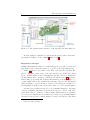


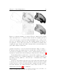


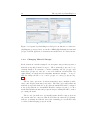

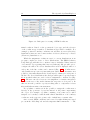


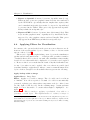


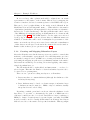




![[U2.04.01] Conseils d`utilisation de STAT_NON_LINE](http://vs1.manualzilla.com/store/data/006387325_1-7ad4067d146d4f613a19a506212e55bf-150x150.png)