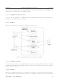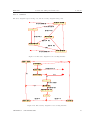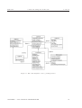
1
LIX, École Polytechnique Software Modelling and Architecture: Exercises Leo Liberti [email protected] Last update: October 22, 2008 Exercises Software Modelling and Architecture L. Liberti 2 Contents 1 Introduction 1.1 7 Structure of this book . . . . . . . . . . . . . . . . . . . . . . . . . . . . . . . . . . . . . . 2 UML exercises 2.1 2.2 2.3 2.4 9 Use case diagrams . . . . . . . . . . . . . . . . . . . . . . . . . . . . . . . . . . . . . . . . 9 2.1.1 Simplified ATM machine . . . . . . . . . . . . . . . . . . . . . . . . . . . . . . . . 10 2.1.2 Vending machine . . . . . . . . . . . . . . . . . . . . . . . . . . . . . . . . . . . . . 10 Sequence diagrams . . . . . . . . . . . . . . . . . . . . . . . . . . . . . . . . . . . . . . . . 12 2.2.1 The norm of a vector . . . . . . . . . . . . . . . . . . . . . . . . . . . . . . . . . . . 12 2.2.2 Displaying graphical objects . . . . . . . . . . . . . . . . . . . . . . . . . . . . . . . 13 2.2.3 Vending machine . . . . . . . . . . . . . . . . . . . . . . . . . . . . . . . . . . . . . 14 2.2.4 Boy/girl interaction . . . . . . . . . . . . . . . . . . . . . . . . . . . . . . . . . . . 15 State diagrams . . . . . . . . . . . . . . . . . . . . . . . . . . . . . . . . . . . . . . . . . . 15 2.3.1 Vending machine . . . . . . . . . . . . . . . . . . . . . . . . . . . . . . . . . . . . . 16 Class diagrams . . . . . . . . . . . . . . . . . . . . . . . . . . . . . . . . . . . . . . . . . . 18 2.4.1 Complex number class . . . . . . . . . . . . . . . . . . . . . . . . . . . . . . . . . . 18 2.4.2 Singly linked list . . . . . . . . . . . . . . . . . . . . . . . . . . . . . . . . . . . . . 23 2.4.3 Doubly linked list . . . . . . . . . . . . . . . . . . . . . . . . . . . . . . . . . . . . 23 2.4.4 Binary tree . . . . . . . . . . . . . . . . . . . . . . . . . . . . . . . . . . . . . . . . 24 2.4.5 n-ary tree . . . . . . . . . . . . . . . . . . . . . . . . . . . . . . . . . . . . . . . . . 24 2.4.6 Vending machine . . . . . . . . . . . . . . . . . . . . . . . . . . . . . . . . . . . . . 25 3 Modelling 3.1 7 27 The vending machine revisited . . . . . . . . . . . . . . . . . . . . . . . . . . . . . . . . . 27 3.1.1 27 Solution . . . . . . . . . . . . . . . . . . . . . . . . . . . . . . . . . . . . . . . . . . 3 Software Modelling and Architecture Exercises 3.2 L. Liberti Mistakes in modelling a tree . . . . . . . . . . . . . . . . . . . . . . . . . . . . . . . . . . . 27 3.2.1 31 Solution . . . . . . . . . . . . . . . . . . . . . . . . . . . . . . . . . . . . . . . . . . 4 Mathematical programming exercises 4.1 4.2 4.3 4.4 4.5 4.6 33 Museum guards . . . . . . . . . . . . . . . . . . . . . . . . . . . . . . . . . . . . . . . . . . 33 4.1.1 Solution . . . . . . . . . . . . . . . . . . . . . . . . . . . . . . . . . . . . . . . . . . 34 Mixed production . . . . . . . . . . . . . . . . . . . . . . . . . . . . . . . . . . . . . . . . . 36 4.2.1 Solution . . . . . . . . . . . . . . . . . . . . . . . . . . . . . . . . . . . . . . . . . . 36 Checksum . . . . . . . . . . . . . . . . . . . . . . . . . . . . . . . . . . . . . . . . . . . . . 38 4.3.1 Solution . . . . . . . . . . . . . . . . . . . . . . . . . . . . . . . . . . . . . . . . . . 40 Network Design . . . . . . . . . . . . . . . . . . . . . . . . . . . . . . . . . . . . . . . . . . 43 4.4.1 Solution . . . . . . . . . . . . . . . . . . . . . . . . . . . . . . . . . . . . . . . . . . 44 Error correcting codes . . . . . . . . . . . . . . . . . . . . . . . . . . . . . . . . . . . . . . 47 4.5.1 Solution . . . . . . . . . . . . . . . . . . . . . . . . . . . . . . . . . . . . . . . . . . 47 Selection of software components . . . . . . . . . . . . . . . . . . . . . . . . . . . . . . . . 48 4.6.1 48 Solution . . . . . . . . . . . . . . . . . . . . . . . . . . . . . . . . . . . . . . . . . . 5 Log analysis architecture 51 5.1 Definitions . . . . . . . . . . . . . . . . . . . . . . . . . . . . . . . . . . . . . . . . . . . . . 51 5.2 Software goals . . . . . . . . . . . . . . . . . . . . . . . . . . . . . . . . . . . . . . . . . . . 51 5.3 Requirements . . . . . . . . . . . . . . . . . . . . . . . . . . . . . . . . . . . . . . . . . . . 52 5.3.1 User interaction . . . . . . . . . . . . . . . . . . . . . . . . . . . . . . . . . . . . . 52 5.3.2 Log file reading . . . . . . . . . . . . . . . . . . . . . . . . . . . . . . . . . . . . . . 52 5.3.3 Computation and statistics . . . . . . . . . . . . . . . . . . . . . . . . . . . . . . . 52 The software architecture . . . . . . . . . . . . . . . . . . . . . . . . . . . . . . . . . . . . 52 5.4.1 Summary . . . . . . . . . . . . . . . . . . . . . . . . . . . . . . . . . . . . . . . . . 53 5.4.2 Details . . . . . . . . . . . . . . . . . . . . . . . . . . . . . . . . . . . . . . . . . . . 55 5.4 6 A search engine for projects 61 6.1 The setting . . . . . . . . . . . . . . . . . . . . . . . . . . . . . . . . . . . . . . . . . . . . 61 6.2 Initial offer . . . . . . . . . . . . . . . . . . . . . . . . . . . . . . . . . . . . . . . . . . . . 62 6.2.1 Kick-off meeting . . . . . . . . . . . . . . . . . . . . . . . . . . . . . . . . . . . . . 62 6.2.2 Brainstorming meeting . . . . . . . . . . . . . . . . . . . . . . . . . . . . . . . . . . 63 CONTENTS 4 Exercises 6.2.3 6.3 Software Modelling and Architecture L. Liberti Formalization of a commercial offer . . . . . . . . . . . . . . . . . . . . . . . . . . . 65 System planning . . . . . . . . . . . . . . . . . . . . . . . . . . . . . . . . . . . . . . . . . 67 6.3.1 Understanding T-Sale’s database structure . . . . . . . . . . . . . . . . . . . . . . 67 6.3.2 Brainstorming: Ideas proposal . . . . . . . . . . . . . . . . . . . . . . . . . . . . . 69 6.3.3 Functional architecture . . . . . . . . . . . . . . . . . . . . . . . . . . . . . . . . . 70 6.3.4 Technical architecture . . . . . . . . . . . . . . . . . . . . . . . . . . . . . . . . . . 78 CONTENTS 5 Exercises CONTENTS Software Modelling and Architecture L. Liberti 6 Chapter 1 Introduction This exercise book is meant to go with the course on Software Modelling given at École Polytechnique by Prof. D. Krob — the current course edition is 1st semester 2008/2009 (code INF556). This book contains a set of exercises in software modelling and architecture. 1.1 Structure of this book Software modelling and software architecture are concepts needed when planning complex software systems. The book will focus on exercises to be carried out by means of the UML language, some notions of optimization, and a good deal of common sense. One becomes a good software architect by experience. Chapter 2 focuses on simple UML exercises. It is split in Sections 2.1 (use case diagrams), 2.2 (sequence diagrams), 2.3 (state diagrams) and 2.4 (class diagrams). Chapter 3 groups various modelling exercises, only some of which involve UML. Chapters 5 and 6 are “large scale exercises” that should give meaningful examples on various modelling techniques used in practical settings (these sometimes employ UMLlike diagrams, but are not necessarily based on UML). Since some of these exercises use mathematical programming techniques, there is a small collection of exercises on mathematical programming in Chapter 4. 7 Exercises Software Modelling and Architecture CHAPTER 1. INTRODUCTION L. Liberti 8 Chapter 2 UML exercises This chapter proposes small to medium scale exercises on UML. Some of them are by the author, whilst others have been taken from books (credits are made explicit in each exercise: where no explicit citation is given, the exercise is to be considered the author’s work). UML is a graphical language consisting of diagrams of many different types, each referring to a system (be it a software system or otherwise) seen from a specific point of view. Thus, use case diagrams illustrate actors and actions of a system without any reference to logic or the temporal sequence of events; sequence diagrams underline the temporal event flow; state diagrams encode the logical relations among system components; class diagrams are used to represent the system organization into blocks each of which includes data and actions relative to those data. Of these diagrams, the former two (use case and sequence diagrams) are not considered as formal languages but rather as an aid tool to thought and system organization. The latter (state and class) can be considered as formal languages, although, really, compilers exist mostly just for class diagrams (taking a graphical description and outputting corresponding C++ or Java header files). Students should therefore aim at clarity for what concerns use case and sequence diagram and at formal rigourousness for state and (especially) class diagrams. UML diagrams can be used as a tool in system design. One usually starts with the simplest type of diagram, i.e. use case diagrams, to make sure the understanding of actors and actions of the system is clear. One then proceeds to sequence diagrams, adding a temporal scale to the system events. Next come state diagrams and finally the closest software representation of the system, the class diagram (there are more than four types of UML diagrams but in this book we shall limit ourselves to these four types). Each step is likely to underline system design errors in previous steps, so that the whole process is a continuous backtrack through use case, sequence, state and class diagrams so that in the end the whole diagram set presents a consistent system picture. Do not eschew backtracking, correcting and re-thinking current diagrams, for this is one of the main system design values added by UML. The student’s approach should absolutely not be “it took me three hours to put together the use case diagram and several days to compose sequence and state diagrams; and now I’m certainly NOT going to change it just because of one small inconsistency in the class diagram, which is likely to require me to change the whole thing”. Usually, one small inconsistency in the class diagram is all it takes for the whole system organization to fall apart. The point is that without UML the error would have gone unnoticed and likely crept in the system implementation, with catastrophic consequences. 2.1 Use case diagrams In this section we give some examples of use case diagrams for various situations. In general use case diagrams consists of a system (represented by a large box), actors (represented by small stylized men out 9 Software Modelling and Architecture Exercises L. Liberti of the box), actions (represented by ellipses within the box) and relations (edges or arcs linking actors with actions, actors with actors, actions with actions). 2.1.1 Simplified ATM machine Propose a use case diagram for an ATM machine for withdrawing cash. Make the use case simple yet informative; only include the major features. 2.1.1.1 Solution The use case diagram is given in Fig. 2.1 (taken from [7], Fig. 16.5). Figure 2.1: The simplified use case diagram of an ATM. 2.1.2 Vending machine Propose a use case diagram for a vending machine that sells beverages and snacks. Make use of inclusion and extension associations, mark multiplicities and remember that a vending machine may need technical assistance from time to time. 2.1.2.1 Solution The use case diagram is given in Fig. 2.2. The symbols at each end of relation edges are called multiplicities, and they indicate how many times a given action occurs linked to its actor(s), and how many times a CHAPTER 2. UML EXERCISES 10 Software Modelling and Architecture Exercises L. Liberti given actor carries out the corresponding actions; a multiplicity n..∗ next to an action indicates that the actor can carry it out a minimum of n times and a maximum of ∞ times. Boxes carrying a binary logical operator label (and, or, xor) help inserting some logical meaining into a use case diagram. A relation (A, B) carrying a triangle-shaped arrowhead next to B stands for generalization: object (actor or action) B generalises object A, which means that A has all the properties of B and some more (thus, an “angry client” is a client with one more property, that of being angry — an angry client can thus carry out all the actions that can be carried out by any client, plus some more relative to his/her added properties). A dashed action-action relation (A, B) carrying a label “include” means that action B necessarily takes place within action A. For example, confirming that we want to buy a good necessarily includes retrieving that good — although one might imagine a case of somebody using the machine in a train station and abandoning the good (already paid for) because the train is about to leave, the “train” element is evidently completely removed from the “vending machine” system, and so need not be modelled. A dashed action-action relation (A, B) carrying the label “extends” means that action A may take place within action B (notice that this relation is reversed with respect to the “include” relation). For example, once we confirm we want to buy some good, we necessarily retrieve the good but there may be no change to collect. Vending machine choose beverage choose good +1 include include input code looking input coin +1..* +1 +1 +0..1 confirm +1 client choose snack {xor} +0..1 +1 +1 cancel extends include include assistance operator (secondary) +1 retrieve coins retrieve good {xor} +0..1 +0..1 angry client +1 fix machine call assistance +0..* kick machine extend refill extend fix Figure 2.2: The use case diagram of a vending machine. CHAPTER 2. UML EXERCISES 11 Software Modelling and Architecture Exercises 2.2 L. Liberti Sequence diagrams In this section we shall present some easy examples of sequence diagrams. These are similar to twodimensional Euclidean planes, the horizontal axis marking labels for a finite set of actors and system components, and the (downward) vertical axis representing time. Actors and components are usually derived from a use case diagram. Actions are split into messages going back and forth between actors and components. Messages are represented by horizontal arrows. There are two types of messages: synchronous (the initiator of the message is blocked until a return value is sent back from the message recipient) and asynchronous (the initiator is not blocked and any return value must be carried by a later message where the initiator is the recipient of the asynchronous message). 2.2.1 The norm of a vector Consider the following algorithm for computing the norm of a vector. Class Array { ... public: // return the size of the array int size(void); // return the index-th component of the array double get(int index); ... }; double norm(const Array& myArray) { double theNorm = 0; double c = 0; for(int index = 0; index < myArray.size() - 1; index++) { c = myArray.get(index); theNorm = theNorm + c*c; } theNorm = sqrt(theNorm); return theNorm; } Write down a sequence diagram illustrating the behaviour of the norm() function. 2.2.1.1 Solution In order to draw a sequence diagram we must first draw a use case diagram to help us identify system, actors and actions. In this case, drawing a use case diagram is not all that simple: we have a static piece of code. Where is the system? Who are the actors? It turns out that the code has a class and a function outside the class. In this setting, the class is passive. If no entity calls the class methods, the class will not carry out any action of its own accord. The class is therefore to be considered as a system rather than an actor. The norm() function, on the other hand, calls methods within the class, and can thus be likened to an actor. The actions are precisely those methods that are called by norm(). This arrangement is shown in Fig. 2.3 Having identified actors, actions and system, we can now build the sequence diagram. The norm() function calls two Array methods: size() and get(), both of which block norm() until a return value CHAPTER 2. UML EXERCISES 12 Software Modelling and Architecture Exercises L. Liberti class Array size() norm() get(int) Figure 2.3: The use case diagram of the norm()/Array system. is received (and can therefore be represented by asynchronous messages). One other notable non-local action carried out by norm() is the call to the sqrt() method. This is external to norm() so it should be represented on the sequence diagram; on the other hand, we have no system component where sqrt() belongs — in practice, the function sqrt() is found in a system library called libm on UNIX systems, but this is hardly part of the system at hand so it has no representation. In such cases, we depict the sqrt() call as a self-action of the norm() actor onto itself. This is shown in Fig. 2.4. : norm() : array 1: size() 2: get(index) 3: sqrt() Figure 2.4: The sequence diagram describing the computation of the norm of a vector. 2.2.2 Displaying graphical objects Write a sequence diagram for a program that displays Fig. 2.5 on the screen in the order left → right. CHAPTER 2. UML EXERCISES 13 Software Modelling and Architecture Exercises L. Liberti Figure 2.5: 2.2.2.1 Solution The sequence diagram in Fig. 2.6 describes the required behaviour. Figure 2.6: The sequence diagram describing the printing of the drawing in Fig. 2.5. 2.2.3 Vending machine Draw a sequence diagram for the vending machine of Sect. 2.1.2. 2.2.3.1 Solution The sequence diagram in Fig. 2.7 describes the required behaviour. Notice the box-shaped elements in the diagram: these are used to endow the diagram with a modicum of logical representation: alt signals an alternative (an if. . . else block), opt signals an option (an if block) and loop a loop (a for or while block). CHAPTER 2. UML EXERCISES 14 Software Modelling and Architecture Exercises L. Liberti Figure 2.7: The sequence diagram for the vending machine of Sect. 2.1.2. 2.2.4 Boy/girl interaction A boy takes a fancy to a girl, and wants her to become his girlfriend. Draw a sequence diagram for their interactions (to avoid any accusation of genderwise discrimination, you can also reverse the roles of boy and girl). 2.2.4.1 Solution The sequence diagram in Fig. 2.8 illustrates the interactions between boy and girl. Some other actors and system components have been added, mostly for fun. 2.3 State diagrams In this section we present some elementary exercises on state diagrams. State diagrams are similar to state automata, and are used to describe the logic behind any state change within a system or a system component. States are represented by rounded-corner boxes with a label (the state name); a change from CHAPTER 2. UML EXERCISES 15 Software Modelling and Architecture Exercises L. Liberti : girl's "agony aunt" friend : other boy : boy : girl : girl's father 1: see() loop for a very long time 2: talk() "get lost, creep" 3: flirt smooch 4: threaten_father_call "but I love you" par 5: boy_call par 5: daddy_call 6: get_up_from_couch 6: bash_to_pulp 6: bash_to_pulp 7: ask_judgment "nah, you did well, he's a creep" 8: notice_vulnerable_pulp 9: feel_mothering_instinct 10: express_love "'had enough, fuck you" 11: ask_comfort "all men are bastards" Figure 2.8: The sequence diagram for the boy/girl interactions. state A to state B is represented by an arrow from A to B. Two types of states, “start” and “end”, are such that there are no incoming arrows into “start” and no outgoing arrows from “end” states. Arrows are labelled by the name of the activity that caused the state change. Another type of state diagram, called activity diagram, emphasizes activities rather than states: activity names label the round-cornered boxes, and the state names label the arrows. Apart from “start” and “end” nodes, activity diagrams also have special “test” nodes represented by small rhombi. 2.3.1 Vending machine Draw state and activity diagrams for the vending machine described in Sections 2.1.2 and 2.2.3. CHAPTER 2. UML EXERCISES 16 Software Modelling and Architecture Exercises 2.3.1.1 L. Liberti Solution The state diagram is given in Fig. 2.9, and the activity diagram in Fig. 2.10. operator switches on waiting for selection user selects good displaying cost money = cost money < cost delivering good money >= cost waiting for money money > cost abort delivering change operator switches off Figure 2.9: The state diagram for the vending machine. change < money deliver change selfdiagnostic tests machine ready yes verify "off" control no yes wait for selection user selects product no wait for money user inputs money change = money cost check change check for abort change < 0 change >= 0 deliver good Figure 2.10: The activity diagram for the vending machine. CHAPTER 2. UML EXERCISES 17 Software Modelling and Architecture Exercises 2.4 L. Liberti Class diagrams In this section we present some elementary exercises on class diagrams. 2.4.1 Complex number class Draw a class diagram for the single class Complex. A Complex object has a private real and an imaginary part (of type double), and can perform addition, subtraction, multiplication and division by another complex number. 2.4.1.1 Solution The class diagram for the Complex class is given in Fig. 2.11. Complex realPart : double = 0 imaginaryPart : double = 0 + setReal(theRealPart : double) + setImaginary(theImaginaryPart : double) + getReal() : double + getImaginary() : double + absoluteValue() : double + add(theComplexNumber : Complex) + subtract(theComplexNumber : Complex) + multiplyBy(theComplexNumber : Complex) + divideBy(theComplexNumber : Complex) Figure 2.11: The class diagram for a complex number. Most UML modellers can be used to automatically generate C++ (or Java) code from the class diagram. This results in “class skeleton” files (a header file Complex.h and a corresponding implementation file Complex.cpp). Both are given below. /************************************************************************ Complex.h.h - Copyright liberti Here you can write a license for your code, some comments or any other information you want to have in your generated code. To to this simply configure the "headings" directory in uml to point to a directory where you have your heading files. or you can just replace the contents of this file with your own. If you want to do this, this file is located at /usr/share/apps/umbrello/headings/heading.h -->Code Generators searches for heading files based on the file extension i.e. it will look for a file name ending in ".h" to include in C++ header files, and for a file name ending in ".java" to include in all generated java code. If you name the file "heading.<extension>", Code Generator will always choose this file even if there are other files with the same extension in the directory. If you name the file something else, it must be the only one with that extension in the directory to guarantee that Code Generator will choose it. you can use variables in your heading files which are replaced at generation CHAPTER 2. UML EXERCISES 18 Exercises Software Modelling and Architecture L. Liberti time. possible variables are : author, date, time, filename and filepath. just write %variable_name% This file was generated on %date% at %time% **************************************************************************/ #ifndef COMPLEX_H #define COMPLEX_H #include <string> /** * class Complex */ class Complex { public: // Constructors/Destructors // /** * Empty Constructor */ Complex ( ); /** * Empty Destructor */ virtual ~Complex ( ); // Static public attributes // // public attributes // // public attribute accessor methods // // public attribute accessor methods // /** * @param theRealPart */ void setReal (double theRealPart ); /** * @param theImaginaryPart */ void setImaginary (double theImaginaryPart ); /** * @return double */ double getReal ( ); /** * @return double */ double getImaginary ( ); /** * @return double */ double absoluteValue ( ); /** CHAPTER 2. UML EXERCISES 19 Exercises Software Modelling and Architecture L. Liberti * @param theComplexNumber */ void add (Complex theComplexNumber ); /** * @param theComplexNumber */ void subtract (Complex theComplexNumber ); /** * @param theComplexNumber */ void multiplyBy (Complex theComplexNumber ); /** * @param theComplexNumber */ void divideBy (Complex theComplexNumber ); protected: // Static protected attributes // // protected attributes // public: // protected attribute accessor methods // protected: public: // protected attribute accessor methods // protected: private: // Static private attributes // // private attributes // double m_realPart; double m_imaginaryPart; public: // private attribute accessor methods // private: public: // private attribute accessor methods // /** * Set the value of m_realPart * @param new_var the new value of m_realPart */ void setRealPart ( double new_var ); /** * Get the value of m_realPart * @return the value of m_realPart CHAPTER 2. UML EXERCISES 20 Exercises Software Modelling and Architecture L. Liberti */ double getRealPart ( ); /** * Set the value of m_imaginaryPart * @param new_var the new value of m_imaginaryPart */ void setImaginaryPart ( double new_var ); /** * Get the value of m_imaginaryPart * @return the value of m_imaginaryPart */ double getImaginaryPart ( ); private: void initAttributes ( ) ; }; #endif // COMPLEX_H /************************************************************************ Complex.h.cpp - Copyright liberti Here you can write a license for your code, some comments or any other information you want to have in your generated code. To to this simply configure the "headings" directory in uml to point to a directory where you have your heading files. or you can just replace the contents of this file with your own. If you want to do this, this file is located at /usr/share/apps/umbrello/headings/heading.cpp -->Code Generators searches for heading files based on the file extension i.e. it will look for a file name ending in ".h" to include in C++ header files, and for a file name ending in ".java" to include in all generated java code. If you name the file "heading.<extension>", Code Generator will always choose this file even if there are other files with the same extension in the directory. If you name the file something else, it must be the only one with that extension in the directory to guarantee that Code Generator will choose it. you can use variables in your heading files which are replaced at generation time. possible variables are : author, date, time, filename and filepath. just write %variable_name% This file was generated on %date% at %time% **************************************************************************/ #include "Complex.h" // Constructors/Destructors // Complex::Complex ( ) { initAttributes(); } Complex::~Complex ( ) { } // // Methods // // Accessor methods // // public static attribute accessor methods // // public attribute accessor methods // CHAPTER 2. UML EXERCISES 21 Exercises Software Modelling and Architecture L. Liberti // protected static attribute accessor methods // // protected attribute accessor methods // // private static attribute accessor methods // // private attribute accessor methods // /** * Set the value of m_realPart * @param new_var the new value of m_realPart */ void Complex::setRealPart ( double new_var ) { m_realPart = new_var; } /** * Get the value of m_realPart * @return the value of m_realPart */ double Complex::getRealPart ( ) { return m_realPart; } /** * Set the value of m_imaginaryPart * @param new_var the new value of m_imaginaryPart */ void Complex::setImaginaryPart ( double new_var ) { m_imaginaryPart = new_var; } /** * Get the value of m_imaginaryPart * @return the value of m_imaginaryPart */ double Complex::getImaginaryPart ( ) { return m_imaginaryPart; } // Other methods // /** * @param theRealPart */ void Complex::setReal (double theRealPart ) { } /** * @param theImaginaryPart */ void Complex::setImaginary (double theImaginaryPart ) { } /** * @return double */ double Complex::getReal ( ) { } /** * @return double */ CHAPTER 2. UML EXERCISES 22 Software Modelling and Architecture Exercises L. Liberti double Complex::getImaginary ( ) { } /** * @return double */ double Complex::absoluteValue ( ) { } /** * @param theComplexNumber */ void Complex::add (Complex theComplexNumber ) { } /** * @param theComplexNumber */ void Complex::subtract (Complex theComplexNumber ) { } /** * @param theComplexNumber */ void Complex::multiplyBy (Complex theComplexNumber ) { } /** * @param theComplexNumber */ void Complex::divideBy (Complex theComplexNumber ) { } void Complex::initAttributes ( ) { m_realPart = 0; m_imaginaryPart = 0; } 2.4.2 Singly linked list Draw a class diagram representing a singly linked list. 2.4.2.1 Solution The class diagram is given in Fig. 2.12. It consists of a class with a single unidirectional association (next) with multiplicity 1, because a node of a singly linked list only has one neighbouring node (the next node). 2.4.3 Doubly linked list Draw a class diagram representing a doubly linked list. CHAPTER 2. UML EXERCISES 23 Software Modelling and Architecture Exercises L. Liberti 1 +next slList Figure 2.12: The class diagram of a singly linked list. 2.4.3.1 Solution The class diagram is given in Fig. 2.13. It consists of a class with a single bidirectional association with reference names previous and next both with multiplicity 1, because a doubly linked list has a previous and a next node. +previous 1 dlList +next 1 Figure 2.13: The class diagram of a doubly linked list. 2.4.4 Binary tree Draw a class diagram representing a binary tree. 2.4.4.1 Solution The class diagram is given in Fig. 2.14. It consists of a class with a single bidirectional association with reference names child (with multiplicity 2) and parent (with multiplicity 1), because a binary tree has two children and one parent node. +parent 1 node 2 +child Figure 2.14: The class diagram of a binary tree. 2.4.5 n-ary tree Draw a class diagram representing an n-ary tree (a tree with a variable number of children nodes). CHAPTER 2. UML EXERCISES 24 Software Modelling and Architecture Exercises 2.4.5.1 L. Liberti Solution The class diagram is given in Fig. 2.15. It consists of a class with a single bidirectional association with reference names child (with multiplicity ∗) and parent (with multiplicity 1), because a binary tree has a variable number of children and one parent node. +parent 1 node * +child Figure 2.15: The class diagram of an n-ary tree. 2.4.6 Vending machine Draw a class diagram for the vending machine described in Sect. 2.1.2 and 2.2.3. 2.4.6.1 Solution The class diagram is given in Fig. 2.16. VendingMachine goods : Inventory Client coins : Inventory + chooseGood(theGood : ) + inputCoin(theMoney : ) + confirm() + askSelection(theCode : ) * 1..* use + askMoney(theMoney : ) +c lVendingMac hine +vmClient + askConfirmation() + cancel() + askCallAssistance() + retrieveGood(theGood : ) + callAssistance(theTrouble : int) + callAssistance() + isGoodAvailable(theGood : ) + isChangeAvailable(theMoney : ) +aoVendingMac hine 1..* c oins goods Inventory fix 1..* +vmAssistanc eOp AssistanceOperator +previous type : 1 number : 1 +next + fix() AngryClient + refill(theGood : ) + kickMachine() Figure 2.16: The class diagram of a vending machine. CHAPTER 2. UML EXERCISES 25 Exercises Software Modelling and Architecture CHAPTER 2. UML EXERCISES L. Liberti 26 Chapter 3 Modelling This chapter groups some modelling exercises, only some of which involve UML. 3.1 The vending machine revisited Consider the vending machine described in Sect. 2.1.2, 2.2.3 and 2.4.6. The proposed use case diagram (Fig. 2.2), sequence diagram (Fig. 2.7) and class diagram (Fig. 2.16) make up for a very poor system modelling indeed. The vending machine is always thought of as a monolitic entity: this makes the external relationships clear but says nothing about how to plan and build one. In particular, the monolitic view is incompatible with the fact that a vending machine is composed of different parts. Given the following list of parts: 1. main controller 2. mechanical robot 3. coin acceptor 4. remote messaging system 5. door and the fact that 2,3,4,5 can only be interfaced with 1, draw a use case diagram and a sequence diagram to provide an initial blueprint for the inner workings of a vending machine. 3.1.1 Solution The use case diagram is found in Fig. 3.1. The sequence diagram is found in Fig. 3.2. Notice that they do not provide mechanisms for calling assistance operators on failure of providing change and/or food. How should these diagrams change to cater for these occurrences? 3.2 Mistakes in modelling a tree Fig. 3.3 describes the class diagram of a tree node, which can be used recursively to build an expression tree. 27 Software Modelling and Architecture Exercises ask for money ask good selection L. Liberti verify good availability ask confirmation main controller select good output good call assistance mechanical robot run system tests input money output money confirm deal out good remote messaging system send message to assistance return money coin acceptor retrieve good call help customer accept money open door refill assistance operator Figure 3.1: The revised use case diagram of the vending machine. Generate the header file and implementation code using Umbrello, then add the implementation of the only non-obvious functions (getNumberOfChildren and getChildType) as follows: int TreeNode::getNumberOfChildren ( ) { // number of children int nc = 0; switch(m_operatorLabel) { case 0: // sum nc = 2; break; case 1: // difference nc = 2; break; case 2: // multiplication nc = 2; break; case 3: // division nc = 2; break; case 4: // square nc = 1; break; case 5: // cube nc = 1; break; CHAPTER 3. MODELLING 28 Software Modelling and Architecture Exercises : AssistanceOp : Customer : Controller : Robot : CoinAcceptor L. Liberti : MessagingSystem : Door : selectGood(theGood) : verifyAvailability(theGood) : bool : callAssistance(problemType):bool if not available : assistanceRefill() : openAndRefill() : updateInventory repeat : displayOutstanding(theMoney) : insertMoney(theMoney) : newAmount() : getAmount():int until amount < price : confirmOrCancel(): bool if confirmed : outProduct(theProduct) : dealProduct(theProduct) : outputChange(theMoney) : takeGood(theGood) Figure 3.2: The revised sequence diagram of a vending machine. TreeNode operatorLabel : int = 0 level : int = 0 leftChild : TreeNodePtr rightChild : TreeNodePtr + getNumberOfChildren() : int + getChildType(childIndex : int = 0, theChildLevel : int = 0) : int +leftChild +rightChild «datatype» TreeNodePtr Figure 3.3: The UML class diagram for the TreeNode class. case 6: // sqrt nc = 1; break; case 10: // number nc = 0; break; default: break; CHAPTER 3. MODELLING 29 Exercises Software Modelling and Architecture L. Liberti } return nc; } int TreeNode::getChildType (int childIndex, int theChildLevel) { int ret = -1; // increase the level by one unit theChildLevel++; if (childIndex == 0) { // left child ret = m_leftChild->getOperatorLabel(); } else if (childIndex == 1) { // right child ret = m_rightChild->getOperatorLabel(); } return ret; } Now consider the following main function in the file TreeNode main.cxx: // TreeNode_main.cxx #include <iostream> #include "TreeNode.h" int main(int argc, char** argv) { int ret = 0; // expression tree t: number + number^2 TreeNode t; t.setOperatorLabel(0); t.setLevel(0); t.setLeftChild(new TreeNode); t.setRightChild(new TreeNode); t.getLeftChild()->setOperatorLabel(10); t.getLeftChild()->setLevel(1); t.getRightChild()->setOperatorLabel(4); t.getRightChild()->setLevel(1); t.getRightChild()->setLeftChild(new TreeNode); t.getRightChild()->getLeftChild()->setOperatorLabel(10); t.getRightChild()->getLeftChild()->setLevel(2); // get right child type and level int theLevel = 0; int theOperatorLabel = -1; theOperatorLabel = t.getChildType(1, theLevel); // expect theOperatorLabel = 4, theLevel = 1; std::cout << theOperatorLabel << ", " << theLevel << std::endl; // actual output is 4,0 return ret; } Compile the project by typing: c++ -o TreeNode TreeNode main.cxx TreeNode.cpp CHAPTER 3. MODELLING 30 Software Modelling and Architecture Exercises L. Liberti and verify whether the output is as expected (4, 1). If not, why? Is this a bug or a modelling error? We would now like to code in TreeNode main.cxx a new function that accepts a tree node and returns the number of children of the root node of the expression tree. Convince yourself that you cannot do this easily, and explain why. How can you fix this modelling error? Change the UML diagram and the code accordingly. 3.2.1 Solution The output is 4, 0. The problem is given by the fact that the second argument of getChildType, that is, theLevel, was not declared as an inout (read/write) parameter but as an in (read only) parameter instead, so it cannot be changed by the function itself (notice the compiler issues no warning about this occurrence: it is perfectly legal syntactically if not semantically). The new function cannot be coded in because the model provide no mechanism for going from a given node to its parent node, much less the root node of the tree. The correct UML class diagram is given in Fig. 3.4. TreeNode operatorLabel : int = 0 level : int = 0 leftChild : TreeNodePtr rightChild : TreeNodePtr parent : TreeNodePtr + getNumberOfChildren() : int + getChildType(childIndex : int = 0, theChildLevel : int = 0) : int +leftChild parent +rightChild «datatype» TreeNodePtr Figure 3.4: The corrected UML class diagram for the TreeNode class. CHAPTER 3. MODELLING 31 Exercises CHAPTER 3. MODELLING Software Modelling and Architecture L. Liberti 32 Chapter 4 Mathematical programming exercises The mathematical programming formulation language is a very powerful tool used to formalize optimization problems by means of parameters, decision variables, objective functions and constraints. Such diverse settings as combinatorial, integer, continuous, linear and nonlinear optimization problems can be defined precisely by their corresponding mathematical programming formulations. Its power is not limited to its expressiveness, but usually allows hassle-free solution of the problem: most general-purpose solution algorithms solve optimization problems cast in their mathematical programming formulation, and the corresponding implementations can usually be hooked into language environments which allow the user to input and solve complex optimization problems easily. This chapter provides an introduction (by way of examples) to a mathematical programming software system, called AMPL (A Mathematical Programming Language) [6] which is interfaced with continuous mixed-integer linear (CPLEX [8]) and nonlinear solvers. See www.ampl.com for details on downloading and installing the student versions of AMPL and CPLEX. 4.1 Museum guards A museum director must decide how many guards should be employed to control a new wing. Budget cuts have forced him to station guards at each door, guarding two rooms at once. Formulate a mathematical program to minimize the number of guards. Solve the problem on the map below using AMPL. J I E F G H B D A C Also solve the problem on the following map. 33 Software Modelling and Architecture Exercises S R Q L N M H J G K T P O D A Z Y I W U X L. Liberti C E B F [P. Belotti, Carnegie Mellon University] 4.1.1 Solution The problem can be formalized by representing each museum room by a vertex v ∈ V of an undirected graph G = (V, E). There is an edge between two vertices if there is a door leading from one room to the other; this way, edges represent the possibility of there being a guard on a door. We want to choose the smallest subset F ⊆ E of edges covering all vertices, i.e. such that for all v ∈ V there is w ∈ V with {v, w} ∈ F . J I E J D H B E F G H I G F D A C B A C To each {i, j} ∈ E we associated a binary variable xij is assigned the value 1 if there is a guard on the door represented by edge {i, j} and 0 otherwise. 4.1.1.1 Formulation • Parameters. G = (V, A): graph description of the museum topology. • Variables. xij : 1 if edge {i, j} ∈ E is to be included in F , 0 otherwise. • Objective function min X xij {i,j}∈E • Constraints. (Vertex cover): P xij ≥ 1 ∀i ∈ V . j∈V :{i,j}∈E CHAPTER 4. MATHEMATICAL PROGRAMMING EXERCISES 34 Software Modelling and Architecture Exercises 4.1.1.2 L. Liberti AMPL model, data, run # museum.mod param n >= 0, integer; set V := 1..n; set E within {V,V}; var x{E} binary; minimize cost : sum{(i,j) in E} x[i,j]; subject to vertexcover {i in V} : sum{j in V : (i,j) in E} x[i,j] + sum{j in V : (j,i) in E} x[j,i] >= 1; # museum.dat param n := 10; set E := 1 2 1 3 1 6 1 7 2 8 3 4 4 5 7 9 8 9 9 10 ; # museum.run model museum.mod; data museum.dat; option solver cplexstudent; solve; display cost; display x; 4.1.1.3 CPLEX solution CPLEX 7.1.0: optimal integer solution; objective 6 2 MIP simplex iterations 0 branch-and-bound nodes cost = 6 x 1 1 1 1 2 3 4 7 8 9 ; := 2 3 6 7 8 4 5 9 9 10 0 1 1 1 1 0 1 0 0 1 CHAPTER 4. MATHEMATICAL PROGRAMMING EXERCISES 35 Software Modelling and Architecture Exercises 4.2 L. Liberti Mixed production A firm is planning the production of 3 products A1 ,A2 ,A3 . In a month production can be active for 22 days. In the following tables are given: maximum demands (units=100kg), price ($/100Kg), production costs (per 100Kg of product), and production quotas (maximum amount of 100kg units of product that would be produced in a day if all production lines were dedicated to the product). Product Maximum demand Selling price Production cost Production quota A1 5300 $124 $73.30 500 A2 4500 $109 $52.90 450 A3 5400 $115 $65.40 550 1. Formulate an AMPL model to determine the production plan to maximize the total income. 2. Change the mathematical program and the AMPL model to cater for a fixed activation cost on the production line, as follows: Product Activation cost A1 $170000 A2 $150000 A3 $100000 3. Change the mathematical program and the AMPL model to cater for both the fixed activation cost and for a minimum production batch: Product Minimum batch A1 20 A2 20 A3 16 [E. Amaldi, Politecnico di Milano] 4.2.1 Solution 4.2.1.1 Formulation • Indicex: Let i be an index on the set {1, 2, 3}. • Parameters: – P : number of production days in a month; – di : maximum market demand for product i; – vi : selling price for product i; – ci : production cost for product i; – qi : maximum production quota for product i; – ai : activation cost for the plant producing i; – li : minimum batch of product i. • Variables: – xi : quantity of product i to produce (xi ≥ 0); – yi : activation status of product i (1 if active, 0 otherwise). CHAPTER 4. MATHEMATICAL PROGRAMMING EXERCISES 36 Software Modelling and Architecture Exercises L. Liberti • Objective function: max X ((vi − ci )xi − ai yi ) i • Constraints: 1. (demand): for each i, xi ≤ di ; P 2. (production): i xqii ≤ P ; 3. (activation): for each i, xi ≤ P qi yi ; 4. (minimum batch): for each i, xi ≥ li yi ; 4.2.1.2 AMPL model, data, run # mixedproduction.mod set PRODUCTS; param param param param param param param days >= 0; demand { PRODUCTS } >= 0; price { PRODUCTS } >= 0; cost { PRODUCTS } >= 0; quota { PRODUCTS } >= 0; activ_cost { PRODUCTS } >= 0; min_batch { PRODUCTS } >= 0; # activation costs # minimum batches var x { PRODUCTS } >= 0; var y { PRODUCTS } >= 0, binary; # quantity of product # activation of production lines maximize revenue: sum {i in PRODUCTS} ((price[i] - cost[i]) * x[i] - activ_cost[i] * y[i]); subject to requirement {i in PRODUCTS}: x[i] <= demand[i]; subject to production: sum {i in PRODUCTS} (x[i] / quota[i]) <= days; subject to activation {i in PRODUCTS}: x[i] <= days * quota[i] * y[i]; subject to batches {i in PRODUCTS}: x[i] >= min_batch[i] * y[i]; # mixedproduction.dat set PRODUCTS := A1 A2 A3 ; param days := 22; param : demand price A1 5300 124 A2 4500 109 A3 5400 115 cost quota 73.30 500 52.90 450 65.40 550 activ_cost min_batch := 170000 20 150000 20 100000 16 ; # mixedproduction.run CHAPTER 4. MATHEMATICAL PROGRAMMING EXERCISES 37 Software Modelling and Architecture Exercises L. Liberti model mixedproduction.mod; data mixedproduction.dat; option solver cplexstudent; solve; display x; display y; 4.2.1.3 CPLEX solution . CPLEX 7.1.0: optimal integer solution; objective 220690 5 MIP simplex iterations 0 branch-and-bound nodes ampl: display x; x [*] := A1 0 A2 4500 A3 5400 ; ampl: display y; y [*] := A1 0 A2 1 A3 1 ; 4.3 Checksum An expression parser is a program that reads mathematical expressions (input by the user as strings) and evaluates their values on a set of variable values. This is done by representing the mathematical expression as a directed binary tree. The leaf nodes represent variables or constants; the other nodes represent binary (or unary) operators such as arithmetic (+, -, *, /, power) or transcendental (sin, cos, tan, log, exp) operators. The unary operators are represented by a node with only one arc in its outgoing star, whereas the binary operators have two arcs. The figure below is the binary expression tree for (x + 2)ex . * 2 * + HH HH HH j H × HH x H H HH j H exp H H HH HH j x H CHAPTER 4. MATHEMATICAL PROGRAMMING EXERCISES 38 Exercises Software Modelling and Architecture L. Liberti The expression parser consists of several subroutines. • main(): the program entry point; • parse(): reads the string containing the mathematical expression and transforms it into a binary expression tree; • gettoken(): returns and deletes the next semantic token (variable, constant, operator, brackets) from the mathematical expression string buffer; • ungettoken(): pushes the current semantic token back in the mathematical expression string buffer; • readexpr(): reads the operators with precedence 4 (lowest: +,-); • readterm(): reads the operators with precedence 3 (*, /); • readpower(): reads the operators with precedence 2 (power); • readprimitive(): reads the operators of precedence 1 (functions, expressions in brackets); • sum(term a, term b): make a tree + ր ց a ; b • difference(term a, term b): make a tree − • product(term a, term b): make a tree ∗ ր ց • fraction(term a, term b): make a tree / • power(term a, term b): make a tree ∧ ր ց ր ց a ; b a ; b ր ց a ; b a ; b • minus(term a): make a tree − → a; • logarithm(term a): make a tree make a tree log → a; • exponential(term a): make a tree make a tree exp → a; • sine(term a): make a tree make a tree sin → a; • cosine(term a): make a tree make a tree cos → a; • tangent(term a): make a tree make a tree tan → a; • variable(var x): make a leaf node x; • number(double d): make a leaf node d; • readdata(): reads a table of variable values from a file; • evaluate(): computes the value of the binary tree when substituting each variable with the corresponding value; • printresult(): print the results. For each function we give the list of called functions and the quantity of data to be passed during the call. CHAPTER 4. MATHEMATICAL PROGRAMMING EXERCISES 39 Software Modelling and Architecture Exercises L. Liberti • main: readdata (64KB), parse (2KB), evaluate (66KB), printresult(64KB) • evaluate: evaluate (3KB) • parse: gettoken (0.1KB), readexpr (1KB) • readprimitive: gettoken (0.1KB), variable (0.5KB), number (0.2KB), logarithm (1KB), exponential (1KB), sine (1KB), cosine (1KB), tangent (1KB), minus (1KB), readexpr (2KB) • readpower: power (2KB), readprimitive (1KB) • readterm: readpower (2KB), product (2KB), fraction (2KB) • readexpr: readterm (2KB), sum (2KB), difference (2KB) • gettoken: ungettoken (0.1KB) Each function call requires a bidirectional data exchange between the calling and the called function. In order to guarantee data integrity during the function call, we require that a checksum operation be performed on the data exchanged between the pair (calling function, called function). Such pairs are called checksum pairs. Since the checksum operation is costly in terms of CPU time, we limit these operations so that no function may be involved in more than one checksum pair. Naturally though, we would like to maximize the total quantity of data undergoing a checksum. 1. Formulate a mathematical program to solve the problem, and solve the given instance with AMPL. 2. Modify the model to ensure that readprimitive() and readexpr() are a checksum pair. How does the solution change? 4.3.1 Solution We represent each subroutine with a vertex in an undirected graph G = (V, E). For each u, v ∈ V , {u, v} ∈ E if subroutine u calls subroutine v (or vice versa). Each edge {i, j} ∈ E is weighted by the quantity pij of data exchanged between the subroutines. We want to choose a subset L ⊆ E such that for each u ∈ V there is v ∈ V with {u, v} ∈ L (i.e. L covers V P ), such that each vertex v ∈ V is adjacent to exactly 1 edge in L and such that the total weight p(L) = {i,j}∈L pij is maximum. G is shown below. 0.1 gettoken 0.1 ungettoken 0.1 readdata variable 64 0.5 2 parse 1 main 66 0.2 number 3 2 64 evaluate readexpr printresult 2 2 2 readterm sum 2 2 1 1 readpower readprimitive 2 1 2 product power logarithm 1 exponential 1 sine difference fraction 1 cosine 1 tangent minus CHAPTER 4. MATHEMATICAL PROGRAMMING EXERCISES 40 Software Modelling and Architecture Exercises 4.3.1.1 L. Liberti Formulation • Parameters: for each {i, j} ∈ E, pij is the weight on the edge. • Variables: for each {i, j} ∈ E, xij = 1 if {i, j} ∈ L and 0 otherwise. • Objective function: max X pij xij e={i,j}∈E • Constraints: ∀i ∈ V X xij = 1; (4.1) j∈V |{i,j}∈E ∀{i, j} ∈ E 4.3.1.2 xij ∈ {0, 1}. (4.2) AMPL model, data, run # checksum.mod set V; set E within {V,V}; param p{E}; var x{E} binary; maximize data : sum{(i,j) in E} p[i,j] * x[i,j]; subject to assignment {i in V} : sum{j in V : (i,j) in E} x[i,j] + sum{j in V : (j,i) in E} x[j,i] <= 1; # checksum.dat set V := main readdata parse evaluate printresult gettoken readexpr readprimitive variable number logarithm exponential sine cosine tangent minus power readpower readterm product fraction sum ; set E := main readdata main parse main evaluate main printresult evaluate evaluate parse gettoken parse readexpr readprimitive gettoken readprimitive variable readprimitive number readprimitive logarithm readprimitive exponential readprimitive sine readprimitive cosine readprimitive tangent readprimitive minus readprimitive readexpr readpower power readpower readprimitive readterm readpower readterm product readterm fraction readexpr readterm CHAPTER 4. MATHEMATICAL PROGRAMMING EXERCISES 41 Software Modelling and Architecture Exercises readexpr sum L. Liberti ; param p := main readdata 64 main parse 2 main evaluate 66 main printresult 64 evaluate evaluate 3 parse gettoken 0.1 parse readexpr 1 readprimitive gettoken 0.1 readprimitive variable 0.5 readprimitive number 0.2 readprimitive logarithm 1 readprimitive exponential 1 readprimitive sine 1 readprimitive cosine 1 readprimitive tangent 1 readprimitive minus 1 readprimitive readexpr 2 readpower power 2 readpower readprimitive 1 readterm readpower 2 readterm product 2 readterm fraction 2 readexpr readterm 2 readexpr sum 2 ; # checksum.run model checksum.mod; data checksum.dat; option solver cplexstudent; solve; display data; printf "L = {\n"; for {(i,j) in E : x[i,j] = 1} { printf " (%s,%s)\n", i, j; } printf " }\n"; 4.3.1.3 CPLEX solution CPLEX 8.1.0: optimal integer solution; objective 73.1 3 MIP simplex iterations 0 branch-and-bound nodes data = 73.1 L = { (main,evaluate) (parse,gettoken) (readprimitive,cosine) (readpower,power) (readterm,product) (readexpr,sum) CHAPTER 4. MATHEMATICAL PROGRAMMING EXERCISES 42 Software Modelling and Architecture Exercises L. Liberti } The picture below is the solution represented on the graph. 0.1 gettoken 0.1 ungettoken 0.1 readdata variable 64 0.5 parse 2 1 main number 0.2 3 66 2 64 evaluate 2 2 readexpr printresult 2 2 readterm 2 readprimitive 2 1 1 2 sum logarithm 1 1 readpower power product exponential 1 sine difference 1 fraction cosine 1 tangent minus 4.4 Network Design Orange is the unique owner and handler of the telecom network in the figure below. 1 1.8 1 7 3 1.7 2 2 4 1 2 7 5 2 5.4 2 0.7 2.5 1 5 8 3 12 6 2 6.5 9 1.1 10 2.1 1.5 1 11 13 The costs on the links are proportional to the distances d(i, j) between the nodes, expressed in units of 10km. Because of anti-trust regulations, Orange must delegate to SFR and Bouygtel two subnetworks each having at least two nodes (with Orange handling the third part). Orange therefore needs to design a backbone network to connect the three subnetworks. Transforming an existing link into a backbone link costs c = 25 euros/km. Formulate a mathematical program to minimize the cost of implementing a backbone connecting the three subnetworks, and solve it with AMPL. How does the solution change if Orange decides to partition its network in 4 subnetworks instead of 3? CHAPTER 4. MATHEMATICAL PROGRAMMING EXERCISES 43 Software Modelling and Architecture Exercises 4.4.1 L. Liberti Solution Let G = (V, E) be the graph of the network. The problem can be formalized as looking for the partition of V in three disjoint subsets V1 , V2 , V3 such that the sum of the backbone update cost are minimum on the edges having one adjacent vertex in a set of the partition, and the other adjacent vertex in another set of the partition. This problem is often called Graph Partitioning or Min-k-Cut problem. 4.4.1.1 Formulation and linearization • Indices: i, j ∈ V and h, k ∈ K = {1, 2, 3}. • Parameters: – for each {i, j} ∈ E, dij is the edge weight (distance between i and j); – c: backbone updating cost; – m: minimum cardinality of the subnetworks. • Variables: for each i ∈ V , h ∈ K, let xih = 1 if vertex i is in Vh , and 0 otherwise. • Objective function: min 1 X 2 X cdij xih xjk h6=k∈K {i,j}∈E • Constraints: ∀i ∈ V X xik = 1; (assignment) (4.3) X xik ≥ m; (subnetwork cardinality). (4.4) k∈K ∀h ∈ K i∈V This formulation involves products between binary variables, and can therefore be classified as a Binary Quadratic Program (BQP). Its feasible region is nonconvex (due to the integrality constraints and the quadratic terms), and the continuous relaxation of its feasible region is also nonconvex (due to the quadratic terms). This poses additional problems to the calculation of the lower bound within Branch-and-Bound (BB) type solution algorithms. However, the formulation can be linearized exactly, which means that there exists a Mixed-Integer Linear Programming (MILP) formulation of the problem whose projection in the x-space of the BQP yields exactly the same feasible region. The above program can be reformulated as follows: hk 1. replace each quadratic product xih xjk by a continuous linearization variable wij constrained by hk 0 ≤ wij ≤ 1; 2. add the following constraints to the formulation: ∀{i, j} ∈ E, h 6= k ∈ K hk wij ≥ xih + xjk − 1 ∀{i, j} ∈ E, h 6= k ∈ K hk wij hk wij ≤ xih hk (if xih = 0, wij = 0) (4.6) ≤ xjk hk (if xjk = 0, wij = 0). (4.7) ∀{i, j} ∈ E, h 6= k ∈ K hk (if xih = xjk = 1, wij = 1) (4.5) hk = xih xjk (i.e. the condition vertex i assigned Constraints (4.5)-(4.7) are a way to express the equation wij to subnetwork h and vertex j assigned to subnetwork k) without introducing quadratic products in the formulation. The resulting formulation is a MILP whose continuous relaxation is a Linear Programming problem (hence it is convex, which implies that each local optimum is also global — so it can be safely used to compute lower bounds in BB algorithms such as that implemented in CPLEX). CHAPTER 4. MATHEMATICAL PROGRAMMING EXERCISES 44 Software Modelling and Architecture Exercises 4.4.1.2 L. Liberti AMPL model, data, run # network design param n >= 0, integer; param k >= 1, integer; set V := 1..n; set K := 1..k; param c >= 0; param m >= 0, integer; param d{V,V} >= 0 default 0; var x{V,K} binary; var w{V,V,K,K} >= 0, <= 1; minimize cost : sum{h in K, l in K, i in V, j in V : h != l and i < j and d[i,j] > 0} c*d[i,j]*w[i,j,h,l]; subject to assignment {i in V} : sum{h in K} x[i,h] = 1; subject to cardinality {h in K} : sum{i in V} x[i,h] >= m; subject to linearization {h in K, l in K, i in V, j in V : h != l and i < j and d[i,j] > 0} : w[i,j,h,l] >= x[i,h] + x[j,l] - 1; # netdes.dat param n := 13; param k := 3; param c := 25; param m := 2; param d := 1 2 1.8 1 7 1 2 3 1.7 2 5 7 2 7 2 2 12 3 3 4 2 3 10 6.5 4 5 1 4 6 2 5 8 5 5 10 1 5 11 1.5 6 11 2.1 7 12 2 8 9 2 8 13 0.7 9 10 1.1 10 11 1 12 13 2.5 ; # netdes.run model netdes.mod; data netdes.dat; for {i in V, j in V : i < j} { let d[j,i] := d[i,j]; } option solver cplexstudent; solve; CHAPTER 4. MATHEMATICAL PROGRAMMING EXERCISES 45 Software Modelling and Architecture Exercises L. Liberti display cost; for {h in K} { printf "subnetwork %d:", h; for {i in V} { if (x[i,h] == 1) then { printf " %d", i; } } printf "\n"; } 4.4.1.3 CPLEX solution For k = 3: CPLEX 8.1.0: optimal integer solution; objective 232.5 1779 MIP simplex iterations 267 branch-and-bound nodes cost = 232.5 subnetwork 1: 6 11 subnetwork 2: 3 4 10 subnetwork 3: 1 2 5 7 8 9 12 13 The solution is in the picture below. V2 1 1.8 3 1.7 1 V1 2 2 4 2 7 5 2 7 5.4 2 0.7 2.5 1 5 8 3 12 6 1 2 6.5 9 1.1 10 2.1 1.5 1 11 13 For k = 4: CPLEX 8.1.0: optimal integer solution; objective 332.5 18620 MIP simplex iterations 1403 branch-and-bound nodes cost = 332.5 subnetwork subnetwork subnetwork subnetwork 1: 2: 3: 4: 1 4 3 6 2 5 7 8 12 13 9 10 11 The solution is in the picture below. CHAPTER 4. MATHEMATICAL PROGRAMMING EXERCISES 46 Software Modelling and Architecture Exercises V1 1 1.8 3 1.7 1 V3 2 V4 2 4 7 5 2 5.4 2 0.7 2.5 1 5 8 3 12 6 1 2 7 4.5 L. Liberti 2 1.5 6.5 9 1.1 2.1 10 1 11 13 Error correcting codes A message sent by A to B is represented by a vector z = (z 1 , . . . , z m ) ∈ Rm . An Error Correcting Code (ECC) is a finite set C (with |C| = n) of messages with an associated function ρ : C → R, such that for each pair of distinct messages x, y ∈ C the inequality ||x − y|| ≥ ρ(x) + ρ(y) holds. The correction radius of code C is given by RC = min ρ(x), x∈C and represents the maximum error that can be corrected by the code. Assume both A and B know the code C and that their communication line is faulty. A message xA ∈ C sent by A gets to B as xB 6∈ C because of the faults. Supposing the error in xB is strictly less than RC , B is able to reconstruct the original message xA looking for the message x ∈ C closest to xB as in the figure below. y ρ(y) y C = {x, y} ≥ ρ(x) + ρ(y) ρ(x) A x = xA transmission B x = xA nearest message xB Formulate a (nonlinear) mathematical program to build an ECC C of 10 messages in R1 2 (where all message components are in [0, 1]) so that the correction radius is maximized. 4.5.1 Solution 1. Indices: j ≤ m, i ≤ n. 2. Variables: • xi ∈ Rm : position of i-th message; • ρi ∈ R+ : value of ρ on xi 3. Objective function: max min ρi i≤n CHAPTER 4. MATHEMATICAL PROGRAMMING EXERCISES 47 Exercises Software Modelling and Architecture L. Liberti 4. Constraints: • (coordinates limits) 0 ≤ xij ≤ 1 ∀ i ≤ n, j ≤ m • (distances) ||xi − xk || ≥ ρi + ρk ∀ i, k ≤ n The AMPL implementation and solution (to be carried out by the MINOS solver because the model is nonlinear) is left as an exercise. 4.6 Selection of software components In this example we shall see how a large, complex Mixed-Integer Nonlinear Programming (MINLP) problem (taken from [12]) can be reformulated to a Mixed-Integer Linear Programming (MILP) problem. It can be subsequently modelled and solved in AMPL. Large software systems consist of a complex architecture of interdependent, modular software components. These may either be built or bought off-the-shelf. The decision of whether to build or buy software components influencese the cost, delivery time and reliability of the whole system, and should therefore be taken in an optimal way. Consider a software architecture with n component slots. Let Ii be the set of off-the-shelf components and Ji the set of purpose-built components that can be plugged in the i-th component slot, and assume Ii ∩ Ji = ∅. Let T be the maximum assembly time and R be the minimum reliability level. We want to select a sequence of n off-the-shelf or purpose-built components compatible with the software architecture requirements that minimize the total cost whilst satisfying delivery time and reliability constraints. 4.6.1 Solution This problem can be modelled as follows. • Parameters: 1. Let N ∈ N; 2. for all i ≤ n, si is the expected number of invocations; 3. for all i ≤ n, j ∈ Ii , cij is the cost, dij is the delivery time, and µij the probability of failure on demand of the j-th off-the-shelf component for slot i; 4. for all i ≤ n, j ∈ Ji , c̄ij is the cost, tij is the estimated development time, τij the average time required to perform a test case, pij is the probability that the instance is faulty, and bij the testability of the j-th purpose-built component for slot i. • Variables: 1. Let xij = 1 if component j ∈ Ij ∪ Ji is chosen for slot i ≤ n, and 0 otherwise; 2. Let Nij ∈ Z be the (non-negative) number of tests to be performed on the purpose-built component j ∈ Ji for i ≤ n: we assume Nij ∈ {0, . . . , N }. • Objective function. We minimize the total cost, i.e. the cost of the off-the-shelf components cij and the cost of the purpose-built components c̄ij (tij + τij Nij ): X X X c̄ij (tij + τij Nij )xij . cij xij + min i≤n j∈Ii jinJi CHAPTER 4. MATHEMATICAL PROGRAMMING EXERCISES 48 Software Modelling and Architecture Exercises L. Liberti • Constraints: 1. assignment constraints: each component slot in the architecture must be filled by exactly one software component X ∀i ≤ n xij = 1; j∈Ii ∪Ji 2. delivery time constraints: the delivery time for an off-the-shelf component is simply dij , whereas for purpose-built components it is tij + τij Nij X ∀i ≤ n X dij xij + j∈Ii (tij + τij Nij )xij ≤ T ; j∈Ji 3. reliability constraints: the probability of failure on demand of off-the shelf components is µij , whereas for purpose-built components it is given by ϑij = pij bij (1 − bij )(1−bij )Nij , (1 − pij ) + pij (1 − bij )(1−bij )Nij so the probability that no failure occurs during the execution of the i-th component is P −si ϕi = e P µij xij + j∈Ii ϑij xij j∈Ji ! , whence the constraint is Y ϕi ≥ R; i≤n notice we have three classes of reliability constraints involving two sets of added variables ϑ, ϕ. This problem is a MINLP with no continuous variables. We shall now apply several reformulations to this problem (call it P ). 1. We take the logarithm of both sides of the constraint − X i≤n si X µij xij + j∈Ii X j∈Ji Q i ϕi ≥ R to obtain: ϑij xij ≥ log(R). 2. We now make use of the fact that Nij is an integer variable for all i ≤ n, j ∈ Ji . For k ∈ k k {0, . . . , N } we add assignment variables νij so that νij = 1 if Nij = k and 0 otherwise. Now for all k ∈ {0, . . . , N } we compute the constants ϑk = pij bij (1−bij )(1−bij )k , (1−pij )+pij (1−bij )(1−bij )k which we add to the problem parameters. We remove the constraints defining ϑij in function of Nij . Since the following constraints are valid: X k ∀i ≤ n, j ∈ Ji νij = 1 (4.8) k≤N ∀i ≤ n, j ∈ Ji X k kνij = Nij (4.9) k ϑk νij = ϑij , (4.10) k≤N ∀i ≤ n, j ∈ Ji X k≤N CHAPTER 4. MATHEMATICAL PROGRAMMING EXERCISES 49 Software Modelling and Architecture Exercises L. Liberti the second set of constraints are used to replace Nij and the third to replace ϑij . The first set is added to the formulation. We obtain: X X X X k c̄ij (tij + τij kνij )xij cij xij + min i≤n j∈Ji j∈Ii k≤N X ∀i ≤ n xij = 1 j∈Ii ∪Ji ∀i ≤ n X dij xij + j∈Ii X i≤n X (tij + τij j∈Ji si X j∈Ii µij xij + X k kνij )xij ≤ T k≤N X j∈Ji xij X k≤N ∀i ≤ n, j ∈ Ji k ϑk νij X k νij ≥ log(R) = 1. k≤N k 3. We distribute products over sums in the formulation to obtain the binary product sets {xij νij |k≤ k N } for all i ≤ n, j ∈ Ji . We replace each binary product xij νij (with indices ranging over all the k appropriate ranges) by continuous linearizing variables wij defined over [0, 1] and add the following k k k k k constraints: wij ≤ xij , wij ≤ νij , and wij ≥ xij + νij − 1; these supply a well-known exact linearization for products of binary variables [5]. By repeatedly applying this reformulation to all binary products of binary variables, we get a MILP reformulation Q of P where all the variables are binary. We remark that the MILP reformulation Q derived above has a considerably higher cardinality than |P |. More compact reformulations are applicable in step 3 because of the presence of the assignment constraints [11]. A semantic i , if xij = 1, then P k interpretation of step 3 is as follows. Notice that for i ≤ n, j ∈ JP k (because no (because only one value k will be selected), and if xij = 0, then xij = k νij xij = k νij value k will be selected). This means that X k ∀i ≤ n, j ∈ Ji xij = νij (4.11) k≤N is a valid problem constraint. We use it to replace xij everywhere in the formulation where it appears k h with j ∈ Ii , obtaining a opt-reformulation with xij for j ∈ Ii and quadratic terms νij νlp . Now, because k of (4.8), these are zero when (i, j) 6= (l, p) or k 6= h and are equal to νij when (i, j) = (l, p) and k = h, so k they can be linearized exactly by replacing them by either 0 or νij according to their indices. What this really means is that the reformulation Q, obtained through a series of automatic reformulation steps, is a semantically different formulation defined in terms of the following decision variables: ∀i ≤ n, j ∈ Ii , k xij = 1 if j ∈ Ii is assigned to i and 0 otherwise; and ∀i ≤ n, j ∈ Ji , k ≤ N , νij = 1 if j ∈ Ji is assigned to i and there are k tests to be performed, and 0 otherwise. The AMPL implementation of the reformulation and consequent CPLEX solution is left as an exercise. CHAPTER 4. MATHEMATICAL PROGRAMMING EXERCISES 50 Chapter 5 Log analysis architecture Some firms currently handle project management in an innovative way, letting teams interact freely with each other whilst trying to induce different teams and people to converge towards the ultimate project goal. In this “liberal” framework, a continual assessment of team activity is paramount. This can be obtained by performing an analysis of the amount of read and write access of each team to the various project documents. Read and write document access is stored in the log files of the web server managing the project database. Such firms therefore require a software package which reads the webserver log files and displays the relevant statistical analyses in visual form on a web interface. Propose a detailed software architecture consistent with the definitions, goals and requirements listed in Sections 5.1, 5.2, 5.3. 5.1 Definitions An actor is a person taking part in a project. A tribe is a group of actors. A document is an electronic document uploaded to a central database via a web interface. Documents are grouped according to their semantical value according to a pre-defined map which varies from project to project. There are therefore various semantical zones (or simply zones) in each project: a zone can be seen as a semantically related group of documents. A visual map of document accesses concerning a set of tribes T and a set of zones Z is a bipartite graph BTZ = (T, Z, E) with edges weighted by a function w : E → N where an edge e = {t, z} exists if the tribe t has accessed documents in the zone z, and w(e) is the number of accesses. There may be different visual maps for read or write accesses, and a union of the two is also envisaged. A timespan is a time interval τ̄ = [s, e] where s is the starting time and e is the ending time. Visual maps clearly depend on a given timespan, and may therefore be denoted as BTZ (τ ). For each edge e ∈ E we can draw the coordinate time graph of w(e) changing in function of time (denoted as we (τ ) in this case). 5.2 Software goals The log scanning software overall user goals are: Z 1. given a tribe t and a timespan τ̄ , display a per-tribe visual map B{t} (τ̄ ); 51 Exercises Software Modelling and Architecture L. Liberti {z} 2. given a zone z and a timespan τ̄ , display a per-zone visual map BT (τ̄ ); 3. given a timespan τ̄ , display a global visual map BTZ (τ̄ ); 4. given a timespan τ̄ and an edge e = {t, z} in BTZ (τ̄ ), display a time graph of w(e). The per-tribe and per-zone visual maps can be extended to the per-tribe-pair, per-tribe-triplet, per-zonepair, per-zone-triplet cases. 5.3 Requirements The technical requirements of the software can be subdivided into three main groups: (a) user interaction, (b) log file reading, (c) computation and statistics. 5.3.1 User interaction All user interaction (input and output) occurs via a web interface. This will: 1. configure the desired visual map (or time graph) according to user specification (input action); 2. delegate the necessary computation to an external agent (a log database server) and obtain the results (process action); 3. present the visual map or time graph in a suitable graphical format (output action). 5.3.2 Log file reading Log file data will be gathered at pre-definite time intervals by a daemon, parsed according to the log file format, and stored in a database. The daemon will: 1. find the latest entries added the log files since last access (input action); 2. parse them according to the log file format (process action); 3. write them to suitable database tables (output action). 5.3.3 Computation and statistics Actually counting the relevant numbers and types of accesses will be carried out by a database engine. This will receive a query, perform it, and output the desired results. 5.4 The software architecture According to the above requirements, the overall software architecture is based on three main modules: 1. user interface; 2. log reading daemon; CHAPTER 5. LOG ANALYSIS ARCHITECTURE 52 Software Modelling and Architecture Exercises L. Liberti 3. log database server; plus an optional added project interface module to configure project-specific data into the log analysis database. The overall software architecture is depicted in Fig. 5.1. Project database Project interface Log database server Log reading daemon Log files User interface User Figure 5.1: The overall software architecture. Project-specific data are: (a) a set of tribes (possibly with hierarchical/functional relationships expressed via a set of edges in the graph induced by the tribes); (b) a set of zones (possibly with semantic relationships expressed via a set of edges in the graph induced by the zones); (c) a document-to-zone map (here we refer to the documents listed in the project webserver log files); (d) an IP-to-tribe map (where IP is the IP address requesting documents from the project webserver log files). 5.4.1 Summary 5.4.1.1 User interface This is the most complex module. It needs to perform the following actions (in the given order): 1. configure its runtime parameters: project name, DB server information access, XSL specification for statistics visualization output; 2. get project-specific (list of tribes, list of zones) information from the log database server 3. ask the user the desired type of statistic (per-tribe, per-zone, global, time-graph); 4. ask the user the necessary input data (timespan, tribe(s), zone(s), tribe-zone pair), presenting lists of tribes, zones and pairs to choose from; CHAPTER 5. LOG ANALYSIS ARCHITECTURE 53 Software Modelling and Architecture Exercises L. Liberti 5. form the database query according according to user specification; 6. perform the database query; 7. gather output statistics; 8. form an XML representation of the statistics visualization 9. produce an output (HTML, other publishing formats). Should any action fail in the events sequence, the correct error recovering procedure is simply to abort the sequence, display an error, and return to Step 2. 5.4.1.2 Log reading daemon The log reading daemon simply waits in the background and every so often reads the tail of the log files, parses it, and records the data in the log database server. It needs to perform the following actions (in the given order): 1. configure its runtime parameters: project name, DB server information access, log file format specification, uniform resource identifiers (URIs) of log files, update information file name; 2. read log file sizes when last accessed from the update information file; then, for each log file listed: 3. get tail of log file; 4. parse records according to log file format, to extract: (i) requesting IP address, (ii) requested document URL, (iii) access date/time, (iv) success/failure, (v) access type (read/write); 5. store those data to the log database server. Care must be taken to read a whole number of records in Step 3, as the “tail” of a file is defined on the amount of bytes last read. This depends on the operating system, so it cannot be enforced a priori. One possible way around is to count the bytes used during data parsing, and add those bytes the file size stored in the update information file. Should any action fail in the events sequence, the correct error recovering procedure is to abort the daemon and notify a system administrator immediately. 5.4.1.3 Log database server The log database server is going to perform the necessary computation on the (stored) relevant information. It needs to store the following information: 1. project-specific information: • tribes table: tribe name, associated IP address pool • zones table: zone name, associated directory name in web site map • actors/tribes incidence information (optional) • documents/zones incidence information (optional) CHAPTER 5. LOG ANALYSIS ARCHITECTURE 54 Software Modelling and Architecture Exercises L. Liberti • hierarchical/functional tribes/actors relationthips (optional) • semantic zones relationships (optional); 2. log information table: • requesting IP address • tribe name • requested document URL • zone name • access date/time • type of access (read/write). Note that the zone name can be inferred by the directory name of the document URL (contained in the zones table), and the tribe name can be inferred by the IP address according to the tribes table. 5.4.1.4 Project Interface This module is optional in the sense that a prototype may well work without it. Its main function is to load incidence information of document URLs with zones and IP addresses with tribes on the database server. This can be carried out either as a web interface drawing input from the user or as an executable program configured through a text file. In both cases, this interface should hook into the project-specific database to build the document-to-zone and IP-to-tribe tables. 5.4.2 Details The user interface and log reading daemon expose a C-like API. API entries are listed in the following format: ReturnType FunctionName (in InputArgument, . . . , out OutputArgument, . . . ) In this document, all functions return an integer error status (this can be changed to using exceptions where applicable). The TimeSpan type is simply a pair of date/time records (starting and ending times). 5.4.2.1 User interface The user interface is going to be coded in PHP. It is going to make use of several primitive PHP API subsets: text file handling, abstract DB connection and query, XML/XSL, vector image creation. • ErrorStatus ReadConfiguration (in String FileName, out DBConnectionData theDB, out String XSLVisualSpecFileName) It opens a text configuration file named FileName; reads the following information: name of the project, DB server name, DB user name, DB password, DB database name, XSL visual specification file name; finally, it closes the configuration file. • ErrorStatus GetTribesList (out List TribesList) Queries the DB engine to obtain the zones list. • ErrorStatus GetZonesList (out List ZonesList) Queries the DB engine to obtain the zones list. CHAPTER 5. LOG ANALYSIS ARCHITECTURE 55 Software Modelling and Architecture Exercises L. Liberti • ErrorStatus GetUserSpecifications (out int StatisticsType, out String[3] SelectedTribes, out String[3] SelectedZones, out TimeSpan theTimeSpan, out int AccessType) Gets the user specifications for the desired statistics from a web form. The StatisticsType will denote per-tribe, per-zone, global or time-graph. If per-tribe is selected, SelectedTribes contains up to three names of meaningful tribes. If per-zone is selected, SelectedZones contains up to three names of meaningful zones. If time-graph is selected, SelectedTribes[0] and SelectedZones[0] will contain the relevant tribe-zone pair. In all cases, AccessType will denote read access, write access or both. • ErrorStatus GetByTribeStatistics (in String[3] SelectedTribes, in TimeSpan theTimeSpan, in AccessType, in DBConnectionData theDB, out MaphhTribe,Zonei,doublei Statistics) Forms the SQL query to count how many accesses occurred during the specified timespan from the selected tribes to each zone; performs the query; organizes the data in the specified output map. • ErrorStatus GetByZoneStatistics (in String[3] SelectedZones, in TimeSpan theTimeSpan, in AccessType, in DBConnectionData theDB, out MaphhTribe,Zonei,doublei Statistics) Forms the SQL query to count how many accesses occurred during the specified timespan from each tribe to the selected zones; performs the query; organizes the data in the specified output map. • ErrorStatus GetGlobalStatistics (in TimeSpan theTimeSpan, in AccessType, in DBConnectionData theDB, out MaphhTribe,Zonei,doublei Statistics) Forms the SQL query to count how many accesses occurred during the specified timespan from each tribe to each zone; performs the query; organizes the data in the specified output map. • ErrorStatus GetTimeGraphStatistics (in String Tribe, in String Zone, in TimeSpan theTimeSpan, in AccessType, in DBConnectionData theDB, out MaphDateTime,doublei Statistics) Forms the SQL query to track the access of Tribe towards Zone versus time; performs the query; organizes the data in the specified output map. • ErrorStatus PublishIncidenceStatistics (in MaphhTribe,Zonei,doublei Statistics, in String XSLVisualSpecFileName, out TextBuffer XMLStatistics) Transforms the incidence Statistics map into XML format; uses the PHP PNG vector graphics API subset to produce a JPEG image of the desired graph (in full colours); reads the specified XSL visual specification file to produce an HTML output (which also displays the GIF/JPEG image directly on the screen). • ErrorStatus PublishTimeGraphStatistics (in MaphDateTime,doublei Statistics, in String XSLVisualSpecFileName, out TextBuffer XMLStatistics) Transforms the time-graph Statistics map into XML format; uses the PHP PNG vector graphics API subset to produce a PNG image of the desired graph (in full colours); transforms this to GIF or JPEG format; reads the specified XSL visual specification file to produce an HTML output (which also displays the GIF/JPEG image directly on the screen). Note to implementors: some of the above functions are extensive pieces of coding. They should be implemented by breaking them up into smaller (protected) functions. The transition state diagram for the user interface is given in Fig. 5.2. The class diagram is given in Fig. 5.3. Note to implementors: this class diagram is intended to give a semantic grouping of the required data and methods. PHP is not necessarily best used in object-oriented mode. Should the choice fall on a procedural PHP development, the class diagram should just be used for clarification and as general guidance. 5.4.2.2 Log reading daemon The log file daemon is going to be coded in Java and will use the following primitive JAVA API subsets: process/timer handling, text file handling, abstract DB connection and query, and possibly an advanced CHAPTER 5. LOG ANALYSIS ARCHITECTURE 56 Exercises Software Modelling and Architecture L. Liberti Figure 5.2: The transition state diagram for the user interface. (s)FTP API to retrieve log file tails. • ErrorStatus ReadConfiguration (in String FileName, out DBConnectionData theDB, out int LogFileFormat, out String[] LogURI, out String UpdateInfoFileName) Opens a text configuration file named FileName; reads the following information: name of the project, DB server name, DB user name, DB password, DB database name, log file format, uniCHAPTER 5. LOG ANALYSIS ARCHITECTURE 57 Exercises Software Modelling and Architecture L. Liberti Figure 5.3: The class diagram for the user interface. form resource identifiers (URIs) of log files, update information file name; finally, it closes the configuration file. • ErrorStatus ReadUpdateInfo (in String UpdateInfoFileName, in String[] LogURI, out long[] LogSize) Opens the update information file; reads a “file read up to size” for each given log file URI; closes the file. • ErrorStatus SaveUpdateInfo (in String UpdateInfoFileName, in String[] LogURI, in long[] LogSize) Writes a new update information file with the current log sizes; closes the file. • ErrorStatus ReadLogFileTail (in String LogURI, in long LogSize, out TextBuffer theTail) Uses a network or filesystem transfer method to retrieve the last (filesize(LogURI) − LogSize) bytes of the log file LogURI. • ErrorStatus ParseLogData (in TextBuffer theTail, in int LogSize, in int LogFileFormat, out DBTable UpdatedLogData, out UpdatedLogSize) Calls a lower-level parsing driver according to LogFileFormat; this driver must parse theTail, identify the relevant fields and organize them into a memory representation of a DB table UpdatedLogData; furthermore, it must return the exact number of bytes used during the parsing, add them to the LogSize and put the result into UpdatedLogSize. The format of the DB table is as in Section 5.4.1.3, Step 2 (the tribe and zone name fields are left blank). • ErrorStatus SaveLogData (in DBTable UpdatedLogData, in DBConnectionData theDB) Connects to the log database server; finds the tribe corresponding to each IP address in the DB table; finds the zone corresponding to each document URL in the DB table; completes the table; saves the latest log data in the log database server, adding them to the relevant table. Notes to implementors. (a) Some of the above functions are extensive pieces of coding. They should be implemented by breaking them up into smaller (protected) functions. (b) The main function of this CHAPTER 5. LOG ANALYSIS ARCHITECTURE 58 Software Modelling and Architecture Exercises L. Liberti program should take a number of seconds s as argument, and configure and start a timer calling the log reading procedure every s seconds. The transition state diagram for the log reading daemon is given in Fig. 5.4, and the class diagram in Fig. 5.5. Figure 5.4: The transition state diagram for the log reading daemon. 5.4.2.3 Log database server The database server of choice is MySQL (www.mysql.com), but this can be changed as desired with any other internet-enabled DB engine accepting SQL queries and exporting data through the normal standardized APIs. CHAPTER 5. LOG ANALYSIS ARCHITECTURE 59 Exercises Software Modelling and Architecture L. Liberti Figure 5.5: The class diagram for the log reading daemon. CHAPTER 5. LOG ANALYSIS ARCHITECTURE 60 Chapter 6 A search engine for projects This large-scale example comes from an actual industrial need. An industry manager once mentioned to me how nice it would be to have a search engine for projects, and how easy their work would be if they were able to come up with relevant past data “at a glance” whenever a decision on a new project has to be taken. Although this example does not use UML (although it does use some diagrams inspired to UML), it employs some novel, partially automatic graph reformulation techniques for manipulating the software architecture graph. This example also shows how optimization techniques and mathematical programming are useful tools in software architecture. 6.1 The setting T-Sale is a large multinational firm which is often employed by national governments and other large institutions to provide very large-scale services. They will secure contracts by responding to the prospective customers’ public tenders with commercial offers that have to be competitive. The upper management of T-Sale noticed some inefficiencies in the way these commercial offers are put together, in that very often the risk analysis are incorrect. They decided that they could improve the situation by trying to use stored information about past projects. More precisely, T-Sale keeps a detailed project database which allows one to see how an initial commercial offer became the true service that was eventually sold to the customer. The management hope that the preliminary customer requirements contained in the public tender may be successfully matched with the stored initial requirements to draw some meaningful inference on how the project actually turned out in the past. T-Sale wants to enter into a contract with a smaller firm, called VirtualClass, to provide the following service, which was expressed in very vague terms from one senior vice-president of T-Sale to VirtualClass’ sales department. We want a sort of “Google” for starting projects. We want to find all past projects which were similar at the initial stage and we want to know how they developed; this should give us some idea of future development of the current project. VirtualClass must estimate the cost and time required to complete this task, and make T-Sale a competitive offer. Should T-Sale accept the offer, VirtualClass will then have to actually plan and implement the system. Note: 1. The commercial offer needs to be drawn quickly. The associated risks should be assessed. It should be as close as possible to the delivered product. 61 Software Modelling and Architecture Exercises L. Liberti 2. In general, the software engineering team should follow the “V” development process (left branch) for planning the system, as shown in Fig. 6.1. We shall limit the discussion to the leftmost branch of the “V” process. Analysis of needs Functional specs Deployment Maintenance Architecture Technical specs Validation Tests Implementation Integration Figure 6.1: The “V” development process. 6.2 Initial offer 6.2.1 Kick-off meeting Aims of the meeting: 1. Formalize the customer requirements as much as possible (a) What is the deliverable, i.e. what is actually sold to the customer? (b) What is the first coarse “common-sense” system breakdown? 2. What data is needed from T-Sale’s databases? 6.2.1.1 Meeting output 1. Given some meaningful key-words or other well-defined indicators in the description of a new project, we want to classify it by some quantitative indices and look in a project database for all projects which were sufficiently similar at the initial stage and proceeded to completion with a uniform degree of success; we should then display a list of such projects so that the user can immediately glance at all important information concerning risk-assessment. (a) The deliverable is a software module that must be plugged in the existing T-Sale back-office network; it should have query access to some of the T-Sale databases and should be usable through a web interface. (b) At a first analysis, we shall need: • I/O user interface through a web browser; • a way to find meaningful indicators in the given project; • a system to query the databases for those indicators and return information about initial, intermediate and final cost, time and resources estimates. 2. We shall need T-Sales’ data concerning: • project descriptions; CHAPTER 6. A SEARCH ENGINE FOR PROJECTS 62 Software Modelling and Architecture Exercises L. Liberti • project schedules; • project costs; • teams involved; • people involved; • other resources involved. T-Sale’s answer, as often happens, is rather vague. Dear VirtualClass Team, We are sorry to have to tell you that the structure of our databases is classified information, and we will only be able to give it to you at a later stage when and if we choose to employ your services. We can however describe the main features of what we think is useful to your job. We have an HR database detailing the usual information (salary, rank,. . . ) abilities and skills. We have a technical database with project information (nature and cost of project, teams, people, schedule and associated changes). We naturally have a commercial database detailing customers and payments. Unfortunately the database which details hardware resources and costs may not be accessed as it contains some information classified at national level. Best regards, A. Smith 6.2.2 Brainstorming meeting Aims of the meeting: 1. propose ideas for a system plan with sufficient details for a rough cost estimate; 2. collect these ideas in a formal document; 3. decide on a sexy project name. 6.2.2.1 Meeting output Main idea. Collect all data from past projects and cluster data according to different indicators (i.e. technological area to which the project belongs, type of architecture topology, expertise needed, total projected cost, total actual cost, risk. . . ) to get an idea of what it means for projects to be similar. Classify indicators according to whether they can be known at an early (i.e. technological area) or late stage in the project (e.g. total actual cost). Compare clusterings: if roughly same number of clusters and each cluster has roughly the same cardinality, we can infer that the two indicators are probably correlated. Assess correlations between all early/late indicator pairs. Classify new project according to early indicators, look at correlated late indicators and output the projects in the corresponding clusters (see Fig. 6.2). 1. User will input project indicators known at early stage 2. Functionality: an input web form (user interface) 3. Which among these “early indicators” are quantitative, which qualitative? 4. What sort of clustering of the project space do they lead to? 5. According to what other indicators (“late indicators”) can project be clustered? CHAPTER 6. A SEARCH ENGINE FOR PROJECTS 63 Exercises Software Modelling and Architecture early indicator L. Liberti late indicator new project Figure 6.2: Main idea for the Proogle project. 6. Functionality: cluster projects according to a given quantitative/qualitative indicator (computational engine) 7. Functionality: access the customer database (database module) 8. How do we assess the quality of a clustering? 9. How “clear-cut” is a clustering? 10. Functionality: clustering significance evaluator (computational engine) 11. How are the early/late clusterings used later on? 12. Functionality: record a clustering (database module) 13. New projects must be classified according to early indicators: how do we use the information given by the clusterings obtained with late indicators? More in general, how do we pick a set of significant late clustering (which give the useful risk assessment information) given an early clustering? 14. Functionality: clustering compatibility evaluator (computational engine) 15. Literature review on clustering 16. How do we classify a new project according to the stored clusterings? 17. Functionality: query clusterings for 18. How do we present the output to the user? 19. Functionality: output form (user interface) 20. Name: how about “proogle” (the “project google”?) CHAPTER 6. A SEARCH ENGINE FOR PROJECTS 64 Exercises Software Modelling and Architecture L. Liberti The Proogle system will require the following functionalities: • input/output web user interface; • a computational engine for clustering according to a quantitative or qualitative indicator; • a computational engine for evaluating clustering significance; • a database module for storing clusterings; • a computational engine for evaluating clustering compatibility; • a database module for querying the stored clusterings. Computational engines will require expertise in clustering techniques; database modules should be sufficiently straightforward; presenting output in a meaningful way will likely pose problems. 6.2.3 Formalization of a commercial offer Aims of the meeting: 1. write a document (for internal use) which gives a rough overview of the system functionalities and of the system breakdown into sub-systems and interdependencies; 2. write a document (for internal use) with projected sub-system costs (complexity) and a rough risk assessment; 3. write a commercial offer to be sent to T-Sale with functionalities and the total cost. CHAPTER 6. A SEARCH ENGINE FOR PROJECTS 65 Software Modelling and Architecture Exercises 6.2.3.1 L. Liberti Meeting output Rough system breakdown: CHAPTER 6. A SEARCH ENGINE FOR PROJECTS 66 Exercises Software Modelling and Architecture L. Liberti Risks: 1. Failure to obtain necessary data/clearance from T-Sale — catastrophic, low probability 2. Not enough specific in-house clustering expertise — serious, high probability 3. Results not as useful as expected — low, medium probability Address risks: 1. Insert clause in contract 2. Plan training 3. Insert clause in contract 6.3 System planning We shall now suppose that T-Sale accepted VirtualClass’ offer and is now engaged in a contract. The next step is to actually plan the system. The contract clearly states that T-Sale is under obligation to provide T-Sale with database details, which are shown in Fig. 6.3. 6.3.1 Understanding T-Sale’s database structure Aims of the meeting: analysis and documentation of T-Sales’ database structure. Note that the project’s condition contains information about whether the project was a success or a failure, and other overall properties. Make sure every software engineer understands the database structure by answering the following questions: 1. How do we find the main occupation of an employee? 2. How do we find the expertises of an employee? 3. How do we find the condition of a project? 4. How do we find how many times a project was changed? 5. How do we find whether a project was paid for on time or late? 6. How do we find whether a customer usually pays on time or late? 7. How do we verify that the cost of all phases in a project sums up to the total project cost? 8. How do we evaluate the cost in function of time during the project’s lifetime? 9. How do we discriminate between the phase cost due to human resources and the cost due to other reasons? 10. How do we find the expertises (with their levels) that were necessary in a given project? 11. How do we find out the abilities and skills (with their levels) that were necessary in a given project? 12. How do we find out which teams were most successful? 13. How do we find out the most dangerous personal incompatibilities? CHAPTER 6. A SEARCH ENGINE FOR PROJECTS 67 Exercises Software Modelling and Architecture L. Liberti Figure 6.3: T-Sales’ database structure. CHAPTER 6. A SEARCH ENGINE FOR PROJECTS 68 Software Modelling and Architecture Exercises 6.3.1.1 L. Liberti Meeting output 1. The table among technical, commercial, leadership which contains the employee’s ID gives its main occupation. 2. We consult the expertise table. For a description of the expertise, we consult expertisemap. 3. We simply look at the condition field of the project table, whose description is in conditionmap. 4. We scan the phase table for a given project and count the times the isvalid field contains ‘true’. 5. We find the last phase of the project looking at the phase table and we compare the stop field with the datepaid field of the financial table. 6. We scan the financial table for a given customer, and find whether the completion date (stop field) of the last phase in the project (table phase, accessed through project) corresponds with the datepaid field of the financial table. 7. We sum the costs of all the non-invalidated phases in the project and compare it to the total project cost (amount field in financial table). 8. The function changes every time a phase is invalidated or created. The cost is the cumulative cost of all the phases which are valid at any given time. 9. Since we only know the costs due to human resources, we must find the salaries of all the people involved in the project and scale them by the percentage of their time they devoted to the project. In other words, we must sum the scaled salaries over all phases of the project, over all teams involved in the phase, and over all people associated to the team. 10. We find the people involved in the project through phases and teams, and we compute their expertise level vector. 11. Similar to the above. 12. We match the teams involved in a project with indicators such as the project’s condition and the number of invalidated phases (the fewer, the better). 13. We find the subsets of people from a team which occur most often in the most unsuccessful projects. 6.3.2 Brainstorming: Ideas proposal The commercial offer quotes: “Given some meaningful key-words or other well-defined indicators in the description of a new project, we want to classify it by some quantitative indices [. . . ]”. Such concepts as “meaningful key-words or other well-defined indicators” and “quantitative indices” are not well-defined, and therefore pose the most difficult problem to be solved in order to arrive at a software architecture. In order to solve the problem, a brainstorming meeting is called. Aim of the meeting: 1. find a set of well-defined new project indicators which are suitable for searching similar terms in the T-Sale database; 2. find a set of quantitative indices to be computed using the T-Sale database information, which should shed light on the future life cycle of the new project; 3. document all ideas spawned during the meeting in a formal document. CHAPTER 6. A SEARCH ENGINE FOR PROJECTS 69 Software Modelling and Architecture Exercises 6.3.2.1 L. Liberti Meeting output Here is one possible approach to solving these problems: 1. find all project indicators which are known at the initial stage (details of first phase, customer history, personal compatibilities in teams); 2. propose a sizable number of quantitative indices that can be associated to a project (initial projected cost, cost curve, required skill levels, total human resources cost, number of teams, number of people, total cost, . . . ); 3. cluster all projects with similar degree of success (i.e. look at the condition field and at the number of invalidated phases) and produce a partition of the set of projects such that all projects in a partition subset have the same degree of success; 4. the most meaningful quantitative indices in the proposed set are those having the least variance in each partition subset; 5. finding the variance of the project indicators in the partition subsets will give an idea of the indicator reliability. 6.3.3 Functional architecture Propose a functional architecture for the software. This should include the main software components and their interconnections, as well as a break-down of the architecture into sub-parts so that development teams can be formed and assigned to each project part. Since system-wide faults arise from badly interacting teams, it is naturally wise to minimize the amount of team interaction needed. 6.3.3.1 Solution The only available point of departure for this analysis is the sketched architecture design contained in our commercial offer, which at this point should be used and expanded into a detailed and fully implementable software architecture. The following components are apparent: 1. Input web form (IWF): user inputs early indicator values concerning a new project 2. Output web form (OWF): user sees similar projects with relevant indicator values 3. Clustering engine (CE): given a set of objects and their pairwise distances, perform a clustering minimizing the inter-cluster distances 4. Clustering significance evaluator (CSE): Given a clustering, does it match well to another given clustering? 5. Classification (CLS): given an indicator for a given type of clustering, find the cluster it belongs to in the given and all similar clusterings 6. Customer’s DB: split in Commercial (CDB), Human resources (HRDB), Technical (TDB) data repositories 7. Clustering DB (CLDB): repository for existing clusterings. Fig. 6.4 shows a mixture of state, architecture and deployment diagram based on this modularization. Vertices are either logic anchors (black), actions (yellow), important data (green) and databases (blue). Arcs denote logic flow (black) or data flow (blue). CHAPTER 6. A SEARCH ENGINE FOR PROJECTS 70 Software Modelling and Architecture Exercises L. Liberti 1 11 00 00 11 00 11 15 2 11 IWF CE 7 CSE 8 CDB 4 3 distance value indicator value 12 TDB 5 CLS 13 HRDB 6 OWF 14 11 00 00 11 009 11 CLDB 10 1 0 0 1 Figure 6.4: Initial diagram. 6.3.3.1.1 Interfacing An interface is a module whose only purpose is that of passing data between other module. Interfaces are useful to standardize function calls or message passing protocols. Functional/technical architectures may become entangled and “modularized” after prototype implementations have exhibited previously unsuspected module connection needs, resulting in architecture graph diagrams having many arcs/edges (connections) and relatively few nodes (modules). The interfacing operator is an automatic graph reformulation that adds interface modules in order to reduce the total number of connections. Consider a digraph G = (V, A) representing the existing architecture. We aim to construct a digraph G′ = (V ′ , A′ ) with fewer arcs but same transitive closure (i.e. same connection topology) by introducing interface modules. In our formalism, we represent the inter-modular connection/relation type as a colour on the corresponding arc. Given an arc colouring µ : A → N of G and a connected subgraph H = (U, F ) of G′ such that µ(e) = µ(f ) for all e, f ∈ F , G′ is defined as G with the subgraph H replaced by a subgraph H ′ = (U ′ , F ′ ) where U ′ = U ∪ {ι}; (u, ι), (ι, v) ∈ F ′ if and only if (u, v) ∈ F . The aim of this reformulation is to simplify a set of interconnections of the same type. In the extreme case where H is a complete subgraph, the reformulation replaces it with a complete star around ι, which reduces the number of interconnections by a factor |U |. Naturally, in order for this reformulation to be worthwhile, we require |F ′ | < |F |. As |F ′ | is bounded above by 2|U |, it is interesting to study the problem of finding a (not necessarily induced) subgraph H = (U, F ) of G whose arcs have the same colour and such that |F | − |U | is maximum. Let {1, . . . , K} be the set of arc colours in G. For all v ∈ Vi−1 consider binary variables xv = 1 if v ∈ U and 0 otherwise. For any colour k ≤ K, the problem of finding the “densest” proper uniformly coloured CHAPTER 6. A SEARCH ENGINE FOR PROJECTS 71 Software Modelling and Architecture Exercises subgraph Hk = (U, F ) of G can be formulated as follows. X X max xv xu xv − x,y (u,v)∈Ai−1 L. Liberti (6.1) v∈Vi−1 ∀ (u, v) ∈ Ai−1 xu xv ≤ min(max(0, µuv − k + 1), max(0, k − µuv + 1)) x ∈ {0, 1}|Vi−1 | . (6.2) (6.3) The interfacing operator is implemented by algorithmically providing a solution to (6.1)-(6.3). We apply the interfacing operator to this graph on the blue arc color (data flow arcs, coded by the label 2 in the AMPL data file). The AMPL model file is as follows. # interface.mod # AMPL model for interface creation # graph param n >= 1, integer; set V := 1..n; set E within {V,V}; # edge weights param c{E}; # edge inclusions param I{E}; # vertex colours param lambda{V}; # arc param param param colours kmax default 10; k <= kmax, >= 0, integer, default 1; mu{E} >=0, integer, <= kmax; # variables var x{V} binary; var y{(u,v) in E} >= 0, <= min(max(0, mu[u,v]-k+1), max(0,k-mu[u,v]+1)); # model maximize densesubgraph : sum{(u,v) in E} I[u,v] * c[u,v] * y[u,v] sum{v in V} x[v]; # linearization subject to lin1 subject to lin2 subject to lin3 constraints {(u,v) in E} : y[u,v] <= x[u]; {(u,v) in E} : y[u,v] <= x[v]; {(u,v) in E} : y[u,v] >= x[u] + x[v] - 1; The AMPL data file is as follows. # activity1.dat # AMPL dat file from UML activity diagram 1 param n := 15; param : E : c 1 15 1 2 15 1 2 3 1 2 4 1 3 5 1 4 5 1 5 6 1 5 11 1 5 12 1 5 13 1 5 14 1 6 9 1 7 8 1 7 11 1 7 12 1 7 13 1 7 14 1 7 15 1 I 1 1 1 1 1 1 1 1 1 1 1 1 1 1 1 1 1 1 mu := 1 1 1 1 1 1 1 2 2 2 2 1 1 2 2 2 2 1 CHAPTER 6. A SEARCH ENGINE FOR PROJECTS 72 Software Modelling and Architecture Exercises 8 8 11 11 12 10 14 12 13 13 1 1 1 1 1 1 1 1 1 1 L. Liberti 1 2 2 2 2 ; param lambda := 1 1 2 2 3 3 4 3 5 2 6 2 7 2 8 2 9 1 10 1 11 4 12 4 13 4 14 4 15 1 ; The AMPL run file is as follows. # file interface.run model interface.mod; data activity1.dat; let k := 2; # choose the colour option solver cplexstudent; solve; display y; display x; We solve the problem by issuing the command cat interface.run | ampl. We find the interface subgraph H = (U, F ) where U = {5, 7, 11, 12, 13, 14} and F = {all blue arcs}. We add a new vertex 16 representing the interface, remove the arcs F and add the (bidirected) arcs F ′ = {{u, 16} | u ∈ U }. Since 16 is a database interface, we assign it the database vertex colour (blue). The diagram evolves into Fig. 6.5. 6.3.3.1.2 Synthesis Modules in a software architecture need to be clustered for at least two good reasons: (a) to give an idea of the different independent (or nearly independent) “streams” in the architecture; (b) to be able to assign separate sets of modules to separate teams. One of the most common ways to bootstrap a software architecture design process is to construct the initial graph G0 by means of a brainstorming session: this will almost always give rise to a very “tangled” architecture. Modules will roughly correspond to the requirements list, and will be heavily interconnected. Clustering these modules in an arbitrary way according to their perceived semantics may give rise to clusters whose degree of inter-dependency is not minimal, which will greatly complicate team interactions and possibly impair the whole development process. In its most basic form, the clustering procedure acts on a weighted, undirected graph G = (V, E, c) (where w : E → R) and outputs an assignment of vertices in V to a set of clusters such that the weights of inter-cluster edges is minimized. Such a problem is known in the combinatorial optimization literature as the Graph Partitioning Problem (GPP) [1, 9, 4, 2]. Its formulation in terms of mathematical programming is as as follows: given the weighted undirected graph G and an integer K ≤ |V |, the problem consists of finding a partition of k subsets (clusters) of V minimizing the total weight of edges {u, v} where u, v belong to different clusters. To each vertex v ∈ V and for each cluster k ≤ K, we associate a binary variable xvk which is 1 if vertex v is in cluster h and 0 CHAPTER 6. A SEARCH ENGINE FOR PROJECTS 73 Software Modelling and Architecture Exercises L. Liberti 1 11 00 00 11 00 11 15 2 IWF 11 12 CDB TDB CE 7 CSE 8 4 3 distance value indicator value 16 DBI 5 6 CLS 13 14 HRDB CLDB OWF 1 0 0 1 09 1 10 1 0 0 1 Figure 6.5: Diagram after interfacing. otherwise. We formulate the problem as follows: min x 1 X 2 X cuv xuk xvl (6.4) k6=l≤K {u,v}∈E ∀v∈V X xvk = 1 (6.5) X xvk ≥ 1 (6.6) xvk ∈ (6.7) k≤K ∀k≤K v∈V ∀ v ∈ V, k ≤ K {0, 1}. This model relies on binary variables and includes many (nonconvex) quadratic terms. Various ways to linearize the formulation have been suggested [3, 10]. The objective function (6.4) tends to minimize the total weight of edges with adjacent vertices in different clusters. Constraints (6.5) make sure that each vertex is assigned to exactly one cluster. Constraints (6.6) excludes the trivial solution (all the vertices in one cluster) and ensures each cluster exists. Further conditions, such as the clusters not exceeding a “balanced” cardinality, may also be imposed: X |V | . (6.8) ∀k≤K xvk ≤ 2 v∈V A useful variant of the problem asks for all adjacent vertices with like colours to be clustered together. The vertex colours are defined by an integer-valued function λ : V → N (we denote λ(u) by λu ). For all u, v ∈ V (with u 6= v) we introduce binary parameters γuv = 1 if u, v have different colours. We must then add the following constraints: ∀ u 6= v ∈ V, k 6= l ≤ K xuk xvl ≤ γuv . CHAPTER 6. A SEARCH ENGINE FOR PROJECTS (6.9) 74 Exercises Software Modelling and Architecture L. Liberti Should these constraints be too restrictive and make it too difficult for the solution algorithm to actually find a solution, P Pwe may want to relax them somewhat. We can do this by removing (6.9) and adding the |xuk xvl − γuv | to the objective function (6.4). term u6=v∈V k6=l≤K Another useful variant allows the optimization process to determine the number of clusters actually used. For all k ≤ K we introduce binary variables zk = 1 if cluster k is non-empty and 0 otherwise. We change constraints (6.6) to X ∀k≤K xvk ≥ zk , (6.10) v∈V to ensure P that a cluster that does not exist need not have any vertices assigned to it, and then we add the term k≤K zk to the objective function to be minimized, thus ensuring that the maximum number of clusters should be empty. Once the set of clusters K have been identified, the current graph G may be replaced by a graph G′ = (V ′ , A′ ) where V ′ is the set of clusters K and (u, v) ∈ A′ if there are w ∈ u, z ∈ v (recall u, v are subsets of V ) such that (w, u) ∈ A. The synthesis operator performs such a reformulation to the architecture diagram. We now apply the synthesis operator to the architecture, in order to identify some clusters with a small number of interconnections. Such clusters may help break down the architecture in logically disconnected parts; as system-wide faults usually emerge from inter-team lack of communication, assigning such parts to different teams will minimize the chances of ending up with system-wide faults. The AMPL model is as follows. # flexcolour_clustering.mod # flexible coloured clustering (colours on vertices) - AMPL model # graph param n >= 1, integer; set V := 1..n; set E within {V,V}; # edge weights param c{E}; # edge inclusions param I{E}; # vertex colours param lambda{V}; param gamma{u in V, v in V : u != v} := if (lambda[u] = lambda[v]) then 0 else 1; # arc colours param mu{E}; # max number of clusters param kmax default n; set K := 1..kmax; # original problem variables var x{V,K} binary; # linearization variables var w{V,K,V,K} >= 0, <= 1; # cluster existence variables var z{K} binary; # model minimize intercluster : sum{k in K, l in K, (u,v) in E : k != l} I[u,v] * c[u,v] * w[u,k,v,l] + sum{k in K} z[k]; subject to assignment {v in V} : sum{k in K} x[v,k] = 1; # use (ceil(card{V}/kmax)+1) as RHS for balanced multi-cluster cardinality subject to cardinality {k in K} : sum{v in V} x[v,k] <= ceil(card{V}/2); CHAPTER 6. A SEARCH ENGINE FOR PROJECTS 75 Software Modelling and Architecture Exercises L. Liberti subject to existence {k in K} : sum{v in V} x[v,k] >= z[k]; subject to diffcolours {u in V, v in V, k in K, l in K : u != v and k != l} : w[u,k,v,l] <= gamma[u,v]; ### linearization constraints subject to lin1 {u in V, v in V, h in K, k in K : (u,v) in E or (v,u) in E} : w[u,h,v,k] <= x[u,h]; subject to lin2 {u in V, v in V, h in K, k in K : (u,v) in E or (v,u) in E} : w[u,h,v,k] <= x[v,k]; subject to lin3 {u in V, v in V, h in K, k in K : (u,v) in E or (v,u) in E} : w[u,h,v,k] >= x[u,h] + x[v,k] - 1; The AMPL data file is as follows. # activity2.dat # AMPL dat file from UML activity diagram 2 param n := 16; param : E : c 1 15 1 2 15 1 2 3 1 2 4 1 3 5 1 4 5 1 5 6 1 5 16 1 6 9 1 7 8 1 7 16 1 8 10 1 8 16 1 11 16 1 12 16 1 13 16 1 14 16 1 ; I 1 1 1 1 1 1 1 1 1 1 1 1 1 1 1 1 1 mu:= 1 1 1 1 1 1 1 2 1 1 2 1 2 2 2 2 2 param lambda := 1 1 2 2 3 3 4 3 5 2 6 2 7 2 8 2 9 1 10 1 11 4 12 4 13 4 14 4 15 1 16 4 ; The AMPL run file is as follows. # file flexcolour_clustering.run model flexcolour_clustering.mod; data activity1.dat; let kmax := 4; # maximum number of clusters option solver cplexstudent; solve; display y; display x; We solve the problem by issuing the command cat flexcolour clustering.run | ampl. We ask for at most 4 clusters (let kmax := 4;). We obtain two clusters: C1 = {1, 2, 3, 4, 5, 6, 9, 15} and C2 = {7, 8, 10, 11, 12, 13, 14, 16}. The diagram is now as in Fig. 6.6. CHAPTER 6. A SEARCH ENGINE FOR PROJECTS 76 Software Modelling and Architecture Exercises L. Liberti 1 11 00 00 11 00 11 15 2 IWF 11 12 CDB TDB CE 7 CSE 8 4 3 distance value indicator value 16 DBI 5 6 CLS 13 14 HRDB CLDB OWF 11 00 00 11 009 11 C1 10 1 0 0 1 C2 Figure 6.6: Diagram after clustering. The architecture is composed of two main subsystems C1 , C2 , corresponding to two activity processes IWF→CLS→OWF (performed by the user) and CE↔CSE↔DBI (performed by the program) that we may call respectively the foreground and background processes. The foreground subsystem consists of three main components (input, classifier and output); the background subsystem consists of a database sub-subsystem (with an interface and four databases) and two main components (clustering engine and clustering significance evaluator). Very high-level specifications may now be given as follows: 1. IWF: input indicator(s) and clustering distance(s) from the user 2. CLS: classify new project according to given indicator(s) and distance(s) using a database of existing clusterings with cluster-matching information 3. OWF: output set of existing projects close to the new project w.r.t. given indicator(s) 4. CE: given a set of indicator values and an associated distance metric, cluster the values; pass the clustering to the DB interface for storage 5. CSE: given two clusterings, match them and verify their compatibility; pass the matching information to the DB interface for storage 6. DBI: interface to customer and clustering DBs. The two processes (corresponding to C1 , C2 ) are linked by arcs (15, 7) (a logical flow arc) and (5, 16) (a data flow arc). The logical path choices (1, 15, 2) and (1, 15, 7) identify the foreground and background processes respectively. If we consider two separate starting points for the two processes we can eliminate vertex 15 and all its adjacent arcs (including (15, 7)). We then introduce a starting vertex (labelled 15, since the old vertex 15 was reformulated out of the graph) for the background process (see Fig. 6.7). The data flow arc (5, 16) is crucial to the process interplay and cannot be eliminated. It actually gives CHAPTER 6. A SEARCH ENGINE FOR PROJECTS 77 Software Modelling and Architecture Exercises L. Liberti 15 11 00 00 11 00 11 1 11 00 00 11 00 11 2 IWF 11 12 CDB TDB CE 7 CSE 8 4 3 distance value indicator value 16 DBI 5 6 CLS 13 14 HRDB CLDB OWF 11 00 00 11 009 11 C1 10 1 0 0 1 C2 Figure 6.7: Final diagram: separating the processes. the extent and the type of interconnection between the processes. It also suggests where the two teams developing the different process will need to interact, namely in the design of the database interface (DBI, vertex 16): more precisely, the background process team will need to explain to the other team what data is made available by the interface, and the foreground process team will need to require the appropriate data exchange formats and protocols. The precise breakdown of each component into classes and methods is part of the technical architecture. 6.3.4 Technical architecture Propose a technical architecture detailing the inner working of each system component, as well as the system as a whole. This should include a class diagram and component APIs (application programming interfaces). 6.3.4.1 Solution In order to build a class diagram and the APIs, we need to know how input data are transformed into the output data, and exactly which data is passed from one component to another. As the background process is in some way a server to the foreground one, we shall model the latter first (top-down approach). CHAPTER 6. A SEARCH ENGINE FOR PROJECTS 78 Software Modelling and Architecture Exercises L. Liberti Informally, the data flow for the foreground process is as follows: input IWF CLDB −→ (early indicator, indicator value, distance value) −→ CLS → (corresponding early clustering, cluster) −→ → (matching late clustering(s), cluster(s)) −→ → output projects in identified cluster(s). OWF In order for the foreground process data flow to make any sense, the CLDB database must contain all the clusterings relative to the given early indicator value and distance, and the CLS component must be able to match early and late clusterings (and to draw the appropriate “close” clusters from the matched clusterings). The background process must therefore supply the necessary information. Recall that the foreground process is ran by each user, and so should be as fast as possible. It is therefore necessary to delegate most of the computational work to the background process: all data transformation should draw from information that was pre-computed by the background process. In particular, finding a matching late clustering should be as simple as looking up a pre-computed boolean value in an array; in turn, this means that the background process must pre-compute all possible matching information and store it in the CLDB database. Informally, the data flow for the background process is as follows: start → CE all possible pairs ((early indicator, distance), (late indicator, distance)) −→ DBI → (clustering) −→ → store (clustering) −→ → → (do clustering match?, list of matching clusters) −→ store (matching info) → stop. CSE DBI To make the data flow descriptions more formal, we must make clear what we mean precisely by such concepts as indicator, distance, cluster, clustering, clustering comparison. 6.3.4.1.1 Indicators An indicator is a non-negative real-valued function v : P → R+ defined on the set of projects P . Given an indicator v, we let: v̄ = max v(p) v = min v(p). p∈P p∈P Early indicators are indicators whose value can be defined before the project is started; late indicators may only be defined after the project ends. Consider early indicators viE for i ≤ m and late indicators vjL for j ≤ n. For each early indicator i ≤ m we also consider finite sets of distances1 DiE with (and likewise for late indicators). 6.3.4.1.2 Clusterings Given an indicator v on P and a distance value d ∈ R+ , a clustering γvd of P is a set of Kvd = |γvd | subsets γvdk of P , where k ≤ Kvd and v̄i − v i , Kvd = d such that: 1 By distance we mean here a generic measure of similarity, without implying the triangular inequality. CHAPTER 6. A SEARCH ENGINE FOR PROJECTS 79 Software Modelling and Architecture Exercises L. Liberti (a) ∀p ∈ P ∃k ≤ Kvd (p ∈ γvdk ) (covering condition). (b) ∀k ≤ Kvd ∀p ∈ γvdk (v i + kd ≤ v(p) ≤ v i + (k + 1)d) (cluster extent). Notice we define clusterings so that γvd is unique for each choice of v, d and can be computed in O(|P |). This is not the only possible such definitions. Other definitions allow for non-uniqueness and for higher computational complexity orders. Each subset γvdk of a clustering is called a cluster; because of (b), we can assign to each cluster γvdk an E be the clustering of P corresponding to the early indicator interval Ivdk = [v i + kd, v i + (k + 1)d]. Let γid E E E E E vi and distance d ∈ Di , with Kid = |γid |; let γidk be the k-th cluster of γid for k ≤ Kid (and likewise for late indicators). Fig. 6.8 shows an example of a clustering where P = {1, . . . , 10}, v = 0, v̄ = 3, d = 1. 11 00 00 11 00 11 00 11 00 11 00 11 00 11 00 11 00 11 11 00 11 00 11 00 11 00 11 00 00 11 00 11 00 11 00 11 00 11 00 11 v 3 2 1 1 2 3 4 5 6 7 8 9 p 10 Figure 6.8: Clustering example. We obtain three clusters γvd1 = {4, 5, 6, 10} with Ivd1 = [0, 1], γvd2 = {2, 3, 4, 7} with Ivd2 = [1, 2] and γvd3 = {1, 8, 9} with Ivd3 = [2, 3]. 6.3.4.1.3 Clustering comparison Our software relies on our ability to succesfully compare early and late clusterings and say if they match or not. Given two indicators u, v and distances d, δ with relative clusterings γud and γvδ , we first scale the indicator values and distances so that they are comparable. This can be easily done by scaling the two clustering intervals Iud and Ivδ to the interval [0, 1]: for all p ∈ P let ũ(p) = ṽ(p) = d˜ = δ̃ = u(p) − u(p) ū(p) − u(p) v(p) − v(p) v̄(p) − v(p) d − u(p) ū(p) − u(p) δ − v(p) . v̄(p) − v(p) We define the dissimilarity between the two clusterings γud , γvδ as: X ∆(γud , γvδ ) = (d˜ − δ̃)2 + (ũ(p) − ṽ(p))2 . p∈P Notice this definition does not actually consider the clustering itself, but just the indicator and the distance: this occurs because of the way our clusterings are defined. More precisely, this occurs because the cluster each p ∈ P belongs to is determined by p alone and not by the other elements of P . E Given an overall tolerance ε > 0, an early indicator clustering γid (where i ≤ m and d ∈ DiE ) matches L L a late indicator clustering γjδ (where j ≤ n and δ ∈ Dj ) if either one of the two conditions below is satisfied: CHAPTER 6. A SEARCH ENGINE FOR PROJECTS 80 Software Modelling and Architecture Exercises L. Liberti E L 1. ∆(γid , γjδ ) ≤ ε; E L 2. ∆(γid , γjδ )= min L h≤n,b∈Dh E L ∆(γid , γhb ); E L E L we denote the matching by M (γid , γjδ ) = 1 and a mismatch by M (γid , γjδ ) = 0. If two matching clusterings satisfy the first condition, it is a close match. The second condition is a “catch-all” condition which ensures that we can match each early indicator clustering to at least one late indicator clustering. Given two matching clusterings γud , γvδ , we must now find indices h ≤ Kud and k ≤ Kvδ such that γudh and γvδk are “as close as possible”. We extend the dissimilarity definition ∆ to clusters as follows: X (ũ(p) − ṽ(p))2 + |γudh △γvδk |, ∆(γudh , γvδk ) = (d˜ − δ̃)2 + p∈γudh ∩γvδk where A△B = (A ∪ B) r (A ∩ B) is the symmetric difference of two sets A, B. This definition is justified by the fact that the difference in normalized indicator value for a project p in γudh △γvδk is simply the diameter of the corresponding normalized interval [0, 1], namely 1, and that 12 = 1. With this extended definition, we can compute ∆(γudh , γvδk ) for each possible pair (h, k) and determine a pair of closest clusters. We denote the set of clusters γvδk in γvδ closest to a given cluster γudh by Γ(γudh , γvδ ). 6.3.4.1.4 The foreground process The data transformation model of the foreground process is as follows: we are given a new project π; we select an early indicator viE , compute w = viE (π), select a E E meaningful distance d ∈ DiE , find the corresponding clustering γid and the cluster γidk such that w ∈ Iidk . E L L L , γjδ ) = 1, and We then find a late indicator clustering γjδ (where j ≤ n and δ ∈ Dj ) such that M (γid L E L the corresponding closest clusters γjδh ∈ Γ(γidk , γjδ ). The formal data flow description of the foreground process is: input IWF CLDB CLS → E (π, viE , d) −→ (γid , E γidk : viE (π) ∈ Iidk ) −→ → E L L E L O = {(j, δ, h) | M (γid , γjδ ) = 1 ∧ γjδh ∈ Γ(γidk , γjδ ))} −→ → L ∀(j, δ, h) ∈ O output projects in γjδh OWF The required data structures are: • project (p, class): contains project attributes as defined in the T-Sale DB; • cluster (list of projects); • clustering (γ: list of clusters); • indicator (v, class): contains – – – – – methods to retrieve the indicator value given a project list of clustering distances D (floating point numbers) extremal values v̄, v (floating point numbers) list of clusterings γvd for this indicator, relative to all distances d ∈ D methods to scale the indicator values and distances in D to the interval [0, 1] • foreground process (class): contains – list of early indicators (viE | i ≤ m); – list of late indicators (vjL | j ≤ n); – matching information (M , array of booleans indexed on i ≤ m, d ∈ DiE , j ≤ n, δ ∈ DjL ); – matching cluster information (Γ, maps clusters γidk for varying k ≤ Kid to list of matching clusters (γjδh ) for varying h ∈ {1, . . . , Kjδ }). CHAPTER 6. A SEARCH ENGINE FOR PROJECTS 81 Software Modelling and Architecture Exercises L. Liberti 6.3.4.1.5 The background process The data transformation model of the background process is as follows: given an early indicator viE (i ≤ m), a distance d ∈ DiE , a late indicator vjL (j ≤ n) and a distance δ ∈ DjL : E • if γid is present in the CLDB database retrieve it, else compute it and store it; L • if γjδ is present in the CLDB database retrieve it, else compute it and store it. E L E L Determine M (γid , γjδ ) and store it in the CLDB database; if M (γid , γjδ ) = 1, for each k ∈ Kid compute E L the set Γ(γidk , γjδ ) and store it in the CLDB database. The formal data flow description of the background process is: start CE → {((viE , d), (vjL , δ)) | i ≤ m ∧ d ∈ DiE ∧ j ≤ n ∧ δ ∈ DjL } −→ → E L C = {(γid , γjδ ) | i ≤ m ∧ d ∈ DiE ∧ j ≤ n ∧ δ ∈ DjL } −→ → → → store C −→ DBI E L E L M = ((M (c) | c ∈ C), (Γ(γidk , γjδ ) | (γid , γjδ ) ∈ C, k ∈ Kid )) −→ store M → stop. DBI CSE The required data structures are all those listed in Section 6.3.4.1.4 aside from the foreground process class, plus a background process class containing: • list of early indicators (viE | i ≤ m) • list of late indicators (vjL | j ≤ n) • matching information (M , array of booleans indexed on i ≤ m, d ∈ DiE , j ≤ n, δ ∈ DjL ) • matching cluster information (Γ, maps clusters γidk for varying k ≤ Kid to list of matching clusters (γjδh ) for varying h ∈ {1, . . . , Kjδ }) • methods for computing ∆ applied to clusterings • methods for computing intersections of clusters • methods for computing symmetric differences of clusters • methods for computing ∆ applied to clusters. 6.3.4.1.6 Class structure The class structure is detailed in Fig. 6.9. CHAPTER 6. A SEARCH ENGINE FOR PROJECTS 82 Software Modelling and Architecture Exercises Project L. Liberti DBInterface [DB−specific attributes] contains_pointer_of Cluster vector<Project*> int ID int ClusteringID contains Indicator vector<Project> P vector<Indicator> I vector<Cluster> C vector<Clustering> CL map<pair<pair<int,double>,pair<int,double> >, bool> M map<Cluster*, vector<Cluster*> > Gamma vector<Indicator*> Early vector<Indicator*> Late uses contains double getValue(Project* p) void scale(void) vector<double> D double vL, vU map<double,Clustering*> gamma contains_pointer_of contains_pointer_of uses Clustering ForegroundProcess vector<Cluster*> int ID int IndicatorID int DistanceID void Classify(void) Project* pi Indicator* vE double d vector<triplet<int,int,int> > O BackgroundProcess double Delta(Clustering*, Clustering*) vector<Project*> intersection(Cluster*, Cluster*) vector<Project*> symmetricDifference(Cluster*, Cluster*) double Delta(Cluster*, Cluster*) void Cluster(void) void Match(void) Figure 6.9: The class diagram of the fore- and background processes. CHAPTER 6. A SEARCH ENGINE FOR PROJECTS 83 Exercises Software Modelling and Architecture CHAPTER 6. A SEARCH ENGINE FOR PROJECTS L. Liberti 84 Bibliography [1] R. Battiti and A. Bertossi. Greedy, prohibition and reactive heuristics for graph partitioning. IEEE Transactions on Computers, 48(4):361–385, 1999. [2] A. Billionnet, S. Elloumi, and M.-C. Plateau. Quadratic convex reformulation: a computational study of the graph bisection problem. Technical Report RC1003, Conservatoire National des Arts et Métiers, Paris, 2006. [3] M. Boulle. Compact mathematical formulation for graph partitioning. Optimization and Engineering, 5:315–333, 2004. [4] C.E. Ferreira, A. Martin, C. Carvalho de Souza, R. Weismantel, and L.A. Wolsey. Formulations and valid inequalities for the node capacitated graph partitioning problem. Mathematical Programming, 74:247–266, 1996. [5] R. Fortet. Applications de l’algèbre de boole en recherche opérationelle. Recherche Opérationelle, 4:17–26, 1960. Revue Française de [6] R. Fourer and D. Gay. The AMPL Book. Duxbury Press, Pacific Grove, 2002. [7] Object Management Group. Unified modelling language: Superstructure, v. 2.0. Technical Report formal/05-07-04, OMG, 2005. [8] ILOG. ILOG CPLEX 8.0 User’s Manual. ILOG S.A., Gentilly, France, 2002. [9] D.S. Johnson, C.R. Aragon, L.A. McGeoch, and C. Schevon. Optimization by simulated annealing: An experimental evaluation; part i, graph partitioning. Operations Research, 37:865–892, 1989. [10] L. Liberti. Compact linearization www.optimization-online.org, May 2005. for bilinear mixed-integer problems. [11] L. Liberti. Compact linearization of binary quadratic problems. 4OR, 5(3):231–245, 2007. [12] P. Potena V. Cortellessa, F. Marinelli. Automated selection of software components based on cost/reliability tradeoff. In V. Gruhn and F. Oquendo, editors, EWSA 2006, volume 4344 of LNCS, pages 66–81. Springer-Verlag, 2006. 85