Download TABLE OF CONTENTS

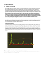
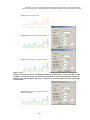
TABLE OF CONTENTS
TABLE OF CONTENTS ..........................................................................................................................................................1
1
INTRODUCTION .............................................................................................................................................................2
1.1
2
USING PROFILER ...........................................................................................................................................................4
2.1
2.2
2.3
3
COPAS SYSTEM TEMPLATE (FILE NAMEXXX.CSV) ...................................................................................................11
FCS FORMAT FILE (FILE NAMEXXX.LMD)..................................................................................................................11
SUMMARY DATA FILE (FILE NAMEXXX.TXT) .............................................................................................................11
PROFILE READER COMPATIBLE FILE (FILE NAMEXXX.DAT).......................................................................................13
PROFILE READER........................................................................................................................................................14
5.1
5.2
6
SUMMARY ....................................................................................................................................................................6
CONFIGURING PROFILER SORTING (CRITERIA FOR PROFILES) USING PEAK HEIGHT AND WIDTH ....................................7
CONFIGURING SORTING CRITERIA BASED ON NUMBER OF PEAKS ..................................................................................8
DATA STORAGE............................................................................................................................................................11
4.1
4.2
4.3
4.4
5
ACTIVATE PROFILER.....................................................................................................................................................4
SET PROFILER CHANNELS .............................................................................................................................................4
SET SCALING DISPLAY OF PROFILES .............................................................................................................................5
SORTING WITH PROFILER .........................................................................................................................................6
3.1
3.2
3.3
4
PROFILER: AN OVERVIEW ............................................................................................................................................2
PROFILE READER: AN OVERVIEW...............................................................................................................................14
THE DISPLAY OF A PROFILE........................................................................................................................................14
OPERATING PROFILE READER...............................................................................................................................15
6.1
OPENING A FILE ..........................................................................................................................................................15
6.2
SETUP THE PROFILE DISPLAY .....................................................................................................................................15
6.2.2
SCALE................................................................................................................................................................15
6.2.3
CHANNELS .......................................................................................................................................................16
6.2.4
LABELS..............................................................................................................................................................16
7
PROFILE SETTINGS FOR SORT CRITERIA...........................................................................................................18
7.1
USING PEAK COUNT SETUP .........................................................................................................................................18
7.1.1
Operation of peak count.....................................................................................................................................18
7.2
USING COMPENSATION ...............................................................................................................................................21
7.2.1
An example for using compensation ..................................................................................................................22
8
OTHER FEATURES.......................................................................................................................................................23
8.1
8.2
8.3
8.4
RESET TO TEMPLATE...................................................................................................................................................23
IMPORT A TEMPLATE...................................................................................................................................................23
FILTER ........................................................................................................................................................................23
EXPORT AS TXT FILE..................................................................................................................................................24
1 Introduction
1.1
Profiler: An Overview
The standard COPAS system measures the value of extinction and fluorescence signals by integrating each signal over
the time that the threshold signal is above the threshold value. The result for each signal is a single value that has
obscured any details of the changing intensity of the signal while the signal is being integrated. Therefore, an object
containing a small intense fluorescent spot and another object with a low diffuse level of florescence throughout would
appear the same despite dramatically different spatial organization of the fluorescence signal.
Instead of making a single integrated measurement of a signal, the Profiler option digitizes the instantaneous
signal level. The result is a list of successive point measurements made while the object passes through the flow
cell. An object containing a small bright fluorescent spot will produce a fluorescence signal with a corresponding
narrow peak, and the Profiler will digitize the peak into a succession of numbers that directly trace the
fluorescence peak as it passed through the flow cell.
The computer can now perform tests that will detect the presence of different colored fluorescent peaks for the short time
they were present in the original signal, and note how much each individually rises above its own background level.
This ability to detect short-duration signal peaks that would be swamped out by a single integrated measurement is one
way in which the Profiler can enhance detection sensitivity.
Positional information
An additional advantage of the Profiler is that all digitized points have been recorded proximally, along with the peak
signal, so that the position of the peak can be located proportionally in the total list of points. This permits extracting
positional information from the complete profile, rather than simply the presence or absence of peaks. Notice how the
fluorescence profile signal aligns with the microphotograph in Figure 1. Profiles can be collected for the changes in
optical density (which we refer to as extinction or EXT) and three fluorescence channels, along the length of the object,
simultaneously. This correspondence permits testing for the relative positions of fluorescent markers within an object,
allowing another dimension for resolving differences between the analyzed individuals in a collection or population of
objects.
70000
60000
50000
40000
30000
20000
10 0 0 0
0
Figure 1: C. elegans worm with str-1::GFP; mab-5::dsRed; unc-17::zsYellow
Profile of transgenic nematode clearly shows green expression in head, yellow expression in the animal’s vulva and red
expression in multiple specific cells along the body.
2
Variable scan rates for resolution control.
Additionally, Profiler gives the user the option of setting the scan rate (the clock rate of data storage) of the object itself as it
passes through the flow cell. There are six scanning rates available to the user ranging from 156 KHz to 5 MHz. A scan rate
of 156 Hz takes single integral measurements every 6.4 microseconds while at a rate of 5 MHz single integral measurements
are collected every 0.2 microseconds. This has an obvious effect on the resolution of the profile itself. Because higher scan
rates take integral parameter information slices more frequently than slower scan rates the result is better detection of slight
differences along the length of the object. Using higher scan rates, the profile of the object is one of sharper peaks and
valleys accurately depicting the small variations along the length of the object. Lower scan rates will in essence average the
highs and lows of variance to have an overall smoothing affect on the profile.
NOTE: For many users, the definition of multiple single peaks is advantageous in distinguishing minute
variations in the sample. However, it is important to note that higher scan rates require more computer
processing and can result in very large data files. It is important to consider testing different scan rates before
conducting a profiler experiment. More is not always better.
Multiple parameter data acquisition
Profiler allows for sorting based on profile features of multiple parameters as a secondary sorting mechanism for objects
fulfilling sort regions in dot plot. In the absence of profiler, most settings can be manipulated so that slightly differing
subpopulations are separated on the gate and sort dot plots. However, with activation of profiler, “sortable” objects fulfilling
dot plot criteria can be further analyzed for presence/absence of a peak of interest in one or more profiled parameters. This
means that a sort decision can be made based on any user defined profile features contained in one or more of the profiled
parameters. Moreover, specific sorting rules can be established for each profiled parameter independently, and only events
that fulfill ALL the sorting criteria will be dispensed.
Number of peaks
Finally, software can count one parameter’s peaks over the entire length of the object. Using user defined criteria, the system
will determine peaks within an object then compare to count limits set by user before a sorting decision is made.
3
2
Using Profiler
2.1
Activate Profiler
After normal startup of the COPAS instrument and COPAS software, activate the Profiler by checking the Profiler check
box on the screen. The area in the upper right hand corner displaying the sorting limits for TOF, EXT, and three
fluorescence colors will change to the Profiler display.
Figure 2: Screen capture of COPAS software main screen
The message READY should appear on the display in the lower area.
.
2.2
Set Profiler Channels
Using profiler will allow you to view profiles in real time for any combination of the parameters profiled. User can
choose any or all of the four parameter’s available Extinction, Green, Yellow, and Red fluorescence.
1.
Choose Profiling Parameters under the PROFILER pull down menu. A dialogue box will appear that allows you to
activate any combination of parameters to be displayed in the profiler window by checking the box next to each
parameter title.
2. At this time you can choose to change the color of a parameter’s display by clicking the “Change Color” button next
to the parameter you wish to modify.
3. Select one parameter to display its peak features during acquisition mode.
4. Implement the changes by clicking OK. The profile window will display the values of the chosen parameter
channel’s HIGHEST peak height and peak width (width above level defined in criteria for profiles) at the right side
of the profile window.
NOTE: The peak width determination is made based on user input in the “criteria for profiling” function.
See section 3.2 criteria for profiling.
4
2.3
Set Scaling Display of Profiles
The profile of each object will be displayed in the profile window so that a line graph of each parameter profiled
(correspondingly colored) will be graphed along the TOF measurement (x-axis). Because each parameter’s information will
be unique to each sample, it is necessary to set the display scale of each parameter independently. This allows the user to
adjust how each parameter is displayed in the profile window as the data is acquired.
1.
2.
3.
Open the Scale dialogue box under the PROFILER pull down menu. Two dialogue box tabs will be visible: profile
scaling, and dot plot scaling. Dot plot scaling serves as a summary of scales set for each parameter for their display
in dot plot mode.
Choose profile scaling tab to adjust the scaling of profiled parameter display.
Identify the X-axis scaling at the bottom half of the dialogue box. Use up or down arrows to select the maximum
TOF to set profile window display.
If you are using TOF on either the Gate or Sort dot plot displays it is best to set a maximum equivalent to the TOF in dot
plot scale. If profiler plots an object with a TOF larger than the maximum, the profile may appear truncated within the
profile window.
4.
5.
Identify the y-axis scaling. Set scaling for each profiled parameter by using up or down arrows at the right end of
the window. Keep in mind if a profiled parameter exceeds the limits set in scaling, the profile graph will contain a
flattened peak at the maximum y-axis value (upper scale limit). It may be necessary to change the scaling.
However, if you find that a peak exceeds system maximum value of 65536 (signal is saturating the channel’s storage
limits) you may consider changing scan rates, PMT, or gain settings for this parameter. See sections 7 and 9 in
COPAS manual for more information on changing these variables.
Select OK to implement scale settings.
NOTE: Scaling only affects how the profile is displayed, not the raw data generated. Scaling can be changed
at any time during data acquisition.
5
3
3.1
Sorting With Profiler
Summary
A sorting decision for every object passing through the flow cell consists of evaluating three different sets of
conditions:
a) HISTOGRAM MARKERS OR GATE AND SORT REGIONS.
Just as with the standard COPAS system, an object must lie inside any histogram markers or gate and sort
polygonal regions if it is to be dispensed. Non-profiling systems can have up to 5 parameters that can be used
as parameters for histogram markers or gating and sorting dot plots – TOF, EXT and three colors of
fluorescence. The Profiler provides additional parameters – Peak Height and Peak Width for EXT, and each
of the three fluorescence colors (green, yellow, and red). Any combination of these thirteen parameters can
be selected for dot plot displays. See section 7.12 Sort criteria in COPAS manual for more information about
sorting based on dot plot.
NOTE: The ‘Selected %’ at the top of the screen takes into account only the non-Profiler constraints
defined by dot plots, and is not affected by the Profiler constraints. Specifically, the following Profilerspecific conditions do not affect this number.
b) PEAK HEIGHT AND PEAK WIDTH LIMITS.
This set of sorting conditions is available only on Profiler systems. By setting limits for these two parameters
and selecting INCLUDE or EXCLUDE, additional constraints for an object’s being dispensed are specified.
If the user keeps these limits wide-open and/or selects the ACCEPT ALL option, then these parameters do
not participate in the sorting decision.
NOTE: if these Profile parameters are selected for dot plots, the conditions for the dot plots (polygons) and
conditions set in the profile configuration will be evaluated independently. For an object to be dispensed,
both sets of conditions must be satisfied simultaneously.
c)
PEAK COUNT (see configuring sorting based on peak count)
The user must specify a profiler channel under which to count peaks. The user can specify the desirable
number of peaks within the segment of a profile defined by ‘Location’ limits. Setting the range to the default
values of 0 and 250 removes the Number of Peaks from the sorting decision.
NOTE: Sorting based on peak count is a valuable sorting tool; employ; however, it requires very rigid
conditional limits to be useful. To configure peak counting successfully, the anticipated shape of a profile
should be understood. It is advisable to use ProfReader software on a test sample to optimize settings for
peak count implementation. See section 7.1 using peak count setup function in ProfReader software.
All the above conditions are evaluated independently and must be satisfied simultaneously for an object to be
dispensed. Any or all of these conditions can be configured so that they will be disregarded by setting limits to a
maximally wide range.
6
3.2
Configuring Profiler sorting (criteria for profiles) using peak height and width
1.
2.
3.
Open the criteria for profiles feature under the PROFILER pull down menu. The criteria for profiles dialog box
(shown above) will appear allowing the user to enter sorting limits (rules) for each profiled parameter.
Choose a parameter to set limits from the tabs at the top left corner of dialogue box.
Set limits for peak Max Height and peak Width above level by typing in values in the appropriate windows or use up
and down arrows at the right side of each window. See discussion on determining profiler criteria and ranges for
Peak Height and Peak Width determination.
Profiler Criteria and Ranges for Peak Height and Peak Width determination.
+
PEAK HEIGHT:
The highest measured value along the length of the object. Peak height measurement is compared with lower and
upper limits specified by the user. The limits can be set between 1 and 65536. Keep in mind that peak width sort
criteria depend on peak height low limit as value to determine peak width.
7
PEAK WIDTH:
The program identifies all areas of the profile that exceed the value of the lower peak height limit. The system
determines a width for every area of the profile contained above this value. See the figure above. The sum of all
width measurements is the peak width value. It is compared with lower and upper limits specified by the user. The
limits can be set between 0 and 4096.
4.
Choose to accept all, include, or exclude limits you’ve set when sorting the sample by choosing the appropriate
setting from the pull down tabs next to peak height and width range settings.
ACCEPT ALL
Ignoring the specified ranges for the ‘Peak Height’ and ‘Peak Width’, every object passing the flow cell will be
dispensed to a microtiter plate or sorted to a receptacle.
INCLUDE
Only those objects that are within the specified ranges for the ‘Peak Height’ AND ‘Peak Width’ will be dispensed to
a microtiter plate or sorted to a receptacle. The conditions for both parameters must be satisfied simultaneously.
EXCLUDE
Only those objects that are outside the specified ranges for the ‘Peak Height’ OR ‘Peak Width’ will be dispensed to
a microtiter plate or sorted to a receptacle. Either parameter falling outside its range will satisfy the EXCLUDE
condition.
NOTE: Remember objects can only be sorted if they have also met gate and sort region criteria as displayed
in dot plots.
5.
3.3
Set rules for sorting based on number of peaks by entering limits into the appropriate fields or using up and down
arrows next to each field. See discussion of setting appropriate limits for sorting based on peak count below. Or set
number of peak to ACCEPT ALL and location requirement to EVERYTHING which effectively removes peak
count from sorting decision and skip ahead to step 10.
Configuring Sorting criteria based on number of peaks
Before making a sorting decision, the software calculates the number of peaks in the acquired profile or part of a
profile based on user defined peak count criteria found in Peaks count setup under the PROFILER pull down menu.
After the entire Profile is scanned, the total number of peaks within defined location is compared to the limits set by
user.
6.
Click “Change peak count setup” button located beneath the location settings to open dialogue box (shown below) to
setup peak count. Set appropriate settings for determining peaks. See using profile reader section 7.1 using peak
count setup to optimize these settings.
VERY IMPORTANT: It is crucial to carefully setup peak count criteria accurately. Therefore
it is recommended that the user collects a number of representative profiles which (s)he can
8
manipulate in ProfReader software to determine acceptable settings for peak count setup prior
to sorting objects using number of peaks.
Under number of peaks, enter the range of numbers of peaks you wish to sort. Acceptable range is 0-250 peaks.
7.
Select sorting to Accept all, include, or exclude objects based on number of peaks.
ACCEPT ALL
Ignoring the specified ranges for the number of peaks, every object passing the flow cell will be dispensed
to a microtiter plate or sorted to a receptacle. This may be useful if user wants to count peaks as data is
acquired but doesn’t need to sort based on peak count number.
INCLUDE
To be dispensed to a microtiter plate or sorted to a receptacle an object must satisfy the following condition:
The profile has a number of peaks satisfying the “Number of Peaks” limits and these peaks are within the
predefined “Location” limits along the length of the profile.
EXCLUDE
This condition is the compliment of INCLUDE. In other words, only objects not satisfying the condition for
INCLUDE will be dispensed to a microtiter plate or sorted to a receptacle. If a sample usually exhibits 1 to 2
peaks of localized fluorescence, it may be possible to sort variable expression patterns by EXCLUDING objects
with 1-2 peaks. By doing this the user can collect objects with no fluorescence or objects with more than the
usual two peaks of fluorescence.
8.
Set peak location ranges by entering an appropriate range of the entire length of the object to count peaks in.
Location of peaks is the relative position of peaks, expressed as a % of length of the whole object, in a profile
that can be chosen. This allows the user to specify a segment over which the number of peaks is evaluated.
Notice that user MUST set limits to EVERYTHING, MIDDLE, or ENDS to evaluate peaks over any length of the
object.
EVERYTHING ignores limits set.
Peaks along the whole profile are included in the ‘Number of Peaks’ count; the ‘Location’ limits are
disregarded.
MIDDLE will check for peaks appearing within the % limits set.
Only peaks between the ‘From’ and ‘To’ ‘Location’ limits are included in the ‘Number of Peaks’ count.
ENDS will check for peaks satisfying criteria outside the % limits set by user.
Only peaks outside the ‘Location’ limits are included in the ‘Number of Peaks’ count, i.e. only the ‘heads’ and
‘tails’ outside the middle are taken into account.
9.
Set sorting rules by unchecking the “do not set sorting rules for this channel” located at the top left corner of
dialogue box. Summary on right half of dialogue box should reflect the rules you have implemented.
NOTE: Unchecking the “do not set sorting rules for this channel” automatically activates the system to
check ALL profiling criteria peak height/ width AND number of peaks. Be sure to set appropriate limits
for all profiling parameters or wide enough limits that allow the system to ignore peak height/width or peak
count analysis if necessary.
10. Click APPLY button at the bottom of the dialogue box to implement all the rules you have set.
-9-
11. If desired, select other parameter channels to apply sorting rules for peak height and peak width.
NOTE: User can apply profiler rules for peak height, peak width and number of peaks to none, one, or any
combination of parameters profiled. Keep in mind that if many profiling rules apply there may be no
events that will pass all of them.
12. Click CLOSE to close the dialogue box and return to COPAS program screen.
13. Once settings have been chosen, initiate a sort manually or fill plate making sure that you use Data Collection
mode to acquire the sample. See section 4 sorting in COPAS user’s manual.
14. You can store your data after acquisition.
- 10 -
Data Storage
4
Once data is acquired, data can be stored by clicking the STORE button at the right edge of the COPAS software screen.
When data is stored, four files are created that correspond to the data storage event.
4.1
COPAS System template (file nameXXX.csv)
The csv file contains settings for the COPAS system preserved at the time of data acquisition. All settings such as PMT,
gains and gate and sort regions are stored as a template that the user can open later if they wish to run additional samples
under previous conditions.
NOTE: Sample may not fall within previous gate and sort regions for various reasons. 1. Slight differences
in sample conditions may result in minute physical changes that the instrument can detect. Starvation for
example, may cause changes in the object’s internal structures, the EXT (optical density) measurement may
reflect this difference. 2. System pressure changes between samples may cause similar objects to be analyzed
differently. For example, if sheath pressure is set too high (resulting in a faster sheath flow rate), objects
carried in that flow will move past the laser faster than under normal flow rates resulting in a smaller TOF
measurement. Comparing samples acquired under different sheath pressure conditions may look slightly
different for this reason.
4.2
FCS format file (file nameXXX.lmd)
This format is compatible with most flow cytometry software such as FCSExpress. The file contains all measured integral
parameters (extinction, fluorescence) , TOF and peaks’ parameters (height and width) for every channel. . See COPAS
system manual section 7.10 data storage.
4.3
Summary data file (file nameXXX.txt)
Summary data file contains all data points stored after data acquisition. Data is organized into columns as described next.
DESCRIPTION OF COLUMNS IN THE SUMMARY DATA FILE (also described in the COPAS system manual)
ID
Sampled objects are given a chronological identifying number starting with 0. This identifier is preserved in
txt and DAT files (profiler reader) so the same object event can be identified in both files.
PLATE
Plates are indexed in chronological order when dispensing into or aspirating from a microtiter plate using a
Plate Handler (Twister). If dispensing into or aspirating from a plate without a Plate Handler, this
column will always contain ‘1’.
If dispensing in a receptacle (Manual Sort) or scanning without dispensing, this column will contain ‘-1’.
ROW
If dispensing into a plate – a well’s (numerical) row index (A, B, etc), as seen on the plate’s template. It is
necessary to align the plate correctly to utilize this.
0- display if not using plate format.
COL
If dispensing into a plate – a well’s (alphabetical) column index (1, 2, etc), as seen on the plate’s template. It
is necessary to align the plate correctly to utilize this.
0- display if not using plate format.
CLOG
If software detects a clog while sampling file will contain a Y otherwise an N will be displayed to indicate no
problem during sampling.
- 11 -
SCAN RATE
A single scan rate must be used to generate profile data. This rate is displayed as:
156=156 KHz, 312=312 KHz, 625=625 KHz, 1250= 1.25 MHz, 2500=2.5 MHz, 5000=5 MHz
STATUS SORT
A number representing the sorting status of an event, returned by COPAS board.
Refer to the following key:
0- scanning without dispensing
1- unknown, sort status cannot be retrieved
2- out of region
3- in enhanced mode: coincidence with following, un-sortable, event
4- coincidence in pure mode
5- lost synchronization during acquisition, not sorted
6- sorted
7- sorted in superdrop
8- in enhanced mode: coincidence with previous, un-sortable event
9- sorting decision took too long for event to be dispensed
3n- Sort status equal 30+n, where n is one of the above statuses, indicates that the object was very close
to the previous object, and the sorting drop (if n = 6) started at least 30 microseconds later than it
normally should have.
STATUS SELECT
A Selected status is assigned to each object with respect to its parameter’s relative to the gate and sort regions
and with respect to its profiler characteristics relative to the chosen Profiler sorting configuration.
0- outside TOF (histogram) gate
1- outside gating 2-dimensional region (dot plot)
2- outside sorting 2-dimensional region (if sorting based on 2d regions) or does not satisfy any
histogram condition (if sorting based on histograms)
3—10- does not satisfy a condition for peak’s height or width
40– satisfies all sorting conditions
NOTE: Display/Store options affect which data points are stored. Option EVERYTHING stores events
from every status select code (all data points). Option STORE GATED excludes events with status select 0
and 1 (outside gate regions). STORE SELECTED excludes events with status select 0, 1, and 2 (outside
gate and sort regions).
TOF
Time of flight value
EXT
Extinction integral value
Green, Yellow, Red
Integral values for fluorescence on a corresponding channel.
PH Ext, PH Green, PH Yellow, PH Red
Maximum Peak Height of an individual profile.
In non-Profiler configuration – ‘0’
PW Ext, PW Green, PW Yellow, PW Red
Peak Width of an individual profile (SEE DEFINITION ENTER REFERENCE).
In non-profiler configuration – ‘0’.
PC Ext, PC Green, PC Yellow, PC Red
Number of peaks within selected location on an individual profile (ENTER REFERNCE LKOCATION).
Otherwise displays n/a. In non-profiler configuration – ‘0’.
- 12 -
At the bottom left corner of the txt file is a summary of the conditions under which the sample was run. These
include the displays of:
Threshold source
This is the trigger on channel and displays the value of this threshold setting.
Min TOF = #,
TOF threshold value
Signal gains for EXT, GREEN, YELLOW, and RED color channels
PMT voltage of each color channel
Data string indicating the location and name of the CSV file corresponding to this data acquisition.
4.4
Profile Reader compatible file (file nameXXX.dat)
The DAT file is a unique system file only compatible with ProfReader software included in the Profiler package. This file
allows profile specific portions of the txt file to be displayed for visual analysis. Object profiles displayed will appear as
they did in the profiler window during data acquisition.
- 13 -
5
Profile reader
5.1
Profile Reader: An Overview
Profile reader is a feature provided with the new profiler II package that converts the stored DAT file to composite
line graphs displaying the profiled parameters for a single analyzed object. Profile reader can be used simply to display
stored profiles or as a tool to optimize settings for viewing and/or sorting based on the unique characteristics of a particular
sample in profiler mode. The following contains information for an in-depth look at how to use profile reader.
Figure 1. Screen print of profiles viewed through profile reader. Notice the display features of the profiles include
overlaying graphs of each profiled parameter (green, yellow, and red). In this case EXT was not profiled. Highest
peak and width above level are displayed for each parameter as well as the scale value for TOF
5.2
The Display of a Profile.
Profiles are plotted with the time of flight of the object along the x-axis. The value at bottom right of the screen
displays the TOF at that point. The y-axis contains successive profile channels that contain integral signal data for each
parameter profiled. The display can be thought of as overlaying line graphs of each parameter (correspondingly colored)
plotted along the object’s length. Specific to each profile, are the parameter displays demonstrated at the top of the screen.
Profile index
NEXT/PREVIOUS
SHOW
Highest peak
Width above level
COUNT PEAKS
This is the profile identifying number that corresponds to its location in the txt file of the stored
data.
These activity buttons allow the user to scroll through successive profiles ordered by index
number.
This activity button that allows the user to advance to that specific profile when user inputs the
number in the index window then clicks this button.
This is a numerical value of the parameter’s highest peak within the currently displayed profile.
This is the summation of all peaks’ widths as determined at the user defined “calculate width on
level” (under channels feature) for the currently displayed profile.
This activity button opens up peak count dialogue box.
- 14 -
6
Operating Profile Reader
6.1
Opening a File
Select “Open” under the FILE drop down menu and find the appropriate DAT file to open.
Upon opening a DAT file in Profiler reader, the software automatically searches for a matching CSV file for use as a
template. When a matching template is found, the profile reader is automatically initialized with the profile criteria settings
used during data acquisition. This gives the user immediate display of profiles as they appeared during data acquisition as
well as the settings used for COPAS display and/or sorting of the sample.
If a matching template is not found a message appears stating this. When this happens, user must click OK button on
the message before the file will be opened using default settings. At this point, the user can choose to import a template (see
Import Template, section 4.4) or set up the program for visual analysis of the profiles using SETUP menu features.
6.2
Setup the Profile Display
6.2.2 SCALE
“Scale” lets the user choose the scale in which each parameter is independently displayed.
1.
Open the scale feature from the set up pull down menu. (Dialogue box shown above)
2.
Scale the X axis (Time of Flight) by entering an integer, selecting adjustable range, or range based on scan rate.
If a value is entered only the left channels up to that number will be displayed in the viewer window for every
profile in that DAT file. If profiles are longer than the scale range set, only the left part of the object contained
within the viewer limits will be displayed.
If the user chooses to select adjustable, each profile will be scaled to fit within the window.
NOTE: Choosing adjustable scale will make it very useful to scan through profiles of objects with varying
lengths within a DAT file. However, it can also make these profiles harder to compare to each other. Peak
widths, for example, may appear very different between objects of various lengths.
Choosing “Scale X axis to instrument units” causes converting profile’s total length and peak’s width to the
TOF units, i.e. 0.4uS. Correct scan rate is essential for the conversion. If this option is not checked then all values
along axis X are presented as number of scanned points. It is important to use this option if you use ProfReader to
configure peak counting or sorting criteria. The template will automatically fill in scan rate when file is opened.
Scan rate can be found listed in the original TXT file should the user want to use this option in the absence of having
a viable template.
3.
Scale the Y-axis parameters by entering integers or selecting adjustable setting for each parameter.
The scale range can be any integer from 1 (flat line on the x axis) to 65536 (the highest signal level detectable
by the filter). Again, each profiled parameter is independently scaled allowing you to see different parameter
features of the profiles. Selecting “adjustable” will change the scale so that the parameter range of the profile fills
the entire viewer along the y-axis.
4.
Click OK to implement scale setup and return to viewer display window.
6.2.3 CHANNELS
“Channels” allows the user to choose which parameter channels to display in the viewer and where to set the level
of width determination.
1.
Open the dialogue box by selecting CHANNELS from the SETUP pull down menu. (See dialogue box above)
2.
Click on the profiled parameters you want displayed in the viewer. A check mark in the window indicates the
parameter will be displayed. A “ghosted” parameter indicates that the parameter channel was not selected for data
storage during data acquisition.
3.
Choose a value to calculate width on by typing in an integer or clicking the up or down arrows next to the
appropriate window. Appropriate range is integer 1 to 65536 (maximum y value).
The calculate width on level is used to determine where the width of a peak is calculated. This can be
particularly useful for two reasons: 1) to help determine length of the object that rises above the calculate width on
that specific level, 2) visualizing where an absolute peak height value lies on the graph. For instance, if EXT was
used as the trigger channel, the user can determine the TOF by entering 1 as the EXT calculate width on level.
Under these conditions, the entire profile will be contained (begin and end) within the peak of EXT of at least 1.
Therefore, the width above level for EXT signal displayed at the top of each profile will equal the object’s TOF.
Additionally, drawing a height value on the graph is useful in the peak count mode described in using peak count,
section 7.1.
4.
Click Apply to implement the changes.
5.
Click OK to return to the viewer window. Upon returning to the viewer window, you should see that peak width
calculations have changed and that a horizontal line was drawn across the graph at the calculate width on level for
each parameter profiled.
6.2.4 LABELS
"Labels" allows the user to change the title and color display of a profiled parameter channel.
1.
Open the LABELS dialogue box under the SETUP pull down menu. (See dialogue box above)
- 16 -
2.
3.
4.
5.
6.
Choose a parameter channel to modify.
Change the title by typing in the new title under the corresponding Label window.
Change the color of the display by clicking on the Channel’s Change color button.
Select a color you wish it changed to, clicking OK when done to close the color change dialogue box.
When all changes have been made to Channels, click OK to implement the changes. The profile viewer will reflect
the title and color changes.
- 17 -
7
7.1
Profile Settings for Sort Criteria
Using Peak count setup
Peak count identifies and counts peaks on any one profiled parameter channel based on user-defined criteria. The
criteria can then be used in COPAS software to make peak count sorting decision.
When activated, the COPAS profiler uses peak count as final criteria for sorting a sampled object. The ProfReader
software serves as a tool to determine appropriate settings, specific to individual samples, for using this sorting feature of
the software. Peak count is a feature that as the name suggests, counts the number of peaks that fulfill user-defined
criteria. See above figure of the dialogue box
7.1.1 OPERATION OF PEAK COUNT.
1.
2.
3.
Open the Peak Count Setup feature by selecting it from the SETUP pull down menu. (See the dialogue
box above)
Choose a profiled parameter to count peaks over. Do this by locating the channel window and pull
down menu towards the top of the box; options available are any of the parameters profiled during data
acquisition such as Ext, green, yellow, or red fluorescence.
Choose the number of data points to average the graph over by using up and down arrows next to the
‘average on’ feature tool. See the discussion below to determine a value to average on.
Average on value
The program looks at every data point of the profile, averaging data values from surrounding
channels to construct a smoothed graph to determine peaks over. For example, if the user selects 5
channels to average on, the value displayed in channel 12 will be the average value of data from
channels 10-15. This is designed to remove the little variations in fluorescence along the profile in
essence reducing the fluctuations based on noise.
Consider the scan rate.
Higher scan rates generate a data point as often as every 0.2 microseconds. The data reflects a
very small slice of the total length of the object. Conversely, the slowest scan rate collects data over
6.4 microseconds as the object passes the laser path. Effectively, each data point contains
information over a longer slice of the total length of the object. One way to think about this is to
consider that each data channel generated using the slowest scan rate may contain information that
spans up to 32 channels generated using the highest scan rate. Therefore, averaging on 5 channels of
156 KHz scan rate is akin to averaging 160 channels under 5MHz scan rate. The averaging effect
can be quite large so keep this in mind when choosing a value to average on.
Once the user inputs the number of channels to average on, the “smoothed” profile is drawn in black on
top of the actual profile and this becomes the profile line graph that the program uses to determine and
count peaks.
- 18 -
4.
Determine a threshold value for determining a peak. This is the peak’s absolute height greater than
value in the peak count dialogue box. See the discussion of peak’s absolute height below. Enter an
integer into the window.
Peak’s absolute height greater than
The absolute height of the peak is a signal level that the graph needs to rise above in order to
be analyzed as containing peaks. Keep in mind that any area of the profile that does not meet this
value will be excluded from analysis as a peak, so it is important to determine a height sufficient
to contain all peaks of interest. For this purpose, it is useful to set the calculate width on value
found in channels menu equal to your absolute height value?????why not maximum or
minimum?. By doing this, the “absolute height value will be drawn across the graph, offering
visual display of which peaks rise above this height.
Choosing different values will allow you to see which peaks are above (considered for peak
count analysis) and which peaks on the graph are below the absolute height (will totally be
excluded from analysis). See figure below that shows how different absolute height values affect
the peaks counted. Note that changing the value of absolute peak height changes the number of
peaks counted.
Figure 2A: absolute height = 500, number of peaks = 28
Figure 2B: absolute height = 2000, number of peaks = 18
5.
Choose a value for “Peak’s relative height greater than” by inputting a value lower than the “Peak’s
absolute height greater than” value. Peak’s relative height greater than will determine where each
“potential” peak’s width is calculated. See discussion below to determine peak’s relative height greater
than.
Peak’s relative height greater than
Once the program identifies an area of the profile that meets peak absolute height, it locates
each individual peak maximum value and analyzes these points for peak relative height and peak
width. At each maximum, the program moves down the peak the distance of the user-defined
relative height to determine the width of the peak at this point. Basically, the program extends a line
across the peak at this height (peak height – relative height). Wherever the line intersects with the
graph twice it creates endpoints that it will measure to determine the width of this peak. This
distance is the single peak’s width.
- 19 -
The value set for relative peak height affects which peaks are counted. See the figure B and C
below where an increase of 100 in the relative peak height excludes four peaks from peaks counted.
Figure 3A: part of original profile
Figure 3B: relative height = 200, peaks counted = 11
Figure 3C: relative height = 300, peaks counted = 7
NOTE: Keep in mind that neighboring peaks may interfere with each other if limits are too large. For
example, it is possible that a series of neighboring small peaks will be labeled as a single peak with a width
extending over all of them. In this case the tallest peak is labeled as a peak and the program will draw the
width over the graph of multiple small peaks as in figure D. To avoid this, tighten the relative peak height
and width limits.
Figure 3D: relative height = 700, peaks counted = 6,
width range changed.
- 20 -
6.
Set limits for single peak’s width. Set upper and lower limits for the peak width for peak analysis by
entering values in the “Single peak’s width from” boxes. Determined width of peak must lie within
these limits to be counted as a peak.
NOTE: a generous set of limits will favor counting many peaks while a smaller range may exclude peak
widths just outside either end of the limits. It is useful to determine the best set of limits by applying different
value sets to see which works best for your sample.
7.
8.
9.
Click Apply to implement all the settings.
Click OK to close the dialogue box and return to viewer screen. Profile viewer will have additional items
displayed. A black line (average on) graph closely laid over the parameter channel used to count peaks
should appear on the display. Additionally, user should see individual peaks labeled with a p and light
blue lines across each peak denoting where the width measurement was made. At the bottom left corner
there will appear a new data display: peaks counted = the number of peaks (labeled with p) that fulfill
peak count criteria.
Using NEXT and PREVIOUS buttons, scroll across other profiles in the same DAT file to ensure settings
are sufficient for other object profiles. It is possible you will need to adjust some of the settings a few
times to correctly count important peaks from different objects.
At this point, the values determined for correct peak analysis and count can be input into the COPAS software
program and sorting can be performed using new peak count criteria. See software peak count feature for more
information about this.
7.2
Using Compensation
“Compensation” allows the user to manipulate the display of fluorescence overlap by removing a percentage of one
color emission from the emission of another fluorochrome.
Figure 6. Emission spectra: green line: green emission, blue line:
yellow emission, red/orange line: red emission.
green block: green detector bandpass filter, yellow block: yellow
detector bandpass filter, red block: red detector bandpass filter.
The COPAS instrument uses either of the two excitation filters (488nm and 514 nm) to get the different
fluorochromes emissions that are absorbed by the PMT’s. Despite the fact that bandpass filters are used to best capture
individual color fluorescence, there is still a considerable amount of fluorescence overlap between the color parameters.
The figure above shows the color spectrum overlap of the color channels the instrument uses. Clearly there is a broad
area of overlap of the emission spectra of the three colors detected, especially in emission of green and yellow
fluorescence. The result is that parameter signals often contain some portion of another color’s emitted light. For the
purposes of displaying an object’s fluorescent characteristics, it may be necessary to adjust for this emission overlap.
1.
Open the compensation dialogue box from the SET UP pull down menu. The dialogue box lists each
color parameter as an independent function and the remaining two colors as a variable amount for
compensation.
- 21 -
2.
Choose a parameter channel to be modified. If subtracting green emission from yellow detector, choose
the yellow signal bar and move K1 cursor (green signal) right to desired percentage to be subtracted.
This percentage value appears in the box to the right of the sliding bar.
3.
Click APPLY then OK. The profile display will change to reflect the compensated values.
7.2.1 AN EXAMPLE FOR USING COMPENSATION
To better understand fluorescence compensation, it is useful to look at a profile where this is occurring. Shown
below is part of a profile where the “green and yellow scale settings” are set equal to each other. You’ll notice that
there are two yellow peaks about midway along the graph. The green graph at this place does not show peaks.
However, at the right end of the profile there is a large peak displayed for both the green and yellow parameters but
phenotypically there should be only one color fluorescence (green) at this point. It is quite likely that the
overlapping peaks in both parameter channels is due to overlap of spectra and absorption of green signal by the
yellow detector. Compensating for green by removing 50% of the green signal from the yellow signal, we can
clearly see the difference between graphs of the same object. Notice that the yellow peaks at the middle of the
object have not been altered much by removing a portion of the green signal from the yellow data. However, the
peak at the far right is greatly reduced. This suggests that the yellow peak at that end of the object is comprised
mostly of green signal. This may be very useful knowledge in determining how to conduct your sampling keeping
two things in mind: 1) all compensation values used in ProfReader software can be duplicated in the COPAS
software for determination of compensated parameter values, 2) conducting compensation function during profiling
is time consuming and may result in too much processing time for accurate sort decision.
Note: compensation should be set using dual parameter Dot Plots in the acquisition software and using
approprioate controls for correct values.
Figure 7A. Original profile
Figure 7B. Compensated profile: yellow signal reduced by
50% green signal. Note: reduced yellow peak
- 22 -
8
Other Features
8.1
Reset to template
The “Reset to template” feature allows the user to revert any changes back to original template settings. Only
pertains to a file where original matching template was found. To do this simply click on the Revert to template under SET
UP pull down menu and all modified values will be reverted to values contained within original template. If a template was
not found, the viewer cannot revert to a template and all settings simply maintain the values currently in use.
8.2
Import a template.
It is possible to open a DAT file and import template scale settings used during a different sample’s acquisition.
1.
2.
3.
8.3
Select import a template in the FILE pull down menu.
Select the CSV file from the template you wish to use.
Select OK. Imported template settings will temporarily replace the existing ones. Template settings will only be in
effect until the file is closed. If file is opened again later, data will be displayed using original settings from data
acquisition.
Filter
“Filter” allows the user to set criteria so that only significant object profiles contained within the larger stored data
are displayed while scrolling through the individual profiles.
Choosing this feature opens the criteria for profiles dialogue box from the COPAS software. See Profiler manual
profiling sort criteria for a detailed description on how to set criteria for profiles to be used as a filter. Here the user can
select any parameter in which to use as a filter simply by setting limits and applying the set criteria for this parameter box.
This can be particularly useful when the user needs to locate individual significant profiles from a file containing many other
profiled objects.
1.
2.
3.
4.
5.
6.
Open the filter feature under the SET UP pull down menu.
Choose a profile channel or multiple channels to set filter limits. (Extinction, Green, Yellow, or Red)
Set appropriate limits to include profiles with attributes you are interested in viewing or exclude profiles with
attributes you do not wish to view. For example, it is possible to “accept all” or “reject all” profiles with a peak
height above a user defined low-high range.
Choose to set rules for a parameter by unselecting the “Do not set sorting rules for this channel” found at the top left
of the dialogue box.
Click Apply to implement the limits you have set for a parameter channel. The right half of the dialogue box
(Summary) changes to reflect the sorting rules applied to this parameter channel.
Continue setting filter limits for other parameter channels, removing the “Do not set sorting rules for this channel”,
and Appling the limits set.
- 23 -
7.
Click CLOSE button to implement the filter criteria you have set. Once limits are set and applied, scrolling through
profiles by clicking "next" and "previous" will result in skipping over profiles that fail to meet the limits set by user.
NOTE: The specific limits set by the user are unique to individual samples. Therefore, the user should have a
good understanding of the characteristics in the profiles they wish displayed before setting filter limits. As an
additional note: once acceptable limits are established to VIEW profiles, these limits can be duplicated in the
Criteria for profiles box in the COPAS software to effectively display, sort and/or store object events fulfilling
these criteria limits. However, before applying these rules make sure you are very confident in your determined
settings. It is always advisable to test your settings with a small sample using an existing template (to ensure
consistent PMT, gain, threshold, scan rate settings, etc) before collecting large data acquisitions.
8.4
Export as TXT file.
The raw data from any single profiled object or series of objects can be exported as a txt file to be used for generating a
profile chart for statistical analysis.
1.
2.
3.
Select export as txt option from the FILE pull down menu. A dialogue box will be opened.
Choose a source file from which data will be exported (the default is set to the currently open DAT file).
If you check “Create separate file for each well” the software will use the summary text file to access wells
information and split data into separate files per well. By default the summary text file is in the same directory as the
.dat file and has the same name. This is the way how Copas software creates it. If it is located in different directory,
browse to it using Browse button at the bottom of the dialog.
4. Option “export data for different channels in separate files” means that – each exported file will contain data only
for one channel if you have acquired more profiling channels.
NOTE: if only one channel is collected for profiling, exporting different channels or selected channels only is
not meaningful.
5. Option “export data for selected channels only” allows exporting not all channels contained in .dat file. Only
channels selected in Setup/Channels (channels displayed on the graph) will be exported.
6. All options can be checked independently from one another.
7. Select a profile or group of profiles to export by entering the corresponding index number(s) you wish to export in
the “From” and “To” boxes as shown above left. The maximum number of events per file can be selected in the
same dialog.
NOTE: if a data file from a ReFlx acquisition contains more than 100 events per well you have to set this number
high enough to export all profiles from one well in the same file.
8. Click OK. At this point a new dialogue box will be opened shown above right.
9. In the File name window type in a name for the new file(s).
10. Click the Save button.
- 24 -
File names:
In general, exported files are named “name_channel_Px_Wy_z.txt”, where
name – name selected by user,
channel – name of a channel, e.g. green, red, etc., if exporting data separately per channel, otherwise omitted
x – number or name of a plate (from Plate column in summary file) if exporting data per well
y – well, e.g. A1, if exporting data per well
z- sequential numbers starting from 1 in case data should be split between several files.
NOTE: If you check the option “Create separate file for each well”, the selection of a group of profiles to export
(default 1 through 100) does not apply (note that it gets grayed out). With this option checked all profiles
contained in .dat file will be exported.
If you apply this option to the data collected not during sampling or dispensing, then the exported file(s) will look
as if all data belongs to one well (W00, because in the summary text file column and row are 0s, if only acquiring).
The txt file(s) generated will contain (depending the export finction) unlabeled data column(s) for profiled parameter(s):
EXT, green, yellow, and/or red. The data from export of multiple profiles will also be organized in columns and grouped by
object. The object’s index number can be found in the very last row of each data column.
At this point the user can select the data from the txt file and import it into whichever statistical or graphing software program
they wish to use.
- 25 -