Download STUK - Julkari

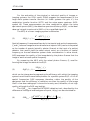
STUK-A196 / M AY 2003
OBJECTIVE MEASUREMENT OF IMAGE
QUALITY IN FLUOROSCOPIC X-RAY
EQUIPMENT: FLUOROQUALITY
M. Tapiovaara
STUK • SÄTEILYTURVAKESKUS
STRÅLSÄKERHETSCENTRALEN
RADIATION AND NUCLEAR SAFETY AUTHORITY
Osoite/Address • Laippatie 4, 00880 Helsinki
Postiosoite / Postal address • PL / P.O.Box 14, FIN-00881 Helsinki, FINLAND
Puh./Tel. +358 9 759 881 • Fax +358 9 759 88 500 • www.stuk.fi
The conclusions presented in the STUK report series are those of the
authors and do not necessarily represent the official position of STUK
ISBN 951-712- 688-3 (print)
ISBN 951-712- 689-1 (pdf)
ISSN 0781-1705
Dark Oy, Vantaa 2002
Sold by:
STUK – Radiation and Nuclear Safety Authority
P.O. Box 14, FIN-00881 Helsinki, Finland
Phone: +358 9 759 881
Fax: +358 9 7598 8500
STUK-A196
TAPIOVAARA Markku. STUK-A196. Objective Measurement of Image Quality
in Fluoroscopic X-ray Equipment: FluoroQuality. Helsinki 2003, 50 pp. + apps.
13 pp.
Keywords medical imaging, x-ray imaging, fluoroscopy, image quality,
statistical decision theory, ideal observer, quasi-ideal observer, detectability,
signal-to-noise ratio, SNR, accumulation rate of the signal-to-noise ratio
squared, SNR2rate, Wiener spectrum, spatio-temporal noise power spectrum,
NPS, temporal lag, optimisation, quality control, measurement method,
computer program
Abstract
The report describes FluoroQuality, a computer program that is developed in
STUK and used for measuring the image quality in medical fluoroscopic
equipment. The method is based on the statistical decision theory (SDT) and
the main measurement result is given in terms of the accumulation rate of the
signal-to-noise ratio squared (SNR2rate). In addition to this quantity several
other quantities are measured. These quantities include the SNR of single
image frames, the spatio-temporal noise power spectrum and the temporal lag.
The measurement method can be used, for example, for specifying the image
quality in fluoroscopic images, for optimising the image quality and dose rate in
fluoroscopy and for quality control of fluoroscopic equipment. The theory
behind the measurement method is reviewed and the measurement of the
various quantities is explained. An example of using the method for optimising
a specified fluoroscopic procedure is given. The User’s Manual of the program is
included as an appendix. The program is available free of charge for research
work and program evaluation purposes by contacting the author.
3
STUK-A196
TAPIOVAARA Markku. STUK-A196. Objective Measurement of Image Quality
in Fluoroscopic X-ray Equipment: FluoroQuality. Helsinki 2003, 50 s. + liitteet
13 s. Englanninkielinen.
Avainsanat
lääketieteellinen kuvantaminen, röntgenkuvantaminen,
läpivalaisu, kuvanlaatu, tilastollinen päätöksentekoteoria, ideaalinen
havaitsija, kvasi-ideaalinen havaitsija, havaittavuus, signaali-kohinasuhde,
SNR,
signaali-kohinasuhteen
neliön
kertymänopeus,
SNR2rate,
spatiotemporaalinen kohinan tehospektri, NPS, kuvan hitaus, optimointi,
laadunvarmistus, mittausmenetelmä, tietokoneohjelma
Tiivistelmä
Raportti kuvailee STUKissa kehitettyä FluoroQuality-nimistä tietokoneohjelmaa, jota voidaan käyttää lääketieteellisten läpivalaisulaitteiden kuvanlaadun mittaamiseen ja analysointiin. Mittausmenetelmä perustuu tilastolliseen päätöksentekoteoriaan ja keskeisin mittaustulos on signaali-kohinasuhteen neliön kertymänopeus (SNR2rate). Kuvadatasta analysoidaan myös
muita suureita, kuten yksittäisten videokuvien signaali-kohinasuhde (SNR),
spatiotemporaalinen kohinan tehospektri ja kuvan hitaus (lag). Mittausmenetelmää voidaan käyttää esimerkiksi läpivalaisukuvan laadun ilmaisemiseen, läpivalaisun kuvanlaadun ja potilaan annosnopeuden optimointiin sekä
läpivalaisulaitteiden laadunvarmistukseen. Raportissa on katsaus mittausten
taustalla olevaan teoriaan ja eri suureiden mittausmenetelmät on selostettu.
Esimerkkinä näytetään menetelmän käyttö erään läpivalaisututkimuksen
optimoinnissa. Ohjelman käyttöohje on raportin liitteenä. Ohjelman
käyttölisenssin saa tekijältä ilmaiseksi tutkimustarkoituksiin ja mittausmenetelmän käyttökelpoisuuden arviointiin.
4
STUK-A196
Contents
Abstract
Tiivistelmä
1
Introduction
2
Background
2.1 General concepts of image quality
2.2 Basic factors of image quality: MTF, contrast and NPS
2.3 Summary measures of image quality: SNR, NEQ and DQE
2.4 Visual assessment
3
The image quality quantities measured with FluoroQuality
3.1 Notation and conventions
3.2 Average images
3.3 The net signal and its frequency spectrum
3.4 The NPS of individual image frames
and the spatio-temporal NPS at zero temporal frequency
3.5 The full spatio-temporal NPS
3.6 The SNR-measures obtained by integration
(analytical biased data)
3.7 The SNR-measures obtained by integration
(analytical de-biased data)
3.8 Temporal lag
3.9 The DCsHFs-observer’s SNR obtained
using the template method
3.10 SNR2rate
3.11 Bias issues of SNR measurements
4
SNR2rate and detail visibility
5
An example of using FluoroQuality for
imaging technique optimisation
6
Acknowledgements
7
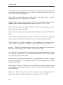
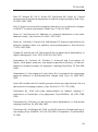
References and further reading
3
4
6
8
8
10
13
20
22
22
23
23
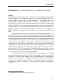
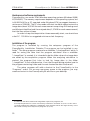
APPENDIX A: FluoroQuality (v. 2.0) User’s Guide
APPENDIX B: Interpretation of the data in xyzxyz.txt
APPENDIX C: Which files are necessary to keep
and the contents of the datafiles
APPENDIX D: The files and file formats required
from the acquisition program
51
58
24
25
25
26
28
28
30
30
36
39
45
46
59
61
5
STUK-A196
1
Introduction
This report describes FluoroQuality, a computer program that is intended for
the measurement of physical image quality in medical fluoroscopic equipment.
The measurement method of the program is based on statistical decision theory
(SDT), and fluoroscopic image quality is described primarily by the
accumulating rate of the square of the signal-to-noise ratio (SNR) of the ideal
(and a quasi-ideal) observer’s decision variable. These SNR2rate:s relate to the
detectability of a specified static detail in the image sequence by the ideal (or
quasi-ideal) observer. The measurement is made by adding and removing the
detail of interest in or from the phantom being imaged and analysing these
recorded image data. By choosing the phantom so as to sufficiently mimic the
scattering and attenuation of radiation in a patient, and choosing a detail that
mimics a diagnostically important detail in the x-ray examination, the
measurement should be closely related to the clinical quality of actual patient
imaging. By varying the phantom and the detail to be detected, various
detection tasks (see also Hanson 1983) can be considered, according to the x-ray
examinations of interest. In addition to SNR2rate the program produces also
other quality related data which should be useful in evaluating the
performance of the imaging system and for constancy testing.
The phantom need not necessarily be homogeneous – in principle, also an
anatomic phantom may be used. However, high-contrast phantom structures
may violate the assumption of noise stationarity and therefore make the noise
power spectrum measurements uncertain. Such phantom structures may also
make the detectability of the detail dependent on its specific location in the
phantom, and therefore achieving a good repeatability of SNR-results may be
difficult. Therefore, it is recommended to use a homogeneous phantom for most
measurement applications.
Unfortunately, because of the lack of a standard for recording image
data, FluoroQuality is not presently a stand-alone program. Before one can use
FluoroQuality to analyse the image sequences one must first record the image
data digitally with a specified file format (see Appendix D). This recording of
image sequences must be made by using another program, referred to as the
acquisition program in this report. The acquisition program may record the
sequences digitally from the analogue video signal by using a PC/frame
grabber system or prepare the image data to be analysed from digital image
sequence files of digital x-ray equipment. The FluoroQuality program then
calculates and displays the ideal and quasi-ideal observers’ SNR of single
6
STUK-A196
frames, their SNR2rate of the acquired image sequences, the lag factor, and the
noise power spectrum (NPS) of the acquired image data. The program also
displays the average image for the signal and background situations, the net
signal and the ideal observer’s SNR2 and SNR2rate spectra, and can be used for
visualising the acquired image data.
7
STUK-A196
2
Background
Only a short review of the concepts of image quality that are required as
a background will be given here. It is not attempted to present the evolution of
the ideas and concepts or to trace them to the original publications: for the
original references and a more thorough and detailed presentation we refer to
the scientific literature on the subject.
A general reference for the concepts of image measurements and image
quality is the book of Dainty and Shaw (1974). Barrett and Myers (2003)
present a thorough mathematical treatment of the subject. Books that consider
specifically medical imaging are, e.g.: Barrett and Swindell (1981), ICRU (1996)
and Beutel et al. (2000). Useful general textbooks on statistical decision theory
are, e.g., Green and Swets (1966), van Trees (1968) and Whalen (1971).
2.1 General concepts of image quality
Imaging is basically a process consisting of two distinct stages: image recording
and image display (Wagner 1983, ICRU 1996). This division is especially
important in digital imaging, where these stages are clearly separate. In this
case, when evaluating image quality, one must first decide what one means by
the “image”: the acquired image data in the computer memory, or a given
displayed version of the data. Here, the word “image” refers to the acquired
image data.
For discussing image quality, one also needs to define “quality”. Images
are used for various purposes. This suggests that, in order to define the concept
of image quality in a reasonable manner, the underlying task of using the
image should be specified: an image can be defined to be of good quality if it
fulfils its intended task well. Image quality then becomes a task-dependent
quantity; images ranked by one imaging task will not necessarily rank
similarly in another task. For example, if the visibility of small-sized details is
important, imaging system performance at high spatial frequencies may be
a more important factor than imaging system performance at low spatial
frequencies, and vice versa if the visibility of large, low-contrast objects is
required (ICRU 1996).
It could be thought that such a definition of image quality would obscure
matters: image quality is then not solely dependent on image properties, but
also on the detection task, the observer’s a-priori information on the task and
the observer’s ability to use both the prior information and the image
8
STUK-A196
information for his decisions. This apparent difficulty cannot be avoided, but
can be dealt with by specifying the task and the observer in detail.
The problem of prior information is commonly treated by considering the
case of full a-priori information: the observer is given all information on the
expected signal and background, the signal transfer properties of the imaging
system and the properties of the image noise. The only thing that the observer
does not know a-priori is whether the signal is in the image or not*): the
observer’s task is to make a decision on the signal’s presence. The detection
experiment is repeated many times and image quality is measured statistically
by observing how many errors (false positives and false negatives) the observer
makes. The less detection errors the observer makes, the better the image
quality is. This performance can be summarised by the observer’s SNR at the
decision stage: it describes the accuracy of the the observer in classifying
images with and without the signal to the correct signal and background
classes.
It would not be of much interest to study how an unskilled or inefficient
observer would succeed in detecting the signal: the results would describe more
the observer’s (in)ability than the actual information in the images. In order to
get a unique performance figure which describes the actual quality of the
image data in an absolute scale one uses the best possible observer (the ideal
observer) for observing the images. This observer uses all the information in
the images and all available prior information in the optimal way to make its
decision. The ideal observer then achieves the lowest detection error rate that
is possible by using the image data. Therefore, the performance of the ideal
observer is a measure of the amount of information in the image which is
relevant to the specified imaging task.
In an SKE/BKE task any decision errors that the ideal observer makes
result from the image quality not being perfect; full prior data is given to the
observer. One must be cautious in interpreting the SKE/BKE data, however,
because sometimes the detection task may become too tightly specified and not
anymore correspond to the actual detection task of interest. An example of such
a case is given by Myers et al. (1990).
The ideal observer is well known in the SKE/BKE task, when the image
noise is signal-independent and normally distributed, and can be realised as
a prewhitening matched filter (Wagner and Brown 1985)**). In practical
*)
This task is often also referred to as the SKE/BKE (signal-known-exactly/backgroundknown-exactly) task.
**)
When there is less prior information on the detection task, the ideal observer becomes
mathematically more complicated. An example of this is given in Brown et al. (1995), where
the case of unknown signal position was considered.
9
STUK-A196
measurements it is not always necessary to use this strictly ideal observer, but
one can be content of using a close approximation of it, a quasi-ideal observer,
which may be easier to implement in practice. In FluoroQuality image quality
is assessed by estimating the SNR of both the ideal observer and a quasi-ideal
observer (Tapiovaara and Wagner 1993).
The above discussion is related to the image quality in general detection
tasks. In medical imaging the image is used as a means to get information of
the health status of the patient, and ultimately, clinical image quality should be
evaluated by the impact of the image to a correct diagnosis or to the outcome of
the treatment of the patient (ICRU 1996). The evaluation of clinical
performance is extremely cumbersome, however, and the results depend not
only on the image quality, but also on the skills of the diagnosticians
interpreting the images and the patient material. Therefore, the calibration of
patient-image-based quality assessments is unclear and the results can hardly
be accurately reproduced by others. Simpler imaging tasks are thus required
for the measurement and reporting of image quality in radiology. One
possibility is to use patient simulating phantoms, and base the measurement
on the detectability of phantom details that resemble important diseaserelated structures in actual patients. If the phantom is designed carefully, it
should be credible that the detectability of these details in phantom images is
related to the detectability of important features in actual patient images, and
thus to the achievable accuracy in diagnostics.
2.2 Basic factors of image quality: MTF, contrast and NPS
Physical image quality depends on several factors. The most important of these
are image sharpness, contrast and noise. Other factors, such as image
distortions, homogeneity and artefacts may be important, too, but are not
treated here. They are usually of less importance in conventional x-ray imaging
than the former and can be often corrected in the final image, at least in
principle. In a sense, image noise is the most important quality-limiting factor
in radiological imaging, because it sets limits to the detectability of details –
and also restricts possibilities to get the details visible by image enhancement
(e.g., image sharpening and contrast increase). Image noise is unavoidable in
medical x-ray imaging if the dose to the patient is to be kept low.
The sharpness of images is often evaluated visually by the resolution
seen in line-pair test object images. The sharpness of linear shift-invariant
imaging systems can be better described by measuring the modulation transfer
function (MTF, see, e.g., ICRU 1986). The measurement may sometimes be
10
STUK-A196
straightforward, at least in principle, but is usually complicated by problems
caused by noise, the low intensity of the image signal from the thin slit or small
aperture used for the measurement, and the wide dynamic range needed in
measuring the line spread function or point spread function.
A further difficulty, especially in electronic imaging, is that the isotropy
of the imaging system is not granted and the determination of the full twodimensional MTF may be necessary. In fluoroscopy the situation is even more
complex, because time (or temporal frequency) constitutes a third dimension to
the measurement, and relates to the temporal blurring of the signal (i.e., lag).
So far, no practical methods for measuring the spatio-temporal MTF of
dynamic imaging systems have been presented in the literature.
The measurement of the MTF in digital imaging systems is further
complicated by the fact that these systems are not necessarily shift-invariant
at scales of the order of the pixel size (Dobbins 1995). Therefore, the MTF of
digital equipment is usually reported in terms of the presampling MTF, which
does not consider the effect of the discrete sampling on the image.
In addition to the MTF, the other factor needed for describing the signal
transfer in the imaging chain is the contrast transfer. Image contrast results
from the radiation contrast of the detail and the large area transfer
characteristics of the imaging system (such as the characteristic curve of x-ray
film). The measurement of the large area transfer characteristics
(sensitometry) should be relatively simple, but the determination of the
radiation contrast of the detail may be difficult: it depends, e.g., on the x-ray
spectrum, the attenuation of the radiation in the phantom (or patient) and in
the detail considered, the amount of scattered radiation in the image and the
photon energy response of the image receptor.
Image noise is often evaluated visually by determining the threshold
contrast. Mathematically, the image noise of stationary imaging systems can be
characterised by the noise power spectrum (NPS, Wiener spectrum). In
projection radiography the NPS represents the noise power at various spatial
frequencies (specified by fx and fy, the horizontal and vertical spatial
frequencies). In fluoroscopy the NPS is three-dimensional: in addition to the
spatial frequency co-ordinates one must also specify the noise power as
a function of temporal frequency (Goldman 1992, Tapiovaara and Wagner 1993,
Tapiovaara 1993, Cunningham et al. 2001, Siewerdsen et al. 2002). It can be
noted that the 2D spatial NPS of the individual images in the image sequence
can be obtained by integrating the 3D spatio-temporal NPS of the sequence
over the temporal frequency. In FluoroQuality both the 3D spatio-temporal
NPS and the 2D spatial NPS of single image frames are measured. The
11
STUK-A196
equations for NPS measurement as used in FluoroQuality are given in
Chapters 3.4 and 3.5.
There are ambiguities in noise measurements, too. For example, any nonhomogeneity in the image background, originating from the non-homogeneity
in the phantom or the image receptor, is often considered as being noise. This is
reasonable if the observer does not know these structures and the structures
actually vary from one image to another*). If the spatial variability stays
constant in all images one cannot treat it as being random, although the
detailed structure of the non-homogeneity would be unknown to the observer.
In practice, the noise analysis is often made by subtracting a constant
brightness value or a slowly varying fit from the image data before calculating
the NPS. This corresponds to considering other brightness variability as being
noise, and may result to false anomalous NPS values if the background
structure does not change between analysed image samples. In FluoroQuality
another alternative is used: the noise is analysed from image samples obtained
from the same location of the image receptor after subtracting the actual
averaged image from the samples. Background variability is then treated as
being a deterministic, known structure, which does not impair detail
detectability. This may not always be realistic for a human observer, who may
in some cases suffer from background variability more than from actual
stochastic noise (Kotre 1998, Bochud et al. 1999, Burgess et al. 2001a and b,
Marshall et al. 2001), but is certainly applicable to the ideal observer. Human
observers seem to operate somewhere between the two interpretations:
background variability appears to function as a mixture of noise and
deterministic masking components. For a more detailed discussion on this
matter, see, e.g., Burgess et al. (2001b) and the references therein.
In FluoroQuality the measurement of signal transfer characteristics is
not attempted and only the visibility of static details is considered. Instead of
using a model of the signal and its transfer, the mean detail image is obtained
directly as the difference of averaged (almost noiseless) images that are
acquired with and without the signal detail in the phantom. This difference
image automatically contains all the factors that affect either image sharpness
or contrast. As already stated above, the spatio-temporal NPS is measured,
however, and is displayed as 2D cuts at different temporal frequencies.
*)
12
However, especially in the case of unknown anatomical background, the variability does not
necessarily conform with the underlying assumptions of NPS analysis (noise stationarity
and ergodicity).
STUK-A196
2.3 Summary measures of image quality: SNR, NEQ and DQE
Presently, image quality assessment in medical imaging is most often based on
the statistical decision theory (or signal detection theory, SDT) and uses
quantities such as the ideal observer’s signal to noise ratio (SNRideal), noise
equivalent quanta (NEQ) and detective quantum efficiency (DQE). The
applicability of this approach for several medical imaging modalities was
summarised by Wagner and Brown (1985) and has been reviewed in ICRU
(1996).
In digital imaging systems, images can be easily manipulated: e.g., their
brightness and contrast can be changed and images can be spatially filtered to
suppress noise or improve sharpness. Therefore, the factors MTF, NPS and
contrast transfer are not of much use in digital imaging if one of them is used
alone without reference to the others. For example, the MTF can be adjusted to
almost any shape by filtering the image. Such filtering affects also the NPS,
however, and therefore, a summary measure combining these factors properly
(such as SNR, NEQ or DQE) is required for describing the system performance.
The same applies to contrast, which can be manipulated in electronic imaging
systems to an arbitrary degree, but affects both the signal and the noise.
In the SDT framework, image quality assessment applies to the image
data stage, and describes the performance of a specified (mathematical)
observer when it analyses images. The observer calculates a decision variable
which describes the observer’s confidence for the presence or absence of the
specified detail in the image (an image will be denoted by the symbol g).
Detection performance is measured statistically on an ensemble of images, and
is described by the separability of the conditional distributions of the decision
variable, D(g | s ), for the signal and background cases. The overlapping of
these distributions specifies the probability of both types of detection errors,
false alarms and misses, and can be presented by the observer’s receiver
operating characteristic (ROC) curve. Frequently, this separability of the
distributions is reported in terms of the separation of their means divided by
their standard deviation; this is the observer’s signal-to-noise ratio
(1)
SNR =
D ( g | signal ) − D ( g | background )
σD
.
The SNR-description is sufficient for specifying the observer’s performance
when the conditional distributions of the decision variable are normally
distributed and have equal variance for both, the signal and background cases.
13
STUK-A196
For the evaluation of the physical or technical quality of images or
imaging systems, the ICRU report (1996) suggests the measurement of the
large scale system transfer function (in linear systems the gain, K), the
modulation transfer function (MTF) and the noise power spectrum (NPS:
symbol W). These measurements are then combined to obtain the noise
equivalent quanta (NEQ), the detective quantum efficiency (DQE), or the ideal
observer’s signal-to-noise ratio (SNRideal) for a specified signal ∆s.
The NEQ of a linear imaging system is defined as
(2)
NEQ ( f x , f y ) =
K 2 ⋅ MTF 2 ( f x , f y )
W ( fx, fy )
.
Spatial frequency f is expressed here by its horizontal and vertical components,
fx and fy, because images are two-dimensional objects. NEQ can be interpreted
as the number of quanta (actually: photon fluence) at the input of a perfect
detector that would yield the same output noise, as a function of spatial
frequency, as the real detection system under consideration. In other words,
NEQ expresses the quality of the image data by the photon fluence that the
image is worth at each spatial frequency.
By comparing the NEQ with the actual photon fluence, Q, used for
forming the image, one obtains the DQE:
(3)
DQE ( f x , f y ) =
NEQ( f x , f y )
Q
,
which can be interpreted as expressing the efficiency with which the imaging
system has utilised the available photons: for a perfect system DQE = 1 for all
spatial frequencies. DQE expresses, therefore, rather the quality of the
equipment and the efficiency of radiation use than the quality of the image
itself: a low dose radiograph is bound to be noisy and, therefore, of not high
quality, although the DQE may be high.
The SNRideal for a specified SKE/BKE-detection task, described by the
difference of the signal and background inputs, ∆s(x,y), can be calculated as
(4)
14
2
ideal
SNR
= ³³
K 2 MTF 2 ( f x , f y ) ∆S ( f x , f y )
W ( fx, f y )
2
df x df y ,
STUK-A196
where ∆S(fx,fy) is the Fourier transform of ∆s(x,y).
One can also express the DQE as a task-related quantity, as
(5)
DQE =
2
SNRideal
,image
2
SNRideal
,in
,
where SNR2ideal, image and SNR2ideal, in relate to the detectability of a given detail,
as based on the image data and the radiation incident on the image receptor,
respectively (Tapiovaara and Wagner 1985).
The above equations (2–4) have been written here for the case of
analogue images. A treatment involving the discrete pixels of digital imaging
modalities has been used, for example, in ICRU report 54, Myers et al. (1987)
and Tapiovaara and Wagner (1993). In this treatment, images are represented
by vectors whose dimensionality corresponds to the number of pixels in the
image.
Digital imaging poses some problems for NEQ and DQE measurements
(Dobbins 1995, Pineda and Barrett 2001, Gagne et al. 2001a and b). The main
problem is undersampling, which, when present, results to aliasing. The MTF is
then no longer a transfer factor of a given frequency. Aliasing can also be
described as the consequence of the violation of the assumption of shiftinvariance, which would be required in the MTF-analysis: the image of a point
may depend on the actual location of the point with respect to the pixel
boundaries.
One possible solution for measuring the “MTF” in such a system is to
locate the stimulus at all possible locations within the pixel boundaries (this
can be done using, e.g. a slightly angulated slit), and calculate the average of
these different MTFs. However, this average digital MTF then no longer is
related to the point spread function at any location, and strictly cannot be used
for comparing the sharpness of two systems. Another possibility is to measure
the presampling MTF (Fujita et al. 1989). Dobbins (1995) concludes that in the
common case of undersampled digital imaging, the interpretation of NEQ is
difficult and depends on the measurement method and the frequency content of
the incident information. He suggests the use of the averaged digital MTF for
calculating the NEQ. In other publications, variable definitions of NEQ have
been used, but the use of the presampling MTF seems to become the most
common convention. However, there is no unambiguous solution for
interpreting the NEQ or DQE results at frequencies where aliasing effects are
important.
15
STUK-A196
The above problem can be avoided in measuring the SNR: if the SNR
measurement is done more directly, not by going through the transfer function
analysis, but by measuring the detectability of the detail as based on how the
detail is actually imaged, the problem is circumvented. It is noted that the
nominator in Eq. (4) represents the expected image signal
(6)
∆G ( f x , f y ) = K ⋅ MTF ( f x , f y ) ⋅ ∆S ( f x , f y ) .
This expected image signal can be directly obtained also from the difference of
averaged background and signal images: the directly measured ∆G can be used
instead of both the system transfer characteristics and the signal model in Eq.
(4). In digital images the ideal observer’s SNR can then be obtained as the sum
(7)
2
=¦
SNRideal
f
∆G f
Wf
2
,
where ∆Gf is the signal spectrum at spatial frequency f = (fx, fy) and Wf is the
f-th component of the noise power spectrum. We shall refer the factors
SNR2f = |∆Gf|2/Wf to as the ideal observer’s SNR2-spectrum – it shows the
contribution of each spatial frequency component to the total SNR2ideal.
The practical difficulty of measuring SNRideal with this approach is in
obtaining a sufficient number of images for the averaging, so that the error
from residual noise would be small (Gagne and Wagner 1998). In addition to
the random variability in the results, the residual noise also causes a positive
bias to the SNR-estimate. According to the theory of Gagne and Wagner this
bias depends on the number of image samples and the biased estimate of the
SNR2-spectrum can be corrected to a de-biased estimate by
(8)
2
§ 2N − 3 ·
2
SNR 2f , debiased = ¨
¸ SNR f ,biased − ,
N
© 2N − 2 ¹
where N denotes the number of signal and background image samples in the
measurement (total number of images is 2·N). The bias is slightly different at
the zero frequency and at the Nyquist frequency (the factor in the parentheses
is (N–2)/(N–1) for these frequencies). FluoroQuality displays the de-biased
SNR2-spectra related to both the individual image frames and to the temporal
zero-frequency [corresponding to SNR2rate and the detectability of a static detail
in the fluoroscopic sequence (to be explained later in the text)]. The program
16
STUK-A196
also reports the de-biased SNR2 and SNR2rate calculated from Eq. (8); the data
are calculated as the sum over various frequency ranges.
Another possibility of measuring the SNR is not to use the mathematical
relationships between the SNR and its constituents (Eqs. 4 or 7), but to actually
construct the mathematical observer and let it make decisions on the detail
presence in images with and without the signal detail in the phantom. This
approach will be considered in more detail later.
If the measurement is done in either of these ways, the result may
depend on the exact position of the detail with respect to the pixel array if
aliasing phenomena are present, and thus vary somewhat from one
measurement to another. If necessary, a solution to this is to make several
SNR-measurements with small shifts in the detail position and report the
mean detectability. Pineda and Barrett (2001) also discuss this solution. In
their simulations they found that a direct SNR-measurement from the digital
data is necessary when the signal size is of the order of, or smaller than a pixel
– both of the approximate solutions (using the averaged digital MTF or the
presampling MTF) can result to erroneous conclusions of system performance.
In measuring the SNR, it may not always be necessary to consider the
strict ideal observer. Other computational observers, such as the nonprewhitening matched filter (NPWMF, Wagner and Brown 1985), perceived
statistical decision theory model (Loo et al. 1984), the NPWE model (Burgess et
al. 2001b), the Hotelling observer (Smith and Barrett 1986), the channelized
ideal observer (Myers and Barrett 1987), the DC-suppressing observer
(Tapiovaara and Wagner 1993) and the DCsHFs-observer who suppresses the
information in two isolated spatial frequencies (0, 0) and (0, vmax)*) (Tapiovaara
1997) have been suggested for sub-optimal alternatives, among others. A
number of publications (e.g., Loo et al. 1984) have shown the close relationship
between the performance of such observers and human observers.
The DC-suppressing observer has been used for measuring image
quality in fluoroscopy by a PC/frame grabber system in laboratory (Tapiovaara
1993) and clinical (Tapiovaara et al. 2000) settings, and for image quality
measurement in a digital radiography system (Gagne et al. 2001a). A related
methodology has also been applied for evaluating phantom images in
mammography (Chakraborty 1996 and 1997) and the measurement of the
*)
This observer can be called the DCsHFs-observer, because it suppresses both, the spatial
DC frequency and the maximum vertical frequency. The noise may often be excessive at the
DC channel, and the same is often true for the frequency (0, vmax) for interlaced imaging
systems. Including these uncertain channels in calculating the quasi-ideal observer’s
information may impair its performance unnecessarily. A similar approach can be used also
in other cases where there are isolated frequencies with excessive noise.
17
STUK-A196
displayed image quality in display devices by using a CCD camera to view the
display (Chakraborty et al. 1999a). In these methods, the measurement of MTF,
NPS or K is not needed, but the measurement can be performed simply by
applying the DC-suppressing observer’s detection algorithm to images that are
acquired both with and without the detail object in the phantom. The DCsuppressing observer is constructed by first obtaining (e.g. by averaging of a
large number of images) approximately noiseless reference images of the
phantom in both cases, the detail present in the phantom and the detail
removed. Then, by denoting the difference of these averaged images by ∆g, the
decision function is obtained as
(9)
ª
º
1
DDCS ( g ) = ¦ «∆g i , j − ¦ ∆g k ,l » g i , j
P k ,l
i, j ¬
¼
where gi,j denote the pixel values of each image analysed for signal presence
and P is the number of pixels in the image area analysed. The SNR is estimated
from a set of signal and background images as shown in Eq. (1). An advantage
of this method is that the result is not based on any model of observer
performance, but represents the performance of an actual observer. The result
may not always be a good estimate of the ideal observer’s performance,
however. The ideal observer would outperform it notably if the signal is spread
to frequencies where the NPS is strongly frequency dependent. This may also
be the case in signal-dependent (non-additive) noise situations where the ideal
observer’s strategy differs from the filtering scheme described above.
The above method (Eqs. 1 and 9) applies to static x-ray images. To
measure the information relevant to the detail detectability in fluoroscopy, one
must determine the accumulation rate of SNR2 (SNR2rate). This quantity is the
live-image analogy of SNR2 in static imaging, and is required in fluoroscopy
because the information obtained depends on the length of the image sequence;
in fluoroscopy, the SNR2 in a (reasonably long*)) image sequence is equal to
SNR2rate multiplied by the imaging time. There are at least two approaches to
measure this quantity. One is to record reasonably long fluoroscopic sequences
(of a duration from one to a few seconds), to calculate the time-averaged mean
images, calculate the SNR to a set of such averaged images, and finally divide
the SNR2 by the acquisition time. The other method involves the measurement
of the single-frame SNR as for static radiographs above, and calculating the
*)
18
In principle, this relationship holds also for short image sequences, but the difficulty then is
in defining the imaging time; temporal lag spreads information to nearby image frames, and
the imaging time is not equal to the number of image frames multiplied by the nominal
frame duration.
STUK-A196
SNR2rate by multiplying SNR2single frame by the noise lag factor F (Tapiovaara 1993,
see also Cunningham et al. 2001). This factor is calculated from the spatiotemporal NPS of the image sequence, and expresses the effective number of
independent image frames per unit time. Because of lag, this number is usually
smaller than the frame rate in the fluoroscopic system. SNR2rate is calculated by
both these methods in FluoroQuality. The first method is more straightforward,
but may suffer from the imprecision caused by the small number of image
sequences analysed. In the image data system of FluoroQuality the number of
analysed image frames is 32 times higher than the number of image sequences,
and we expect that the precision obtained with the latter method is better.
In addition to the aliasing problems discussed earlier, these direct SNRmeasurement methods provide also a solution to a further problem in NEQand DQE-like quantities: these latter quantities inherently apply only to
imaging where a detail object affects only the intensity of the radiation and
leaves the x-ray spectrum behind the detail unchanged (Tapiovaara and
Wagner 1985 and 1993, Cahn et al. 1999). In x-ray imaging the detail of interest
modifies also the x-ray spectrum shape. Therefore, when optimising the x-ray
imaging conditions (for example the x-ray spectrum), it is not sufficient to
consider only NEQ or DQE, but one must consider the spectral dependence of
radiation contrast as well, and include it in the factor ∆S(fx, fy) above. Spectral
dependence is properly and automatically taken care of by the direct SNR
measurement methods.
We make here one last note considering DQE. The main application of
this quantity is to describe the efficiency of the image receptor. Therefore, in the
calculation of DQE, the number of noise equivalent quanta is compared to the
actual number of quanta impinging on the image receptor. This is not directly
the optimisation problem that is of interest in x-ray imaging. The efficiency in
x-ray imaging is better described by comparing the achieved image quality (as
related to the chosen task) to the dose in the patient. Therefore, in many papers
discussing optimal imaging conditions, the optimisation process is based on
maximising the efficiency of radiation use in terms of the dose-to-information
conversion factor: SNR2/dose or SNR2rate/dose rate (for example Tapiovaara et
al. 1999, Chakraborty 1999b). This quantity helps in finding the most efficient
conditions of imaging, but even this is not sufficient by itself: one also needs to
decide on the image quality (i.e. actual details and their detectability) that is
needed, and to work at the lowest dose level at which this quality can be
obtained. In choosing the appropriate image quality level, one must then weigh
the potential risk from the loss of diagnostic information in the low dose
application against the larger radiation risk from higher dose techniques
(Martin et al. 1999).
19
STUK-A196
2.4 Visual assessment
Metz et al. (1995) have reviewed the assessment of medical image quality, and
noted that there exists a wide consensus in measuring the sensitometric
quantities, MTF and NPS of radiological systems. They also agreed that the
combined measures NEQ, DQE and SNRideal (the ideal observer’s signal-tonoise ratio) are useful for normalising the measurements on an absolute scale
and for relating those measurements to the decision performance of the ideal
observer. However, they stress that in the two-stage (recording and display)
description of the imaging process, SNRideal describes image quality at the stage
of image recording. This can be considered an advantage for understanding the
steps through which images are formed, but the data stage cannot be used
alone to predict the ranking of images that a human might make on basis of the
displayed image if the characteristics between the images are too different. In
many cases, however, such as projection radiography, the human and ideal
observer results show a good correlation, and it seems that the efficiency of
human observers is of the order of 50%. Similar observations have been made
also in fluoroscopic imaging with image sequences replayed in a continuous
loop; human efficiency was found to be 30–40% when the display contrast gain
was sufficiently high (Tapiovaara 1997). In some other cases, for example, when
comparing images where the observer’s efficiency is different (e.g., because of
different contrast or noise texture) the ranking of the images by a human
observer’s performance may differ from the ranking predicted by the SNRidealmeasurement.
Human performance is not well understood for many clinically relevant
tasks, and the relevance of the above objective measurements to human
observer performance is not clear in all cases. Metz et al. (1995) stress that the
assessment of medical imaging systems requires going also beyond phantom/
laboratory measurements into the clinical setting, where clinical performance
can be assessed by ROC-studies, for example. The same conclusions have been
reached in ICRU (1996). It is also noted that even good quality image data can
be easily spoiled at the display stage. Therefore, it is almost a necessity that
images are also assessed visually at some stage of the evaluation process.
There are several ways with which a visual evaluation of image quality
can be made – with a varying degree of sophistication. Presently, the Receiver
Operating Characteristic (ROC) and Multiple Alternative Forced Choice
(MAFC) tests are considered to be the best methods of obtaining quantitative
and (in a less strict sense of the word) objective results of human observers’
ability to detect signals in the images. The results from these tests can be given
in terms of the decision-stage SNR of human observers, which is often denoted
20
STUK-A196
as d’. These psychophysical methods can be used for both clinical studies of
actual patient images and detection tests using simple phantom radiographs,
but they are not suitable for, e.g., routine quality assurance work. Therefore,
more simple but less accurate methods need often be used, e.g., subjective
assessment of detail detectability in phantom images.
Often these phantoms and details are highly simplified, and the
detection task may not be reasonably related to clinically meaningful tasks.
Typical examples of common image quality measurement tools are line-pair
test plates and contrast detail phantoms, whose images are visually evaluated.
For a more detailed discussion on visual evaluation methods see, for example,
ICRU Report 54, and the references therein.
21
STUK-A196
3 The image quality quantities measured with
FluoroQuality
3.1 Notation and conventions
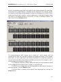
FluoroQuality analyses only a part of the whole image area. The analysed area
(sub-image) is selected in the acquisition program by the user. These subimages must be of size 64x64 pixels, with 8-bit pixel depth, and each recorded
sequence must contain 32 consecutive image frames. These image data are
denoted below by gs(i, j, k, m), where i denotes the pixel column (1 ≤ i ≤ 64), j the
pixel row (1 ≤ j ≤ 64), k the frame number (1 ≤ k ≤ 32) and m (1 ≤ m ≤ M)
identifies the image sequence. (The number of image sequences, M, is
determined in the acquisition program; values of M ≥ 40 are recommended for
keeping the bias and uncertainty small.) The subscript s = 1 for images
recorded with the signal detail in the phantom, and s = 0 for images recorded
with the detail removed.
Two- and three-dimensional discrete Fourier transformed (DFT) images
are denoted with capital letters, and the horizontal, vertical and temporal
frequencies are denoted by u, v and w, respectively: e.g., Gs(u, v) = F2[gs(i, j)] and
Gs(u, v, w) = F3[gs(i, j, k)] , where Fn[] denotes the n-dimensional DFT operation.
It is emphasized that FluoroQuality uses the symmetric normalisation
convention of DFT; therefore, the transformation differs from the DFT with the
(more commonly used) unsymmetrical normalisation convention by the factors
64⋅ 64 and 64 ⋅ 64 ⋅ 32 for the 2D and 3D cases, respectively.
The width and height (in units of length) of the analysed 64x64 pixel subimage is denoted as X and Y, respectively. However, X and Y are not actually
measured in FluoroQuality and a numerical value of 1 is used for both of them.
If the user wishes to express the spatial frequencies and the NPS in proper
units (mm-1 and mm2) the values of X and Y can be taken into account by hand
calculation: for example, the horizontal frequency u (-31 ≤ u ≤ 32) corresponds
to the spatial frequency u/X, and the 2D NPS values can be obtained by
multiplying the values calculated in FluoroQuality by XY. The temporal length
of the 32-frame image sequences is denoted as T.
22
STUK-A196
One should also note that all values in FluoroQuality are calculated in
terms of the pixel values. If the user so wishes, these values can be later
converted to correspond to some other quantities, e.g., x-ray fluence, by
applying the proper conversion factors. Such a conversion makes a difference
only in the numerical values of the average images and NPS data – the signalto-noise measures are not affected.
3.2 Average images
FluoroQuality calculates the average signal and background images (recorded
with and without the signal detail in the phantom, respectively) as
(10)
g s (i, j ) =
1
32 ⋅ M
M
32
¦¦ g (i, j, k , m) ,
m =1 k =1
s
s = {0, 1}.
The average images for the signal and background cases are shown on the
FluoroQuality display form.
3.3 The net signal and its frequency spectrum
The net signal is obtained as
(11)
∆g (i, j ) = g1 (i, j ) − g 0 (i, j )
and the spatial frequency spectrum of the signal is defined*) as
(12)
'G u , v 2
2
F2 >'g i, j @ .
The net signal image and the signal spectrum are shown on the FluoroQuality
display form.
*)
The relationship between this signal spectrum and the one used in eq. (7) is similar to the
relationship between the noise quantities R and W in eq. (14).
23
STUK-A196
3.4 The NPS of individual image frames and the spatiotemporal NPS at zero temporal frequency
The variance at each spatial frequency, R(u, v), which is related to the twodimensional NPS (see, e.g., Tapiovaara and Wagner 1993), is measured as
(13)
Rs (u, v)
ª
1
1
2
«¦ F2 >g s (i, j, k , m)@ ( M ˜ 32 1) « k ,m
M ˜ 32
¬
2
º
».
>
@
F
g
(
i
,
j
,
k
,
m
)
¦
2
s
»¼
k ,m
The two-dimensional NPS corresponding to individual frames is then
calculated as
(14)
W2 D ,s (u / X , v / Y )
XY
˜ Rs (u , v).
64 2
The measurement is made separately for both the signal (s = 1) and
background images (s = 0). When reporting the NPS, FluoroQuality uses the
value 1 for both factors X and Y. If the user wishes to normalise his/her data to
the actual size of the image, the calculated NPS-values should be multiplied
with the measured value of XY, and the spatial frequencies are obtained by
dividing the displayed (integer) values of u and v by X and Y, respectively. It is
again emphasized that the normalisation in (14) differs from some other texts
because of the DFT normalisation used; the resulting NPS is the same,
however.
Similarly, the variance of the summed 32-frame long sequences,
corresponding to the zero temporal frequency component of the 3D spatiotemporal NPS, is measured as
2
2
1
1 ª
ª
º º
ª
º
«¦ F2 «¦ g s (i, j , k , m)» (15) Rsum , s (u , v)
¦ F2 «¬¦k g s (i, j, k , m)»¼ »»
M 1 « m
M m
¬ k
¼
¬
¼
and the corresponding zero frequency component of the 3D spatio-temporal
NPS of the sequences is calculated as
(16)
. 3 D , s (u / X , v / Y , 0)
W
XYT
˜ Rsum, s (u , v).
64 2
Again, the measurement is made separately for both the signal (s = 1) and
background images (s = 0), and the value 1 is used for the factors X, Y and T in
the displayed data. Therefore, if the user wishes to normalise his/her data to
the actual size of the image and the temporal length of the sequence, the
calculated NPS-values should be multiplied with the measured value of XYT.
The spatial frequencies are obtained by dividing the (integer) values of u and v
by X and Y, respectively.
24
STUK-A196
3.5 The full spatio-temporal NPS
The full spatio-temporal NPS is calculated as
(17)
W 3 D , s (u / X , v / Y , w / T ) =
XYT
2
F3 [g s (i, j , k , m ) − g s (i, j )] .
¦
2
(M − 1) ⋅ 64 ⋅ 32 m
Again, the measurement is made separately for both the signal (s = 1) and
background images (s = 0), and the value 1 is used for the factors X, Y and T. If
the user wishes to normalise his/her data to the actual size and temporal length
of the image sequence, the calculated NPS-values should be multiplied with the
measured value of XYT, and the spatial frequencies are obtained by dividing
the (integer) values of u and v by X and Y, respectively. In displaying the NPS,
the temporal length of the image sequences is already taken into account, and
the proper temporal frequency (in Hz) is displayed on the NPS display-form.
3.6 The SNR-measures obtained by integration (analytical
biased data)
Using the measured signal spectrum and NPS, FluoroQuality estimates the
(biased) SNR2 and SNR2rate of two computational observers: the DC- and HFsuppressing observer (DCsHFs) and the prewhitening matched filter (PWMF,
the ideal observer). It should be noted that the residual noise in the average
images and NPS data make these estimates high-biased, as discussed earlier in
Chapter 2.3, and it is not advisable to use them for estimating the detectability
of the signal. The data may be useful, however, for estimating the effect of the
different detection algorithms on the resulting SNR estimate. The data are
presented as a function of the maximum included spatial frequency in the
summation, flmt.
The SNR2DCsHFs of the individual image frames is calculated as
2
(18)
2
SNRDCsHFs
( f lmt ) =
§
2·
¨
∆G (u , v) ¸¸
¦
¨
© f ≠ ( 0,0 ) or ( 0,32)
¹
½
⋅
(
R
(
u
,
v
)
+
R
(
u
,
v
)
) ∆G (u, v) 2 ,
¦ 0
1
f ≠ ( 0, 0 ) or ( 0 , 32 )
where the summation is done only over frequencies f = (u, v) where
(19)
f = u 2 + v 2 ≤ f lmt
and flmt is equal to 7, 15, 30 or not limited (-31 ≤ u, v ≤ 32).
25
STUK-A196
The ideal observer’s (biased) SNR2 is calculated as
(20)
SNR
2
PWMF
( f lmt ) =
¦
f ≤ f lmt
∆G (u , v)
2
½ ⋅ (R0 (u, v) + R1 (u , v) )
,
and again presented as a function of the maximum included frequency, flmt.
In a close analogy of the above formulae, the SNR2rate of the observers is
calculated as
2
(21)
2
SNRrate
, DCsHFs ( f lmt ) =
§
2·
¨
∆G (u , v) ¸¸
¦
¨
© f ≠( 0, 0) or ( 0,32 )
¹
2 ,
¦ ½ ⋅ (Rsum,0 (u, v) + Rsum,1 (u, v)) ∆G(u, v)
1
⋅
T
f ≠ ( 0 , 0 ) or ( 0, 32 )
and
(22)
.
∆G (u , v)
1
⋅ ¦
T f ≤ flmt ½ ⋅ (Rsum,0 (u, v) + Rsum,1 (u, v) )
2
2
SNRrate
, PWMF ( f lmt ) =
3.7 The SNR-measures obtained by integration (analytical debiased data)
As discussed by Gagne and Wagner (1998), the direct summation over the
spatial frequency channels of the estimated (biased) SNR2 spectrum results to
a biased SNR2-value. FluoroQuality calculates also a de-biased SNR2-estimate
by their theory as
(23)
2
SNRideal
,debiased ( f lmt ) =
¦ SNR
f ≤ f lmt
2
f ,debiased
,
where
§ 2 N eff ( f ) − 3 ·
∆G ( f )
2
¸⋅
−
=¨
¨ 2 N ( f ) − 2 ¸ ½ ⋅ (R ( f ) + R ( f ) ) N ( f )
eff
0
1
eff
¹
©
2
(24)
SNR
2
f , debiased
is the bias-corrected SNR2 spectrum, and Neff(f) is the effective number of
images in either the signal or background case (see the explaining text later).
26
STUK-A196
The error, σ , of SNR2ideal, debiased(flmt) is also estimated according to the
theory of Gagne and Wagner (1998) by adding the variances of each included
frequency channel
(
4(N eff ( f ) − 1)
(25)
)
2
­° 4
SNR 2f ,debiased ½°
4
2
+
⋅
+
SNR
®
¾
,
f
debiased
2( N eff ( f ) − 1) °
(2 N eff ( f ) − 3)2 (N eff ( f ) − 2) °̄ N eff2 ( f ) N eff ( f )
¿
3
σ 2 ( SNR 2f ) =
(The bias and variance at the spatial zero and Nyquist frequencies are actually
slightly different from the expressions above: see Gagne and Wagner (1998).)
In Eqs (24–25) we have used the effective number of images, Neff(f),
instead of the actual number of images. This is because for each imaging
condition there are M files of 32 frames each used in the calculation, but the 32
frames in any of the files are not necessary statistically independent because of
lag. The lag effect may depend on the spatial frequency*) and, therefore, the
effective number of images at each spatial frequency is estimated separately as
being
N eff ( f ) = M ⋅ 32 ⋅
(26)
R0 ( f ) + R1 ( f )
R0,sum ( f ) + R1,sum ( f ) .
In FluoroQuality Neff is subjected also to the condition M ≤ Neff ≤ 32·M.
The above expressions are almost similar for the calculation of the
2
SNR rate:
2
SNRrate
,ideal ,debiased ( f lmt ) =
(27)
1
T
¦ SNR
f ≤ f lmt
2
f , seq ,debiased
,
where
∆G (u , v)
2
§ 2M − 3 ·
SNR 2f ,seq ,debiased = ¨
−
¸⋅
,
© 2 M − 2 ¹ ½ ⋅ (Rsum,0 (u , v) + Rsum,1 (u, v) ) M
2
(28)
(29) σ ( SNR
2
2
f , seq
(
3
­° 4
SNR 2f ,seq ,debiased
4(M − 1)
4
2
)=
+
⋅
+
SNR
®
f
seq
debiased
,
,
2( M − 1)
(2M − 3)2 (M − 2) °̄ M 2 M
) ½°
2
¾
°¿
and M denotes the number of recorded signal or background image sequences.
There is no need to estimate an effective number instead of M, because the
sequences can be assumed to be statistically independent.
*)
Typically, the noise at low spatial frequencies is dominated by quantum noise, which is
affected by the lag in the imaging system. The noise at high spatial frequencies is often
dominated by temporally white electronic noise.
27
STUK-A196
3.8 Temporal lag
Temporal lag was evaluated in terms of the lag factor F in Tapiovaara (1993).
This factor compares the information rate in an image sequence to the
information in a single frame and shows the effective number of independent
image frames per unit time. In that paper, F was defined in terms of the DCsuppressing observer. Here, lag is reported in terms of quantities related to 1/F
and the unit of the lag-measures is s.
Three slightly different measures of lag are given in the output of
FluoroQuality. One is the lag measure related to the comparison of SNR2 in a
single frame and SNR2rate of the ideal observer
(30)
Lag PWMF =
2
SNRideal
, debiased
.
2
SNRrate
,ideal , debiased
The other one is calculated similarly to the DC/HF-suppressing observer and
the third one is obtained from the DCsHFs-observer by excluding the spatial
frequency axes (u = 0 or v = 0) from the summation:
(31)
Lag DCsHFs ,excl.axes = T ⋅
¦ ∆G (u, v)
u ≠ 0,v ≠ 0
¦ ∆G (u, v)
u ≠ 0 ,v ≠ 0 )
2
2
⋅ ½( R0 (u , v) +R1 (u, v))
⋅ ½( Rsum,0 (u, v) +Rsum,1 (u , v)) .
This last lag measure was developed in the past, when we often experienced
excessive noise on the spatial frequency axes (cross-like shape in the NPS). We
have not seen these artefacts with NPS calculations made with FluoroQuality,
however. Anyway, in our experience, this last lag measure is the most stable of
the measures presented above, and it is used in calculating the SNR2rate, DCsHFs as
will be explained in 3.10. The error (1 STD) in the lag-measure is estimated
from the expected precision of the average images and the NPS.
3.9 The DCsHFs-observer’s SNR obtained using the template
method
In addition to the analytical calculations explained above, FluoroQuality
measures the DCsHFs-observer’s SNR in the single frames by the following
method: A template is calculated from the net signal ∆g (i, j ) by first
calculating the average pixel values of its even and odd pixel rows (these
correspond to the even and odd video fields of one video frame) and subtracting
28
STUK-A196
these averages from the pixel values of the respective pixel rows of the net
signal. This results to a template whose DFT would have the value zero at
frequencies (0, 0) and (0, vmax)*). This template is calculated separately for each
image sequence file, m, by leaving this sequence out in calculating the average
image, and is denoted here as ∆g DCsHFs , m (i, j ) . This template is then crosscorrelated with each image frame in sequence m to get the DCsHFs-observer’s
conditional decision variables
(32)
D DCsHFs ( g k ,m | s ) = ¦ ∆g DCsHFs , m (i, j ) ⋅ g s (i, j , k , m) .
i, j
The SNR is then calculated from these values as shown in Eq 1.
There are also other possibilities to use the image data for the
measurement. For example, one could divide the image data in two separate
groups, and use one group for estimating the averages and the other for testing
the performance. However, this results to inefficient use of the data and
unnecessary imprecision and bias in the results. Another alternative would be
not to leave out the image data being tested from estimating the average
image; this would lead to biased results.
The error (1 STD) in the obtained SNR2 is estimated as
(33)
2
) = 2 ⋅ SNRDCsHFs ⋅
σ (SNRDCsHFs
(
(
)
)
2
SNRDCsHFs
⋅ σ 4 ( D | 0) + σ 4 ( D | 1)
2
+
N eff 2 ⋅ (N eff − 1)⋅ σ 2 ( D | 0) + σ 2 ( D | 1) 2 ,
where the effective number of images is estimated from
(34)
N eff = M ⋅
T
Lag DCsHFs ,excl.axes .
The SNR-measurement is subjected to a test of the equality of the variances of
the decision variable D with the conditions of signal present and absent; the
variances should be equal if the noise is truly signal-independent. The user is
noted if one of the variances is more than 20% larger than the other.
The measurement is also subjected to a X 2-test of the normality of the
conditional decision variables. The user is warned if the test suggests nonnormality of the data (i.e., if the value of the X 2 -variable is larger than the 1%
significance limit).
*)
To suppress only the frequency (0, 0) it is sufficient to subtract the average pixel value of
the entire net signal image. However, interlaced scanning TV-systems often exhibit
excessive noise also at the spatial frequency (0, vmax), and it is useful to suppress this
frequency as well.
29
STUK-A196
3.10 SNR2rate
The SNR2rate of the DCsHFs-observer is estimated in two ways: (i) by measuring
the SNR2 of the image sequences essentially as explained in 3.9, but by testing
images that are averaged over the whole image sequence length (32
consecutive frames) instead of testing the individual frames as was done in 3.9;
the SNR2rate is obtained by dividing the SNR2-estimate of the averaged images
by the acquisition time of the sequence, T. The other method (ii) is to estimate
the SNR2rate from the SNR in single image frames and the lag as
(35)
2
SNRrate
, DCsHFs =
2
SNR DCsHFs
.
Lag DCsHFs ,excl.axes
3.11 Bias issues of SNR measurements
As already discussed in chapter 2.3, an uncorrected measurement of SNR from
the average image and NPS data results to biased results, mainly because the
residual noise in the averaged data will be interpreted as being part of the
signal. On the other hand, the residual noise in the average images that are
used in the DCsHFs-template method of SNR-measurement (Chapter 3.9)
causes that the results from this method are low-biased: in this case, the noisy
template does not accurately correspond to the actual signal and doesn’t,
therefore, perform as well as a noiseless template would do.
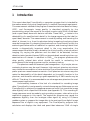
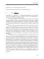
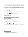
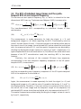
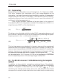
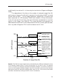
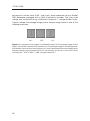
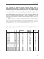
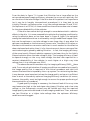
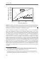
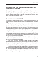
The SNR2 and SNR2rate estimates from three measurement methods ((i)
the analytical biased estimate, (ii) the analytical de-biased estimate and (iii)
the estimate from the DCsHFs-template method) are shown in Figs 1 and 2 for
0,9–3,7 mm thick PMMA-disk signals of 1 cm diameter, obtained at different
imaging conditions (varying the dose rate, the optical aperture between the
image intensifier and the TV-camera, and the use of an antiscatter grid). The
background phantom used in the measurements consisted of a 2 mm copper
plate at the x-ray tube housing and a 4,7 cm PMMA block placed on the x-ray
image intensifier. The x-ray tube voltage was 72 kV, the source-to-image
distance 108 cm and the x-ray beam size at the x-ray image intensifier
entrance plane 23 cm x 23 cm. The number of image files, M, was 40 in these
measurements (i.e., 40 image sequences of 32 consecutive frames each were
30
STUK-A196
recorded for both the signal and the background case). The “true” value of the
SNR2 for each disk at each separate imaging condition is obtained, by physical
reasoning, as the average of the measurements by methods (ii) and (iii) above
for the thickest detail at that imaging condition and scaling this SNR2 by to the
ratio of the squares of the disk thicknesses. The SNR2-estimates are shown in
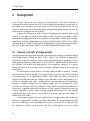
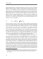
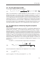
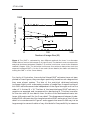
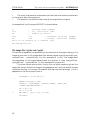
Fig. 1 and the SNR2rate-estimates in Fig. 2.
100
2
SNR -estimate
1000
10
Biased PWMF-estimate (Ch. 3.6)
De-biased PWMF-estimate (Ch. 3.7)
Template method (Ch. 3.9)
1
1
10
100
1000
2
SNR
Figure 1. The estimates of the SNR2 in single image frames as measured by three
methods (Chapters 3.6, 3.7 and 3.9). The data correspond to the detectability of 1 cm
diameter PMMA disks of various thicknesses in various imaging conditions. Number of
signal and background image files M = 40. The data are plotted against the true SNR2 of
the details.
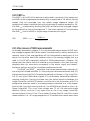
31
STUK-A196
2
SNR rate- estimate (1/s)
10000
1000
Biased PWMF-estimate (Ch. 3.6)
100
De-biased PWMF-estimate (Ch. 3.7)
Template method (Ch. 3.10)
10
10
100
1000
10000
2
rate (1/s)
SNR
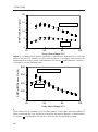
Figure 2. The estimates of the SNR2rate as measured by three methods (Chapters 3.6, 3.7
and 3.10). The data correspond to the detectability of 1 cm diameter PMMA disks of
various thicknesses, in various imaging conditions. Number of signal and background
image files M = 40. The data are plotted against the true SNR2rate of the details.
In the figures it is seen that the uncorrected (biased) SNR-estimates suffer
increasingly from the bias when the SNR gets smaller; therefore, these results
are not of much use. The template-method-estimates are somewhat low-biased
at very low SNR’s, as expected, and the de-biased SNR estimates seem to get
slightly high-biased at low SNR’s, in spite of the bias-correction.
The de-biased analytical SNR-data include also a few outliers, whose
value is notably higher than expected. These outliers are characterised by their
signal spectra including more power in their high spatial frequency region than
would be expected from the actual low-frequency signal used – it seems that in
some cases the averaging process of the signal and background images has not
cleaned image noise in the average images as well as would be expected by the
number of images. These outliers stood out also in the analytical SNRcalculation results by the strong dependence of their SNR2-values on the
maximum included frequency, flmt. A possible method of reducing the bias of
(truly) low-frequency signal details is then to use the SNR-estimates based on
32
STUK-A196
a sufficiently low value of flmt in the analytical calculation (Gagne and Wagner
1998).
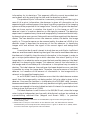
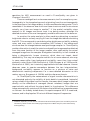
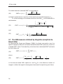
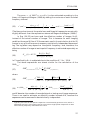
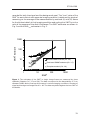
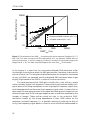
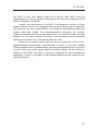
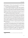
The dependence of the bias on the number of analysed image files (M)
can be seen in figures 3 and 4 which represent the estimates of SNR2 in single
frames and the SNR2rate of the image sequences, respectively. The data have
been measured for 1 cm diameter PMMA disk details of three thicknesses:
0 mm, 0,9 mm and 3 mm thick, (the zero thickness corresponds to no actual
signal in the image: true SNR=0). The same phantom and geometry as
described above was used. In the measurements the anti-scatter grid was used,
the x-ray tube voltage was 72 kV and the tube current 0,7 mA.
100
3 mm detail
Analytical de-biased
SNR^2(No signal)
Analytical de-biased
SNR^2(0,9 mm signal)
10
0,9 mm detail
Template method
SNR^2(0,9 mm signal)
Analytical de-biased
SNR^2(3 mm signal)
2
SNR -estimate
Template method
SNR^2(No signal)
Template method
SNR^2(3 mm signal)
1
SNR^2(true, 0,9 mm
signal)
No detail
SNR^2(true,3 mm
signal)
0,1
10
100
1000
Number of image files (M)
Figure 3. The SNR2 of single image frames, estimated by two different methods for three
1 cm diameter PMMA disks of various thicknesses (0, 0,9 and 3 mm). The dashed
curves correspond to analytical de-biased estimates (Chapter 3.7) and the continuous
curves to the template method (Chapter 3.9). The horizontal continuous lines without
data points show the expected unbiased SNR2-value for the 3 mm and 0,9 mm detail
(the latter calculated by scaling the SNR2 of the 3 mm datum).
33
STUK-A196
1000
2
SNR rate-estimate (1/s)
3 mm detail
100
0,9 mm detail
10
No detail
1
10
100
Number of image files (M)
1000
Figure 4. The SNR2rate, estimated by two different methods for three 1 cm diameter
PMMA disks of various thicknesses (0, 0,9 and 3 mm). The dashed curves correspond to
analytical de-biased estimates (Chapter 3.7) and the continuous curves to the template
method (Chapter 3.10). The horizontal continuous lines without data points show the
expected unbiased SNR2rate for the 3 mm and 0,9 mm details (the latter calculated by
scaling the SNR2rate of the 3 mm datum).
For clarity of illustration, the analytical biased SNR2 estimates have not been
plotted in these figures; they were again positively biased to such a degree that
they were almost useless. The bias of the analytical de-biased estimate
increases slightly with a decreasing number of image files; the positive bias of
this SNR2 estimate seems to be independent of the signal strength and is of the
order of 3–4 when M = 10. The bias of the template-based SNR2-estimate is
negative, as expected, and increases with a decreasing M. This bias is smaller
for the zero and 0,9 mm details than the bias of the de-biased estimate, but
larger (although small) for the 3 mm detail. The disagreement between the debiased SNR2 estimate and the template method SNR2 estimate of the 0,9 mm
detail is in accordance with Figure 1 and suggests that even M=160 may not be
large enough to remove the bias of very faint details. One possibility to measure
34
STUK-A196
the SNR2 of such thin details might be to derive their SNR2 from the
measurement of a thicker detail by scaling with the ratio of the squares of the
detail thicknesses, if possible.
Overall, the conclusions of the SNR2rate estimates are similar to those
above; the bias is minor for reasonably strong signal details and an important
issue only for very faint signal details. The analytical de-biased estimates are
slightly positively biased, the template-method estimates are slightly
negatively biased, and the bias decreases with an increasing number of image
samples. In this case, however, the bias of the template-matching estimate
appears to be lowest for all the details when M is low.
Based on the above results and our earlier experience, the DCsHFstemplate-based measurement method seems to result in the most reliable
SNR-estimates from the measurement alternatives considered here. The use of
a low M and a very weak signal detail should be avoided. The bias (which is
evident at low SNR2 and SNR2rate values for moderate M) could perhaps be
reduced by using the average of the template-based and the analytical debiased estimates.
35
STUK-A196
4
SNR2rate and detail visibility
For static radiographs, it is often said that a SNR of 3–7 (SNR2 ~ 9–50) is
needed for a detail to be visible. This is, however, just a rule of thumb trying to
relate the SNR with visibility*). Actually, there is no detectability threshold, but
the detail turns from not visible to clearly visible through a continuosly
improving detection certainty when the SNR is increased.
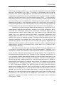
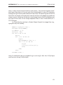
The statistical efficiency F = (d’)2/SNR2ideal of humans is often found to be
of the order of 50%: then, a human observer who is presented images with a
detail of, say, SNRideal = 2 would obtain a d’~ 1.41 and achieve a 84 % probability
of a correct answer in a 2AFC test, or a 39 % probability in a 16-AFC test (see
figure 5 for the relationship between d’ and the probability of a correct
response in some MAFC tests). Some authors have equated the criterion of
1
P(Correct response)
2AFC
0,8
4AFC
16AFC
0,6
128AFC
0,4
512AFC
0,2
0
0
2
4
6
d'
Figure 5. The relationship between the observer’s signal-to-noise ratio at the decision
level (d’) and the probability of a correct response in some MAFC tests.
*)
36
The use of SNR thresholds has been criticized by many researchers, e.g., Burgess (1983),
who also pointed out that Rose had suggested SNR threshold values (denoted by k) in the
range from 3 to 5. After his criticism Burgess writes “…However if you insist on using the
Rose model it is suggested that you use values of “k” in the range from 5 to 10 for simple
detection and 15 to 20 for signal identification tasks”.
STUK-A196
detectability with the condition of 50 % correct responses in an 18-AFC test,
which corresponds to d’ = 1,78. Using the estimate of F = 50 %, this would
correspond to the detectability of signals with SNR > 2.5.
In fluoroscopy the “threshold contrast” (i.e. the lowest contrast detail
that the observer subjectively judges as perceivable) is likely to depend on
several factors in addition to the SNR2rate. These factors may include, e.g., the
instructions given to the observers, the design of the test object, the displayed
contrast, the properties of image noise, the allowed observation time and any
background non-uniformity. One should also note that the inter- and
intraobserver variability in visibility threshold tests is large: the “threshold” is
difficult to define and keep, and may therefore have a different meaning to
different observers and to a given observer at various times.
In the human observer tests that we have made, we have found an
average SNR2rate for the observers declaring a detail in a noisy fluoroscopic
image as just visible*) to be around 60 s-1. This “threshold SNR2rate” did not seem
to be independent of the noise (or dose) level, however, but increased with the
dose rate (i.e., decreasing noise): the average “threshold SNR2rate” was 87 s-1 for
a two-fold dose rate and 140 s-1 for a four-fold dose rate, compared to the lowest
dose rate in the tests. So, the observers’ visibility threshold did not improve as
much as would be expected by SNR reasoning. The threshold SNR2rate
variability between the observers in these tests was large, about 40%, and one
should consider these “thresholds” only as typical values. Nevertheless, these
figures may give a feel for the SNR2rate magnitude required for a subjective
sensation of visibility.
We also made 16-AFC tests at two of the lowest dose levels referred to
above. The SNR2rate of the test detail was equal to 19 s-1 at the lowest dose rate
and equal to 40 s-1 at the two-fold dose rate level (i.e., the SNR2rate of the test
details were about one third or one half of the SNR2rate of the details that the
observers reported as just visible in the threshold-experiment). The square of
the observers’ mean detectability index, d’ 2, was 6.6 and 12.4 in these imaging
conditions, respectively. These results are compatible with the assumption that
the observers’ d’2 is proportional to the SNR2rate. This suggests that in the
“threshold” test the observers evaluated the detail contrast to be more
important than was actually the case in the controlled detectability test.
*)
The observers were instructed “to try to see through the noise but without needing to
guess”.
37
STUK-A196
It is problematic to evaluate the statistical efficiency of the human
observers in fluoroscopy because the available SNR increases with fluoroscopy
time (and the efficiency would be very low), but one can think of the ratio teff = d’
2
/ SNR2rate as depicting the effective time that a human has integrated the
information from a live image sequence. This interpretation should not be
taken literally, however: the detection times in the 16AFC tests above were
very long, from about 30 s to several minutes for each single observation.
Anyway, the obtained result of teff § 1/3 s may be a useful rule of thumb for
interpreting the meaning of SNR2rate from a human observer standpoint. This
rule seems to apply even to the “SNR threshold” tests mentioned above; the
2
“perceived SNR thresholds”, teff ⋅ SNRrate
, range from 4.4 to 6.9 and are in
,thresh
good agreement with values quoted for static images.
It is however noted that we have earlier (Tapiovaara 1997) found
a relatively high efficiency for human observers detecting static low-contrast
details in dynamic noise. These earlier measurements were made using the
2AFC method and finite-length image sequences, which were replayed in
a continuous loop. Interpreting the data from that study in a similar way as is
done here would suggest an effective information integration time of at least
0,8 s, given that the display contrast is optimal. We do not presently know the
reason for this difference between our present and earlier data, but suspect
that it could be due to the much easier decision task in the 2AFC experiment
compared to the 16-AFC experiment used here – having only two possible
signal locations near each other does not place similar demands on memory as
signal detection from several alternatives in a large image area does.
38
STUK-A196
5 An example of using FluoroQuality for imaging
technique optimisation
In this chapter we give an example of how FluoroQuality can be used for
optimising the imaging technique for a given detection task*). This example is
related to interventional imaging, and considers the detectability of an USCI
5F catheter (type 08LF0878) in an about 25 cm thick patient. The measurement
is easy and quick; the measurements described here were made in less than
two hours.
The patient-simulating phantom consisted of several slabs, whose total
thicknesses were 20.5 cm polymethyl methacrylate (PMMA), 4.3 mm
aluminium and 5 mm water; the lateral extent of the phantom was 24 cm x
24 cm. A 13 mm piece of the catheter was filled with water and immersed in the
water layer on top of the phantom, in order to mimic its contrast within a vein
(in this case without any contrast material). The distance between the x-ray
tube focal spot and the image intensifier entrance plane was 110 cm, and the
field size at the image intensifier entrance plane was 20 cm x 20 cm. The
distance between the x-ray tube focal spot and phantom top was 87 cm.
The x-ray equipment used for the measurements consisted of a Valmet
BR 2001 three-phase 12-pulse high-voltage generator, a rotating anode x-ray
tube (Comet DI 10 HS 22/52-150, total filtration without any added filter
2.1 mm Al), a Philips Imagica 23 cm image intensifier and an XTV-11 video
chain with a low-lag Vidicon (Newvicon) pick-up tube operated in the 625 lines/
frame interlaced scan mode. A stationary antiscatter grid (strip density 44 line
pairs cm-1, grid ratio 10:1, carbon fibre cover plates, focusing distance 1 m) was
located in front of the image intensifier entrance plane.
The phantom was imaged in the fluoroscopic mode, using various
imaging conditions (with and without an added 0.25 mm Cu-filter, several xray tube voltages). The x-ray tube voltage and current were chosen manually
but the gain in the video chain was automatically controlled. The fluoroscopic
sequences were recorded both with and without the signal detail (13 mm piece
of the USCI 5F catheter) in the analysed image area by using a Matrox Genesis
LC frame grabber board and the NoiseAcquisition-program (see Appendix A).
The image sequences were analysed with the FluoroQuality-program. The
*)
The optimum imaging conditions are defined as those that result to the lowest dose in the
patient for a specified image quality.
39
STUK-A196
entrance air kerma rates (EAK, free-in-air) were measured using a Radcal
9015 dosemeter equipped with a 10x5-6 ionisation chamber. The x-ray tube
voltage was monitored using a Machlett Dynalyzer II voltage divider chain.
Figure 6 shows the average images and a sample image frame in one of the
imaging conditions.
(a)
(b)
(c)
Figure 6. An example of the images in the detection task. (a) The average image for the
signal; the catheter located in the phantom. (b) The average image for the background;
the catheter removed from the phantom. (c) A one-frame sample from the image series
with the catheter in the phantom. 65 kV, 5.7 mA, filtration 2.1 mm Al + 0.25 mm Cu, EAK
3.93 mGymin-1, SNR2rate 891 s-1, SNR of single frames 10.7.
40
STUK-A196
Table 1 shows the measured imaging conditions together with the
measurement results of SNR2rate and dose rate. (Note that the data have not
been acquired by using the automatic dose rate control, and the dose rate does
not, therefore, decrease with an increasing tube voltage. This does not affect
our analysis here, because the system is well quantum noise limited; this can be
seen, e.g., from the data at 2.1 mm Al filtration, 65 kV; 0.3 and 2.1 mA.) The rate
of the effective dose was calculated with the PCXMC -program (Tapiovaara et
al. 1997). The effective dose data given in Table 1 correspond to the PAprojection in a cardiological procedure of an obese patient (174 cm height and
105 kg mass).
Figures 7 and 8 show the dose-to-information conversion factors
2
(SNR rate/dose rate) calculated from the data and corresponding to the air
kerma rate and the rate of effective dose, respectively. The data have been
plotted as a function of the x-ray tube voltage for both filter choices.
Table I. Measurement data for the optimisation example of detecting a catheter in the
heart of a 25 cm thick patient. SNR2rate is calculated as the average of two estimates
(Chapters 3.7 and 3.10)
Total filtration
kV
mA
2.1 mmAl
2.1 mmAl
2.1 mmAl
2.1 mmAl
2.1 mmAl
2.1 mmAl
2.1 mmAl
2.1 mmAl
2.1 mmAl
2.1 mmAl
2.1 mmAl
2.1 mmAl
2.1mmAl+0.25 mmCu
2.1mmAl+0.25 mmCu
2.1mmAl+0.25 mmCu
2.1mmAl+0.25 mmCu
2.1mmAl+0.25 mmCu
2.1mmAl+0.25 mmCu
2.1mmAl+0.25 mmCu
2.1mmAl+0.25 mmCu
2.1mmAl+0.25 mmCu
2.1mmAl+0.25 mmCu
45
50
55
60
65
65
70
75
80
85
90
95
50
55
60
65
70
75
80
85
90
95
6.3
2.5
1.0
0.5
0.3
2.1
1.1
0.7
0.5
0.5
0.5
0.5
6.3
6.3
6.3
5.7
3.7
2.3
1.5
1.1
0.8
0.6
Air kerma rate
(mGy/min)
11.0
5.75
2.84
1.70
1.18
8.55
5.15
3.68
2.90
3.22
3.55
3.90
1.42
2.22
3.20
3.93
3.36
2.61
2.09
1.84
1.56
1.39
Effective
dose rate
(PSv/min)
86.5
56.2
33.2
23.2
18.3
133
90.0
71.8
62.6
76.1
91.0
107
31.8
58.8
97.3
134
126
107
92.4
86.5
77.2
71.8
2
SNR rate
(1/s)
574
417
273
165
121
792
466
331
260
249
280
290
310
531
747
891
693
505
350
305
209
176
41
STUK-A196
15
2,1 mm Al + 0,25 mm Cu
10
2
SNR rate/EAKrate (1/µGy)
20
5
2,1 mm Al
0
40
60
80
100
X-ray tube voltage (kV)
Figure 7. The dose-to-information conversion coefficient for detecting a 13 mm long
piece of the USCI 5F catheter in a 25 cm thick patient. In this figure, the entrance air
kerma rate (free-in-air) is used. x: total filtration 2.1 mm Al, : total filtration 2.1 mm Al +
0.25 mm Cu, curves fitted by hand.
2
SNR rate/Eff.Doserate (1/mSv)
800
2,1 mm Al + 0,25 mm Cu
600
400
2,1 mm Al
200
0
40
60
80
100
X-ray tube voltage (kV)
Figure 8. The dose-to-information conversion coefficient for detecting a 13 mm long
piece of the USCI 5F catheter in a 25 cm thick patient. In this figure, the rate of effective
dose is used and the x-ray projection is heart PA (see text for details). x: total filtration
2.1 mm Al, : total filtration 2.1 mm Al + 0.25 mm Cu, curves fitted by hand.
42
STUK-A196
From the data in figure 7 it is seen that filtration has a large effect on the
entrance dose-based imaging efficiency, whereas the curves are relatively flat
as a function of the tube voltage. If the skin dose of the patient is of importance
(as it may be in lengthy interventional procedures) it is then best to use
a highly filtered x-ray beam and an x-ray tube voltage between 50 and 70 kV
(the optimum is at 55 kV). At these conditions the entrance dose rate is lowest
for the given detectability of the catheter.
If the skin dose cannot be high enough to cause deterministic radiation
effects in the skin, it is more reasonable to optimise the imaging conditions by
using the effective dose, as has been done in figure 8. Again, the optimum
among the tested alternatives is achieved by using the additional copper filter,
but now the optimum x-ray tube voltage is even lower than it was when the
optimum was based on the entrance air kerma rate. The effect of filtration on
the dose-to-information conversion coefficient is much weaker for the effective
dose rate-based evaluation than it is for the entrance air kerma rate-case. Not
much advantage is gained by adding filtration – in fact, the imaging efficiency
of the more heavily filtered radiation appears to be lower than for the lightly
filtered radiation when the tube voltage is high. The imaging efficiency is seen
to depend strongly on the x-ray tube voltage; the dose rate required for a
constant detectability of the catheter is much higher at a high x-ray tube
voltage than it is at voltages near 50 kV.
The above discussion considers only the imaging efficiency (SNR2rate/dose
rate). For an actual optimisation of imaging conditions one needs also to specify
the image quality that is required in the clinical procedure and take into
account the constraints imposed by the x-ray system. For minimising the dose,
it may be even more important to keep the image quality as low as is sufficient
than to work at the exactly optimum imaging efficiency conditions (of course,
however, the quality must be high enough to ensure the proper performing of
the examination or procedure).
If good-quality imaging is necessary, the thermal load of the x-ray tube
may become too high at the technique using heavy filtration and a low tube
voltage, or the fluoroscopic current may be limited such that the required
image quality cannot be achieved at these imaging conditions. Then, one must
use less filtration or a higher tube voltage than the optimum efficiency
conditions would suggest.
43
2
Maximum SNR rate at 6,3 mA (1/s)
STUK-A196
4000
3500
2,1 mm Al
3000
2500
2000
1500
1000
2,1 mm Al + 0,25 mm Cu
500
0
40
60
80
100
X-ray tube voltage (kV)
Figure 9. The SNR2rate that could be expected at a tube current of 6,3 mA (the maximum
for the x-ray equipment used in the measurement), as based on the data in Table and the
quantum noise limited behaviour of the imaging system. x: total filtration 2.1 mm Al, :
total filtration 2.1 mm Al + 0.25 mm Cu, curves fitted by hand.
Figure 9 shows an estimate of the maximum SNR2rate in our x-ray system at
each tube voltage and filtration (the maximum tube current in our x-ray
system is 6.3 mA). The estimate is based on the data in Table and assumes that
our imaging chain is quantum noise limited. Now, if the required image quality
would correspond to an SNR2rate of 1500/s, for example*), it would be better to
image the patient without the copper filter, because the copper filter would
require a tube voltage of at least 80 kV in order to achieve the required image
quality. The efficiency is low at such high voltages, and the aluminium-filtered
system operating at 55 kV would in this case allow an about 50% lower effective
dose rate (see fig. 8). The actual optimum condition of this example would
require a filtration between the two examples here**): the optimum filter would
be the thickest filter that allows the use of an x-ray tube voltage near 50–55 kV.
If we could use a higher power x-ray system the optimum filter thickness would
be larger.
*)
This would be a high quality fluoroscopic image: roughly, discarding effects of resolution,
even the SNR2rate for a 1 mm piece of the catheter would be equal to about 1500/13 = 115,
which suggests easy detectability of catheter details of such size.
**)
The lower filtration in this example is below the minimum allowed filtration of medical xray equipment. The use of such filters is not suggested: a system working between the two
filter examples considered would be the optimal choice here.
44
STUK-A196
6
Acknowledgements
This work was partly funded by the European Commission’s 5th Framework
Programme (1998–2002), Nuclear fission and Radiation Protection Contract,
DIMOND III (FIGM-CT-2000-00061). This report is the sole responsibility of
the author and does not reflect the opinion of the European Commission or
STUK. The European Commission or STUK are not responsible for any use
that might be made of data appearing in this report.
45
STUK-A196
7
References and further reading
Barrett HH and Swindell W, Radiological Imaging, Volumes I and II, Academic
Press, New York, 1981.
Barrett HH and Myers K, Foundations of Image Science: Mathematical &
Statistical Foundations, John Wiley and Sons, to be published 2003.
Beutel J, Kundel H, Van Metter R (eds.), Handbook of Medical Imaging, Vol 1:
Medical Physics and Psychophysics, SPIE, Bellingham 2000.
Bochud FO, Valley J-F, Verdun FR, Hessler C and Schnyder P, Estimation of the
noisy component of anatomical backgrounds, Med.Phys. 26, 1365–1370, 1999.
Brown DG, Insana MF and Tapiovaara M, Detection performance of the ideal
decision function and its McLaurin expansion: Signal position unknown,
J.Acoust.Soc.Am. 97, 379–398, 1995.
Burgess AE, Observer performance testing for medical imaging, Notes for
A.A.P.M. refresher course – August 1983.
Burgess AE, Comparison of receiver operating characteristic and forced choice
observer performance methods, Med.Phys. 22, 643–655, 1995.
Burgess AE, Wagner RF, Jennings RJ and Barlow HB, Efficiency of human
visual signal discrimination, Science 214, 93–94, 1981.
Burgess AE, Jacobson FL and Judy PF, Lesion detection in digital
mammograms, Proc.SPIE 4320, 555–560, 2001a.
Burgess AE, Jacobson FL and Judy PF, Human observer detection experiments
with mammograms and power-law noise, Med.Phys. 28, 419–437, 2001b.
Cahn RN, Cederström B, Danielsson M, Hall A, Lundqvist M, Nygren D,
Detective quantum efficiency dependence on x-ray energy weighting in
mammography, Med.Phys. 26, 2680–2683, 1999.
Chakraborty DP, Physical measures of image quality in mammography, Proc.
SPIE 2708, 179–185, 1996.
46
STUK-A196
Chakraborty DP, Computer analysis of mammography phantom images
(CAMPI): An application to the measurement of microcalcification image
quality of directly acquired digital images, Med.Phys. 24, 1269–1277, 1997a.
Chakraborty DP, Comparison of computer analysis of mammography phantom
images (CAMPI) with perceived image quality of phantom targets in the ACR
phantom, Proc. SPIE 3036, 160–167, 1997b.
Chakraborty DP, Sivarudrappa M and Roehrig H, Computerized measurement
of mammographic display image quality, Proc. SPIE 3659, 131–141, 1999a.
Chakraborty DP, Effect of antiscatter grid and target/filters in full-field digital
mammography, Proc. SPIE 3659, 878–885, 1999b.
Cunningham IA, Moschandreou T, Subotic V, Detective quantum efficiency of
fluoroscopic systems: the case for a spatial-temporal approach (or, does the
ideal observer have infinite patience?), Proc. SPIE 4320, 479–488, 2001.
Dainty JC and Shaw R, Image Science, Academic Press. London, 1974.
Dobbins JT III, Effects of undersampling on the proper interpretation of
modulation transfer function, noise power spectra, and noise equivalent
quanta of digital imaging systems, Med.Phys. 22, 171–181, 1995.
Dobbins JT III, Ergun DL, Rutz L, Hinshaw DA, Blume H and Clark DC,
DQE(f) of four generations of computed radiography acquisition devices,
Med.Phys. 22 1581–1593, 1995.
Fujita H, Ueda K, Morishita J, Fujikawa T,Ohtsuka A and Sai T, Basic imaging
properties of a computed radiographic system with photostimulable phosphors,
Med.Phys. 16, 52–59, 1989.
Fukunaga K, Introduction to Statistical Pattern Recognition, Academic Press,
New York 1972.
Gagne RM and Wagner RF, Prewhitening matched filter: practical
implementation, SNR estimation and bias reduction, Proc. SPIE 3336, 231–
242, 1998.
47
STUK-A196
Gagne RM, Myers KJ and Quinn PW, Effect of shift invariance and stationarity
assumptions on simple detection tasks: spatial and spatial frequency domains,
Proc. SPIE 4320, 373–380, 2001a.
Gagne RM, Boswell JS, Myers KJ and Peter G, Lesion detectability in digital
radiography, Proc. SPIE 4320, 316–325, 2001b.
Goldman LW, Fluoroscopic performance tests using a portable computer/frame
grabber: Wiener spectra measurements, Med. Phys. 20, 117–127, 1992.
Green DM and Swets JA, Signal Detection Theory and Psychophysics, John
Wiley and Sons, New York, 1966.
Hanson KM, Variations in task and the ideal observer, Proc. SPIE 419, 60–67,
1983.
ICRU Report 41, Modulation Transfer Function of Screen-Film Systems,
International Commission on Radiation Units and Measurements, 1986.
ICRU Report 54, Medical imaging – the assessment of image quality,
International Commission on Radiation Units and Measurements, 1996.
Kotre CJ, The effect of background structure on the detection of low contrast
objects in mammography, Br. J. Radiol. 71,1162–1167, 1998.
Loo L-ND, Doi K, and Metz CE, A comparison of physical image quality indices
and observer performance in the radiographic detection of nylon beads,
Phys.Med.Biol. 29, 837–856, 1984.
Marshall NW, The practical application of signal detection theory to image
quality assessment in x-ray image intensifier-TV fluoroscopy, Phys.Med.Biol.
46, 1631–1649, 2001.
Marshall NW, Kotre CJ, Robson KJ and Lecomber AR, Receptor dose in digital
fluorography: a comparison between theory and practice, Phys.Med.Biol. 46,
1283–1296, 2001.
Martin CJ, Sharp PF and Sutton DG, Measurement of image quality in
diagnostic radiology, Applied Radiation and Isotopes 50, 21–38, 1999.
48
STUK-A196
Metz CE, Wagner RF, Doi K, Brown DG, Nishikawa RM, Myers KJ, Toward
consensus on quantitative assessment of medical imaging systems, Med. Phys.
22, 1057–1061, 1995.
Moy JP, Signal-to-noise ratio and spatial resolution in x-ray electronic imagers:
is the MTF a relevant parameter?, Med.Phys. 27, 86–93, 2000.
Myers KJ and Barrett HH, Addition of a channel mechanism to the idealobserver model, J.Opt.Soc.Am.A 4, 2447–2457, 1987.
Myers KJ, Rolland JP, Barrett HH and Wagner RF, Aperture optimization for
emission imaging: effect of a spatially varying background, J.Opt.Soc.Am.A
7,1279–1293, 1990.
Pineda AR and Barrett HH, What does DQE say about lesion detectability in
digital radiography?, Proc. SPIE 4320, 561–569, 2001.
Siewerdsen JH, Antonuk LE, El-Mohri Y, Huang W and Cunningham IA,
Signal, noise power spectrum, and detective quantum efficiency of indirectdetection flat-panel imagers for diagnostic radiology, Med.Phys. 25, 614–628,
1998.
Siewerdsen JH, Cunningham IA and Jaffray DA, A framework for noise-power
spectrum analysis of multidimensional images, Med. Phys. 29, 2655–2671,
2002.
Smith WE and Barrett HH, Hotelling trace criterion as a figure of merit for the
optimization of imaging systems, J.Opt. Soc.Am.A 3, 717–725, 1986.
Tapiovaara MJ, SNR and noise measurements for medical imaging: II.
Application to fluoroscopic x-ray equipment, Phys.Med.Biol. 38, 1761–1788,
1993.
Tapiovaara MJ, Efficiency of low-contrast detail detectability in fluoroscopic
imaging, Med.Phys. 24, 655–664, 1997.
Tapiovaara MJ and Wagner RF, SNR and DQE analysis of broad spectrum xray imaging, Phys. Med.Biol. 30, 519–529, 1985 (Corrigendum : Phys.Med.Biol.
31, 195).
49
STUK-A196
Tapiovaara MJ and Wagner RF, SNR and noise measurements for medical
imaging: I. A practical approach based on statistical decision theory,
Phys.Med.Biol. 38, 71–92, 1993.
Tapiovaara MJ, Lakkisto M and Servomaa A, PCXMC – A PC-based Monte
Carlo program for calculating patient doses in medical x-ray examinations,
Report STUK-A139, 1997.
Tapiovaara MJ, Sandborg M and Dance DR, A search for improved technique
factors in paediatric fluoroscopy, Phys.Med.Biol. 44, 537–559, 1999.
Tapiovaara MJ, Servomaa A, Sandborg M and Dance DR, Optimising the
imaging conditions in paediatric fluoroscopy, Rad.Prot.Dosim. 90, 211–216,
2000.
van Trees HL, Detection, Estimation, and Modulation Theory, John Wiley and
Sons, New York 1968.
Wagner RF, Low-contrast sensitivity of radiologic, CT, nuclear medicine, and
ultrasound medical imaging systems, IEEE Transactions on Medical Imaging
MI-2, 105–121, 1983.
Wagner RF, Characteristic images emerging from recent SPIE medical image
symposia, Proc. SPIE 767, 138–141, 1987.
Wagner RF and Brown DG, Unified SNR analysis of medical imaging systems,
Phys.Med.Biol. 30, 489–518, 1985.
Wagner RF, Beiden SV and Campbell G, Multiple-reader studies, digital
mammography, computer-aided diagnosis – and the Holy Grail of imaging
physics (I), Proc. SPIE 4320, 611–618, 2001.
Whalen AD, Detection of Signals in Noise, Academic Press, New York, 1971.
50
STUK-A196
APPENDIX A: F LUORO Q UALITY ( V . 2.0) U SER ’ S G UIDE
General
FluoroQuality can be used for the measurement of the quality of fluoroscopic
image sequences. These sequences need first be recorded digitally by a PC/
frame grabber system using suitable software, or reformatted from the
digitally stored image sequence data of the x-ray imaging system*). The
FluoroQuality program then calculates and displays the SNR of single image
frames, the SNR2rate of the acquired image sequences, the lag, and the spatiotemporal NPS for the acquired image data. The program also displays the
average image for the signal and background situations, the net signal, the
SNR2- and SNR2rate -spectra, and can be used for visualising the acquired image
data.
The signal detail need not be located in a homogeneous phantom – in
principle, also an anatomic phantom may be used. However, strong background
structures in the phantom may violate the assumption of noise stationarity and
therefore make the NPS-measurements uncertain. Strong phantom structures
may also make the detectability of the signal detail highly dependent on the
actual location of the detail in the phantom, and therefore achieving a good
repeatability of SNR-results may be difficult. Therefore, we recommend using
a homogeneous phantom for most measurement applications. For typical
applications, the signal detail should be strong enough for obtaining accurate
results (see Ch. 3.11), but its contrast should be not too high in order to make
the noise too much signal-dependent or the SNR-results dependent on the
linearity of the imaging system and frame grabber.
The present version (FluoroQuality 2.0) is compatible with the image
data acquired using the program “Filetall” (developed in STUK for the Data
Translation DT3852 frame grabber card) or “NoiseAcquisition” (developed by
Olander and Sandborg in Linköping University Hospital for the Matrox
Genesis-LC frame grabber board). These programs require the user to define a
six-character name for the data. In this manual this name is denoted as
“xyzxyz”.
*)
Requirements for the data are given in Appendix D.
51
STUK-A196
F LUORO Q UALITY ( V . 2.0) U SER ’ S G UIDE APPENDIX A
Hardware and software requirements
FluoroQuality runs under 32-bit Windows operating systems (Windows 95/98/
NT/2000/XP). The memory requirement depends on the operating system, but
is 64 MB RAM for a PC operated under Windows NT4 (we suggest however a
minimum of 128 MB). The PC also needs sufficient hard disk space to store the
image data (about 10,3 MB for each measurement comprising of 40 background
and 40 signal datafiles) and the analysed data (1,37 MB for each measurement)
that the user wishes to keep.
In order to keep the computation times reasonably short, one should use
a fast PC. 233 MHz is a suggested minimum clock frequency.
Installation of the program
The program is installed by running the setup.exe -program of the
FluoroQuality Installation Diskette. The program can be installed in any
folder*). The setup program creates also a subfolder “\AnalysedData” which is
used for saving the data that the program calculates. Also a subfolder
“\ImageData” is created; it is intended to be the folder where the image data
are saved by the acquisition program. When the analysing calculation is
started, the program first tries to look for image data in the folder
“\ImageData”, if such a folder exists. If not, the file open-dialog window is set to
the program-containing folder and the user locates the data him/herself.
The setup -program will add a shortcut to the FluoroQuality in the
“Programs” -menu. For an even more easy access to the program, you may
create a shortcut to the FluoroQuality20.exe-file on your desktop.
*)
52
If used with the above mentioned image data acquisition programs, the
FluoroQuality20.exe-file is most conveniently installed in the folder ‘X:\Koe’. In this case it
is handy to delete the subfolder ‘\ImageData’: then the data search will begin directly in the
data folder used by these acquisition programs (X:\Koe).
APPENDIX A F LUORO Q UALITY ( V . 2.0) U SER ’ S G UIDE
STUK-A196
Using the program
Buttons
When started, the program displays the Analysis-form (below). The form has
nine buttons and other functions.
53
STUK-A196
F LUORO Q UALITY ( V . 2.0) U SER ’ S G UIDE APPENDIX A
•
The Compute data -button is used for analysing the image data
(computation of results). When clicked, an open-dialog window is shown, where
the user may choose one or several image data series (indicated by their
parameter-file name xyzxyzPM.dat. Several files can be chosen by using the
Ctrl- or Shift-keys). When clicked OK, the program calculates the analysis data
for all of the chosen image series. If the Calculate spatiotemporal NPS checkbox is checked, the program calculates these data as well. Calculating
spatio-temporal NPS data is not necessary if the user is only interested in SNR
measurements.
The SNR calculation is not performed if the data have already been
analysed; i.e., if the AnalysedData-folder already contains the file xyzxyz.txt
(the summary file of SNR-data). The NPS-calculation is not done if the
AnalysedData folder already contains the files xyzxyzbg.spt and xyzxyzsg.spt
(the spatio-temporal NPS for the background and signal image series,
respectively) or if the NPS-calculation check-box is unchecked.
The calculation can be stopped by clicking the Halt -button at any time
when the button is enabled. The remaining data can be analysed later by
choosing the same set of PM-files for computation.
•
The Retrieve data -button is used for examining data that have already
been analysed. When clicked, an open-dialog window is shown, where the user
can choose one of the data sets that have been analysed earlier (files indicated
by their analysed data file name xyzxyz.txt). The images in the Analysis-form
will be updated and the xyzxyz.txt file is shown in the memo-window.
•
The View images -button can be used for viewing the original image
data series (if they haven’t been deleted from the computer). The data can be
viewed either as individual frames or as a continuous loop with an userspecified frame refresh interval (specified in milliseconds). The average signal
image or background image can be subtracted from the images, which may, for
example, help in recognising jitter or background-structure problems in the
image data. Note that any image series can be chosen for viewing. However, the
subtracted average is always from the image set identified in the caption of the
form.
•
The Show NPS -button is used for displaying the spatio-temporal NPS
data. It is explained in more detail in the next chapter.
•
The Delete images-button is an easy way to delete original raw-image
data when they are not needed anymore; if the data have been analysed and
there is no reason to directly view the images. When this button is clicked an
open-dialog window is shown, where the user can choose one or several data
sets that are wished to be deleted (files indicated by their parameter file name
54
APPENDIX A F LUORO Q UALITY ( V . 2.0) U SER ’ S G UIDE
STUK-A196
xyzxyzpm.dat). The file xyzxyzPM.dat and the image files xyzxyzYY.ims and
xyzxyzYY.imt will be deleted (YY ranges from 01 to the actual number of image
files).
•
The Redraw-button redraws the images on the Analysis form. (A part of
the images may occasionally become white because other windows (e.g.
OpenDialog) may destoy their contents. The images are not automatically
updated, but clicking this button restores them.)
•
The About-button shows information of the program.
•
The Exit-button is used for closing the program.
Other functional features of the analysis form
•
On the left of each image on the form are shown the minimum and
maximum values of the image data. The edit-boxes show the displayed level of
black and white (with other grey values in between). The brightness and
contrast of the images can be adjusted by changing the values in the edit-boxes.
The displayed image is updated immediately when a change in the edit-box is
made.
•
Checking the Log-boxes result in displaying the image data as the
logarithm of the actual value – this may help in studying images with a large
data range. The black level is set at the logarithm of the value in the Min-editbox and the white level at the logarithm of the Max-edit-box. The displayed
image is updated immediately when a change in the Log-box is made.
•
When the cursor is moved on an image, the position of the cursor and the
actual image value (not the displayed grey level) is shown at the bottom of the
form. In addition to this, the average of data in a 5x5 pixel ROI (region of
interest) centered on the chosen pixel is displayed. This average is denoted by
‘Ave(25)’.
Note that for the average images and the net image the position data
show the coordinates of the pixel in the image; in the Fourier transform images
(NPS, FT2 of the net signal, SNR2 -spectra) the position data relates to the
spatial frequency component, and the fx = 0, fy = 0 frequency is located at the
centre of the image.
Spatial frequencies are expressed as integers. The values of horizontal
and vertical frequencies in units of mm-1 can be obtained by dividing the
displayed frequency value by the width or height of the analysed image area (in
mm), respectively.
•
Clicking inside an image results to a zoomed copy of that image in the
lower left image box.
55
STUK-A196
F LUORO Q UALITY ( V . 2.0) U SER ’ S G UIDE APPENDIX A
•
Double-clicking in the Memo results to a copy of the memo text to be
copied on the Clipboard.
•
The SNR, SNR2rate and lag (measured by the template method) are
indicated on the left side of the basic form, above the memo.
Contents of the images on the analysis-form
The contents of the image data are explained by their labels. The displayed
images are:
•
The sample averages of all signal and background images in terms of
pixel values.
•
The temporal 0-frequency NPS of the signal and background image sets.
The values are in terms of pixel values and the normalisation does not include
the spatial and temporal extent of the images. Nominally, a 1 mm2 area and 1 s
duration is assumed: to normalise properly to units of mm2s, the data should be
multiplied by the area of the images (in mm2) and the temporal length (in s).
•
The one-frame NPS (i.e. spatio-temporal NPS summed over all temporal
frequencies) of the signal and background image sets. The values are in terms
of pixel values and the normalisation does not include the spatial extent of the
images. Nominally, a 1 mm2 area is assumed: to normalise properly to units of
mm2, the data should be multiplied by the area of the images (in mm2).
•
The net signal: average signal image minus average background image.
•
The square of the FFT of the net signal.
•
The spectrum of the ideal observer’s (prewhitening matched filter) SNR2
for the one-frame and temporal zero-frequency cases. The display is for the debiased estimate, unless otherwise indicated by a blue text ‘Biased SNR-data’
under the images. This happens if the files containing the SNR2 spectra have
been deleted.
•
The text in the memo is identical to the file \AnalysedData\xyzxyz.txt
and displays summary information mainly on SNR-measurements.
Show NPS-button
The Show NPS-button is used for displaying the spatio-temporal NPS spectra
of the signal and background image set. The form used for NPS display is
shown below.
The minimum and maximum value of the data set is shown in the upper
left corner. The brightness and contrast of the NPS images can be set by
modifying the Min- and Max-edit-boxes: these values set the levels of black and
56
APPENDIX A F LUORO Q UALITY ( V . 2.0) U SER ’ S G UIDE
STUK-A196
white, intermediate grey-levels are used for the values between Min and Max.
Checking the Log-box results in displaying the logarithm of the NPS-values:
this helps in providing a wider dynamic range for the display. In the NPS-form,
modifying the values in the Min- or Max- editboxes or checking the log-box does
not result in immediate display of the NPS: in order to display the data, the
user must click the Draw-button.
The spatio-temporal NPS values are in terms of pixel values and the
normalisation does not include the spatial and temporal extent of the images.
Nominally, a 1 mm2 area and 1 s duration is assumed: to normalize properly to
units of mm2s, the data should be multiplied by the area of the images (in mm2)
and the sequence’s temporal length (in s) .
The temporal frequency shown above the spectra is calculated as based
on the image duration datum that is given in xyzxyzPM.dat.
The NPS of any image data can be displayed: the data name is shown in
the form caption. Use the Open-button.
The NPS-form is closed and the basic form displayed by clicking the
Close-button.
57
STUK-A196
A PPENDIX B: I NTERPRETATION
OF THE DATA IN XYZXYZ . TXT
The file first contains identification information: Data name and details of the
acquisition of the image data.
The next section is a summary of the analytical calculations from the
average image and NPS measurements in the basic form. The biased SNR
estimates are calculated for the DCsHFs-observer and the PWMF (ideal)
observer*) and the de-biased estimate for the PWMF-observer. The table shows
the results as a function of included frequency channels: all frequencies, the
frequencies below 30·fmin, below 15·fmin and below 7·fmin included. Here, fmin is the
spatial frequency resolution in the measurement: fmin = 1/X, and X is the spatial
extent (width or length) of the image area analyzed.
The lag factors have been calculated analytically from the average
images and the NPS data. Here, they are reported in units of a second, and are
the reciprocals of the lag factors specified in Tapiovaara (1993), where the lag
factor was defined as the number of statistically independent frames in a
second.
The direct SNR measurement section contains the SNR data that are
obtained by employing the DCsHFs-observer. The SNR2rate data have been
obtained by two ways. The first figure is the SNR2 of a single frame divided by
the lag from the analytical calculation (spatial frequency 0-axes excluded from
the calculation). The second is the result from direct measurement using the
averaged sequence data. The latter might be preferred by being more direct,
but may suffer from the small number of image data (M+M). Therefore, we
prefer using the first SNR2rate-measure.
The user is warned if the variance of the DCsHFs-observers decision
variable differ by more than 20% in the signal included and signal absent cases.
In principle, the variances should be equal.
The SNRsingle frame measurement has an extra check for the normality of
the decision variable: the chi2-test. There is a warning if the data are not
compatible with the underlying assumption of the decision variable values
being normally distributed. If this warning is seen and the value is suspiciously
high, there is probably a problem in the acquired data, or other than pure noise
processes in the fluoroscopy system.
*)
58
These first two SNR-estimates are usually high-biased and should not be used as such for
evaluating detail detectability.
STUK-A196
A PPENDIX C: W HICH
FILES ARE NECESSARY TO KEEP AND THE
CONTENTS OF THE DATAFILES
•
If disk space need to be released and the spectral data need not be stored,
all other datafiles than xyzxyz.txt (where xyzxyz denotes the six-character
name of the data) can be deleted. This file contains the summary of the SNRdata. However, other information is lost, and the data must then be viewed
using a text editor.
•
If the user wishes to keep the data needed for viewing them in the basic
FluoroQuality form, the files xyzxyz.txt, xyzxyzsg.ave, xyzxyzsg.nps,
xyzxyzsg.np1,
xyzxyzbg.ave,
xyzxyzbg.nps,
xyzxyzbg.np1
and
xyzxyzSNRdataonform.dat must be kept. If the files xyzxyzSNRsp.dat and
xyzxyzSNR0sp.dat are deleted, the SNR-spectra shown on the form will be the
biased spectra (this will be noted to the user by a text appearing below the
spectrum).
•
If the user wishes to be able to view the spatio-temporal NPS, the files
xyzxyzsg.spt and xyzxyzbg.spt must be kept.
•
If the user wishes to be able to view the original images and/or to be able
to recalculate the results, the files xyzxyzPM.dat, xyzxyzYY.ims and
xyzxyzYY.imt must be kept (YY is 01 – M, where M is the number of image
sequences).
The contents of datafiles
•
Average image data are saved as \AnalysedData\xyzxyzsg.ave and
\AnalysedData\xyzxyzbg.ave for the signal and background sets, respectively.
The files contain the pixel values as eight-byte real numbers, line by line,
starting from the left upper corner.
•
The temporal 0-frequency NPS of the signal and background image sets
are saved as \AnalysedData\xyzxyzsg.nps and \AnalysedData\xyzxyzbg.nps.
The files contain the NPS values as eight-byte real numbers, line by line,
starting from the (0, 0) frequency*).
•
The one-frame NPS of the signal and background image sets are saved as
\AnalysedData\xyzxyzsg.np1 and \AnalysedData\xyzxyzbg.np1. The files
contain the NPS values as eight-byte real numbers, line by line, starting from
the (0, 0) frequency.
*)
The origin of Fourier transformed data that are displayed on the form is in the middle of
each image. In the data files the origin can be thought of as being located in the upper left
corner. Note the periodicity of the DFT data.
59
STUK-A196
W HICH
FILES ARE NECESSARY TO KEEP AND …
APPENDIX C
•
SNR
measurement
data
is
saved
in
the
text
file
\AnalysedData\xyzxyz.txt.
•
The SNR data displayed above the memo box in the basic form are
contained in the text file \AnalysedData\xyzxyzSNRdataonform.dat.
•
The spatio-temporal NPS for the signal and background data sets are
saved in files \AnalysedData\xyzxyzsg.spt and \AnalysedData\xyzxyzbg.spt.
The files contain the minimum and the maximum value of the data, the
temporal sequence length and the NPS values as eight-byte real numbers. The
data for each temporal frequency are written line by line each temporal
frequency data starting with the spatial (0, 0) frequency, and the data are
written for each positive temporal frequency.
•
The file \AnalysedData\xyzxyzSNRsp.dat contains the spatial
frequency components of the de-biased SNR2-spectrum of single frames. These
data are shown in the SNR2(one frame) image on the basic form display. The file
contain the values as eight-byte real numbers, line by line, starting from the (0,
0) frequency.
•
The file \AnalysedData\xyzxyzSNR0sp.dat contains the spatial
frequency components of the de-biased SNR2rate-spectrum. These data are
shown in the SNR2(0 Hz) image on the basic form display. The file contains the
values as eight-byte real numbers, line by line, starting from the (0, 0)
frequency.
•
The text file \AnalysedData\xyzxyzSNR1280.dat contains the decision
variable values of the direct one-frame SNR-measurement: the values refer to
image files 1-M and are given for each frame. Signal case data first.
•
The text file \AnalysedData\xyzxyzSNRSEQ1280.dat contains the
decision variable values of the direct average-frame SNR-measurement
method: the values refer to image files 1-M. Signal case data first.
60
STUK-A196
A PPENDIX D: T HE
FILES AND FILE FORMATS REQUIRED FROM
THE ACQUISITION PROGRAM
The acquisition program must produce a set of files whose contents are
described below. The measurement data consist of an acquisition parameter
file, M image files for the signal and M image files for the background. The data
for each separate measurement is identified by an arbitrary six-letter name
which is being denoted below as “xyzxyz”.
The acquisition parameter file *PM.DAT
The acquisition parameters are stored in file whose name is xyzxyzPM.dat
(replace xyzxyz by the name you wish to use). This file must contain seven data
lines:
•
The first line must contain an integer number (intended to show the
opening mode of the frame grabber board, if there are variable modes of
operation) – this datum is not actually used in the program, but is printed in
the output data file xyzxyz.txt only. After the datum, the row may contain also
an explaining text that is not being used in the program. In order to ensure
compatibility with future versions of FluoroQuality we suggest that the
number 0 is input here.
•
The second line must contain the actual duration of each image sequence
in centiseconds (For example, the duration of the 32 frames in a 50 Hz TV-chain
is 32*40 ms = 128 cs). After the datum, the row may contain also an explaining
text that is not being used in the program.
•
The third line must contain the number of recorded sequences (denoted
as M in chapter 3). After the datum, the row may contain also an explaining
text that is not being used in the program.
•
The fourth line must contain two integer numbers. The numbers
represent the horizontal and vertical position of the analysed sub-image. The
data are not actually being used in the program, but are shown in the output
data file xyzxyz.txt only. After the datum, the row may contain also an
explaining text that is not being used in the program.
•
The fifth line must contain two integer numbers. The numbers represent
the offset and white reference settings of the frame grabber board. The data are
not actually being used in the program, but are shown in the output data file
xyzxyz.txt only. After the datum, the row may contain also an explaining text
that is not being used in the program.
61
STUK-A196
T HE
FILES AND FILE FORMATS REQUIRED …
APPENDIX D
•
The sixth line contains a comment text that the user wishes to be shown
in the output data file xyzxyz.txt.
•
The seventh line contains the name of the acquisition program.
An example of the file xyzxyzPM.DAT is shown below:
0
, opening mode (dummy)
128
, cs, collection time
40
, number of series
339
251
, subimage location (dummy)
60
240
, offset, reference (dummy)
This is an example of a comment line
NoiseAcquisition
The image files *yy.ims and *yy.imt
The actual image data corresponding to the situation of the signal being in the
image are written in M image data files whose names must be xyzxyz01.ims,
xyzxyz02.ims, …xyzxyz40.ims. (In this example M is 40.) The image data
corresponding to the signal-absent-case are written in files xyzxyz01.imt,
xyzxyz02.imt, …xyzxyz40.imt. (In this example M is again 40.)
The pixel values are written, line by line, as bytes, beginning from the
upper left corner of the first image in the sequence until all lines and all frames
have been written. In Fortran, the code for writing the pixel values g(i, j, k) of a
sequence in the file xyzxyz01.ims is
INTEGER*1 g(64,64,32)
...
NAME=’xyzxyz01.ims’
OPEN(1, FILE=NAME, STATUS=’NEW’, RECL=64,
FORM=’UNFORMATTED’)
2
62
DO 2 K=1,32
DO 2 J=1,64
WRITE(1) (g(I,J,K),I=1,64)
CLOSE(1)
APPENDIX D T HE
FILES AND FILE FORMATS REQUIRED …
STUK-A196
Here, I refers the horizontal location of the pixel, J the vertical location and K
the frame. Note that in Fortran each file is started with a value 75 (denoting
the beginning of the file) and ended with the value 130 (denoting the end of the
file). Also, the length of the physical record is written at the beginning and end
of each record : therefore, the actual record length here is 64+2 = 66 bytes, and
the total size of each of the image sequence files is then 32*64*(64+2)+2 =
135 170 bytes.
In FluoroQuality (written in Delphi Object Pascal) the image files (e.g.,
xyzxyz01.ims) are read by:
NAME:=’xyzxyz01.ims’;
Assignfile(D,NAME);
FileMode := 0;
Reset(D, 66);
for K:=1 TO 32 do
begin
for J:=1 TO 64 do
begin
BlockREAD(D,line,1) ;
for I:=1 to 64 do
begin
g[I,J,K]:=line[I+2];
end;
end;
end;
CLOSEfile(D) ;
Here, D is defined to be an untyped file, g is an Array[1..64,1..64,1..32] of byte
and line is an Array[1..66] of byte.
63