Download Getting the Most from a CCD Spectrograph.

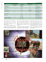
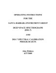
astro imaging
Getting the Most from a
CCD Spectrograph
Amateurs with backyard telescopes are taking their own spectra of stars, nebulae, and galaxies. But there’s more
D
uring the latter half of
the 19th century, amateur
astronomers such as Henry
Draper, Lewis Rutherfurd,
and William and Margaret Huggins took
the lead in developing new spectroscopic
techniques for astronomy that helped establish the emerging field of astrophysics. Dissecting starlight by wavelength
allowed astronomers to determine the
physical nature of the Sun and stars, revealing their chemical compositions, radial velocities, and internal motions.
By Sheila Kannappan and Daniel Fabricant
A century later, high-efficiency CCD
spectrographs allow today’s amateurs to
obtain high-quality spectra from their
backyards, using telescopes no larger than
the ubiquitous 8-inch Schmidt-Cassegrain. Even under light-polluted skies,
such equipment reveals a fascinating variety of features in the spectra of bright
stars. We recently built a fiber-fed CCD
spectrograph for use by students in Harvard University’s astronomy courses. Attached to a 16-inch telescope, it captured
the spectra accompanying this article
from the roof of Harvard’s Science Center, right in the heart of downtown Cambridge, Massachusetts. We use it to observe
bright stars and planets as well as emission lines in deep-sky objects such as the
Orion Nebula and the spiral galaxy M77.
While enterprising amateurs can build
their own spectrographs, both Sivo Scientific (www.sivo.com) and Santa Barbara
Instrument Group (www.sbig.com) offer
commercial units designed for astronomical work. In this article we present some
interesting spectroscopy projects that can
All the spectra with this article were recorded at the
rooftop observatory on Harvard University’s Science Center under some of North America’s most light-polluted
skies. Sheila Kannappan (center) built the observatory’s
spectrograph as a graduate-student project with advice
from coauthor Daniel Fabricant (left) and expert machining assistance from Charles Hughes (right).
S&T: CRAIG MICHAEL UTTER
to it than just recording a spectrum’s image.
Sky & Telescope July 2000
125
®
TELESCOPES
Seeing the real Universe
PRESS RELEASE:
MURNAGHAN Instruments Buys Coulter
Optical® Assets. Production of Odyssey®
Telescopes will continue. New product
benefits from financial stability and
management of MURNAGHAN Instruments Corporation.
®
S&T: CRAIG MICHAEL UTTER
THE ODYSSEY ADVANTAGE
• No assembly required
• Improved Dob mount and focuser
• Double-strength Sonotube
• Eyepiece included
• Many options available
• Lowest prices anywhere
The observatory’s Meade 16-inch telescope
was used for the spectra with this article.
from
8-INCH f/4.5 $39995
• Deep-space scope
• Tube 36 × 10.5 inches
• Diffraction-limited optics
• Includes wide-field eyepiece
• Reengineered mount system
from
8-INCH f/7
$39995
• Lunar/planetary scope
• Tube 56 × 10.5 inches
• Diffraction-limited optics
• Includes high-magnification
eyepiece
• Extra-stable mount
from
10-INCH f/4.5 $54995
• Extremely portable
• Tube 45 × 12.7 inches
• Diffraction-limited optics
• Includes wide-field eyepiece
• Improved mount system
13.1-INCH f/4.5 $89995
• A BIG scope for less money
• Easy 1-person setup
• Tube 57 × 15.7 inches
• Diffraction-limited optics
• Includes wide-field eyepiece
HOW TO ORDER
Send no money. A deposit is NEVER required to
process your order. Pay just before shipment by
check, money order, Visa, or MasterCard.
For orders or information:
Call 1-561-795-2201
Web: www.murni.com
Fax: 1-561-795-9889
ew
The NCoulter
®
Optical
Div. MURNAGHAN Instruments
TM
1781 Primrose Ln.
West Palm Beach, FL 33414
Bigger Scopes . . . Better Optics . . . Less Money
126
July 2000 Sky & Telescope
be done with CCD spectrographs. We also
review the basic concepts of spectroscopy
and the steps involved in obtaining and
calibrating spectroscopic data.
Amateurs are already demonstrating a
remarkable proficiency with CCD spectrographs. One of the most impressive
examples we have seen is Maurice Gavin’s galaxy and quasar redshift measurements (S&T: June 1999, page 14). The
box on page 127 illustrates an easier and
equally entertaining project — observing
the life cycle of stars. We obtained most
of the spectra shown with exposures of
30 seconds or less.
The table on page 128 summarizes the
technical requirements for several spectroscopy projects suited to amateur
equipment. All are within the capabilities
of an 8-inch telescope and a high-quality
spectrograph. Typical projects fall into
two main categories: measuring spectral
properties to determine chemical and
physical processes in celestial objects
and measuring the objects’ radial velocities (speeds along the observer’s line
of sight). The following brief review of
the basic concepts involved can be supplemented with material in books such
as James Kaler’s Stars and Their Spectra
(W. H. Freeman, 1997) and Lawrence
Aller’s Atoms, Stars, and Nebulae (Cambridge University Press, 1991).
Measuring Spectral Properties
Generally speaking, a spectrum consists
of a continuum (light spread over a broad,
continuous range of wavelengths) as well
as some narrow spectral features or lines
superposed on it.
The continuum alone often reveals
something about the conditions under
which the light was produced. In the case
of normal stars, it represents light emitted by the star’s photosphere (visible surface). This light is primarily thermal
blackbody radiation, and thus the wavelength of its peak intensity indicates the
photosphere’s temperature. Hot O and B
stars glow brightest at blue wavelengths,
while our Sun, which is cooler, emits the
most light at yellow and green wavelengths. The coolest, “late-type” stars appear redder.
Many spectra show dark absorption
lines and emission lines, which tell of
other physical processes. The dark lines
arise when molecules and atoms in a
star’s atmosphere absorb continuum light
at specific wavelengths. Late-type stars
show spectra rich in “metal” (heavy-element) absorption lines and sometimes
broad bands of molecular absorption. In
hotter stars molecules are disrupted and
metals are ionized, so most of the absorption lines disappear at visible wavelengths. On the other hand, these “earlytype” stars show the hydrogen Balmer
series of absorption lines prominently.
These hydrogen lines can also appear
as emission features — bright lines in
the spectrum — under different physical
conditions. For example, radiation from
hot O and B stars can ionize surrounding gas clouds and produce line-emitting “H II regions” (astronomer’s shorthand for ionized hydrogen clouds) such
as the Orion Nebula. Hydrogen emission
lines, along with a host of others from elements such as oxygen, nitrogen, and
sulfur, are common in the spectra of
gaseous nebulae.
Measuring Velocities
When a light source is moving along our
line of sight, we can measure its velocity
using the Doppler shift. Just as the pitch
of a train whistle rises and falls as the
train approaches and then recedes, light
waves are blueshifted to higher frequencies when they come from an approaching source and are redshifted to lower
frequencies for a receding source. The
formula for this shift is v/c = ∆λ/λ,
where λ is the wavelength of the spectral
feature for a source at rest, ∆λ is the
change in the wavelength, c is the speed
of light, and v is the velocity of the
source relative to the observer. The ex-
The Life of a Star
Birth. Star-forming regions such as the Orion Nebula glow with the
light of young, hot stars as well as light from the ionized gas bubbles
these stars carve out of the cold gas clouds around them. As the bubbles expand, their shock fronts can compress the rest of the cloud, driving additional waves of star formation. The strong lines in the Orion
Nebula’s spectrum include the hydrogen Balmer series of emission
lines, starting with hydrogen-alpha (656.3 nanometers) and hydrogenbeta (486.1), as well as emission lines of ionized nitrogen (N II at 654.8
and 658.4) and twice-ionized oxygen (O III at 495.9 and 500.7).
Hydrogen-alpha
Doubly ionized
oxygen
500
550
600
650
Wavelength (nanometers)
Midlife. Most stars fall into the familiar OBAFGKM spectral-classifica-
Hydrogen-alpha
B8
Hydrogenbeta
tion system. The earliest types, O and B, represent the hottest, brightest,
and most massive stars, while the later types may be either dwarfs on
the main sequence or giants that have left it. To the eye, early-type stars
like Vega appear pale bluish, while late types like Betelgeuse appear
reddish. An intermediate star such as the Sun (a G dwarf) appears pale
yellow. The reason is clear from the shapes of the continuum spectra
below — the hotter the star, the more energy it emits at shorter, bluer
wavelengths, following the law of blackbody radiation.
Stellar absorption lines also vary by star type. The Balmer series of
lines, including hydrogen-alpha and -beta, are strongest for A stars,
while later-type stars are rich in metal lines such as iron (527.0 nanometers), the sodium D doublet (about 589.5), the magnesium triplet
(about 517.5), and the calcium-iron blend (about 649.5). Although such
metals are also present in early-type stars, at the hotter temperatures
they are more highly ionized, so the neutral metal lines disappear from
the spectrum. In the very latest-type stars, molecular gas forms in the
star’s cool outer atmosphere and causes broad absorption bands such
Stellar Types
Algol
A0
Relative intensity
Ammonia
absorption
band
Jupiter
Planetary Spectra
Saturn
Methane
absorption
band
500
Vega
F2
Relative intensity
Relative intensity
Hydrogenbeta
Old Age and Death. As stars grow old they bloat, oscillate, and explode, leaving tiny remnants made of exotic matter. Massive stars may
die gloriously in supernova explosions, while less massive stars such as
the Sun will form planetary nebulae. Both processes enrich the interstellar gas and provide raw materials for future generations of stars. In our
Harvard program we haven’t yet captured the spectrum of a supernova,
but we have recorded the spectra of planetary nebulae.
Equally spectacular are the
spectra of aging stars such as
the well-known variables
Mira
Mira (Omicron Ceti) and
Gamma Cassiopeiae. Mira is
surrounded by a patchy,
dusty envelope, and its spectrum has a bizarrely sawtoothed structure caused by
500
550
600
650
titanium-oxide
absorption
Wavelength (nanometers)
features. Low-mass stars such
as the Sun are likely to go
Gamma
Hydrogenthrough a similar stage late
beta
Cassiopeiae
in their lives before finally
Hydrogenejecting their envelopes and
alpha
settling down as white
dwarfs. Gamma Cassiopeiae
is orbited by just such a remnant companion — either a
white dwarf or a neutron star.
500
550
600
650
Wavelength (nanometers)
The companion, a bright Xray source, sucks matter from
Gamma Cassiopeiae, and this gas produces Balmer-series emission lines
superposed on the bright star’s B-type stellar spectrum.
Relative intensity
Relative intensity
Orion Nebula
as the titanium-oxide bands at about 590 and 625 nanometers and
other wavelengths.
550
600
650
Wavelength (nanometers)
β Cassiopeiae
G2
Planets. Planets shine by the reflected light of the Sun, but their at-
α Aquarii
Magnesium
K0
Sodium
Iron
Calcium-iron
α Cassiopeiae
K5
Aldebaran
500
550
600
Wavelength (nanometers)
650
mospheres may reprocess that light in interesting ways. Above, the
spectra of Jupiter and Saturn reveal a broad methane-absorption feature at about 620 nanometers superposed on the reflected G-type
solar spectrum. Jupiter’s atmosphere also creates an ammonia-absorption feature from 640 to 650 nanometers. Both spectra are somewhat
redder than the Sun’s because the planets’ atmospheres preferentially
reflect red light.
Sky & Telescope July 2000
127
astro imaging
Spectroscopy-Project Ideas
Project
Stellar spectral types
Solar-system objects
Variable stars
Supernova identification
Required resolution
(nanometers)
1
1
Spectral range
(nanometers)
470–670
470–670
Magnitude range
0–5
0–10
1
1
470–670
350–700
Stellar radial velocities
0.3
470–670
3–15
Limited only by
your ambition
0–5
Nebular emission lines
1+
470–670
14+
Galaxy redshifts
1+
650–700
(for example)
470–780
(or any subrange)
14+
Emission lines in active galactic
nuclei (AGNs) including quasars
0.3–1+
pansion of the universe also produces a
cosmic redshift, defined as z = ∆λ/λ. Cosmic redshifts are often converted into
units of velocity according to v = cz for
small values of z.
In addition to displacing the wavelengths of spectral lines, Doppler shifts
can also broaden the lines if material is
moving at a range of different velocities.
T
14+
Some of the broadest lines result from
material swirling around and falling into
black holes at the centers of galaxies. In
such cases a velocity spread of about
1,000 kilometers per second is often
observed.
The ability to measure line broadening
is directly limited by the wavelength resolution of a spectrograph, which can be
he first total solar eclipse of the new millennium occurs on June 21, 2001, in exotic
southern Africa. Sky & Telescope and
Scientific Expeditions will be there,
and we invite you to join us! We’ll
rendezvous with the Moon’s shadow
in Zambia, where weather prospects
are excellent and totality lasts nearly 4
minutes. We’ll also go on safari in South
Africa’s best game reserves, visit majestic
Victoria Falls, and view the spectacular
southern sky with the Milky Way high
overhead and the Magellanic
Clouds near the meridian.
Our 11-day expeditions
begin June 15th. Prices
start at $5,325 per
person, based on
double occupancy.
Space is limited —
make your reservation today!
Scientific Expeditions, Inc.
For more information
227 West Miami Ave., Suite #3
call toll free
Venice, FL 34285
800-344-6867
Fax: 941-485-0647
®
or point your Web browser to http://www.skypub.com/
E-mail: [email protected]
store/scienx/africa2001.html
128
July 2000 Sky & Telescope
Notes
350–900 better
350–900 better. Outer
planets hard to track
350–900 better
0.5-nanometer resolution
better. Smaller range okay
Requires careful
wavelength calibration
Lower resolution a help for
faint targets
Choose range based on
redshift and desired lines
Choose subrange based on
redshift and desired lines
converted into velocity units using the
Doppler shift formula given above, where
∆λ is the wavelength resolution, λ is the
central wavelength being observed, and
the velocity resolution v is the result of
the calculation. However, one can often
measure overall redshifts and blueshifts
with a precision much better than the
resolution limit.
African
ECLIPSE
Safari
CCD counts
Calibrating a
Spectrum
0
100
550
600
200
650
200
300
Wavelength
Calibrated
300
Pixel Number
Optical Astronomy Observatory (http://
iraf.noao.edu/iraf/web/). Unfortunately,
IRAF has a steep learning curve and
runs only on Unix or Linux operating
systems. Another powerful analysis program is Research Systems’s IDL (www.
rsinc.com). Although quite expensive, it
is user friendly and will run on any
computer platform. Free astronomy tools
for IDL are available on the Web (http://
idlastro.gsfc.nasa.gov/homepage.html).
WaveMetrics’ IGOR (www.wavemetrics.
com) is much less expensive than IDL,
and it offers extensive built-in graphing
and analysis features as well as programming capabilities. IGOR was not designed specifically for astronomy, but it
is flexible and the user’s manual and
technical support are excellent.
Some other programs that may be useful include Maxim DL (www.cyanogen.
com), PDL (the Perl Data Language,
available free from http://www.aao.gov.
au/local/www/kgb/pdl/), and DS9 (a
quick-look program we use to check exposure levels of the data obtained at the
telescope, available free from http://heawww.harvard.edu/RD/ds9/). DS9 lets you
500
550
600
650
Wavelength (nanometers)
Relative intensity
Transforming images from a CCD spectrograph into useful spectra requires a series of calibration steps. The authors’ fiber-fed spectrograph produces a discrete spectrum for each of
its six fibers. At top is the featureless-looking spectrum image for the star Algol, the light of
which fell on a single fiber. Plotting the brightness of rows of pixels spanning this spectrum produces the raw-data graph. Another spectrum image of light from a mercury-neon
calibration lamp (illuminating all six fibers) and its corresponding plot determines the
wavelength recorded by each pixel in the row and is used to wavelength calibrate the astronomical spectrum. This spectrum, however, is still highly distorted because of instrumental effects, in particular the varying spectral sensitivity of the CCD detector. Only when
flux calibrated (see page 130) does the plot accurately reveal Algol’s spectral features.
Hardware and Software
In addition to a spectrograph and telescope, a handy piece of auxiliary equipment is a calibration lamp. An ideal
lamp has many narrow emission lines
throughout the wavelength range of interest. These lines are useful for focusing
the spectrograph and determining wavelengths within a spectrum. With our student spectrograph we use a mercury-neon
lamp sold by Oriel Instruments (150
Long Beach Blvd., Stratford, CT 06615;
www.oriel.com).
Spectral-analysis software is not as mature as the image-processing programs
widely available to today’s amateur astronomers. Nevertheless, you will need
analysis software to perform essential
calibration of your CCD spectra, without
which the spectra will appear distorted
and difficult to interpret. Commercial
units such as the SBIG spectrograph usually come with basic software, but you
may need to supplement it.
Professional astronomers often process their spectral data using IRAF, the
free image-processing and data-analysis
software available from the National
100
Pixel Number
CCD counts
Wavelength (nanometers)
500
Extracted Spectrum
After Bias Subtraction
0
Neon (650.65)
Neon (614.31)
Mercury (546.07)
CCD counts
Mercury (491.80)
Mercury-Neon
Calibration
Lamp
Raw Data
Flux Calibrated
500
550
600
650
Wavelength (nanometers)
run a mouse over a CCD image and instantly obtain an intensity plot for the
row of pixels under the cursor.
Exposure Times
Spectroscopy in general, and high-resolution spectroscopy in particular, requires longer exposure times than conventional imaging. This is because light
from a star or other source is spread into
a spectrum that covers many pixels on
the CCD rather than being concentrated
onto just a few as in direct imaging. The
more widely the light is spread out into
a spectrum, the more sharply we can resolve closely spaced spectral features. But
this higher resolution comes at the expense of diluting the light and thus requires longer exposures. Many other factors also affect exposure time —
telescope aperture, spectrograph efficiency, noise characteristics of the CCD camera, and sky brightness, to name a few.
Rather than modeling all these factors,
we have found the easiest way to make
exposure calculations is by scaling from
other spectroscopic observations of similar objects. Once you have obtained sucSky & Telescope July 2000
129
astro imaging
cessful spectra for a few objects, simply
multiply those exposures by a factor of
2.5 for each magnitude fainter that you
wish to observe. This technique works
only for stars, since typically just a small
fraction of the light from extended objects passes through a spectrograph slit.
On the other hand, an emission nebula is
sometimes much easier to observe with a
spectrograph than its surface brightness
would imply, since almost all of its light
will be concentrated in a few bright emission lines rather than spread across a continuum.
With our 16-inch telescope and the
spectrograph operating at 0.6-nanometer
resolution, we obtain the spectrum of a
2nd-magnitude star with a 10-second exposure. Switching to 1.6-nanometer resolution, we can get a spectrum of the
Ring Nebula or the galaxy M77 by combining a pair of 5-to-10-minute exposures. Since the characteristics of most
amateur spectrographs will be roughly
comparable to ours, these exposure times
will approximately scale by telescope
aperture for point sources. For example,
an 8-inch telescope has one-quarter the
light-collecting area of our 16-inch, so it
would need a 40-second exposure for a
2nd-magnitude star. For extended
sources, the exposure time will also depend on what fraction of the object is
imaged onto the spectrograph’s entrance
aperture — decreasing a telescope’s focal
length or increasing the entrance aperture will decrease the exposure time. Just
as with conventional CCD imaging, exposures longer than about 10 minutes
should be “assembled” from a series of
shorter exposures to make it easy to remove things like cosmic-ray artifacts
from the final image.
Calibration
Unlike a raw pictorial image, a raw spectrograph image does not always resemble
the final calibrated data that will be extracted from it. Without calibration, the
raw frame yields a spectrum that is highly distorted by the way the telescope and
spectrograph transmit and detect different wavelengths of light. Fortunately,
most of this distortion can be removed
with a basic calibration procedure that
corrects for everything except atmospheric absorption. We applied this sort
of minimal processing to calibrate the
spectra with this article. The data reduction consists of three essential parts:
background subtraction, wavelength
calibration, and flux calibration.
Background subtraction removes unwanted signal in the spectra due to the
CCD’s bias and dark current as well as
light pollution from the sky. A simple
way to accomplish this is to take an
identical exposure of the blank sky next
to the object and subtract it from the
spectrum image. Unfortunately, this
method wastes precious observing time,
so we usually use a different procedure.
Since bias subtraction is a necessary
step for any further calibration, we remove the bias and the dark current simultaneously by subtracting the average
pixel value obtained from pixels on the
CCD adjacent to those recording the
spectrum. While this method is not perfect (using an average value does not
take into account unusually “hot” or
Flux Calibrating CCD Spectra
T
he table on page 131 lists some bright
stars for which reference spectra, sampled every 1.6 nanometers (16 angstroms) between 330 and 755 nanometers,
are available on the Web (http://adc.gsfc.
nasa.gov/adc-cgi/cat.pl?/catalogs/2/2179/).
The fluxes in the reference spectra are given
in monochromatic magnitudes, which may
be converted to absolute flux at any given
wavelength using the equation
For example, the reference star HR 8634 has
a monochromatic magnitude of +3.4 at a
wavelength of 555.6 nanometers. Evaluating
the above equation gives an absolute flux of
about 430 photons per square centimeter per
second per nanometer at this wavelength.
Because a CCD’s pixel value is directly proportional to the number of photons striking
it (as long as the pixel value remains well
below its saturation level) you can perform a
first-order flux calibration by dividing your
observed spectrum of a standard star into
the star’s reference spectrum obtained from
the Web site. (Before dividing, you may need
to manipulate the reference spectrum to
match the range and resolution of the ob-
F λ = 5.5 × 106 (1/λ) 10 –0.4(mag),
where Fλ is given in photons per square centimeter per second per nanometer, λ is the
wavelength in nanometers, and mag is the
monochromatic magnitude.
served spectrum.) The result will be a ratio of
the star’s “official” spectrum to the spectrum
your equipment recorded at the various
wavelengths.
It is now a simple matter to multiply all
your spectra by this correction. Doing this removes all flux distortions introduced by your
equipment. If you don’t care about the details of atmospheric absorption or about getting absolute flux levels, then this procedure
is all you need. In fact, the spectra accompanying this article were reduced by this
method. Furthermore, you can reuse the
same standard-star data over and over if your
setup doesn’t change. We use one calibration
for many nights.
Saturn
calibrated
uncalibrated
500
550
600
Wavelength (nanometers)
130
Relative intensity
Relative intensity
Methane
absorption
band
July 2000 Sky & Telescope
650
Algol
calibrated
uncalibrated
500
550
600
Wavelength (nanometers)
650
“cold” pixels), it is adequate for brightstar work, where there is a lot of signal
relative to the level of the bias and dark
current.
For fainter targets it is important to
subtract the sky background as well as
the pixel-by-pixel bias and dark current,
because an errant pixel or emission from
skyglow could easily be mistaken for a
real feature in a weak spectrum. With a
slit-type spectrograph, the sky is present
across the whole slit, so its level can be
estimated from pixels adjacent to the target’s spectrum. Our spectrograph uses
optical fibers to transfer light from the
telescope to the spectrograph, where the
fibers are arranged in a line to act like an
entrance slit. With this system a fiber at
the telescope’s focal plane can be positioned on blank sky to record the background while a matching fiber is positioned on the target. To remove the sky
background, we wavelength-calibrate the
sky’s spectrum as described below and
subtract it from the target’s wavelengthcalibrated spectrum.
With very long exposures, cosmic-ray
artifacts become a problem. In this case,
multiple exposures should be taken and
ZIP OUT ROOF
Bright Standard Stars
Star
29 Piscium
ξ2 Ceti
π2 Orionis
η Hydrae
θ Crateris
θ Virginis
108 Virginis
58 Aquili
ε Aquarii
ζ Pegasi
Designation
HR 9087
HR 718
HR 1544
HR 3454
HR 4468
HR 4963
HR 5501
HR 7596
HR 7950
HR 8634
R.A. (2000.0) Dec.
00h 01m 50s
–03 01.7
02h 28m 10s
+08 27.6
04h 50m 37s
+08 54.0
08h 43m 14s
+03 23.9
11h 36m 41s
–09 48.1
13h 09m 57s
–05 32.3
+00 43.0
14h 45m 30s
+00 16.4
19h 54m 45s
20h 47m 41s
–09 29.8
22h 41m 28s
+10 49.9
any artifacts identified in a search for
small bright spots that appear in one
image but not the others. These can be
removed when the spectra are added together.
The goal of wavelength calibration is
to determine the wavelength at each
pixel in the spectrum. Fortunately, a
spectrograph that uses a diffraction grating to disperse light has, to a first approximation, a linear relationship between wavelength and pixel position.
Thus, a few recognizable emission or absorption lines in the image will provide
enough information to determine the
AFTER
BEFORE
EASY SETUP
DURABLE
PORTABLE
RAINFLY
$390.00
ROOMY
ETX............$30.00
C5..ETX 125....$30.00
AP 105mm..$30.00
AP 130mm..$30.00
AP 155mm..$35.00
7” Mak........$40.00
8” SCT........$40.00
9.25” SCT.....$45.00
10”
11”
12”
14”
SCT........$45.00
SCT........$50.00
SCT........$55.00
SCT........$60.00
Magnitude
5.1
4.3
4.4
4.3
4.7
4.4
5.7
5.6
3.8
3.4
Spectral type
B7 III–IV
B9 III
A1 V
B3 V
B9.5 V
A1 I
B9.5 V
A0 III
A1 V
B8 V
entire wavelength scale. The simplest solution is to observe an astronomical
source with strong and easily identifiable
lines, such as the Orion Nebula or Gamma Cassiopeiae. In this case you may
wish to compensate for any Doppler shift
in the reference spectra due to the object’s radial velocity. A more accurate
wavelength calibration requires the spectrum of a calibration lamp.
The stability of this wavelength calibration throughout the night depends
on whether the spectrograph optics flex
as the telescope moves or the temperature changes. With our fiber-fed, bench-
controller..............$70.00
.965”.....................$33.00
1.25”.....................$35.00
2”.........................$38.00
3”.........................$40.00
4”.........................$43.00
5”.........................$45.00
6”..........................$48.00
7/8”......................$50.00
9/10”..................$60.00
11”.....................$65.00
12”.......................$70.00
14/16”..................$80.00
Telrad heater..............$23.00
Telescope computer control
heater ...........................$35.00
Felt lined Flexible Dewcaps
ETX.....................................$25.00
C5 / ETX 125....................$32.00
6”..........................................$42.00
7”/C8”..................................$50.00
C9.25...................................$55.00
10”........................................$60.00
C11”.....................................$70.00
12”........................................$85.00
C14”..................................$105.00
4 ZIP OUT SLOTS
LIGHTPROOF
FAST SETUP
PORTABLE
DURABLE
ROOMY
$375.00
ULTIMATE......$125.00
Optional rain fly
$95.00
ULTIMATE II...$160.00
Ultimate II has a
folding accessory
tray for eyepieces
filters, charts etc.
Made from Baltic
Birch Plywood.
Seat is adjustable
from 9” to32”
Buy Direct or from your favourite dealer
Collimators for
Schmidt Cassegraines
and Newtonians
1.25” ....$100.00
2” .........$110.00
SCT.......$160.00
SCT-NGF-s....$175.00 ........
Flexible, Felt lined, Durable.
Save up to 85% vs Brand Name.
12V 17 AMP HOUR
Comes with float charger, carry bag, built in
fused cigarette lighter power socket. ....$125.00
33 AMP HOUR BATTERY
Face of collimator angled at 45° for easy reading.
4 fused power plugs, LCD for state of charge,
1 amp float charger, carry bag
Comes in two configurations
We are the exclusive North American distributors for
Coronado Instruments H-Alpha filters and telescopes.
Dealer inquiries welcome.
12 volt......$290.00
18 volt......$390.00
ASP 60..............$2625.00
ASP 60/BF30....$3125.00
AS1 90..............$7200.00
Helios 1............$2925.00
18 volt version is for LX 200 owners.
One plug has a built in inverter for 18 volt
output.
We accept all major credit cards
KENDRICK ASTRO INSTRUMENTS
2920 Dundas St. West, Toronto, Ont M6P 1Y8, Canada
Tel 416 762 7946 Fax 416 762 2765
kendrick-ai.com
email: [email protected]
Sky & Telescope July 2000
131
mounted spectrograph, we can use a single wavelength calibration for an entire
night and indeed for weeks.
Flux calibration involves observing a
standard star, dividing its spectrum as
recorded by the spectrograph by its “official” spectrum as determined from a reference database, and using the result to
correct the flux levels of the rest of your
data (see the box on page 130).
Because there are only a few bright
standard stars, there will not always be
one conveniently placed for calibration.
As an alternative, if you don’t need an accurate flux calibration but just want to
remove gross instrumental distortions,
you may prefer to record the spectrum of
a bright star with the same spectral type
and luminosity class as one of the standard stars, and then compare the spectra.
(Stellar classification information is available on the Web at http://simbad.harvard.
edu.) This strategy has the advantage of
giving you a wider choice of calibration
stars at the expense of introducing small
errors due to differences in spectral shape
and radial velocity.
A remaining concern is atmospheric
absorption, which takes its heaviest toll
at the blue end of the spectrum. The
basic flux calibration described above
partially corrects for this effect. However,
a more thorough calibration is needed to
refine the correction. Absorption by the
Earth’s atmosphere depends on how high
the object is in the sky. At low altitudes
the light path through the atmosphere is
long and results in greater absorption. To
model this effect requires observing standard stars at different altitudes. Alternatively, you can skip the modeling if you
observe a standard star very close to the
object of interest immediately before or
after recording the object’s spectrum, so
that the light path through the atmosphere is similar for both targets. This
method is preferable if there are thin
clouds present.
Have Fun!
This article gives an overview of the tools
and techniques you need to collect, work
with, and understand spectra. Amateur
spectroscopy is entering a renaissance,
and the fun is just beginning!
Sheila Kannappan and Daniel Fabricant
are astronomers at the Harvard-Smithsonian
Center for Astrophysics, with special interests
in the evolution of galaxies and the large-scale
structure of the universe.
132
July 2000 Sky & Telescope
Win ...
JMI’s
a $1,000 NGT-6
telescope!
PAT
PENDING
1-1/4” anodized with
stainless steel bearings:
LIGHTWEIGHT
LOWCOST
HIGHQUALITY
ANSWER
to PLASTIC
FOCUSERS!
$79 ($7 S&H)
2” anodized with
stainless steel bearings:
$99 ($7 S&H)
NAME THIS FOCUSER and you
could win this NGT-6 telescope!
JMI’s revolutionary low profile,
zero image shift, solid aluminum,
reverse Crayford focuser is so
ASTOUNDING it has left us
SPEECHLESS, so we’re asking
YOU to help us name it!
New!
NGF-SE FOCUSER
SCHMIDT-CASSEGRAIN Manual version of JMI’s
famous zero-image-shift
FOCUSER
NGF-S focuser. Fits Meade and
•
NGF-SE Focuser
$169
($7 S&H)
•
•
•
•
•
Celestron Schmidt-Cassegrain
telescopes (SCT). Features:
Extra fine control, one rotation
of the knob gives 0.39” travel.
Low profile adds less than 2-1/2”.
Heavy duty, carries 8 pounds.
Solid anodized aluminum.
Focus lock.
2” output plus threaded output
adapter. All SCT accessories
can be used.
CONTEST RULES:
Send us your name suggestion for this revolutionary focuser, and if we choose your product name you will receive
FREE an NGT-6 telescope (a $1,000 value—you only pay for the shipping). Names should be short; acronyms are
fine. Send more than one if you wish, but no more than five. Entries must be sent by mail (pls. no e-mail). In case of
duplicates, the earliest post mark will qualify. Must be postmarked by 7/31/00. JMI’s employees and families not
eligible. Winner notified by 9/1/00. Suggested names not allowed: JMI Focuser, Reverse Crayford, Jim Burr Focuser.
Offer void where prohibited.
Jim’s Mobile Inc. • 810 Quail St. Unit E • Lakewood, CO 80215
Orders: 800-247-0304 • Info: 303-233-5353 • Fax 303-233-5359