Download CREPT-MCNP 1.1

JAEA-Data/Code
CREPT-MCNP 1.1 (Calibration Code for the Representative
Point Method with MCNP) : User Manual -Version 1.1.0
Jun SAEGUSA
Department of Radiation Protection
Nuclear Science Research Institute
Tokai Research and Development Center
October 2008
Japan Atomic Energy Agency
日本原子力研究開発機構
JAEA-Data/Code
2008-017
JAEA-Data/Code
2008-017
JAEA-Data/Code
2008-017
CREPT-MCNP 1.1 (Calibration Code for the Representative Point Method with MCNP)
: User Manual -Version 1.1.0
Jun SAEGUSA
Department of Radiation Protection
Nuclear Science Research Institute
Tokai Research and Development Center
Japan Atomic Energy Agency
Tokai-mura, Naka-gun, Ibaraki-ken
(Received July 7, 2008)
The representative point method is a novel method which enables efficiency calibrations using a
standard point source. A calculation code for use in implementation of the method has been developed. The
code is named CREPT-MCNP (Calibration Code for the Representative Point Method with MCNP).
The code estimates the position of a representative point which is intrinsic to each volume sample shape,
and also provides self-absorption factors that correct the efficiencies measured at the representative point with
a standard point source. It can deal with photons between 20 keV and 2 MeV with p- or n-type germanium
semiconductor detectors. CREPT-MCNP runs in the Windows PC environment as a GUI based application.
This manual describes the features of the CREPT-MCNP code.
Keywords: CREPT-MCNP, Efficiency Calibration, Representative Point Method, Standard Source,
Traceability, Radioactivity Measurement, Gamma-ray, Self-absorption, Efficiency Curve
i
JAEA-Data/Code
2008-017
JAEA-Data/Code
2008-017
CREPT-MCNP 1.1
㸦௦⾲Ⅼἲࢆ⏝࠸ࡓࢤ࣐ࣝࢽ࣒༙࢘ᑟయ᳨ฟჾࡢຠ⋡ᰯṇ⏝ࢥ࣮ࢻ㸧
࣮ࣘࢨ࣮࣐ࢽࣗ࢔ࣝ 1.1.0 ∧
᪥ᮏཎᏊຊ◊✲㛤Ⓨᶵᵓ ᮾᾏ◊✲㛤Ⓨࢭࣥࢱ࣮
ཎᏊຊ⛉Ꮫ◊✲ᡤ ᨺᑕ⥺⟶⌮㒊
୕ᯞ ⣧
㸦2008 ᖺ 7 ᭶ 7 ᪥ཷ⌮㸧
௦⾲Ⅼἲࡣࠊᶆ‽Ⅼ≧⥺※ࢆ⏝࠸࡚ࢤ࣐ࣝࢽ࣒༙࢘ᑟయ᳨ฟჾࡢຠ⋡ᰯṇࢆ⢭ᗘࡼࡃ⾜࠺ࡓࡵ
ࡢ᪉ἲ࡛࠶ࡿࠋ௦⾲Ⅼἲࢆ෇⁥࡟ᐇ᪋ࡍࡿࡓࡵࡢィ⟬ࢥ࣮ࢻ࡜ࡋ࡚ࠊ௒ᅇࠊCREPT-MCNP 1.1
㸦Calibration Code for the Representative Point Method with MCNP㸧ࢆᩚഛࡋࡓࠋ
ࡇࡢィ⟬ࢥ࣮ࢻ࡟ࡣࠊయ✚ヨᩱࡢィᩘຠ⋡᭤⥺࡟➼౯࡞ィᩘຠ⋡᭤⥺ࢆ୚࠼ࡿⅬ㸦௦⾲Ⅼ㸧ࢆ
᥈⣴ࡍࡿࡓࡵࡢᶵ⬟ࡸࠊ௦⾲Ⅼ࡛ ᐃࡋࡓィᩘຠ⋡࡟ᑐࡋ⮬ᕫ྾཰ຠᯝࡢ⿵ṇࢆ⾜࠺ᶵ⬟࡞࡝ࡀ
ྵࡲࢀ࡚࠾ࡾࠊࡇࢀࡽࡢᶵ⬟ࢆᐇ⾜ࡍࡿࡇ࡜࡟ࡼࡾ┠ⓗ࡜ࡍࡿィᩘຠ⋡ࢆᚓࡿࠋホ౯ᑐ㇟ࡣࠊp
ᆺ࠾ࡼࡧ n ᆺ Ge ༙ᑟయ᳨ฟჾ࡟ࡼࡾ ᐃྍ⬟࡞ࠊ࢚ࢿࣝࢠ࣮⠊ᅖࡀ 20 keV ࠿ࡽ 2 MeV ࡢගᏊ
࡛࠶ࡿࠋCREPT-MCNP1.1 ࡣࠊWindows PC ⎔ቃ࡛ GUI ᙧᘧ࡛ືసࡍࡿࠋᮏሗࡣࠊCREPT-MCNP
ࡢᶵ⬟࡜౑⏝᪉ἲ࡟ࡘ࠸࡚࡜ࡾࡲ࡜ࡵࡓࡶࡢ࡛࠶ࡿࠋ
ཎᏊຊ⛉Ꮫ◊✲ᡤ㸸ࠛ319-1195 Ⲉᇛ┴㑣⌃㒆ᮾᾏᮧⓑ᪉ⓑ᰿ 2-4
ii
ii
JAEA-Data/Code　2008-017
Contents
1 Introduction ············································································································
1
2 CREPT-MCNP Code User Manual ······································································
2
2.1 System Requirements ······································································································
2
2.2 Installation ·······················································································································
2
2.3 Directory Configuration ···································································································
5
2.4 Basic Operation ···············································································································
6
2.5 Operation Menus ·············································································································
8
2.5.1 [File] Menu ···············································································································
8
2.5.2 [Data] Menu ··············································································································
9
2.5.3 [Calculation] Menu ··································································································· 35
2.5.4 [Calculation Results] Menu ······················································································· 45
3 Efficiency Calibration of Radioactivity Measuring Instrument with the
Representative Point Method ·············································································· 53
3.1 Present Status of Efficiency Calibration ·········································································· 53
3.2 Efficiency Calibration with the Representative Point Method ········································· 54
3.3 Utilisation of CREPT-MCNP Code ················································································· 56
3.3.1 Calculation time needed for efficiency calibration ···················································· 56
3.3.2 Uncertainty estimation ······························································································ 57
3.4 Application of the Method ······························································································· 57
4 Summary and Perspective for the Future ··························································· 58
Acknowledgements ······································································································
References ·····················································································································
Appendices Format Description of Input and Output data ································
A.1 Output File for the Efficiency-Curves Group A ····························································
58
59
60
60
A.2 Output File for the Efficiency-Curves Group B ······························································ 61
A.3 Output File for Position of the Representative Point and Parameter t ····························· 62
A.4 Output File for the Efficiency Curves Used
for Self-Absorption Correction ······················································································ 65
A.5 Output File for the Final Efficiency Curve ······································································ 66
A.6 Input File for Measured Efficiency Curve at the Representative Point ··························· 67
A.7 Input File for Angular Dependence of Efficiencies ························································ 68
A.8 Description of Basic Element ························································································· 69
iii
iii
JAEA-Data/Code　2008-017
┠ ḟ
㸯 ࡣࡌࡵ࡟ ···································································································································
1
㸰 CREPT-MCNP ࢥ࣮ࢻ࣮ࣘࢨ࣮࣐ࢽࣗ࢔ࣝ ·····································································
2
2.1 ࢩࢫࢸ࣒ᵓᡂ ···············································································································
2
2.2 ࢖ࣥࢫࢺ࣮ࣝ ···············································································································
2
2.3 ࢹ࢕ࣞࢡࢺࣜᵓᡂ ······································································································
5
2.4 ᇶᮏ᧯స ·······················································································································
6
2.5 ࣓ࢽ࣮ࣗ᧯స ···············································································································
8
2.5.1 [ࣇ࢓࢖ࣝ]࣓ࢽ࣮ࣗ ·····························································································
8
2.5.2 [ࢹ࣮ࢱ]࣓ࢽ࣮ࣗ ·································································································
9
2.5.3 [ィ⟬]࣓ࢽ࣮ࣗ ·····································································································
35
2.5.4 [ィ⟬⤖ᯝ]࣓ࢽ࣮ࣗ ·····························································································
45
㸱 ௦⾲Ⅼἲࢆ⏝࠸ࡓᨺᑕ⬟ ᐃჾࡢຠ⋡ᰯṇ ····································································
53
3.1 ຠ⋡ᰯṇࡢ⌧≧ ··········································································································
53
3.2 ௦⾲Ⅼἲ࡟ࡼࡿຠ⋡ᰯṇ ··························································································
54
3.3 CREPT-MCNP ࢥ࣮ࢻࡢ฼⏝ ····················································································
56
3.3.1 ຠ⋡ᰯṇ࡟せࡍࡿ᫬㛫 ·······················································································
56
3.3.2 ୙☜࠿ࡉࡢホ౯ ···································································································
57
3.4 ௦⾲Ⅼἲࡢ฼⏝ ··········································································································
57
㸲 ࡲ࡜ࡵ࡜௒ᚋࡢᒎᮃ ··············································································································
58
ㅰ㎡ ····················································································································································
58
ཧ⪃ᩥ⊩ ············································································································································
59
௜㘓 ධฟຊࣇ࢓࢖ࣝࡢᵓᡂ ······································································································
60
A.1 ィᩘຠ⋡᭤⥺⩌ A ࡢィ⟬⤖ᯝࣇ࢓࢖ࣝ ································································
60
A.2 ィᩘຠ⋡᭤⥺⩌ B ࡢィ⟬⤖ᯝࣇ࢓࢖ࣝ ································································
61
A.3 ௦⾲Ⅼ఩⨨࠾ࡼࡧᣦᶆ t ࡢィ⟬⤖ᯝࣇ࢓࢖ࣝ ······················································
62
A.4 ⮬ᕫ྾཰⿵ṇಀᩘィ⟬⏝ࡢຠ⋡᭤⥺ィ⟬⤖ᯝࣇ࢓࢖ࣝ ····································
65
A.5 ᭱⤊ຠ⋡᭤⥺ࣇ࢓࢖ࣝ ·····························································································
66
A.6 ௦⾲Ⅼ࡛ࡢᐇ ࢹ࣮ࢱධຊࣇ࢓࢖ࣝ ·····································································
67
A.7 ィᩘຠ⋡ࡢゅᗘ౫Ꮡᛶࢹ࣮ࢱධຊࣇ࢓࢖ࣝ ·························································
68
A.8 ᇶᮏࣃ࣮ࢶ ··················································································································
69
iv
iv
JAEA-Data/Code　2008-017
Disclaimer & Intellectual Property Statement
CREPT-MCNP is a calculation code for use in carrying out efficiency calibrations with the
representative point method. The code can be found in the PRODAS database administered by the
Center for Computational Science & e-Systems, Japan Atomic Energy Agency. Users must obtain
the code through the center and use it in compliance with the administrative computer program rules
set by the center.
The CREPT-MCNP code is provided free of charge to the academic research community or
public organisations for non-commercial, non-profit internal research use. Prior to use of the code,
users will need to individually obtain and install the MCNP code as it is not included with the
CREPT-MCNP code. Note that neither the author or any Japan Atomic Energy Agency member
can be held responsible for results obtained using the code and/or that the representative point
method will meet the users’ requirements, nor any damage or loss resulting from its use.
A request for the representative point method is to be examined for a Japanese patent by the
Japan Patent Office and has been made with an Application Kokai Publication Number of 200298768.
v
This is a blank page
JAEA-Data/Code　2008-017
1 Introduction
One of the most important tasks with the radiation control work is precisely and promptly measuring
radioactivity in environmental samples. And in addition, with the rapid widespread use of accelerators these
days, the urgent need to be able to estimate the induced radioactivity in activated samples of various shapes
and materials has arisen. Radioactivity measurements for these purposes are generally based on gamma-ray
spectrometry using HPGe detectors. In order to quantify the radioactivity, an efficiency calibration, viz.
determination of the peak-efficiency curves versus energy, must be achieved for various combinations of
sample-detector geometries. The shape and magnitude of the peak-efficiency curve depends on the detector,
sample shape and sample material.
Generally, efficiency calibrations are performed by manufacturing a standard volume source spiked
with a known amount of radioactivity and then measuring it with the detector. Manufacturing standard volume
sources, however, requires skilful and complicated techniques [Sa95], and the procedure must be repeated
periodically as they contain rather short-lived nuclides. Furthermore, differing standard volume sources must
be prepared depending on the individual sample’s shape and material, which can result in an undesirable
increase in radioactive waste as one has to get rid of them. Although peak-efficiency curves can be determined
using only computational approaches, the reliability of the results cannot be ensured, mainly due to difficulties
in modelling the detector, on particular with parameters such as the dead layer or the ineffective region of the
germanium crystal [Jo06] [He03].
To overcome this problem, the representative point method, a novel method which enables efficiency
calibrations using a standard point source, has been previously proposed [Sa00] [Sa04], and a calculation code
for implementing the method newly developed [Sa08]. The code is named CREPT-MCNP (Calibration Code
for the Representative Point Method with MCNP).
The code finds the position of the representative point, the position where a point source efficiency
curve better approximates that one for the volume source. Self-absorption correction factors are also computed
to make correction on the efficiencies measured at the representative point with a standard point source. It
involves the general-purpose Monte Carlo code MCNP [Br00] [XM05] for simulating radiation transport in
and around the sample and detector. The developed CREPT-MCNP code has MCNP control functions, e.g.,
creation of input files and simulation with MCNP, as a GUI (Graphical User Interface) based application.
Even novice MCNP users can carry out efficiency calibrations through use of this code.
−　−
1
JAEA-Data/Code　2008-017
2 CREPT-MCNP Code User Manual
2.1 System Requirements
The CREPT-MCNP code is packaged software for readily implementing efficiency calibrations. It was
developed using Microsoft Visual Basic.NET, Lahey Fortran 95, and SPREAD for .NET Windows Forms
Edition (version 1.0.9.0).
The code works under Microsoft Windows® operating systems version 2000 or XP, and allows users
easy and interactive operation with a GUI. The recommended amount of PC RAM memory is at least 256
megabytes.
Either MCNP code version 4 [Br00] or 5 [XM05] and their associated cross-section library data are
necessary and should be located in a selected directory within the system. When version 5 MCNP is used, the
X-windows system need to be run in order to make the geometric models draw on the display. The Xwindows system can be freely established on Windows PCs using the Cygwin tool [CY08], which is available
via the internet. The geometry plotting itself is done with a built-in function, originally included in MCNP as
the “-ip” protocol.
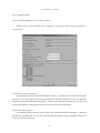
2.2 Installation
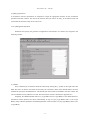
CREPT-MCNP can be installed according to the following steps (1) to (5).
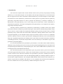
(1) Double-click the “Setup.msi” icon on the installation CD. If .NET Framework has not been installed on the
PC, the following message appears. In the case, users should install it by clicking [Yes], which then directs
users to the Microsoft .NET Framework website. If installation was successful, go to the step (3),
otherwise, step (2).
(2) Double-click the “dotnetfix.exe” icon on the installation CD to install .NET Framework 1.1. Note that the
“dotnetfix.exe” file on the CD is not the latest version.
−　−
2
JAEA-Data/Code　2008-017
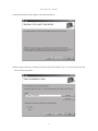
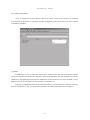
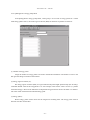
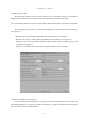
(3) When the following window appears, click the [Next] button.
(4) Select a folder (directory) in which to install the code. Select whether a user or users can run the code, and
then click the [Next] button.
−　−
3
JAEA-Data/Code　2008-017
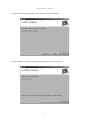
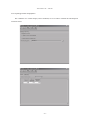
(5) When the following window appears click [Next] to commence installation.
(6) Once installation is complete, the following window appears. Click [Close] to exit.
−　−
4
JAEA-Data/Code　2008-017
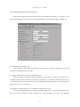
2.3 Directory Configuration
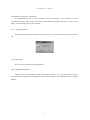
Execution of the code will automatically create the subdirectory structure shown in Fig. 2-1 within the
directory designated in step (4) of the previous section.
crept
Stores main program, .dll files and help files
system
Stores data required for system execution
lib
Stores dummy libraries used in chkregion.exe
parts
Stores data of default parts (stylised detectors, samples, etc.)
detector
Stores data of default “detectors”
cover
Stores data of default “covers”
tray
Stores data of default “trays”
jig
Stores data of default “support jigs”
object
Stores data of default “measured samples”
space
Stores data of default “calculation areas”
work
Stores data created by the system, and calculation results
angle
Stores data of angulat dependency (not used in this version of the code)
ExportExcel
Stores data used for post-processing with the Microsoft Excel
effA
Stores data of efficiency-curves group A
effB
Stores data of efficiency-curves group B
effC
Stores data of “representative point (RP)” and “parameter t”
material
Stores data of material compositions and densities
meas
Stores measured efficiency data at RP with a standard point source
model
Stores geometrical model data for MCNP calculations
parts
Stores data of parts (user-established data)
detector
Stores data of “detectors”
cover
Stores data of “covers”
tray
Stores data of “trays”
jig
Stores data of “support jigs”
object
Stores data of “measured samples”
space
Stores data of “calculation areas”
selfcoef
Stores data of calculated self-absorption (SA) correction factors
selfeff
Stores results (final efficiency data)
selfshield
Stores efficiency data of volume sample (with/without SA effect)
srcenergy
Stores data of source energy
srcmesh
Stores data of spatial alignment conditions of a point source
srcoption
Stores data of source conditions for a standard volume source
Fig. 2.1 CREPT-MCNP Directory structure
−　−
5
JAEA-Data/Code　2008-017
2.4 Basic Operation
Run “crept.exe” by clicking its icon or the equivalent shortcut icon on the desktop and the main window
will appear. All CREPT-MCNP code functions can be accessed through the main menus on the menu-bar at
the top of the main window.
The code has six main menus. Each of them has several sub menus, as summarized in Table 2-1. More
details on them are given in section 2.5.
−　−
6
JAEA-Data/Code　2008-017
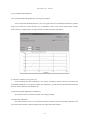
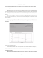
Table 2-1 List of CREPT-MCNP code menus
Main menu
File (F)
Sub menu
Example of function / Remarks
F1. Setting
MCNP path setting
F2. Exit
D1. Material
Material registration
D2. Detector
D3. Cover
Geometric definition for each
part
D4. Tray
D5. Support jig
Data (D)
D6. Measured sample
D7. Calculation area
Positional relationship between
the parts
D8. Geometry
D9. Source energy point
D10. Volume sample
Coordinates and intervals for
point source alignment
D11. Alignment of point source
C1. Efficiency-curves group A
Calculation
(C)
C2. Efficiency curve for volume sample without selfabsorption, representative point
Efficiency curves of a volume
sample by means of “point
integration”
C3. Efficiency curve for volume sample with and without
self-absorption
C4. Final efficiency curve
R1. Efficiency-curves group A
Efficiency curve at a specified
position is depicted graphically
R2. Efficiency-curves group B
Calculation
Results (R)
R3. Comparison of efficiency curve at a representative
point and that of volume sample without selfabsorption
R4. Contour map of parameter t
R5. Detailed contour map of parameter t around a
representative point
R6. Comparison of efficiency curves of a volume sample
by means of “point integration” and by MCNP
R7. Final efficiency curve
Window (W)
Help (H)
W1 - W4. Align in tiles, in piles, horizontally, vertically
H1. Help
H2. System version
−　−
7
For cross-checking
JAEA-Data/Code　2008-017
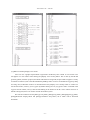
2.5 Operation Menus
2.5.1 [File] Menu
2.5.1.1 [File]-[Setting] Menu
Environmental settings required for operation are given in this menu.
(1) Language:
Select either English (United States) or Japanese (Japan) environment from the drop-down list. Note
that users can change the language whenever they need.
(2) MCNP file path:
A directory that includes the MCNP execution file need to be designated. By clicking the [...] button on
the right side of the line users can browse and select the necessary directory.
(3) MCNP file name:
A name for the MCNP execution file need to be entered. By clicking the [...] button on the right side of
the blank line users can browse and select the necessary file.
(4) Xsdir file path:
When version 5 MCNP is used leave this space blank. Otherwise (i.e. when version 4 MCNP is used),
the directory containing the “xsdir” file needs to be designated. Clicking the [...] button on the right side of the
blank line allows users to browse and select the necessary directory.
−　−
8
JAEA-Data/Code　2008-017
(5) Parameters for geometric visualization:
The CREPT-MCNP code uses the X-Windows system in illustrating a cross-sectional view of the
calculation geometries. Check the box if you wish to be notified before geometric depictions are drawn on the
display. Leave it blank if using version 4 MCNP.
2.5.1.2 [File]-[Exit] Menu
Selecting the [Exit] menu prompts the user a dialog box for a confirmation. Select [Yes] on that box to
exit.
2.5.2 [Data] Menu
There are eleven sub menus in the [Data] Menu.
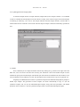
2.5.2.1 [Data]-[Material] Menu
Materials used in each detector, sample and sample container, etc. are defined with this menu.
Compositions and a density of each material are required for the definition. These data are stored as a material
database.
−　−
9
JAEA-Data/Code　2008-017
(1) Comment:
Space provided just for user made comments.
(2) Number of element(s):
Specify the number of element(s) or nuclide(s) which constitute a material. This will automatically
change the number of rows in the data grid at the bottom of the window.
(3) Density [g/cm3]:
Assign a density of the material in g cm-3.
(4) Specification of composition:
Select an input form to specify the material composition. Either “Atomic fraction” or “Weight fraction”
can be selected.
(5) [Data grid] Element, nuclide:
Specify elements or nuclides which constitute a material in ZA format. With the ZA format, a nuclide
with the atomic number of Z and the mass number of A is expressed as Z×1000+A. A is zero for a natural
element. (Example) H (hydrogen): 1000, Co (cobalt): 27000, 3H (tritium): 1003, and 60Co (cobalt 60): 27060.
−　10　−
10
JAEA-Data/Code　2008-017
(6) [Data grid] Fraction:
In accordance with the specification of composition, assign the appropriate fractions for the constituents
specified in the left columns. The sum of the fractions does not need to be unity, as the MCNP code will
renormalize the fractions if they do not sum to one.
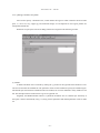
2.5.2.2 [Data]-[Detector] Menu
Parameters that specify the geometric configurations and materials of a detector are assigned in the
following window.
(1) Default:
First, a default style of a detector should be selected. By clicking the [...] button on the right side of the
blank line users can browse and select the necessary file. Parameter values of the default detector are then
modified to specify the intended detector. The default style itself cannot be modified in the GUI window but
can be modified or newly added in a text file. The format of the text file is described in Appendix A.8.
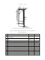
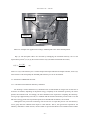
Originally, the CREPT-MCNP code has a p-type HPGe and an n-type HPGe as the default detectors.
Geometries of these detectors are shown schematically in Figs. 2-2 (for p-type HPGe) and 2-3 (for n-type
HPGe), along with their parameters and default parameter values in Tables 2-2 (for p-type HPGe) and 2-3 (for
n-type HPGe).
−　11　−
11
JAEA-Data/Code　2008-017
>@
>@
>@
>@
Fig. 2-2 Half sectional view of a default p-type HPGe (units in cm)
Table 2-2 Parameters, data type and default parameter values for a p-type HPGe
(File name: ge_TypeP.csv)
(1)
(2)
(3)
(4)
(5)
(6)
(7)
[8]
[9]
[10]
[11]
Parameter
Total length of detector [cm]
Distance from upper surface of detector case to upper surface of
Ge crystal [cm]
Length of Ge crystal [cm]
Thickness of dead layer [cm]
Thickness of end cap [cm]
Outer radius of Ge crystal [cm]
Outer radius of end cap [cm]
Material of Ge crystal
Material of contact pin
Material of mount-cup
Material of end cap
−　12　−
12
Data type
Floating-point
Default
11
Floating-point
0.43
Floating-point
Floating-point
Floating-point
Floating-point
Floating-point
Character
Character
Character
Character
7.9
0.09
0.13
2.925
3.5
-
>@
JAEA-Data/Code　2008-017
>@
5
5
>@
>@
>@
>@
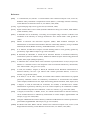
Fig. 2-3 Half sectional view of a default n-type HPGe (units in cm)
Table 2-3 Parameters, data type and default parameter values for an n-type HPGe
(File name: ge_TypeN.csv)
(1)
(2)
(3)
(4)
(5)
(6)
(7)
(8)
(9)
(10)
(11)
(12)
(13)
(14)
[15]
[16]
[17]
[18]
[19]
[20]
Parameter
Length of end cap [cm]
Distance from upper surface of detector case to upper surface of
Ge crystal [cm]
Length of Ge crystal [cm]
Distance from upper surface of Ge crystal to tip of contact pin
[cm]
Length of mount-cup [cm]
Thickness of dead layer [cm]
Thickness of end cap [cm]
Gap between end cap and protector [cm]
Thickness of protector (radial) [cm]
Thickness of window [cm]
Thickness of protector (top) [cm]
Thickness of mount-cup [cm]
Outer radius of Ge crystal [cm]
Outer radius of protector [cm]
Material of Ge crystal (including dead layer)
Material of mount-cup and contact pin
Material of end cap
Material of window
Filling material between end cap and protector
Material of protector
−　13　−
13
Data type
Floating-point
Default
11
Floating-point
0.45
Floating-point
7.6
Floating-point
2.47
Floating-point
Floating-point
Floating-point
Floating-point
Floating-point
Floating-point
Floating-point
Floating-point
Floating-point
Floating-point
Character
Character
Character
Character
Character
Character
9.6
0.00003
0.1
0.03
0.2
0.05
0.1
0.1
2.92
3.73
-
JAEA-Data/Code　2008-017
(2) [Data grid] Parameter:
Parameters which constitutes a detector are listed. Users cannot change, add or remove these parameters
(items) through the GUI window.
This rule is also applicable for the [Data]-[Cover] Menu, [Data]-[Tray] Menu, [Data]-[Support jig]
Menu, [Data]-[Measured sample] Menu and [Data]-[Calculation area] Menu, all of which will be described
hereinafter.
(3) [Data grid] Value:
Users can modify the parameter values if necessary. If the data type of a value is “matter”, select it from
the drop-down list. If no material is selected from the list, i.e. blank, the material is considered void in the
MCNP calculations.
This rule also holds true for the [Data]-[Cover] Menu, [Data]-[Tray] Menu, [Data]-[Support jig] Menu,
[Data]-[Measured sample] Menu and [Data]-[Calculation area] Menu, all of which will be described
hereinafter.
(4) [Button in toolbar] Show text file:
Clicking the [Show text file] button pops up the MCNP input file created by the code automatically. It is
helpful as reference although users cannot change the file in this window.
This rule also holds true for the [Data]-[Cover] Menu, [Data]-[Tray] Menu, [Data]-[Support jig] Menu,
[Data]-[Measured sample] Menu and [Data]-[Calculation area] Menu, all of which will be described
hereinafter.
−　14　−
14
JAEA-Data/Code　2008-017
(5) [Button in toolbar] Display cross section:
Users can view a graphic representation of geometric models they have created. A cross-section view
will appear in a new window after clicking the [Display cross section] button. This is done by the MCNP
geometry plotter (with the -ip option) and while X-Windows is being used, the plot window supports a variety
of interactive features (refer to the MCNP Manual [XM05]). When version 5 of MCNP and Cygwin [CY08]
are being used, X-Window needs to be launched before the [Display cross section] button is clicked. To
activate the window, in brief, (1) run Cygwin by double clicking its icon, (2) type the “startx” command in the
Cygwin console window, and (3) click the tab blinking at the bottom of the PC screen. When version 4 of
MCNP is being used, there is no need to start the X-Window system.
This rule also holds true for the [Data]-[Cover] Menu, [Data]-[Tray] Menu, [Data]-[Support jig] Menu,
[Data]-[Measured sample] Menu and [Data]-[Calculation area] Menu, all of which will be described
hereinafter.
−　15　−
15
JAEA-Data/Code　2008-017
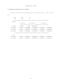
2.5.2.3 [Data]-[Cover] Menu
“Cover” refers to one of the parts around a detector. It might be used to protect a detector from
radioactive contamination or physical damage. Parameters to specify the geometric configuration and material
of the cover can be assigned in the following window.
−　16　−
16
JAEA-Data/Code　2008-017
(1) Default:
A default cover can be selected by clicking the [...] button on the right side of the blank line and users
can then browse and select the necessary file. The parameter values of the default cover are then modified to
specify the intended cover. And while the default style itself cannot be modified in the GUI window, it can be
modified or newly added using a text file of which the format is given in Appendix A.8.
Originally, the CREPT-MCNP code has a cylindrical closed-end cover as a default cover. The
geometry of the cover is shown schematically in Fig. 2-4, along with its parameters and default parameter
values in Table 2-4.
>@
>@
Fig. 2-4 Half sectional view of a default cover
Table 2-4 Parameters, data type and parameter values of the default cover
(File name: cover.csv)
(1)
(2)
(3)
(4)
[5]
[6]
Parameter
Thickness of cover (top) [cm]
Length of cover [cm]
Inner radius of cover [cm]
Outer radius of cover [cm]
Material of cover
Filling material of space laying inside cover
Data type
Floating-point
Floating-point
Floating-point
Floating-point
Character
Character
−　17　−
17
Default
0.2
12
3.7
3.8
-
JAEA-Data/Code　2008-017
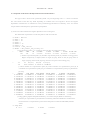
2.5.2.4 [Data]-[Tray] Menu
“Tray” is another part around a detector and may be used as a stage to set a sample to be measured
above the detector. Parameters to specify the geometric configuration and material of the tray can be assigned
in the following window.
(1) Default:
A default style of a tray is selected by clicking the [...] button on the right side of the blank line. Users
can browse and select the intended file. Parameter values of the default tray are then modified to specify the
intended tray. The default style itself cannot be modified on the GUI window, but it can be modified or newly
added in a text file. The description format of the file is in Appendix A.8.
Originally, the CREPT-MCNP code has a plate-shaped tray as a default style tray. Geometry of the tray
is shown schematically in Fig. 2-5, along with its parameters and default parameter values in Table 2-5.
−　18　−
18
JAEA-Data/Code　2008-017
>@
Fig. 2-5 Half sectional view of a default tray
Table 2-5 Parameters, data type and parameter values of the default tray
(File name: disk.csv)
(1)
(2)
[3]
Thickness of tray [cm]
Radius of tray [cm]
Material of tray
Parameter
Data type
Floating-point
Floating-point
Character
−　19　−
19
Default
0.2
16
-
JAEA-Data/Code　2008-017
2.5.2.5 [Data]-[Support jig] Menu
“Support jig” is another part around a detector. It might be used as an attachment to join the end cap of a
detector and a cover. Parameters to specify the geometric configuration and material of the support jig can be
assigned in the following window.
(1) Default:
A default style of a support jig is selected by clicking the [...] button on the right side of the blank line.
Users can browse and select the necessary file. The parameter values of the default support jig are then
modified to specify the intended support jig. The default style itself cannot be modified in the GUI window,
but it can be modified or newly added in a text file. The description format of the text file is given in Appendix
A.8.
Originally, the CREPT-MCNP code has an annular support jig as a default style. The geometry of the
support jig is shown schematically in Fig. 2-6, along with its parameters and default parameter values in Table
2-6.
−　20　−
20
JAEA-Data/Code　2008-017
>@
Fig. 2-6 Half sectional view of a default support jig
Table 2-6 Parameters, data type and parameter values of the default support jig
(File name: annular.csv)
(1)
(2)
(3)
(4)
[5]
[6]
Parameter
Thickness of support jig (top) [cm]
Total height of support jig [cm]
Inner radius of support jig [cm]
Mid radius of support jig [cm]
Outer radius of support jig [cm]
Material of support jig
Data type
Floating-point
Floating-point
Floating-point
Floating-point
Floating-point
Character
−　21　−
21
Default
0.5
2
3
3.6
3.7
-
JAEA-Data/Code　2008-017
2.5.2.6 [Data]-[Measured sample] Menu
A measured sample consists of sample material (sample matrix) and a sample container. It is modelled
in order to calculate the self-absorption correction factors. Usually, users create two types of measured sample
in obtaining an efficiency curve. One is with sample material and with sample container, and the other is
without either of them. With this version of the code the shape of sample is limited to rotationally symmetrical
ones.
(1) Default:
First, a default style of a sample should be selected. By clicking the [...] button on the right side of the
blank line, users can browse and select the necessary file. Parameter values of the default sample are then
modified to specify the intended sample. The default style itself cannot be modified in the GUI window, but it
can be modified or newly added in a text file. The description format of the text file is given in Appendix A.8.
Originally, the CREPT-MCNP code has a cylindrical sample and the Marinelli-shaped [IE78] sample as
default style samples. The geometries of these samples are shown schematically in Figs. 2-7 (for the
cylindrical sample) and 2-8 (for the Marinelli-shaped sample), along with their parameters and default
parameter values in Tables 2-7 (for the cylindrical sample) and 2-8 (for the Marinelli-shaped sample).
−　22　−
22
JAEA-Data/Code　2008-017
>@
>@
Fig. 2-7 Half sectional view of a default style cylindrical sample
Table 2-7 Parameters, data types and parameter values of the default cylindrical sample
(File name: cylinder.csv)
(1)
(2)
(3)
(4)
(5)
[6]
[7]
Parameter
Thickness of sample container (bottom) [cm]
Distance from basal surface of sample container to top surface of
sample [cm]
Height of sample container [cm]
Inner radius of sample container [cm]
Outer radius of sample container [cm]
Material of sample container
Material of volume sample
−　23　−
23
Data type
Floating-point
Default
0.2
Floating-point
5
Floating-point
Floating-point
Floating-point
Character
Character
16
4
4.2
-
JAEA-Data/Code　2008-017
>@
>@
Fig. 2-8 Half sectional view of a default Marinelli-shaped sample
Table 2-8 Parameters, data types and parameter values of the default Marinelli-shaped sample
(File name: Marinelli.csv)
(1)
(2)
(3)
(4)
(5)
(6)
(7)
(8)
[9]
[10]
Parameter
Height of volume sample [cm]
Height of sample container [cm]
Length of sub-part of Marinelli beaker (base to base) [cm]
Inner radius of sub-part of Marinelli beaker [cm]
Outer radius of sub-part of Marinelli beaker [cm]
Outer radius of basal surface of sample container [cm]
Outer radius of top surface of sample container [cm]
Thickness of sample container [cm]
Material of sample container
Material of volume sample
−　24　−
24
Data type
Floating-point
Floating-point
Floating-point
Floating-point
Floating-point
Floating-point
Floating-point
Floating-point
Character
Character
Default
8.9
8.9
7.6
4.15
6.85
7.25
7.65
0.2
-
JAEA-Data/Code　2008-017
2.5.2.7 [Data]-[Calculation area] Menu
Users need to specify “calculation area”, which denotes the region in which a detector and all of other
parts, i.e., the cover, tray, support jig and measured sample, are encompassed. In that region photons are
transported with MCNP.
Parameters to specify the area and its filling material are assigned on the following window.
(1) Default:
A default calculation area is selected by clicking the [...] button on the right side of the blank line. Users
can browse and select the intended file. The parameter values are then modified to specify the intended region.
The default style itself cannot be modified in the GUI window, but it can be modified or newly added in a text
file. The description format of the text file is given in Appendix A.8.
Originally, the CREPT-MCNP code has a cylindrical calculation area as a default style. Geometry of
the region is shown schematically in Fig. 2-9, along with its parameters and default parameter values in Table
2-9.
−　25　−
25
JAEA-Data/Code　2008-017
^`
= FP
>@
^`
Fig. 2-9 Half sectional view of a default style calculation area
Table 2-9 Parameters, data types and parameter values of the default calculation area
(File name: cylinder.csv)
{1}
{2}
(3)
[4]
Parameter
Lower limit of region in Z direction [cm]
Upper limit of region in Z direction [cm]
Radius of calculation area [cm]
Material of calculation area
Data type
Floating-point
Floating-point
Floating-point
Character
−　26　−
26
Default
-13
17
17
-
JAEA-Data/Code　2008-017
2.5.2.8 [Data]-[Geometry] Menu
In the [Data]-[Geometry] Menu, users can complete a geometric model used in the MCNP calculations.
This is done by selecting the parts used, i.e., a detector, cover and/or measured sample etc., and by providing
positional relationships among the selected parts, in the following window.
(1) Select parts:
Of the six different types of parts, users must select those necessary to create a geometric model by
checking the checkboxes and assigning necessary file names by clicking the [...] buttons. Note that because a
detector and a calculation area are both essential to the calculations, their file names must be assigned without
exception.
Attention should be paid when users are creating the geometric models for the self-absorption
correction factor calculations. In calculations of the self-absorption correction factor, users will need to create
two types of geometric models; one is with sample material and with sample container, and the other is
without either of them. In the case users use a tray for a measurement of a volume sample, the tray should be
selected in a calculation with sample material and a sample container, and should be checked off for a
calculation without either of them, unless the tray is included in the calculation geometry for obtaining
“efficiency-curves group A”. In the calculations of the efficiency-curves group A, normally, the tray should be
considered to be part of a sample container, rather than as part of a detector, because it intervenes with the
setting of the Marinelli-shaped sample.
−　27　−
27
JAEA-Data/Code　2008-017
Once a geometric model has been saved in a file, it can be re-opened and re-edited in the window. Note,
however, that any change given on parts through the [Data]-[Cover] Menu, [Data]-[Tray] Menu, [Data][Support jig] Menu, [Data]-[Measured sample] Menu and [Data]-[Calculation area] Menu (These data are
stored in the [\work\parts] folder.) is not reflected automatically just by opening a geometric model file. If any
of these parts were changed, users must click the [...] buttons and reselect the file to reflect the changes in the
geometric model.
(2) [Tab] Offset value:
The positional relationships among the selected parts are set with the “Offset value” tab. There are a
total of eleven parameters, but only those related to the selected parts are listed in the data grid. The eleven
parameters are as follows.
1) Z-position of top surface of cover (Default value: -0.0001)
2) Gap between cover and detector (Default value: 0)
3) Gap between cover and support jig (Default value: 0)
4) Gap between cover and measured sample (Default value: 0)
5) Gap between tray and cover (Default value: 0)
6) Z-position of top surface of detector (Default value: -0.0001)
7) Gap between detector and measured sample (Default value: 0)
8) Gap between tray and detector (Default value: 0)
9) Gap between support jig and detector (Default value: 0)
10) Gap between tray and measured sample (Default value: 0)
11) Z-position of top surface of tray (Default value: -0.0001)
Ensure that the Z-position of a selected part has been correctly set, so that the detector locates the same
position between when the efficiency-curves group is to be calculated and when the self-absorption correction
factors are to be calculated.
(3) [Tabs] Measured sample, Support jig, Tray, Cover, Detector, Calculation area
The parameters and their values are listed for reference. Users can change these parameter values
temporarily using these tabs but the change or changes are not reflected in the original data which has been
stored in the [\work\parts] folder.
−　28　−
28
JAEA-Data/Code　2008-017
2.5.2.9 [Data]-[Source energy point] Menu
In the [Data]-[Source energy point] Menu, a data group is set in terms of energy points for a virtual
multi-energy photon source, and of the region of interest (ROI) for detections of photons at a detector.
(1) Number of energy points:
Assign the number of energy points to be used in the MCNP calculations. The number of rows in the
data grid will change in relation to that number.
(2) Energy region of interest (%):
The energy region of interest (ROI) is a region related to the pulse-height spectrum tally (the “F8 tally”)
in MCNP. Default value for the energy ROI is 8 %. For example, in the case the value is set at 8 %, a photon
with initial energy 1 MeV will be tallied if it has deposited energy between 0.92 and 1.08 MeV on a detector.
The value will be used with each individual energy point.
(3) Energy (MeV):
Photon energy points in MeV units must be assigned in ascending order. The energy points must be
between 0.01 MeV and 10 MeV.
−　29　−
29
JAEA-Data/Code　2008-017
2.5.2.10 [Data]-[Volume sample] Menu
The conditions of a volume sample (source conditions) are set in order to estimate the self-absorption
correction factors.
−　30　−
30
JAEA-Data/Code　2008-017
(1) [Tab] General; Configuration of a source:
In this version of the code, only a cylindrical volume sample with its axis coinciding with the detector
axis, and of homogeneous material, can be treated. Users, therefore, should select “Cylinder (on z-axis,
uniform distribution)”.
(2) [Tab] Configuration; Number of volume source(s):
Users will not be able to change this number if “Cylinder (on z-axis), uniform distribution” was selected
at the “Configuration of a source” item in the “General” tab.
(3) [Tab] Configuration; [Data grid]:
Users should provide a radius and positions (in Z-direction) of a cylindrical volume sample from which
photons will be emitted (refer also to (4)).
(4) [Tab] General; [Checkbox] Particles emitted from overlapped area:
Should be checked when users intend to make photons be emitted from an overlapping region by a
cylindrical region set with the “Configuration” tab and by a measured sample which is set with the [Data][Measured sample] Menu.
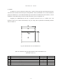
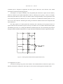
Examples of this concept are schematically shown in Fig. 2-10. In the case the cylindrical region is
larger than the measured sample, as in pattern A of the figure, the source region will be identical to the
measured sample. If the cylindrical region does not encompass the measured sample, as in pattern B, then the
source region is the region that overlaps the two regions. In most cases, users will set the source region as in
pattern A, and note that they have provided the parameters for the cylindrical region that are the same or
somewhat larger, but not that larger, than the measured sample. Such settings will help improve the
computational efficiency of sampling a source position with the Monte Carlo calculation.
(5) [Tab] General; File name (energy points):
A file defining a data group of source energy points should be selected by clicking the [...] button on
the right side of the blank line. The file can be created with the [Data]-[Source energy point] Menu and users
can browse and select the created file.
(6) [Tab] Configuration; Number of volume source(s):
In this version of the code, users cannot change this setting if “Cylinder (on z-axis), uniform
distribution” was selected in the “Configuration of a source” item of the “General” tab.
−　31　−
31
JAEA-Data/Code　2008-017
0HDVXUHGYROXPHVDPSOH
0HDVXUHGYROXPHVDPSOH
&\OLQGULFDOUHJLRQ
&\OLQGULFDOUHJLRQ
6RXUFHUHJLRQ
VKDGHG
6RXUFHUHJLRQ
VKDGHG
3DWWHUQ%
3DWWHUQ$
Fig. 2-10 Half sectional view of the positional relationship of the cylindrical region and measured sample
−　32　−
32
JAEA-Data/Code　2008-017
2.5.2.11 [Data]-[Alignment of point source] Menu
In this menu, a group of grid points (lattice points) is set for obtaining “efficiency-curves group A”. The
lattice points distributes around a detector in a two-dimensional (R-Z) space which includes a detector axis.
(1) R-coordinate, Z-coordinate [cm]:
Users should set R and Z ranges in which the virtual point source is placed. Note that the value in the
left textbox is smaller than that in the right.
(2) Number of partitions for R, Number of partitions for Z:
Assign the number of partitions (division numbers) for each range set in either the R-coordinate or Zcoordinate columns. When the number of partitions is assigned as n, the number of lattice points becomes n
+1. (Example) In the case a range of “0.0 to 4.0” is divided by the number of partitions “2”, then three lattice
points are set at “0.0”, “2.0” and “4.0”.
(3) Additional coordinate point(s) for R, Additional coordinate point(s) for Z:
Users can set coordinate point(s) in addition to the lattice points set in (1) and (2). More than one extra
point can be set by entering a comma in between two values. (Example) “3.4,4.5,5.6”. The additional
−　33　−
33
JAEA-Data/Code　2008-017
coordinate point is designed to supplement the lattice points which have fixed intervals. This should
specifically be used for the following purposes.
One purpose is to improve reliability in the interpolated peak efficiencies at points near the detector,
which are obtained by the Spline-interpolation with the “efficiency-curves group A” data. For example,
because the peak efficiency in the vicinity of a detector tends to change drastically in the range between 0 and
2 cm from the top surface of a detector (or a cover), it is effective to set additional coordinate points at 0.5 cm
and 1.0 cm in the Z direction. Introducing this setting will reduce the difference between the interpolated and
actual efficiencies.
The other purpose is to obtain point-source efficiency data (“efficiency-curves group B” data) at a
region which intervenes the outermost part (an end cap of a detector or cover) and the innermost lattice points
(the shaded region in Fig. 2-11). Setting the additional coordinate points just over the outermost part (line B in
the figure) enables the Spline-interpolation in a region between the added points and the original lattice points.
&DOFXODWLRQ
DUHD
$
2ULJLQDOODWWLFH
SRLQWV
'HWHFWRU
%
Fig. 2-11 Lattice points around a detector (half sectional view)
(4) Configuration of a source:
At the time of writing, only a point source without a source holder had been verified as an option. Users,
therefore, should select “Sheer point” at this stage. In most cases this will bring about reasonable results.
−　34　−
34
JAEA-Data/Code　2008-017
2.5.3 [Calculation] Menu
2.5.3.1 [Calculation]-[Efficiency-curves group A] Menu
With this menu, a series of Monte Carlo calculations is carried out in order to obtain the “Efficiencycurves group A”.
(1) File name (Calculation geometry):
A file defining a geometric model which includes a detector, a calculation area, and other optional parts
(possibly a cover and/or support jig, but usually excludes a tray because it hampers the setting of a Marinellishaped sample) should be selected by clicking the [...] button on the right side of the blank line. The file can be
created in the [Data]-[Geometry] Menu and users can browse and select the created file.
(2) File name (Energy points):
A file defining a data group of the source energy points should be selected by clicking the [...] button on
the right side of the blank line. The file can be created in the [Data]-[Source energy point] Menu and users can
browse and select the created file.
−　35　−
35
JAEA-Data/Code　2008-017
(3) File name (Calculation area):
A file defining the lattice point should be selected by clicking the [...] button on the right side of the
blank line. The file can be created in the [Data]-[Alignment of point source] Menu and users can browse and
select the created file.
(4) [Checkbox] Recalculate:
Users can recalculate a series of calculations by checking the checkbox. This option takes effect by
assigning an uncompleted output file located in the [\work\effA] directory and allows users to resume any
calculations which has been accidentally or purposely suspended.
(5) Number of particles:
The number of source particles per batch (refer to the following (6) and (7) for more details on the
batch) is set in the textbox. The default value is 100000.
(6) Statistical accuracy (termination condition):
Assign the statistical accuracy to terminate a calculation. An MCNP calculation is carried out for
obtaining a peak efficiency at each lattice point (or at the additional coordinate point) and for each energy
point, but the calculation actually consists of several sub-calculations which are segmented into source
particles batches. That is, the sub-calculations are automatically repeated until the statistical accuracy is equal
or less than the assigned value. The default value is 0.01.
(7) Maximum calculation time (min):
Assign the maximum calculation time to terminate a calculation. This option is useful for calculations
that users expect long calculation time to reduce the statistical accuracy, such as those with predominant
interactions between photons and high-shielding material. A calculation consists of several sub-calculations
which are segmented into source particle batches. Sub-calculations are automatically repeated until the
calculation time reaches the assigned value. In other words, it automatically stops once the time has been
reached, irrespective of the statistical accuracy value set in (6). The default time value is 0, and in this case a
calculation stops based only on the statistical accuracy. Note that the maximum calculation time must be set
for one MCNP calculation, through which an efficiency value for a point source with photon energy E, located
at P(r,z), is obtained.
(8) Output file name (efficiency-curves group A):
An output file name must be assigned by clicking the [...] button on the right side of the blank line.
Users can browse and select an existing file in the case the “Recalculate” checkbox is checked, otherwise a
new file name must be given. The extension for this type of file is “.out”.
−　36　−
36
JAEA-Data/Code　2008-017
(9) [Button] Run (or Stop):
By pressing the run button users can start or resume a series of calculations. Progress of calculations is
displayed in the window. Users can suspend a series of calculations by pressing the stop button.
2.5.3.2 [Calculation]-[Efficiency curve for volume sample without self-absorption, representative point] Menu
The main purpose of this menu is to calculate the following data, based on the data of the efficiencycurves group A.
· Efficiency-curves group B (Spline-interpolated data of the efficiency-curves group A)
· Efficiency-curves group C (finely Spline-interpolated data of the efficiency-curves group A)
· Efficiency curve of an air-equivalent measured volume sample (volume weighted average of the
efficiency-curves group C)
· Position of a representative point (selected from the data of efficiency-curves group B)
(1) File name (efficiency-curves group A):
A file containing the data of efficiency-curves group A should be selected. The file can be created in the
[Calculation]-[Efficiency-curves group A] Menu. By clicking the [...] button on the right side of the blank line
users can browse and select the intended file.
−　37　−
37
JAEA-Data/Code　2008-017
(2) Number of partitions for R:
A division number should be provided to calculate the data of the efficiency-curves group B from that
of the efficiency-curves group A. For example, in the case the number of the partitions which is set in the
[Data]-[Alignment of point source] Menu is 9 and this value is 20, the lattice points for the efficiency curves
group becomes 161 (= (9-1)×20 +1). The default value is 20.
(3) Number of partitions for Z:
Same as above.
(4) [Checkbox] Save data of efficiency-curves group:
Users should check the checkbox if they want to keep the data of efficiency-curves group B in a file. In
the case, an output file name must be assigned by clicking the [...] button on the right side of the blank line.
(5) [Hidden menu] File name (angular dependence of efficiency):
This option cannot currently be used. Select nothing.
(6) Number of sub-partitions for R:
An additional division number should be provided to calculate the data of the efficiency-curves group C
from that of the efficiency-curves group A (not B). The number should be given to the lattice interval used in
the efficiency-curves group B. For example, in the case the number of the partitions of the efficiency-curves
group B is 161 and the value given is 10, the number of lattice points in the efficiency-curves group C will be
1601 (= (161-1)×10 +1). The default value is 10.
(7) Number of sub-partitions for Z:
Same as above.
(8) File name (volume sample):
A file containing the data of volume sample (volume source) should be selected. The file is created in
the [Data]-[Volume sample] Menu. By clicking the [...] button on the right side of the blank line, users can
browse and select the necessary file.
Users are strongly recommended to check over that the position (and size) of a volume sample and
detector coincides with the geometries which are used in the calculation of the efficiency-curves group A.
−　38　−
38
JAEA-Data/Code　2008-017
(9) File name (calculation geometry):
A file containing a data of calculation geometry for the calculation of the self-absorption correction
factor should be selected. The file is created in the [Data]-[Geometry] Menu. Users will possibly find two
types of files to select. One is a file with sample material and the other is that without sample material (airequivalent sample). Users can select either, because they will give the same result. By clicking the [...] button
on the right side of the blank line, users can browse and select the necessary file.
Users are strongly recommended to check over that the position (and size) of a volume sample and
detector in the selected file coincides with the geometries which are used in the calculation of the efficiencycurves group A, and with the volume sample mentioned in (9). In the case the “Particles emitted from
overlapped area” checkbox (see [Data]-[Volume sample] Menu) was checked when the volume sample file
was created, this option ((9) calculation geometry) is not activated.
(10) Output file name (data of representative point):
An output file name must be assigned by clicking the [...] button on the right side of the blank line. The
extension for this type of file is “.out”.
(11) [Checkbox] Specification of a cut plane for distribution of t:
This option is not currently available. Leave unchecked.
(12) [Button] Run:
A calculation starts by pressing the run button. It will typically take a few minutes to finish if both files
((8) volume sample and (9) calculation geometry) are involved, but less if only (8) volume sample file is used
for discrimination of a source region from the efficiency-curves group C.
−　39　−
39
JAEA-Data/Code　2008-017
2.5.3.3 [Calculation]-[Efficiency curve for a volume sample with and without self-absorption] Menu
With this menu, a series of Monte Carlo calculations is carried out in order to obtain the self-absorption
correction factors. This includes calculations of the,
· The efficiency curve of a volume source with sample material and sample container,
· The efficiency curve of a volume source without sample material and without sample container (airequivalent sample).
(1) File name (calculation geometry) (with material/container):
A file containing the data of calculation geometry for the calculation of the self-absorption correction
factor should be selected. The file is created in the [Data]-[Geometry] Menu. By clicking the [...] button on the
right side of the blank line, users can browse and select the necessary file.
Users are strongly recommended to check over that the position (and size) of a volume sample and
detector in the selected file coincides with the geometries which are used in the calculation of the efficiencycurves group A, and with the volume sample mentioned in the following (3).
−　40　−
40
JAEA-Data/Code　2008-017
(2) File name (calculation geometry) (without material/container):
A file containing the data of calculation geometry for the calculation of the self-absorption correction
factor should be selected. The file is created in the [Data]-[Geometry] Menu. By clicking the [...] button on the
right side of the blank line, users can browse and select the necessary file.
Users are strongly recommended to check over that the position (and size) of a volume sample and
detector in the selected file coincides with the geometries which are used in the calculation of the efficiencycurves group A, and in the volume sample mentioned in the following (3).
Confirm that in the case users use a tray for a measurement of a volume sample, the tray should be
removed, or filled with air, for a calculation without sample material and without container, unless the tray is
included in the calculation geometry for obtaining the efficiency-curves group A.
(3) File name (volume sample):
A file containing the data of volume sample (volume source) should be selected. The file is created in
the [Data]-[Volume sample] Menu. By clicking the [...] button on the right side of the blank line, users can
browse and select the necessary file.
Users are strongly recommended to check over that the position (and size) of a volume sample and
detector coincides with the geometries which are used in the calculation of the efficiency-curves group A.
(4) [Data grid] Arbitrary uncertainty:
Each calculated efficiency value is accompanied by its statistical uncertainty, which is automatically
estimated by the MCNP code. There is, however, the non-statistical uncertainty other than the statistical one.
The non-statistical uncertainty originates from various factors related to the calculation, e.g., reliability in the
geometric model, cross section data and so on. Users can assign non-statistical uncertainties as their best
estimates in the data grid. The uncertainties should be set in their relative values. If users wish to put uniform
values in the data grid irrespective of the source energy, it can be done by assigning the value in the “Set all”
textbox.
(5) Number of particles:
The number of source particles per batch (refer to the following (6) and (7) with regard to the batch) is
set in the textbox. The default value is 100000.
(6) Statistical accuracy (termination condition):
Assign the statistical accuracy at which to terminate a calculation. Each calculation consists of several
sub-calculations which are segmented into source particle batches. That is, the sub-calculations are
automatically repeated until the statistical accuracy is equal or less than the assigned value. The default value
is 0.01.
−　41　−
41
JAEA-Data/Code　2008-017
(7) Maximum calculation time (min):
Assign the maximum calculation time to terminate a calculation. This option is useful for calculations
which users expect a long calculation time to reduce the statistical accuracy, such as those with predominant
interactions between photons and high-shielding material. A calculation consists of several sub-calculations
which are segmented into source particles batches. The sub-calculations are automatically repeated until the
calculation time reaches the assigned value. In other words, it automatically stops once the time has been
reached, irrespective of the statistical accuracy value set in (6). The default value for the time is 0, and in this
case a calculation stops based only on the statistical accuracy. Note that the maximum calculation time must
be set for one MCNP calculation, through which an efficiency value for a point source with photon energy E,
located at P(r,z), is obtained.
(8) Output file of an efficiency curve (with material/container):
An output file name must be assigned by clicking the [...] button on the right side of the blank line. The
extension for this type of file is “.out”.
(9) Output file of an efficiency curve (without material/container):
An output file name must be assigned by clicking the [...] button on the right side of the textbox. The
extension for this type of file is “.out”.
(10) [Button] Run:
A series of calculations starts by pressing the run button. Progress of calculations is displayed on the
window. Users can stop the calculations by pressing the stop button but do note there is no “recalculate”
option.
−　42　−
42
JAEA-Data/Code　2008-017
2.5.3.4 [Calculation]-[Final efficiency curve] Menu
In this menu, the efficiency curve of a volume sample (the final efficiency curve) is calculated by
multiplying the measured efficiency curve at the representative point by the calculated self-absorption
correction factor.
(1) File name (Efficiency curve of a volume sample with material/container):
A file containing the efficiency curve data of a volume sample (with both material and container)
should be selected. By clicking the [...] button on the right side of the blank line, users can browse and select
the necessary file.
(2) File name (representative point):
A file containing calculated results of the representative point should be selected. By clicking the [...]
button on the right side of the blank line, users can browse and select the necessary file.
(3) File name (measured efficiency):
A file containing measured efficiency curve data with a point standard source should be selected. Users
must prepare the file in the format shown in Appendix A.7. The file should be stored in the [\work\meas]
folder and will appear through clicking the [...] button on the right side of the blank line.
If the energy points in this file differ from those used in (1) or (2), the energy point group used in this
(measured) data are adopted to the output file (4). This is done based on the Spline-interpolation or
extrapolation.
−　43　−
43
JAEA-Data/Code　2008-017
(4) Output file name (final efficiency curve):
An output file name must be assigned by clicking the [...] button on the right side of the blank line. The
extension for this type of file is “.out”.
(5) Efficiency curve of a volume sample without material/container:
A file containing the efficiency curve data of a volume sample (without material and without container)
should be selected. By clicking the [...] button on the right side of the blank line, users can browse and select
the necessary file.
(6) Uncertainty in point-source setting [mm]:
This option is used to take in to account any uncertainty in the setting position of a standard point source
at the representative point. The uncertainty, r, should be given in millimetres. The resultant uncertainty in the
efficiency will be the maximum difference between the calculated efficiency at the original point and that at a
point which has a distance r from the original point.
(7) [Button] Run:
Calculation starts by pressing the run button, and it will finish instantly.
−　44　−
44
JAEA-Data/Code　2008-017
2.5.4 [Calculation Results] Menu
2.5.4.1 [Calculation Results]-[Efficiency-curves group A] Menu
Users can plot the calculated efficiency curve in a graph on the screen. Both the horizontal axis (photon
energy) and vertical axis (peak efficiency) are in logarithmic scales. Users cannot change ranges of these
scales. However, if needed, users can export the data to a Microsoft Excel spreadsheet.
(1) File name (efficiency-curves group A):
A file containing the data of efficiency-curves group A should be selected. The file is created in the
[Calculation]-[Efficiency-curves group A] Menu. By clicking the [...] button on the right side of the blank line,
users can browse and select the necessary file.
(2) File name (angular dependence of efficiency):
This option cannot be used at the moment. Leave the space blank.
(3) R-direction, Z-direction:
The lattice number in the R (or Z) direction should be selected. The corresponding coordinate value
(cm) for the lattice number will then be displayed to the right of the lattice number.
−　45　−
45
JAEA-Data/Code　2008-017
(4) [Button] Call EXCEL:
By clicking this button, the efficiency data and graph can be exported to a Microsoft Excel*1
spreadsheet as follows.
2.5.4.2 [Calculation Results]-[Efficiency curves group B] Menu
Users can plot the calculated efficiency curve in a graph on the screen. Both the horizontal axis (photon
energy) and vertical axis (peak efficiency) are in logarithmic scales. Users cannot change ranges of these
scales. However, if needed, users can export the data to a Microsoft Excel spreadsheet.
*1
Microsoft Excel® version 2002 or later is necessary.
−　46　−
46
JAEA-Data/Code　2008-017
(1) File name (efficiency-curves group B):
A file containing the data of efficiency-curves group B should be selected. The file is created in the
[Calculation]-[Calculation of efficiency curve for volume sample without self-absorption, representative
point] Menu. By clicking the [...] button on the right side of the blank line, users can browse and select the
necessary file.
(2) File name (angular dependence of efficiency):
This option cannot be used at the moment. Leave the space blank.
(3) R-direction, Z-direction:
The lattice number in the R (or Z) direction should be selected. The corresponding coordinate value
(cm) for the lattice number will then be displayed to the right of the lattice number.
(4) [Button] Call EXCEL:
By clicking this button, the efficiency data and graph can be exported to a Microsoft Excel® spreadsheet.
−　47　−
47
JAEA-Data/Code　2008-017
2.5.4.3 [Calculation Results]-[Comparison of efficiency curve at a representative point and that of volume
sample] Menu
With this menu, users can compare two types of efficiency curves, one being a calculated efficiency
curve at the representative point (red curve in the figure) while the other is that of a volume sample without
any self-absorption effect (blue curve). Both curves are determined through the data of efficiency-curves
group C.
The two curves should have similarity in their shapes and magnitudes. Degree of agreement between
two curves means the minimum t (%). If these curves do not show similarity, the user should check over the
source conditions.
Both the horizontal axis (photon energy) and vertical axis (peak efficiency) are in logarithmic scales.
Users cannot change ranges of these scales. However, if needed, users can export the data to a Microsoft Excel
spreadsheet.
(1) File name (representative point):
A file containing calculated results of the representative point should be selected. By clicking the [...]
button on the right side of the blank line, users can browse and select the intended file.
(2) [Button] Call EXCEL:
By clicking this button, the efficiency data and graph can be exported to a Microsoft Excel® spreadsheet.
−　48　−
48
JAEA-Data/Code　2008-017
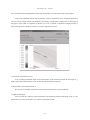
2.5.4.4 [Calculation Results]-[Contour map of parameter t] Menu
In this menu, a contour map of the parameter t which is calculated in the [Calculation]-[Efficiency curve
for volume sample without self-absorption, representative point] Menu is displayed in an R-Z graph. In the
graph, a region which is occupied by a detector (or a cover) is blacked out.
(1) File name (representative point):
A file containing calculated results of the representative point should be selected. By clicking the [...]
button on the right side of the blank line, users can browse and select the intended file.
(2) Representative point and parameter t:
The values of a calculated representative point and parameter t at the point are displayed.
(3) [Button] File output:
Users can refer the t values by pressing this button. The output file includes a data group of (R, Z, t) in a
tabular format.
−　49　−
49
JAEA-Data/Code　2008-017
2.5.4.5 [Calculation Results]-[Detailed contour map of parameter t around a representative point] Menu
In this menu, a detailed contour map of parameter t which is calculated in the [Calculation]-[Efficiency
curve for volume sample without self-absorption, representative point] Menu is displayed in an R-Z graph. In
the graph, a region which is occupied by a detector (or a cover), if present, is blacked out. Displayed range in
the R and Z directions is limited to within ±2 cm from a representative point.
(1) File name (representative point):
A file containing calculated results of the representative point should be selected. By clicking the [...]
button on the right of the blank line, users can browse and select the necessary file.
(2) Representative point and parameter t:
The values of a calculated representative point and parameter t at the point are displayed.
(3) [Button] File output:
Users can refer the t values by pressing this button. The output file includes a data group of (R, Z, t) in a
tabular format. R and Z are limited to ±2 cm from a representative point.
−　50　−
50
JAEA-Data/Code　2008-017
2.5.4.6 [Calculation Results]-[Comparison of efficiency curves of a volume sample by means of “point
integration” and by MCNP] Menu
In this menu, users can compare two efficiency curves. Both are efficiency curves of an air-equivalent
volume sample, but processes used to estimate each curve differ. One curve (red curve in the figure) is
obtained by means of the “point integration” with the data of efficiency-curves group C, and the other (blue
curve) is calculated by simulating volume source (bulk sample) in MCNP. These two efficiency curves may
well be identical, if the accuracy of the Spline-interpolation was sufficient. Otherwise, users should check over
the geometric models used for the calculations. Both the horizontal axis (photon energy) and vertical axis
(peak efficiency) are in logarithmic scales. Users cannot change ranges of these scales. However, if needed,
users can export the data to a Microsoft Excel spreadsheet.
(1) File name (representative point):
A file containing the calculated results of the representative point should be selected. By clicking the
[...] button on the right side of the blank line, users can browse and select the necessary file.
(2) File name (efficiency curve for volume sample without material/container):
A file containing the efficiency curve data of a volume sample (without material and without container)
should be selected. By clicking the [...] button on the right side of the blank line, users can browse and select
the necessary file.
−　51　−
51
JAEA-Data/Code　2008-017
(3) [Button] Call EXCEL:
By clicking this button, the efficiency data and graph can be exported to a Microsoft Excel® spreadsheet.
2.5.4.7 [Calculation Results]-[Final efficiency curve] Menu
Users can plot on a graph the efficiency curve which was determined by the representative point method
(final efficiency curve; shown in blue line). In the graph, a measured efficiency curve (red curve) at a
representative point is also shown for comparison.
Both the horizontal axis (photon energy) and vertical axis (peak efficiency) are in logarithmic scales.
Users cannot change the ranges of these scales. However, if needed, users can export the data to a Microsoft
Excel spreadsheet.
(1) File name (final efficiency curve):
A file containing the final efficiency curve data should be selected. The file is created in the
[Calculation]-[Final efficiency curve] Menu. By clicking the [...] button on the right side of the blank line,
users can browse and select the necessary file.
(2) [Button] Call EXCEL:
By clicking this button, the efficiency data and graph can be exported to a Microsoft Excel® spreadsheet.
−　52　−
52
JAEA-Data/Code　2008-017
3 Efficiency Calibration of Radioactivity Measuring Instrument with the Representative
Point Method
3.1 Present Status of Efficiency Calibration
In order to estimate the radioactivity in a volume sample nondestructively, the gamma-ray spectrometry
method with a germanium semi-conductor detector is generally used. In the method, the peak efficiency curve
must be evaluated in advance of the measurement. Procedures for obtaining the peak efficiency curve are
called “efficiency calibration”. There are many studies related to the efficiency calibration for radioactivity
quantification for a volume sample. Most of them are classified into three types such as; comparative
measurement with a standard volume source, analytical calculation, and the Monte Carlo calculation.
In the first method, the comparative measurement, the peak efficiency is estimated from the peak
counting rate measured by a germanium detector on which a standard volume source is set. And for this the
standard volume sources with known radioactivity are prepared. Reliable peak efficiency curves can be
obtained by providing the standard volume source which has identical characteristics with the volume sample
to be measured. However, in its implementation phase, there arise some problems.
1) It is not always easy to prepare a lot of standard volume sources each of which has the same shape,
composition and density with that of a measured sample. In the Nuclear Science Research Institute
(NSRI) of the Japan Atomic Energy Agency (JAEA), only limited types of standard sources, as shown
in Photo 3-1, have been prepared. Manufacture of these sources requires skillful techniques [Sa95]
[Ka04].
2) The efficiency calibration with a standard volume source that does not fit the measured sample
causes undesirable results. Especially, the impact is not negligible for lower energy photons (below 100
keV) due to difference of the self-absorption effect between the standard source and a measured sample.
3) In general, the standard sources includes short-lived radionuclides such as 51Cr (half life: 27.7 days)
and 85Sr (half life: 64.8 days). The working lifetime of the sources, therefore, is two years at the longest.
The preparation of the sources must be repeated and this leads to the increase of radioactive waste when
the sources are useless.
The second method, the analytical calculation, is sometimes referred as the “extended source method”.
It is usually based on a combination of some form of analytical calculations and measurements of a standard
source. The standard source may be point-like, planate or with a finite volume. In the calculation, rigorous
modeling of a detector or volume source accompanies complicated mathematical formulae in a classificatory
scheme, which hampers smooth efficiency calibration.
The third method, the Monte Carlo, makes it possible to describe the geometric model freely by
−　53　−
53
JAEA-Data/Code　2008-017
employing a three-dimensional treatment. The method has had a weakness that it usually requires a great
investment of time to finish the calculations. However, recent advances in computer technology made it easier
to get high-performance computers less costly, and because of this the Monte Carlo method is becoming
increasingly more practical.
Both the analytical calculation and the Monte Carlo methods require detailed geometrical information
inside a detector, which is often difficult to be determined. In particular, the dead layer of the crystal, and the
distribution of charge collection efficiency inside the detector cannot be known accurately. To supplement
these data, preliminary experiments, or the sensitivity analysis, are usually performed for the determination of
geometric parameters [Na83], but this procedure is very complex and our experiences suggest that there still
may exist considerable difference (as large as some ten percent) between the calculated peak efficiency and
the measured one, even if the parameterization of a detector has been carried out carefully.
In short, as each method has both merits and demerits, the representative point method has been
developed in consideration of these situations.
Photo 3-1 Examples of the standard volume sources. These sources are used in efficiency calibrations at
the NSRI of JAEA. The filling material is the foamed Portland cement.
3.2 Efficiency Calibration with the Representative Point Method
The representative point method is comprised of the following three steps; (1) calculations to find the
position of the representative point, (2) single calibration at the representative point using a real standard point
source, and (3) correction of the self-absorption effect to the efficiencies obtained in step (2).
−　54　−
54
JAEA-Data/Code　2008-017
Step (1): The peak-efficiency values KR (Ei,r,z) at multiple points P(r,z) around a detector are calculated
by means of the MCNP code; Ei denotes the photon energy, P(r,z) locates on the plane (r-z coordinate) that
includes the central axis of a cylindrical detector. The distances between two adjacent points are typically 20
mm. The detection efficiencies are presumed to have symmetry about the detector central axis. The Spline
interpolation algorithm [FU89] is introduced to provide the detailed spatial relation K(Ei,r,z) among the
efficiency values (typical interval: 1 mm). An efficiency-curves group containing tens of thousands of K(Ei,r,z)
values is obtained through the interpolation. The efficiency-curves group data is then averaged on the space
which should be occupied by the volume sample to be measured, as;
V Ei 2³
h
0
³
R
0
ȘEi , r , z ˜ r
drdz ,
hR 2
(1)
where V(Ei) corresponds to the efficiency of a cylindrical sample with height h and radius R. The resulting
efficiency curve is compared with each curve included in the efficiency-curves group. To find out the
representative point, the degree of agreement between the two curves is estimated by the following parameter
t(r,z).
t r , z DEi 1 n ­ DEi ½
˜¦®
¾
n i 1 ¯ u Ei ¿
2
1
n
¦ u E i 1
ȘEi , r , z V Ei ,
V Ei 2
u 100 % ,
( 2)
i
(3)
where n is the total number of the energy points, and u(Ei) is the uncertainty of D(Ei).
The position, P(r,z), where t(r,z) gives the minimum value is defined as the representative point P*(rRP,zRP).
Typical values of the smallest t(r,z) are found elsewhere [Sa00].
Step (2): The single point calibration at the representative point gives a comparable efficiency curve
with that of the volume sample measured, although the measured efficiency curve at the representative point
does not take into account the radiation absorption in the sample container and the self-absorption in sample
material. For the setting of a standard point source at a representative point, the use of a special apparatus, as
shown in Photo 3-2, may be helpful.
−　55　−
55
JAEA-Data/Code　2008-017
Standard point
source
Movable stage
(r,z,T directions)
Shielding box
Detector
Photo 3-2 Example of an apparatus for setting a standard point source at the desired position.
Step (3): The absorption effects are corrected by multiplying the measured efficiency curve at the
representative point P*(rRP,zRP) by the correction factors F(Ei) calculated with the MCNP code as;
F Ei Vmatrix Ei ,
Vair Ei (4)
where Vmatrix(Ei) is the efficiency for a volume sample with sample material and sample container, and Vair(Ei)
is that with air. And consequently the intended peak-efficiency curves can be obtained.
3.3 Utilisation of CREPT-MCNP Code
3.3.1 Calculation time needed for efficiency calibration
For attaining a certain statistical level, calculation time of each MCNP run ranges from several tens of
seconds to 30 minutes, depending on the photon energy, complexity of the calculation geometry, the source
position and materials used. Accordingly, the total calculation time required for completing the efficiencycurves group is approximately one week, in a condition that the statistical uncertainty in each result is 2 % and
that twelve energy points and 150 positional points, thus 1800 MCNP calculations, are assumed.
Although this may seem time-consuming, users do not have to repeat this process once the efficiencycurves group has been obtained with respect to each detector. That is, the typical time required for the
efficiency calibration is within an hour; much of which is spent for the Monte Carlo calculations that evaluate
−　56　−
56
JAEA-Data/Code　2008-017
the self-absorption correction factors, and for the actual measurement at the representative point with a mixedradionuclide standard source.
3.3.2 Uncertainty Estimation
The overall uncertainty in the efficiency evaluated by the method can be broken down into four
components.
The first is the uncertainty in the measured results of a standard point source. The uncertainty
originating from the sum-coincident effect is included in this component.
The second lays in the self-absorption correction factors. With the code, besides the statistical
uncertainties in the Monte Carlo results, users can set values to cover the uncertainties to take account of
discrepancies between the used chemical compositions and the true ones.
The third one is in the positioning accuracy when a standard point source is set at the representative
point for the calibration. This factor has relatively small contribution compared with the other two. For
example, the value of t(r,z) for any point 2 mm from the representative point is typically 2-3 % or less,
whereas that at the representative point is 0.5-2 %.
The last uncertainty is in the modeling of the detector, in particular the treatment of ambiguous
information inside the detector. However, both the position of the representative point and the self-absorption
correction factor are not significantly influenced by such indistinct and unclear information as the condition of
the dead layer or the charge collection efficiency in the crystal, which is one of the advantages of the
representative point method.
3.4 Application of the Method
By using the representative point method, non-destructive quantification of the radioactivity of various
volume samples can be readily performed.
The efficiency calibration with the representative point method can be applied in the area of
environmental monitoring around nuclear facilities, surveillance in emergency situations, and measurement of
the induced radioactivity in activated samples.
The method has also been utilised as a radioactive gas monitor with a built-in germanium detector
[Oi01]. The efficiency calibration for these monitors requires standard gas sources. Because it is generally
rather difficult to prepare a variety of unsealed radioactive materials, only a limited number of energy points
are available for the calibration. For such case, the representative point method can be applied for
complementing the energy points and extending energy range.
−　57　−
57
JAEA-Data/Code　2008-017
4 Summary and Perspective for the Future
A GUI based application has been developed to provide the peak-efficiency curves of radioactive
volume samples set around an HPGe detector. The code, CREPT-MCNP, facilitates implementation of the
efficiency calibration based on the representative point method. For a variety of samples, the code allows
users to determine the position of the representative point in a short amount of time once the efficiency-curves
group, the data group characterizing a spatial distribution of the detection efficiencies around a detector, has
been calculated and stored. The code can deal with a cylindrical or Marinelli-shaped sample in which
radioactivity is homogeneously distributed.
The efficiency calibration with this code makes quantification of radioactivity smoother. It also
contributes to reducing radioactive waste because the method does not need any standard volume sources. It
can be utilized in measuring radioactivity promptly and nondestructively for a broad range of volume samples.
Acknowledgements
The author would like to thank Mr. A. Takamura and Mr. T. Sugita of the Science and System
Laboratory Ltd. for the elaborate programming of the code.
−　58　−
58
JAEA-Data/Code　2008-017
References
[Br00]
J. F. Briesmeister (ed.): MCNP - A General Monte Carlo N-Particle Transport Code, version 4C,
Radiation Safety Information Computational Center (RSICC), Oak Ridge National Laboratory,
LANL Manual LA-12625-M Version 4C, Los Alamos, USA (2000).
[CY08] Cygwin homepage: http://www.cygwin.com/ (accessed Feb., 2008).
[FU89] Fujitsu Limited: SSL II User's Guide (Scientific Subroutine Library), First edition, 99SP-4020E-1
(online available) (1989).
[He03]
F. Hernandez and F. El-Daoushy: Accounting for incomplete charge collection in Monte Carlo
simulations of the efficiency of well-type Ge-detectors. Nucl. Instrum. Meth. A498, pp.300-351
(2003).
[IE78]
Institute of Electrical and Electronics Engineers (IEEE): IEEE Standard Techniques for
Determination of Germanium Semiconductor Detector Gamma-Ray Efficiency Using a Standard
Marinelli (Re-entrant) Beaker Geometry, ANSI-IEEE Std 680- , USA (1978).
[Jo06]
P. N. Johnston, M. Hult and J. Gasparro: Cascade summing effects in close geometry gamma-ray
spectrometry. Appl. Radiat. Isotopes 64, pp.1323-1328 (2006).
[Ka04]
K. Kawasaki, K. Mochizuki, T. Suzuki and N. Kinouchi: Renewal of centralized radioactivity
measurement system for radiation control, JAERI-Tech 2004-070, Japan Atomic Energy Research
Institute, Tokai, Japan (2004) [in Japanese].
[Na83]
T. Nakamura and T. Suzuki: Monte Carlo calculation of peak efficiencies of Ge(Li) and pure Ge
detectors to voluminal sources and comparison with environmental radioactivity measurement,
Nucl. Instrum. Meth., 205, pp.211-218 (1983).
[Oi01]
T. Oishi, M. Yoshida, J. Saegusa, T. Honda, K. Takahashi and H. Kuwabara: Determination of
detection efficiency curve for a gas monitor with a built-in germanium detector, J. Nucl. Sci.
Technol., 38, pp.203-208 (2001).
[Sa95]
S. B. Samat, Y. Oi, M. Taki, I. Manabe, M. Yoshida and K. Minami: Characteristics of prepared
gamma-ray calibration sources for radioactivity measurement of environmental and radiation
control samples, JAERI-Tech 95-010, Japan Atomic Energy Research Institute, Tokai, Japan (1995).
[Sa00]
J. Saegusa, T. Oishi, K. Kawasaki, M. Yoshizawa, M. Yoshida, T. Sawahata and T. Honda:
Determination of gamma-ray efficiency curves for volume samples by the combination of Monte
Carlo simulations and point source calibration, J. Nucl. Sci. Technol., 37, pp.1075-1081 (2000).
[Sa04]
J. Saegusa, K. Kawasaki, A. Mihara, M. Ito, M. Yoshida: Determination of detection efficiency
curves of HPGe detectors on radioactivity measurement of volume samples, Applied Radiat. and
Isotopes, 61, pp.1383-1390 (2004).
[Sa08]
J. Saegusa: CREPT-MCNP code for efficiency calibration of HPGe detectors with the representative
point method, Applied Radiat. and Isotopes, 66, pp.774-779 (2008).
[XM05] X-5 Monte Carlo team, RSICC: MCNP - Monte Carlo N–Particle Transport Code, version 5, Oak
Ridge National Laboratory, LANL Manual LA-UR-03-1987, Los Alamos, USA (2005).
−　59　−
59
JAEA-Data/Code　2008-017
Appendices - Format Description of Input and Output data
Note: In the following appendices, texts in red characters (font type: the Times New Roman) are merely
comments for this manual.
A.1 Output File for the Efficiency-Curves Group A
This type of file is stored in the [\work\effa] folder. Any line beginning with a “*” means a comment
line.
*# Model = ge
*# Energy = 12grp
*# Mesh = point
*# NPS = 10000
*# Precision = 0.05
*# MaxTime = 0
*
1
1
1
1
1
1
1
1
1
1
Ĺ Lines beginning with “*#” cannot be removed. They are used in the system.
1 Name
R[cm], Z[cm], Energy[MeV],Efficiency,Uncertainty
'detect' 4.00000 -12.00000 0.06000 0.03092 0.01770
'detect' 6.00000 -12.00000 0.06000 0.01783 0.02350
'detect' 8.00000 -12.00000 0.06000 0.01144 0.02940
'detect' 10.00000 -12.00000 0.06000 0.00875 0.03370
'detect' 12.00000 -12.00000 0.06000 0.00693 0.03790
'detect' 14.00000 -12.00000 0.06000 0.00547 0.04260
'detect' 16.00000 -12.00000 0.06000 0.00424 0.04850
'detect' 4.00000 -10.00000 0.06000 0.05087 0.01370
'detect' 6.00000 -10.00000 0.06000 0.02075 0.02170
'detect' 8.00000 -10.00000 0.06000 0.01249 0.02810
...
...
Ĺ The “1 'detect'” text is always printed. The uncertainty is expressed in its relative value.
Data corresponding to a region occupied by a detector (or a cover) is not listed in this file.
−　60　−
60
JAEA-Data/Code　2008-017
A.2 Output File for the Efficiency-Curves Group B
This type of file is stored in the [\work\effb] folder. Any line beginning with a “*” means a comment
line.
*
*
*
IMAX
161
JMAX
281
NE
3
*snip*
-12.00000
-12.00000
-12.00000
4.00000
4.10000
4.20000
2.4200E-03
2.4401E-03
2.4445E-03
Ĺ The number of coordinate points in the R direction, the Z direction, energy points
ENERGY
6.0000E-02
8.8000E-02
1.2200E-01
Ĺ Energy [MeV] (lists as many as the number of energy points (NE))
Z_DATA
R_DATA
DATA
ERROR_BAR
-12.00000
0.00000 0.0000E+00 0.0000E+00 0.0000E+00 0.0000E+00
-12.00000
0.10000 0.0000E+00 0.0000E+00 0.0000E+00 0.0000E+00
-12.00000
0.20000 0.0000E+00 0.0000E+00 0.0000E+00 0.0000E+00
-12.00000
0.30000 0.0000E+00 0.0000E+00 0.0000E+00 0.0000E+00
-12.00000
0.40000 0.0000E+00 0.0000E+00 0.0000E+00 0.0000E+00
Ĺ Z coordinate [cm], R coordinate [cm], (peak efficiency, relative uncertainty)×NE
6.4200E-02
6.6899E-02
6.9451E-02
−　61　−
61
5.6800E-03
5.7532E-03
5.7928E-03
4.1800E-02
4.3158E-02
4.4375E-02
JAEA-Data/Code　2008-017
A.3 Output File for Position of the Representative Point and Parameter t
This type of file is stored in the [\work\effc] folder. Any line beginning with a “*” means a comment
line. The format of this file may differ depending on whether users has assigned a file for the angular
dependence characteristics of efficiencies in the [Calculation]-[Calculation of efficiency curve for volume
sample without self-absorption, representative point] Menu.
(1) In the case a file related to the angular dependence was not assigned:
The distribution of parameter t on the R-Z plane is read out on the file.
*#
*#
*#
*#
*#
*#
*#
*#
*
EffA = GE3.out
RDiv = 20
ZDiv = 20
Angle =
RDivS = 10
ZDivS = 10
Source = GE3_70H.csv
Model = GE3_70Hair_4cm_airtray.csv
Ĺ Lines beginning with a “*#” cannot be removed. They are used in the system.
IMAX
181
JMAX
321
NE
13
R-START
0.00000
R-END
5.00000
Z-START
-1.00000
Z-END
15.00000
R-CHK-SPH
0.00000
Ĺ Number of positional points (R), Number of positional points (Z), Number of energy points,
Region occupied by a sample (Point of origin (R) [cm], Point of end (R) [cm], Point of
*
origin (Z) [cm], Point of end (Z) [cm]), Precision of a point source setting [cm]
ir
iz
dr(ir)
dz(iz) t(ir,iz)
39
224 3.62000 6.30000 2.7539E-03
Ĺ Lattice number of a representative point (R), Lattice number of a representative point (Z), R
coordinate of a representative point [cm], Z coordinate of a representative point [cm], Parameter t
[0.01%]
*
ENERGY
AVR_DATA
AVR_ERROR POINT_DATA
P_ERROR SPH_ERROR
2.2000E-02 2.5914E-02 2.1556E-02 2.5879E-02 1.9031E-02 0.0000E+00
6.0000E-02 2.7757E-02 2.0879E-02 2.7870E-02 1.8384E-02 0.0000E+00
8.8000E-02 2.7180E-02 2.1097E-02 2.7313E-02 1.8442E-02 0.0000E+00
1.2200E-01 2.5577E-02 2.1717E-02 2.5654E-02 1.9123E-02 0.0000E+00
1.6600E-01 2.2543E-02 2.1355E-02 2.2710E-02 2.0151E-02 0.0000E+00
2.7900E-01 1.5996E-02 2.2887E-02 1.6119E-02 2.4509E-02 0.0000E+00
3.9200E-01 1.2097E-02 2.2341E-02 1.1914E-02 2.2411E-02 0.0000E+00
5.1400E-01 9.7761E-03 2.2639E-02 9.6314E-03 2.2593E-02 0.0000E+00
6.6200E-01 8.0396E-03 2.3461E-02 7.9396E-03 2.4337E-02 0.0000E+00
8.9800E-01 6.5115E-03 2.4094E-02 6.5036E-03 2.4656E-02 0.0000E+00
1.1730E+00 5.3705E-03 2.4398E-02 5.4267E-03 2.4018E-02 0.0000E+00
1.3330E+00 4.9501E-03 2.3579E-02 4.9166E-03 2.2559E-02 0.0000E+00
1.8360E+00 4.2566E-03 2.4589E-02 4.3054E-03 2.3493E-02 0.0000E+00
Ĺ Energy [MeV], Spline-interpolated efficiency of a volume sample, Relative uncertainty,
efficiency at a representative point, Relative uncertainty, Maximum difference of efficiencies
between that of at a representative point and at each position within R-CHK-SPH (absolute
value)
*t map data
Z : R =
0.00000
0.10000
0.20000
−　62　−
62
JAEA-Data/Code　2008-017
-12.00000
-11.90000
-11.80000
-11.70000
-11.60000
-11.50000
-11.40000
-11.30000
1.0000E+28
1.0000E+28
1.0000E+28
1.0000E+28
1.0000E+28
1.0000E+28
1.0000E+28
1.0000E+28
1.0000E+28
1.0000E+28
1.0000E+28
1.0000E+28
1.0000E+28
1.0000E+28
1.0000E+28
1.0000E+28
1.0000E+28
1.0000E+28
1.0000E+28
1.0000E+28
1.0000E+28
1.0000E+28
1.0000E+28
1.0000E+28
*snip*
Z : R =
-12.00000
1.00000
1.0000E+28
1.10000
1.0000E+28
1.20000
1.0000E+28
Ĺ Map of parameter t
*snip*
(2) In the case a file related to the angular dependence was assigned. (This option is not used in this version of
the code)
In such case, distribution of parameter t on the R-Z plane and the R-A (angle) plane is read out on the
file.
=3D
Ĺ used as an identifier to specify that there is the angular dependence in the efficiencies
* IMAX JMAX KMAX NE
R-START
R-END
Z-START
Z-END
R-CHK-SPH
161
281 120
12
0.00000
5.00000
0.20000
5.20000
0.000
Ĺ Number of positional points (R), Number of positional points (Z), Number of angular points,
Number of energy points, Region occupied by a sample (Point of origin (R) [cm], Point of end
*
ir
32
(R) [cm], Point of origin (Z) [cm], Point of end (Z) [cm]), Precision of a point source setting [cm]
iz
ia
dr(ir)
dz(iz)
ang(ia)
t(ir,iz,ia)
142 10
3.10000
2.10000 20
1.7337E-03
Ĺ Lattice number of a representative point (R), Lattice number of a representative point (Z),
Lattice number of a representative point (A), R coordinate of a representative point [cm], Z
coordinate of a representative point [cm], Angle of a representative point [degree], Parameter t
[0.01%]
*
ENERGY
AVR_DATA
AVR_ERROR POINT_DATA
P_ERROR SPH_ERROR
6.0000E-02 1.1724E-03 8.2449E-02 1.2347E-03 7.5285E-02 0.000E+00
8.8000E-02 6.2090E-03 4.7295E-02 6.0587E-03 4.1889E-02 0.000E+00
1.2200E-01 1.5251E-02 3.0201E-02 1.4903E-02 2.6182E-02 0.000E+00
1.6600E-01 2.7458E-02 2.2221E-02 2.7067E-02 1.9166E-02 0.000E+00
2.7900E-01 4.8834E-02 1.6368E-02 4.8758E-02 1.4052E-02 0.000E+00
3.9200E-01 6.0277E-02 1.4551E-02 6.0261E-02 1.2567E-02 0.000E+00
5.1400E-01 6.6688E-02 1.3730E-02 6.6538E-02 1.1908E-02 0.000E+00
6.6200E-01 7.1260E-02 1.3214E-02 7.1208E-02 1.1427E-02 0.000E+00
8.9800E-01 7.5041E-02 1.2825E-02 7.5002E-02 1.1085E-02 0.000E+00
1.1730E+00 7.8218E-02 1.2540E-02 7.8075E-02 1.0905E-02 0.000E+00
1.3330E+00 7.9457E-02 1.2447E-02 7.9239E-02 1.0862E-02 0.000E+00
1.8360E+00 8.1959E-02 1.2241E-02 8.1846E-02 1.0673E-02 0.000E+00
Ĺ Energy [MeV], Spline-interpolated efficiency of a volume sample, Relative uncertainty,
efficiency at a representative point, Relative uncertainty, Maximum difference of efficiencies
between that of at a representative point and at each position within R-CHK-SPH (absolute
value)
−　63　−
63
JAEA-Data/Code　2008-017
*t map data
Z : R =
-12.00000
-11.90000
-11.80000
0.00000
1.0000E+28
1.0000E+28
1.0000E+28
0.10000
1.0000E+28
1.0000E+28
1.0000E+28
0.20000
1.0000E+28
1.0000E+28
1.0000E+28
0.10000
1.0000E+28
1.0000E+28
1.0000E+28
1.0000E+28
0.20000
1.0000E+28
1.0000E+28
1.0000E+28
1.0000E+28
Ĺ Map of parameter t on the R-Z plane
*snip*
*t map data
R : A =
-12.00000
-11.90000
-11.80000
-11.70000
0.00000
1.0000E+28
1.0000E+28
1.0000E+28
1.0000E+28
Ĺ Map of parameter t on the R-A plane
*snip*
−　64　−
64
JAEA-Data/Code　2008-017
A.4 Output File for the Efficiency Curves Used for Self-Absorption Correction
This type of file is stored in the [\work\selfsheild] folder. Any line beginning with a “*” means a
comment line.
*#
*#
*#
*#
*#
Model = ge+box
Source = ge+box_exp
NPS = 10000
Precision = 0.05
MaxTime = 0
Ĺ Lines beginning with a “*#” cannot be removed. They are used in the system.
* EnergyCount
12
Ĺ Number of energy points
* Energy[MeV],Efficiency,Uncertainty,Arbitrary uncertainty
0.06000 3.89e-003 0.04820 0.00000
0.08800 1.16e-002 0.04620 0.00000
0.12200 1.52e-002 0.04650 0.00000
0.16600 1.48e-002 0.04710 0.00000
0.27900 1.20e-002 0.04550 0.00000
0.39200 9.48e-003 0.04570 0.00000
0.51400 8.32e-003 0.04880 0.00000
0.66200 7.00e-003 0.04860 0.00000
0.89800 6.00e-003 0.04860 0.00000
1.17300 5.18e-003 0.04900 0.00000
1.33300 4.81e-003 0.04790 0.00000
1.83600 4.54e-003 0.04930 0.00000
−　65　−
65
JAEA-Data/Code　2008-017
A.5 Output File for the Final Efficiency Curve
This type of file is stored in the [\work\selfeff] folder. Any line beginning with a “*” means a comment
line.
* Energy Count
12
Ĺ Number of energy points
* Energy
6.000e-02
8.800e-02
1.220e-01
1.660e-01
2.790e-01
3.920e-01
5.140e-01
6.620e-01
8.980e-01
1.173e+00
1.333e+00
1.836e+00
Measure
0.000e-01
0.000e-01
0.000e-01
0.000e-01
0.000e-01
0.000e-01
0.000e-01
0.000e-01
0.000e-01
0.000e-01
0.000e-01
0.000e-01
Det
4.6187e-02
6.1464e-02
7.1851e-02
7.2738e-02
7.3812e-02
8.2573e-02
8.4892e-02
8.5097e-02
8.5346e-02
8.1369e-02
8.2829e-02
8.4825e-02
bar1
1-00e-02
0.00e-02
0.00e-02
0.00e-02
0.00e-02
0.00e-02
0.00e-02
0.00e-02
0.00e-02
0.00e-02
0.00e-02
0.00e-02
bar2
4.4085e-03
1.3324e-02
1.9638e-02
1.8735e-02
1.2967e-02
1.9400e-02
8.8484e-03
7.4614e-03
6.2797e-03
4.9718e-03
4.7216e-03
3.8937e-03
bar3
9.3620e-03
2.3561e-02
2.6414e-02
2.4929e-02
1.8405e-02
1.3360e-02
1.8190e-02
8.8143e-03
7.1783e-03
5.4960e-03
5.2586e-03
4.2047e-03
bar4
0.00e+000
0.00e+000
0.00e+000
0.00e+000
0.00e+000
0.00e+000
0.00e+000
0.00e+000
0.00e+000
0.00e+000
0.00e+000
0.00e+000
bar5
bar_total(k=2)
4.3987e-04 4.3719e-02
6.6847e-04 5.6525e-02
7.3652e-04 6.8736e-02
7.1395e-04 7.0340e-02
6.1114e-04 6.8128e-02
5.2648e-04 7.8058e-02
4.7419e-04 7.8204e-02
4.3012e-04 8-3060e-02
3.9015e-04 8.2492e-02
3.5745e-04 7.8174e-02
3.4537e-04 8.0920e-02
3.1109e-04 8.1741e-02
Ĺ Energy [MeV], Measured efficiency, final efficiency, variance 1, variance 2, variance 3, variance 4,
variance 5, total variance (variances are expressed in their absolute values)
−　66　−
66
JAEA-Data/Code　2008-017
A.6 Input File for Measured Efficiency Curve at the Representative Point
This type of file should be stored in the [\work\meas] folder. Any line beginning with a “*” means a
comment line.
* EnergyCount
12
Ĺ Number of energy points
* Energy[MeV],Efficiency,Uncertainty
0.06000 0.10000 0.08540
0.08800 0.10000 0.03210
0.12200 0.10000 0.02040
0.16600 0.10000 0.01610
0.27900 0.10000 0.01280
0.39200 0.10000 0.01200
0.51400 0.10000 0.01150
0.66200 0.10000 0.01130
0.89800 0.10006 0.01110
1.17300 0.10000 0.01090
1.33300 0.10000 0.01090
1.83600 0.10000 0.01070
Ĺ Energy [MeV], Measured efficiency, Relative uncertainty [0.01%]. Values in each line should be
delimited with space characters.
−　67　−
67
JAEA-Data/Code　2008-017
A.7 Input File for Angular Dependence of Efficiencies
(This option is not used in this version of the code.)
This type of file should be stored in the [\work\angle] folder.
In the code, an efficiency data P(E,R,Z) is multiplied by an angular dependence correction factor
D(E,R,Z,T). As a result, an angular dependent efficiency P(E,R,Z,T) is obtained. The format of this file is as
follows.
12
3
2
4
12
Ĺ Number of measured energy points, Number of planes (Z), Number of planes (R), Number of measured
angular points (Recommended number is at least 8), Number of angular partitions
0.0221 0.0595
0.088 0.1221 0.1365 0.1659 0.3917 0.6617
Ĺ Measured energy points [MeV]
0.9
2.0
4.1
Ĺ Position of planes (Z) [cm]
0.0
2.6
Ĺ Position of planes (R) [cm]
0.0
90.0
180.0
270.0
Ĺ Measured angular points [degree]
1.0000 1.0000 1.0000 1.0000
1.0000 1.2436 1.3150
1.0000 1.0000 1.0000 1.0000
1.0000 1.0385 0.9594
1.0000 1.0000 1.0000 1.0000
1.0000 1.0485 1.0030
1.0000 1.0000 1.0000 1.0000
1.0000 1.2212 1.2920
1.0000 1.0000 1.0000 1.0000
1.0000 1.0498 0.9950
1.0000 1.0000 1.0000 1.0000
1.0000 1.0458 1.0127
1.0000 1.0000 1.0000 1.0000
1.0000 1.1947 1.2478
1.0000 1.0000 1.0000 1.0000
1.0000 1.0718 0.9897
1.0000 1.0000 1.0000 1.0000
1.0000 1.0395 1.0500
...
...
1.1213
0.9615
0.9667
1.1062
0.9684
0.9669
1.0885
0.9863
0.9763
Ĺ ((((efficiency data, i=1, Number of measured angular points), j=1, Number of planes (R)), k=1,
Number of planes (Z)), l=1, Number of measured energy points)
−　68　−
68
JAEA-Data/Code　2008-017
A.8 Description of Basic Element
This type of file should be stored in a sub-folder located in the [\system\parts] folder. Any line
beginning with a “#” means a comment line. An element is defined in an input file by considering the four
arithmetic operations for the variables of each element.
#********************************************************
#** Parts File
**
#********************************************************
#BODY count2
6 ĸ Number of BODYs to define
#BODYSymbol,Parameter count2,Parameter
#1
pz,1,$pos
#2
pz,1,$pos-0.05
#3
pz,1,$pos-0.55
#4
pz,1,$pos-$h1
#5
cz,1,1.0
#6
cz,1,$r1
Ĺ Definition of BODYs
The “BODY” has basically the same meaning with the “surface” used in MCNP. Data of BODY must
be arranged in sequence on one line per single BODY, in the order of the body code, number of parameters
used, parameters, parameters, (repeated as many as the number of parameters). These parameters are
delimited by commas.
Positions in the Z direction must be set on the basis of “pos” variable, which will hereinafter be
described.
BODY code: See the “surface card” section in the MCNP manual (px, cs, tr etc.)
Number of parameters: Number of parameters required in defining a BODY
(refer to the MCNP manual)
Parameter: Parameters are described with a combination of value(s) and/or variable(s) which will
hereinafter be described. A variable must be identified with a “$” symbol at the head.
#CELL count2
2 ĸ Number of CELLs to define
#Material File,Parameter,imp:p,imp:e,kind
#(kind =-1:Region Out =0:Calculate Region =1:Detector(tally)
#
=2:Detector
=3:Cover In
=4:Cover
#
=5:Tray
=6:Jig
=7:Object
#
=8:Vessel)
#1
$mn0,2 -4 -5,1.0,1.0,1
#2
−　69　−
69
JAEA-Data/Code　2008-017
$mn1,1 -4 -6,1.0,1.0,2
Ĺ Definition of CELLs
“CELL” has basically the same meaning with the “cell” used in MCNP. Data of CELL must be
arranged in sequence on one line per single CELL, in the order of the material file name, parameter, imp:p,
imp:e, kind (the meanings of the “imp:p”, “imp:e”, “kind” are described hereinafter). These parameters are
delimited by commas.
Material file name: Assign a variable which is defined in the last part of this file. If this part is left blank,
the material is unconditionally regarded as being VOID.
Parameter: Parameters are described by the combination of the BODY numbers defined above. Also
refer to the “cell card” section in the MCNP manual. Variable(s) must not be used here.
imp:p: Assign the importance (refer to the MCNP manual, if needed) of photons. Normally, this value
should be 1.0, but can be 0.0 if photons are not transported in the CELL.
imp:e: Assign the importance (refer to the MCNP manual, if needed) of electrons. Normally, this value
should be 1.0, but can be 0.0 if electrons are not transported in the CELL.
kind: Assign a type of the CELL. The type should be selected from the following list.
-1: Out of the calculation area (See the [Data]-[Calculation area] Menu. This selection can be
made only for the basic element of the calculation area.).
0: The calculation area (See the [Data]-[Calculation area] Menu. This selection can be made
only for the basic element of the calculation area.).
1: Detection part (See the [Data]-[Detector] Menu. This selection can be made only for the
basic element of the detector. This part is regarded as the tally cell in MCNP.).
2: Detector part (See the [Data]-[Detector] Menu. This selection can be made only for the
basic element of the detector. The detector part other than the detection part should be set
as 2.).
3: Inside cover (See the [Data]-[Cover] Menu. This selection can be made only for the basic
element of the cover. The detector part, detection part and the support jig part are
automatically removed from this region when each part is assembled geometrically.).
4: Cover (See the [Data]-[Cover] Menu. This selection can be made only for the basic
element of the cover. The cover part other than the “inside cover” should be set as 4.).
5: Tray (See the [Data]-[Tray] Menu. This selection can be made only for the basic element
of the tray.).
6: Support jig (See the [Data]-[Support jig] Menu. This selection can be made only for the
basic element of the support jig.).
7: Measured sample (See the [Data]-[Measured sample] Menu. This selection can be made
only for the basic element of the measured sample.).
8: Sample container (See the [Data]-[Measured sample] Menu. This selection can be made
only for the basic element of the sample container.).
−　70　−
70
JAEA-Data/Code　2008-017
#Parameter count2
5 ĸ Number of variables to define
#Variable Name,Comment,Type,Default
pos,Distance from surface Z=0[cm] to basal surface of sample
container[cm] |
[cm],DBL,0.0
Ĺ The variable “pos” must be given except in the case that this file is for defining the calculation area. It is a
variable to set a reference position of a “basic element”. The reference position differs depending on the
basic element, which must be selected from the following list. “Type” and “Default” must invariably be
“DBL” and “0.0”, respectively.
1) Detector: Top surface of a detector
2) Cover: Top surface of a cover
3) Tray: Top surface of a tray
4) Support jig: Top surface of a support jig
5) Measured sample: A surface which comes in contact with a detector, cover or tray (normally, a
basal surface of a sample container)
[cm],DBL+1,0.0
thick,Thickness of tray[cm] |
Ĺ The variable “thick” must be given in the case that this file is for defining the cover, tray or support jig. It is
used as a variable to set an offset value between “basic elements” of different types. “Type” and “Default”
must invariably be “DBL+1” and “0.0”, respectively.
1) Cover: Thickness (top end) of a cover
2) Tray: Thickness of a tray
3) Support jig: Gap (in Z direction) between top surface of a detector and inner surface of a cover
h1,Height [cm],DBL+1|
[cm],1.0
r1,Radius [cm],DBL+1|
[cm],2.0
mn0,Material A|
B,MAT,
mn1,Material B|
B,MAT,
Ĺ These are user variables. A variable consists of “Variable Name”, “Comment”, “Type”, “Default”. It must
be arranged on one line with comma delimiters.
1) Variable name: The variable names are expressed in alphanumeric characters. Lower-case alphabets
must be used.
2) Comment: A meaning of the variable should be given. The comment appears on the GUI screen,
and it can be expressed in either English or Japanese. A “pipe (|)” character must be placed in
between the comments in two different languages. Japanese comments must be located after
English comments. In the case that there is only an English comment, or only a Japanese comment,
the pipe must be excluded.
3) Type: Data type for the input data must be selected from the following list.
(blank): none specified
DBL: floating-point number
−　71　−
71
JAEA-Data/Code　2008-017
DBL+0: positive (includes zero) floating-point number
DBL+1: positive (excludes zero) floating-point number
DBL-0: negative (includes zero) floating-point number
DBL-1: negative (excludes zero) floating-point number
MAT: Material data
4) Default: In the case the type is MAT, the default should be left blank. Otherwise, assign an intended
default value.
−　72　−
72
×ŀË»ĥņ"Ň
İŊʼn" ÙāË»
" ÙāË»
ÙāĽ
Ñğ
ijÏ
ľ
V£ °  ª 2
Ķ
Ľ x¬{¨¢ 0ÿ
Ŀ
Ğ
8
Ł
ċp ® œ p ēÈÞčê | ª • ® ĕ Ķ Ľ¤
ª 241
Ä
ê v ® Œ ¨ )*
İŋʼnÙāË»nĘO^İVlk"ĦĢË»cÀ
"ÙāË»
ĦĢĽ
Ñğ
ijÏ
Ń
ġè ü £ °  ª
2
¼
ġĢ ĉ £ °  ª
2
Ļ V ň Ļ ê£ °  ª Ć Ğ
28
É
Ļ
ê£ °  ª Ć Ğ Ć Ğ
28
Ċ
úĆ
£
°

ª
2
á ê ņ Ķ Ľ á ê Ň x¬{¨¢ĆĢĉ£°ª 0-2
ĶĽ¼ġņć¼ġŇ Ģĉ£°ªĆx¬{¨¢ 20Ł
ċ
á
ê p®œpĆèü£°ª
2
Ĝ ę c ì Vp ® œ p Ć £ °  ª
2
ņ ĕ Ķ Ľ c Ň Đ ê ¤ ª Ć Ģ ü £ °  ª 2412
ĸ
ê v ® Œ ¨ Ć è ü £ °  ª )*2
ä
ô
ė ņúKcŇKŊ
´ú
İŎʼn" ÷ńĵ
÷ńĵ
ijÏ ´ú
÷ńĵ
§
† ř
Œ
€
…
† Ś
„ ® ˆ
t z  œ
¡
©
œ
† Ŗ
qz¬
‹
¨ ŗ

’
y
w Ŕ
–
~
£
w ŕ
—s¢
x
¬ Ŝ
p

š z  ś
… ™ 
Œ
v *'
§ z 
ijÏ
*
)
2
@
3
5
,
'
>
=
İŏʼn×ŀË»ĥ`¾ĘVlkR×ŀË»ĥbåVaOË»
İŌʼnÖĀcÑğ`ZcĖĭcijÏ_İVlk"ĦĢË»
" ĦĢË»
ĦĢĽ
¸c"Ë»bik "ÙāË»bik
Ñğ
ijÏ
İWü
İWü
'
7'*
è
Ń
ı¨  p ®
2¯2(
Ģ
¼
ı ‚‹¨p® ' 87)
2
¯2
(
Õ
Ċ
úš
ª
Š
>
8
È
 ¦ °  ®
2¯0-¯8
Ø È ð Ȕ ‚ v ª
'
2¯0-¯8
2
t‘ªy° ·µ ēĽ  ¦ ° ª
¯2
2 ¯0-¯8
æ ė ù â Ă­
‰

%
8
2
¯0-¯8
Ł į Ł Ĉ Ľz ° ¬ ®
8¯
Ł»çņŁØŇ ķŁÈ ž
ª

$
%
2
¯0-¯8¯
ł
Ł
à
Ľ— o ¨ Ž
$
2
¯0-¯8¯
Ł
Ĉ
õ
óu
°
¢
C
$
2
¯0-¯8¯
~ ® ‡ z † ® ‚ ° £ ® ‚
"
$
2
¯0-¯8¯
Ĝ
Ăr t ° “
%(
$¯8
2
¯0-¯8
¯
Ĝ
Ă
á
ê‹
‚
¨
#
%(2
0-¯8 ¯
q ® ‡ z † ® ‚š ® © °
%(
2
¯0-¯8
¯
„ ª € r ‚ č ê „ª€r‚ê *
I
Ä
Ăª ° £ ®
12
)*¯87)
2
¯2
¯)*)*
Ē
êª
z
‚
1<
122
2
¯2¯)*2
¯)*
ņùâñăĠcŇùâĬ › z « ª
6
8
Ô Î ĩ Ľ Ķ Ľt ‘ ª
{
«
q
=
02
¯8
y ° Å ² v ° ĩ Ľ í Ľ Õ Ĺĩ Ľ í
Ľ üÒñĩĽíĽ Á € ° › ª 
";
02
¯8
¶ĩĽíĽĦĪĩĽí
'¨p®Íe‚‹¨p®c¿ĘdLÐXąÃ_N\^hĚa\[ñĶnh\[ĽnÊ
ÆYk`ScĦĢË»cİWü`W^ÇđRNkMĦĢË»nî½k`ScOT]Qc
ĘÀdİōbĝVl^OkM
(ßŀbdL¿ĘYkÿbdijÏ7'*Íe87RĘOjlkRLīò`W^ĦĢË»`W^
cijÏGŊHdþĝVlaOM
)ĎÄÞ_dL‚‹¨p®cÑğ`ijÏ87nË»cİWüc³bZcffĨöW^OkM
*UcË»dLÀ`W^¡©„ª€r‚êŝIciPb"÷ńĵnº\^ĘO^hĮOM
İōʼnË»c³bÖĀcÑğ`ZcĖĭcijÏnÓg"ĦĢË»cÀ
" ĦĢË»
Ñğ
ijÏ
" ÙāË»bikİWü
Ĥ
ê” ‚ v ª Ğ
'¯8
2 ¯0-¯8
È c ¤ ° £ ®  ¦°®£°ª
¯2
2 ¯0-¯8
İ
Ń
ë
È ¦°®Ć£°ª
2
0-¯8
ı
Ļ
ê¨  p ® Ć Ğ
7'*8
2¯2 ¯8 8
ı
É
Ļ
ê ¨  p ® Ć è ü Ğ 7'*8
2¯2¯8
8
ē ċ á ê ù â Ē ê ­‰Ćèü£°ª
%2
0-¯8
ē à Ľ t ®  ¬ – ° ¦°ªĆ|ª•®
2 ¯0-¯8 ¯
Ķ Ľ ē à Ľ ņ ć ē à Ľ Ň ¦°ªĆx¬{¨¢
0-¯ 2 ¯8 ¯
Ķ Ľ t ®  ¬ – ° Ć|ª•®
Ķ Ľ t ‘ ª y °
¦°ªĆx¬{¨¢
02 ¯8 ¯
ņ ć t ‘ ª y ° Ň
­‰Ć£°ªĆ|
ē
¹
ã
ė
%2¯ 2¯0-¯8¯
ª•®
¦°ªĆĢü£°
¼ ġ t ‘ ª y °
2 ¯0-¯8
2
ª
Ł
ę
c
ì
VžªĆ£°ª
$2
2¯0-¯8 ¯
z°¬®ĆĢü£°
¼
ġ
Ł
į
2 ¯8¯
2
ª
z°¬®Ćèü£°
Ł
Ĉ
Ú
»
2 ¯8¯
2
ª
Ĵ
Ł
ė —o¨ŽĆ£°ª
2
2 ¯0- ¯8 ¯
ĺ
Ĝ
ė š®©°Ć£°ª
2
2¯0-¯8 ¯
¤ ª t ‘ ª y ° ¦ ° ª Ć ¤ ª
241
2 ¯0-¯8 ¯241
¤ ª t ®  ¬ – ° ¦°ªĆ¤ªĆ|ª
241¯ 2 ¯0-¯8 ¯ ¯241
¤
ª
ē
à
Ľ •®
Ē â ĩ Ľ ņ Ř ĩ Í e D ĩ Ň z°¬®Ćx¬{¨¢
00- ¯8¯
Ô
Î
ĩ
Ľ
ė{ « q Ć Ğ
=8
2 ¯8
ù
â
ì
ê ­‰Ć‚‹¨p®
%87
2 ¯2 ¯0-¯8 2 ¯0-¯8
­‰Ćèü£°ª
ù
â
ĸ
ê
%2 ¯87 2 ¯2 ¯0-¯8 0-¯8
Ƃ‹¨p®
Ñğ
Å
ÿ
ý
ê
Å
Ğ
©‰ª
®
‘°”
ݻ
ijÏ
2/3
.
*
?
F
H
1L 9
5
" Ë»bikÂ
2/38
. 2/3 8
*
. 8
?E 7'*
F?E 7'*
HFE 7'*
1 *2 2
9 05
135
İŐʼn×ŀË»ĥ`¾ĘVlUlbåVaOË»_
"Ë»_İVlkúÂRßŅěbïjlkhc
Ñğ
ijÏ
" Ë»_NjmVlkúÂ
Ł Ý ž ª  +$ +$
B
ħ±ÌÝĶĽË» : :
B
0Ü û Ë » :' :'B2
İőʼn×ŀË»ĥbåVaOR×ŀË»ĥ`
¾ĘVlkZc¸cË»
Ñğ
ijÏ
" Ë»_NjmVlkúÂ
Č
ļ
ŊČļ
2
’
‰

Ŋ’‰ŊČļĆÿ
28
p
°
ª ' Ŋ' *'2
2
š z † ° ª .' Ŋ.' .2
2
“
°
ª ('7 Ŋ('7 '0 '. ' '
u®{‚¬°¢ J ŊJ322
“
°
® ( Ŋ(,2
2
İŒʼnÖĀcÑğnÓg"ĦĢË»
ĦĢĽ
t
‡
Ÿ
‚
w
t
‚

w
Ñğ
ª
q
p
 ° z
r
ª ‚ ‹ ‰
z ‚ r Ş
ˆ
ª
{
®
ƒ
‚
‚
Ž
ª
˜

ª
ijÏ "Ë»_NjmVlkúÂ
+7- +7-
*=3 *=3
*=3¯8)2 '¯8
"9 "9)2
82
8
#
+ +E2
< <%(
8( 8()*)2
)*2
5. 5.1<
'1 '1)28
28
İʼn×ŀË»båVaOZc¸cË»cÀ
Ñğ
ijÏ
" Ë»_NjmVlkúÂ
x
¦
©
° /
/B 6
« ®  } ® !
! B 0¨
Ž 7'* 7'*)=
=
«
¢ 7+2 7+2 )";
";
&
ĩ
Ë
»
& :3/9
B 32
w
®
D D 3##
 ¥ ® ‚ x ° = =
%¯2
A>
—
s
ª
¡
,+72/ ,2 2
£°ªĥv¨‰
2+97/) )'7'9 2- B 0
ª #477 #477 '
Ą ď Û Ĉ Ø '92 '92 '
v
¬
©
° )'1
¡
z
¬
®
@
@ @2 2
ņģŐĔňéøIJŇ
この印刷物は再生紙を使用しています